steady-state optimization lecture 1: a brief review on ... · steady-state optimization lecture 1:...

Steady-State OptimizationLecture 1: A Brief Review on Numerical Linear

Algebra Methods

Dr. Abebe Geletu

Ilmenau University of TechnologyDepartment of Simulation and Optimal Processes (SOP)

Summer Semester 2012/13

Steady-State Optimization Lecture 1: A Brief Review on Numerical Linear Algebra Methods

TU Ilmenau

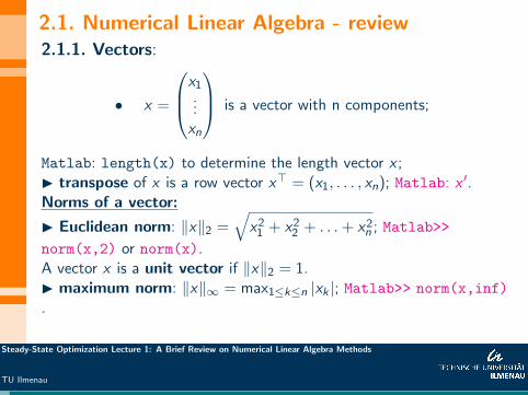
2.1. Numerical Linear Algebra - review2.1.1. Vectors:

• x =

x1...

xn

is a vector with n components;

Matlab: length(x) to determine the length vector x ;I transpose of x is a row vector x> = (x1, . . . , xn); Matlab: x ′.Norms of a vector:

I Euclidean norm: ‖x‖2 =√

x21 + x2

2 + . . .+ x2n ; Matlab>>

norm(x,2) or norm(x).A vector x is a unit vector if ‖x‖2 = 1.I maximum norm: ‖x‖∞ = max1≤k≤n |xk |; Matlab>> norm(x,inf)

.


TU Ilmenau

Operations with vectors

I the result of multiplication of a vector x by a scalar α is vector :αx = (αx1, αx2, . . . , αxn); Matlab>> α ∗ x .For two vectors x any y of equal length:I the sum of x and y: x + y = (x1 + y1, . . . , xn + yn); Matlab>> x+y.I the scalar product of x and y, denoted by < x , y > or x · y or x>y ,is scalar number given by x>y = x1y1 + . . .+ xnyn; Matlab>> x’*y.Note that: x>x = ‖x‖2.I componentwise product of x and y is a vector given by(x1y1, . . . , xnyn); Matlab>> x.*y


TU Ilmenau

Linear Combination, Linear Independencies andBasisI A vector x is a linear combination of vectors v1, v2, . . . , vm in Rn

if there are scalars α1, α2, . . . , αm such that x = α1v1 + . . .+ αmvm.I a set of vectors v1, v2, . . . , vm in Rn are linearly dependent if thereare scalars α1, α2, . . . , αm not all of them equal to zero such that

α1v1 + α2v2 + . . .+ αmvm = 0. (1)

If equation (1) holds true only for α1 = α2 = . . . = αm = 0, thenthese vectors are said to be linearly independent.⇒ The standard unit vectors e>i = (0, . . . , 1, . . . , 0), i = 1, . . . , n,are linearly independent.I a set of vectors linearly independent vectors {v1, v2, . . . , vm} is abasis of Rn if any vector x in Rn can be written as a linearcombination of these vectors. That is, x = α1v1 + . . .+ αnvn.


TU Ilmenau

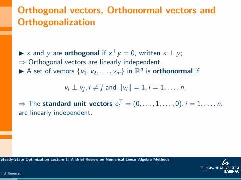
Orthogonal vectors, Orthonormal vectors andOrthogonalization

I x and y are orthogonal if x>y = 0, written x ⊥ y ;⇒ Orthogonal vectors are linearly independent.I A set of vectors {v1, v2, . . . , vm} in Rn is orthonormal if

vi ⊥ vj , i 6= j and ‖vi‖ = 1, i = 1, . . . , n.

⇒ The standard unit vectors e>i = (0, . . . , 1, . . . , 0), i = 1, . . . , n,are linearly independent.


TU Ilmenau

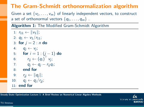
The Gram-Schmidt orthonormalization algorithmGiven a set {v1, . . . , vm} of linearly independent vectors, to constructa set of orthonormal vectors {q1, . . . , qm} .

Algorithm 1: The Modified Gram-Schmidt Algorithm

1: r11 ← ‖v1‖;2: q1 ← v1/r11;3: for j = 2 : n do4: qj ← vj ;5: for i = 1 : (j − 1) do6: rij ← (qi )

> vj ;7: qj ← qj − rijqi ;8: end for9: rjj ← ‖qj‖;

10: qj ← qj/rjj ;11: end for


TU Ilmenau

A Matlab implementation

function Q=ModGrammSchmidt(V)

[n,m]=size(V);

R=zeros(n,m);

Q=zeros(n,m);

r(1,1)=norm(V(:,1));

Q(:,1)= V(:,1)/r(1,1);

for j=2:n

Q(:,j)=V(:,j);

for i=1:(j-1)

R(i,j)=Q(:,i)’*V(:,j);

Q(:,j)=Q(:,j)-R(i,j)*Q(:,i);

end

R(j,j)=norm(Q(:,j));

Q(:,j)=Q(:,j)/R(j,j);

endSteady-State Optimization Lecture 1: A Brief Review on Numerical Linear Algebra Methods

TU Ilmenau

2.1.2. Matrices

A =

a11 a12 . . . a1n

a21 a22 . . . a2n...

.... . . am−1,n

am1 . . . am,n−1 amn

is a matrix with m rows and n columns. A shorter notation A = (aij).I transpose A> is a matrix with n rows and m columns; Matlab>>A’.I rank of A is a number equal to the number of linear independentrows or columns of A; Matlab >> rank(A).Properties:• rank(A) ≤ min{m, n};• if rank(A) = m, then A has full row rank;• if rank(A) = n, then A has full column rank;• If y ∈ Rm and x ∈ Rn, then matrix A = yx> has rank(A) = 1.


TU Ilmenau

Matrix normsLet A ∈ Rm×n; i.e. A is an m by n matrix. ThenI Frobenious norm of A;

‖A‖F =

m∑i=1

n∑j=1

|aij |21/2

; Matlab: norm(A,’fro’).

I Maximum norm of A:

‖A‖∞ = max1 ≤ i ≤ m1 ≤ j ≤ n

|aij |; Matlab: norm(A,inf).

I Induced norm of A:

‖A‖2 = maxx 6=0

‖Ax‖2

‖x‖2= max

x 6=0

‖Ax‖‖x‖

; Matlab: norm(A,2) or norm(A) .

• For any matrix A, the following holds true: ‖A‖2 ≤ ‖A‖F ≤ ‖A‖∞ .


TU Ilmenau

Operations with matricesI sum of two matrices A = (aij) and B = (bij) of equal sizeA + B = (aij + bij); Matlab >> C=A+B.I componentwise product of two matrices A = (aij) and B = (bij)of equal size A. ∗ B = (aij ∗ bij); Matlab >> C=A.*B.I product of a matrix A = (aij) size m× n and matrix B = (bjk) sizen × p is a matrix C = (cik) of size m × p, such that C = AB:

Algorithm 2: Matrix Multiplication

1: for i = 1 : m do2: for k = 1 : p do3: cik =

∑nj=1 aijbjk ;

4: end for5: end for

Matlab>> C=A*B.I product of a matrix A size m × n and vector x of length n is avector b of length m; Matlab>> b=A*x.


TU Ilmenau

Square matrices and some propertiesI an m by n matrix A is a square matrix if m = n;I For the square matrix A, d = (a11, a22, . . . , ann) is the vector ofdiagonal elements; Matlab >> d=diag(A).I the n by n matrix with all it diagonal elements equal to 1 and therest of the elements equal to 0 is the identity matrix In.Note that: ‖In‖2 = ‖In‖F = ‖In‖∞ = 1.Matlab >> I=eye(n).I a n × n matrix A is invertible if there is a matrix B such thatAB = BA = In. B is called the inverse of A; written B = A−1;Matlab>> B=inv(A).I if an n × n matrix A is invertible, then

column vectors A or row vectors of A are linearly independent;Ax = 0 iff x = 0.

rank(A) = n or

det(A) 6= 0; Matlab>> det(A).


TU Ilmenau

Eigenvalues and eigenvectorsA non-zero (real or complex) number λ is an eigenvalue of A if

Av = λv ,

for some vector v . In this case is called an eigenvector of A. Aneigenvalue can be a real or a complex number; Matlab>>[V,D]=eig(A).• One use of eigenvalues: stability analysis of linear and nonlineardynamic systems.

I λ is an eigenvalue of an n×n square matrix A iff det(λI − A) = 0 .

I p(λ) = det(λI − A) = 0 is called characteristic polynomial of A

of degree n.Example:

If A =

[1 23 4

], then p(λ) = det(λI − A) = λ2 − 5λ− 2.


TU Ilmenau

Spectrum and spectral radiusI For a matrix A, the set

σ(A) = {λ | λ is eigenvalue of A}is called the spectrum of the matrix A.I The number of

ρ(A) = maxλ∈σ(A)

|λ|

is called the spectral radius of A.Example:

If A =

[−4 00 3

]Then σ(A) = {−4, 3} and ρ(A) = 4.I For an A ∈ Rn×n, it follows that ‖A‖ =

√ρ(AA>)

I Convergence of iterative algorithms for the solution of a system ofequations Ax = b depend on the spectral radius of the iterationmatrix.


TU Ilmenau

Symmetric, Semi-definite, Orthogonal MatricesI A square matrix A is symmetric if A = A>.⇒ All eigenvalues of a symmetric matrix are real numbers.I An n × n symmetric matrix A is positive semi-definite ifx>Ax ≥ 0, for all x ∈ Rn.⇒ all eigenvalues of a positive semi-definite matrix are non-negativereal numbers.⇒ For any matrix B, the matrix A = BB> is symmetric and positivedefinite.I An n × n symmetric matrix A is positive definite if x>Ax ≥ 0, forall x ∈ Rn, x 6= 0.⇒ All eigenvalues of a positive definite matrix are positive realnumbers.⇒ A positive definite matrix is invertible.I A square matrix Q is orthogonal if QQ> = I .⇒ An orthogonal matrix Q is invertible, Q−1 = Q> and ‖Q‖ = 1 .


TU Ilmenau

Singular Value Decomposition (SVD)I Let A an m × n matrix with rank(A) = r , then A can be expressedas

A = UΣV>

where U an m×m and V is an n× n orthogonal matrices and Σ is anm × n diagonal matrix such that

Σ =

σ1 0 . . . 0σ2 0 . . . 0

. . . 0 . . . 0

σr... . . .

...

0 0 . . . 0 0 . . . 0...

... 0 . . . 00 0 . . . 0 0 . . . 0

,

where σ1 ≥ σ2 ≥ . . . ≥ σrand σ1, σ2, . . . , σr are called

singular values of A ;[U,S,V] = svd(A).


TU Ilmenau

SVD...Image CompressionIn the SVD for A, let U = [u1, u2, . . . , um] ∈ Rm×m andV = [v1, v2, . . . , vn] so that

A = [u1, u2, . . . , um]

σ1 0 . . . 0σ2 0 . . . 0

. . . 0 . . . 0

σr... . . .

...

0 0 . . . 0 0 . . . 0...

... 0 . . . 00 0 . . . 0 0 . . . 0

︸︷︷︸

=Σ

v>1v>2...

v>n

Then A = σ1U1V>1 + σ2U2V>2 + . . .+ σrUrV>r .


TU Ilmenau

SVD...Image Compression ...I The gray-scale values of a digital image are repressed by a matrix A.I The sum A = σ1U1V>1 + σ2U2V>2 + . . .+ σrUrV>r is weighted sumwith decreasing singular values as decreasing weights, sinceσ1 ≥ σ2 ≥ . . . ≥ σr .I Thus dropping some of the terms with smaller weights(singular-values) does not significantly affect image quality but savesstorage space ⇒ image compression.(More on this in the Tutorials!!)

Note that: For a symmetric n × n matrix A it follows that• A = UΣV> implies U = V• The columns of U: U1,U2, . . . ,Un are eigenvectors A.• The singular values σ1, σ2, . . . , σr are eigenvalues of A.• In addition, if A positive semi-definite, then singular values arenon-negative, i.e. σ1 ≥ σ2 ≥ . . . ≥ σr ≥ 0.


TU Ilmenau

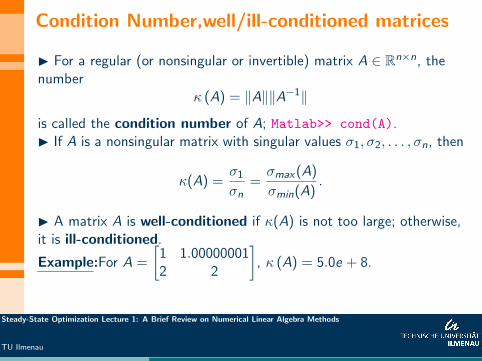
Condition Number,well/ill-conditioned matrices

I For a regular (or nonsingular or invertible) matrix A ∈ Rn×n, thenumber

κ (A) = ‖A‖‖A−1‖

is called the condition number of A; Matlab>> cond(A).I If A is a nonsingular matrix with singular values σ1, σ2, . . . , σn, then

κ(A) =σ1

σn=σmax(A)

σmin(A).

I A matrix A is well-conditioned if κ(A) is not too large; otherwise,it is ill-conditioned.

Example:For A =

[1 1.000000012 2

], κ (A) = 5.0e + 8.


TU Ilmenau

Condition Number,well/ill-conditioned matrices ...Example: Impact of an ill-conditioned matrix.To solve the equation Ax = b with Let

A =

[1000 999999 998

]and b =

[19991997

]Condition number of A : κ(A) = 3.992e + 06.

Solution of Ax = b is x =

[11

].

Now suppose b has a small change (perturbation, noise) given as

b = b + ∆b =

[19991997

]+

[−0.010.01

]The solution of Ax = b will be x =

[20.97−18.99

].

I A small inaccuracy in problem data may lead to a totally differentresult from the actual one.


TU Ilmenau

2.1.3. Solution Methods for Systems of LinearEquationsConsider a system of algebraic equations

Ax = b,

where A is a matrix of size m × n and b is a vector of length.Algorithms to solve Ax = b depend on:

Type of matrix A: eg. square, non-square (i.e. Ax = b is eitherover- or under-determined)

Properties of A: symmetric, nonsymmetric, positive definite,regular (invertible), well-conditioned, ill-conditioned, etc.

Structure of matrix A: dense matrix, sparse-matrix (many zerosthan non-zero numbers), banded matrix, block-structured matrix,etc.

Size of the matrix A: small to medium-sized matrix, very largematrix with a complicated structures, etc.


TU Ilmenau

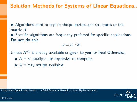
Solution Methods for Systems of Linear Equations...

I Algorithms need to exploit the properties and structures of thematrix A.I Specific algorithms are frequently preferred for specific applications.Do not do this

x = A−1b!

Unless A−1 is already available or given to you for free! Otherwise,

A−1 is usually quite expensive to compute,

A−1 may not be available.


TU Ilmenau

Solution Methods for Systems of Linear Equations...(Simpler Instances)(a) A is a diagonal matrix:

a11 0 . . . 00 a22 0 . . . 0

0 0. . . 0 0

......

. . . 00 0 . . . 0 ann

x1

x2...

xn

=

b1

b2...

bn

,

If all akk 6= 0, then

xk =bk

akk, k = 1, . . . , n.

If for some index k , akk = 0, then the system has no solution.


TU Ilmenau

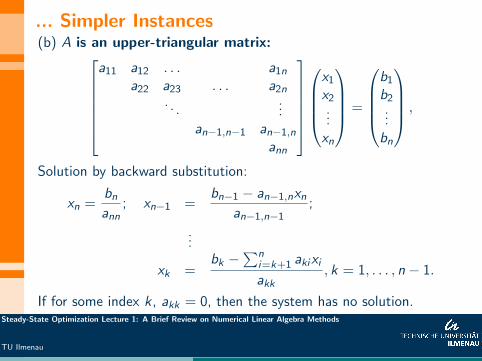
... Simpler Instances(b) A is an upper-triangular matrix:

a11 a12 . . . a1n

a22 a23 . . . a2n

. . ....

an−1,n−1 an−1,n

ann

x1

x2...

xn

=

b1

b2...

bn

,

Solution by backward substitution:

xn =bn

ann; xn−1 =

bn−1 − an−1,nxnan−1,n−1

;

...

xk =bk −

∑ni=k+1 akixi

akk, k = 1, . . . , n − 1.

If for some index k , akk = 0, then the system has no solution.Steady-State Optimization Lecture 1: A Brief Review on Numerical Linear Algebra Methods

TU Ilmenau

...Simpler Instances

I If A a lower-triangular matrix use forward substitution.

(c) A is an orthogonal matrix, then AA> = A>A = In. Thus

Ax = b ⇒ A>Ax = A>b ⇒ Inx = A>b

Hence, the solution of Ax = b is given by

x = A>b.

I In practical applications A may have none of the above simplerstructures.


TU Ilmenau

Solution methods for systems of linear equations...

The choice of an algorithm for the solution of Ax = b depends onwhether:

I A is symmetric or non-symmetricI A positive-definiteI A> is avialbleI A is a square matrixI A is well-conditioned or ill-conditionedI a suitable preconditioner is available for A

In general, there are two classes of algorithms:

I. Direct MethodsII. Iterative Methods

I. Direct Methods

factorize A as a product of matrices with simpler structures(diagonal, triangular, orthogonal matrices, etc.).


TU Ilmenau

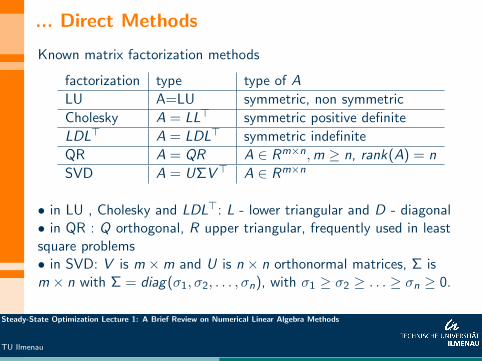
... Direct Methods

Known matrix factorization methods

factorization type type of A

LU A=LU symmetric, non symmetric

Cholesky A = LL> symmetric positive definite

LDL> A = LDL> symmetric indefinite

QR A = QR A ∈ Rm×n,m ≥ n, rank(A) = n

SVD A = UΣV> A ∈ Rm×n

• in LU , Cholesky and LDL>: L - lower triangular and D - diagonal• in QR : Q orthogonal, R upper triangular, frequently used in leastsquare problems• in SVD: V is m ×m and U is n × n orthonormal matrices, Σ ism × n with Σ = diag(σ1, σ2, . . . , σn), with σ1 ≥ σ2 ≥ . . . ≥ σn ≥ 0.


TU Ilmenau

... Direct MethodsExample: Solution through LU factorization

A = LU,

where

L =

∗∗ ∗∗ ∗ ∗...

. . .

∗ ∗ . . . ∗

, U =

∗ ∗ . . . ∗∗ ∗ . . . ∗

. . ....

∗ ∗∗

Then

Ax = b =⇒ (LU)x = b =⇒ L( Ux︸︷︷︸=y

) = b. (2)


TU Ilmenau

... Direct Methods ...

Algorithm 3: Solution of Ax = b through LU factorization

1: Set y = Ux ;2: Use forward substitution to solve for y from Ly = b.;3: Use back substitution to solve for x from Ux = y .

Algorithm 4: Solution of Ax = b through QR factorization

1: Put A = QR so that QRx = b;

2: Multiply both sides of QRx = b by Q> to obtain Rx = Q>b;

3: Use back substitution to solve for x from Rx = d with d = Q>b.


TU Ilmenau

... Direct MethodsAdvantages :

high accuracy of solutions

suitable for small to medium-scale systems of equations

matrix partitioning techniques can be applied

easy to parallelize

Disadvantages :

computationally expensive

inefficient for large and sparse systems

may cause fill-in effect when A is a sparse matrix

Matlab matrix factorization functions :[L,U]=lu(A), L=chol(A), [Q,R]=qr(A), [U,S,V]=svd(A),L = ldl(A) (after MATLAB Version 7.3 (R2006b))


TU Ilmenau

II. Iterative Methods

Algorithm 5: Principle of Iterative Algorithms

1: Step 0: Select an initial iterate x (0);

2: Step k: Determine x (k+1) from x (k), k = 1, 2, . . .;3: Stop: If termination criteria is satisfied.

Commonly used termination criteria: given ε

Relative residual norm:‖b − Ax (k)‖‖b‖

≤ ε.

Two groups of Iterative methods:(A) Stationary Iterative Methods - Matrix Splitting Methods.(B) Dynamic Iterative Methods - Krylov-Subspace Methods.


TU Ilmenau

A. Stationary Iterative Algorithms...

Also known as matrix splitting methods or fixed-point iterativemethods.

Algorithm 6: Basic Algorithm Algorithm

1: Step 0: Start from x0;2: Step k: xk+1 = Bxk + d , k = 1, 2, . . .;3: Stop: If termination criteria is satisfied..

I Well-known algorithms: Jacobi, Gauss-Seidel, SOR, etc.SOR = Successive Over Relaxation.

Jacobi, Gauss-Seidel, SOR MethodsGiven a square matrix A, split A as

A = D + L + U.


TU Ilmenau

Stationary Iterative Algorithms...

L =

0

a21 0a31 a32 0

.... . .

an1 an2 . . . an,n−1 0

,U =

0 a12 . . . a1n

0 a23 . . . a2n

. . ....

0 an−1,n

0

and

D =

a11 0 . . . 00 a22 0 . . . 0

0 0. . . 0 0

......

. . . 00 0 . . . 0 ann

,


TU Ilmenau

Stationary Iterative Algorithms ...

Jacobi method: x (k+1) = Bx (k) + d , whereB = −D−1 (L + U) , d = D−1b.

Gauss-Seidel: x (k+1) = Bx (k) + d , whereB = (D + L)−1 U, d = (D + L)−1 b.

SOR: x (k+1) = Bx (k) + d , withB = (D + ωL)−1 [(1− ω)D − ωU] , d = ω (D + ωL)−1 b,ω > 0 - relaxation factor (convergence tunining factor).

SOR:• Good values for ω are 0 < ω < 2.• 0 < ω < 1 under relaxation.• 1 < ω < 2 over-relaxation.


TU Ilmenau

Stationary Iterative Algorithms ... Convergenceproperties

Convergence from any start point x (0) iff ρ(A) < 1.

A is strictly diagonal dominant =⇒ Jacobi and Gauss-Seidelconverge from any start point x (0).

A symmetric positive definite =⇒ Jacobi and SOR (0 < ω < 2)converge from any start point x (0).

N.B.: Convergence is guaranteed only for a well-conditioned matrix A.

Advantages :

Global convergence if A SPD and ρ(A) < 1.

In general, SOR converges faster than the other two forω ∈ (0, 2).


TU Ilmenau

Stationary Iterative Algorithms - LimitationsDisadvantages :

Applicable only to smaller or problems with well-conditioned orstrictly diagonal dominant matrix A.

Matrix B is not (dynamically) adapted to the current iterate.

May not converge if A is ill-conditioned.

Serious Issues:

What if A is ill-conditioned? I.e. ρ(A) >> 1 or cond(A) >>

What if A is not symmetric?

What if A is not definite?

What if A is not a square matrix?

What if A is very large and sparse matrix?

How to exploit the structure of matrix A? - sparsity, bandstructures, block structures, etc.


TU Ilmenau

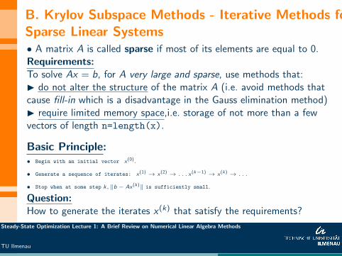
B. Krylov Subspace Methods - Iterative Methods forSparse Linear Systems• A matrix A is called sparse if most of its elements are equal to 0.Requirements:To solve Ax = b, for A very large and sparse, use methods that:I do not alter the structure of the matrix A (i.e. avoid methods thatcause fill-in which is a disadvantage in the Gauss elimination method)I require limited memory space,i.e. storage of not more than a fewvectors of length n=length(x).

Basic Principle:• Begin with an initial vector x(0).

• Generate a sequence of iterates: x(1) → x(2) → . . . x(k−1) → x(k) → . . .

• Stop when at some step k, ‖b − Ax(k)‖ is sufficiently small.

Question:How to generate the iterates x (k) that satisfy the requirements?


TU Ilmenau

B. Iterative Methods for Sparse Linear Systems

Efficient (dynamic) iterative solvers:• Conjugate Gradient method (CG) - for SPD matrix A• Generalized Minimized Residual (GMRES) - for general matrix A• Bi-Conjugate Gradient Stabilized Method (BiCGStab) - fornon-symmetric A (BiCGStab is not discussed here)... ⇒ Krylov Subspace Methods


TU Ilmenau

The Conjugate Gradient method• Initially, invented by Hestens & Steifel in (1959).Standard assumption: A is n × n and SPD, b ∈ Rn.• Let x∗ be a solution of Ax = b. Define the quadratic function

φ(x) =1

2x>Ax − b>x .

Thus, φ can be also written as

φ(x) = φ(x∗) +1

2(x − x∗)> A (x − x∗)︸︷︷︸

≥0

≥ φ(x∗), for any x ∈ Rn.

⇒ φ(x∗) is the minimum value of φ(x). ⇒ The function φ(x) has nodecent at x∗; i.e. ∇φ(x∗) = Ax∗ − b = 0⇒ For an SPD matrix A: Solving the equation Ax = b is equivalentto solving the optimization problem minx ψ(x).


TU Ilmenau

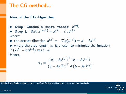
The CG method...

Idea of the CG Algorithm:

• Step: Choose a start vector x (0).• Step k: Set x (k+1) = x (k) − αkd (k)

where:I the decent direction d (k) = −∇φ(x (k)) = b − Ax (k)

I where the step-length αk is chosen to minimize the functionφ(x (k) − αd (k)

)w.r.t. α.

Hence,

αk =

(b − Ax (k)

)> (b − Ax (k)

)(b − Ax (k)

)>A(b − Ax (k)

) .


TU Ilmenau

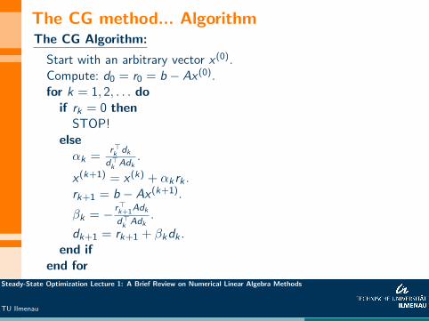
The CG method... AlgorithmThe CG Algorithm:

Start with an arbitrary vector x (0).Compute: d0 = r0 = b − Ax (0).for k = 1, 2, . . . do

if rk = 0 thenSTOP!

elseαk =

r>k dkd>k Adk

.

x (k+1) = x (k) + αk rk .rk+1 = b − Ax (k+1).

βk = − r>k+1Adk

d>k Adk.

dk+1 = rk+1 + βkdk .end if

end forSteady-State Optimization Lecture 1: A Brief Review on Numerical Linear Algebra Methods

TU Ilmenau

The CG method... as a Krylov Subsapce Method• The iterates x(k) of the CG algorithm converge to the unique solution of Ax = bin a maximum of n steps.

• The vectors d0, d1, . . . , dn are conjugate to each other w.r.t. A; i.e. d>i Adj = 0, i 6= j .⇒ The vectors d0, d1, . . . , dn are linearly independent.

F Span{r0, r1, . . . , rk} = Span{r0,Ar0, . . . ,Ak rk

}, k = 0, 1 . . . , n.

F Span{d0, d1, . . . , dk} = Span{r0,Ar0, . . . ,Ak rk

}, k = 0, 1 . . . , n.

I The subspace Kk (r0,A) := Span{r0,Ar0, . . . ,Ak rk

}is called Krylov-subspace (of Rn)

of dimension k + 1.• Recall x(k+1) = x(k) + αk rk = x(0) +

∑kj=0 αj rj

⇒ Using F above

x(k+1) ∈ x(0) +Kk (r0,A), k = 0, 1, . . . , n.

• Thus, CG is a Krylov-subspace method.• Furthermore, the CG method, we have

x(k+1) = x(0) + [r0, r1, . . . , rk ]︸︷︷︸Rk

α0α1

.

.

.αk

= x(0) + Rkηk , where η>k = (α1, α2, . . . , αk )

⇒ The iteration matrix Rk varies.


TU Ilmenau

The Generalized Minimal Residual (GMRES)

Consider again a system of linear equations Ax = b.Assumption: A may not be symmetric.• Given x , the vector r = b − Ax is called the residual vector corresponding to x .• If r = 0, then Ax = b and x a solution of the equation.However, for a large-system of equations Ax = b, finding a solution is not trivial.• Step-by-step minimize the norm of the residual ‖r‖ = ‖b − Ax‖.Basic Algorithm:• Step 0:Start from a vector x(0)

• Step k:Determine x(k) from x(k−1) such that

‖rk‖ = ‖b − Ax(k)‖ ≤ ‖r(k−1)‖ = ‖b − Ax(k−1)‖

• Stop when either ‖rk‖ = 0 or ‖rk‖ is sufficiently small.

Questions: How to construct x (k)’s at each step:• with less computational effort and• every time decreasing the residual vector r?


TU Ilmenau

The Generalized Minimal Residual (GMRES)

Idea of GMRES Method• At each iteration k,(A) determine matrices Vk ,Vk+1 and Hk so that AVk = Vk+1Hk ,

where the columns of Vk = [v1, v2, . . . , vk ] ∈ Rn×k and

Vk+1 = [v1, v2, . . . , vk , vk+1] ∈ Rn×(k+1) are orthonormal vectors and

Hk =

h11 . . . h1k

h21

...

.

.

.

...

.

.

.hkk

hk+1,k

(such a matrix is known as upper Hessenberg matrix of size (k + 1) × k).

(B) Set x(k) = x(0) + Vky(k) , for some y (k).

Question: How to determine the matrices Vk ,Vk+1 and Hk and thevector y (k).


TU Ilmenau

The Generalized Minimal Residual (GMRES)...(a) To determine Vk ,Vk+1 and Hk use the Arnoldi Method.

Algorithm 7: The Arnoldi Algorithm

1: Set r0 = b − Ax(0) 6= 0, and set v1 = r0/‖r0‖.2: for j = 1 to k do3: for i = 1 to j do4: hij = v>i Avj5: end for6: Compute wj = Avj −

∑ji=1 hijvi

7: hj+1,j = ‖wj‖8: if hj+1,j = 0 then9: STOP!10: else11: vj+1 = wj/hj+1,j

12: end if13: end for

• Observe that the Arnoldi algorithm uses steps similar to theGram-Schmidt Orthonormalization process.


TU Ilmenau

The Generalized Minimal Residual (GMRES)...A Matlab code for the Arnoldi Algorithm

function [V,H]=arnoldi(A,r0,k)n=length(A(:,1));V=zeros(n,k+1);H=zeros(k+1,k);V(:,1)=r0/norm(r0);for j=1:k

w=A*V(:,j);for i=1:j

H(i,j)=(V(:,i))’*w;w = w - H(i,j)*V(:,i);

endH(j+1,j)=norm(w);if (H(j+1,j)==0)

break;else

V(:,j+1)=w/H(j+1,j);end

Note that: the matrix V returned from Matlab is Vk+1; while the first k columns of V

belong the matrix Vk .


TU Ilmenau

The Generalized Minimal Residual (GMRES)...Properties of the Arnoldi Algorithm:• The expression AVk = Vk+1Hk is the same as

A [v1, v2, . . . , vk ]︸︷︷︸columns of Vk

= [v1, v2, . . . , vk , vk+1]︸︷︷︸columns of Vk+1

h11 . . . h1k

h21

. . ....

. . .

...hkk

hk+1,k

.

• Observe that

Av1 = h11v1 + h21v2

Av2 = h12v1 + h22v2 + h32v3.

In general, for a vector vj , we have

Avj = h1,jv1 + h2,jv2 + . . .+ hj+1,jvj+1.


TU Ilmenau

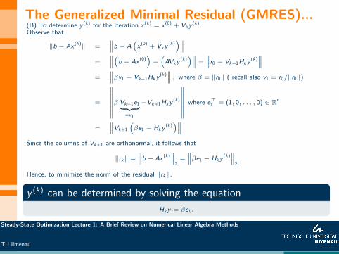
The Generalized Minimal Residual (GMRES)...(B) To determine y (k) for the iteration x (k) = x (0) + Vky

(k).Observe that

‖b − Ax (k)‖ =∥∥∥b − A

(x (0) + Vky

(k))∥∥∥

=∥∥∥(b − Ax (0)

)−(AVky

(k))∥∥∥ =

∥∥∥r0 − Vk+1Hky(k)∥∥∥

=∥∥∥βv1 − Vk+1Hky

(k)∥∥∥ , where β = ‖r0‖ ( recall also v1 = r0/‖r0‖)

=

∥∥∥∥∥∥∥∥β Vk+1e1︸︷︷︸=v1

−Vk+1Hky(k)

∥∥∥∥∥∥∥∥ where e>1 = (1, 0, . . . , 0) ∈ Rn

=∥∥∥Vk+1

(βe1 − Hky

(k))∥∥∥

Since the columns of Vk+1 are orthonormal, it follows that

‖rk‖ =∥∥∥b − Ax (k)

∥∥∥2

=∥∥∥βe1 − Hky

(k)∥∥∥

2

Hence, to minimize the norm of the residual ‖rk‖,

y (k) can be determined by solving the equation

Hky = βe1.


TU Ilmenau

The Generalized Minimal Residual(GMRES)...AlgorithmAlgorithm 8: The GMRES Algorithm

1: Choose initial iterate x(0). Set r0 = b − Ax(0) 6= 0, β = ‖r0‖ and v1 = 1βr0.

2: for j = 1 to k do3: for i = 1 to j do4: hij = v>i Avj5: end for6: w = w − hijvi7: hj+1,j = ‖w‖8: vj+1 = w/hj+1,j .9: end for10: Define the matrix Hk

11: Solve the problem miny ‖βe1 − Hky‖ to obtain y (k)

12: Set x(k) = x(0) + Vky(k).

• The least square problem miny ‖βe1 − Hky‖ is solved by solving Hky = βe1 which is arelatively small Problems.• Use Givens rotation to transform the Hessenberg matrix Hk into an upper triangularmatrix.


TU Ilmenau

GMRES...as a Krylov Subspace MethodObserve in the GMRES Algorithm that:• v1 = r0/‖r0‖; hence, we have Span{v1} = Span{r0} = K0(r0,A).• v2 = 1

h2,1

(Av1 − (v>1 Av1)v1

). This implies

Span{v1, v2} = Span{r0,Ar0} = K1(r0,A).

• In general, inductively, assume that Span{v1, . . . , vj} = Kj (r0,A).We want to show that Span{v1, . . . , vj , vj+1} = Kj+1(r0,A).From the GMRES (or Arnoldi) Algorithm we have

hj+1,jvj+1 = Avj −j∑

i=1

hi,jvi ⇒ hj+1,jvj+1 +

j∑i=1

hi,jvi = Avj

By assumption vj ∈ Kj (r0,A). Consequently Avj ∈ AKj (r0,A) ⊂ Kj+1(r0,A) .

This implies,Span{v1, . . . , vj , vj+1} ⊂ Kj+1(r0,A).

Since both these subspaces have the same dimension, equality holds true.


TU Ilmenau

Some Adivantages/Disadvantages of IterativeMethods

Advantages

usable for large-scale and sparse linear systems

applicable to systems with matrices of arbitrary structures

requires less computer memory

Disadvantages

efficiency depends on the type of problem

difficult to parallelize

require pre-conditioning of the iteration matrices for convergence


TU Ilmenau

Preconditioning - Introduction

• The convergence of iterative methods depends on the condition number of theunderlying matrices.• If the matrix A is ill-conditioned, the solution obtained by an iterative method can be farfrom the true one.• Hence, to improve the performance of an iterative methods it may be necessarypre-condition the matrix A

Preconditioning:Find an matrix P an transform the system Ax = b to

(PA)x = Pb

so that the resulting matrix PA is well-conditioned.Requirement:• the pre-conditioner P should be simple to compute.

• if A is symmetric and positive semi-definite, choose to a convenient P with these

properties


TU Ilmenau

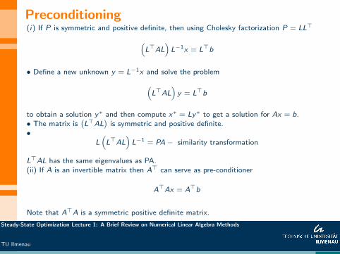
Preconditioning(i) If P is symmetric and positive definite, then using Cholesky factorization P = LL>(

L>AL)L−1x = L>b

• Define a new unknown y = L−1x and solve the problem(L>AL

)y = L>b

to obtain a solution y∗ and then compute x∗ = Ly∗ to get a solution for Ax = b.• The matrix is

(L>AL

)is symmetric and positive definite.

•L(L>AL

)L−1 = PA− similarity transformation

L>AL has the same eigenvalues as PA.(ii) If A is an invertible matrix then A> can serve as pre-conditioner

A>Ax = A>b

Note that A>A is a symmetric positive definite matrix.


TU Ilmenau

Preconditioning...(iii) A diagonal matrix as a scaling pre-conditioner.Define P = diag(p11, p22, . . . , pnn).

If in A = (aij ) such that aii 6= 0, i = 1, . . . , n, then define

pii =1

aii.

The resulting matrix provides a scaling preconditioned for the diagonal elements ofA.

A row scaling pre-conditioner

pii =1∑n

j=1 |aij |, i = 1, . . . , n.

The matrix PA will be a diagonal dominant matrix. (Similarly, a column scalingpre-conditioner).

Additionally, scaling pre-conditioners can be defined using norms of either thecolumn or row vectors of A .

More pre-conditioner types: polynomial pre-conditioners, pre-conditioners based on matrix

splitting, pre-conditioners based on incomplete LU or Cholesky factorization, etc.


TU Ilmenau

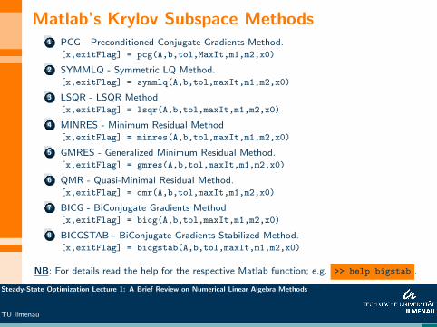
Matlab’s Krylov Subspace Methods1 PCG - Preconditioned Conjugate Gradients Method.

[x,exitFlag] = pcg(A,b,tol,MaxIt,m1,m2,x0)

2 SYMMLQ - Symmetric LQ Method.[x,exitFlag] = symmlq(A,b,tol,maxIt,m1,m2,x0)

3 LSQR - LSQR Method[x,exitFlag] = lsqr(A,b,tol,maxIt,m1,m2,x0)

4 MINRES - Minimum Residual Method[x,exitFlag] = minres(A,b,tol,maxIt,m1,m2,x0)

5 GMRES - Generalized Minimum Residual Method.[x,exitFlag] = gmres(A,b,tol,maxIt,m1,m2,x0)

6 QMR - Quasi-Minimal Residual Method.[x,exitFlag] = qmr(A,b,tol,maxIt,m1,m2,x0)

7 BICG - BiConjugate Gradients Method[x,exitFlag] = bicg(A,b,tol,maxIt,m1,m2,x0)

8 BICGSTAB - BiConjugate Gradients Stabilized Method.[x,exitFlag] = bicgstab(A,b,tol,maxIt,m1,m2,x0)

NB: For details read the help for the respective Matlab function; e.g. >> help bigstab .


TU Ilmenau

References1 J. W. Demmel: Applied numerical linear algebra. SIAM 1997.2 L. N. Trefethen, D. Bau III: Numerical linear algebra. SIAM 1997.3 T. A. Davis Direct methods for sparse linear systems. SIAM 2006.4 Y. Saad: Iterative methods for sparse linear systems. SIAM 2003.5 Y. Saad, M. H. Schultz: GMRES: A generalized minimal residual algorithm for solving nonsymmetric linear

systems. SIAM J. ScI. STAT. COMPUT. Vol. 7, No. 3, July 1986.6 C.T Kelley: Iterative Methods for Linear and Nonlinear Equations. SIAM, 1995.

(http://www.siam.org/books/textbooks/fr16 book.pdf)Matlab codes: http://www.siam.org/books/kelley/fr16/matlabcode.php

7 M. Benzi: Preconditioning Techniques for Large Linear Systems: A Survey. Journal of Computational Physics V.182, pp. 418 – 477, 2002.

8 J. Liesen , Z. Strakos: Krylov subspace methods: principles and analysis. Oxford Univ Press, December 2012.9 V. Simoncini, D. B. Szyld: Recent computational developments in Krylov subspace methods for linear systems

(Review Article). Numer. Linear Algebra Appl. V. 14, pp. 1 – 59 2007.10 Adam Bojanczyk (ed.): Linear algebra for signal processing (Workshop proceedings). Springer, 1995.11 R. V. Patel: Numerical linear algebra techniques for systems and control. IEEE Press, 1994.12 A. Meister: Numerik linearer Gleichungssysteme : eine Einfuhrung in moderne Verfahren. Vieweg, 2008.13 C. Kanzow: Numerik linearer Gleichungssysteme : direkte und iterative Verfahren. Springer, 2005.14 Y. Saad, H. A. van der Vorst: Iterative solution of linear systems in the 20th century. J. of Comput. and Appl.

Math. V. 123, 1–33, 2000.15 R. A. Horn, C. R. Johnson: Topics in matrix analysis. Cambridge Univ. Press, 2007.16 R. A. Horn, C. R. Johnson: Matrix analysis. Cambridge Univ. Press, 2007.17 B. A. Cipra: The Best of the 20th Century - Top 10 Algorithms. SIAM News, Volume 33, Number 4.18 J. R. Schwechuk: An introduction to the conjugate gradient method without an agonizing pain. Technical

Report, Carnegie Mellon University Pittsburgh, PA, USA , 1994.19 H. A. van der Vorst: Bi-CGSTAB: A fast and smoothly converging variant of Bi-CG for the solution of

non-symmetric linear systems. SIAM J. Sci. Stat. Comput., V.13, pp. 631 – 644 , 1992.


TU Ilmenau

Linear Algebra Packages

1 Freely Available Software for Linear Algebra.http://www.netlib.org/utk/people/JackDongarra/la-sw.html

2 Software: Linear Algebra:http://www.scicomp.uni-erlangen.de/archives/SW/linalg.html

3 Lapack++: http://math.nist.gov/lapack++/

4 PARDISO: http://www.pardiso-project.org/

5 MUMPS (aMUltifrontal Massively Parallel sparse directSolver)http://graal.ens-lyon.fr/MUMPS/

6 HSL (Harwell Subroutine Library): http://www.hsl.rl.ac.uk/


TU Ilmenau

steady-state optimization lecture 1: a brief review on ... · steady-state optimization lecture 1:...

Documents