strongly correlated systems in atomic and condensed...

Strongly correlated systems

in atomic and condensed matter physics

Lecture notes for Physics 284

by Eugene Demler

Harvard University

January 25, 2011

Chapter 8

Quantum noisemeasurements as a probe ofmany-body states

8.1 Quantum Noise

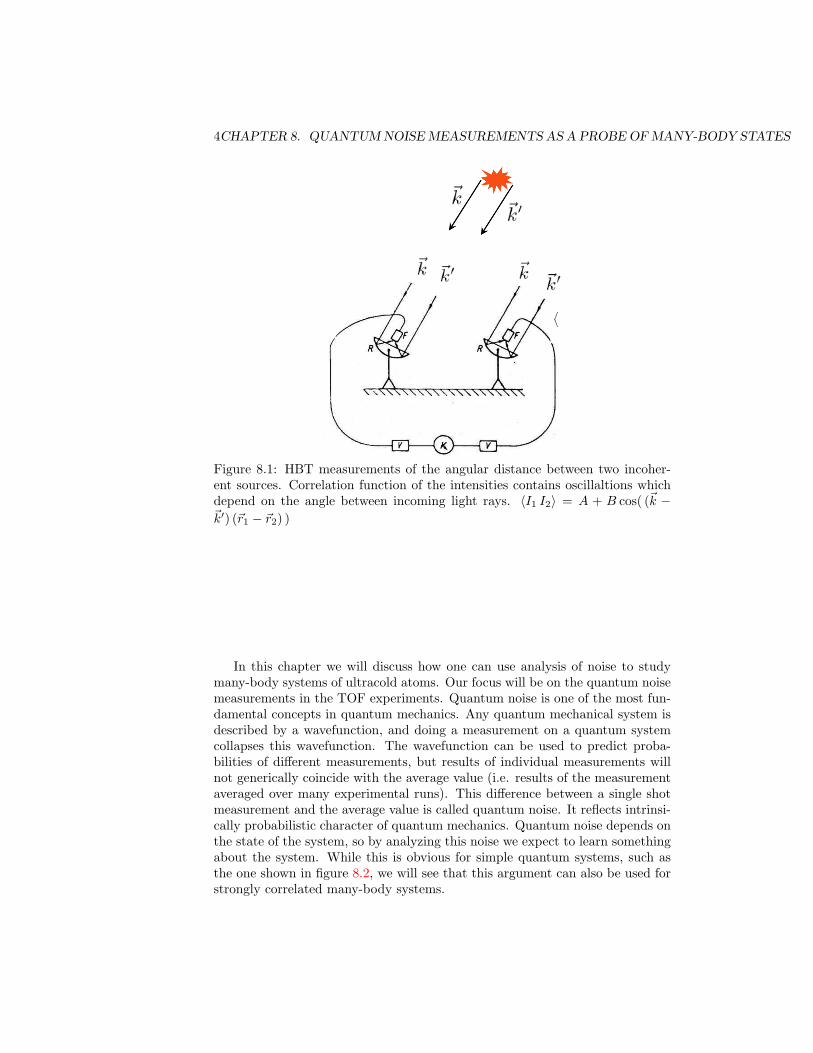
Analysis of noise is a useful tool in many areas of physics. One famous example isHaburry-Brown-Twiss effect used in astronomy. Consider two incoherent distantsources, such as two ends of a star. One can not use a single detector to observeinterference between the sources. When sources are incoherent, a single detectoralways measures the sum of the two intensities. However Haburry-Brown andTwiss realized that one can use two detectors to measure correlations of theintensities[2, 3]. This correlation function now contains an oscillating terms thatdepends on the relative angle of the light rays arriving from the two sources (seefig.8.1). HBT correlations are now commonly used to measure angular diameterof stars[8].

Another canonical example of noise is shot noise in electron transport. Con-sider electric current going through some material, say a simple electrical wire.We can choose a certain cross section of the wire and measure charge goingthrough during time τ . We do such measurements several times and com-pare the results. On the average (i.e. averaged over many runs) this charge is〈Q〉 = 〈I〉τ . But there will also be shot to shot fluctuations. At sufficientlylow temperatures shot noise due to discreetness of electron charge will domi-nate over thermal noise and fluctuations will be given by 〈(Q− 〈Q〉)2〉 = 2eIτ .W. Shottky suggested this as a way of measuring electron charge back in 1918[11]. Currently this technique is used to explore exotic electronic states, suchas fractional quantum Hall states. Noise measurements provided one of thestrongest evidence for the Laughlin picture of the fractional quantum Hall stateby demonstrating that the quasiparticle charge at ν = 1/3 was precisely e/3[9].

3

4CHAPTER 8. QUANTUM NOISE MEASUREMENTS AS A PROBE OF MANY-BODY STATES

Figure 8.1: HBT measurements of the angular distance between two incoher-ent sources. Correlation function of the intensities contains oscillaltions whichdepend on the angle between incoming light rays. 〈I1 I2〉 = A + B cos( (~k −~k′) (~r1 − ~r2) )

In this chapter we will discuss how one can use analysis of noise to studymany-body systems of ultracold atoms. Our focus will be on the quantum noisemeasurements in the TOF experiments. Quantum noise is one of the most fun-damental concepts in quantum mechanics. Any quantum mechanical system isdescribed by a wavefunction, and doing a measurement on a quantum systemcollapses this wavefunction. The wavefunction can be used to predict proba-bilities of different measurements, but results of individual measurements willnot generically coincide with the average value (i.e. results of the measurementaveraged over many experimental runs). This difference between a single shotmeasurement and the average value is called quantum noise. It reflects intrinsi-cally probabilistic character of quantum mechanics. Quantum noise depends onthe state of the system, so by analyzing this noise we expect to learn somethingabout the system. While this is obvious for simple quantum systems, such asthe one shown in figure 8.2, we will see that this argument can also be used forstrongly correlated many-body systems.

8.2. SECOND ORDER CORRELATIONS IN TOF EXPERIMENTS 5

Figure 8.2: Illustration for the idea of quantum noise. A particle is described bya 1d Schroedinger wavefunction. When position of the particle is measured, thiswavefunction is collapsed to a state with a certain position. The wavefunctioncan be used to predict probaiblities to find the particle at different points. Theaverage position is defined as a result of many measurements. Result of anindividual measurement does not generically coincide with what one finds afteraveraging over many shots. The difference between the single shot result andthe average value is called quantum noise.

Figure 8.3: Schematic picture of TOF experiments (courtesy of E. Altman).

8.2 Second order correlations in TOF experi-ments

Our goal is to understand what information can be extracted from the time-of-flight (TOF) experiments. A brief reminder: TOF experiments correspond tosuddenly switching off the confining potential (and the optical lattice potentialif present) and letting an atomic ensemble expand. When the cloud expands toa size which is much larger than its original size, it is imaged by shining a laserbeam (see fig. 8.3). During the expansion the density drops so rapidly that theprobability of atomic collisions quickly becomes negligible. In many cases it isreasonable to assume that during the TOF expansion atoms propagate ballisti-cally. In our discussion in this section we assume that the probability of an atom


to undergo a collision integrated over the entire expansion process is negligible.Then we have a situation when atoms start expanding with velocities that theyhad inside the many-body system and then continue to propagate with preciselythe same velocities. Such assumption is particularly well justified for systemsconfined in optical lattices. In this case atoms have a lot of kinetic energy dueto initial strong confinement within individual wells. Even for systems close toFeshbach resonances (where interactions are strong) ballistic expansion can beachieved by turning off the scattering length right during the expansion usingmagnetic field.

Previously we said that TOF experiments map momentum distribution intoreal space images. Here is a more precise statement: the density of particles atpoint r after the expansion time t is given by the occupation number of particlesin momentum space before the expansion

〈ρσ(r, t)〉 ∝ =(m

~ t

)3

〈nkσ(t = 0)〉 ≡(m

~ t

)3

〈b†kσbkσ〉(t = 0) (8.1)

k(r) =mr

~t(8.2)

These equations assume that expansion of particles is fully ballistic, i.e. thereare no collisions during the expansion time t. We can obtain (8.1), (8.2) byconsidering the time evolution of the operator Ψ†σ(r) in the Heisenberg repre-sentation

Ψ†σ(r, t) =∫

d3k b†kσ(t) eikr =∫

d3k b†kσ(0) ei ( kr−~2k2t2m )

=∫

d3k b†kσ(0) e−i~t2m (~k−m~r~t )2 + imr

22~t (8.3)

When the expansion time is sufficiently long, we can use the steepest descentmethod of integration and find

Ψ†σ(r, t) =(m

~ t

)3/2

b†k(r)σ ei

~2k2(r)t2m (8.4)

From the last equation and the definition of the density operator ρσ(r, t) =Ψ†σ(r, t) Ψσ(r, t) we obtain equations (8.1), (8.2).

In this chapter we will discuss what information can be extracted from TOFimages beyond 〈b†kσbkσ〉. Our focus will be on analyzing second order correlationfunctions

g2σσ′(r, r′) = 〈 δρσ(r) δρσ′(r′) 〉 (8.5)

where

δρσ(r) = ρσ(r, t)− 〈 ρσ(r, t)〉 (8.6)

and 〈. . . 〉 means averaging over many shots. g2 measures correlations in fluctu-ations of the particle number (after TOF expansion). This correlation function

8.2. SECOND ORDER CORRELATIONS IN TOF EXPERIMENTS 7

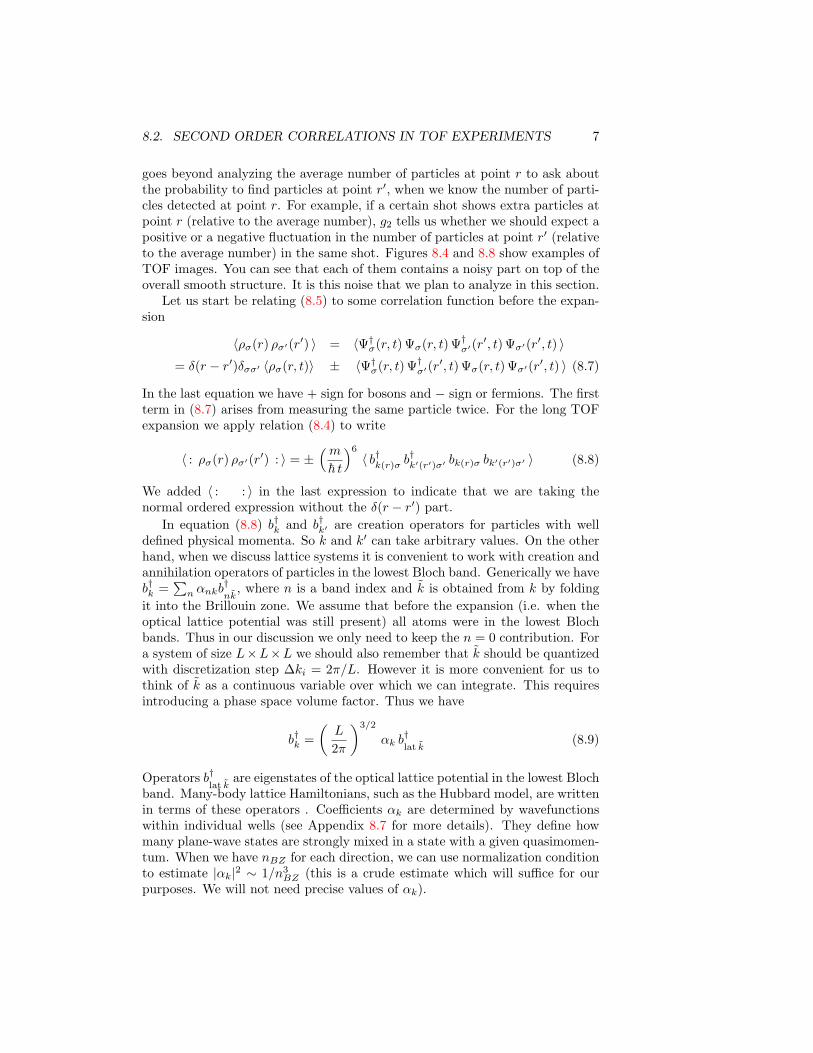
goes beyond analyzing the average number of particles at point r to ask aboutthe probability to find particles at point r′, when we know the number of parti-cles detected at point r. For example, if a certain shot shows extra particles atpoint r (relative to the average number), g2 tells us whether we should expect apositive or a negative fluctuation in the number of particles at point r′ (relativeto the average number) in the same shot. Figures 8.4 and 8.8 show examples ofTOF images. You can see that each of them contains a noisy part on top of theoverall smooth structure. It is this noise that we plan to analyze in this section.

Let us start be relating (8.5) to some correlation function before the expan-sion

〈ρσ(r) ρσ′(r′) 〉 = 〈Ψ†σ(r, t) Ψσ(r, t) Ψ†σ′(r′, t) Ψσ′(r′, t) 〉= δ(r − r′)δσσ′ 〈ρσ(r, t)〉 ± 〈Ψ†σ(r, t) Ψ†σ′(r′, t) Ψσ(r, t) Ψσ′(r′, t) 〉 (8.7)

In the last equation we have + sign for bosons and − sign or fermions. The firstterm in (8.7) arises from measuring the same particle twice. For the long TOFexpansion we apply relation (8.4) to write

〈 : ρσ(r) ρσ′(r′) : 〉 = ±(m

~ t

)6

〈 b†k(r)σ b†k′(r′)σ′ bk(r)σ bk′(r′)σ′ 〉 (8.8)

We added 〈 : : 〉 in the last expression to indicate that we are taking thenormal ordered expression without the δ(r − r′) part.

In equation (8.8) b†k and b†k′ are creation operators for particles with welldefined physical momenta. So k and k′ can take arbitrary values. On the otherhand, when we discuss lattice systems it is convenient to work with creation andannihilation operators of particles in the lowest Bloch band. Generically we haveb†k =

∑n αnkb

†nk̃

, where n is a band index and k̃ is obtained from k by foldingit into the Brillouin zone. We assume that before the expansion (i.e. when theoptical lattice potential was still present) all atoms were in the lowest Blochbands. Thus in our discussion we only need to keep the n = 0 contribution. Fora system of size L×L×L we should also remember that k̃ should be quantizedwith discretization step ∆ki = 2π/L. However it is more convenient for us tothink of k̃ as a continuous variable over which we can integrate. This requiresintroducing a phase space volume factor. Thus we have

b†k =(L

2π

)3/2

αk b†lat k̃

(8.9)

Operators b†lat k̃

are eigenstates of the optical lattice potential in the lowest Blochband. Many-body lattice Hamiltonians, such as the Hubbard model, are writtenin terms of these operators . Coefficients αk are determined by wavefunctionswithin individual wells (see Appendix 8.7 for more details). They define howmany plane-wave states are strongly mixed in a state with a given quasimomen-tum. When we have nBZ for each direction, we can use normalization conditionto estimate |αk|2 ∼ 1/n3

BZ (this is a crude estimate which will suffice for ourpurposes. We will not need precise values of αk).


For example, for the cloud density after the expansion we can write

〈 ρ(r) 〉 =(L

2π

)3 (m~t

)3

|αk|2 〈b†lat k̃ blat k̃ 〉 (8.10)

We define

l =ht

ma(8.11)

A particle with the velocity set by the reciprocal lattice vector, v = h/ma,expands during the time t by l. Then

〈ρ(r)〉 =Nsitesl3|αk|2 〈b†lat k̃ blat k̃ 〉 (8.12)

In a Mott state with n = 1 we have 〈b†lat k̃

blat k̃ 〉 = 1 which gives ρ(r) ≈Nsites/(nBZ l)3. This is an expected result. The cloud size after the expansionis approximately nBZ l in each direction. So we find that the density as thetotal number of atoms divided by the total size of the expanded cloud. This is acrude estimate since the density is not uniform after the expansion. However itshows us that our normalization factors make sense. It will also be useful laterwhen we estimate the magnitude of the noise signal.

We can write for equation (8.8)

〈b†kb†k′bkbk′〉phys = |αk|2 |αk′ |2

(L

2π

)6

〈b†k̃b†k̃′bk̃bk̃′〉lat (8.13)

8.3 Mott state with n = 1

8.3.1 Boson bunching

We have

〈b†k̃b†k̃′bk̃bk̃′〉lat =

1N2

sites

∑lmnρ

〈b†l b†mbnbρ〉 e−ik̃rle−ik̃

′rmeik̃rneik̃′rρ (8.14)

In a Mott state we have local correlations only and

〈b†l b†mbnbρ〉 = δlnδmρ + δlρδmn (8.15)

Then

〈b†k̃b†k̃′bk̃bk̃′〉lat =

1N2

sites

∑lmnρ

( δlnδmρ + δlρδmn ) e−ik̃rle−ik̃′rmeik̃rneik̃

′rρ

=1

N2sites

∑ln

1 +1

N2sites

∑ln

ei(k̃−k̃′)(rn−rl)

(8.16)

8.3. MOTT STATE WITH N = 1 9

We should be careful when doing lattice summation since we have a finite num-ber of sites in the lattice. We have

1N2sites

∑ln

eiq(rn−rl) =1

N2sites

sin2(Nxqxa/2)sin2(qxa/2)

sin2(Nyqya/2)sin2(qya/2)

sin2(Nzqza/2)sin2(qza/2)

(8.17)

We get peaks of height 1 ( use NxNyNz = Nsites) and width ∆qx = 2π/aNx =2π/L. Hence we can write

1N2sites

∑ln

eiq(rn−rl) =(

2πL

)3

δ(q) (8.18)

We can also consider the last equation as taking a continuum limit of the discreetdelta-function for lattice wavevectors.

We have

〈 : ρσ(r) ρσ′(r′) : 〉 =(L

2π

)6 (m~t

)6

|αk|2 |αk′ |2(1 +(

2πL

)3

δ(k − k′ −G))

(8.19)

where k(r) and k′(r′) are given by equation (8.2). Combining this result withequation (8.12) for 〈b†

lat k̃blat k̃ 〉 (we have a Mott state with n = 1) and recalling

that k̃ differs from k by reciprocal lattice vectors G we find

〈 : δρ(r) δρ(r′) : 〉 = (m

~t)6(L

2π

)3

|αk(r)|2 |αk′(r)|2∑G

δ(k(r)− k′(r′)−G)

= (m

~t)6(L

2π

)3

|αk(r)|2 |αk′(r)|2 (a

2π)3∑pn

δ(~r − ~r′

l− ~pn)

=Nsitesl6|αk(r)|2 |αk′(r)|2

∑pn

δ(r − r′

l− pn) (8.20)

Here ~pn = a ~G2π . For a simple cubic lattice we have ~pn of the form

{(1, 0, 0), (0, 1, 0), (0, 0, 1), (1, 1, 0), ..., (2, 0, 0), ...}.We get bunching when k − k′ corresponds to the reciprocal lattice of the

optical lattice. A simple physical interpretation of this result in terms of theHanburry-Brown-Twiss Boson bunching is presented in section 8.3.3. Experi-mental measurements of boson correlations in TOF experiments from the Mottstate are shown in fig. 8.4.

8.3.2 Order of magnitude Estimate

To understand the magnitude of the effect in real experiments we need to dealwith the issue of integrating over the imaging axis. When we take correlation


Figure 8.4: Bosonic bunching in the TOF experiments from the Mott state ofbosons. Figures taken from [5].

functions over two dimensional images we have

g2 2dim(r⊥, r′⊥) =∫

dz dz′ g2(r, r′) (8.21)

Integration over z and z′ picks up contributions which differ in z − z′ = n l.Each of these delta functions contributes l the number of such contributions isnBZ . Hence the total of z and z′ integration is (lnBZ)2. Thus we find

g2 2dim =Nsites

(lnBZ)6(lnBZ)2

∑pn

δ2d(r − r′

l− pn) (8.22)

In experiments it is also more convenient to define

C2 =g2 2dim(r⊥, r′⊥)

〈ρ2dim(r⊥)〉〈ρ2dim(r′⊥)〉(8.23)

Integration over z gives 〈ρ2dim(r⊥)〉 ≈ ρ3dimlnBZ ≈ Nsites/(lnBZ)2. Hence

C2 =1

Nsites

∑pn

δ2d(~r⊥ − ~r′⊥

l− ~pn⊥) (8.24)

To include finite detector resolution we replace

δ2dim(~d

l) =

14π

(l

σ

)2

e−d2/4σ2

(8.25)

8.3. MOTT STATE WITH N = 1 11

Then

C2 =1

4πNsites

(l

σ

)2 ∑pn

e−(~d− tm ~pn)2/4σ2

(8.26)

In typical experiments l/σ ≈ 40 and Nsites ≈ 5 × 105. Thus the signal inC(d) is about 3×10−4. This number agrees with the experimental results shownin fig. 8.4.

8.3.3 Semiclassical picture. Interference of independentcondensates

Our derivation of the boson bunching in (8.20) was based on the fully quantumdescription. In the case of bosons we can also give a classical interpretation ofthis phenomenon.

Let us start with a conceptually simpler problem of interference of two inde-pendent condensates. Such experiments have been among the first experimentsdone with BECs of ultracold atoms[4]. Consider a setup shown in figure 8.5.Two condensates are prepared in traps 1 and 2. At time t = 0 atoms are re-leased, the clouds expand, and the density is measured at point r. We canschematically write for the wavefunction at point r and time t

Ψ(r, t) ∼ eiφ1eim(~r+~d)2

~t + eiφ2eim(~r)2

~t (8.27)

Here φ1 and φ2 are phases of the original condensates before the expansion.Then the density has an interference term

ρint(r) = ei(φ1−φ2)+im~r~d

~t (8.28)

When two condensates are not correlated 〈ei(φ1−φ2)〉 = 0. However this doesnot mean that we do not have interference pattern. It simply means that afteraveraging over many shots interference pattern will disappear. A single shotcan still show a perfect interference pattern (see fig. 8.6). Let us consider twopoint correlation function

〈ρint(r)ρint(r′)〉 = eim~r~d

~t + c.c. (8.29)

We see periodic oscillations in the second order correlation function. This meansthat when we have interference of two uncorrelated condensates, we can notpredict whether point r will have a maximum or a minimum of the interferencepattern. However we can predict that if we find a maximum at point r it willbe followed by another maximum a distance ht/md away. This is an exampleof the ”quantum noise”. Results of an individual measurement are genericallydifferent from averaging over many measurements.

Now imagine a periodic lattice of independent condensates. We can assumethat each condensate has a random phase. When we let all these condensates


Figure 8.5: Schematic picture of interference experiments with two independentcondensates.

to expand we find correlations between all possible pairs. So we can write

〈 δρ(r) δρ(r′) 〉 ∼ 2 cos(m~r

~t~ax) + 2 cos(

m~r

~t2~ax) + 2 cos(

m~r

~t~ay) + · · · (8.30)

We used a{x,y} to denote lattice constants in different directions. When we addup all terms (8.30) we find delta functions at reciprocal lattice vectors as in(8.20).

〈 δρ(r) δρ(r′) 〉 ∼∑G

δ(k(r)− k′(r′)−G) (8.31)

with ~k(r)t/m = r. A ”semiclassical” picture of the Mott state is precisely that:condensates with random uncorrelated phases. Interference experiments witha one dimensional array of uncorrelated condensates have been performed byHadzibabic et al. (see fig. 8.7). The difference of experiments by Hadzibabic etal. [7] with the experiments of Foelling et al. [5] is that the former experimentshave a large number of particles per well and a relatively small number of wells.As a result, individual shots appear to have interference like pattern. One cancheck, however, that this is still noise type correlations by repeating these ex-periments many times. Then one finds that interference patterns averaged overmany shots disappear. By contrast, when the potential between individual wellsis lowered and condensates in different wells begin to establish phase coherencewith each other, interference patterns survive even after averaging over manyshots (see fig. 8.7).

It is also instructive to draw analogy between bosons bunching in TOF exper-iments in optical lattices (see eq. (8.31) ) and the optical HBT effect discussed

8.4. BAND INSULATING STATE OF FERMIONS 13

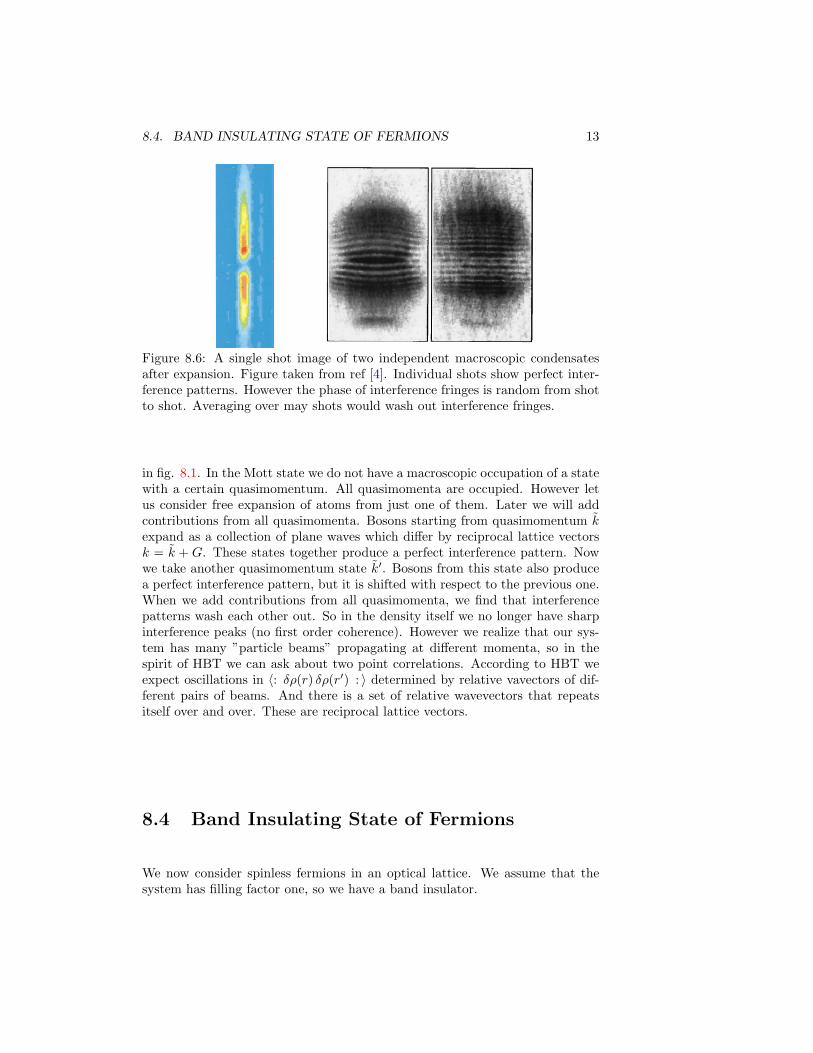
Figure 8.6: A single shot image of two independent macroscopic condensatesafter expansion. Figure taken from ref [4]. Individual shots show perfect inter-ference patterns. However the phase of interference fringes is random from shotto shot. Averaging over may shots would wash out interference fringes.

in fig. 8.1. In the Mott state we do not have a macroscopic occupation of a statewith a certain quasimomentum. All quasimomenta are occupied. However letus consider free expansion of atoms from just one of them. Later we will addcontributions from all quasimomenta. Bosons starting from quasimomentum k̃expand as a collection of plane waves which differ by reciprocal lattice vectorsk = k̃ + G. These states together produce a perfect interference pattern. Nowwe take another quasimomentum state k̃′. Bosons from this state also producea perfect interference pattern, but it is shifted with respect to the previous one.When we add contributions from all quasimomenta, we find that interferencepatterns wash each other out. So in the density itself we no longer have sharpinterference peaks (no first order coherence). However we realize that our sys-tem has many ”particle beams” propagating at different momenta, so in thespirit of HBT we can ask about two point correlations. According to HBT weexpect oscillations in 〈: δρ(r) δρ(r′) : 〉 determined by relative vavectors of dif-ferent pairs of beams. And there is a set of relative wavevectors that repeatsitself over and over. These are reciprocal lattice vectors.

8.4 Band Insulating State of Fermions

We now consider spinless fermions in an optical lattice. We assume that thesystem has filling factor one, so we have a band insulator.


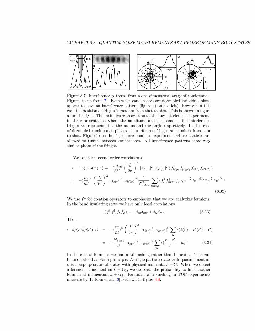
Figure 8.7: Interference patterns from a one dimensional array of condensates.Figures taken from [7]. Even when condensates are decoupled individual shotsappear to have an interference pattern (figure c) on the left). However in thiscase the position of fringes is random from shot to shot. This is shown in figurea) on the right. The main figure shows results of many interference experimentsin the representation where the amplitude and the phase of the interferencefringes are represented as the radius and the angle respectively. In this caseof decoupled condensates phases of interference fringes are random from shotto shot. Figure b) on the right corresponds to experiments where particles areallowed to tunnel between condensates. All interference patterns show verysimilar phase of the fringes.

We consider second order correlations

〈 : ρ(r) ρ(r′) : 〉 = −(m

~t)6(L

2π

)3

|αk(r)|2 |αk′(r)|2 〈 f†k(r) f†k′(r′) fk(r) fk′(r′) 〉

= −(m

~t)6(L

2π

)3

|αk(r)|2 |αk′(r)|21

N2sites

∑lmnρ

〈 f†l f†mfnfρ 〉, e−ik̃rle−ik̃

′rmeik̃rneik̃′rρ

(8.32)

We use f† for creation operators to emphasize that we are analyzing fermions.In the band insulating state we have only local correlations

〈 f†l f†mfnfρ 〉 = −δlnδmρ + δlρδmn (8.33)

Then

〈 : δρ(r) δρ(r′) : 〉 = −(m

~t)6(L

2π

)3

|αk(r)|2 |αk′(r)|2∑G

δ(k(r)− k′(r′)−G)

= −Nsitesl6|αk(r)|2 |αk′(r)|2

∑pn

δ(r − r′

l− pn) (8.34)

In the case of fermions we find antibunching rather than bunching. This canbe understood as Pauli priniciple. A single particle state with quasimomentumk̃ is a superposition of states with physical momenta k̃ + G. When we detecta fermion at momentum k̃ + G1, we decrease the probability to find anotherfermion at momentum k̃ + G2. Fermionic antibunching in TOF experimentsmeasure by T. Rom et al. [6] is shown in figure 8.8.

8.5. TWO PARTICLE INTERFERENCE 15

Figure 8.8: Fermionic antibunching in the TOF experiments from the bandinsulating state of bosons. Figures taken from [6].

8.5 Two particle interference

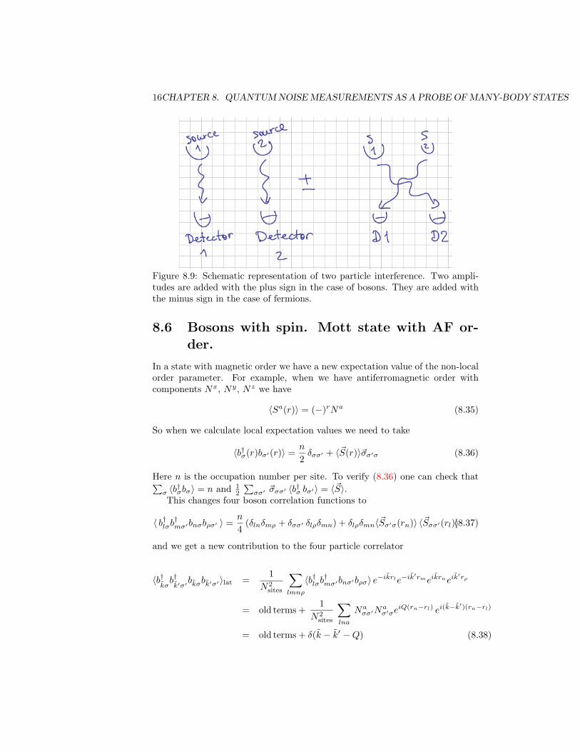
Both bosonic bunching discussed in section 8.3.1 and fermionic antibunching dis-cussed in section 8.4 can be interpreted in terms of the two particle interferenceknown as the Hanburry-Brown-Twiss effect[2, 3, 1]. This is schematically shownin figure 8.9. There are two sources and two detectors. When two particles areobserved in the two detectors, we can have particle in the first detector arrivingfrom the first source, and particle in the second detector arriving from the sec-ond source. Alternatively we can have these particles interchanged. In quantummechanics we need to add the two amplitudes and then take the square to cal-culate the intensity. When the two particles are bosons, we add the amplitudeswith the plus sign. When the particles are fermions, we add the amplitudeswith the minus sign. The cross term of the two amplitudes gives rise to HBTcorrelations [10].


Figure 8.9: Schematic representation of two particle interference. Two ampli-tudes are added with the plus sign in the case of bosons. They are added withthe minus sign in the case of fermions.

8.6 Bosons with spin. Mott state with AF or-der.

In a state with magnetic order we have a new expectation value of the non-localorder parameter. For example, when we have antiferromagnetic order withcomponents Nx, Ny, Nz we have

〈Sa(r)〉 = (−)rNa (8.35)

So when we calculate local expectation values we need to take

〈b†σ(r)bσ′(r)〉 =n

2δσσ′ + 〈~S(r)〉~σσ′σ (8.36)

Here n is the occupation number per site. To verify (8.36) one can check that∑σ 〈b†σbσ〉 = n and 1

2

∑σσ′ ~σσσ′ 〈b†σ bσ′〉 = 〈~S〉.

This changes four boson correlation functions to

〈 b†lσb†mσ′bnσbρσ′ 〉 =

n

4(δlnδmρ + δσσ′ δlρδmn) + δlρδmn〈~Sσ′σ(rn)〉〈~Sσσ′(rl)〉(8.37)

and we get a new contribution to the four particle correlator

〈b†k̃σb†k̃′σ′bk̃σbk̃′σ′〉lat =

1N2

sites

∑lmnρ

〈b†lσb†mσ′bnσ′bρσ〉 e−ik̃rle−ik̃

′rmeik̃rneik̃′rρ

= old terms +1

N2sites

∑lna

Naσσ′Na

σ′σeiQ(rn−rl) ei(k̃−k̃

′)(rn−rl)

= old terms + δ(k̃ − k̃′ −Q) (8.38)

8.7. APPENDIX. HOW TO CALCULATE αNK 17

Figure 8.10: Correlation function in the Mott state of two component Bosemixture with antiferromagnetic order. AF magnetic order manifests itself inthe new peaks at magnetic wavevector.

Here Q is the antiferromagnetic vector (π/a, π/a, π/a). In the noise correlationsof TOF images this should appear as

〈 : δρσ(r) δρσ′(r′) : 〉 = old terms +

(m

~t)6(L

2π

)3

|αk(r)|2 |αk′(r)|2Naσσ′Na

σ′σ

∑G

δ(k(r)− k′(r′)−G−Q)

(8.39)

We see additional peaks at the magnetic wavevector and its Bragg reflections(see fig.8.10. Note that one does not need to do spin resolved measurements tosee magnetic order in this case.

8.7 Appendix. How to calculate αnk

According to the Bloch theorem single particle eigenstates of the periodic po-tential gan be written as (we use 1d case for simplicity)

ψnk(x) = eik̃xunk̃(x) (8.40)

Function unk̃(x) is peridic, i.e. unk̃(x + a) = unk̃(x), where a is the period ofthe potential. Let us now take Fourier transform of (8.40). From periodicity ofunk(x) we have unk(x) =

∑G unkG e

iGx, where G are reciprocal lattice vectors.Thus ∫

dxe−ikxψnk̃(x) =∑G

unk̃Gδ(k − k̃ −G) (8.41)

So a Bloch eigenstate with quasimomentum k̃ involves states with physical mo-mentum k̃ (when G = 0) and other Bragg reflections. The number of Bragg re-flections involved is determined by the Fourier transform of the function unk̃(x).


The latter can be thought of as the wavefunction of a particle inside an individ-ual well. So its Fourier spectrum has a width that is inversely proportional tothe size of the real space wavefunction.

8.8 Problems for Chapter 8

Problem 1In this problem we go back to the collapse and revival experiments with

(spinless) bosonic atoms in an optical lattice (M. Greiner et al. (2002)) discussedin problem 3 in Chapter 6. Previosuly you showed that half-way between revivalsthe system goes through the cat state, in which 〈b〉 = 0 but 〈b2〉 6= 0. Now youneed to propose a method to detect this cat state using noise correlation analysis.

Bibliography

[1] G. Baym. Acta Phys Pol B, 29:1839, 1998.

[2] R.H. Brown and R.Q. Twiss. Nature, 177:27, 1956.

[3] R.H. Brown and R.Q. Twiss. Nature, 178:1447, 1956.

[4] Andrews et al. Science, 275:637, 1997.

[5] S. Foelling et al. Nature, 434:481, 2005.

[6] T. Rom et al. Nature, 444:733, 2006.

[7] Zoran Hadzibabic, Sabine Stock, Baptiste Battelier, Vincent Bretin, andJean Dalibard. Interference of an array of independent bose-einstein con-densates. Phys. Rev. Lett., 93(18):180403, Oct 2004.

[8] HBT. Proc. Roy. Soc. (London) A, 248:222, 19XX.

[9] L. Saminadayar, D. C. Glattli, Y. Jin, and B. Etienne. Observationof the e/3 fractionally charged laughlin quasiparticle. Phys. Rev. Lett.,79(13):2526–2529, Sep 1997.

[10] M. Scully and S. Zubariy. Quantum Optics. Cambridge Univeristy Press,2002.

[11] W. Shottky. Ann. Phys., 57:541, 1918.

19

strongly correlated systems in atomic and condensed...

Documents