structural control of offshore wind turbines
TRANSCRIPT

Emil Smilden
Structural control of offshore windturbinesIncreasing the role of control design in offshorewind farm development
Doctoral thesisfor the degree of philosophiae doctor
Trondheim, May 2019
Norwegian University of Science and TechnologyFaculty of EngineeringDepartment of Marine Technology

Abstract
In recent years, many countries have invested heavily in offshore wind energy. De-spite its widespread adoption, offshore wind energy is still expensive compared toother power generation options, including its onshore counterpart. The wind tur-bines’ support structures, which are comprised of the foundation and wind turbinetower connected by a transition piece, represent a major component of the cost ofoffshore wind energy harnessing. Support structure dimensions are governed byload effects which, in turn, depend on the wind turbine’s control system. In effect,the controls provide a means of reducing the cost of support structures. The overallobjective of this thesis is to develop methods for using the wind turbines’ control sys-tem to make their support structures more economically viable. The focus is on thecurrent and coming generation wind turbines in the double-digit megawatt range,supported by large-diameter monopile foundations.
The methods developed in this thesis can be broadly divided into two categories:(i) control strategies aimed at reducing load effects in support structures, and (ii)design methodology for optimizing the use of these control strategies. The load-reducing controls produce potentially costly side-effects. A major focus of this thesisis to reduce these side-effects at both the turbine and wind farm level. All of the pre-sented work is carried out in the context of a 10MW monopile-supported referencewind turbine located at the Dogger Bank in the North Sea. The majority of the re-sults are obtained from aero-hydro-servo-elastic simulations. Some control theoreticresults are obtained from a reduced-order offshore wind turbine model.
Reducing structural responses by means of collective pitch control—frequentlyreferred to as tower feedback control—is by a wide margin the most effective strat-egy for increasing the fatigue life of support structures. Conventional tower feed-back control has several shortcomings, including undesirable coupling with the windturbine’s basic control system and a limited frequency range of effectiveness. It isfound that these shortcomings can be effectively mitigated by incorporating a pro-portional term (stiffness) into the tower feedback loop. As a result, the side-effectsof tower feedback control are reduced at the turbine level.
Another design methodology that can be useful for reducing the turbine-levelside-effects is event-triggered use of the load-reducing controls. Tradespace explo-ration is employed to examine the effect of different trigger criteria on the trade-offbetween load effect reduction and side-effects. It is found that side-effects can be re-duced by adopting such an approach, depending on the control strategy being usedand the side-effect under consideration. In any case, event-triggered control pro-vides a practical means of achieving a certain level of load effect reduction withoutperforming any turbine-specific tuning of the controls.
In order to reduce side-effects at the wind farm level, it is necessary to customizethe controls for each individual turbine. One option is to customize the controls inconnection with the detailed structural design. In the basic design phase, the sup-port structures are grouped into clusters and designed for the turbine locations giv-
i

ing the highest load effects. In effect, safety margins will differ among the supportstructures within a farm. It is found that the safety margins of support structures canbe effectively equalized by turbine-specific customization of load-reducing controls.Side-effects are then reduced at the wind farm level since they are isolated to thedesign-driving turbine locations.
It is also possible to customize the controls after the turbine is installed. The emer-gence of reliable monitoring systems has enabled the collection of post-installationstructural health data. The present work shows that, for the majority of turbines, apost-installation structural safety assessment will reveal better than expected struc-tural safety performance. Thus, if load-reducing controls have been adopted in thestructural design process, it will be concluded that it is unnecessary to use theseto their fullest potential during actual operation. Consequently, the use of load-reducing controls and their associated side-effects can be significantly reduced atthe wind farm level.
ii

Acknowledgments
This thesis is submitted in partial fulfillment of the requirements for the degree ofphilosophiae doctor (PhD) at the Norwegian University of Science and Technology(NTNU). The work was carried out at the Centre for Autonomous Marine Opera-tions and Systems (NTNU AMOS), which is supported by the Research Council ofNorway through the Centres of Excellence funding scheme, project number 223254.
There are many people without whose support and guidance this work wouldnot have been possible. I would first like to thank Professor Asgeir J. Sørensen forhis support and mentorship over the past several years. His willingness to sharehis expertise, insights, enthusiasm, and life experiences has been essential to mygrowth as a researcher. Furthermore, I would like to thank Associate Professor ErinE. Bachynski for her invaluable help throughout the research and writing of this the-sis. She has always been available to give feedback, answer my questions, or assistin any way possible. I am also grateful to Professor Jørgen Amdahl, whose supportand expertise in offshore structures has been essential to the quality of my research.At NTNU AMOS, I have worked closely with PhD candidate Stian Høegh Sørumand Dr. Jan-Tore Horn. They have contributed tremendously to this thesis both aca-demically and socially.
Professor Jørgen R. Krokstad provided much-appreciated guidance on offshorewind turbine design and hydrodynamics. Discussions with Dr. Lene Eliassen aboutwind turbine aerodynamics helped me lay the foundation for my research. I wouldnot have been able to do the gearbox fatigue calculations without the help of Asso-ciate Professor Amir R. Nejad. Regular meetings with Dr. Bjørn Skaare at Equinorprovided me with invaluable feedback and insight into the offshore wind industryand wind turbine control. I have had numerous interesting conversations about ma-rine control systems with Dr. Astrid H. Brodtkorb. I am also grateful for the manyhours of discussion with PhD candidate Pal Takle Bore about environmental statis-tics and hydrodynamics. The inputs and suggestions of Dr. Karl Merz at SINTEFEnergy were crucial to my understanding of wind turbine dynamics and control.PhD candidate Henrik Schmidt has always been available to share his knowledge ofmathematics and control theory. I have received much-appreciated help with struc-tural dynamics and hydrodynamics from Dr. Ole Nørve Eidsvik and all my ques-tions related to systems engineering have been excellently answered by Dr. SigurdSolheim Pettersen and Dr. Carl F. Rehn.
Finally, I would like to thank my family and friends for the support and encour-agement they have given me. A special thanks goes to my parents Ann-Kristin andBernt, brothers Anders and Einar, and grandparents Inger and Odd.
iii

iv

Contents
1 Introduction 11.1 Motivation and background . . . . . . . . . . . . . . . . . . . . . . . . . 11.2 Research questions and objectives . . . . . . . . . . . . . . . . . . . . . 41.3 Scientific contributions . . . . . . . . . . . . . . . . . . . . . . . . . . . . 41.4 Publications . . . . . . . . . . . . . . . . . . . . . . . . . . . . . . . . . . 51.5 Outline of the thesis . . . . . . . . . . . . . . . . . . . . . . . . . . . . . . 6
2 Offshore Wind Turbine Design Principles 72.1 Environmental descriptions . . . . . . . . . . . . . . . . . . . . . . . . . 8
2.1.1 Wind . . . . . . . . . . . . . . . . . . . . . . . . . . . . . . . . . . 82.1.2 Ocean waves . . . . . . . . . . . . . . . . . . . . . . . . . . . . . 9
2.2 Numerical tools . . . . . . . . . . . . . . . . . . . . . . . . . . . . . . . . 102.2.1 Aerodynamic capabilities . . . . . . . . . . . . . . . . . . . . . . 102.2.2 Hydrodynamic capabilities . . . . . . . . . . . . . . . . . . . . . 112.2.3 Structural capabilities . . . . . . . . . . . . . . . . . . . . . . . . 122.2.4 Control capabilities . . . . . . . . . . . . . . . . . . . . . . . . . . 132.2.5 Validation and verification . . . . . . . . . . . . . . . . . . . . . 13
2.3 Design practices . . . . . . . . . . . . . . . . . . . . . . . . . . . . . . . . 142.3.1 Limit state design . . . . . . . . . . . . . . . . . . . . . . . . . . . 142.3.2 Structural design . . . . . . . . . . . . . . . . . . . . . . . . . . . 162.3.3 Resonance considerations . . . . . . . . . . . . . . . . . . . . . . 16
2.4 Basic offshore wind turbine control . . . . . . . . . . . . . . . . . . . . . 192.4.1 Below-rated operation . . . . . . . . . . . . . . . . . . . . . . . . 192.4.2 Above-rated operation . . . . . . . . . . . . . . . . . . . . . . . . 21
3 Contributions 233.1 Contribution 1 . . . . . . . . . . . . . . . . . . . . . . . . . . . . . . . . . 23
3.1.1 Contribution 1.1 . . . . . . . . . . . . . . . . . . . . . . . . . . . 243.1.2 Contribution 1.2 . . . . . . . . . . . . . . . . . . . . . . . . . . . 26
3.2 Contribution 2 . . . . . . . . . . . . . . . . . . . . . . . . . . . . . . . . . 293.2.1 Contribution 2.1 . . . . . . . . . . . . . . . . . . . . . . . . . . . 29
v

3.2.2 Contribution 2.2 . . . . . . . . . . . . . . . . . . . . . . . . . . . 313.3 Contribution 3 . . . . . . . . . . . . . . . . . . . . . . . . . . . . . . . . . 33
3.3.1 Contribution 3.1 . . . . . . . . . . . . . . . . . . . . . . . . . . . 333.3.2 Contribution 3.2 . . . . . . . . . . . . . . . . . . . . . . . . . . . 34
4 Conclusions and Suggestionsfor Future Work 374.1 Conclusions . . . . . . . . . . . . . . . . . . . . . . . . . . . . . . . . . . 374.2 Suggestions for future work . . . . . . . . . . . . . . . . . . . . . . . . . 39
5 Appended papers 47
vi

List of Figures
2.1 Considerations in the design of offshore wind turbines. . . . . . . . . . 82.2 Outline of a typical aero-hydro-servo-elastic simulation tool. . . . . . . 112.3 Outline of the design process for an offshore wind turbine. . . . . . . . 172.4 Frequencies of interest for selected wind turbines. . . . . . . . . . . . . 182.5 A standard wind turbine power curve . . . . . . . . . . . . . . . . . . . 192.6 Optimal rotor speed for maximum power capture. . . . . . . . . . . . . 20
3.1 Contributions example flowchart. . . . . . . . . . . . . . . . . . . . . . . 233.2 Contribution 1.1 . . . . . . . . . . . . . . . . . . . . . . . . . . . . . . . . 243.3 Overview of control measures for increasing the fatigue life of support
structures. . . . . . . . . . . . . . . . . . . . . . . . . . . . . . . . . . . . 253.4 Contribution 1.2 . . . . . . . . . . . . . . . . . . . . . . . . . . . . . . . . 273.5 Controller robustness parameters as a function of tower feedback gains. 283.6 Tower displacement sensitivities as a function of frequency. . . . . . . . 283.7 Rotor speed sensitivities as a function of frequency. . . . . . . . . . . . 293.8 Modal properties as a function of tower feedback gains. . . . . . . . . . 293.9 Contribution 2.1 . . . . . . . . . . . . . . . . . . . . . . . . . . . . . . . . 303.10 Tradespaces for event-triggered tower feedback control . . . . . . . . . 313.11 Contribution 2.2 . . . . . . . . . . . . . . . . . . . . . . . . . . . . . . . . 323.12 Contribution 3.1 . . . . . . . . . . . . . . . . . . . . . . . . . . . . . . . . 333.13 Circumferential distribution of the support structure’s maximum fa-
tigue utilization for varying site conditions. . . . . . . . . . . . . . . . . 343.14 Contribution 3.2 . . . . . . . . . . . . . . . . . . . . . . . . . . . . . . . . 35
vii

viii

List of Tables
2.1 Basic control objectives in below-rated operation. . . . . . . . . . . . . 202.2 Basic control objectives in above-rated operation. . . . . . . . . . . . . . 21
3.1 Controller performance comparison parameters. . . . . . . . . . . . . . 263.2 Lifetime effects of various control strategies for increasing the fatigue
life of support structures. . . . . . . . . . . . . . . . . . . . . . . . . . . . 263.3 Lifetime effect of peak shaving for increasing the serviceability capac-
ity of support structures. . . . . . . . . . . . . . . . . . . . . . . . . . . . 273.4 Lifetime effects of tower feedback control . . . . . . . . . . . . . . . . . 323.5 Probabilistic outcome of a two-stage adaptation of tower feedback
control. . . . . . . . . . . . . . . . . . . . . . . . . . . . . . . . . . . . . . 353.6 Probabilistic outcome of a two-stage adaptation of peak shaving. . . . 36
ix

x

Chapter 1
Introduction
This chapter introduces and outlines the research problem addressed in this thesis.First, some background and motivation for the research is given. Next, the researchquestions and objectives are presented. Then, the main contributions are summa-rized. Finally, the publications prepared over the course of this thesis work are listedbefore the remaining thesis chapters are outlined.
1.1 Motivation and background
A growing number of countries are investing heavily in wind energy. The majorityof wind farms are located onshore, but over the past decade offshore wind energyhas gained a significant share of the market. While it might appear that offshorewind energy has reached a point where it is considered a fairly safe investment, it isstill in active competition with other power generation options, including its onshorecounterpart. The levelized cost of energy is a measure frequently used to comparedifferent forms of power generation. Even though such estimates are highly uncer-tain, they provide a useful indication of the competitive status of the offshore windindustry. Gas-fired power generation—the benchmark against which renewable en-ergy generation is most often compared—is estimated to cost between $40/MWhand $80/MWh (Milborrow, 2018; Lazard, 2017). Recent estimates place the unsub-sidized generation cost of onshore wind energy between $30/MWh and $60/MWh,thereby suggesting that natural gas is about to be overtaken as the cheapest sourceof energy—at least in some regions of the world (Lazard, 2017; IRENA, 2017; BNEF,2016; Cole et al., 2018). A similar development has taken place in the generation costof solar power which, following a rapid decline over the past years, is now closingin on that of onshore wind. In contrast, the cost of offshore wind energy generationis between $100/MWh and $200/MWh, more than twice that of its onshore coun-terpart (Milborrow, 2018; Cole et al., 2018). The offshore wind industry is expectedto become more cost-competitive over the coming years, but this will require signif-icant efforts from all stakeholders, including the research community.
1

2 CHAPTER 1. INTRODUCTION
While it is difficult to give an exact breakdown of the cost of offshore wind en-ergy generation, some rough estimates can be made. The two major cost componentsare the turbines (∼25%) and operation & maintenance (∼25%), closely followed bysupport structures (∼15%) and assembly & installation (∼15%) (Smith et al., 2015).Wind turbine size is widely considered to be the primary driver of costs. Deployinglarger-sized wind turbines allows for more efficient energy harvesting as the windresource increases with height. But more importantly, it allows the same amount ofpower to be generated with fewer machines, thereby reducing the balance-of-systemcosts (Smith et al., 2015). There is a rapid increase in the size of offshore wind tur-bines. Between 2010 and 2017, the average capacity rating of wind turbines deployedin European waters doubled from 3MW to 6MW (WindEurope, 2010, 2017). It is alsoworth mentioning that 2018 saw the launch of the first commercially available 10MWwind turbine. Not only do these larger turbines require larger equipment and ves-sels for their transportation and installation, but larger foundations are needed tosupport them.1 The adoption of larger turbine sizes therefore goes hand in handwith advances in foundation technologies. Of particular strategic importance is thequestion of which type of foundation to use.
Monopile foundations are widely preferred for their ease of fabrication and in-stallation. More than 80% of wind turbines in European waters are supported bymonopiles (WindEurope, 2017). Jackets are usually the preferred foundation typewhen turbine size or water depth makes monopiles impractical or uneconomical(Seidel, 2014). Improved fabrication processes and installation vessels with increasedpile-driving capacity have extended the application range of monopiles beyond prac-tical limits that were thought to exist only a few years ago (Smith et al., 2015; Seidel,2014). A notable example is the recently commissioned Veja Mate wind farm in theGerman Bight where monopiles support 6MW wind turbines in up to 40m waterdepths. These foundations have a diameter of up to 7.8m (Negro et al., 2017). A num-ber of foundation suppliers are capable of delivering so-called extra-large monopilesand it is expected that monopiles with diameters up to 10m will become a realityin the near future (Smith et al., 2015; Seidel, 2014; Kallehave et al., 2015). Lookingahead, jackets are expected to see their market share increase as wind farms moveinto deeper waters and wind turbines continue to grow in size. The adoption rateof jackets is, however, lower than expected, largely owing to the emergence of extra-large monopiles (Smith et al., 2015).
There are several compelling arguments for extending the application range ofmonopiles rather than adopting other types of foundations (Kallehave et al., 2015;Seidel, 2014). First, developing new supply chains is expensive and time-consuming.The continued use of monopile foundations allows the industry to further developan already mature and well-resourced supply chain. Second, monopiles allow fora high degree of standardization in the supply chain. Thus, there is a large poten-tial for realizing savings through economies of scale and improvements in produc-
1The support structure is broadly comprised of the foundation and wind turbine tower connected bya transition piece.
CHAPTER 1. INTRODUCTION 3
tivity. Third, since many monopiles have been in service for some time, they arebecoming a mature and well-proven technology. The existence of a track record isimportant not only from a technical perspective, but also from an economic per-spective as banks and insurers prefer proven technology. In a long-term perspective,monopiles are generally considered to be an interim solution. The lack of investmentin other foundation technologies could affect the cost of future offshore wind projectsin deeper waters (Catapult, 2015; Smith et al., 2015). The wide range of research anddemonstration projects focused on other technologies, such as floating foundations,are therefore essential to the continued growth of the offshore wind industry beyondthe coming decade. Nevertheless, the focus of this thesis is on methods that can beused to extend the application range of monopiles.
A continued extension of the application range of monopiles presents some chal-lenges. One is simply the size and weight of the foundations. Larger and heavierfoundations are more expensive to fabricate, transport and install. Furthermore,the vessels used for installing the monopiles are typically limited by lifting capac-ity (Seidel, 2014). Reducing the dimensions of monopiles is therefore essential notonly to make them more economically viable, but also to make their installation fea-sible for a wider range of vessels. The wave loads on the foundation poses anotherchallenge. The structural design of large-diameter monopiles is to a large degreegoverned by wave loads. Yet, for economic reasons, the first bending mode of thesupport structure usually occurs at a frequency close to or within the range of waveexcitation frequencies. The wave-induced responses are therefore sensitive to varia-tions in the natural frequencies and damping ratios. Since these parameters dependon the site-specific conditions (soil conditions, water depth), there is a greater needto customize large-diameter monopiles for their specific location in the wind farm.Moreover, their structural design is becoming even more sensitive to uncertaintiesin soil conditions and environmental characteristics (Seidel, 2014).
Support structure dimensions are governed by the ultimate, serviceability, andfatigue loads encountered over the lifetime of the wind turbine. These loads, inturn, depend on the wind turbine’s control system. The fatigue loads depend on theclosed loop properties of the structure (natural frequencies, damping ratios), and theultimate and serviceability loads depend on the operational settings of the turbine(cut-out wind speed, rated wind speed). In effect, the wind turbine’s control systemprovides a means of reducing support structure dimensions. This is most effectivelyachieved by using control strategies aimed specifically at reducing load effects inthe support structure (Bossanyi, 2003; Van der Hooft et al., 2003). While effective,these control strategies have unavoidable side-effects that may reduce or offset po-tential cost savings (Fischer, 2012). Reducing these side-effects is therefore essentialin enabling more widespread use of load-reducing controls.2 Side-effects may be re-duced at both the turbine and wind farm level. Reducing side-effects at the turbinelevel can be achieved by either developing better control strategies or optimizing
2Load-reducing controls is a collective term used to describe control strategies aimed at reducing loadeffects in the support structure.

4 CHAPTER 1. INTRODUCTION
the way control strategies are used. Either way, the overall objective is to achievemaximum load effect reduction with minimum side-effects. Offshore wind turbines,unlike many other mass produced machines, must be designed or at least adaptedspecifically for their intended location. Thus, side-effects can be reduced at the windfarm level by customizing the load-reducing controls for each turbine. Moreover, aturbine-specific customization of the controls can provide a buffer against uncertain-ties and simplifications in the structural design process. Load-reducing controls cantherefore be useful for reducing not only design-driving load effects, but also designconservatism.
1.2 Research questions and objectives
The overall objective of this thesis is to develop methods for using the wind turbines’control system to make their support structures more economically viable. The fo-cus is on large-diameter monopile foundations supporting the current and cominggeneration of wind turbines in the double-digit megawatt range. The methods devel-oped in this thesis all make use of control strategies aimed at reducing load effectsin the support structure. While such control strategies are useful for reducing thecost of support structures, they unavoidably produce side-effects which may reduceor offset potential savings. Hence, a major focus of this thesis is to increase the ef-ficiency of control strategies in terms of their side-effects. The thesis addresses thefollowing research questions:
Q1 How can the wind turbines’ control system be used to reduce the cost of supportstructures?
Q2 How do control strategies for reducing the cost of support structures affect otherwind turbine components and subsystems?
Q3 How can control strategies for reducing the cost of support structures best beused in order to minimize adverse side-effects?
All of the work presented in this thesis is carried out in the context of a 10MWmonopile-supported reference wind turbine located at the Dogger Bank in the NorthSea. The majority of the results are obtained from aero-hydro-servo-elastic simu-lations. Some control theoretic results are obtained from a reduced-order offshorewind turbine model.
1.3 Scientific contributions
In accordance with the overall research objective, the main contribution of this the-sis is methods that make use of the load-reducing capabilities of the wind turbine’scontrol system to make support structures more economically viable. This generalcontribution consists in the development of both new control strategies and meth-ods to increase the efficiency of existing control strategies. The contributions are

CHAPTER 1. INTRODUCTION 5
discussed in greater detail in Chapter 3 and are only briefly summarized here. Thegeneral contributions of this thesis are
C1 Analysis and assessment of the effects of control strategies for reducing the costof support structures.
C2 Methods for increasing the efficiency of load-reducing controls at the wind tur-bine level.3
C3 Methods for increasing the efficiency of load-reducing controls at the wind farmlevel.
1.4 Publications
Several publications have been prepared over the course of this thesis work. Thefollowing journal publications are appended:
P1 Emil Smilden, Erin E. Bachynski, Asgeir J. Sørensen, Jørgen Amdahl (2018). Site-specific Controller Design for Monopile Offshore Wind Turbines Published in theJournal of Marine Structures, 61, 503-523
P2 Emil Smilden, Erin E. Bachynski, Asgeir J. Sørensen, Jørgen Amdahl (2018).Wave Disturbance Rejection for Monopile Offshore Wind Turbines Published inthe Journal of Wind Energy, 22(1), 89-108
P3 Emil Smilden, Stian H. Sørum, Erin E. Bachynski, Asgeir J. Sørensen, JørgenAmdahl (2018). Post-Installation Adaptiation of Offshore Wind Turbine ControlsUnder review for publication in the Journal of Wind Energy
The following publications have been prepared over the course of this thesis work,but are not appended:
Emil Smilden, Erin E. Bachynski, Asgeir J. Sørensen (2017). Key Contributors toLifetime Accumulated Fatigue Damage in an Offshore Wind Turbine SupportStructure. In ASME 2017 36th International Conference on Ocean, Offshore and ArcticEngineering, pages V010T09A075V010T09A075. American Society of MechanicalEngineers.
Emil Smilden, Jan-Tore H. Horn, Asgeir J. Sørensen, Jørgen Amdahl (2016). Re-duced Order Model for Control Applications in Offshore Wind Turbines IFAC-PapersOnLine, 49(23), 386-393.
Emil Smilden, Lene Eliassen, Asgeir J. Sørensen (2016). Wind Model for Simulationof Thrust Variations on a Wind Turbine. Energy Procedia, volume 94, pages 306-318.
3Efficiency refers to the amount of adverse side-effects a control strategy produces in the process ofreducing load effects in the support structure.

6 CHAPTER 1. INTRODUCTION
Emil Smilden, Asgeir J. Sørensen (2016). Application of a Speed Exclusion ZoneAlgorithm on a Large 10MW Offshore Wind Turbine. In ASME 2016 35th Inter-national Conference on Ocean, Offshore and Arctic Engineering, pages V006T09A051-V006T09A051. American Society of Mechanical Engineers.
Stian H. Sørum, Emil Smilden, Jørgen Amdahl, Asgeir J. Sørensen (2018). ActiveLoad Mitigation to Counter the Fatigue Damage Contributions From Unavail-ability in Offshore Wind Turbines. In ASME 2018 37th International Conference onOcean, Offshore and Arctic Engineering, pages V010T09A061-V010T09A061. Amer-ican Society of Mechanical Engineers.
1.5 Outline of the thesis
The thesis is divided into the following chapters:
Chapter 2 - Offshore Wind Turbine Design Principles: The basics of offshore windturbine design are discussed in this chapter. First, the models used to describethe marine environment are presented. Next, numerical tools for offshore windturbine analysis are discussed. Then, key stages and considerations in offshorewind turbine design are discussed. Finally, a description of basic wind turbinecontrol functionality is given.
Chapter 3: Contributions The main contributions of the thesis, which were brieflyintroduced in Chapter 1.3, are discussed in this chapter. Each of these contribu-tions is described in terms of more specific sub-contributions.
Chapter 4: Conclusions and Suggestions for Future Work This chapter concludesthe thesis and provides some suggestions for future work.
Appendix A: Appended Publications

Chapter 2
Offshore Wind Turbine DesignPrinciplesEnvironment, Simulation, and Design Practices
This chapter describes the basics of offshore wind turbine design. First, the modelsused to describe the marine environment are presented. Next, numerical tools foroffshore wind turbine analysis are discussed. Then, the key stages and considera-tions in practical offshore wind turbine design are discussed. Finally, a descriptionof basic wind turbine control functionality is given.
Given the cost-sensitive nature of offshore wind energy harnessing, significanteffort is made to develop cost-effective and reliable designs. Yet, offshore wind tur-bines are subjected to a wide range of stochastic loading conditions over their servicelife. The evaluation of potential designs therefore requires extensive analysis. Nu-merical analysis is widely used for designing offshore wind turbines. In order toidentify critical loading conditions, design guidelines require the consideration ofload cases covering all relevant combinations of environmental conditions (wind,wave, current, ice), operating states (power production, idling, parked, start-up,shut-down, fault occurrences), and accidental states (ship collision, fire) (DNV GLST-0437, 2016). Despite the development of more efficient codes and more powerfulcomputers, numerical analysis remains computationally expensive. Techniques forreducing analysis complexity and the number of simulations are therefore an essen-tial part of offshore wind turbine design.
Figure 2.1 illustrates some of the loading conditions an offshore wind turbine issubjected to over its service life. This thesis is mainly focused on “normal” loadingconditions. Hence, extreme or unusual events and possible deterioration phenom-ena will not receive much attention. Neither will ocean currents or the effects ofinteraction between turbines.
7

8 CHAPTER 2. OFFSHORE WIND TURBINE DESIGN PRINCIPLES
Waves Marine growth
Ice/Ship collision
Scour
Current
Wake effectsTurbulent wind
Wind shear
Controls/Faults
Soil layer 1
Soil layer 2
Soil layer 3
Figure 2.1: Considerations in the design of offshore wind turbines.
2.1 Environmental descriptions
Depending on the application and stage in wind farm development process, envi-ronmental data of varying accuracy may be used. In early-stage activities, such aswind farm prospecting, environmental data may be sourced from publicly availabledatabases, or generated using commercially available software tools. Most stagesof wind farm development, including the structural design process, are, however,carried out using environmental data collected on-site (Burton et al., 2011).
2.1.1 Wind
In general, a fairly accurate representation of the wind’s temporal and spatial vari-ations is needed to properly evaluate the safety and performance of wind turbinesystems. Information about the site-specific wind conditions is often collected usingon-site meteorological towers. In order to capture the wind’s diurnal and seasonalvariability, data from these towers is recorded over at least a one year period. Fur-thermore, inter-annual variability is captured by adjusting the data using long-termrecords from available databases or well-correlated weather stations (Bailey et al.,1997; Brower, 2012). At a given point in space, the wind speed consists of longitu-

CHAPTER 2. OFFSHORE WIND TURBINE DESIGN PRINCIPLES 9
dinal, lateral, and vertical components which may exhibit variations on time scalesranging from seconds to decades (Burton et al., 2011). However, for most practicalpurposes, the wind speed can be described as the sum of its slowly-varying meanvalues and rapidly-varying turbulent components.
The mean longitudinal wind speed, which is directed along the main wind di-rection, is often assumed to be the only non-zero mean component. The wind speeddoes not vary considerably on time scales between those of the short-term variations(turbulence) and diurnal variations. Thus, the mean wind speed can be defined forperiods of ten minutes to a few hours without significant violation of the stationarityassumption (Burton et al., 2011). In this thesis, mean wind speed data with a tempo-ral resolution of three hours is used.
Short-term temporal variations in the wind speed are usually described in termsof statistical properties. Turbulence intensity, defined as the ratio of the wind speed’sstandard deviation to its mean, is a widely used descriptor of the overall level of tur-bulence (Burton et al., 2011). For design purposes, the turbulence intensity is oftentreated as a function of the mean wind speed. In the absence of site-specific data, theturbulence intensity models recommended by design guidelines, such as IEC 61400-1 (2005), may be used. The appropriate choice of turbulence intensity model dependson the site’s wind characteristics. The IEC Class B normal turbulence model, whichis applicable for sites with moderate levels of turbulence, is used in this thesis. Thefrequency content of the turbulence components is described by so-called turbulencespectra. Several models are available for generating time series of three-dimensionalwind fields. The Kaimal and von Karman models make use of a one-dimensionalfast Fourier Transform (FFT) to generate independent time series from turbulencespectra. In contrast, the Mann model makes use of a three-dimensional FFT to gen-erate correlated turbulence components (Burton et al., 2011).
The mean longitudinal wind speed increases with height. This meteorologicalphenomenon — referred to as vertical wind shear—causes load variations at multi-ples of the blade-passing frequency. Wind shear is typically modeled using either alogarithmic or a power law function. The appropriate choice of wind shear modeldepends on the atmospheric conditions and the type of terrain (Burton et al., 2011).The standard IEC 61400-1 (2005) recommends a power law with exponent 0.14 foroffshore conditions.
2.1.2 Ocean waves
Ocean waves consist of a large number of wind-generated components travelling invarious directions. The waves interact with each other, bottom topography, currents,tides, coastlines, islands, and other obstacles, creating a complicated situation. De-scriptions of ocean waves can be very complex depending on the structure underconsideration. Here, the focus is on theories and models that are typically employedin the design of fixed offshore wind turbines.
For most practical applications, ocean waves can be reasonably approximatedwith small-amplitude linear wave theory—often referred to as Airy wave theory.
10 CHAPTER 2. OFFSHORE WIND TURBINE DESIGN PRINCIPLES
The theory is built on the assumption of uniform water depth and potential flow(inviscid, incompressible and irrotational fluid flow) (Faltinsen, 1993). Airy wavetheory is used to simulate irregular sea by considering it as a linear superposition ofindependent long-crested periodic wave trains with different frequencies and direc-tions (Tucker and Pitt, 2001).
The waves’ energy at different frequencies is described by so-called wave spectra.Wave spectra are estimated from short-term wave measurements under the assump-tion that the sea can be described as a stationary random process (Faltinsen, 1993). Anumber of wave spectra are available. The single-peaked Pierson-Morskowitz (PM)and JONSWAP spectra are widely used to describe locally generated waves. Theapplicability of the PM spectrum is limited to fully developed seas, while the JON-SWAP spectrum was developed as a modification of the PM spectrum to account forfetch-limited (developing) seas (DNV GL RP-C205, 2014). Waves are in reality com-posed of both locally and non-locally generated components. A two-peaked spec-trum, such as Torsethaugen’s spectrum, may be applicable in the presence of sig-nificant non-locally generated waves (swell) (DNV GL RP-C205, 2014). The presentwork uses the JONSWAP spectrum which is appropriate for the conditions in theNorth Sea.
Wave conditions can be considered to be stationary for periods of between twentyminutes and six hours. Stationary wave conditions are typically characterized by aset of statistics. The two most frequently used statistics are the significant waveheight and the peak period. The significant wave height is defined as the meanheight of the one-third highest waves, and the peak period is defined as the periodat which the waves have the highest energy density (Faltinsen, 1993).
2.2 Numerical tools
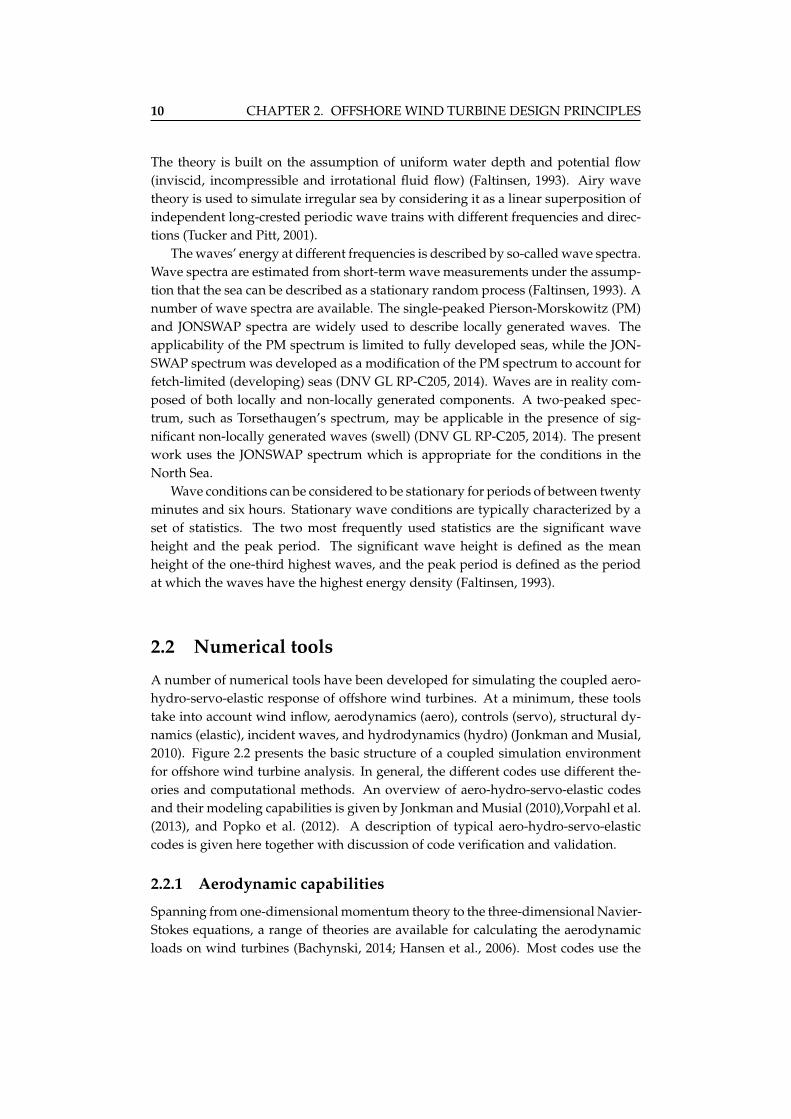
A number of numerical tools have been developed for simulating the coupled aero-hydro-servo-elastic response of offshore wind turbines. At a minimum, these toolstake into account wind inflow, aerodynamics (aero), controls (servo), structural dy-namics (elastic), incident waves, and hydrodynamics (hydro) (Jonkman and Musial,2010). Figure 2.2 presents the basic structure of a coupled simulation environmentfor offshore wind turbine analysis. In general, the different codes use different the-ories and computational methods. An overview of aero-hydro-servo-elastic codesand their modeling capabilities is given by Jonkman and Musial (2010),Vorpahl et al.(2013), and Popko et al. (2012). A description of typical aero-hydro-servo-elasticcodes is given here together with discussion of code verification and validation.
2.2.1 Aerodynamic capabilities
Spanning from one-dimensional momentum theory to the three-dimensional Navier-Stokes equations, a range of theories are available for calculating the aerodynamicloads on wind turbines (Bachynski, 2014; Hansen et al., 2006). Most codes use the

CHAPTER 2. OFFSHORE WIND TURBINE DESIGN PRINCIPLES 11
Wind
Rotor
Drive-train Grid
Controlsystem
Nacelle
Tower
Sub-structure
Foun-dation
Waves
Soil
Rotor-nacelle assembly
Support structure
Figure 2.2: Outline of a typical time-domain numerical analysis tool for simulating the cou-pled aero-hydro-servo-elastic response of offshore wind turbines (A similar figure is presentedby Vorpahl et al. (2013)).
blade element momentum (BEM) method, originally proposed by Glauert (1935).While BEM theory is often chosen for its computational efficiency, it requires sev-eral engineering corrections. Basic corrections are the Prandtl corrections for tip-and hub-loss and the Glauert correction for large induction factors. Furthermore,the codes usually feature semiempirical corrections to account for dynamic stalland dynamic wake effects, and the effects of skewed and sheared inflow conditions(Hansen et al., 2006). A number of codes offer the generalized dynamic wake (GDW)method—described by Peters and He (1991)—as an alternative option to BEM theory.Three-dimensional and unsteady effects such as dynamic wake effects, tip-loss, andskewed wake aerodynamics are inherently accounted for with the GDW method.Since the GDW method was developed under the assumption of a lightly loadedrotor, it suffers from instabilities at low wind speeds. This and other shortcomings,such as the inability to account for wake rotation, have led to the GDW method beingused in combination with BEM theory in practice (Moriarty and Hansen, 2005).
2.2.2 Hydrodynamic capabilities
The hydrodynamic loads on offshore wind turbines include contributions from wavesand current, wave radiation, and higher order effects. Waves can be modeled con-sidering first or higher order incident waves, and with first or higher order wave

12 CHAPTER 2. OFFSHORE WIND TURBINE DESIGN PRINCIPLES
load models (with or without near-field diffraction). How (and whether) these com-ponents are treated depends on the code being used and the type of substructure(Robertson et al., 2014). For fixed offshore wind turbines, the wave kinematics arenormally calculated using Airy linear wave theory, second order Stokes theory, orstream function wave theory. Further, most codes use Morison’s equation to cal-culate the wave loads (Jonkman and Musial, 2010). The hydrodynamic loads onlarge diameter cylinders, such as offshore wind turbine monopile foundations, aredominated by inertia loads. For extra large monopile foundations, diffraction effectsmay come into play (Faltinsen, 1993). A few codes offer the option of calculatingthe first order wave-induced inertia loads using the diffraction theory of MacCamyand Fuchs (1954). While mostly applied for floating offshore wind turbines, an in-creasing number of codes also feature potential flow theory. Potential flow modelsrequire using an offline panel code to compute radiation and diffraction matrices.Since potential flow theory does not account for viscous effects, some codes add thedrag term in Morison’s equation to the solution (Robertson et al., 2017).
2.2.3 Structural capabilities
To capture the fully coupled response, the flexibility of the wind turbine’s rotor, sup-port structure, and preferably drive-train need to be taken into account. Dependingon the code being used, the flexible structural components are modeled using multi-body dynamics formulations, modal representation, finite element formulations, ora combination of these (Vorpahl et al., 2013). Multibody dynamics codes use lumpedmasses connected by multidimensional spring-damper elements to model slenderflexible components like the rotor and support structure. In general, this techniqueis considered less accurate than modal analysis or finite elements models (Buhl et al.,2000). Several popular codes use modal representation to model structural compo-nents. While computationally efficient and reasonably accurate, modal methods donot take into account material and geometrical nonlinearities. In the case of large de-formations, these nonlinearities should not be neglected. An additional drawback ofthese codes is that they require accurate pre-processing of the wind turbine’s modes(Bachynski, 2014). At the expense of computational efficiency, greater accuracy canbe achieved by using finite element models. Most available finite element codes usea nonlinear beam element formulation to model the rotor and support structure. Inaddition to capturing higher modes without pre-processing, this formulation can ac-count for large deformations and geometrical nonlinearities (Bachynski, 2014).
The drive-train dynamics are usually taken into account using multibody dynam-ics formulations. If the shaft’s flexibility is neglected, the drive-train dynamics canbe described using only one rotational degree of freedom. Often, however, it is de-sirable to include a second rotational degree of freedom to capture the first torsionalmode of the drive-train. Typically, the shaft’s flexibility is accounted for by incor-porating a torsional spring-damper element, or an equivalent beam element when afinite element code is used.

CHAPTER 2. OFFSHORE WIND TURBINE DESIGN PRINCIPLES 13
2.2.4 Control capabilities
Wind turbine design standards require the consideration of load cases covering allrelevant design situations, including power production, idling, start-up and shut-down, and fault conditions (DNV GL ST-0437, 2016). At a minimum, wind tur-bine analysis tools should therefore incorporate basic wind turbine control functions,such as blade pitch and generator torque controls, and start-up and shut-down rou-tines. Nearly all state-of-the-art codes incorporate control functions via a dynamiclink library (DLL). In addtion to providing basic control capabilities, these DLLscontain routines that enable the incorporation of external user-defined control func-tions. Depending on which inputs and outputs are included in the DLL, this allowsfor these tools to also be used for control design and analysis. Moreover, additionaldynamics, such as the blade pitch actuation and the generator response, can easilybe embedded as subroutines in the external controller.
2.2.5 Validation and verification
Despite their widespread use, there is still uncertainty surrounding the accuracy ofaero-hydro-servo-elastic codes. Due to a variety of reasons, codes are often verifiedvia code-to-code comparisons (Vorpahl et al., 2013). The first reason is that com-parable full-scale measurements are difficult to obtain in practice. Environmentalconditions are challenging to characterize. Even if data is collected over a longertime period, one may be unable to determine comparable loading conditions. Asecond reason is that it may be difficult to identify the cause of any discrepancies be-tween simulations and measurements. Code-to-code comparisons make it possibleto attribute discrepancies to differences in modeling and code capabilities. A thirdreason is that access to full-scale measurements is limited. The data collected fromin-situ sensors may be incomplete or inaccurate, or the recording period may be ofinsufficient duration to capture all relevant loading conditions. Moreover, for confi-dentiality reasons, wind turbine manufacturers and operators are generally reluctantto share measurement data or to give out any detailed design information.
The OC3, OC4 and OC5 projects constitutes the most comprehensive code veri-fication and validation effort to date (Jonkman and Musial, 2010; Popko et al., 2012;Robertson et al., 2014, 2015, 2017; Popko et al., 2018). A large number of codes havebeen and are being validated and verified through these projects which are carriedout in collaboration between universities, research institutions, and industry. TheOC3 project represented the first major effort aimed at verifying numerical tools foroffshore wind turbine analysis. The focus of this code-to-code comparison projectwas to verify the simulated responses of an offshore wind turbine supported by dif-ferent substructures (monopile, tripod, spar buoy) (Jonkman and Musial, 2010). TheOC4 project was an extension of the OC3 project to cover a wider range of substruc-tures (jacket, semi-submersible) (Popko et al., 2012; Robertson et al., 2014). A detaileddescription of the findings and conclusion of these projects can be found in the re-spective publications. Overall, the comparisons were successful in identifying the

14 CHAPTER 2. OFFSHORE WIND TURBINE DESIGN PRINCIPLES
effect of different approaches in aero-hydro-servo-elastic modeling (Robertson et al.,2017). The ongoing OC5 project has started the work of comparing codes againstexperimental and full-scale measurements. The OC5 project is carried out in threephases, using data from both bottom-fixed and floating systems (Robertson et al.,2017).
2.3 Design practices
The offshore wind industry is relatively new and it is only quite recently that thecertification authorities have issued separate design guidelines for offshore windturbines. Several features differentiate these structures from other fixed offshorestructures. Offshore wind turbine (monopile) foundations have a high horizontal-to-vertical load ratio, meaning that, unlike the foundations of most offshore oil andgas installations, they are moment resisting. Further, they are unique in their highdiameter-to-length ratio, which makes their soil-structure interaction different fromconventional offshore foundations (Bhattacharya, 2014). For these reasons, monopilesare less restrained against pile head rotation and deflection, making them prone tocyclic soil degradation, especially in the upper soil layers. Furthermore, given theirsquat nature, monopiles are prone to failure due to soil collapse under rigid bodyrotations (Lombardi et al., 2013). Offshore wind turbines are also unique in their dy-namic characteristics and loading conditions. The rotor generates a large thrust forceand dynamic loads at the rotor frequency and multiples of the blade-passing fre-quency. Moreover, since the support structure’s lightly damped fundamental bend-ing mode usually falls close to the rotor and wave excitation frequencies, offshorewind turbines exhibit high dynamic sensitivity. Therefore, as opposed to most off-shore structures, fatigue loads are key design-drivers (Bhattacharya, 2014). A finalnoteworthy feature is that offshore wind turbines are considered to be “low-risk”in the sense that they pose little risk to humans or the environment (Vorpahl et al.,2013). Thus, lower factors of safety can be accepted.
2.3.1 Limit state design
An offshore wind turbine may be subjected to a wide range of loading conditionsover its service life. In order to identify critical loading conditions, design guide-lines require the consideration of extensive load cases covering all relevant combina-tions of environmental conditions (wind, wave, current, ice), operating states (powerproduction, idling, parked, start-up, shut-down, fault occurrences), and accidentalstates (ship collision, fire) (DNV GL ST-0437, 2016). Which particular load cases aredesign-driving depends on the type of foundation and the site-specific conditions,such as the water depth and the environmental characteristics. On a broader level,though, some main design-drivers can be identified. Overall, the structural designof support structures is carried out in the context of the following limit states:
Ultimate limit state (ULS): The largest load effects of the support structure cannot

CHAPTER 2. OFFSHORE WIND TURBINE DESIGN PRINCIPLES 15
exceed its load carrying capacities. Ultimate strength analysis involves extensivesimulations, covering plausible extreme loading events, such as extreme environ-mental conditions, fault occurrences, accident occurrences, or a combinations ofthese (DNV GL ST-0437, 2016).
Serviceability limit state (SLS): The deflections and deformations of the supportstructure during normal operation cannot exceed the tolerances for which thewind turbine is designed. Usually, the serviceability criteria are defined in termsof deflections and rotations (tilt) at the pile head and nacelle level, including boththe initial tilt and permanent rotation accumulated over the service life (Carswellet al., 2016; Arany et al., 2015b).
Fatigue limit state (FLS): The fatigue damage accumulated in the support structureover the service life cannot exceed its fatigue resistance capacity. Fatigue strengthanalysis requires the simulation of thousands of load cases to capture the fatiguecontributions from the wide range of “normal” loading conditions encounteredover the service life. For circular foundations, such as monopiles, the compu-tational effort may be reduced by exploiting the structure’s symmetry (Vorpahlet al., 2013).
In general, the fatigue and serviceability requirements lead to excessive load carryingcapacities. Ultimate strength requirements are therefore usually not design-drivingwith exception of the foundation embedment depth, grouted or flanged connections,and possibly some segments near the tower top (Seidel et al., 2016). Still, since theembedded length is a major cost-driver, ultimate strength considerations are impor-tant in reducing the cost of offshore wind energy. The remaining support struc-ture dimensions are often governed by fatigue considerations (Seidel et al., 2016).Whether wind- or wave-induced fatigue loads dominates the fatigue utilization de-pends on the turbine’s size, type of foundation, and water depth. Wind-inducedfatigue loads often dominate in the case of “hydrodynamically transparent” jacketfoundations, or smaller monopile supported turbines (. 5MW) in shallow to mod-erate water depths (. 20m) (Fischer, 2012). Correspondingly, first-order wave loadsare the primary source of fatigue damage for larger turbines (& 5MW) on monopilefoundations in moderate water depths (& 20m), such as the one considered in thisthesis (Smilden et al., 2017). Due to strict maximum tilt requirements, the diameter ofthe foundation may sometimes be governed by serviceability considerations. Theserequirements, set forth by the wind turbine manufacturer, tend to be less strict forfloating wind turbines. It could, therefore, be argued that higher tilt angles shouldbe permitted in order to reduce support structure costs (Arany et al., 2015b; Bhat-tacharya, 2014). Finally, an essential consideration in designing offshore wind tur-bines is the placement of the support structure’s fundamental resonance frequency.This is discussed in further detail in Section 2.3.3.

16 CHAPTER 2. OFFSHORE WIND TURBINE DESIGN PRINCIPLES
2.3.2 Structural design
The process of designing an offshore wind turbine involves interaction between sev-eral stakeholders, including the wind farm owner, wind turbine manufacturer, foun-dation designer, and third-party certification authority (Seidel, 2010). While mostaspects of this complicated process fall outside the scope of this thesis, it has someimportant implications that need to be highlighted. Here, the focus is on structuraldesign and the interaction between the wind turbine manufacturer and the founda-tion designer.
The design process for an offshore wind turbine is outlined in Figure 2.3. Inthe early stages of the conceptual design phase, the information needed for design-ing the wind turbines is collected and detailed in the so-called design basis (Seidel,2010). Based on the information available at the time, a preliminary design is carriedout for the rotor-nacelle assemblies and support structures, which often also includesselecting the type of foundation (Seidel et al., 2016). Current offshore wind projectsuse standard off-the-shelf rotor-nacelle assemblies that offer limited possibilities forproject-specific adaptations. The turbines’ SCADA and control systems are usuallycustomised for the specific project, at least to some extent. Still, few modifications aregenerally made to the rotor-nacelle assemblies throughout the wind farm develop-ment process (Fischer et al., 2012). The support structures’ dimensions are optimisedin an iterative process, involving both the wind turbine manufacturer and founda-tion designer (Seidel et al., 2016). Ideally, the support structures should be optimisedfor their specific location in the wind farm. In practice, however, they are groupedinto clusters and designed for the turbine locations giving the highest load effects(Ziegler et al., 2016). Consequently, the majority of the support structures have ex-cessive margins of safety. Because of the interdependence of aerodynamic and hy-drodynamic load effects, an integrated approach should be adopted for calculatingthe structural loads. Numerical tools like those discussed in Section 2.2 provide themost accurate alternative for fully integrated analysis. Alternatively, for confiden-tiality reasons, a partly integrated approach is sometimes adopted, whereby loads atselected structural interfaces are exchanged between the parties involved (Vorpahlet al., 2013). Detailed design is primarily a continuation of the basic design phase.The design of secondary structures, such as boat landings, access platforms, andJ-tubes, are finalized in this stage. Some location-specific customizations to the sup-port structures may also be made in the detailed design phase (Seidel, 2010; Seidelet al., 2016).
2.3.3 Resonance considerations
Offshore wind turbines are subjected to dynamic loading from a number of sources.In addition to time-varying environmental loads from the sea and air, unbalancedrotating machinery produce significant cyclic loads at the rotor frequency (1P) andblade passing frequency (2P or 3P). The structure’s natural frequencies should ide-ally fall well outside the range of excitation frequencies. However, for economic

CHAPTER 2. OFFSHORE WIND TURBINE DESIGN PRINCIPLES 17
Site-specificconditions
Design basis
PreliminaryRNA design
Tower DesignFoundation
designRNA design
Design checks
OK?
Final design,verification
Conceptual design
Basic design (iterative)
Detailed design and verification
NoNo
Yes
UnspecifiedWT ManufacturerFoundation designer
Figure 2.3: Outline of the design process for an offshore wind turbine (Adapted from IEC61400-3 (2009); Seidel (2010); Seidel et al. (2016)).
reasons, the first bending mode of the support structure often occurs at a frequencyclose to or within the range of rotor and wave excitation frequencies. The degree towhich this bending mode is excited is an important consideration in designing off-shore wind turbines. Typically, one of three design philosophies is adopted for theplacement of the support structure’s fundamental resonance frequency. Nearly allfixed support structures can be classified as “soft-stiff”, meaning that the resonancefrequency lies in between the 1P and 2P/3P frequency ranges. In general, more eco-nomical support structures could be achieved by placing the resonance frequency inthe “soft-soft” range below the rotor and wave excitation frequencies. While manyfloating structures exhibit resonance frequencies in the “soft-soft” range, this is nota feasible option for most fixed structures due to strength requirements. From thepoint of view of structural safety, it is reasonable to place all resonance frequencies inthe “stiff-stiff” range above the rotor excitation frequencies (Arany et al., 2015a). Thebenefits of safer structures rarely offset the additional material costs. Nonetheless,there are examples of monopile foundations which can be described as “stiff-stiff”,for instance at the Sheringham Shoal wind farm off the coast of Norfolk (Hamreet al., 2011; Lombardi et al., 2013).
18 CHAPTER 2. OFFSHORE WIND TURBINE DESIGN PRINCIPLES
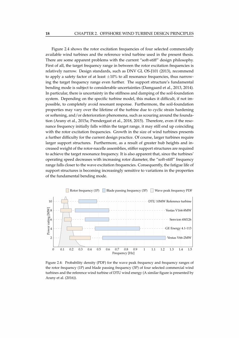
Figure 2.4 shows the rotor excitation frequencies of four selected commerciallyavailable wind turbines and the reference wind turbine used in the present thesis.There are some apparent problems with the current “soft-stiff” design philosophy.First of all, the target frequency range in between the rotor excitation frequencies isrelatively narrow. Design standards, such as DNV GL OS-J101 (2013), recommendto apply a safety factor of at least ±10% to all resonance frequencies, thus narrow-ing the target frequency range even further. The support structure’s fundamentalbending mode is subject to considerable uncertainties (Damgaard et al., 2013, 2014).In particular, there is uncertainty in the stiffness and damping of the soil-foundationsystem. Depending on the specific turbine model, this makes it difficult, if not im-possible, to completely avoid resonant response. Furthermore, the soil-foundationproperties may vary over the lifetime of the turbine due to cyclic strain hardeningor softening, and/or deterioration phenomena, such as scouring around the founda-tion (Arany et al., 2015a; Prendergast et al., 2018, 2015). Therefore, even if the reso-nance frequency initially falls within the target range, it may still end up coincidingwith the rotor excitation frequencies. Growth in the size of wind turbines presentsa further difficulty for the current design practice. Of course, larger turbines requirelarger support structures. Furthermore, as a result of greater hub heights and in-creased weight of the rotor-nacelle assemblies, stiffer support structures are requiredto achieve the target resonance frequency. It is also apparent that, since the turbines’operating speed decreases with increasing rotor diameter, the “soft-stiff” frequencyrange falls closer to the wave excitation frequencies. Consequently, the fatigue life ofsupport structures is becoming increasingly sensitive to variations in the propertiesof the fundamental bending mode.
0 0.1 0.2 0.3 0.4 0.5 0.6 0.7 0.8 0.9 1 1.1 1.2 1.3 1.4 1.5
2
4
6
8
10
Pow
erra
ting
[MW
]
Frequency [Hz]
DTU 10MW Reference turbine
Vestas V164-8MW
Senvion 6M126
GE Energy 4.1-113
Vestas V66-2MW
Rotor frequency (1P) Blade passing frequency (3P) Wave peak frequency PDF
Figure 2.4: Probability density (PDF) for the wave peak frequency and frequency ranges ofthe rotor frequency (1P) and blade passing frequency (3P) of four selected commercial windturbines and the reference wind turbine of DTU wind energy (A similar figure is presented byArany et al. (2016)).

CHAPTER 2. OFFSHORE WIND TURBINE DESIGN PRINCIPLES 19
2.4 Basic offshore wind turbine control
The basics of offshore wind turbine control are presented in the following section.The material is largely based on the handbook of Burton et al. (2011) and the con-trollers developed by NREL and DTU Wind Energy for their reference wind turbines(Bossanyi and Witcher, 2009; Jonkman et al., 2009; Hansen and Henriksen, 2013; Baket al., 2013). These turbines are operated in a conventional variable-speed, variable-pitch configuration. As illustrated in Figure 2.5, the control system of such turbinesbroadly operates in one of two modes depending on the wind speed. These operat-ing modes differ fundamentally in both control objectives and means of actuation. Inbelow-rated wind conditions, the generator torque is varied to maximize power cap-ture via rotor speed control. In above-rated wind conditions, rotor collective pitchcontrol is employed to maintain rated rotor speed, whilst the generator torque iseither kept constant or varied to maintain constant power output. The controllersused in above- and below-rated operation are primarily designed to operate inde-pendently of each other. However, in near-rated wind conditions the control sys-tem is sometimes operated in a combination of the two modes. This is frequentlyreferred to as peak shaving, and the goal is to reduce the maximum aerodynamicthrust which occurs in near-rated wind conditions (Perley et al., 2013).
Windspeed
Power
Cut-outRatedCut-in
Maximum
power
Rated power
operationVariable-speed
operationVariable-pitch
Figure 2.5: A standard wind turbine power curve
2.4.1 Below-rated operation
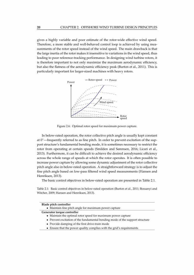
The majority of wind turbines today are equipped with a variable-speed generator,meaning that the generator speed is decoupled from the grid frequency via a powerconverter. This allows for the rotor speed to vary between certain limits. The mainadvantage of variable-speed operation is the possibility to maximize power captureby maintaining the optimal rotor speed (Burton et al., 2011). The most widely usedstrategy for variable-speed operation is to adjust the generator torque as a function ofthe rotor speed to balance the aerodynamic torque at its maximum value. However,as illustrated in Figure 2.6, the optimal rotor speed—for a given rotor—is mainly afunction of the wind speed. Measuring the wind speed at a single point in space
20 CHAPTER 2. OFFSHORE WIND TURBINE DESIGN PRINCIPLES
gives a highly variable and poor estimate of the rotor-wide effective wind speed.Therefore, a more stable and well-behaved control loop is achieved by using mea-surements of the rotor speed instead of the wind speed. The main drawback is thatthe large inertia of the rotor makes it insensitive to variations in the wind speed, thusleading to poor reference-tracking performance. In designing wind turbine rotors, itis therefore important to not only maximize the maximum aerodynamic efficiency,but also the flatness of the aerodynamic efficiency peak (Burton et al., 2011). This isparticularly important for larger-sized machines with heavy rotors.
Power
Rotorspeed
Wind speed
Rotor speed Power
Figure 2.6: Optimal rotor speed for maximum power capture.
In below-rated operation, the rotor collective pitch angle is usually kept constantat 0◦—frequently referred to as fine pitch. In order to prevent excitation of the sup-port structure’s fundamental bending mode, it is sometimes necessary to restrict therotor from operating at certain speeds (Smilden and Sørensen, 2016; Licari et al.,2013). Furthermore, it can be difficult to achieve the desired aerodynamic efficiencyacross the whole range of speeds at which the rotor operates. It is often possible toincrease power capture by allowing some dynamic adjustment of the rotor collectivepitch angle also in below-rated operation. A straightforward strategy is to adjust thefine pitch angle based on low-pass filtered wind speed measurements (Hansen andHenriksen, 2013).
The basic control objectives in below-rated operation are presented in Table 2.1.
Table 2.1: Basic control objectives in below-rated operation (Burton et al., 2011; Bossanyi andWitcher, 2009; Hansen and Henriksen, 2013).
Blade pitch controller• Maintain fine pitch angle for maximum power capture
Generator torque controller• Maintain the optimal rotor speed for maximum power capture• Prevent excitation of the fundamental bending mode of the support structure• Provide damping of the first drive-train mode• Ensure that the power quality complies with the grid’s requirements

CHAPTER 2. OFFSHORE WIND TURBINE DESIGN PRINCIPLES 21
2.4.2 Above-rated operation
Once the generator has reached its rated torque, a different means of actuation is re-quired to control the rotor speed. The control system therefore switches to variable-pitch mode in which the rotor speed is controlled by adjusting the rotor collectivepitch angle. The usual strategy is pitching the blades to feather to reduce the aerody-namic efficiency of the rotor. A conventional proportional-integral (PI) control lawis usually employed to compute the control actions. The controller gains are sched-uled based on the rotor collective pitch angle to take into account the sensitivity ofthe aerodynamic torque to variations in the operating conditions. Furthermore, therotor speed error signal is often low-pass or notch filtered to prevent excitation ofstructural modes and excessive pitch activity at the rotor frequency and multiples ofthe blade-passing frequency (Burton et al., 2011; Hansen and Henriksen, 2013).
In above-rated operation, the generator torque can either be kept constant or var-ied to maintain constant power output. Keeping the generator torque constant isa straightforward strategy with few side-effects or complications. However, due topower quality considerations, it is often desirable to keep the power output constant.This is achieved by simply allowing the generator torque to vary inversely propor-tional to the rotor speed. A potential drawback of constant power operation is thatit induces rotor speed variations. Usually this does not pose a major problem, but itwill to some extent reduce the stability margins of the variable-pitch control loop.
The basic control objectives in above-rated operation are presented in Table 2.2.
Table 2.2: Basic control objectives in above-rated operation (Burton et al., 2011; Bossanyi andWitcher, 2009; Hansen and Henriksen, 2013).
Blade pitch controller• Maintain rated rotor speed• Prevent excitation of the fundamental bending mode of the support structure• Avoid excessive pitch activity
Generator torque controller• Maintain constant power or constant generator torque• Avoid excessive transient drive-train loads• Provide damping of the first drive-train mode• Ensure that the power quality complies with the grid’s requirements

22 CHAPTER 2. OFFSHORE WIND TURBINE DESIGN PRINCIPLES

Chapter 3
Contributions
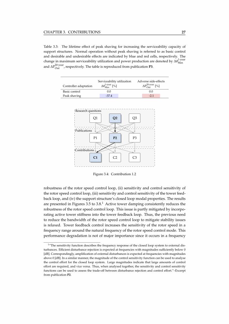
The main contributions of the thesis are discussed in this chapter. The general con-tributions introduced in Chapter 1 are broadly worded. Here, each of these contribu-tions are divided into more specific sub-contributions. Furthermore, in an effort toprovide a better overview, a flowchart like the one in Figure 3.1 is presented for eachsub-contribution. The flowchart highlights what reasearch question(s) motivated thecontribution and in what publication(s) the contribution can be found. The exampleflowchart is for a sub-contribution of C1 which was motivated by research questionQ2 and can be found in publication P2.
Q1 Q2 Q3
P1 P2 P3
C1 C2 C3
Research questions
Publications
Contributions
Figure 3.1: Contributions example flowchart.
3.1 Contribution 1
C1: Analysis and assessment of the effects of control strategies for reducing the cost of sup-port structures.
23

24 CHAPTER 3. CONTRIBUTIONS
The first main contribution of this thesis is concerned with (Q1) how to utilizethe wind turbines’ control system to reduce the cost of their support structures, and(Q2) how doing so affects other wind turbine components and subsystems. Theseunderlying questions are addressed in all three publications P1, P2, and P3.
3.1.1 Contribution 1.1
Analysis and assessment of the lifetime effects of control strategies capable of reducing thecost of support structures.
Q1 Q2 Q3
P1 P2 P3
C1 C2 C3
Research questions
Publications
Contributions
Figure 3.2: Contribution 1.1
Publication P1 presents an overview of different control measures for increasingthe fatigue life of support structures, classified according to their operating regimesand their applicability with respect to different sources of fatigue loads. A summaryis presented in Figure 3.3. Based on a literature review, the control strategies bestsuited for reducing fatigue loads in the reference support structure are identified.These are: (i) tower feedback control (TFC) for reducing fatigue loads in the fore-aft direction during power production, (ii) active generator torque control (AGT) forreducing fatigue loads in the side-side direction during power production, (iii) ac-tive idling (AIC) for reducing fatigue loads in the fore-aft direction during idling,and (iv) soft cut-out (SCO) for reducing fatigue loads in the fore-aft direction duringoperation in above-cut-out wind speeds. A simulation procedure and a set of con-troller performance comparison parameters is developed to assess the lifetime effectsof these control strategies on various wind turbine components and subsystems, in-cluding the support structure. The controller performance comparison parametersare summarized in Table 3.1 and the lifetime effects of the various control strategiesare presented in Table 3.2. The fatigue life of the support structure is approximatelydoubled when all four control strategies are employed. Tower feedback control andactive idling yield the largest increases in the support structure’s fatigue life with

CHAPTER 3. CONTRIBUTIONS 25
contributions of approximately 55% and 35%, respectively. Regardless of the controlstrategy used, there are adverse side-effects, some of which are significant. Towerfeedback control has several adverse side-effects, including increased use of the pitchactuators, increased fatigue loads in the pitch systems, and increased fatigue loadsin drive-train module including the gearbox assembly. Furthermore, active genera-tor torque control causes increased fatigue loads in the drive-train module, and in-creased variability in the power output. Active idling and soft cut-out do not causeany significant adverse side-effects. Notably, the power output is not significantlyaffected by any of the control strategies. The lifetime effects of tower feedback con-trol are also analysed in publications P2 and P3. The results are largely in line withthose of publication P1.
The lifetime effects of peak shaving to increase the support structures’ service-ability capacity are analysed in publication P3. As seen from Table 3.3, it is possibleto increase the serviceability capacity of support structures by approximately 40%with peak shaving. Since peak shaving is achieved by reducing the rotor’s aero-dynamic efficiency, its main adverse side-effect is reduced energy yield. Althoughthese power losses only occur for a relatively small range of wind speeds, they occurin conditions that contribute significantly to the lifetime energy yield. Peak shavingtherefore has a considerable effect in terms of lost power production. Without fur-ther actions being taken, it is unlikely that the cost savings enabled by increasing theserviceability capacity could offset the loss of power production revenue.
Below-rated operation Above-rated operation
Cut-outRatedCut-in
Active Generator Torque (AGT)
Individual pitch control
Soft cut-out (SCO)
Active idling (AIC)
Tower feedback control (TFC)
Passive structural damping device
Semi-active structural damping device
Side-side
Fore-aft
Fore-aft/
Side-sideWindspeed
WTG available WTG unavailable
Figure 3.3: Control measures for increasing the fatigue life of support structures, classifiedaccording to their operating regimes and primary direction of effectiveness. Black arrowsindicate control measures that require the wind turbine generator (WTG) to be available andgrey arrows indicate control measures that are effective independent of the operational stateof the turbine. The figure is reproduced from publication P1.

26 CHAPTER 3. CONTRIBUTIONS
Table 3.1: Controller performance comparison parameters and their desired trend, classifiedaccording to system component. A downward pointing arrow indicates that it is desirable toreduce the performance parameter, and vice versa. The table is reproduced from publicationP1.
Component Performance parameter Description Desired trend
Supportstructure
D20Max Maximum fatigue damage ↓
D20FA Fore-aft fatigue damage ↓
D20SS Side-side fatigue damage ↓
Blade rootDEL20
Edge Edgewise fatigue loads ↓DEL20
Flap Flapwise fatigue loads ↓
Pitch actuatorsDEL20
β Actuator bearing fatigue loads ↓ADC20
β Actuator duty cycle ↓
Drive-trainDEL20
Gear Gear tooth fatigue loads ↓DEL20
Shaft Shaft fatigue loads ↓
Power outputP20
Out Power output ↑P20
Std Standard deviation of power output ↓
Table 3.2: . The lifetime effects of various control strategies for increasing the fatigue life ofsupport structures. The controller performance comparison parameters are given in percent-age [%] of operation with the basic wind turbine controller (BC) and desirable and undesirableeffects are indicated by blue and red cells, respectively. An explanation of the different perfor-mance parameters is given in Table 3.1. The table is reproduced from publication P1.
Support structure Blade root Pitch actuators Drive-train Power outputD20
Max D20FA D20
SS DEL20Edge DEL20
Flap DEL20β ADC20
β DEL20Gear DEL20
Shaft P20Out P20
Std
BC 0.0 0.0 0.0 0.0 0.0 0.0 0.0 0.0 0.0 0.0 0.0TFC -27.8 -27.6 -8.9 -5.0 -4.6 +30.8 +192.8 +0.3 +9.2 0.0 +0.2AGT -9.1 -0.4 -60.1 -22.1 -1.2 -0.7 -2.8 +0.1 +2.4 0.0 +4.0SCO -2.9 -3.0 +0.1 0.0 -0.3 0.0 +0.2 0.0 +0.8 +0.1 0.0AIC -17.9 -23.5 +2.8 +0.1 -1.4 0.0 0.0 0.0 +1.1 0.0 0.0All -52.4 -51.3 -60.7 -21.4 -6.7 +30.8 +194.0 +0.4 +12.4 +0.1 +3.8
3.1.2 Contribution 1.2
Analysis and assessment of the interactions between basic operation and tower feedback con-trol.
Controlling the support structure’s loads will, to some extent, interfere with thebasic operation of the wind turbine. In particular, interaction between control loopswith conflicting control objectives can degrade performance and cause stability is-sues. The interaction between tower feedback control and the wind turbine’s basiccontrol system is analysed in publication P2. Using a reduced-order offshore windturbine model, some fundamental closed loop properties are analysed. These are: (i)
CHAPTER 3. CONTRIBUTIONS 27
Table 3.3: The lifetime effect of peak shaving for increasing the serviceability capacity ofsupport structures. Normal operation without peak shaving is referred to as basic controland desirable and undesirable effects are indicated by blue and red cells, respectively. Thechange in maximum serviceability utilization and power production are denoted by ∆θ
1-yearMax
and ∆P20-yearOut , respectively. The table is reproduced from publication P3.
Serviceability utilization Adverse side-effects
Controller adaptation ∆θ1-yearMax [%] ∆P20-year
Out [%]
Basic control 0.0 0.0Peak shaving -37.4 -2.1
Q1 Q2 Q3
P1 P2 P3
C1 C2 C3
Research questions
Publications
Contributions
Figure 3.4: Contribution 1.2
robustness of the rotor speed control loop, (ii) sensitivity and control sensitivity ofthe rotor speed control loop, (iii) sensitivity and control sensitivity of the tower feed-back loop, and (iv) the support structure’s closed loop modal properties. The resultsare presented in Figures 3.5 to 3.8.1 Active tower damping consistently reduces therobustness of the rotor speed control loop. This issue is partly mitigated by incorpo-rating active tower stiffness into the tower feedback loop. Thus, the previous needto reduce the bandwidth of the rotor speed control loop to mitigate stability issuesis relaxed. Tower feedback control increases the sensitivity of the rotor speed in afrequency range around the natural frequency of the rotor speed control mode. Thisperformance degradation is not of major importance since it occurs in a frequency
1“The sensitivity function describes the frequency response of the closed loop system to external dis-turbances. Efficient disturbance rejection is expected at frequencies with magnitudes sufficiently below 0[dB]. Correspondingly, amplification of external disturbances is expected at frequencies with magnitudesabove 0 [dB]. In a similar manner, the magnitude of the control sensitivity function can be used to analysethe control effort for the closed loop system. Large magnitudes indicate that large amounts of controleffort are required, and vice versa. Thus, when analysed together, the sensitivity and control sensitivityfunctions can be used to assess the trade-off between disturbance rejection and control effort.”–Excerptfrom publication P2.

28 CHAPTER 3. CONTRIBUTIONS
range above the frequencies of significant turbulent wind variations. A more signif-icant issue—also occurring in a frequency range around the natural frequency of therotor speed control mode—is control-induced amplification of tower motions. Thisissue is also mitigated by incorporating active tower stiffness into the tower feedbackloop. Thus, it is no longer necessary to constrain the bandwidth of the rotor speedcontrol loop to prevent amplification of wave-induced tower motions. Furthermore,tower feedback control changes the modal properties of the support structure. Theclosed loop modal modal properties are not significantly affected by the rotor speedcontrol loop.
1.7
1.7
1.79
1.7
9
1.79
1.8
8
1.88
1.88
1.9
7
1.97
1.97
2.06
2.06
2.06
2.15
2.15
2.15
2.15
2.24
2.24
2.35
2.35 2.5 2.65
0 1 2 3 4 5 6 7 8
Kx
D[Ns/m]
×105
0
2
4
6
8
Kx P[N
/m]
×105
?
?
TFC 2
TFC 1
(a) Sensitivity MS for wind speed V = 20[m/s].
1.12
1.19
1.19
1.26
1.2
6
1.26
1.33
1.33
1.3
3
1.33
1.4
1.4
1.4
1.4
1.47
1.47
1.47
1.47
1.54
1.54
1.54
1.54
1.61
1.61
1.61
1.7
1.7
1.8 1.9 2
0 1 2 3 4 5 6 7 8
Kx
D[Ns/m]
×105
0
2
4
6
8
Kx P[N
/m]
×105
?
?
TFC 2
TFC 1
(b) Complementary sensitivity MT for windspeed V = 20 [m/s].
Figure 3.5: The controller robustness parameters MS and MT as a function of tower feedbackproportional gain Kx
P and damping gain KxD. Low values imply high robustness, and vice
versa. The red stars indicate the controller gains that are used in the simulations. TFC 1 isconventional tower feedback control with damping only and TFC 2 is tower feedback controlwith damping and stiffness. The figure is reproduced from publication P2.
f1
(a) Sensitivity S(s) for wind speed V = 20[m/s].
f1
(b) Control sensitivity U(s) for wind speedV = 20 [m/s].
Figure 3.6: The magnitude of the tower displacement sensitivity- and control sensitivity func-tion for the controller gains indicated in Figure 3.5. The bars represent the lifetime probabilitydistibution of wave peak frequency and the dashed lines indicate the first fore-aft modal fre-quency f1. The figure is reproduced from publication P2.
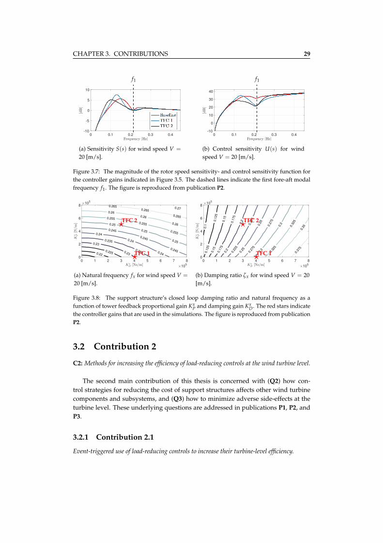
CHAPTER 3. CONTRIBUTIONS 29
0 0.1 0.2 0.3 0.4
Frequency [Hz]
-10
-5
0
5
10
[dB]
f1
(a) Sensitivity S(s) for wind speed V =
20 [m/s].
0 0.1 0.2 0.3 0.4
Frequency [Hz]
-10
0
10
20
30
40
[dB]
f1
(b) Control sensitivity U(s) for windspeed V = 20 [m/s].
Figure 3.7: The magnitude of the rotor speed sensitivity- and control sensitivity function forthe controller gains indicated in Figure 3.5. The dashed lines indicate the first fore-aft modalfrequency f1. The figure is reproduced from publication P2.
0.22
0.225
0.23
0.23
0.235
0.235
0.24
0.24
0.24
0.245
0.245
0.245
0.25
0.25
0.25
0.255
0.255
0.255
0.26
0.26
0.26
0.265
0.265
0.265
0.27
0 1 2 3 4 5 6 7 8
Kx
D[Ns/m]
×105
0
2
4
6
8
Kx P[N
/m]
×105
?
?
TFC 2
TFC 1
(a) Natural frequency fx for wind speed V =
20 [m/s].
0.1
0.1
25
0.1
25
0.1
5
0.1
5
0.1
75
0.1
75
0.2
0.2
0.2
25
0.2
25
0.2
5
0.2
5
0.2
75
0.2
75
0.3
0.3
0.3
25
0.3
25
0.3
5
0.3
75
0 1 2 3 4 5 6 7 8
Kx
D[Ns/m]
×105
0
2
4
6
8
Kx P[N
/m]
×105
?
?
TFC 2
TFC 1
(b) Damping ratio ζx for wind speed V = 20[m/s].
Figure 3.8: The support structure’s closed loop damping ratio and natural frequency as afunction of tower feedback proportional gain Kx
P and damping gain KxD. The red stars indicate
the controller gains that are used in the simulations. The figure is reproduced from publicationP2.
3.2 Contribution 2
C2: Methods for increasing the efficiency of load-reducing controls at the wind turbine level.
The second main contribution of this thesis is concerned with (Q2) how con-trol strategies for reducing the cost of support structures affects other wind turbinecomponents and subsystems, and (Q3) how to minimize adverse side-effects at theturbine level. These underlying questions are addressed in publications P1, P2, andP3.
3.2.1 Contribution 2.1
Event-triggered use of load-reducing controls to increase their turbine-level efficiency.

30 CHAPTER 3. CONTRIBUTIONS
Q1 Q2 Q3
P1 P2 P3
C1 C2 C3
Research questions
Publications
Contributions
Figure 3.9: Contribution 2.1
The potential benefits of event-triggered deployment of control strategies capa-ble of increasing the support structure’s fatigue life are analysed in publication P1.Using the mean wind speed as the triggering parameter, tradespace exploration isemployed to establish trigger criteria for near-optimal deployment of control strate-gies. The analysis considers the lifetime effect of (i) tower feedback control on thepitch bearings’ fatigue loads, (ii) tower feedback control on the main shaft’s fatigueloads, (iii) active generator torque control on the power output variability, and (iv)active generator torque control on the main shaft’s fatigue loads. As illustrated inFigure 3.10, the best choice of trigger criteria depends on the control strategy beingused and how the adversely affected components are prioritized. A near-optimaltrade-off between the support structure’s fatigue life and the pitch bearings’ fatigueloads is achieved when tower feedback control is used only in wind speeds above athreshold value. The fatigue loads in the main shaft are—opposite to the pitch bear-ings’ fatigue loads—minimized when the use of tower feedback control is restrictedto wind speeds below a threshold value. A similar divergent trend is observed foractive generator torque control. Restricting the use of active generator torque con-trol to wind speeds below a threshold value is near-optimal with regard to the poweroutput variability. With regard to the main shaft’s fatigue loads, a single trigger cri-terion does not yield a near-optimal strategy for deploying active generator torquecontrol. Fortunately, the effect on the main shaft’s fatigue loads is small comparedwith that of tower feedback control. Overall, the turbine-level efficiency of controlstrategies can be increased by adopting an event-triggered approach. This resultdoes, however, depend on the control strategy being used and the side-effect underconsideration. Nevertheless, event-triggered deployment of load-reducing controlsprovides a practical means of achieving a specific level of load-reduction at mini-mum complexity.
The effect of variations in the site-specific soil conditions on the tradespaces forevent-triggered tower feedback control are analysed in publication P2. The mag-nitude of the support structure’s responses depends on the global stiffness and the

CHAPTER 3. CONTRIBUTIONS 31
degree to which the fundamental bending mode is excited. The effects of towerfeedback control, both desirable and undesirable, are therefore sensitive to the soilconditions. The tradespaces do, however, reveal general patterns. Hence, it is rea-sonable to define a single set of trigger criteria independent of the site-specific soilconditions.
0 5 10 15 20 25 30
∆DEL20−yearβ [%]
-40
-30
-20
-10
0
∆D
20−year
Max
[%]
(a) Tradespace for the pitch actuatorbearing. The change in damage equiv-alent load for the bearing is denoted by∆DEL20-year
β .
0 2 4 6
∆DEL20−yearShaft [%]
-40
-30
-20
-10
0
∆D
20−year
Max
[%]
Trade-off scenariosVTFC ≤ V
LimTFC
VTFC ≥ VLimTFC
5
10
15
20
5
10
15
20
VLimTFC
(b) Tradespace for the main shaft. The change indamage equivalent load for the shaft is denotedby ∆DEL20-year
Shaft .
Figure 3.10: Tradespaces for event-triggered tower feedback control with mean wind speed asthe triggering parameter. ∆D20-year
Max denotes the change in fatigue utilization for the supportstructure. The stars highlight the scenarios with a single trigger criterion VLim
TFC . Red starsrepresent trigger criteria of the type VTFC ≥ VLim
TFC —meaning that tower feedback control isused for wind speeds greater than VLim
TFC —and blue stars represent trigger criteria of the typeVTFC ≤ VLim
TFC . The figure is reproduced from publication P3.
3.2.2 Contribution 2.2
Proposal and analysis of a control strategy capable of increasing the efficiency of tower feed-back control.
A tower feedback control scheme for reducing the fatigue loads in offshore windturbine support structures is proposed in publication P2. The proposed controlscheme employs collective pitch control to increase the support structure’s fore-aftdamping and stiffness. Like conventional active aerodynamic damping, tower feed-back control is implemented via an auxiliary control loop. Desirable attributes, suchas safeguarding the basic operation of the wind turbine, and straightforward integra-tion with the wind turbine’s SCADA system, are thereby maintained. The proposedcontrol scheme improves the overall efficiency of tower feedback control by (i) miti-gating undesirable interaction with the wind turbine’s basic control system, and (ii)improving the effectiveness of tower feedback control in the frequency range of thefirst-order wave loads. As explained in Section 3.1.2, the robustness and sensitiv-ity issues emerging from interaction with the rotor speed control loop are mitigated

32 CHAPTER 3. CONTRIBUTIONS
Q1 Q2 Q3
P1 P2 P3
C1 C2 C3
Research questions
Publications
Contributions
Figure 3.11: Contribution 2.2
by incorporating active tower stiffness into the tower feedback loop. This providesleeway to improve the overall performance of the two control loops. In particu-lar, it makes it possible to increase the bandwidth of the rotor speed control loopand thereby improve disturbance rejection and reduce the risk of overspeed-inducedshutdowns. With conventional active aerodynamic damping, effective tower feed-back control is restricted to a frequency range around the support structure’s firstfore-aft modal frequency. By incorporating active tower stiffness into the tower feed-back loop, effective disturbance rejection is achieved in a broader frequency rangewithout increasing the required control effort. Consequently, the trade-offs betweenthe support structure’s fatigue life and the various adverse side-effects are improved.The lifetime effects of tower feedback control with damping only (TFC 1) and damp-ing and stiffness (TFC 1+2) are presented in Table 3.4.
Table 3.4: . Lifetime effects of tower feedback control with damping only (TFC 1) and damp-ing and stiffness (TFC 1+2). In TFC 1+2, damping only is employed in below-rated operation,and damping and stiffness is employed in above-rated operation. The controller performancecomparison parameters are given in percentage [%] of operation with the basic wind turbinecontroller and desirable and undesirable effects are indicated by blue and red cells, respec-tively. The table is reproduced from publication P2.
Support structure Blade root Pitch actuators Drive-train GeneratorD20
Max D20FA D20
SS DEL20Edge DEL20
Flap DEL20β ADC20
β DEL20Gear DEL20
Shaft P20Out IAE20
ω
TFC 1 -20.0 -19.1 -12.2 -4.0 -0.9 +19.2 +103.0 +0.2 +5.5 0.0 +1.3TFC 1+2 -34.8 -34.5 -15.8 -3.9 -7.2 +21.7 +116.6 +0.2 +6.9 0.0 +1.5

CHAPTER 3. CONTRIBUTIONS 33
3.3 Contribution 3
Methods for increasing the efficiency of load-reducing controls at the wind farm level.
The third main contribution of this thesis is concerned with (Q2) how controlstrategies for reducing the cost of support structures affects other wind turbine com-ponents and subsystems, and (Q3) how to minimize adverse side-effects at the windfarm level. These underlying questions are addressed in publications P1 and P3.
3.3.1 Contribution 3.1
Methodology for turbine-specific customization of load-reducing controls to increase theirfarm-level efficiency.
Q1 Q2 Q3
P1 P2 P3
C1 C2 C3
Research questions
Publications
Contributions
Figure 3.12: Contribution 3.1
The fatigue life of individual offshore wind turbine support structures within afarm differ due to varying site conditions such as the soil conditions and the waterdepth. Since structural design of the support structures is carried out in clusters,most of them will have unused fatigue capacity at the end of their service life. Formost turbines, it is therefore unnecessary to employ control strategies for reducingthe support structure’s fatigue loads to the fullest extent possible. The applicabil-ity of turbine-specific deployment of control strategies to compensate for differingfatigue life due to varying site conditions is analysed in publication P1. By adopt-ing such an approach, it is possible to mitigate adverse side-effects at the wind farmlevel. Moreover, this approach admits the possibility of reducing the number ofclusters and thereby the number of customized support structure designs. The con-sidered sources of site variability are (i) soil conditions affecting the global stiffness,and (ii) water depth affecting the hydrodynamic loading and the global stiffness.Figure 3.13 presents the circumferential distribution of the support structure’s max-imum fatigue utilization for two cases of varying site conditions. Tower feedback
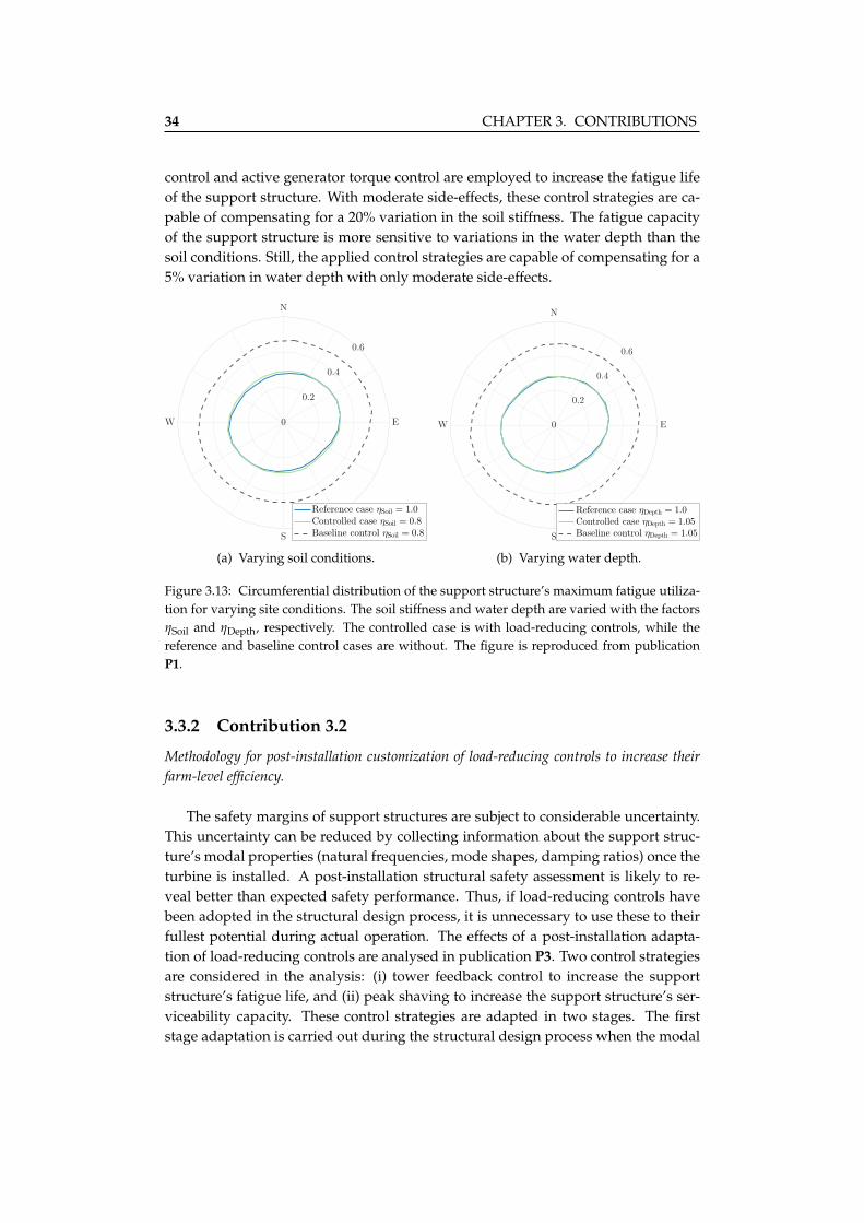
34 CHAPTER 3. CONTRIBUTIONS
control and active generator torque control are employed to increase the fatigue lifeof the support structure. With moderate side-effects, these control strategies are ca-pable of compensating for a 20% variation in the soil stiffness. The fatigue capacityof the support structure is more sensitive to variations in the water depth than thesoil conditions. Still, the applied control strategies are capable of compensating for a5% variation in water depth with only moderate side-effects.
N
E
S
W 0
0.2
0.4
0.6
Reference case ηSoil = 1.0
Controlled case ηSoil = 0.8
Baseline control ηSoil = 0.8
(a) Varying soil conditions.
N
E
S
W 0
0.2
0.4
0.6
Reference case ηDepth = 1.0
Controlled case ηDepth = 1.05
Baseline control ηDepth = 1.05
(b) Varying water depth.
Figure 3.13: Circumferential distribution of the support structure’s maximum fatigue utiliza-tion for varying site conditions. The soil stiffness and water depth are varied with the factorsηSoil and ηDepth, respectively. The controlled case is with load-reducing controls, while thereference and baseline control cases are without. The figure is reproduced from publicationP1.
3.3.2 Contribution 3.2
Methodology for post-installation customization of load-reducing controls to increase theirfarm-level efficiency.
The safety margins of support structures are subject to considerable uncertainty.This uncertainty can be reduced by collecting information about the support struc-ture’s modal properties (natural frequencies, mode shapes, damping ratios) once theturbine is installed. A post-installation structural safety assessment is likely to re-veal better than expected safety performance. Thus, if load-reducing controls havebeen adopted in the structural design process, it is unnecessary to use these to theirfullest potential during actual operation. The effects of a post-installation adapta-tion of load-reducing controls are analysed in publication P3. Two control strategiesare considered in the analysis: (i) tower feedback control to increase the supportstructure’s fatigue life, and (ii) peak shaving to increase the support structure’s ser-viceability capacity. These control strategies are adapted in two stages. The firststage adaptation is carried out during the structural design process when the modal

CHAPTER 3. CONTRIBUTIONS 35
Q1 Q2 Q3
P1 P2 P3
C1 C2 C3
Research questions
Publications
Contributions
Figure 3.14: Contribution 3.2
properties are uncertain. In this stage, the adopted control strategies are used totheir fullest potential. Once the turbine is installed, the second stage controls adap-tation is carried out under the assumption that the true modal properties are knownwith some degree of certainty. In this stage, the use of load-reducing controls areminimized as much as possible without volating structural safety requirements. Theprobabilistic outcome of a two-stage adaptation of tower feedback control and peakshaving are given in Tables 3.5 and 3.6, respectively. On average, the two-stage con-trols adaptation reduces the adverse side-effects of the adopted control strategies byup to an order of magnitude.
Table 3.5: The probabilistic outcome of a two-stage adaptation of tower feedback con-trol to increase the support structure’s fatigue life. The average change in damage equiv-
alent loads for the pitch actuator bearings and main shaft are denoted as ∆DEL20-yearβ and
∆DEL20-yearShaft , respectively. The probability of the maximum fatigue utilization being exceeded
P[D20-year
Max > 1.0]
is the probability of failure. The results are generated from 10000 randomfield (soil profile) realizations. The table is reproduced from publication P3.
Case description ∆DEL20-yearβ [%] ∆DEL20-year
Shaft [%] P[D20-year
Max > 1.0]
[%]
Basic control 0.0 0.0 5.0Conventional one-stage adaptation 22.1 6.2 5.0Two-stage adaptation η = 0.0 3.0 2.3 5.0Two-stage adaptation η = 0.5 8.8 4.4 6.2Two-stage adaptation η = 1.0 15.1 5.4 6.2

36 CHAPTER 3. CONTRIBUTIONS
Table 3.6: The probabilistic outcome of a two-stage adaptation of peak shaving to increase thesupport structure’s serviceability capacity. The average change in the lifetime energy yieldis denoted as ∆P20-year
Out and the probability of the maximum serviceability utilization being
exceeded P[θ
1-yearRated > 1.0
]is the probability of failure. The results are generated from 10000
random field (soil profile) realizations. The table is reproduced from publication P3.
Case description ∆P20-yearOut [%] P
[θ
1-yearRated > 1.0
][%]
Basic control 0.0 5.0Conventional one-stage adaptation -2.1 5.0Two-stage adaptation η = 0.0 -0.2 5.0Two-stage adaptation η = 0.5 -0.8 5.5Two-stage adaptation η = 1.0 -1.4 5.5
Chapter 4
Conclusions and Suggestionsfor Future Work
In the following chapter, the thesis is concluded and some suggestions for futurework are given.
4.1 Conclusions
The overall objective of this thesis was to develop methods for using the wind tur-bines’ control system to make their support structures more economical. The fo-cus was on the current and coming generation of wind turbines in the double-digitmegawatt range supported by large-diameter monopile foundations. The methodsdeveloped in this thesis were all based on the use of control strategies aimed at re-ducing the load effects in support structures. While such control strategies are usefulfor reducing the cost of support structures, they unavoidably produce side-effectswhich may reduce or offset potential cost savings. Hence, a major focus of this thesiswas to increase the efficiency of load-reducing controls in terms of the amount ofside-effects they produced. Two general approaches were adopted to increase theefficiency of the control strategies. The first approach was to optimize the trade-off between load reduction and adverse side-effects at the turbine level. This wasachieved by either improving the effectiveness of control strategies or through theadoption of event-triggered deployment of load-reducing controls. The second ap-proach was to reduce adverse side-effects at the wind farm level by turbine-specificadaptation of control strategies. All of the work presented in this thesis was carriedout in the context of a 10MW monopile-supported reference wind turbine located atthe Dogger Bank in the North Sea. The majority of the results were obtained fromaero-hydro-servo-elastic simulations. Some control theoretic results were obtainedfrom a reduced-order offshore wind turbine model.
An analysis of the lifetime effects of control strategies capable of increasing thesupport structure’s fatigue life gave results that were largely in line with those of
37

38CHAPTER 4. CONCLUSIONS AND SUGGESTIONS
FOR FUTURE WORK
previous studies. It was possible to significantly increase the fatigue life of sup-port structures, but at the expense of a number of adverse side-effects. Significantside-effects included power fluctuations and increased wear of the pitch system anddrive-train module. Having identified the primary side-effects, the trade-offs asso-ciated with the different control strategies were examined in the context of event-triggered deployment of load-reducing controls. It was found that the turbine-levelefficiency of control strategies could be increased by adopting such an approach.However, this result depended on the control strategy being used and the side-effectunder consideration.
Reducing structural responses by means of collective pitch control—frequentlyreferred to as tower feedback control—was by a wide margin the most effective strat-egy for increasing the fatigue life of support structures. It did, however, have severalshortcomings, including undesirable coupling with the wind turbine’s basic controlsystem and a limited frequency range of effectiveness. It was found that these short-comings could be mitigated by incorporating a proportional term (stiffness) into thetower feedback loop. This result had two main implications. First, by increasingits frequency range of effectiveness, it was possible to significantly increase the effi-ciency of tower feedback control. Second, by reducing undesirable coupling effects,tower feedback control could be used while still maintaining the bandwidth of therotor speed control loop. This was a particularly important finding as it suggeststhat tighter control of the rotor speed can be achieved without reducing the fatiguelife of the support structure.
Support structures should ideally be optimised for their specific location in thewind farm. In practice, however, they are grouped into clusters and designed forthe turbine locations giving the highest load effects. Consequently, the majority ofsupport structures are expected to have unused fatigue capacity at the end of theirservice life. It was found that turbine-specific adaptation of load-reducing controlscan be effective in equalizing the fatigue life of support structures across a windfarm. This result had three main implications. First, by reducing structural safetymargins at the wind farm level, the cost of support structures is reduced. Second,since the use load-reducing controls are isolated to design-driving turbine locations,their associated side-effects are reduced at the wind farm level. Third, the proposedmethodology could be used to increase the size of design clusters and thereby reducethe number of customized support structure designs.
There is considerable uncertainty regarding the true safety margins of supportstructures. The emergence of reliable monitoring systems has enabled the collectionof post-installation structural health data. Since design standards require conser-vative design margins, structural health monitoring is likely to reveal better thanexpected structural safety performance. Thus, if load-reducing controls have beenadopted in the structural design process, it will be concluded that it is unnecessaryto use these to their fullest potential during actual operation. Monte Carlo anal-ysis showed that, for the majority of turbines, a post-installation structural safetyassessment would reveal a significant reduction in the need for load-reducing con-

CHAPTER 4. CONCLUSIONS AND SUGGESTIONSFOR FUTURE WORK 39
trols. This result had three main implications. First and foremost, by reducing thefarm-level incidence of load-reducing controls, side-effects are reduced by up to anorder of magnitude. Second, since the post-installation controls adaptation serves asa buffer against uncertainties in the structural design process, desing conservatismis reduced at the wind farm level. Third, the significant reduction in side-effectscould enable the use of control strategies that were previously not economically vi-able. It would at least enable using load-reducing controls to a fuller extent of theircapabilities.
4.2 Suggestions for future work
While load-reducing controls have been a topic of research for many years, there isstill a general potential for developing control strategies that are capable of target-ing a wider range of load effects. Furthermore, up until now, the incorporation ofload-reducing controls into the wind farm development process has been largely un-addressed. A few suggestions for possible extensions of the present work are givenbelow.
• Control strategies for reducing ultimate load effectsUltimate strength requirements are design-driving with respect to the foun-dation embedment depth, grouted or flanged connections, and possibly somesegments near the tower top (Seidel et al., 2016). Moreover, ultimate strengthrequirements might become more important as larger-sized turbines are intro-duced. The ultimate requirements are generally stricter than requirements re-garding serviceability and fatigue life. Using control strategies for reducing ul-timate load effects therefore requires more careful consideration of the supportstructure’s safety. In addition to developing control strategies that are capableof targeting ultimate load effects, it is necessary to develop structural reliabilitymethods that are capable of handling the use of these control strategies. Onepossibility would be to use the extended contour-line method of Winterstein(2017) for taking into account multiple sub-populations of dynamic responsecharacteristics.
• Control strategies for reducing serviceability load effectsThe present work explored the possibility of using peak shaving to increasethe support structure’s serviceability capacity by reducing the maximum peakpile rotation. Evaluating the maximum pile rotation under peak loading condi-tions is a common and conservative approach. In reality, however, the designstandards require the determination of the maximum permanent accumulatedpile rotation which typically occurs under storm loading conditions. Althoughthere are currently no guidelines available on how to determine the perma-nent accumulated pile rotation, research is underway to develop a consensuson how to perform such analyses (Carswell et al., 2016). These advances call

40CHAPTER 4. CONCLUSIONS AND SUGGESTIONS
FOR FUTURE WORK
for the development of new control strategies that are capable of targeting per-manent accumulated pile rotation.
• High-fidelity assessment of the side-effects of load-reducing controlsIn order to reduce the computational effort, a reduced set of environmentalload cases was considered in the present work. While these environmental loadcases give a reasonable estimate of the support structure’s fatigue life, they donot necessarily yield accurate results for other wind turbine components. Ex-tensive simulations have provided some confidence in the results. Still, there isa need for a systematic study into the effect of reducing the number of environ-mental load cases. One possibility would be to perform a probabilistic analysisusing a joint distribution model such as the one proposed by Horn et al. (2018).
• Support structure optimizationNo effort has been made in the present work to translate the reduction in loadeffects into savings in terms of support structure weight. Such an optimiza-tion study would require repetitive simulation of design-driving loading con-ditions, and might therefore be computationally expensive. Fischer et al. (2012)proposed an optimization framework for determining the wall thickness of thesupport structure. More recently, Arany et al. (2017) have proposed a proce-dure for determining all of the support structure’s main dimensions (embed-ment length, diameter, wall thickness). Support structure optimization doesnot necessarily require the use of such an extensive procedure, but the mostcritical loading conditions should be considered.

Bibliography
Arany, L., Bhattacharya, S., Macdonald, J., and Hogan, S. (2017). Design of monopiles foroffshore wind turbines in 10 steps. Soil Dynamics and Earthquake Engineering, 92:126–152.
Arany, L., Bhattacharya, S., Macdonald, J., and Hogan, S. J. (2015a). Simplified critical mud-line bending moment spectra of offshore wind turbine support structures. Wind Energy,18(12):2171–2197.
Arany, L., Bhattacharya, S., Macdonald, J. H., and Hogan, S. J. (2016). Closed form solution ofeigen frequency of monopile supported offshore wind turbines in deeper waters incorpo-rating stiffness of substructure and ssi. Soil Dynamics and Earthquake Engineering, 83:18–32.
Arany, L., Bhattacharya, S., Macdonald, J. H., Hogan, S. J., et al. (2015b). A critical review ofserviceability limit state requirements for monopile foundations of offshore wind turbines.In Offshore Technology Conference. Offshore Technology Conference.
Bachynski, E. E. (2014). Design and dynamic analysis of tension leg platform wind turbines.
Bailey, B. H., McDonald, S. L., Bernadett, D., Markus, M., and Elsholz, K. (1997). Wind re-source assessment handbook: Fundamentals for conducting a successful monitoring pro-gram. Technical report, National Renewable Energy Lab., Golden, CO (US); AWS Scientific,Inc., Albany, NY (US).
Bak, C., Zahle, F., Bitsche, R., Kim, T., Yde, A., Henriksen, L. C., Hansen, M. H., Blasques, J. P.A. A., Gaunaa, M., and Natarajan, A. (2013). The DTU 10-MW reference wind turbine. InDanish Wind Power Research 2013.
Bhattacharya, S. (2014). Challenges in design of foundations for offshore wind turbines. Engi-neering & Technology Reference, 1(1):922.
BNEF (2016). New energy outlook 2016. Bloomberg New Energy Finance (BNEF), New York.
Bossanyi, E. (2003). Wind turbine control for load reduction. Wind energy, 6(3):229–244.
Bossanyi, E. and Witcher, D. (2009). Controller for 5MW reference turbine. European UpwindProject Report.
Brower, M. (2012). Wind resource assessment: a practical guide to developing a wind project. JohnWiley & Sons.
41

42 BIBLIOGRAPHY
Buhl, Jr, M., Wright, A., and Pierce, K. (2000). Wind turbine design codes-a comparison of thestructural response. In 2000 ASME Wind Energy Symposium, page 22.
Burton, T., Jenkins, N., Sharpe, D., and Bossanyi, E. (2011). Wind energy handbook. John Wiley& Sons.
Carswell, W., Arwade, S., DeGroot, D., and Myers, A. (2016). Natural frequency degradationand permanent accumulated rotation for offshore wind turbine monopiles in clay. Renew-able Energy, 97:319–330.
Catapult, O. R. E. (2015). Cost reduction monitoring framework summary report. OffshoreRenewable Energy Catapult, Blyth, UK.
Cole, W. J., Hand, M., Eberle, A., Beiter, P. C., Kurup, P., Turchi, C. S., Feldman, D. J., Margolis,R. M., Augustine, C. R., Maness, M., et al. (2018). 2017 annual technology baseline. Technicalreport, National Renewable Energy Lab.(NREL), Golden, CO (United States).
Damgaard, M., Bayat, M., Andersen, L. V., and Ibsen, L. B. (2014). Assessment of the dynamicbehaviour of saturated soil subjected to cyclic loading from offshore monopile wind turbinefoundations. Computers and Geotechnics, 61:116–126.
Damgaard, M., Ibsen, L. B., Andersen, L. V., and Andersen, J. K. (2013). Cross-wind modalproperties of offshore wind turbines identified by full scale testing. Journal of Wind Engi-neering and Industrial Aerodynamics, 116:94–108.
DNV GL OS-J101 (2013). Design of offshore wind turbine structures. DNV GL, Høvik, Norway.
DNV GL RP-C205 (2014). Enviromental conditions and enviromental loads . DNV GL, Høvik,Norway.
DNV GL ST-0437 (2016). Loads and site conditions for offshore wind turbines. DNV GL, Høvik,Norway.
Faltinsen, O. (1993). Sea loads on ships and offshore structures, volume 1. Cambridge universitypress.
Fischer, T., Vries, W., Rainey, P., Schmidt, B., Argyriadis, K., and Kuhn, M. (2012). Offshoresupport structure optimization by means of integrated design and controls. Wind Energy,15(1):99–117.
Fischer, T. A. (2012). Mitigation of aerodynamic and hydrodynamic induced loads of offshore windturbines. Shaker. University of Stuttgart.
Glauert, H. (1935). Airplane propellers. In Aerodynamic theory, pages 169–360. Springer.
Hamre, L., Khankandi, S., Strøm, P., and Athanasiu, C. (2011). Lateral behaviour of largediameter monopiles at sheringham shoal wind farm. Frontiers in offshore geotechnics II, pages575–580.
Hansen, M. H. and Henriksen, L. C. (2013). Basic DTU wind energy controller.
Hansen, M. O. L., Sørensen, J. N., Voutsinas, S., Sørensen, N., and Madsen, H. A. (2006). Stateof the art in wind turbine aerodynamics and aeroelasticity. Progress in aerospace sciences,42(4):285–330.

BIBLIOGRAPHY 43
Horn, J.-T., Bitner-Gregersen, E., Krokstad, J. R., Leira, B. J., and Amdahl, J. (2018). A newcombination of conditional environmental distributions. Applied Ocean Research, 73:17–26.
IEC 61400-1 (2005). Wind turbines–part 1: Design requirements. Design standard.
IEC 61400-3 (2009). Wind turbines–part 3: Design requirements for offshore wind turbines.Design standard.
IRENA (2017). Renewable power generation costs in 2017. International Renewable EnergyAgency (IRENA), Abu Dhabi.
Jonkman, J., Butterfield, S., Musial, W., and Scott, G. (2009). Definition of a 5-mw refer-ence wind turbine for offshore system development. National Renewable Energy Laboratory,Golden, CO, Technical Report No. NREL/TP-500-38060.
Jonkman, J. and Musial, W. (2010). Offshore code comparison collaboration (oc3) for iea windtask 23 offshore wind technology and deployment. Technical report, National RenewableEnergy Lab.(NREL), Golden, CO (United States).
Kallehave, D., Byrne, B. W., Thilsted, C. L., and Mikkelsen, K. K. (2015). Optimization ofmonopiles for offshore wind turbines. Phil. Trans. R. Soc. A, 373(2035):20140100.
Lazard, N. (2017). Lazards levelized cost of energy analysis–version 11.0.
Licari, J., Ekanayake, J. B., and Jenkins, N. (2013). Investigation of a speed exclusion zone toprevent tower resonance in variable-speed wind turbines. IEEE Transactions on SustainableEnergy, 4(4):977–984.
Lombardi, D., Bhattacharya, S., and Wood, D. M. (2013). Dynamic soil–structure interactionof monopile supported wind turbines in cohesive soil. Soil Dynamics and Earthquake Engi-neering, 49:165–180.
MacCamy, R. and Fuchs, R. A. (1954). Wave forces on piles: a diffraction theory. Technicalreport, CORPS OF ENGINEERS WASHINGTON DC BEACH EROSION BOARD.
Milborrow, D. (2018). At the tipping point: 2017 wind cost analysis. Windpower Monthly,34(2):18–25.
Moriarty, P. J. and Hansen, A. C. (2005). AeroDyn theory manual. National Renewable EnergyLaboratory Golden, CO.
Negro, V., Lopez-Gutierrez, J.-S., Esteban, M. D., Alberdi, P., Imaz, M., and Serraclara, J.-M. (2017). Monopiles in offshore wind: Preliminary estimate of main dimensions. OceanEngineering, 133:253–261.
Perley, T. F., Busbey, B. C., and Gerber, B. S. (2013). System and methods for determining pitchangles for a wind turbine during peak shaving. US Patent App. 13/359,837.
Peters, D. A. and He, C. J. (1991). Correlation of measured induced velocities with a finite-statewake model. Journal of the American Helicopter Society, 36(3):59–70.

44 BIBLIOGRAPHY
Popko, W., Huhn, M. L., Robertson, A., Jonkman, J., Wendt, F., Muller, K., Kretschmer, M.,Vorpahl, F., Hagen, T. R., Galinos, C., et al. (2018). Verification of a Numerical Model ofthe Offshore Wind Turbine From the Alpha Ventus Wind Farm Within OC5 Phase III. InASME 2018 37th International Conference on Ocean, Offshore and Arctic Engineering, pagesV010T09A056–V010T09A056. American Society of Mechanical Engineers.
Popko, W., Vorpahl, F., Zuga, A., Kohlmeier, M., Jonkman, J., Robertson, A., Larsen, T. J.,Yde, A., Sætertrø, K., Okstad, K. M., et al. (2012). Offshore Code Comparison Collabo-ration Continuation (OC4), Phase 1-Results of Coupled Simulations of an Offshore WindTurbine With Jacket Support Structure. In The Twenty-second International Offshore and PolarEngineering Conference. International Society of Offshore and Polar Engineers.
Prendergast, L., Reale, C., and Gavin, K. (2018). Probabilistic examination of the change ineigenfrequencies of an offshore wind turbine under progressive scour incorporating soilspatial variability. Marine Structures, 57:87–104.
Prendergast, L. J., Gavin, K., and Doherty, P. (2015). An investigation into the effect of scouron the natural frequency of an offshore wind turbine. Ocean Engineering, 101:1–11.
Robertson, A., Jonkman, J., Vorpahl, F., Popko, W., Qvist, J., Frøyd, L., Chen, X., Azcona, J.,Uzunoglu, E., Soares, C. G., et al. (2014). Offshore code comparison collaboration continu-ation within IEA wind task 30: phase II results regarding a floating semisubmersible windsystem. In ASME 2014 33rd International Conference on Ocean, Offshore and Arctic Engineering,pages V09BT09A012–V09BT09A012. American Society of Mechanical Engineers.
Robertson, A. N., Wendt, F., Jonkman, J. M., Popko, W., Dagher, H., Gueydon, S., Qvist, J.,Vittori, F., Azcona, J., Uzunoglu, E., et al. (2017). OC5 project phase II: validation of globalloads of the DeepCwind floating semisubmersible wind turbine. Energy Procedia, 137:38–57.
Robertson, A. N., Wendt, F. F., Jonkman, J. M., Popko, W., Vorpahl, F., Stansberg, C. T., Bachyn-ski, E. E., Bayati, I., Beyer, F., de Vaal, J. B., et al. (2015). OC5 project phase I: Validation ofhydrodynamic loading on a fixed cylinder. In The Twenty-fifth International Ocean and PolarEngineering Conference. International Society of Offshore and Polar Engineers.
Seidel, M. (2010). Design of support structures for offshore wind turbines–interfaces betweenproject owner, turbine manufacturer, authorities and designer. Stahlbau, 79(9):631–636.
Seidel, M. (2014). Substructures for offshore wind turbines current trends and developments.Festschrift Peter Schaumann, pages 363–368.
Seidel, M., Voormeeren, S., and van der Steen, J.-B. (2016). State-of-the-art design processes foroffshore wind turbine support structures: Practical approaches and pitfalls during differentstages in the design process. Stahlbau, 85(9):583–590.
Smilden, E., Bachynski, E. E., and Sørensen, A. J. (2017). Key contributors to lifetime accu-mulated fatigue damage in an offshore wind turbine support structure. In ASME 201736th International Conference on Ocean, Offshore and Arctic Engineering, pages V010T09A075–V010T09A075. American Society of Mechanical Engineers.
Smilden, E. and Sørensen, A. J. (2016). Application of a speed exclusion zone algorithm on alarge 10mw offshore wind turbine. In ASME 2016 35th International Conference on Ocean, Off-shore and Arctic Engineering, pages V006T09A051–V006T09A051. American Society of Me-chanical Engineers.

BIBLIOGRAPHY 45
Smith, A., Stehly, T., and Musial, W. (2015). 2014-2015 offshore wind technologies marketreport. Technical report, National Renewable Energy Lab.(NREL), Golden, CO (UnitedStates).
Tucker, M. J. and Pitt, E. G. (2001). Waves in ocean engineering. Number Volume 5.
Van der Hooft, E., Schaak, P., and Van Engelen, T. (2003). Wind turbine control algorithms.DOWEC project-DOWEC-F1W1-EH-03-094/0, Task-3 report.
Vorpahl, F., Schwarze, H., Fischer, T., Seidel, M., and Jonkman, J. (2013). Offshore wind tur-bine environment, loads, simulation, and design. Wiley Interdisciplinary Reviews: Energy andEnvironment, 2(5):548–570.
WindEurope (2010). The European offshore wind industry–Key trends and statistics 2010.Wind Europe: Brussels, Belgium.
WindEurope (2017). The European offshore wind industry–Key trends and statistics 2017.Wind Europe: Brussels, Belgium.
Winterstein, S. R. (2017). Environmental contours: Including the effects of directionality andother sub-populations. Technical report, Technical Report August, Menlo Park, CA.
Ziegler, L., Voormeeren, S., Schafhirt, S., and Muskulus, M. (2016). Design clustering of off-shore wind turbines using probabilistic fatigue load estimation. Renewable Energy, 91:425–433.

46 BIBLIOGRAPHY

Chapter 5
Appended papers
47

Contents lists available at ScienceDirect
Marine Structures
journal homepage: www.elsevier.com/locate/marstruc
Site-specific controller design for monopile offshore wind turbines
Emil Smildena,b,∗, Erin E. Bachynskia,b, Asgeir J. Sørensena,b, Jørgen Amdahla,b
a Centre for Autonomous Marine Operations and Systems, Norwegian University of Science and Technology, Trondheim, NorwaybDepartment of Marine Technology, Norwegian University of Science and Technology, Trondheim, Norway
A R T I C L E I N F O
Keywords:Offshore wind energyFoundation designController designSite-specific conditionsFatigue load reduction
A B S T R A C T
The fatigue life of offshore wind turbine (OWT) support structures is sensitive to variations insite-specific conditions such as the water depth and soil properties. Site condtions may varysignificantly within a wind farm, and they may change throughout the lifetime of the OWT. Thispaper analyses how control strategies for fatigue life extension can compensate for differingfatigue loads due to varying site conditions. Control strategies applicable for both power pro-duction and idling situations are analysed, and methodology to reduce undesirable side-effects isproposed. The design case is a 10MW monopile OWT located in 30m water depth at the DoggerBank in the North Sea, and results are based on time-domain simulations performed using anaero-hydro-servo-elastic simulation tool. The results show that, when all the investigated controlstrategies are utilized, a fatigue damage reduction over the 20-year lifetime of approximately 50%is possible. Furthermore, it is shown that adverse side-effects such as wear of pitch actuators andfluctuations in the power output can be significantly reduced by limiting the use of controlstrategies to some predefined situations. With only moderate cost to other system components,the control system is able to compensate for 20% variation in soil stiffness, and 5% (1.5 m) var-iation in water depth.
1. Introduction
The offshore wind industry is continuously progressing towards larger wind turbines, with the first 8MW wind turbines grid-connected in 2016 [1]. Larger wind turbines require larger support structures, which without considering the cost of installation, is acomponent that represents close to 20% of the total cost of offshore wind farms [2,3]. Monopiles remain the favoured choice offoundation with a market share of 88% in Europe [1], and this trend is expected to persist for wind turbines installed in shallow andintermediate water depths (<40 meters) [4]. Monopile dimensions are mainly driven by fatigue considerations, and the increase infatigue loads resuting from the upscaling of turbines in combination with deeper water, is a challenge for the economical feasibility ofmonopile foundations [5]. In particular, large monopiles are more susceptible to fatigue damage from first order wave loads. Themagnitude of the hydrodynamic loads increases due to the larger diameter of the monopile. Furthermore, the increased mass of therotor-nacelle assembly (RNA) and height of the wind turbine, together with a reduction of the rotor speed and the correspondingfrequency constraint imposed by the blade passing frequency (3P), pushes the first modal frequencies of the support structure closerto typical wave frequencies [6,7].
The wind turbine's blade pitch and generator torque control system influences the dynamic response of the structure. The design
https://doi.org/10.1016/j.marstruc.2018.03.002Received 1 November 2017; Received in revised form 31 January 2018; Accepted 2 March 2018
∗ Corresponding author. Centre for Autonomous Marine Operations and Systems, Norwegian University of Science and Technology, Trondheim, Norway.E-mail address: [email protected] (E. Smilden).
Abbreviations: AAD, Active aerodynamic damping; AGT, Active generator torque control; AIC, Active idling control; DEL, Damage equivalent load; DLC, Design loadcase; ELC, Environmental load case; FLS, Fatigue limit state; OWT, Offshore wind turbine; RNA, Rotor-nacelle assembly; SCO, Soft cut-out; TMD, Tuned mass damper;ULS, Ultimate limit state
Marine Structures 61 (2018) 503–523
Available online 14 July 20180951-8339/ © 2018 Elsevier Ltd. All rights reserved.
T

process for offshore wind turbines (OWTs) should therefore be carried out in an integrated manner, including the design of controlstrategies that aim to reduce fatigue loads in the support structure [5]. Monopile OWTs are lightly damped, with typical dampingratios in the range 1% - 2.5% of critical for the first fore-aft and side-side vibration modes [8–10]. Aerodynamic damping from therotor is an important contribution to the overall damping of the fore-aft vibration modes, and several control strategies that are basedon enhancing the aerodynamic damping to reduce fatigue loads have been studied [7,11–15]. Because the rotor mainly contributeswith damping in the fore-aft direction, the support structure is particularly prone to excitation by waves coming from a differentdirection than the wind. The incidence of environmental conditions with wind/wave misalignment is site-specific, but it can besignificant for exposed wind farm locations [16,17]. Several control strategies that aim to increase the damping of the side-sidevibration modes of the support structure have been proposed [7,11,13,14,18,19]. The various control strategies for fatigue loadreduction are presented in more detail in Section 2.
As demonstrated in Refs. [5,7], control strategies for fatigue load reduction can be integrated in the design process for the supportstructure, leading to a 9.2% reduction in the weight. A control system that can extend the fatigue life of the OWT can also be used tocompensate for uncertainties or simplifications in the design process. The fatigue loading of monopile OWTs is sensitive to variationsin site specific conditions such as the water depth and soil properties [20–22]. Because the water depth and soil properties may varysignificantly within a wind farm, it is common industry practice to group the OWTs into clusters, and design the support structuresaccording to the most loaded location in the cluster [23]. The conservatism of this approach may be reduced by introducing controlstrategies that can compensate for differing fatigue loads due to varying site conditions. Moreover, such control strategies may beapplied to increase the size of the design clusters, thereby reducing the number of customized foundation designs. Because the soilproperties are associated with large uncertainties [24,25], the true modal properties of the support structure, particularly the naturalfrequencies and damping ratios, are often not known before the wind turbine is installed [9]. Furthermore, long-term cyclic loadingmay cause accumulated pile displacements and changes in the soil properties, thereby changing the modal properties over thelifetime of the OWT [22]. Control strategies that extend the fatigue life of the OWT, may reduce the design conservatism resultingfrom uncertainty in the modal parameters. Moreover, one could equalize the fatigue utilization for the foundations across the windfarm such that the turbines can be decommissioned at the same time without wasting structural reserves.
Control strategies which mitigate fatigue loads in the support structure, can lead to undesirable side-effects in other wind turbinecomponents. The reliability of the pitch system is a concern with control strategies that require additional pitch activity. A surveyconsisting of 1400 turbine years of operational data for onshore variable speed turbines found the pitch system to be the sub-assemblywith the highest failure rate [26,27]. Moreover, because the pitch system reliability is difficult to predict, it is desirable to limit theuse of pitch actuators. Other critical components that may be negatively affected by the control system are the blades, main shaft,gearbox, and generator. These components have lower failure rates, but they cause higher downtimes when they fail [26]. Fur-thermore, it is essential to maintain power production, with power quality that complies with grid requirements [28]. A compromisebetween fatigue load reduction and collateral effects can be achieved by limiting the use of control strategies to certain predefinedsituations. Enabling control strategies in situations where the tower-top vibration frequency is within a frequency band containingthe first modal frequency of the support structure was proposed by Refs. [29,30]. Further [3,31], proposed enabling control strategiesbased on information about environmental conditions, and a multi-objective optimization method was developed to establish thetrigger criteria.
The main contribution of the present work is the analysis of the applicability of control strategies for fatigue load reduction tocompensate for differing fatigue loads due to varying site conditions. As such, only the fatigue limit state (FLS) is considered, not theultimate limit state (ULS) and serviceability limit state (SLS). This paper also demonstrates the long-term effects of control strategiesfor fatigue load reduction. A similar study was performed by Ref. [7] for a 5MW OWT. In this paper, a 10MW OWT is considered, andby comparing the results, the present work serves as a verification and extension of previous research. Furthermore, this paperanalyses the trade-offs between fatigue load reduction and undesirable side-effects, and proposes a methodology to improve theoverall trade-offs associated with the control strategies. The simulation model is based on the 10MW reference wind turbine of DTUWind Energy [32], and long-term variations in environmental conditions are based on 60 years of hindcast data for a wind farm siteat the Dogger Bank in the North Sea [33]. Simulations are performed using the software tool SIMA by SINTEF Ocean with post-processing in MATLAB by aid of the WAFO toolbox [34].
The paper is organized as follows: In Sec. 2, an overview of control strategies for fatigue load reduction is given, and the studiedcontrol strategies are presented in detail. In Sec. 3, the simulation setup is described, and controller performance parameters areestablished. In Sec. 4, the simulation results are presented and discussed. First, the baseline design case is evaluated, and the long-term effects of control strategies are assessed. Next, the trade-offs between fatigue load reduction and undesirable side-effects areinvestigated, and methodology to improve the overall performance is developed. Finally, applicability of control system design tocompensate for differing fatigue loads due to varying site condtions, is assessed. The paper is concluded in Sec. 5.
2. Control concepts for fatigue load reduction
2.1. Overview of control strategies
Wind turbines harvest energy between a cut-in wind speed (typical =V 4In [m/s]) and a cut-out wind speed ( =V 25Out [m/s])[35]. Depending on the wind speed, the wind turbine control system operates in one of two modes. For wind speeds below the rated
E. Smilden et al. Marine Structures 61 (2018) 503–523
504
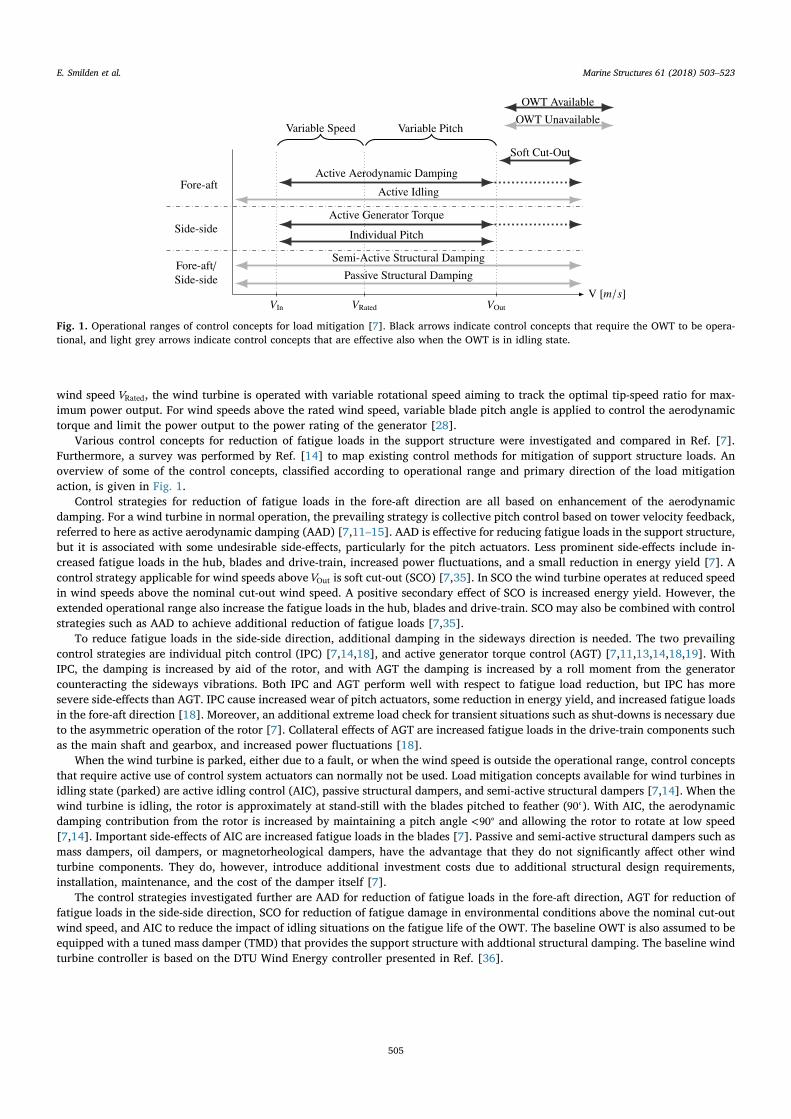
wind speed VRated, the wind turbine is operated with variable rotational speed aiming to track the optimal tip-speed ratio for max-imum power output. For wind speeds above the rated wind speed, variable blade pitch angle is applied to control the aerodynamictorque and limit the power output to the power rating of the generator [28].
Various control concepts for reduction of fatigue loads in the support structure were investigated and compared in Ref. [7].Furthermore, a survey was performed by Ref. [14] to map existing control methods for mitigation of support structure loads. Anoverview of some of the control concepts, classified according to operational range and primary direction of the load mitigationaction, is given in Fig. 1.
Control strategies for reduction of fatigue loads in the fore-aft direction are all based on enhancement of the aerodynamicdamping. For a wind turbine in normal operation, the prevailing strategy is collective pitch control based on tower velocity feedback,referred to here as active aerodynamic damping (AAD) [7,11–15]. AAD is effective for reducing fatigue loads in the support structure,but it is associated with some undesirable side-effects, particularly for the pitch actuators. Less prominent side-effects include in-creased fatigue loads in the hub, blades and drive-train, increased power fluctuations, and a small reduction in energy yield [7]. Acontrol strategy applicable for wind speeds above VOut is soft cut-out (SCO) [7,35]. In SCO the wind turbine operates at reduced speedin wind speeds above the nominal cut-out wind speed. A positive secondary effect of SCO is increased energy yield. However, theextended operational range also increase the fatigue loads in the hub, blades and drive-train. SCO may also be combined with controlstrategies such as AAD to achieve additional reduction of fatigue loads [7,35].
To reduce fatigue loads in the side-side direction, additional damping in the sideways direction is needed. The two prevailingcontrol strategies are individual pitch control (IPC) [7,14,18], and active generator torque control (AGT) [7,11,13,14,18,19]. WithIPC, the damping is increased by aid of the rotor, and with AGT the damping is increased by a roll moment from the generatorcounteracting the sideways vibrations. Both IPC and AGT perform well with respect to fatigue load reduction, but IPC has moresevere side-effects than AGT. IPC cause increased wear of pitch actuators, some reduction in energy yield, and increased fatigue loadsin the fore-aft direction [18]. Moreover, an additional extreme load check for transient situations such as shut-downs is necessary dueto the asymmetric operation of the rotor [7]. Collateral effects of AGT are increased fatigue loads in the drive-train components suchas the main shaft and gearbox, and increased power fluctuations [18].
When the wind turbine is parked, either due to a fault, or when the wind speed is outside the operational range, control conceptsthat require active use of control system actuators can normally not be used. Load mitigation concepts available for wind turbines inidling state (parked) are active idling control (AIC), passive structural dampers, and semi-active structural dampers [7,14]. When thewind turbine is idling, the rotor is approximately at stand-still with the blades pitched to feather ( ∘90 ). With AIC, the aerodynamicdamping contribution from the rotor is increased by maintaining a pitch angle < ∘90 and allowing the rotor to rotate at low speed[7,14]. Important side-effects of AIC are increased fatigue loads in the blades [7]. Passive and semi-active structural dampers such asmass dampers, oil dampers, or magnetorheological dampers, have the advantage that they do not significantly affect other windturbine components. They do, however, introduce additional investment costs due to additional structural design requirements,installation, maintenance, and the cost of the damper itself [7].
The control strategies investigated further are AAD for reduction of fatigue loads in the fore-aft direction, AGT for reduction offatigue loads in the side-side direction, SCO for reduction of fatigue damage in environmental conditions above the nominal cut-outwind speed, and AIC to reduce the impact of idling situations on the fatigue life of the OWT. The baseline OWT is also assumed to beequipped with a tuned mass damper (TMD) that provides the support structure with addtional structural damping. The baseline windturbine controller is based on the DTU Wind Energy controller presented in Ref. [36].
Fig. 1. Operational ranges of control concepts for load mitigation [7]. Black arrows indicate control concepts that require the OWT to be opera-tional, and light grey arrows indicate control concepts that are effective also when the OWT is in idling state.
E. Smilden et al. Marine Structures 61 (2018) 503–523
505
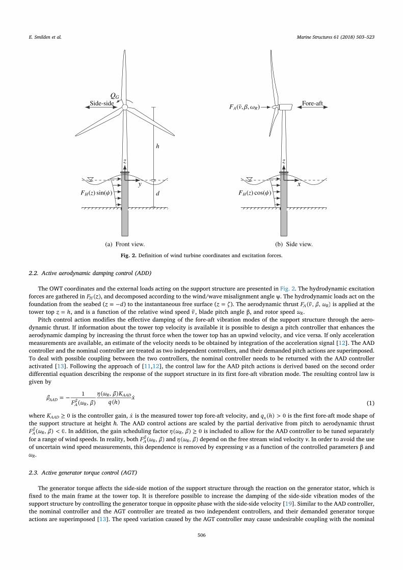
2.2. Active aerodynamic damping control (ADD)
The OWT coordinates and the external loads acting on the support structure are presented in Fig. 2. The hydrodynamic excitationforces are gathered in F z( )H , and decomposed according to the wind/wave misalignment angle ψ. The hydrodynamic loads act on thefoundation from the seabed ( = −z d) to the instantaneous free surface ( =z ζ ). The aerodynamic thrust F v β ω( , , )A R is applied at thetower top =z h, and is a function of the relative wind speed v , blade pitch angle β, and rotor speed ωR.
Pitch control action modifies the effective damping of the fore-aft vibration modes of the support structure through the aero-dynamic thrust. If information about the tower top velocity is available it is possible to design a pitch controller that enhances theaerodynamic damping by increasing the thrust force when the tower top has an upwind velocity, and vice versa. If only accelerationmeasurements are available, an estimate of the velocity needs to be obtained by integration of the acceleration signal [12]. The AADcontroller and the nominal controller are treated as two independent controllers, and their demanded pitch actions are superimposed.To deal with possible coupling between the two controllers, the nominal controller needs to be returned with the AAD controlleractivated [13]. Following the approach of [11,12], the control law for the AAD pitch actions is derived based on the second orderdifferential equation describing the response of the support structure in its first fore-aft vibration mode. The resulting control law isgiven by
= −βF ω β
η ω β Kq h
x1( , )
( , )( )
˙AADAβ
R
R AAD
(1)
where ≥K 0AAD is the controller gain, x is the measured tower top fore-aft velocity, and >q h( ) 0x is the first fore-aft mode shape ofthe support structure at height h. The AAD control actions are scaled by the partial derivative from pitch to aerodynamic thrust
<F ω β( , ) 0Aβ
R . In addition, the gain scheduling factor ≥η ω β( , ) 0R is included to allow for the AAD controller to be tuned separatelyfor a range of wind speeds. In reality, both F ω β( , )A
βR and η ω β( , )R depend on the free stream wind velocity v. In order to avoid the use
of uncertain wind speed measurements, this dependence is removed by expressing v as a function of the controlled parameters β andωR.
2.3. Active generator torque control (AGT)
The generator torque affects the side-side motion of the support structure through the reaction on the generator stator, which isfixed to the main frame at the tower top. It is therefore possible to increase the damping of the side-side vibration modes of thesupport structure by controlling the generator torque in opposite phase with the side-side velocity [19]. Similar to the AAD controller,the nominal controller and the AGT controller are treated as two independent controllers, and their demanded generator torqueactions are superimposed [13]. The speed variation caused by the AGT controller may cause undesirable coupling with the nominal
Fig. 2. Definition of wind turbine coordinates and excitation forces.
E. Smilden et al. Marine Structures 61 (2018) 503–523
506
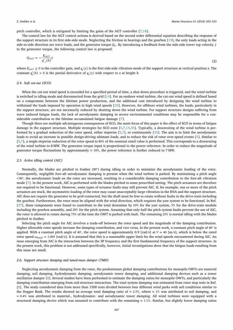
pitch controller, which is mitigated by limiting the gains of the AGT controller [7,18].The control law for the AGT control actions is derived based on the second order differential equation describing the response of
the support structure in its first side-side mode. Neglecting the friction in bearings and the gearbox [19], the only loads acting in theside-to-side direction are wave loads, and the generator torque QG. By introducing a feedback from the side-side tower top velocity yto the generator torque, the following control law is proposed:
= −′
Q Kq h
y( )
˙AGTAGT
y (2)
where ≥K 0AGT is the controller gain, and q z( )y is the first side-side vibration mode of the support structure at vertical position z. Theconstant ′ >q h( ) 0y is the partial derivative of q z( )y with respect to z at height h.
2.4. Soft cut-out (SCO)
When the cut-out wind speed is exceeded for a specified period of time, a shut down procedure is triggered, and the wind turbineis switched to idling mode and disconnected from the grid [14]. For an onshore wind turbine, the cut-out wind speed is defined basedon a compromise between the lifetime power production, and the addtional cost introduced by designing the wind turbine towithstand the loads imposed by operation in high wind speeds [35]. However, for offshore wind turbines, the loads, particularly inthe support structure, are not necessarily reduced by shutting down the wind turbine. For support structure designs suffering fromwave induced fatigue loads, the lack of aerodynamic damping in severe environmental conditions may be responsible for a con-siderable contribution to the lifetime accumulated fatigue damage [7].
Though there are multiple advantageous consequences of SCO, the main focus of this paper is the effect of SCO in terms of fatiguedamage in the support structure. Multiple strategies for SCO exist [5,7,14,35]. Typically, a downrating of the wind turbine is per-formed by a gradual reduction of the rotor speed, either stepwise [5,7], or continuously [35]. The aim is to limit the aerodynamicloads to avoid an increase in possible design-driving ultimate loads, and to reduce the risk of rotor over-speed events [5]. Similar to[5,7], a single stepwise reduction of the rotor speed to 80% of the nominal rated value is performed. This corresponds to a downratingof the wind turbine to 8MW. The generator torque input is proportional to the power reference. In order to reduce the magnitude ofgenerator torque fluctuations by approximately ≈ 10%, the power reference is further reduced to 7MW.
2.5. Active idling control (AIC)
Normally, the blades are pitched to feather ( ∘90 ) during idling in order to minimize the aerodynamic loading of the rotor.Consequently, negligible fore-aft aerodynamic damping is present when the wind turbine is parked. By maintaining a pitch angle< ∘90 , the aerodynamic loads on the rotor are increased, resulting in a considerable damping contribution to the fore-aft vibrationmode [7]. In the present work, AIC is performed with the blades pitched to some prescribed setting. The pitch actuators are thereforenot required to be functional. However, some types of actuator faults may still prevent AIC. If, for example, one or more of the pitchactuators are stuck, the asymmetric loading of the rotor may cause unacceptably large vibration in the RNA and the support structure.AIC does not require the generator to be grid-connected, but the shaft must be free to rotate without faults in the drive-train includingthe gearbox. Furthermore, the rotor must be aligned with the wind direction, which requires the yaw system to be functional. In Ref.[27], these components were found to contribute to the total downtime by 10% for the yaw system, 5% for the drive-train moduleincluding the gearbox assembly, and 20% for the pitch system. Assuming that only half the pitch system faults prevent the use of AIC,the rotor is allowed to rotate during 75% of the time the OWT is parked with fault. The remaining 25% is normal idling with the bladespitched to feather.
Selecting the pitch angle for AIC involves a trade-off between the rotor speed and the magnitude of the damping contribution.Higher allowable rotor speeds increase the damping contribution, and vice versa. In the present work, a constant pitch angle of ∘40 isapplied. With a constant pitch angle of ∘40 , the rotor speed is approximately 0.9 [rad/s] at =V 40 [m/s], which is below the ratedrotor speed =ω 1.005Rated [rad/s]. It is assumed that this is a reasonable upper limit for the wind speeds encountered during AIC. Anissue emerging from AIC is the interaction between the 3P frequency and the first fundamental frequency of the support structure. Inthe present work, this problem is not addressed specifically, however, initial investigations show that the fatigue loads resulting fromthis issue are small.
2.6. Support structure damping and tuned-mass damper (TMD)
Neglecting aerodynamic damping from the rotor, the predominant global damping contributions for monopile OWTs are materialdamping, soil damping, hydrodynamic damping, aerodynamic tower damping, and additional damping devices such as a toweroscillation damper [8]. Several studies have been performed to estimate the damping ratios for monopile OWTs, and particularly thedamping contribution emerging from soil-structure interaction. The total system damping was estimated from rotor stop tests in Ref.[8]. The study considered data from more than 1500 tests divided between four different wind parks with soil conditions similar tothe Dogger Bank. The results showed an average total damping ratio of ≈ 2.5%, where ≈ 1% was attributed to soil damping, and≈ 0.4% was attributed to material-, hydrodynamic- and aerodynamic tower damping. All wind turbines were equipped with astructural damping device which was assumed to contribute with the remaining ≈ 1.1%. Similar, but slightly lower damping ratios
E. Smilden et al. Marine Structures 61 (2018) 503–523
507

were observed by Refs. [9,10], which investigated rotor stop tests performed on an offshore wind turbine placed in a location withsoil mainly consisting of sand. The structural damper was turned off during the tests, and the total damping ratio was estimated as≈ 1.0%. Furthermore [37], concluded that soil-structure interaction contributed with damping in the range 0.17% - 0.72% for soilconditions that are typical for the North Sea. Based on these results, the damping ratio for the support structure is taken as 1.1%,where 0.5% is due to material-, hydrodynamic- and aerodynamic damping, and 0.6% is due to soil damping. Two TMDs are included inthe simulation model, increasing the damping ratio for the first fore-aft and side-side vibration modes to 2.2%. The TMDs are locatedin the top of the tower, and the TMD mass is 20 tonnes, corresponding to approximately 2% of the modal mass for the first funda-mental mode. The natural frequency of the dampers are tuned to the natural frequency of the first fundamental mode, and a con-figuration with two independent dampers in the fore-aft and side-side direction is used, following [38].
3. Simulation setup
This section is organized as follows: First, a procedure for establishing an environmental design basis is presented. Next, thedesign load cases are selected according to the standard [39]. Further, the simulation model is presented, and the procedure forestimation of support structure fatigue damage is explained. Finally, the comparison parameters that will be used to assess theperformance of control strategies are established.
3.1. Environmental conditions
A wind farm site at the Dogger Bank in the North Sea is chosen as the design location. Hindcast data for a period of 60 years with aresolution of 3 h, are provided by the Norwegian Meterological Institute. Details regarding the hindcast, which covers the North Sea,the Norwegian Sea, and the Barents Sea, are found in Ref. [33]. Furthermore, a detailed statistical description of the metocean datafor the design location is given in Ref. [17], and some important features with regard to assessment of the lifetime fatigue strength arepresented in Ref. [6]. The metocean data contains information about significant wave height Hs, peak periodTp, wave direction, meanwind speed V, and wind direction. Turbulence intensity and wind shear, which were not considered in the hindcast, are accounted forin accordance with [40]. A complete assessment of the lifetime fatigue strength of the support structure should include long-termvariations in at least: Hs, Tp, V, wind direction, wave direction, and turbulence intensity. The number of environmental parameterscan be reduced to four by assuming the turbulence intensity to be a function of V, and introducing the misalignment angle ψ as therelative angle between the wind and wave direction. Even with the reduction of environmental parameters, it is computationallyimpracticable to consider all possible combinations. A procedure for lumping of environmental conditions to environmental loadcases (ELCs) is therefore developed:
Step 1 Grouping of metocean data: To reduce the number of environmental conditions, the metocean data is distributed into athree dimensional collection of bins, based on the environmental parameters V, ψ, and Hs. Starting with wind speed V, a binsize of 2 [m/s], in accordance with [39], is used. Further, the wind/wave misalignment ψ is divided into sectors of ∘30 asshown in Fig. 3, with wind always coming from ∘0 , and waves coming from ∘0 , …∘ ∘30 , ,180 [6]. Following [3], the number ofbins are halved by merging the sectors mirrored about the vertical axis. For each of the × =16 7 112 combinations of V and ψ,three sea states are considered. The resulting number of ELCs are × × =16 7 3 336. However, after removing the environ-mental conditions with occurrence probability less than × −1 10 4, the number is reduced to 138.
Fig. 3. Wind/wave misalignment bins, with wind from ∘0 and waves from ∘0 , …∘ ∘30 , ,180 . Bins with the same shade of grey are merged [3,6]. (Forinterpretation of the references to color in this figure legend, the reader is referred to the Web version of this article.)
E. Smilden et al. Marine Structures 61 (2018) 503–523
508
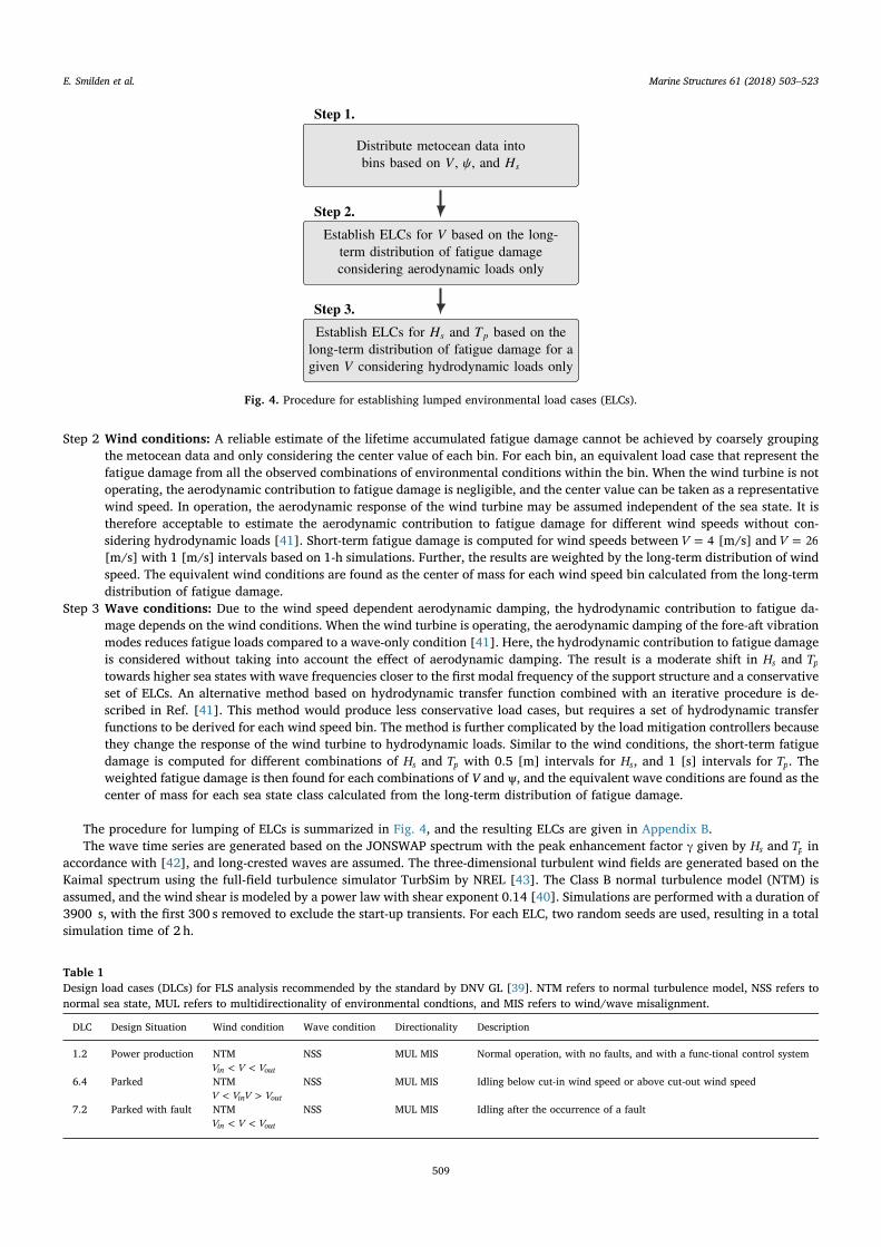
Step 2 Wind conditions: A reliable estimate of the lifetime accumulated fatigue damage cannot be achieved by coarsely groupingthe metocean data and only considering the center value of each bin. For each bin, an equivalent load case that represent thefatigue damage from all the observed combinations of environmental conditions within the bin. When the wind turbine is notoperating, the aerodynamic contribution to fatigue damage is negligible, and the center value can be taken as a representativewind speed. In operation, the aerodynamic response of the wind turbine may be assumed independent of the sea state. It istherefore acceptable to estimate the aerodynamic contribution to fatigue damage for different wind speeds without con-sidering hydrodynamic loads [41]. Short-term fatigue damage is computed for wind speeds between =V 4 [m/s] and =V 26[m/s] with 1 [m/s] intervals based on 1-h simulations. Further, the results are weighted by the long-term distribution of windspeed. The equivalent wind conditions are found as the center of mass for each wind speed bin calculated from the long-termdistribution of fatigue damage.
Step 3 Wave conditions: Due to the wind speed dependent aerodynamic damping, the hydrodynamic contribution to fatigue da-mage depends on the wind conditions. When the wind turbine is operating, the aerodynamic damping of the fore-aft vibrationmodes reduces fatigue loads compared to a wave-only condition [41]. Here, the hydrodynamic contribution to fatigue damageis considered without taking into account the effect of aerodynamic damping. The result is a moderate shift in Hs and Tptowards higher sea states with wave frequencies closer to the first modal frequency of the support structure and a conservativeset of ELCs. An alternative method based on hydrodynamic transfer function combined with an iterative procedure is de-scribed in Ref. [41]. This method would produce less conservative load cases, but requires a set of hydrodynamic transferfunctions to be derived for each wind speed bin. The method is further complicated by the load mitigation controllers becausethey change the response of the wind turbine to hydrodynamic loads. Similar to the wind conditions, the short-term fatiguedamage is computed for different combinations of Hs and Tp with 0.5 [m] intervals for Hs, and 1 [s] intervals for Tp. Theweighted fatigue damage is then found for each combinations of V and ψ, and the equivalent wave conditions are found as thecenter of mass for each sea state class calculated from the long-term distribution of fatigue damage.
The procedure for lumping of ELCs is summarized in Fig. 4, and the resulting ELCs are given in Appendix B.The wave time series are generated based on the JONSWAP spectrum with the peak enhancement factor γ given by Hs and Tp in
accordance with [42], and long-crested waves are assumed. The three-dimensional turbulent wind fields are generated based on theKaimal spectrum using the full-field turbulence simulator TurbSim by NREL [43]. The Class B normal turbulence model (NTM) isassumed, and the wind shear is modeled by a power law with shear exponent 0.14 [40]. Simulations are performed with a duration of3900 s, with the first 300 s removed to exclude the start-up transients. For each ELC, two random seeds are used, resulting in a totalsimulation time of 2 h.
Fig. 4. Procedure for establishing lumped environmental load cases (ELCs).
Table 1Design load cases (DLCs) for FLS analysis recommended by the standard by DNV GL [39]. NTM refers to normal turbulence model, NSS refers tonormal sea state, MUL refers to multidirectionality of environmental condtions, and MIS refers to wind/wave misalignment.
DLC Design Situation Wind condition Wave condition Directionality Description
1.2 Power production NTM< <V V Vin out
NSS MUL MIS Normal operation, with no faults, and with a func-tional control system
6.4 Parked NTM<V Vin >V Vout
NSS MUL MIS Idling below cut-in wind speed or above cut-out wind speed
7.2 Parked with fault NTM< <V V Vin out
NSS MUL MIS Idling after the occurrence of a fault
E. Smilden et al. Marine Structures 61 (2018) 503–523
509

3.2. Design load cases
The design load cases (DLCs) considered for calculation of the lifetime accumulated fatigue damage are given in Table 1. Si-tuations such as startup and shutdown, or occurrence of failure modes, are assumed to have small contributions to fatigue damageover the lifetime of the support structure, and design load cases concerning these situations are disregarded [7]. Furthermore, designload cases concerning operation with ice formation, and transport, installation, maintenance, and repair, are also disregarded.
In DLC 7.2 the wind turbine is idling after the occurrence of a fault. It is assumed that the availability of the wind turbine isindependent of environmental conditions, and that the total availability is 90%, following the recommendation of [39]. DLC 7.2therefore accounts for 10% of the lifetime, evenly spread over all environmental conditions. An availability ratio of 90% is a con-servative estimate, and contractual availability of 95% is common for offshore wind turbines [44].
When the wind turbine is operating (DLC 1.2), or is parked without fault (DLC 6.4), the yaw system is active. Following therecommendation of [39], yaw errors of ± ∘8 are introduced in the simulations to account for the hysteretic behaviour of the yawsystem. When the wind turbine is parked with fault (DLC 7.2) the yaw system cannot be assumed active. Due to limitations of thesimulation tool and implemented theory, large yaw misalignments give unreliable results. Yaw errors of ± ∘8 are therefore assumedalso for DLC 7.2.
3.3. Simulation model
The wind turbine is modeled in the aero-hydro-servo-elastic simulation tool SIMA by SINTEF Ocean. The structural modelcomprising the foundation, tower, and blades, is modeled using nonlinear beam elements that accounts for large deformations [4].The soil stiffness is modeled using nonlinear springs with stiffness properties computed from pressure-displacement curves. The soilprofile is based on conditions at the Dogger Bank with a 1.5 m top layer of cohesionless soil (sand) followed by cohesive soils (clay).The pressure-displacement curves are computed according to [45] using the most conservative (lowest) estimate of the clay shearstrength. The material-, hydrodynamic- and aerodynamic damping is accounted for by stiffness-proportional Rayleigh dampingdistributed along the complete support structure, and the soil damping is accounted for by increasing the Rayleigh damping in thefoundation beneath the mudline.
Aerodynamic loads are modeled using blade element momentum (BEM) theory with corrections for tip loss, hub loss, dynamicinflow, dynamic wake, skewed inflow, and tower shadow [46]. Hydrodynamic loads are calculated based on Morison's equationaccounting for relative velocities and assuming Airy linear wave theory with the wave kinematics integrated to the instantaneous freesurface [47]. In all simulations, the inertia coefficient is taken as =C 2M and the quadratic drag coefficient is taken as =C 0.9D [4].The simulation model is based on the 10MW reference wind turbine of DTU Wind Energy [32] placed on a monopile foundation withdiameter 8.5 m. The monopile is placed in 30m water depth, and the total depth of the monopile is 42m below the seabed. The windturbine tower is stiffened compared to the tower in Ref. [32] through a 20 % increase in wall thickness [4]. The first modal fre-quencies of the support structure are 0.214 Hz for the fore-aft mode, and 0.213 Hz for the side-side mode.
3.4. Support structure fatigue calculation
The lifetime accumulated fatigue damage is computed by combining short-term estimates of fatigue damage with the long-termvariations in environmental conditions. The short-term fatigue damage is calculated based on rainflow counting of stress cycleamplitudes [48], and summation of fatigue damage based on the S-N approach following the Palmgren-Miner linear damage hy-pothesis. The short-term time histories of stress in the support structure are computed from time histories of bending moments andinternal forces obtained from SIMA. Only the fatigue contribution from axial stress is considered. The post processing of stresshistories is performed in MATLAB using the WAFO implementation [34] of rainflow counting, the S-N method and Palmgren-Minersummation modified to account for a bi-linear S-N curve.
The S-N curve recommended by Ref. [49] for steel in water with cathodic protection is applied. Because fatigue damage is likelyto occur in weld details rather than in the base material, detail category D is used [4]. The applied S-N curve is bi-linear withexponent 5 for high-cycle fatigue and exponent 3 for low-cycle fatigue. Stress calculations are performed with a stress concentrationfactor of 1. Higher stress concentration factors may be applicable for some sections of the support structure such as the tower top, theintersection between the tower and the transition piece, or at the mudline. This is, however, disregarded for simplicity, since the focusis on comparison of control strategies. Locations along the support structure that are critical with regard to fatigue strength are thefoundation beneath the mudline, and in the intersection between the tower and the transition piece [4,6,7]. It is required by Ref. [50]to use a safety factor of 3 for non-accessible areas, which applies for the foundation, but not the tower. Based on initial investigations,the foundation is taken as the critical component with regard to fatigue failure. The cross-section 6m below the mudline was found tohave the highest fatigue utilization.
3.5. Performance comparison parameters
Several representative parameters related to different wind turbine components are used to evaluate the performance of the loadmitigation strategies. All performance parameters are presented by comparison with the baseline case, expressed in percentage. Theperformance comparison parameters and their desired trend are summarized in Table 2. For all components it is desirable to limit theincrease in performance parameters as much as possible, except from the power output. Because the actual fatigue utilization of the
E. Smilden et al. Marine Structures 61 (2018) 503–523
510

foundation is estimated, and a bi-linear S-N curve is applied for the fatigue calculations, fatigue damage (D) is used as performancemeasure for the support structure. For the other components, damage equivalent load (DEL) is used. It is stressed that changes in Dand DEL are scaled differently. For a given S-N slope exponent p, the relationship between a change in fatigue damage DΔ and fatigueload Δ DEL is given by
= DΔDEL Δ p1 (3)
The maximum 20-year accumulated fatigue damage (Dmax20 ) in the critical foundation cross-section, is taken as the primary
measure of control strategy performance in terms of support structure fatigue damage. In addition, the 20-year accumulated fatiguedamage in the fore-aft direction (DFA
20 ) and the side-side direction (DSS20) in the critical cross-section, is computed to investigate how
the control strategies affect the fore-aft and side-side vibration modes. Wind speed directionality is disregarded from the analysis inorder to compute DFA
20 and DSS20 (only the relative wave direction is considered). The full lifetime fatigue damage considers both effects
around the full circumference of the foundation.Further, the blade root fatigue loads are considered. The flapwise and edgewise lifetime weighted damage equivalent load,
denoted as DELEdge20 and DELFlap
20 , are computed from the time histories of blade root bending moments. The long-term DEL for a load Sover k number of ELCs is calculated according to
⎜ ⎟⎛⎝
∑ ∑ ⎞⎠
∝ P i S nDEL [ ]i
k
j
n
jp
j
p20
1i
(4)
where p is the slope of the S-N curve, nj is the number of load cycles at load range Sj [48], and ni is the number of load ranges for ELC iwith probability P i[ ]. Because only the relative value compared with the baseline case is used, all constants are ommited from theexpression in Eq. (4). The number of load cycles per load range is determined by use of rainflow counting, with an S-N slope of =p 10following [51].
The main concern related to pitch activity is wear of the pitch actuators. According to [15,52], a rough estimate of the fatiguedamage in the pitch bearings, which are typically critical components of the pitch actuator, is given by the DEL over N revolutions ofthe bearing, given by
∑=⎛
⎝⎜
⎞
⎠⎟N
M nDEL 1 | |βj
o jp
j
p
,
1
(5)
where Mo is the overturning moment in the pitch bearing, nj is the number of revolutions of the pitch bearing at loading level Mo j, ,and the exponent p is a bearing type-specific parameter. The stress range and counting of stress cycle amplitudes for bearing andgearing is fundamentally different to that of other wind turbine components. Whereas fatigue damage in the support structure or theblades is governed by fluctuations in the external loads, the fatigue damage in bearings or gears is governed by input load level andthe rate and number of revolutions of the component [53,54]. Following a similar approach as in Ref. [15], the sum is taken over eachtime step with the increment in pitch angle taken as nj. The long-term wear of the pitch actuator bearings for k number of ELCs is thengiven by
∫∑∝ ⎛
⎝⎜
⎞
⎠⎟P i M t β t dtDEL [ ] | ( )| | ˙ ( )|β
i
k To i
pi
200 ,
p1
(6)
where M t( )o i, . and β t˙ ( )i are the time histories of overturning moment and blade pitch rate for ELC i with probability P i[ ] and durationT. The exponent =p 3 is used corresponding to typical S-N curves for ball bearings [52]. Furthermore, it is desirable to include also a
Table 2Performance comparison parameters and their desired trend, classified according to system components. A downward pointing arrow indicates thatthe desired trend is a reduction of the performance parameter, and vice versa.
Component Performance parameter Description Desired trend
Support structure DMax20 Maximum fatigue damage ↓
DFA20 Fore-aft fatigue damage ↓
DSS20 Side-side fatigue damage ↓
Blade root DELEdge20 Edgewise fatigue loads ↓
DELFlap20 Flapwise fatigue loads ↓
Pitch actuators DELβ20 Actuator bearing fatigue loads ↓
ADCβ20 Actuator duty cycle ↓
Drive-train DELGear20 Gear tooth fatigue loads ↓
DELShaft20 Shaft fatigue loads ↓
Power production POut20 Power output ↑
PStd20 Standard deviation of power output ↓
E. Smilden et al. Marine Structures 61 (2018) 503–523
511

measure of the lifetime use of the pitch actuators. A measure used to quantify pitch actuator use over a time period of duration T, isthe pitch actuator duty cycle ADCβ, defined in Ref. [55] as
∫=T
β tβ
dtADC 1 ˙ ( )˙β
T i
max0 (7)
where >β 0max is the maximum allowable pitch rate. Computing ADCβ for each ELC, and summing over the lifetime, yields thefollowing expression for the lifetime use of the pitch actuators:
∫∑∝ P i β t dtADC [ ] | ˙ ( )|βi
k Ti
200 (8)
It can be seen from the expression in Eq. (8) that ADCβ is a measure of the distance traveled for the pitch actuator.The fatigue life of drive-train components is affected by both additional generator torque variations and aerodynamic torque
variations caused by additional pitch activity. The drive-train is represented by a lumped mass model accounting for generatorinertia, and shaft torsional flexibility. Although the simulation model does not include a detailed description of the gearbox, roughestimates of the fatigue loads in both the shaft and the gearbox may be computed based on the global torsional loads obtained fromthe lumped mass model. First, the gear tooth root bending fatigue is considered. Following the method described in Ref. [53], theinternal gear dynamic effects are neglected, and the gearbox transmitted force is given by
= − +Fd
Q I N I ω2 ( ( ) ˙ )GB A R G G R1
2
(9)
where d1 is the gear pitch circle diameter, IR and IG are the rotor and generator torsional moments of inertia, NG is the gear ratio, ωR isthe rotor angular acceleration, and QA is the aerodynamic torque on the main shaft. A single gear tooth goes into contact once everyrevolution of the gear, causing the tooth root bending stress or surface pitting stress to fluctuate between zero and a peak valuecorresponding to the gear input load [53]. Following the recommendation of [56], the load spectra for the gearbox should bedetermined by use of the load duration distribution method (LDD). According to [53,57] the gear tooth root bending stress can beassumed to vary between zero and a peak value proportional to the gear transmitted force given by Eq. (9). The time series obtainedfrom short-term simulations are therefore divided into bins depending on the load level, and the fatigue damage is determined by thenumber of gear revolutions at each load level. Similar to the pitch bearing, the DEL at N revolutions of the gear can be formulated as
∑=⎛
⎝⎜
⎞
⎠⎟N
F t ωDEL 1 | |j
jp
j j
p
Gear
1
(10)
where Fj is the load level given by the upper value of bin j, tj is the time duration of the bin, and ωj is the average gear angular speedwithin the bin. The expression in Eq. (10) can be expressed on continuous form by assuming infinite load levels and taking the sumover each time step. The lifetime DEL of the gear is then given by
∫∑∝ ⎛
⎝⎜
⎞
⎠⎟P i F t ω t dtDEL [ ] ( ) ( )
i
k TGB i
pi
p
Gear20
0 ,
1
(11)
where F t( )GB i, and ω t( )i are time histories of gear transmitted force and gear angular speed, and S-N slope exponent =p 6.225 isapplied following [53]. The torsional fatigue loads in the drive-train shaft, denoted as DELShaft
20 , are also computed from the geartransmitted force in Eq. (9). Similar to the blade roots, the long-term DEL for the shaft is calculated according to Eq. (4) with rainflowcounting of stress amplitudes. The S-N slope exponent =p 3 is used as suggested by Ref. [58].In addition to fatigue loads in windturbine components, the lifetime energy yield POut
20 , and lifetime weighted standard deviation in the power output PStd20 are included as
performance measures to investigate how the power output is affected by the control strategies that are active during power pro-duction.
4. Simulation results
The simulation results are organized as follows: First, the results of the baseline design case are evaluated to identify the keycontributors to fatigue damage in the support structure. The results give an indication of the potential for fatigue load reduction withthe various control strategies, and aid to understand the results presented subsequently. Next, the lifetime effects of the differentcontrol strategies are analysed, and the performance is evaluated based on the comparison parameters established in Sec. 3.5.Further, the trade-offs between fatigue load reduction and undesirable side-effects are investigated. The aim is to explore the po-tential of situational use of control strategies to improve the overall performance. Based on the results, some trigger criteria forenabling control strategies are established. In the subsequent analysis, these trigger criteria are employed to achieve a desired level offatigue load reduction at minimum cost to other system components. Finally, the ability of the control system to compensate fordiffering fatigue loads due to varying site conditions is analysed.
E. Smilden et al. Marine Structures 61 (2018) 503–523
512

4.1. Baseline design case evaluation
The radial distribution of lifetime accumulated fatigue damage in the foundation 6m below the mudline is presented in Fig. 5. Theresults are given for different combinations of the DLCs, showing that DLC 1.2 and DLC 7.2 are responsible for the majority of thefatigue damage. Notably, DLC 7.2 contributes with more than 30% of the total fatigue damage, highlighting the importance of windturbine availability for the fatigue design of monopile foundations. The effect of wind turbine availability depends on the relativeimportance of aerodynamic and hydrodynamic fatigue loads. A high incidence of rotor idling is positive in terms of aerodynamicallyinduced fatigue loads. The opposite is true for the hydrodynamically induced fatigue loads, which are exacerbated by the lack ofaerodynamic damping when the wind turbine is parked. For the present design case the fatigue damage is dominated by hydro-dynamic fatigue loads [6], making DLC 7.2 particularly harmful.
The fatigue damage is nonuniformly distributed around the circumference of the support structure, with southwest/northeastbeing the most critical orientations. This is expected, as the design location is characterized by a high incidence of wind and wind-seafrom southwest [17]. The difference between the minimum and maximum fatigue damage around the circumference of the supportstructure is, however, only approximately 20%. With a safety factor of 3, the maximum accumulated fatigue damage is 1.2, suggestingthat the foundation will fail during 20 years at the design location. There are, however, many uncertainties related to the windturbine model and the fatigue strength analysis. The fatigue design of the support structure is therefore not further optimized, and it isassumed that the monopile with the chosen dimensions is a realistic representation of a foundation design within the scope of thepresent work.
The plot in Fig. 5b shows how the fatigue damage is distributed between the fore-aft and side-side vibration modes. The results aregiven for the total fatigue damage around the full circumference of the foundation, and the participation of the fore-aft and side-sidevibration modes at the point of the maximum fatigue damage DMax
20 , may be different. The fatigue damage in the side-side direction isapproximately 20% compared with the fore-aft direction, and there is a negligible contribution to DSS
20 from DLC 6.4 and DLC 7.2. Thedifference between operation and idling in terms of response to hydrodynamic loads is small, and the 80% of the time the wind turbineis in DLC 1.2 is expected to be responsible for the larger share of DSS
20. Moreover, due to the larger projected area when the blades arepitched to feather, the aeroelastic damping in the side-side direction is higher when the wind turbine is parked [59,60]. The absenceof fatigue loads due to generator torque variations further reduces the contribution to DSS
20 from DLC 6.4 and DLC 7.2.The contribution to DFA
20 and DSS20 as a function of wind/wave-misalignment is given in Fig. 6 together with the lifetime probability
Fig. 5. Radial distribution of lifetime accumulated fatigue damage in the support structure 6m below the mudline for different combinations ofdesign load cases (DLCs). The result of the full lifetime analysis including the directionality of the wind speed is given in the plot to the left, and theresults without considering wind speed directionality (wind always from ∘0 ) is given in the plot to the right. The results are presented as combi-nations of the DLCs with, for example, DLC 1.2 + 6.4 denoting the results of these two load cases superimposed.
Fig. 6. Lifetime probability and contribution to fore-aft and side-side fatigue damage as a function of wind/wave-misalignment ψ.
E. Smilden et al. Marine Structures 61 (2018) 503–523
513
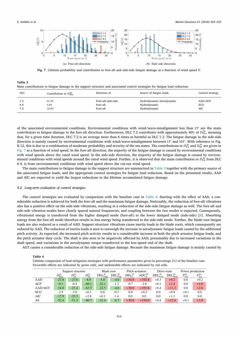
of the associated environmental conditions. Environmental conditions with wind/wave-misalignment less than ∘15 are the maincontributors to fatigue damage in the fore-aft direction. Furthermore, DLC 7.2 contributes with approximately 40% of DFA
20 , meaningthat, for a given time duration, DLC 7.2 is on average more than 6 times as harmful as DLC 1.2. The fatigue damage in the side-sidedirection is mainly caused by environmental conditions with wind/wave-misalignment between ∘15 and ∘105 . With reference to Fig.B.12, this is due to a combination of moderate probability and severity of the sea states. The contributions to DFA
20 and DSS20 are given in
Fig. 7 as a function of wind speed. In the fore-aft direction, the majority of the fatigue damage is caused by environmental conditionswith wind speeds above the rated wind speed. In the side-side direction, the majority of the fatigue damage is caused by environ-mental conditions with wind speeds around the rated wind speed. Further, it is observed that the main contribution to DFA
20 from DLC6.4, is from environmental conditions with wind speed above the cut-out wind speed.
The main contributions to fatigue damage in the support structure are summarized in Table 3 together with the primary source ofthe associated fatigue loads, and the appropriate control strategies for fatigue load reduction. Based on the presented results, AADand AIC are expected to yield the largest reductions in the lifetime accumulated fatigue damage.
4.2. Long-term evaluation of control strategies
The control strategies are evaluated by comparison with the baseline case in Table 4. Starting with the effect of AAD, a con-siderable reduction is achieved for both the fore-aft and the maximum fatigue damage. Noticeably, the reduction of fore-aft vibrationsalso has a positive effect on the side-side vibrations, resulting in a reduction of the side-side fatigue damage as well. The fore-aft andside-side vibration modes have closely spaced natural frequencies, and coupling between the two modes is expected. Consequently,vibrational energy is transferred from the higher damped mode (fore-aft) to the lower damped mode (side-side) [8]. Absorbingenergy from the fore-aft mode therefore results in less energy being transferred to the side-side mode. Further, the blade root fatigueloads are also reduced as a result of AAD. Support structure vibrations cause inertia loads in the blade roots, which consequently arereduced by AAD. The reduction of inertia loads is seen to outweigh the increase in aerodynamic fatigue loads caused by the additionalpitch activity. As expected, the increased pitch activity results in a considerable increase in both the pitch actuator fatigue loads, andthe pitch actuator duty cycle. The shaft is also seen to be negatively affected by AAD, presumably due to increased variations in theshaft speed, and variations in the aerodynamic torque transferred to the low-speed end of the shaft.
AGT causes a considerable reduction of the side-side fatigue damage. Because the maximum fatigue damage is mainly caused by
Fig. 7. Lifetime probability and contribution to fore-aft and side-side fatigue damage as a function of wind speed V.
Table 3Main contributions to fatigue damage in the support structure and associated control strategies for fatigue load reduction.
DLC Contribution to DMax20 Direction of Source of fatigue loads Control strategy
1.2 61.5% Fore-aft/side-side Hydrodynamic/Aerodynamic AAD/AGT6.4 5.6% Fore-aft Hydrodynamic SCO7.2 32.9% Fore-aft Hydrodynamic AIC
Table 4Lifetime comparison of load mitigation strategies with performance parameters given in percentage [%] of the baseline case.Favorable effects are indicated by green cells, and undesirable effects are indicated by red cells.
E. Smilden et al. Marine Structures 61 (2018) 503–523
514
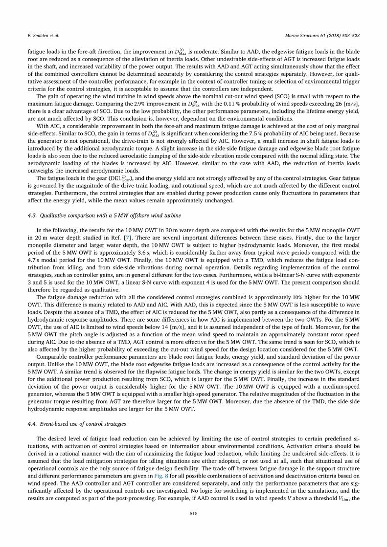
fatigue loads in the fore-aft direction, the improvement in DMax20 is moderate. Similar to AAD, the edgewise fatigue loads in the blade
root are reduced as a consequence of the alleviation of inertia loads. Other undesirable side-effects of AGT is increased fatigue loadsin the shaft, and increased variability of the power output. The results with AAD and AGT acting simultaneously show that the effectof the combined controllers cannot be determined accurately by considering the control strategies separately. However, for quali-tative assessment of the controller performance, for example in the context of controller tuning or selection of environmental triggercriteria for the control strategies, it is acceptable to assume that the controllers are independent.
The gain of operating the wind turbine in wind speeds above the nominal cut-out wind speed (SCO) is small with respect to themaximum fatigue damage. Comparing the 2.9% improvement in DMax
20 with the 0.11 % probability of wind speeds exceeding 26 [m/s],there is a clear advantage of SCO. Due to the low probability, the other performance parameters, including the lifetime energy yield,are not much affected by SCO. This conclusion is, however, dependent on the environmental conditions.
With AIC, a considerable improvement in both the fore-aft and maximum fatigue damage is achieved at the cost of only marginalside-effects. Similar to SCO, the gain in terms of DMax
20 is significant when considering the 7.5 % probability of AIC being used. Becausethe generator is not operational, the drive-train is not strongly affected by AIC. However, a small increase in shaft fatigue loads isintroduced by the additional aerodynamic torque. A slight increase in the side-side fatigue damage and edgewise blade root fatigueloads is also seen due to the reduced aeroelastic damping of the side-side vibration mode compared with the normal idling state. Theaerodynamic loading of the blades is increased by AIC. However, similar to the case with AAD, the reduction of inertia loadsoutweighs the increased aerodynamic loads.
The fatigue loads in the gear (DELGear20 ), and the energy yield are not strongly affected by any of the control strategies. Gear fatigue
is governed by the magnitude of the drive-train loading, and rotational speed, which are not much affected by the different controlstrategies. Furthermore, the control strategies that are enabled during power production cause only fluctuations in parameters thataffect the energy yield, while the mean values remain approximately unchanged.
4.3. Qualitative comparison with a 5MW offshore wind turbine
In the following, the results for the 10MW OWT in 30m water depth are compared with the results for the 5MW monopile OWTin 20m water depth studied in Ref. [7]. There are several important differences between these cases. Firstly, due to the largermonopile diameter and larger water depth, the 10MW OWT is subject to higher hydrodynamic loads. Moreover, the first modalperiod of the 5MW OWT is approximately 3.6 s, which is considerably farther away from typical wave periods compared with the4.7 s modal period for the 10MW OWT. Finally, the 10MW OWT is equipped with a TMD, which reduces the fatigue load con-tribution from idling, and from side-side vibrations during normal operation. Details regarding implementation of the controlstrategies, such as controller gains, are in general different for the two cases. Furthermore, while a bi-linear S-N curve with exponents3 and 5 is used for the 10MW OWT, a linear S-N curve with exponent 4 is used for the 5MW OWT. The present comparison shouldtherefore be regarded as qualitative.
The fatigue damage reduction with all the considered control strategies combined is approximately 10% higher for the 10MWOWT. This difference is mainly related to AAD and AIC. With AAD, this is expected since the 5MW OWT is less susceptible to waveloads. Despite the absence of a TMD, the effect of AIC is reduced for the 5MW OWT, also partly as a consequence of the difference inhydrodynamic response amplitudes. There are some differences in how AIC is implemented between the two OWTs. For the 5MWOWT, the use of AIC is limited to wind speeds below 14 [m/s], and it is assumed independent of the type of fault. Moreover, for the5MW OWT the pitch angle is adjusted as a function of the mean wind speed to maintain an approximately constant rotor speedduring AIC. Due to the absence of a TMD, AGT control is more effective for the 5MW OWT. The same trend is seen for SCO, which isalso affected by the higher probability of exceeding the cut-out wind speed for the design location considered for the 5MW OWT.
Comparable controller performance parameters are blade root fatigue loads, energy yield, and standard deviation of the poweroutput. Unlike the 10MW OWT, the blade root edgewise fatigue loads are increased as a consequence of the control activity for the5MW OWT. A similar trend is observed for the flapwise fatigue loads. The change in energy yield is similar for the two OWTs, exceptfor the additional power production resulting from SCO, which is larger for the 5MW OWT. Finally, the increase in the standarddeviation of the power output is considerably higher for the 5MW OWT. The 10MW OWT is equipped with a medium-speedgenerator, whereas the 5MW OWT is equipped with a smaller high-speed generator. The relative magnitudes of the fluctuation in thegenerator torque resulting from AGT are therefore larger for the 5MW OWT. Moreover, due the absence of the TMD, the side-sidehydrodynamic response amplitudes are larger for the 5MW OWT.
4.4. Event-based use of control strategies
The desired level of fatigue load reduction can be achieved by limiting the use of control strategies to certain predefined si-tuations, with activation of control strategies based on information about environmental conditions. Activation criteria should bederived in a rational manner with the aim of maximizing the fatigue load reduction, while limiting the undesired side-effects. It isassumed that the load mitigation strategies for idling situations are either adopted, or not used at all, such that situational use ofoperational controls are the only source of fatigue design flexibility. The trade-off between fatigue damage in the support structureand different performance parameters are given in Fig. 8 for all possible combinations of activation and deactivation criteria based onwind speed. The AAD controller and AGT controller are considered separately, and only the performance parameters that are sig-nificantly affected by the operational controls are investigated. No logic for switching is implemented in the simulations, and theresults are computed as part of the post-processing. For example, if AAD control is used in wind speeds V above a threshold VLim, the
E. Smilden et al. Marine Structures 61 (2018) 503–523
515
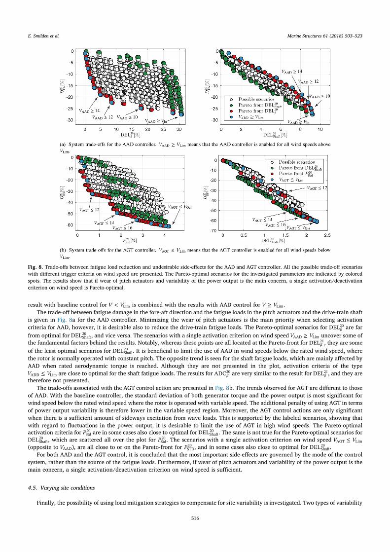
result with baseline control for <V VLim is combined with the results with AAD control for ≥V VLim.The trade-off between fatigue damage in the fore-aft direction and the fatigue loads in the pitch actuators and the drive-train shaft
is given in Fig. 8a for the AAD controller. Minimizing the wear of pitch actuators is the main priority when selecting activationcriteria for AAD, however, it is desirable also to reduce the drive-train fatigue loads. The Pareto-optimal scenarios for DELβ
20 are farfrom optimal for DELShaft
20 , and vice versa. The scenarios with a single activation criterion on wind speed ≥V VAAD Lim uncover some ofthe fundamental factors behind the results. Notably, whereas these points are all located at the Pareto-front for DELβ
20, they are someof the least optimal scenarios for DELShaft
20 . It is beneficial to limit the use of AAD in wind speeds below the rated wind speed, wherethe rotor is normally operated with constant pitch. The opposite trend is seen for the shaft fatigue loads, which are mainly affected byAAD when rated aerodynamic torque is reached. Although they are not presented in the plot, activation criteria of the type
≤V VADD Lim are close to optimal for the shaft fatigue loads. The results for ADCβ20 are very similar to the result for DELβ
20, and they aretherefore not presented.
The trade-offs associated with the AGT control action are presented in Fig. 8b. The trends observed for AGT are different to thoseof AAD. With the baseline controller, the standard deviation of both generator torque and the power output is most significant forwind speed below the rated wind speed where the rotor is operated with variable speed. The additional penalty of using AGT in termsof power output variability is therefore lower in the variable speed region. Moreover, the AGT control actions are only significantwhen there is a sufficient amount of sideways excitation from wave loads. This is supported by the labeled scenarios, showing thatwith regard to fluctuations in the power output, it is desirable to limit the use of AGT in high wind speeds. The Pareto-optimalactivation criteria for PStd
20 are in some cases also close to optimal for DELShaft20 . The same is not true for the Pareto-optimal scenarios for
DELShaft20 , which are scattered all over the plot for PStd
20 . The scenarios with a single activation criterion on wind speed ≤V VAGT Lim(opposite to VAAD), are all close to or on the Pareto-front for PSTD
20 , and in some cases also close to optimal for DELShaft20 .
For both AAD and the AGT control, it is concluded that the most important side-effects are governed by the mode of the controlsystem, rather than the source of the fatigue loads. Furthermore, if wear of pitch actuators and variability of the power output is themain concern, a single activation/deactivation criterion on wind speed is sufficient.
4.5. Varying site conditions
Finally, the possibility of using load mitigation strategies to compensate for site variability is investigated. Two types of variability
Fig. 8. Trade-offs between fatigue load reduction and undesirable side-effects for the AAD and AGT controller. All the possible trade-off scenarioswith different trigger criteria on wind speed are presented. The Pareto-optimal scenarios for the investigated parameters are indicated by coloredspots. The results show that if wear of pitch actuators and variability of the power output is the main concern, a single activation/deactivationcriterion on wind speed is Pareto-optimal.
E. Smilden et al. Marine Structures 61 (2018) 503–523
516

in site conditions are investigated; these are variability in water depth, and variability in soil conditions affecting the soil stiffness.Only site-specific variations which affect the modal properties of the OWT are considered. Site-specific variations in environmentalconditions such as wake effects, turbulence intensity, and sea states, are not considered. The only change applied to the wind turbineunder the varying site conditions, is tuning of the TMD to the modified first natural frequency of the support structure. When thevariation in water depth is considered, the monopile length is kept unchanged, and the water depth is scaled with a factor ηDepth. Themonopile penetration depth is adjusted to compensate for the change in water depth, meaning that if, for example, the water depth isincreased with 3m, the monopile penetration depth is reduced with 3m. The monopile penetration depth is primarily determinedbased on ULS considerations. The aim of the present analysis is to analyse the effect of variations in site conditions for a givenfoundation design. It is assumed that the change in water depth is within a range which does not require modification of the monopilepenetration depth. When variation in soil conditions is considered, the soil profile is kept unchanged, and the soil stiffness is scaledwith a factor ηSoil. The modal damping ratios are affected by changes in the modal characteristics resulting from the variations in siteconditions. The damping properties of the support structure are not modified to compensate for the variation in damping ratios.
The 20-year maximum fatigue damage over the circumference of the foundation with the baseline OWT controller is presented inFig. 9 as a function of ηSoil and ηDepth. The results are normalized with the baseline case ( = =η η 1.0Soil Depth ). Furthermore, thecorresponding variation in the first modal frequency, and the damping ratio is given in Fig. 10. Because the first modal frequencies inthe fore-aft and side-side direction are in close proximity, only the fore-aft frequency is presented. Variation in the soil conditionsaffects the mode shapes and natural frequencies of the support structure. Increased stiffness and damping leads to reduced vibrationamplitudes with less fatigue damage as a result, and vice versa. Moreover, the natural frequency is shifted closer to, or further away,from typical wave frequencies, altering the dynamic response to wave loads. Due to the large difference in damping between op-eration and idling, the changes in modal characteristics affect DLC 7.2 more than DLC 1.2. For this reason, the relative contribution tothe lifetime fatigue damage from DLC 7.2 increase as the stiffness- and damping-contribution from the soil is reduced. The results forvariation in water depth are similar to the results for soil variations, however, the monopile fatigue damage is seen to be even moresensitive to variations in the water depth. When the monopile penetration depth is changed, the modal characteristics are altered,affecting the natural frequencies and response amplitudes. In addition, the magnitude of the hydrodynamic loads depends on thewater depth, which adds to the sensitivity of fatigue loads to variations in the water depth.
Four different scenarios of variation in site conditions around the baseline design case are investigated in the context of controlstrategies for fatigue load reduction. Each scenario consists of two sub-cases, denoted as the reference case and the controlled case.The reference case is the site condition with the least amount of monopile fatigue damage out of the two sub-cases, and the controlledcase is the site condition for which the control strategies for fatigue load reduction is applied. The operational controls considered areAAD and AGT, and the use of these control strategies is restricted to the boundaries on the wind speed given in Table 5. Theseboundaries are chosen based on the previously presented results, assuming that the side-effects of primary interest are pitch actuatorwear, and the standard deviation of power output. Furthermore, the idling controllers AIC and SCO are applied for both the referencecases and the controlled cases to reduce the impact of DLC 6.4 and DLC 7.2.
First, the effect of variations in site conditions on the performance of the control strategies is investigated. Identical to the analysisperformed in Sec. 4.2, the lifetime effect of permanently enabled control strategies is presented for =η 0.8soil , and =η 1.05soil inAppendix A. In both cases the global stiffness and damping are reduced compared with the baseline case, resulting in higher responseamplitudes, and increased effectiveness of AGT and AIC. The cost is a moderate increase in collateral effects, particularly for the AGTcontroller. The AAD control activity is only marginally affected by the changes in site conditions. However, the influence of AAD on
Fig. 9. Normalized maximum fatigue damage over the circumference of the foundation under varying site conditions. Results are presented for thecritical cross-section 6m below the mudline.
Fig. 10. Variations in the fore-aft modal frequency fFA and the fore-aft damping ratio ζFA under varying site conditions.
E. Smilden et al. Marine Structures 61 (2018) 503–523
517
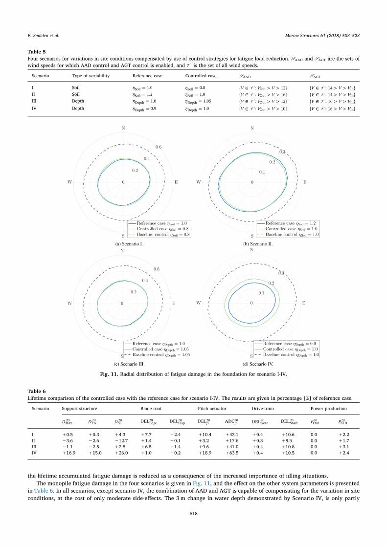
the lifetime accumulated fatigue damage is reduced as a consequence of the increased importance of idling situations.The monopile fatigue damage in the four scenarios is given in Fig. 11, and the effect on the other system parameters is presented
in Table 6. In all scenarios, except scenario IV, the combination of AAD and AGT is capable of compensating for the variation in siteconditions, at the cost of only moderate side-effects. The 3m change in water depth demonstrated by Scenario IV, is only partly
Table 5Four scenarios for variations in site conditions compensated by use of control strategies for fatigue load reduction. AADS and AGTS are the sets ofwind speeds for which AAD control and AGT control is enabled, andV is the set of all wind speeds.
Scenario Type of variability Reference case Controlled case AADS AGTS
I Soil =η 1.0Soil =η 0.8Soil ∈ > >V V V{ : 12}OutV ∈ > >V V V{ : 14 }InV
II Soil =η 1.2Soil =η 1.0Soil ∈ > >V V V{ : 16}OutV ∈ > >V V V{ : 14 }InV
III Depth =η 1.0Depth =η 1.05Depth ∈ > >V V V{ : 12}OutV ∈ > >V V V{ : 16 }InV
IV Depth =η 0.9Depth =η 1.0Depth ∈ > >V V V{ : 10}OutV ∈ > >V V V{ : 16 }InV
Fig. 11. Radial distribution of fatigue damage in the foundation for scenario I-IV.
Table 6Lifetime comparison of the controlled case with the reference case for scenario I-IV. The results are given in percentage [%] of reference case.
Scenario Support structure Blade root Pitch actuator Drive-train Power production
DMax20 DFA
20 DSS20 DELEdge
20 DELFlap20 DELβ
20 ADCβ20 DELGear
20 DELShaft20 POut
20 PSTD20
I +0.5 +0.3 +4.3 +7.7 +2.4 +10.4 +43.1 +0.4 +10.6 0.0 +2.2II −3.6 −2.6 −12.7 +1.4 −0.1 +3.2 +17.6 +0.3 +8.5 0.0 +1.7III −1.1 −2.5 +2.8 +6.5 −1.4 +9.6 +41.0 +0.4 +10.8 0.0 +3.1IV +16.9 +15.0 +26.0 +1.0 −0.2 +18.9 +63.5 +0.4 +10.5 0.0 +2.4
E. Smilden et al. Marine Structures 61 (2018) 503–523
518
counteracted by the operational controls, and the pitch actuators are severely affected by the control action compared with the otherscenarios. The ability of the operational controls to compensate for variations in the site conditions depends on the global stiffnessand damping. Comparing, for example, scenario I with scenario II, the difference in support structure fatigue damage resulting fromthe change in soil stiffness is lower for scenario II. Consequently, the adverse side-effects to the pitch actuators are less severe forscenario II. The same trend is observed for variations in the water depth.
5. Conclusions
The present work analysed the applicability of control system design to compensate for differing fatigue loads in the supportstructure due to varying site conditions. The design case was a 10 MW offshore wind turbine in 30 m water depth at the DoggerBank in the North Sea. Long-term variations in environmental conditions given by 60-years of hindcast data for the designlocation were combined with short-term aero-hydro-servo elastic simulations in the 20-year assessment of the fatigue strengthfor the support structure. Control strategies applicable for both normal operation and idling situations were considered. Theoperational control strategies included active aerodynamic damping control for reduction of fatigue loads in the fore-aft di-rection, and active generator torque control for reduction of fatigue loads in the side-side direction. The idling control stra-tegies included active idling control and soft cut-out control, both primarily for reduction of fatigue loads in the fore-aftdirection.
For the baseline design case, the fatigue damage was nonuniformly distributed around the circumference of the support structure,with southwest/northeast being the most critical orientations. This corresponded with the primary direction of wind and wind-sea,which for the design location is southwest. Approximately 20% of the total fatigue damage was caused by wave loads acting in theside-side direction, and despite only 10% unavailability, this design situation contributed with approximately 35% of the total fatiguedamage. Further, the performance of the control strategies in terms of fatigue load reduction, and effect on other wind turbinecomponents, was analysed. Results showed that a total fatigue load reduction of approximately 50% was possible, at the cost ofincreased wear of pitch actuators, increased fatigue loads in the drive-train shaft, and increased fluctuations in the power output.Other system parameters were only moderately affected. Undesirable side-effects may be significantly reduced by limiting the use ofthe operational control strategies to some predefined situations. Particularly, the wear of pitch actuators due to active aerodynamicdamping, was reduced by approximately 50% by restricting the use of this control strategy to wind speeds above the rated wind speed.It was also shown that the fluctuations in power output could be reduced by limiting the use of active generator torque control in highwind speeds.
Two types of variability in the site conditions were investigated: variations in soil conditions affecting the soil stiffness, andvariations in the water depth. The fatigue loads in the support structure were more sensitive to variations in the water depththan to variations in the soil conditions. Furthermore, due to the large difference in system damping between operation andidling, the relative contribution to fatigue damage from idling conditions increased with decreasing soil stiffness. Further, theoperational control strategies were used to compensate for the changes in fatigue loads arising from the variations in siteconditions. With only moderate cost to other system components, the control system was able to compensate for a 20% variationin soil stiffness. Similar results were achieved with a 5% (1.5 m) increase in water depth. The control system was not fullycapable of compensating for a 10% increase in water depth from 27 m to 30 m, and the undesirable side-effects were more severecompared with the other scenarios.
The results indicated that the wind turbine's control system is useful for compensating for variations in the soil conditions. Theresults with respect to water depth were less promising. There is a clear advantage of the presented methodology in terms of reducingthe design conservatism associated with foundation clustering including also variations in water depth. However, limiting the scopeto soil variability, and including also uncertainty in soil parameters, is likely a more suitable application. The adverse side-effectsassociated with the presented methodology were not insignificant. Control strategies and methodology to further improve the trade-off between support structure fatigue damage and adverse side-effects should be developed. Active aerodynamic damping had themost severe side-effects. For large OWTs in moderate water depth, such as the present design case, severe sea states represent aconsiderable contribution to the lifetime accumulated fatigue damage. In severe sea states, the wave induced motion is dominated bythe quasi-static response, which is governed by the global stiffness. Active pitch control to increase both the damping and stiffness ofthe fore-aft vibration modes is therefore a strategy which should be explored. Finally, considering the large potential for fatigue loadreduction with active idling control, the literature on this control strategy is sparse. Further research on active idling control isrecommended.
Acknowledgments
This work has been carried out at the Center for Autonomous Marine Operations and Systems (NTNU AMOS). TheNorwegian Research Council is acknowledged as the main sponsor of NTNU AMOS. This work was supported by the ResearchCouncil of Norway through the Centres of Excellence funding scheme, Project number 223254 - NTNU AMOS. Theauthors would also like to thank Dr. Amir R. Nejad for his invaluable assistance on aspects regarding drive-train fatiguecalculations.
E. Smilden et al. Marine Structures 61 (2018) 503–523
519

Appendix A. Supplementary data
Supplementary data related to this article can be found at http://dx.doi.org/10.1016/j.marstruc.2018.03.002.
Appendix A. Control strategy comparison under varying site conditions
Table A.7Lifetime comparison of load mitigation strategies with performance parameters given in percentage [%] of the baselinecontrol case with =η 0.8Soil .
Table A.8:Lifetime comparison of load mitigation strategies with performance parameters given in percentage [%] of the baselinecontrol case with =η 1.05Depth .
E. Smilden et al. Marine Structures 61 (2018) 503–523
520

Appendix B. Environmental load cases
Figure B.12. Environmental load cases (ELC) for each group of wind/wave misalignment ψ.
E. Smilden et al. Marine Structures 61 (2018) 503–523
521

References
[1] Ho A, Mbistrova A, Corbetta G, Pineda I, Ruby K. The european offshore wind industry-key trends and statistics Brussels: European Wind Energy Association;2016. Report.
[2] P. Gardner, A. Garrad, P. Jamieson, H. Snodin, A. Tindal, Wind Energy–The Facts, Technology, Part I.[3] Shrestha B, Kühn M. Tailoring the employment of offshore wind turbine support structure load mitigation controllers. Journal of physics: conference series, vol.
753. IOP Publishing; 2016. p. 052032.[4] Bachynski EE, Ormberg H. Hydrodynamic modeling of large-diameter bottom-fixed offshore wind turbines. ASME 2015 34th international conference on ocean,
offshore and arctic engineering. American Society of Mechanical Engineers; 2015. p. V009T09A051.[5] Fischer T, Vries W, Rainey P, Schmidt B, Argyriadis K, Kühn M. Offshore support structure optimization by means of integrated design and controls. Wind Energy
2012;15(1):99–117.[6] Smilden E, Bachynski EE, Sørensen AJ. Key contributors to lifetime accumulated fatigue damage in an offshore wind turbine support structure. ASME 2017 36th
International Conference on Ocean, Offshore and Arctic Engineering. American Society of Mechanical Engineers; 2017. p. V010T09A075.[7] Fischer TA. Mitigation of Aerodynamic and Hydrodynamic Induced Loads of Offshore Wind Turbines. Shaker: University of Stuttgart; 2012.[8] Damgaard M, Ibsen LB, Andersen LV, Andersen JK. Cross-wind modal properties of offshore wind turbines identified by full scale testing. J Wind Eng Ind Aerod
2013;116:94–108.[9] Devriendt C, Jordaens PJ, De Sitter G, Guillaume P. Damping estimation of an offshore wind turbine on a monopile foundation. IET Renew Power Gener
2013;7(4):401–12.[10] Shirzadeh R, Devriendt C, Bidakhvidi MA, Guillaume P. Experimental and computational damping estimation of an offshore wind turbine on a monopile
foundation. J Wind Eng Ind Aerod 2013;120:96–106.[11] E. Van der Hooft, P. Schaak, T. Van Engelen, Wind Turbine Control Algorithms, DOWEC project-DOWEC-F1W1-EH-03–094/0, Task-3 report.[12] Bossanyi E. Wind turbine control for load reduction. Wind Energy 2003;6(3):229–44.[13] Bossanyi E, Ramtharan G, Savini B. The importance of control in wind turbine design and loading. Control and Automation, 2009. MED’09. 17th Mediterranean
Conference on. IEEE; 2009. p. 1269–74.[14] B. Fischer, M. Shan, A survey on control methods for the mitigation of tower loads, Fraunhofer-Institute for Wind Energy and Energy Systems Technology, IWES
Project report 01/104256.[15] Shan M, Jacobsen J, Adelt S. Field testing and practical aspects of load reducing pitch control systems for a 5 mw offshore wind turbine. Proc. EWEA 2013:101–5.[16] Trumars JM, Jonsson JO, Bergdahl L. The effect of wind and wave misalignment on the response of a wind turbine at Bockstigen. 25th international conference
on offshore mechanics and arctic engineering. American Society of Mechanical Engineers; 2006. p. 635–41.[17] Horn J-TH, Krokstad J, Amdahl J. Joint probability distribution of environmental conditions for design of offshore wind turbines. ASME 2017 36th international
conference on ocean, offshore and arctic engineering. American Society of Mechanical Engineers; 2017. p. V010T09A068.[18] Fischer T, Rainey P, Bossanyi E, Kühn M. Study on control concepts suitable for mitigation of loads from misaligned wind and waves on offshore wind turbines
supported on monopiles. Wind Eng 2011;35(5):561–73.[19] Zhang Z, Nielsen SR, Blaabjerg F, Zhou D. Dynamics and control of lateral tower vibrations in offshore wind turbines by means of active generator torque.
Energies 2014;7(11):7746–72.[20] Ziegler L, Voormeeren S, Schafhirt S, Muskulus M. Sensitivity of wave fatigue loads on offshore wind turbines under varying site conditions. Energy Procedia
2015;80:193–200.[21] Damgaard M, Andersen LV, Ibsen LB. Dynamic response sensitivity of an offshore wind turbine for varying subsoil conditions. Ocean Eng 2015;101:227–34.[22] Schafhirt S, Page A, Eiksund GR, Muskulus M. Influence of soil parameters on the fatigue lifetime of offshore wind turbines with monopile support structure.
Energy Procedia 2016;94:347–56.[23] Ziegler L, Voormeeren S, Schafhirt S, Muskulus M. Design clustering of offshore wind turbines using probabilistic fatigue load estimation. Renew Energy
2016;91:425–33.[24] Carswell W, Arwade SR, DeGroot DJ, Lackner MA. Soil–structure reliability of offshore wind turbine monopile foundations. Wind Energy 2015;18(3):483–98.[25] Damgaard M, Andersen LV, Ibsen LB, Toft HS, Sørensen JD. A probabilistic analysis of the dynamic response of monopile foundations: soil variability and its
consequences. Probabilist Eng Mech 2015;41:46–59.[26] P. Tavner, Offshore wind turbines: reliability, availability and maintenance, The Institution of Engineering and Technology, London, UK.[27] Wilkinson M, Hendriks B, Spinato F, Harman K, Gomez E, Bulacio H, Roca J, Tavner P, Feng Y, Long H. Methodology and results of the reliawind reliability field
study. European wind energy conference and exhibition 2010, EWEC 2010, vol. 3. 2010. p. 1984–2004. Sheffield.[28] Bianchi FD, De Battista H, Mantz RJ. Wind turbine control systems: principles, modelling and gain scheduling design. Springer Science & Business Media; 2006.[29] Perrone F, Kühn M. Offshore wind turbine tower fore-aft fatigue load reduction by coupling control and vibrational analysis. J. Ocean and Wind Energy
2015;2(3):168–75.[30] Perrone F. Offshore wind turbine tower fore-aft control: trade-off fatigue load reduction and pitch activity. European Control Conference (ECC), 2015. IEEE;
2015. p. 2444–8.[31] Shrestha B, Kühn M. Adaptation of controller concepts for support structure load mitigation of offshore wind turbines. Energy Procedia 2016;94:241–8.[32] C. Bak, F. Zahle, R. Bitsche, T. Kim, A. Yde, L. Henriksen, A. Natarajan, M. Hansen, Description of the DTU 10 MW reference wind turbine, DTU Wind Energy
Report-I-0092.[33] M. Reistad, Ø.Breivik, H.Haakenstad, O. J.Aarnes, B. R.Furevik, J.-R.Bidlot, A high-resolution hindcast of wind and waves for the North sea, the Norwegian sea,
and the Barents Sea, J Geophys Res: Oceans 116(C5).[34] Brodtkorb PA, Johannesson P, Lindgren G, Rychlik I, Rydén J, Sjö E, et al. Wafo-a matlab toolbox for analysis of random waves and loads. The tenth international
offshore and polar engineering conference. International Society of Offshore and Polar Engineers; 2000.[35] Markou H, Larsen TJ. Control strategies for operation of pitch regulated turbines above cut-out wind speeds. 2009 European Wind Energy Conference and
Exhibition. 2009.[36] Hansen MH, Henriksen LC. Basic DTU wind energy controller. Tech. rep., DTU Wind Energy; 2013.[37] W. Carswell, Soil-structure modeling and design considerations for offshore wind turbine monopile foundations.[38] Stewart GM, Lackner MA. The impact of passive tuned mass dampers and wind–wave misalignment on offshore wind turbine loads. Eng Struct 2014;73:54–61.[39] DNV GL, Loads and site conditions for wind turbines, DNVGL-ST-0437.[40] International Electrotechnical Commission (IEC). IEC 61400–61401: wind turbines part 1: design requirements. Tech. rep.; 2005.[41] Kühn MJ. Dynamics and design optimisation of offshore wind energy conversion systems. TU Delft: Delft University of Technology; 2001.[42] DNV GL, DNV-RP-C205, Environmental conditions and environmental loads.[43] B. J. Jonkman, Turbsim user's guide: version 1.50.[44] Carroll J, McDonald A, Dinwoodie I, McMillan D, Revie M, Lazakis I. Availability, operation and maintenance costs of offshore wind turbines with different drive
train configurations. Wind Energy 2017;20(2):361–78.[45] API RP. Recommended practice for geotechnical foundation design consideration. 2GEO. 2011.[46] Ormberg H, Bachynski EE, et al. Global analysis of floating wind turbines: code development, model sensitivity and benchmark study. The twenty-second
international offshore and polar engineering conference. International Society of Offshore and Polar Engineers; 2012.[47] Faltinsen O. Sea loads on ships and offshore structures vol. 1. Cambridge university press; 1993.[48] Matsuishi M, Endo T. Fatigue of metals subjected to varying stress. 68. Fukuoka, Japan: Japan Society of Mechanical Engineers; 1968. p. 37–40. 2.[49] DNV GL, Fatigue Design of Offshore Steel Structures, No. DNV-RP-C203.[50] DNV GL, OS-C101, Design of Offshore Steel Structures, General (LRFD Method).
E. Smilden et al. Marine Structures 61 (2018) 503–523
522

[51] Freebury G, Musial WD. Determining Equivalent Damage Loading for Full-Scale Wind Turbine Blade Fatigue Tests. CO: National Renewable Energy LaboratoryGolden; 2000.
[52] Burton T, Sharpe D, Jenkins N, Bossanyi E. Wind Energy Handbook. second ed. John Wiley & Sons; 2011.[53] Nejad AR, Gao Z, Moan T. On long-term fatigue damage and reliability analysis of gears under wind loads in offshore wind turbine drivetrains. Int J Fatig
2014;61:116–28.[54] B. Niederstucke, A. Anders, P. Dalhoff, R. Grzybowski, reportLoad Data Analysis for Wind Turbine Gearboxes, Final report of enhanced life analysis of wind
power systems.[55] Bottasso C, Campagnolo F, Croce A, Tibaldi C. Optimization-based study of bend–twist coupled rotor blades for passive and integrated passive/active load
alleviation. Wind Energy 2013;16(8):1149–66.[56] Standard, ISO, 6336–6. Calculation of Load Capacity of Spur and Helical Gears Part 6: Calculation of Service Life Under Variable Load. Geneva, Switzerland:
International Organization for Standardization; 2006.[57] Standard, ISO, 6336–3. Calculation of Load Capacity of Spur and Helical Gears Part 6: Calculation of Tooth Bending Stress. Geneva, Switzerland: International
Organization for Standardization; 2006.[58] Stol KA, Zhao W, Wright AD. Individual blade pitch control for the controls advanced research turbine. J Sol Energy Eng 2006;128(4):498–505.[59] Devriendt C, Jordaens P, Sitter G, Guillaume P. Damping estimation of an offshore wind turbine on a monopile foundation. IET Renew Power Gener
2013;7(4):401–12.[60] Hansen MH, Thomsen K, Fuglsang P, Knudsen T. Two methods for estimating aeroelastic damping of operational wind turbine modes from experiments. Wind
Energy 2006;9(1–2):179–91.
E. Smilden et al. Marine Structures 61 (2018) 503–523
523

Received: 2 March 2018 Revised: 3 July 2018 Accepted: 17 August 2018
DOI: 10.1002/we.2273
R E S E A R C H A R T I C L E
Wave disturbance rejection for monopile offshore windturbines
Emil Smilden Erin E. Bachynski Asgeir J. Sørensen Jørgen Amdahl
Centre for Autonomous Marine Operations
and Systems, Department of Marine
Technology, Norwegian University of Science
and Technology, Trondheim, Norway
Correspondence
Emil Smilden, Centre for Autonomous Marine
Operations and Systems, Department of
Marine Technology, Norwegian University of
Science and Technology, Trondheim, Norway.
Email: [email protected]
Funding information
The Norwegian Research council,
Grant/Award Number: 223254
Abstract
The dimensions of offshore wind turbine (OWT) support structures are governed by fatigue
considerations. For 6- to 10-MW OWTs, wave loads are often dominating in terms of
fatigue utilization. The present work proposes a control scheme to reduce the wave-induced
fatigue loads in OWT support structures. The control scheme applies collective pitch control
to increase both the damping and stiffness of the fore-aft vibration modes. With conventional
active tower damping, efficient wave disturbance rejection is restricted to a narrow frequency
range around the first fore-aft modal frequency. The proposed control scheme achieves efficient
wave disturbance rejection across a broader frequency range. Here, tower feedback control is
implemented via an auxiliary control loop. Based on a low-fidelity model, the effect of the tower
feedback loop on the stability margins of the basic controller is analysed. The results show
that, within certain boundaries, the stability margins are improved by the stiffness term in the
tower feedback loop. Consequently, the need to reduce the bandwidth of the basic controller
to accommodate tower feedback control is relaxed. Based on time-domain simulations carried
out in an aero-hydro-servo-elastic simulation tool, the lifetime effects of the proposed control
scheme are analysed. Compared with conventional active tower damping, a more favourable
trade-off between adverse side effects and the support structure's fatigue damage is achieved
with the proposed control scheme.
KEYWORDS
collective pitch control, fatigue load reduction, foundation design, offshore wind turbines, state
estimation
1 INTRODUCTION
With the commissioning of the first 8-MW wind turbine,1 the European offshore wind industry continues its advance towards larger wind
turbines. Most offshore wind farms are located in water depth less than 40 m, and monopiles are the preferred foundation type with a
market share close to 90%.1 Upscaling of the turbines poses a continuous challenge to the cost-efficiency of monopile foundations.2 Monopile
dimensions are mainly governed by fatigue considerations. With the introduction of even larger offshore wind turbines (OWTs), the first-order
wave loads become dominating in terms of fatigue utilization.3 Besides increased wave loads due to larger dimensions, the modal frequencies of
the OWTs are shifted closer to typical wave frequencies, thereby increasing the dynamic amplification of the wave-induced response.3,4
The wind turbine's control system affects the dynamic response of the OWT. Several control strategies that aim to reduce fatigue loads in the
support structure have been proposed.4-8 The conventional approach is collective pitch control to increase the aerodynamic damping of the first
fore-aft vibration mode.5,6 Supplementary damping is effective for reducing the response induced by wave loads with frequency close to the first
fore-aft modal frequency. This is usually the case for wind-generated waves in low and moderate wind conditions. For wind-generated waves in
high wind conditions and most occurrences of swell dominated sea, the wave frequencies are comparatively far below the fore-aft frequency.
Consequently, the wave response is dominated by the quasi-static response which is governed by the global stiffness. In order to effectively
Wind Energy. 2018;1–20. wileyonlinelibrary.com/journal/we © 2018 John Wiley & Sons, Ltd. 1
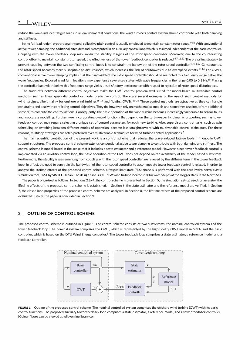
2 SMILDEN ET AL.
reduce the wave-induced fatigue loads in all environmental conditions, the wind turbine's control system should contribute with both damping
and stiffness.
In the full load region, proportional-integral collective pitch control is usually employed to maintain constant rotor speed.9,10 With conventional
active tower damping, the additional pitch demand is computed in an auxiliary control loop which is assumed independent of the basic controller.
Coupling with the tower feedback loop may impair the stability margins of the rotor speed controller. Moreover, due to the counteracting
control effort to maintain constant rotor speed, the effectiveness of the tower feedback controller is reduced.4,7,11,12 The prevailing strategy to
prevent coupling between the two conflicting control loops is to constrain the bandwidth of the rotor speed controller.4,7,11,12 Consequently,
the rotor speed becomes more susceptible to disturbances, which increases the risk of shutdowns due to overspeed events.13,14 For OWTs,
conventional active tower damping implies that the bandwidth of the rotor speed controller should be restricted to a frequency range below the
wave frequencies. Exposed wind farm locations may experience severe sea states with wave frequencies in the range 0.05 to 0.1 Hz.15 Placing
the controller bandwidth below this frequency range yields unsatisfactory performance with respect to rejection of rotor speed disturbances.
The trade-offs between different control objectives make the OWT control problem well suited for model-based multivariable control
methods, such as linear quadratic control or model predictive control. There are several examples of the use of such control methods for
wind turbines, albeit mainly for onshore wind turbines16-18 and floating OWTs.19-21 These control methods are attractive as they can handle
constraints and deal with conflicting control objectives. They do, however, rely on mathematical models and sometimes also input from additional
sensors, to compute the control actions. Consequently, the basic operation of the wind turbine becomes increasingly vulnerable to sensor faults
and inaccurate modelling. Furthermore, incorporating control functions that depend on the turbine-specific dynamic properties, such as tower
feedback control, may require selecting a unique set of control parameters for each new turbine. Also, supervisory control tasks, such as gain
scheduling or switching between different modes of operation, become less straightforward with multivariable control techniques. For these
reasons, multiloop strategies are often preferred over multivariable techniques for wind turbine control applications.7
The main scientific contribution of the present work is a control scheme that reduces the wave-induced fatigue loads in monopile OWT
support structures. The proposed control scheme extends conventional active tower damping to contribute with both damping and stiffness. The
control scheme is model-based in the sense that it includes a state estimator and a reference model. However, since tower feedback control is
implemented via an auxiliary control loop, the basic operation of the OWT does not depend on the availability of the model-based subsystem.
Furthermore, the stability issues emerging from coupling with the rotor speed controller are relieved by the stiffness term in the tower feedback
loop. In effect, the need to constrain the bandwidth of the rotor speed controller to accommodate tower feedback control is relaxed. In order to
analyse the lifetime effects of the proposed control scheme, a fatigue limit state (FLS) analysis is performed with the aero-hydro-servo-elastic
simulation tool SIMA by SINTEF Ocean. The design case is a 10-MW wind turbine located in 30 m water depth at the Dogger Bank in the North Sea.
The paper is organized as follows: In Sections 2 to 4, the control scheme is presented. In Section 5, the simulation set-up used for assessing the
lifetime effects of the proposed control scheme is established. In Section 6, the state estimator and the reference model are verified. In Section
7, the closed loop properties of the proposed control scheme are analysed. In Section 8, the lifetime effects of the proposed control scheme are
evaluated. Finally, the paper is concluded in Section 9.
2 OUTLINE OF CONTROL SCHEME
The proposed control scheme is outlined in Figure 1. The control scheme consists of two subsystems: the nominal controlled system and the
tower feedback loop. The nominal system comprises the OWT, which is represented by the high-fidelity OWT model in SIMA, and the basic
controller, which is based on the DTU Wind Energy controller.9 The tower feedback loop comprises a state estimator, a reference model, and a
feedback controller.
FIGURE 1 Outline of the proposed control scheme. The nominal controlled system comprises the offshore wind turbine (OWT) with its basiccontrol functions. The proposed auxiliary tower feedback loop comprises a state estimator, a reference model, and a tower feedback controller[Colour figure can be viewed at wileyonlinelibrary.com]

SMILDEN ET AL. 3
The wind turbine's basic control system operates in one of two modes with operational regions separated by the rated wind speed. In the
partial load region, the control objective is to maximize power production, and the wind turbine is operated with variable speed aiming to track
the optimal tip-speed ratio. In the full load region, the control objective is to confine the rotational speed and power production to their rated
values, and variable pitch is applied to control the aerodynamic torque. A third mode in which the control system operates with both variable
speed and variable pitch is often added in a wind speed range around the rated wind speed. This is usually referred to as peak shaving, and the
goal is to limit the aerodynamic thrust that peaks at the rated wind speed.9 The basic wind turbine control functions are implemented without
significant modifications. No peak shaving is performed with the default settings.
Tower feedback control is implemented via an auxiliary control loop, which receives measurements directly from the OWT. The main control
objective of the proposed tower feedback loop is to reduce the wave-induced fatigue loads in the support structure. Proportional-derivative
collective pitch control is employed to provide the support structure with additional damping and stiffness in the fore-aft direction. Proportional
action on the tower displacement with a zero reference input would introduce a steady-state rotor speed error. Therefore, a reference model is
employed to produce a nonzero reference trajectory representing the wind-induced tower displacement. In effect, the tower feedback loop only
provides stiffness against wave-induced tower displacements in a frequency range above the frequencies of significant turbulent wind variations.
Typically, information about the tower displacements is not available with standard wind turbine measurements. In addition, the reference model
requires information about the rotor wide effective wind speed, which cannot be measured directly. A state estimator is therefore needed in the
tower feedback loop. A discrete-time extended Kalman filter is formulated to calculate the required state estimates.
The state estimator and the reference model are based on a low-fidelity OWT model. The key components of the low-fidelity model are the
effective wind speed model proposed by Knudsen et al,22 the single-state dynamic inflow model proposed by Henriksen et al,23 and a wave
disturbance model, which is established in the present work.
3 LOW-FIDELITY OWT MODEL
The low-fidelity OWT model applied in the tower feedback loop is established in the following. The model comprises mathematical descriptions
of the support structure, drive-train, aerodynamic loads, hydrodynamic loads, and environmental conditions.
3.1 Support structure model
Modal analysis is employed to describe the fore-aft response of the support structure. The fore-aft response of monopile OWTs is dominated
by the first vibration mode,24 and higher-order modes are omitted from the model. Aerodynamic thrust and wave loads are assumed to be the
only external loads acting on the support structure, as shown in Figure 2. By introducing the generalized coordinate x = q(z)x, the second-order
differential equation describing the response of the support structure is given by
(m + q2(h)M) x + c x + kx = q(h)FA⏟⏟⏟
FA
+ ∫𝜁
−dq(z)FH(z) cos(𝜓)dz
⏟⏞⏞⏞⏞⏞⏞⏞⏞⏞⏞⏞⏞⏞⏞⏟⏞⏞⏞⏞⏞⏞⏞⏞⏞⏞⏞⏞⏞⏞⏟FH
, (1)
where x, x, x are the generalized fore-aft displacement, velocity, and acceleration, respectively, and M is the mass of the rotor-nacelle assembly.
The mode shape q(z), generalized mass m, generalized stiffness k, and the generalized damping c are extracted from the high-fidelity model
based on eigenvalue analysis and decay tests, respectively. The generalized hydrodynamic force FH is given by the fore-aft component of the
hydrodynamic load distribution FH(z) cos𝜓 multiplied with the mode shape and integrated from the seabed (z = −d) to the instantaneous
free surface (z = 𝜁 ). The hydrodynamic load distribution is decomposed according to the wind/wave misalignment angle 𝜓 . The generalized
aerodynamic thrust FA is given by the aerodynamic thrust FA multiplied with the mode shape at the tower top q(h) = 1.
The proposed model assumes that the modal properties of the support structure are known. Whereas the distribution of mass is usually
well known, the stiffness and damping properties are often uncertain. In particular, the site-specific soil properties are associated with large
uncertainties, and they may change throughout the lifetime of the OWT.25-27 Therefore, the true modal characteristics of monopile OWTs
are generally not known until they are installed.28 Although several methods to determine the modal characteristics of installed OWTs can be
found,28-30 the effect of erroneous modal properties needs to be addressed. The effect of modelling errors on state estimation is examined in
Section 6.
3.2 Drive-train model
The drive-train comprises the rotor and generator connected by a low-speed shaft, the generator, and a high-speed shaft. In the present work, the
shaft torsional flexibility is neglected, and the drive-train is modelled as a multibody system with two rigid bodies connected by a stiff member.
The angular velocity 𝜔 at the low-speed end of the shaft is governed by the first-order differential equation given by
�� = 1I(QA − NGQG), I = IR + N2
GIG, (2)

4 SMILDEN ET AL.
FIGURE 2 Definition of offshore wind turbine (OWT) coordinates and excitation forces
where QA is the aerodynamic torque applied at the low-speed end of the shaft and QG is the generator torque applied at the high-speed end of
the shaft.16 Furthermore, the rotor inertia IR and generator inertia IG are combined to form an equivalent inertia I, where NG is the gear ratio.
3.3 Aerodynamic model
Reduced-order models used for wind speed estimation are usually based on the assumption of a quasi-steady wake, meaning that the wake is
assumed at equilibrium. In reality, the wake does not settle at steady-state conditions immediately after a change in the operating conditions.
The timescale of the temporal wake dynamics is on the order of the rotor radius divided by the free stream velocity.31 In most environmental
conditions, the pitch control actions act within the same timescale as the temporal wake dynamics. Moreover, if the dynamic wake effect is
not accounted for, the aerodynamic damping is not represented correctly. Several control-oriented models that aim to capture the dynamic
wake effect, often referred to as dynamic inflow models, have been developed.23,32,33 Here, the single-state dynamic inflow model proposed by
Henriksen et al23 is used. This model is a simplification of the dynamic inflow model proposed by Øye,34 which is typically applied in aero-elastic
software codes.35
For a wind turbine with NB blades, the rotor wide aerodynamic thrust FA(·) and torque QA(·) are given by
FA(v, 𝛽, 𝜔, vn) = NB ∫R
0Fn (v, 𝛽, 𝜔, r, vn(r)) dr, (3)
QA(v, 𝛽, 𝜔, vn) = NB ∫R
0rFt (v, 𝛽, 𝜔, r, vn(r)) dr, (4)
where Fn(·) and Ft(·) are the local aerodynamic forces normal and tangential to the rotor plane at radius r, respectively. The local aerodynamic
forces depend on the pitch angle 𝛽 , rotor speed 𝜔, relative wind speed v = v0 − x, where v0 is the mean wind speed and vn(r) is the local induced
velocity normal to the rotor plane. The tangential induced velocities are assumed to be quasi-steady, and the distribution of vn(r) along the blades
is assumed to follow the quasi-steady distribution. This allows for the local induced velocities to be expressed by a single dynamic inflow state vn
following the relationship given by
vn(r) =aqs
n (𝜆, 𝛽, r)aqs
n (𝜆, 𝛽)vn, aqs
n (𝜆, 𝛽) = 1R ∫
R
0aqs
n (𝜆, 𝛽, r)dr > 0, (5)
where aqsn (𝜆, 𝛽, r) is the local quasi-steady axial induction factor and aqs
n (𝜆, 𝛽) is the average quasi-steady axial induction factor. The dynamic inflow
state is governed by the following non-linear first-order differential equation:
vn = 1𝜏(v, vn)
(aqs
n (𝜆, 𝛽)v − vn
), 𝜏(v, vn) =
12
1.1Rv − 1.3vn
. (6)
The timescale variable 𝜏(v, vn) is based on the model suggested by Øye34 and modified in accordance with Henriksen et al.23 Blade element
momentum (BEM) theory is employed to compute the quasi-steady induction factors following the procedure described by Hansen.35 In the
BEM calculations, the blades are assumed to be rigid, and the rotor cone and tilt angles are neglected.

SMILDEN ET AL. 5
3.4 Hydrodynamic load model
Hydrodynamic loads on large diameter monopile foundations, such as the present design case, are dominated by inertia loads.36 Moreover, the
monopile diameter is sufficiently large compared with typical wave lengths, so diffraction effects should be accounted for. The hydrodynamic
load model is based on the diffraction theory of MacCamy and Fuchs37 for calculation of first-order wave loads on a vertical cylinder. With the
surface elevation given by 𝜁 = 𝜂 sin(−𝜔t), the hydrodynamic load per unit length is given by
FH(z, 𝜔w) =4𝜌wg𝜂k(𝜔w)
cosh(k(𝜔w)(d + z))cosh(k(𝜔w)d)
A(𝜔w) cos(𝜔wt − 𝜙(𝜔w)), (7)
where 𝜂 is the wave amplitude, 𝜌w is the density of seawater, g is the gravity constant, and d is the water depth. The wave number k(𝜔w) is a
non-linear function of the wave frequency 𝜔w given by the dispersion relation in finite water depth.36 The function A(𝜔w) and phase 𝜙(𝜔w) follow
from the diffraction theory of MacCamy and Fuchs.
The generalized hydrodynamic force FH is computed by integration of the hydrodynamic load FH(z, 𝜔w) multiplied with the mode shape. The
result is a non-linear function with respect to the wave frequency. If the phase shift is neglected, the non-linear integral can be approximated by a
linear transfer function from wave elevation to generalized hydrodynamic force. The resulting hydrodynamic load model is given by the following
third-order transfer function:FH
𝜁(s) = ∫
𝜁
−d
FH
𝜁(z, s)q(z)dz ≈ Kh
1 + Th1s
(s2 + 2𝜆h𝜔hs + 𝜔2h)(1 + Th2s)
, (8)
where s = j𝜔w . The parameters Kh Th1, Th2, 𝜆h, and 𝜔h are determined by use of non-linear least-square curve fitting. For the purpose of state
estimation, it is necessary to transform the hydrodynamic load model to time domain. A transfer function on the form of 8 has a realization that
is both controllable and observable when transferred into state space.38
The wind/wave misalignment 𝜓 is not taken into account with the proposed hydrodynamic load model. Furthermore, the accuracy of the
model is affected by erroneous modal properties through the mode shape q(z). The effect of erroneous model parameters in the hydrodynamic
load model is examined in Section 6.
3.5 Wind model
The wind model is based on an rotor wide effective wind speed (EWS) formulation. Here, the EWS model proposed by Knudsen et al22 is
employed. In addition, a first-order filter representing the admittance function from the three-dimensional wind field to the aerodynamic torque
is included in the model. The wind model comprises two main components that vary on different timescales: the mean wind speed v0 and the
turbulence component vt . The mean wind speed is modelled as a random walk process
v0 = w1, (9)
where w1 is a zero-mean white noise process.22 Further, the turbulence component is governed by the following cascade of first-order differential
equations:
vk = − 1𝜏k(v0)
vk + b(v0)w2, 𝜏k(v0) =2L𝜋v0
, b(v0) =
√𝜋v3
0I2
t
L, (10)
vt =1
𝜏t(v0)(vk − vt), 𝜏t(v0) =
R𝜔cv0
, (11)
where w2 is a zero-mean white noise process. The first filter, derived by Knudsen et al22 based on the Kaimal spectrum, describes the behaviour
of turbulent wind variations in a single point. The turbulence intensity It and turbulence length scale L are parameters of the Kaimal spectrum.
The second filter is the aerodynamic admittance filter, which is based on the turbulence models proposed by Sørensen et al.39 Here, a first-order
filter is used instead of a second-order filter, and the admittance filter's cut-off frequency is taken as 𝜔c = 0.63 rad/s. Since the admittance
function depends on the type of load, the EWS may differ for the aerodynamic thrust and the aerodynamic torque. In the present work, the EWS
is assumed independent of the type of load.
3.6 Wave model
Typically, the Pierson-Moskowitz (PM) spectrum, or the JONSWAP spectrum, is used to describe wind-generated waves. The PM spectrum is
appropriate for fully developed sea states, and the JONSWAP spectrum extends the PM spectrum to account for fetch-limited (developing) sea
states.40 The wave model is based on the approximate wave spectra proposed by Fossen.41 Accordingly, the wave elevation 𝜁 is governed by the
second-order transfer function given by
𝜁w3
(s) =2𝜆𝜁𝜔p𝜎𝜁
(s2 + 2𝜆𝜁𝜔ps + 𝜔2p ), (12)

6 SMILDEN ET AL.
where w3 is a zero-mean white noise process and 𝜔p is the wave peak frequency. The damping ratio 𝜆𝜁 and wave intensity parameter 𝜎𝜁are spectrum-specific parameters. Here, parameters corresponding to the JONSWAP spectrum are applied. As suggested by Fossen,41 the
damping ratio is taken as 𝜆𝜁 = 0.1, and the wave intensity parameter is taken as the square root of maximum value for the wave spectrum
𝜎2𝜁 = max0<𝜔<∞S(𝜔) = S(𝜔p). The definition of the JONSWAP spectrum given in the standard DNV-RP-C20540 is applied.
The wave model is based on a wave spectrum, which may not always be representative of the actual sea state. Moreover, the second-order
transfer function yields only an approximation of the true spectrum. Section 6 addresses the effect of erroneous sea state descriptions on state
estimation.
4 METHODOLOGY
The components of the tower feedback loop comprising the state estimation algorithm, the reference model, and the tower feedback controller
are established in the following.
4.1 State estimation
The low-fidelity model is non-linear in the description of the aerodynamic loads and the turbulent wind fluctuations. Consequently, a state
estimation algorithm suitable for non-linear systems must be applied. One such algorithm is the discrete-time extended Kalman filter (EKF).42
The discrete-time EKF can be applied to a continuous-time process and measurement relationship on the form
x = f(x, u) + Ew, (13)
y = h(x) + v, (14)
where f(x, u) and h(x) are known functions of the state vector x and the input u, y is the measurement output vector, w and v are zero-mean
white noise process vectors, and E is the process noise matrix. Here, the process function f(x, u) is given by the low-fidelity model with state and
input vectors
x =[𝜔 x x v0 vk vt vn 𝜻T F
TH 𝝎T
3PxT
3P
]T, u =
[QG 𝛽
]T, (15)
where 𝜻 ∈ R2 and FH ∈ R3 are the state vectors emerging from the state space realization of the wave model and hydrodynamic load model,
respectively. Harmonic disturbances with energy content at the blade passing frequency (3P) appear in the measurements. In order to filter out
these disturbances, two damped harmonic oscillators with state vectors 𝝎3P ∈ R2 and x3P ∈ R2 are included in the process function. The damped
harmonic oscillators are driven by zero-mean white noise, and the natural frequency and damping ratio are taken as the 3P frequency and 10%
of critical, respectively.
Under the assumption that available measurements are the rotor speed, tower top velocity, and mean wind speed, the linear measurement
map is given by
y = Hx =[𝜔 + 𝜔3P,1 x + x3P,1 v0
]T, (16)
where H ∈ R3×16 is the measurement matrix. Usually, the tower top velocity is estimated by integration of the tower top acceleration
signal.6 For simplicity, it is assumed that direct information about the tower top velocity is available, for example, from an inertial mea-
surement unit. Furthermore, the low-pass filtered nacelle wind speed signal from the basic controller is taken as the mean wind speed
measurement.
Some aspects regarding the state estimation algorithm are discussed in the following. The process and measurement equations are formulated in
continuous-time. In the state estimation algorithm, forward Euler integration is employed to compute the discrete-time process and measurement
quantities.41 Similar to Knudsen et al,22 the process noise matrix E ∈ R16×16 is taken as a function of the mean wind speed. Therefore, in each
time step, the process noise matrix is updated based on the low-pass filtered nacelle wind speed signal from the basic controller. Furthermore,
the wave model requires information about the wave peak frequency and the significant wave height. These parameters, which are not included
as states in the process function, are assumed to be available from, for example, a nearby wave buoy. Access to accurate real-time measurements
of the sea state is a crude assumption that may not always be fulfilled. The effect of erroneous sea state parameters on the accuracy of the state
estimation is addressed in Section 6. State estimates are denoted by a hat ( ).
4.2 Reference model
The objective of the reference model is to provide the tower feedback controller with a nacelle displacement reference trajectory xref, which
represents the wind-induced nacelle displacement. The parameters governing the aerodynamic loads are available from the state estimator and

SMILDEN ET AL. 7
the wind turbine's basic control system. Thus, only the low-fidelity support structure model and the aerodynamic thrust model are part of the
reference model. The reference trajectory is governed by the following differential equation:
mxref + Cxref + kxref = FA(v, 𝛽ref, ��, vn), (17)
which requires information about the estimated equivalent free wind speed v = v0 + vt , estimated dynamic inflow state vn, estimated rotor speed
��, and a reference collective pitch angle 𝛽ref.
There are some differences between the reference model and the low-fidelity model. First of all, the reference model has no feedback from
the nacelle fore-aft velocity to the aerodynamic thrust. Thus, the effect of aerodynamic damping is not directly accounted for. Instead, the modal
damping C is taken as a free parameter such that the damping can be adjusted to filter out disturbances in the reference trajectory. A damping
coefficient corresponding to 50% of critical damping was found to give satisfactory results.
Furthermore, the demanded pitch action from the basic controller is taken as the reference pitch angle. The tower–feedback–induced tower
displacement is thereby removed from the reference trajectory. Still, any wave-induced perturbations of the rotor speed controller will appear
in the reference pitch angle. Wave-induced perturbations are also present in the rotor speed and the dynamic inflow state, which are obtained
directly from the state estimator without any filtering. In order to filter out wave disturbances in the reference trajectory, a second-order low-pass
filter is included in the reference model. The cut-out frequency and damping ratio of the filter are taken as 0.1 Hz and 1.0, respectively.
4.3 Tower feedback control law
The proposed tower feedback controller is an extension of the conventional tower damping controller proposed by Van der Hooft et al5 and
Bossanyi.6 In addition to the usual damping term, the feedback controller contains a proportional term. The control objective of the proportional
term is to track the reference trajectory provided by the reference model. The proposed control law is given by
𝛽TFC = − 1
F𝛽A(v, 𝛽, ��, vn)
(Kx
P(x − xref) + KxDx), F𝛽
A(v, 𝛽, ��, vn) =
𝜕FA
𝜕𝛽||||(v,𝛽,��, vn)
< 0, (18)
where KxP≥ 0 is the proportional gain and Kx
D≥ 0 is the derivative gain. The control input is scaled by the partial derivative from pitch angle to
aerodynamic thrust FA(·) < 0. Here, the controller gains are scheduled by the partial derivative of the reduced-order aerodynamic model with
input from the state estimator. Alternatively, the sensitivity of the aerodynamic thrust to pitch variations may be accounted for by scheduling of
the controller gains based on the pitch angle.4
5 SIMULATION SET-UP
The simulation set-up used for assessing the lifetime effects of the proposed control scheme is presented in the following. A detailed description
of the simulation set-up is given by Smilden et al,43 and some aspects are repeated here. First, the high-fidelity OWT model is described.
Next, the environmental design basis is established. Then the design load cases are selected following the recommendations of the standard
DNV-ST-0437.44 Finally, the controller performance evaluation parameters are presented.
5.1 High-fidelity simulation model
The high-fidelity OWT model is implemented in the aero-hydro-servo-elastic simulation tool SIMA by SINTEF Ocean. The OWT model is based
on the DTU Wind Energy 10-MW reference turbine,45 placed on a monopile foundation in 30 m water depth. The monopile diameter is 8.5 m, and
the monopile penetration depth is 42 m below the seabed. The soil profile is based on soil conditions at the Dogger Bank, which consists of a top
layer of sand with stiff clay beneath. The support structure's first fore-aft and side-side modal frequencies are 0.214 and 0.213 Hz, respectively.
Blade element momentum theory with corrections for tip loss, hub loss, dynamic inflow, dynamic wake, skewed inflow, and tower shadow is
applied to model the aerodynamic loads.46 The hydrodynamic loads are modelled using Morison's equation and Airy linear wave theory with the
wave kinematics intergrated to the instantaneous free surface. The inertia coefficient and quadratic drag coefficient are taken as CM = 2.0 and
CD = 0.9, respectively.47 Furthermore, the soil-structure interaction is accounted for by non-linear springs with stiffness coefficients calculated
based on pressure-displacement curves. The structural damping, including soil-structure damping, is accounted for by stiffness-proportional
Rayleigh damping.
Near resonance, the system damping governs the response amplitudes and the resulting fatigue loads in the support structure. It is assumed
that the total damping ratio is 2.2%, where 0.5% is attributed to material and hydrodynamic damping and 0.6% is attributed to soil-structure
interaction. The remaining 1.1% is provided by two tuned mass dampers (TMDs) located in the top of the tower beneath the nacelle. A
configuration with independent perpendicular dampers is used. The mass of each TMD is 20 tonnes, and the natural frequency of the dampers is
tuned to the first fore-aft natural frequency.

8 SMILDEN ET AL.
5.2 Environmental load cases (ELCs)
A wind farm site at the Dogger Bank in the North Sea is taken as the design location and metocean data are sourced from a hindcast performed
by the Norwegian Meteorological Institute.48 The hindcast contains information about sea state parameters and mean wind speed including
directionalities. Turbulence intensity and wind shear are accounted for in accordance with the standard IEC-61400-1.49
In order to reduce the computational effort, the environmental conditions are lumped into fatigue equivalent environmental load cases (ELCs).
Following the procedure described in Smilden et al,43 the metocean data are distributed into a three-dimensional collection of bins based on mean
wind speed at hub height, significant wave height, and wind/wave misalignment. After removing the environmental conditions with probability
less than 1 × 10⁻⁴, the total number of bins becomes 138. The fatigue equivalent ELCs are established based on the long-term distributions
of fatigue damage considering wind and wave loads separately. The fatigue equivalent sea states are established without taking into account
the effect of aerodynamic damping. The result is a conservative set of ELCs, which are moderately shifted towards higher sea states with wave
periods closer to the natural periods of the support structure.
For each ELC, the total simulation time is 3600 seconds after removing the start-up transients. The wave time series are generated based
on JONSWAP spectra with the peak enhancement factor recommended by the standard DNV-RP-C205.40 Furthermore, the three-dimensional
wind fields are generated based on Kaimal's spectrum and exponential coherence function with the turbulence simulator TurbSim by NREL.50
5.3 Design load cases (DLCs)
The design load cases (DLCs) considered for the lifetime evaluation of controller performance are presented in Table 1. Only the DLCs
that significantly contribute to the support structure's lifetime accumulated fatigue damage are considered. In adherence with the standard
DNV-ST-043744 the OWT is assumed to be available 90% of the lifetime. The fatigue life of monopile OWTs may be significantly reduced by
unavailability conditions.2,43 In idling situations, the aerodynamic damping is negligible. Consequently, the damping of the wave-induced fore-aft
motion is reduced. In an offshore wind farm, the majority of the turbines will experience higher availability than 90%.51 With respect to fatigue
life, 90% availability is therefore a conservative estimate if the fatigue damage is dominated by wave loads. This is also the case with respect to
the lifetime effects of tower feedback control, which is only effective when the turbine is operational.
5.4 Controller performance comparison parameters
The performance of the tower feedback controller is evaluated based on several representative parameters related to various wind turbine
components. Table 2 presents the performance comparison parameters together with the calculation method and S-N slope exponent applied
for fatigue calculations. Following Mirzaei et al,52 the integrated absolute shaft speed error is added to the list of performance comparison
parameters. The shaft speed error is only computed in the full load region when the rotor speed controller is active.
TABLE 1 Design load cases (DLCs) recommended by the standard DNV-ST-043744
DLC Design situation Description
1.2 Power production Normal operation without faults
6.4 Parked Idling below the cut-in wind speed or above the cut-out wind speed.
7.2 Parked with fault Idling with fault
TABLE 2 Performance comparison parameters and their desired trend classified according to system componentsa
Component Performance parameter Description Desired trend Calculation method S-N exponent
Support structure D20Max
Maximum fatigue damage ↓ Rainflow counting 3 (5)
D20FA
Fore-aft fatigue damage ↓ Rainflow counting 3 (5)
D20SS
Side-side fatigue damage ↓ Rainflow counting 3 (5)
Blade root DEL20Edge Edgewise fatigue loads ↓ Rainflow counting 10
DEL20Flap Flapwise fatigue loads ↓ Rainflow counting 10
Pitch actuators DEL20𝛽 Bearing fatigue loads ↓ LDD 3
ADC20𝛽 Actuator duty cycle ↓ Integration …
Drive-train DEL20Gear Gear tooth fatigue loads ↓ LDD 6.255
DEL20Shaft Main shaft fatigue loads ↓ Rainflow counting 3
Generator P20Out
Power output ↑ Integration …
IAE20𝜔 Integrated absolute speed error ↓ Integration …
a A downward pointing arrow indicates that a reduction of the performance parameter is desirable, and vice versa.43

SMILDEN ET AL. 9
The fatigue damage in the support structure and the fatigue loads in the blade roots and main shaft are computed by rainflow counting of
stress cycle amplitudes and Palmgren-Miner summation of fatigue damage. In addition to comparison with the baseline case, it is desirable to
estimate the actual fatigue utilization of the support structure. Moreover, following the recommendation of the standard DNV-RP-C203,53 a
bilinear S-N curve is used for the support structure's fatigue calculations. Fatigue damage (D) is therefore used as performance measure instead
of damage equivalent load (DEL). The relationship between changes in these performance measures is given by ΔD = ΔDEL1p , where p is the S-N
slope exponent.
The load duration distribution method (LDD) is applied to compute the fatigue loads in the gearbox gearing and the pitch actuator bearing.
The fatigue damage in bearing and gearing is governed by the input load level and the number of revolutions for the component. Therefore, the
computation of stress ranges and counting of stress cycle amplitudes is different from other components such as the support structure.54,55
6 VERIFICATION
The state estimator and the reference model are verified by comparison with the high-fidelity OWT model in the following. First, state estimation
with different model fidelities is considered. Then, the effect of erroneous model parameters on the accuracy of the state estimator and the
reference model is assessed.
6.1 State estimation with different model fidelities
The state estimator includes a wave disturbance model which is not standard. In order to assess the importance of the wave disturbance model,
state estimation with different model fidelities is considered in the present analysis. The analysis considers three sets of degrees of freedom: the
complete low-fidelity model, the low-fidelity model without the wave disturbance model, and the drive-train model only. Figure 3 presents the
state estimates obtained with the different sets of degrees of freedom.
With the complete model, the estimated displacement closely matches the true displacement, except for a slowly-varying error. This error is
caused by the unmodelled tilt moment inflicted on the support structure by the rotor-nacelle assembly and the asymmetric aerodynamic loading
of the rotor. In severe environmental conditions, the displacement estimates are not significantly affected by excluding the wave disturbance
model. The penalty is fluctuations in the wind speed estimate emerging from the effort to replicate the wave-induced motion by wind speed
variations. In low environmental conditions, the accuracy of the displacement estimate is significantly reduced by excluding the wave disturbance
model. The time constants of the turbulence model are reduced as a function of the mean wind speed, making the state estimator unable to
replicate the wave-induced motion. The effect of excluding the wave disturbance model depends on the tuning parameters of the state estimation
algorithm. With a different set of tuning parameters, it is possible to achieve a better wind speed estimate at the expense of an inaccurate
displacement estimate, and vice versa. This trade-off is practically removed with the wave disturbance model.
State estimation with the drive-train model yields similar wind speed estimates as state estimation with the complete low-fidelity model. This
highlights an important limitation to the proposed state estimator. The state estimation algorithm distinguishes the wind- and wave-induced
FIGURE 3 State estimates for two selected environmental conditions. The estimated nacelle fore-aft displacement x is presented together withthe true displacement x in the left column, and the effective wind speed v is presented in the right column. Three sets of degrees of freedom areconsidered: the complete low-fidelity model (full model), the low-fidelity model without the wave disturbance model (w/o WDM), and thedrive-train model only (DT only) [Colour figure can be viewed at wileyonlinelibrary.com]
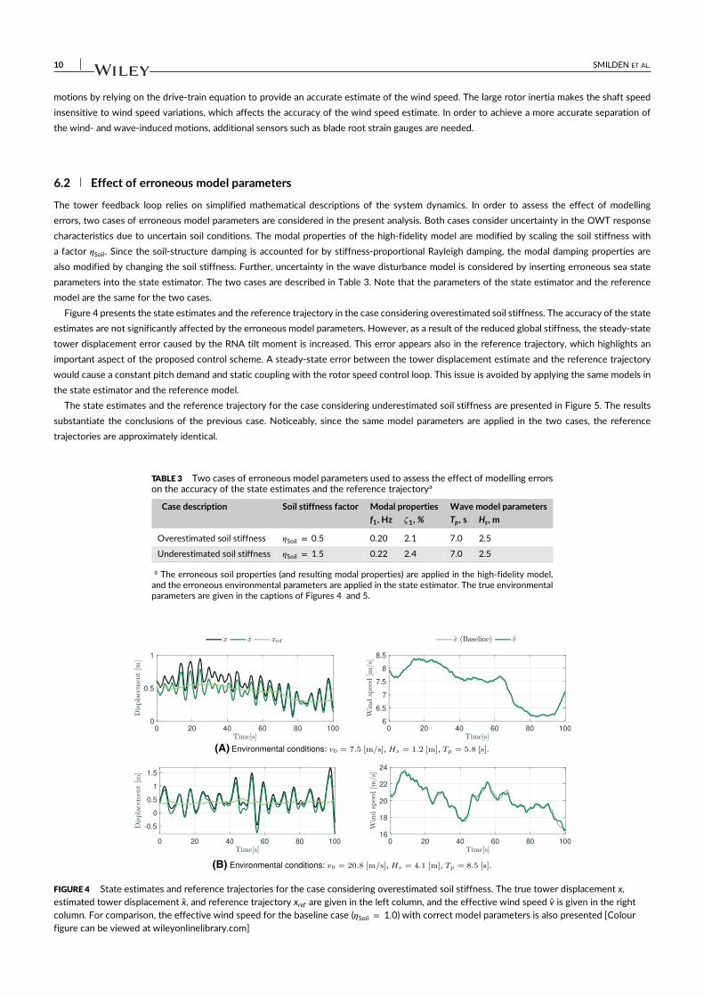
10 SMILDEN ET AL.
motions by relying on the drive-train equation to provide an accurate estimate of the wind speed. The large rotor inertia makes the shaft speed
insensitive to wind speed variations, which affects the accuracy of the wind speed estimate. In order to achieve a more accurate separation of
the wind- and wave-induced motions, additional sensors such as blade root strain gauges are needed.
6.2 Effect of erroneous model parameters
The tower feedback loop relies on simplified mathematical descriptions of the system dynamics. In order to assess the effect of modelling
errors, two cases of erroneous model parameters are considered in the present analysis. Both cases consider uncertainty in the OWT response
characteristics due to uncertain soil conditions. The modal properties of the high-fidelity model are modified by scaling the soil stiffness with
a factor 𝜂Soil. Since the soil-structure damping is accounted for by stiffness-proportional Rayleigh damping, the modal damping properties are
also modified by changing the soil stiffness. Further, uncertainty in the wave disturbance model is considered by inserting erroneous sea state
parameters into the state estimator. The two cases are described in Table 3. Note that the parameters of the state estimator and the reference
model are the same for the two cases.
Figure 4 presents the state estimates and the reference trajectory in the case considering overestimated soil stiffness. The accuracy of the state
estimates are not significantly affected by the erroneous model parameters. However, as a result of the reduced global stiffness, the steady-state
tower displacement error caused by the RNA tilt moment is increased. This error appears also in the reference trajectory, which highlights an
important aspect of the proposed control scheme. A steady-state error between the tower displacement estimate and the reference trajectory
would cause a constant pitch demand and static coupling with the rotor speed control loop. This issue is avoided by applying the same models in
the state estimator and the reference model.
The state estimates and the reference trajectory for the case considering underestimated soil stiffness are presented in Figure 5. The results
substantiate the conclusions of the previous case. Noticeably, since the same model parameters are applied in the two cases, the reference
trajectories are approximately identical.
TABLE 3 Two cases of erroneous model parameters used to assess the effect of modelling errorson the accuracy of the state estimates and the reference trajectorya
Case description Soil stiffness factor Modal properties Wave model parameters
f1, Hz 𝜁1, % Tp, s Hs, m
Overestimated soil stiffness 𝜂Soil = 0.5 0.20 2.1 7.0 2.5
Underestimated soil stiffness 𝜂Soil = 1.5 0.22 2.4 7.0 2.5
a The erroneous soil properties (and resulting modal properties) are applied in the high-fidelity model,and the erroneous environmental parameters are applied in the state estimator. The true environmentalparameters are given in the captions of Figures 4 and 5.
FIGURE 4 State estimates and reference trajectories for the case considering overestimated soil stiffness. The true tower displacement x,estimated tower displacement x, and reference trajectory xref are given in the left column, and the effective wind speed v is given in the rightcolumn. For comparison, the effective wind speed for the baseline case (𝜂Soil = 1.0) with correct model parameters is also presented [Colourfigure can be viewed at wileyonlinelibrary.com]

SMILDEN ET AL. 11
FIGURE 5 State estimates and reference trajectories for the case considering underestimated soil stiffness. The true tower displacement x,estimated tower displacement x, and reference trajectory xref are given in the left column, and the effective wind speed v is given in the rightcolumn. For comparison, the effective wind speed for the baseline case (𝜂Soil = 1.0) with correct model parameters is also presented [Colourfigure can be viewed at wileyonlinelibrary.com]
The sea state parameters applied in the state estimator deviate significantly from the true sea state parameters. Consequently, the reduced-order
wave model yields a crude approximation of the wave spectrum applied in the high-fidelity model. It is clear that accurate information about the sea
state is not required. Still, some scheduling of the model parameters based on the peak period and the significant wave height may be beneficial.
7 REDUCED-ORDER LINEAR ANALYSIS
The closed loop properties of the proposed control scheme are analysed in the following. First, the robustness of the rotor speed controller is
analysed. Then, the closed loop performance in terms of disturbance rejection capabilities and control effort is assessed. Finally, the support
structure's closed loop modal properties are analysed.
The analysis is based on the linearized low-fidelity model. Since the stochastic wind and wave models do not directly affect the closed
loop properties of the system, they are omitted from the analysis. Several publications have addressed the question of which degrees of
freedom are needed to accurately predict the response of wind turbines to control actions and disturbances.24,56,57 The present analysis is
concerned with the response characteristics in the wave frequency range. In this frequency range, the rigid drive-train mode and the first
fore-aft tower mode are of primary importance.24 As concluded by Tibaldi et al,57 the low-pass filter on the shaft speed measurement should
also be included in the analysis. In addition, dynamic inflow is accounted for, although with a reduced-order model. The applied model fidelity
is appropriate for analysing the closed loop properties of the proposed control scheme. However, including also degrees of freedom, such as
blade flexibilities, drive-train torsion, the first side-side tower mode, and a higher-order dynamic inflow model, may improve the accuracy of
the results.24,56,57 The estimates presented here, particularly the robustness estimates, should therefore be interpreted as indicative of the
true values.
Some characteristic functions need to be established for the present analysis. The open loop dynamics of the system is given by
L(s) = G(s)C(s), (19)
where the transfer function G(s) describes the frequency response of the process and the transfer function C(s) describes the frequency response
of the controller. Further, the sensitivity function S(s) and the complementary sensitivity function T(s) are defined as functions of the open loop
dynamics:
S(s) = 11 + L(s)
, T(s) = L(s)1 + L(s)
. (20)
Several properties of closed loop systems may be identified based on the sensitivity function and the complementary sensitivity function.58 The
present work is mainly concerned with properties related to robustness and disturbance rejection.
The analyses consider two sets of control parameters in the tower feedback controller. The two cases are presented in Table 4. In TFC 1,
tower feedback control with damping only is considered. In TFC 2, tower feedback control with damping and stiffness is considered. Operation
without tower feedback control is referred to as the baseline case.

12 SMILDEN ET AL.
TABLE 4 The two sets of control parameters considered in the analysesa
Case Description RSC parameters TFC parameters Modal properties
K𝝎I ,
radrad
K𝝎P ,
radsrad
fco, Hz KxP,
Nm
KxD,
Nsm
fx, Hz 𝜁x, %
TFC 1 Damping only 0.15 0.7 0.2 … 0.4 × 10⁶ 0.21 0.25
TFC 2 Damping and stiffness 0.15 0.7 0.2 0.5 × 10⁶ 0.3 × 10⁶ 0.25 0.20
a The rotor speed controller (RSC) is specified by the integral gain K𝜔I
, the proportional gain K𝜔P
, and the cut-offfrequency of the low-pass filter on the shaft speed measurement fco . The tower feedback controller (TFC) isspecified by the derivative gain Kx
Dand the proportional gain Kx
P. The approximate closed loop modal damping
ratio 𝜁x and fore-aft frequency fx are also presented.
7.1 Robustness of the rotor speed control loop
The aim of the present analysis is to analyse the influence of the tower feedback loop on the robustness of the rotor speed control loop.
Robustness is a measure of the insensitivity of the closed loop system to variations in the system parameters.58 Robustness is important to
consider because the control system is designed based on linearized models which approximate the behaviour of the non-linear system around
an operating point. The non-linearities are compensated by scheduling of the controller gains based on the collective pitch angle. Gain scheduling
based on a single variable yields a crude approximation of the true operation point which often deviates from the steady-state trajectory used to
design the controller.52
Similar to Mirzaei et al,52 the sensitivity function and complementary sensitivity function is applied to assess the robustness of the rotor speed
controller. The analysis is based on the linearized low-fidelity model with the tower feedback loop closed, meaning that it is included as part of
the system dynamics G(s). The transfer function C(s) describes the response of the rotor speed controller including the second-order low-pass
filter on the shaft speed measurement.9
The robustness of closed loop systems is often characterized by means of Nyquist's stability criterion, which is based on a graphic representation
of the open loop transfer function in a so-called Nyquist plot. Nyquist's stability criterion requires the Nyquist curve of a open loop stable system
to be to the right of the critical point −1 in the Nyquist plot. The closeness of the Nyquist curve to the critical point yields the margin of stability
for the system. In order to ensure stability in all operational conditions, sufficient stability margin is required. A measure of the stability margin
is the shortest distance dmin from the Nyquist curve to the critical point, which is given by the reciprocal of the maximum of the sensitivity
function
dmin = 1MS
, MS = maxs
|S(s)|. (21)
Small MS indicates sufficient stability margin, and a reasonable value is in the range 1.25 to 2.0.58
A different measure of robustness, also emerging from Nyquist's stability criterion, is the condition for stability under variations in the system
dynamics. This condition ensures that the Nyquist curve does not reach the critical point given a perturbation in the system dynamics from G(s)to G(s) + 𝛥G(s). Expressed as a function of the maximum of the complementary sensitivity function, the condition for stability is given by
||||ΔG(s)G(s)
|||| <1
MT, MT = max
s|T(s)|. (22)
Similar to MS , it is desirable with small values for MT, typically in the range 1.0 to 2.0.58
The maximum sensitivities MS and MT are presented in Figure 6 as functions of the tower feedback controller gains. Without tower feedback
control, the maximum sensitivities are approximately within the range 1 to 2. The aerodynamic damping of the rotor speed control mode
increases as a function of wind speed. Consequently, better robustness is achieved at higher wind speeds. The two robustness measures have
similar behaviour. For a given proportional gain, the robustness is negatively affected by increasing the derivative gain. For a given derivative
gain, the robustness is improved by increasing the proportional gain below some threshold value. Above this threshold, the robustness decreases
with increasing proportional gain.
The threshold for which increased active tower stiffness negatively affects the rotor speed controller's robustness depends on multiple
parameters. The natural frequency and damping ratio of the rotor speed control mode are determined by the integral and proportional action
on the shaft speed error, respectively. Active tower damping has a similar effect on the rotor speed control mode as reducing the proportional
action on the shaft speed error. Likewise, the effect of active tower stiffness is similar to reducing the integral action. The natural frequency
of the rotor speed control mode is therefore reduced as a function of the proportional gain in the tower feedback loop. Furthermore, the
low-pass filter in the reference model prevents rotor speed disturbances from appearing in the reference trajectory. The trend reversal in the
robustness estimates occurs when the natural frequency of the rotor speed control mode falls sufficiently below the cut-off frequency of this
low-pass filter.
The controller gains for the two cases in Table 4 are indicated in the plots. For the lower wind speed, the robustness is reduced in both TFC 1
and TFC 2. For the higher wind speed, the robustness is significantly reduced in TFC 1, while only marginally affected in TFC 2. There are some

SMILDEN ET AL. 13
FIGURE 6 Maximum values of the sensitivity function MS = maxs|S(s)| and the complementary sensitivity function MT = maxs|T(s)| as a functionof the tower feedback controller gains. Low maximum sensitivities imply high robustness, and vice versa. Wind speeds V = 12 m/s andV = 20 m/s are considered, and the red stars indicate the controller gains in the two cases presented in Table 4 [Colour figure can be viewed atwileyonlinelibrary.com]
instances where the maximum sensitivities MS are outside the preferred range between 1.25 and 2.0. However, initial investigations with the
high-fidelity model show no indications of stability issues.
The main conclusion of the present analysis is that whereas the robustness of the rotor speed controller is consistently reduced with active
tower damping, it is, within certain boundaries, improved with active tower stiffness. Active tower stiffness thereby provides leeway with respect
to robustness issues emerging from tower feedback control. Consequently, tower feedback control may be implemented without penalty to the
disturbance rejection capabilities of the rotor speed controller.
7.2 Closed loop performance
The performance of the proposed control scheme in terms of disturbance rejection and control effort is considered in the present analysis.
The sensitivity function S(s) describes the frequency response of the closed loop system to external disturbances. When plotted as a function
of frequency, the magnitude of the sensitivity function can therefore be used to analyse the disturbance rejection capabilities of the closed
loop system. Efficient disturbance rejection is expected at frequencies with magnitudes sufficiently below 0 dB. Correspondingly, amplification
of external disturbances is expected at frequencies with magnitudes above 0 dB. In a similar manner, the magnitude of the control sensitivity
function U(s) can be used to analyse the control effort for the closed loop system.59 Large magnitudes indicate that large amounts of control
effort are required, and vice versa. Thus, when analysed together with the sensitivity function, the control sensitivity function can be employed
to assess the trade-off between disturbance rejection and control effort.
Similar to the robustness analysis, the sensitivity of the rotor speed control loop is analysed with the tower feedback controller included as part
of the system dynamics. Likewise, the rotor speed controller and the low-pass filter on the shaft speed measurement are included as part of the
system dynamics when the sensitivity of the tower feedback loop is analysed. The control sensitivity is analysed by considering the closed loop
system as a single-input and multiple-output system. The magnitude of the control sensitivity function thereby indicates the combined control
effort of the two control loops. A simple two-loop system can be formulated by incorporating the reference model and its effect in terms of pitch
activity into the system dynamics G(s). In effect, the control sensitivity function does not capture the control effort contribution of the reference
model. This contribution is, however, of minor importance to the overall control effort.
The magnitude of the tower feedback sensitivity and control sensitivity function is plotted together with the lifetime probability distribution of
wave peak frequency in Figure 7. With active tower stiffness, there is a distinct improvement in the disturbance rejection capabilities in the wave
frequency range. This is, however, only the case at frequencies below the first fore-aft modal frequency. Above this frequency, the sensitivity
and control sensitivity function both favour active tower damping only. Comparing the results for the two wind speeds, higher control effort and
less efficient disturbance rejection is expected in a frequency range around 0.1 Hz for higher wind speeds. The natural frequency of the rotor
speed control mode increases slightly with the wind speed. Therefore, the interaction with the rotor speed control loop is more pronounced for
the higher wind speed.

14 SMILDEN ET AL.
(A)
(C)
(B)
(D)
FIGURE 7 Magnitude of the tower displacement sensitivity and control sensitivity function together with the lifetime probability distribution ofwave peak frequency. The two cases in Table 4 are considered, and the results are presented for two wind speeds V = 12 m/s and V = 20 m/s.The dashed lines indicate the first fore-aft modal frequency f1 [Colour figure can be viewed at wileyonlinelibrary.com]
FIGURE 8 Magnitude of the rotor speed sensitivity and control sensitivity function for wind speeds V = 12 m/s and V = 20 m/s. The baselinecase and the two cases in Table 4 are considered. The dashed lines indicate the first fore-aft modal frequency f1 [Colour figure can be viewed atwileyonlinelibrary.com]
Figure 8 presents the magnitude of the rotor speed sensitivity and control sensitivity function. Tower feedback control degrades disturbance
rejection in a frequency range around 0.1 Hz. While this effect is most pronounced with active tower damping, it occurs at frequencies closer to
the frequencies of turbulent wind variations with active tower stiffness. In any case, this performance degradation primarily occurs in a frequency
range above the frequencies of significant turbulent wind variations. Notably, even in the baseline case, rotor speed disturbances are amplified
in the wave frequency range. The cut-off frequency of the low-pass filter on the shaft speed measurement is set to 0.2 Hz, which is below the
support structure's modal frequencies, but above the frequencies of significant wave disturbances. Moreover, in order to highlight the effects of
interaction with the tower feedback loop, a set of moderately high gains is applied in the rotor speed controller. Nevertheless, simulations with
the high-fidelity model suggest that a reasonable overall performance is achieved with the selected control parameters.

SMILDEN ET AL. 15
FIGURE 9 The support structure's closed loop damping ratio and natural frequency as functions of the tower feedback controller gains. Windspeeds V = 12 m/s and V = 20 m/s are considered, and the red stars indicate the controller gains in the two cases presented in Table 4 [Colourfigure can be viewed at wileyonlinelibrary.com]
7.3 Closed loop modal properties
The support structure's closed loop modal properties with the tower feedback loop are analysed in the following. The analysis is performed with
the rotor speed controller and the low-pass filter on the shaft speed measurement included as part of the system dynamics G(s). Furthermore,
the reference model, and its effect in terms of pitch activity, is included in the description of the system dynamics. The transfer function C(s)describes the response of the tower feedback controller. Since the complementary sensitivity function T(s) is the transfer function of the closed
loop system, the modal properties are given by the poles of the complementary sensitivity function.
The closed loop damping ratio and natural frequency are presented in Figure 9 as functions of the tower feedback controller gains. As expected,
the natural frequency and the damping ratio are increased as a result of the tower feedback loop. The damping ratio is inversely proportional
to the square root of the modal stiffness. Therefore, the damping ratio is reduced as a function of the proportional gain. Furthermore, due to
coupling with the rotor speed controller, the natural frequency increases for increasing derivative gain.
8 LIFETIME ANALYSIS
The lifetime effects of the proposed control scheme are analysed in the following. First, the trade-off between the support structure's fatigue
loads and adverse side effects in the pitch actuators is analysed. Then the lifetime effects of the proposed control scheme are assessed.
8.1 Trade-off with respect to the pitch actuators
The trade-off between fatigue loads in the support structure and adverse side effects in the pitch actuators is considered here. The two cases
in Table 4 are compared with the baseline case in Figure 10. In both cases, the support structure's fatigue loads are reduced; however, the best
choice of tower feedback controller is seen to depend on the environmental conditions.
In the partial load region, active tower damping yields the largest reduction in the support structure's fatigue loads. Low and moderate wind
speeds are correlated with sea states with peak frequency close to the fore-aft modal frequency. The power spectral density of the fore-aft
nacelle displacement is presented in Figure 11A. In the baseline case, the response is restricted to a comparatively narrow frequency range around
the modal frequency. The proportional-derivative controller relocates the wave response to the frequency range predicted by the reduced-order
linear analysis. Relocating the closed loop modal frequency away from the excitation frequencies reduces dynamic amplification. Still, increasing
the damping is more effective for reducing the response amplitudes.
In the full load region, tower feedback control with proportional-derivative action yields the largest reduction in the support structure's fatigue
loads. In the most severe environmental conditions, the fatigue damage is reduced by approximately 80% in TFC 2. In TFC 1, the fatigue damage
is only reduced by approximately 10% to 30% in the same environmental conditions. Since high wind speeds are correlated with severe sea
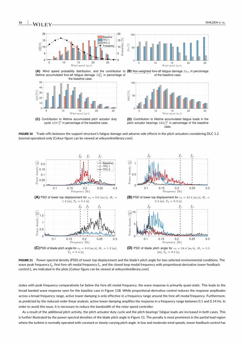
16 SMILDEN ET AL.
FIGURE 10 Trade-offs between the support structure's fatigue damage and adverse side effects in the pitch actuators considering DLC 1.2(normal operation) only [Colour figure can be viewed at wileyonlinelibrary.com]
FIGURE 11 Power spectral density (PSD) of tower top displacement and the blade's pitch angle for two selected environmental conditions. Thewave peak frequency fp , first fore-aft modal frequency f1, and the closed loop modal frequency with proportional-derivative tower feedbackcontrol fx are indicated in the plots [Colour figure can be viewed at wileyonlinelibrary.com]
states with peak frequency comparatively far below the fore-aft modal frequency, the wave response is primarily quasi-static. This leads to the
broad banded wave response seen for the baseline case in Figure 11B. While proportional-derivative control reduces the response amplitudes
across a broad frequency range, active tower damping is only effective in a frequency range around the fore-aft modal frequency. Furthermore,
as predicted by the reduced-order linear analysis, active tower damping amplifies the response in a frequency range between 0.1 and 0.14 Hz. In
order to avoid this issue, it is necessary to reduce the bandwidth of the rotor speed controller.
As a result of the additional pitch activity, the pitch actuator duty cycle and the pitch bearings' fatigue loads are increased in both cases. This
is further illustrated by the power spectral densities of the blade pitch angle in Figure 11. The penalty is most prominent in the partial load region
where the turbine is normally operated with constant or slowly-varying pitch angle. In low and moderate wind speeds, tower feedback control has
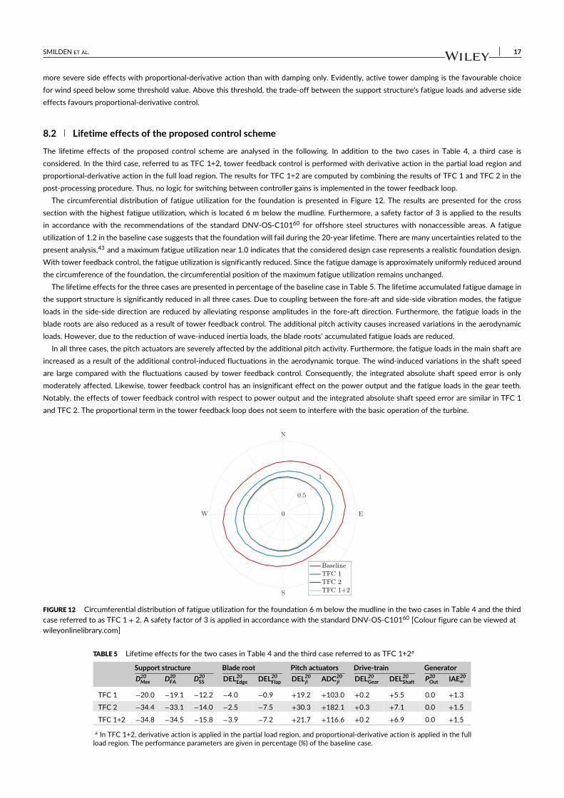
SMILDEN ET AL. 17
more severe side effects with proportional-derivative action than with damping only. Evidently, active tower damping is the favourable choice
for wind speed below some threshold value. Above this threshold, the trade-off between the support structure's fatigue loads and adverse side
effects favours proportional-derivative control.
8.2 Lifetime effects of the proposed control scheme
The lifetime effects of the proposed control scheme are analysed in the following. In addition to the two cases in Table 4, a third case is
considered. In the third case, referred to as TFC 1+2, tower feedback control is performed with derivative action in the partial load region and
proportional-derivative action in the full load region. The results for TFC 1+2 are computed by combining the results of TFC 1 and TFC 2 in the
post-processing procedure. Thus, no logic for switching between controller gains is implemented in the tower feedback loop.
The circumferential distribution of fatigue utilization for the foundation is presented in Figure 12. The results are presented for the cross
section with the highest fatigue utilization, which is located 6 m below the mudline. Furthermore, a safety factor of 3 is applied to the results
in accordance with the recommendations of the standard DNV-OS-C10160 for offshore steel structures with nonaccessible areas. A fatigue
utilization of 1.2 in the baseline case suggests that the foundation will fail during the 20-year lifetime. There are many uncertainties related to the
present analysis,43 and a maximum fatigue utilization near 1.0 indicates that the considered design case represents a realistic foundation design.
With tower feedback control, the fatigue utilization is significantly reduced. Since the fatigue damage is approximately uniformly reduced around
the circumference of the foundation, the circumferential position of the maximum fatigue utilization remains unchanged.
The lifetime effects for the three cases are presented in percentage of the baseline case in Table 5. The lifetime accumulated fatigue damage in
the support structure is significantly reduced in all three cases. Due to coupling between the fore-aft and side-side vibration modes, the fatigue
loads in the side-side direction are reduced by alleviating response amplitudes in the fore-aft direction. Furthermore, the fatigue loads in the
blade roots are also reduced as a result of tower feedback control. The additional pitch activity causes increased variations in the aerodynamic
loads. However, due to the reduction of wave-induced inertia loads, the blade roots' accumulated fatigue loads are reduced.
In all three cases, the pitch actuators are severely affected by the additional pitch activity. Furthermore, the fatigue loads in the main shaft are
increased as a result of the additional control-induced fluctuations in the aerodynamic torque. The wind-induced variations in the shaft speed
are large compared with the fluctuations caused by tower feedback control. Consequently, the integrated absolute shaft speed error is only
moderately affected. Likewise, tower feedback control has an insignificant effect on the power output and the fatigue loads in the gear teeth.
Notably, the effects of tower feedback control with respect to power output and the integrated absolute shaft speed error are similar in TFC 1
and TFC 2. The proportional term in the tower feedback loop does not seem to interfere with the basic operation of the turbine.
FIGURE 12 Circumferential distribution of fatigue utilization for the foundation 6 m below the mudline in the two cases in Table 4 and the thirdcase referred to as TFC 1 + 2. A safety factor of 3 is applied in accordance with the standard DNV-OS-C10160 [Colour figure can be viewed atwileyonlinelibrary.com]
TABLE 5 Lifetime effects for the two cases in Table 4 and the third case referred to as TFC 1+2a
Support structure Blade root Pitch actuators Drive-train Generator
D20Max D20
FA D20SS DEL20
Edge DEL20Flap DEL20
𝜷 ADC20𝜷 DEL20
Gear DEL20Shaft P20
Out IAE20𝝎
TFC 1 −20.0 −19.1 −12.2 −4.0 −0.9 +19.2 +103.0 +0.2 +5.5 0.0 +1.3
TFC 2 −34.4 −33.1 −14.0 −2.5 −7.5 +30.3 +182.1 +0.3 +7.1 0.0 +1.5
TFC 1+2 −34.8 −34.5 −15.8 −3.9 −7.2 +21.7 +116.6 +0.2 +6.9 0.0 +1.5
a In TFC 1+2, derivative action is applied in the partial load region, and proportional-derivative action is applied in the fullload region. The performance parameters are given in percentage (%) of the baseline case.
18 SMILDEN ET AL.
The lifetime effects of tower feedback control, both desirable and undesirable, are generally more pronounced with proportional-derivative
action. Tower feedback control with damping in the partial load region and proportional-derivative action in the full load region yields the most
favourable trade-off between the support structure's fatigue damage and adverse side effects. In this case, the adverse side effects are of similar
severity as with conventional active tower damping, while the support structure's fatigue life is further improved.
9 CONCLUSIONS
In this paper, a control scheme for reducing the wave-induced fatigue loads in monopile OWT support structures was proposed. The control
scheme applied collective pitch control to increase both the damping and stiffness of the support structure's fore-aft vibration modes. The
design case was a 10-MW wind turbine located in 30-m water depth at the Dogger Bank in the North Sea. The proposed control scheme was
model-based in the sense that it included a state estimator and a reference model. A low-fidelity offshore wind turbine model, including a wave
disturbance model, was therefore established. The state estimator and the reference model were verified based on time-domain simulations with
a high-fidelity offshore wind turbine model in an aero-hydro-servo-elastic simulation tool. Furthermore, based on the low-fidelity model, the
closed loop properties of the proposed control scheme were analysed and compared with conventional active tower damping. Finally, based on
time-domain simulations with the high-fidelity model, the lifetime effects of the proposed control scheme were analysed.
The tower displacement estimates closely matched the true tower displacements of the high-fidelity model. However, a steady-state
displacement error caused by the unmodelled tilt moment from the rotor-nacelle assembly was observed. Since the same models were applied
in the state estimator and the reference model, this error also appeared in the reference trajectory. Therefore, the steady-state error did not
negatively affect the performance of the proposed control scheme. As a result of the wave disturbance model, it was possible to achieve
accurate displacement estimates without wave disturbances in the wind speed estimates. Furthermore, the accuracy of the state estimates and
the reference trajectory was not significantly affected by erroneous model parameters, such as the soil stiffness and the sea state parameters.
Closed loop analysis with the low-fidelity model showed that conventional active tower damping consistently reduces the robustness of the
rotor speed control loop. With active tower stiffness, the robustness was improved within certain boundaries. Consequently, it was possible to
implement tower feedback control without reducing the bandwidth of the rotor speed control loop. Furthermore, with the proposed control
scheme, efficient wave disturbance rejection could be achieved across a broad frequency range. With conventional active tower damping,
efficient disturbance rejection was restricted to a narrow frequency range around the first fore-aft modal frequency.
The results of the time-domain simulations with the high-fidelity model confirmed the closed loop behaviour predicted by the low-fidelity
model. In the partial load region, active tower damping gave the largest fatigue load reduction for the support structure. Conversely, in the full
load region, tower feedback control with stiffness and damping gave the largest fatigue load reduction. The pitch actuators and the main shaft
were severely affected by the additional pitch activity. Other performance measures, such as blade root fatigue loads, gearbox fatigue loads,
and shaft speed variability, were either improved or marginally affected. The power output was not affected in any of the simulation cases. The
most favourable trade-off between adverse side effects and the support structure's fatigue loads was achieved with active tower damping in the
partial load region and active tower damping and stiffness in the full load region. In this case, the adverse side effects were of similar severity as
with conventional active tower damping, while the support structure's fatigue life was further improved.
ACKNOWLEDGEMENTS
This work has been carried out at the Centre for Autonomous Marine Operations and Systems (NTNU AMOS). The Norwegian Research Council
is acknowledged as the main sponsor of NTNU AMOS. This work was supported by the Research Council of Norway through the Centres of
Excellence funding scheme, project number 223254—NTNU AMOS.
ORCID
Emil Smilden http://orcid.org/0000-0001-8547-9353
Erin E. Bachynski http://orcid.org/0000-0002-1471-8254
REFERENCES
1. Ho A, Mbistrova A. The European offshore wind industry—Key trends and statistics 2016. EWEA, Brussels, Belgium; 2017.
2. Fischer T, Vries W, Rainey P, Schmidt B, Argyriadis K, Kühn M. Offshore support structure optimization by means of integrated design and controls.Wind Energy. 2012;15(1):99-117.
3. Smilden E, Bachynski E, Sørensen A. Key contributors to lifetime accumulated fatigue damage in an offshore wind turbine support structure. In: ASME2017 36th International Conference on Ocean, Offshore and Arctic Engineering. American Society of Mechanical Engineers; 2017:V010T09A075,Trondheim, Norway.
4. Fischer T. Mitigation of aerodynamic and hydrodynamic induced loads of offshore wind turbines. Shaker, University of Stuttgart; 2012.
5. Van der Hooft E, Schaak P, Van Engelen T. Wind turbine control algorithms. Technical Report DOWEC-F1W1-EH-03-094/0, Delft, TheNetherlands, Energy Research Center of the Netherlands (ECN); 2003.
SMILDEN ET AL. 19
6. Bossanyi E. Wind turbine control for load reduction. Wind energy. 2003;6(3):229-244.
7. Bossanyi E, Ramtharan G, Savini B. The importance of control in wind turbine design and loading. In: 17th Mediterranean Conference on Control andAutomation, 2009. MED'09. Thessaloniki, Greece: IEEE; 2009:1269-1274.
8. Fischer B, Shan M. A survey on control methods for the mitigation of tower loads. IWES Project report 01/104256, Fraunhofer-Institute for WindEnergy and Energy Systems Technology; 2013.
9. Hansen MH, Henriksen LC. Basic DTU wind energy controller. Technical Report, DTU Wind Energy; 2013. Report nr: 0028.
10. Jonkman J, Butterfield S, Musial W, Scott G. Definition of a 5-MW reference wind turbine for offshore system development. Technical Report,Golden, CO., National Renewable Energy Laboratory (NREL); 2009. Report nr: NREL/TP-500-38060.
11. Leithead WE, Dominguez S. Coordinated control design for wind turbine control systems. In: Proceedings of European Wind Energy Conference andExhibition, Vol. 27; 2006; Athens, Greece.
12. Leithead W, Dominguez S. Controller design for the cancellation of the tower fore-aft mode in a wind turbine. In: 44th IEEE Conference on Decisionand Control, 2005 and 2005 European Control Conference. CDC-ECC'05. Seville, Spain: IEEE; 2005:1276-1281.
13. Fischer B. Reducing rotor speed variations of floating wind turbines by compensation of non-minimum phase zeros. IET Renew Power Gener.2013;7(4):413-419.
14. Larsen TJ, Hanson TD. A method to avoid negative damped low frequent tower vibrations for a floating, pitch controlled wind turbine. Journal ofPhysics: Conference Series, Vol. 75. Copenhagen, Denmark: IOP Publishing; 2007:012073.
15. Li L, Gao Z, Moan T. Joint distribution of environmental condition at five European offshore sites for design of combined wind and wave energydevices. J Offshore Mech Arct Eng. 2015;137(3):031901.
16. Henriksen LC. Model predictive control of wind turbines. Ph.D. Thesis. Lyngby, Denmark: Technical University of Denmark, DTU, DK-2800 Kgs; 2010.
17. Mirzaei M, Poulsen NK, Niemann HH. Robust model predictive control of a wind turbine. In: American Control Conference (ACC), 2012 IEEE;2012:4393-4398; Montreal, Canada.
18. Evans MA, Cannon M, Kouvaritakis B. Robust MPC tower damping for variable speed wind turbines. IEEE Trans Control Syst Technol.2015;23(1):290-296.
19. Christiansen S, Tabatabaeipour SM, Bak T, Knudsen T. Wave disturbance reduction of a floating wind turbine using a reference model-based predictivecontrol. In: American Control Conference (ACC), 2013 IEEE; 2013:2214-2219; Washington DC, United States.
20. Christiansen S, Bak T, Knudsen T. Damping wind and wave loads on a floating wind turbine. Energies. 2013;6(8):4097-4116.
21. Namik H, Stol K. Individual blade pitch control of floating offshore wind turbines. Wind Energy. 2010;13(1):74-85.
22. Knudsen T, Bak T, Soltani M. Prediction models for wind speed at turbine locations in a wind farm. Wind Energy. 2011;14(7):877-894.
23. Henriksen LC, Hansen MH, Poulsen NK. A simplified dynamic inflow model and its effect on the performance of free mean wind speed estimation.Wind Energy. 2013;16(8):1213-1224.
24. Sønderby I, Hansen MH. Open-loop frequency response analysis of a wind turbine using a high-order linear aeroelastic model. Wind Energy.2014;17(8):1147-1167.
25. Carswell W, Arwade SR, DeGroot DJ, Lackner MA. Soil–structure reliability of offshore wind turbine monopile foundations. Wind Energy.2015;18(3):483-498.
26. Damgaard M, Andersen LV, Ibsen LB, Toft HS, Sørensen JD. A probabilistic analysis of the dynamic response of monopile foundations: Soil variabilityand its consequences. Probab Eng Mech. 2015;41:46-59.
27. Schafhirt S, Page A, Eiksund GR, Muskulus M. Influence of soil parameters on the fatigue lifetime of offshore wind turbines with monopile supportstructure. Energy Procedia. 2016;94:347-356.
28. Devriendt C, Jordaens PJ, De Sitter G, Guillaume P. Damping estimation of an offshore wind turbine on a monopile foundation. IET Renew PowerGener. 2013;7(4):401-412.
29. Damgaard M, Ibsen LB, Andersen LV, Andersen JK. Cross-wind modal properties of offshore wind turbines identified by full scale testing. J Wind EngInd Aerodyn. 2013;116:94-108.
30. Hansen MH, Thomsen K, Fuglsang P, Knudsen T. Two methods for estimating aeroelastic damping of operational wind turbine modes fromexperiments. Wind Energy. 2006;9(1-2):179-191.
31. Sørensen NN, Madsen HA. Modelling of transient wind turbine loads during pitch motion. In: Proceedings of the European Wind Energy Conferenceand Exhibition, Athens, Greece; 2006; Athens, Greece.
32. Van Engelen T, Van Der Hooft E. Dynamic inflow compensation for pitch controlled wind turbines. In: Proceedings EWEA Conference; 2004;London:22-25.
33. Knudsen T., Bak T.. Simple model for describing and estimating wind turbine dynamic inflow. In: American Control Conference (ACC), 2013 IEEE;2013:640-646; Washington DC, United States.
34. Øye S. Unsteady wake effects caused by pitch–angle changes. In: 1st Symposium on IEA R&D WECS Joint Action on Aerodynamics of Wind Turbines;1986; London, UK:58-79.
35. Hansen MO. Aerodynamics of Wind Turbines. New York: Routledge; 2015.
36. Faltinsen O. Sea Loads on Ships and Offshore Structures. Cambridge, United Kingdom: Cambridge university press; 1993.
37. MacCamy R, Fuchs RA. Wave forces on piles: a diffraction theory. Technical Report, DTIC Document; 1954. Report nr: NTIS AD 699 406.
38. Hespanha JP. Linear Systems Theory. Princeton New Jersey, United States: Princeton University Press; 2009.
39. Sørensen P, Hansen AD, Rosas PAC. Wind models for simulation of power fluctuations from wind farms. J Wind Eng Ind Aerodyn. 2002;90(12):1381-1402.
40. groupDNV GL. DNV-RP-C205. Environmental conditions and environmental loads; 2010.
41. Fossen TI. Handbook of Marine Craft Hydrodynamics and Motion Control. West Sussex, United Kingdom: John Wiley & Sons; 2011.

20 SMILDEN ET AL.
42. Brown RG, Hwang PY. Introduction to random signals and applied Kalman filtering. New York, United States: John Wiley & Sons; 2012:c1997.
43. Smilden E, Bachynski EE, Sørensen AJ, Amdahl J. Site-specific controller design for monopile offshore wind turbines. Mar Struct. 2018;61:503-523.
44. DNV GL. Loads and site conditions for wind turbines. DNVGL-ST-0437; 2016.
45. Bak C, Zahle F, Bitsche R, et al. Description of the DTU 10 MW reference wind turbine. DTU Wind Energy, Risø, Denmark; Report-I-0092; 2013.
46. Ormberg H, Bachynski EE. Global analysis of floating wind turbines: code development, model sensitivity and benchmark study. In: The Twenty-SecondInternational Offshore and Polar Engineering Conference. Rhodes, Greece: International Society of Offshore and Polar Engineers; 2012.
47. Bachynski EE, Ormberg H. Hydrodynamic modeling of large-diameter bottom-fixed offshore wind turbines. In: ASME 2015 34th InternationalConference on Ocean, Offshore and Arctic Engineering. St. John's, Canada: American Society of Mechanical Engineers; 2015:V009T09A051.
48. Reistad M, Breivik Ø, Haakenstad H, Aarnes OJ, Furevik BR, Bidlot J-R. A high-resolution hindcast of wind and waves for the North Sea, the NorwegianSea, and the Barents Sea. J Geophys Res Oceans. 2011;116(C5):C05019.
49. International Electrotechnical Commission (IEC). IEC 61400-1: Wind turbines part 1: design requirements. Technical Report, Geneva, Switzerland;2005.
50. Jonkman BJ. Turbsim user's guide; 2009.
51. Carroll J, McDonald A, Dinwoodie I, McMillan D, Revie M, Lazakis I. Availability, operation and maintenance costs of offshore wind turbines withdifferent drive train configurations. Wind Energy. 2017;20(2):361-378.
52. Mirzaei M, Tibaldi C, Hansen MH. Pi controller design of a wind turbine: evaluation of the pole-placement method and tuning using constrainedoptimization. Journal of Physics: Conference Series, Vol. 753. Munich, Germany: IOP Publishing; 2016:052026.
53. DNV GL. Fatigue design of offshore steel structures. DNV-RP-C203; 2010.
54. Nejad AR, Gao Z, Moan T. On long-term fatigue damage and reliability analysis of gears under wind loads in offshore wind turbine drivetrains. Int JFatigue. 2014;61:116-128.
55. Niederstucke B, Anders A, Dalhoff P, Grzybowski R. Load data analysis for wind turbine gearboxes. Final Report of Enhanced Life Analysis of WindPower Systems. Hamburg, Germany: Germanicher Lloyd WindEnergie GmbH; 2003.
56. Merz KO. Basic controller tuning for large offshore wind turbines. Wind Energy Sci. 2016;1(2):153.
57. Tibaldi C, Hansen MH, Zahle F. Methods for systematic tuning of wind turbine controllers. Technical Report, DTU Wind Energy; 2015; Risø, Denmark.Report nr: 0100.
58. Åström KJ, Hägglund T. Advanced PID control. ISA-The Instrumentation, Systems and Automation Society; 2006.
59. Skogestad S, Postlethwaite I. Multivariable Feedback Control: Analysis and Design, Vol. 2. New York: Wiley; 2007.
60. DNV GL. OS-C101. Design of offshore steel structures; 2011.
How to cite this article: Smilden E, Bachynski EE, Sørensen AJ, Amdahl J. Wave disturbance rejection for monopile offshore wind
turbines. Wind Energy. 2018;1–20. https://doi.org/10.1002/we.2273
Received 26 April 2016; Revised 6 June 2016; Accepted 6 June 2016DOI: xxx/xxxx
RESEARCHARTICLE
Post-installation adaptation of offshorewind turbine controlsEmil Smilden | Stian H. Sørum | Erin E. Bachynski | Asgeir J. Sørensen | Jørgen Amdahl1Centre for AutonomousMarineOperationsand Systems (NTNUAMOS), Department ofMarine Technology, Norwegian University ofScience and Technology, Trondheim, NorwayCorrespondence*Emil Smilden, Email: [email protected] Address
AbstractThe cost of offshorewind energy canbe reducedby incorporating control strategies to reduce thesupport structures’ load effects into the structural design process.While effective in reducing thecost of support structures, load-reducing controls produce potentially costly side-effects in otherwind turbine components and subsystems. This paper proposes a methodology to mitigate theseside-effects at the wind farm level. The interaction between the foundation and the surroundingsoil is a major source of uncertainty in estimating the safety margins of support structures. Thesafety margins are generally closely correlated with the modal properties (natural frequencies,damping ratios). This admits the possibility of using modal identification techniques to reassessthe structural safety after installing and commissioning the wind farm. Since design standardsrequire conservative design margins, the post-installation safety assessment is likely to revealbetter than expected structural safety performance. Thus, if load-reducing controls have beenadopted in the structural design process, it is likely permissible to reduce the use of these dur-ing actual operation. Here, the probabilistic outcome of such a two-stage controls adaptation isanalysed. The analysis considers the structural design of a 10MW monopile offshore wind tur-bineunder uncertainty in the site-specific soil conditions. The results show that apost-installationadaptation can reduce the side-effects of load-reducing controls by up to an order of magnitudeat the wind farm level.KEYWORDS:Offshore wind energy, Structural design, Control design, Geotechnical design, Structural healthmonitoring, Structural reliability
1 INTRODUCTIONSupport structures are a major contributor to the cost of offshore wind energy. Favored for their cost-efficiency, monopile foundations are preva-lent in the European offshore wind industry 1. The support structures’ dimensions are governed by requirements regarding ultimate, serviceability,and fatigue limit states. The environmental load effects in these limit states dependon thewind turbine’s control system. It iswidely recognized thatthe fatigue load effects are governed by the global response characteristics which, in turn, depend on the turbine’s closed loop properties. Further-more, the ultimate and serviceability load effects depend on the turbine’s operational settings, such as the cut-out and ratedwind speed. A numberof control strategies are available for reducing load effects in offshore wind turbine (OWT) support structures 2,3,4,5,6,7. However, regardless of thecontrol strategy used, there are unavoidable adverse side-effects, such as wear and tear of various wind turbine components, and power outputdegradation in terms of both quality and quantity 2,7. These side-effectsmay significantly reduce or even offset the cost savings enabled by the load-reducing controls.The interaction between the foundation and the surrounding soil is a major source of uncertainty in estimating the safety margins of support
structures 8,9,10,11,12,13,14. In particular, uncertainty in the support structures’ fundamental natural frequency presents a challenge in estimating their

2 Smilden ET AL.
fatigue life. The fundamental natural frequency is usually placed in the relatively narrow “soft-stiff” frequency range in between the rotor frequency(1P), and blade passing frequency (3P) 15. Any coincidencewith the rotor excitation frequenciesmay cause a significant reduction in fatigue life. Fur-thermore, due to increasing turbine sizes, the “soft-stiff” frequency range is falling closer to thewave excitation frequencies, thusmaking fatigue lifeestimation even more sensitive to uncertainty in the fundamental natural frequency. There is also uncertainty about the magnitude of responses.This affects not only the estimation of fatigue life, but also the estimation of servicebility capacities which are defined in terms of deflections androtations (tilt) at the pile head and nacelle level 16,17. The fatigue and serviceability requirements usually lead to conservative ultimate capacities 17.Moreover, since structural collapse is caused by failure of the foundation rather than the the surrounding soil, the ultimate capacities are not verysensitive to uncertainties in the soil-structure properties 18.Althoughnot yet inwidespread commercial use, there aremanyexamples of structuralmonitoring systemshavingbeen successfully employed to
estimate themodal properties of OWT support structures 19,20,21,22,23,24,25,26,27. Structural health monitoring has typically been proposed to enableimproved life-cycle maintenance and inspection management, and early detection of deterioration phenomena, such as scouring around the foun-dation. The data collected from such monitoring systems could also be useful for making turbine-specific adjustments to the controls. Supposingthat information about the true modal properties is available, the uncertainty in the structural safety margins is reduced. Since design standardsgenerally require conservative design margins, the true modal properties are likely to reveal better than expected structural safety performance.Thus, if load-reducing controls have been adopted in the structural design process, it is likely permissible to reduce the use of these during actualoperation. This fact can be exploited by incorporating a post-installation adaptation of load-reducing controls into the structural design process.For the majority of turbines, this would lead to a win-win situation where load-reducing controls have been used to reduce the support structure’scost without having to be used in actual operation, at least not to their fullest potential.The main contribution of this paper is to propose and analyse a post-installation adaptation of control strategies for reducing the cost of OWT
support structures. The overall objective is to increase the cost-efficiency of load-reducing controls by mitigating their adverse side-effects at thewind farm level. Hence, the focus is on optimizing the use of existing control strategies rather than the development of new or improved controlstrategies. A simulation study considering the structural design of a 10MWmonopile OWT under uncertainty in the site-specific soil conditions isconducted in order to evaluate the proposed methodology. Two control strategies are considered in separate analyses: (1) tower feedback controlto increase the support structure’s fatigue life, and (2) peak shaving to increase the support structure’s serviceability capacity. The analyses are per-formed using the aero-hydro-servo-elastic simulation tool SIMA by SINTEFOcean.Thepaper is organizedas follows: First, the controls adaptationprocedure is formulatedas a two-stagedesignproblem inSection2.Next, the ran-
domfield soilmodel and the soil-structure interactionmodel are presented in Section3. Further, the simulation setup is described in Section4. Then,the selection of characteristic soil properties are discussed in Section 5. Finally, the probabilistic outcomes of the two-stage controls adaptation areanalysed in Sections 6 and 7, before the paper is concluded in Section 8.
2 BACKGROUNDANDPROBLEMFORMULATIONThe structural design of an OWT is a partially iterative process, involving both the wind turbine manufacturer and foundation designer 18,28,29.While the support structures’ dimensions are determined through an iterative process, current offshore wind projects use standard off-the-shelfrotor-nacelle assemblies that offer limitedpossibilities for project-specific adaptations.Apreliminarydesign for the rotor-nacelle assemblies (RNA),including the controls, is decided upon in the early stages of the conceptual design phase. The suitability of the rotor-nacelle assemblies is thenreassessed on the basis of the actual project-specific data during certification at the end of the structural design process 29. Fischer et al. 29 demon-strated how the conventional design process can be modified to accommodate the adaptation of control strategies to reduce the cost of supportstructures. As illustrated in Figure 1 , the methodology proposed in the present paper extends the adaptation of load reducing controls to a two-stage design problem 30. In thefirst stage, the support structures’s dimensions and initial settings for the load reducing controls are chosen based onprior information about the uncertain parameters. In the second stage, once more information becomes available regarding the uncertain param-eters, the settings for the load reducing controls are adjusted based on updated estimates of structural safety margins. A two-stage formulationis applicable to design problems for which the uncertainties are related to manufacturing, fabrication, and construction, such as uncertainty in thesite-specific soil conditions, or certain structural parameters. In the case of temporal uncertainties, such as the environmental conditions, turbineavailability, or soil erosion and degradation, a multi-stage formulation is required for describing the design problem.A general formulation of the two-stage design problem is given by
Minimizex∈X
: CS(x) + Eξ[CC(x, ξ)
]
subject to : P[Gj(x, ξ) ≤ 0
]≤ Pj, j = 1, 2, . . .m
(1)

Smilden ET AL. 3whereCC(x, ξ) is the solution of the second stage problem
Minimizey∈Y
: CC(x, y(ξ))
subject to : P[Gj(x, y(ξ)) ≤ 0
]≤ Pj, j = 1, 2, . . .m
(2)
The first stage decision variables x ∈ X governs the support structure’s dimensions and the initial settings for the load reducing controls. Therandom variables ξ are the uncertain data, which in the present case are parameters related to the soil conditions. The objective of the first stageproblem is tominimize the total of the support structure’s costCS(x) and the expected cost of the control strategies adopted to reduce the supportstructure’s load effects E
[CC(x, ξ)
]. The dimensions of the support structure are constrained by the probabilities of failure P[Gj(x, ξ) ≤ 0
]whichcannot exceed the target failure probabilities Pj. The required margin of safety must be fulfilled for all failure modes j = 1, 2, . . .m. The secondstage decision variables y ∈ Y govern the settings for the load reducing controls once the uncertain variables have unfolded. The objective of thesecond stage problem is to minimize the use of load reducing controls, while adhering to the required level of structural safety. The key feature ofthe two-stage formulation is the interdependence between the first- and second stage in the design problem. Most importantly, in the first stage,decisions should be made taking into account the probabilistic outcome of the second stage problem. Of course, the solution of the second stageproblem depends on the decisionsmade in the first stage.The two-stage controller adaptation presupposes that information about the true modal properties becomes available once the tur-
bines have been installed. There are several examples where modal identification techniques have been successfully applied to wind tur-bines 19,20,21,22,23,24,25,26,27. The modal properties are usually estimated from acceleration data collected at one or more vertical locations alongthe support structure. Collecting acceleration data at several vertical locations makes it possible to estimate the mode shapes in addition to themodal frequencies and damping ratios 23,24,25. Reassessing the structural safetymargins requires accurate and reliable information about themodalproperties. In general, the modal properties estimated at discrete time instants, for instance during rotor-stop events, are subject to considerableuncertainties 20,23,26,27. A system for continuous monitoring should therefore be employed 20,21,22,23,24,25. An example of such a monitoring systemwas developed and tested in full scale by Devriendt et al. 24. Based on data collected from an idling turbine over a two-week period, the modalproperties of five fundamental modes were identified. The applicability of the system was further proven byWeijtjens et al. 25 who employed datacollectedover a two-year period to track changes in themodal frequencies. As further explained in Section3, thepresentwork considers only uncer-tainty in themodal frequencies due to the inherent variability in the site-specific soil conditions. It is generally more difficult to obtain accurate andreliable information about the damping ratios than themodal frequencies. Furthermore, in order for the proposedmethodology to be presented ina straightforwardmanner, it is desirable to deal with only one uncertain parameter.
3 GEOTECHNICALMODELSAgeotechnical design basis is established in the following. First, the different sources of geotechnical uncertainties are discussed and the procedurefor generating random soil profiles is presented. Then, a random field model is constructed based on conditions at the Dogger Bank in the NorthSea. Finally, the soil-structure interactionmodel is presented.
3.1 Geotechnical uncertainties and random fieldmodelingSoil is a heterogeneous material with properties that vary verically and horizontally. The three primary sources of geotechnical uncertainty areinherent variability, measurement uncertainty, and transformation uncertainty 32,33,34,35. The inherent variability of the soil properties is due tonatural heterogeneity resulting from continuous geological processes. In general, this source of uncertainty cannot be reduced by collecting moredata or performing more tests 35. Measurement and transformation uncertainties emerge frommeasurement errors, statistical uncertainty due tolimited amounts of information, and the correlation models used for transforming field or laboratory measurements into engineering properties.These uncertainties depend on the quality of the equipment being used, procedural control, and the amount of data collected 32,35. In practice, theuncertainties due to measurement and transformation errors are often embedded in the inherent variability under the assumption that their con-tributions to the overall uncertainty are small 35. Furthermore, depending on the number of samples, the statistical uncertainty can be taken intoaccount in the estimation of the soil properties’ mean value 35. Hence, only the inherent soil variability is modeled in the present work.Inherent soil variability is usually modeled as random fields characterized by their mean, coefficient of variation (COV), and scale of fluctua-
tion 32,33,34. As illustrated in Fig. 2 , the spatial variability of a soil property ξ can be decomposed into a mean trend µ and a fluctuating componentw, such that
ξ(z) = µ(z) + w(z) (3)

4 Smilden ET AL.
Site-specificdesign basis
PreliminaryRNA design
Tower andRNA design
Foundationdesign
1st stage cont-rols adaptation
Design checks
OK?
Final design,verification
Conceptual design
Basic design (iterative)
Detailed design and verification
NoNo
Yes
Not specifiedControl designStructural design
Installation,commissioning
2nd stage cont-rols adaptation
Installation, commissioning, and operation
FIGURE 1 Outline of the design process for an offshore wind turbine with a two-stage adaptation of load reducing controls. The outline is basedon information presented by Seidel 28, Seidel et al 18, Fischer et al 29, and IEC 61400-3 31.
where z is the depth below the ground surface 32.Within a soil layer, themean trend is often assumed either constant, or linearly varyingwith depth.The vertical scale of fluctuation δ is the distance over which the soil property shows strong correlation. The distance δ is related to the average dis-tance between crossings of the fluctuating soil property and themean trend 32,34.It is straightforward to generate a vertical sequence of correlated random soil properties from a random field with probability distribution
Fξ(ξ)10,36,12. For each randomfield realization, a vectorU of uncorrelated standardGaussian distributed variablesUi where i = 1, 2, . . . , n is gener-
ated. The dimension n corresponds to the number of depth increments in the soil-structure interaction model. The vector Y of correlated standardGaussian distributed variablesYi is then computed by Choleski triangulation of the positive definite correlationmatrix ρ, such that
Y = TU, TTT = ρ (4)where T is the lower triangular matrix. The correlation matrix describes the vertical correlation structure of the random field, which is frequentlycharacterized by autocorrelation functions. Such functions describe the correlation between two points based on their vertical separation distance(lag) and the vertical scale of fluctuation 34. Finally, the vertical sequence ξ of correlated random soil properties ξi can be computed by applying thecomponentwise transformation given by
ξi = F−1ξ
(Φ(Yi)
), i = 1, 2, . . . , n (5)
whereΦ(Yi) is the standard Gaussian probability distribution.
3.2 Random fieldmodelAwind farm site at theDogger Bank in theNorth Sea is used as a basis for establishing the random fieldmodel. The soil profile at the design locationconsists of a surface layer of dense sand with underlying layers of stiff clays. Based on these soil conditions, a simple three-layered random fieldmodel is constructed. For geotechnical design in clay, the submerged unit weight γ and undrained shear strength su are typical parameters usedto describe the mechanical behaviour of soil. Likewise, the mechanical behaviour of sand is described by the submerged unit weight and angle of

Smilden ET AL. 5
Seabed
Layer 1 Scale of fluctuation δ
Layer 2 Soil property ξ(z)
Layer 3
Mean µ(z)
Fluctuationw(z)
FIGURE 2 Random fieldmodel (Adapted from Phoon and Kulhawy 32).
internal friction φ. Under the assumption of low variability, the submerged unit weight is treated as a deterministic parameter 32,33. Thus, only theundrained shear strength and the angle of internal friction aremodeled as random fields.The random field model is defined in Table 1 . In the surface layer of sand, the mean and standard deviation of the random field are assumed
independent of depth. In the underlying layers of clay, the mean and standard deviation are assumed independent of depth in the upper layer, andlinearly increasing with depth in the lower layer. The coefficients of variation and vertical scales of fluctuation are selected based on the guidelinesfor soil property variability by Phoon and Kulhawy 32,33. Here, the angle of internal friction is assumed normally distributed 35. Accordingly, thecomponentwise transformationYi → φi for the angle of internal friction is given by
φi = µi + σiYi, i = 1, 2, . . . , n (6)where µi and σi are the means and standard deviations in the n depth decrements in the surface layer of sand. The undrained shear strength isassumed lognormally distributed in the present work. The shear strength of clay stems from the sum of frictional resistance between soil par-ticles, which under the central limit theorem implies that the shear strength is asymptotically normally distributed 37. Nevertheless, in order toavoid unphysical negative values, the undrained shear strength is usually modeled as a lognormally distributed variable 35. The componentwisetransformationYi → su,j for the undrained shear strength is given by
su,i = exp(µln,i + σln,iYi
), i = 1, 2, . . . ,m (7)
where µln,j and σln,j are the lognormal mean and standard deviation in them depth decrements in the underlying clay layers.The vertical autocorrelation structure of the random fields is assumed to follow a exponential decay model as described by Vanmarcke 34.
Accordingly, the correlation ρ between two points separated by a distance τij = zi − zj is given byρij = exp
(− 2|zi − zj |
δ
), i = 1, 2 . . . , p, j = 1, 2 . . . , p (8)
where p is the number depth decrements in the respective soil layers. There is no correlation between the upper layer of sand and the underlayinglayers of clay.
TABLE1 The three-layered randomfieldmodel. The coefficients of variationandvertical scalesoffluctuationarebasedon theguidelines for typicalsoil property variability by Phoon and Kulhawy 32,33. The correlation lengths in bold are used in the analysis of the two-stage controls adaptation.
Layer Depth Range [m] Type Soil property Distribution Meanµ(z) COV% Scale of fluctuation δ [m]1 0-5 Dense sand Friction angleφ [deg] Normal 40 15 0.5/2.02.02.0/5.0
Submerged unit weight γ [kN/m3] Deterministic 10 0 ∞
2 5-15 Stiff clay Undrained shear strength su [kPa] Lognormal 75 40 1.0/5.05.05.0/10.0
Submerged unit weight γ [kN/m3] Deterministic 10 0 ∞
3 15-38 Stiff clay Undrained shear strength su [kPa] Lognormal 75+3(z−15) 40 1.0/5.05.05.0/10.0
Submerged unit weight γ [kN/m3] Deterministic 10 0 ∞

6 Smilden ET AL.
3.3 Soil-structure interactionmodelLaterally loaded piles, such as OWT monopile foundations, are often designed using the so-called p-y method, according to the recommendedpractice issued by the American Petroleum Institute (API) 38. In accordance with Winkler’s foundation model, the lateral interaction between thefoundation and the surrounding soil is described by a series of uncoupled nonlinear springs. A set of p-y curves describes the nonlinear relationshipbetween lateral displacement y and soil resistance p. The appropriate choice of p-y curves depends on the type of soil and whether the pile is sub-jected to static, dynamic, or cyclic loading 39,38. For piles in sand, the standards DNV-OS-J101 39 and API-RP-2GEO 38 recommend the p-y curvesproposed byMurchison andO’Neill 40. For piles in clay, the standards unanimously recommend the p-y curves proposed byMatlock 41 for soft clays,while API-RP-2GEO recommends the p-y curves proposed by Reese andWelch 42 for stiff clays. The present work uses the p-y curves of Murchi-son andO’Neill 40 for modeling the upper sand layer, and the p-y curves ofMatlock 41 for modeling the underlying clay layers. Corrections for cyclicloading are applied in accordance with DNV-OS-J101 39.While the standards consistently recommend application of the p-y method, there are several known shortcomings to this modeling approach.
Without exception, the p-y curves are derived from field tests performed on flexible piles with length to diameter ratios well above those of OWTmonopile foundations 13,11. Furthermore, while the p-y curves include corrections for cyclic loading, these are calibrated based on field data col-lected from piles subjected to a low number of loading cycles compared with the cycle count over the service life of an OWT 11,13. The implicationsof these and other shortcomings of the p-y method are widely discussed in the literature on geotechnical modeling for OWTs 13,8,11,9,14. Althoughsoil-structuremodeling errors are a significant source of uncertainty, this is not taken into account here. First of all, there are currently no statisticalmodels available capable of reasonably capturing this uncertainty. Furthermore, Damgaard et al. 11 estimated the modal frequencies of 54 OWTsbased on 510 free vibration tests. Their results showed that the p-y method consistently underestimated the modal frequencies compared withthe full-scale measurements. Thus, neglecting soil-structure modeling uncertainty is expected to yield conservative safety margins for the supportstructure. It is also expected to produce conservative results with respect to the post-installation adaptation of the load-reducing controls.
4 SIMULATION SETUPThe simulation setup is described in the following. First, the simulation model is described. Then, the procedure for the fatigue life analysis is pre-sented, including design load cases and environmental load cases. Finally, the procedure for the serviceability analysis is established, including theestimation of one-year loading conditions.
4.1 SimulationmodelTheOWTmodel is based on theDTUWind Energy 10MWreference turbine 43 which is placed on amonopile foundationwith diameter 8.5meters.The water depth is 25meters and the penetration depth of themonopile is 38meters below the seabed. Basic control functions (baseline controls)are implemented based on the DTUWind Energy controller 44. Simulations are performed using the aero-hydro-servo-elastic software tool SIMAby SINTEF Ocean. In SIMA, the structural components are modeled using nonlinear beam elements which account for large deformations andnonlinear geometrical stiffness. Morison’s equation and Airy linear wave theory are used to model the hydrodynamic loads. The wave kinematicsare integrated to the instantaneous free surface and the drag- and mass coefficients are taken as CD = 0.9 and CM = 2.0, respectively 45. Bladeelement momentum theory is used to model the aerodynamic loads. Appropriate corrections for dynamic inflow, skewed inflow, dynamic wake,tower shadow, tip loss, and hub loss are included in the aerodynamic load model 46. The JONSWAP spectrumwith peak enhancement factor givenby the standard DNV-RP-C205 47 is used to generate wave time series in SIMA. The Kaimal spectrumwith exponential coherence model is used togenerate three-dimensional wind fields using NREL’s Turbsim 48.Stiffness-proportional Rayleigh damping is used to take into account material, hydrodynamic, and soil-structure damping. The damping ratio
of the fundamental bending mode is taken as 1.1% where 0.5% is attributed to the material and hydrodynamic damping, and the remaining 0.6%
is attributed to the soil-structure interaction. The material and hydrodynamic damping is applied in all segments of the support structure whilethe soil-structure damping is applied only in the foundation beneath the mudline. In addition to the structural damping, the support structure isequipped with two tuned mass dampers, weighing 20 tonnes each. These damping devices are mounted in a perpendicular configuration in thetower beneath the nacelle.When the dampers are tuned to the first fore-aft natural frequency they increase the damping ratio of the fundamentalbendingmode by approximately 1.1%.
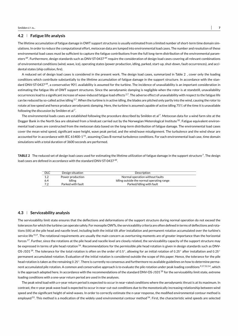
Smilden ET AL. 7
4.2 Fatigue life analysisThe lifetime accumulation of fatigue damage inOWT support structures is usually estimated from a limited number of short-term time domain sim-ulations. In order to reduce the computational effort, metocean data are lumped into environmental load cases. The number and resolution of theseenvironmental load cases must be sufficient to capture the fatigue contributions from the full long-term distribution of the environmental param-eters 49. Furthermore, design standards such as DNV-ST-0437 49 require the consideration of design load cases covering all relevant combinationsof environmental conditions (wind, wave, ice), operating states (power production, idling, parked, start-up, shut-down, fault occurrences), and acci-dental states (ship collision, fire).A reduced set of design load cases is considered in the present work. The design load cases, summarized in Table 2 , cover only the loading
conditions which contribute substantially to the lifetime accumulation of fatigue damage in the support structure. In accordance with the stan-dard DNV-ST-0437 49, a conservative 90% availability is assumed for the turbine. The incidence of unavailability is an important consideration inestimating the fatigue life of OWT support structures. Since the aerodynamic damping is negligible when the rotor is at standstill, unavailabilityoccurrences lead to a significant increase ofwave-induced fatigue load effects 2,7. The adverse effect of unavailabilitywith respect to the fatigue lifecan be reduced by so-called active idling 2,7.When the turbine is in active idling, the blades are pitched only partly into thewind, causing the rotor torotate at low speed and hence produce aerodynamic damping. Here, the turbine is assumed capable of active idling 75% of the time it is unavailablefollowing the discussion by Smilden et al 7.The environmental loads cases are established following the procedure described by Smilden et al 7. Metocean data for a wind farm site at the
Dogger Bank in the North Sea are obtained from a hindcast carried out by the Norwegian Meterological Institute 50. Fatigue equivalent environ-mental load cases are constructed from the metocean data based on the long-term distribution of fatigue damage. The environmental load casescover the mean wind speed, significant wave height, wave peak period, and the wind/wave misalignment. The turbulence and the wind shear areaccounted for in accordance with IEC 61400-1 51, assuming Class B normal turbulence conditions. For each environmental load case, time domainsimulations with a total duration of 3600 seconds are performed.
TABLE 2 The reduced set of design load cases used for estimating the lifetime utilization of fatigue damage in the support structure 7. The designload cases are defined in accordance with the standard DNV-ST-0437 49.
DLC Design situation Description1.2 Power production Normal operation without faults6.4 Idling Idling outside the normal operating range7.2 Parkedwith fault Parked/Idling with fault
4.3 Serviceability analysisThe serviceability limit state ensures that the deflections and deformations of the support structure during normal operation do not exceed thetolerances forwhich the turbine canoperate safely. FormonopileOWTs, the serviceability criteria areoftendefined in termsof deflections and rota-tions (tilt) at the pile head and nacelle level, including both the initial tilt after installation and permanent rotation accumulated over the turbine’sservice life 9,17. The rotational requirements are usually the main concern as overturning moments are of greater importance than the horizontalforces 17. Further, since the rotations at the pile head and nacelle level are closely related, the serviceability capacity of the support structure maybe expressed in terms of pile head rotation 16. Recommendations for the permissible pile head rotation is given in design standards such as DNV-OS-J101 39. The tolerance for the total rotation is often on the order of 0.5◦, allowing for an initial rotation of 0.25◦ after installation and 0.25◦
permanent accumulated rotation. Evaluation of the initial rotation is considered outside the scope of this paper. Hence, the tolerance for the pilehead rotation is taken as the remaining 0.25◦. There is currently no consensus and furthermore no available guidelines on how to determine perma-nent accumulated pile rotation. A common and conservative approach is to evaluate the pile rotation under peak loading conditions 9,17,52,14, whichis the approach adopted here. In accordance with the recommendations of the standard DNV-OS-J101 39 for the serviceability limit state, extremeloading conditions with a one-year return period are used in the analyses.The peakwind loadwith a n-year return period is expected to occur in near-rated conditions where the aerodynamic thrust is at its maximum. In
contrast, the n-year peak wave load is expected to occur in near-cut-out conditions due to themonotonically increasing relationship betweenwindspeed and the significant height of wind-waves. In order to correctly estimate the n-year response, the modified environmental contour method isemployed 53. This method is a modication of the widely used environmental contour method 54. First, the characteristic wind speeds are selected

8 Smilden ET AL.
deterministically as the wind speeds for which the peak wind and wave loads are expected to occur. Then, for each characteristic wind speed, then-year sea state contour is constructed using Rosenblatt’s transformation. In the statistical model, the significant wave height Hs is modeled asdependent on the mean wind speed V while the wave zero-crossing period Tz is modeled as dependent on Hs. In accordance with the standardDNV-ST-0437 49, a three-parameterWeibull distribution is assumed forHs. Further, the conditional distribution ofTz givenHs is assumed to be log-normal 55.The environmental load cases used for estimating the serviceability utilization of the support structure are presented in Table 3 . The environ-
mental load cases cover themeanwind speed, significantwave height, and thewave zero-crossing period. Turbulence andwind shear are accountedfor in accordance with IEC 61400-1 51, assuming Class B normal turbulence conditions. Several combinations of environmental parameters shouldin principle be considered for each loading condition. However, one set of environmental parameters is found sufficient for the analyses performedhere. As both wind and wave are random processes, the maximal pile head rotation is a stochastic variable. In order to estimate the serviceabilityutilization, the maximum pile head rotation must be determined from time series of responses. The expected maximum value of ten one-hour timeseries is taken as themaximum pile head rotation.
TABLE3 The reduced set of environmental load cases used for estimating the serviceability utilization of the support structure. The environmentalload cases cover themeanwind speedV, significant wave heightHs, and wave zero-crossing periodTz.
Envionmental parametersLoading condition V [m/s] Hs [m] Tz [s]One-year peak loading in rated conditions 11.0 4.3 7.0One-year peak loading in cut-out conditions 25.0 7.6 9.7
5 SELECTINGCHARACTERISTIC SOIL PROPERTIESAnalysis of the two-stage controls adaptation requires selecting characteristic soil properties for use in the pre-installation prediction of the struc-tural safetymargins.While several researchers have studied the effects of soil-structure uncertainty in a structural reliability context 56,8,10,12, thereare few publications that deal with the selection of characteristic soil properties 52. In general, the appropriate choice of characteristic soil prop-erties depends on the type of support structure and limit state in consideration. According to the standard DNV-OS-J101 39, a tail quantile in soilproperty distribution should be used if the limit state is governed by a small soil volume. Likewise, the soil property’s mean value should be takenas the characteristic value if the limit state is governed by a large soil volume. Furthermore, the characteristic values should be selected as cautiousestimates of the values governing the limit state in consideration. The geotechnical design of monopile OWT foundations involves a rather largevolume of soil. Consequently, the depth dependent characteristic soil property should be a cautious estimate of the mean trend. The characteristicvalue ξK is typically expressed as themeanminus the standard deviationmultiplied with some factor γK
35, such thatξK,i = µi − γKσi, i = 1, 2, . . . , n (9)
whereµi andσi are themeans and standard deviations at the ndepth decrements. The factor γK is selected based on the required level of caution 35.Design standards, such asDNV-RP-C207 57, provide general guidelines on the selection of γK based on the number of observations in the soil layers.These guidelines are appropriate under the assumption of negligible variance in the design-driving soil properties. This is a reasonable assumptionfor piles under axial loading, for which the soil over the entire embedment length contributes to the load carrying capacity 37. As the followinganalysis will show, this is not necessarily the case for laterally loaded piles such asmonopile OWT foundations.Figure 3 presents the distribution of the fundamental fore-aft natural period for different vertical scales of fluctuation. Only the fore-aft period
is presented here since the fore-aft and side-side bending modes have closely spaced periods with similar distributions. Since the natural periodsare bounded from below by those with fixed boundary conditions at the seabed, their distributions are negatively skewed 26,11,10. As expected, thevariance of the natural period depends on the vertical correlation length. Thus, for limit states that are closely correlated with the natural period,neglecting vertical correlation does not yield a consistent level of safety.Figure 4 presents the horizontally averaged soil properties for all outcomes of the natural period above the 95%-quantile and below the 5%-
quantile. The random field realizations associated with natural periods in the tail quantiles deviate from the mean trend. In general, sand providesgreater soil-pile stiffness than clay. The angle of internal friction therefore exhibits larger deviations from its mean value than the undrained shear
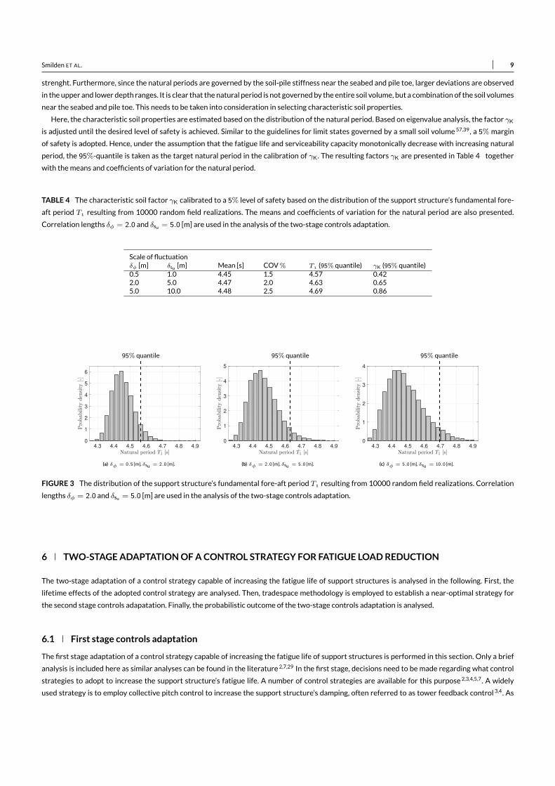
Smilden ET AL. 9strenght. Furthermore, since the natural periods are governed by the soil-pile stiffness near the seabed and pile toe, larger deviations are observedin theupper and lower depth ranges. It is clear that thenatural period is not governedby the entire soil volume, but a combination of the soil volumesnear the seabed and pile toe. This needs to be taken into consideration in selecting characteristic soil properties.Here, the characteristic soil properties are estimated based on the distribution of the natural period. Based on eigenvalue analysis, the factor γK
is adjusted until the desired level of safety is achieved. Similar to the guidelines for limit states governed by a small soil volume 57,39, a 5%marginof safety is adopted. Hence, under the assumption that the fatigue life and serviceability capacity monotonically decrease with increasing naturalperiod, the 95%-quantile is taken as the target natural period in the calibration of γK. The resulting factors γK are presented in Table 4 togetherwith themeans and coefficients of variation for the natural period.
TABLE 4 The characteristic soil factor γK calibrated to a 5% level of safety based on the distribution of the support structure’s fundamental fore-aft period T resulting from 10000 random field realizations. The means and coefficients of variation for the natural period are also presented.Correlation lengths δφ = 2.0 and δsu = 5.0 [m] are used in the analysis of the two-stage controls adaptation.
Scale of fluctuationδφ [m] δsu [m] Mean [s] COV% T (95% quantile) γK (95% quantile)0.5 1.0 4.45 1.5 4.57 0.422.0 5.0 4.47 2.0 4.63 0.655.0 10.0 4.48 2.5 4.69 0.86
4.3 4.4 4.5 4.6 4.7 4.8 4.9
Natural period T1 [s]
0
1
2
3
4
5
6
Probab
ilityden
sity
[-]
95% quantile
(a) δφ = 0.5 [m],δsu = 2.0 [m].
4.3 4.4 4.5 4.6 4.7 4.8 4.9
Natural period T1 [s]
0
1
2
3
4
5
Probab
ilityden
sity
[-]
95% quantile
(b) δφ = 2.0 [m],δsu = 5.0 [m].
4.3 4.4 4.5 4.6 4.7 4.8 4.9
Natural period T1 [s]
0
1
2
3
4
Probab
ilityden
sity
[-]
95% quantile
(c) δφ = 5.0 [m],δsu = 10.0 [m].
FIGURE 3 The distribution of the support structure’s fundamental fore-aft period T resulting from 10000 random field realizations. Correlationlengths δφ = 2.0 and δsu = 5.0 [m] are used in the analysis of the two-stage controls adaptation.
6 TWO-STAGEADAPTATIONOFACONTROL STRATEGY FOR FATIGUE LOADREDUCTIONThe two-stage adaptation of a control strategy capable of increasing the fatigue life of support structures is analysed in the following. First, thelifetime effects of the adopted control strategy are analysed. Then, tradespace methodology is employed to establish a near-optimal strategy forthe second stage controls adapatation. Finally, the probabilistic outcome of the two-stage controls adaptation is analysed.
6.1 First stage controls adaptationThe first stage adaptation of a control strategy capable of increasing the fatigue life of support structures is performed in this section. Only a briefanalysis is included here as similar analyses can be found in the literature 2,7,29 In the first stage, decisions need to be made regarding what controlstrategies to adopt to increase the support structure’s fatigue life. A number of control strategies are available for this purpose 2,3,4,5,7. A widelyused strategy is to employ collective pitch control to increase the support structure’s damping, often referred to as tower feedback control 3,4. As

10 Smilden ET AL.
30 40 50
Friction angle [deg]
-5
-4
-3
-2
-1
50 100 150
Undrained shear strength [kN/m2]
-35
-30
-25
-20
-15
-10
-5
Dep
th[m
] γK = 0γK = ±1
S5%/S95%
(a) δφ = 0.5 [m],δsu = 1.0 [m].
30 40 50
Friction angle [deg]
-5
-4
-3
-2
-1
50 100 150
Undrained shear strength [kN/m2]
-35
-30
-25
-20
-15
-10
-5
Dep
th[m
]
(b) δφ = 2.0 [m],δsu = 5.0 [m].
30 40 50
Friction angle [deg]
-5
-4
-3
-2
-1
50 100 150
Undrained shear strength [kN/m2]
-35
-30
-25
-20
-15
-10
-5
Dep
th[m
]
(c) δφ = 5.0 [m],δsu = 10.0 [m].
FIGURE 4 Horizontally averaged soil properties for all outcomes of the support structure’s fundamental fore-aft period T outside selected tailquantiles in the distrubution of T resulting from 10000 random field realizations. Results are presented for random field realizations resulting innatural periods below the 5%-quantile S% and above the 95%-quantile S%. Correlation lengths δφ = 2.0 and δsu = 5.0 [m] are used in theanalysis of the two-stage controls adaptation.
collective pitch control only effectively reduces loads parallel to the wind direction, it may also be beneficial to increase the damping in the cross-wind direction by either individual pitch control 2, or generator torque control 2,3,5. The effectiveness of the various control strategies depends onthe type of foundation and the site-specific conditions, such as the water depth and the environmental characteristics 2,7.Here, only collective pitch control is adopted to increase the fatigue life of the support structure. Tower feedback control is implemented via an
auxiliary control loop, using the control scheme proposed by Smilden et al. 58. The control scheme extends conventional tower feedback control toprovide both damping and stiffness to the support structure’s fore-aft bending modes. The tower feedback control actions βTFC are governed bythe following control law:
βTFC = − 1
FβA(α)
(KP (x− xref) +KDx
), FβA(α) =
∂FA
∂β
∣∣∣∣∣α
< 0, (10)where KP ≥ 0 is the proportional (stiffness) gain, and KD ≥ 0 is the derivative (damping) gain. The demanded pitch actions are scheduled by thepartial derivative from pitch angle to aerodynamic thrust FβA(α) < 0 where the vector α ∈ R4×1 consists of parameters governing the aerody-namic loads. The reference tower displacement trajectory xref is generated by a referencemodel which estimates thewind-induced progress of thetower displacement. Further, an extended Kalman filter is applied to calculate the required state estimates such as the tower displacement x andthe tower velocity x. The tower feedback controller is operated with different sets of controller gains depending on the operational mode of theturbine. In the partial load region, only derivative action is used, rendering the control scheme a conventional tower feedback controller. In the fullload region, tower feedback control with proportional-derivative action is used.The additional costs of tower feedback control are primarily related to increased wear of various wind turbine components. In particular, it
increases the fatigue loads in the pitch system and drive-train module, including the gearbox assembly 58,7. Hence, the damage equivalent loads inthemain shaft and pitch actuator bearings are taken as parameters to evaluate the effects of tower feedback control 7. The damage equivalent loadsin the main shaft are computed from the time histories of the shaft’s torsional loading with rainflow counting of stress amlitudes. In the case of thepitch actuator bearings, the fatigue damage is governed by the overturningmoments in the actuator and the number of revolutions for the bearing.The load distribution duration method is therefore used to compute the damage equivalent loads in the pitch bearings. For both components, theslope exponent of the S-N curve is taken as 3 in the fatigue calculations 7.Table 5 presents the result of the first stage adaptation of tower feedback control. Tower feedback control significantly increases the fatigue
life of the support structure. Monopile OWT foundations are typically designed for a fatigue life of 50 years 16,17. Moreover, the standard DNV-OS-C101 59 requires a safety factor of at least 3.0 for offshore steel structureswith non-accessible areas. In addition, a corrective factor of 1.4 is appliedto the fatigue damage in order to achieve the target fatigue utilization (D20-year
Max = 1) only if tower feedback control is used. Although there is aslight excess of fatigue life, the dimensions of the foundations are not further optimized. As expected, the fatigue loads in the pitch actuator bear-ings and themain shaft are increased significantly as a result of the additional pitch activity.
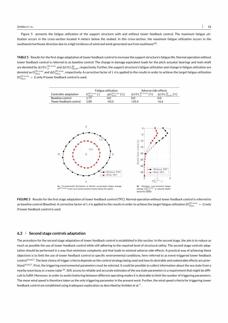
Smilden ET AL. 11Figure 5 presents the fatigue utilization of the support structure with and without tower feedback control. The maximum fatigue uti-
lization occurs in the cross-section located 4 meters below the seabed. In this cross-section, the maximum fatigue utilization occurs in thesouthwest/northeast direction due to a high incidence of wind andwind-generated sea from southwest 60.
TABLE 5 Results for the first stage adaptation of tower feedback control to increase the support structure’s fatigue life. Normal operationwithouttower feedback control is referred to as baseline control. The change in damage equivalent loads for the pitch actuator bearings and main shaftare denoted by∆DEL20-year
β and∆DEL20Shaft, respectively. Further, the support structure’s fatigue utilization and change in fatigue utilization are
denoted asD20-yearMax and∆D20-year
Max , respectively. A corrective factor of 1.4 is applied to the results in order to achieve the target fatigue utilization(D20-year
Max = 1) only if tower feedback control is used.
Fatigue utilization Adverse side-effectsController adaptation D20-year
Max [-] ∆D20-yearMax [%] ∆DEL20-year
β [%] ∆DEL20Shaft [%]Baseline control 1.77 0.0 0.0 0.0
Tower feedback control 1.00 -43.5 +25.4 +6.6
N
E
S
W 0
0.5
1
1.5
Without TFC
With TFC
(a) Circumferential distribution of lifetime accumulated fatigue damageD20-year in the cross-section located 4meters below the seabed.
0 1 2
D20−yearMax [-]
-35
-30
-25
-20
-15
-10
-5
0
Depth
below
seab
ed[m
]
Without TFCWith TFC
(b) Maximum cross-sectional fatiguedamage D
20-yearMax
at selected depthsbelow the seabed.
FIGURE 5 Results for the first stage adaptation of tower feedback control (TFC). Normal operation without tower feedback control is referred toas baseline control (Baseline). A corrective factor of 1.4 is applied to the results in order to achieve the target fatigue utilization (D20-year
Max = 1) onlyif tower feedback control is used.
6.2 Second stage controls adaptationThe procedure for the second stage adaptation of tower feedback control is established in this section. In the second stage, the aim is to reduce asmuch as possible the use of tower feedback control while still adhering to the required level of structural safety. The second stage controls adap-tation should be performed in a way that minimizes complexity and that leads to minimal adverse side-effects. A practical way of achieving theseobjectives is to limit the use of tower feedback control to specific environmental conditions, here referred to as event-triggered tower feedbackcontrol 61,62,7. The best choice of trigger criteria depends on the control strategy being used and how its desirable and undesirable effects are prior-itized 61,62,7. First, the triggering environmental parameters must be selected. It could be possible to collect information about the sea state from anearbywave buoy or awave radar 25. Still, access to reliable and accurate estimates of the sea state parameters is a requirement thatmight be diffi-cult to fulfill. Moreover, in order to avoid chattering between different operatingmodes it is desirable to limit the number of triggering parameters.The mean wind speed is therefore taken as the only triggering parameter in the present work. Further, the wind speed criteria for triggering towerfeedback control are established using tradespace exploration as described by Smilden et al. 7.

12 Smilden ET AL.
It is unnecessary to perform a lifetime fatigue analysis for each combination of trigger criteria. Instead, a post-processing algorithm is applied tocompute the lifetime effects of temporarily enabled tower feedback control 7. First, lifetime fatigue analyses are carried outwith andwithout towerfeedback control. Then, the results from two analyses are merged in combinations corresponding to different trigger criteria. In total, 2048 combi-nations of trigger criteria are possible from the grouping of themetocean data.The tradespaces for event-triggered tower feedback control arepresented inFigure6 . Theeffects of tower feedback control, bothdesirable and
undesirable, are sensitive to the soil conditions. This is expected as themagnitude of the support structure response depends on the global stiffnessand the degree to which the fundamental bending mode is excited. The scenarios with a single trigger criterion are highlighted in the tradespaces.With respect to the pitch actuators, it is optimal to use trigger criteria of the type VTFC ≥ VLim
TFC, meaning that tower feedback control is usedfor wind speeds above VLim
TFC. Notably, the opposite trend is observed for the main shaft, for which trigger criteria of the type VTFC ≤ VLimTFC
are close to optimal. It is clear that the best choice of trigger criteria depends on the priority of the adversely affected components. However, thetradespaces reveal general patterns independent of the site-specific soil conditions.With regard to the second stage controls adaptation it is there-fore reasonable to define a single set of trigger criteria. Here, the pitch actuators are given priority and trigger criteria of the type VTFC ≥ VLim
TFC
are used.
0 5 10 15 20 25 30
∆DEL20−yearβ [%]
-40
-30
-20
-10
0
∆D
20−year
Max
[%]
(a) 99%-quantile.
0 2 4 6
∆DEL20−yearShaft [%]
-40
-30
-20
-10
0
∆D
20−year
Max
[%]
Trade-off scenariosVTFC ≤ V
LimTFC
VTFC ≥ VLimTFC
5
10
15
20
5
10
15
20
VLimTFC
(b) 99%-quantile.
0 5 10 15 20 25 30
∆DEL20−yearβ [%]
-40
-30
-20
-10
0
∆D
20−year
Max
[%]
(c) 1%-quantile.
0 2 4 6
∆DEL20−yearShaft [%]
-40
-30
-20
-10
0
∆D
20−year
Max
[%]
(d) 1%-quantile.
FIGURE 6 Tradespaces used for establishing the procedure for the second stage adaptation of tower feedback control. The tradespaces are con-structed by considering event-triggered tower feedback control with mean wind speed as the triggering parameter. Results are presented forcharacteristic soil properties corresponding to 1% and 99% quantiles in the distribution of the natural period T. The change in damage equivalentloads for the pitch actuator bearings and main shaft are denoted by∆DEL20-year
β and∆DEL20-yearShaft , respectively. Further,∆D20-year
Max denotes thechange in fatigue utilization for the support structure. The stars highlight the scenarios with a single trigger criterion VLim
TFC. Trigger criteria of thetypeVTFC ≥ VLim
TFC (red stars), meaning that tower feedback control is used for wind speeds greater thanVLimTFC, are adopted for the second stage
controls adapatation.
6.3 Probabilistic outcome of the two-stage controls adaptationThe probabilistic outcome of a two-stage adaptation of tower feedback control is analysed in this section.MonteCarlomethodology is employed tocompute the probabilistic outcome of the post-installation adaptation of tower feedback control. First, a set of random field realizations is gener-ated. Then, for each realization, a simple optimization procedure is performed tomaximize the trigger criterionVLim
TFC and therby minimize the use

Smilden ET AL. 13of tower feedback control. The fatigue life criterion is required to be fulfilled only with a certain probability, thus making the optimization problemchance constrained 30. In line with the previous discussion, the margin of safety is taken as approximately 5%. It is computationally impractical toperforma lifetime fatigue analysis for each randomfield realization. Therefore, response surfacemethodology is employed in theMonteCarlo anal-ysis. In order to construct the response surfaces, lifetime fatigue analyses are carried out for selected quantiles in the distribution of the naturalperiod. Furthermore, the analysis considers both a one-to-one and an uncertain relationship between the estimated natural period and the pre-dicted fatigue life of the support structure. The one-to-one correspondence should be interpreted as an idealized situation. In reality, there is stilluncertainty regarding the support structure’s fatigue life when the post-installation controls adaptation is performed.Most of this uncertainty waspresent also in the pre-installation prediction of the fatigue life and need not be accounted for. The use of acceleration data to estimate the naturalperiods introduces uncertainty that was previously not present and should hence be taken into account. The uncertain natural period estimate Tis modeled as normally distributed withmean given by the true natural period T, such that
T1 = T1 + ε, ε ∼ N (0, ησT1) (11)
It is useful to express the post-installation estimation uncertainty as a function of the pre-installation uncertainty in the natural period. The stan-dard deviation of the estimation error ε is therefore given by the standard deviation of the natural period σT multiplied by a factor η.Figure 7 presents the outcomes of the post-installation adaptation of tower feedback control when there is perfect knowledge of the true nat-
ural period (η = 0.0). In the idealized situation, there is approximately a 60% probability of tower feedback control being used (VLimTFC < 26 [m/s])
and a 5% probability of tower feedback control being used to the full extent possible (VLimTFC = 4 [m/s]). Natural periods in between the 40%- and
95%-quantiles lead to varying degree of tower feedback control, and maximum utilization of the support structure’s fatigue life (D20-yearMax = 1.0).
Clearly, as a result of the post-installation controls adaptation, the support structures’ fatigue life is equalized over a range of natural periods. Thisadmits the possibility of decommissioning the turbines accross the wind farm at the same time without wasting structural reserves. In effect, thetwo-stage controls adaptation can also be viewed as ameans of reducing conservatism in the design of the support structures.Figure 8 presents the outcomes of the post-installation adaptation of tower feedback control when there is uncertainty about the true natural
period. As expected, estimation uncertainty lead to an increase in the incidence of tower feedback control. At the present level of uncertainty, thereare instances of tower feedback control across the whole range of natural periods. Nevertheless, the overall degree to which tower feedback con-trol is being used decreases with decreasing natural period. On average, a significant reduction in adverse side-effects is therefore expected evenin the presence of estimation uncertainty. Notably, there are very few instances of tower feedback control not being used at maximum capacity fornatural periods above the 95th-quantile.Table 6 presents the probabilistic outcome of the two-stage adaptation of tower feedback control under varying levels of estimation uncer-
tainty. Furthermore, the average increase in the pitch bearings’ and main shaft’s fatigue loads is presented as a function of the level of estimationuncertainty in Figure 9 . In all cases, the post-installation controls adaptation leads to a significant reduction in the adverse side-effects of towerfeedback control. The proposed methodology adds complexity to the turbines’ control and sensor systems, and to the structural design process ingeneral. A substantial reduction in the adverse side-effects of tower feedback control should be demonstrated in order to justify this added com-plexity. Arguably, even when the estimation uncertainty is on the order of the pre-installation uncertainty in the natural period (η = 1.0), thepost-installation controls adaptation leads to a large reduction in adverse side-effects, particularly for the pitch actuators. Of course, this resultdepends on how the different components are prioritized in the second stage controls adaptation.
TABLE 6 Probabilistic outcome of the two-stage adaptation of tower feedback control. The average change in damage equivalent loads for thepitch actuator bearings and main shaft are denoted as∆DEL20-year
β and∆DEL20-yearShaft , respectively. Further, P[VLim
TFC < 26] is the probability of
tower feedback control being used andP[VLimTFC = 26
] is the probability of it being used to the full extent possible. The probability of themaximumfatigue utilization being exceededP
[D20-year
Max > 1.0] can be interpreted as the probability of failure. The results are generated from10000 random
field realizations.
Case description ∆DEL20-yearβ [%] ∆DEL20-year
Shaft [%] P[VLimTFC = 4
] [%] P[VLimTFC < 26
] [%] P[D20-year
Max > 1.0] [%]
Conventional one-stage adaptation 22.1 6.2 100.0 100.0 5.0Two-stage adaptation η = 0.0 3.0 2.3 5.0 58.4 5.0Two-stage adaptation η = 0.25 5.4 3.3 10.6 76.3 6.2Two-stage adaptation η = 0.5 8.8 4.4 22.0 88.2 6.2Two-stage adaptation η = 0.75 12.2 5.0 36.0 92.7 6.2Two-stage adaptation η = 1.0 15.1 5.4 52.8 94.4 6.2
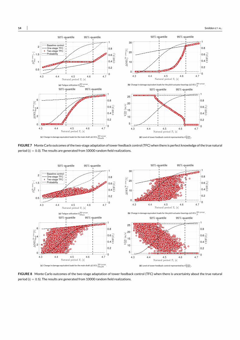
14 Smilden ET AL.
4.3 4.4 4.5 4.6 4.7Natural period T1 [s]
0.5
1
1.5
2
D20−year
Max
[−]
0
0.2
0.4
0.6
0.8
1
CDF(T
1)
Baseline control
One-stage TFC
Two-stage TFC
Probability
95%-quantile50%-quantile
(a) Fatigue utilizationD20-yearMax
.
4.3 4.4 4.5 4.6 4.7
Natural period T1 [s]
0
10
20
30
∆DEL20−year
β[%
]
0
0.2
0.4
0.6
0.8
1
CDF(T
1)
95%-quantile50%-quantile
(b) Change in damage equivalent loads for the pitch actuator bearings∆DEL20-yearβ
.
4.3 4.4 4.5 4.6 4.7
Natural period T1 [s]
0
2
4
6
∆DEL20−year
Shaft
[%]
0
0.2
0.4
0.6
0.8
1
CDF(T
1)
95%-quantile50%-quantile
(c) Change in damage equivalent loads for themain shaft∆DEL20-yearShaft
.
4.3 4.4 4.5 4.6 4.7
Natural period T1 [s]
5
10
15
20
25
VLim
TFC[m
/s]
0
0.2
0.4
0.6
0.8
1
CDF(T
1)
95%-quantile50%-quantile
(d) Level of tower feedback control represented byVLimTFC .
FIGURE7 MonteCarlo outcomes of the two-stage adaptation of tower feedback control (TFC)when there is perfect knowledge of the true naturalperiod (η = 0.0). The results are generated from 10000 random field realizations.
4.3 4.4 4.5 4.6 4.7Natural period T1 [s]
0.5
1
1.5
2
D20−year
Max
[−]
0
0.2
0.4
0.6
0.8
1
CDF(T
1)
Baseline control
One-stage TFC
Two-stage TFC
Probability
95%-quantile50%-quantile
(a) Fatigue utilizationD20-yearMax
.
4.3 4.4 4.5 4.6 4.7
Natural period T1 [s]
0
10
20
30
∆DEL20−year
β[%
]
0
0.2
0.4
0.6
0.8
1
CDF(T
1)
95%-quantile50%-quantile
(b) Change in damage equivalent loads for the pitch actuator bearings∆DEL20-yearβ
.
4.3 4.4 4.5 4.6 4.7
Natural period T1 [s]
0
2
4
6
∆DEL20−year
Shaft
[%]
0
0.2
0.4
0.6
0.8
1
CDF(T
1)
95%-quantile50%-quantile
(c) Change in damage equivalent loads for themain shaft∆DEL20-yearShaft
.
4.3 4.4 4.5 4.6 4.7
Natural period T1 [s]
5
10
15
20
25
VLim
TFC[m
/s]
0
0.2
0.4
0.6
0.8
1
CDF(T
1)
95%-quantile50%-quantile
(d) Level of tower feedback control represented byVLimTFC .
FIGURE 8 Monte Carlo outcomes of the two-stage adaptation of tower feedback control (TFC) when there is uncertainty about the true naturalperiod (η = 0.5). The results are generated from 10000 random field realizations.

Smilden ET AL. 15
0.0 0.25 0.5 0.75 1.0
Estimation uncertainty η
0
5
10
15
20
25
∆DEL20−year
β[%
]
Two-stage tower feedback controlOne-stage tower feedback control
(a)
0.0 0.25 0.5 0.75 1.0
Estimation uncertainty η
0
2
4
6
∆DEL20−year
Shaft
[%]
(b)
FIGURE 9 Probabilistic outcome of the two-stage adaptation of tower feedback control. The average change in damage equivalent loads for thepitch actuator bearings andmain shaft are denoted as∆DEL20-year
β and∆DEL20-yearShaft , respectively. The results are generated from10000 random
field realizations.
7 TWO-STAGEADAPTATIONOFACONTROL STRATEGY FOR SERVICEABILITY LOADREDUCTIONThe two-stage adaptation of a control strategy capable of increasing the serviceability capacity of support structures is analysed in the following.First, the lifetime effects of the adopted control strategy are analysed. Then, the procedure for the second stage controls adapatation is established.Finally, the probabilistic outcome of the two-stage controls adaptation is analysed.
7.1 First stage controls adaptationThe first stage adaptation of a control strategy capable of increasing the serviceability capacity of support structures is performed in this section.Unlike fatigue-reducing controlmeasures, methodology for improving serviceability is notmuch discussed in the literature onwind turbine control.While the support structures’ fatigue life is governed by normal loading conditions, their serviceability capacities are determined by the ability toresist tilting under certain loading conditions. Control measures for improving serviceability can therefore be targetedmore directly at the design-driving loads. Reducing the maximum aerodynamic thrust via so-called peak shaving is effective for reducing wind-induced overturning momentsin near-rated conditions 6,63. Thus, peak shaving provides ameans of increasing the serviceability capacity of support structures.Peak shaving is achieved by pitching to feather to reduce the rotor’s aerodynamic efficiency in near-rated conditions. Implementing such a con-
trol strategy is fairly straightforward and requires only a simple mapping from a selected peak shaving parameter to the rotor’s collective pitchangle 63. In the present work, the power output POut is taken as the peak shaving parameter and the demanded pitch angle βPS is calculated usingthe following relationship:
βPS = max(
min(β(POut;βMax
PS
), βMax
PS
), 0), β
(POut;βMax
PS
)= a(βMaxPS
)POut + b
(βMaxPS
) (12)The level of peak shaving depends on the prescribed pitch angle βMax
PS at which rated power is reached. Within the peak shaving region, the pitchangle is adjusted as a linear function of the power output. For a given level of peak shaving, the constants a and b are selected with the aim of mini-mizing adverse side-effects. A more favourable trade-off between load reduction and adverse side-effects can be achieved by using a higher orderpeak shaving method, such as those described by Perley et al 63. However, given the relatively low potential for improvement, further optimizationefforts are considered outside the scope of this paper.Since peak shaving is achieved by reducing the rotor’s aerodynamic efficiency, it unavoidably leads to power losses that may significantly reduce
the lifetime energy yield. Support structures are typically reported to contribute approximately 20% to the cost of offshore wind energy 2,61. Thus,any percentage loss of power production revenue must be offset by a five-fold percentage reduction in the cost of support structures. The lifetimeenergy yield is estimated from time histories of power output obtained from aero-hydro-servo-elastic simulations. First, themeanwind speed datais grouped into intervals of 1 [m/s]. Then, for each interval, simulations of 3600 [s] duration are performed, taking themidpoint of the interval as themeanwind speed. Turbulence andwind shear are accounted for in accordancewith IEC61400-1 51, assumingClass B normal turbulence conditions.The negligible effect of wave loads on the power output is not accounted for in the analysis.Table 7 presents the result of the first stage adaptation of peak shaving. The selected level of peak shaving leads to a significant increase in the
serviceability capacity. No strategies have been adopted to increase the serviceability capacity in near-cut-out conditions. The near-cut-out ser-viceability capacity is therefore taken as the target capacity in near-rated conditions. Furthermore, a corrective factor is applied to the results inorder to achieve the target serviceability utilization (θ1-yearMax = 1) only if peak shaving is used. As expected, peak shaving reduces the lifetime energyyield. At the present level of peak shaving (βMax
PS = 6◦), the cost savings enabled by increasing the serviceability capacity are unlikely to offset the

16 Smilden ET AL.
loss of power production revenue.Figure10 presents theeffect of the appliedpeak shaving strategyon selectedwind turbineparameters as a functionofwind speed. It is apparent
that peak shaving reduces themaximum steady-state thrust at the expense of power losses. Although these power losses are limited to a relativelysmall range of wind speeds, they occur in wind conditions which contribute significantly to the lifetime energy yield. Their effect in terms of lostpower production is therefore considerable.
TABLE 7 Results for the first stage adaptation of peak shaving to increase the support structure’s serviceability capacity. Normal operation with-out peak shaving is referred to as baseline control. The near-rated and near-cut-out serviceability utilization are denoted as θ1-yearRated and θ1-yearCut-out,respectively. Further, the change inmaximum serviceability utilization and power production are denoted by∆θ1-yearMax and∆P20-year
Out , respectively.A corrective factor of 0.49 is applied to the results in order to achieve the target serviceability utilization (θ20-yearMax = 1) only if peak shaving is used.
Serviceability utilization Adverse side-effectsController adaptation θ1-yearRated [-] θ1-yearCut-out [-] ∆θ1-yearMax [%] ∆P20-year
Out [%]Baseline control 1.6 1.0 0.0 0.0Peak shaving 1.0 1.0 -37.4 -2.1
6 8 10 12 14 16
Wind speed [m/s]
0.5
1
1.5
Aerodynam
icthrust
[MN]
0
2
4
6
8
10
12
Pow
erou
tput[M
W]
Pitch
angle[deg]
Thrust w/ PSThrust w/o PSPower w/ PSPower w/o PSPitch w/ PSPitch w/o PS
VR(βMaxPS )
(a) Selected wind turbine parameters as a function of wind speed.
5 10 15 20 25
Wind speed [m/s]
0
2
4
6
8
10
12
Meanpow
erou
tput[M
W]
0
5
10
15
Probab
ility[%
]
Power w/o PSPower with PSProbability
(b) Non-weightedmean power output as a function of wind speed.
FIGURE 10 The effect of the applied peak shaving (PS) strategy on selected wind turbine parameters as a function of wind speed. The wind speedat which rated power is reachedVR(βMax
PS )with the applied level of peak shaving (βMaxPS = 6◦) is indicated.
7.2 Second stage controls adaptationThe procedure for the second stage adaptation of peak shaving is established in the following. For a given outcome of the site-specific soil condi-tions, the required level of serviceability load reduction can be achieved by straightforward adjustment of βMax
PS . The result is, of course, a trade-offbetween serviceability load reduction and power production.The trade-off between reduction of serviceability utilization in rated conditions and lifetime energy yield is presented in Figure 11 . Increasing
the peak shaving yields diminishing returns in terms of serviceability utilization. There is clearly a threshold beyond which increasing the service-ability capacity cannot justify the added power losses. Like tower feedback control, peak shaving ismost effectivewhen the soil-pile stiffness is low.Due to the nonlinear behaviour of the soil, reducing the overturning moment has a greater effect on the tilt angle when the soil undergoes largedeformations. Accordingly, the difference between the serviceability utilization in cut-out and rated conditions without peak shaving decreases asa function of soil-pile stiffness. Notably, the cost of increasing the near-rated serviceability capacity to eliminate this difference appears not to bevery sensitive to variations the soil conditions. It is therefore reasonable to apply the samemaximum level of peak shaving (βMax
PS = 6◦) in the firstand second stage controls adaptation.

Smilden ET AL. 17
-8 -6 -4 -2 0
∆P20−yearOut [%]
-50
-40
-30
-20
-10
0
∆θ1−year
Rated[%
]
0
2
4
6
8
10
βMaxPS
θ1-yearCut-out
(a) 1%-quantile.
-8 -6 -4 -2 0
∆P20−yearOut [%]
-50
-40
-30
-20
-10
0
∆θ1−year
Rated[%
]
θ1-yearCut-out
(b) 99%-quantile.
FIGURE11 Trade-off between reduction of serviceability utilization in rated conditions∆θ1-yearRated and power production change∆P20-yearOut . Results
are presented for characteristic soil properties corresponding to 1%- and 99%-quantiles in the distribution of the natural period T.
7.3 Probabilistic outcome of the two-stage controls adaptationThe probabilistic outcome of the two-stage adaptation of peak shaving is analysed in this section. The procedure for calculating the probabilisticoutcomeof thepost-installationadaptationof peak shaving is similar to thatof tower feedback control. First, a set of randomfield realizations is gen-erated. Then, for each realization, an optimization procedure is performed to minimize the level of peak shaving and thereby the associated powerlosses. Response surfaces are constructed by carrying out serviceability analyses under different levels of peak shaving for selected quantiles in thedistribution of the natural period. Uncertainty in the estimates of the natural period is modeled following the approach proposed in Section 6.3.The outcomes of the post-installation adaptation of peak shaving when there is perfect knowledge of the true natural period is presented in
Figure 12 . As expected, maximum peak shaving (βPSMax = 6◦) is employed only if the natural period is at or above its 95%-quantile. Furthermore,
the natural period below which peak shaving is not used at all (βPSMax = 0◦) falls at approximately the 70%-quantile. Instances of natural periods
in between these quantiles lead to varying degree of of peak shaving, and maximum utilization of the support structure’s serviceability capacity(θ1-yearMax = 1.0).Figure 13 presents the outcomes of the post-installation adaptation of peak shaving when there is uncertainty about the true natural period.
Except for a few instances, maximum peak shaving is employed consistently for natural periods above the 95%-quantile. At the present level ofuncertainty, the natural period below which there are no instances of peak shaving is reduced to approximately the 5%-quantile. Hence, the totalincidence of peak shaving and its associated power losses is significantly increased comparedwith the idealized situationwithout estimation uncer-tainty.Table 8 presents the probabilistic outcome of the two-stage adaptation of peak shaving under varying levels of estimation uncertainty. Further-
more, themean change in the lifetime energy yield is presented as a function of the level of uncertainty in Figure 14 . The post-installation controlsadaptation leads to a substantial reduction of the average power production losses. As expected, the incidence of peak shaving and themean changein the lifetime energy yield increaseswith increasing estimation uncertainty. Although the average power losses are reduced, theymight still be toolarge to be offset by the cost savings enabled by peak shaving. Nevertheless, the results highlight an important implication of the proposedmethod-ology. Since the adverse side-effects on average is reduced by up to an order of magnitude, a post-installation adaptation of load reducing controlscould enable the use of control strategies that were previously not economically viable. At least, it would enable using control strategies to a fullerextent of their capabilities.
8 CONCLUSIONSIn this paper, the potential of making turbine-specific adjustments to the wind turbines’ control systems after their installation was analysed. Theanalysis considered the structural design of a 10MWmonopile offshore wind turbine under uncertainties in the geotechnical properties. An adap-tation of the wind turbines’ control system in two stages was proposed. In the first stage, carried out during the structural design process, controlstrategies were adopted to reduce the support structure’s load effects. In this stage, the structural capacities were uncertain due to inherent vari-ability in the site-specific soil properties. Under the assumption that the true structural capacities could be estimated once the turbines wereinstalled, the second stage controls adaptation was carried out. The objective of the second stage was to minimize the use of the control strategiesadopted in the first stage, while still adhering to the required level of structural safety. Two control strategieswere considered in separate analyses.In both analyses, the two-stage controls adaptation was analysed using response surfacemethodology andMonte Carlo simulations. The response
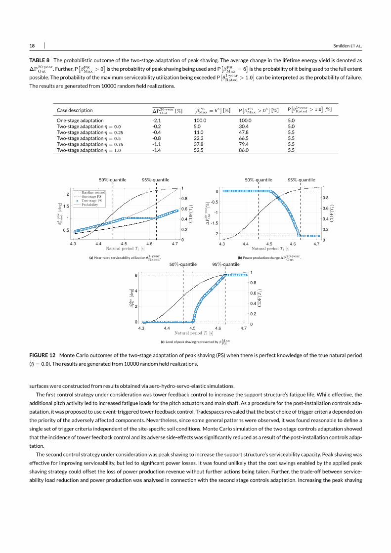
18 Smilden ET AL.
TABLE 8 The probabilistic outcome of the two-stage adaptation of peak shaving. The average change in the lifetime energy yield is denoted as∆P20-year
Out . Further,P[βPSMax > 0
] is the probability of peak shaving being used andP[βPSMax = 6
] is the probability of it being used to the full extentpossible. The probability of themaximum serviceability utilization being exceededP
[θ1-yearRated > 1.0
] can be interpreted as the probability of failure.The results are generated from 10000 random field realizations.
Case description ∆P20-yearOut [%] [
βPSMax = 6◦] [%] P
[βPSMax > 0◦] [%] P
[θ1-yearRated > 1.0
] [%]One-stage adaptation -2.1 100.0 100.0 5.0Two-stage adaptation η = 0.0 -0.2 5.0 30.4 5.0Two-stage adaptation η = 0.25 -0.4 11.0 47.8 5.5Two-stage adaptation η = 0.5 -0.8 22.3 66.5 5.5Two-stage adaptation η = 0.75 -1.1 37.8 79.4 5.5Two-stage adaptation η = 1.0 -1.4 52.5 86.0 5.5
4.3 4.4 4.5 4.6 4.7
Natural period T1 [s]
0.5
1
1.5
2
θ1−
year
Rated
[deg]
0
0.2
0.4
0.6
0.8
1CDF(T
1)
Baseline controlOne-stage PSTwo-stage PSProbability
95%-quantile50%-quantile
(a) Near-rated serviceability utilizationθ1-yearRated
.
4.3 4.4 4.5 4.6 4.7
Natural period T1 [s]
-2
-1.5
-1
-0.5
0
∆P20−year
Out
[%]
0
0.2
0.4
0.6
0.8
1
CDF(T
1)
95%-quantile50%-quantile
(b) Power production change∆P20-yearOut
.
4.3 4.4 4.5 4.6 4.7
Natural period T1 [s]
0
2
4
6
βMax
PS
[deg]
0
0.2
0.4
0.6
0.8
1
CDF(T
1)
95%-quantile50%-quantile
(c) Level of peak shaving represented byβMaxPS
FIGURE 12 Monte Carlo outcomes of the two-stage adaptation of peak shaving (PS) when there is perfect knowledge of the true natural period(η = 0.0). The results are generated from 10000 random field realizations.
surfaces were constructed from results obtained via aero-hydro-servo-elastic simulations.The first control strategy under consideration was tower feedback control to increase the support structure’s fatigue life. While effective, the
additional pitch activity led to increased fatigue loads for the pitch actuators and main shaft. As a procedure for the post-installation controls ada-patation, it was proposed to use event-triggered tower feedback control. Tradespaces revealed that the best choice of trigger criteria depended onthe priority of the adversely affected components. Nevertheless, since some general patterns were observed, it was found reasonable to define asingle set of trigger criteria independent of the site-specific soil conditions. Monte Carlo simulation of the two-stage controls adaptation showedthat the incidence of tower feedback control and its adverse side-effectswas significantly reduced as a result of the post-installation controls adap-tation.The second control strategy under consideration was peak shaving to increase the support structure’s serviceability capacity. Peak shaving was
effective for improving serviceability, but led to significant power losses. It was found unlikely that the cost savings enabled by the applied peakshaving strategy could offset the loss of power production revenue without further actions being taken. Further, the trade-off between service-ability load reduction and power production was analysed in connection with the second stage controls adaptation. Increasing the peak shaving

Smilden ET AL. 19
4.3 4.4 4.5 4.6 4.7
Natural period T1 [s]
0.5
1
1.5
2
θ1−
year
Rated
[deg]
0
0.2
0.4
0.6
0.8
1
CDF(T
1)
Baseline controlOne-stage PSTwo-stage PSProbability
95%-quantile50%-quantile
(a) Near-rated serviceability utilizationθ1-yearRated
.
4.3 4.4 4.5 4.6 4.7
Natural period T1 [s]
-2
-1.5
-1
-0.5
0
∆P20−year
Out
[%]
0
0.2
0.4
0.6
0.8
1
CDF(T
1)
95%-quantile50%-quantile
(b) Power production change∆P20-yearOut
.
4.3 4.4 4.5 4.6 4.7
Natural period T1 [s]
0
2
4
6
βMax
PS
[deg]
0
0.2
0.4
0.6
0.8
1
CDF(T
1)
95%-quantile50%-quantile
(c) Level of peak shaving represented byβMaxPS .
FIGURE 13 Monte Carlo outcomes of the two-stage adaptation of peak shaving (PS) when there is uncertainty about the true natural period(η = 0.5). The results are generated from 10000 random field realizations.
0.0 0.25 0.5 0.75 1.0
Estimation uncertainty η
-2
-1.5
-1
-0.5
0
∆P20−year
Out
[%]
Two-stage peak shavingOne-stage peak shaving
FIGURE 14 Probabilistic outcome of the two-stage adaptation of tower feedback control. The average change in power production is denoted as∆P20-year
Out . The results are generated from 10000 random field realizations.
was found to yield diminishing returns in terms of serviceability utilization. As expected, Monte Carlo simulation showed that the post-installationcontrols adaptation led to a significant reduction in the incidence of peak shaving and its associated power losses.
ACKNOWLEDGMENTSThis work has been carried out at the Centre for AutonomousMarineOperations and Systems (NTNUAMOS). TheNorwegian Research Council isacknowledgedas themain sponsor ofNTNUAMOS. Thisworkwas supportedby theResearchCouncil ofNorway through theCentres of Excellencefunding scheme, Project number 223254 - NTNUAMOS.
References1. HoA,MbistrovaA, CorbettaG, Pineda I, RubyK. TheEuropean offshorewind industry-key trends and statistics.Report. Brussels: EuropeanWindEnergy Association. 2016;.
20 Smilden ET AL.
2. Fischer Tim Andreas.Mitigation of aerodynamic and hydrodynamic induced loads of offshore wind turbines. Shaker; 2012. University of Stuttgart.3. Hooft EL, Schaak P, Van Engelen TG.Wind turbine control algorithms.DOWEC project-DOWEC-F1W1-EH-03-094/0, Task-3 report. 2003;.4. Bossanyi EA.Wind turbine control for load reduction.Wind energy. 2003;6(3):229–244.5. Bossanyi EA, Ramtharan G, Savini B. The importance of control in wind turbine design and loading. In: :1269–1274IEEE; 2009.6. Fischer Boris, Shan Martin. A Survey on Control mMethods for the Mitigation of Tower Loads. Fraunhofer-Institute for Wind Energy and EnergySystems Technology, IWES Project report 01/104256. 2013;.
7. Smilden Emil, Bachynski Erin E., Sørensen Asgeir J., Amdahl Jørgen. Site-specific contoller design for monopile offshore wind turbines.MarineStructures. 2018;.
8. Carswell Wystan, Arwade Sanjay Raja, DeGroot Don J, Lackner Matthew A. Soil–structure reliability of offshore wind turbine monopilefoundations.Wind energy. 2015;18(3):483–498.
9. CarswellW,Arwade SR,DeGrootDJ,MyersAT.Natural frequency degradation andpermanent accumulated rotation for offshorewind turbinemonopiles in clay. Renewable Energy. 2016;97:319–330.
10. Andersen Lars Vabbersgaard, Vahdatirad MJ, Sichani Mahdi Teimouri, Sørensen John Dalsgaard. Natural frequencies of wind turbines onmonopile foundations in clayey soilsâATA probabilistic approach. Computers and Geotechnics. 2012;43:1–11.
11. Damgaard Mads, Bayat Mehdi, Andersen Lars Vabbersgaard, Ibsen Lars Bo. Assessment of the dynamic behaviour of saturated soil subjectedto cyclic loading from offshoremonopile wind turbine foundations. Computers and Geotechnics. 2014;61:116–126.
12. DamgaardMads, Andersen Lars Vabbersgaard, Ibsen Lars Bo, Toft Henrik Stensgaard, Sørensen JohnDalsgaard. A probabilistic analysis of thedynamic response of monopile foundations: Soil variability and its consequences. Probabilistic EngineeringMechanics. 2015;41:46–59.
13. Lombardi Domenico, Bhattacharya Subhamoy, Wood David Muir. Dynamic soil–structure interaction of monopile supported wind turbines incohesive soil. Soil Dynamics and Earthquake Engineering. 2013;49:165–180.
14. Bhattacharya Subhamoy. Challenges in design of foundations for offshore wind turbines. Engineering & Technology Reference. 2014;1(1):922.15. Arany László, Bhattacharya Subhamoy, Macdonald John, Hogan S John. Simplified critical mudline bending moment spectra of offshore wind
turbine support structures.Wind Energy. 2015;18(12):2171–2197.16. Arany Laszlo, Bhattacharya Subhamoy, Macdonald John, Hogan SJ. Design of monopiles for offshore wind turbines in 10 steps. Soil Dynamics
and Earthquake Engineering. 2017;92:126–152.17. Arany László, Bhattacharya Subhamoy, Macdonald John HG, Hogan S John, others . A critical review of serviceability limit state requirements
for monopile foundations of offshore wind turbines. In: Offshore Technology Conference; 2015.18. Seidel Marc, Voormeeren Sven, Steen Jan-Bart. State-of-the-art design processes for offshore wind turbine support structures. Stahlbau.
2016;85(9):583–590.19. Martinez-LuengoMaria, Kolios Athanasios,Wang Lin. Structural health monitoring of offshore wind turbines: A review through the Statistical
Pattern Recognition Paradigm. Renewable and Sustainable Energy Reviews. 2016;64:91–105.20. Gomez Hugo C, Gur Turel, Dolan Dan. Structural condition assessment of offshore wind turbine monopile foundations using vibration
monitoring data. In: :86940BInternational Society for Optics and Photonics; 2013.21. Smarsly Kay, Hartmann Dietrich, Law Kincho H. A computational framework for life-cycle management of wind turbines incorporating
structural healthmonitoring. Structural HealthMonitoring. 2013;12(4):359–376.22. Devriendt Christof, Guillaume Patrick. Identification of modal parameters from transmissibility measurements. Journal of Sound and Vibration.
2008;314(1-2):343–356.23. Devriendt Christof, Jordaens Pieter Jan, De Sitter Gert, Guillaume Patrick. Damping estimation of an offshore wind turbine on a monopile
foundation. IET Renewable Power Generation. 2013;7(4):401–412.

Smilden ET AL. 21
24. Devriendt Christof, Magalhães Filipe, Weijtjens Wout, De Sitter Gert, Cunha Álvaro, Guillaume Patrick. Structural health monitoring ofoffshore wind turbines using automated operational modal analysis. Structural HealthMonitoring. 2014;13(6):644–659.
25. Weijtjens Wout, Verbelen Tim, De Sitter Gert, Devriendt Christof. Foundation structural health monitoring of an offshore wind turbineâATafull-scale case study. Structural HealthMonitoring. 2016;15(4):389–402.
26. Damgaard Mads, Ibsen Lars Bo, Andersen Lars Vabbersgaard, Andersen Jacob KF. Cross-wind modal properties of offshore wind turbinesidentified by full scale testing. Journal ofWind Engineering and Industrial Aerodynamics. 2013;116:94–108.
27. Hansen Morten Hartvig, Thomsen Kenneth, Fuglsang Peter, Knudsen T. Two methods for estimating aeroelastic damping of operational windturbinemodes from experiments.Wind Energy. 2006;9(1-2):179–191.
28. SeidelMarc. Design of support structures for offshorewind turbines–Interfaces between project owner, turbinemanufacturer, authorities anddesigner. Stahlbau. 2010;79(9):631–636.
29. Fischer T, Vries W, Rainey P, Schmidt B, Argyriadis K, Kühn M. Offshore support structure optimization by means of integrated design andcontrols.Wind Energy. 2012;15(1):99–117.
30. King Alan J,Wallace SteinW.Modeling with stochastic programming. Springer Science & BusinessMedia; 2012.31. IEC 61400-3 .Wind Turbines–Part 3: Design Requirements for OffshoreWind Turbines.Design standard. 2009;.32. Phoon Kok-Kwang, Kulhawy FredH. Characterization of geotechnical variability. Canadian Geotechnical Journal. 1999;36(4):612–624.33. Phoon Kok-Kwang, Kulhawy FredH. Evaluation of geotechnical property variability. Canadian Geotechnical Journal. 1999;36(4):625–639.34. Vanmarcke Erik H. Probabilistic modeling of soil profiles. Journal of the geotechnical engineering division. 1977;103(11):1227–1246.35. Schneider Hans R, Schneider Mark A. Dealing with uncertainties in EC7 with emphasis on determination of characteristic soil properties.
Modern Geotechnical Design Codes of Practice (Arnold P, Fenton GA, Hicks MA and Schweckendiek T (eds)). IOS Press, Rotterdam, the Netherlands.2012;:87–101.
36. Prendergast LJ, Reale C, Gavin K. Probabilistic examination of the change in eigenfrequencies of an offshore wind turbine under progressivescour incorporating soil spatial variability.Marine Structures. 2018;57:87–104.
37. Ronold Knut O. Characteristic soil strength for axial pile capacity and its estimationwith confidence for offshore applications. Structural Safety.2016;63:81–89.
38. API, RP . 2GEO (2011). Recommended Practice for Geotechnical Foundation Design Consideration. 2011;.39. DNVDet Norske Veritas. DNV-OS-J101Offshore Standard: Design of OffshoreWind Turbine Structures.DNV AS, Høvik, Norway. 2014;.40. Murchison JackM, O’Neill MichaelW. Evaluation of py relationships in cohesionless soils. In: :174–191ASCE; 1984.41. Matlock Hudson. Correlations for design of laterally loaded piles in soft clay.Offshore technology in civil engineeringâAŹs hall of fame papers from
the early years. 1970;:77–94.42. Reese Lymon C, Welch Robert C. Lateral loading of deep foundations in stiff clay. Journal of Geotechnical and Geoenvironmental Engineering.
1975;101(ASCE# 11456 Proceeding).43. Bak C, Zahle F, Bitsche R, et al. Description of the DTU 10MWreference wind turbine.DTUWind Energy Report-I-0092. 2013;.44. HansenMorten Hartvig, Henriksen Lars Christian. Basic DTUwind energy controller. : DTUWind Energy; 2013.45. Bachynski Erin E, Ormberg Harald. Hydrodynamic Modeling of Large-Diameter Bottom-Fixed Offshore Wind Turbines. In:
:V009T09A051American Society ofMechanical Engineers; 2015.46. Ormberg Harald, Bachynski Erin E, others . Global analysis of floating wind turbines: Code development, model sensitivity and benchmark
study. In: International Society of Offshore and Polar Engineers; 2012.47. DNVGL . DNV-RP-C205. Environmental conditions and environmental loads. 2010;.
22 Smilden ET AL.
48. Jonkman Bonnie J. TurbSim user’s guide. 2009;.49. GL DNV. DNVGL-ST-0437: Loads and site conditions for offshore wind turbines.DNVGL, Høvik, Norway. 2016;.50. Reistad Magnar, Breivik Øyvind, Haakenstad Hilde, Aarnes Ole Johan, Furevik Birgitte R, Bidlot Jean-Raymond. A high-resolution hindcast of
wind andwaves for the North Sea, the Norwegian Sea, and the Barents Sea. Journal of Geophysical Research: Oceans. 2011;116(C5).51. International Electrotechnical Commission (IEC) . IEC 61400-1:Wind turbines part 1: Design requirements. : ; 2005.52. Andersen Lars Vabbersgaard, Sørensen John Dalsgaard, Kim Sun-Bin, et al. Influence of Characteristic-Soil-Property-Estimation Approach on
the Response ofMonopiles for OffshoreWind Turbines. Journal of Ocean andWind Energy. 2015;2(3):160–167.53. Li Qinyuan, Gao Zhen, Moan Torgeir. Modified environmental contour method for predicting long-term extreme responses of bottom-fixed
offshore wind turbines.Marine Structures. 2016;48:15–32.54. Winterstein Steven R, Ude Todd C, Cornell C Allin, Bjerager Peter, Haver Sverre. Environmental parameters for extreme response: Inverse
FORMwith omission factors. Proceedings of the ICOSSAR-93, Innsbruck, Austria. 1993;:551–557.55. Johannessen Kenneth, Meling Trond Stokka, Hayer Sverre, others . Joint distribution for wind and waves in the northern north sea. In:
International Society of Offshore and Polar Engineers; 2001.56. MuskulusM, Schafhirt S. Reliability-based design of wind turbine support structures. In: ; 2015.57. GL DNV. Statistical representation of soil data.DNV-RP-C207. 2012;.58. Smilden Emil, Bachynski Erin E., Sørensen Asgeir J., Amdahl Jørgen.Wave Distrurbance Rejection forMonopile OffshoreWind Turbines.Wind
Energy. 2018;.59. DNVGL . OS-C101.Design of Offshore Steel Structures. 2011;.60. Horn Jan-Tore, Bitner-Gregersen Elzbieta, Krokstad Jørgen R, Leira Bernt J, Amdahl Jørgen. A new combination of conditional environmental
distributions. Applied Ocean Research. 2018;73:17–26.61. Shrestha Binita, Kühn Martin. Tailoring the Employment of Offshore Wind Turbine Support Structure Load Mitigation Controllers. In:
:052032IOP Publishing; 2016.62. Shrestha Binita, Kühn Martin. Adaptation of Controller Concepts for Support Structure Load Mitigation of Offshore Wind Turbines. Energy
Procedia. 2016;94:241–248.63. Perley Thomas Franklin, Busbey Bruce Clark, Gerber Brandon Shane. System and methods for determining pitch angles for a wind turbine during
peak shaving. US Patent App. 13/359,837; 2013.
How to cite this article: E. Smilden, S. Sørum, E. Bachynski, A. Sørensen, and J. Amdahl (2016), Post-installation adaptation of offshorewind turbinecontrols, Journal ofWind Energy, 2018;00:1–22.