structural diagnosis implementation of dymola models...

Master of Science Thesis in Electrical EngineeringDepartment of Electrical Engineering, Linköping University, 2017

Structural DiagnosisImplementation of DymolaModels using Matlab FaultDiagnosis Toolbox

Petter Lannerhed

Master of Science Thesis in Electrical Engineering

Structural Diagnosis Implementation of Dymola Models using Matlab FaultDiagnosis Toolbox

Petter Lannerhed

LiTH-ISY-EX--17/5031--SE

Supervisor: PhD student Viktor Leekisy, Linköpings universitet

PhD Ylva NilssonAeronotics, Saab

Examiner: PhDMattias Krysanderisy, Linköpings universitet

Division of Vehicular SystemsDepartment of Electrical Engineering

Linköping UniversitySE-581 83 Linköping, Sweden

Copyright © 2017 Petter Lannerhed

For most diagnosis all that is needed is an ounce of knowledge, an ounce ofintelligence, and a pound of thoroughness.

- John Murtagh

Abstract

Models are of great interest in many fields of engineering as they enable predic-tion of a systems behaviour, given an initial mode of the system. However, in thefield of model-based diagnosis the models are used in a reverse manner, as theyare combined with the observations of the systems behaviour in order to estimatethe system mode. This thesis describes computation of diagnostic systems basedon models implemented in Dymola. Dymola is a program that uses the languageModelica. The Dymola models are translated to Matlab, where an applicationcalled Fault Diagnosis Toolbox, FDT is applied. The FDT has functionality forpinpointing minimal overdetermined sets of equations, MSOs, which is devel-oped further in this thesis. It is shown that the implemented algorithm has expo-nential time complexity with regards to what level the system is overdetermined,also known as the degree of redundancy. The MSOs are used to generate residu-als, which are functions that are equal to zero given that the system is fault-free.Residual generation in Dymola is added to the original methods of the FDT andthe results of the Dymola methods are compared to the original FDT methods,when given identical data. Based on these tests it is concluded that adding theDymola methods to the FDT results in higher accuracy, as well as a new way tocompute optimal observer gain.

The FDT methods are applied to 2 models, one model is based on a system ofJAS 39 Gripen; SECS, which stands for Secondary Enviromental Control System.Also, applications are made on a simpler model; a Two Tank System. It is val-idated that the computational properties of the developed methods in Dymolaand Matlab differs and that it therefore exists benefits of adding the Dymola im-plementations to the current FDT methods. Furthermore, the investigation of thepotential isolability based on the current setup of sensors in SECS shows that fullisolability is achievable by adding 2 mass flow sensors, and that the isolability isnot limited by causality constraints. One of the found MSOs is solvable in Dy-mola when given data from a fault-free simulation. However, if the simulation isnot fault-free, the same MSO results in a singular equation system. By utilizingMSOs that had no reaction to any modelled faults, certain non-monitored faultsis isolated from the monitored ones and therefore the risk of false alarms is re-duced.

Some residuals are generated as observers, and a new method for constructingobservers is found during the thesis by using Lannerheds theorem in combina-tion with Pontryagin’s Minimum Priniple. This method enables evaluation ofobserver based residuals in Dymola without any selection of a specific operatingpoint, as well as evaluation of observers based on high-index Differential Alge-braic Equations, DAEs. The method also results in completely different behaviourof the estimation error compared to the method that is already implemented inthe FDT. For example, one of the new observer-implementations achieves bothan estimation error that converges faster towards zero when no faults are imple-mented in the monitored system, and a sharper reaction to implemented faults.

v

vi Abstract

Acknowledgments

I would like to take this opportunity to express my gratitude to Erik Frisk at theDepartment of Vehicular Systems at Linköping university who directed me to-wards this position at Saab and provided me with my fundamental knowledgein the field of diagnosis and supervision. I am also very grateful to Ylva Nils-son at Saab Aeronautics for giving me a chance to put my engineering skills tothe test in this thesis and for giving unyielding support throughout the thesis.I would also like to thank supervisor Viktor Leek as well as examiner MattiasKrysander for their input, which has been crucial for the development of theproject. The contributions of Dag Bruck at Dassualt has been vital as well. Alsomany thanks to Modelon for their great support regarding their products at thestart of the thesis. I would also like to thank Ingela Lind at Saab Aeronautics,who provided great contributions to the thesis through her next-to-divine skillsin Dymola. Also many thanks to all my colleagues at Saab Aeronautics for thisopportunity to demonstrate and improve my skills in the field of engineering.The master thesis of my colleague Karin Lockowandt was a corner-stone in thefoundation of this thesis and I’m grateful for her technical support and coopera-tion during the project. Last but no least, I want to direct my gratitude towardsmy family for their encouragement and support, including all free meals andhousing through my years as a bouncer and engineering-student.

Linköping, June 2017Petter Lannerhed

vii

Contents

Notation xi

1 Introduction 11.1 Purpose . . . . . . . . . . . . . . . . . . . . . . . . . . . . . . . . . . 21.2 Research Questions . . . . . . . . . . . . . . . . . . . . . . . . . . . 21.3 Delimitation . . . . . . . . . . . . . . . . . . . . . . . . . . . . . . . 3

2 Background Theory 52.1 Diagnosis and Supervision . . . . . . . . . . . . . . . . . . . . . . . 5

2.1.1 Model-based diagnosis . . . . . . . . . . . . . . . . . . . . . 62.2 Structural Methods . . . . . . . . . . . . . . . . . . . . . . . . . . . 8

2.2.1 Matching . . . . . . . . . . . . . . . . . . . . . . . . . . . . . 92.2.2 Minimal sets of Overdetermined equations . . . . . . . . . 10

2.3 Residuals . . . . . . . . . . . . . . . . . . . . . . . . . . . . . . . . . 112.3.1 Sequential residuals . . . . . . . . . . . . . . . . . . . . . . . 112.3.2 Observer based residuals . . . . . . . . . . . . . . . . . . . . 12

2.4 Observers . . . . . . . . . . . . . . . . . . . . . . . . . . . . . . . . . 122.4.1 Observers of Non-Linear Systems . . . . . . . . . . . . . . . 13

2.5 The Optimal Control Problem . . . . . . . . . . . . . . . . . . . . . 152.5.1 Pontryagin’s Minimum Principle . . . . . . . . . . . . . . . 16

2.6 Summarized Roadmap of Background Research . . . . . . . . . . . 16

3 Background 193.1 Modelica . . . . . . . . . . . . . . . . . . . . . . . . . . . . . . . . . 19

3.1.1 Re-usage of Code . . . . . . . . . . . . . . . . . . . . . . . . 203.1.2 Algorithms . . . . . . . . . . . . . . . . . . . . . . . . . . . . 21

3.2 eXtensible Markup Language, XML . . . . . . . . . . . . . . . . . 213.2.1 Hierarchy . . . . . . . . . . . . . . . . . . . . . . . . . . . . 223.2.2 XML-generation in Dymola . . . . . . . . . . . . . . . . . . 22

3.3 Parser . . . . . . . . . . . . . . . . . . . . . . . . . . . . . . . . . . . 223.4 Cabin Pressure Control . . . . . . . . . . . . . . . . . . . . . . . . . 23

3.4.1 Cabin Pressure Control model . . . . . . . . . . . . . . . . . 233.5 Two Tank System . . . . . . . . . . . . . . . . . . . . . . . . . . . . 24

ix

x Contents

3.5.1 Two Tank Model . . . . . . . . . . . . . . . . . . . . . . . . . 253.6 Secondary Enviromental Control System . . . . . . . . . . . . . . . 27

3.6.1 Model of the Secondary Environmental Control System . . 273.6.2 Addition of Monitored Faults . . . . . . . . . . . . . . . . . 29

3.7 Fault Diagnosis Toolbox . . . . . . . . . . . . . . . . . . . . . . . . . 30

4 Method 334.1 Processing of Model using Fault Diagnosis Toolbox . . . . . . . . . 33

4.1.1 MSO-computation . . . . . . . . . . . . . . . . . . . . . . . 344.1.2 MSO-sorting . . . . . . . . . . . . . . . . . . . . . . . . . . . 354.1.3 Sequential residuals . . . . . . . . . . . . . . . . . . . . . . . 354.1.4 Observer based residuals . . . . . . . . . . . . . . . . . . . . 364.1.5 High-index residual implementations . . . . . . . . . . . . 37

4.2 Conversion from Matlab to Dymola . . . . . . . . . . . . . . . . . . 374.3 Method Discussion . . . . . . . . . . . . . . . . . . . . . . . . . . . 39

4.3.1 Structural Methods . . . . . . . . . . . . . . . . . . . . . . . 394.3.2 Causality Sorting . . . . . . . . . . . . . . . . . . . . . . . . 404.3.3 Observer Generation . . . . . . . . . . . . . . . . . . . . . . 404.3.4 Conversion to Dymola . . . . . . . . . . . . . . . . . . . . . 41

5 Results 435.1 Theory . . . . . . . . . . . . . . . . . . . . . . . . . . . . . . . . . . 43

5.1.1 Application of Theory: Optimization towards Stability . . . 465.1.2 Application of Theory: Optimization towards Convergence 48

5.2 Cabin Pressure Control . . . . . . . . . . . . . . . . . . . . . . . . . 505.3 Two Tank Model . . . . . . . . . . . . . . . . . . . . . . . . . . . . . 51

5.3.1 Comparison of Residual Evaluation, Matlab and Dymola . 515.4 SECS Model . . . . . . . . . . . . . . . . . . . . . . . . . . . . . . . 56

5.4.1 Isolability analysis . . . . . . . . . . . . . . . . . . . . . . . 565.4.2 MSO computation and Complexity . . . . . . . . . . . . . . 585.4.3 Diagnostic System Generation . . . . . . . . . . . . . . . . . 59

6 Conclusions and Future Works 636.1 Conclusions . . . . . . . . . . . . . . . . . . . . . . . . . . . . . . . 636.2 Model Translation . . . . . . . . . . . . . . . . . . . . . . . . . . . . 646.3 Residual Generation . . . . . . . . . . . . . . . . . . . . . . . . . . . 64

A Parsing of Modelica Models 69A.1 XML to Matlab Parser . . . . . . . . . . . . . . . . . . . . . . . . . . 69

A.1.1 Limitations . . . . . . . . . . . . . . . . . . . . . . . . . . . . 69A.1.2 Structure and Content of Dymola-based ModelicaXML . . 70A.1.3 Symbols . . . . . . . . . . . . . . . . . . . . . . . . . . . . . 71A.1.4 Equations . . . . . . . . . . . . . . . . . . . . . . . . . . . . 72A.1.5 Expressions . . . . . . . . . . . . . . . . . . . . . . . . . . . 75

A.2 Conclusion and Discussion . . . . . . . . . . . . . . . . . . . . . . . 76

Bibliography 79

Notation

Method Abbreviations

Notation Meaning

pd Proportional, differential (regulator)fdt Fault Diagnosis Toolbox

Sets

Notation Meaning

pso Proper Set of Overdetermined Equationsmso Minimal Set of Overdetermined EquationsX Set of all unknown variablesZ Set of all known variablesF Set of all fault variables

Model Abbreviations

Shortening Meaning

secs Secondary Enviromental Control Systempecs Primary Enviromental Control Systemcpc Cabin Pressure Controlhfm High Fidelity Modelxml eXtensible Markup Languageecs Enviromental Control Systemll Liquid Looplfm Low Fidelity Model

xi

xii Notation

Parsing Abbreviations

Abbreviation Meaning

xsd XML Schema Definitionxml eXtensible Markup Languagexmp XML to Matlab Parser

1Introduction

The emotional response to faults in technology is one thing that unites humanityin the modern world, regardless if it is engineers who struggles to control a nu-clear plant or beginners who are trying to install their first PC. Finding and/orrepairing the faults is convenient when installing computers, and when control-ling nuclear plants it is quite crucial.

When searching for faults in a system, PC or nuclear plant alike, understandingthe behaviour of the specific system when it is flawless (or faultfree) is a neces-sity for detecting any malfunctions in the system. In order to achieve this neces-sity the client of this project, Saab, has a model of their systems Cabin PressureControl (CPC) and Secondary Enviroment Control System (SECS), which are im-plemented in Dymola. Simulation of one of these models can give hints of whatbehaviour is to be expected of the flawless system under a variety of conditions.

As said before, knowledge of the flawless system is necessary to be able to tellthe difference between the system being functional or non-functional. It is how-ever, not sufficient, the knowledge of the model must be processed in order tobe able to draw correct conclusions based on the available observations of thesystem. This process is known as model-based diagnosis as the model of thesystem is used to perform diagnostics on the system. By using methods frommodel-based diagnosis a diagnostic system can be computed. However, doingthis process manually requires lots of calculations as well as the people doing thecalculations being experts of the specific system. Therefore, automation of thisprocess enables Saab to save both time and manpower as well as providing themwith the benefits of fault-detection. This project, Structural Diagnosis Implemen-tation of Dymola Models using Matlab Fault Diagnosis Toolbox, therefore has thegeneral goal to supply Saab with an automatic method for generating diagnostic

1

2 1 Introduction

systems from Dymola models.

1.1 Purpose

By supplying Saab with a method to automatically generate a diagnostic system,detection and isolation of faulty behaviours in their systems can be achieved. Thisalso enables analysis of what locations sensors should be placed in order for thesesystems to achieve their full diagnostic potential.

Previous Saab methods for diagnosis and supervision has mostly been manualand model-specific, which often results in simple solutions that lack in general-ity and performance. By automatizing the process and utilizing the benefits ofstructural methods, great benefits regarding generality and performance can beachieved. Before implementing this automation in full scale however, a coupleof questions must be investigated. One of the main purposes of this thesis was toinvestigate these questions , that are summarized in Section 1.2. The questionswere answered mainly by using the Fault Diagnosis Toolbox (FDT) developed inMatlab [6] by Erik Frisk and Mattias Krysander at Linköping university, the bookModel Based Diagnosis of Technical Processes [18] by Erik Frisk and Mattias Ny-berg and earlier non-linear observer implementations [12]. More details on thesources used in the thesis is found in Section 2.6.

1.2 Research Questions

Based on the SECS, CPC and other simpler models, properties of the FDT wasinvestigated. The questions that were answered in this thesis are summarizedbelow.

1. Is it possible to parse CPC from Modelica to FDT-compatible form in Mat-lab?

2. What time complexity is achieved when computing a diagnostic system forSECS in the FDT?

3. What isolability is currently achievable in the SECS model according to theFDT given no demands on the residuals causality?

4. How does causality restrictions on the residuals effect the generated diag-nostic system?

5. What benefits and drawbacks follow from adding residual-implementationsin Dymola to the current FDT?

6. Will additional sensors improve the isolability found in issue 3?

1.3 Delimitation 3

If so, what placement of sensors will result in the greatest gain for agiven limit of the number of sensors?

7. Can false alarms be prevented in the diagnostic system generated for SECS?

If so, in what way?

1.3 Delimitation

The time budget of the project is limited and therefore the subject treated in thisthesis also has certain limits. The project will not include any additional mod-elling or modification of the given models. This is avoided in order to remainin compliance with demands from the client of the project, Saab. Certain data,such as details on limits of the given system and measurements that reveal thebehaviour of the system in that state, may not be accessible because of confiden-tiality. The limits of the system and treatment of data surrounding that state willtherefore not be included in the project.

Furthermore, the residual evaluation will be based on simulations of the corre-sponding model, no real measurements are taken into account in this thesis. Thespecifics of all Dymola-implementations are seen in Table 1.1 and all FDT im-plementations are based on the version of the FDT from 2016-12-22 and MatlabR2016B.

Table 1.1: Dymola specifics for the implementations of the thesis

Version 2018 alphaSolver name DasslSolver tolerance 0.0001Number of Intervals 500Start time 0Stop time 250Step length Adaptive

Given the high complexity of the CPC model it will not be translated com-pletely to Matlab. However, a structural model, resembling what variables thatare present in what equations, will be computed. This delimitation is motivatedby the complexity, which originates mostly from the thermodynamic componentsof the Modelica library ’medium’ and non-linear functions that lack counterpartin Matlab. The SECS model however will be treated as a complete model, al-though a the low fidelity version of the model (LFM) is treated.

When investigating the time complexity of the diagnostic system generation, onlythe computation time of MSOs (see Section 2.2.2) in relation to redundancy (seeSection 2.1) is taken into account, as time-consumption for model-specific designchoices are harder to perform experiments on in a consistent way.

2Background Theory

When reading this thesis, certain knowledge in the fields of model-based diagno-sis, signal processing, and optimal control is necessary for fully understandingthe implementations. This knowledge is provided in this chapter. For the ad-vanced reader, the summary in Section 2.6 might suffice, while the other sectionsprovides a more detailed description of the field stated in the title of the corre-sponding section.

2.1 Diagnosis and Supervision

When technology is functional, all the performance of a diagnostic system mightseem like a waste of resources. This loss however is compensated by many bene-fits when the system is malfunctioning. These include information about whethersomething in the monitored system is malfunctioning, ’detectability’, and in cer-tain cases also the ability to pinpoint the specific fault, ’isolability’. These prop-erties provides how much potential the diagnosis system has when it comes togenerating a diagnosis, that is, whether something is wrong or not, and whatfaults that might cause the incorrect behaviour. In other words, the diagnosisdescribes what mode the system is currently in. These terms are clarified by thefollowing example of how a diagnostic system can be implemented.

Example 2.1A system consists of a tank with pressure p, which is monitored by two pressuresensors, p1 and p2. The measurement signal of these sensors are denoted yp1 andyp2, which results in the equations

yp1 = p (2.1)

yp2 = p (2.2)

5

6 2 Background Theory

Equation 2.1 and equation 2.2 indicates hardware redundancy, as there are mul-tiple sensors that measure the pressure p. The hardware redundancy can be usedto construct a diagnostic system. This is practically achieved by measuring thedifference between the measurement signals of the two sensors, resulting in thefollowing diagnostic system;

yp1 − yp2 , 0→ The system is in a malfunctioning mode (2.3)

The diagnostic system described by (2.3) clearly has detectability for faults in themeasurements provided by the sensors. But, given that it cannot be determinedwhich of the two sensors that is malfunctioning, the system lacks in isolability.

The lack of isolability in Example 2.1 results from the lack of redundancy,which means to what extent the system is overdetermined. This small examplehas two equations, that follows from the measurements of each of the sensors,and one unknown quantity; the pressure. This results in the level (or degree) ofredundancy being 2 − 1 = 1. Therefore, in the current situation, there is only oneway to construct a residual from the given equations. The residual is a relationbetween known signals that is equal to zero when no faults are present in thesystem, see Section 2.3. The residual of Example 2.1 is therefore described by(2.3), as both sensors must provide the same correct measurement if the systemis flawless. It is worth mentioning that the number of possible residuals is notequal to the level of redundancy in the general case, see the example of Section2.1.1 for instance.

2.1.1 Model-based diagnosis

While achieving higher degree of redundancy by hardware redundancy is an easymethod to achieve highly reliable fault detection, the additional sensors also re-sults in increased costs and complexity [18]. By utilizing a model of the systeminstead, additional equations can be used to increase the constraints on the moni-tored system, and thereby also increase the level of redundancy according to thereasoning in the end of Section 2.1. The usage of models for diagnosis in thismanner is known as model-based diagnosis. Similar to the previous subsection,this is concretized by an example.

Example 2.2Assume the same premises as in the example of Section 2.1, with the addition of

G(w) = p (2.4)

where G is a known function that follows from elementary chemistry, and theweight w is measured by a scale w1 with measurement signal yw1. This measure-ment can be written as

yw1 = w + fw1 (2.5)

where fw1 denotes the measurement error of w1.

2.1 Diagnosis and Supervision 7

The addition of (2.4) and (2.5) results in the degree of redundancy being 4−2 = 2.Another consequence of this addition is that there are at least 2 additional ways toachieve overdetermined sets of equations by combining equation (2.8) with eachsensor. Lets assume that only measurement faults are considered, that is, the setof possible faults being F = { fp1, fp2, fw1 } and corresponding system behaviourmodes then being Fp1, Fp2, Fw1. The resulting equation system with these faultsimplemented is;

yp1 = p + fp1 (2.6)

yp2 = p + fp2 (2.7)

yw1 = w + fw1 (2.8)

G(w) = p (2.9)

The equations in (2.6) to (2.9) results in the following diagnostic system

yp1 − yp2 = r1 , 0→ D1 = Fp1 ∨ Fp2 (2.10)

yp1 − G(yw1) = r2 , 0→ D2 = Fp1 ∨ Fw1 (2.11)

yp2 − G(yw1) = r3 , 0→ D3 = Fp2 ∨ Fw1 (2.12)

where Di corresponds to diagnosis i.

The diagnostic system of Example 2.2 clearly has advantages compared to thesystem of Example 2.1. For example; each residual reacts to a different subset ofF. The system of Example 2.2 also resulted in that every fault in F is not causingany reaction in one of the residuals r1 to r3. The achievement of this non-reactionis called decoupling of the corresponding fault. For instance it follows from equa-tion 2.10 that fw1 is decoupled in r1. Decoupling is necessary in order to achieveisolability according to [18].

A compact way of describing what faults that are decoupled in each residualis by defining a structure known as the influence structure, which is basically amatrix where each row corresponds to the sensitivity of one test to each of thefaults, specified by the element of the corresponding column. The definitions of[18, p. 25] is followed here for simplicity, which means that 0 corresponds to thefault being decoupled, X corresponds to the test reacting to the fault but not withany guarantee, while 1 corresponds to a guaranteed reaction. For this specific ex-ample, the influence structure is summarized in Table 2.1.The reason that the influence structure in Table 2.1 consists of elements withvalue X instead of 1 is that there is a risk that faults cancel each other out in theresiduals and therefore it cannot be guaranteed that these residuals react to theundecoupled faults under every circumstance. Another interpretation is that noconclusion can be drawn from a residual that has no reaction in this case, whilean influence structure with ones would exclude any detectable faults from thediagnosis in the event of no reaction. For general systems an additional reasonfor having X:es in the influence table is that some faults may only be detectable


Table 2.1: Influence structure of resulting diagnostic system from Example2.2

fw1 fp1 fp2r1 0 X Xr2 X X 0r3 X 0 X

when the system is in a special operation point. It is clearly beneficial to have 1sinstead of X:es from the viewpoint of isolablility.

Formally, the isolability between the system modes b1 and b2, with the corre-sponding observations Ob1 and Ob2, can be defined as follows;

Definition 1. [18] A system behavioral mode b1 is isolable from the system behavioralmode b2, if Observations of the system being in mode b1 is not a subset of the Observationsof the system being in b2, or Ob1 < Ob2.

The definition of isolability from Definition 1 will now be clarified by usingthe influence structure of Table 2.1. By assuming that the faults fw1, fp1, fp2 doesnot cancel each other out, it can be concluded that observations of r1, r2, r3 aresufficient in order to achieve isolability for single faults according to Definition1. This follows from the fact that there is one observable residual that decou-ples each fault, while reacting to the other monitored faults. From the fact thatall 3 monitored faults are present in the influence structure it follows that thefaults are isolable from the mode of the system that is faultfree, also known asthe nofault-mode, NF. This provides a more solid definition of the detectabilitydescribed in the introduction of Section 2.1;

Definition 2. A fault f is detectable if the corresponding behavorial mode is isolable fromNF.

It is worth to consider that these definitions does not take any reactions to non-monitored faults or disturbances into account. Also note that definition 1 doesnot consider any degree of difference between Ob1 and Ob2, just that Ob1 is nota subset of Ob2. For example, there are residuals that are sensitive to a certainfault, but still results in the steady state responses of the residuals being zero.This situation corresponds to the fault being weakly detectable in that residual.

2.2 Structural Methods

The examples of diagnostic system computation that has been shown so far hasbeen solved by hand. However, in general, a more sophistical method is neededin order to find the equations that are of interest for diagnostic purposes. Oneway to find these set of equations is by using structural methods.

2.2 Structural Methods 9

Similar to many other search-algorithms, one key ability is the ability to labelcertain information as non-essential, also known as the ability of pruning thesearch-tree. Search-algorithms typically achieves this by using so-called heuris-tics which approximates the possible future contribution of any node in the searchedtree. When designing a system used for diagnosis, similar pruning of the avail-able information can be achieved by just using the model structure alone. Themodel structure contains the information of what variables that are present ineach equation, but no information regarding in what context the variable is present[13]. For clarity, the model structure from Example 2.2 is shown in Table 2.2.

Table 2.2: The model structure of the monitored system in Example 2.2

yp1 yp2 yw1 w p fw1 fp1 fp2(2.6) X X X(2.7) X X X(2.8) X X X(2.9) X X

Structural methods describes methods that uses the model structure when de-signing the system used for diagnosis. According to [13] only the subset of themodels equations that is overdetermined can be used for diagnosis implementa-tions. This follows from the fact that an overdetermined system got more equa-tions than unknowns, which results in redundancy under the assumption thateach unknown variable that is present in an equation also is explicitly express-ible using this equation. Under this assumption, each variable can be linked toan equation, which represents the variable being expressed by that same equa-tion. The process of combining equations and unknowns in this manner can beloosely interpreted as matching [8].

2.2.1 Matching

As matching is a key concept in the computation of diagnostic systems, the defi-nition provided so far is too vague. A clarification is needed. In order to achievethis however, certain theory must be considered. This theory is summarized inthis section.

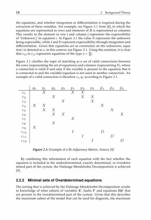
From earlier it is clear that the analysis done by structural methods, or structuralanalysis, does not rely on what type of analytical expression that combines thevariables to a specific equation. Instead, structural analysis is performed basedon the set of unknowns X, the set of known signals Z and the set of faults F, ormore specifically, the subset of each of those sets that are present in each of themodels equations. Each equation in the system contains a subset of elementsfrom each of these sets. The expressibility of these element in each equation isdescribed by the Bi-Adjacency Matrix, that is, what variables that exist in each of


the equations, and whether integration or differentiation is required during theextraction of these variables. For example, see Figure 2.1 from [8], in which theequations are represented as rows and elements of X is represented as columns.This results in the element in row i and column j represents the expressibilityof ’Unknown j’ in equation i. In Figure 2.1 the value X represents the unknownbeing expressible, while I and D represent expressibility through integration anddifferentiation. Given that equations act as constraints on the unknowns, equa-tion i is denoted as ci in this context, see Figure 2.1. Using this notation, it is clearthat c10 to c12 represents equations of the type x = dx

dt .

Figure 2.1 clarifies the topic of matching as a set of valid connections betweenthe rows (representing the set of equations) and columns (representing X), wherea connection is valid if and only if the variable is present in the equation that itis connected to and the variable/equation is not used in another connection. Anexample of a valid connection is therefore c1, q1 according to Figure 2.1.

Figure 2.1: Example of a Bi-Adjacency Matrix. Source [8]

By combining this information of each equation with the fact whether theequation is included in the underdetermined, exactly determined, or overdeter-mined part of the system, the Dulmage-Mendelsohn Decomposition is achieved[8].

2.2.2 Minimal sets of Overdetermined equations

The sorting that is achieved by the Dulmage-Mendelsohn Decomposition resultsin knowledge of what subsets of variables X’, faults F’ and equations EQ’ thatare present in the overdetermined part of the system. Given that this describesthe maximum subset of the model that can be used for diagnosis, the maximum

2.3 Residuals 11

detectability is obviously given by F’. In order to achieve isolability, decouplingis necessary, see Section 2.1.1. Given the following assumption from [8]

Each fault is present in only one equation (2.13)

, all sets that are containing a minimal amount of equations while remainingoverdetermined are of great interest, as they achieve the full decoupling potential.A set that fulfils this property is known as a Minimal set of Overdeterminedequations (MSO). An example of an MSO is the set of equation (2.6) and equation(2.7).

2.3 Residuals

The role of residuals has been discussed throughout this thesis. Before the pro-cess of residual generation that was used in this thesis is described however, athorough background on the residual-subject must be given. This includes thetheoretical definition as well as properties of residuals that are worth consideringwhen constructing a diagnostic system. One certain preconditions that must bemet when constructing residuals is that the included equations must compose anoverdetermined system, which follows from the definition of redundancy givennext.

Definition 3. [18] There exist analytical redundancy if there exist two or more differentways to determine a variable x by only using observations z, that is x = f1(z) and x = f2(z),where f1(z) . f2(z).

By using the definition of analytical redundancy from Definition 3, the follow-ing general expression of a residual can be formed;

r = f1(z) − f2(z) (2.14)

From equation (2.14) it follows that r , 0 provides an observation that is differentfrom the observation when the system is in a faultfree mode. This enables isola-tion from the mode according to Definition 1. This specific isolability is identicalto detectability.

The analytical redundancy can occur both as static redundancy and temporalredundancy. Static redundancy corresponds to f1 and f2 not containing any dif-ferential operators, that is, no numerical integration or differentiation of the ele-ments in z are necessary. Temporal redundancy means the opposite; that at leastone numerical integration or derivation is necessary of the known quantities inorder to achieve the residual. Whether a redundancy is temporal or static is ofgreat importance as it effects the properties of the computed residual. One ofthese properties is causality which is covered in Section 2.3.1.

2.3.1 Sequential residuals

As previously stated in this thesis, only overdetermined set of equations can beused for generation of residuals. This follows from the definition of redundancy,


Definition 3. In an underdetermined or exactly determined system, there is onlyone way (at the most) to describe each unknown quantity. This means that thereis no redundancy, and therefore no residual can be generated. Sets that doesnot contain any underdetermined or exactly determined parts are therefore ofgreat interest, these sets are known as Proper Sets of Overdetermined Equations(PSOs).

If the system S is overdetermined however, then there are multiple subsystemsS ′ that are exactly determined and contains all unknowns of S. This means thatevery unknown variable in S ′ can be expressed using S ′ alone. By substitutingthe unknown variables in S\S ′ with these expressions, the redundancy of Defini-tion 3 is achieved.

If the redundancy is temporal, then numerical integration, differentiation or acombination of these must be applied to the known quantities of S in order toachieve a residual. This corresponds to the residual having integral , derivativeor mixed causality. Selecting S ′ therefore effects the causality of the resultingresidual, given that the redundancy is temporal. If the redundancy is static how-ever, no differentiation or integration of the known quantities is necessary. Giventhat only algebraic substitutions are sufficient for residual generation in this case,the causality is called algebraic. For more information regarding the definitionof causality, see [8].

2.3.2 Observer based residuals

While the implementation of sequential residuals is straight-forward, it is alsosensitive to measurement noise. One way to suppress this noise is by followingthe methodology described in Section 2.4 assuming that an overdetermined sys-tem with non-algebraic causality is available. This system can be written in theform of equation (2.17), from which the residual can be computed as the estima-tion error.

2.4 Observers

When estimating a certain quantity in a system that is modelled, there are twosources of information in the general case. The first source is the model itself.By initiating the model with an estimation of the current state of the system,certain prediction of the systems behaviour can be achieved by simulating themodel. Relying on this source alone however, results in high demands, both onthe accuracy of the model and the ability to estimate the initial state of the system.Given that the initial state can be regarded as an unknown quantity, this resultsin a situation where the estimation method only can provide accurate estimatesif certain accurate estimates are already given. This situation is resolved by usingthe second source of information, which consists of the measurements providedby the sensors of the modelled system. The combination of these sources results

2.4 Observers 13

in an estimator with maintained predictive ability and less dependency of theinitial state estimate. This combination is achieved by an observer. Consider thefollowing linear state space model

x = Ax + Bu

y = Cx (2.15)

where x denotes the state, u denotes the input and y denotes the measurements.The coefficients A, B and C are matrices that describes how the previous denotedquantities are connected. Let x denote the estimated state. By utilizing the modelfrom equation (2.15) and using proportional feedback from the difference be-tween measured y and estimated measurements Cx, also known as the estimationerror, correction of the estimated state can be achieved. The gain of the propor-tional feedback; K , is known as the observer gain. Based upon this informationthe observer can be defined as the following;

˙x = Ax + Bu + K(y − Cx) (2.16)

The resulting observer of equation (2.16) is clearly depending on the model of thesystem, the provided measurements and the observer gain K . The details of de-termining K is not treated in this thesis, but is referred to other implementations,such as the continuous variance-minimizing Kalman filter [2].

2.4.1 Observers of Non-Linear Systems

Unfortunately, far from all systems are linear and on state-space form such asthe system in (2.15). Now consider the following non-linear differential algebraicmodel

x1 = f (x1, x2, z, t)

0 = h(x1, x2, z, t) (2.17)

where the unknown variables x has been split up into the state variables x1 andthe algebraic variables x2. The known signals, such as measurements and inputsare described by z.

In order to achieve an observer with desired behaviour the nonlinearities mustbe handled in some fashion. The easiest method would include simplification ofthe model by expressing x2 as a function of x1, t and z followed by a linearizationof the model. Then the Kalman filter can be applied to these linearized models,which results in the Extended Kalman filter described in [10, Chapter 7].

Before discussing the observer implementations used in this thesis, a backgroundon Differential Algebraic Equations (DAEs) and more specifically their index isneeded. An example of a DAE is seen in equation (2.17), however, as stated in[14] the equations must not necessarily have the derivatives expressed explicitlyas in equation (2.17). The index of the DAE corresponds to the number of differ-entiations needed in order to achieve that expressibility according to [14]. Based


on these definitions of DAEs and index, the observer implementation can be spec-ified.

This thesis uses the observer implementation described in [12], see equation(2.18). This is motivated by the fact that the current implementation of observersin the FDT only supports low-index problems (index=1), which is complementedby the index-reduction capabilities of the method described in equation (2.18).

Background on Method for Non-Linear Observers

Similar to the regular observer in equation (2.16), the method presented in thissection uses feedback from the estimation error r in order to minimize the differ-ence between the estimated and measured state. The difference from many sim-pler applications, such as those described in Section 2.4 is that this method usesa feedback based on the estimation error r with both proportional and derivativeterms. Based on the model seen in (2.17), this results in the following system

˙x1 = f (x1, x2, z, t) + F(t)r + G(t)r

0 = h(x1, x2, z, t, r) (2.18)

where the coefficients G(t) and F(t) provide proportional and differential feed-back in the constructed observer, and the specific presence of r in h is left aschoice of design. In this thesis, the method presented in [12] is used to determinethe coefficient F(t). As seen in equation (2.18) this method utilizes the informa-tion from the estimation error by using feedback provided from a PD-controller.By selecting the coefficients of the controller according to Theorem 1 and Theo-rem 2 in [12], low-index and asymptotic stability can be guaranteed. In this thesishowever, only theorem 1 will be used. Before the theorem is given, let hx denotethe gradient of h with respect to x and N (A) denote the right null space, that is{x : Ax = ~0}.

Theorem 1 Given a model in the form of equation (2.17) a low-index observeron the form of equation (2.18) can be guaranteed if the following criterions aremet.

1. hx have full row rank for all x.

2. hx2must have full column rang for all x2.

The first criterion corresponds to no rows in the gradient of h being linearly de-pendent. The second criterion corresponds to the requirement that every com-ponent of h, must have derivatives based on elements from x2 such that thesederivatives results in columns that are linearly independent of each other. Or, inless mathematical terms, that it is possible to solve for x2 in the algebraic part ofequation (2.17).

The criterions mentioned so far are prerequisites and doesn’t reveal any informa-tion regarding the specific design of F(t). This is described by the third criterion,

2.5 The Optimal Control Problem 15

stated below. Let N denote the null space. Also, let V and W be defined in thefollowing manner

V = { x1 : ∃x2 : (x1, x2) ∈ N (hx) } (2.19)

W = { x1 : x1 < V } (2.20)

If the previous requisites are fulfilled and= F(t) = W (the Image of F(t) = W),then the resulting observer is low-index which concludes Theorem 1 from [12].The proof of this theorem is found in [12].

2.5 The Optimal Control Problem

Similar to the chess player planning their next move, the field of optimal controlseeks the optimal sequence of actions. Expressing these actions or controls asfunctions of the current state or current position of the pieces on a chessboard ifyou wish, is known as expressing a policy. Finding an expression for the optimalpolicy is the main goal in the field of optimal control. It must however be spec-ified in what way a certain policy is optimal. This information is found in theformulation of the optimal control problem

min .u(.)

φ(x(tf )) +

tf∫ti

f0(t, x(t), u(t))dt subject to

x = f (x(t), u(t))u(t) ∈ U ∗x(t) ∈ X∗

(2.21)

which in the content of this thesis got a predetermined initial time ti and end timetf . While the problem described by equation (2.21) looks very complex at firstsight it is basically a consideration between the penalty of effort, measured bythe integral-part of the objective function and the penalty of final performance,which is measured by φ. For the chess-player for example, ending in the state ofhaving the opponent in checkmate, is a very successful state to achieve. Thereforeit should correspond to a very low value of φ. With similar reasoning, ending upbeing checkmated by the opponent should correspond to a high value of φ. Sim-ilar to chess, the state and control signal cannot change in an arbitrary fashion,there are a set of constraints or rules regulating what states and control signalsthat are valid. These constraints are mathematically described by X∗ and U ∗ andcorresponds to the chess player not being allowed to have pieces outside of theboard or move diagonally with the knight for example.

When solving the problem described in equation (2.21) the field of optimal con-trol provide two general analytical methods that are applicable to the given prob-lem. The Hamilton-Jacobi-Bellman equation (HJBE), which provides sufficientand necessary conditions for optimality and the Pontryagin’s Minimum Principle(PMP), which only provides necessary conditions for optimality [25]. In this the-sis only PMP has been used, and therefore the focus will remain on this methodfrom this point on.


2.5.1 Pontryagin’s Minimum Principle

The mathematical process of optimization is often simple, given the context of theupper secondary school. A typical approach is differentiation of the non-linearobjective function and comparing all values of the objective function that arisesfrom the zeros of this derivative. However, when optimizing with constraints, asin equation (2.21), the complexity of the problem suddenly rises above the levelof upper secondary school.

When the constraints consists of an state space model, Pontryagin’s MinimumPrinciple (PMP) enables calculation of candidates for an optimum in a similarfashion to the derivative-solution above. The clearest similarity is that PMP alsoprovides necessary (but not sufficient) requirements for optimums. It is thereforeonly used to compute candidates which must be compared manually in order toverify the optimum.

Hamiltonian and Equations

The computation of the optimum of equation (2.21) must somehow take both thegoal-function and the constraints into account. PMP solves this matter by com-bining the f0(t, x(t), u(t)) with the differential constraint of the state f (x(t), u(t))with the help of the adjoint variable known as λ. This combination is describedby the Hamiltonian;

H(x(t), u(t), λ, t) = f0(t, x(t), u(t)) + λ · f (x(t), u(t)) (2.22)

Given that λ has been introduced, additional equations must be added in orderto achieve a solvable equation system. The resulting equation system is

Constant = min .u(.)

H(x∗(t), u∗(t), λ, t) (2.23)

λ = −Hx (2.24)

λ(ti) ⊥ x∗(ti) (2.25)

λ(tf ) − ∇φ(x∗(tf )) ⊥ x∗(tf ) (2.26)

For more information see [9]. In this thesis, only the pointwise minimizationfrom equation (2.23) and the adjoint equation from equation (2.24) will be used.Given that equation (2.25) and equation (2.26) only provides information regard-ing the specific initial and termination values of x and λ the loss from excludingthese equations are considered minimal.

2.6 Summarized Roadmap of Background Research

The investigation of the issues in Section 1.2 is dependent on access to relevantand suitable scientific sources. This section gives a general summary of the the-ory used in the project and also points to adequate sources on the respective field.

2.6 Summarized Roadmap of Background Research 17

As stated in Chapter 1 model based diagnosis refers to modelling a system andto build the diagnostic system based on that model [18]. This typically results ina number of equations that capture the main behaviour of the modelled system[14]. When applying structural methods however, as described in Chapter 1 and[13], only the model structure is relevant.

Of the equations describing the system, only certain equations can be used fordiagnosis, the equations that form overdetermined equation systems. One wayto compute this equation set is to use the Dulmage-Mendelsohn composition,which is described in [8]. However [8] also states that there can be smaller overde-termined subsets of this set known as minimal sets of overdetermined equations,MSOs. As these sets are minimal, it follows that they contain exactly 1 moreequation than unknown variables. The paper [11] shows examples of algorithmswhich find these sets and compares them with respect to complexity.

While knowing the information provided by the MSOs is sufficient for generatingall possible residuals of a system, additional information is needed in order to ac-tually generate residuals. The paper [4] shows an implementation on this topic.The application in [4] resulted in residuals with mixed causality. The causalityof residuals is described according to [8] by what type of calculations; differenti-ation, integration, that are necessary for achieving the residual. As stated earlierall MSOs consists of 1 more equation than the number of unknowns, removal ofone equation, ei from the set will result in an exactly determined equation sys-tem. This means that all of the unknown variables in the MSO are computableand thus computing them and substituting the unknown variables in ei results ina residual-equation. However this substitution may result in demands for numer-ical integration, derivation or a combination of these, which results in integral,derivative or mixed causality. In the event that none of these options are requiredfor the substitution, the causality is called algebraic.

The computation may include solving of Diffential Algebraic equations (DAEs),which is described in [14] as general equations involving variables and theirderivatives. [14] also describes the index of a DAE as the number of times theDAE must be differentiated in order to achieve state space form. High-indexDAEs are typically harder to solve according to [6, 22], although [22] describedan algorithm for computing the largest low-index subpart of a high-index DAE.There are also examples of algorithms that converts high-index DAEs to low indexdirectly, see [21]. If the problem is low-index then according to [6] an observerbased residual can be constructed in the current observer-implementation. Con-struction of observer based residuals based on a non-linear differential equationis described in [12].

While causality and index describes the mathematics required to compute a diag-nostic system, it doesn’t describe the properties of the achieved diagnostic systemitself. One such property is isolability, which according to [18], describes the abil-ity to exclude other faults when in presence of a specific fault. More details on


isolability can be found in [16, 20], while [19] contained an algorithm for evaluat-ing the property.

The resulting properties, such as the isolability of the diagnostic system, are de-pendent on the tests chosen to be included in the diagnostic system. There arecertain limitations on test selection in order to satisfy demands for isolability,this topic is treated in [3, 17]. The paper [3] covered an efficient way of reducingthe search-space by taking the realizability properties into account. Accordingto [3] the method was also applied successfully to an industrial sized automotiveengine system. The paper [17] on the other hand describes an algorithm for deriv-ing MSOs. The article states that the algorithm has polynomial complexity andtherefore is more suitable for industrial examples than other algorithms.

A necessary condition for having any isolability or detectability, i.e isolabilityfrom not having any fault; is redundancy. According to [18] redundancy meanshaving more equations than unknowns, which basically is resulting in the overde-termined equation system discussed earlier. One way to affect the number ofequations is placement of certain sensors, this topic was covered in [7]. In [7]it was also stated that adding new sensors enables transition of equations fromthe exactly determined part of the Dulmage-Mendelsohn decomposition to theoverdetermined part. Furthermore, based on the model structure, minimal setsof sensor placements for full detectability can be computed and similar algorithmis also applicable for isolability according to [7].

When adding sensors however, it’s important to consider the Signal-to-Noise-Ratio (SNR) itself as well as its size relative to the precision of the equations of themodel. The topic of extracting as much information as possible from a set of sen-sors when in presence of noise is called sensor fusion. In sensor fusion one of thefundamental algorithms, Weighted Least Squares, provides a way to valuethe received information with respect to its certainty. This algorithm is describedin [10].

3Background

The background of the thesis is presented in this section. As stated in Chapter1, the key concept of the diagnostic system computation is translation/parsingof Dymola Models into Matlab. In order to achieve this, an understanding ofthe Dymola language Modelica is needed, this is provided in Section 3.1. Thetranslation process involves the XML-format, which is briefly covered in Section3.2, and a translation program (parser), which is covered in Section 3.3. Theparser was developed during the thesis but is founded on the work in [15]. Theparser is applied to the CPC model, which is introduced in Section 3.4.1, the twotank model in Section 3.5.1 and the SECS model presented in Section 3.6. Givena correct translation of these models, the FDT can be applied in order to computea diagnostic system, the FDT is covered in Section 3.7.

3.1 Modelica

The language used in Dymola is called Modelica. Modelica is a equation-orientedprogramming language, where basically a list of equation describes the behaviourof the model based on given parameters and variables, see Figure 3.1. Similar tomany other languages, the left part of the declaration declares the type while therest specifies the name. Also note that all variables and parameters must be de-clared before they are used [14]. The equations using these parameters and vari-ables are specified under the line ’equation’. When adding variables, equationsor parameters, the line must be terminated by a semicolon. Suggested initial val-ues of variables can also be added in the declaration by adding (start = value)to the declaration, where value is the suggested value. Any declarations of pa-rameters/variables and definitions of the equations must all be within the limitsof the model, which is marked by ’model model-name’ and ’end model-name’. Forclarification see the example in Figure 3.1.

19

20 3 Background

model Rocketparameter Real losses=0.1;

Real velocity(start=0);

Modelica.Blocks.Interfaces.RealInput thrust;

equationder(velocity) = thrust*(1-losses);

end Rocket;

Figure 3.1: Modelica code example that explains variables, parameters andequations

3.1.1 Re-usage of Code

According to [14] Modelica also includes model-libraries which enables the us-age of model-objects as a sub-model of new models. By defining and saving thedefinition of modelx as in Section 3.1, the addition of the line modelx modelx_1;will add an modelx object with the name modelx_1. See the example in Figure 3.2where Rocket objects called Rocket_1 and Rocket_2 are added. The partial prefixof the model indicates that the model can be expanded using inheritance, seeFigure 3.3. Defining model-objects in this manner, having model-objects inside

partial model Rocket_fleetRocket Rocket_1;Rocket Rocket_2;end Rocket_fleet;

Figure 3.2: Modelica code example that explains re-usage of models

other models, results in a hierarchical model. The hierarchy in the hierarchalmodel is refering to the fact that the variable x from inside the modelx objectis different the variable x being on the same level as the modelx object. Theselevels are here refereed to as the hierarchy and are also exemplified in the givenexample, as the Rocket_fleet model contains Rocket objects.

Connectors

One of the greater benefits of Modelica is the possibility to reuse older modelsin different applications. This is achieved by defining objects of different modelsand connecting them. In order to transfer data between model objects, an ele-ment called connector must be used. Connectors enables connection of differentmodels by specifying an interface, which then can be used in connect-statements,see the example in Figure 3.3.

3.2 eXtensible Markup Language, XML 21

Inheritance

Modelica also includes the possibility of inheritance. By defining a model as apartial model and using the command extend, all the source-code from insidethe limits of the model in Section 3.1 is pasted at the location of extend model-name;. Both connectors and inheritance is treated in the example of Figure 3.3.

model complete_fleetextend Rocket_fleet;

Modelica.Blocks.Interfaces.RealOutput order_1=1;Modelica.Blocks.Interfaces.RealOutput order_2=-1;

equationconnect(Rocket_1.thrust,order_1);connect(Rocket_2.thrust,order_2);

end complete_fleet;

Figure 3.3: Modelica code example that explains re-usage of models usinginheritance and connectors

3.1.2 Algorithms

As mentioned earlier, models are described by equations, where the left handside of the equality sign is equal to the right hand side of the equality sign. Theorder of operands doesn’t matter given that equality is a symmetric relation, a =b ⇐⇒ b = a. That symmetry can be avoided by using the assignment operator,:=, instead. This and similar operations, where the purpose is to specify whatcomputations to be done, rather than declaring a model, is written in a sectioncalled algorithm. Algorithms typically also contains traditional loops such as forand while.

3.2 eXtensible Markup Language, XML

An XML document simply stores information marked up in a text by using tags.Tags are defined by < name > where the name-part of the tag is describing the in-formation content in the XML-element, which is defined by < name > content </name >. Below this section an clarifying example XML document is given. Thefirst two lines of the file only states that the given file is an XML file and providesa given parser with validation file called ’persons.dtd’. The rest of lines describesthe content, which was the main focus of this project.

22 3 Background

<?xml version="1.0"?><!DOCTYPE persons SYSTEM "persons.dtd"><persons><person job="programmer"><name> John Doe </name><email>[email protected]</email></person>...<person job="manager"><comment>Classified<\comment></person></persons>

Similarly to the example above, other types of information can be stored inthe XML format. One type is model information from a Modelica model whichcan be extracted from Dymola in XML. Information-content from the model isstored in an XML-tree, which can be translated into any programming languageusing a designated parser.

3.2.1 Hierarchy

When processing data from an XML-file, it’s important to consider where in thestructure the data has been found. This information of location of data is calledHierarchy in this thesis, as it follows from the similarity to hierarchial models insection 3.1. In this example the importance of hierarchy is clearly shown, as theinformation stored in email is useless unless you also got access to the informa-tion of who the email belongs too, which is stored in the hierarchy leading to thespecific email element.

3.2.2 XML-generation in Dymola

A Dymola model can be generated as a file with the format XML [5]. For example,the commando Advanced.OutputNestedExpandedModelAsXML: enablesgeneration of XML-file where the hierarchy of the model is maintained. Pleasenote, that according to the developer of Dymola, Dassault, the XML-generation ofDymola is under development and might change in future releases. The Dymolaversion used in this thesis is 2018 alpha, see Table 1.1.

3.3 Parser

A basic parser was implemented by K. Lockowandt see [15]. The parser enabledconversion of models from the XML-format to .mat-format, which is fundamen-tal to the method of this thesis, see Item 1 in Section 4. More specifically, the fileformed in the .mat-format defines a Diagnosis Model object, which the FDT canbe applied to, see Section 3.7.

The parser was developed further during this thesis, which enables handling of

3.4 Cabin Pressure Control 23

matrix-variables, if-equations and for-loops, as well as handling of the case ofhaving the same fault in multiple equations. For more information on the parser,see Appendix A or [15, chapter 5, p 17].

3.4 Cabin Pressure Control

Given that an air-plane such as Gripen cannot operate without a ’functioning’ pi-lot, certain systems must be operable in order to ensure that the pilot remainsin this state. One of these systems is Cabin Pressure Control (CPC), shown inFigure 3.4. The CPC controls the cabin pressure and consists of a Cabin PressureController which is connected to two discharge valves [23]. The discharge valvescontrols the mass flow rate between the cabin and the ambient pressure by chang-ing its position. The desired position is achieved by comparing a provided servopressure with the cabin pressure, this comparison enables the discharge valves tochange their position and therefore realize the shift in cabin pressure. The CabinPressure Controller provides the servo pressure to the valves and therefore con-trols the shifting of cabin pressure, which explains the name of the component.It is worth noticing that the connection between the controller and the dischargevalves is mechanical [24], see the discharge valves in Figure 3.4.

Figure 3.4: A system overview of the Cabin Pressure Control

3.4.1 Cabin Pressure Control model

A physical model of the CPC in Gripen E/F has been developed by Saab and im-plemented in Dymola using components from “Modelica Standard Library” [24].The model of the discharge valve describes the mass flow rate from the cabin tothe ambient as a function of the pressure difference, the valve loss characteristics,and the opening area. The opening area is determined by a balance of the forcesacting on a rolling diaphragm. By dividing a part of the internal volume into twochambers, P1 and P2, which are connected to this diaphragm using pistons, vari-ation of the position/lift of the valve can be achieved by the pressure provided toP1 and P2. Both P1 and P2 produces forces that effects the position of the valve.

24 3 Background

These forces also opposes each other, which means the resulting position of thevalve is related to the relation of the pressures of both chambers. By connectingP1 to the servo pressure, and P2 to the cabin pressure, the position of the valvecan be controlled in a desired manner [24]. An overview of the entire CPC modelis seen in figure 3.5.

Figure 3.5: Overview of the CPC model

In Figure 3.5 the cabin is represented as the volume in the lefthand side ofthe model. The pressure of this volume is then regulated with respect to the pres-sure in the ambient volume in the opposite side of the model by the connectionthrough the discharge valves. In order to achieve a valid representation of thedischarge valves, the diaphragm is modelled as a spring and damper in parallel.This is connected to a mass with movement restrictions adapted to the possibledisplacement of the real valve.

3.5 Two Tank System

A simple model is necessary in order to enable testing of the developed algo-rithms as well as providing additional support for any conclusions made regard-ing diagnostic system generation. For these purposes, the two tank system, illus-trated in Figure 3.6 is introduced. The system includes two tanks with orifices atthe bottom of each tank, a pump, and sensors that measures the water levels ofthe tanks; x1 and x2.

3.5 Two Tank System 25

Figure 3.6: Schematics of the coupled two-tank system. Source [15]

In addition to the sensors measuring x1 and x2, there are also flow measuringsensors, see Table 3.1.

Table 3.1: Initial sensors in the two-tank system.

y1 Water level in tank 1.y2 Water level in tank 2.y3 Water flow between tank 1 and 2.y4 Water flow out of tank 2.

3.5.1 Two Tank Model

The model of the Two Tank System is computed by using the physical relationknown as Bernoulli’s principle, which relates the outflow from an orifice at thebottom of a tank to the current water level. Assuming that the cross section areaof the tank is contant, Bernoulli’s principle states the following

v(t) =√

2gh(t), (3.1)

where the water level is denoted by h, the water flow speed by v and thegravity is described by g. Furthermore the relation between the outflow from thetank q(t) and the water flow speed is given by

26 3 Background

q(t) = av(t), (3.2)

where a denotes the area of the orifice through which the water flows out ofthe tank. From the assumption regarding constant base area, it is clear that thevolume of the water contained in the tank is described by Ah(t) where A is thecross sectional area of the tank. The rate of which the volume changes over time,i.e the time derivative, is

Ah(t) = u(t) − q(t), (3.3)

i.e the flow into the tank (u(t)) subtracted by the flow out of the tank. Equa-tion (3.1)-(3.3) gives an explicit expression of the water level in the tank:

h(t) =1Au(t) −

a√

2gA

√h(t). (3.4)

Given that there are two water levels to monitor in the given system, one statefor each water level is introduced. These are denoted x1 and x2 for simplicity.From the previous calculation, the derivatives of these states can be explicitlyexpressed and therefore the computation of the state space model is complete.The complete state space model is

x1(t) =1A1u(t) −

a1√

2gA1

√x1(t) (3.5)

x2(t) =a1√

2gA1

√x1(t) −

a2√

2gA2

√x2(t). (3.6)

y1 = x1 (3.7)

y2 = x2 (3.8)

y3 = a1√

2gx1(t) (3.9)

y4 = a2√

2gx2(t) (3.10)

where equation (3.5) and (3.6) describes the dynamics of the entire system, whilethe measurements are described by equation (3.7) to (3.10).

The model description from equation (3.5) to (3.10) can now be expanded byintroducing fault signals, i.e. variables that represents physical faults, such asblockage or leakage for instance. In this application the faults described in Table3.2 are introduced.

3.6 Secondary Enviromental Control System 27

Table 3.2: Faults introduced in the two-tank system.

fClogging1 Blockage between Tank 1 and Tank 2.fActuator Discrepancy in the Pump.fLeakage2 Leakage between the water-flow sensor of Tank 1 and Tank 2.fWaterLevel2 Measurement error in the water-level sensor of Tank 2.fFlow1 Measurement error in the water-flow sensor of Tank 1.fLeakage3 Leakage between Tank 2 and the water-flow sensor of Tank 2.

By introducing the faults of Table 3.2 in the model described by equation (3.5)to (3.10), the complete model is achieved;

x1(t) =1A1u(t) + fActuator −

a1√

2gA1

(1 − fClogging1)√x1(t) (3.11)

x2(t) =a1√

2gA1

(1 − fClogging1)(1 − fLeakage2)√x1(t) −

a2√

2gA2

√x2(t) (3.12)

y1 = x1 (3.13)

y2 = x2 + fWaterLevel2 (3.14)

y3 = a1√

2gx1(t)(1 − fClogging1) + fFlow1 (3.15)

y4 = a2√

2gx2(t)(1 − fLeakage3) (3.16)

Given that fClogging1 exists in multiple equations, the assumption from 2.13 isnot fulfilled. There are however, tricks to bypass this problem, which is coveredin Section 3.7.

3.6 Secondary Enviromental Control System

The Secondary Enviromental Control System (secs) in Saab 39 Gripen fulfillsthe function of supplying electronics and radar with cooling air. Hot air from theengine is processed in the system, consisting of two coolers in series with a turboelement that connects the two coolers, see Figure 3.7. This model was also usedin a parallel thesis, see [15], and the description of the model from that thesis isgiven in the next section for simplicity.

3.6.1 Model of the Secondary Environmental Control System

To model the air supply and cooling system, i.e the Environmental Control Sys-tem (ecs) of the air-plane Saab 39 Gripen, Saab uses the modelling languageModelica. The ecs can be divided into a Primary (pecs) system, a Secondary(secs) system and a Liquid Loop (ll), allowing each sub-system to be modelledseparately. For different purposes more or less detailed models of the system isnecessary. Therefore a detailed high fidelity (hfm) and a reduced low fidelitymodel (lfm) was developed. The hfm is used mainly for testing performancerequirements, while the lfm is mostly used in simulators. This thesis focusesmainly on the secs lfm.

28 3 Background

Model Description

In Figure 3.7 the main part of the secs-model is depicted. Hot and pressurisedair is taken from the engine and cooled down. The cold air is used to cool downthe liquid in the ll, which in turn is used to cool equipment, not depicted in theschematics. Three types of sensors are used to monitor the system, namely tentemperature sensors, four pressure sensors, and one accelerometer. The highamount of sensors monitoring the system makes the model useful for model-based fault diagnosis.

Figure 3.7: Schematic of the Secondary Environmental Control System.

3.6 Secondary Enviromental Control System 29

3.6.2 Addition of Monitored Faults

Based on a request from Saab the faults of Table 3.3 are implemented into themodel in order to achieve a hint of the current diagnosis potential in the system.

Table 3.3: Faults introduced in the SECS

fmFlowEjector Deviating mass-flow through the ejectorfmFlowP recooler Deviating mass-flow through the precoolerfetaP reCooler Deviating degree of efficiency in the precooler.fmFlowP ack Deviating mass-flow through the cooling packfetaT urb Deviating degree of efficiency in the turbine

The faults presented in Table 3.3 are marked in Figure 3.8, as the model is con-fidential, a more detailed explanation of what specific equations that are effectedof the fault cannot be given.

Figure 3.8: The SECS model with faults of Table 3.3 implemented

30 3 Background

3.7 Fault Diagnosis Toolbox

The Fault Diagnosis Toolbox (FDT) is implemented in Matlab and enables compu-tation of a diagnostic system based on a model of the diagnosed system. The FDTuses structural analysis to decide which equations that should be used in eachresidual. In the current version (2016-12-22) each fault must exist in only oneequation as addressed in [6]. Given that the model description of the Two TankSystem (3.11) - (3.16) does not fulfill this, either the chosen model or the chosenmethodology (FDT) must be modified. In this thesis, the trick from 2.13 is used,which means that each of the faults that are present in many equations are sub-stituted with a new unknown variable. This would result in a loss of redundancyif it was not for the fact that an additional equation also is introduced for each ofthese faults. These equations state that the substitute-variables are equal to thefaults that they substitute. For the Two Tank System the adequate change can beachieved by adding the following equation

fClogging1 = f ault0 (3.17)

where f ault0 is the new fault signal, and fClogging1 is just a conveniently namedvariable.

By adding specifications that are redundant from a mathematical point of view,but necessary from a structural viewpoint; namely xi(t) = dxi (t)

dt , the model of theTwo Tank System can be written in FDT compatible form. Having the model inthis form

x1(t) =1A1u(t) + fActuator −

a1√

2gA1

(1 − fClogging1)√x1(t) (3.18)

x2(t) =a1√

2gA1

(1 − fClogging1)(1 − fLeakage2)√x1(t) −

a2√

2gA2

√x2(t) (3.19)

y1 = x1 (3.20)

y2 = x2 + fWaterLevel2 (3.21)

y3 = a1√

2gx1(t)(1 − fClogging1) + fFlow1 (3.22)

y4 = a2√

2gx2(t)(1 − fLeakage3) (3.23)

fClogging1 = f ault0 (3.24)

x1(t) =dx1(t)dt

(3.25)

x2(t) =dx2(t)dt

(3.26)

enables clarification regarding syntax and functions of the FDT, which will aidthe explanation of the implemented algorithms.

A model-object for the model described by (3.18) to (3.26) will now be specifiedin Matlab using the FDT. The FDT must have access to the information whether

3.7 Fault Diagnosis Toolbox 31

a variable is part of the unknown variables, known variables, or fault variables,which corresponds to the variable being part of X, Z, F respectively. For thismodel, this specification corresponds to the Matlab code provided in Figure 3.9,assuming that the prefix d is used to indicate a derivative.

modelDef.x={dx1,x1,dx2,x2,f_{Clogging1}};modelDef.f={fault_0,f_{Actuator},f_{Leakage2},f_{WaterLevel2},...f_{Flow1},f_{Leakage3}};modelDef.z={u,y_1,y_2,y_3,y_4};

Figure 3.9: Short example of definitions used for the FDT

The parameters and model equations are entered in a similar manner, see [6].The FDT supports two kind of models, symbolic and structural, where a symbolicmodel contains a complete model, while a structural model only contains thestructure of a model. Given that the entire Two Tank System model is available,both structural and symbolic model objects can be created for this model usingthe FDT. For more information regarding the methods available for the createdobject see [6, p. 4] or the matlab commando methods DiagnosisModel.

4Method

This section treats the methodology used in the project. In order to distinguishbetween the methods that were pre-existent to the thesis, and those that wereinvented during the project, any method mentioned is considered invented unlessstated otherwise. The general methodology can be concluded in the followingpoints, see the following subsections for further information.

1. Convert the model from Dymola to Matlab.

2. Analyze the model using the FDT.What can be said about the model index, MSOs, causality properties?

3. Extract the desired parts, that is the MSOs that will result in a diagnosticsystem that has sufficient detectability and isolability.

4. Analyze which type of residual, that results in desired behaviour for thecurrent application; observer, sequential or other type.

5. Generate residuals based on the selected MSO-sets.

6. Convert residuals from Matlab to Dymola and compare the results of theresiduals.

4.1 Processing of Model using Fault DiagnosisToolbox

The idea is to convert the model from .mo to .mat format by using a parser devel-oped in Python. Once the model is converted into matlab, the FDT can be usedto compute the MSOs. These MSOs are analyzed and sorted such that the cho-sen subset of the MSOs results in residuals with sufficient isolability and as high

33

34 4 Method

causality as possible. High causality refers to algebraic being prefered before In-tegral which in turn is prefered before mixed causality. Derivative causality isconsidered the lowest based on the experience that differentiating of noisy sig-nals often results in poor accuracy, and therefore should be avioded.

The MSOs chosen by the algorithm are automatically converted into sequentialresiduals. By allowing the FDT to do its test selection on a sorted subset of theMSOs, the isolability and causality of the generated residuals can be guaranteedsimultaneously. The figure 4.1 below describes the general algorithm for gener-ation of a diagnostic system based on a FDT-model object, a set of MSOs, anda desired isolability. Apart from the node Generate tests, which corresponds tothe FDT method TestSelection, the nodes of Figure 4.1 represent algorithmsimplemented in this thesis. The MSO-computation is described in Section 4.1.1,the sorting of the MSOs is described in Section 4.1.2, and the residual generationis described by Section 4.1.3. The resulting residuals generated by this algorithmare then converted into .mo-format, which enables simulation in Dymola.

Figure 4.1: General view of the diagnostic system generation

4.1.1 MSO-computation

Once the description of the model has been converted into Matlab, the FDT canbe used to compute a suitable diagnostic system. As mentioned earlier, only theoverdetermined part of the model can be used to make residuals. This sectiondescribes the computation of minimal overdetermined sets of equations, (MSOs).

The FDT supports computation of all MSOs by using the member-function MSO,see [6]. However, as stated in [6, 17] the complexity of MSO-computation is oftenexponential with regards to the degree of redundancy in the model. Therefore, a

4.1 Processing of Model using Fault Diagnosis Toolbox 35

new algorithm that computes a reduced number of MSOs was developed duringthe thesis.

The algorithm used the method Minimal Test Equation Support, MTES,from the FDT to extract overdetermined subsystems of the original system. Addi-tionally, sensors that did not contribute to the potential detectability or isolabilityaccording to the FDT were removed, which together with extraction resulted inreduced redundancy. By applying the MSO-method on these subsystems, a sub-set of the MSOs, which results in the same potential isolability and detectabilityas the sets generated by the MSO-method, can be computed with a lower timecomplexity.

4.1.2 MSO-sorting

As motivated in the introduction to Section 4.1 desirable properties of the gener-ated residuals are high causality as well as sufficient resulting isolability. Basedupon this a sorting algorithm was developed. This sorting algorithm works in twosteps. First it divides the MSOs into subsets based on the best achievable causal-ity in each MSO. Then it checks whether the subset of MSOs with best causalityalone will result in sufficient isolability. If that is the case then the current sub-set is selected, if not then the subset is expanded by the subset with second bestcausality and the process is repeated until either sufficient isolability is achievedor all MSOs are included. The included MSOs are used for residual generationwhich is covered in the following sections.

4.1.3 Sequential residuals

Sequential residuals are generated using the method seqresgen from the FDT.By removing one equation from the MSO, the number of independent equationsand unknowns are identical in the remaining set, which is a necessary but notsufficient condition for the equation system to be solvable. As it is not sufficient,the validity of the result generated by the solver is tested in the algorithm. Itis also worth noticing that the residuals created by the FDTs seqresgen methodassumes that the derivatives are constant between its state estimates [6], similarto the Euler-forward method.

Removal of MSOs

As stated earlier, the number of independent equations and unknowns beingequal is not a sufficient condition for the system to be (uniquely) solvable. There-fore the algorithm is developed in such a way that if Matlabs solver solve (whichis used in the seqresgen method) fails to find a solution to the equation system,the MSO that was used as input to the method is discarded. In the event that thisresults in the remaining set of MSOs being empty, the algorithm has failed, elsethe sorting and generating process is repeated, see figure 4.1.

36 4 Method

4.1.4 Observer based residuals

Given that the method ObserverResGen from the FDT can only generate ob-servers based on low index problems, another method must be used for problemsof high index. As stated in Section 2.4.1 the method described by (2.18), for com-putation of the D-coefficient (F(t)) in the feedback used in the observer, see firstsubsection of this section. The P-coefficient (G(t)) is computed by using Lanner-hed’s theorem, that will be presented in Section 5.1, in combination with PMP.A summary on the computation of the P-coefficient is provided in the secondsubsection of this section.

Computation of F

From Theorem 1 given in Section 2.4.1, a basic algorithm for computing F(t) hasbeen implemented. The algorithm rewrites the set of equations of an MSO tothe form described in (2.18). Once this step is complete, the symbolic toolbox inMatlab enables calculation of the null space of the gradient of h by solving thefollowing equation;

hx(x1i , x2) ·[x1ix2

]= ~0 , x1i , 0 (4.1)

where x1 represent the states, x1i represents a specific state, and x2 represent thealgebraic variables. Based on equation (4.1) it can be determined what states x1ithat are part of the null space;

A = { i : equation (4.1) fulfilled for x1i }V = ∪x1i ∀i ∈ AW = x1 \ V .

Theorem 1 now states that any F(t) := F(t) = W results in a low-index observer,which completed the computation of the necessary demands on F(t). Note thatthese demands only resulted in limitation regarding the dimension of the coeffi-cient. For simplicity, only ones and zeros were used as elements in F(t) in thisthesis. The flow chart of the algorithm is concluded below.

Figure 4.2: Flow chart, computation of F(t)

The algorithm in Figure 4.2 has similar limitations as the FDT seqresgenmethod, given that the Matlab methods solve and jacobian is used in thecomputation of V , see (4.1).

4.2 Conversion from Matlab to Dymola 37

Computation of G

When Calculating G a different approach is taken. The equations of the chosenMSO are complemented with measurement error r which provides an exactlydetermined equation system which is solvable in Dymola. However, as G is con-sidered to be unknown at this point, at least one additional equation per statemust be added in order to achieve solvability. Instead of calculating G throughlinearization of 2.18 as in [12], an approach based on Pontryagin’s Minimum Prin-ciple (PMP) [9], was used in this thesis.

PMP is used to compute Gi , where i represents the index of each observed state.By utilizing the theory described in Section 5.1, it is shown that the followingequation

Gi =−2fi(x1, x2, z, t) − Fi(t)r

r(4.2)

describes the Gi that results in the integral of (F(t)r +G(t)r)2 being minimal overthe chosen simulation interval. The details of the computation of Gi is foundin Section 5.1.1, while Section 5.1.2 covers the same application with a slightlymodified objective function.

4.1.5 High-index residual implementations

When generating observer based residuals, there is currently no support for high-index MSOs in the FDT according to [6] . However, given that the equations arewritten in the semi-explicit form as in (2.17), the method described in [12] can beused to attempt index reduction. The methodology in Section 4.1.4 can thereforebe used to provide observer solutions to high-index problems. The FDT methodseqresgen is not limited to low-index problems in the same way, and thereforethere is no need to adapt the generation method of sequential residuals to high-index problems.

Given that the sequential residuals can be generated for both high and low in-dex MSOs, these are ideal to use when comparing the performance of the currentMatlab methods of the FDT and the new Dymola methods. This is therefore ofgreat importance to the investigation of Research Question 5.

4.2 Conversion from Matlab to Dymola

Once residuals with desired properties have been generated the last step in thenew method is to convert the corresponding MSOs back to Dymola. This sectioncovers this translation in more detail than previous sections. For clarity, the re-sulting Modelica code of a residual based on (3.21) and (3.23) from the two tanksystem, hereby referred to as the Dymola example, is included below.

38 4 Method

model sequent ia l_2// Parametersparameter Real twoTank_withfaults__a2 = 3 .0000e−02 , twoTank_withfaults__g = 9 .8100e+00;// Var iablesReal twoTank_withfaults__x2 ( s t a r t =6 ) ;// Measured s i g n a l sM o d e l i c a . B l o c k s . I n t e r f a c e s . R e a l I n p u t twoTank_withfaults__y2 , twoTank_withfaults__y4 ;// outputMo del i ca .B loc ks . I n ter fac es .R ea lO utp ut r ;// EquationsequationtwoTank_withfaults__y4 = 2^ ( 1/2 ) * twoTank_withfaults__a2 * ( twoTank_withfaults__g * twoTank_withfaults__x2 )^( 1/2 ) ;twoTank_withfaults__y2 = twoTank_withfaults__x2+r ;end sequent ia l_2 ;

The variables and the parameters are handled in the following fashion; theequations of the chosen MSO is searched for members of the models unknowns,X as well as its parameters. If one of these members are found in the MSO, a corre-sponding variable or parameter are declared as a Real parameter or Real variable.In the Dymola example, the parameters correspond to RealtwoT ank_withf aults__a2and twoT ank_withf aults__g, while twoT ank_withf aults__x2 represent the onlyvariable of the system.

Given that Dymola could not handle overdetermined systems, an additional un-known variable was added in order to avoid singularity. This was achieved bydeclaring a new Real output named r and adding this into the existing equationsystem. By letting r affect only one equation in an additive manner, great simi-larities with the FDT seqresgen method is achieved, as this equation then cor-responds to the resEq-argument of the method, see [6]. The introduction of theresidual variable r therefore fulfilled two purposes. It enabled the achievementof an exactly determined system, which is mathematically necessary, but it alsocaptured the information whether the equations of the MSO were fulfilled or not.As stated in Section 2.14 certain observations z must be provided in order to com-pute the value of the residual. These are declared as inputs in the model object,see twoT ank_withf aults__y2 and twoT ank_withf aults__y4 of the Dymola ex-ample.

By gathering the translated and modified MSO into a new Dymola model, withinput z and output r, a representation of the residual in Dymola was achieved.In order to realize the system, known z must be provided to the model. This isaccomplished by using tables that contains these values and are connected to thecreated model, see Figure 4.3. It is possible to connect the measurements of a sim-ulation directly into the residual object. However, this is not treated in this thesisas the adaptive step-length in Dymola (see Table 1.1) would bias the comparisonbetween the results in Matlab and Dymola, see Research Question 5.

The construction described in Figure 4.3 enables evaluation of multiple residualsat once, and has access to derivative-approximations of the provided measure-ments, which are provided by the combiTimeTables (see [5]). The combiTimeta-bles are then connected to the translated residuals, which will have the form ofthe Dymola example and are represented by the blue boxes to the right in Fig-ure 4.3. In this thesis, the measurements in the combiTimeTables are generatedthrough a simulation of the provided model, although real measurements can be

4.3 Method Discussion 39

inserted and used in the method in an identical manner.

Figure 4.3: Residual Evaluation in Dymola for Two Tank System

4.3 Method Discussion

The current choice of method is a trade-off between applying general algorithmsand being finished within the time-limit of the project. General algorithms en-ables testing of the variety of cases that appears when using multiple models, butit also typically consumes more working hours than more model-specific solu-tions. In order to verify that the algorithm works for the general case and not justa specific model, a variety of models of different complexity are used during thetesting of the algorithm. Applications on simpler models also added certainty tothe results regarding the more general research questions, such as the comparisonbetween the current FDT implementations (Matlab) and the implementations inDymola, see Research Question 5. If only one model would be tested, the risk ofthe results being biased would be much higher. Also, by testing the implementa-tions on multiple models the robustness of the implemented algorithms could besecured. This section will evaluate the advantages and disadvantages of a few ofthe design-choices that were made during the thesis.

4.3.1 Structural Methods

While structural methods enables diagnostic analysis without unreasonable com-plexity there is one serious drawback when using these methods. This drawback

40 4 Method

lies in the fact that the unknown variable x being present in equation ei is a neces-sary but not sufficient requirement for computing and extracting x from ei . Theresult of this being that what is viewed as an exactly determined system froma structural viewpoint might not be uniquely solvable from a symbolic point ofview as mentioned in Section 4.1.3. For example, this situation occurs for all gen-eral linear systems Ax = b where b is a column vector of length n and A is a ntimes n matrix with linearly dependent rows. The implemented method howevermeans that potential information is lost, as sets of equations are discarded. Thisclearly presents a conflict between accuracy and complexity, as evaluating if xreally is extractable from ei increases the complexity, and therefore inhibits themain purpose of using structural methods in the first place.

4.3.2 Causality Sorting

The Causality sorting algorithm is based on the assumption that numerical dif-ferentiation of noisy signals often results in poor accuracy, lower Signal-to-NoiseRatio (SNR) and typically requires lowpass-filtering of the signal. By minimiz-ing the number of numerical differentiations needed in the implementation, theaccuracy-loss is avoided.

4.3.3 Observer Generation

The method chosen for generation of F enables potential index reduction for high-index problems, if the problems are formulated in the semi-explicit form. How-ever, given that PMP is used to calculated the propertional term G, and PMP onlyprovides necessary and not sufficient conditions for optimality, there are poten-tial flaws in the algorithm regarding if a found optimum is global. However oneof the benefits of the PMP implementation is that it is less dependent on a cho-sen operating point compared to other methods, such as the method described in[12] and the method that is currently implemented in FDT, see the FDT methodObserverResGen in [6]. By formulating an optimal control problem, the chosenG is a result of the combination of multiple operating points, which are selectedby Dymolas solver (Dassl) based upon the available measurement data. If an im-plementation requires desired behaviour such as stability in multiple operatingpoints, the PMP method provides a way to allow each operating point to con-tribute in a more even manner compared to linearization, which only takes oneoperating point into account.

Another benefit of the PMP apporach used in this thesis is the properties thatfollows from one of the chosen objective functions

∫ tfti

(F(t)r + G(t)r)2dt. Theseproperties follows from the fact that this objective function reaches its minimumvalue at (F(t)r + G(t)r)2 = 0 ↔ F(t)r + G(t)r = 0, which means that the chosenobserver will regulate r in the following manner,

Fi(t) = 0 =⇒ r → 0 (4.3)

Fi(t) , 0 =⇒ Fi(t)r + Gi(t)r → 0 (4.4)

4.3 Method Discussion 41

where Fi(t) is assumed being a predetermined value.

Equation (4.3) describes the typical desired property of an observer based resid-ual, namely that the residual variable will be pushed towards zero. The proper-ties that follow from equation (4.4) on the other hand states that the behaviourof r will be pushed towards the behaviour of the linear system described byFi(t)r + Gi(t)r = 0. Given that Fi(t) can be set arbitrary (zero excluded), thismeans that the pole of the linear system can be placed arbitrary as well.

4.3.4 Conversion to Dymola

By converting equations to Dymola, high-index DAE problems can be solved [5].According to [5] Dymola enables the usage of a variety of numerical integrationmethods. Although as mentioned in Table 1.1, only the standard Dassl-solver wasinvestigated in this thesis. By looking up the constant eps in the Modelica con-stant library (Dymola 2018 Alpha) and the corresponding coefficient in Matlab(Matlab R2016b) the results in Table 4.1 was found.

Table 4.1: Comparison of machine epsilons Matab/Dymola.

Language Value of epsMatlab 2.2204 · 10−16

Dymola 1 · 10−15

5Results

This section presents the achieved results of the thesis. The thesis has treatedseveral models, including the Two Tank Model from Section 3.5.1, the CabinPressure Control (CPC) from Section 3.4.1, and the Secondary Enviromental Con-trol System (SECS) from Section 3.5.1. These models were used in different waysthroughout the thesis, the SECS and Two Tank Model were converted successfullyto Matlab and therefore used to answer the questions that required applicationof the FDT. The CPC was only used to investigate whether the parser method hadthe potential of being applicable to Dymola models in general.

During the project a few theoretical achievements were also made, as optimalcontrol theory was used to determine the observer gain in a observer based resid-ual. This result is summarized in Section 5.1.

5.1 Theory

The theoretical results of this thesis is an addition of the results of E. Frisk andJ. Åslund in [12]. A summary is given here for convenience. The theory treatscomputation of observers based on a model of semi-explicit form;

x1 = f (x1, x2, z, t)

0 = h(x1, x2, z, t) (5.1)

where x1 represents states, x2 represents other algebraic variables, while z repre-sents known signals and time is represented by t. By letting the estimation errorr affect the state-estimation x1 in the following manner

˙x1 = f (x1, x2, z, t) + F(t)r + G(t)r

0 = h(x1, x2, z, t, r) (5.2)

43

44 5 Results

both low-index and asymptotic stability can be guaranteed under certain condi-tions according to [12].

The conditions for achieving low-index is provided by Theorem 1 in Section2.4.1.In short that theorem states which conclusions that can be drawn based on thedesign of the parameter F(t) given that f (x1, x2, z, t) and h(x1, x2, z, t, r) fulfills cer-tain requirements. If these requirements are fulfilled, the problem described inequation (5.2) (see also Example 5.2) can be guaranteed to have low index giventhat the coefficient F(t) fulfills the demand that its image covers the span of W.Where W is defined by the states x1i that under no circumstance is part of thenull space of the gradient of h; hx, see equation (2.20).

Theorem 5.1 (Lannerhed’s theorem). Let E be an MSO set of equations in theform 5.1 that has the sub-sets X’ and Z’ in the set of unknowns X and in the setof known signals Z respectively. Furthermore X’ and Z’ fulfill

X′ = {x ∈ X : x exists in E }Z′ = {z ∈ Z : z exists in E }

Let ek represent the state equation x1k = fk(. . .). Then if the following prerequi-sites are fulfilled

1. ∃i : x1i ∈ W and the equations E\{ei} describes an injective mappingX′ → Z′ .

2. Based on E an observer has been designed that

is based on the model in Equation 5.2 and

fulfills Theorem 1.

then the set of equations describing the observer can be expressed as a state spacemodel.

Proof: From equation (2.20) it is clear that the image of W is the set of the statesthat are not part of the nullspace of hx. Given that it is only these states that havederivatives that are effected by r, the fact is that those corresponding states x1ican be computed using a different equation than the one containing r. This factfollows from hx1i

, 0 ∀x2 and Prerequisite 1. With no demands regarding result-ing causality, this means that x1i and its derivative can be considered known inthe equation which contains the time-derivative of x1i , ei . Given that this equa-tion must have Fi , 0 according to prerequisite 2 it follows that r can be explicitlyexpressed by this equation. The expression can then be used to gauss-eliminateall other cases of Fj , 0 : j , i, and the problem can therefore be rewritten instate-space form. �

Lannerheds Theorem will now be clarified by an application on an MSO inthe form of equation (5.1), see Example 5.2.

5.1 Theory 45

Example 5.2Let

x11= x12

(5.3)

x12= g(x11

) (5.4)

0 = x12− y2 (5.5)

be an example system in the form of (5.1). For this system it is clear that

x1 =[x11x12

]x2 = ∅

h = x12− y2

Now, let an observer of the system in the form of equation (5.2) be expressed as

˙x11= x12

+ F1 r + G1r (5.6)˙x12

= g(x11) + F2 r + G2r (5.7)

0 = x12− y2 + r (5.8)

Given that x12and not x11

is present in the algebraic constraint h, it is clear that

hx = hx1=[0 1

]→ V = {x11

}, W = {x12}

As the linear span (spa) of W can be expressed as

W = spa([01

])

it is clear that letting F =[F1F2

]∝[01

]results in compliance with Theorem 1, and as

the observer is designed according to equation (5.2) the second prerequisite is ful-filled. Now, as the removal of the second state equation (5.4) (The equation thathas Fi , 0) still results in expressibility of the unknown variables, the injectivitycan be verified. This is easily seen in this example as x12

is part of a linear func-tion in equation (5.8) and an uniquely defined x12

results in an uniquely definedx11

in equation (5.6), given that an initial state estimate is provided. Therefore,under this mild assumption, the first prerequisite is fulfilled. Lannerhed’s Theo-rem now states that the model of equation (5.6),(5.7), and (5.8) can be expressed

in state-space form. Insertion of F =[01

]results in

˙x11= x12

+ G1r (5.9)˙x12

= g(x11) + r + G2r (5.10)

0 = x12− y2 + r (5.11)

(5.11) =⇒ x12= y2 − r (5.12)

46 5 Results

By using equation (5.12) x12can be eliminated, which results in

˙x11= y2 + (G1 − 1)r (5.13)

r =y2 − g(x11

) − G2r

2(5.14)

The equations (5.13) and (5.14) expresses a state space model, which means thatLannerhed’s Theorem has been verified for this example. It is worth noticing thatequation (5.14) could be used for gauss-elimination of other cases of r, althoughthis is not necessary in this example.

With the model written in state space form, an optimal control problem canbe formulated in order to compute the observer gain G(t).

Corollary 5.3. Assume that a set of observer equations fulfils Theorem 5.1 andthat a Hamiltonian that is convex with respect to observer gainG has been formed.Then the optimal G can be computed using Pontryagins Minimum Principle.

Proof: The evidence of PMP providing necessary requirements for an optimum isgiven in [9]. The fact that the Hamiltonian is convex with respect to the observergain G results in the local minimum being global according to the fundamentalproperties of a convex function. �

5.1.1 Application of Theory: Optimization towards Stability

While Corollary 5.3 provides the theory needed for observer design, it leaves upto the designer to choose among all the possible objective functions that leadsto a convex Hamiltonian. In this specific case, the square of the addition madeto the differential equation by the measurement error is used as f0, see equation(2.21). The optimal control problem can therefore be formulated in the followingway;

min .G(t)

tf∫ti

(F(t)r + G(t)r)2dt subject to

{˙x1 = f (x1, x2, z, t) + F(t)r + G(t)r0 = h(x1, x2, z, t, r)

(5.15)

The initial/end time of the integral and specific placement of r in h are design-parameters as well as the specific choice of F(t), although the dimension-requirementof Theorem 1 must be fulfilled in order to guarantee low index. These require-ments in combination with Theorem 5.1 and Corollary 5.3 enables the applica-tion of PMP to the problem. The pointwise minimization of the Hamiltonian, H,based on G(t) provides the last necessary equation. In order to clarify the differ-ence between description of the quantities and the restriction that must be truein the optimum, ∗ is used for notation of the optimum. The resulting equation

5.1 Theory 47

system is

A = F(t)r + G(t)r (5.16)

(2.22) (5.16) =⇒ H(λ, x1, x2, r, G(t)) = A2 + λ(f (x1, x2, z, t) + A) (5.17)

(2.23) =⇒ H ∗ = const (5.18)

∂H∂G

(G(t)∗) = 0 (5.19)

Based on equation (5.19) it follows that;

∂H∂G

= 2r(F(t)r + G(t)∗r) + λr = 0 ⇐⇒ G(t)∗ =−λ2 − F(t)r

r, r , 0 (5.20)

The fact that nothing can be said about G when r = 0 does not constrain thesolution, as it is clear from equation (5.16) that G only has effect if r , 0. It isalso logical that this case is ignored, as r = 0 is equivalent to all the equations inthe chosen MSO are fulfilled, which means that there is no measurement error togenerate a feedback from. Having r in the denominator can cause problems dur-ing the simulation, therefore simplification of equation (5.16) with the result ofequation (5.20) might be necessary in order to cancel out r from the denominatorof G(t)∗. Based upon this, it is easy to confirm that the optimization problem isconvex through ∂2H

∂G2 = 2r2 > 0, r , 0 which confirms that any found candidate isa global minimum.

It has been shown that the control G(t)∗ is optimal to the given optimal controlproblem, and G(t)∗ has been expressed as a function of λ. Computation of λthrough (5.18) provides the resulting optimal control;

(5.18) ⇐⇒/(5.16), (5.20) ⇐⇒ A∗ = −λ

2

/⇐⇒ (5.21)

⇐⇒ H = (−λ2

)2 + λ(f (x1, x2, z, t) −λ2

) = const ⇐⇒ (5.22)

⇐⇒d(λf (x1, x2, z, t) − λ2

4 )dt

= 0 ⇐⇒ λf (x1, x2, z, t) −λ2

4= C ⇐⇒ (5.23)

⇐⇒ (λ − 2f (x1, x2, z, t))2 − 4(f (x1, x2, z, t))

2 + 4C = 0⇐ (5.24)

⇐ C = 0, λ1 = 0, λ2 = 4f (x1, x2, z, t) (5.25)

The candidates in equation (5.25) are generated based on the assumption of theconstant C being equal to zero. This assumption was motivated by the fact thatC , 0 results in a square expression in the denominator of λ, which with highcertainty would disqualify the candidate as the adjoint equations would becomemuch harder to fulfil for the general f , see equation (2.24).

As both candidates for λ resulted in the Hamiltonian becoming constant, otherproperties of the solution was considered in the final selection. λ = λ1 = 0 would

48 5 Results

result in most of the left-hand side of equation (5.17) being ignored. For thecase that the corresponding D-coefficient, Fi is equal to zero this would result inGi = 0 being an global minimum. As both G and F being equal to zero wouldresult in state estimation that completely ignores the measurement error, thatcombination of parameter values should be avoided. Therefore that candidate isdiscarded and the following conclusion is drawn;

λ = λ2 = 4f (x1, x2, z, t) (5.26)

Equation (5.26) in combination with equation (5.20) provides the following G

(5.20), (5.26) ⇐⇒ G∗ =−2f (x1, x2, z, t) − F(t)r

r(5.27)

which results in optimal observer properties with respect to the chosen objectivefunction.

Example of Application

By applying equation (5.27) to the model of Example 5.2, the optimal observergain G∗ can be computed.

Example 5.4Based on Example 5.2 it is clear that

f1(x1, x1, z, t) = x12(5.28)

f2(x1, x2, z, t) = g(x11) (5.29)

F1 = 0 (5.30)

F2 = 1 (5.31)

Equation (5.27) now enables the computation of the optimal observer gain withrespect to the objective function of equation (5.15);

G∗1 =−2x12

r(5.32)

G∗2 =−2g(x11

) − rr

=−2g(x11

) − (y2−g(x11 )−G∗2r

2 )r

→ G∗2 =−3g(x11

) − y2

r(5.33)

5.1.2 Application of Theory: Optimization towards Convergence

This section describes the application of Corollary 5.3 to another objective func-tion. By selecting the objective function in the following manner

min .G(t)

tf∫ti

(F(t)r + G(t)r)2 + Wr r2dt subject to

{˙x1 = f (x1, x2, z, t) + F(t)r + G(t)r0 = h(x1, x2, z, t, r)

(5.34)

5.1 Theory 49

where W is a non-negative weight-coefficient, the optimization should result in rconverging to zero at a faster rate. It is easily noticed that Wr = 0 corresponds tothe same objective function as in Equation 5.15.

Given that the derivative of the Hamiltonian H with respect to G(t) has notchanged, Equation 5.20 still provides a valid description of G(t)∗. Therefore, byreplacing Equation 5.17 with

H(λ, x1, x2, r, G(t)) = A2 + Wr r2 + λ(f (x1, x2, z, t) + A) (5.35)

the set of equations (5.35), (5.19),(5.18), and (5.16) describes the new system ofequations to be solved. The system is not solved analytically in this thesis.

Example of Application

The necessary demands for the optimal observer gain G∗ is stated in Example ,however no analytical solution to the equation system is presented in this thesis.

Example 5.5Based on Example 5.2 it is clear that

f1(x1, x2, z, t) = x12(5.36)

f2(x1, x2, z, t) = g(x11) (5.37)

F1 = 0 (5.38)

F2 = 1 (5.39)

Now, as the presence of G(t) in the Hamiltonian H has not changed, the optimalobserver gain G∗ is still expressed by equation (5.20). However, the adjoint vari-able λ is not computed analytically for this case. The resulting equation systemto be solved is;

˙x11= x12

+ G∗1r (5.40)˙x12

= g(x11) + r + G∗2r (5.41)

0 = x12− y2 + r (5.42)

H ∗ =[H ∗1H ∗2

]=[

(G∗1r)2 + Wr r

2 + λ1(x12+ G∗1r)

(r + G∗2r)2 + Wr r

2 + λ2(g(x11) + r + G∗2r)

](5.43)

H ∗ = ~0 (5.44)

G(t)∗ =[G∗1G∗2

]=

12r

[−λ1

−λ2 − 2r

](5.45)

50 5 Results

5.2 Cabin Pressure Control

By using Dymola an XML-file was successfully generated from the CPC-model.When applying the Parser from Section 3.2 to this XML-file, it could be statedthat the python parser xml.etree.ElementTree was successfully applied tothe file, see Section A.1. Complete translation of the model information to Matlabwas not achieved during the thesis, however, certain key problems were identifiedthat are necessary to solve in order to achieve a translation that works for generalDymola models. One of these problems was the interpretation of advanced if-statements, see the following example from the CPC-model.

if energyDynamics == Dynamics.SteadyState then0 = Hb_flow + Qb_flow + Wb_flow;elseder(U) = Hb_flow + Qb_flow + Wb_flow;end if;

In the example of code, only one of the two branches/equations above is active atthe same time. Given that these equations contains different set of variables, thestructure of the complete model will differ depending on if the condition is trueor false. One way to bypass this problem is by performing multiple structuralanalyses, one for each possible constellation of the conditions being true or false.However, for the CPC model, which according to the performed investigation hasover 200 if-statements in this form, this would result in over

2200 > 1060 (5.46)

structures to investigate, given that each condition has the values true and falsein its range. Some reduction of the number of if-statements was achieved byattempting to evaluate the conditions of each if-statement and only select the ac-tive branch during the translation to Matlab. Only 100 conditions were evaluablethough, so additional methods or modification of the model is necessary, giventhat 2100 > 1030 different structures still cannot be investigated within a reason-able time-limit.

The benefits of only translating the model structure includes that no handling ofall special functions are necessary. For example, the CPC model includes manythermodynamic descriptions, which of course, are not implemented in Matlab. Ifa model would be translated as a symbolic model, see Section 3.7, then a com-plete Matlab implementation of each of these functions would be necessary inorder to apply the FDT. It can therefore be concluded that while the CPC-modelis translatable to Matlab, there are certain obstacles that must be bypassed inorder to achieve a translation of the model. This concludes the investigation ofResearch Question 1.

5.3 Two Tank Model 51

5.3 Two Tank Model

This section will present the results of applying the methods in Section 4 on theTwo Tank Model from Section 3.5. Given that the Cabin Pressure Controller isonly treated as a structural model in this thesis according to Section 1.3, othermodels must be used to verify the research questions that requires non-structuralimplementations of the FDT. The investigation of the difference between imple-mentations of residuals in Dymola and Matlab is one clear research question withthis requirement. All measurements are based on a simulation of the model withthe initial states being set to 6 meters and the input seen in Figure 5.1. Note thatno noise is used in this test, which means that differences can be linked directlyto the computation methods as there is no stochastic element in the test.

0 50 100 150 200 250

Time [s]

0

2

4

6

8

10

12

14

16

18

20

u(t)

[m3/s

]

Input of the Two Tank Model Simulation

Figure 5.1: The input used for the simulation of the Two Tank Model

5.3.1 Comparison of Residual Evaluation, Matlab and Dymola

By combining the equations (3.18), (3.21), (3.22) and (3.25) a non-algebraic MSOis formed which is used for sequential residual generation by using the FDT. Theequation (3.20) is chosen as the redundant part, which results in integral causal-ity. As stated earlier, the ramp-input of Figure 5.1 is used in order to achieve mea-surements, which are used to evaluate the residual. Additional information onthe simulation is seen in Table 1.1 and there was no faults or noise implemented

52 5 Results

in the simulation. The data provided in Table 1.1 also provides the step-length of250500 = 0.5 seconds, which was used by the FDTs sequential residuals. The result-ing samples of the measurements were stored and used for evaluation of both theMatlab and Dymola version of the residual. The result is seen in Figure 5.2.

50 100 150 200 250

time[s]

0

2

4

6

8

10

12

14

16

1810-3 Residual Evaluation, NoFault

MatlabDymola

Figure 5.2: Evaluation of a Non-algebraic Residual in Matlab and Dymola

The equations (3.21) and (3.23) are also used to make a residual, where equa-tion (3.23) is selected as the redundant part. The evaluation of this residualuses another set of measurements; white noise with a standard deviation of 0.03and a step-function was added to equation (3.21). The step-function resembledfWaterLevel2 and is seen in the last subplot of Figure 5.3.


0 50 100 150 200 250

Time [s]

-0.01

0

0.01Algebraic Residual Evaluation in Dymola

0 50 100 150 200 250

Time [s]

-0.01

0

0.01Algebraic Residual Evaluation in Matlab

0 50 100 150 200 250

Time [s]

0

0.2

0.4Fault f

WaterLevel2

Figure 5.3: Evaluation of an Algebraic Residual in Matlab and Dymola

There are more than just sequential residuals implemented in this thesis. Forinstance, the original FDT observer method ObserverResGen is compared tothe method described in Section 5.1.2. The equations that are used for the ob-server generation are equation (3.18),(3.19),(3.21),(3.22),(3.25) and (3.26), alongwith data from a simulation of the model of the system. The computation of F us-ing the methods developed in the FDT resulted in Fi = 1 for the state-estimationthat was based on equation (3.19). The value of F was a prerequisite to start theobserver generation in Dymola. The results of the Dymola implementation fromSection 5.1.2 with Wr = 0.05, is seen in the top subplot of Figure 5.4. The resultof the original FDT method is seen in the middle subplot, while the last subplotshows the result of the original FDT method, but when using the initial state andgain from the Dymola observer. These two observers are hereby referred to as theold FDT observer and the new FDT observer.

54 5 Results

0 50 100 150 200 250

Time [s]

0

0.2

0.4Dymola Observer

0 50 100 150 200 250

Time [s]

1

2

3Old FDT Observer

0 50 100 150 200 250

Time [s]

-0.10

0.10.2

New FDT Observer

Figure 5.4: Result of Observer residuals

Summarized Conclusion

With the achieved results from the residuals implemented in Dymola and Matlab,the comparison of the two residual implementations can begin, which enables in-vestigation of Research Question 5. Please notice that this comparison does notstate whether Matlab or Dymola is a better implementation language in general,but rather what benefits and drawbacks the current methods in the FDT has com-pared to the new Dymola methods.

The residuals created by the seqresgen method in the FDT clearly results inpoor estimates when the derivatives have a high rate of change, which corre-sponds to the system being in an excited state. This is seen in the first 20 sec-onds of Figure 5.2, which coincides with the period where the slope of u deviatesfrom zero, see Figure 5.1. It is therefore reasonable to assume that the poor resultin Matlab originates from the faulty assumption of the derivatives being constantbetween each state estimation, which follows from the Euler forward method thatis used in the FDT, see [6]. This in combination with use of a constant step-lengthof 0.5 results in the poor accuracy. The corresponding Dymola result only has ameasurable deviation from zero close to the 20 seconds mark, which correspondsto the point where the ramp input suddenly decelerates to a flat line. This devi-ation is however corrected quickly compared to the Matlab version and this in-dicates that the backward differentiation formulae method (DASSL) that is usedin Dymola is more suited for non-algebraic residual-evaluation if the monitoredsystem is in an excited state. The DASSL-solver also has a variable step-length,which contributes to the higher precision of the Dymola method.

The result of the algebraic residuals from Figure 5.3 however, indicates a very


small difference in performance. This is not unreasonable as differences that fol-lows from machine epsilon (see Table 4.1) or the Dymola tolerance of 0.0001 isnegligible compared to the effect of the noise in the measurements. One clearbenefit of the Matlab version though, is that the seqresgen method in the FDTproduces residuals that are evaluated sample by sample, which means that themethod is more suited for real-time applications. Atleast when compared tothe current Dymola implementation, that requires all the measurements to bepresent in tables, see Figure 4.3. On the other hand, given that the original modelwas implemented in Dymola, having the diagnostic system in Dymola as well en-ables simulation of the entire system; both original model of the system that ismonitored and the diagnostic system. This is a clear benefit as it widens the us-age of the FDT towards users that rely on Dymola models, which includes Saab,the client of this project.

The difference between the residual evaluation for the observers in Figure 5.4can be partly explained by the fact that the initial values are only recommendedvalues in Dymola [5], while they are final in the Matlab evaluation. This meansthat a poorly chosen initial value is easier to correct with sensor-data in Dymolacompared to Matlab.

Apart from the interpretation of initial values it is harder to link the differencesto a special cause, given that the observers are computed in such different ways.The Dymola observer has the benefit of using the available measurements forcomputing the optimal observer gain with respect to the chosen objective func-tion, see equation (5.34). As the measurements are used for the gain estimate,there is no need for a predetermined operating point, which widens the usageof the method. Additionally, the Dymola observer is not limited by index of theused MSO, which is a great improvement over the old observer method. Thesharpest within a decent time limit was seen in the new FDT observer though,even if the Dymola Observer reacted even more, but with over 100 seconds af-ter the fault was implemented. This indicates that the Dymola observer is moresuited for applications where a low risk of false alarms is needed, and timing isless crucial.

It is clear that the FDT benefits from the Dymola method as the performance ofthe observer drastically improves when the Dymola estimates of the initial stateis used, as well as an observer gain that is generated using Lannerhed’s Theoremand PMP instead of just a random one, see the last subplot of Figure 5.4.

Finally, the optimization done in the Dymola method can easily be compared toan LQ-regulator, as the integrand of the objective function (F(t)r +G(t)r)2 +Wr r

2

contains a combination of punishment on effort, which corresponds to the firstsquare, and state, as r can be expressed as a state according to the proof of Lan-nerhed’s Theorem. This partly explains the benefits of the Dymola observer com-pared to the old FDT observer seen in Figure 5.4. This concludes the investigationof Research Question 5.

56 5 Results

5.4 SECS Model

The achieved results based on the SECS Model of low fidelity is presented inthis section. The results consists of theoretical results such as the investigationof isolability (see Section 5.4.1) and complexity (see Section 5.4.2), but also anpractical implementation of a diagnostic system is included (see Section 5.4.3).

5.4.1 Isolability analysis

The application of the IsolabilityAnalysis method from the FDT providedthe following isolability for the SECS model, given the pretext described in Sec-tion 3.6. For clarification, the F_x notation is used in this section to describesystem modes that contains the fault f _x.

Figure 5.5: The Isolability potential of a Diagnostic system, given the sensorsprovided in SECS and no causality restrictions

From Figure 5.5 it is clear that the faults F_mFlowEjector, F_mFlowP recoolerand F_etaP reCooler could not be isolated from each other with the current setupof sensors. The faults F_mFlowP ack and F_etaT urb were however fully isolable

5.4 SECS Model 57

from the rest of the faults. This result appeared to remain consistent despitecausality-restrictions, which was concluded by using the same method with causal-ity inputs. This result is seen in Figure 5.6.

F_mFlowEjector F_mFlowPrecooler F_etaPreCooler F_mFlowPack F_etaTurb

F_mFlowEjector

F_mFlowPrecooler

F_etaPreCooler

F_mFlowPack

F_etaTurb

Isolability matrix (integral causality)

F_mFlowEjector F_mFlowPrecooler F_etaPreCooler F_mFlowPack F_etaTurb

F_mFlowEjector

F_mFlowPrecooler

F_etaPreCooler

F_mFlowPack

F_etaTurb

Isolability matrix (derivative causality)

Figure 5.6: The Isolability potential of a Diagnostic system, given the sensorsprovided in SECS and causality restrictions

By applying the method SensorPlacementIsolability of the FDT on themodel it can be established that there are 16 minimal combinations of additionalsensors that would result in full isolablility for the modelled faults. Also, each ofthese combination consisted of 2 sensors. One of these combinations consistedof sensors measuring the massflows through the Ejector and the Precooler. Theresulting isolability analysis after these sensors were added is seen in Figure 5.7.It is worth mentioning that all these conclusions and results regarding isolabilityare based on the SECS low fidelity model. Therefore it cannot be guaranteedthat the same results are applicable to the real system, or even a model of higherfidelity. With this said, the investigation of Research Question 6 is concluded.

58 5 Results

F_mFlowEjector F_mFlowPack F_mFlowPrecooler F_etaPreCooler F_etaTurb

F_mFlowEjector

F_mFlowPack

F_mFlowPrecooler

F_etaPreCooler

F_etaTurb

Isolability matrix

Figure 5.7: The Isolability potential of a Diagnostic system, after adding ad-ditional sensors to the sensors provided in SECS and no causality restrictions

5.4.2 MSO computation and Complexity

The isolability analysis only provides the theoretical limits of the generated diag-nostic system. In order to achieve practical results, residuals must be generatedand evaluated. In this thesis the residual generation was based on MSOs. Whencomputing MSOs, the method in Section 4.1.1 was used. The method was appliedfor sub-models of SECS with degree of redundancy 7 to 10 and the time was mea-sured for each application. As earlier studies in the field indicated that mostMSO-generating algorithms was of exponential complexity [11] , the followingassumption was made;

T ≈ C1eC2n (5.47)

where T is the execution time, n is the degree of redundancy and C1,C2 are un-known coefficients. Based on the measurements it could be stated that;

C1 ≈ 1.61 · 10−4 (5.48)

C2 ≈ 1.52 (5.49)

resulted in the best fit in the least-squares sense to the acquired measurements.The measurements and the resulting fitted curve from Equation 5.47 is seen inFigure 5.8.

5.4 SECS Model 59

6.5 7 7.5 8 8.5 9 9.5 10 10.5

Degree of Redundancy [1]

0

500

1000

1500T

ime

[s]

Execution time for MSO-generating Algorithm versus Degree of Redundancy

SamplesFitted curve

Figure 5.8: Resulting Execution time versus Degree of Redundancy


The result seen in Figure 5.8 indicates that the MSO-generating method of thisthesis is of exponential complexity. The resulting coefficient C2 also supportsthis, as the following Maclaurin-series is achieved for Equation 5.47;

C1eC2n = C1

∞∑k=0

(C2n)k

k!(5.50)

from which it is clear that C2 > 1 results in slower decay for the kth-term forlarge k compared to C2 < 1. The result of C2 = 1, 52 therefore supports the hy-pothesis that the complexity is exponential or at least that it is not probable for apolynomial of limited order to provide as accurate description of the complexity.The time-complexity of the algorithm is therefore considered being exponentialand this concludes the investigation of Research Question 2.

5.4.3 Diagnostic System Generation

While the MSO-algorithm from Section 4.1.1 was successful in generating MSOsfor the SECS, most of the MSOs could not be used for sequential residual genera-tion in the FDT. One of these sets, the sensitive MSO, was investigated as it had

60 5 Results

sensitivity for both fmFlowP ack and fetaT urb. Given that the sensitive MSO had10 if-statements, atleast 9 if-statements had to be part of the equation system tobe solved, which resulted in a problem that could not be handled by the currentFDT implementation. This set of equations is hereby refereed to as the sensitiveMSO.

However, by using the method described in Section 4.2 and convert the sensi-tive MSO back to Dymola, the resulting equation system could be solved. TheMSO-generation algoritm also found a couple of MSOs that had no sensitivity toany of the modelled faults. One of these, the non-sensitive MSO, was also chosenfor residual evaluation. It is worth mentioning that the non-sensitive MSO hadequations in common with the sensitive MSO. The result of these residuals basedon a Z provided from a noise-free simulation of the system in faultfree mode isseen in Figure 5.9.

0 50 100 150 200 250

Time [s]

-2

-1

0

1Result of SECS-residual with fault sensitivity

0 50 100 150 200 250

Time [s]

-1

-0.5

0

0.5

1Result of SECS-residual without fault sensitivity

Figure 5.9: Residual result of two Algebraic residuals based on SECS withno faults present

When the fault F_mFlowP ack was present, the sensitive MSO resulted in anunsolvable system, at a relative fault at 5 percent. The same effect was achievedwhen a non-monitored fault (F_nonmon) in the form of a biased temperaturesensor was implemented. The result of the residual based on the non-sensitiveMSO is seen in Figure 5.10.

5.4 SECS Model 61

0 50 100 150 200 250

Time [s]

-1

-0.5

0

0.5


0 50 100 150 200 250

Time [s]

9

9.5

10

10.5


Figure 5.10: Non-sensitve Residual response to F_mFlowP ack andF_nonmon

The resulting reactions of the residuals from the sensitive MSO and the non-sensitive MSO are summarized in Table 5.1 for all the tested system modes.

sensitive MSO non-sensitive MSONF solvable no reactionF_mFlowP ack unsolvable no reactionF_nonmon unsolvable reaction

Table 5.1: Resulting observations of residuals under different system condi-tions


The observations of the chosen MSOs all differ from each other when the differ-ent system modes are tested, see Table 5.1. From Definition 1 it follows that thetested modes are isolable from one another. It can therefore be concluded thatfalse alarms (See Research Question 7) can be avoided to some degree by utiliz-ing non-sensitive MSOs similar to the non-sensitive MSO used in this thesis. The

62 5 Results

point regarding the non-sensitive MSO having equations in common with thesensitive MSO is of great importance however, as the non-sensitive MSO thenprovides model-validation of some of the equations used in the generated resid-ual. This is achieved by checking consistency in its sets of equations, which in-cludes some equations from the sensitive MSO. By using both of these types ofsets in the method, both diagnostics and model-validation can occur in parallelwhich is of great interest as it reduces computation time compared to approach-ing the fields in series and, as shown here, enables reduction of the risk of falsealarms.

The observant reader might have reacted to the fact that the residual based onthe sensitive MSO is not exactly equal to zero in Figure 5.9. This is due to thefact that the unit-information is lost in the translation process. In Matlab for ex-ample, pressure-variables are of the type double while in Dymola the units forpressure includes Bar, kP a, P a and so on. This in combination with some of theparameters being hard coded results in trouble during the reconstruction of themodel. For example; the pressure constant 95 results in very different model be-haviour if it is interpreted as 95 P ascal compared to 95 Bar. Therefore, given thatthere is no support for units in the current version of the FDT, great precautionis necessary when interpreting results from the residuals generated in Dymola.This conflict is minor however, given that the current FDT implementation couldnot generate any residual for the same set of equations, regardless if a fault waspresent or not. This contributes to the investigation of Research Question 5.

The Dymola implementation could solve the equation system provided by thesensitive MSO given that the measurements were taken from a simulation of thesystem without any implemented faults. The Matlab solver failed to generate asolution to the same equation system. Therefore, the results also contributes tothe investigation of Research Question 5.

6Conclusions and Future Works

This section provides the conclusions (see Section 6.1) of the thesis as well assuggestions on improvements that could be included in future applications. Thetopics of Model Translation (see Section 6.2) and Residual Generation (see Section6.3) are treated.

6.1 Conclusions

This thesis describes computation of diagnostic systems based on models imple-mented in Dymola. Dymola is a program that uses the language Modelica. TheDymola models are translated to Matlab, where an application called Fault Di-agnosis Toolbox, FDT is applied. The FDT has functionality for pinpointingminimal overdetermined sets of equations, MSOs. The algorithm for generatingMSOs that was implemented in this thesis has exponential time complexity withregards to what level the system is overdetermined, also known as the degree ofredundancy. The thesis also included tests of these MSOs through generation ofresiduals, which are functions that are equal to zero given that the system is fault-free. Residual generation in Dymola was added to the original methods of theFDT and during the thesis the results of the Dymola methods were compared tothe original FDT methods. It could thereby be concluded that adding the Dymolamethods to the FDT resulted in higher accuracy, as well as a new way to computeobserver gain.

By applying the FDT to Saabs model of the Secondary Environmental ControlSystem, SECS and the simpler Two Tank System, it could be validated that thecomputational properties of the developed methods in Dymola and Matlab dif-fers and that it therefore exists benefits of adding the Dymola implementationsto the current FDT methods. Furthermore, the investigation of the potential isola-

63

64 6 Conclusions and Future Works

bility based on the current setup of sensors in SECS showed that full isolabilityis achievable by adding 2 mass flow sensors, and that the isolability was not lim-ited by causality constrictions. One of the found MSOs was solvable in Dymolawhen given data from a faultfree simulation. However, when faults were imple-mented into the simulation, the resulting equation system of the residual becamesingular. By utilizing MSOs that had no reaction to any modelled faults, certainnon-monitored faults could be isolated from the monitored ones and thereby re-duce the risk of false alarms.

Some residuals were generated as observers, and a new method for constructingobservers was found during the thesis by using the deduced Lannerheds theoremin combination with Pontryagin’s Minimum Priniple. This method enabled evalu-ation of observer based residuals in Dymola without any selection of a specific op-erating point, as well as evaluation of observers based on high-index DAEs. Themethod also resulted in completely different behaviour of the estimation errorcompared to the method that was already implemented in the FDT. For example,one of the new observer-implementations achieved an estimation error that hadmuch faster convergence towards zero when no faults were implemented in themonitored system, as well as having a sharper reaction to implemented faults.

6.2 Model Translation

In order to apply diagnosis to a general Dymola model, the parser from Section3.3 must be developed. A reasonable first step on this topic is to achieve a trans-lation of a general models structure. This would enable utilization of FDTs struc-tural methods without any demands for model-specific functions being definedin Matlab. As seen in the thesis however, there are downsides of using structuralmethods, especially when these are used in combination with selection methodssuch as if, see Section 5.2. Therefore, development of the FDT is necessary in or-der to achieve robustness. This development should include excluding certainmatchings, that is, the ability to perform structural methods, but still takingwhether the variable is expressible from the current equation into account. If avariable is not expressible, it limits the usage of the equation, given that anothermatching must be found for this specific variable.

6.3 Residual Generation

The time-complexity of the MSO-generating algorithm is exponential with re-spect to the degree of redundancy. This means that methods which reduce thedegree of redundancy, similar to the one implemented in this thesis are neces-sary in order to keep the time-complexity under control.

It has also been shown in this thesis that overdetermined systems without sensi-tivity to physical faults can be used for model-validation. In this thesis, a specialcase was found for the specific sensitive MSO (see Section 5.4.3) but this must be

6.3 Residual Generation 65

generalized if it is to be applied on a general example. The minimal property ofthe MSO is not beneficial in this case, given that the goal of the over-determinedsystem is not to diagnose, but rather validate as many equations as possible, whilestill remaining insensitive to the possible physical faults. Non-minimal PSO setscan also be of interest if they have fault sensitivity. It could be interesting to in-vestigate whether the replacement of fault-signals with residual variables wouldresult in sharper reactions (that is, r deviating more from zero) when in presenceof those specific faults.

This thesis also provided a new method for observer generation, which couldbe improved in future projects. The method currently focuses a lot on stability,but a quick decay of estimation errors is typically also wanted when constructingresiduals. Therefore, the optimal control problem used to generate G should beformulated in such a way, that it takes this desired property into account, prefer-ably while maintaining the convexity of the current problem. The implementa-tion in Section 5.1.2 has a higher weight on the decay of the estimation error, butcannot be guaranteed to result in a convex optimal control problem. The optimalcontrol problem could also optimize with respect to the coefficient F, given thatTheorem 1 only specifies the dimension and not specific values of the elementsin F.

The implementation of residuals in Dymola does not only provide new ways ofconstructing observers, but it also opens a couple of possibilities for implemen-tation of real-time diagnostic systems, as the C-code generated in Dymola can beapplied to an integrated circuit. This enables a wide range of usage of the systemsgenerated by the FDT and it is there an interesting topic for future projects.

Appendix

AParsing of Modelica Models

There are advantages of extracting models from Dymola to other platforms, suchas Matlab. Instead of manually translating a model from Modelica to Matlab,which depending on the size of the model might be a tremendous task, it couldbe translated automatically. This thesis will explore one option on how the auto-matic translation can be achieved.

A.1 XML to Matlab Parser

In order to extract and translate the information contained in the ModelicaXMLfile software had to be developed. Therefore a program called xml to MatlabParser (xmp) was implemented. The choice of programming language fell uponPython, which is suitable for a number of reasons. Python is foremost easy touse and a widely used language. The availability of the open-source XML-parserxml.etree.ElementTree (ET)[1] contributed as well, since it simplified thecoding significantly. The xmp uses the ET to extract the tree structure as a Pythonobject, on which operations is performed, to extract the information containedwithin each element.

A.1.1 Limitations

In the scope of this thesis only models which are translatable to valid ModelicaXML-code were considered. ModelicaXML-formatting is not standardised within theModelica community and different programs built upon the Modelica languagewill have different standards. Therefore the structure will differ between differ-ent software applications of Modelica and for some might not be accessible at all.That is, only models translated by Dymola were taken into consideration. Sincethe time was limited not all cases that might occur in the Dymola-specific Mod-

69

70 A Parsing of Modelica Models

Properties

UnitDefinitions

Composition

Annotation

ClassCurrentClass

DefaultExperiment

VendorAnnotations

ClassDescription

Figure A.1: The root element of ModelicaXML.

elicaXML standard were taken into consideration. Instead the xmp was basedon the secs-model as an initial guideline and further elaborated with a model ofthe cabin control pressure in Saab 39 Gripen. The limitations of the xmp will bementioned throughout this chapter.

A.1.2 Structure and Content of Dymola-based ModelicaXML

The ET-parser creates a Python object called ElementTree. The tree consistsof elements and can be visualised, as in Figure A.1, utilising the xsd file de-scribed in Section 4.4.1 in [15]. An element is depicted as a rectangle containingits tag. An optional element, i.e an element not necessarily needed to fulfil theModelicaXML-standard, is visualised as a rectangle with a dashed line. A plussign inside a square attached to the element means that the tree can be expandedfurther, i.e that the element can have child-elements. Throughout this chapterthe element tag is written in bold and optional text strings and attributes shownin italic.

In Figure A.1 the root element, called ClassDescription, is depicted. Most ofthe information extracted by the xmp is contained in Composition which alongwith its children is depicted in Figure A.2. Declaration contains all symbolsand components declared in the current component, i.e the Class element cur-rently regarded, as shown in the bottom part of Figure A.3. In each of thesesub-components the structure of the Class element is repeated, recreating thesame nested structure as Modelica. As for the equations declared in the currentcomponent they are found in the element Body.

When defining models in the fdt the tree-structure is completely flattened,but the component hierarchy is kept in the names of variables to ensure uniquevariable-names and to enable the conversion from Matlab back to Modelica. Thisis achieved by always keeping track of which components have been entered andstoring their names in a list, which is flattened before printing.

A.1 XML to Matlab Parser 71

Declaration

Body

LexicalComment

0..∞

Composition

Figure A.2: The element Composition with its two child elements.

A.1.3 Symbols

In ModelicaXML variables, parameters and constants are all declared with Vari-able as seen in Figure A.3. What Dymola regards as variables will be referred toas symbols to avoid confusion. Parameters, constants, continuous and discretevariables are the type of symbols that may appear in a ModelicaXML file.

Variables, Parameters and Constants

To distinguish between parameters and variables, the variable key variability isused. This key is not present if the variable is continuous. For parameters thekey equals parameter, for discrete variables discrete and for constants constant.However the latter is ignored since constants are inserted into the equations be-fore the translation to ModelicaXML takes place. If the symbol is a parameterit will have an assigned expression which is found in BindingEquation and/orStartExpression. If the symbol is non-scalar the dimension is to be found in Di-mension. Variables, independent of their causality are considered unknown andwill be added to the set of unknown variables X, unless they already are presentin the set of known variables Z.

Known Variables

In the field of fault diagnosis it is important to know, or to decide, which variablesare considered known. Typically these are sensor measurements or states whichare potentially measurable, and inputs. Which the known variables are has to bedetermined manually, but is often a straight forward task. These are containedin the set of known variables Z.

Fault Variables

Fault variables need to be distinguished from known and unknown variables. Iffaults are implemented in the Modelica model, this can be achieved by using aname convention. If no name convention is used, or if it is inconsistently used,the faults can be sorted out from the rest manually afterwards and placed in theset of fault variables F. If no faults are implemented in Modelica or if the userchooses to add more faults this has to be done manually.

The fdt requires that a fault variable only occurs in one equation, this basedon the assumptions made in [8, page 5]. If faults are added manually, after the


parsing step, the user has to take this into consideration. But if fault variablesare introduced directly into the model in Modelica, the xmp will handle this byconsidering the original fault forg as an unknown variable. To avoid informationloss a new equation forg = fnew is added, where fnew will be added to the set offault variables instead.

A.1.4 Equations

Equations are contained in the element Body, containing the attribute bodykind,which states if the children are of type equation, initial or algorithm. In Model-ica these are declared under the equation, initial equation or algorithm sectionrespectively. In the fdt no differentiation is made between equations and algo-rithms and therefore both will be referred to as equations. In the case of initialequations these are valid only at the initialisation stage, and do not hold true atother time instances. Therefore the initial equations are disregarded, otherwisethey might add false information. The element Body can contain different typesof equations, which are displayed in Figure A.4. All body types are implementedexcept While. However the type MultiReturningFunction has been deemed ir-relevant, for the current application of the xmp and is disregarded. The reasonis that they do not contribute with any structural information. In the modelsregarded only assert statements are contained in MultiReturningFunctions,which are used to verify that the specified conditions are met at the simulationstage. These are typically used to ensure that a model operates within its limitsof validity, e.g. that an absolute pressure never assumes negative values. Com-mon equations are contained in a SimpleEquation element and consist of a lefthand and right hand side marked with LHS and RHS respectively, as seen inFigure A.4. Each side can contain any ExpressionType elaborated below in Sec-tion A.1.5. Although often the left hand side only contains one variable, i.e aComponentReference.


TypeDefinitions

ClassClassDeclaration

Extends

Real

Integer

Boolean

String

Enumeration

DirectDependency

Dimension

0..∞

BindingEquation

StartExpression

Conditional

Variable

ClassPath

Class

Dimension

0..∞

BindingEquation

Modifier

Conditional

Component

Comment

0..∞

Declaration

Body

LexicalComment

Figure A.3: The element Declaration and its children with the child ele-ments Variable and Component expanded.


LHS

RHS

SimpleEquation

MultiReturningFunction

IfEquation

Indices

1..�

Body

For

Condition

Body

0..�

Branch

1..�

When

While

Break

Return

Comment

0..�

BodyType

Figure A.4: All Body types that can be present in ModelicaXML.


A.1.5 Expressions

Expressions appear when parameters are assigned values and in equations. Theexpression types

• Literal

• ComponentReference

• Unary

• Binary

• IfThenElse

• Range

• FunctionCall

• ForExpression

are the types that can occur in ModelicaXML, which are all handled by the xmp.

Operators

An operator is referred to as Binary or Unary. The operands, or operand if it is aunary, are below the operator in hierarchy and can be any of the above mentionedexpressions.

Function

Functions are tagged with FunctionCall and are handled differently dependingon the function. The name of the function is to be found in the ClassName at-tribute of the child-element FunctionPath. The input arguments are containedin the element Arguments which has one or more children named Argumentcontaining the expression.

Functions that are called in the same manner in Modelica as Matlab, e.g.trigonometric functions, are extracted as they are. Other functions, that do notappear in the same manner in Matlab, must be treated differently. Derivativesholds a special position amongst these since they are regarded as separate vari-ables in the structural analysis. If a variable is differentiated in an equation thederivative is added to the list of variables and a new equation is added in theprinting process. Other functions that do not have a Matlab equal are regardedas external functions and have to be defined in a separate m-file. An example isthe spliceFunction, which performs a spline interpolation of two functions.This has to be done manually, but the functions found in the standard libraryare often well-documented within Dymola. Some Modelica-functions, for exam-ple smooth or noEvent do not describe the model but are used to facilitate themodelling process and are disregarded by the xmp.


If- and When-Statements

Besides functions if- and when-statements are also defined by external functions.If-statements are tagged with IfThenElse. They consist of a condition, a then-branch and an else-branch. If the condition is true, the if-branch is executed,otherwise the else-branch is executed. If-statements are predefined by a shellfunction in Matlab which takes the condition and the then- and else-branches asarguments. Note that the ExpressionType described here should not be confusedwith the ifEquation from Figure A.4. Although they serve more or less the samepurpose they are expressed differently in ModelicaXML.

When-statements have the tag When and are of the type Body. They aretherefore extracted in another fashion than if-statements, but are implemented inMatlab in a similar manner and will therefore be mentioned in this section. Eachwhen-statement is declared with its own condition and only one branch which isexecuted if the conditions holds. Currently only when-statements where a singlevariable is assigned inside the statement is supported. The when-statements arebundled together as ifelse-statements without an else-statement in Matlab. Thecondition of each when-statement constitute the condition of a ifelse-statementexcept the first which is translated to the if-statement in the ifelse block. Thebranches inside the when-statements are translated to the branches of the ifelse-statement of the respective conditions.

References to Symbols

Symbols are declared inside ComponentReference which in turn contains oneor more Reference instances depending on if the symbol is declared locally oroutside the current component. As mentioned before the hierarchy is kept trackof and is compared to the references to avoid printing component names twiceor printing a false hierarchy in the final symbol string. The latter can occur if asymbol is referenced to inside a component but declared outside of it. Compo-nents, which are referenced to deeper down in the hierarchy, can be defined asinner/outer. They are declared both at the higher level as inner, and at the lowerlevel as outer. An example for when the component typically is declared as in-ner/outer is a component that contributes with information of the environmentaltemperature and pressure of a system, or a component describing physical fields,e.g. an electrical field. If this is the case the symbols contained in these types ofcomponents will have different hierarchical structures depending on where theyare declared, but they all refer to the same component. Such types of componentsdo not have an attribute labelling them as inner/outer and the user therefore hasto specify if such components are present to achieve the correct hierarchy.

A.2 Conclusion and Discussion

One of the main questions this thesis aims to answer is how Modelica models areportrayed in ModelicaXML. In this chapter the structure and content of Modeli-caXML is presented. Implementation-wise the extraction has been solved mainly

A.2 Conclusion and Discussion 77

with for-loops iterating over the tree-structure. Since the structure is repeatedwithin components, recursive methods are used as well. Regarding the questionon how Modelica should be translated to Matlab, the required syntax of the fdtis used as a base. Most equations in Modelica can be translated as is, since thelanguages resemble each other, but some paraphrases where made to fit the fdt,e.g. are derivatives handled differently.

Overall the xmp covers much of the Modelica language, but is not complete.To translate some of the remaining features, for example while-loops and univer-sal when-statements, primarily more time is required. Some other parts of Mod-elica may offer greater challenges, e.g. translating all external functions, that canappear in Modelica, into Matlab. Depending on the desired level of autonomy,the implementation increases or decreases in complexity. Some limits of automa-tion have already been detected, as the user for example has to define knownvariables, and inner/outer components. It is likely that more cases may appear.Furthermore, some solutions might work for the models regarded but perhapsnot for other models, which were not explored. Additionally, the Modelica As-sociation, responsible for setting standards in the Modelica community, needs tostandardise the ModelicaXML-format, in order for further development to be jus-tified. Still, the work presented in this thesis shows that it is indeed possible toextract and translate Modelica models into other languages.

Bibliography

[1] Elementtree overview. URL http://effbot.org/zone/element-index.htm. Cited on page 69.

[2] R.S. Bucy and P.D. Joseph. Filtering for Stochastic Processes with Applica-tions to Guidance. John Wiley & Sons, first edition, 1968. Cited on page13.

[3] E. Frisk C. Svärd, M. Nyberg. Realizability constrained selection of residualgenerators for fault diagnosis with an automotive engine application. IEEETransactions on Systems, Man, and Cybernetics - Part A: Systems and Hu-mans, 43(6):1354–1369, 2013. Cited on page 18.

[4] M. Nyberg. C. Svärd. Residual generators for fault diagnosis using compu-tation sequences with mixed causality applied to automotive systems. IEEETransactions on Systems, Man, and Cybernetics - Part A: Systems and Hu-mans, 40(6):1310–1328, 2010. Cited on page 17.

[5] Dynamic Modeling Laboratory User Manual. Dymola, 2016. Cited on pages22, 38, 41, and 55.

[6] D. Jung. E. Frisk, M. Krysander. Fault Diagnosis Toolbox user manual -v0.12,0.12 edition, 2016. Cited on pages 2, 17, 30, 31, 34, 35, 37, 38, 40, and 54.

[7] M. Krysander. E. Frisk. Sensor placement for fault diagnosis. IEEE Transac-tions on Systems, Man, and Cybernetics - Part A: Systems and Humans, 38(6):1398–1410, 2008. Cited on page 18.

[8] M. Krysander E. Frisk, A. Bregon et al. Diagnosability analysis consider-ing causal interpretations for differential constraints. IEEE Transactions onSystems, Man, and Cybernetics - Part A: Systems and Humans, 42(5):1216–1229, 2012. Cited on pages 9, 10, 11, 12, 17, and 71.

[9] L.S Pontryagin et al. The Mathematical Theory of Optimal Processes. Inter-science, fourth edition, 1962. Cited on pages 16, 37, and 46.

[10] F. Gustafsson. Statistical Sensor Fusion. Studentlitteratur, second edition,2015. Cited on pages 13 and 18.

79

http://effbot.org/zone/element-index.htm

http://effbot.org/zone/element-index.htm

80 Bibliography

[11] M. Krysander et al J. Armengol et al. Minimal structurally overdeterminedsets for residual generation: A comparison of alternative approaches. 7thIFAC Symposium on Fault Detection, Supervision and Safety for TechnicalProcesses, 42(8):1480–1485, 2009. Cited on pages 17 and 58.

[12] E. Frisk. J. Åslund. Observers for non-linear differential-algebraic systems.Automatica, 42(6):959–965, 2006. Cited on pages 2, 14, 15, 17, 37, 40, 43,and 44.

[13] M. Krysander. Design and Analysis of Diagnosis Systems Using StructuralMethods. PhD thesis, Linköping univesity, 2006. Cited on pages 9 and 17.

[14] T. Glad. L. Ljung. Modellbygge och simulering. Studentlitteratur AB., sec-ond edition, 2011. Cited on pages 13, 17, 19, and 20.

[15] K. Lockowandt. Parsing and validation of modelica models utilising faultdiagnosis. Master’s thesis, Linköping univesity, 2017. Cited on pages 19, 22,23, 25, 27, and 70.

[16] L. Mevel. M. Döhler. Fault isolation and quantification from gaussian resid-uals with application to structural damage quantification. 9th IFAC Sympo-sium on Fault Detection, Supervision and Safety for Technical Processes, 48(21):640–645, 2015. Cited on page 18.

[17] J. Åslund. M. Krysander, M. Nyberg. An efficient algorithm for finding min-imal overconstrained subsystems for model-based diagnosis. IEEE Transac-tions on Systems, Man, and Cybernetics - Part A: Systems and Humans, 38(1):197–206, 2008. Cited on pages 18 and 34.

[18] E. Frisk M. Nyberg. Model Based Diagnosis of Technical Processes. M. Ny-berg, E. Frisk, first edition, 2015. Cited on pages 2, 6, 7, 8, 11, 17, and 18.

[19] S. Park et al. Degree of fault isolability and active fault diagnosis for re-dundantly actuated vehicle system. International Journal of AutomotiveTechnology, 17(6):1045–1053, 2016. Cited on page 18.

[20] R. Langari R. Sharifi. Isolability of faults in sensor fault diagnosis. Mechan-ical systems and signal processing, 25(7):2733–2744, 2011. Cited on page18.

[21] G. Söderlind S. Mattson. Index reduction in differential algebraic equationsusing dummy derivatives. SIAM Journal on Scientific Computing, 14(3):677–692, 1993. Cited on page 17.

[22] LR. Petzold. S. Raha. Constraint partitioning for structure in path-constrained dynamic optimization problems. SIAM J. Scu. Comput., 22(6):2051–2074, 2001. Cited on page 17.

[23] Component Maintenance Manual Cabin Pressure Controller. SaabAeronotics, 2000. Cited on page 23.

Bibliography 81

[24] Viviam Lawrence Takase. Gripen E/F. Simulation Analysis Report for theCabin Pressure Controller. report 12, Saab Aeronotics, April 2016. Cited onpages 23 and 24.

[25] Petter Ögren Ulf Jönsson, Claes Trygger. Optimal control - lecture notes.Cited on page 15.

structural diagnosis implementation of dymola models...

Documents