GRADUATE CENTER, THE CITY UNIVERSITY OF NEW YORK

Structured Prediction with Perceptron:Theory and Algorithms

Kai Zhao

Department of Computer Science

November 2014

Abstract

Structured prediction problem is a special case of machine learning problem where both the

inputs and outputs are structures such as sequences, trees, and graphs, rather than plain single

labels or values. Many important natural language processing (NLP) problems are structured

prediction problems, including Part-Of-Speech tagging, parsing, and machine translation. This

survey investigates how perceptron, the simplest supervised machine learning algorithm, can be

adapted to handle structured inputs and outputs. In particular, for the estimation problem that

searches for the right output structure, introducing structures leads to combinatorial explosion

and the inference becomes extremely time-consuming. Various dynamic programming tech-

niques and approximations are developed to speed up the search. For the learning problem,

especially supervised learning with perceptron, searching structures with approximations makes

the standard perceptron learning algorithm unconvergable. To address this problem, new learn-

ing methods are invented for structured learning. In addition, complicated structured prediction

problems usually involve unobserved structures as hidden variables. A latent variable perceptron

model is also discussed to handle those problems.

i

Contents

Abstract i

1 Introduction 1

2 Structured Prediction Problems 12.1 Structures in Natural Language . . . . . . . . . . . . . . . . . . . . . . . . . . 1

2.1.1 Sequence Labeling . . . . . . . . . . . . . . . . . . . . . . . . . . . . 22.1.2 Parsing . . . . . . . . . . . . . . . . . . . . . . . . . . . . . . . . . . 32.1.3 Machine Translation . . . . . . . . . . . . . . . . . . . . . . . . . . . 4

2.2 Formalization . . . . . . . . . . . . . . . . . . . . . . . . . . . . . . . . . . . 42.3 Structured Prediction from Machine Learning Perspective . . . . . . . . . . . . 5

2.3.1 Supervised vs. Unsupervised . . . . . . . . . . . . . . . . . . . . . . . 52.3.2 Generative vs. Discriminative . . . . . . . . . . . . . . . . . . . . . . 6

3 Structured Perceptron 63.1 Generic Perceptron and its Convergence . . . . . . . . . . . . . . . . . . . . . 63.2 Structured Perceptron . . . . . . . . . . . . . . . . . . . . . . . . . . . . . . . 93.3 Inference Problem . . . . . . . . . . . . . . . . . . . . . . . . . . . . . . . . . 10

3.3.1 Exact Inference: Dynamic Programming . . . . . . . . . . . . . . . . 103.3.2 Inexact Inference: Beam Search . . . . . . . . . . . . . . . . . . . . . 11

3.4 Convergence of Structured Perceptron . . . . . . . . . . . . . . . . . . . . . . 123.5 Violation-Fixing Perceptron . . . . . . . . . . . . . . . . . . . . . . . . . . . 123.6 Applications . . . . . . . . . . . . . . . . . . . . . . . . . . . . . . . . . . . . 15

3.6.1 Incremental Dependency Parsing . . . . . . . . . . . . . . . . . . . . . 153.6.2 Syntactic Parsing with Forest . . . . . . . . . . . . . . . . . . . . . . . 16

3.7 Discussion: CRF vs. Structured Perceptron . . . . . . . . . . . . . . . . . . . 17

4 Structured Perceptron with Latent Variables 184.1 POS Tagging with Latent Variables . . . . . . . . . . . . . . . . . . . . . . . . 194.2 Convergence of Latent Variable Perceptron . . . . . . . . . . . . . . . . . . . 194.3 Latent Variable Perceptron for Phrasal Based Machine Translation . . . . . . . 21

4.3.1 Phrasal Based Machine Translation . . . . . . . . . . . . . . . . . . . 214.3.2 PBMT with Latent Variables . . . . . . . . . . . . . . . . . . . . . . . 22

4.4 Other Applications . . . . . . . . . . . . . . . . . . . . . . . . . . . . . . . . 234.4.1 Syntax Based Machine Translation . . . . . . . . . . . . . . . . . . . . 234.4.2 Semantic Parsing . . . . . . . . . . . . . . . . . . . . . . . . . . . . . 23

5 Conclusion 24

References 25

ii

1 Introduction

Among the various natural language processing (NLP) problems, one general but fundamentaltype of problems is structured prediction. Structured prediction problems include many coreNLP tasks such as sequence tagging and syntactic parsing, and many other difficult problemssuch as machine translation and semantic parsing. All these problems share one particular prop-erty that both the input and output for the problems are structures, which is why they are calledstructured prediction problems.

On one hand, structured input and output require the processing algorithm to be developedwith special care so that unnecessary computations can be avoided. On the other hand, nowadaysthese processing algorithms are usually coupled with a statistical model to achieve state-of-the-art performance.

Many machine learning algorithms have been adapted to handle structured prediction prob-lems. For example, for structured prediction, perceptron (Rosenblatt, 1957) becomes structuredperceptron(Collins, 2002), logistic regression becomes conditional random field (Lafferty et al.,2001), SVM becomes structured SVM (Tsochantaridis et al., 2005) and Max-margin MarkovNetworks (Taskar et al., 2003).

Among these machine learning methods, perceptron, and its adaption in NLP, structured per-ceptron, is the simplest. Yet as discussed in the following sections, structured perceptron ispowerful enough to handle structured prediction problems and achieve state-of-the-art perfor-mance.

In addition, structured perceptron can be extended in two directions. First from its conver-gence proof, the violation-fixing framework is proposed to give structured prediction a solidtheoretical guarantee in convergence, and make the learning more efficient. Second, to handlemore complicated structured prediction problems like machine translation and semantic parsing,latent variable models are introduced for structured perceptron to ease the spurious ambiguityproblem.

This survey starts from the very fundamental perceptron, shows how it can be extended tostructured prediction problems and then how the convergence proof is adapted to handle struc-tures. Then the necessity for latent variables in some structured prediction problems is discussed,and also how this will affect the convergence proof.

2 Structured Prediction Problems

We first have a survey of various structured prediction problems in natural language processing,and then take the sequence labeling problem as as an example to establish the mathematicalformalization. After that, we present two common problems, the estimation problem and thelearning problem, for structured prediction, and have a general discussion from the machinelearning perspective for structured prediction.

2.1 Structures in Natural Language

Many tasks in natural language processing can be modeled as finding mappings from an inputx ∈ X to an output y ∈ Y , where both X and Y represent some structures, such as sequences,

1

Rolls-Royce Motor Cars Inc. saidPOS tagging NNP NNP NNP NNP VBD

NER B-ORG I-ORG I-ORG I-ORG -it expects its U.S. sales

POS tagging PRP VBZ PRP$ NNP NNSNER - - - B-LOC -

to remain steady at aboutPOS tagging TO VB JJ IN IN

NER - - - - -1,200 cars in 1990 .

POS tagging CD NNS IN CD .NER - - - B-DAT -

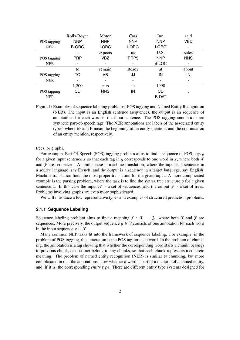
Figure 1: Examples of sequence labeling problems: POS tagging and Named Entity Recognition(NER). The input is an English sentence (sequence), the output is an sequence ofannotations for each word in the input sentence. The POS tagging annotations aresyntactic part-of-speech tags. The NER annotations are labels of the associated entitytypes, where B- and I- mean the beginning of an entity mention, and the continuationof an entity mention, respectively.

trees, or graphs.For example, Part-Of-Speech (POS) tagging problem aims to find a sequence of POS tags y

for a given input sentence x so that each tag in y corresponds to one word in x, where both Xand Y are sequences. A similar case is machine translation, where the input is a sentence ina source language, say French, and the output is a sentence in a target language, say English.Machine translation finds the most proper translation for the given input. A more complicatedexample is the parsing problem, where the task is to find the syntax tree structure y for a givensentence x. In this case the input X is a set of sequences, and the output Y is a set of trees.Problems involving graphs are even more sophisticated.

We will introduce a few representative types and examples of structured prediction problems.

2.1.1 Sequence Labeling

Sequence labeling problem aims to find a mapping f : X → Y , where both X and Y aresequences. More precisely, the output sequence y ∈ Y consists of one annotation for each wordin the input sequence x ∈ X .

Many common NLP tasks fit into the framework of sequence labeling. For example, in theproblem of POS tagging, the annotation is the POS tag for each word. In the problem of chunk-ing, the annotation is a tag showing that whether the corresponding word starts a chunk, belongsto previous chunk, or does not belong to any chunks, so that each chunk represents a concretemeaning. The problem of named entity recognition (NER) is similar to chunking, but morecomplicated in that the annotations show whether a word is part of a mention of a named entity,and, if it is, the corresponding entity type. There are different entity type systems designed for

2

S

.

.

VP

PP

NP

NN

mat

DT

the

IN

on

VBD

sat

NP

NN

cat

DT

The

The cat sat on the mat

root

Figure 2: Examples of parsing problem. Left: constituent parsing. Right: unlabeled dependencyparsing.

different tasks. In a very simple case, the entity types may consist of person (PER), location(LOC) organization (ORG), and date (DAT).

We show two examples of sequence labeling problems, POS tagging and NER, in Figure 1.For the POS tags used in the annotation, we use the tag set from Penn Treebank (Marcus et al.,1993). For NER, we use tags B-ORG, B-LOC, and B-DAT to denote the beginning of mentionsof organization “Rolls-Royce Motor Cars Inc.”, location “U.S.”, and date “1990”, respectively;we use tag I-ORG to denote the continuation of previous organization mention.

2.1.2 Parsing

Parsing takes a sentence, i.e., a sequence, as input and outputs a tree structure.The most common syntactic parsing, constituent parsing, parses a sentence to a syntax tree

following a given context-free grammar. An exemplary grammar is:

S→ NP VPVP→ VB PPNP→ DT NN. . .NN→ catVB→ sit. . .

Constituent parsing is one of the most important core NLP tasks since its outputs are very use-ful in linguistic analysis. There are various parsing similar to constituent parsing, but definedfor different grammars, such as tree-adjoining grammar (Joshi et al., 1975), and combinatorycategorial grammar (Altmann and Steedman, 1988).

Another type of parsing different from previous parsing methods where the parsing rules, i.e.,the grammar, is not explicitly defined is dependency parsing. In dependency parsing, the tree

3

edges directs from a tail word to a head word, indicating that the head word depends on the tailword. One word can only depend on one other word, while one word can be the dependents ofmany other words.

Figure 2 shows examples of syntax parsing and dependency parsing for sentence “The cat saton the mat.”.

Both constituent parsing and dependency parsing are defined in the syntactic domain. For se-mantic domain, semantic parsing parses sentences to semantic representations. There are severalkinds of popular semantic representations such as logical expression (Tang and Mooney, 2001),lambda expression (Zettlemoyer and Collins, 2005), lambda Dependency-based CompositionalSemantics (DCS) (Berant et al., 2013; Liang, 2013).

Here is an example of semantic parsing in the meaning representation of lambda expression:

input What is the capital of the largest state by area?output (capital (argmax state size))

2.1.3 Machine Translation

Machine translation converts a sentence in a source language to a sentence in a target language,keeping the meaning unchanged. Different from sequence labeling problem, there is no one-to-one mapping between the words in the source language and the target language.

Here is a translation example taken from (Mi et al., 2008) that will be used in Section 4.

ChineseBushı yu Shalong juxıng le huıtanBush with Sharon hold -ed meeting

English Bush held a meeting with Sharon

Despite its simple problem definition, machine translation is a very complicated task, sincefundamentally translation is a process involving both syntax and semantics. However, mostcurrent approaches focus on the syntax level, as semantic analysis is still not mature yet.

2.2 Formalization

For simplicity we use the sequence labeling problem as an example to establish the mathematicalformalization. This formalization will be used in the following sections to demonstrate learningand decoding algorithms for structured prediction problems.

In the sequence labeling problem, the input

x = (x1x2 . . . xm) ∈ X

is a sequence of length m, which is typically a sentence in some language, say English. Theoutput

y = (y1y2 . . . ym) ∈ Y

is a sequence of the same length, where yi is an annotation for word xi. Usually we use Y(x) ∈Y to denote the set of all possible annotation sequences for input x.

There are two typical problems for structured prediction.

4

Inference Problem

The inference problem finds the best output y for a given input x, under some scoring functionF : X × Y → R:

y? = arg maxy∈Y(x)

F (x, y).

This problem is actually harder than it appears to be. As the output y = (y1y2 . . . ym) isa sequence of m tags, assume the tags belong to a set of all possible tags T : ∀i, yi ∈ T . Abrute-force search will take O(|T |m) time, which is not affordable even for relatively small m.

The goal of inference problem is to find an efficient algorithm to find the best output withinthe time limit.

Sometimes the inference problem is also called the decoding problem.

Learning Problem

The learning problem aims to find the best scoring function F for any given pairs of input andoutput (x, y), under some extrinsic measurement.

However, to measure the quality of the scoring function is not trivial. In fact, there can bemany different measurements. For some tasks like sequence labeling, the label accuracy is usedas the measurement. For some tasks like machine translation, complicated measurements likeBLEU (Papineni et al., 2002) are invented.

Different measurements result in different learning methods, since the goal of learning is tooptimize F to maximize the predication quality under the given measurement.

2.3 Structured Prediction from Machine Learning Perspective

Machine learning methods, or more specifically, statistical methods, dominate the learning forstructured prediction problems.

2.3.1 Supervised vs. Unsupervised

In supervised learning framework, we are given a set of training corpus

{(x(1), y(1)), (x(2), y(2)), . . . , (x(N), y(N))} ⊂ X × Y

that contains N training input/output pairs.The goal is to find the scoring function F (the learning problem), and we need to make sure

that it is efficient enough to use F to find the best output y for a given x (the inference problem).Learning can also be unsupervised where we only have input but not the output. Unsuper-

vised learning is very useful, especially for large dataset, because for supervised learning, weneed manually annotated output y as the target to learn, which is not always available, especiallyfor large datasets, or for rare languages, while the annotations are not necessary for unsupervisedlearning.

As a middle ground between supervised learning and unsupervised learning, there is alsosemi-supervised learning, where we use the learning results from supervised learning on a

5

small manually annotated dataset as seeds, and do unsupervised learning on the large datasetto improve the accuracy.

Here we only consider supervised learning in the following sections, because it is simpler,and is the base for many unsupervised and semi-supervised methods.

2.3.2 Generative vs. Discriminative

There are two ways to model the scoring function.In the first one, we want the scoring function F to give a score for every input/output pair

(x, y), i.e., F scores x and y jointly. In this case, F is of the form F (x, y). We call thiskind of models generative models, because in the probabilistic perspective, F is similar to thegenerative probability of pair (x, y), P (x, y).

In the second one, note that we only need to pick the best output y for each given x, and thereis no need to compare the scores of two pairs of input/output. In this case, F can be modeled asa function of form Fx(y), i.e., x is a hyper-parameter of the scoring function. In the probabilisticframework, F can be written as P (y|x). We call this kind of models discriminative models.

Both generative and discriminative models are widely used to solve structured predictionproblems. However, since we focus on a discriminative model, perceptron, the following sec-tions mostly discuss only discriminative model.

3 Structured Perceptron

As the simplest machine learning algorithm, perceptron is adapted to handle structured predic-tion problems (Collins, 2002). In this section we first introduce the generic perceptron (Rosen-blatt, 1957) and its convergence proof. After that we show the perceptron that handles structuredprediction problems, the adapted convergence proof, and how this affects the training process.

3.1 Generic Perceptron and its Convergence

Generic perceptron (Rosenblatt, 1957) is a binary classifier based on a linear prediction function.More formally, the prediction function is:

f(x) =

{1 if w · x > b

0 otherwise,

where the input x is a vector of numbers, the output y is a binary number, parameter w is theweight vector, and b is the bias. However, to simplify the representation, a widely used techniqueis to augment the input vector x by appending a value 1 at the end,

x = (x1, x2, . . . , xm, 1)

6

Algorithm 1 Learning algorithm for generic perceptron.

1: Input: training set D = {(x(1), y(1)), (x(2), y(2)), . . . , (x(N), y(N)} ∈ X × Y , number ofiterations I

2: Output: weight vector w3: w← (0, 0, . . . , 0)4: for i = 1, . . . , I do5: for j = 1, . . . , N do6: if y(j)x(j) ·w ≤ 0 then7: w← w + y(j)x(j)

return w

and drop the bias b. The prediction function is then simplified as

f(x) =

{1 if w · x > 0

0 otherwise,

In the training (Algorithm 1), perceptron learns the weight vector w in an online fashion. Itprocesses examples in the training set one after another. For each example, perceptron checksif it can be classified correctly. If not, perceptron will update the weight vector by moving wtowards the current input vector.

It has been proven that, for a linear separable training set, perceptron will eventually reach aweight vector w that correctly classifies each example (Rosenblatt, 1957). This proof is closelyrelated to perceptron’s adaptation for structured classification, and, thus, is described here.

Denote R to be maximal radius of training examples: R = maxi‖x(i)‖. Assume the trainingset D is separable by a unit oracle vector u with optimal margin

γ = maxu:‖u‖=1

min(x,y)∈D

yx · u.

Theorem 1 (convergence of binary perceptron). For a separable datasetD = {x(i), y(i)}Ni withoptimal margin γ and radius R, perceptron terminates after t updates, where t ≤ R2

γ2.

Proof. Let wt be the weight vector before the tth update. Suppose tth update occurs on example(xt, yt). Following properties hold:

1. yt(u · xt) ≥ γ (margin on unit vector)

2. yt(wt · xt) ≤ 0 (Algorithm 1 Line 6)

3. ‖xt‖2 ≤ R2 (radius)

The update formula can be rewritten as:

wt+1 = wt + ytxt. (1)

‖wt+1‖ is bounded in two directions.

7

1. Dot product both sides of Equation 1 with oracle vector u:

u ·wt+1 = u ·wt + yt(u · xt)≥ u ·wt + γ (margin)

≥∑t

γ = tγ (by induction)

2. Take the norm of both sides of Equation 1:

‖wt+1‖2 =‖wt + ytxt‖2

=‖wt‖2 + ‖ytxt‖2 + 2ytwt · xt

≤‖wt‖2 + ‖xt‖2 (Property 2)

≤‖wt‖2 +R2 (radius)

=∑t

R2 = tR2 (by induction)

Combining the two bounds for wt+1 leads to:

t2γ2 ≤ ‖wt+1‖2 ≤ tR2,

which indicates t ≤ R2

γ2.

With this convergence proof, a generic perceptron will eventually correctly classify everyexample in a linear separable training set. However, this usually means that this perceptron istrained specially for the training set, but does not generalize well on development and testingdatasets.

(Freund and Schapire, 1999) introduce averaged perceptron that assigns more weights forthe examples learned at the beginning of the training, which is called weight averaging. Withweight averaging, perceptron achieves some kind of large margin effect, i.e., it maximizes theseparating margin for a given training set, which is the essential idea of Support Vector Machine(SVM) and generalizes well for unseen datasets. However, the original algorithm of averagedperceptron (Freund and Schapire, 1999) requires significant amount of computation for weightaveraging. In (Daume, 2006), an improved version of averaged perceptron is introduced. Thisimprovement significantly reduces the extra computation for weight averaging. (Algorithm 2)

Binary perceptron can be further extended to handle multiclass classification. In multiclassclassification setting, for each input x, the corresponding output y belongs to a finite set Y . Thefeature function Φ(x, y) maps the pair (x, y) to a vector of real numbers. Multiclass perceptronassigns an input x an output y by:

y = argmaxy′∈Y

Φ(x, y′) ·w

The convergence property still holds for multiclass perceptron. Due to its similarity to thebinary case, the proof is not contained in this survey.

8

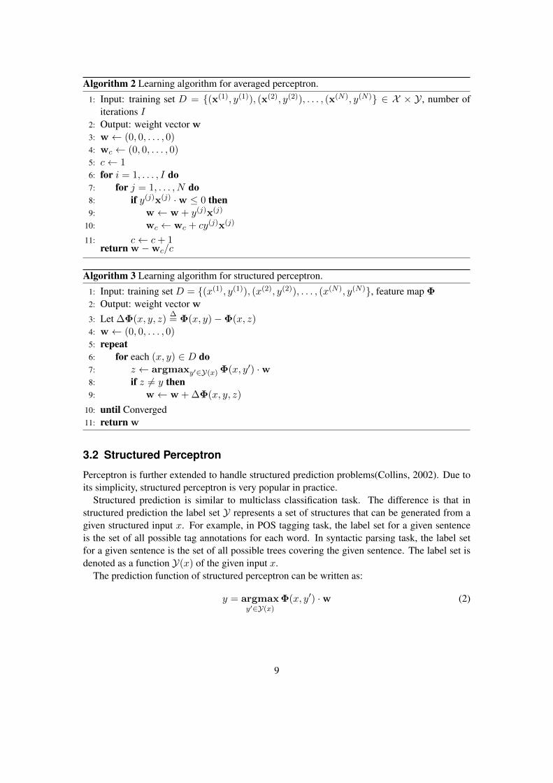
Algorithm 2 Learning algorithm for averaged perceptron.

1: Input: training set D = {(x(1), y(1)), (x(2), y(2)), . . . , (x(N), y(N)} ∈ X × Y , number ofiterations I

2: Output: weight vector w3: w← (0, 0, . . . , 0)4: wc ← (0, 0, . . . , 0)5: c← 16: for i = 1, . . . , I do7: for j = 1, . . . , N do8: if y(j)x(j) ·w ≤ 0 then9: w← w + y(j)x(j)

10: wc ← wc + cy(j)x(j)

11: c← c+ 1return w −wc/c

Algorithm 3 Learning algorithm for structured perceptron.

1: Input: training set D = {(x(1), y(1)), (x(2), y(2)), . . . , (x(N), y(N)}, feature map Φ2: Output: weight vector w

3: Let ∆Φ(x, y, z)∆= Φ(x, y)−Φ(x, z)

4: w← (0, 0, . . . , 0)5: repeat6: for each (x, y) ∈ D do7: z ← argmaxy′∈Y(x) Φ(x, y′) ·w8: if z 6= y then9: w← w + ∆Φ(x, y, z)

10: until Converged11: return w

3.2 Structured Perceptron

Perceptron is further extended to handle structured prediction problems(Collins, 2002). Due toits simplicity, structured perceptron is very popular in practice.

Structured prediction is similar to multiclass classification task. The difference is that instructured prediction the label set Y represents a set of structures that can be generated from agiven structured input x. For example, in POS tagging task, the label set for a given sentenceis the set of all possible tag annotations for each word. In syntactic parsing task, the label setfor a given sentence is the set of all possible trees covering the given sentence. The label set isdenoted as a function Y(x) of the given input x.

The prediction function of structured perceptron can be written as:

y = argmaxy′∈Y(x)

Φ(x, y′) ·w (2)

9

The learning algorithm for structured perceptron is shown in Algorithm 3.As discussed in Section 2, the major problem in structured prediction is that the size of setY(x) grows exponentially with the size of input x, which means that to precisely enumerateover all possible label set Y(x) in Equation 2 to find the candidate with the highest score, isimpossible due to time constraints during the decoding. Furthermore, most modern tasks requireto train the structured perceptron over a huge training set. For example, the Penn Treebank(Marcus et al., 1993) for syntactic parsing task consists of ∼ 40, 000 sentences. This makes anefficient inference algorithm crucial for structured prediction problems.

3.3 Inference Problem

Vast efforts have been made in improving the efficiency of searching for the structure with themaximal score in structured inference. In general, these approaches can be classified as twodifferent categories: exact search and inexact search. These two approaches are orthogonal,which means that they are usually combined to make the search fast.

3.3.1 Exact Inference: Dynamic Programming

Exact inference relies on the properties of many structured prediction tasks that the scoringfunction F (x, y) = Φ(x, y) ·w can be defined to be decomposable.

Take POS tagging task as an example, the input x is a sequence of words, (x1, x2, . . . , xm),and the output y is a sequence of POS tags, (y1, y2, . . . , ym).

Denote the set of all possible POS tags as T . There are |T |m possible POS tags annotationsto enumerate for the argmax operation during decoding input x.

A decomposable scoring function for POS tagging task can be defined to be the sum of step-wise tagging results. More specially, the stepwise scoring function for predicting current POStag yi can only rely on yi, k previous POS tags yi−k, . . . , yi−1, and the fixed given input sentencex.

F (x, y) =

m∑i=1

F (x, yi−k, yi−k+1, . . . , yi)

Here to simplify the notation, the POS tags for yi, i ≤ 0 are defined as a special tag, “beginningof sentence”, 〈s〉.

For structured perceptron, the scoring function F (x, y) = Φ(x, y) ·w can be decomposed as

F (x, y) =m∑i=1

Φ(x, yi−k, yi−k+1, . . . , yi) ·w,

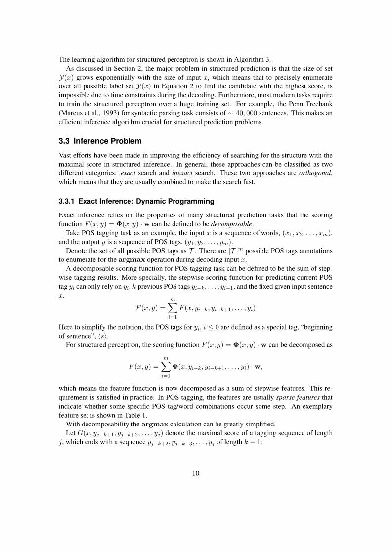
which means the feature function is now decomposed as a sum of stepwise features. This re-quirement is satisfied in practice. In POS tagging, the features are usually sparse features thatindicate whether some specific POS tag/word combinations occur some step. An exemplaryfeature set is shown in Table 1.

With decomposability the argmax calculation can be greatly simplified.Let G(x, yj−k+1, yj−k+2, . . . , yj) denote the maximal score of a tagging sequence of length

j, which ends with a sequence yj−k+2, yj−k+3, . . . , yj of length k − 1:

10

atomic featuresxi−2, xi−1, xi, xi+1, xi+2, xi−2,yi−2, yi−1, yi

combined features

yi−2|yi−1|yi, yi−1|yi,xi−2|yi, xi−1|yi, xi|yi, xi+1|yi, xi+2|yi, xi−2|yi,xi−2|yi−1|yi, xi−1|yi−1|yi, xi|yi−1|yi,xi+1|yi−1|yi, xi+2|yi−1|yi, xi−2|yi−1|yi

Table 1: An exemplary feature set for POS tagging task.

G(x, yj−k+2, yj−k+3, . . . , yj) = maxy1,y2,...,yj−k+1

i∑j=1

F (x, yj−k, yj−k+1, . . . , yj)

= maxyj−k+1

G(x, yj−k+1, yj−k+2, . . . , yj−1)

+ F (x, yj−k+1, yj−k+2, . . . , yj)

maxy∈Y(x)

F (x, y) = maxy∈Y(x)

m∑i=1

F (x, yi−k, yi−k+1, . . . , yi)

= maxy∈Y(x)

G(x, ym−k+2, ym−k+3, . . . , ym)

= maxym−k+2,ym−k+3,...,ym

G(x, ym−k+2, ym−k+3, . . . , ym)

= maxym−k+1,ym−k+2,...,ym

G(x, ym−k+1, ym−k+2, . . . , ym−1)

+ F (x, ym−k+1, ym−k+2, . . . , ym)

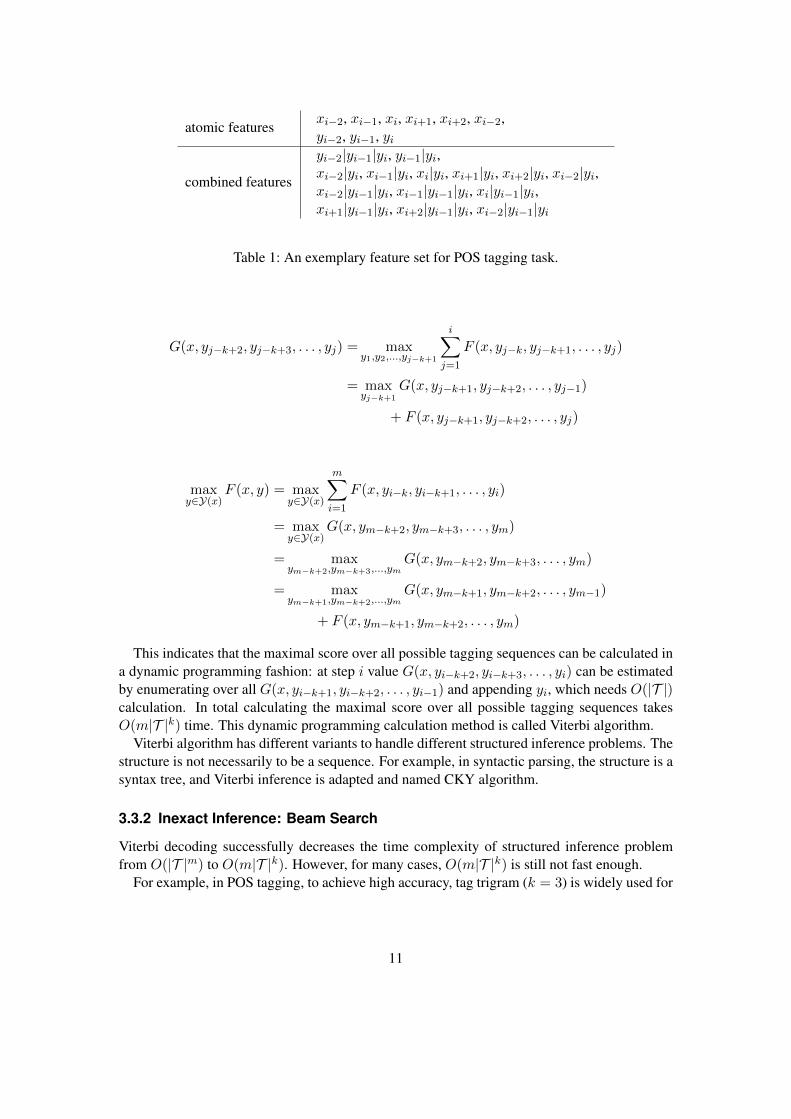
This indicates that the maximal score over all possible tagging sequences can be calculated ina dynamic programming fashion: at step i value G(x, yi−k+2, yi−k+3, . . . , yi) can be estimatedby enumerating over all G(x, yi−k+1, yi−k+2, . . . , yi−1) and appending yi, which needs O(|T |)calculation. In total calculating the maximal score over all possible tagging sequences takesO(m|T |k) time. This dynamic programming calculation method is called Viterbi algorithm.

Viterbi algorithm has different variants to handle different structured inference problems. Thestructure is not necessarily to be a sequence. For example, in syntactic parsing, the structure is asyntax tree, and Viterbi inference is adapted and named CKY algorithm.

3.3.2 Inexact Inference: Beam Search

Viterbi decoding successfully decreases the time complexity of structured inference problemfrom O(|T |m) to O(m|T |k). However, for many cases, O(m|T |k) is still not fast enough.

For example, in POS tagging, to achieve high accuracy, tag trigram (k = 3) is widely used for

11

Dataset D = {(x, y)}x fruit flies fly .y N N V .

Search sapce Y(x) = {N} × {N, V} × {N, V} × {.}Features Φ(x, y) = (#N→N (y),#V→.(y))Training process:

iter label z ∆Φ(x, y, z) ∆Φ ·w new w

0 (0, 0)1 N N N . (−1,+1) 0 (−1, 1)2 N V N . (+1,+1) 0 (0, 2)3 N N N . (−1,+1) 2 (−1, 3)4 N V N . (+1,+1) 2 (0, 4)

... infinite loop ...

Figure 3: A POS tagging example where standard structured perceptron does not converge.The dataset only contains one sentence “fruit flies fly.”. The simplified tagging setT = {N,V, .}. The simplified feature function only counts the number of “N-N” tagbigrams (#N→N (y)), and the number of “V-.” tag bigrams (#V→.(y)). The Viterbidecoding algorithm is greedy, i.e., beam size b = 1. (Huang et al., 2012)

decoding. A typical tag set like the Penn Treebank contains T = 36 tags. Enumerating over allpossible candidate tag for each G value is still very time-consuming.

Thus approximation, i.e., inexact search, is used to further accelerate the decoding. The mostwidely used inexact search is beam search. In beam search, at each step, only top b values of Gare kept and further extended. Beam search decreases the time complexity to O(mb), which isusually sufficiently fast for most decoding problems.

3.4 Convergence of Structured Perceptron

For the learning problem, at first glance, the convergence property for structured perceptronseems exactly the same as multiclass perceptron, since structured perceptron is similar to anextension of multiclass perceptron with infinite number of classes.

However, as the example in Figure 3 shows, a simple combination of structured perceptronwith inexact search, i.e., beam search, is problematic. This example shows that structured per-ceptron on very short sentences and simple features are not guaranteed to converge.

3.5 Violation-Fixing Perceptron

The first approach to address this convergence problem is in (Collins and Roark, 2004). In thiswork, a new kind of perceptron, called “incremental perceptron” by (Daume, 2006), is proposed.

The key intuition in (Collins and Roark, 2004) is that during beam search, at some step thepartially finished reference output y ranks too low and falls out of the beam, this is obviouslywrong since the reference should always stay in the beam and rank first at the last step of thebeam. To fix this mistake, the perceptron update should occur at the very step where the partial

12

early

max

-vi

olat

ion

late

st

full

(sta

ndar

d)

best in the beam

worst in the beamfalls off

the beam biggestviolation

last valid update

correct sequence

invalidupdate!

Figure 4: Update methods in structured perceptron with beam search.

reference output falls out of the beam, against the top ranked candidate. This strategy is calledearly update. (See Figure 4 “early” update.)

The major problem about early update is that the learning takes long time. This is reasonablesince, as shown in Figure 4, the update is mostly done for a short prefix of a tagging sequence.The structured perceptron is trained to be familiar with the prefix of a sentence, but is very error-prone for the reset of the sentence where it has never seen before. It could only see the wholesentence after many iterations so that it fixes every errors before the end, one per iteration.

Another problem remains is the theoretical reason that explains the effectiveness of earlyupdate, or the ineffectiveness of standard update.

Both of these two problems are addressed in (Huang et al., 2012), where the convergenceproof for structured perceptron is reexamined. This proof is conceptually the same as the binarycase, but extended to the specially case in the incremental setting where the update is on theprefixes of a sequence.

First, in the incremental setting, the training setD is actually consists of prefixes of sequences,since the update can occur on any prefix of a given sequence.

Assume the training setD is separable by feature map Φ and unit oracle vector u with optimalmargin

γ = maxu:‖u‖=1

min(x,y)∈D,z 6=y

u ·∆Φ(x, y, z).

Let R = max(x,y)∈D,z 6=y ∆Φ(x, y, z) be the radius.

Theorem 2 (convergence of structured perceptron). For a separable dataset D = {x(i), y(i)}Niwith optimal margin γ and radius R under feature map Φ, structured perceptron terminatesafter t updates, where t ≤ R2

γ2.

Proof. Let wt be the weight vector before the tth update. Suppose tth update occurs on example(xt, yt), and the top candidate z 6= yt.

Following properties hold:

1. u ·∆Φ(xt, yt, z) ≥ γ (margin on unit vector)

13

2. ∆Φ(xt, yt, z) < 0 (Algorithm 3 Line 7)

3. ‖∆Φ(xt, yt, z)‖2 ≤ R2 (radius)

The update formula is:wt+1 = wt + ∆Φ(xt, yt, z) (3)

‖wt+1‖ is bounded in two directions.

1. Dot product both sides of Equation 3 with oracle vector u:

u ·wt+1 = u ·wt + u ·∆Φ(xt, yt, z)

≥ u ·wt + γ (margin)

≥∑t

γ = tγ (by induction)

2. Take the norm of both sides of Equation 3:

‖wt+1‖2 =‖wt + ∆Φ(xt, yt, z)‖2

=‖wt‖2 + ‖∆Φ(xt, yt, z)‖2 + 2wt ·∆Φ(xt, yt, z)

≤‖wt‖2 + ‖∆Φ(xt, yt, z)‖2 (Property 2)

≤‖wt‖2 +R2 (radius)

=∑t

R2 = tR2 (by induction)

Combining the two bounds for wt+1 leads to:

t2γ2 ≤ ‖wt+1‖2 ≤ tR2,

which indicates t ≤ R2

γ2.

To theoretically explain why standard perceptron does not always converge with beam search,note that Property 2 in the above proof, which is called “violation” in (Huang et al., 2012), isrequired in the second part of the proof. However, this is not necessarily always true. As shownin Figure 3, ∆Φ ·w is positive for some updates, which violates the convergence property.

Furthermore, this observation points out that, as long as the update satisfies the violationproperty, the convergence property holds.

For early update, since at the step where the reference falls out of the beam, the referencecandidate y ranks lower than the top candidate z:

Φ(x, y) ·w ≤ Φ(x, z) ·w⇒ ∆Φ(x, y, z) ·w ≤ 0.

Thus, the convergence is still guaranteed.This observation further points out a new update strategy, “max-violation” update, which

updates at the step where the score difference between the partial reference candidate and the

14

input: w0 . . . wn−1

axiom 0 : 〈0, ε〉: ∅

SHIFT` : 〈j, S〉 : A

`+ 1 : 〈j + 1, S|wj〉 : Aj < n

LEFT-REDUCE` : 〈j, S|s1|s0〉 : A

`+ 1 : 〈j, S|s0〉 : A ∪ {s1xs0}

RIGHT-REDUCE` : 〈j, S|s1|s0〉 : A

`+ 1 : 〈j, S|s1〉 : A ∪ {s1ys0}

goal 2n− 1 : 〈n, s0〉: A

Figure 5: An abstraction of the arc-standard deductive system.

top candidate in the beam is maximal (Figure 4). The intuition behind this is that at such step thestructured perceptron can learn most, and, thus, converges faster. However, there is no theoreticalproof for the convergence of max-violation update.

3.6 Applications

Besides POS tagging, structured perceptron has been extended to solve various structured pre-diction problems, and to handle different structures.

3.6.1 Incremental Dependency Parsing

As mentioned in Section 2, dependency parsers converts an input sentence to a dependency tree.There are two popular parsing algorithms for dependency parsing. The minimum-spanning treealgorithm (McDonald et al., 2005) first assigns a penalty to the potential edges between eachpair of words, and then finds a minimum-spanning tree as the dependency tree. The incrementalparsing (Nivre, 2003) converts the tree construction process into a sequence of transition actions.

More specially, for standard incremental dependency parser (which is called “arc-standard”by Nivre), the parsing states are composed of a stack, a buffer, and an arc set. Parsing transitionsare applied to states to generate new states. There are three kinds of transitions: SHIFT, LEFT-REDUCE, and RIGHT-REDUCE, which are summarized in Figure 5. The SHIFT transition popsthe top word from the buffer and pushes it onto the stack. The LEFT-REDUCE transition popsthe top two items, s0 and s1, from the stack, and add an dependency relation s1

xs0 into the arc-set. The RIGHT-REDUCE transition is similar, except that the dependency relation is s1

ys0. Anexemplary parsing sequence for sentence “The cat sat on the mat” to generate the dependencytree in Figure 2 Right is shown in Table 2.

For dependency parsing, although the desired output should be a tree, the incremental parsingtask converts it to a sequence of actions, which makes the task very similar to the POS tagging

15

step action stack buffer arc added0 - root The cat . . .1 SHIFT root The cat sat . . .2 SHIFT root The cat sat on . . .3 LEFT-REDUCE root cat sat on . . . Thexcat4 SHIFT root cat sat on the . . .5 LEFT-REDUCE root sat on the . . . catxsat6 SHIFT root sat on the mat7 RIGHT-REDUCE root sat the mat satyon8 SHIFT root sat the mat9 SHIFT root sat the mat10 LEFT-REDUCE root sat mat thexmat11 RIGHT-REDUCE root sat satymat12 RIGHT-REDUCE root rootysat

Table 2: Incremental dependency parsing transitions for sentence “The cat sat on the mat” togenerate the dependency tree in Figure 2 Right.

task. However, this conversion is not perfect: there can be more than one correct action se-quences that lead to the same reference dependency tree. For example, the action at step 5 inTable 2 can be delayed to be performed after step 11, and the output dependency tree keeps thesame. This is call spurious ambiguity. In practice, for incremental parsing a widely used strategyit to greedily choose one correct action sequence as the reference sequence, and train the percep-tron to update towards this chosen reference. This strategy works well for dependency parsing,since the number of correct sequences are not big. But for some other tasks, this strategy is notenough. More details about this will be discussed in Section 4.

3.6.2 Syntactic Parsing with Forest

The syntactic parsing, or constituency parsing, parses an input sentence into a syntax tree.The most widely used syntactic parsing algorithm is the bottom-up CKY parsing. This pro-

cess can be formulated this as approximated bottom-up inference that can compactly representexponentially many outputs trees using hypergraph representation, i.e., forests (Klein and Man-ning, 2005; Huang, 2008).

In the parsing with forest setting, a parsing rule is interpreted as a hyperedge connecting theterminal/non-terminals on the right side of the rule to the non-terminals on the left side. TheViterbi algorithm is also adapted to hypergraph setting to solve the decoding problem.

More formally, the input of constituency parsing with hypergraphs is a sentence, and theoutput is a more complicated and general structure: a hypergraph. (Zhang et al., 2013) extendstructured perceptron to handle the inexact search over hypergraphs. Figure 6 from (Zhang et al.,2013) shows a hypergraph containing both the reference subtree (bold lines) and the Viterbi sub-tree (dashed lines). Different from the POS tagging task where there is a linear beam, in the

16

Figure 6: A parsing hypergraph showing the union of the reference (bold) and Viterbi (dashed)subtrees. (Zhang et al., 2013)

hypergraph parsing, the beam is organized following a topological order. The early update strat-egy and max-violation update strategy both can be adapted to work on the topological order. Forthe early update, the structured perceptron will update at the lowest hypernode where the refer-ence hyperedge falls out of the beam. For the max-violation update, the structured perceptronwill update at the hypernode where the score difference between the reference hyperedge andthe Viterbi hyperedge is maximum.

3.7 Discussion: CRF vs. Structured Perceptron

Conditional Random Field (CRF) (Lafferty et al., 2001) is another very popular discriminativeclassifier for structured prediction problems. It is very similar to structured perceptron in thatboth of them optimize over a global objective function, unlike other classifiers, e.g., maximumentropy models, that only optimize over a local objective function.

More formally, CRF can be viewed as a structured extension of maximum entropy models. Itassumes the same feature function Φ as structured perceptron, and models the probability of angiven output as:

p(y|x) =1

Z(x)exp[w ·Φ(x, y)]

Z(x) =∑

y′∈Y(x)

exp[w ·Φ(x, y′)]

Here, Z(x) is called partition function, which needs to sum over all incorrect outputs. Com-puting Z(x) is very time-consuming in general. If the feature function Φ is required to satisfy

17

the same property as in structured perceptron, Z(x) can be computed fast enough using dynamicprogramming techniques (Lafferty et al., 2001; Sutton and McCallum, 2010). This requirementis satisfied for most structured prediction problems.

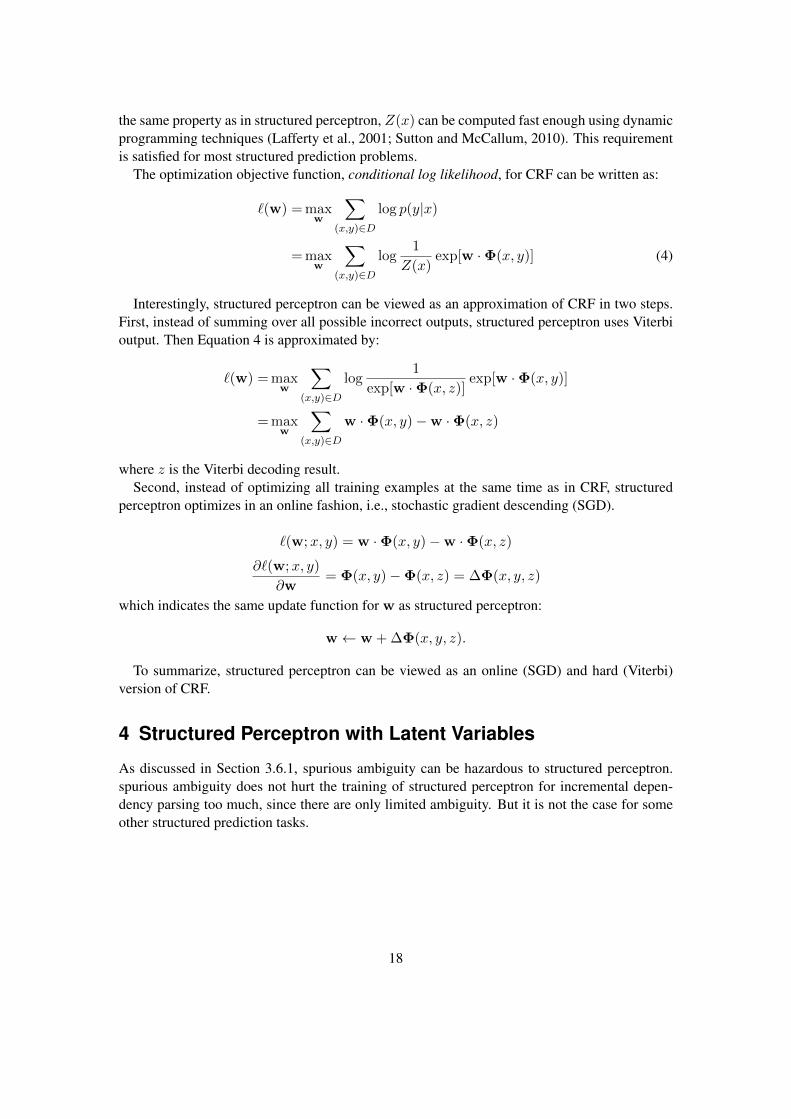
The optimization objective function, conditional log likelihood, for CRF can be written as:

`(w) = maxw

∑(x,y)∈D

log p(y|x)

= maxw

∑(x,y)∈D

log1

Z(x)exp[w ·Φ(x, y)] (4)

Interestingly, structured perceptron can be viewed as an approximation of CRF in two steps.First, instead of summing over all possible incorrect outputs, structured perceptron uses Viterbioutput. Then Equation 4 is approximated by:

`(w) = maxw

∑(x,y)∈D

log1

exp[w ·Φ(x, z)]exp[w ·Φ(x, y)]

= maxw

∑(x,y)∈D

w ·Φ(x, y)−w ·Φ(x, z)

where z is the Viterbi decoding result.Second, instead of optimizing all training examples at the same time as in CRF, structured

perceptron optimizes in an online fashion, i.e., stochastic gradient descending (SGD).

`(w;x, y) = w ·Φ(x, y)−w ·Φ(x, z)

∂`(w;x, y)

∂w= Φ(x, y)−Φ(x, z) = ∆Φ(x, y, z)

which indicates the same update function for w as structured perceptron:

w← w + ∆Φ(x, y, z).

To summarize, structured perceptron can be viewed as an online (SGD) and hard (Viterbi)version of CRF.

4 Structured Perceptron with Latent Variables

As discussed in Section 3.6.1, spurious ambiguity can be hazardous to structured perceptron.spurious ambiguity does not hurt the training of structured perceptron for incremental depen-dency parsing too much, since there are only limited ambiguity. But it is not the case for someother structured prediction tasks.

18

4.1 POS Tagging with Latent Variables

The previous POS tagging task is simple that for every sentence x, the gold reference y is knownin the training set. In other words, there is no spurious ambiguity in the training.

However, some people claim that the given tag set T might not be specific enough. Thisis a quite reasonable thought especially for some languages with relatively low resources, e.g.,Chinese Treebank (CTB) (Xue et al., 2005).

An approach to address this problem is to introduce latent tags. For example, tag NN canbe split into two different tags NN1 and NN2 where the former is for countable noun while thelatter is for uncountable noun. Following this intuition, we introduce the latent tags like NN1

and NN2 that will be our training target. In evaluation of tagging accuracy, both NN1 and NN2

are converted back to NN.More formally, for a given tag set T , there is a mapping function H that maps each item yi inT to a latent label set H(yi) = {hyi,1hyi,2, . . . , hyi,k}. For a given sentence x = (x1x2 . . . xm),and a given reference tag sequence y = (y1y2 . . . ym), the associated latent tag sequence ish = (h1h2 . . . hm) such that hi ∈ H(yi), 1 ≤ i ≤ m.

During the training, h is the latent variable since it is always unknown. Structured perceptronis adapted to handle this latent variable.

The Viterbi decoding result is

z = argmaxh′

Φ(x, h′) ·w

The best latent tag sequence that is consistent with the given reference y is:

h = argmaxh′∈H(y)

Φ(x, h′) ·w

The update function is:w← w + ∆Φ(x, h, z)

4.2 Convergence of Latent Variable Perceptron

(Sun et al., 2009) give a convergence proof for structured perceptron with latent variables similarto the POS tagging task. This convergence proof guarantees that, if the latent variables arethe latent tags that are split from reference tags, and the structured perceptron for the originalproblem converges, then the new latent variable structured perceptron also converges.

The key intuition for this proof is to show that a new separation margin γ for the featurefunction over the latent tags can be induced from the separation margin γ in the original proof.

More formally, note that the original separation margin is defined as

γ = maxu:‖u‖=1

min(x,y)∈D,z 6=y

u ·∆Φ(x, y, z).

The new separation margin over latent tags is:

γ = maxu:‖u‖=1

min(x,y)∈D,h∈H(y),z 6∈H(y)

u ·∆Φ(x, h, z).

19

In addition, note that in the above equation Φ is used over h, which is not defined actually.The new feature function Φ is actually “augmented” from the old feature space to the new latentspace. A feature fi that uses unigram tag yi is mapped to a new set of possible features usinghyi,1, hyi,2, . . . , hyi,ki , where ki = |H(yi)|. Similarly feature fj that uses bigram tags yj , y′j ismapped to a new set of possible features of size kj = |H(yj)||H(y′j)|. For an original featurefunction Φ with n features, the dimension augmentation of the feature space can be denoted as(k1, k2, . . . , kn) where n is the size of the original feature space size.

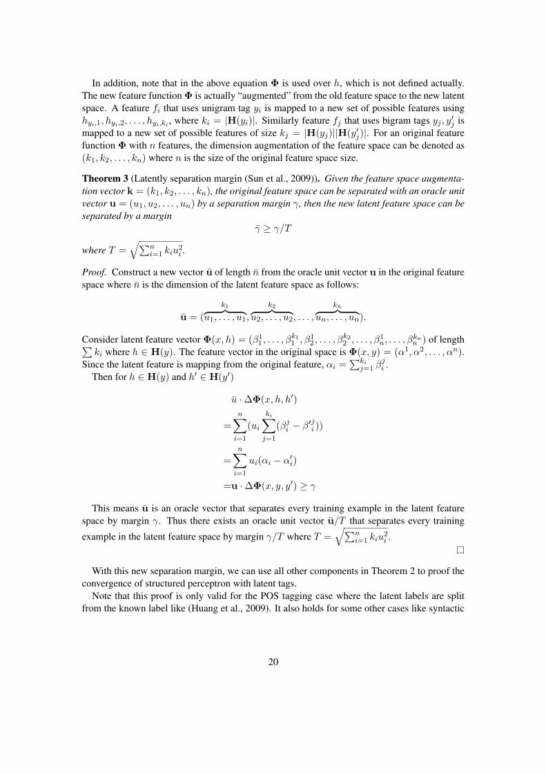
Theorem 3 (Latently separation margin (Sun et al., 2009)). Given the feature space augmenta-tion vector k = (k1, k2, . . . , kn), the original feature space can be separated with an oracle unitvector u = (u1, u2, . . . , un) by a separation margin γ, then the new latent feature space can beseparated by a margin

γ ≥ γ/T

where T =√∑n

i=1 kiu2i .

Proof. Construct a new vector u of length n from the oracle unit vector u in the original featurespace where n is the dimension of the latent feature space as follows:

u = (

k1︷ ︸︸ ︷u1, . . . , u1,

k2︷ ︸︸ ︷u2, . . . , u2, . . . ,

kn︷ ︸︸ ︷un, . . . , un).

Consider latent feature vector Φ(x, h) = (β11 , . . . , β

k11 , β1

2 , . . . , βk22 , . . . , β1

n, . . . , βknn ) of length∑

ki where h ∈ H(y). The feature vector in the original space is Φ(x, y) = (α1, α2, . . . , αn).Since the latent feature is mapping from the original feature, αi =

∑kij=1 β

ji .

Then for h ∈ H(y) and h′ ∈ H(y′)

u ·∆Φ(x, h, h′)

=n∑i=1

(ui

ki∑j=1

(βji − β′ji ))

=

n∑i=1

ui(αi − α′i)

=u ·∆Φ(x, y, y′) ≥ γ

This means u is an oracle vector that separates every training example in the latent featurespace by margin γ. Thus there exists an oracle unit vector u/T that separates every training

example in the latent feature space by margin γ/T where T =√∑n

i=1 kiu2i .

With this new separation margin, we can use all other components in Theorem 2 to proof theconvergence of structured perceptron with latent tags.

Note that this proof is only valid for the POS tagging case where the latent labels are splitfrom the known label like (Huang et al., 2009). It also holds for some other cases like syntactic

20

parsing where new syntactic labels can be split from known tags (Matsuzaki et al., 2005; Petrovand Klein, 2007).

However, this proof no longer holds for more general cases where there is no such clearsplitting relation between the latent variable and the output.

4.3 Latent Variable Perceptron for Phrasal Based Machine Translation

4.3.1 Phrasal Based Machine Translation

A more complicated form of latent variable structured perceptron can be used in Phrasal BasedMachine Translation (PBMT) where a given sentence in a language f is to be translated tolanguage e.

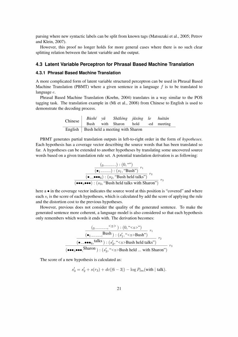
Phrasal Based Machine Translation (Koehn, 2004) translates in a way similar to the POStagging task. The translation example in (Mi et al., 2008) from Chinese to English is used todemonstrate the decoding process.

ChineseBushı yu Shalong juxıng le huıtanBush with Sharon hold -ed meeting

English Bush held a meeting with Sharon

PBMT generates partial translation outputs in left-to-right order in the form of hypotheses.Each hypothesis has a coverage vector describing the source words that has been translated sofar. A hypotheses can be extended to another hypotheses by translating some uncovered sourcewords based on a given translation rule set. A potential translation derivation is as following:

(0 ) : (0, “”)

(•1 ) : (s1, “Bush”)r1

(• •••6) : (s2, “Bush held talks”)r2

(•••3•••) : (s3, “Bush held talks with Sharon”)r3

here a • in the coverage vector indicates the source word at this position is “covered” and whereeach si is the score of each hypotheses, which is calculated by add the score of applying the ruleand the distortion cost to the previous hypotheses.

However, previous does not consider the quality of the generated sentence. To make thegenerated sentence more coherent, a language model is also considered so that each hypothesisonly remembers which words it ends with. The derivation becomes:

(0 ,<s> ) : (0, “<s>”)

(•1 ,Bush ) : (s′1, “<s>Bush”)r1

(• •••6,talks ) : (s′2, “<s>Bush held talks”)r2

(•••3•••,Sharon ) : (s′3, “<s>Bush held ... with Sharon”)r3

The score of a new hypothesis is calculated as:

s′3 = s′2 + s(r3) + dc(|6− 3|)− logPlm(with | talk).

21

0 1 2 3 4 5 6

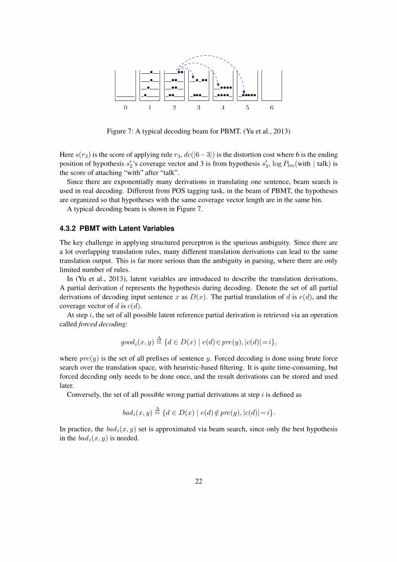
Figure 7: A typical decoding beam for PBMT. (Yu et al., 2013)

Here s(r3) is the score of applying rule r3, dc(|6−3|) is the distortion cost where 6 is the endingposition of hypothesis s′2’s coverage vector and 3 is from hypothesis s′3, logPlm(with | talk) isthe score of attaching “with” after “talk”.

Since there are exponentially many derivations in translating one sentence, beam search isused in real decoding. Different from POS tagging task, in the beam of PBMT, the hypothesesare organized so that hypotheses with the same coverage vector length are in the same bin.

A typical decoding beam is shown in Figure 7.

4.3.2 PBMT with Latent Variables

The key challenge in applying structured perceptron is the spurious ambiguity. Since there area lot overlapping translation rules, many different translation derivations can lead to the sametranslation output. This is far more serious than the ambiguity in parsing, where there are onlylimited number of rules.

In (Yu et al., 2013), latent variables are introduced to describe the translation derivations.A partial derivation d represents the hypothesis during decoding. Denote the set of all partialderivations of decoding input sentence x as D(x). The partial translation of d is e(d), and thecoverage vector of d is c(d).

At step i, the set of all possible latent reference partial derivation is retrieved via an operationcalled forced decoding:

good i(x, y)∆= {d ∈ D(x) | e(d)∈pre(y), |c(d)|= i},

where pre(y) is the set of all prefixes of sentence y. Forced decoding is done using brute forcesearch over the translation space, with heuristic-based filtering. It is quite time-consuming, butforced decoding only needs to be done once, and the result derivations can be stored and usedlater.

Conversely, the set of all possible wrong partial derivations at step i is defined as

bad i(x, y)∆= {d ∈ D(x) | e(d) /∈pre(y), |c(d)|= i}.

In practice, the bad i(x, y) set is approximated via beam search, since only the best hypothesisin the bad i(x, y) is needed.

22

The structured perceptron with early update strategy can be defined as

d+i (x, y)

∆= argmax

d∈goodi(x,y)w ·Φ(x, d)

d−i (x, y)∆= argmax

d∈badi(x,y)w ·Φ(x, d)

w← w + ∆Φ(x, d+i (x, y), d−i (x, y))

where i is chosen as the first step where all reference partial derivation falls out of the beam.Similarly, max-violation latent variable perceptron is defined as

i∗∆= argmin

iw ·∆Φ(x, d+

i (x, y), d−i (x, y))

w← w + ∆Φ(x, d+i∗(x, y), d−i∗(x, y))

where i is chosen as the step where the score difference between the best partial reference deriva-tion and the best partial Viterbi derivation is maximum.

Max-violation latent variable perceptron shows significant improvement over existing opti-mization methods for PBMT. However, as mentioned in Section 4.2, there is not theoreticalproof for the convergence of perceptron with such kind of latent variables.

4.4 Other Applications

The complicated latent variable perceptron is a very general model that can be applied in manydifferent tasks.

4.4.1 Syntax Based Machine Translation

Syntax Based Machine Translation (SBMT) (Wu, 1997; Chiang, 2007) has a longer history thanPBMT. (Zhao et al., 2014) extend latent variable structured perceptron to SBMT.

The difference between latent variable structured perceptron for SBMT and PBMT is similarto the difference between structured perceptron for incremental parsing and bottom-up parsing:in PBMT, the derivation is a sequence, while in SBMT, the derivation is a hypergrah. So that inSBMT, the partial derivation is defined over hypergraph nodes, rather than steps.

In general, latent variable structured perceptron for SBMT is similar to the structured per-ceptorn for bottom-up syntactic parsing with forest in Section 3.6.2 (Zhang et al., 2013). Thedifference is that the partial reference derivations are latent, so forced decoding process is stillrequired.

4.4.2 Semantic Parsing

Semantic parsing is another task where latent variables are widely used.In general, semantic parsing parses an input sentence x into meaning representations like

logic expression (Tang and Mooney, 2001), lambda expression (Zettlemoyer and Collins, 2005),or other variants (Berant et al., 2013).

23

Here is an example of semantic parsing using the meaning representation of lambda expres-sion:

input What is the capital of the largest state by area?output (capital (argmax state size))

Supervised Semantic ParsingIn the supervised semantic parsing, both the input sentence and the output meaning represen-

tations are known. The task is similar to machine translation: the input is a sentence in commonlanguage, the output is a tree structure in the language of the chosen meaning representation.

However, semantic parsing is usually more challenging than machine translation. In machinetranslation, the translation rules are usually collected from large parallel bilingual corpus, andthe only hidden part is how to choose and organize appropriate rules to generate the desiredoutput. In semantic parsing, even the translation rules are hidden and need to be learned duringthe training.

With latent variable structured perceptron, the latent variables represent the hidden referencederivations including the necessary rules being used. The training process is similar to machinetranslation.

The idea of latent variable in semantic parsing training is used in most of current semanticparsing learners (Zettlemoyer and Collins, 2005; Berant et al., 2013; Kwiatkowski et al., 2013),but sometimes not explicitly mentioned.Weakly-Supervised Semantic Parsing

Semantic parsers can also be trained in a weakly-supervised setting where the input sentencesare questions, output meaning representations are missing, and only the answers to the input areknown.

Weakly-supervised semantic parsing has more spurious ambiguity, since different meaningrepresentations including incorrect ones can give the same correct answer. Thus the searchspace for weakly-supervised learning is a lot larger than the supervised setting.

5 Conclusion

In this survey how perceptron can be extended to handle structured prediction problem is exam-ined.

Simple as it is, perceptron is capable of handling most of structured prediction tasks in NLPfield. Unlike its applications in other fields like computer vision where a simple linear model isusually weak in handling hard problems, so that advanced techniques like kernel are developed,perceptron performs well in NLP. This might be explained by that the sparse features speciallydesigned for each task is usually powerful enough to make the system linear separable, or almostlinear separable, so that a simple linear model can solve most of the problems. In addition, moststructured prediction problems in NLP usually involve huge data, while handling huge data isone specialty of perceptron, compared to other learning methods like SVM or CRF that is hardto scale.

24

References

Altmann, G. and Steedman, M. (1988). Interaction with context during human sentence pro-cessing. Cognition, 30(3):191–238.

Berant, J., Chou, A., Frostig, R., and Liang, P. (2013). Semantic parsing on freebase fromquestion-answer pairs. In EMNLP, pages 1533–1544.

Chiang, D. (2007). Hierarchical phrase-based translation. computational linguistics, 33(2):201–228.

Collins, M. (2002). Discriminative training methods for hidden markov models: Theory andexperiments with perceptron algorithms. In Proceedings of EMNLP.

Collins, M. and Roark, B. (2004). Incremental parsing with the perceptron algorithm. In Pro-ceedings of the 42nd Annual Meeting on Association for Computational Linguistics, page111. Association for Computational Linguistics.

Daume, H. C. (2006). Practical structured learning techniques for natural language processing.ProQuest.

Freund, Y. and Schapire, R. E. (1999). Large margin classification using the perceptron algo-rithm. Machine learning, 37(3):277–296.

Huang, L. (2008). Forest reranking: Discriminative parsing with non-local features. In ACL,pages 586–594. Citeseer.

Huang, L., Fayong, S., and Guo, Y. (2012). Structured perceptron with inexact search. InProceedings of the 2012 Conference of the North American Chapter of the Association forComputational Linguistics: Human Language Technologies, pages 142–151. Associationfor Computational Linguistics.

Huang, Z., Eidelman, V., and Harper, M. (2009). Improving a simple bigram hmm part-of-speech tagger by latent annotation and self-training. In Proceedings of Human LanguageTechnologies: The 2009 Annual Conference of the North American Chapter of the Asso-ciation for Computational Linguistics, Companion Volume: Short Papers, pages 213–216.Association for Computational Linguistics.

Joshi, A. K., Levy, L. S., and Takahashi, M. (1975). Tree adjunct grammars. Journal of computerand system sciences, 10(1):136–163.

Klein, D. and Manning, C. D. (2005). Parsing and hypergraphs. In New developments in parsingtechnology, pages 351–372. Springer.

Koehn, P. (2004). Pharaoh: a beam search decoder for phrase-based statistical machine transla-tion models. In Machine translation: From real users to research, pages 115–124. Springer.

Kwiatkowski, T., Choi, E., Artzi, Y., and Zettlemoyer, L. (2013). Scaling semantic parsers withon-the-fly ontology matching.

25

Lafferty, J., McCallum, A., and Pereira, F. C. (2001). Conditional random fields: Probabilisticmodels for segmenting and labeling sequence data.

Liang, P. (2013). Lambda dependency-based compositional semantics. arXiv preprintarXiv:1309.4408.

Marcus, M. P., Marcinkiewicz, M. A., and Santorini, B. (1993). Building a large annotatedcorpus of english: The penn treebank. Computational linguistics, 19(2):313–330.

Matsuzaki, T., Miyao, Y., and Tsujii, J. (2005). Probabilistic cfg with latent annotations. InProceedings of the 43rd Annual Meeting on Association for Computational Linguistics,pages 75–82. Association for Computational Linguistics.

McDonald, R., Pereira, F., Ribarov, K., and Hajic, J. (2005). Non-projective dependency pars-ing using spanning tree algorithms. In Proceedings of the conference on Human LanguageTechnology and Empirical Methods in Natural Language Processing, pages 523–530. As-sociation for Computational Linguistics.

Mi, H., Huang, L., and Liu, Q. (2008). Forest-based translation. In ACL, pages 192–199.Citeseer.

Nivre, J. (2003). An efficient algorithm for projective dependency parsing. In Proceedings ofthe 8th International Workshop on Parsing Technologies (IWPT. Citeseer.

Papineni, K., Roukos, S., Ward, T., and Zhu, W.-J. (2002). Bleu: a method for automaticevaluation of machine translation. In Proceedings of the 40th annual meeting on associationfor computational linguistics, pages 311–318. Association for Computational Linguistics.

Petrov, S. and Klein, D. (2007). Discriminative log-linear grammars with latent variables. InAdvances in Neural Information Processing Systems, pages 1153–1160.

Rosenblatt, F. (1957). The perceptron, a perceiving and recognizing automaton Project Para.Cornell Aeronautical Laboratory.

Sun, X., Matsuzaki, T., Okanohara, D., and Tsujii, J. (2009). Latent variable perceptron algo-rithm for structured classification. In IJCAI, volume 9, pages 1236–1242.

Sutton, C. and McCallum, A. (2010). An introduction to conditional random fields. arXivpreprint arXiv:1011.4088.

Tang, L. R. and Mooney, R. J. (2001). Using multiple clause constructors in inductive logicprogramming for semantic parsing. In Machine Learning: ECML 2001, pages 466–477.Springer.

Taskar, B., Guestrin, C., and Koller, D. (2003). Max-margin markov networks. In Advances inNeural Information Processing Systems, page None.

Tsochantaridis, I., Joachims, T., Hofmann, T., and Altun, Y. (2005). Large margin methods forstructured and interdependent output variables. In Journal of Machine Learning Research,pages 1453–1484.

26

Wu, D. (1997). Stochastic inversion transduction grammars and bilingual parsing of parallelcorpora. Computational linguistics, 23(3):377–403.

Xue, N., Xia, F., Chiou, F.-D., and Palmer, M. (2005). The penn chinese treebank: Phrasestructure annotation of a large corpus. Natural language engineering, 11(02):207–238.

Yu, H., Huang, L., Mi, H., and Zhao, K. (2013). Max-violation perceptron and forced decodingfor scalable mt training. In EMNLP, pages 1112–1123.

Zettlemoyer, L. S. and Collins, M. (2005). Learning to map sentences to logical form: Structuredclassification with probabilistic categorial grammars. UAI.

Zhang, H., Huang, L., Zhao, K., and McDonald, R. (2013). Online learning for inexact hyper-graph search. In Proceedings of EMNLP.

Zhao, K., Huang, L., Mi, H., and Ittycheriah, A. (2014). Hierarchical mt training using max-violation perceptron.

27