study of water quality in urban streams: mätäjoki and
TRANSCRIPT

Shree Ram Bhusal
Study of Water Quality in Urban Streams: Mätäjoki and Haaganpuro
Helsinki Metropolia University of Applied Sciences
Bachelor’s Degree
Environmental Engineering
Thesis
18 June 2017

Abstract
Author(s) Title Number of Pages Date
Shree Ram Bhusal Study of Water Quality in Urban Streams: Mätäjoki and Haagan-puro 61 pages + 9 appendices 18 June 2017
Degree Bachelor’s Degree
Degree Programme Environmental Engineering
Specialisation option Water and Waste Management
Instructor(s)
Kaj Lindedahl, Senior Lecturer (Supervisor)
Johanna Kortesalmi, Laboratory Instructor
Mätäjoki and Haaganpuro have been important urban streams in Helsinki in terms of their
ecological and recreational values. These streams have been well known as a spawning
place for trout. They have been home to many flora and fauna and carry a significance
importance in the surrounding ecosystem.
The main aim of this thesis was to study the current condition of water quality in these
streams in terms of physical and chemical parameters that include temperature, pH, electri-
cal conductivity, dissolved oxygen, turbidity, total iron, total phosphorus and total nitrogen.
First, literature review was done to know about parameters and their effects on water quality.
Parameters such as temperature, pH, electrical conductivity, dissolved oxygen were deter-
mined onsite and other parameters such as nutrients, iron and turbidity were determined in
the Environmental Engineering Laboratory of Metropolia University of Applied Sciences.
Five water samples of each streams were taken from five different locations of streams for
the chemical analysis.
The result shows that the overall water quality of Mätäjoki and Haaganpuro is good. Con-
centration of dissolved oxygen was found to be very low in the first two sampling sites of
Mätäjoki. Average concentration of total phosphorus in Mätäjoki is more than it was in 1995-
1996 and 2004. Haaganpuro has better water quality than Mätäjoki.
Keywords urban streams, Mätäjoki, Haaganpuro, water quality monitor-ing, water quality parameters

ACKNOWLEDGEMENTS
I would like to express my sincere gratitude to Metropolia University of Applied Sciences
for letting me fulfill my dream of becoming an Environmental Engineer. I would like to
take this opportunity to express my immense gratitude to my supervisor, teachers,
friends and all those persons who helped me during my thesis.
In particular, I am grateful to my supervisor, Mr. Kaj Lindedahl who was very generous
with his time and knowledge and helped me with every step of my thesis. Secondly, I
would like to thank my laboratory teacher, Mrs. Johanna Kortesalmi, who continuously
helped me with the laboratory work. I would also like to thank Dr Minna Paananen Porkka
for her help and guidance in thesis writing.
I am fully responsible for any kind of errors and any grammatical and spelling mistakes
in my thesis report. Finally, I want to dedicate this thesis to my mother who believed in
me and always supported and encouraged me in every step of my life.
June 2017,
Shree Ram Bhusal

Table of Contents
List of Figures a
List of Tables b
List of Abbreviations c
List of Symbols d
1 INTRODUCTION 1
1.1 Mätäjoki 1
1.2 Haaganpuro 2
1.3 Objectives 3
1.4 Background 4
2 LITERATURE REVIEW 4
2.1 Water quality and parameters 4
2.1.1 Temperature 5
2.1.2 pH 7
2.1.3 Electrical conductivity 10
2.1.4 Dissolved oxygen 13
2.1.5 Turbidity 18
2.1.6 Metals 21
2.1.7 Nutrients 23
3 MATERIALS AND METHODOLOGY 31
3.1 Sampling sites and conditions 31
3.1.1 Weather 33
3.1.2 Equipment used 33
3.1.3 Sampling procedures 34
3.2 Onsite measurements 34
3.2.1 Procedures 34
3.3 Laboratory measurements 35
3.3.1 Equipment used 35
3.3.2 Chemicals used 36
3.3.3 Procedures 36
3.4 Safety precautions 40
4 RESULTS 41

4.1 Mätäjoki 41
4.2 Haaganpuro 42
5 DISCUSSION 44
5.1 Mätäjoki VS Haaganpuro 44
5.2 Water quality of Mätäjoki (1995-2016) 45
5.3 Water quality of Haaganpuro (1987-2016) 48
6 CONCLUSION 51
References 52
Appendices i
Appendix A: Method settings during iron test using Agilent 4100 MP-AES technology i
Appendix B: Results obtained during iron test using Agilent 4100 MP-AES technology ii
Appendix C: Water quality of Mätäjoki (1982-2005) iii
Appendix D: Water quality of Haaganpuro (1982-2005) iv
Appendix E: Water quality of Mätäjoki and Haaganpuro in 2004 v
Appendix F: Nutrients concentration in Mätäjoki and Haaganpuro in 2004 vi
Appendix G: Sampling sites of Mätäjoki vii
Appendix H: Sampling sites of Haaganpuro viii
Appendix I: Instruments used during onsite measurements ix

a
List of Figures
Figure 1. Mätäjoki stream ............................................................................................. 2
Figure 2. Haaganpuro stream ....................................................................................... 3
Figure 3. Relation between water temperature and metabolic rate of aquatic organisms
..................................................................................................................................... 6
Figure 4. Relation between pH and water temperature ................................................. 9
Figure 5. Relation between water temperature and solubility of salts .......................... 13
Figure 6. Range of tolerance for DO in fish ................................................................. 14
Figure 7. Relation between DO and water temperature .............................................. 17
Figure 8. Relation between turbidity and streamflow ................................................... 19
Figure 9. Nitrogen cycle .............................................................................................. 24
Figure 10. Phosphorus cycle ...................................................................................... 27
Figure 11. P and N discharges into surface waters from point sources in Finland (1980-
2015) .......................................................................................................................... 28
Figure 12. Total P and N discharge from Finnish rivers into Baltic Sea (1979-2015) ... 30
Figure 13. Sampling sites of Mätäjoki ......................................................................... 32
Figure 14. Sampling sites of Haaganpuro ................................................................... 33
Figure 15. Iron test using 4100 MP-AES technology ................................................... 38
Figure 16. Nitrogen and phosphorus test using Hach/Lange Spectrophotometer DR 3900
................................................................................................................................... 39
Figure 17. Electrical conductivity in Mätäjoki (1995-2016) ........................................... 46
Figure 18. DO and turbidity level in Mätäjoki (1995-2016) ........................................... 47
Figure 19. Total N and Total P concentration in Mätäjoki (1995-2016) ........................ 47
Figure 20. Electrical conductivity in Haaganpuro (1987-2016) .................................... 49
Figure 21. DO and turbidity level in Haaganpuro (1987-2016) .................................... 49
Figure 22. Total N and Total P concentration in Haaganpuro (1987-2016) ................. 50

b
List of Tables
Table 1. Value of Kw, pH and pOH in different temperatures ...................................... 10
Table 2. Normal tolerance of different aquatic organisms to temperature and DO ...... 15
Table 3. Sampling sites, their location and sampling time for Mätäjoki ........................ 31
Table 4. Sampling sites, their location and sampling time for Haaganpuro ................. 32
Table 5. Results of onsite measurements of Mätäjoki ................................................. 41
Table 6. Results of laboratory measurements of Mätäjoki ........................................... 42
Table 7. Results of onsite measurements of Haaganpuro ........................................... 43
Table 8. Results of laboratory measurements of Haaganpuro .................................... 44

c
List of Abbreviations
AA Atomic Absorption
AAS Atomic Absorption Spectroscopy
AES Atomic Emission Spectroscopy
Aq. Aqueous
ATP Adenosine Tri-Phosphate
CCD Charge Coupled Device
DNA Deoxyribonucleic Acid
DO Dissolved Oxygen
EU European Union
FTU Formazin Turbidity Units
g gas
ICP-AES Induced Couple Plasma Atomic Emission Spectroscopy
K Kelvin
I liquid
MP-AES Microwave Plasma Atomic Emission Spectroscopy
nm nanometer
NTU Nephelometric Turbidity Units
pH Potential Hydrogen
pm Picometer
ppb Parts per billion
ppm Parts per million
S Siemens
TDS Total Dissolved Solids
UV Ultraviolet
vs Versus
WHO World Health Organization

d
List of Symbols
H2O Water
H2SO4 Sulfuric acid
CO2 Carbon dioxide
C6H12O6 Glucose
Fe Iron
Kw Ionization constant of water
l/s Liter per second
SO2 Sulfur dioxide
S/cm Siemens per centimeter
S/m Siemens per meter
dS/cm deci Siemens per centimeter
µS/cm micro Siemens per centimeter
mg/l milligram per liter
µg/l microgram per liter
NH3 Ammonia
NH4+ Ammonium ion
NO Nitrogen Oxide
NO2- Nitrite ion
NO3- Nitrate ion
Fe(OH)2+ Ferrous Hydroxide
N Nitrogen
P Phosphorus
PO4 3- Ortho-phosphate
HPO4 2- Hydrogen Phosphate
H2PO4 – Dihydrogen Phosphate

1
1 INTRODUCTION
Urban streams are a natural component of hydrological cycle that play a significant role
in urban environment and community. Good ecological status of urban streams in-
creases biodiversity and act as a recreational area for the local community. Testing of
water quality of urban streams has been one of the important part of monitoring the en-
vironment. Poor water quality not only affects the aquatic life but also affects the ecosys-
tem of surrounding. Monitoring of water quality of urban streams is necessary so that the
researchers can predict and learn from the environment naturally and can determine the
human impact on an ecosystem. [1]
There are more than 25 urban streams in Helsinki. Mätäjoki and Haaganpuro have been
important streams in Helsinki in terms of their ecological and recreational values. They
flow through forests, parks and residential areas. These streams are well known for sea
trout and their ability to provide spawning ground for this fish species.
1.1 Mätäjoki
Mätäjoki is considered as the second largest water flow in Helsinki after the Vantaa river.
It is known to be the former riverbed of Vantaa river. It flows from Louhela and
Kaivoksela, Vantaa from where it flows to the south part of Helsinki via Malminkartano
and Kannelmäki park areas, curves to the west Pitäjänmäki and finally reaches Laajalahti
in the Gulf of Finland through the Iso-Huopalahti area in Helsinki. [2]
Mätäjoki has a catchment area of 24 km2 where about 72000 people live in that area. It
has a large catchment area because Mätäjoki is sensitive to rain that makes it flooded to
overflowing. The length of main channel is about 9 km with the average flow of 170 l/s.
The water quality of Mätäjoki has been reasonably good. Mätäjoki is rich in scrubby veg-
etation due to which it has been home to abundant bird lives. For example, nightingales
are mostly found here, and water birds such as tufted ducks, golden eyed ducks and
aspen witch birds are abundant. Mätäjoki has also been home to water voles. [3]
In 1995-1996, Mätäjoki was found to be polytrophic in terms of nutrient level. Nitrogen
and phosphorous transportation amount was about 330.8 kg/ km2 and 13.4 kg/km2 re-
spectively. The hygienic quality of Mätäjoki was passable during that period. The quality
of water was much better since mid-1970s, and it was passable in terms of its general
grading. [4] Figure 1 shows a photo of Mätäjoki stream near Kannelmäki.

2
Figure 1. Mätäjoki stream
1.2 Haaganpuro
Haaganpuro is the new name of Mätäpuro given to the stream in 1969. It was changed
to Haaganpuro in 2011. The catchment area of Haaganpuro is approximately 10.7 km2.
The main channel of Haaganpuro originates in Maununneva from where it flows to the
south-western part to Maunulan Uurnalehto through Pakila and Pirkkola. Again, from
Maunulan Uurnalehto it flows to southern part through Central Park. In Kivihaantie, the
stream is pipelined below Hämeenlinnanväylä which again flows through Kauppalan-
puisto and finally ends in Pikku Huopalahti. The length of main stream is estimated to be
11.6 km of which below 25% is pipelined. The average flow of Haaganpuro is about 101
l/s. [5] Figure 2 shows a photo of the Haaganpuro stream near Kauppalanpuisto.

3
Figure 2. Haaganpuro stream
Haaganpuro has been known for endangered brown trout, but due to the urbanization,
trout stocks collapsed in the mid-1900s. Trout has been the victim of, for example, poor
water quality of Haaganpuro caused by the sewage leaking into the water, illegal fishing,
construction projects and noise from vehicles. Trout has been seen again in Haaganpuro
successfully in the 2000s as the water quality improved during the last two decades. It
has been used as an urban brook for spawning of sea trout. The trout population has
been reviewed in recent years through fish planting and restorations, and it is seen that
trout has been breeding successfully. Fishing in Haaganpuro is prohibited especially dur-
ing spawning time which is in late autumn. [6] The ecological and recreational value of
Haaganpuro was officially recognized in 2006 by its enclosure into the ambitious Helsinki
small streams program. [7]
1.3 Objectives
Urban streams and their water quality have been important subjects to research in Hel-
sinki in recent years. In the city of Helsinki, the state of the river is observed by the city's
environmental center on a regular basis sampling twice a year.

4
However, until now there has been lack of continuous and regular key research on water
quality of specific streams separately. The main objectives of this thesis were the
following:
• To study the overall condition of water quality of Mätäjoki and Haaganpuro.
• To compare the water quality of these two streams with each other.
• To compare the water quality of these two streams with past data.
• To study the concentration of nutrients in the streams.
• To understand the effects of different parameters in the water quality.
1.4 Background
Mätäjoki and Haaganpuro have been victim of pollution in the past due to various rea-
sons which has affected the aquatic ecosystem as well as surrounding environment. In
May 2013, around 500-1000 liters of solvent, Shellsol A 100 was leaked into Mätäjoki
through storm drain from paint company named Teknos Oy located in Pitäjänmäki due
to the negligence of the employees. Tens of thousands of fishes were found dead be-
cause of the solvent which is toxic to aquatic organisms. [8] This kind of environmental
accidents and other human impacts have regularly degraded the quality of water in the
urban streams. Haaganpuro and Mätäjoki have been home for endangered brown trout.
The trout population has been revived through fish plantations and restorations in recent
years in Haaganpuro and Mätäjoki, with the help of different organizations. Trout popu-
lation carries a constant threat of water quality problem. Although, the quality of water in
Haaganpuro and Mätäjoki is improving, it is still very important to monitor the water qual-
ity, to be sure there is not a problem associated with the trout population and overall
urban ecosystem.
2 LITERATURE REVIEW
2.1 Water quality and parameters
The term water quality is a broad topic so it has different meaning to different people.
Most used definition of water quality is ‘’the chemical, physical and biological character-
istics of water, usually in respect to its suitability for its designated use.’’ Water is used
for various purposes such as drinking, watering animals and plants on farms and raising

5
fish, and these designated uses have their own definition for chemical, physical and bi-
ological standards necessary to support that use. [9]
Water quality of urban streams is affected by both natural and human influences. Most
common natural influences are geological, hydrological and climatic because these in-
fluences affect both the quantity and the quality of water resources. One example of
natural influence is fresh water resources near coastal areas has a problem of high sa-
linity. Human influences such as pollution of water resources by human feces or dis-
charge of industrial water have been the problem especially in the developing countries.
Other reasons for the depletion of water quality of fresh water has been the agricultural
runoff and wastewater discharge that has affected the quality of water by the rising con-
centration of nutrients in the water sources resulting in problems such as eutrophication.
[10]
There are physical, chemical and biological parameters that help to determine the quality
of water resources. Physical parameters, for example, temperature, turbidity, color, taste
and odor explain the physical characteristics of water. These parameters are determined
using senses of touch, sight, smell and taste. Chemical parameters such as pH, electric
conductivity, dissolved oxygen, heavy metals and nutrients explain the chemical charac-
teristics of water and biological parameters help to identify the presence of microorgan-
isms and water borne pathogens in the water. Examples of biological parameters of wa-
ter quality are E. coli and total coliform. This thesis focuses on specific physio-chemical
parameters such as temperature, pH, electrical conductivity, DO, heavy metals (total
iron) and nutrients (total nitrogen and total phosphorus) to determine the water quality of
Mätäjoki and Haaganpuro.
2.1.1 Temperature
Water temperature is an important physical property expressing how hot or the cold the
water resources are. It is affected by different factors such as temperature of air, ground-
water inflow, exposure to the sunlight, turbidity and thermal pollution. Temperature plays
an important role in the lives of aquatic animals and plants; thus, it is necessary to con-
sider the maximum and the optimum temperature. Maximum temperature of water is the
highest water temperature in which the aquatic lives can survive for a few hours, whereas
optimum temperature is a suitable temperature for the aquatic lives to survive. Water
temperature is also responsible for affecting the metabolic rates and biological activity of

6
the aquatic lives. It even affects the habitat of aquatic organisms; for example, aquatic
plants are seen mostly in the warmer temperature, whereas fishes such as trout prefer
colder temperature to survive in the water. Water temperature is directly proportional to
the metabolic rate of the organisms as many cellular enzymes are more active in the
warmer temperature. In Figure 3, it is seen that for most of the fishes, rise in 10 OC water
temperature will approximately double the rate of physiological function. Temperature
above 35 OC can result in breakdown of enzymes reducing metabolic function. Plants
are also affected by the water temperature. For example, at temperatures below 21 OC,
tropical plants restrict their growth and dormancy.
Figure 3. Relation between water temperature and metabolic rate of aquatic organisms [11]
Water temperature not only affects the aquatic organisms but also influences other pa-
rameters of water quality such as pH, compound toxicity, DO and other dissolved gas
concentrations, conductivity and salinity, oxidation reduction potential, and water density.
High water temperature can increase the solubility and toxicity of certain compounds, for
example, ammonia and heavy metals such as zinc, cadmium, and lead. High water tem-
perature not only increases the solubility of the compound but also affects the tolerance
limit of the aquatic organisms. Water temperature is directly proportional to the density
of water. The density of pure water decreases approximately by 9% when it freezes
which is the reason why ice expands and float on the water. [11]

7
2.1.2 pH
pH is one of the most common test performed to determine the quality of water. It stands
for ‘power of hydrogen’. It is a measure of how acidic or basic the water is. pH is meas-
ured in the range of 0-14, where 7 is considered as a neutral. If the pH of water is less
than 7, it is considered as acidic, and if it is greater than 7, it is considered as basic. In
other words, pH can be defined as the measure of free hydrogen and hydroxyl ions in
the water. If the water has more hydrogen ions, it is acidic, and if it has more hydroxyl
ions, it is basic. pH is reported in ‘logarithms unit’ where each number represents 10-fold
change in the acidity and basicity of water. As an example, water having pH of 5 is 10
times acidic than the water having pH of 6 and the water having pH of 9 is 10 times more
basic than the water having pH of 8. Molar concentration of hydrogen ions (H+)3 deter-
mines the numerical value of pH which is calculated by taking the negative logarithm of
hydrogen ion concentration (-log(H+)3). For example, if the solution has a concentration
of (H+) = 10-3, the pH of solution is given by
pH= (-log (10-3)), which is equal to 3 and shows that the solution is acidic.
In the case of neutral pH, the concentration of both hydrogen and hydroxyl ion is 10-7;
thus, these ions are always paired, which means concentration of one ion increases
when concentration of other decreases. The sum of ions will always be 10-14 regardless
of the pH. [12]
There is greater importance of pH in determining the quality of water because it deter-
mines the solubility and biological availability of chemical elements, for example, nutri-
ents such as phosphorus, nitrogen and carbon and heavy metals such as lead, copper
and cadmium. For instance, it not only affects the quantity and form of chemical constit-
uent such as phosphorus abundant in the water but also determines if the aquatic life
can use it or not. In case of heavy metals, toxicity is determined by the degree of their
solubility in the water. Metals are usually more toxic in the water with a lower pH as they
are more soluble. [13]
Aquatic organisms live in water with a specific pH. Most aquatic organisms cannot sur-
vive at too low or too high pH. These organisms prefer the optimum condition where the
pH of water lies in the range of 6.5-9. If the aquatic organism is sensitive, it is more
affected by the change in the pH of water. An extreme pH of water can increase the
solubility of different chemical elements making the water toxic, which increases the risk

8
of absorption by the aquatic organisms. A slight change in pH level can cause eutrophi-
cation in the water resources. At a certain level of pH, the solubility of nutrients such as
phosphorus is high and these nutrients are absorbed by the aquatic plants, for example,
algae consuming a high amount of dissolved oxygen for their growth. This finally results
in an overgrowth of those plants in the water resources demanding more dissolved oxy-
gen. Lack of dissolved oxygen in the water resources causes death of aquatic organisms.
Not only aquatic organisms but also human beings are affected by certain pH levels.
Water with a pH greater than 11 and less than 4 can cause eye and skin irritations.
Similarly, water with a pH less than 2.5 will cause irreversible damage to skin and organ
linings. [12]
pH is affected by many factors and those factors are natural and man-made. Most of the
natural changes take place due to the interaction of water sources with the surrounding
rocks and other materials. Precipitation such as acid rain can also change the pH of
water resources making it more acidic and the concentration of carbon-dioxide can alter
the level of pH. Carbon dioxide is considered as one of the major factors affecting the
pH of water. Carbon dioxide has been increasing in the atmosphere due to the reason
of global warming and the dissolved CO2 shows inverse relationship with the pH. That
means higher the concentration of dissolved carbon dioxide in the water lower the pH is.
In other words, we can say water with high concentration of dissolved CO2 is acidic in
nature. Carbon dioxide is released to the water resources, for example, from the atmos-
phere, through surface runoff and by respiring aquatic animals and microbes. Another
factor affecting the pH of water is acid rain resulting from pollution caused by humans. It
is caused when sulfur dioxide (SO2) reacts with nitrogen oxide (NO) in atmosphere com-
bining with water vapor. Acid rain is one reason for water resources being acidic. Dis-
solved minerals from groundwater, where there is limestone bedrock can increase the
alkalinity of water by raising the pH level, and wastewater discharge from individuals,
industries, and municipalities containing different chemicals, for instance, cleaning
agents and detergents increase the alkalinity of the water resources. [14]
In addition, temperature affects the pH of water. Temperature and pH are inversely re-
lated to each other. With the increase in the temperature, the pH of water decreases and
with the decrease of the temperature, the pH of water increases. At pH 7, both hydrogen
and hydroxyl ions have concentrations of 1*10-7 M making the solution neutral, which is
only true at the temperature of 25 OC. Increase or decrease in the temperature of water
shifts the concentration of ions shifting the pH value which is explained by Le-Chatelier’s
Principle.
9
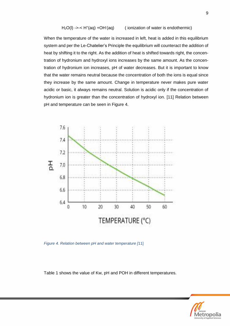
H2O(l) ->-< H+(aq) +OH-(aq) ( ionization of water is endothermic)
When the temperature of the water is increased in left, heat is added in this equilibrium
system and per the Le-Chatelier’s Principle the equilibrium will counteract the addition of
heat by shifting it to the right. As the addition of heat is shifted towards right, the concen-
tration of hydronium and hydroxyl ions increases by the same amount. As the concen-
tration of hydronium ion increases, pH of water decreases. But it is important to know
that the water remains neutral because the concentration of both the ions is equal since
they increase by the same amount. Change in temperature never makes pure water
acidic or basic, it always remains neutral. Solution is acidic only if the concentration of
hydronium ion is greater than the concentration of hydroxyl ion. [11] Relation between
pH and temperature can be seen in Figure 4.
Figure 4. Relation between pH and water temperature [11]
Table 1 shows the value of Kw, pH and POH in different temperatures.

10
Table 1. Value of Kw, pH and pOH in different temperatures [15]
T (OC) Kw (mol2 dm-6) pH pOH
0 0.114 x 10⁻¹⁴ 7.47 7.47
10 0.293 x 10⁻¹⁴ 7.27 7.27
20 0.681 x 10⁻¹⁴ 7.08 7.08
25 1.008 x 10⁻¹⁴ 7.00 7.00
30 1.471 x 10⁻¹⁴ 6.92 6.92
40 2.916 x 10⁻¹⁴ 6.77 6.77
50 5.476 x 10⁻¹⁴ 6.63 6.63
100 51.3 x 10⁻¹⁴ 6.14 6.14
In Figure 4 and Table 1, we can see that the value of pH and pOH is increasing with the
increase of the temperature. We can also see that the value of pH and pOH are same
for the same temperature which is because the concentration of hydrogen and hydroxyl
ions increase by the same amount with the increase of the temperature. We can see that
the value of pH is below 7 from temperature 30 OC to 100 OC; however, we cannot con-
clude that the water is acidic at those temperatures. For the water to be acidic, pH should
be below 7 only when the temperature is at 25 OC. [15]
2.1.3 Electrical conductivity
Conductivity of water is a measure of capability of water to pass an electrical flow. It is
measured in the unit, Siemens per meter (S/m) in SI unit. For the measurement of fresh-
water, micro Siemens per centimeter is the standard unit. Conductivity is denoted by the
symbol k or s.
Conductivity is directly related with the concentration of ions in the water solution, and
these ions come from dissolved salts and inorganic substances in the water, for example,
alkalis, sulfides, chlorides and carbonated compounds. These compounds are also
known as electrolytes that dissolve in the water as ions. Electrical conductivity of water
is high when there are more free ions present in the water and conductivity is low when

11
the number of free ions present in the water is low. Ions can conduct electricity because
they have positive and negative charges. Therefore, when electrolytes dissolve in the
water, they split into positive and negative charges. Positive charge is known as cation
and negative charge is known as anion. Concentrations of each positive and negative
charge remain equal when the electrolytes split in the water, which means water remains
electrically neutral although water’s conductivity increases with added ions. [16]
Pure water is a bad conductor of electricity because the concentration of free ions in the
pure water is very low. Ordinary distilled water in equilibrium with carbon dioxide in the
atmosphere has a conductivity of 20 dS/m. Typical Conductivity for several types of water
are listed below:
• Ultra-pure water: 5.5 x 10⁻⁶ S/m
• Drinking water: 0.005-0.05 S/m
• Seawater: 5 S/m
Seawater has a high conductivity due to the greater number of free ions present in the
water because of salt present in the sea water. [17]
The main source of conductivity in fresh water is the geology of surrounding environment.
Clay soil is one of the source that increase the conductivity of water. The minerals pre-
sent in the clay are ionized as they dissolve in the water. Similarly, the groundwater that
flows to the freshwater sources also contribute to the conductivity depending on the ge-
ology of the groundwater. If the groundwater is rich in minerals that can ionize, it will
increase the conductivity of fresh water source where it flows.
Conductivity is an important parameter to determine the water quality. It shows an early
indication if there is any change in the water system. Most of the water bodies uphold
constant conductivity so it can be used as a reference line of evaluation for the future
measurements. If there is any notable change in conductivity of water resources, we can
predict that the change is caused by several reasons such as pollution, flooding and
evaporation, and this will help to minimize those environmental problems to maintain the
good water quality. Conductivity and salinity are strongly correlated to each other so
salinity and TDS which affect water quality can be estimated easily with the help of con-
ductivity. Salinity is important because it affects the solubility of dissolved oxygen. The
higher the salinity of water, the lower the concentration of dissolved oxygen in water. At
the same temperature oxygen is about 20% less soluble in seawater than in fresh water.
[16]

12
Conductivity is an indirect measurement of water salinity. Aquatic organisms such as
fishes that survive in fresh water cannot tolerate a significant increase in the salinity of
water because they cannot keep water in their bodies. Thus, high conductivity of water
means the more negative effect to aquatic organisms. [18]
Factors affecting conductivity
There are numerous factors responsible for the change in conductivity of water. The
main reasons for the fluctuation of conductivity are temperature and salinity/TDS. Con-
ductivity of water fluctuates daily because of temperature. Water flows from one source
to another and water level also affect the conductivity of water because of their impact
on salinity of water. Change in water level due to evaporation of water will increase the
salinity and conductivity of water. Similarly, the rain can increase the water level that
decrease the conductivity of water. [16]
Water temperature and conductivity are related with each other. Increase in the water
temperature will cause a decrease in the viscosity of water and an increase in the mobility
of ions in a water. Also, the increase in the temperature of water can cause an increase
in the number of ions in a water solution because of separation of molecules. As con-
ductivity is directly related to the number of ions and their mobility in the solution, increase
in the water temperature will increase the conductivity of the water. [19]
There is approximately 2-3% increase in the conductivity with 1 OC increase in the tem-
perature, where in case of pure water it increases by 5% with 1 OC increase in the tem-
perature. This is the reason why many professionals use specific conductance, which is
a standardized comparison of conductivity that is temperature corrected to 25 OC. Sol-
ubility of many salts is directly proportional to the temperature of water. Higher the tem-
perature of the water, more salts are soluble in the water. Water with a higher tempera-
ture can dissolve several minerals and salts more easily than the water with a low tem-
perature. Increased minerals and ions content can be seen in natural hot springs which
has healing abilities. Among different salts there are some salts that are less soluble in
warmer temperature that inversely affect the conductivity which can be seen below in
the Figure 5. [20]

13
Figure 5. Relation between water temperature and solubility of salts [21]
2.1.4 Dissolved oxygen
It is the amount of oxygen molecule that is dissolved in the water. It is measured in milli-
grams per liter. The oxygen gets dissolved into the water by different process, for exam-
ple, diffusion from the surrounding air, aeration into the water and as a waste product of
photosynthesis.
Photosynthesis in the present of light and chlorophyll gives:
6CO2 + 6H2O C6H12O6 + 6O2
Aquatic animals such as fishes cannot split oxygen from the water molecules (H2O) or
from other oxygen-containing compounds. Oxygen can be split from those compounds
with the help of green plants and some bacteria through the process of photosynthesis
and other similar process. Oxygen is one of the most essential element for the aquatic
organisms to survive. Without the presence of enough oxygen, aquatic life is not possi-
ble. [22]

14
Dissolved oxygen is one of the most important parameter in determining the quality of
water as it has a huge influence on the organisms living in the water bodies. Amount of
dissolved oxygen needed is different for different species.
Figure 6. Range of tolerance for DO in fish [23]
Trout needs about five to six times more DO when the temperature is at 24 OC in com-
parison when the water temperature is 4 OC. As the metabolic rate increases with the
increase of the water temperature, more amount of DO is needed for the aquatic organ-
isms such as trout to support their increased metabolic rates. Figure 6 shows that the
minimum amount of DO needed for fishes to survive is 4 to 5 mg/l. Fishes cannot survive
in the water having DO below 3 mg/l. DO above 7 mg/l supports growth and activity of
fishes and above 9 mg/l it supports abundant fish populations. Depletion of DO in the
water bodies can cause shifting of the organisms living in the water. In case of a low
level of DO, pollution tolerant organisms, for example, flying larvae and worms will re-
place the organisms such as mayfly nymphs, stonefly nymphs and beetle larvae that
cannot survive in low level of DO. Organisms, for instance, nuisance algae and other

15
anaerobic organisms that does not need oxygen become abundant in the water bodies
where there is very low amount of DO present. Certain type of pollutants present in the
water can restrict the oxygen uptake and metabolism. So, if such pollutants are present
in the water, some aquatic organisms may need higher level of DO. [23]
One of the way to assess the quality of water bodies with fair accuracy is by witnessing
the population of aquatic organisms. Table 2 indicates the normal tolerance of different
organisms to temperature and DO levels.
Table 2. Normal tolerance of different aquatic organisms to temperature and DO [24]
Aquatic Organism Temperature Range (OC) Minimum DO level (mg/l)
Trout 5-20 6.5
Smallmouth bass 5-28 6.5
Caddisfly larvae 10-25 4.0
Mayfly larvae 10-25 4.0
Stonefly larvae 10-25 4.0
Catfish 20-25 2.5
Carp 10-25 2.0
Mosquito 10-25 1.0
Water boatmen 10-25 2.0
Concentration of dissolved oxygen also affects some chemicals present in the water. As
an example, some metals, for example, cadmium solidify and sink out of water in the
presence of oxygen and without oxygen such metal dissolves into the water in a form
which is highly poisonous to aquatic organisms. [25]
Factors affecting DO in water
There are both natural and human factors responsible for the change of DO in the water
resources. Natural factors include the following:
• Aquatic life: Aquatic organisms use oxygen for their survival. Organisms such as
bacteria need oxygen to decompose the materials. So, the water containing

16
large amount of dead and decomposing materials have low level of DO as most
of the DO is used by the bacteria.
• Flow and velocity of water: Fast moving streams have high level of DO as run-
ning water is aerated with bubbles as it agitates over rocks and falls down hun-
dreds of tiny waterfalls. In slow and stationary water, oxygen enters only at the
top layer of the water. The deeper part of the water is very low in DO because
bacteria that live at the bottom of the water use oxygen for the decomposition of
organic matters.
• Climate/Season: More oxygen can be dissolved in the cold water. So, the level
of DO in a certain place is higher in winter than in the summer.
• Altitude: Oxygen is dissolved more easily in the water which are at low altitude
than in high altitudes because low altitudes have higher atmospheric pressure.
• Vegetation: Riparian vegetation helps in increase of DO level in the water bodies
by releasing oxygen during the process of photosynthesis. Also, the vegetation
shading helps to decrease the temperature of water bodies. As the DO is in-
versely related with the water temperature, decrease in the temperature of water
bodies will increase the level of DO in the water.
• Groundwater inflow: Although the groundwater has low level of DO than the
stream, it helps to increase the DO in stream by cooling the water of stream as
it is colder than the stream. Low temperature of water means high level of DO.
Human factors responsible for the change in DO level in the water resources are as
follows:
• Destruction of Riparian vegetation: Destruction of such vegetation by human de-
pletes the level of DO in the water. Destruction of vegetation decrease the
amount of shade that increase the temperature of water finally decreasing the
level of DO in the water. And when there is no vegetation, it means there is no
photosynthesis and no photosynthesis means, there is not any release of oxy-
gen.

17
• Nutrient pollution: Nutrients such as phosphorous and nitrogen get into the water
bodies because of human activities such as agriculture and industries. Such nu-
trients get into the water bodies due to land runoff and industrial water discharge.
When concentration of nutrients is high in the water, it supports the growth of
algae blooms. When the algae die, bacteria use lot of DO to decompose algae
resulting in low level of DO in the water.
• Clearing land: Clearance of land for various purposes such as construction and
logging may transport excess amount of organic matters into the water bodies.
Organic matters are decomposed by the microorganisms such as bacteria. So,
high amount of organic matter in the water result in high consumption of DO by
the microorganisms for the decomposition process.
[26] [27]
In addition, one of the key factor affecting dissolved oxygen in the water bodies is tem-
perature. Dissolved oxygen is inversely proportional to the temperature. The solubility of
oxygen and other gases decreases when the temperature of water increases. So, the
colder water can hold more DO than the warmer water. Figure 7 shows the relation be-
tween the water temperature and the oxygen content of the river. [28]
Figure 7. Relation between DO and water temperature [28]

18
2.1.5 Turbidity
Turbidity is one of the important physical parameter for the determination of water quality.
It is a cloudiness of water caused by the suspended particles that are usually invisible to
naked eye. Turbidity is an optical feature of water and is an expression of the amount of
light that is dispersed by particles in the water when a light is passed through the water
sample. It is directly related to the intensity of scattered light. Higher intensity of scattered
light means higher turbidity. So, it shows how well the light can pass through the water.
Water contains different solid particles with a different size. Large particles settle at the
bottom due to their high density, whereas small particles get suspended on the surface
and try to settle very slowly. These types of different particles cause water to look unclear
or turbid. [29]
Normally turbidity is measured by an instrument called a Nephelometer. This instrument
measures turbidity in standard Nephelometric Turbidity units (NTU) by determining the
scattering of light. The level of turbidity normally varies from less than 1 NTU in very clear
streams to much greater than 200 NTU in cloudy rivers after floods. [30] The WHO has
established the level of turbidity in the drinking water per which the turbidity of drinking
water should not be greater than 5 NTU and it should ideally be below 1 NTU. [31]
Causes of Turbidity
There are several factors responsible for increase of turbidity in the water. Major factors
are as follows:
• Soil erosion: Heavy rainfall and increase in streamflow can result in the soil ero-
sion. Soil erosion is the shifting away of top layer of soil due to the natural factors.
This shifting away of soil containing particles, for example, clay and slit reaches
to the water resources that increases the suspended particles in the water finally
causing turbidity.
• Urban runoff: Urban runoff of several types contain the suspended solids that
affect the turbidity of the water resources. Urban runoff from roads, rooftops,
agricultural runoff, runoff from industries and water treatment plants cause in-
crease in the turbidity of water resources.
• Industrial waste: Industrial discharge of water containing various pollutants and
particulates larger than 2 microns contribute in concentration of total suspended
solids. Colored wastewater discharge and dyes are example of pollutants that

19
affect turbidity of water. Although the nutrients such as nitrate and phosphorus
are soluble in the water, they are considered as indirect contributor because they
cause algal blooms which affect the turbidity of water.
• Abundant bottom dwellers: Different bottom-dwelling aquatic organisms such as
catfish can increase the turbidity of water resources as they stir up the sediments
present at the bottom of the water resources.
• Algae growth: Excessive algae growth resulting in the algal blooms because of
high concentration of nutrients is one of the contributor to the turbidity. Algal
blooms floating on the water can block the sunlight and can release the toxins
and decrease the level of DO in the water.
Organic matters such as Plankton or decaying of different plant and animal matter that
is suspended in the water can also increase the turbidity of the water. Similarly, the oil
and gas spills on the roads flowing to the water resources along with the rain can also
increase the turbidity of water resources. [32]
One of the key factors that influence the level of turbidity in the water resources is water
flow. Turbidity is directly related with the water flow. Higher flow rates of the water keep
particles suspended in water instead of letting them settle to the bottom. This is the rea-
son why in rivers and streams where the flow is high, turbidity is seen constant. As heavy
rainfall increases the volume and flow of the water, turbidity of water increases as settled
sediments are again re-suspended in the water. Figure 8 shows the relation between the
water flow and turbidity in the stream. [33]
Figure 8. Relation between turbidity and streamflow [33]

20
Impacts of Turbidity
There are physical, chemical and biological effects of turbidity in the water resources.
They are as follows:
• Fine sediments can cause clogging of channel bed, marginal changes to the
stream channel morphology reducing habitat for small fishes and invertebrates.
Also, reduces the permeability of the bed material.
• Increase in the turbidity, increase the temperature of water. Turbidity is the result
of suspended particles in the water. These suspended particles absorb heat from
sunlight more efficiently than the water. Absorbed heat by the particles is trans-
ferred to the water molecules causing increase in the temperature of water re-
sources.
• Increase in turbidity prevents the sufficient light entering the water that affects
the photosynthesis process. Without photosynthesis process, aquatic plants die.
Many aquatic plants are source of food for different aquatic organisms. Death of
these plants causes lack of food to the organisms and affect the food chain.
• As a chemical impact, high turbidity level can decrease the concentration of DO
in the water. This is because increase in the turbidity increase the water temper-
ature and increase in the water temperature decrease the concentration of DO.
Lack of photosynthesis due to turbidity also decline the concentration of DO in
the water resources.
Beside these impacts, high turbidity also causes physical damage to the surface of
leaves by scratch and smothering. It affects the aquatic organisms, for example, salm-
onids and other fish species by interfering with their behavior and growth. It affects by
preventing successful development of fish eggs and larvae. Turbidity also can cause
damage to fish gills by scratching and clogging. Particles of 2-3 p.m. are mostly respon-
sible for the gill abrasion in the salmonids population. High turbidity may also increase
vulnerability of fishes to disease. When mucus separated by fish is in response to high
concentration of suspended solids, there is high chance to attract bacteria and fungus.
[34]

21
2.1.6 Metals
Different type of metals such as iron (Fe), manganese (Mn), zinc(Zn), lead (Pb) and
copper (Cu) are essential in different biochemical process to sustain life in certain con-
centrations. These metals however in high concentrations are toxic to aquatic organisms
and even can be toxic to human beings if they are ingested directly in the water or when
human beings consume aquatic organisms such as fishes living in water of high metal
concentration. The toxicity and bioavailability of metals depend on their oxidation state
and the form they occur. Water soluble metals are more bioavailable and toxic than the
metals which are found in complex form with other molecules or which are adsorbed to
sediment particles. Chemical characteristics of water such as pH, hardness, DO levels
affect metal’s characteristics, for instance, solubility, oxidation state and toxicity. Metals
occur naturally in the water sources from weathering of rocks and soils. Soil erosion and
sedimentation carry these metals into water resources. Another source of metals in water
bodies is waste water effluent, for example, water discharge from different industries.
[35]
Total iron was one of the parameters analyzed during this thesis project. It is the fourth
most abundant element by weight found in earth’s crust. It is present in different quanti-
ties depending on the geological area and other chemical components of water bodies.
Normally it is present in the form of soluble ferrous (Fe++) in groundwater which can be
easily oxidized to insoluble ferric (Fe+++) state when it is exposed to air. Ferrous and ferric
ions are the primary states of concern in the aquatic environments. Iron can be present
in other forms in organic or inorganic wastewater streams. Iron in ferrous state can per-
sist in the water with no DO and generally originates from groundwater wells. Black or
brown marsh of water may contain iron of several mg/l in the presence or absence of DO
which has very tiny effect on the aquatic life. The current limit of iron concentration for
aquatic life is less than 1.0 mg/l based on toxic effects. [36]
The main source of iron in the water bodies is weathering of iron minerals such as mag-
netite, hematite, goethite and siderite which is a natural process. Weathering of these
minerals releases iron in the water bodies. Other ways how iron can get into the water
bodies are industrial discharge, refining of iron ores and soil erosion. Water pollution
related with construction and iron mining can increase the construction of iron in the
water. Iron gets into the groundwater when the soil and rocks containing iron get in con-
tact with the rain water. This water dissolve iron and finally deposit it into the aquifer.
When this groundwater mix with river water, it can increase the iron concentration of river
water. [37]

22
The concentration of iron in the river water is approximately 0.5-1 ppm of iron and the
groundwater contains 100 ppm of iron. Seawater has approximately 1-3 ppb of iron and
the concentration varies for example the concentration of iron in Atlantic and Pacific
Ocean is different. Iron concentration in drinking water may not be more than 200 ppb of
iron. Iron in the water resources is accumulated by the aquatic organisms. Most of the
algae has 20-200 ppm of iron. Brown algae may accumulate iron up to 4000 ppm. Dis-
solved iron can be found as Fe(OH)2+ (aq.) in acidic, neutral and oxygen rich conditions.
Iron does not change in pure water or dry air but when it gets contact with water or moist
air containing oxygen it gets corrode changing its silver color to reddish-brown because
of the formation of hydrated oxides. [38]
A certain concentration of iron is beneficial to aquatic life. Iron promotes enzyme growth
and gives red color to blood. In fresh water, it is an important nutrient for algae and other
organisms that supports their growth. Due to the reason that iron is abundant in the
earth’s crust, it is found in every freshwater environment and is present in higher con-
centration in the water and sediments than other trace metals. Effects of high
concentration of iron are as follows:
• High concentration of iron is toxic to aquatic organisms. When the iron in the
water is at higher level, aquatic organisms cannot process all the iron. The iron
can build up the internal organs of organism finally killing them. Iron toxicity plays
role in damaging DNA and membrane damage of the organisms. Vertebrate
studies have shown that high cellular concentration of iron may cause cell de-
generation. Increase in iron load can significantly change both structure and
function of aquatic ecosystem.
Similarly, high concentration of iron in fish and aquatic plants can harm human
beings when they consume those aquatic organisms affected by high concentra-
tion of iron. [39]
• High concentration of iron increases the growth rate of algae which can result in
algal bloom. Algal bloom can reduce the freshness of the water and it can block
the sunlight passing to the water that can hamper the photosynthesis process
resulting in decline of DO in the water. Increased concentration of iron some-
times increases the acidity of water. Iron contamination can affect the feeding
habit and reproduction of aquatic organisms. [40]

23
• Increase in the iron concentration can change the color of water bodies. Iron is
considered as a possible source of color. It is known to contribute to light ab-
sorbance and color in freshwaters. Generally, increase in the water color is
known to be affected by the increasing concentration of dissolved organic mat-
ter. However, it is seen that presence of iron along with organic matter affect
water color more than the organic matter alone. [41]
2.1.7 Nutrients
Nutrients are the most important parameters in determining the water quality of fresh
waters, for instance, streams and lakes. They are chemical elements which are crucial
to the development of plant and animal life. Nutrients in normal concentration are needed
for the algal growth to form the base of complex food web that can support the entire
aquatic ecosystem. However, the excess of the nutrients in the water bodies support the
growth of algae beyond the amount needed to support the food web. Excess growth of
algae results in algal bloom. Later when the algae die microorganisms break it down
consuming DO in the water bodies. DO can be completely used up to decompose excess
algae in the water that can result in death of aquatic life due to lack of oxygen. Most
common nutrients found in the water bodies are nitrogen and phosphorous. [42]
Nitrogen
Nitrogen is the seventh most abundant element in the earth. It is denoted by N and has
an atomic number 7. About 78% of Nitrogen is found in the atmosphere. It is found in the
soils and some minerals, plants, fresh and marine waters and in every ecosystem and is
a part of global environment. Nitrogen is a vital component of different critical molecules,
for example, amino acids, nucleic acids and proteins. [43]
Nitrogen is found in different forms. Nitrogen present in the atmosphere is in the form of
gas known as dinitrogen (N2). Dinitrogen can also be found in soils but plants cannot use
this form of nitrogen. In addition to dinitrogen, nitrogen is present in other organic and
inorganic forms. Nitrogen in the soil is mostly found in organic form. Inorganic nitrogen
is found in various states of oxidation, from -3 in the most reduced form(ammonium) to
+5 in the most oxidized form (nitrate). Plants use only very specific inorganic forms of
nitrogen such as ammonium (NH4) and nitrates (NO3). Nitrate is used for growth and

24
development of the plants, whereas ammonium absorbed by the plants is directly used
in the proteins. [44]
Nitrogen moves across the earth in a cycle called nitrogen cycle. It can be defined as a
collection of different processes, most of them resulting from microbial activities, that
convert nitrogen into different usable forms and finally returns nitrogen gas back to the
atmosphere. [45] Nitrogen is important to life because it is a major component of proteins
and nucleic acids. It has a high demand in biological systems. Nitrogen occurs in various
forms such as organic, inorganic and gaseous and is continuously cycled among these
forms by different complex chemical and biological changes. Nitrogen is abundant in the
atmosphere in the form of dinitrogen which is extremely stable, so conversion to other
different forms need high amount of energy. Biologically available forms of nitrogen such
as NO3 and NH3 have been often limited in the past but currently due to different process
such as fertilizer production, it has increased the accessibility of nitrogen to living organ-
isms. [46] Nitrogen cycle can be explained in five steps:
• Nitrogen fixation
• Nitrification
• Assimilation
• Ammonification
• Denitrification
Figure 9. Nitrogen cycle [47]

25
Nitrogen fixation is a process by which gaseous nitrogen (N2) is converted to ammonia
through biological fixation and to nitrate (NO3-) through high energy physical process.
Nitrogen fixation can occur in several ways. Nitrogen present in the atmosphere is very
stable and needs great amount of energy to break down the bonds between two N atoms.
During lightning, large amount of energy is released that breaks down the nitrogen mol-
ecules into atoms. These nitrogen atoms combine with the oxygen in the atmosphere to
form NOs. When these nitrogen oxides dissolve in rain, they form nitrates that finally
come to earth along with the rain. Some ammonia is also produced in industries by Ha-
ber-Bosch process using iron based catalyst in high pressure and temperature. Major
conversion of nitrogen to ammonia is achieved by microorganism through biological pro-
cess. Some bacteria and cyanobacteria can break the nitrogen molecule into atom and
combine it with the hydrogen with the help of enzyme known as nitrogenase. This en-
zyme only functions in the absence of oxygen. One of the example of bacteria that can
fix nitrogen is Rhizobium, that live in oxygen free zone in nodules on the roots of legumes
and other woody plants. [46]
Nitrification is a process in which ammonia or ammonium ion is biologically oxidized to
nitrite and then to nitrate. Most of the nitrification processes occur aerobically and are
performed entirely by prokaryotes. Nitrification occurs in two steps which are carried out
by different type of microorganisms:
1. Oxidation of ammonia or ammonium to nitrite. This is performed by ammonia-
oxidizing bacteria such as Nitrosomonas.
2NH4 + +3O2 →2NO2 − +2H2O+4H+
2. Oxidation of nitrite to nitrate. This is performed by nitrite-oxidizing bacteria such
as Nitrobacter.
2NO2 − +O2 →2NO3- [43]
Assimilation is a process by which plants and animals incorporate the NO3- and NH3
formed through the process of nitrogen fixation and nitrification. These forms of nitrogen
are incorporated by plants into organic substances, for example, proteins, amino acids,
nucleic acids and chlorophyll through their roots. Animals then utilize nitrogen from the
plant tissues. [46] Plants absorb NO3- and NH4+ from the soil with the help of their root
hairs. When NO3- is absorbed, it is first reduced NO2- and then to NH4+ for the incorpo-
ration into different organic components such as amino acids. Plants that have symbiotic

26
relationship with Rhizobia can assimilate N directly from the nodules in the form of am-
monia. [48]
Ammonification is the process of converting organic nitrogen produced from assimilation
to ammonia. Ammonification is the result of decomposition of organic matters such as
dead plants, animals and their waste materials. When plants and animals die, microor-
ganisms break down the organic matter for energy and produce ammonia and other re-
lated compounds as a byproduct of their metabolisms. This process occurs in the soil in
aerobic condition. [49]
Denitrification is the reduction of NO3- to gaseous N2 with the help of anaerobic bacteria.
It is the last step that completes the nitrogen cycle. Reduced nitrogen gas goes back to
the atmosphere. Since it is an anaerobic process, it occurs in those places such as soils,
sediments and anoxic zones in lakes and oceans where there is very little to no oxygen.
Denitrifying bacteria, for example, Pseudomonas reduces nitrates to nitrogen gas.
The following reactions show the stepwise reduction of nitrate to dinitrogen gas and the
complete denitrification process expressed as a redox reaction, respectively:
1. NO3 − → NO2- → NO + N2O → N2 (g)
2. 2NO3 + 10e- + 12H+ → N2 + 6H2O [50]
Phosphorus
Phosphorus is a chemical element with atomic number 15. It is denoted by P. It is an
important nutrient for plants and animals. It plays a key role in development of cell and
is a major component of molecules that store energy, such as ATP, DNA and lipids. [51]
It can be found in water, soil and sediments on earth however, it cannot be found in
gaseous state. This is because P is usually liquid at normal temperatures and pressure.
Phosphorus mainly cycles through water, soil and sediments. It can be found in the at-
mosphere as very tiny dust particles. [52]
Phosphorus occurs normally as orthophosphate (PO4 3-) in nature. It is found in different
minerals such as olivine, pyroxene and amphibole, and it is present in biological compo-
nents such as bone and is a major element in plants. Aqueous geochemistry of phos-
phorus is very complex. P in fully oxidized form, P5+ that occurs as PO4 3-, HPO4 2- or
H2PO4 – depending on the pH, is the main oxidation state of significance in natural water
systems. Inorganic polyphosphate and organic phosphorus compounds, mainly as com-
plexes with organic acids are other forms of dissolved phosphate. About 50 % of phos-
phorus from total phosphorus is in organic form. [53] Amount of P in soil is generally low
27
that affects the plant growth. This is the reason why phosphate fertilizers are used in
agriculture.
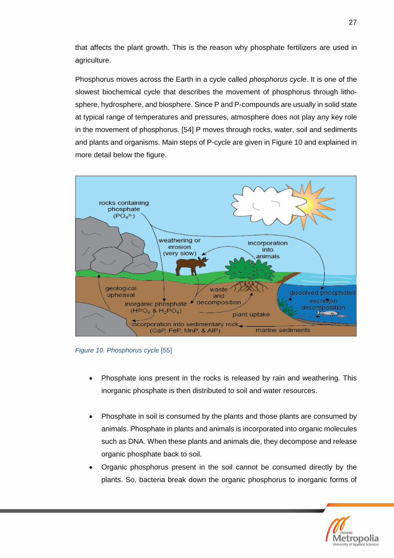
Phosphorus moves across the Earth in a cycle called phosphorus cycle. It is one of the
slowest biochemical cycle that describes the movement of phosphorus through litho-
sphere, hydrosphere, and biosphere. Since P and P-compounds are usually in solid state
at typical range of temperatures and pressures, atmosphere does not play any key role
in the movement of phosphorus. [54] P moves through rocks, water, soil and sediments
and plants and organisms. Main steps of P-cycle are given in Figure 10 and explained in
more detail below the figure.
Figure 10. Phosphorus cycle [55]
• Phosphate ions present in the rocks is released by rain and weathering. This
inorganic phosphate is then distributed to soil and water resources.
• Phosphate in soil is consumed by the plants and those plants are consumed by
animals. Phosphate in plants and animals is incorporated into organic molecules
such as DNA. When these plants and animals die, they decompose and release
organic phosphate back to soil.
• Organic phosphorus present in the soil cannot be consumed directly by the
plants. So, bacteria break down the organic phosphorus to inorganic forms of

28
phosphorus which can be easily consumed by the plants. This process is known
as mineralization.
• Phosphorus in the soil can end up in waterways, for instance, rivers and streams
through soil erosion and floods. Phosphorus present in these waterways finally
end up in oceans which is incorporated into sediments over time. P cycle have
significant impact of human activities. [51]
Sources of nutrients
Sources of nutrients discharge in the water bodies can be divided into two categories,
point source and nonpoint source. The major nonpoint sources of nutrient pollution in the
water bodies are excess fertilizers from agricultural land, livestock and pet wastes, for-
estry, natural background and atmospheric deposition of nutrients. Similarly, point
sources of nutrients pollution include sources such as effluent from wastewater treatment
plants, industry, and fish farming. [56]
In Finland, nutrients pollution from industries are under control but the nutrient loads
coming from agriculture are still significant accounting for up to 80% loads in some place.
Municipal wastewater treatment plants have been successful in removing the phospho-
rus effectively from wastewater but the level of nitrogen removal is still not good. Alt-
hough the farmers are given agri-environmental subsidies, the concentration of nutrient
loads in water is improving slowly. The main reason behind increase in nutrients in the
water from the agriculture has been climatic trends such as increase in winter rainfall,
frequent snowmelt and shorter duration of snow cover which has caused nutrients to
leach from agricultural fields more frequently. [57]
Figure 11. P and N discharges into surface waters from point sources in Finland (1980-2015) [57]

29
In Figure 11, we can see that the nutrients from point sources, industry and fish farming
has been decreasing with time and the limit for the removal of nutrients from wastewater
treatment plants set by EU Waste Water Directive has been widely achieved but the
nitrogen load in municipal wastewater has not been decreasing significantly.
Effect of nutrients
The main effect of overnutrition in the water bodies is eutrophication. It is the excessive
growth of plants and algae due to the increase in the nutrients along with other factors,
for example, sunlight and CO2 needed for photosynthesis. Eutrophication can occur nat-
urally over centuries and human activities have increased the rate of eutrophication
through different point and nonpoint sources of nutrients loading. This kind of eutrophi-
cation caused by an increase in limiting nutrients such as nitrogen and phosphorus is
known as cultural eutrophication. The consequences of cultural eutrophication are algal
blooms, contamination of drinking water and degradation of recreational activities. In US,
the cost of damage caused by eutrophication problem alone is approximately $2.2 billion
per year. The main effect of cultural eutrophication in water bodies is formation of toxic
and bad smelling phytoplankton that reduce the clarity of water and affect the water qual-
ity. Frequent rate of photosynthesis linked to eutrophication can cause depletion of dis-
solved inorganic carbon and raise the pH to extreme levels during day. Since some or-
ganisms depend on perception of dissolved chemical signals for their survival from pred-
ators, extreme pH can make them blind. Eutrophication results in algal blooms that limit
the penetration of light needed for photosynthesis that reduce the growth of plants and
affect predators that need light to catch their prey. When dense algal blooms die, the
process of microbial decomposition can use up all the available oxygen in the water
creating anoxic or dead zone. Lack of enough dissolved oxygen in the water bodies affect
the respiration of plants and aquatic organisms such as fishes and crabs that result in
death of those organisms. Some algae are toxic in nature as they produce toxins such
as microcystin and anatoxin. Algal blooms have ecological, social and economic impact.
Harmful algal blooms can degrade water quality, destruct economically important fisher-
ies, degrade recreation, tourism and pose public health risks in freshwater ecosystems.
[58]
Eutrophication has been a problem not only in rivers and lakes but its negative impacts
have been seen in marine ecosystem as well. Eutrophication is persistent problem in
one of the polluted sea, Baltic Sea. Agriculture is a major source of nutrients such as
phosphorus and nitrogen causing eutrophication in Baltic Sea. [59] In Finland, majority

30
of rivers are in coastal areas that contain excessive amounts of nutrient loads from agri-
cultural land. These rivers finally discharge nutrients into the Baltic Sea, either into the
Gulf of Finland or the Gulf of Bothnia. [60] Total discharge of nutrients, phosphorus and
nitrogen from Finnish rivers into Baltic Sea from 1970 to 2015 can be seen below in
Figure 12.
Figure 12. Total P and N discharge from Finnish rivers into Baltic Sea (1979-2015) [57]
Phosphorus and nitrogen load enter the Baltic Sea through rivers, and the amount of
load depends on weather conditions and with water volumes in the river. More nutrients
get into Baltic Sea during the year with high precipitation than in dry years. We can see
that nutrient discharge has increased since 2000 which is because of mild winter condi-
tions where the duration of snow cover is less. In case of nitrogen, mild winters speed
up the decomposition of organic material that increase the leaching of organic nitrogen
from the soils. [57]

31
3 MATERIALS AND METHODOLOGY
Both onsite measurements and laboratory measurements were performed to determine
the values for different parameters of water quality. Water quality parameters such as
turbidity, total iron, total nitrogen and total phosphorus were determined through labora-
tory measurements, whereas parameters such as sample depth, temperature, pH, elec-
trical conductivity and dissolved oxygen were measured onsite using different equip-
ment.
3.1 Sampling sites and conditions
Water samples for laboratory measurements were taken on 17.10.2016 and 18.10.2017
for the streams, Mätäjoki and Haaganpuro, respectively. Five sampling sites were cho-
sen for each stream. Sampling was done by grab methodology where samples were
collected only once at a time. From each stream five water samples were collected in
five 250 ml plastic bottles from different sites.
Onsite measurements were carried out on the same day of sampling, on 17.10.2016 and
18.10.2017 for Mätäjoki and Haaganpuro respectively. From each sampling sites, onsite
measurement was done thrice to obtain the mean value for the parameters.
Different sites, their location and sampling time for both streams can be seen below.
Table 3. Sampling sites, their location and sampling time for Mätäjoki
Sites Sampling
Time
Address Coordinates
M1 13:05 Solkikuja 8, 01600 Vantaa N 60O15’29.304’’ E
24O51’44.8308’’
M2 13:43 Gamla Nurminjärvivägen 3,
00420 Helsinki
N 60O15’8.4348’’ E
24O52’6.4704’’
M3 14:30 Fagottipolku 2, 00420 Helsinki N 60O14’24.072’’ E
24O51’49.392’’
M4 14:51 Trumpettipolun kevyen
liikenteen silta, 00420 Helsinki
N 60O14’16.0692’’ E
24O51’56.7972’’
M5 15:13 Mätäjoen kevyenliikenteen silta,
00440, Helsinki
N 60O14’5.0892’’ E
24O51’59.8752’’

32
Figure 13. Sampling sites of Mätäjoki
Table 4. Sampling sites, their location and sampling time for Haaganpuro
Sites Sampling
Time
Address Coordinates
H1 11:50 Hämeenlinnanväylä, 00101,
Helsinki
N 60O12’42.894’’ E
24O54’2.1492’’
H2 12:15 Hämeenlinnanväylä, 00101,
Helsinki
N 60O12’34.6428’’ E
24O53’52.1016’’
H3 12:41 Kytösuon kevyen liikenteen
silta, 00300, Helsinki
N 60O12’24.6816’’ E
24O53’38.3496’’
H4 13:05 Rymättylänpolku 2, 00300,
Helsinki
N 60O12’14.76’’ E
24O53’32.7588’’
H5 13:26 Tilkantorin kevyen liikenteen
silta, 00300, Helsinki
N 60O12’10.1844’’ E
24O53’30.9876’’

33
Figure 14. Sampling sites of Haaganpuro
3.1.1 Weather
The surrounding temperature was around 6-7 degree Celsius on both days, 17.10.2017
and 18.10.2017 during onsite measurements and sampling. In the first sampling day,
there was intermittent clouds, whereas second day was partly sunny. Probability of pre-
cipitation was 0%, humidity was 76% and cloud cover was 69% on first day of sampling,
whereas in second day of sampling it was 1%, 72% and 65% respectively.
3.1.2 Equipment used
The equipment used during sampling and onsite measurements are as follows:
• Sampling bottles
• Sample collector
• Depth measuring rod
• pH and conductivity meter (SevenGo DuoTM)
• DO meter (HQ40d)

34
3.1.3 Sampling procedures
Following procedures were applied before and during sampling:
• Before going to sampling sites, all the necessary equipment needed for sampling
were collected.
• Proper labeling of sampling bottles was done.
• Sample was collected directly from the sampling bottles except in some deep
sampling site, sample collector was used from the bridge to collect the sample.
• Sample bottles were rinsed more than 3 times before taking the sample.
• Samples were collected especially from the middle part of the stream where there
was a good flow.
• Lid of the sample bottles were closed air tight immediately after filling with water
sample to protect the sample from contaminations.
• After sample collection, sample bottles were kept in the refrigerator in Chemistry
laboratory of Metropolia UAS for preservation.
• Those samples were later used for the laboratory analysis.
3.2 Onsite measurements
3.2.1 Procedures
Before onsite measurements all necessary equipment were collected and different other
procedures were applied during onsite measurements which are as follows:
Sample depth
Depth of water was measured from the place where the sample was taken. Water depth
was measured using measuring rod. In the small water streams, depth was measured
easily, whereas in the deeper sampling site, measuring rod was used from the bridge.
pH and electrical conductivity
pH and electrical conductivity were measured using the pH meter. Before using the avail-
able pH meter, it was first calibrated. For the calibration of the pH meter, 3-point calibra-
tion was done with following steps:

35
• First, pH mode was selected and the electrode was rinsed with deionized water
and was dried using tissue paper.
• Electrode was then placed into the buffer solution of pH 4.01 and button ‘Cal ‘was
pressed and finally button ‘read ‘was pressed that displayed the buffer value 4.01.
• Similarly, the electrode was rinsed again with deionized water and was dried.
Then it was placed in next calibration buffer solution of pH 7 and button ‘Cal’ was
pressed and finally button ‘read’ was pressed that displayed the buffer value 7.
• As a last step, same above step was repeated using the buffer solution of 9.21.
Similarly, calibrated conductivity meter was used to measure the electrical conductivity
of water samples. During onsite measurements, pH/conductivity meter was dipped into
the water and button read was pressed and waited until the stable value was obtained
on the screen of pH/conductivity meter. The obtained stable values for pH and conduc-
tivity were noted. Before every new measurement, probe of pH/conductivity meter were
rinsed properly.
Dissolved oxygen and temperature
Dissolved oxygen (DO) and temperature were measured using a DO meter, HQ40d. The
measurement range of this equipment is 0.01-20 mg/l. The DO meter available in the
Environmental Engineering laboratory of Metropolia UAS was already calibrated. During
onsite measurements, the DO meter was dipped into the water and the Read button was
pressed. When the measurement was stable, a lock icon was shown on the screen. The
stable values of DO and temperature were noted down. For every new measurement,
the probe of DO meter was rinsed properly.
3.3 Laboratory measurements
Laboratory measurements were carried out in the Environmental Engineering laboratory
of Metropolia UAS. Equipment used and procedures applied during laboratory works are
as follows:
3.3.1 Equipment used
Equipment used during laboratory measurements are the following:
• Hanna HI 88713- ISO Turbidity meter
• Hach/Lange Spectrophotometer DR 3900

36
• Hach/Lange LT200 Thermostat
• Microwave Plasma – Atomic Emission Spectroscopy (4100 MP-AES)
• Round bottom flasks of different sizes
• Beakers
• Filter Papers
• Pipette
3.3.2 Chemicals used
Chemicals used during laboratory measurements are listed below:
• Reagents used in analysis of nitrogen and phosphorus (LCK 138 and LCK 349)
• (Fe2+ 200 mg/l + 2 ml 2.5 M H2SO4) solution
3.3.3 Procedures
Procedures used for different laboratory measurements are explained in the following
paragraphs.
Turbidity
Turbidity was measured using turbidity meter in Environmental Engineering lab. When
taking the measurements, cuvettes without any scratches were used to prevent inaccu-
rate readings. Around 10 ml of water sample was filled in the dry and clean cuvettes and
were properly capped to prevent spillage of water samples. Cuvette was wiped with lint-
free cloth adding few drops of silicon oil to obtain accurate readings. Then the sample
containing cuvette was placed into the turbidity meter and the lid was closed. ’Read’
button was pressed to obtain the value of turbidity in selected units. Obtained values
were noted down for analysis.
Total iron
Total iron concentration of water samples was measured using Agilent 4100 MP-AES.
In the beginning, colorimetric analysis was chosen to determine the iron concentration in
the water samples which is based on the change in the intensity of color of solutions with
variations in concentrations. But even with adding reagents, hydroxylamine hydrochlo-

37
ride and o-phenanthroline solution, samples did not show any color as they were sup-
posed to like the standard solutions with concentrations 0.5 to 5 mg/l. Hydroxylamine
hydrochloride is a reducing agent that takes iron present in the solution from 3+ oxidation
state down to 2+ oxidation state and o-phenanthroline is a reagent that react with iron in
2+ oxidation state to form a color complex. No change in color, proved that the concen-
tration of iron in the water sample was very low below 0.5 mg/l.
To find out the exact concentration of iron in the water samples, even the concentration
was below 0.5 mg/l, 4100 MP-AES technology was used. 4100 MP-AES uses microwave
plasma and an atomic emission spectroscopy detector which is a new and enhanced
technology in the field of environmental monitoring and analysis. MP-AES is similar to
Induced Couple Plasma – Atomic Emission Spectroscopy (ICP-AES) as they both meas-
ure and analyze spectra by an atomic emission spectrometer (AES) using concentration-
intensity correlations which are similar to how Beer-Lambert law applies to atomic ab-
sorption spectroscopy (AAS). [61]
The difference between MP-AES and ICP-AES is the way how the plasma is formed.
4100 MP-AES uses nitrogen based plasma that runs on air using N2 generator, that gives
strong plasma and conventional torch. Nitrogen based plasma reaches temperature of
approximately 5000 K. At such a temperature, atomic emission is strong producing ex-
cellent detection limits. [62] Instrument uses atomic emission detection at predefined
wavelength. [63] It has higher improved performance than flame atomic absorption (AA).
It is cost effective since it runs on air, there is no need of expensive gas such as argon.
It is easy to use and has improved safety as it eliminates use of flammable gases. [64]
Working principle of MP-AES
Inside MP-AES instrument, plasma is formed in a conventional torch using nitrogen gas.
This formed plasma is a high temperature excitation source which is ideal for the sample
atomization and excitation producing high intensity emission lines. First, aerosols formed
from sample using nebulizer and spray-chamber goes into the plasma where they are
dried, decomposed and atomized. Once an atom is excited it emits light in a character-
istic pattern of wavelengths (emission spectrum) as it returns to the lower energy states.
Emission from the plasma is then directed into fast scanning monochromator. The se-
lected wavelength range is imaged onto the high efficiency CCD detector that measures
both spectra and background simultaneously for optical precision. MP-AES then meas-
ure the quantity of concentration of an element in a sample by comparing its emission to
that of known concentrations of the element which is plotted on a calibration curve. The
final result obtained is the concentration of element in the sample. [62]

38
Figure 15. Iron test using 4100 MP-AES technology
Preparation and measurement of standard solutions and unknown samples
Six standard solutions of concentrations (M2), 0.05, 0.15, 0.25, 0.35, 0.45 and 0.50 ppm
were prepared using available (Fe2+ 200 mg/l + 2 ml 2.5 M H2SO4) mother solution. Di-
lution of mother solution was done in such a way that volume of solution to be pipette
lies in between 0.5 ml to 5 ml to prepare standard solutions. Therefore, for the dilution,
5 ml of mother solution was added to a flask of 100 ml (V2), which was then filled with
deionized water till the mark. The concentration of the mother solution (M1) became 10
ppm. The volume of mother solution (V1) to be pipetted in six different 100 ml flasks, was
calculated as 0.5, 1.5, 2.5, 3.5, 4.5 and 5 ml, using the formula, M1*V1=M2*V2. After
pipetting respective volume of solutions, flasks were filled with deionized water till the
mark. In this way six standard solution of known concentrations were prepared to make
the calibration curve.
Ten unknown samples of ten different sites of two streams were first filtered using filter
paper to remove the suspended solid particles in the water sample. 50 ml of each filtered
samples were put into flasks for the measurement.
After preparing standard solutions and unknown samples, calibration curve was plotted
using known concentrations of standard solutions in the computer connected with MP-
AES machine. Then unknown samples were measured one by one using MP-AES. Fi-
nally, the concentrations of all unknown samples were obtained in the computer.

39
Nitrogen and phosphorus
Total nitrogen and phosphorus were measured using Hach/Lange Spectrophotometer
DR 3900 (Figure 16). DR 3900 is UV/Visible spectrophotometer with a wavelength of
320-1100 nm. It works on the principle that the concentration of the substances to be
analyzed is determined when the light is absorbed by the sample at the certain wave-
length. It is one of the easiest way to perform test for the water analysis that provides
digital readouts in the units of concentration, absorbance or percent transmittance. Ni-
trogen and phosphorus test have separate ways of preparing sample. [65]
Water samples were taken out from the refrigerator and all the necessary kits were made
ready for the evaluation of total nitrogen and phosphorus in the water samples. The sam-
ple preparation and measurement procedure for total nitrogen and total phosphorus are
explained, respectively, in the following paragraphs.
Figure 16. Nitrogen and phosphorus test using Hach/Lange Spectrophotometer DR 3900
Datasheet of product LCK138 was used to follow the procedures of sample preparation
and measurement for total nitrogen in the sample. The measuring range is 1-16 mg/L
TNb. First, 1.3 ml of the water sample, 1.3 ml of the solution Reagent A and 1 tablet of
Reagent B were added in quick succession to a dry reaction tube and it was closed
immediately without inverting. Then, the reaction tube was heated immediately at the
temperature of 100 OC for 60 minutes in the thermostat. After that, it was cooled down,
and 1 MicroCap of reagent C was added. The reaction tube was closed and inverted a

40
few times until the freeze-dried contents were fully removed from the MicroCap C and all
streaks were vanished. Next, 0.5 ml of digested sample was pipetted slowly into the
cuvette test, after which 0.2 ml of Solution D was slowly pipetted in the cuvette and it
was immediately closed and inverted a few times until no more streaks were seen. Fi-
nally, after 15 minutes, the outside part of cuvette was cleaned thoroughly, and the cu-
vette was inserted in DR 3900 spectrophotometer to evaluate the concentration of nitro-
gen in the sample.
Datasheet of product LCK349 was used to follow the procedures of sample preparation
and measurement for total Phosphorus in sample. The measuring range is 0.05-1.5 mg/l
PO4-4. First, the foil was removed carefully from the screwed-on DosiCap Zip. DosiCap
Zip was unscrewed and 2.0 ml of sample was pipetted into the cuvette. DosiCap Zip was
then screwed back tightly keeping the fluting at the top. The cuvette was shaken firmly
back and forth 2 to 3 times. Next, it was heated in the thermostat at the temperature of
100 OC for around 60 minutes. It was allowed to cool at room temperature and was
shaken firmly. After that, 0.2 ml of Reagent B was pipetted into the cooled cuvette. Rea-
gent B was closed immediately after use. Grey DosiCap C was then screwed onto the
cuvette and it was inverted few times. The cuvette was left in room temperature for 10
minutes and was inverted few times more. Finally, the outer part of the cuvette was
cleaned thoroughly, and the cuvette was inserted in DR 3900 spectrophotometer to eval-
uate the concentration of phosphorus in the sample.
3.4 Safety precautions
Safety measures were applied while performing water sampling, onsite measurements
and laboratory analysis. During water sampling and onsite measurements, priority was
given to safety measures such as use of gloves, proper clothes and shoes. In the larger
and deeper sampling sites, sample was taken from the bridge using a water sample
collector.
In the laboratory measurements, priority was given to chemical safety. Chemical rea-
gents used in iron, nitrogen and phosphorus measurements are corrosive, hazardous to
health, irritating and poisonous. Therefore, safety measures such as wearing gloves, lab
coats and safety glasses were applied to protect skin and eyes. Safety data sheet of
reagents of products LCK 138 and LCK 349 were read before handling any chemicals
during laboratory works.

41
4 RESULTS
The results of parameters obtained from different onsite measurements and laboratory
measurements of the streams Mätäjoki and Haaganpuro are presented in two sections
labeled according to the names of the streams.
4.1 Mätäjoki
The results obtained from onsite measurements for stream Mätäjoki were as follows:
Table 5. Results of onsite measurements of Mätäjoki
Samples Sample
Depth
(cm)
pH Conductivity
(µS/cm)
Temperature
(OC)
Dissolved
Oxygen
(mg/l)
Oxygen
Saturation
(%)
6.93 322 7.1 2.01 16.2
M1 46 6.98 365 6.9 1.57 13.0
7.06 329 6.9 1.41 11.3
7.14 325 6.0 2.91 22.8
M2 16 7.17 332 6.1 2.36 18.5
7.19 331 6.1 2.69 21.1
7.35 370 5.7 8.60 66.8
M3 80 7.56 373 5.5 8.84 68.3
7.50 371 6.0 8.46 66.2
7.51 341 5.5 7.20 55.6
M4 35 7.47 346 5.6 7.02 54.2
7.49 348 5.5 6.93 53.5
7.59 338 5.9 6.63 51.7
M5 31.5 7.66 346 5.7 6.77 52.6
7.65 249 5.6 6.99 54.2

42
In Mätäjoki, sampling and onsite measurements were done from the sites having water
depth between 0.1 to 0.8 m. Three measurements were done for different parameters
from each sampling sites. The average water temperature of the stream was 6.0 OC with
pH in the range of 7 to 8. The concentration of DO varied from 1 to 9 mg/l with average
oxygen saturation of 40%. Sampling sites, M1 and M2 had very low level of DO in com-
parison to other sites. The average electrical conductivity of stream was around 340
µS/cm.
The results obtained from laboratory measurements were as follows:
Table 6. Results of laboratory measurements of Mätäjoki
Site NTotal (mg/l) PTotal (mg/l) FeTotal (mg/l) Turbidity
(NTU)
M1 1.17 0.080 0.36 5.51
M2 1.31 0.095 0.33 6.06
M3 1.31 0.045 * 0.33 6.36
M4 1.45 0.075 0.43 5.97
M5 1.29 0.059 0.32 * 6.77
In Mätäjoki the concentration of total nitrogen and phosphorus was very low. The aver-
age total nitrogen concentration in the stream was 1.3 mg/l, whereas the average con-
centration of total phosphorus was 0.07 mg/l. In site M3, the concentration of total phos-
phorus was below the measuring range as the total phosphorus was measured in the
range of 0.05-1.5 mg/l.
The average total iron in the stream was 0.35 mg/l. In site M5, the actual concentration
of total iron was 0.64 mg/l which was out of measuring range; thus, it was diluted by a
dilution factor of 2, to get the value within the measuring range. The average turbidity of
Mätäjoki was 6.0 NTU.
4.2 Haaganpuro
The results obtained from onsite measurements for stream Haaganpuro were as follows:

43
Table 7. Results of onsite measurements of Haaganpuro
Samples Sample
Depth
(cm)
pH Conductivity
(µS/cm)
Temperature
(OC)
Dissolved
Oxygen
(mg/l)
Oxygen
Saturation
(%)
7.42 388 7.3 10.81 87.9
H1 17 7.61 395 7.0 10.97 88.4
7.70 396 6.8 10.96 87.9
7.51 403 7.3 10.41 85.0
H2 42 7.61 408 7.1 10.49 84.7
7.67 409 7.0 10.51 84.7
7.58 404 7.3 9.70 78.9
H3 26 7.63 411 7.1 9.86 79.7
7.69 412 7.1 9.87 79.8
7.76 416 6.8 8.01 64.2
H4 28 7.73 422 6.5 8.03 63.9
7.72 425 6.5 8.02 63.8
7.70 406 6.8 8.57 68.6
H5 30 7.69 411 6.6 8.61 68.7
7.67 413 6.5 8.43 67.1
In Haaganpuro, sampling and onsite measurements were done from the sites having
water depth between 0.1 to 0.42 m. Three measurements were done for different param-
eters from each sampling sites. The average water temperature of the stream was 7.0
OC with average pH of 7.6. The concentration of DO varied from 8 to 11 mg/l with average
oxygen saturation of 77%. All the sampling sites had similar concentrations of DO. The
average electrical conductivity of the stream was around 408 µS/cm.
The results obtained from laboratory measurements were as follows:

44
Table 8. Results of laboratory measurements of Haaganpuro
Site NTotal (mg/l) PTotal (mg/l) FeTotal (mg/l) Turbidity
(NTU)
H1 0.61 0.037 * 0.33 6.10
H2 1.46 0.017 * 0.28 7.24
H3 0.58 0.033 * 0.24 5.90
H4 1.55 0.037 * 0.19 8.67
H5 1.07 0.044 * 0.29 6.30
In Haaganpuro, the concentration of total nitrogen and phosphorus was very low. The
average total nitrogen concentration in the stream was 1.05 mg/l, whereas the average
concentration of total phosphorus was 0.03 mg/l. The concentration of total nitrogen in
the sites H1 and H3 was under the measuring range, whereas the concentration of total
phosphorus in all the sites was under the measuring range as the total phosphorus was
measured in the range of 0.05-1.5 mg/l. The average total iron concentration and aver-
age turbidity in the stream was 0.27 mg/l and 6.0 NTU respectively.
5 DISCUSSION
This section discusses the results of water quality parameters for the streams, Mätäjoki
and Haaganpuro obtained from both onsite measurements and laboratory evaluations.
5.1 Mätäjoki VS Haaganpuro
The water quality of Mätäjoki seems good based on the chosen physio-chemical param-
eters and sampling season. pH of water in Mätäjoki during autumn 2016 was in the range
suitable for the aquatic life, since the normal range of pH in freshwaters is 6.5 to 9. The
water temperature of Mätäjoki is in the optimal range needed for trout. The minimum
concentration of DO in streams to support large species of fishes is 4 mg/l. Result shows
that sites M1 and M2 have very low level of DO which is below the minimum level needed
for aquatic life. The main reason behind the low level of DO in these sites can be over
growth of plant species, bacteria and excess DO that consume more oxygen and the

45
increase in the number of cloudy days that make respiring plants to use more oxygen
because of no photosynthesis. [23] Mätäjoki has an optimum electrical conductivity that
lies in the range of 150-500 µS/cm that support the diverse aquatic life. [66] The turbidity
level in Mätäjoki is below 7 NTU, which shows that it does not have any effect on aquatic
life, especially trout. The acceptable range of turbidity for trout streams is less than 10
NTU. [67] The level of nutrients and iron concentration seems fine in Mätäjoki. For rivers
and streams to be eutrophic, the suggested limit of total nitrogen is >1.5 mg/l, whereas
for total phosphorus it is >0.075 mg/l. Both nutrients in Mätäjoki are within the limit; how-
ever, the concentration of total phosphorus seems very close to the limit value that can
cause eutrophication in the stream. The main source of phosphorus in the streams, for
example, Mätäjoki in Finland is agricultural discharge and effluent from the paper and
pulp industries. [68]
The quality of water in Haaganpuro also seems pretty fine based on chosen water quality
parameters and sampling season. Water temperature, pH, conductivity, DO and turbidity
level of Haaganpuro is in the range that supports aquatic life. Similarly, the results show
that the concentrations of nutrients and total iron in the water is very low.
The quality of water in both streams are good and within the standard limits, but if we
compare the water quality of these streams, Haaganpuro is little better than Mätäjoki.
They are similar in terms of water temperature, pH, conductivity, and turbidity. The level
of DO in Haaganpuro is far better than in Mätäjoki that means aquatic life is better in
Haaganpuro. Similarly, in terms of nutrients and total iron concentration, Haaganpuro
seems better.
5.2 Water quality of Mätäjoki (1995-2016)
Water quality monitoring of Mätäjoki started from 1987 by Environmental Center, city of
Helsinki. Water quality of Mätäjoki was studied in detail by Olli Ruth in the year 1995-
1996 where the samples were taken at weekly intervals. Precipitation during the moni-
toring period was less than normal which was about 85% of a normal year and its flow
into the bay of Iso-Huopalahti was 140 l/s. The average water temperature during the
year was 6.4 OC. During the year, the median water pH at various sampling points was
7.1. The water quality of Mätäjoki was in better condition than in mid 1970s. [4]
In 2004, water quality of Mätäjoki was monitored along with other 21 urban streams in
Helsinki by Vuokko Tarvainen. The average water temperature of the stream was 7.12
OC. The pH of the runoff water was on average of 7.18. The average saturation rate for

46
the whole brook was 64%. Regarding other variables, there were no special problems
with water quality. [69]
Results from onsite and laboratory measurements of 2016 show that there are changes
in water quality parameters in Mätäjoki from 1995 to 2016 (Figure 17, Figure 18 and
Figure 19).
Figure 17. Electrical conductivity in Mätäjoki (1995-2016)
The electrical conductivity of the various sampling points in the runway varied very much
in the same way as the dissolved substance concentration in 1995-1996. Conductivity
was smallest in the upper stream at Vantaa and increased in the lower stream near the
sea. The average conductivity of all sampling points was 677 µS/cm. [4] The conductivity
of Mätäjoki in 2004 was in the range of 139 to 683 µS/cm. [69] In Figure 17, we can see
that the conductivity of Mätäjoki in 2016 has decreased by almost half than in 1995-1196
and is slightly higher than it was in 2004.
0
100
200
300
400
500
600
700
800
1995-1996 2004 2016
µS
/cm
Year

47
Figure 18. DO and turbidity level in Mätäjoki (1995-2016)
The oxygen content of the water fluctuated from 0.1mg/l to 14.1 mg/l during the year
1995-1996 from samples collected at different sampling points. Oxygen saturation in the
stream varied from 1-97 % during individual observations. The average oxygen satura-
tion was 61 % and average turbidity was 26 FTU. [4] In 2004, concentration of dissolved
oxygen varied from 2.41 to 13.25 mg/l and turbidity was in the range of 4.8-36 NTU. [69]
Change in the concentration of dissolved oxygen and the level of turbidity from 1995-
1996 to 2016 can be seen in Figure 18. Level of DO is low in Mätäjoki in 2016 than it
was in 1995-1996 and 2004, and the turbidity level is excellent in 2016 in comparison to
years, 1995-1996 and 2004 (Figure 18).
Figure 19. Total N and Total P concentration in Mätäjoki (1995-2016)
0
5
10
15
20
25
30
0
1
2
3
4
5
6
7
8
9
1995-1996 2004 2016
Tu
rbid
ity(N
TU
)
Dis
so
lve
d O
xyg
en
(m
g/l
)
Year
Dissolved Oxygen Turbidity
0
10
20
30
40
50
60
70
80
0
0.2
0.4
0.6
0.8
1
1.2
1.4
1.6
1.8
1995-1996 2004 2016
Year
To
tal P
ho
sp
ho
rus
(μ
g/l
)
To
tal N
itro
ge
n (
mg
/l)
Nutrients
Total Nitrogen Total Phosphorus

48
In 1995-1996, total nitrogen concentration varied from 0.92 to 3.8 mg/l and total phos-
phorus varied from 0.017 to 0.13 mg/l. On average, 50% of total nitrogen was NO3, 22.5
% was NH4 and 1.2% was NO2. [4] Similarly, in 2004 the concentration of total nitrogen
was in the range of 0.57 to 3.3 mg/l and total phosphorus was in the range of 0.014 to
0.095 mg/l. [69] Change in the average concentration of both nutrients from 1995-1996
to 2016 can be seen in Figure 19. Total nitrogen in Mätäjoki has decreased in 2016,
whereas total phosphorus has increased (Figure 19).
The concentration of total iron in Mätäjoki is better than it was in 1995-1996. In the year
1995-1996, water contained an average of 1.4mg/l of iron in the entire stream. Between
1979 and 1989, samples taken at various runoffs contain an average of 2.6 mg/l of iron.
[4] Present total iron concentration in Mätäjoki which is below 0.4 mg/l shows that con-
centration of iron in the stream is in better condition.
5.3 Water quality of Haaganpuro (1987-2016)
Water quality monitoring of Haaganpuro started from 1987 by Environmental Center, city
of Helsinki. Two annual water samples from summer and autumn were taken from Haa-
ganpuro to monitor the water quality. The average water temperature between July and
October was 10.8 OC with average pH of 7.35. [70]
According to the water quality monitoring done by Vuokko Tarvainen in 2004, the water
quality of Haaganpuro was fairly good. The average water temperature was 6.6 OC with
average pH 7.29. [69]
Results from onsite and laboratory measurements of 2016 show that there are changes
in water quality parameters in Haaganpuro from 1987 to 2016 (Figure 20, Figure 21 and
Figure 22).

49
Figure 20. Electrical conductivity in Haaganpuro (1987-2016)
In Figure 20, we can see that the average conductivity of Haaganpuro in 2016 is greater
than it was in 1987 and 2004. Conductivity was least in the year 2004 in comparison to
1987 and 2016.
Figure 21. DO and turbidity level in Haaganpuro (1987-2016)
300
320
340
360
380
400
420
1987 2004 2016
μS
/cm
Year
0
5
10
15
20
25
30
35
40
45
8.6
8.8
9
9.2
9.4
9.6
9.8
10
1987 2004 2016
Tu
rbid
ity (
NT
U)
Dis
so
lve
d O
xyg
en
(m
g/l
)
Year
Dissolved Oxygen Turbidity

50
In 1987, DO in Haaganpuro was 9.0 mg/l in the month of July and 10.7 mg/l in October.
The average oxygen saturation was 86.5 %. [70] In 2004, Haaganpuro had average ox-
ygen saturation of 73.3%. [69] Turbidity level was higher in 1987 than in the year 2004.
Change in the concentration of dissolved oxygen and the level of turbidity from 1987 to
2016 can be seen in Figure 21. The level of DO in Haaganpuro in 2016 is greater than it
was in 2004 and the level of turbidity has decreased significantly from 1987 to 2016
(Figure 21).
Figure 22. Total N and Total P concentration in Haaganpuro (1987-2016)
In 1987 the concentration of total nitrogen was 1.6 mg/l in the month of July and it was
1.4 mg/l in October. The concentration of total phosphorus was found to be same in July
and October. [70] In 2004, total nitrogen was in the range of 0.83 to 2.2 mg/l, whereas
total phosphorus was in the range of 11 to 118 μg/l. [69] The change in the average
concentration of both nutrients from 1987 to 2016 can be seen in Figure 22. Concentra-
tion of both total nitrogen and total phosphorus in Haaganpuro is better in 2016 than in
1987 and 2004.
The concentration of total iron in Haaganpuro is better than it was in 1987. In the year
1987, water contained an average of 3.0 mg/l of iron in the stream. [70] The average
concentration of total iron was found to be 2.85 mg/l in 2004. [69] Present total iron con-
centration in Haaganpuro which is below 0.3 mg/l shows that concentration of iron in the
stream has decreased drastically.
0
20
40
60
80
100
120
0
0.2
0.4
0.6
0.8
1
1.2
1.4
1.6
1.8
1987 2004 2016
Year
To
tal P
ho
sp
ho
rus
(μ
g/l
)
To
tal N
itro
ge
n (
mg
/l)
Nutrients
Total Nitrogen Total Phosphorus

51
6 CONCLUSION
The main goal of this thesis was to study the quality of water in urban streams, Mätäjoki
and Haaganpuro. Results of onsite measurements and laboratory measurements show
that the water quality in both streams is in good condition. Almost all the water quality
parameters are within the limit to support the aquatic life in these streams. The compar-
ison of water quality parameters of these streams clearly shows that Haaganpuro is in
better condition than Mätäjoki. The problem found in the Mätäjoki is that, the concentra-
tion of dissolved oxygen in the first two sampling sites was too low to support aquatic
life. The average concentration of total phosphorus in Mätäjoki was found to be very
close to limit value that can support algal bloom in the stream.
Water quality of both Mätäjoki and Haaganpuro has been monitored for a long time.
Comparing three different years of data, water quality in both streams is in better condi-
tion than it was in the past. Turbidity and total iron concentration has decreased signifi-
cantly in both streams. Currently, total nitrogen in both streams is seen low than it was
in the past. Only the total phosphorus concentration has increased in Mätäjoki in com-
parison to past data, whereas in case of Haaganpuro, total phosphorus has decreased.
In general, therefore, it seems that sampling sites M1 and M2 of Mätäjoki having very
low DO have possibility that they have excess plants and bacteria that consume the
oxygen in the water. High concentration of total phosphorus in Mätäjoki suggests that
sources such as agriculture, pulp and paper industries and wastewater treatment plants
are still contributing phosphorus in the stream to some level. To maintain the good water
quality of these streams, it is important to reduce pollutants and nutrients loading from
both point and nonpoint sources.
This thesis provides the latest knowledge on the current situation of water quality in
Mätäjoki and Haaganpuro based on chosen parameters. A limitation of this study is that
samples were collected from only five sampling points for each stream and that they
were collected in a single day for each stream. More regular monitoring is needed to
determine the clear trend of water quality in these urban streams.

52
References
1. Fundamentals of Environmental Measures. [Internet]. Ohio: Fondriest Environ-
mental Inc.; (no date) Water Quality [cited 2017 Apr 3]. Available from:
http://www.fondriest.com/environmental-measurements/parameters/water-qual-
ity/
2. Virtavesien Hoitoyhdistys Ry. Mätäjoki [Internet]. Espoo: Virtavesien
Hoitoyhdistys Ry [Water Streams Management Association]; 2013 Dec 21 [cited
2017 Apr 3]. Available from: http://www.virtavesi.com/index.php?upper-
CatId=23&catid=44 [in Finnish]
3. Pajamäki seura ry. Mätäjoki [Internet]. Helsinki: Pajamäki seura ry [Pajamäki
Society]; (no date) [cited 2017 Apr 3]. Available from: http://xn--pajamki-
9wa.fi/pajamaki/lahiluonto/matajoki [in Finnish]
4. Ruth O. Mätäjoki- nimeään parempii [Mätäjoki- better than its name] [Internet].
Helsinki; Helsingin Kaupungin Ympäristökeskuksen Julkaisuja [City of Helsinki
Environment Center Publications]; 1998 [cited 2017 Apr 4]. Available from:
http://www.hel.fi/static/ymk/julkaisut/julkaisu-06-98.pdf) [in Finnish]
5. Saikku M. Mätäpuro [Internet]. Espoo: Virtavesien Hoitoyhdistys Ry [Water
Streams Management Association]; (no date) [cited 2017 Apr 3]. Available from:
(http://www.virtavesi.com/index.php?upperCatId=23&catid=24) [in Finnish]
6. Tuh. Urbaanit Taimenet [Urban Trouts] [Internet]. Finland: Geocaching; 2011
Nov 26 [cited 2017 Apr 3]. Available from: (https://www.geocaching.com/geo-
cache/GC36PDX_urbaanit-taimenet?guid=d908f786-6a30-46c3-9f76-
0888d5824fdf) [in Finnish]
7. River Restoration Center. Environmental History of the Mätäpuro Brook, Hel-
sinki, Finland [Internet]. River Restoration Centre; 2010 [cited 2017 Apr 4].
Available from: http://www.therrc.co.uk/pdf/conferences/Delegate_pack_10.pdf)
8. Teivainen A, Negligence caused toxic solvent leak, police conclude. Helsinki
Times. [Internet] 11 March 2014. [cited 2017 May 13]. Available from:

53
http://www.helsinkitimes.fi/finland/finland-news/domestic/9719-negligence-
caused-toxic-solvent-leak-police-conclude.html
9. Daniels M, Scott T, Haggard B, Sharpley A, Daniel T. What is Water Quality [In-
ternet]. Arkansas: University of Arkansas Cooperative Extension Service; (no
date) [cited 2017 Apr 4]. Available from: https://www.uaex.edu/publica-
tions/pdf/FSA-9528.pdf
10. Meybeck M, Kuusisto E, Mäkelä A, Mälkki E. Water Quality. In: Bartram J, Bal-
lance R, editors. Water Quality Monitoring - A Practical Guide to the Design and
Implementation of Freshwater Quality Studies and Monitoring Programmes [In-
ternet]. United Nations Environment Programme and the World Health Organi-
zation; 1996. Chapter 2. [cited 2017 Apr 4]. Available from:
(http://www.who.int/water_sanitation_health/resourcesquality/wqm-
chap2.pdf?ua=1)
11. Fundamentals of Environmental Measures [Internet]. Ohio: Fondriest Environ-
mental, Inc.; 7 February 2014. Water Temperature, [cited 2017 Apr 4]. Available
from: http://www.fondriest.com/environmental-measurements/parameters/wa-
ter-quality/water-temperature/
12. Fundamentals of Environmental Measurements [Internet]. Ohio: Fondriest Envi-
ronmental, Inc.; 2013 Nov 19. pH of Water. [cited 2017 Apr 5] Available
from: http://www.fondriest.com/environmental-measurements/parameters/wa-
ter-quality/ph/
13. The US Geological Survey’s Water Science School. pH- - Water Properties. [In-
ternet]. Virginia: USGS; (no date) [cited 2017 Apr 5]. Available from: https://wa-
ter.usgs.gov/edu/ph.html
14. Foo R. What factors can affect the pH of drinking water? [Internet]. Weebly; (no
date) [cited 2017 Apr 5]. Available from: http://endlead.weebly.com/factors-that-
affect-ph.html
15. Libretexts. Temperature Dependence of the pH of pure Water [Internet]. Califor-
nia: UCDAVIS; (no date) [cited 2017 Apr 5] Table 1, Effects of temperature on

54
Kw. Available from: https://chem.libretexts.org/Core/Physical_and_Theoreti-
cal_Chemistry/Acids_and_Bases/Acids_and_Bases_in_Aqueous_Solu-
tions/The_pH_Scale/Temperature_Dependence_of_the_pH_of_pure_Water
16. Fundamentals of Environmental Measurements [Internet]. Ohio: Fondriest Envi-
ronmental Inc; 3 March 2014. Conductivity, Salinity and Total Dissolved Solids.
[cited 2017 Apr 7]. Available from: http://www.fondriest.com/environmental-
measurements/parameters/water- quality/conductivity-salinity-tds/
17. Lenntech. Water Conductivity [Internet]. Rotterdamseweg: Lenntech; (no date)
[cited 2017 Apr 7.] Available from: http://www.lenntech.com/applications/ul-
trapure/conductivity/water-conductivity.htm
18. Player K, Bates H. Electrical Conductivity [Internet]. Sydney: Australian Mu-
seum; (no date) [updated 2015 Oct 7; cited 2017 June 10] Available from:
https://australianmuseum.net.au/electrical-conductivity
19. Baron J, Ashton C. The Effect of Temperature on Conductivity Measurement
[Internet]. Clare, Ireland: Reagecon Diagnostics Ltd; (no date) [cited 2017 Apr
7]. Available from: https://www.reagecon.com/pdf/technicalpapers/Ef-
fect_of_Temperature_TSP-07_Issue3.pdf
20. Zaidi J, Pal A. Influence of Temperature on Physico-Chemical Properties of
Freshwater ecosystem of Bundelkhand Region of Uttar Pradesh, India. Int. J.
Curr.Res.Chem.Pharma.Sci. [Internet]. 2015; 2(3): 1-8. [cited 2017 Apr 7].
Available from: http://www.ijcrcps.com/pdfcopy/mar2015/ijcrcps1.pdf
21. Sara. What is a solubility graph? [Internet]. Socratic; 2017 Jan 28. [cited 2017
Apr 7] Figure 1. Solubility Graph. Available from: https://socratic.org/ques-
tions/what-is-a-solubility-graph
22. Lenntech. Dissolved Oxygen [Internet]. Rotterdamseweg: Lenntech; (no date)
[cited 2017 Apr 8] Available from: http://www.lenntech.com/why_the_oxy-
gen_dissolved_is_important.htm
55
23. Oram B. Dissolved Oxygen in Water [Internet]. Dallas: BF Environmental Con-
sultants Inc.; (no date) [cited 2017 Apr 8] Available from: http://www.water-re-
search.net/index.php/dissovled-oxygen-in-water
24. Westminster College SIM. Temperature effects on Dissolved Oxygen in Water
[Internet]. Beaverton: Vernier Software and Technology; 2000 [cited 2017 Apr
8]. Table 1. Normal Tolerance of Selected Animals to Temperature and Oxygen
levels. Available from: http://www.westminster.edu/about/community/sim/docu-
ments/stemperatureeffectsondissolvedoxygeninwater-comp_000.pdf
25. Mesner N, Geiger J. Dissolved Oxygen [Internet]. Utah State University;(no
date);[reviewed 2010 December; cited 2017 Apr 8]. Available from: http://exten-
sion.usu.edu/waterquality/files-ou/whats-in-your-water/do/NR_WQ_2005-16dis-
solvedoxygen.pdf
26. Water Quality [Internet]. Utah State University; (no date). Dissolved Oxygen.
[cited 2017 Apr 8]. Available from: http://extension.usu.edu/waterquality/whats-
in-your-water/do
27. Murphy S. General information on Dissolved Oxygen [Internet]. Colorado: City
of Boulder; (no date) [updated 2007 Apr 23; cited 2017 Apr 8]. Available from:
http://bcn.boulder.co.us/basin/data/NEW/info/DO.html
28. Fundamentals of Environmental Measurements [Internet]. Ohio : Fondriest En-
vironmental, Inc. ; 2013 Nov 19. Dissolved Oxygen. [cited 2017 Apr 8]. Availa-
ble from: http://www.fondriest.com/environmental-measurements/parame-
ters/water-quality/dissolved-oxygen/
29. The US Geological Survey’s Water Science School. Turbidity [Internet]. Vir-
ginia: USGS; (no date) [cited 2017 Apr 11]. Available from: https://wa-
ter.usgs.gov/edu/turbidity.html
30. GB Waterwatch. Turbidity Information Sheet [Internet]. Goulbourn: GB Water-
watch; (no date). [cited 2017 Apr 11]. Available from: http://www.gbwater-
watch.org.au/resources/ID1297385597.pdf

56
31. Lenntech. Turbidity [Internet]. Rotterdamseweg: Lenntech; (no date). [cited
2017 Apr 11]. Available from: http://www.lenntech.com/turbid-
ity.htm#ixzz4dxLmUbvS
32. Vernier Software and Technology. Water Quality- Turbidity [Internet]. Beaver-
ton: Vernier Software and Technology; (no date) [cited 2017 Apr 11]. Available
from: http://www2.vernier.com/sample_labs/ESV-12-COMP-water_quality_tur-
bidity.pdf
33. Fundamentals of Environmental Measurements [Internet]. Ohio: Fondriest Envi-
ronmental, Inc.; 2014 June 13. Turbidity, Total Suspended Solids and Water
Clarity; [cited 2017 Apr 11]. Available from: http://www.fondriest.com/environ-
mental-measurements/parameters/water-quality/turbidity-total-suspended-sol-
ids-water-clarity/
34. Bronsdon R, Clark J, et al. Rivers and their catchments: causes and effects of
turbid water [Internet]. Scotland: Scottish National Heritage; (no date) [cited
2017 Apr 11]. Available from: http://www.snh.org.uk/publications/on-line/adviso-
rynotes/22/22.htm
35. Regional Aquatic Monitoring Program. Water Quality Indicators: Metals [Inter-
net]. Alberta: RAMP; (no date) [cited 2017 Apr 12]. Available from:
http://www.ramp-alberta.org/river/water+sediment+quality/chemical/metals.aspx
36. Boman BJ, Wilson PC, Onterma EA. Understanding Water Quality Parameters
for Citrus Irrigation and Drainage Systems [Internet]. Florida: University of Flor-
ida, IFAS; 2015 [cited 2017 Apr 12]. Available from:
http://edis.ifas.ufl.edu/ch176
37. ATS Environmental. Iron in Drinking Water [Internet]. New Jersey: ATS Environ-
mental; (no date) [cited 2017 Apr 12]. Available from: http://www.atsenviron-
mental.com/residential/water/contaminants/list/iron
38. Lenntech. Iron (Fe) and Water. [Internet]. Rotterdamseweg: Lenntech; (no
date). [cited 2017 Apr 12]. Available from http://www.lenntech.com/periodic/wa-
ter/iron/iron-and-water.htm

57
39. Vuori K. Direct and Indirect Effects of Iron in River Ecosystems [Internet]. Hel-
sinki: Finnish Zoological and Botanical Publishing Board; 1995 November 1
[cited 017 Apr 12]. Available from: http://www.annzool.net/PDF/anzf32/anz32-
317-329.pdf
40. Andromeda R. The Effects of Iron in Water on Aquatic Life [Internet]. Cuteness;
(no date) [cited 2017 Apr 12]. Available from: https://www.cuteness.com/arti-
cle/effects-iron-water-aquatic-life
41. Kritzberg ES, Ekstrom SM. Increasing iron concentrations in surface waters – a
factor behind brownification? [Internet]. Biogeosciences; 2011 [revised 2012
Apr 20; cited 2017 Apr 12]. Available from: http://www.biogeosci-
ences.net/9/1465/2012/bg-9-1465-2012.pdf
42. Lindberg RJ. Nutrients in Lakes and Streams [Internet]. Water Encyclopedia
Sciences and Issues; (no date) [cited 2017 Apr 13]. Available from:
http://www.waterencyclopedia.com/Mi-Oc/Nutrients-in-Lakes-and-Streams.html
43. Walworth J. Nitrogen in Soil and the Environment [Internet]. Arizona: The Uni-
versity of Arizona Cooperative Extensions; 2013 Jan [cited 2017 Apr 13]. Avail-
able from: https://extension.arizona.edu/sites/extension.ari-
zona.edu/files/pubs/az1591.pdf
44. Killpack SC, Buchholz D. Nitrogen in the Environment: Nitrogen's Most Com-
mon Forms [Internet]. Missouri: University of Missouri Extensions; (no date) [re-
viewed 1993 Oct; cited 2017 Apr 13]. Available from: http://extension.mis-
souri.edu/p/WQ253
45. Plant Life. Nitrogen Cycle [Internet]. Finland: Blogspot; 2011 March [cited 2017
Apr 13]. Available from: http://lifeofplant.blogspot.fi/2011/03/nitrogen-cycle.html
46. The Nitrogen Cycle. Environmental Monitor [Internet]. Ohio: Fondriest Environ-
mental Inc.; 2010 Aug 2. [cited 2017 Apr 13]. Available from:
http://www.fondriest.com/news/nitrogencycle.htm

58
47. Pidwirny M. Fundamentals of Physical Geography [Internet]. 2nd Edition. British
Columbia: University of British Columbia Okanagan; 2006. Chapter 9, Introduc-
tion to the Biosphere; The Nitrogen Cycle. Figure: 9s-1, Nitrogen Cycle; [cited
2017 Apr 13. Available from: http://www.physicalgeography.net/fundamen-
tals/9s.html
48. Nitrogen Cycle. Assimilation/ Nitrogen Uptake [Internet]. Google sites; (no date)
[cited 2017 Apr 14]. Available from: https://sites.google.com/a/g.coppel-
lisd.com/nitrogen-cycle/3-assimilation
49. Nitrogen Cycle. Ammonification/ Nitrogen Mineralization [Internet]. Google sites;
(no date) [cited 2017 Apr 14]. Available from: https://sites.google.com/a/g.cop-
pellisd.com/nitrogen-cycle/4-ammonification
50. Bernhard A. The Nitrogen Cycle: Processes, Players, and Human Impact [Inter-
net]. Nature Education Knowledge; 2010; [cited 2017 Apr 14]. Available from:
http://www.virginia.edu/blandy/blandy_web/education/Bay/The%20Nitro-
gen%20Cycle_%20Processes,%20Players,%20and%20Human%20Im-
pact%20_%20Learn%20Science%20at%20Scitable.pdf
51. Science Learning Hub. The Phosphorus Cycle [Internet]. New Zealand: The
University of Waikato; 2013 July 30 [cited 2017 Apr 16]. Available from:
https://www.sciencelearn.org.nz/resources/961-the-phosphorus-cycle
52. Lajos B. Soil Science [Internet]. Phosphorus Cycle. Hungary: Digitalis tankon-
yvtar; 2008 [cited 2017 Apr 16]. Available from: http://www.tankon-
yvtar.hu/en/tartalom/tamop425/0032_talajtan/ch09s04.html
53. Geochemical Atlas of Europe. P-Phosphorus [Internet]. Espoo: Geological Sur-
vey of Finland; (no date) [cited 2017 Apr 16]. Available from:
http://weppi.gtk.fi/publ/foregsatlas/text/P.pdf
54. NC State University. The role of Phosphorus in the Environment [Internet].
North Carolina: NCSU; (no date) [cited 2017 Apr 16]. Available from:
http://www4.ncsu.edu/~franzen/public_html/Poland/Poznan08/phosphorous_cy-
cle.pdf

59
55. Shmoop University. The Phosphorus Cycle [Internet]. Los Altos: Shmoop Uni-
versity Inc.; (no date). Figure 1, The Phosphorus Cycle; [cited 2017 April 16].
Available from: http://www.shmoop.com/ecology/phosphorus-cycle.html
56. Ilnicki P. Emissions of nitrogen and phosphorus into rivers from agricultural land
‒ selected controversial issues. Journal of Water and Land Development [Inter-
net]. 2014 Oct [cited 2017 Apr 20]. No. 23 p. 31–39. Available from:
http://www.itp.edu.pl/wydawnictwo/jour-
nal/23_2014_X_XII/artykuly/4%20lnick.pdf DOI: 10.1515/jwld-2014-0027
57. Heiskanen A, Hellsten S, Vehviläinen B, Putkuri E. How well is water protected
in the Land of a Thousand Lakes? [Internet]. Helsinki (FI): Finnish Environment
Institute; 2017 March 21 [cited 2017 Apr 20]. 4 p. State of the environment re-
port I/2017. Available from: https://helda.helsinki.fi/bitstream/han-
dle/10138/177570/YT_A4_4s_20170321_ENG_web.pdf?sequence=4
58. Chislock MF, Doster E, Zitomer RA, Wilson AE. Eutrophication: Causes, Con-
sequences, and Controls in Aquatic Ecosystems [Internet]. Auburn: Wilson Lab
Auburn University, Nature Education Knowledge; 2013 [cited 2017 Apr 20].
Available from: http://www.wilsonlab.com/publica-
tions/2013_NE_Chislock_et_al.pdf
59. Helsinki University Center for Environment. Old problems and new threats in
the Baltic Sea – how can we solve them? [Internet]. Helsinki: University of Hel-
sinki; 2014 [cited 2017 Apr 20]. Available from: http://www.helsinki.fi/henvi/soci-
etalinteraction/Pdf/HENVI%20policy%20brief%20_final.pdf
60. Niemi J, Vuoristo H, Mitikka S, Mannio J. Description of Finnish freshwaters. In:
Niemi J, editor. Environmental monitoring in Finland 2009-2012 [Internet]. Hel-
sinki: SYKE; (no date) [cited 2017 Apr 20]. Available from: https://helda.hel-
sinki.fi/bitstream/handle/10138/38037/FE_12_2009.pdf?sequence=4
61. Melville J. Inductively Coupled Plasma-Atomic Emission Spectroscopy [Inter-
net]. Berkeley: UC Berkeley College of Chemistry; 2014 Apr 9 [cited 2017 Apr
26]. Available from: https://www.ocf.berkeley.edu/~jmlvll/lab-reports/ICP-
AES/ICP-AES.pdf

60
62. Agilent Technologies. Microwave Plasma Atomic Emission Spectrometry (MP-
AES), Application e-handbook [Internet]. Agilent Technologies Inc.; 2016 [cited
2017 Apr 26]. Available from: http://cn.agilent.com/cs/library/applications/5991-
7282EN_MP-AES-eBook.pdf
63. Karlsson S, Sjöberg V. Analysis of Acid Rock Drainage (ARD) with Micro
Plasma Atomic Emission Spectroscopy (MP AES) – Comparison with ICP-MS
[Internet]. Xuzhou: China University of Mining and Technology Press; 2014
[cited 2017 Apr 26]. Available from:
https://www.imwa.info/docs/imwa_2014/IMWA2014_Karlsson_131.pdf
64. Wall S. Lower Operating Costs, Safer Operation, More Productive. Agilent 4100
MP-AES [Internet]. Agilent Technologies Inc. (no date) [cited 2017 Apr 26].
Available from: http://www.agilent.com/cs/library/slidepresentation/Pub-
lic/ASTS2013_Lower_Operating_Costs_Safer_Operation_More_Produc-
tive_MP-AES.pdf
65. Hach. DR 3900 User Manual. 5th Edition [Internet]. Germany: Hach Company;
2013 Apr [cited 2017 Apr 27]. Available from: https://www.hach.com/asset-
get.download.jsa?id=7639984267
66. Friends of Sligo Creek. Definition of Water Quality Parameters [Internet].
Takoma Park: FOSC; (no date) [cited 2017 Apr 28]. Available from:
http://fosc.org/WQData/WQParameters.htm
67. Project Creek Watch. Turbidity [Internet]. California: Amador Valley High; 2008
[cited 2017 June 10]. Available from:
http://pleasanton.k12.ca.us/avhsweb/thiel/creek/data/turbid.html
68. Dodds WK, Smith VH. Nitrogen, phosphorus, and eutrophication in streams [In-
ternet]. International Society of Limnology; 2016 Mar 1 [cited 2017 June 1].
Available from: https://www.fba.org.uk/journals/index.php/IW/article/view-
File/909/545 DOI: 10.5268/IW-6.2.909

61
69. Tarvainen V. Kaupunkipurot Helsingissä – Veden Laatu Vuonna 2004 [Urban
streams in Helsinki – Water Quality in 2004] [Theses on the internet]. Helsinki,
FI: Helsingin Yliopisto [University of Helsinki]2006 [cited 2017 May 4]. Available
from: https://core.ac.uk/download/pdf/14922601.pdf [in Finnish]
70. Tarvainen V, Koho E, Kouki A, Salo A. Helsingin purot: Millaista vettä
kaupungissamme virtaa? [Helsinki’s streams: What kind of water flows in our
city][Internet]. Helsinki: Helsingin Kaupungin Ympäristökeskuksen Julkaisuja
[City of Helsinki Environment Center Publications]; 2005 [cited 2017 May 4].
Available from: http://www.hel.fi/static/ymk/julkaisut/julkaisu-07-05.pdf [in Finn-
ish]

i
Appendices
Appendix A: Method settings during iron test using Agilent 4100 MP-AES technol-
ogy

ii
Appendix B: Results obtained during iron test using Agilent 4100 MP-AES tech-
nology

iii
Appendix C: Water quality of Mätäjoki (1982-2005) [70]

iv
Appendix D: Water quality of Haaganpuro (1982-2005) [70]

v
Appendix E: Water quality of Mätäjoki and Haaganpuro in 2004 [69]

vi
Appendix F: Nutrients concentration in Mätäjoki and Haaganpuro in 2004 [69]

vii
Appendix G: Sampling sites of Mätäjoki
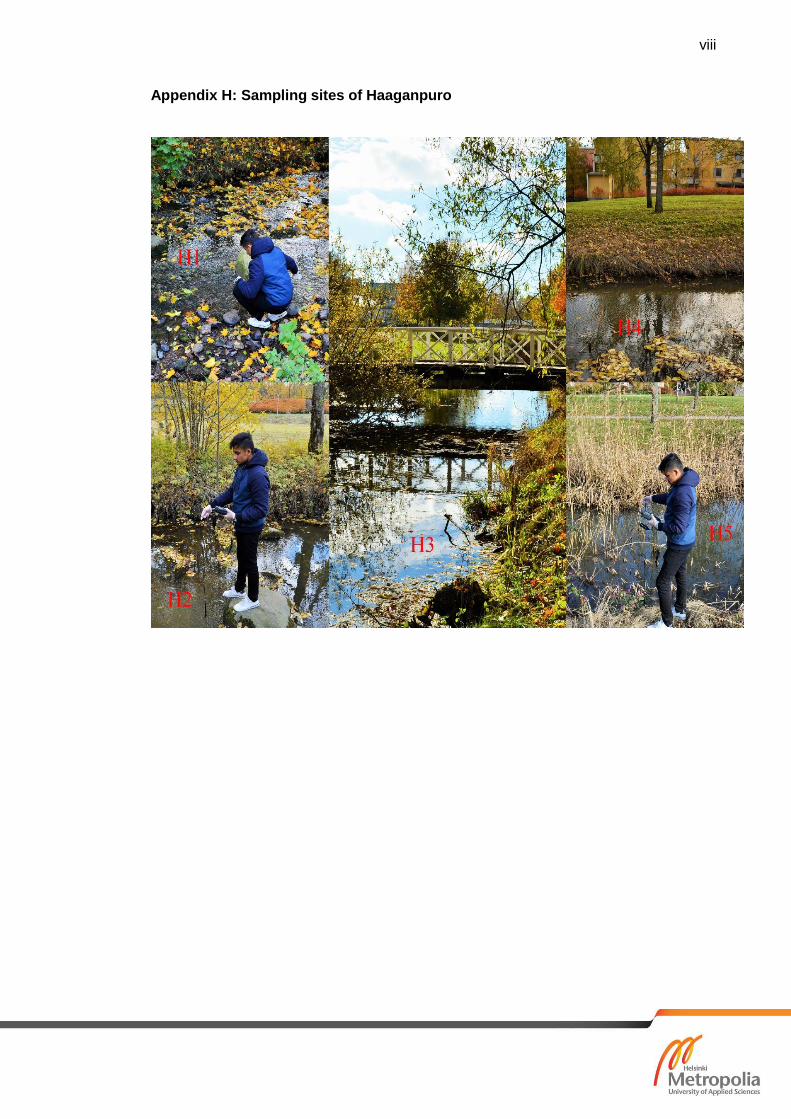
viii
Appendix H: Sampling sites of Haaganpuro
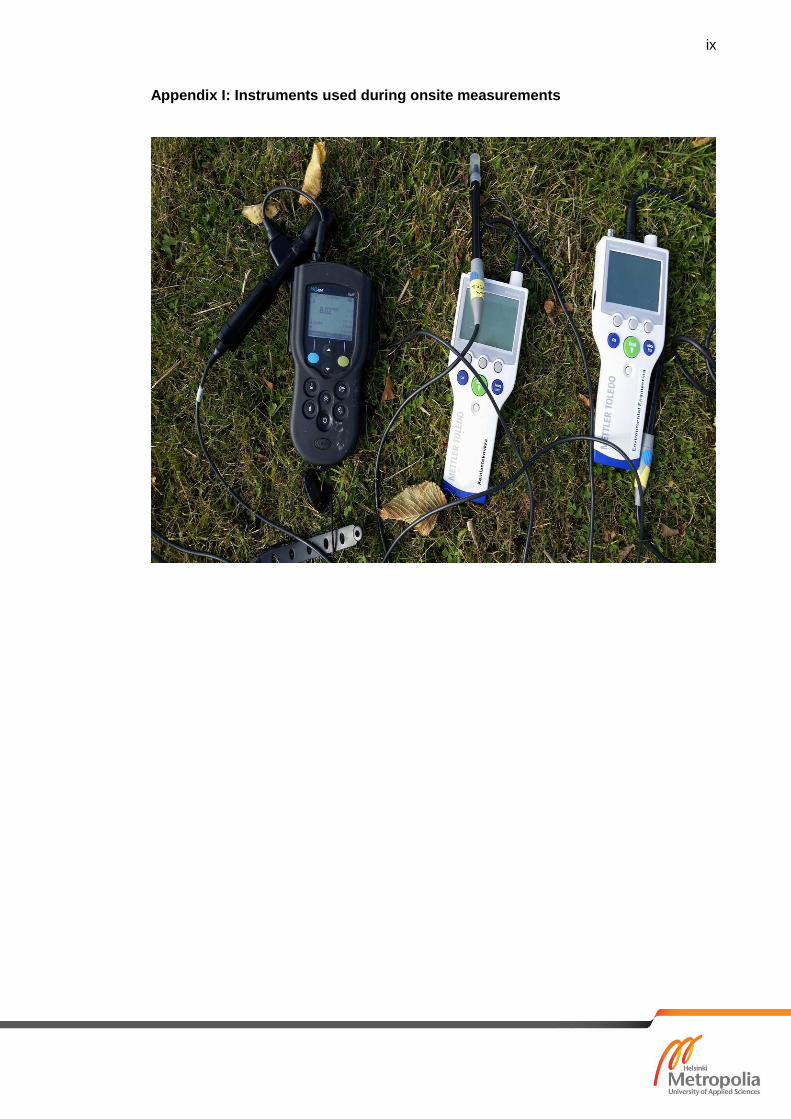
ix
Appendix I: Instruments used during onsite measurements