supplementary notes for in 2...
TRANSCRIPT

Supplementary Notes for
Corporate Financial Management
in
Southern Africa
2nd edition
by
Pieter van der Merwe (FCIS)
Version 1/2017
Chartered Secretaries Southern Africa
Riviera Office Park (Block C), 6 – 10 Riviera Road, Killarney, Johannesburg, 2193
Copyright © Chartered Secretaries Southern Africa 2015
All rights reserved. No part of this publication may be reproduced, stored in a retrieval system,
or transmitted, in any form, or by any means, electronic, mechanical, photocopying, recording
or otherwise, without prior permission, in writing, from the publisher.

Corporate Financial Management Page 2
INTRODUCTION
Please note that this is ESSENTIAL ADDITIONAL READING and is examinable.
These notes supplement Corporate Financial Management in Southern Africa, 2nd Edition.
The objective of these supplementary notes is to provide the reader with additional support
through:
- Additional examples in order to enhance the practical understanding of some concepts;
- Further explanatory notes aimed at clarifying certain theoretical principles;
- Corrections to some of the mistakes in the text;
- Revised formulae sheet incorporating updates and amendments.
The instructions have been colour coded as follows:
Add: - this means that additional information has been supplied
Replace: this means that a correction has been made
They follow the page numbers in the text book consecutively.
We hope that this supplement will enhance and clarify the related topics in the textbook.
Corporate Financial Management Page 3
1. Replace the word “SA” in the first line under heading 1.8 on page 42 with the word
“international”.
2. Add to the top of page 71:
“Consequently, ordinary shareholders expect a higher return than debenture holders do,
as debenture interest will be paid each year whatever the financial results, whereas
payment of dividends is not guaranteed.”
3. Replace the word “standing” in the second line of the first paragraph on page 72 with the
word “trading”.
4. Add at the end of the example on top of page 77 (after 8.97%):
“The realised compound yield is based on the same principal as the modified internal rate
of return (MIRR) in Part 5, Chapter 1.”
5. Replace the Growth rate (g) formula at the bottom of page 97 with the following formula:
𝑔 = √𝐿𝑎𝑡𝑒𝑠𝑡 𝑑𝑖𝑣𝑖𝑑𝑒𝑛𝑑
𝐸𝑎𝑟𝑙𝑖𝑒𝑠𝑡 𝑑𝑖𝑣𝑖𝑑𝑒𝑛𝑑
𝑛
− 1
6. At the bottom of page 106, after the question box, add the following:
Interest rate conversions
Interest rates are quoted by the banks and in the financial markets based on compounding conventions. The compounding conventions most frequently used are as follows:
- nacm nominal annual compounded monthly
- nacq nominal annual compounded quarterly
- nacs nominal annual compounded semi-annually
- naca nominal annual compounded annually (the effective rate)
In order to make accurate comparisons between interest rates, whether it is for investment or
borrowing purposes, the rates must be on the same compounding basis. Should the rates not
be on the same compounding basis, they must first be converted as such in order for them to
be comparable. Care should be taken when comparing interest rates at face value as it may
result in wrong decision making. There are a few methods by which such conversions can be
done, following is one such method or formula:
o
M
M
iio
M
MRR i
o
12x }1]))
12 x(1{[(
where: Ro = Rate of interest required (output)
Ri = Rate of interest to be converted (input) Mo = Number of months required (output) Mi = Number of months corresponding with Ri above (input)
Corporate Financial Management Page 4
PRACTICAL EXAMPLES
1. ABC Ltd has bought factory premises at prime less 1%. Given that prime is at 9.25%,
what is the effective rate of interest that the company pays per year. Answer:
Prime is an interest rate compounded monthly (nacm) while the effective rate is the annual rate (naca). Ri = 9.25% - 1.00% = 8.25% nacm Mo = 12 months Mi = 1 month
12
12x }1]))
12
1 x%25.8(1{[( 1
12
oR
naca %87.8oR
2. Green Bank is offering investors the following fixed deposit rates:
6 months: 6.50% 12 months: 6.60%
Which rate is the more attractive investment rate? Answer:
The rates cannot be compared as stated above, as they are not quoted on a comparable basis i.e. the 6 months rate is nacs and the 12-month rate is naca. The one rate must first be converted into the other rate’s compounding convention for them to be comparable. Converting the nacs rate to naca as follows: Ri = 6.50% Mo = 12 months Mi = 6 months
12
12x }1]))
12
6 x%50.6(1{[( 6
12
oR
naca %61.6oR
Thus, the 6 months rate quoted at 6.50% provides a higher annual effective rate of 6.61% compared to the 12 months quoted rate at 6.60%. Rather invest in the 6 month fixed deposit offering (though it is very marginal). To convert the 6.61% naca back to a semi-annual rate (nacs), the formula would be: Ri = 6.61% Mo = 6 months
o
M
M
iio
M
MRR i
o
12x }1]))
12 x(1{[(
o
M
M
iio
M
MRR i
o
12x }1]))
12 x(1{[(

Corporate Financial Management Page 5
Mi = 12 months
6
12x }1]))
12
12 x%61.6(1{[( 12
6
oR
nacs %50.6oR
7. Replace the formula and its workings at the bottom of page 113 with the following:
13.75
1.70) (y 0.72
10
)60.2(72.0 =
shares of no.
Interest) - t)(EBIT-(1 = EPS
y
13.75
12.24 y 7.21.8720.72y
13.75(0.72y −1.872) = 7.2y −12.24
9.90y − 25.74 = 7.2y −12.24
9.90y − 7.2y = 25.74 −12.24
2.70y = 13.50
2.70
13.50 =y
y = 5
8. Replace the Figure: Head and shoulders at the bottom of page 136 with the following figure
and commentary:
What is important with this pattern (and other patterns) is to establish the target that the share
price is expected to reach after the fall below the neckline. In this instance, the target from
where the share price breaks the neckline downwards is equal to the distance between the
5
7
9
11
13
15
17
19
21
1/J
an/1
0
1/M
ar/1
0
1/M
ay/1
0
1/J
ul/
10
1/S
ep/1
0
1/N
ov/
10
1/J
an/1
1
1/M
ar/1
1
1/M
ay/1
1
1/J
ul/
11
1/S
ep/1
1
1/N
ov/
11
1/J
an/1
2
1/M
ar/1
2
1/M
ay/1
2
1/J
ul/
12
1/S
ep/1
2
1/N
ov/
12
1/J
an/1
3
1/M
ar/1
3
1/M
ay/1
3
1/J
ul/
13
1/S
ep/1
3
1/N
ov/
13
Share Price
Left Shoulder
HeadRight Shoulder
NecklineTarget
Corporate Financial Management Page 6
neckline and the head (indicated by the two straight arrows). Note that this is not an exact
science but only a calculated estimate.
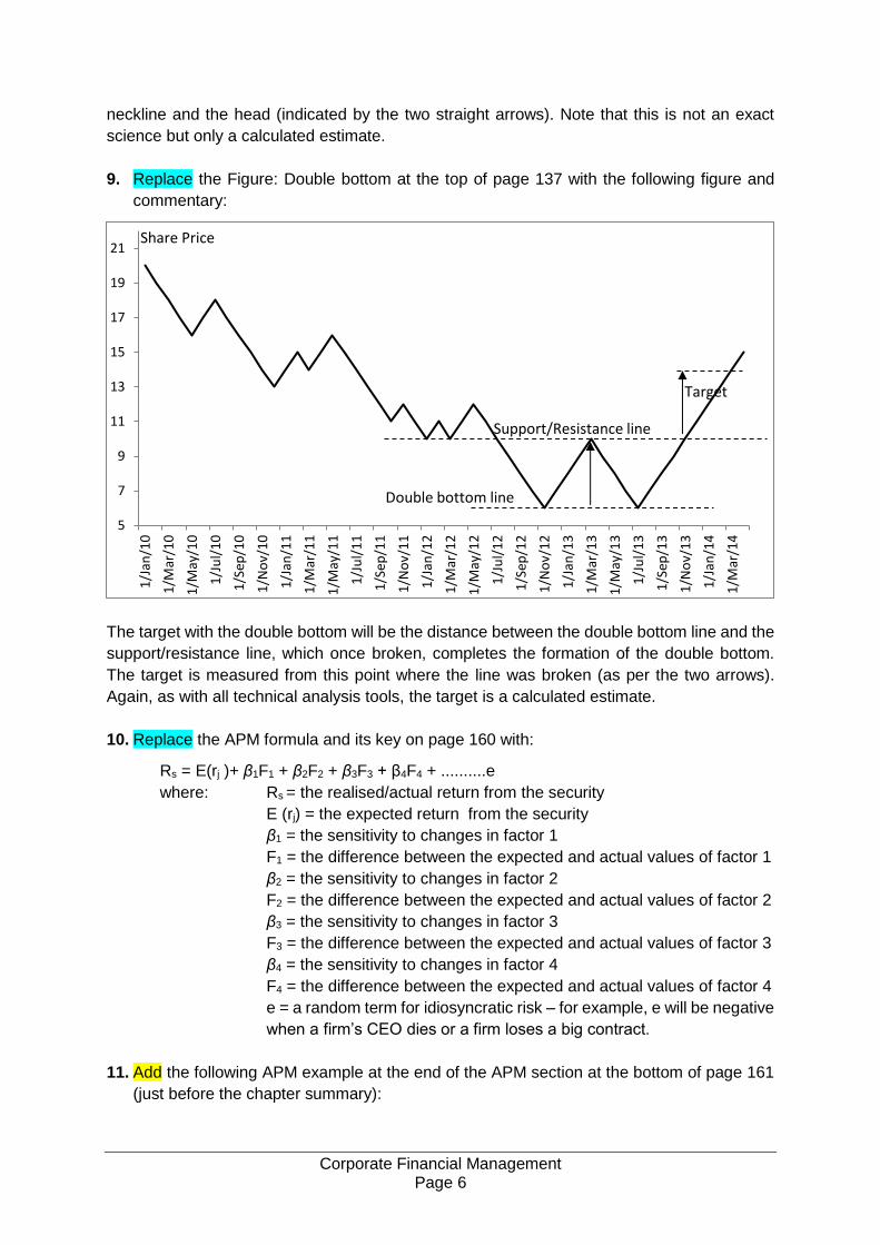
9. Replace the Figure: Double bottom at the top of page 137 with the following figure and
commentary:
The target with the double bottom will be the distance between the double bottom line and the
support/resistance line, which once broken, completes the formation of the double bottom.
The target is measured from this point where the line was broken (as per the two arrows).
Again, as with all technical analysis tools, the target is a calculated estimate.
10. Replace the APM formula and its key on page 160 with:
Rs = E(rj )+ β1F1 + β2F2 + β3F3 + β4F4 + ..........e
where: Rs = the realised/actual return from the security
E (rj) = the expected return from the security
β1 = the sensitivity to changes in factor 1
F1 = the difference between the expected and actual values of factor 1
β2 = the sensitivity to changes in factor 2
F2 = the difference between the expected and actual values of factor 2
β3 = the sensitivity to changes in factor 3
F3 = the difference between the expected and actual values of factor 3
β4 = the sensitivity to changes in factor 4
F4 = the difference between the expected and actual values of factor 4
e = a random term for idiosyncratic risk – for example, e will be negative
when a firm’s CEO dies or a firm loses a big contract.
11. Add the following APM example at the end of the APM section at the bottom of page 161
(just before the chapter summary):
5
7
9
11
13
15
17
19
21
1/J
an/1
0
1/M
ar/1
0
1/M
ay/1
0
1/J
ul/
10
1/S
ep/1
0
1/N
ov/
10
1/J
an/1
1
1/M
ar/1
1
1/M
ay/1
1
1/J
ul/
11
1/S
ep/1
1
1/N
ov/
11
1/J
an/1
2
1/M
ar/1
2
1/M
ay/1
2
1/J
ul/
12
1/S
ep/1
2
1/N
ov/
12
1/J
an/1
3
1/M
ar/1
3
1/M
ay/1
3
1/J
ul/
13
1/S
ep/1
3
1/N
ov/
13
1/J
an/1
4
1/M
ar/1
4
Share Price
Support/Resistance line
Double bottom line
Target
Corporate Financial Management Page 7
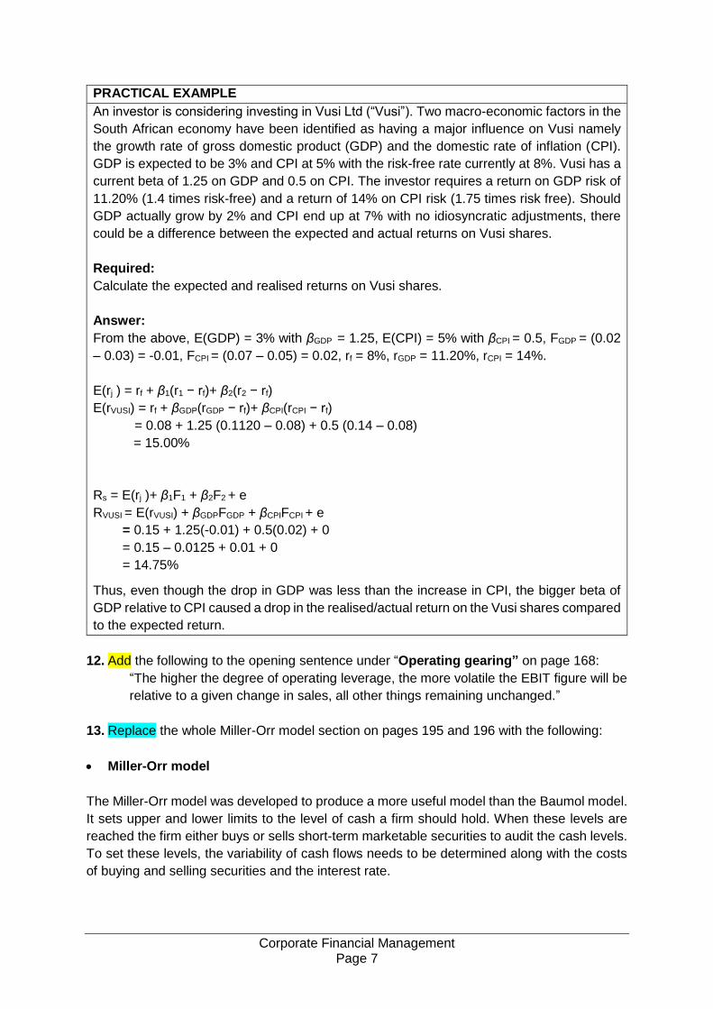
PRACTICAL EXAMPLE
An investor is considering investing in Vusi Ltd (“Vusi”). Two macro-economic factors in the
South African economy have been identified as having a major influence on Vusi namely
the growth rate of gross domestic product (GDP) and the domestic rate of inflation (CPI).
GDP is expected to be 3% and CPI at 5% with the risk-free rate currently at 8%. Vusi has a
current beta of 1.25 on GDP and 0.5 on CPI. The investor requires a return on GDP risk of
11.20% (1.4 times risk-free) and a return of 14% on CPI risk (1.75 times risk free). Should
GDP actually grow by 2% and CPI end up at 7% with no idiosyncratic adjustments, there
could be a difference between the expected and actual returns on Vusi shares.
Required:
Calculate the expected and realised returns on Vusi shares.
Answer:
From the above, E(GDP) = 3% with βGDP = 1.25, E(CPI) = 5% with βCPI = 0.5, FGDP = (0.02
– 0.03) = -0.01, FCPI = (0.07 – 0.05) = 0.02, rf = 8%, rGDP = 11.20%, rCPI = 14%.
E(rj ) = rf + β1(r1 − rf)+ β2(r2 − rf)
E(rVUSI) = rf + βGDP(rGDP − rf)+ βCPI(rCPI − rf)
= 0.08 + 1.25 (0.1120 – 0.08) + 0.5 (0.14 – 0.08)
= 15.00%
Rs = E(rj )+ β1F1 + β2F2 + e
RVUSI = E(rVUSI) + βGDPFGDP + βCPIFCPI + e
= 0.15 + 1.25(-0.01) + 0.5(0.02) + 0
= 0.15 – 0.0125 + 0.01 + 0
= 14.75%
Thus, even though the drop in GDP was less than the increase in CPI, the bigger beta of
GDP relative to CPI caused a drop in the realised/actual return on the Vusi shares compared
to the expected return.
12. Add the following to the opening sentence under “Operating gearing” on page 168:
“The higher the degree of operating leverage, the more volatile the EBIT figure will be
relative to a given change in sales, all other things remaining unchanged.”
13. Replace the whole Miller-Orr model section on pages 195 and 196 with the following:
• Miller-Orr model
The Miller-Orr model was developed to produce a more useful model than the Baumol model.
It sets upper and lower limits to the level of cash a firm should hold. When these levels are
reached the firm either buys or sells short-term marketable securities to audit the cash levels.
To set these levels, the variability of cash flows needs to be determined along with the costs
of buying and selling securities and the interest rate.
Corporate Financial Management Page 8
The steps in using the model are:
• Determine the lower level of cash the firm is happy to have. This is generally set at a
minimum safety level, which in theory could be zero.
• Determine the variance of the firm’s cash flows (perhaps over a three or six month period).
• Calculate the spread between the minimum (lower) and maximum (upper) cash balance
limits, using the following formula:
Spread=3×√0.75 × variance of cash flow × transaction cost
interest rate
3
• Calculate the upper limit – this is the lower limit plus the spread.
• However, to minimise the cost of holding excess cash and to avoid the danger of
insufficient cash, a pre-calculated target level of cash holdings (the return point) is
determined. The return point is the lower limit plus ⅓ of the spread.
PRACTICAL EXAMPLE
Pull Ltd faces an interest rate of 0.5% per day and its brokers charge R75 for each
transaction in short-term securities. The managing director of Pull Ltd has stated that the
minimum cash balance that is acceptable is R2 000 and that the variance of cash flows on
a daily basis is R16 000 (standard deviation of daily cash flows is thus R126.49 (rounded)).
Required:
What is the maximum level of cash the firm should hold and at what point should it start to
purchase or sell securities?
Following the above procedure:
• Determine the lower level of cash the firm is happy to have – this has been set at R2 000.
• Determine the variation in cash flows of the firm – this has been found to be R16 000.
• Calculate the spread of transactions.
• Calculate the upper limit.
Answer:
Spread=3×√(0.75×16000×75)
0.005
3
= R1 694
• Calculate the upper limit – this is the sum of the lower limit and the spread:
Upper limit = R2 000 + R1 694 = R3 694
• Securities should be sold when the lower level is reached. The amount of securities to
be sold is equal to the difference between the lower level and the return point. The return
point is the sum of the lower limit and ⅓ of the spread: return point = R2 000 + ⅓ (R1
694) = R2 565

Corporate Financial Management Page 9
Thus the firm is aiming for a cash holding of R2 565 (the return point). Therefore, if the
balance of cash reaches R3 694 the firm should buy R3 694 - R2 565 = R1 129 of
marketable securities and if it falls to R2 000 then R565 of securities should be sold.
The Miller-Orr model is useful in that it considers:
• the level of interest rates (higher rates give a narrower spread, so less cash needs to be
held before the return point and the upper limit is reached);
• transaction costs (higher transaction costs increase the spread and therefore reduce the
number of transactions);
• variability of cash flows (more variable cash flows means more unpredictability, requiring
a higher spread to absorb the variability).
A drawback of the model is that it assumes that cash flows vary randomly and does not take
account of the fact that some cash flows (for example, dividend payments) can be predicted
accurately.
14. Replace the EOQ formula on page 217 with:
EOQ=√2 (Cost per order)(Annual usage in units)
Annual holding cost per unit
15. Add the following after the “Conclusion” in the first example on page 225:
Note: The reduction in working capital above can be broken down further. Total sales are
made up of 80% cost of sales (COS) and 20% gross profit (GP). The logic goes that the
only item that is actually been financed is the COS that had to be incurred to generate the
sales. The GP does not need to be financed but is rather caught up in the debtors figure
representing an amount that could have been banked on day one of the sale (if it was a
cash sale) and could have earned interest i.e. the interest not earned on the GP is an
opportunity cost.
Present: 2 month’s COS = 2/12 x R1.2mil x 80% = R160 000
2 month’s GP = 2/12 x R1.2mil x 20% = R40 000
New: ½ month’s COS = 30% x 0.5/12 x 0.85 x R1.2mil x 80% = R10 200
½ month’s GP = 30% x 0.5/12 x 0.85 x R1.2mil x 20% = R2 550
1 month’s COS = 70% x 1/12 x 0.85 x R1.2mil x 80% = R47 600
1 month’s GP = 70% x 1/12 x 0.85 x R1.2mil x 20% = R11 900
Working capital tied up in COS have dropped from R160 000 to R57 800 (R10 200 +
R47 600) = R102 200 at an annual saving in financing cost of R16 352.
Gross Profit tied up in working capital dropped from R40 000 to R14 450 (R2 550 +
R11 900) = R25 550 on which interest can now be earned of R4 088.
Thus, the total annual finance cost saving is R20 440 (R16 352 + R4 088).
Add the following at the end of the example on page 227:
Corporate Financial Management Page 10
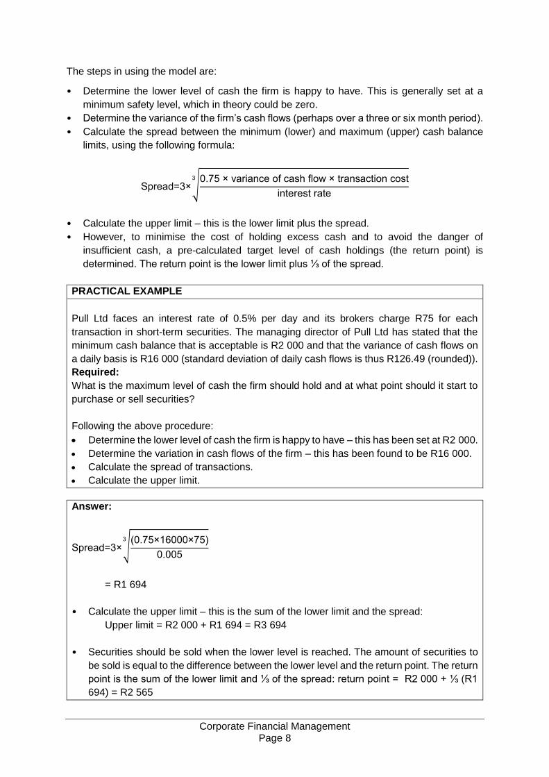
As with the example on pg.225, the reduction in working capital above can be broken down
further. Total sales are made up of 95% cost of sales (COS) and 5% gross profit (GP).
Present: 1 month’s COS = 1/12 x R1.25mil x 95% = R98 958
1 month’s GP = 1/12 x R1.25mil x 5% = R5 208
New: 2 month’s COS = 2/12 x R1.75mil x 95% = R277 083
Increased Working Capital (ex. Debtors) = R50 000
2 month’s GP = 2/12 x R1.75mil x 5% = R14 583
Working capital tied up in COS have increased from R98 958 to R327 083 (R277 083 +
R50 000) = R228 125 at an annual increase in financing cost of R34 219.
Gross Profit tied up in working capital increased from R5 208 to R14 583 = R9 375 on which
interest could have been earned of R1 406.
Thus, the total annual increase in financing cost is R35 625 (R34 219 + R1 406).
16. Replace: The second sentence after the practical example time line on page 243 should
read:
“However the last seven do represent such an annuity.” (not last six as per the text)
17. Remove the third sentence of the first paragraph under the heading “The second way of
calculating” on page 246 i.e. remove the wording:
“See Guidance Note 2: Annuities”. (There are no more guidance notes)
18. Replace the formula on page 249 and page 253 with the following formula:
IRR = low rate +
rate) low - ratehigh (
rate)high NPV - rate low (NPV
rate low NPV
19. Replace the whole of paragraphs 1.7.1 and 1.7.2 from pages 253 to 255 with the following:
1.7.1 Multiple solutions: a possible further drawback of IRR
Most capital investment projects involve an initial investment – with cash outflows – followed
by a series of cash inflows in later years. This is called a conventional cash flow pattern.
Sometimes the cash flows change direction again in later years.
Typically, this happens when there are closure costs that cause cash outflows at the end of
the project. An example of this could be a nuclear power station, where decommissioning
costs at the end of the station’s life are very high. Another example could be a chemical
production facility, where decontamination has to be done when the facility is closed down, at
a cash cost greater than any operating cash inflow in the final year. If the cash flows change
direction more than once, the cash flows are said to be ‘non-conventional’. With non-
conventional cash flows, the internal rate of return can take more than one value. The following
example shows what can happen:
PRACTICAL EXAMPLE

Corporate Financial Management Page 11
Enzo Ltd is considering investing in a project i.e. Project C: the project will last for two years
and has the following details:
Cash flow Cash flow Cash flow IRR
Yr. 0 Yr. 1 Yr. 2
Project C (R907 325) R8m (R8m) 15% and
667%*
*The exact percentages are 14.999% and 666.71% (used in the table below)
Using the IRR, Project C end up with two IRR’s as the cash flows change direction at least
twice. This also assumes that that the cash flows are reinvested at the particular IRR being
used. The present values (PV’s) of the cash flows will be as follows:
Yr. 0 Yr. 1 Yr. 2 NPV
Cash Flows (R907 325) R8m (R8m)
PV’s @ 15%* (R907 325) R 6 956 586 (R6 049 261) 0
PV’s @ 667%* (R907 325) R 1 043 414 (R136 089) 0
Thus, both IRR’s provide a zero NPV result.
The net present value is zero with a discount rate of about 15% and also with a discount rate
of 667%. Between 15% and 667%, the NPV is positive. Below 15%, or above 667%, the NPV
is negative. What does this mean? Not much to practical people. A slightly different approach
is required.
1.7.2 Modified IRR (MIRR)
The problem with using the IRR is that it assumes that all cash flows from a project are
reinvested at the IRR of that particular project. By changing this assumption and applying a
more realistic reinvestment rate e.g. a money market deposit rate, this problem with IRR is
solved. The IRR arrived at by using this alternative reinvestment rate is referred to as the
modified IRR (MIRR). The same principle is applied in calculating the “realised compound
yield” of a bond in Part 2, Chapter 3.
PRACTICAL EXAMPLE
Using the same data as in the Enzo Ltd example above.
The cash flows from the project are deposited into Enzo’s money market account, earning
interest at a rate of 13.00% p.a. Thus, we need to calculate the MIRR of the project,
reinvesting the cash flows at 13.00%.
This is done by taking each cash in-flow and reinvesting it until the end of the project (end
of year 2) at 13.00% p.a. (see the table below). By adding these respective reinvested cash
flows for each project, we arrive at the Terminal Value (Future Value) of these reinvested
cash flows as at the end of the project. There are then only two cash flows used in
calculating the MIRR namely the initial investment and the accumulated Terminal Value.
Corporate Financial Management Page 12
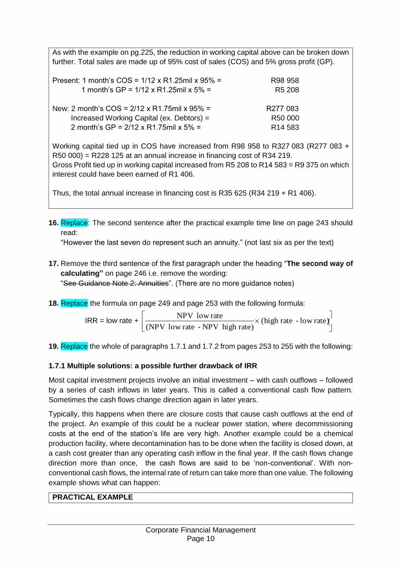
The MIRR can then be found by trial and error (as with the IRR) i.e. the rate of interest that
will make the NPV of the two cash flows equal to zero (last column in the table below).
PROJECT C:
Year Cash Flows
Years to end
of Project
FV Factor
at 13.00%
Terminal
Value
Cash Flows
and MIRR
0 (R907 325) (R907 325)
1 R8 000 000 1 1.1300 R9 040 000
2 (R8 000 000) 0 1.0000 (R8 000 000) R1 040 000*
MIRR = 7.06%
*R1 040 000 is the sum total of the individual Terminal Values from the second last column.
Thus the real IRR (MIRR) of this project is 7.06%, which is significantly lower than the 15%
and 667% IRR’s arrived at earlier.
If a company embarks on numerous projects, this then translates into multiple but different
reinvestment rates of the respective cash flows from each project. This is not a valid
assumption as all cash flows from the different projects are most probably deposited into a
single bank account or money market account, earning the same rate of interest. This rate of
interest will most probably be different to the IRRs of the respective projects. The MIRR solves
this problem by calculating each project’s IRR by reinvesting all cash flows, regardless from
which project, at the same rate of interest i.e. the rate earned on the money market account.
PRACTICAL EXAMPLE
Benso Ltd is investing in two projects i.e. Project A and Project B; both projects last three
years and have the following details:
Cash flow Cash flow Cash flow Cash flow IRR
Yr. 0 Yr. 1 Yr. 2 Yr. 3
Project A (R100 000) R15 000 R15 000 R115 000 15.00%
Project B (R100 000) R90 000 R20 000 R15 000 17.79%
Using the IRR, Project B is doing better than Project A. This assumes of course that the
cash flows from each project are reinvested at the IRR of that particular project. All cash
flows from both projects are however deposited into the Benso’s money market account,
earning interest at a rate of 11.00% p.a. Thus, we need to calculate the MIRR of each
project, reinvesting the cash flows of each project at 11.00%.
This is done by taking each cash in-flow and reinvesting it until the end of the project (end
of year 3) at 11.00% p.a. (see the table below). By adding these respective reinvested cash
flows for each project, we arrive at the Terminal Value (Future Value) of these reinvested
cash flows as at the end of each project. There are only two cash flows used in calculating
the MIRR namely the initial investment and the accumulated Terminal Value. The MIRR can
then be found by trial and error (as with the IRR) i.e. the rate of interest that will make the
NPV of the two cash flows equal to zero (last column in the tables below).
PROJECT A:
Corporate Financial Management Page 13
Year Cash Flows
and IRR
Years to end
of Project
FV Factor
at 11.00%
Terminal
Value
Cash Flows
and MIRR
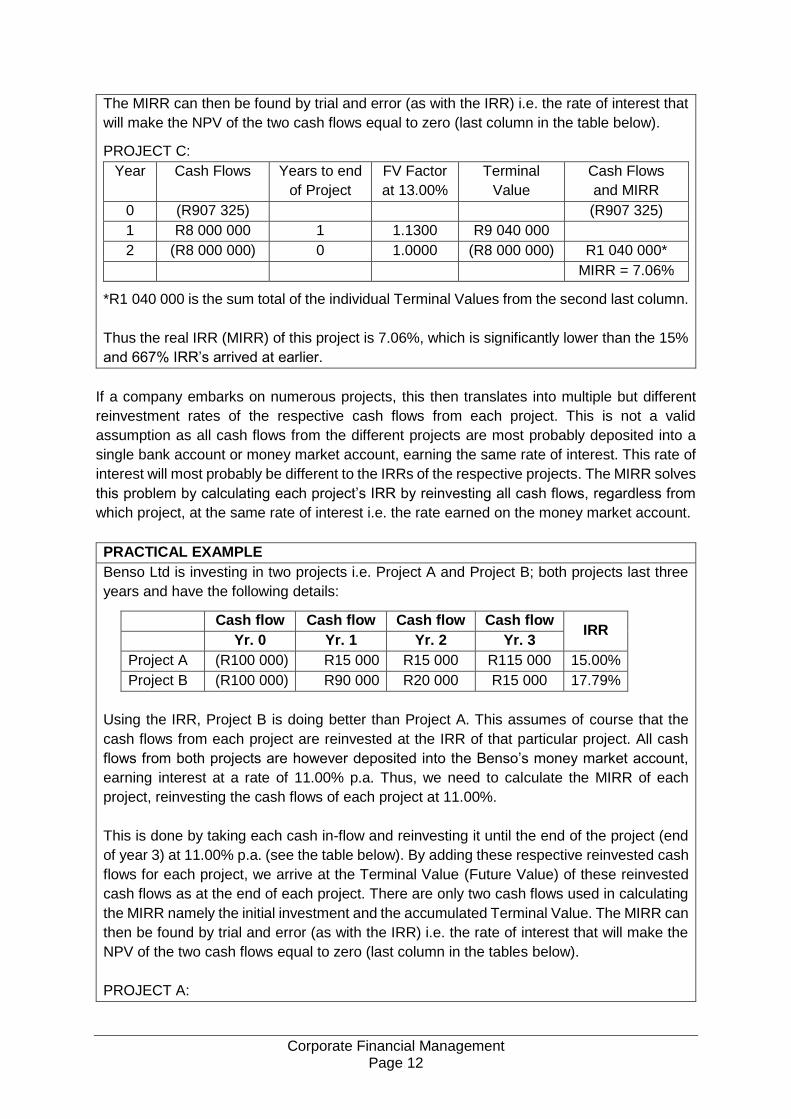
0 -R100 000 -R100 000.00
1 R15 000 2 1.2321 R18 481.50
2 R15 000 1 1.1100 R16 650.00
3 R115 000 0 1.0000 R115 000.00 R150 131.50*
IRR = 15.00% MIRR = 14.50%
*R150 131.50 is the sum total of the individual Terminal Values from the second last column.
PROJECT B:
Year Cash Flows
and IRR
Years to end
of Project
FV Factor
at 11.00%
Terminal
Value
Cash Flows
and MIRR
0 -R100 000 -R100 000.00
1 R90 000 2 1.2321 R110 889.00
2 R20 000 1 1.1100 R22 200.00
3 R15 000 0 1.0000 R15 000.00 R148 089.00*
IRR = 17.79% MIRR = 13.98%
*R148 089.00 is the sum total of the individual Terminal Values from the second last column.
Based on the MIRR, Project A at 14.50% is now more lucrative than Project B at 13.98%
(opposite to the IRR result). This illustrates the importance of the effect that the reinvestment
rate has on the projects above and on investments in general. The reinvestment rate used
determines the degree and power of the compounding effect. Instead of using the money
market deposit rate as in this example, companies can also use their cost of capital as the
reinvestment rate for the cash flows from their various projects.
20. Replace the wording as indicated below in the second sentence of the first paragraph
under “Earnings per share” on page 287:
“An example is given is section 8 below”. (there is no section 8)
21. Replace the whole of paragraph 1.5 from pages 293 to 296 with the following:
1.5 SYNERGIES
The object of a merger may be to obtain operating benefits that exceed the scope of operations
of the individual companies involved in the merger. The “excess benefit” is often referred to
as the benefit of synergies. Note that these benefits can be expressed either as a single value
(representing “P” in the P/E formula) or as annual synergy earnings (representing “E” in the
P/E formula), which can be converted into “P” by multiplying “E” with the P/E ratio.
These benefits may be dealt with as follows:
• The benefit may be apportioned pro-rata between the acquiring company and the target
company.
• The benefit may be allocated entirely to the target company’s shareholders in arriving at
the share offer price.
Corporate Financial Management Page 14
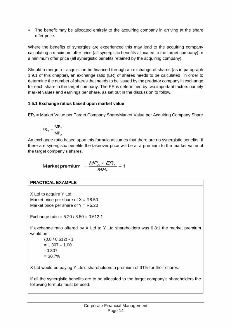
• The benefit may be allocated entirely to the acquiring company in arriving at the share
offer price.
Where the benefits of synergies are experienced this may lead to the acquiring company
calculating a maximum offer price (all synergistic benefits allocated to the target company) or
a minimum offer price (all synergistic benefits retained by the acquiring company).
Should a merger or acquisition be financed through an exchange of shares (as in paragraph
1.9.1 of this chapter), an exchange ratio (ER) of shares needs to be calculated in order to
determine the number of shares that needs to be issued by the predator company in exchange
for each share in the target company. The ER is determined by two important factors namely
market values and earnings per share, as set out in the discussion to follow.
1.5.1 Exchange ratios based upon market value
ERT = Market Value per Target Company Share/Market Value per Acquiring Company Share
A
TT
MP
MPER
An exchange ratio based upon this formula assumes that there are no synergistic benefits. If
there are synergistic benefits the takeover price will be at a premium to the market value of
the target company’s shares.
1premium Market
T
TA
MP
ER MP
PRACTICAL EXAMPLE
X Ltd to acquire Y Ltd.
Market price per share of X = R8.50
Market price per share of Y = R5.20
Exchange ratio = 5.20 / 8.50 = 0.612:1
If exchange ratio offered by X Ltd to Y Ltd shareholders was 0.8:1 the market premium
would be:
(0.8 / 0.612) - 1
= 1.307 – 1.00
=0.307
= 30.7%
X Ltd would be paying Y Ltd’s shareholders a premium of 31% for their shares.
If all the synergistic benefits are to be allocated to the target company’s shareholders the
following formula must be used:
Corporate Financial Management Page 15
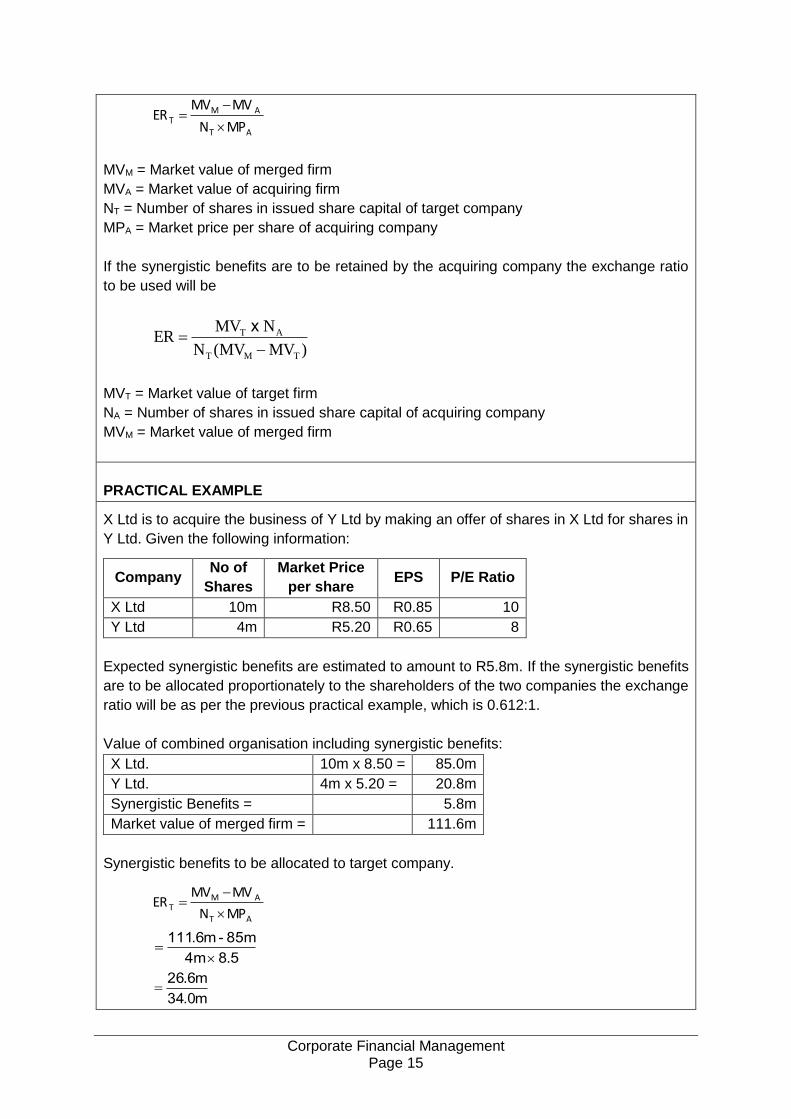
AT
AMT
MP N
MVMVER
MVM = Market value of merged firm
MVA = Market value of acquiring firm
NT = Number of shares in issued share capital of target company
MPA = Market price per share of acquiring company
If the synergistic benefits are to be retained by the acquiring company the exchange ratio
to be used will be
)MV (MVN
N MVER
TMT
AT
x
MVT = Market value of target firm
NA = Number of shares in issued share capital of acquiring company
MVM = Market value of merged firm
PRACTICAL EXAMPLE
X Ltd is to acquire the business of Y Ltd by making an offer of shares in X Ltd for shares in
Y Ltd. Given the following information:
Company No of
Shares
Market Price
per share EPS P/E Ratio
X Ltd 10m R8.50 R0.85 10
Y Ltd 4m R5.20 R0.65 8
Expected synergistic benefits are estimated to amount to R5.8m. If the synergistic benefits
are to be allocated proportionately to the shareholders of the two companies the exchange
ratio will be as per the previous practical example, which is 0.612:1.
Value of combined organisation including synergistic benefits:
X Ltd. 10m x 8.50 = 85.0m
Y Ltd. 4m x 5.20 = 20.8m
Synergistic Benefits = 5.8m
Market value of merged firm = 111.6m
Synergistic benefits to be allocated to target company.
584m
85m-m6111
.
.
m034
m626
.
.
AT
AMT
MP N
MVMVER
Corporate Financial Management Page 16
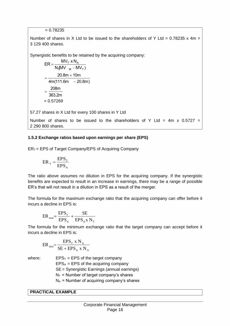
= 0.78235
Number of shares in X Ltd to be issued to the shareholders of Y Ltd = 0.78235 x 4m =
3 129 400 shares.
Synergistic benefits to be retained by the acquiring company:
)TMT
AT
MV (MVN
N x MVER
)20.8m 4m(111.6m
10m20.8m
363.2m
208m
= 0.57269
57.27 shares in X Ltd for every 100 shares in Y Ltd
Number of shares to be issued to the shareholders of Y Ltd = 4m x 0.5727 =
2 290 800 shares.
1.5.2 Exchange ratios based upon earnings per share (EPS)
ERT = EPS of Target Company/EPS of Acquiring Company
A
T
TEPS
EPSER
The ratio above assumes no dilution in EPS for the acquiring company. If the synergistic
benefits are expected to result in an increase in earnings, there may be a range of possible
ER’s that will not result in a dilution in EPS as a result of the merger.
The formula for the maximum exchange ratio that the acquiring company can offer before it
incurs a decline in EPS is:
TAA
Tmax
Nx EPS
SE
EPS
EPSER
The formula for the minimum exchange ratio that the target company can accept before it
incurs a decline in EPS is:
AA
AT
minN x EPS SE
N x EPSER
where: EPST = EPS of the target company
EPSA = EPS of the acquiring company
SE = Synergistic Earnings (annual earnings)
NT = Number of target company’s shares
NA = Number of acquiring company’s shares
PRACTICAL EXAMPLE
Corporate Financial Management Page 17
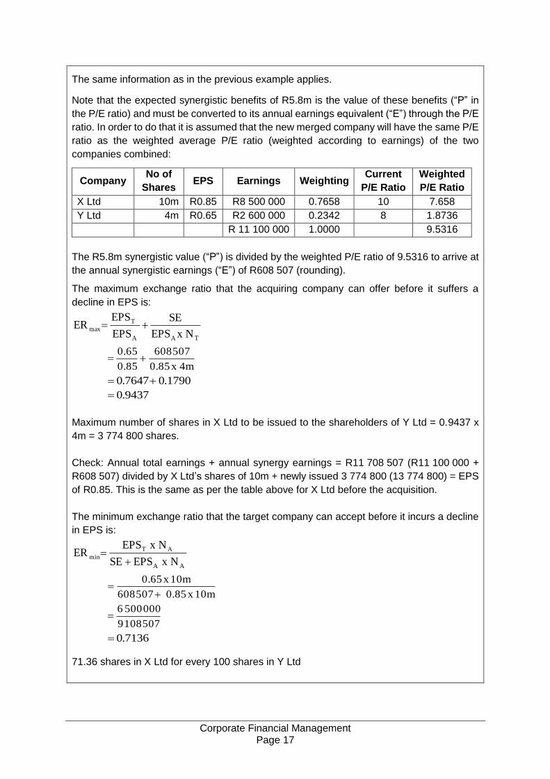
The same information as in the previous example applies.
Note that the expected synergistic benefits of R5.8m is the value of these benefits (“P” in
the P/E ratio) and must be converted to its annual earnings equivalent (“E”) through the P/E
ratio. In order to do that it is assumed that the new merged company will have the same P/E
ratio as the weighted average P/E ratio (weighted according to earnings) of the two
companies combined:
Company No of
Shares EPS Earnings Weighting
Current
P/E Ratio
Weighted
P/E Ratio
X Ltd 10m R0.85 R8 500 000 0.7658 10 7.658
Y Ltd 4m R0.65 R2 600 000 0.2342 8 1.8736
R 11 100 000 1.0000 9.5316
The R5.8m synergistic value (“P”) is divided by the weighted P/E ratio of 9.5316 to arrive at
the annual synergistic earnings (“E”) of R608 507 (rounding).
The maximum exchange ratio that the acquiring company can offer before it suffers a
decline in EPS is:
TAA
T
maxNx EPS
SE
EPS
EPSER
4m x 0.85
507 608
0.85
0.65
1790.07647.0
9437.0
Maximum number of shares in X Ltd to be issued to the shareholders of Y Ltd = 0.9437 x
4m = 3 774 800 shares.
Check: Annual total earnings + annual synergy earnings = R11 708 507 (R11 100 000 +
R608 507) divided by X Ltd’s shares of 10m + newly issued 3 774 800 (13 774 800) = EPS
of R0.85. This is the same as per the table above for X Ltd before the acquisition.
The minimum exchange ratio that the target company can accept before it incurs a decline
in EPS is:
AA
AT
minN x EPS SE
N x EPSER
10m x 0.85 507 608
10m x 0.65
507 108 9
000 500 6
7136.0
71.36 shares in X Ltd for every 100 shares in Y Ltd
Corporate Financial Management Page 18
Number of shares to be issued to the shareholders of Y Ltd = 4m x 0.7136 = 2 854
400 shares.
Check: Annual total earnings + annual synergy earnings = R11 708 507 (R11 100 000 +
R608 507). Y Ltd shareholder’s proportion of this income will be 2 854 400/(2 854 400 +
10m) = 22.21% x R11 708 507 = R2 599 947. The EPS will then be R2 599 947 divided by
Y Ltd’s original share issue of 4m = R0.65 per share. This is the same as per the table
above for Y Ltd before the acquisition.
Should the decision be to base the acquisition on market value, there might still be a
requirement to prevent a dilution in EPS. The acquiring company might then structure an offer
through convertible debentures with conversion to ordinary shares at a later stage, when
earnings are of an adequate size so that the EPS after conversion is the same as at the time
of the merger. Another alternative is the issue of convertible preferred ordinary shares with a
fixed preferred ordinary dividend. These shares will be convertible into ordinary shares when
the ordinary dividend reaches a level that will equate to the fixed preferred ordinary dividend.
This should coincide with an EPS that is the same as at the time of the merger.
22. Replace the sentence in the “Answer:” section at the bottom of page 303 that reads
“Shares in Modali received = 10m x 2 = R10m shares” with “Shares in Modali received =
10m x 2 = 20m shares”
23. Replace the whole of paragraph 1.7 from pages 345 to 346 with the following:
1.7 BUYING AND SELLING FOREIGN CURRENCY
Many firms and individuals buy any foreign currency they need from their bank and sell the
bank any foreign currency they want converted into Rands. In these transactions the bank is
selling and then buying, the currency respectively. The rates that banks charge are quoted
typically as such (exchange rates are also shown in a similar fashion in the financial press):
Value of the Rand against other currencies (spot rates)
US Dollar 11.3700 - 11.7200
Euro 13.1812 - 13.6784
Pound Sterling 17.2233 - 17.8261
(Note that these rates vary on a daily basis and the figures given here are for illustration only.)
• In the quotations above, the US Dollar, Euro and Pound Sterling are referred to as the
base currencies while the Rand is the variable currency.
• A spot rate is the rate used for immediate transactions and quotations for which no
previous arrangements have been made. Delivery to the buyer is made two days later.
• A forward rate is the rate quoted for a transaction at a defined date in the future, e.g. one
month forward and three months forward being for one month and three months in the
future respectively.
The first point to note is that there is a spread in each rate. This represents the dealer’s (the
bank’s) turn or profit. So company A selling US dollars to the bank would receive a smaller
amount in Rand than company B would have to pay the bank to buy the same amount of
Corporate Financial Management Page 19
US dollars from the bank. For example, if a SA exporter has sold goods for $1 million, he will
probably sell the US$ to the bank and will receive R11 370 000 from which the bank will
generally deduct commission. An SA importer buying $1 million from the bank will pay R11 720
000, plus the bank’s commission.
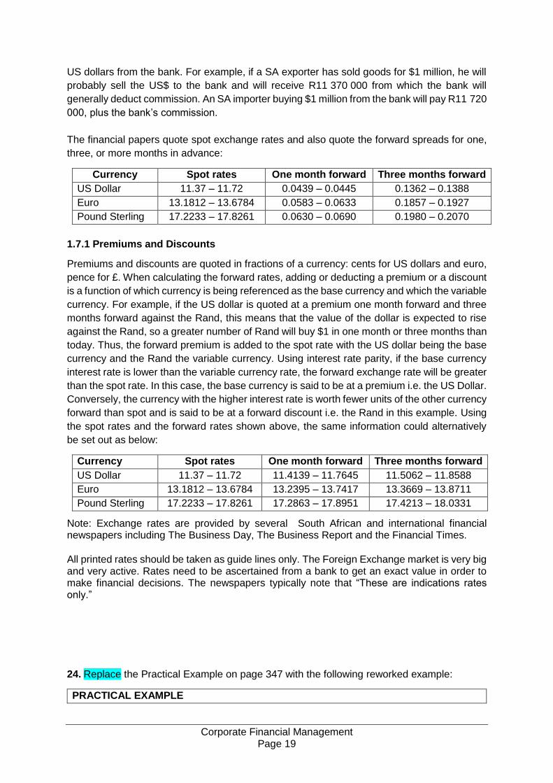
The financial papers quote spot exchange rates and also quote the forward spreads for one,
three, or more months in advance:
Currency Spot rates One month forward Three months forward
US Dollar 11.37 – 11.72 0.0439 – 0.0445 0.1362 – 0.1388
Euro 13.1812 – 13.6784 0.0583 – 0.0633 0.1857 – 0.1927
Pound Sterling 17.2233 – 17.8261 0.0630 – 0.0690 0.1980 – 0.2070
1.7.1 Premiums and Discounts
Premiums and discounts are quoted in fractions of a currency: cents for US dollars and euro,
pence for £. When calculating the forward rates, adding or deducting a premium or a discount
is a function of which currency is being referenced as the base currency and which the variable
currency. For example, if the US dollar is quoted at a premium one month forward and three
months forward against the Rand, this means that the value of the dollar is expected to rise
against the Rand, so a greater number of Rand will buy $1 in one month or three months than
today. Thus, the forward premium is added to the spot rate with the US dollar being the base
currency and the Rand the variable currency. Using interest rate parity, if the base currency
interest rate is lower than the variable currency rate, the forward exchange rate will be greater
than the spot rate. In this case, the base currency is said to be at a premium i.e. the US Dollar.
Conversely, the currency with the higher interest rate is worth fewer units of the other currency
forward than spot and is said to be at a forward discount i.e. the Rand in this example. Using
the spot rates and the forward rates shown above, the same information could alternatively
be set out as below:
Currency Spot rates One month forward Three months forward
US Dollar 11.37 – 11.72 11.4139 – 11.7645 11.5062 – 11.8588
Euro 13.1812 – 13.6784 13.2395 – 13.7417 13.3669 – 13.8711
Pound Sterling 17.2233 – 17.8261 17.2863 – 17.8951 17.4213 – 18.0331
Note: Exchange rates are provided by several South African and international financial newspapers including The Business Day, The Business Report and the Financial Times.
All printed rates should be taken as guide lines only. The Foreign Exchange market is very big and very active. Rates need to be ascertained from a bank to get an exact value in order to make financial decisions. The newspapers typically note that “These are indications rates only.”
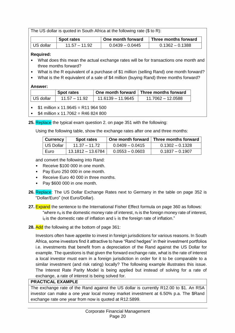
24. Replace the Practical Example on page 347 with the following reworked example:
PRACTICAL EXAMPLE
Corporate Financial Management Page 20
The US dollar is quoted in South Africa at the following rate ($ to R):
Spot rates One month forward Three months forward
US dollar 11.57 – 11.92 0.0439 – 0.0445 0.1362 – 0.1388
Required:
• What does this mean the actual exchange rates will be for transactions one month and
three months forward?
• What is the R equivalent of a purchase of $1 million (selling Rand) one month forward?
• What is the R equivalent of a sale of $4 million (buying Rand) three months forward?
Answer:
Spot rates One month forward Three months forward
US dollar 11.57 – 11.92 11.6139 – 11.9645 11.7062 – 12.0588
• $1 million x 11.9645 = R11 964 500
• $4 million x 11.7062 = R46 824 800
25. Replace the typical exam question 2. on page 351 with the following:
Using the following table, show the exchange rates after one and three months:
Currency Spot rates One month forward Three months forward
US Dollar 11.37 – 11.72 0.0409 – 0.0415 0.1302 – 0.1328
Euro 13.1812 – 13.6784 0.0553 – 0.0603 0.1837 – 0.1907
and convert the following into Rand:
• Receive $100 000 in one month.
• Pay Euro 250 000 in one month.
• Receive Euro 40 000 in three months.
• Pay $600 000 in one month.
26. Replace: The US Dollar Exchange Rates next to Germany in the table on page 352 is
“Dollar/Euro” (not Euro/Dollar).
27. Expand the sentence to the International Fisher Effect formula on page 360 as follows:
“where nd is the domestic money rate of interest, nf is the foreign money rate of interest,
id is the domestic rate of inflation and if is the foreign rate of inflation.”
28. Add the following at the bottom of page 361:
Investors often have appetite to invest in foreign jurisdictions for various reasons. In South
Africa, some investors find it attractive to have “Rand hedges” in their investment portfolios
i.e. investments that benefit from a depreciation of the Rand against the US Dollar for
example. The questions is that given the forward exchange rate, what is the rate of interest
a local investor must earn in a foreign jurisdiction in order for it to be comparable to a
similar investment (and risk rating) locally? The following example illustrates this issue.
The Interest Rate Parity Model is being applied but instead of solving for a rate of
exchange, a rate of interest is being solved for.
PRACTICAL EXAMPLE
The exchange rate of the Rand against the US dollar is currently R12.00 to $1. An RSA
investor can make a one year local money market investment at 6.50% p.a. The $Rand
exchange rate one year from now is quoted at R12.5899.
Corporate Financial Management Page 21
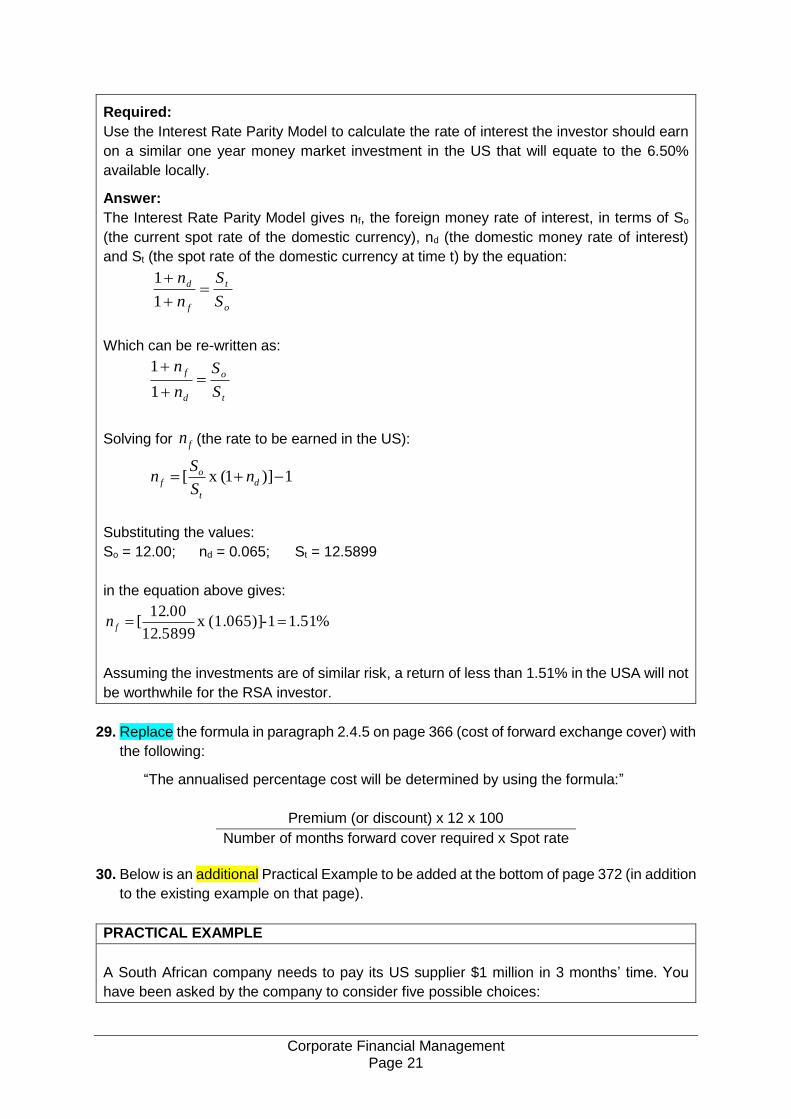
Required:
Use the Interest Rate Parity Model to calculate the rate of interest the investor should earn
on a similar one year money market investment in the US that will equate to the 6.50%
available locally.
Answer:
The Interest Rate Parity Model gives nf, the foreign money rate of interest, in terms of So
(the current spot rate of the domestic currency), nd (the domestic money rate of interest)
and St (the spot rate of the domestic currency at time t) by the equation:
o
t
f
d
S
S
n
n
1
1
Which can be re-written as:
t
o
d
f
S
S
n
n
1
1
Solving for fn (the rate to be earned in the US):
1)]1(x [ d
t
of n
S
Sn
Substituting the values:
So = 12.00; nd = 0.065; St = 12.5899
in the equation above gives:
%51.11-(1.065)]x 5899.12
00.12[ fn
Assuming the investments are of similar risk, a return of less than 1.51% in the USA will not
be worthwhile for the RSA investor.
29. Replace the formula in paragraph 2.4.5 on page 366 (cost of forward exchange cover) with
the following:
“The annualised percentage cost will be determined by using the formula:”
Premium (or discount) x 12 x 100
Number of months forward cover required x Spot rate
30. Below is an additional Practical Example to be added at the bottom of page 372 (in addition
to the existing example on that page).
PRACTICAL EXAMPLE
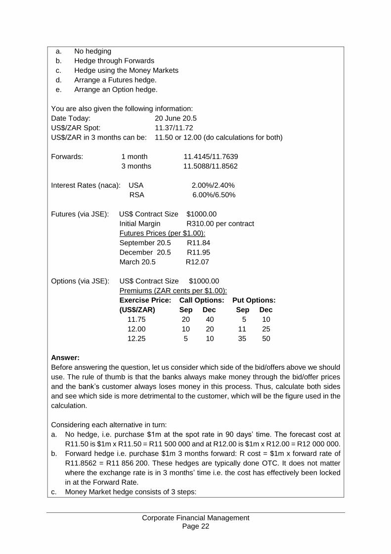
A South African company needs to pay its US supplier $1 million in 3 months’ time. You
have been asked by the company to consider five possible choices:
Corporate Financial Management Page 22
a. No hedging
b. Hedge through Forwards
c. Hedge using the Money Markets
d. Arrange a Futures hedge.
e. Arrange an Option hedge.
You are also given the following information:
Date Today: 20 June 20.5
US$/ZAR Spot: 11.37/11.72
US$/ZAR in 3 months can be: 11.50 or 12.00 (do calculations for both)
Forwards: 1 month 11.4145/11.7639
3 months 11.5088/11.8562
Interest Rates (naca): USA 2.00%/2.40%
RSA 6.00%/6.50%
Futures (via JSE): US$ Contract Size $1000.00
Initial Margin R310.00 per contract
Futures Prices (per $1.00):
September 20.5 R11.84
December 20.5 R11.95
March 20.5 R12.07
Options (via JSE): US$ Contract Size $1000.00
Premiums (ZAR cents per $1.00):
Exercise Price: Call Options: Put Options:
(US$/ZAR) Sep Dec Sep Dec
11.75 20 40 5 10
12.00 10 20 11 25
12.25 5 10 35 50
Answer:
Before answering the question, let us consider which side of the bid/offers above we should
use. The rule of thumb is that the banks always make money through the bid/offer prices
and the bank’s customer always loses money in this process. Thus, calculate both sides
and see which side is more detrimental to the customer, which will be the figure used in the
calculation.
Considering each alternative in turn:
a. No hedge, i.e. purchase $1m at the spot rate in 90 days’ time. The forecast cost at
R11.50 is $1m x R11.50 = R11 500 000 and at R12.00 is $1m x R12.00 = R12 000 000.
b. Forward hedge i.e. purchase $1m 3 months forward: R cost = $1m x forward rate of
R11.8562 = R11 856 200. These hedges are typically done OTC. It does not matter
where the exchange rate is in 3 months’ time i.e. the cost has effectively been locked
in at the Forward Rate.
c. Money Market hedge consists of 3 steps:
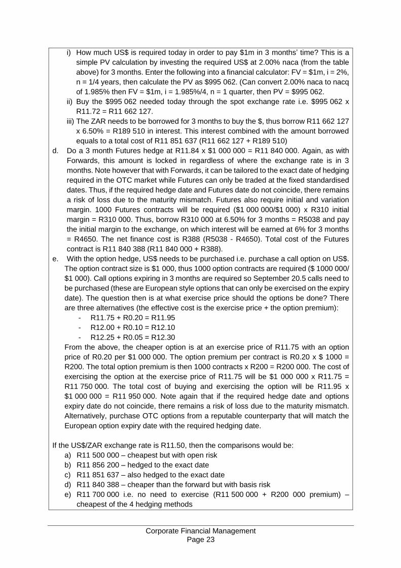
Corporate Financial Management Page 23
i) How much US$ is required today in order to pay $1m in 3 months’ time? This is a
simple PV calculation by investing the required US$ at 2.00% naca (from the table
above) for 3 months. Enter the following into a financial calculator: FV = $1m, i = 2%,
n = 1/4 years, then calculate the PV as $995 062. (Can convert 2.00% naca to nacq
of 1.985% then FV = $1m, i = 1.985%/4, n = 1 quarter, then PV = $995 062.
ii) Buy the $995 062 needed today through the spot exchange rate i.e. $995 062 x
R11.72 = R11 662 127.
iii) The ZAR needs to be borrowed for 3 months to buy the $, thus borrow R11 662 127
x 6.50% = R189 510 in interest. This interest combined with the amount borrowed
equals to a total cost of R11 851 637 (R11 662 127 + R189 510)
d. Do a 3 month Futures hedge at R11.84 x $1 000 000 = R11 840 000. Again, as with
Forwards, this amount is locked in regardless of where the exchange rate is in 3
months. Note however that with Forwards, it can be tailored to the exact date of hedging
required in the OTC market while Futures can only be traded at the fixed standardised
dates. Thus, if the required hedge date and Futures date do not coincide, there remains
a risk of loss due to the maturity mismatch. Futures also require initial and variation
margin. 1000 Futures contracts will be required ($1 000 000/$1 000) x R310 initial
margin = R310 000. Thus, borrow R310 000 at 6.50% for 3 months = R5038 and pay
the initial margin to the exchange, on which interest will be earned at 6% for 3 months
= R4650. The net finance cost is R388 (R5038 - R4650). Total cost of the Futures
contract is R11 840 388 (R11 840 000 + R388).
e. With the option hedge, US$ needs to be purchased i.e. purchase a call option on US$.
The option contract size is $1 000, thus 1000 option contracts are required ($ 1000 000/
$1 000). Call options expiring in 3 months are required so September 20.5 calls need to
be purchased (these are European style options that can only be exercised on the expiry
date). The question then is at what exercise price should the options be done? There
are three alternatives (the effective cost is the exercise price + the option premium):
- R11.75 + R0.20 = R11.95
- R12.00 + R0.10 = R12.10
- R12.25 + R0.05 = R12.30
From the above, the cheaper option is at an exercise price of R11.75 with an option
price of R0.20 per $1 000 000. The option premium per contract is R0.20 x $ 1000 =
R200. The total option premium is then 1000 contracts x R200 = R200 000. The cost of
exercising the option at the exercise price of R11.75 will be $1 000 000 x R11.75 =
R11 750 000. The total cost of buying and exercising the option will be R11.95 x
$1 000 000 = R11 950 000. Note again that if the required hedge date and options
expiry date do not coincide, there remains a risk of loss due to the maturity mismatch.
Alternatively, purchase OTC options from a reputable counterparty that will match the
European option expiry date with the required hedging date.
If the US$/ZAR exchange rate is R11.50, then the comparisons would be:
a) R11 500 000 – cheapest but with open risk
b) R11 856 200 – hedged to the exact date
c) R11 851 637 – also hedged to the exact date
d) R11 840 388 – cheaper than the forward but with basis risk
e) R11 700 000 i.e. no need to exercise (R11 500 000 + R200 000 premium) –
cheapest of the 4 hedging methods

Corporate Financial Management Page 24
If the US$/ZAR exchange rate is R12.00, then the comparisons would be:
a) R12 000 000 – most expensive
b) R11 856 200 – hedged to the exact date
c) R11 851 637 – also hedged to the exact date
d) R11 840 388 – cheapest but with basis risk
e) R11 950 000 (Exercised at R11.75 = R11 750 000 + R200 000 premium) – most
expensive of the 4 hedging methods but with upside potential
Comparing the five alternatives above the cheapest and the most expensive is not to hedge
at all but it is the riskiest – (a). The forward hedge (b) removes all uncertainty by fixing the
Exchange Rate now to the exact required hedging date. The Money Market hedge (c) is a
very close approximation of (b) as it should be, given that both are hedges to the exact date
and dependent on the same pricing drivers. Always calculate both and choose the cheapest
one. Futures (d) can be very attractive due to their standardised nature, tradability and
attractive pricing but they are not tailored for bespoke hedging dates and can leave the
hedger with basis risk. Options provide the hedger with “insurance” protection through the
payment of the premium while enjoying the upside, should the exchange rate move in a
favourable direction. In summary, (a) is too risky, (b to d) are used if the hedger is fairly
convinced or concerned that the exchange rate will deteriorate and (e) is used if the hedger
requires protection against a deterioration of the exchange rate but would also like to benefit
from a favourable move in the exchange rate.
Note that if the option premium above was quoted per ZAR1.00, then the $1m must first be
converted to its ZAR equivalent at the current spot rate (re: the premium is payable now)
and then multiplied by the ZAR option premium.
31. Replace the formula for Standard Deviation on page 400 with the formula below: Standard deviation is
N
X)(Xs
2
i
And the variance is s2
FORMULAE Note: these formulae are supplied in the examination paper (without the
keys). You are not expected to know them by heart, but you must be able to use and
apply them where necessary.
Corporate Financial Management Page 25
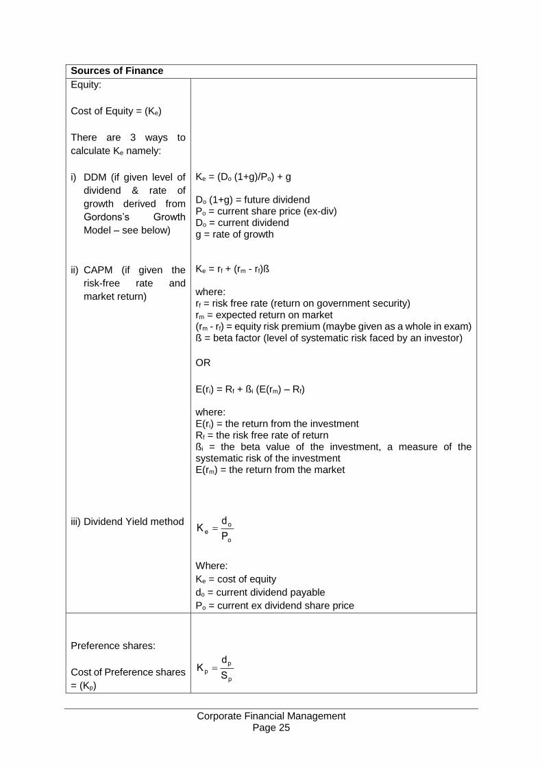
Sources of Finance
Equity:
Cost of Equity = (Ke)
There are 3 ways to
calculate Ke namely:
i) DDM (if given level of
dividend & rate of
growth derived from
Gordons’s Growth
Model – see below)
ii) CAPM (if given the
risk-free rate and
market return)
iii) Dividend Yield method
Ke = (Do (1+g)/Po) + g Do (1+g) = future dividend Po = current share price (ex-div) Do = current dividend g = rate of growth Ke = rf + (rm - rf)ß where: rf = risk free rate (return on government security) rm = expected return on market (rm - rf) = equity risk premium (maybe given as a whole in exam) ß = beta factor (level of systematic risk faced by an investor)
OR
E(ri) = Rf + ßi (E(rm) – Rf) where: E(ri) = the return from the investment Rf = the risk free rate of return ßi = the beta value of the investment, a measure of the systematic risk of the investment E(rm) = the return from the market
o
oe
P
dK
Where:
Ke = cost of equity
do = current dividend payable
Po = current ex dividend share price
Preference shares:
Cost of Preference shares
= (Kp)
p
p
pS
dK
Corporate Financial Management Page 26
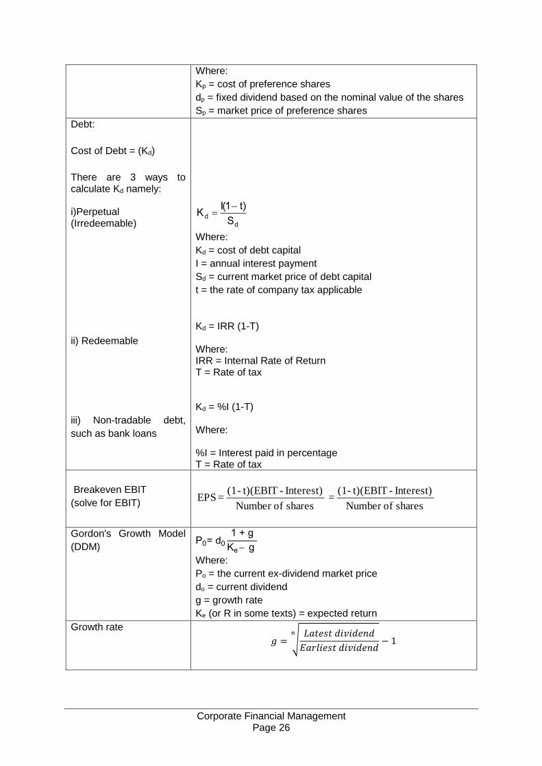
Where:
Kp = cost of preference shares
dp = fixed dividend based on the nominal value of the shares
Sp = market price of preference shares
Debt:
Cost of Debt = (Kd)
There are 3 ways to calculate Kd namely: i)Perpetual (Irredeemable)
ii) Redeemable
iii) Non-tradable debt,
such as bank loans
d
dS
t1IK
)(
Where:
Kd = cost of debt capital
I = annual interest payment
Sd = current market price of debt capital
t = the rate of company tax applicable
Kd = IRR (1-T) Where: IRR = Internal Rate of Return T = Rate of tax Kd = %I (1-T) Where: %I = Interest paid in percentage T = Rate of tax
Breakeven EBIT
(solve for EBIT)
shares ofNumber
Interest) - t)(EBIT-(1 = EPS
shares ofNumber
Interest) - t)(EBIT-(1 =
Gordon's Growth Model
(DDM) P0= d0
1 + g
Ke g
Where:
Po = the current ex-dividend market price
do = current dividend
g = growth rate
Ke (or R in some texts) = expected return
Growth rate
𝑔 = √𝐿𝑎𝑡𝑒𝑠𝑡 𝑑𝑖𝑣𝑖𝑑𝑒𝑛𝑑
𝐸𝑎𝑟𝑙𝑖𝑒𝑠𝑡 𝑑𝑖𝑣𝑖𝑑𝑒𝑛𝑑
𝑛
− 1
Corporate Financial Management Page 27
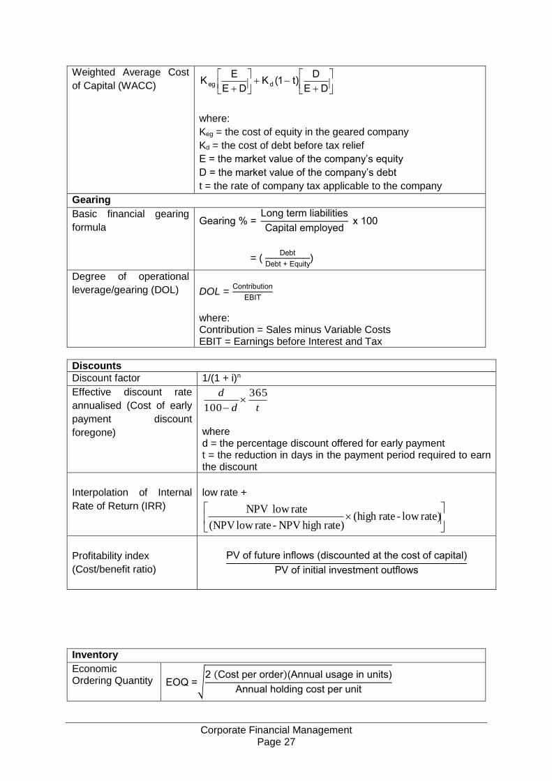
Weighted Average Cost
of Capital (WACC)
DE
Dt1K
DE
EK deg )(
where:
Keg = the cost of equity in the geared company
Kd = the cost of debt before tax relief
E = the market value of the company’s equity
D = the market value of the company’s debt
t = the rate of company tax applicable to the company
Gearing
Basic financial gearing
formula Gearing % =
Long term liabilities
Capital employed x 100
= ( Debt
Debt + Equity)
Degree of operational
leverage/gearing (DOL)
DOL = Contribution
EBIT
where: Contribution = Sales minus Variable Costs EBIT = Earnings before Interest and Tax
Discounts
Discount factor 1/(1 + i)n
Effective discount rate
annualised (Cost of early
payment discount
foregone)
td
d 365
100
where d = the percentage discount offered for early payment t = the reduction in days in the payment period required to earn the discount
Interpolation of Internal
Rate of Return (IRR)
low rate +
rate) low - ratehigh (
rate)high NPV - rate low (NPV
rate low NPV
Profitability index
(Cost/benefit ratio)
PV of future inflows (discounted at the cost of capital)
PV of initial investment outflows
Inventory
Economic Ordering Quantity EOQ =√
2 (Cost per order)(Annual usage in units)
Annual holding cost per unit
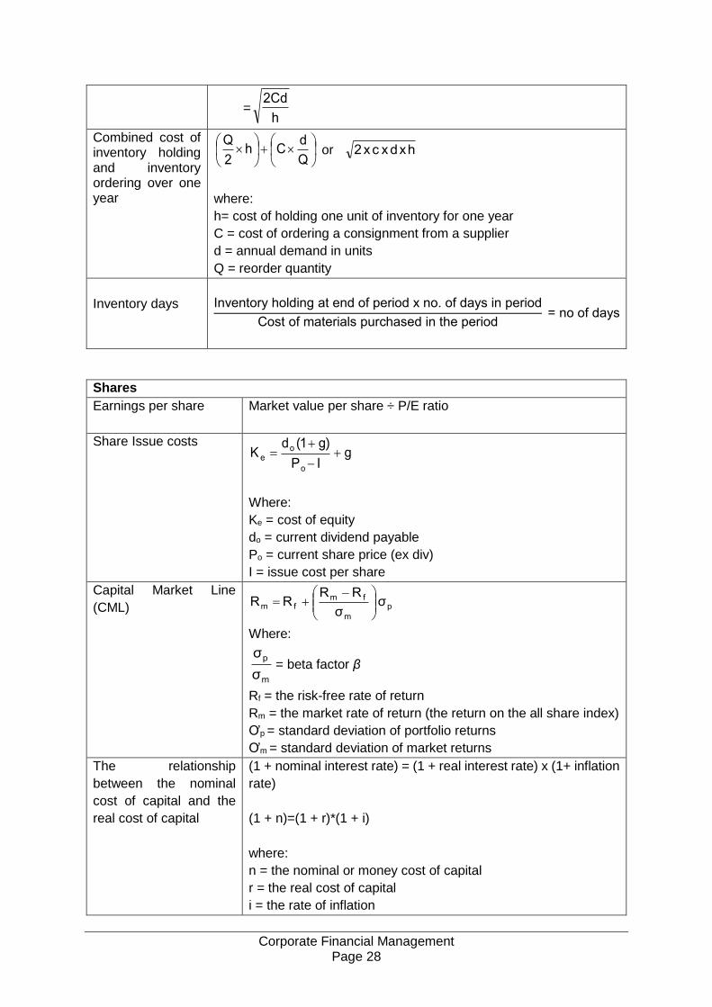
Corporate Financial Management Page 28
=h
Cd2
Combined cost of inventory holding and inventory ordering over one year
Q
dCh
2
Q or hxdxcx2
where:
h= cost of holding one unit of inventory for one year
C = cost of ordering a consignment from a supplier
d = annual demand in units
Q = reorder quantity
Inventory days
Inventory holding at end of period x no. of days in period
Cost of materials purchased in the period = no of days
Shares
Earnings per share Market value per share ÷ P/E ratio
Share Issue costs g
I P
g1dK
o
oe
)(
Where:
Ke = cost of equity
do = current dividend payable
Po = current share price (ex div)
I = issue cost per share
Capital Market Line
(CML) p
m
fmfm σ
σ
RRRR
Where:
m
p
σ
σ= beta factor β
Rf = the risk-free rate of return
Rm = the market rate of return (the return on the all share index)
Ơp = standard deviation of portfolio returns
Ơm = standard deviation of market returns
The relationship
between the nominal
cost of capital and the
real cost of capital
(1 + nominal interest rate) = (1 + real interest rate) x (1+ inflation
rate)
(1 + n)=(1 + r)*(1 + i)
where:
n = the nominal or money cost of capital
r = the real cost of capital
i = the rate of inflation
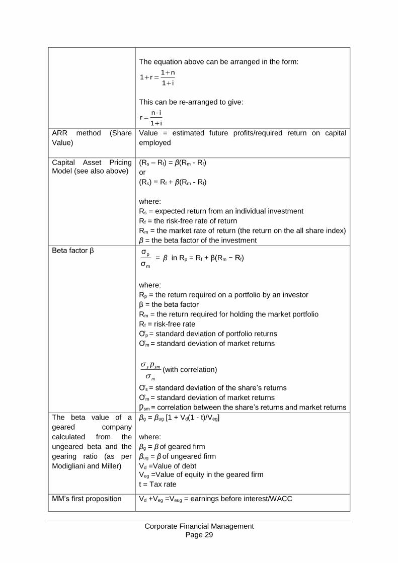
Corporate Financial Management Page 29
The equation above can be arranged in the form:
i1
n1r1
This can be re-arranged to give:
i1
i - nr
ARR method (Share
Value)
Value = estimated future profits/required return on capital
employed
Capital Asset Pricing Model (see also above)
(Rs – Rf) = β(Rm - Rf)
or
(Rs) = Rf + β(Rm - Rf)
where:
Rs = expected return from an individual investment
Rf = the risk-free rate of return
Rm = the market rate of return (the return on the all share index)
β = the beta factor of the investment
Beta factor β
m
p
σ
σ = β in Rp = Rf + β(Rm − Rf)
where:
Rp = the return required on a portfolio by an investor
β = the beta factor
Rm = the return required for holding the market portfolio
Rf = risk-free rate
Ơp = standard deviation of portfolio returns
Ơm = standard deviation of market returns
m
sms p
(with correlation)
Ơs = standard deviation of the share’s returns
Ơm = standard deviation of market returns
Ƿsm = correlation between the share’s returns and market returns
The beta value of a
geared company
calculated from the
ungeared beta and the
gearing ratio (as per
Modigliani and Miller)
βg = βug [1 + Vd(1 - t)/Veg]
where:
βg = β of geared firm
βug = β of ungeared firm
Vd =Value of debt Veg =Value of equity in the geared firm
t = Tax rate
MM’s first proposition Vd +Veg =Veug = earnings before interest/WACC
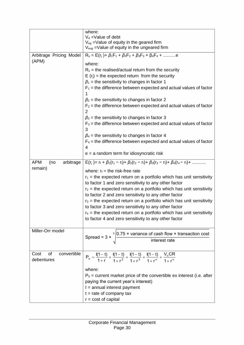
Corporate Financial Management Page 30
where: Vd =Value of debt Veg =Value of equity in the geared firm Veug =Value of equity in the ungeared firm
Arbitrage Pricing Model
(APM)
Rs = E(rj )+ β1F1 + β2F2 + β3F3 + β4F4 + ..........e
where:
Rs = the realised/actual return from the security
E (rj) = the expected return from the security
β1 = the sensitivity to changes in factor 1
F1 = the difference between expected and actual values of factor
1
β2 = the sensitivity to changes in factor 2
F2 = the difference between expected and actual values of factor
2
β3 = the sensitivity to changes in factor 3
F3 = the difference between expected and actual values of factor
3
β4 = the sensitivity to changes in factor 4
F4 = the difference between expected and actual values of factor
4
e = a random term for idiosyncratic risk
APM (no arbitrage
remain)
E(rj )= rf + β1(r1 − rf)+ β2(r2 − rf)+ β3(r3 − rf)+ β4(r4 − rf)+ ...........
where: rf = the risk-free rate
r1 = the expected return on a portfolio which has unit sensitivity
to factor 1 and zero sensitivity to any other factor
r2 = the expected return on a portfolio which has unit sensitivity
to factor 2 and zero sensitivity to any other factor
r3 = the expected return on a portfolio which has unit sensitivity
to factor 3 and zero sensitivity to any other factor
r4 = the expected return on a portfolio which has unit sensitivity
to factor 4 and zero sensitivity to any other factor
Miller-Orr model
Spread = 3 × √0.75 × variance of cash flow × transaction cost
interest rate
3
Cost of convertible
debentures n
n
n32or1
CRV
r1
t1I
r1
t1I
r1
t1I
r1
t1IP
)()()()(
where:
P0 = current market price of the convertible ex interest (i.e. after
paying the current year’s interest)
I = annual interest payment
t = rate of company tax
r = cost of capital

Corporate Financial Management Page 31
Vn = projected market value of the shares at year n, when
conversion
can take place
CR = conversion ratio
Mergers and Acquisitions
Exchange Ratio (ER)
based upon Market Value
ERT = Market Value per Target Company Share/Market Value
per Acquiring Company Share:
A
TT
MP
MPER
Exchange ratio with
synergistic benefits 1MP
ER MP premiumMarket
T
TA
Synergistic benefits are to
be allocated to the target
company’s shareholders AT
AMT
MP N
MVMVER
Where:
MVM = Market value of merged firm
MVA = Market value of acquiring firm
NT = Number of shares in issued share capital of target
company
MPA = Market price per share of acquiring company
Synergistic benefits are to
be retained by the
acquiring company )MV (MVN
N x MVER
TMT
AT
Where:
MVT = Market value of target firm
NA =Number of shares in issued share capital of acquiring
company
MVM = Market value of merged firm
Maximum exchange ratio
to be offered by the
acquiring company
ERmax=EPS𝑇
EPSA
+SE
EPSAN𝑇
Where: EPST = EPS of the target company
EPSA = EPS of the acquiring company
SE = Synergistic Earnings (annual earnings)
NT = Number of target company’s shares
NA = Number of acquiring company’s shares
Minimum exchange ratio
the target company can
accept
ERmin=EPS𝑇NA
SE + EPSANA
Sustainable Growth Rate
SGR =D
E (R − i)p + Rp
Corporate Financial Management Page 32
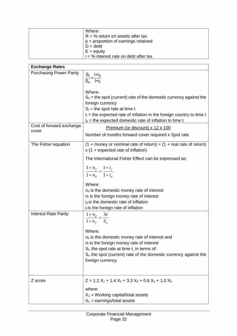
Where: R = % return on assets after tax p = proportion of earnings retained D = debt E = equity i = % interest rate on debt after tax
Exchange Rates
Purchasing Power Parity St
So
=I+id
I+if
Where: So = the spot (current) rate of the domestic currency against the
foreign currency
St = the spot rate at time t
if = the expected rate of inflation in the foreign country to time t
id = the expected domestic rate of inflation to time t. Cost of forward exchange cover
Premium (or discount) x 12 x 100
Number of months forward cover required x Spot rate
The Fisher equation (1 + money or nominal rate of return) = (1 + real rate of return)
x (1 + expected rate of inflation)
The International Fisher Effect can be expressed as:
d
f
d
f
i
i
n
n
1
1
1
1
Where:
nd is the domestic money rate of interest
nf is the foreign money rate of interest
id is the domestic rate of inflation
if is the foreign rate of inflation
Interest Rate Parity
of
d
S
St
n
n
1
1
Where:
nd is the domestic money rate of interest and
nf is the foreign money rate of interest
St, the spot rate at time t, in terms of:
So the spot (current) rate of the domestic currency against the
foreign currency
Z score
Z = 1.2 X1 + 1.4 X2 + 3.3 X3 + 0.6 X4 + 1.0 X5
where:
X1 = Working capital/total assets
X2 = earnings/total assets

Corporate Financial Management Page 33
X3 = earnings before tax and interest/total assets
X4 = market value of equity/book value of total debt
X5 = sales/total assets
Interest Rate Conversions
where: Ro = Rate of interest required (output) Ri = Rate of interest to be converted (input) Mo = Number of months required (output) Mi = Number of months corresponding with Ri above (input)
Beaver’s Ratio
(Default prediction)
Cash Flow from Operations
Total Debt
Financial Ratios
Current ratio = Current assets
Current liabilities
Quick ratio = Current assets – inventory
Current liabilities
Inventory turnover = Cost of sales/Purchases
Inventory
Inventory days =
Inventory x 365 Cost of sales/Purchases
Average collection = Accounts receivable x 365
Sales
Fixed asset turnover = Sales
Fixed assets
Asset turnover = Sales
Operating assets
Debt ratio = Debt
Total assets
Debt to equity = Total debt
Total equity
Times interest earned = EBIT
Interest
EBITDA coverage = EBIT + depreciation + amortisation
Interest
Fixed charge coverage = EBIT + depreciation + amortisation + lease payments
Interest + lease payments
o
M
M
iio
M
MRR i
o
12x }1]))
12 x(1{[(
Corporate Financial Management Page 34
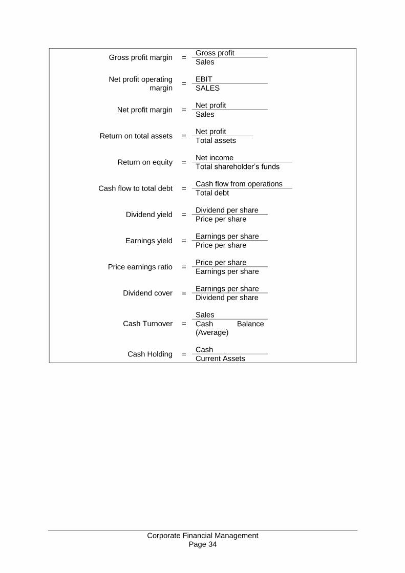
Gross profit margin = Gross profit
Sales
Net profit operating margin
= EBIT
SALES
Net profit margin = Net profit
Sales
Return on total assets = Net profit
Total assets
Return on equity = Net income
Total shareholder’s funds
Cash flow to total debt = Cash flow from operations
Total debt
Dividend yield = Dividend per share
Price per share
Earnings yield = Earnings per share
Price per share
Price earnings ratio = Price per share
Earnings per share
Dividend cover = Earnings per share
Dividend per share
Cash Turnover =
Sales
Cash Balance (Average)
Cash Holding = Cash
Current Assets