www.sciencemag.org/cgi/content/full/329/5999/1616/DC1

Supporting Online Material for

Reaction-Diffusion Model as a Framework for Understanding Biological Pattern Formation

Shigeru Kondo* and Takashi Miura

*To whom correspondence should be addressed. E-mail: skondo@fbs.osaka-u.ac.jp

Published 24 September 2010, Science 329, 1616 (2010)

DOI: 10.1126/science.1179047

This PDF file includes:

SOM Text Figs. S1 to S5 References

Other Supporting Online Material for this manuscript includes the following: (available at www.sciencemag.org/cgi/content/full/329/5999/1616/DC1)

Computer simulation

Supplemental Information 1

This supplemental information consists of four sections,

1) Brief explanation of original RD model

Summary of the Turing’s original paper is explained without using mathematics.

2) Intuitive explanation of Turing instability (diffusion-driven instability) from

mathematical point of view

The most important and strange output of the RD model is its ability to generate

patterns without any pre-pattern. This section is a mathematical explanation of such

behavior of the system.

3) Guide to the RD model simulator and the Mathematical information related to the

simulation

A user-friendly simulator of RD model is provided as the supplemental material 2.

The program runs on the web browser. This section explains some important

mathematical information that is required to set the parameters.

1-1) Brief explanation of original RD model

Here, we describe the aim and the result of Turing’s study briefly. This information is

enough to give the rough image of the RD model to the biologists who are not familiar

to the theoretical models, but not enough for accurate understanding of the theory. For

the details of the mathematical analysis of the theory, please refer the original paper of

Turing or some specific textbooks. (See references in the main text)

Alan Mathison Turing (23 June 1912 – 7 June 1954) was an English mathematician,

logician, and computer scientist who is now recognized as one of the founder of

computer science. He is also famous by the fact that he played a definitive role in the

codebreaking of German naval cipher Enigma during the WW2. The paper titled “The

Chemical Basis of Morphogenesis” was written two years before his committing suicide

by an apple containing potassium cyanide. The reason why the mathematician Turing

got interested in the mechanism of biological morphogenesis is unknown. But, the

strategy he took to solve this biological question is certainly that of mathematician. For

Turing, the complex morphology of living things was the complex theorem of

mathematics to be solved by the basic axioms. He tried to solve the question of

morphogenesis by assembling well-known basic physical laws.

He selected chemical reaction and diffusion as the basis of his study, and analyzed the

behavior of a hypothetical system (reaction-diffusion system) composed of two kinds of

diffusible and interacting chemicals. In 1950’s, biochemistry was the forefront of

biological science and the detailed information of cell biology was unknown yet.

Therefore it is quite reasonable that Turing selected reaction and diffusion as the basis

of his analysis. If he were alive now, he might have analyzed a system of cells

interacting by the ligands and receptors that is more familiar for the biologist of present

day. Here, we use a hypothetical system in which cells release and react to two kinds of

ligands. (Supplemental figure 1) Of course, this alteration does not change the essence

of Turing’s study.

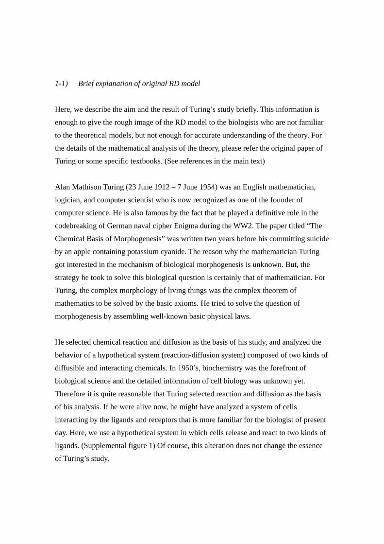
Supplemental figure 1: Schematic drawing of the hypothetical system assumed in this text.

Supplemental figure 1 shows the system we are going to analyze. Each cell produces

two diffusible ligands, u and v, and has the receptors for them. The released ligands

diffuse in the space around the cells at their specific diffusion constants, bind to the

receptor and enhance (or repress) the production of themselves.

Following equation represent the rate of concentration change at each position.

∂u∂t

= F(u,v) − duv + DuΔu

∂v∂t

= G(u,v) − dvv + DvΔv

Supplemental figure 2: Mathematical description of the condition shown in supplemental figure 1, and the

meaning of what each column represents.

Here, x and y are the local concentration of ligands U and V at each position. F and G

are the functions governing the production rates. du and dv are the degradation rates.

Replacing F and G by following linear function, we get the partial differential equation

identical to that of Turing’s original paper.

F(u,v) − duu = auu + buv + cu

G(u,v) − dvv = avu + bvv + cv

He solved this differential equation, and found that this system can take several

interesting dynamic states (figure 3) depending on the values of the parameter.

Followings are the 6 different cases described in the Turing’s paper. (Please refer the

main text.)

Supplemental figure 3: Solutions of the Turing’s reaction-diffusion equation. The system converges one

of these states shown in above. Note that case IV needs three (or more) morphogens.

As above 6 cases are the solutions of differential equation, boundary condition

influences the resulting pattern. (patterns shown in FigS1 are the cases with periodic

boundary condition) Giving a very specific boundary condition is very similar to

having a pre-pattern in the real system. In case I, if the concentration of morphogen U

is kept high at the end of the field, the resulting pattern becomes a gradient of a single

peak. This is identical to that of morphogen gradient model.

The most important finding of the Turing’s study is that this simple system can develop

the spatial pattern. This behavior of the system is apparently against our intuition. To

explain why such strange phenomenon occurs in this system, a fully mathematical

explanation is required. But, with following narrative explanation, it is possible to get

the rough image of it. The key is that the difference of the diffusion constant of activator

(u) and inhibitor (v).

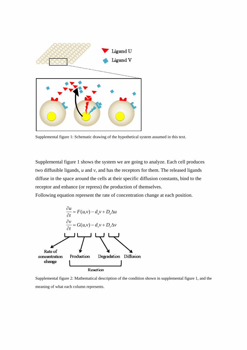
Supplemental figure 4: the schematic representation of the process of Stationary pattern formation (Case

VI)

Graph1 shows the initial condition of the system. Suppose that the concentration of the

activator is relatively higher than in other regions by random fluctuation. By the

self-enhancing property of the activator, the concentration of activator increases at the

center region (graph2), followed by the increase of inhibitor at the neighboring region A.

As the diffusion rate of inhibitor is much larger than that of the activator, substantial

amounts of inhibitor move toward the lateral regions. This depresses the activator

function, resulting in the decrease of the activator concentration there (graph3).

Decrease of activator causes the decrease of inhibitor in the wider region (graph4). At

the region B, as inhibitor concentration is gotten lower, activator becomes relatively

dominant than inhibitor. This situation is enough to start the local self activation at

region B (graph5).

This process is visible with the simulator provided as the supplemental material 2.

Computer simulation is one of the best ways to gain insight into the pattern-generating

power of the Turing mechanism.

1-2) Intuitive explanation Turing instability (diffusion-driven instability) from

mathematical point of view

Here we give a very intuitive explanation of Turing instability (diffusion-driven

instability) from mathematical point of view. For full detail of the analysis, the reader

should consult Murray (2003).

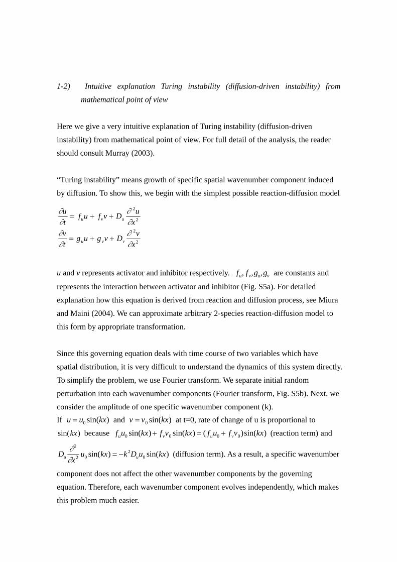
“Turing instability” means growth of specific spatial wavenumber component induced

by diffusion. To show this, we begin with the simplest possible reaction-diffusion model

2

2

2

2

xvDvgug

tv

xuDvfuf

tu

vvu

uvu

∂∂

∂∂

∂∂

∂∂

++=

++=

u and v represents activator and inhibitor respectively. fu, fv,gu,gv are constants and

represents the interaction between activator and inhibitor (Fig. S5a). For detailed

explanation how this equation is derived from reaction and diffusion process, see Miura

and Maini (2004). We can approximate arbitrary 2-species reaction-diffusion model to

this form by appropriate transformation.

Since this governing equation deals with time course of two variables which have

spatial distribution, it is very difficult to understand the dynamics of this system directly.

To simplify the problem, we use Fourier transform. We separate initial random

perturbation into each wavenumber components (Fourier transform, Fig. S5b). Next, we

consider the amplitude of one specific wavenumber component (k). If and at t=0, rate of change of u is proportional to

because

u = u0 sin(kx) v = v0 sin(kx)

sin(kx) fuu0 sin(kx)+ fvv0 sin(kx) = ( fuu0 + fvv0)sin(kx) (reaction term) and

Du∂ 2

∂x 2 u0 sin(kx) = −k 2Duu0 sin(kx) (diffusion term). As a result, a specific wavenumber

component does not affect the other wavenumber components by the governing

equation. Therefore, each wavenumber component evolves independently, which makes

this problem much easier.

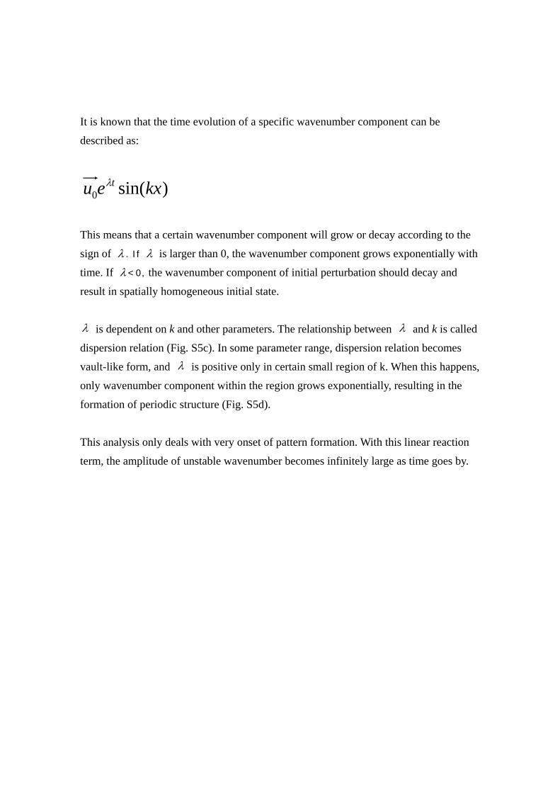
It is known that the time evolution of a specific wavenumber component can be

described as:

u0eλt sin(kx)

This means that a certain wavenumber component will grow or decay according to the

sign of λ . If λ is larger than 0, the wavenumber component grows exponentially with

time. If λ<0, the wavenumber component of initial perturbation should decay and

result in spatially homogeneous initial state.

λ is dependent on k and other parameters. The relationship between λ and k is called

dispersion relation (Fig. S5c). In some parameter range, dispersion relation becomes

vault-like form, and λ is positive only in certain small region of k. When this happens,

only wavenumber component within the region grows exponentially, resulting in the

formation of periodic structure (Fig. S5d).

This analysis only deals with very onset of pattern formation. With this linear reaction

term, the amplitude of unstable wavenumber becomes infinitely large as time goes by.

Supplemental figure 5

a. Relationship between activator-inhibitor interaction and model parameter. b. Initial distribution of u or

v. c. Dispersion relation, d. Time evolution of each wavenumber component.

1-3) Guide to the RD model simulator and the Mathematical information related to

the simulation

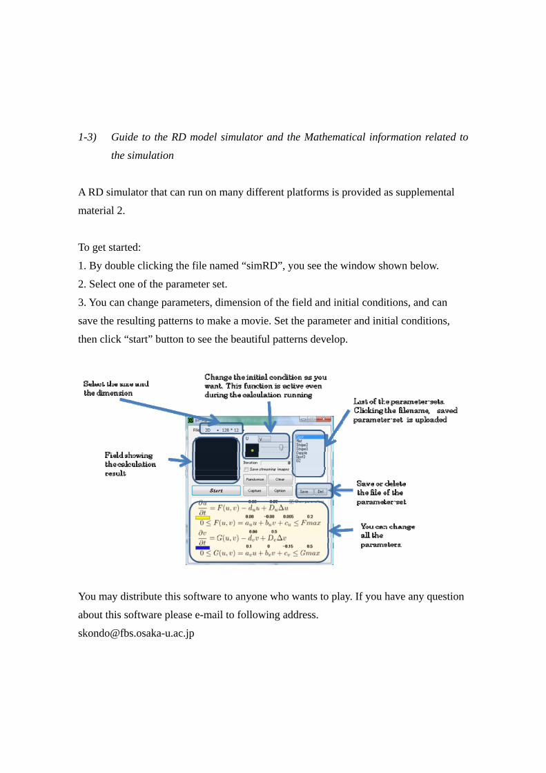
A RD simulator that can run on many different platforms is provided as supplemental

material 2.

To get started:

1. By double clicking the file named “simRD”, you see the window shown below.

2. Select one of the parameter set.

3. You can change parameters, dimension of the field and initial conditions, and can

save the resulting patterns to make a movie. Set the parameter and initial conditions,

then click “start” button to see the beautiful patterns develop.

You may distribute this software to anyone who wants to play. If you have any question

about this software please e-mail to following address.

skondo@fbs.osaka-u.ac.jp

Followings are the important information about the parameters and resulting pattern.

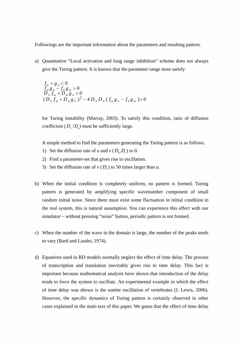
a) Quantitative “Local activation and long range inhibition” scheme does not always

give the Turing pattern. It is known that the parameter range must satisfy

f u + g v < 0f u g v − f v g u > 0D v f u + D u g v > 0( D v f u + D u g v )2 − 4 D u D v ( f u g v − f v g u )> 0

for Turing instability (Murray, 2003). To satisfy this condition, ratio of diffusion coefficient ( Dv /Du) must be sufficiently large.

A simple method to find the parameters generating the Turing pattern is as follows. 1) Set the diffusion rate of u and v ( Du,Dv ) to 0.

2) Find a parameter-set that gives rise to oscillation. 3) Set the diffusion rate of v ( Dv ) to 50 times larger than u.

b) When the initial condition is completely uniform, no pattern is formed. Turing

pattern is generated by amplifying specific wavenumber component of small

random initial noise. Since there must exist some fluctuation in initial condition in

the real system, this is natural assumption. You can experience this effect with our

simulator – without pressing “noise” button, periodic pattern is not formed.

c) When the number of the wave in the domain is large, the number of the peaks tends

to vary (Bard and Lauder, 1974).

d) Equations used in RD models normally neglect the effect of time delay. The process

of transcription and translation inevitably gives rise to time delay. This fact is

important because mathematical analysis have shown that introduction of the delay

tends to force the system to oscillate. An experimental example in which the effect

of time delay was shown is the somite oscillation of vertebrates (J. Lewis, 2006).

However, the specific dynamics of Turing pattern is certainly observed in other

cases explained in the main text of this paper. We guess that the effect of time delay

is negligible if the time scale of pattern formation is much longer than transcription

or translation.

e) Numerical simulation does not always show correct behavior due to numerical error.

For example, we can reduce computation time by increasing timestep (dt) and unit

length of the field (dx). But the change of these parameters often results in artificial

oscillation or burst of calculation. Intuitive explanation of this error is as follows:

diffusion process represents flow of diffusible molecule from high concentration

region to low concentration region. However, if we take dt too large, molecule

concentration in initially high concentration region becomes lower than originally

low concentration region. So we recommend that these parameters left to be as it is

until the player gets accustomed to numeral simulations.

References:

1) J. Murray, Mathematical Biology, 4th edition. (Springer-Verlag, Berlin, 2003).

2) Miura, T. & Maini, P. K., Periodic pattern formation in reaction-diffusion systems: an

introduction for numerical simulation. Anat Sci Int, 79, 112-23 (2004)

3) E.A. Gaffney, N.A.M. Monk, Gene expression time delays and Turing pattern

formation systems, Bulletin Mathematical Biology, 68, 99-130 (2006)

4) Lewis, J. Autoinhibition with transcriptional delay: a simple mechanism for the

zebrafish somitogenesis oscillator. Curr. Biol. 13, 1398–-1408 (2003).

5) Bard, J. & Lauder I, How well does Turing’s theory of Morphogenesis work? J.

theor. biol. 45, 501-531 (1974).