systematic identification of high crash locations

SYSTEMATIC IDENTIFICATION

OF HIGH CRASH LOCATIONS

MAY 2001

Sponsored by the Iowa Department of Transportationand the Iowa Highway Research Board

Iowa DOT Project TR-442CTRE Management Project 00-59

Center for Transportation

Research and Education

CTRE

FINAL REPORT

CTRE’s mission is to develop and implement innovative methods, materials, and technologiesfor improving transportation efficiency, safety, and reliability while improving the learningenvironment of students, faculty, and staff in transportation-related fields.

The opinions, findings, and conclusions expressed in this publication are those of theauthors and not necessarily those of the Iowa Department of Transportation.

��

�INAL �EPORT

��

��

� ��

� ��

��

��

�� !��"

��

��

#�� $��

%��

��

!�� !& !��

'��

'�� (��

��

��

�� ! ��)

��

��* +� ��*�

��

+��

�� " � � ��

�� $�� +��

�� ,� ��*�� -../

��

� �� " � � ��

� ��

��

�� (�� *�� 00-12

�� !��

��" �� #

/203 �� 4�� 5300

�� 10030-675/

�� 8 131-/2.-6305

'�98 131-/2.-0.7:

��8;;��&��&�� &��

�AY $%%&�

iii

TABLE OF CONTENTS

EXECUTIVE SUMMARY ........................................................................................................... ix

1 INTRODUCTION .....................................................................................................................1

2 LITERATURE REVIEW ..........................................................................................................32.1 Horizontal Curves .............................................................................................................32.2 Fixed-Object Crashes........................................................................................................42.3 Head-on Crashes Due to Crossing Centerline ..................................................................52.4 Intersections Along Rural Four-Lane Expressways .........................................................6

3 METHODOLOGY ....................................................................................................................93.1 General Assumptions and Effects.....................................................................................93.2 Identification of High Crash Locations ..........................................................................10

3.2.1 Horizontal Curves ...............................................................................................113.2.2 Fixed-Object Crashes..........................................................................................153.2.3 Rural Four-Lane Expressway Intersections........................................................163.2.4 Head-on Crashes Due to Crossing Centerline ....................................................183.2.5 Urban Four-Lane Undivided Corridors ..............................................................19

3.3 Causal Factors and Regression Analysis ........................................................................203.3.1 Head-on Crashes Due to Crossing Centerline ....................................................213.3.2 Fixed-Object Crashes..........................................................................................223.3.3 Horizontal Curves ...............................................................................................23

4 RESULTS ................................................................................................................................254.1 High Crash Locations .....................................................................................................25

4.1.1 Horizontal Curves ...............................................................................................254.1.2 Fixed-Object Crashes..........................................................................................304.1.3 Rural Four-Lane Expressway Intersections........................................................384.1.4 Head-on Crashes Due to Crossing Centerline ....................................................424.1.5 Urban Four-Lane Undivided Corridors ..............................................................45

4.2 Causal Factors and Regression Analysis ........................................................................514.2.1 Head-on Crashes Due to Crossing Centerline ....................................................514.2.2 Fixed-Object Crashes..........................................................................................554.2.3 Horizontal Curves ...............................................................................................58

5 CONCLUSIONS AND RECOMMENDATIONS ..................................................................61

ACKNOWLEDGMENTS .............................................................................................................63

REFERENCES ..............................................................................................................................65

APPENDIX A: IOWA DOT HIGH CRASH LOCATION RANKING PROCEDURE

APPENDIX B: HORIZONTAL CURVE IDENTIFICATION STRATEGIES

APPENDIX C: HORIZONTAL CURVE IDENTIFICATION METHODOLOGY

APPENDIX D: PROCEDURES

v

LIST OF TABLES

Table 1 Potential Study Topics .................................................................................................... 11Table 2 Curve Geometry Closed Form Solution ......................................................................... 15Table 3 Selected Roadway Characteristics .................................................................................. 21Table 4 High Crash Locations—Rural Curves ............................................................................ 26Table 5 High Crash Locations—Rural Curves (Descriptions) .................................................... 27Table 6 High Crash Locations—Secondary Road Curves (Story County).................................. 29Table 7 High Crash Locations—Collisions with Fixed Objects.................................................. 31Table 8 High Crash Locations—Collisions with Fixed Objects (Descriptions).......................... 32Table 9 High Crash Locations—Collisions with Utility Poles.................................................... 34Table 10 High Crash Locations—Collisions with Utility Poles (Descriptions).......................... 35Table 11 High Crash Locations—Rural Four-Lane Intersections ............................................... 39Table 12 High Crash Locations—Rural Four-Lane Intersections (Descriptions) ....................... 40Table 13 High Crash Locations—Head-on Crashes.................................................................... 42Table 14 High Crash Locations—Head-on Crashes (Descriptions) ............................................ 43Table 15 High Crash Locations—Four-Lane Undivided Corridors ............................................ 45Table 16 High Crash Locations—Four-Lane Undivided Corridors (Descriptions) .................... 46Table 17 High Crash Locations—Partial Four-Lane Undivided Corridors................................. 48Table 18 High Crash Locations—Partial Four-Lane Undivided Corridors (Descriptions) ......... 49Table 19 Segment Characteristics for Head-on Crashes.............................................................. 52Table 20 Differences in Head-on Crash Rate Means (t-statistic) ................................................ 52Table 21 Head-on Crash Rate Model for US Highways.............................................................. 53Table 22 Head-on Crash Rate Model for Iowa Highways........................................................... 53Table 23 Head-on Crash Rate Model for Farm-to-Market Roads ............................................... 54Table 24 Head-on Crash Rate Model for Local Roads................................................................ 55Table 25 Segment Characteristics for Fixed-Object Crashes ...................................................... 55Table 26 Differences in Fixed-Object Crash Rate Means (t-statistic) ......................................... 56Table 27 Fixed-Object Crash Rate Model for Interstate Highways ............................................ 56Table 28 Fixed-Object Crash Rate Model for US Highways ...................................................... 56Table 29 Fixed-Object Crash Rate Model for Iowa Highways ................................................... 57Table 30 Fixed-Object Crash Rate Model for Farm-to-Market Roads........................................ 58Table 31 Fixed-Object Crash Rate Model for Local Roads ........................................................ 58Table 32 Horizontal Curve Crash Rate Model ............................................................................ 59

vii

LIST OF FIGURES

Figure 1 Data Flow Diagram ......................................................................................................... 2Figure 2 High Crash Locations —Rural Curves.......................................................................... 28Figure 3 High Crash Location—Rural Curves (No. 2)................................................................ 28Figure 4 High Crash Locations—Secondary Road Curves (Story County) ................................ 30Figure 5 High Crash Locations—Collisions with Fixed Objects ................................................ 33Figure 6 High Crash Locations—Collisions with Fixed Objects (No. 1).................................... 33Figure 7 High Crash Locations—Collisions with Utility Poles .................................................. 36Figure 8 High Crash Locations—Collisions with Utility Poles, Des Moines Area (“A”) .......... 36Figure 9 High Crash Locations—Collisions with Utility Poles, Muscatine Area (“B”) ............. 37Figure 10 High Crash Locations—Collisions with Utility Poles, Davenport Area (“C”) ........... 37Figure 11 High Crash Locations—Collisions with Utility Poles (No. 1) .................................... 38Figure 12 High Crash Locations—Rural Four-Lane Intersections.............................................. 41Figure 13 High Crash Locations—Rural Four-Lane Intersections (No. 1) ................................. 41Figure 14 High Crash Locations—Head-on Crashes................................................................... 44Figure 15 High Crash Locations—Head-on Crashes (No. 1) ...................................................... 44Figure 16 High Crash Locations—Four-Lane Undivided Corridors........................................... 47Figure 17 High Crash Locations—Partial Four-Lane Undivided Corridors ............................... 50Figure 18 High Crash Locations—Four-Lane Undivided Corridor (No. 1)................................ 50Figure 19 High Crash Locations—Four-Lane Undivided Corridor (No. 2) and Component

Segments ................................................................................................................................ 51Figure 20 Farm-to-Market Roads with Potentially Higher Head-on Crash Rates....................... 54Figure 21 US Highways with Potentially Higher Fixed-Object Crash Rates.............................. 57

ix

EXECUTIVE SUMMARY

Background and Objective

Federal and state policy makers increasingly emphasize the need to reduce highway crash rates.This emphasis is demonstrated in Iowa’s recently released draft Iowa Strategic Highway SafetyPlan and by the U.S. Department of Transportation’s placement of “improved transportationsafety” at the top of its list of strategic goals. Thus, finding improved methods to enhancehighway safety has become a top priority at highway agencies.

The objective of this project is to develop tools and procedures by which Iowa engineers canidentify potentially hazardous roadway locations and designs, and to demonstrate the utility ofthese tools by developing candidate lists of high crash locations in the State. An initial task,building an integrated database to facilitate the tools and procedures, is an important product, inand of itself. Accordingly, the Iowa Department of Transportation (Iowa DOT) GeographicInformation Management System (GIMS) and Geographic Information System AccidentAnalysis and Location System (GIS-ALAS) databases were integrated with available digitalimagery. (The GIMS database contains roadway characteristics, e.g., lane width, surface andshoulder type, and traffic volume, for all public roadways. GIS-ALAS records include data, e.g.,vehicles, drivers, roadway conditions, and the crash severity, for crashes occurring on publicroadways during then past 10 years.)

Procedure

Using the GIMS and GIS-ALAS databases, high crash locations and relationships between crashrates and selected roadway design characteristics were identified. Based on input from county,state and consulting engineers, the project studied five crash types: (1) crashes on horizontalcurves, (2) fixed-object crashes, (3) rural four-lane expressway intersection crashes, (4) head-oncrashes (due to crossing the centerline), and (5) urban four-lane undivided corridor crashes.

Procedures were developed to integrate crash records and roadway characteristics (e.g., trafficvolumes, number of lanes) to estimate the crash rate on any segment of the Iowa roadwaynetwork and rank high crash locations using the Iowa DOT’s conventional procedure. (At thetime of this study, the Iowa DOT ranked high crash locations by frequency, rate and loss. Thethree rankings were averaged to provide a final list of high crash locations.) Using the integrateddatabase, statistical relationships between crash rates and roadway characteristics were thenestablished. The resulting statistical models identify significant roadway geometric factors incausation of certain crashes.

In this project, geographic information system (GIS) based procedures were developed tofacilitate the identification and analysis of elusive roadway criteria, e.g., curve radii, which arenot identified by crash records. A method was also developed for determining the most recentdaily entering vehicles at intersections and for reviewing and defining extents of location specificanalysis (e.g., corridors).

x

A key deliverable of this research is the development of a combined automated and manualapproach to identify curves. The strategy involved the application of a closed form solution toresolving curve radii and degree of curvature based on GIS-measured chord measurement(determination of curve radii from chord and length measurement typically involves a time-consuming iterative solution, which makes systematic analysis in a database difficult and timeconsuming).

Following a literature review to identify models relating crash rates and roadway characteristics,analysis of head-on and fixed-object crash data was conducted using a two-step process. First,descriptive statistics were obtained and comparisons were conducted for crash rates on differenttypes of facilities (interstate, US highway, etc.). Second, regression models were estimated forhead-on and fixed-object crash rates on different facilities to relate the crash rate to segmentattributes (e.g., number of lanes, pavement type, and speed limit). A regression analysis was alsoconducted to explain the relationship of curve length and radius to crash rate in Iowa.

Results

As expected, results indicate that head-on crash rates are higher on lower classification (e.g.,local and farm to market) highways. Rates are also affected by speed limit, terrain, shoulderwidth, shoulder type, and the pavement condition (international roughness index). For example,the results show that US and Iowa highways with higher speed limits have a lower head-on crashrate. While for a given facility, higher speed may result in more serious crashes, the finding isconsistent as high speed limit roads are typically designed to a higher geometric standard. Themodels also indicate that crash rates decrease with increasing values of total shoulder width (i.e.,the sum of inside and outside shoulder widths).

Also as would be expected, the analysis indicates that fixed-object crash rates are higher onlower classification (local and farm-to-market) highways. Terrain, type of pavement, shouldertype, the absence of median barriers, surface width, and number of lanes all tend to affect fixed-object crash rates on different types of highways. Not expected was the observation that, forinterstate highways, highway segments in flat and rolling terrain tend to have higher crash ratescompared to segments in hilly terrain. Similarly, segments with asphalt cement concretepavement surface tend to experience higher crash rates compared to other types of surfaces.Moreover, segments with paved shoulders have lower fixed-object crash rates, where assegments with no median barrier tend to have higher fixed-object crash rates. Many of theseobservations are correlated with overall design standards, and, probably due to the rare andcomplex causal nature of crashes, few of the relationships have strong statistical significance.Table ES.1 summarizes the statistically significant roadway geometric factors in causation of fix-object and head-on crashes at the 90 or 95 percent confidence level.

As was expected from previous studies, the analysis of curve-related crash data indicates that thedegree of curvature has a direct impact on crash rates on horizontal curves. Furthermore, themodel indicates that the crash rate on shorter curve lengths is significantly higher than the crashrate on longer curves. This is probably because sharp curves are usually shorter than mild curves(see Reinfurt et al., Analysis of Vehicle Operations on Horizontal Curves, TransportationResearch Record 1318).

xi

Conclusions and Recommendations

In Iowa, as in most states, highway engineering safety improvement programs are reactive. Inother words, safety countermeasures are applied to the roadway only after high crash rates havebeen observed. The objective of this project was to quantify the impact of highway geometry anddesign features on crash rates, enabling agencies to proactively identify and mitigate futureproblem areas.

The application of GIS in this project has enabled the research team to identify and analyzeroadway segments characterized by specific criteria that are not identified by conventional crashanalysis. Along the way, methods were developed for solving intermediate problems that willalso find utility at state DOTs (e.g., determining most recent daily entering vehicles atintersections and reviewing and defining extents or location specific analysis). Another usefulproduct is an improved corridor analysis methodology.

The project produced the following items:

• curve database for Iowa, with radii and length attributes• procedures for identifying high crash locations of five types• statistical models of the relationship between geometric features and crash rates• candidate lists (maps and tables) for improvement (Iowa top 30 lists) for five problem

types

Table ES.1 Statistically Significant Roadway Geometric Crash Causal Factors

Interstate US Hwy IA Hwy Farm-to-Market Local90%Conf.

95% Conf. 90% Conf. 95% Conf. 90% Conf. 95% Conf. 90% Conf. 95% Conf. 90% Conf. 95% Conf.

Flat terrain No barrier Flat terrain Combination pavement Earth/gravel shoulders ACC pavement Flat terrain ACC pavementACC pavement Surface width PCC pavement PCC pavement

Fixed-object Paved shoulders No of lanesRolling terrain Speed limitNo barrier

Flat terrain Speed limit Speed limit Total shoulder widthHead-on Total shoulder width Total shoulder width Unpaved shoulders

IRI

xii

1

1 INTRODUCTION

Federal and state policy makers increasingly emphasize the need to reduce highway crash rates.This emphasis can be witnessed at the state level in Iowa’s recently released draft Iowa StrategicHighway Safety Plan and at the federal level by the U.S. Department of Transportation’splacement of “improved transportation safety” at the top of its list of strategic goals (1, 2). Thus,finding improved methods to enhance highway safety has become a top priority at highwayagencies.

The purpose of the research project was to develop tools and procedures by which Iowaengineers can identify potentially hazardous roadway locations and designs. Through selectedcase studies and using a system of integrated geographically referenced databases, the projectidentified high crash locations and relationships between crash rates and roadway designcharacteristics.

This project engaged a variety of existing databases in geographically referenced environments.The Iowa crash records and the Iowa road base records were the principal databases used. Otherdata sources used included cartography files, aerial photos, and Roadware pavementmanagement centerline data. These databases were integrated to focus on safety analysis andmonitoring, resulting in a composite database in which the roadway characteristics leading toheightened crash rates could be determined.

An important feature of the research is that it interconnected databases that had not previouslybeen used together systematically to create a rich environment for conducting safety analyses.However, it is important to note that compiling the data sets needed for this project was possibleonly because of previous investments by the Iowa Department of Transportation (Iowa DOT) inthe development of multiple geographically referenced databases.

Furthermore, statistical analyses of crash data revealed the relationship between crash rates androadway design features, geometry, or other characteristics (e.g., speed limit, annual averagedaily traffic [AADT], surface type and condition). The resulting statistical models determined themost significant factors in causation of specific crashes. The identified contributing factors or“problem” types led to the determination of “problem” areas throughout the state. The graphicalrepresentation of the process is shown in a data flow diagram in Figure 1. By identifying designfeatures and/or characteristics that may lead to higher crash risk, it is hoped that engineers coulduse the results to proactively reduce such hazards in future roadway designs or eliminate them inexisting roadways.

This report consists of five chapters and four appendices. Chapter 1 is this brief introduction tothe research project. Chapter 2 reviews relevant articles and reports. The approached strategiesare documented in Chapter 3. Chapter 4 includes identification and ranking of high crashlocations and statistical models for the selected study topics, and Chapter 5 contains conclusionsand recommendations. The appendices include the procedures for curve identification,assessment, and ranking procedures.

2

Figure 1 Data Flow Diagram

The project web site, located at http://www.ctre.iastate.edu/research/hcl/, has documented theproject’s activities. The information included at the web site ranges from minutes of projectadvisory committee and research staff meetings to illustrated, documented processes andmethodologies.

Select Study Topics

Perform Queries

Identify “Problem” Types

Identify “Problem” Areas

Iowa Base RecordsCrash Records

Cartography Files Digital Photos

3

2 LITERATURE REVIEWRoadway characteristics have substantial impacts on traffic safety. In 1988, for example, fatalityrates on rural interstate highways were reported to be less than fatality rates on rural federal andnon-federal-aid primary arterials by factors of two and five, respectively (3). Potential factorsthat make crash rates different from one roadway class to another are physical roadwaycharacteristics such as geometric design, markings, signs, and traffic conditions. Understandingthe relative importance of design features to the safety of a facility can help engineers reduce oreliminate the use of certain unsafe features and incorporate other features that enhance safety.The literature review for this research focused on the geometric and environmental factorsrelated to selected study topics.

2.1 Horizontal CurvesThe crash rates on horizontal curves are 1.5 to 4 times higher than the crash rates on roadwaytangents (4). The frequency and severity of these crashes, however, are the result of a largenumber of factors. These factors can include, but are not limited to, the radius, degree, and lengthof curve, superelvation, lane and shoulder widths, the type of curve transition, the precedingtangent length, and the vehicle speed reduction required. The literature review completed as partof this research project focused on the safety impacts of each of these factors.

The degree of a curve has an impact on the safety of the curve. One study found that crash ratesincrease as the degree of the curve increases, even when traffic-warning devices are used to warnmotorists of the upcoming curve (5). Another study suggested that curves with curvature degreesof 15 or greater have a probability of 0.85 being hazardous (6). When the degree of curvaturedrops between 9 and 15 degrees, the probability of the curve being hazardous falls to 0.5. Thisprobability is between zero and 0.27 for curves with curvature of less than nine degrees. Whenall vehicle types are being considered, a 1990 study suggests a maximum curve of 4.24 degrees(7).

The vehicle speed reduction required for traversing a curve has an impact on frequency andseverity of crashes on curves. Abrupt changes in operating speed resulting from horizontalalignment are suggested to be a major cause of crashes on two-lane rural highways (5). Highercrash rates are experienced on horizontal curves that require greater speed reductions (8). Thisfinding is also supported by the Fink and Krammes study (9), which indicates that curvesrequiring no speed reduction did not have significantly different mean crash rates from theirpreceding roadway tangents.

The roadway tangent lengths of a curve influence driver behavior. The effect of a long tangentpreceding a curve becomes more of a factor on sharper curves (9). Roadway tangent lengths alsoimpact crash rates of steep downgrade curves. Crash rates on a curve with long tangent lengthsare more pronounced when the curve is located on a five-percent or more downgrade (10). Thestudy found that highest crash rates occur on curves on steep downgrades with tangent lengthslonger than 200 meters. The study further indicated that crash rates on isolated short radiuscurves can be reduced when the tangent lengths are about 150 meters or not located on verysteep gradients.

4

There are conflicting view points on whether or not the presence of a spiral transition reducescrashes. A 1995 study suggested that spiral transition curves result in higher crash rates fordowngrades and upgrades over four percent (11). No changes in crash rates were reported on thelevel terrain curves. On the other hand, in 1998, Council (12) found that the presence of a spiralcurve could reduce crashes between two and nine percent. This range depends on the curvedegree and its central angle. The average crash rate reduction experienced due to spiraltransitions is estimated at five percent. When the spiral curve is on the level terrain, Council’smodel showed that the impact of spiral designs is more significant on sharper curves. The studyfurther suggested that in mountainous areas, spiral curves should be used very seldom and onlywhen the road has wide lanes and shoulders.

2.2 Fixed-Object CrashesMany crash statistics have decreased during the 1990s, but the number of fixed-object crasheshas continued to increase (13). Almost one-third of all roadway fatalities are the result of a singlevehicle run-off-the-road crash, and many of these crashes most likely involved some type offixed object (e.g., tree or ditch) (14).

In 1989, of the 6,644,000 crashes in the nation, 1,298,000 crashes, almost 20 percent, wereinvolved in collisions with fixed objects (15). Fixed-object crashes in 1989 also accounted foralmost 32 percent of the crashes involving severe or fatal injuries. Many factors are associatedwith the number of fixed-object crashes and their severity. These factors include the averagedaily traffic, the number of obstacles per mile, shoulder width, and object offset (16).

Utility poles and trees are the objects most frequently struck along urban and rural roadways,respectively (14). It was found that utility pole crashes accounted for about 20 percent of allobjects struck in urban areas (17). This corresponds to over two percent of all crashes in urbanareas. Utility pole crashes can result in severe injuries. More than 40 percent of utility polecollisions result in injuries, while about two percent are reported as fatal (18).

Furthermore, lateral clearance to the pole, traffic volume, and pole density are factors that arereported to affect utility pole crashes (17, 18). Other factors include time of day, travel speed,and road geometry. It was found that almost half of utility pole crashes happened after 8:00 PM,possibly due to driver fatigue or impairment, or low site visibility (18). The study concluded thatutility poles located on curves were more likely to be involved in crashes than poles located onstraight roadways.

As vehicle speed increases, the frequency of utility pole crash occurrences increases as well (17).This may be a result of a greater chance of vehicles running off the road at high speeds. A studyof Greek rural roads found that 85 percent of the total crashes with fixed roadside objects werecaused by loss of vehicle control and excessive speed (19).

Moreover, crashes with trees can be severe. Trees account for more single-vehicle, fixed-objectfatalities than any other object along the roadway. Characteristic s of tree struck crashes aresimilar to crashes with utility poles. One study indicated that crashes with trees were more likely

5

to occur in the early morning hours on Saturday or Sunday, possibly due to alcohol impairment(20). Traffic volume also affects crashes with trees. It was found that a majority of tree crashesoccur during the late afternoon when higher traffic volume is observed. Similar to utility polestruck crashes, tree struck crashes on curves account for almost 60 percent of total tree crashes.

Lateral clearance also has an impact on severity and frequency of tree struck crashes (20). Thestudy found that there was a four percent drop in tree crashes for every foot of clearance addedfrom the edge of the pavement.

Lateral clearance is a major factor for all fixed-object crashes. It is desired to have a roadside thatis relatively free of steep slopes and rigid objects so vehicles that do leave the roadway have achance to recover before a crash occurs. When the roadside clear zone is flattened and increased,it is assumed a major reduction in fixed-object crashes will follow (21). Another study showedthat almost 50 percent of all roadside obstacle crashes occurring with fixed objects had a lateralclearance of three meters or less (19).

Along with lateral clearance, lane and shoulder widths influence fixed-object crashes. Wideninga lane can reduce fixed-object crashes by as much as 40 percent (21). With respect to fixed-object crashes, roadways with shoulder widths of less than seven feet are determined to beactually safer than the ones with wider shoulders (i.e., greater than seven feet) (22). This findingmay be due to the fact that drivers perceive the roadway with wider shoulders safer, leading themto drive at higher speeds.

2.3 Head-on Crashes Due to Crossing CenterlineHead-on or cross-the-centerline crashes are relatively rare, but in 1998 they accounted for 16percent of the highway fatalities in the United States (23). This type of crash is more frequentalong urban highways, but more severe in rural areas. In fact, the possibility of a fatalityoccurring during a head-on collision is three times higher in rural areas (24). There are manyroadway features that influence the probability of head-on collisions. Some of those features arepavement and shoulder widths, pavement conditions (e.g., wet or dry), alignment, roadsideelements, and median width and type.

Both lane and shoulder widths affect the crash frequency of head-on collisions. Contrary to othercrash types, the number of head-on collisions was found to be higher on narrow lanes (25). Themost significant crash rate reduction occurs when widening eight-foot lanes to 11 feet wide. Thisimprovement is believed to reduce both run-off-the-road and opposite direction crashes by asmuch as 36 percent.

The benefit of widening shoulders is not as clear as that of lane widening. It was found that head-on and run-off-the-road crash rates decrease as shoulder widths increase, up to the limit of ninefeet (25). However, the study indicated a slight increase in crash rate for shoulders 10 to 12 feetwide. The widening of shoulders on both sides of the roadway from 1.6 to 8.2 feet could reducerun-off-the-road and opposite direction crashes by as much as 16 percent. The high amount ofhead-on crashes on roadways with narrow shoulders may be explained by the fact that narrowshoulders cause drivers to drive closer to the centerline of the road. Other studies have found that

6

shoulder widths had no significant effect on the frequency of head-on crashes, causing hesitationto accept the pronounced benefits of wider shoulders (24).

Medians are other roadway features that affect head-on crashes (26). The primary purpose ofmedians on divided highways is to provide an area for a vehicle that is out of control to recover.Medians need to be wide enough so that running-off-the-road vehicles can recover beforeentering the opposing lane causing a head-on collision.

Alignment of the roadway also affects the occurrence of head-on collisions. For example, inJapan, it was found that five percent of all crashes were head-on collisions (24). The crash ratefor this type of crash increased as the horizontal radius decreased. Also, in England, an increaseof head-on collisions was associated with an increase in the degree of a curve. The mostsignificant increase of head-on crashes was reported on curves with over 3.5 degrees ofcurvature.

Two other factors impacting head-on collisions are vehicle speed and no-passing zones (24).Speed affects both the severity and the frequency of head-on collisions. Most fatal head-oncrashes take place on roadways with high posted speed limits. It was found in Kentucky that 25percent of the head-on collisions occur in no-passing zones. Another factor that increases head-on collisions is wet roadways (27). Both on urban and rural roads, an increase in head-oncollisions is observed during rain.

2.4 Intersections Along Rural Four-Lane ExpresswaysResearch projects that focus on crash relationships at the intersection of two-lane and four-lanedivided rural roadways are still being investigated. However, some of the factors that influencecrash rates at rural intersections are known to include time period, traffic volumes andmovements, traffic control, geometry, environment (e.g., urban or rural), shoulder and medianwidth and type, lighting, number of intersection approaches, and sight distance (28).

Shoulder types at rural intersections affect crash rates on high volume roads. It is suggested thatpaving shoulders at high volume rural intersections reduces the crash rate (29). Volume isanother key factor in intersection crashes. Intersections with an average daily traffic of 8,000vehicles are reported to observe 30 percent more crashes than lower volume intersections.However, traffic volume has no impact on intersection crashes on two-lane roads with shoulderscompared with those of other roadway types.

The study found that installing lights at an intersection can reduce the average night crashes byas much as 52 percent (30). Traffic volumes also affect intersection crashes at lightedintersections. It was found that lighting an intersection with an average daily traffic above 3,500vehicles significantly reduced the number of night crashes. Lighting an intersection also reducedcrash rates at intersections that included either lane channelization or four legs.

The type of traffic control device used at an intersection affects the crash rate. Whether to useSTOP or YIELD signs at intersections could be a challenging task. More fatalities and serious

7

injuries may be experienced if a YIELD sign is installed on a rural high-speed intersection with aspeed limit higher than 30 mph (29).

Installation of traffic signals is common for major intersections, but intersections with thesesignals installed can have 29 percent higher crash rates than non-signalized intersections (31).Traffic signals normally reduce the number of angle collisions, but at the same time they increasethe number of rear-end collisions.

Another traffic control strategy that has an impact on intersection crashes is the installation offlashers and beacons atop signal poles to alert approaching vehicles (32). The installation of aflasher at a normal intersection is expected to reduce property-damage-only rates. Similarly, theinstallation of a beacon reduces both the frequency and the severity of crashes.

Two other factors that would affect intersection crashes are number of approaches and sightdistance (31). A study reports that four-leg intersections can have up to four times as much crashfrequencies as at similar T-type intersections.

The review of research relating traffic safety to highway geometry provides guidance regardingdesign features that have a significant safety impact. Further, earlier research also providesimportant insight into statistical approaches for modeling relationships between highway featuresand geometry and highway safety. This research project provided additional analysis of theserelationships for Iowa-specific case studies and a process by which Iowa can provide engineeringand safety specialists feedback on the safety performance of Iowa transportation facilities.

9

3 METHODOLOGY

The primary objective of this project was to develop an integrated database by which locationswith high crash occurrences can be identified. The Iowa Department of Transportation’sGeographic Information Management System (GIMS) and the Geographic Information SystemAccident Analysis and Location System (GIS-ALAS) databases were the primary sources of datafor this project. The GIMS database contains roadway characteristics (e.g., lane width, surfaceand shoulder type, and traffic volume) for all public roadways. GIS-ALAS records include dataon crashes occurring on public roadways during then past 10 years (i.e., 1989–1998). These datainclude vehicles, drivers, roadway conditions, and the severity of the crashes. Other data sourcesused in the research include ortho-rectified aerial photos and Roadware pavement managementcenterline data.

The research team established processes to integrate crash records, traffic volume data, androadway lengths to estimate the crash rate on any segment of the Iowa roadway network. Thischapter presents the overall approaches of crash location identifications for the five selectedstudy topics. Step-by-step procedures for all study topics are included in the attached appendices.

Furthermore, using the integrated roadway and crash databases, statistical relationships betweencrash rates and roadway characteristics were established. The resulting statistical modelsdetermined the significant roadway geometric factors in causation of certain crash types. Theemployed statistical methods are described later in this chapter.

3.1 General Assumptions and EffectsAll crash analyses are based on six basic assumptions. These assumptions, and their potentialeffects, follow.

1. Crash locations, with respect to GIMS roadway centerline, are accurate.• Improperly located crashes may be misattributed to the roadway network, resulting in

inaccurate crash analyses. Specifically, these crashes may be included in analyses atan incorrect location and omitted from analyses at the actual location.

• Crashes that do not fall along roadway centerline, because of existing placementtechniques, may be omitted from crash analyses, particularly when spatial selectioncriteria are utilized, for example, selection of crashes within a given distance ofGIMS centerline. This may result in inaccurate crash analyses.

• Crashes that could not be located geographically will not be considered in spatial-based, crash analysis. Therefore, crashes are omitted from analysis, yieldingpotentially inaccurate results.

• Crashes are located using a single-year snapshot of the roadway network. Crashesoccurring prior to the snapshot date may be incorrectly assigned to a new/differentalignment, yielding potentially inaccurate results.

10

2. Crash attributes (from GIS-ALAS) are consistent and accurate.• Interpretation and/or completeness of crash forms may lead to inconsistencies in

crash reporting and recording; therefore, the results of queries for crashes possessingspecific characteristics may be inaccurate.

3. The roadway network has remained unchanged over the analysis period.• Use of single-year traffic data (AADT) for the entire analysis period may under- or

over-represent crash rates over the analysis period.• Crashes occurring prior to the existence of current roadway characteristics may be

included in multiyear crash analysis based on the current state of the facility. Forexample, crashes occurring on a two-lane roadway may be assigned to the newlyimproved, four-lane roadway along the same (similar) alignment. As a result, crashesoccurring prior to the existence of current roadway characteristics may be included inanalyses based on the current state of the facility.

• If a facility has changed significantly during the analysis period, it must be removedfor ranking analysis or addressed individually. This is because the location possessesa shorter, limited history, which would in turn likely impact its overall ranking,specifically with respect to total loss and crash frequency. Therefore, these sites aretypically included in analysis and later identified and reviewed.

• [Note: The GIMS “br_surface” table may be used to identify if, and when, significantfacility changes or improvements occurred during the analysis period. Year and typeof surface work activity, such as widening, resurfacing, and original construction, areamong its attributes.]

4. Roadway characteristics (from GIMS) are consistent and accurate.• The roadway characteristics currently represented may not accurately reflect field

data; therefore, locations of certain roadway characteristics may not be accurate.

5. Road characteristic attributes in GIMS are more accurate than crash data.• Therefore, crash data will not be limited to those records satisfying the necessary

roadway characteristics. Upon ranking, Iowa DOT personnel will review the highest-ranking sites. In the process, identifying and/or eliminating highly ranked locationsexperiencing improvements during the analysis period.

3.2 Identification of High Crash LocationsThe project advisory committee was presented with 16 potential study topics (see Table 1), fromwhich five were selected. These topics were (1) horizontal curves, (2) fixed-object crashes, (3)rural four-lane expressway intersections, (4) head-on crashes (due to crossing the centerline), and(5) urban four-lane undivided corridors. These topics were identified as being of potentialimmediate interest to local highway agencies and/or the Iowa DOT. In addition, it is useful tonote that many of the remaining topics can readily be studied using the methodologies developedin this project.

11

Table 1 Potential Study Topics

Study TopicIdentify high accident locations occurring during wet weather conditionsIdentify high run-off-the-road accident locations on paved as well as gravel roadsIdentify high fixed-object accident locations on paved as well as gravel roadsIdentify safety impact of elderly driversIdentify high accident locations along urban 4-lane undivided roadwaysIdentify safety impact of horizontal curve characteristics (e.g., degree, radius)Identify safety impact of speed limits of 50 mph or more on expresswaysIdentify safety impact of speed limitIdentify safety impact of traffic volume and traffic mixtureIdentify safety impact of shoulder surface conditions (e.g., paved or unpaved)Identify safety impact of the number of accesses per mileIdentify safety impact of pavement markingsIdentify signalized intersections with high number of accidentsIdentify safety impact of signalized turning baysIdentify stop-signed intersections with high number of accidentsIdentify safety impact of turn lanes in creating traffic turbulence and weaving

3.2.1 Horizontal Curves

3.2.1.1 ScopeStatewide analysis was performed on primary roadways only. Secondary road analysis wasperformed for Story County, Iowa, only.

3.2.1.2 Assumptions, Constraints, and Potential Errors• Statewide analysis was limited to crashes occurring on primary roadways (Interstate, US, or

State) as defined by the “road type” field in GIS-ALAS. If the value of this field was notcoded properly, an incorrect number of crashes were assigned to a site. For example, if asecondary roadway was mistakenly coded as an Iowa route, crashes occurring along thisroadway, if within a given proximity of a curve, were assigned to the curve. On the otherhand, if crashes along a primary road were coded as a local street, these crashes were omittedfrom consideration. Visual inspection of sites in question and manually assignment orremoval of crashes may be required to correct this problem.

• Given that curve crashes may not fall exactly on the cartographic representation of theroadway centerline, crashes falling within a given proximity of the curve were assigned tothe curve. In some instances, e.g., when another primary road intersects the curve, crashesalong approaches of the intersecting roadway were automatically, and incorrectly, assignedto the curve. This results in an inaccurate representation of crash frequency, crash rate, and,presumably, loss along the curve. These locations may be corrected by limiting the extent ofthe intersecting roadway(s) included in the curve polygon.

12

• Crashes occurring at intersections along a curve were unrelated to the curve and not includedin crash frequency, crash rate, and loss calculations, ultimately affecting final ranking.Curves at intersections may require independent visual inspection prior to the initial rankingor upon initial assessment of the ranking results.

• Potential “problem” curves have at least one crash indicated as occurring on a curve (in the“roadway geometric” field of GIS-ALAS) during the analysis period. Curves with less thanthree crashes during the 10-year analysis period do not constitute high crash locations. Theseassumptions narrow the analysis scope and limit the number of low traffic volume curveswith high crash rates due to a single crash. However, since crash rate is potentially the onlyfactor indicating possible problem areas on low volume roadways, these areas may not beincluded in site rankings.

• All crashes occurring along a curve but not denoted as such in GIS-ALAS were captured andincluded in analysis. This limits the impacts of possible variation in the field reporting ofcurve locations.

• All curves were circular. Furthermore, use of a single, well-defined curve identificationmethodology by trained personnel provides curve definitions within an accuracy levelacceptable for determining approximate curve geometry. This includes identifying thetransition between circular and spiral curves.

• Although a single, well-defined methodology for curve identification was utilized, errors inthe manual identification of curves may still be present, e.g., excessive curve lengths andright-angle corners defined as a curve. As a result, these locations were ranked amongcorrectly defined curves, yielding inaccurate results in ranking. These sites may beeliminated from consideration, or edited, through independent visual inspection prior to theinitial ranking or upon initial assessment of the ranking results.

• GIMS representations of road centerline do not adequately represent curve alignment.Therefore, other data sets were used, where available, in curve identification and definition.

• GPS-based driven way centerline (with coordinate values presented at 100-meter increments)adequately represents curve alignment as do curve alignments heads-up digitized over aerialphotography.

• A weighted-average value for the most recent AADT along the GIMS representation of acurve provides a reasonable estimate of average AADT for the analysis period. Thissimplifies crash rate determination, eliminating year-by-year analysis of individual curvesegments possessing different traffic volumes. However, the resulting crash rates may not beentirely accurate for curves experiencing significant changes in traffic volume over timeand/or along its length.

• Reverse curves and continuous curves were considered as a single curve in crash analysisbecause, in some cases, crash location did not readily indicate which curve influenced thecrash. No curve geometric data were calculated for these locations.

13

• During a multiyear analysis period, the alignment of a roadway may change, e.g.,construction of a bypass. If the original alignment was through a municipality, crashes priorto the realignment was coded as a primary route. If these crashes fall within a givenproximity of a curve, they were automatically, and incorrectly, assigned to the curve. Thisresults in an inaccurate representation of crash frequency, crash rate, and, presumably, lossalong the curve. These locations may be corrected by defining the curve polygon moreprecisely, omitting the previous alignment.

3.2.1.3 Analysis ApproachThe first step in identifying high crash location curves was determining the location of curves ingeneral. GIMS segmentation does not break at curves and only indicates the number of curvesthat have posted advisory speed limit signs or whether a curve exists (all or in part) along asection (for limited, primary roads only). Therefore, systematic curve identification strategieswere required to define individual curves and their extents.

Using GIMS, GIS-ALAS, aerial photos, and Roadware data, the research team incrementallydeveloped and evaluated a number of horizontal curve identification strategies. Strategies wereevaluated using a quantitative assessment (accuracy level) indicating total error as well ascomponent measures of Type I and Type II error. Type I error is the percent of records that havebeen identified as curves but, through visual inspection, are determined to be tangent alignments.Type I error will result in non-curve (tangent) alignments being included in crash analysis,potentially yielding non-curve high crash locations. None-the-less, problem areas will beidentified. Type II error, however, is more serious. Type II error is the percent of records thathave been identified as a tangent alignment, while visual inspection indicates a curve. Problemareas, specifically high crash curves, will not be identified.

Complete descriptions of the incremental curve identification strategies, development costs,procedures, and accuracy assessments are included in Appendix B. The final, improved,identification methodology integrates many of the strategies discussed in Appendix B.

Potential curve locations were identified through two techniques. The first technique used crashrecords to identify potential curve locations (crash locations) where roadway geometry at thecrash was noted as a curve. The second technique used the change in bearing between adjacentRoadware-based line segments (100 meters in length). Roadware-based centerline data weregenerated using information collected as part of the Iowa Pavement Management Program(IPMP). A program was developed to identify adjacent records and calculated the change inbearing between them. In general, a change of bearing of five degrees or greater indicated achange in alignment associated with a curve.

Locations satisfying the aforementioned criteria were then visually inspected. Approximatelocations of points of curvature and tangency were defined by digitizing a polygon over theRoadware-based, centerline data, where available. These polygons were designed capture allproximate crashes as well as Iowa DOT roadway cartography. In areas where Roadware-basedcenterline was unavailable, curves were manually defined using heads-up digitizing over aerial

14

photographs. Polygons were also drawn around curves defined in this manner to captureproximate crashes and cartography.

Several spatial processing functions were applied to calculate curve and chord length, associatecrashes to each curve, and extract traffic data from proximate cartography. Crash data weresummarized for each curve, and the radii and degree of curvature calculated using the closedform solution. Using circular curve equations (Equations 1 and 2), Equation 3 is derived todefine the relationship between the length and chord length of the curves. Equation 3 is afunction of θ (i.e., half of the deflection); thus, it can be rearranged into Equation 4. Equation 4and its derivative (Equation 5) are then plugged into the Newton iteration equation (Equation 6)to estimate θ. This, in turn, facilitates the calculation of the radius and degree of a curve ( R andD) through the use of Equations 1 and 7, respectively.

θRL 2= (1)

xyztrianglesee;sin2

θRC = (2)

θθsin=

L

C(3)

( )L

Cf

n

nn −=

θθθ sin

(4)

( )n

n

n

nnf

2

sincos

θθ

θθθ −=′ (5)

( )( ) ...2,1,,0;1 =′

−=+ nf

f

n

nnn θ

θθθ (6)

RD

579.5729= (7)

y

x

z

R

C

L

θ

15

where

L = curve lengthC = chord lengthR = curve radiusD = curve degree

angledeflection;2

=∆∆=θ

As shown in Table 2, the values of θ’s converge rather rapidly.

Table 2 Curve Geometry Closed Form Solution

C (ft) L (ft) θθθθ (0) θθθθ (1) θθθθ (2) θθθθ (3) θθθθ (4) θθθθ (5) θθθθ (6) R (ft) D (deg)949 963 1 0.52189 0.343226 0.29917 0.296007 0.29599 0.29599 1626.74 3.52943 961 1 0.53581 0.371941 0.33786 0.336188 0.33618 0.33618 1429.28 4.01416 427 1 0.55916 0.417759 0.3953 0.394685 0.39468 0.39468 540.94 10.59780 790 1 0.51565 0.329986 0.28043 0.276148 0.27611 0.27611 1430.56 4.01774 788 1 0.53261 0.365435 0.32931 0.327377 0.32737 0.32737 1203.53 4.76

The number of crashes, crash rate, and total loss (property damage and injury) were calculatedfor each curve and used to rank each location using the Iowa DOT’s standard procedure. Inaddition, regression analyses (discussed later), were performed on curve geometry and crash rateto determine the existence (or strength) of a relationship.

3.2.2 Fixed-Object Crashes

3.2.2.1 ScopeStatewide analysis was performed on all levels of roadway (primary, secondary, and municipal).

3.2.2.2 Assumptions, Constraints, and Potential Errors• Intersection crashes were not included in analysis. Therefore, resulting high crash locations

do not include fixed-objects (e.g., stop signs) located at intersections.

• Locations with less than three fixed-object crashes, or crashes with a specific object type(e.g., utility pole) during the 10-year analysis period do not constitute high, fixed-objectcrash locations. This assumption narrows the analysis scope and limits the number of lowtraffic volume locations with high crash rates due to a single crash. However, since crash rateis potentially the only factor indicating possible problem areas on low volume roadways,these areas may not be included in site rankings.

• Given that crashes may not fall exactly on the GIMS representation of the centerline, crashesfalling within a given proximity of the roadway, 20 meters for urban and 50 meters for rural,were assigned to the adjacent GIMS section. (These values represent the respectiveaccuracies of GIMS cartography.) In some instances, crashes along parallel roadways orapproaches of the intersecting roadway were automatically, and incorrectly, assigned to a

16

GIMS section. In other instances, the spatial limits did not capture all appropriate crashes.Both result in an inaccurate representation of crash frequency, crash rate, and, presumably,loss along the GIMS section.

3.2.2.3 Analysis ApproachStatewide fixed-object crash locations were identified using the 1989–1998 crash data.An integrated database was developed including the number and type of fixed-object struck foreach GIMS section. The inclusion of object type allows certain types of fixed-objects, such asditches, guardrails, retaining walls and fences, to be eliminated from analysis, facilitatinganalysis on problem objects that can more easily be mitigated with lesser costs. The process forfixed-object crash determinations is included in Appendix D.

Creation of the integrated, fixed-object database required analysis of two different GIS-ALASrecord sets, incident-related and vehicle-related records. Fixed-object crashes are incident-related, while struck objects (fixed-object) types are vehicle-related. The objective of the analysiswas to identify all crashes in which a vehicle struck a fixed-object, even if the incident itself wasnot coded as a fixed-object collision. For example, an incident may be recorded as non-collision,but the vehicle record may indicate that a tree was struck. Therefore, the technique limits theomission of fixed-object crashes by not relying solely on incident-records.

The number of crashes, crash rate, and total loss (property damage and injury) were calculatedfor each GIMS section and used to rank each location using the Iowa DOT’s standard procedure.These analyses were also performed for a specific type of fixed-object, utility poles, todemonstrate the versatility of the integrated fixed-object database.

Upon ranking, visual inspections were conducted to detect potential erroneous crash locationassignments. The aforementioned analyses, and re-ranking, were performed as needed. Theresulting rankings identify high crash locations based on GIMS segmentation. A futuremethodological enhancement is to perform a proximity analysis, based on crash location, tofurther narrow (refine) problem locations and/or identify specific, offending objects.

3.2.3 Rural Four-Lane Expressway Intersections

3.2.3.1 ScopeStatewide analysis was performed on primary roadways, as defined below.

3.2.3.2 Assumptions, Constraints, and Potential Errors• Primary roadways satisfying the following criteria were identified for analysis: (1) non-

Interstate, primary roadways, (2) comprised of four or more lanes, and (3) located outsideincorporated areas. These criteria may yield non-expressway facilities, specifically four-lanefacilities immediately adjacent to an incorporated area (extensions of urban four-laneroadways), and omit expressways located in rural portions of incorporated a reas. GIMSattributes that may improve facility selection are speed limit, lane type (indicating through,left turn, right turn, etc.), urban area code (indicating an urban area, possibly unincorporated)and corporate line–city number (representing a roadway located on a corporate boundary).

17

• Intersecting GIMS roadways were located within 16 meters of the four-lane facility ofinterest. This assumption was made to limit the number of sections identified for use indetermining intersection entering traffic volumes.

• Rural intersection crashes met the following criteria: (1) recorded as rural, (2) possess a validintersection identifier and intersection class, and (3) character of roadway is intersection. Ifthe values of any of the pertinent attributes were not coded properly, an incorrect number ofcrashes were selected and included/omitted from analysis. This results in an inaccuraterepresentation of crash frequency, crash rate, and, presumably, loss at the intersection.

• Rural four-lane expressway crashes were located within 50 meters (approximate cartographicaccuracy) of selected GIMS centerline (expressway and intersecting roadways). Given thatcrashes may not fall exactly on the cartographic representation of the roadway centerline,intersection crashes not within this distance were not analyzed. This results in the possibleomission of intersection as well as an inaccurate representation of crash frequency, crashrate, loss, and overall ranking. To identify possible omissions, selected intersections mayrequire independent visual inspection prior to the initial ranking or upon initial assessment ofthe ranking results.

• Most recent AADT values serve as an acceptable estimate for daily entering vehicles (DEV)and crash rate calculations for the entire analysis period. This eliminates the need for year-by-year crash rate calculation, but depending on traffic patterns may under- or over-representcrash rates.

• Intersection geometry was unchanged during the analysis period. While not acknowledgingintersection improvements, this assumption may over-represent crash history prior to animprovement. Selected intersections may require independent visual inspection prior to theinitial ranking or upon initial assessment of the ranking results to identify intersections thatwere improved during the analysis period.

3.2.3.3 Analysis ApproachStatewide crashes at intersections along rural four-lane expressways were identified for a five-year analysis period (1994–1998). First, all four-lane, rural roadways were identified andselected, using attributes contained in the GIMS database. Next, all roadways within a specifiedproximity of these roadways were spatially identified and selected. This selection set representedthe roadways intersecting, or immediately adjacent to, rural four-lane expressways. Crashesoccurring at intersections were then identified from GIS-ALAS. Of these crashes, only thosewithin a specified proximity of the rural four-lane roadways or intersecting roadways wereselected. All values used in proximity analyses (spatial selections) were expected GIMScartographic accuracy.

The selected locations were buffered to a distance approximately equal to the expected GIMScartographic accuracy. All roadway segments intersecting this buffer were assigned thecorresponding ALAS node number. After a unique ALAS node number was assigned to eachroadway segment, the total daily entering traffic at each intersection was calculated. All crashdata, including total number of crashes and total dollar loss (property damage and injury), were

18

also summarized for each intersection. Intersections were ranked using the Iowa DOT’s standardprocedure. The process for determination of crashes at rural expressway intersections isdocumented in Appendix D.

The primary benefit of this technique is that it may be repeated as necessary to account forchanges in GIMS segmentation and record keeping practices. It is also applicable to allfunctional classes of roadways. Limitations are that not all GIMS sections terminate atintersections, and sections may be shared by multiple intersections. Therefore, without visualinspection or an automated identification technique, the intersection configuration may not bereadily apparent, resulting in potential errors in traffic volume determination. Visual inspectionwas utilized in this analysis to ensure the validity of the aforementioned analyses.

3.2.4 Head-on Crashes Due to Crossing Centerline

3.2.4.1 ScopeStatewide analysis was performed on rural, two-lane paved roadways (primary and secondary).

3.2.4.2 Assumptions, Constraints, and Potential Errors• Intersection crashes were not included in analysis. Therefore, resulting high crash locations

do not include head-on crashes at intersections.

• A 10-year analysis period was used because of the infrequency of head-on crashes.

• Locations with less than three head-on crashes during the 10-year analysis period do notconstitute high, head-on crash locations. This assumption narrows the analysis scope andlimits the number of low traffic volume locations with high crash ra tes due to a single crash.However, since crash rate is potentially the only factor indicating possible problem areas onlow volume roadways, these areas may not be included in site rankings.

• Given that crashes may not fall exactly on the GIMS representation of the centerline, crasheswithin a 50 meters of the roadway were assigned to the adjacent GIMS section. (This valuerepresents the approximate accuracy of GIMS cartography.) In some instances, crashes alongparallel roadways or approaches of the intersecting roadway were automatically, andincorrectly, assigned to a GIMS section. In other instances, the spatial limits did not captureall appropriate crashes. Both result in an inaccurate representation of crash frequency, crashrate, and, presumably, loss along the GIMS section.

3.2.4.3 Analysis ApproachRural, two-lane paved roads were first selected from the GIMS database. Head-on crashes due tocenterline crossing were then selected from GIS-ALAS for a 10-year analysis period (1989–1998). A 10-year analysis period was used because of the infrequency of this type of crash. Ofthese crashes, only those within 50 meters of the rural, two-lane paved roads were selected.These crashes were then assigned to the proximate GIMS section. The number of crashes, crashrate, and total loss (property damage and injury) were calculated for each GIMS section and usedto rank each location using the Iowa DOT’s standard procedure. The process for data integrationand determination of high head-on crash locations is documented in Appendix D.

19

3.2.5 Urban Four-Lane Undivided Corridors

3.2.5.1 ScopeStatewide analysis was performed on primary roadways, as defined below.

3.2.5.2 Assumptions, Constraints, and Potential Errors• Primary roadways satisfying the following criteria were identified for analysis: (1) non-

Interstate, primary roadways, (2) comprised of four through lanes of traffic and no center bi-direction left turn lane, (3) possess no median, (4) located within an incorporated area, and(5) AADT is less than or equal to 14,000. This AADT constraint represents a threshold valueabove which four-lane to three-lane conversion would not be practical. Since traffic volumesand lane make-up may change at GIMS sections, the aforementioned criteria may yielddiscontinuous results. In addition, facilities of interest may extend beyond corporate limits.Visual inspection and/or use of the urban area code (indicating an urban area, possiblyunincorporated) and corporate line-city number (representing a roadway located on acorporate boundary) may be useful in identifying these locations.

• Urban crashes met the following criteria: (1) recorded as urban or within a city and (2)located on a US or Iowa highway.

• Urban undivided four-lane crashes were located within 16 meters (cartographic accuracy) ofGIMS centerline. In some instances, crashes along parallel roadways or approaches of theintersecting roadway were automatically, and incorrectly, assigned to a GIMS section. Inother instances, the spatial limits did not capture all appropriate crashes. Both result in aninaccurate representation of crash frequency, crash rate, and, presumably, loss along theGIMS section.

• Intersection crashes were included in analysis, but traffic volumes from entering intersectionlegs were not. Therefore, resulting crash rates will be over-represented.

• Roadway geometry was unchanged during the analysis period. While not acknowledgingdesign changes or improvements, this assumption may over-represent crash history prior toan improvement. Selected facilities may require independent visual inspection prior to theinitial ranking or upon initial assessment of the ranking results to identify locations that wereimproved during the analysis period.

3.2.5.3 Analysis ApproachThe primary objective of this analysis was to investigate the potential reduction to three-lanes orwidening to five-lanes to reduce crash rates. First, all GIMS sections meeting the specifiedcriteria, including specific lane configurations, were automatically assigned a corridoridentification number, a concatenation of the county number, city number, and route number ofthe segment. These corridors were visually inspected and the corridor identifier adjusted, whennecessary, to establish corridor continuity through an urban area and to the facility termini. Sincetraffic volumes and lane configurations may change along these corridors, visual inspection was

20

utilized to assign a second unique identifier to each roadway segment.1 Partial corridorsrepresented shorter, more homogeneous segments (e.g., possessing similar traffic volumes) alonga corridor. In some cases, however, no significant change occurred along the corridor, and, as aresult, it was not partitioned. Analysis of partial corridors may be useful in isolating problemareas along a corridor. Each corridor and partial corridor was comprised of multiple GIMSsections.

Both intersection and mainline crashes, occurring within a specified distance of these roadwaysfrom 1994–1998, were selected and assigned to the appropriate GIMS section. All crash data,including total number of crashes and total dollar loss (property damage and injury), were thensummarized for each corridor and corridor segment.

Using the total length of a corridor (or corridor segment) in conjunction with individual GIMStraffic volumes and lengths, a weighted traffic volume for each corridor and corridor segmentwas calculated (see Equation 8).2 Furthermore, crash rates for each corridor and partial corridorsegments were calculated.

_AADTsegmentengthcorridor_l

_lengthsegmentADTweighted_A

1i

n

i

i ×= ∑=

(8)

where, n is the total number of segments along a corridor.

Corridors, as a whole, were then ranked using the Iowa DOT’s standard high crash locationranking procedure. Partial corridors (and homogeneous corridors) were also ranked using theIowa DOT’s standard procedure. The process for identification of four-lane undivided corridorsand partial corridors with high crash occurrences is documented in Appendix D.

3.3 Causal Factors and Regression AnalysisUsing the integrated databases for the head-on, fixed-object, and horizontal curve crash analyses,the impact of roadway characteristics on crash rates was investigated. Roadway characteristics ofinterest available through GIMS, as identified by several highway safety engineers, are presentedin Table 3.

1 The visual inspection involved analyzing the cartographic representation of each roadway segment and itsassociated attributes. The technique currently used to place crash data within GIS does not necessarily place thecrash directly on the roadway centerline. In addition, no explicit relationship between crashes and roadwaycenterline exists. Therefore, different techniques must be utilized to try to establish this relationship. Thus, thecartographic accuracy of the data must be taken into consideration. Through both spatial and attribute analysis,assigning crashes from adjacent roadways will be limited or eliminated.2 The most recent year’s AADT was assumed to be the average AADT for the entire analysis period.

21

Table 3 Selected Roadway Characteristics

Characteristic DescriptionSystem Interstate

US highwayIowa highwayFarm-to-market roadLocal road

Type_section Normal sectionOne-way main direction of travel is northbound or eastboundOne-way main direction of travel is southbound or westbound

Terrain FlatRollingHilly

Median type No barrier (< 0.152 m curb)Hard surface w/o barrier (raised Median) (PV)Grass surface w/o barrier (SL)Hard surface w barrier (PV-BR)Grass surface w barrier (SL-BR)Barrier (< 0.152 m curb) (Jersey barrier, center of road parking, etc.)

Median widthSurface type Primitive (no shoulder)

Unimproved (no shoulder)Grade and drained earth w/o borrow topping (no shoulder)Combination surface—concrete and brick or block

Surface widthOut shoulder type No shoulder

EarthGravelPaved

Out shoulder widthIn shoulder type No shoulder

EarthGravelPaved

In shoulder widthIRI-tested Yes/NoIRI Recorded to the hundredth of a meterNumber of lanesYear counted The year in which the traffic count was takenAADTSpeed limit


First, descriptive statistics were obtained for head-on crash data, and comparisons wereconducted for crash rates on different types of facilities (Interstate, US highway, etc.). Thisprovided information on the relative safety of different types of facilities.

22

A statistical comparison was carried out to ascertain whether the mean head-on crash rates weredifferent across different types of highway systems. Tukey’s t-test was utilized to determinesignificance of differences in the mean head-on crash rates among different highway systems atthe 95 percent confidence level. The null and the alternative hypotheses were as follows:

Ho: The mean crash rates are the same across the two highway systems.Ha : The mean crash rates are different across the two highway systems.

The decision rules were as follows:

If |t*| ��t (1-0.05/2; n-1), conclude Ho, i.e., crash rates are the same.If |t*| > t (1-0.05/2; n-1), conclude Ha, i.e., crash rates are different across the two

highways.

After determining that crash rates were different on various types of highways, the second stepwas to estimate linear regression models for head-on crash rates and isolate segment-relatedcharacteristics that affect them. Head-on crash rate on each type of highway segment was thedependent variable in regression, and segment related characteristics (e.g., speed limit, terrain,shoulder width, shoulder type, etc.) were the independent variables. Different independentvariables were tried in each model specification to isolate the ones with statistically significanteffects on head-on crash rates.

A measure of how well a regression model explains the variability in the dependent variable isthe R-squared value, which can vary between zero and one. An R-squared value of zero wouldindicate that the regression model does not account for any variability in the dependent variable,where as a value of one would indicate perfect explanation of the variability. Thus, R-squaredvalues closer to one indicate a better model, given that the independent variables in the modelhave been sensibly chosen (i.e., there should be some relevance between the dependent andindependent variables).

The model formulation process involved repeated re-specification of the models by includingand excluding the variables available to the researchers. As such, for each model a number ofvariables and their combinations were tested in the specification. Variables that showed someexplanatory power were retained in the model specification, and the ones showing little or noexplanatory power were excluded from the model specification. The reported models (seeChapter 4) are the best that the research team members could obtain from the data.


First, descriptive statistics were obtained for fixed-object crash data and comparisons wereconducted for crash rates on different types of facilities (Interstate, US highway, etc.). Thisprovided information on the relative safety of different types of facilities.

Statistical testing by means of Tukey’s t-tests on differences in mean fixed-object crash ratesacross different types of highways followed similar null and alternative hypotheses as in head-oncrashes.

23

Fixed-object crash rate models were estimated with several segment-related characteristics asindependent variables. Although a single model for interstate and Iowa highways could havebeen estimated because of non-significant difference in the fixed-object crash rate, separatemodels for the two were estimated. The two types of highways differ in terms of geometricstandards, traffic, and maintenance practices.


Linear regression analyses were performed to determine whether crash rates are related to thecurve length and degree of curvature. A total of 3,004 curves were identified throughout thestate, among which 1,072 curves had no crash occurrences during the analysis period (1989–1998).

25

4 RESULTS

This chapter presents the top 30 high crash locations for each study topic. These results representlocations satisfying an initial quality assessment, with respect to crash assignment and/or facilitydesignation, by the research team. Site review did not include an assessment of site-specificgeometric changes or improvements during or after the analysis period. Roadway geometriccharacteristics were based simply on the GIMS data available at the time analyses wereperformed. Therefore, an urban facility recently converted from four-lane to three-lane may beincluded in the top 30 list of urban four-lane undivided roadways. Iowa DOT personnel familiarwith the specified locations should make a final qualitative assessment of the high crashlocations presented in this chapter.

This chapter also presents the results of the descriptive statistics and regression analysesperformed for head-on, fixed-object, and horizontal curve crashes.

4.1 High Crash Locations


The top 30 high crash, rural primary curves are presented in Table 4. Curve locations arepresented in Table 5 and Figure 2. In addition, Figure 3 presents an example large-scale, site-specific map useful in precisely identifying curve location for field review.

Rankings for Story County secondary roads are presented in Table 6 and Figure 4. Very fewcurves (six of 28) on secondary roads in Story County had more than one crash in the 10-yearanalysis period; therefore, these locations may not actually constitute high crash locations. Giventhe previously defined assumptions, locations with fewer than three crashes in a 10-year analysisperiod would not have been included in ranking; however, because of the limited number ofcurves, all locations were included. Several of the crash rates are very high because of a singlecrash occurring on a low volume roadway.

26

Table 4 High Crash Locations—Rural Curves

StatewideRank

TotalCrashes

Freq.Rank

CrashRate

(MVM)

RateRank

DollarLoss

LossRank

1 14 19 27.40 4 964,123 292 20 4 77.92 1 673,703 932 12 31 10.23 24 889,983 434 12 31 10.49 21 831,219 565 9 62 8.06 38 892,870 426 11 38 6.37 82 831,215 577 6 158 23.34 6 864,250 468 10 46 4.97 147 953,206 349 7 119 7.06 61 371,956 10410 8 90 25.01 5 172,400 19310 6 158 8.21 36 641,317 9412 5 234 27.88 3 822,632 6313 13 24 4.25 213 447,955 9914 5 234 7.43 49 829,800 5815 8 90 5.73 111 258,509 14216 8 90 6.12 94 197,661 17717 12 31 4.89 153 168,149 19718 10 46 5.65 113 150,428 22319 6 158 5.91 103 268,700 13120 9 62 4.60 183 214,400 17321 9 62 3.78 270 305,500 11622 6 158 3.62 291 1,755,800 423 12 31 7.67 46 60,006 39124 23 2 10.16 25 42,521 44325 4 353 6.70 69 843,000 5226 7 119 5.33 128 147,203 23327 12 31 8.58 34 45,506 43328 8 90 16.06 8 53,400 40829 8 90 4.11 229 174,353 19229 7 119 4.45 193 166,828 199

27

Table 5 High Crash Locations—Rural Curves (Descriptions)

StatewideRanking

County Route NearestMilepost

Offset (mile)

1 MILLS US 275 39 -0.342 CLARKE US 69 45 -0.052 JOHNSON US 6 261 0.004 DES MOINES IA 99 16 0.005 CALHOUN US 20 88 0.226 ALLAMAKEE IA 26 4 0.007 GUTHRIE IA 925 17 -0.098 CRAWFORD US 59 98 -0.069 DICKINSON IA 276 2 0.0010 CLARKE US 69 47 0.0010 IOWA US 6 220 0.1312 DICKINSON IA 276 6 0.2713 APPANOOSE IA 2 175 0.0014 WINNEBAGO US 69 211 -0.2515 LEE IA 103 5 -0.0716 DUBUQUE US 52 58 0.0217 CHEROKEE IA 3 59 -0.0518 MARION IA 14 52 -0.0919 ALLAMAKEE IA 26 9 -0.1720 MUSCATINE IA 22 77 -0.2321 DUBUQUE US 52 38 -0.0522 MILLS IA 385 3 -0.3923 CHEROKEE IA 31 31 0.1124 HAMILTON IA 17 47 0.3425 MONONA IA 141 22 0.2826 MARSHALL IA 330 28 -0.2427 POTTAWATTAMIE IA 183 6 -0.3428 MILLS US 275 39 0.1429 PLYMOUTH IA 3 31 -0.4529 ALLAMAKEE IA 76 8 0.00

Source: January 1999 GIMS snapshot. Roadway geometry at some locations may have changed.

28

Figure 2 High Crash Locations —Rural Curves

Figure 3 High Crash Location—Rural Curves (No. 2)

29

Table 6 High Crash Locations—Secondary Road Curves (Story County)

CountyRank

TotalCrashes

Freq.Rank

Crash Rate(MVM)

RateRank

DollarLoss

LossRank

1 1 7 157.24 3 16,000 62 19 1 12.07 16 111,726 23 1 7 86.73 5 10,700 84 1 7 179.03 2 5,000 124 1 7 61.40 9 24,500 56 1 7 728.75 1 3,000 147 2 4 7.55 18 42,000 37 3 3 3.23 21 374,000 19 1 7 82.79 6 4,000 1310 1 7 100.46 4 2,000 1611 6 2 1.84 23 26,900 412 1 7 44.40 10 3,000 1413 1 7 5.93 20 13,500 713 2 4 6.61 19 8,000 1115 1 7 39.39 12 1,500 1816 1 7 33.10 14 1,600 1716 1 7 74.86 7 500 2418 1 7 70.50 8 500 2419 2 4 9.36 17 1,000 1920 1 7 1.36 25 10,500 920 1 7 43.36 11 503 2320 1 7 27.50 15 1,000 1923 1 7 35.93 13 600 2224 1 7 0.67 28 9,000 1025 1 7 2.82 22 1,000 1926 1 7 1.78 24 500 2427 1 7 1.21 26 500 2428 1 7 1.15 27 500 24

30

Figure 4 High Crash Locations—Secondary Road Curves (Story County)


The top 30 high fixed-object struck crashes are presented in Table 7. Crash locations arepresented in Table 8 and Figure 5. Figure 6 presents an example large-scale, site-specific mapuseful in precisely identifying a problem location for field review. The objects included in fixed-object crash analysis are all 18 fixed-object struck crashes listed in GIS-ALAS (e.g., building,ditch, guardrail). Moreover, locations with less than three fixed-object crashes were excluded inthis analysis based on the assumption that two crash occurrences at a location in 10 years (i.e.,1989–1998 crash data) would not potentially be significant.

Similar tables and figures can be provided for each fixed-object struck type. For example, Table9 shows the top 30 locations of utility pole struck crashes. Crash loca tion are presented in Table10 and Figures 7–10. Similarly, locations with less than three utility poles struck crashes wereexcluded in this analysis. Figure 11 presents an example large-scale, site-specific map useful inprecisely identifying a problem location for field review.

31

Table 7 High Crash Locations—Collisions with Fixed Objects

StatewideRank

TotalCrashes

Freq.Rank

CrashRate

(MVM)

RateRank

DollarLoss

LossRank

1 23 27 35.45 89 1,292,203 552 10 241 87.99 28 1,690,828 323 13 132 164.67 19 479,803 3744 39 7 37.78 82 355,617 4685 31 9 11.05 386 928,059 1776 51 2 13.50 310 647,712 3327 10 241 11.26 374 543,103 3538 34 8 14.99 272 229,865 7559 14 101 5.79 672 517,728 36210 17 65 5.34 708 458,857 37911 9 311 9.64 437 395,650 42212 6 695 28.50 115 454,800 38113 8 391 62.58 49 228,300 75814 6 695 7.45 535 1,759,253 2615 7 514 7.48 530 844,300 21516 44 5 5.31 710 288,777 54517 9 311 27.55 123 184,100 83118 9 311 5.59 687 819,710 28219 13 132 2.80 1149 1,813,168 2420 5 977 166.98 18 804,791 32221 12 163 3.23 1035 984,375 12822 8 391 4.64 783 945,650 15523 14 101 4.35 820 408,600 41024 12 163 3.12 1061 1,003,850 12225 5 977 15.20 264 993,200 12426 8 391 4.56 791 886,373 18527 15 87 4.23 837 332,703 47928 6 695 6.78 587 985,753 12629 9 311 3.42 990 1,007,700 12130 10 241 3.58 958 836,353 229

32

Table 8 High Crash Locations—Collisions with Fixed Objects (Descriptions)

StatewideRank

County/City Route Approximate Location*

1 Harrison/— IA 183 I-680 to US 302 Johnson/— 340th St Black Hawk Ave to Johnson Iowa Rd3 Clarke/— US 69 US 152 to US 654 Monroe/Albia IA 5 IA 5 and IA 137 interchange5 Polk/Des Moines Scott Ave SE 11th St to SE 12th St6 Scott/Davenport W 5th St Scott Ave to Ripley St7 Harrison/— Austin Ave 260th St to I-298 Johnson/Iowa City Iowa Ave N Madison St to US 69 Clay/— 350th St 240 Ave to 260 Ave10 Polk/Des Moines I-235 W River Dr to I-23511 Cerro Gordo/— 300th Pheasant to US 6512 Linn/— Ross Rd Old Ferry Rd to N13 Scott/— 210th St 80 Ave to 90 Ave14 Dubuque/— Massey St Old Massey Rd to US 5215 Greene/— 237th Jordan Ave to Kirkwood Ave

16Pottawattamie/Council Bluffs

US 6 IA 192 to IA 192

17 Warren/Norwalk 80th Ave Beardsley St to No Name Rd18 Des Moines/— IA 99 Mediapolis Rd to 230th St19 Humboldt/— Paragon Ave 140th St to 150th St20 Lee/— 212 Ave 320th St to White Plains Rd21 Mills/— US 275 Goode Ave to Glenview Ave22 Muscatine/— 231st St Seven Springs Rd to Burlington Rd23 Polk/Des Moines Riverside Dr Court Ave to No Name Rd24 Polk/Des Moines I-235 I-235 to 42nd SW25 Polk/Des Moines IA 5 SW 30th St to SW 28th Ct26 Plymouth/— C60 Pioneer Ave to Polk Ave27 Polk/Des Moines Dean Ave E 36th Rd to Iowa State Fairgrounds28 Pottawattamie/— Mahogany Rd I-80 to 280th St29 Worth/— I-35 IA 9 to B 1530 Dubuque/— US 20 No Name St to IA 136

*High crash location may be limited to a portion of the location described.

Source: January 1999 GIMS snapshot. Roadway geometry at some locations may havechanged.

33

Figure 5 High Crash Locations—Collisions with Fixed Objects

Figure 6 High Crash Locations—Collisions with Fixed Objects (No. 1)

34

Table 9 High Crash Locations—Collisions with Utility Poles

StatewideRank

TotalCrashes

Freq.Rank

CrashRate

(MVM)

RateRank

DollarLoss

LossRank

1 8 8 1.28 27 193,200 161 8 8 2.27 12 147,200 313 9 4 0.58 51 1,090,250 24 9 4 0.55 56 303,003 105 5 27 0.65 45 985,500 36 7 15 0.76 40 157,803 237 6 20 2.15 16 56,700 518 4 43 1.89 20 154,500 259 3 74 2.33 11 850,000 410 5 27 1.63 23 138,503 4011 8 8 0.81 37 95,885 4812 11 3 0.31 83 333,503 912 4 43 4.59 7 129,300 4514 8 8 1.00 35 49,200 5515 4 43 0.93 36 155,500 2415 6 20 0.60 50 144,503 3317 4 43 0.55 57 836,050 518 7 15 0.31 82 297,500 1119 5 27 0.48 63 167,500 1920 8 8 0.64 46 47,150 5621 9 4 0.62 49 46,200 5822 4 43 2.07 17 54,460 5223 6 20 0.56 55 139,300 3824 5 27 1.71 22 39,000 6525 5 27 0.52 59 149,500 2926 4 43 0.76 41 143,450 3627 9 4 0.24 96 161,203 2128 5 27 0.29 89 397,450 629 15 1 0.23 98 154,300 2630 7 15 0.45 67 105,103 47

35

Table 10 High Crash Locations—Collisions with Utility Poles (Descriptions)

StatewideRank County/City Route Approximate Location*

1 Muscatine/Muscatine IA 92 Green St to Elm St1 Muscatine/Muscatine LeRoy St Amherst St to Orange St3 Dubuque/Dubuque IA 20 Hill St to IA 9464 Polk/Des Moines Hickman Rd Chautauqua Pkwy to Nash Dr5 Polk/Des Moines 35th St Kingman Blvd to Rutland Ave6 Polk/Des Moines 33rd E E Washington Ave to E Jefferson Ave7 Scott/Davenport Telegraph Rd Waverly Rd to 3rd St8 Polk/— NW 6 Dr NE 44 Ave to NW 43 Ave9 Scott/Bettendorf Utica Ridge Rd Crow Creek Rd to Terrace Park Dr

10 Polk/Des Moines IA 163 US 69 to E 15th St11 Scott/Davenport Waverly Rd N Lincoln to Telegraph Rd12 Polk/Des Moines US 6 New York to Sheridan Ave12 Polk/Des Moines Wedgewood Rd E 26th St to 29th E14 Johnson/Iowa City IA 1 Brown St to Governor St15 Johnson/Iowa City Keokuk St Florence St to Keokuk Ct15 Muscatine/Muscatine IA 92 Elm St to Ash St

17Pottawattamie/Council Bluffs

Madison Ave S 1st St to Kappel St

18 Polk/Des Moines IA 163 E 16th St to McCormick St19 Polk/Des Moines US 69 SE 14th Ct to US 6920 Polk/Des Moines M. L. King Jr. Pkwy Allison Ave to Franklin Ave21 Polk/Des Moines Grand Ave E E 22nd St to E 22nd St22 Shelby/Harlan Willow St Onyx Dr to 12th St23 Polk/Des Moines McKinley Ave E SE 3rd St to SE 4th St24 Scott/Davenport Telegraph Rd S Elsie Ave to S Concord25 Polk/Des Moines University Ave E 12 St to E 13 St26 Polk/Des Moines Fleur Dr Rittenhouse St to County Line Rd27 Polk/Des Moines Maury St SE 23rd St to SE 23rd Ct28 Polk/Des Moines Grand Ave 56th St to 51st St29 Tama/Davenport N Division St W 34th St to George Washington Blvd30 Polk/Des Moines Saylor Rd E Jefferson Ave to Guthrie Ave



36

Figure 7 High Crash Locations—Collisions with Utility Poles

Figure 8 High Crash Locations—Collisions with Utility Poles, Des Moines Area (“A”)

37

Figure 9 High Crash Locations—Collisions with Utility Poles, Muscatine Area (“B”)

Figure 10 High Crash Locations—Collisions with Utility Poles, Davenport Area (“C”)

38

Figure 11 High Crash Locations—Collisions with Utility Poles (No. 1)

4.1.3 Rural Four-Lane Expressway Intersections

Table 11 and Figure 12 present the top 30 high crash rural four-lane expressway intersections.These intersections may have been improved during or after the analysis period; therefore, IowaDOT personnel familiar with the specified intersections should make a final qualitativeassessment of their rankings. The locations (county, route, intersecting route) of theseintersections are presented in Table 12 and Figure 12. Figure 13 presents an example large-scale,site-specific map useful in precisely identifying the intersection location for field review.

39

Table 11 High Crash Locations—Rural Four-Lane Intersections

StatewideRank

TotalCrashes

Freq.Rank

DailyEnteringVehicles

CrashRate

(MEV)

RateRank

DollarLoss

LossRank

1 27 2 11,240 1.32 3 4,062,478 12 25 4 12,100 1.13 6 1,781,200 53 21 5 11,800 0.98 10 2,099,263 24 31 1 14,750 1.15 5 1,182,328 125a 20 6 6,780 1.62 2 1,079,900 145b 13 11 6,900 1.03 7 1,924,700 47 26 3 14,455 0.99 9 835,003 218 13 11 9,805 0.73 15 1,294,206 99 14 10 11,095 0.69 19 1,535,951 710 11 18 8,660 0.70 18 2,084,300 311 15 7 8,280 0.99 8 348,709 3012 13 11 5,950 1.20 4 303,700 3213 11 18 7,660 0.79 12 974,900 1814 9 23 6,650 0.74 14 1,037,503 1615 15 7 16,550 0.50 43 1,204,503 1116 12 15 10,905 0.60 26 528,009 2417 12 15 8,605 0.76 13 191,253 4118 7 31 5,880 0.65 23 1,006,000 1719 13 11 9,875 0.72 16 172,265 4720 12 15 13,490 0.49 45 792,950 2321 9 23 9,265 0.53 35 191,300 4022 6 37 7,915 0.42 59 1,648,050 623 7 31 8,140 0.47 47 316,000 3124 5 47 6,150 0.45 53 1,239,200 1025 15 7 12,185 0.67 21 49,603 8626 8 27 7,570 0.58 28 127,003 7127 11 18 11,875 0.51 41 120,650 7428 5 47 8,310 0.33 83 1,113,000 1329 5 47 6,800 0.40 62 264,500 3530 6 37 5,470 0.60 27 56,360 81

40

Table 12 High Crash Locations—Rural Four-Lane Intersections (Descriptions)

StatewideRank

County Route Intersecting Route

1 Dallas IA 141 State Street2 Clay US 18 US 713 Plymouth US 75 C 384 Polk IA 163 NE 80th St5a Crawford US 59 Arrowhead Rd5b Boone US 30 L Ave7 Polk IA 163 NE 70th Street8 Linn US 151 Springville Rd9 Polk IA 163 IA 31610 Clinton US 30 330th Ave11 Linn IA 13 Central City Rd12 Linn IA 13 Maine Ridge Rd13 Washington IA 218 220th St14 Mills US 34 Kidd Rd15 Polk IA 141 NW 121st St16 Des Moines US 34 South Prairie Grove Rd17 Dickinson IA 9 IA 8618 Dubuque US 61 Feeney Rd19 Black Hawk US 63 Cedar Wapsi Rd W20 Black Hawk US 218 Cedar Wapsi Rd W21 Lee US 61 IA 1622 Dallas IA 141 O Ave23 Mills US 34 IA 94924 Story US 30 680th Ave25 Harrison US 30 Jopine Pl26 Dallas IA 141 IA 21027 Boone US 30 T Ave28 Boone US 30 Montana Rd29 Delaware US 20 310th Ave30 Mills US 34 IA 41


41

Figure 12 High Crash Locations—Rural Four-Lane Intersections

Figure 13 High Crash Locations—Rural Four-Lane Intersections (No. 1)

42


Table 13 shows the top 30 head-on crash locations in Iowa. Locations with less than three head-on crashes were excluded from the data set based on the assumption that two crash occurrencesat a location in 10 years (i.e., 1989–1998 crash data) does not constitute a high crash location.Table 14 and Figure 14 present the locations of these crashes. Figure 15 presents the top rankedhead-on crash location on a site-specific map, useful in precisely identifying a problem locationfor field review.

Table 13 High Crash Locations—Head-on Crashes

StatewideRank

TotalCrashes

Freq.Rank

CrashRate

(MVM)

RateRank

DollarLoss

LossRank

1 5 3 1.23 5 2,131,300 102 4 8 11.39 1 973,900 263 4 8 0.47 21 2,555,500 74 4 8 0.46 22 2,235,900 95 3 26 1.52 4 1,794,800 126 3 26 0.53 14 2,447,500 87 5 3 0.36 33 1,221,800 188 9 1 0.32 40 1,320,600 169 5 3 2.61 2 87,100 5610 5 3 0.20 56 3,233,800 411 3 26 0.33 37 2,669,000 612 4 8 0.60 10 142,150 5312 8 2 0.24 49 1,158,650 2014 3 26 0.39 28 1,186,200 1914 3 26 0.27 46 4,828,300 116 3 26 0.47 20 866,000 2917 3 26 0.23 50 4,638,750 217 3 26 0.35 35 1,243,000 1719 3 26 0.40 26 971,000 2719 3 26 0.51 16 380,003 3721 3 26 0.42 24 853,000 3021 3 26 0.37 32 1,060,400 2223 5 3 0.18 65 1,664,000 1423 4 8 0.14 71 3,441,510 323 4 8 0.41 25 167,900 4926 3 26 0.88 7 165,195 5027 3 26 0.69 8 150,050 5128 4 8 0.43 23 106,700 5528 3 26 0.53 13 178,000 4730 3 26 0.47 19 178,000 47

43

Table 14 High Crash Locations—Head-on Crashes (Descriptions)

StatewideRank County Route Approximate Location*

1 Marion IA 14 Between 130th Pl and Nixon St2 Jasper IA 392 S 76th Ave West 0.3 mi3 Appanoose IA 5 Between 479th St and 470 St4 Union US 34 Between 12 Mile Lake Dr and 2 Lakes Dr5 Marshall W Iowa Ave Between Parker Ave and Oak Park RD6 Franklin US 65 North of Sheffield North City Limits7 Wapello US 34 56th Ave East 0.64 mi8 Muscatine US 61 Between New Era Rd and Taylor9 Polk NW 6th Dr Between NW 45th Ave and NE 44th Ave10 Des Moines US 61 Between 170th St and Dodgeville Rd11 Washington IA 92 Between Juniper Ave and Lexington Blvd12 Harrison US 30 Between 296th St and Monroe Ave13 Marshall US 30 Between IA 146 and Yates Ave14 Sioux US 18 Between Fig Ave and Fillmore Ave14 Jasper Geneva Ave Between W 70th St and No Name Rd16 Butler IA 14 Between Bluebird Dr and 170 St17 Henry US 34 Between Franklin Ave and E17 Harrison US 30 Between Niagara Trail and 270th St19 Keokuk IA 92 Between 163rd Ave and 180th Ave19 Pottawattamie US 6 Between 340th St and 345th St21 Polk NE 46th Ave Between NE 96th St and NE 108th St21 Black Hawk Dunkerton Rd Between Moline Rd and Sage Rd23 Warren IA 92 Between 105th Ave and Milepost 12823 Grundy US 20 Between X Ave and Butler Rd23 Muscatine US 61 Between Vail and Verde

26 Linn E Post RdBetween Fox Meadow Dr (North andSouth)

27 Appanoose IA 2 Between 135th Ave and 140th Ave28 Muscatine Stewart Rd Between 49th St and 41st St28 Tama US 30 Toledo West City Limit East 0.19 mi30 Davis US 63 Between Lime TR and Mink Blvd



44

Figure 14 High Crash Locations—Head-on Crashes

Figure 15 High Crash Locations—Head-on Crashes (No. 1)

45

4.1.5 Urban Four-Lane Undivided Corridors

Table 15 presents the top 30 four-lane undivided corridors with high crash occurrences. Theresults of this analysis may be used to identify corridors requiring mitigation (e.g., medianimprovements, turn-lane additions, widening, and three-lane cross section). Table 16 and Figure16 present the locations of these corridors. Table 17 presents the top 30 partial corridors (orcomplete homogeneous corridors) with high crash occurrences. Table 18 and Figure 17 presentthe locations of these partial corridors. All problem corridors contain at least one partial corridorranked in the top 30. In addition, the highest-ranking location is the same in both lists. Figures 18and 19 present example, large-scale maps of partial corridor location, and ranking, with respectto overall corridor location and ranking.

Table 15 High Crash Locations—Four-Lane Undivided Corridors

StatewideRank

TotalCrashes

TotalInt.

Crashes

Freq.Rank

Length(mile)

WeightedAADT

CrashRate

RateRank

DollarLoss

LossRank

1 408 350 2 1.07 11,389 5.50 3 3,949,700 32 595 418 1 1.61 11,208 5.42 4 3,197,651 73 321 217 5 1.44 9,815 3.73 20 3,302,310 54 293 224 6 1.06 12,189 3.73 21 2,688,118 115 219 183 13 0.74 12,293 3.96 19 2,730,642 96 284 184 8 1.42 10,389 3.16 32 3,828,411 47 334 247 4 1.81 10,382 2.92 38 3,202,990 68 260 217 11 1.34 6,810 4.68 10 1,546,562 349 283 216 9 1.73 8,936 3.01 35 2,121,264 199 293 194 6 2.02 8,641 2.76 43 2,488,020 14

11 362 266 3 2.58 9,837 2.34 65 4,898,772 212 122 78 42 0.51 13,499 4.95 7 1,895,620 2513 219 189 13 1.52 8,685 2.73 47 2,449,840 1514 178 161 22 0.48 11,076 8.81 1 1,120,793 5815 169 100 26 1.01 8,160 3.37 27 1,586,278 3115 189 126 18 0.78 10,946 3.64 23 1,343,848 4315 165 75 28 0.92 9,886 2.98 36 2,053,327 2018 140 98 35 1.16 5,932 3.34 28 1,964,487 2219 191 148 16 1.84 6,187 2.76 44 1,387,522 4020 98 85 59 0.35 11,900 4.51 12 1,603,450 3020 265 165 10 2.44 8,010 2.23 70 1,970,714 2122 90 77 64 0.45 10,654 4.63 11 1,826,223 2722 171 129 25 1.43 7,470 2.63 49 1,769,009 2824 179 143 21 1.06 13,515 2.05 78 2,585,861 1225 174 104 24 1.15 11,566 2.15 73 2,182,094 1826 198 122 15 0.92 12,129 2.92 39 1,071,737 6327 190 142 17 0.90 9,334 3.72 22 760,103 8128 220 136 12 2.00 7,204 2.51 58 1,208,981 5329 142 129 34 1.52 5,984 2.57 55 1,468,191 3730 182 127 20 0.98 11,118 2.75 45 1,073,060 62

46

Table 16 High Crash Locations—Four-Lane Undivided Corridors (Descriptions)

StatewideRank

City Route Location

1 Davenport US 61 W 15th St to W River Dr

2 Clinton US 67S 4th St to 7th Ave to 13th AveN

3 Estherville IA 9 N 20th St to WN 1st4 Carroll US 30 Carol St to Monterey Dr5 Mason City US 65 6th St SE to 17th St SE6 Cherokee US 59 Main St to Unnamed Rd7 Marshalltown IA 14 Leo St to E Anson St8 Oskaloosa US 63 Glendale Rd to 1st Ave E9 Mount Pleasant US 34 Marion St to Harrison St9 Centerville IA 5 E Grant St to Green St11 Sioux Center US 75 7th St NW to 9th St SW12 Des Moines IA 63 E 15th St to Easton BLVD13 Mason City US 65 25th St NW to 5th St NW14 Dubuque US 52 E 17th St to E 9th St15 Storm Lake IA 914 590th St to Milwaukee Ave15 Osceola US 34 Ridge Rd to S Main St15 Algona US 169 US 18 to Oak St18 Glenwood US 275 6th St to Hazel St19 Perry IA 144 IA 141 to Willis Ave20 Knoxville IA 14 Pleasant St to Larson St20 Keokuk US 136 N 7th St to S 2nd St22 New Hampton US 18 Underwood St to US 6322 Clinton US 30 Washington Blvd to W24 Muscatine IA 92 & 38 Mulberry Ave to Washington St25 Fairfield US 34 S 9th St to S 20th St26 Oskaloosa IA 92 US 63 to IA 43227 Waverly IA 3 4th St NW to 18th St NW28 Red Oak IA 48 Ohio Ave to Alix Ave29 Grinnell IA 6 Prince St to Penrose St30 Denison US 30 20th St to 9th St S


47

Figure 16 High Crash Locations—Four-Lane Undivided Corridors

48

Table 17 High Crash Locations—Partial Four-Lane Undivided Corridors

StatewideRank

TotalCrashes

TotalInt.

Crashes

Freq.Rank

Length(mile)

WeightedAADT

CrashRate

RateRank

DollarLoss

LossRank

1 408 350 1 1.07 11,389 5.50 10 3,949,700 22 249 202 7 0.51 10,623 12.84 1 1,598,264 263 293 224 3 1.06 12,189 3.73 34 2,688,118 64 261 200 5 0.84 12,258 4.17 29 2,283,246 115 260 217 6 1.34 6,810 4.68 20 1,546,562 296 313 198 2 1.00 13,115 3.92 32 1,645,918 227 122 78 31 0.51 13,499 4.95 15 1,895,620 168 118 85 36 0.57 8,442 7.66 5 1,625,670 249 203 132 9 0.87 10,715 3.58 38 1,676,640 20

10 178 161 17 0.48 11,076 8.81 4 1,120,793 5311 293 194 3 2.02 8,641 2.76 64 2,488,020 912 89 47 64 0.58 8,386 5.82 7 2,647,404 713 140 98 27 1.16 5,932 3.34 44 1,964,487 1314 219 189 8 1.52 8,685 2.73 67 2,449,840 1015 193 140 12 0.99 12,181 2.63 71 2,936,690 316 169 100 19 1.01 8,160 3.37 43 1,586,278 2717 99 90 55 0.37 11,000 4.93 16 1,656,441 2118 189 126 14 0.78 10,946 3.64 37 1,343,848 4219 90 77 61 0.45 10,654 4.63 22 1,826,223 1820 98 85 56 0.35 11,900 4.51 23 1,603,450 2521 120 93 34 0.37 13,586 4.84 17 1,074,201 5722 131 115 28 0.22 6,436 11.15 2 826,588 8023 195 137 11 0.84 11,772 3.24 51 1,181,007 5124 151 105 23 0.39 9,011 9.18 3 725,145 9025 103 86 48 0.57 8,089 6.98 6 951,703 6926 104 24 46 0.56 10,413 5.47 11 959,795 6826 97 61 57 0.51 13,800 3.85 33 1,389,567 3528 113 66 42 0.52 11,159 5.55 9 861,397 7628 198 122 10 0.92 12,129 2.92 57 1,071,737 6030 142 129 25 1.52 5,984 2.57 77 1,468,191 32

49

Table 18 High Crash Locations—Partial Four-Lane Undivided Corridors (Descriptions)

StatewideRank

City Route Location

1 Davenport US 61 W 15th St to W River Dr2 Mount Pleasant US 34 Harrison St to Marion St3 Carroll US 30 Carroll St to Monterey Rd4 Marshalltown IA 14 E State St to E Anson St5 Oskaloosa US 63 1st Ave E to Glendale Rd6 Clinton US 67 13th Ave N to 2nd Ave S7 Des Moines IA 163 E 15th St to Easton Blvd8 Estherville IA 9 N 20th St to 13th No9 Estherville IA 9 13th No to WN 1st10 Dubuque US 52 E 9th St to E 17th St11 Centerville IA 5 E Grant St to Green St12 Cherokee US 59 E Bow Dr to Unnamed Rd13 Glenwood US 275 Hazel St to 6th St14 Mason City US 65 5th St NW to 25 St NW15 Sioux Center US 75 7th St NW to 9th St SW16 Storm Lake IA 914 590th St to Milwaukee Ave17 Mason City US 65 17th S SE to 11th S SW18 Osceola US 34 Ridge Rd to S Main St19 Clinton US 30 Washington Blvd to W20 Keokuk US 136 N 7th St to S 2nd St21 Mason City US 65 11th S SW to 6th St SE22 Clinton US 67 S 4th St to 7th Ave23 Cherokee US 59 E Bow Dr to Main St24 Clinton US 67 7th Ave to 2nd Ave S25 Perry IA 144 IA 141 to Willis Ave26 Algona US 169 Oak St to US 1826 Fairfield US 34 S 20th St to 9th St28 Knoxville IA 14 Pleasant St to Larson St28 Oskaloosa IA 92 US 63 to IA 43230 Grinnell IA 6 Prince St to Penrose St


50

Figure 17 High Crash Locations—Partial Four-Lane Undivided Corridors

Figure 18 High Crash Locations—Four-Lane Undivided Corridor (No. 1)

51

Figure 19 High Crash Locations—Four-Lane Undivided Corridor (No. 2)

and Component Segments

4.2 Causal Factors and Regression Analysis


A total of 3,246 GIMS sections were appropriate for analysis of head-on crashes. Thesesegments were distributed across different types of highway systems as shown in Table 19(second column). Most of the segments were located on farm-to-market roads followed by Iowahighways. Interstate segments were not considered in head-on crash analysis. Mean crash rateswere calculated on these segments as reported in Table 19. The overall average crash rate on alltypes of facilities was 1.154 crashes per million-vehicle-mile (MVM). The highest crash rate wasobserved on local roads. These roads typically carry low traffic volume as evidenced by the lowmean AADT (only 730 vehicles). Hence, the occurrence of very few crashes results in relativelyhigh crash rates. The second highest crash rate was on farm-to-market roads followed by Iowahighways, while the lowest crash rate was on US highways. It appears that higher functionalclassification highways have lower head-on crash rates. Table 19 also shows mean length for thesegments considered in this study, and overall the average length was about one kilometer.

52

Table 19 Segment Characteristics for Head-on Crashes

Type ofSystem

Number ofSegments

Mean CrashRate (MVM)

Crash RateStd. Dev.

MeanAADT(veh)

MeanSegment

Length (m)US Hwy 998 0.289 0.402 4379 910IA Hwy 1070 0.479 1.229 2846 977Farm to Mkt 1085 1.080 2.121 1302 1095Local 93 19.06 47.252 730 645All 3246 1.154 8.656 2741 987

A statistical comparison was also performed to ascertain whether the mean head-on crash rateswere different across different types of highway systems. Results for significance of differencesin the mean head-on crash rates among different highway systems are reported in Table 20. A t-statistic of +1.96 indicates statistical significance at the 95 percent confidence level. All t-statistics are significant indicating that crash rates are statistically different among the differenttypes of highway systems.

Table 20 Differences in Head-on Crash Rate Means (t-statistic)

Type of System US Hwy IA Hwy Farm to Mkt LocalUS Hwy — 0.189

(4.768)0.790

(12.046)18.773(3.831)

IA Hwy — — 0.601(8.068)

18.583(3.793)

Farm to Mkt — — — 17.982(3.670)

Local — — — —

After determining that crash rates were different on various types of highways, the second stepwas to estimate linear regression models for head-on crash rates and isolate segment-relatedcharacteristics that affect them. Tables 21–23 present head-on crash rate models on UShighways, Iowa highways, farm-to-market roads, and local roads, respectively. A positivecoefficient in the model indicates that head-on crash rates increase as values of the independentvariable increase, and a negative coefficient indicates that crash rates decrease with increasingvalues of the independent variable. The reported models are the best that the research teammembers could obtain from the data. Each model is discussed below.

Table 21 presents the model for head-on crash rates on US highways with a relatively low R-squared value. The low R-squared value indicates that there are other variables (e.g., driver andvehicle characteristics) besides the ones included in the model that account for crash rates.Despite the low R-squared value, the model does provide some useful information on segment-related characteristics that affect head-on crash rates. For example, speed limit on US highwayshas a negative coefficient and is statistically significant at the 95 percent confidence level. Thisindicates that US highways with higher speed limit have a lower head -on crash rate. Highwayswith higher speed limits are usually constructed to higher geometric standards and, therefore,

53

may be safer. The model indicates that terrain also affects head-on crash rate on US highways(the confidence level is 90 percent—a t-statistic of +1.64 indicates statistical significance at thislevel). Specifically, head-on crash rates are lower in flat terrain compared to rolling or hillyterrain. The model also shows that crash rates go down with increasing values of total shoulderwidth (i.e., the sum of inside and outside shoulder widths). Wider shoulders on highways allowdrivers to steer away from each other and this may be a reason for lower head-on crash rates onUS highways with wider shoulders. The international roughness index (IRI) was used in themodel, but it showed no significant effect on head-on crash rates.

Table 21 Head-on Crash Rate Model for US Highways

Independent Variable Coefficient t-statisticConstant 0.885 0.101Speed limit -0.0056 -2.051Flat terrain -0.0498 1.945Total shoulder width -0.0159 -1.667IRI 3.4439 0.196Note: R-squared = 0.011.

Table 22 shows the regression model of head-on crash rates for Iowa highways. The same modelspecification as in the US highway model was used. The model has a relatively low R-squaredvalue, indicating that there may be other factors besides the ones included in the model thataffect head-on crash rates. The statistically significant variables in the model are speed limit,total shoulder width, and IRI. The model shows that Iowa highways with higher speed limit tendto have a lower head-on crash rate. Similarly, highways with wider inside and outside shouldershave a lower crash rate. These two findings are similar to those in for US highways.Additionally, highways with higher IRI values tend to have higher head-on crash rates. Themodel indicates that surface condition of an Iowa highway affects the head-on crash rate.

Table 22 Head-on Crash Rate Model for Iowa Highways

Independent Variable Coefficient t-statisticConstant 2.701 4.417Speed limit -0.0245 -3.55Flat terrain -0.1092 -1.433Total shoulder width -0.0626 -2.631IRI 0.0011 2.736Note: R-squared = 0.052.

Table 23 shows the model for head-on crash rate on farm-to-market roads. Again, the value of R-squared is relatively low. The model has two variables that are statistically significant at the 90percent level. First, highways with wider shoulders tend to have a lower head-on crash rate (ason US and Iowa highways). Second, the model shows that highways with unpaved shoulders(i.e., shoulders of earth or gravel) tend to have a higher head-on crash rate. This may be becausedrivers find it easy to take evasive maneuvers to avoid an oncoming vehicle if the shoulders arepaved. Unpaved earthen shoulders may also slow down evading vehicles ifthere is significantamount of moisture in the soil material.

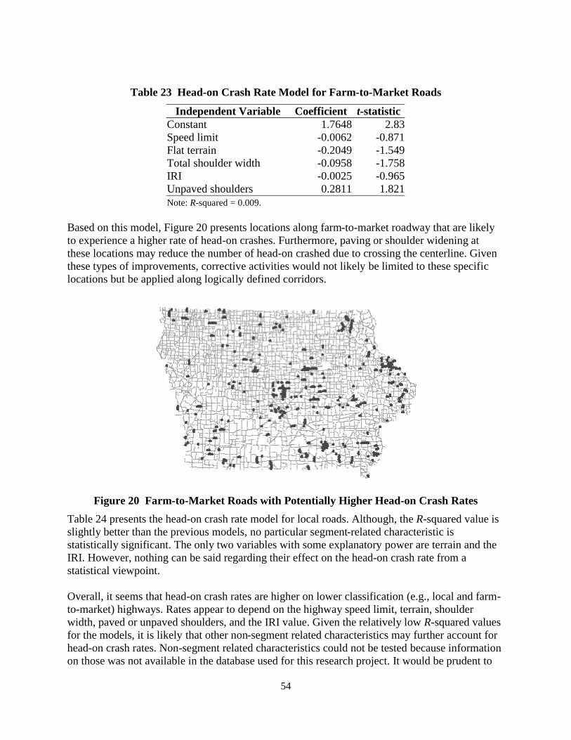
54

Table 23 Head-on Crash Rate Model for Farm-to-Market Roads

Independent Variable Coefficient t-statisticConstant 1.7648 2.83Speed limit -0.0062 -0.871Flat terrain -0.2049 -1.549Total shoulder width -0.0958 -1.758IRI -0.0025 -0.965Unpaved shoulders 0.2811 1.821Note: R-squared = 0.009.

Based on this model, Figure 20 presents locations along farm-to-market roadway that are likelyto experience a higher rate of head-on crashes. Furthermore, paving or shoulder widening atthese locations may reduce the number of head-on crashed due to crossing the centerline. Giventhese types of improvements, corrective activities would not likely be limited to these specificlocations but be applied along logically defined corridors.

Figure 20 Farm-to-Market Roads with Potentially Higher Head-on Crash Rates

Table 24 presents the head-on crash rate model for local roads. Although, the R-squared value isslightly better than the previous models, no particular segment-related characteristic isstatistically significant. The only two variables with some explanatory power are terrain and theIRI. However, nothing can be said regarding their effect on the head-on crash rate from astatistical viewpoint.

Overall, it seems that head-on crash rates are higher on lower classification (e.g., local and farm-to-market) highways. Rates appear to depend on the highway speed limit, terrain, shoulderwidth, paved or unpaved shoulders, and the IRI value. Given the relatively low R-squared valuesfor the models, it is likely that other non-segment related characteristics may further account forhead-on crash rates. Non-segment related characteristics could not be tested because informationon those was not available in the database used for this research project. It would be prudent to

55

extend this research and take into account facility age and /or non-segment related characteristicsto isolate factors responsible for high crash rates.

Table 24 Head-on Crash Rate Model for Local Roads

Independent Variable Coefficient t-statisticConstant -9.4469 -0.385Speed limit 0.1332 0.458Flat terrain 15.8273 1.594Total shoulder width 3.0457 0.846IRI 0.1031 1.5863Unpaved shoulders 3.9293 0.326Note: R-squared = 0.103.


A total of 44,244 GIMS sections were appropriate for analysis of fixed-object crashes. Of these,the majority belonged to local roads followed by farm-to-market roads (see Table 25). Relativelyfew segments belonged to the Interstate highway system. The average fixed-object crash rate was6.7 crashes per MVM. As in the case of head-on crashes, the fixed-object crash rate on localroads was the highest followed by farm-to-market roads. The lowest crash rate was on UShighways followed by the Interstate highways. The least AADT was on farm-to-market roadsfollowed by AADT on local roads. AADT was highest on Interstate highways. The meansegment length was 0.82 km.

Table 25 Segment Characteristics for Fixed-Object Crashes

Type ofSystem

Number ofSegments

Mean CrashRate (MVM)

Crash RateStd. Dev.

MeanAADT(veh)

MeanSegment

Length (m)Interstate 1518 0.946 3.345 24231 518US Hwy 5049 0.729 3.808 7507 600IA Hwy 5427 1.047 6.356 3939 735Farm to Mkt 11534 4.027 18.740 636 1148Local 20716 11.561 41.889 1801 741All 44244 6.707 30.694 3108 823

Results of statistical testing by means of Tukey’s t-tests on differences in mean fixed-objectcrash rates across different types of highways are presented in Table 26. The results indicate thatthe crash rate on US highways was significantly lower than the rate on Interstate highways.However, there was not enough difference in the crash rate between Interstate and Iowahighways. Tests indicated that there were significant differences in fixed-object crash ratesamong the other types of highways.

Fixed-object crash rate models are presented in Tables 27–31. Table 27 shows the model forInterstate highways with an R-squared value of 0.245. The model indicates that Interstatehighway segments in flat and rolling terrain tend to have higher crash rates compared tosegments in hilly terrain. Similarly, segments with asphalt cement concrete (ACC) pavement

56

surface tend to experience higher crash rates compared to other types of surfaces. Segments withpaved shoulders have lower fixed-object crash rates, where as segments with no median barriertend to have higher fixed-object crash rates.

Table 26 Differences in Fixed-Object Crash Rate Means (t-statistic)

Type of System Interstate US Hwy IA Hwy Farm toMkt

Local

Interstate — -0.216(-2.142)

0.1009(0.829)

3.081(15.842)

10.615(34.982)

US Hwy — — 0.317(3.076)

3.177(3.128)

10.831(36.603)

IA Hwy — — — 2.980(15.309)

2.980(15.309)

Farm to Mkt — — — — 7.534(22.202)

Local — — — — —

Table 27 Fixed-Object Crash Rate Model for Interstate Highways

Independent Variable Coefficient t-statistic(Constant) 1.3607 4.541Flat terrain 0.8505 4.845ACC pavement 0.3086 2.014Paved shoulders -2.0060 -7.087Rolling terrain 1.2003 5.650No barrier 3.2231 14.519Note: R-squared = 0.245.

Table 28 presents the fixed-object crash rate model for US highways. The model has a relativelylow R-squared value, indicating that there may be other independent variables (possibly non-segment related) that may account for fixed-object crash rates. The only two significant variablesin the model (at the 90 percent confidence level) are the presence of no barrier and surface width.The absence of median barriers tends to increase fixed-object crash rates. The negative estimatedcoefficient of surface width indicates that fixed-object crash rates tend to be lower on wider UShighways, as expected.

Table 28 Fixed-Object Crash Rate Model for US Highways

Independent Variable Coefficient t-statisticConstant 0.8405 4.536Paved shoulders 0.2474 1.057No barrier 0.2357 1.872Surface width -0.0346 -1.918Note: R-squared = 0.001.

57

Based on this model, Figure 21 presents locations along US Highways that are likely toexperience a higher rate of fixed-object crashes. This, of course, does not take into considerationthe actual number and location of fixed-objects at these locations.

Figure 21 US Highways with Potentially Higher Fixed-Object Crash Rates

Fixed-object crash rate model for Iowa highways is presented in Table 29. Again, the R-squaredvalue is rather low. Two independent variables in the model are statistically significant.Segments in flat terrain tend to have lower fixed-object crash rates while highways withcombination pavement appear to have higher fixed-object crash rates.

Table 29 Fixed-Object Crash Rate Model for Iowa Highways

Independent Variable Coefficient t-statisticConstant 0.7070 2.368No barrier 0.3900 1.262Flat terrain -0.3206 -1.706Combination pavement 1.1698 3.436Note: R-squared = 0.003.

The model for farm-to-market roads (see Table 30) shows that segments with ACC and portlandcement concrete (PCC) pavements tend to have lower fixed-object crash rates, while segmentswith earthen shoulders tend to have higher fixed-object crash rates. The statistical significancefor the latter variable is at the 90 percent level.

Finally, the model for fixed-object crash rate on local roads has a low R-squared value (see Table31). Nonetheless, the model indicates that several independent variables as statisticallysignificant in explaining fixed-object crash rates. Local road segments in flat terrain tend to havehigher fixed-object crash rates, while ACC and PCC segments tend to have lower rates.Similarly, segments with greater number of lanes (a proxy for surface width) tend to have lowerfixed-object crash rates. Higher speed limits on local roads tend to result in higher fixed-object

58

crash rates. Segments with earthen shoulders tend to have higher fixed-object crash rates thoughthe variable is statistically not significant.

Table 30 Fixed-Object Crash Rate Model for Farm-to-Market Roads

Independent Variable Coefficient t-statisticConstant 6.7805 2.746Speed limit 0.0162 0.581ACC pavement -6.9317 -17.462PCC pavement -6.5437 -13.435Shoulder type (earth or gravel) 0.6165 1.723Note: R-squared = 0.029.

Table 31 Fixed-Object Crash Rate Model for Local Roads

Independent Variable Coefficient t-statisticConstant 17.1885 8.155Flat terrain 1.8017 1.943ACC pavement -10.6321 -9.251PCC pavement -11.1118 -9.159Number of lanes -1.9274 -3.768Speed limit 0.0613 2.591Shoulder type (earth or gravel) 0.8622 1.324Note: R-squared = 0.031.

Overall, data analysis indicated that fixed-object crash rates tend to be higher on lowerclassification (local and farm-to-market) highways. It appears that terrain, type of pavement,paved or unpaved shoulders, the absence of median barriers, surface width, and number of lanestend to affect fixed-object crash rates on different types of highways. The models had rather lowR-squared values, indicating the possibility that facility age and/or other non-segmentalcharacteristics may further explain fixed-object crash rates.


The model developed to examine the impact of the curve length and degree of curvature oncrashes is presented in Table 32. Despite the low R-squared value, the model shows strongrelationships between the curve length and degree of curvature and horizontal curve crash rates.

The model shows that the degree of curvature has a direct impact on crash rate increments onhorizontal curves. That is, the crash rate significantly increased with increased degree ofcurvature. Furthermore, the model indicates that the crash rate on shorter curve lengths issignificantly higher than the crash rate on longer curves. This is probably because sharp curvesare usually shorter than mild curves (33).

59

Table 32 Horizontal Curve Crash Rate Model

Independent Variable Coefficient t-statistic(Constant) 1.5604 12.77Degree of curvature 0.0649 3.99Curve length -0.0004 -3.89Note: R-squared = 0.0134.

61

5 CONCLUSIONS AND RECOMMENDATIONS

In Iowa, as in most states, highway engineering safety improvement programs are reactive. Inother words, safety countermeasures are applied to the roadway only after high crash rates havebeen observed. The objective of this project was to quantify the impact of highway geometry anddesign features on crash rates, enabling agencies to proactively identify and mitigate futureproblem areas.

The application of GIS in this project has enabled the research team to identify and analyzeroadway segments characterized by specific criteria that are not identified by conventional crashanalysis. Along the way, methods were developed for solving intermediate problems that willalso find utility at state DOTs (e.g., determining most recent daily entering vehicles atintersections and reviewing and defining extents or location specific analysis). Another usefulproduct is an improved corridor analysis methodology.

The project produced the following items:

• curve database for Iowa, with radii and length attributes• procedures for identifying high crash locations of five types• statistical models of the relationship between geometric features and crash rates• candidate lists (maps and tables) for improvement (Iowa top 30 lists) for five problem

types

63

ACKNOWLEDGMENTS

The research team would like to thank the Iowa Department of Transportation and the IowaHighway Research Board for support of this research.

65

REFERENCES

1. Iowa Safety Management System. Iowa Strategic Highway Safety Plan. Draft. IowaDepartment of Transportation, Ames, Iowa, Aug. 1999.

2. Strategic Plan for Fiscal Years 1997–2002. U.S. Department of Transportation.http://www.dot.gov/hot/dotplan.html.

3. Shaw-Pin, M., and H. Lum. Statistical Evaluation of the Effects of Highway GeometricDesign on Truck Accident Involvements. Transportation Research Record 1407,Transportation Research Board, National Research Council, Washington, D.C., 1993, pp.11–23.

4. Zegger, C. V., J. R. Stewart, F. M. Council, D. W. Reinfurt, and E. Hamilton. Safety Effectsof Geometric Improvements on Horizontal Curves. Transportation Research Record 1356,Transportation Research Board, National Research Council, Washington, D.C., 1992, pp.11–19.

5. Luediger L., E. M. Choueiri, J. C. Hayward, and A. Paluri. Possible Design Procedure toPromote Design Consistency in Highway Geometric Design on Two-Lane Rural Roads.Transportation Research Record 1195, Transportation Research Board, National ResearchCouncil, Washington, D.C., 1988, pp. 111–122.

6. Feng-Bor, L. Flattening of Horizontal Curves on Rural Two-Lane Highways. Journal ofTransportation Engineering, Vol. 116, No.2, March/April 1990, pp. 181–193.

7. Al-Masaeid, H. R., M. Hamed, M. About-Ela, and A. G. Channam. Consistency ofHorizontal Alignment for Different Vehicle Classes. Transportation Research Record1500, Transportation Research Board, National Research Council, Washington, D.C., 1995,pp. 178–183.

8. Anderson, I. B., K. M. Bauer, D. W. Harwood, and K. Fitzpatrick. Relationship of Safety ofGeometric Design Consistency Measures for Rural Two-Lane Highways. TransportationResearch Board 78th Annual Meeting, National Research Council, Washington, D.C.,1999.

9. Fink, K. L., and R. A. Krammes. Tangent Length and Sight Distance Effects on AccidentRates at Horizontal Curves on Rural Two-Lane Highways. Transportation ResearchRecord 1500, Transportation Research Board, National Research Council, Washington,D.C., 1995, pp. 162–168.

10. Matthews, L. R., and J. W. Barnes. Relation Between Road Environment and CurveAccidents. Proceedings of the 14th ARRB Conference, Part 4, pp. 105–120.

11. Tom, G. K. J. Accidents on Spiral Transition Curves. ITE Journal, September 1995, pp.49–53.

66

12. Council, F. M., Safety Benefits of Spiral Transitions on Horizontal Curves on Two-LaneRural Roads. Transportation Research Record 1635, Transportation Research Board,National Research Council, Washington, D.C., 1998, pp. 10–17.

13. Budhu, G. A Five-Step Approach to the Incorporation of Fixed Object Crashes in theEconomic Analysis and Prioritization of Highway Projects—Case Study of Louisiana.Traffic Congestion and Traffic Safety in the 21st Century—Challenges, Innovations, andOpportunities, ed. R. F. Benekohal. ASCE, New York, 1997.

14. Lawson, S. D. Single-Vehicle Collisions with Roadside Objects: The Problem and Its Needof Treatment. Traffic Engineering & Control, Vol. 26, No. 10, Oct. 1985, pp. 489–494.

15. Mak, K. K. Safety Effects of Roadway Design Decisions—Roadside. TransportationResearch Record 1512, Transportation Research Board, National Research Council,Washington, D.C., 1995, pp. 16–21.

16. Zegger, C. V., et al. Cost-Effective Geometric Improvements for Safety Upgrading ofHorizontal Curves. Report FHWA-RD-90-021. FHWA, U.S. Department ofTransportation, Washington, D.C., 1991.

17. Jones, I. S., and S. Baum. Analysis of the Problem of Urban Utility-Pole Accidents.Transportation Research Record 681, Transportation Research Board, National ResearchCouncil, Washington, D.C., 1978, pp. 89–92.

18. Daniel, S. T., and T. Barnett. Case Study: Poles in the Urban Clear Zone. TransportationResearch Record 1233, Transportation Research Board, National Research Council,Washington, D.C., 1989, pp. 155–163.

19. Mintsis, G., and M. Pitsiava-Latinopoulou. Traffic Accidents with Fixed RoadsideObstacles: A Study of the Greek Rural Road Network. Traffic Engineering & Control. Vol.31, No. 5. May 1990, pp. 306–311.

20. Turner, D. S., E. R. Mansfield. Urban Trees and Roadside Safety. Journal ofTransportation Engineering, Vol. 116, No. 1. Feb. 1990, pp. 90–104.

21. Zegeer, C. V., and F. M. Council. Safety Relationships Associated with Cross-SectionalRoadway Elements. Transportation Research Record 1512, Transportation ResearchBoard, National Research Council, Washington, D.C., 1995, pp. 29–36.

22. Barbaresso, J. C., and B. O. Bair. Accident Implications of Shoulder Width on Two-LaneRoadways. Transportation Research Record 923, Transportation Research Board, NationalResearch Council, Washington, D.C., 1983, pp. 90–97.

23. Injury Facts. National Safety Council, Itasca, NY, 1999.

67

24. Al-Senan, S, H., and P. H. Wright. Prediction of Head-on Accident Sites. TransportationResearch Record 1122, Transportation Research Board, National Research Council,Washington, D.C., 1987, pp. 79–85.

25. Zegeer, C. H., R. C. Deen, and J. G. Mayes. Effect of Lane and Shoulder Widths onAccident Reduction on Rural Two-Lane Roads. Transportation Research Record 806,Transportation Research Board, National Research Council, Washington, D.C., 1981, pp.33–43.

26. Knuiman, M. W., F. M. Council, and D. W. Reinfurt. Association of Median Width andHighway Accident Rates. Transportation Research Record 1401, Transportation ResearchBoard, National Research Council, Washington, D.C., 1993, pp. 70–82.

27. Clissold, C. M. Wet Weather Injury Accidents on New Zealand Roads. TransportationResearch Record 624, Transportation Research Board, National Research Council,Washington, D.C., 1976, pp. 136–139.

28. Turner, D. S., D. B. Fambro, and R. O. Rogness. Effects of Paved Shoulders on AccidentRates for Rural Texas highways. Transportation Research Record 819, TransportationResearch Board, National Research Council, Washington, D.C., 1981, pp. 30–37.

29. Daubert, D. B. Stop Versus Yield Signs on Low-Volume Rural Roads. Proceedings 6 ofSixth International Conference on Low-Volume Roads, Vol. 1. Minneapolis, June 1995, pp.30–37.

30. Walker, F. W., and S. E. Roberts. Influence of Lighting on Accident Frequency at HighwayIntersections. Transportation Research Record 562, Transportation Research Board,National Research Council, Washington, D.C., 1976, pp. 73–78.

31. Hanna, J. T., T. E. Flynn, and W. L Tyler. Characteristics of Intersection Accidents in RuralMunicipalities. Transportation Research Record 601, Transportation Research Board,National Research Council, Washington, D.C., 1976, pp. 79–82.

32. Pant, P. D., Y. Park, S. V. Neti, and A. B. Hossain. Comparative Study of Rural Stop-Controlled and Beacon-Controlled Intersections. Transportation Research Record 1692,Transportation Research Board, National Research Council, Washington, D.C., 1999, pp.164–172.

33. Reinfurt D. W., C. V. Zeeger, B. J. Shelton, and T. R. Neuman, Analysis of VehicleOperations on Horizontal Curves. Transportation Research Record 1318, TransportationResearch Board, National Research Council, Washington, D.C., 1991, pp. 43–50.

Appendix AIowa DOT High Crash Location Ranking Procedure

A-1

The Iowa DOT generates an annual list of top 100 high crash locations using a five-year periodstatewide crash data (The latest ranking uses the 1994–1998 crash data). The crash locationsconsist of nodes and links. The following roadway facilities have been classified as nodes:

• intersections• ramp terminals• railroad crossings• grade separation structures• bridges• road ends• 90 degree turns (when each leg is at least quarter mile long)• county lines• major signalized commercial entrances

Links are the distances between adjacent nodes. Crashes assigned to a link do not include thecrashes assigned to either of the two nodes.

To become an initial candidate location, a site needs to meet one of the following three criteria:one fatal crash, four injury crashes, or a total of eight crashes. Once the candidate locations havebeen determined, a three-phased ranking scheme is used as the basis to determine the high crashlocations (see flow diagram, Figure 1).

Figure 1 Current Approach to Identify High Crash Locations in Iowa

1 Crash Frequency

The first ranking is based on the number of crashes, or frequency, occurring at each location.Each site is given a ranking based on the number of crashes. A site that has the highest frequencyof crashes receives the number one ranking. In the case of a tie, each location receives the samerank and the subsequent ranking is skipped.

A-2

2 Crash Rate

Second, each site is ranked according to the crash rate. For nodes and links up to 0.6 miles, thecrash rate is calculated using the following equation:

where

MEV is million entering vehicles, andDEV is daily entering vehicles for nodes or average daily traffic (ADT) for links.

For links 0.6 miles or longer, the DEV is determined using the following equation:

The site that has the largest crash rate receives the top ranking. The same implication of a tieapplies to this ranking as well. For locations where their traffic volumes are unknown the rankingof zero is assigned.

3 Crash Loss

Finally, each site is ranked according to the financial loss from the crashes. This is determined byusing values based on the injuries sustained in each crash type as seen in Table 1. These valuesare then multiplied by the number of people that fall into each category. For example, if twofatalities, four major injuries, 12 minor injuries, and 15 possible injuries occur at a location, thevalue loss due to injuries is $2,206,000 (2 × $800,000 + 4 × $120,000 + 12 × $8,000 + 15 ×$2,000).

Table 1 Crash Costs by Injury Type

Type Dollar ValueFatal $800,000Major Injury $120,000Minor Injury $8,000Possible Injury $2,000

Property damage is incorporated as well. Officers report estimates on the crash report form. Insome instances there is no estimate of property damage; when this occurs a default value of

days/year5365

1000000

DEV

CrashesofNumberRate/MEVCrash

××=

DEV3.0

LengthLinkABSDEV ×

=

A-3

$2,000 is used. All of these values are summed up and result in a ranking based on the value lostat each location.

To determine the top 100 high crash locations within the state, each of the three ranks are addedtogether and a final ranking is performed with the lowest cumulative ranking receiving thehighest ranking of a 1. Those falling within the top 100 ranking are deemed high crash locationswithin Iowa. An example of this process is shown in Table 2, using fictitious data, for the top 13locations throughout the state. This process is performed for approximately 17,000 locations thatmeet the initial threshold.

Table 2 Example of High Crash Location Ranking Process

ReferenceNode

# ofCrashes

Rank CrashRate

Rank DollarLoss

Rank Total Rank StatewideRank

11111111 47 5 2.63 23 2,327,237 15 5+23+15 = 43 133333333 29 31 Unknown 0 1,909,420 20 31+0+20 = 57 244444444 25 35 2.76 15 2,734,603 9 35+15+9 = 59 322222222 24 37 2.71 19 3,150,760 4 37+19+4 = 60 455555555 53 1 2.46 29 1,373,300 35 1+29+35 = 65 577777777 40 10 2.92 8 1,120,949 47 10+8+47 = 65 500000000 34 21 2.40 33 2,000,850 18 21+33+18= 72 710101010 49 2 2.65 21 1,117,965 50 2+21+50 = 73 832323232 28 32 2.41 32 2,684,259 10 32+32+10= 74 988888888 19 51 3.15 3 1,824,587 22 51+3+22 = 76 1099999999 18 53 2.47 28 3,501,985 1 53+28+1 = 82 1166666666 36 18 2.28 41 1,740,548 27 18+41+27= 86 1221212121 32 24 1.98 61 1,357,951 39 26+61+39 =124 13

As indicated, crash frequency, rate, and cost equally contribute in ranking of the top 100 highcrash locations. It was also noted that in current ranking procedure roadway links are treated asnodes. A link length of less of 0.6 miles is not taken into the consideration in the crash ratecalculation. It is only for the longer link (0.6 miles or greater) where the link length is employedin a form of a multiplier (Link Length / 0.3), rather than the actual link length, in the crash rateequation.

Appendix BHorizontal Curve Identification Strategies

B-1

1 Glossary

Quantitative Assessment - Accuracy level of the method – one minus type I error plus type IIerrorType I Error - H1 is selected as being correct when H0 is correctType II Error - H0 is selected as being correct when H1 is correct• H0: not a curve• H1: a curve

Through the visual inspection of the sites’ maps in the GIS environment, each record ismarked as being a curve or a line. The discrepancies between the two procedures definethe two error types.Type I error is the percent of records that have been tagged as curves, but the visualinspections indicate differently.Type II error (i.e., a more serious error) is the percent of records that have been tagged asnot curves, but the visual inspections indicate differently.

Fixed Cost - Training and development costMarginal Cost - Changes in cost for an additional site studyQualitative Assessment - What are the implications if we make mistakes

B-2

2 Curve Identification Procedures Overview

2.1 Preliminary Technique I - County TestedIn its first version, the curve identification technique determined the best combination ofstrategies as well as appropriate threshold values for the string's "weighed-difference" (see thedescription of Length (string) strategy in Appendix B), deflection angle, and segment lengththrough a trail-and-error analysis. For example, using the following logical statement, thecurves' segments were identified. Figure 1 shows the identified segments in Story County, Iowa.

((([Dfbearing]>5) and ([Flegs]=2) and([Dfbearing]<>999)) or(([Dtbearing]>5) and ([Tlegs]=2) and([Dtbearing]<>999)) or(([Dfbearing]>5) and ([Dfbearing]<80)) or(([Dtbearing]>5) and ([Dtbearing]<80)) or(([Dfbearing]>80) and ([Flegs]=2) and([Dfbearing]<>999)) or(([Dtbearing]>80) and ([Tlegs]=2) and([Dtbearing]<>999)) or(( [Sdiffer] < -3) and ([Length] < 400 ))) and([Func]<50)

Figure 1 Identified Curves' Segments Using

{B-2 OR [L (st) AND L (seg)]}

B-3

Once the lines' segments filtered out, the identified curves' segments were visually inspected.The visual curve identification process relies primarily on three data sets: aerial photography,roadway cartography (with associated roadway characteristics), and Roadware driven lanecenterline data. The latter two provide the components necessary to calculate curvecharacteristics, e.g. length, radius, and degree. Everywhere, aerial photography provides the bestrepresentation of roadway alignment, allowing the user to better identify curve extents on thecartographic and Roadware representations of the roadway. An analyst could also manuallymeasure pertinent curve characteristics from these images, but this would be a labor-intensiveprocess.

In Iowa, Roadware data provides the next best representation of roadway alignment. As part ofthe Iowa Pavement Management Program (IPMP), Roadware uses a differential GPS equippedvehicle to collect pavement condition data along a portion of Iowa's highway network. Thesedata are summarized to 100-meter segments of roadway and, when plotted, provide a relatively"smooth" representation of the roadway as driven (accurate to within approximately five meters).Roadware data, however, are not available for all roadways and may not be continuous due toloss of signal or data reduction errors.

The last data set, cartography, is available statewide for all roadways. Important roadwaycharacteristics, such as traffic, are also associated with these data. Roadway alignment andchanges in alignment (including curves) are represented by a series of variable length linesegments. Therefore, curve extents can be difficult to identify from this data set alone. Theaccuracy of these data range from approximately 12 to 50 meters.

In general, aerial photography and Roadware lane centerline data provide the bestrepresentations of actual roadway alignments, facilitating more accurate curve identification.Moreover, Roadware data will likely yield more accurate curve measurements. However, thesedata are not available for all roadways and do not possess essential roadway characteristics.Cartography serves as a comprehensive data set, fulfilling all necessary data requirements.

Next, the following steps were conducted to calculate curve radii and degree of curvature:

• Eliminate the mistakenly selected tangent segments through visual inspections• Manually put boxes around curves• Perform clipping

• Assign a unique number to each polygon• Assign the polygon unique numbers to the curves• Calculate the length of curve• Calculate weighted AADT

• Combine the clipped segments• Calculate chord and curve lengths• Calculate the curve radii and degrees of curvature

The first two steps are performed manually. In the first step, all selected segments wereinspected for possible errors. The mistakenly selected segments were eliminated and polygonswere placed around remaining curves using the procedure described in Appendix C.

B-4

Finally, a closed form solution was used to calculate the curves' radii and degrees. Usingcircular curve equations (Equations 1 and 2), Equation 3 is derived to define the relationshipbetween the length and chord length of the curves. Equation 3 is a function of θ (i.e., half of thedeflection); thus, it can be rearranged into Equation 4. Equation 4 and its derivative (Equation 5)are then plugged into the Newton iteration equation (Equation 6) to estimate θ. This, in turn,facilitates the calculation of the radius and degree of a curve ( R and D) through the use ofEquations 1 and 7, respectively.

θRL 2= (1)

xyztrianglesee;sin2

θRC = (2)

θθsin=

L

C(3)

( )L

Cf

n

nn −=

θθ

θsin

(4)

( )n

n

n

nnf

2

sincos

θθ

θθ

θ −=′ (5)

( )( ) 2,...1,,0n;1 =′

−=+n

nnn f

f

θθ

θθ (6)

RD

579.5729= (7)

y

x

z

R

C

L

θ

B-5

whereL = Curve lengthC = Chord lengthR = Curve radiusD = Curve degree

angleDeflection;2

=∆∆=θ

As shown in the table below, the values of θ''s converge rather rapidly.

C (ft) L (ft) Theta (0) Theta (1) Theta (2) Theta (3) Theta (4) Theta (5) Theta (6) R (ft) D (deg)949 963 1 0.52189 0.343226 0.29917 0.296007 0.29599 0.29599 1626.74 3.52943 961 1 0.53581 0.371941 0.33786 0.336188 0.33618 0.33618 1429.28 4.01416 427 1 0.55916 0.417759 0.3953 0.394685 0.39468 0.39468 540.94 10.59780 790 1 0.51565 0.329986 0.28043 0.276148 0.27611 0.27611 1430.56 4.01774 788 1 0.53261 0.365435 0.32931 0.327377 0.32737 0.32737 1203.53 4.76

2.2 Preliminary Technique II - Statewide TestedDue to limited time and resources, statewide curve identification was confined to potential"problem" curves or consecutive curves. In this technique, only primary road crashes reportedby the officer in the field as occurring on a curve were selected.1 After visually inspectingidentified sites, polygons were placed around isolated curves, consecutive curves, and theirinfluence areas. Figure 2 shows a polygon around an isolated curve. Curves were defined byestimating the locations of their point of curvature (PC) and point of tangency (PT). Curveinfluence areas were defined as extending approximately 200 meters longitudinally, along theadjacent tangents, from these points.2 If the influence area of consecutive curves overlaps, thecurves were included in a single polygon.

The remaining steps, beginning with "perform clipping", are essentially the same as the stepsdefined in version 1. Because of the aforementioned curve selection criteria (i.e., selecting onlythe potential "problem" curves), calculations of the curves' characteristics (i.e., chord and curvelengths, radius, and degree) were not applicable to this technique. The detail procedure ispresented in Appendix C.

1 The Iowa DOT will no longer maintain the [Road_geome] field in the A Crash Records. The [Road_geome] fieldcontains crash site geometric information reported by the on site officer. The final report will provide an alternativestrategy (or strategies) for future initial identification of curves.2 L. Reudiger, B. Psarianos, and T. Mailaender. Highway Design and Traffic Safety Engineering Handbook,McGraw Hill, NY, 1999, Table 12.2.

B-6

Figure 2 Example: A Polygon Drawn Around an Isolated Curve

2.3 Enhanced Technique I - County TestedTo improve the quality of the curves' characteristics, the analysis was limited to primary andsecondary paved roadways throughout a county (e.g., Story county). These roadways wereselected using Iowa DOT roadway centerline cartography (with associated base recordsattributes) and visually inspected to identify horizontal curve locations. Aerial photographs wereused in conjunction with the roadway cartography to provide a more accurate representation ofroadway alignment.

Upon identifying a possible curve location, lines of tangency were temporarily drawn along theroadway alignment presented by the aerial photographs. Curves were then defined by manuallydigitizing a line string (polyline) beginning and terminating at the approximate points oftangency. These digitized curves should provide better overall curve lengths and chord distancesthan when using cartography alone.

Next, a polygon was placed around the newly digitized curve and an adjacent portion of existingroadway cartography of the same approximate length and alignment. All attributed crashes werealso included within the polygon extents. A unique identifier was assigned to each polygon, andthe curves contained within each polygon. (Curves within the same polygon shared the samecurve identifier.) The curve polygons were then used to clip and extract roadway attributes fromcartography and assign these data, included weighted traffic values, to the digitized curves.Crash data were also summarized based on the unique curve identifier and assigned to thedigitized curves. Digitized curve chord distance and length were calculated within GIS. Usingthese values, the closed form solution (presented in Equations 1 through 7) calculated curveradius and degree of curvature.

B-7

3 Detailed Curve Identification Procedures

3.1 On-curve Crashes (String-based)3.1.1 DefinitionA string is tagged as a curve when at least 50 percent of its associated accident records aredesignated as “on-curve” accidents.

3.1.2 Cost

Manpower (days)Ali Zach Student Amount ($)

Fix cost 10 5 2Marginal cost 1 1 4

3.1.3 Qualitative AssessmentThis strategy may result in over estimation of horizontal curves’ crash rates.

• All accidents on a designated curve are considered as “on-curve” even though only 50percent of those were actually reported as on-curve accidents.

• An entire length of a designated string is considered as the curve length when only asection of the string is actually curved.

3.1.4 Procedure• Open a new View• Click on Add Theme icon• Select road and accident shape files

Spatial join the road and accident attributes tables• Highlight road theme by clicking on its text in the View• Click on Open Theme Table to open road attributes table• Highlight accident theme by clicking on its text in the View• Click on Open Theme Table to open accident attributes table• Click on [Shape] field of the road attributes table• Click on [Shape] field of the accident attributes table• Click on Join icon

The road attribute table closes. The new accident attributes table now includes all relatedroadway geometric data for each accident record.

Count the total number of accidents on each string• Click on the new accident attributes table to make it active• Click on Query Builder icon• Input the following expression in the dialog box

[Distance] < 6.769

• Click on [Road_link] field of the new accidents attributes table• Click on Field Menu/Summarize

B-8

• Click OK to save the new table (sum1.dbf)• Rename the [Count] field to [all_count] using Table/Properties/Alias Menu

Count the on-curve accidents on each string• Click on the new accident attributes table to make it active• Click on Query Builder icon• Input the following expression in the dialog box

[Road_geometry] = 4 or [Road_geometry] = 5 or [Road_geometry] = 6and [Int_class] = 0 and [Distance] < 6.769

• Click on [Road_link] field of the new accidents attributes table• Click on Field Menu/Summarize• Click OK to save the new table (sum2.dbf)• Rename the [Count] field to [curve_count] using Table/Properties/Alias Menu

Calculate percent of on-curve accidents for each string• Click on [Road_link] field of the sum1.dbf table• Click on [Road_link] field of the sum2.dbf table• Click on Join icon

The sum1.dbf table closes. The sum2.dbf table now has both the [all_count] and [curve_count]field

• Click Table Menu/Start Editing• Click Edit Menu/Add field• Name the new field [%on-curve]• Select the [%on-curve] field and click on Calculate icon• Enter the following expression

By performing a query and equating the [%on-curve] field equal or greater than 0.50, theselected strings will be designated as “curves.”

3.1.5 Illustration

]_[

]_[]_[1

countall

countcurvecountall −−

B-9

3.2 On-Curve Crashes (Segment-based)3.2.1 DefinitionA string consists of a number of segments. A segment is tagged as a curve when at least 50percent of its associated accident records are designated as “on-curve” accidents. By examiningthe status of the segments prior and after the marked segment with respect to their on-curveaccident percentages, this strategy could lead to determination of the beginning and end of acurve.

3.2.2 Cost



3.2.3 Qualitative AssessmentThis strategy requires an extensive data manipulation.

3.2.4 ProcedureThe road segment shape file has a unique 15-digit identifier field [Index] consists of thesegments’ county, jurisdiction, etc. identification numbers. These identification numbers, on theother hand, are listed under separate fields in the road string shape file. To make these two filescomparable a similar unique identifier field has to be created by concatenating the county,jurisdiction, etc. fields in the road string file. These new identifiers of the strings consist of 14digits. Furthermore, the identifiers in the road segment file should also be modified, in whichtheir sixth digits will be eliminated.

• Open a new View• Click on Add Theme icon• Select road shape file• Highlight road theme by clicking on its text in the View• Click on Open Theme Table icon

Add a new field in the road attributes table for the new 14-digit identifiers• Click on Open Theme Table icon• Click on Table/Start editing Menu• Click on Edit/Add Field Menu• Name the new field New_Index• Select String for the field type• Close the add-field window• Select the [New_Index] field and click on Calculate icon• Enter the following expression to create a 14-digit identifier for each record

[Co].Asstring + [Jurisd].Asstring + [Sys].Asstring + [Stat].Asstring +

B-10

[Pre].Asstring + [Route].Asstring + [Seq].Asstring

• Click on Table/End editing Menu

Next, the sixth digits of the identifiers in the road segment shape file [Index] are eliminated.• Click Add Theme icon• Select segment shape file• Highlight segment theme by clicking on its text in the View• Click on Open Theme Table icon

Add a new field in the road segment attribute table for the new 14-digit index• Click on Open Theme Table icon• Click on Table/Start editing Menu• Click on Edit/Add Field Menu• Name the new field New_Index• Select String for the field type• Close the add-field window• Select the [New_Index] field and click on Calculate icon• Enter the following expression to create a 14-digit identifier for each record

[Index].left(5) + [Index].right(9)

• Click on Table/End editing Menu

Now both road string and road segment shape files include [New_Index] fields, which containunique 14-digit identifiers. To determine whether or not a segment is a curve, it is assumed thatif at least 50 percent of total number of accidents assigned the segment are on-curve accidents,the segment is then marked as a curve segment.

Spatial join the segment and accident attributes tables• Click Add Theme icon• Select accident shape file• Highlight accident theme by clicking on its text in the View• Click on Open Theme Table icon• Click on [Shape] field of the segment attributes table• Click on [Shape] field of the accident attributes table• Click on Join icon

The segment attributes table closes. The new accident attributes table contains all relatedsegment data for each accident record. Next, road string information will be added to the all-accident data.

Join the road and all-accident attribute tables• Click on [New_Index] field of the road table• Click on [New_Index] field of the accident table• Click on Join icon

B-11

The road attributes table closes. The new accident attributes table contains all related road aswell as segment data for each accident record.

Select the accident records that are close to roadways. The majority of the records are within 0to 0.007 range.

• Click on Query Builder icon• Input the following expression in the dialog box

[Distance] < 6.769

• Click on Theme Menu/Convert to Shapefile to create a new theme for the accidentattributes table under all-acc-seg name

Select curve accidents, which are not occurred at intersections• Highlight all-acc-seg theme by clicking on its text in the View• Click on Query Builder icon

• Enter the following expression in the dialog box

[Road_geometry] = 4 or [Road_geometry] = 5 or [Road_geometry] = 6and [Int_class] = 0

Count the on-curve accidents on each segment• While the on-curve accident records are highlighted in the active all-acc-seg attributes

table, click on Menu/Xtools/Table Frequency• Select [Seg_seq] and [Index] fields from the Select Frequency Field(s) dialog box and

click OK• Click OK in the Select Summary Field(s) dialog box without making any selection• Save the new table as brsegsum_curv• Rename the [Frequency] field to [curve_count] using Table/Properties/Alias Menu

Count the total number of accidents on each segment• Click Select None icon while the all-acc-seg attributes table is active• Click on Menu/Xtools/Table Frequency• Select [Seg_seq] and [Index] fields from the Select Frequency Field(s) dialog box and

click OK• Click OK in the Select Summary Field(s) dialog box without making any selection• Save the new table as brsegsum• Rename the [Frequency] field to [all_count] using Table/Properties/Alias Menu

The reason for renaming the [Frequency] fields is to eliminate errors when calculating curveaccident percentages.

Join brsegsum and brsegsum_curv tables with the co_03_seg shape file. Having both [all_count]and [curve_count] fields in a shape file enables us to calculate curve accident percentages and toshow them on the map.

B-12

A unique identifier field needs to be created for each of these three tables to facilitate joiningprocedures. This field is the combination of [index] and [Seg_seq] fields.

• Click on Table/Start editing Menu• Click on Edit/Add Field Menu• Name the new field [Index_seg]• Select String for the field type• Close the add-field window• Select the [Index_seg] field and click on the Calculate icon• Enter the following expression (“++” symbol combines the two strings with a space

between the two fields)

[Index] ++ [Seg_seq]

• Click on Table/End editing Menu• Join the brsegsum table and co_03_seg shape file by selecting the [Index_seg] fields

when co_03_seg file is active• Join the brsegsum_curv table and co_03-seg shape file by selecting the [Index_seg] fields

when co_03_seg file is activeBoth brsegsum and brsegsum_curv tables close. Now the co_03_seg attributes file includes thetotal as well as on-curve accidents for each segment. Next, the curve accident percentages aredetermined for each segment.

• While the co_03_seg attributes table is open click on Table/Start editing Menu• Click on Edit/Add field Menu• Name the new field [%curve_acc]• Click on Field/Calculate Menu• Enter the following expression

Next, the number of on-curve accidents and on-curve accident percentages are shown on themap.

• Click on Theme Menu/Convert to Shapefile to create a new theme for the co_03_segattributes table under on_curve_seg name

• Add the on_curve_seg theme to a new View• Double click on the on_curve_seg theme in the View to open Legend Editor• Select Graduated Symbols from the Legend Type pull down menu• Select [curve_count] for the Classification Field and click on Apply button

Repeat the above five steps for the on-curve accident percentages• Click on Theme Menu/Convert to Shapefile to create a new theme for the co_03_seg

attributes table under percent_on_curve name• Add the percent_on_curve theme to the new View• Double click on the percent_on_curve theme in the View to open Legend Editor• Select Graduated Symbols from the Legend Type pull down menu

]_[

]_[]_[1

countall

countcurvecountall −−

B-13

• Select [%curve acc] for the Classification Field and click on Apply button

3.2.5 Illustration

B-14

3.3 Bearing-Method I

3.3.1 DefinitionThe deflection angle of each segment with respect to its successive one is calculated using aMicrosoft Excel spreadsheet. A segment is tagged as a curve when its deflection angle is eithergreater or equal than a selected value.

3.3.2 Quantitative Assessment3.3.2.1 Type I Error3.3.2.2 Type II ErrorThe accuracy level of the strategy was determined for the deflection angles of 1 to 15 degrees.As shown in the figure below, a 74 percent accuracy level (i.e., highest level) is observed at the6° deflection angle when the Type I and Type II errors are 8 and 18 percent, respectively.However, if the concern is not to miss a curve when actually is a curve (i.e., Type II error), asegment should be tagged as a curve when its deflection angle is either greater or equal than 1°(or even less than 1° for a lower Type II error).

3.3.3 Cost



3.3.4 Qualitative AssessmentThis strategy requires an extensive data manipulation.

0

10

20

30

40

50

60

70

80

1 3 5 7 9 11 13 15

Angle (degree)

Per

cen

t

Type I Type II Accuracy

B-15

3.3.5 ProcedureProvided an Excel spreadsheet containing segments’ x-y coordinates, the angle that eachsegment makes with its successive segment is calculated. Depending on the orientation of thesegments constituting the network, some of the values may be negative. However, since theprimary concern in this part of the analysis is the calculation of angles between the segments,absolute values of the differences are considered.

It is assumed that any segment with the absolute angle of 5° (or 10° in another case) or greater isconsidered as a curve. The accuracy of this strategy is measured by overlaying the study site’smaps on its aerial photos using GeoMedia.

• Open GeoMedia• Create new Geo workspace• Accept the default file name normal.gwt• In Geo workspace 1, click on "Warehouse" on the Menu bar• Click on New connection• Accept the default Access option for the database type• Accept the default Access Connection 1• Select the site database (e.g., allamakee.mdb)• Open the file as read only or read-write• In Geo workspace 1, click on Analysis on the Menu bar• Click on New Query• Use Select Features in Access Contribution 1 and click on CL_99 (This is the file that

contains the road network data of Allamakee county.)• In Filter, use RTE_INDICATOR=1 (This option will only load the major roads in the

network.)• In Geo workspace 1, click on "Analysis" on the Menu bar• click on Join• For the "left side of join", use Access Contribution 1 and CL_99• For the "right side of join", use Access Contribution 1 and BRCURVE (This the file that

contains the horizontal curves in the road network of Allamakee county.)• For "available attributes" click on [Road link] on both the left side and the right side• For the "type of join" select "right outer"• For the display option check the box for "Map window" and uncheck the box for "Data

window" (This will ensure that the network will be displayed only in the map windowand not in the data window.)

Apply different color and weight to the join of CL_99 and BRCURVE files.• Right click on the CL_99 and BRCURVE join in the legend window

B-16

• Click on Properties• Click on Style and make necessary modifications

Next the aerial photos are inserted. The road network will be overlaid on the aerial photos.• Click on Insert on the Menu bar• Click on Image• Select the site’s aerial photos file (e.g., Allamakee.doq; file type: tiff(*tiff))• In the Geo workspace 1, double click on a link (string) of the road network to open an

attribute table• Identify the [unique identifier] of the string from the attribute table• Based on the this [unique identifier] select the appropriate Excel file of the site study• Close the attribute table and click on the string• Use the Edit Geometry icon to bring up the points which make up the string• With the assistance of the actual road network on the background, visually inspect

whether the points are lying on curves or lines (see Figures 3 and 4)• Adopt the same procedure for all the links in the network

Figure 3 Overlay of Network Maps and aerial photos – Exact Match

43091A 21.TIF

Jo in o f CL_99 and BRCURV E

Query 1

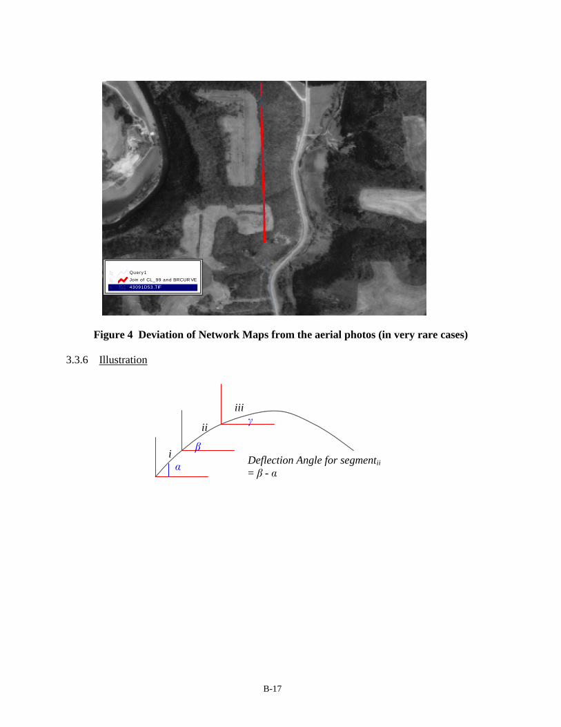
B-17

Figure 4 Deviation of Network Maps from the aerial photos (in very rare cases)

3.3.6 Illustration

43091D53.TIF

Join of CL_99 and BRCUR VE

Query1

�

�

�

Deflection Angle for segmentii

= � - �

i

ii

iii

B-18

3.4 Bearing Method II

3.4.1 DefinitionThis is a comprehensive version of the Bearing-1 strategy. Using the Map Object and VisualBasic software, the deflection angles of each segment with respect to its following and leadingones as well as bearings and lengths of the segments are calculated.

The Bearing-2 strategy is also capable of identifying whether there are more than one leadingsegments (i.e., an intersection). In cases, where there are more than one leading segment (seefigure below), a leading segment with a lowest deflection angle will be selected. For example, inthe figure shown below, segment x has three leading segments (l1, l2, and l3) in which it selectssegment l2.

�

�

�

x = segment being analyzedf = following segmentl = leading segmentLengths of x, f, l segments = dx, df, dl

Bearings of x, f, l segments = �, �, �Deflection Angle of x segment with respect to following segment(f) �

f

x

l

f x l2

l1

l3

B-19

3.5 Manual Method (String- or Segment-based)

3.5.1 DefinitionRoadways at a selected site study are marked as lines or curves by visually inspecting the mapsin the GIS environment. The site was inspected by two individuals to facilitate the determinationof Type I and Type II error percentages. The observations made by individual A were comparedto the ones made by individual B, who was assumed to be correct. The Type I error percentage,for example, was determined by dividing the number of records that individual A mistakenlyindicated as lines by the total number of observed records.

3.5.2 Cost (string)


Fix cost 1 1 2Marginal cost 0.5 0.5 1

3.5.3 Cost (segment)





3.5.5 Procedure• Open MapInfo• Click on Table and Press Open• Open the shape file (a map of the area will appear)• Click on Window/New Browser• Click on Query/SQL Select• Enter the following statements for the segment file

• Select the table• Enter ZCURVE_ACC>0 for Condition• Enter ZCURVE-ACC for Order by Columns• Enter a desired name for the new table for Tabled Named

• In addition to the proceeding statements, enter the following statements for the string file• Select the table• Enter ALL_Count >=1 And Curve_Count<=0 for Condition• Enter ZCURVE_ACC for Order by Columns• Enter a desired name for the new table for Tabled Named

B-20

• Close the Browser Window• Manually inspect each individual queried record and mark whether or not it is a curve (y

or n) in the appropriate field of the table

3.5.6 Illustration

B-21

3.6 Vertex Method

3.6.1 DefinitionA program was developed to "walk the line" of each base record string. As the program walksthe line, it calculates the distance between vertices (i.e., segment distance). If a distance of3/100th of a mile (~ 50 meters) or less is encountered the entire record (string) is flagged as acurve. The 3/100 value can be defined as deemed appropriate.

3.6.2 Cost





3.6.4 Illustration

49m75m

80m

One segment < 50 m – A

100m

100m90m

All segments > 50 m – Not A

B-22

3.7 Length (String-based)

3.7.1 DefinitionThe actual length as well as end-to-end (straight line) lengths of a string is calculated using anArcview user-code. A string is tagged as a curve when its weighed difference, calculated by thefollowing equation, is greater than 5.

3.7.2 Cost





3.7.4 Illustration

000,000,1_

_____ ×−=

lengthactual

lengthendtoendlengthactualdifferenceweighed

a

e

a = actual_lengthe =

B-23

3.8 Length (Segment-based)

3.8.1 DefinitionThe purpose of this strategy was to determine the impact of length and bearing of a segment inidentification of curves. A statistical modeling of the bearing and length of the identified curves'segments reveals that a segment's length is the best predictor in identification of curves. Themodel indicates that as the segment's length increases, the likelihood of it belonging to a non-curve string increases.

3.8.2 Procedure3.8.2.1 Data ManipulationThe bearings and lengths of four routes’ segments in Allamakee County (see Figure 5) weredetermined through the use of the Bearing-1 strategy. Before conducting the statisticalmodeling, the segments contained between the visually identified point of curvature (PC) andpoint of tangency (PT) of each curve were determined. Using the following procedure, thecurves’ segments contained between the points of curvature and tangency were identified.

Figure 5 Selected Routes in Allamakee County

• Open the four Excel files containing the road network data of the four selected routes• The 'Unique Identifier' field contains the unique identifiers for the selected road network’s

strings. Each string consists of one or more segments. The last digit of the unique identifierrepresents the number string’s vertices. Thus, the number of str ing’s segments representedby one minus the last digit of the unique identifier.

B-24

• Add a new field titled 'ID'• Insert the first 15 digits of the unique identifier in the 'ID' field• Add a new column titled 'SEG_SEQ' and manually enter the segment numbers for each

unique identifier

Unique Identifier ID X Y SEG_SEQ313010000900103 031301000090010 285.029820 224.650460 1

031301000090010 285.910390 224.676530 2285.912070 224.676590

313010000900203 031301000090020 285.912070 224.676590 1031301000090020 286.375840 224.691770 2

286.795430 224.697770313010000900302 031301000090030 286.795430 224.697770 1

286.882240 224.699020

• Copy the ID, SEG_SEQ, CHAR, LENGTH, BEARING, DIRECTION, DIFF_ANGLE,ABS_DIFF_ANGLE fields into a new worksheet

• Perform a data sort on the ID field• Delete all the rows with a blank ID• Add a new field titled 'ID SEG_SEQ'• Combine the ID and SEG_SEQ fields in the ID SEG_SEQ field using the Excel’s

CONCATENATE function

ID SEG_SEQ ID SEG_SEQ031301000090010 1 031301000090010 1031301000090010 2 031301000090010 2031301000090020 1 031301000090020 1031301000090020 2 031301000090020 2031301000090030 1 031301000090030 1031301000090040 1 031301000090040 1031301000090050 1 031301000090050 1031301000090060 1 031301000090060 1031301000090070 1 031301000090070 1031301000090080 1 031301000090080 1031301000090080 2 031301000090080 2

• Perform the preceding steps for all four Excel files• Copy the new worksheets into a new Excel file (bearing.xls)• Convert the file to a dbf (bearing.dbf)• Open a new view in ArcView• Add the '%segment.shp' theme• Open the attribute table of '%segment.shp'• Add table 'bearing.dbf'• Join the '%segment.dbf' and 'bearing.dbf' tables using 'Index' as the common field• Query for road network’s segments in Allamakee County (ID = "03*")• Convert selected data set to a shape file (bearing2.shp)

B-25

• Add it as a new theme• Open the attribute table of the 'Bearing2.shp'• Add two new fields titled 'Location' and 'Curve_No'• Insert the visually identified point of curvature (PC) and point of tangency (PT) for each

curve in the 'Location' field• Enter identical numbers for the segments contained between the PC and PT in the

'Curve_No' field. The contained segments and the segments marked as PC and PT areidentified as segments of a curve (identified by 1 in the 'Curve' field).

INDEX_SEG CURVE DIFF_ANGLE ADIFF_ANGLE LENGTH LOCATION CURVE_NO031301000090820 1 1 12.13 12.13 145.152 PC 37031301000090820 2 1 16.77 16.77 237.952 PT, (PC) 37, (38)031301000090820 3 1 16.11 16.11 119.552 38031301000090820 4 1 -27.66 27.66 174.651 PT, (PC) 38, (39)031301000090820 5 1 8.89 8.89 149.850 39031301000090820 6 1 0.00 0.00 88.819 39031301000090830 1 1 9.17 9.17 140.270 PT 39031301000090830 2 0 -0.01 0.01 20.513 0031301000090835 1 0 0.77 0.77 180.866 0031301000090837 1 0 -1.00 1.00 42.529 0031301000090840 1 0 0.24 0.24 138.358 0031301000090845 1 0 0.00 0.00 60.299 0031301000090850 1 0 0.00 0.00 50.236 0031301000090860 1 0 21.80 21.80 211.796 0031301000090860 2 1 92.05 92.05 87.710 PC 40031301000090870 1 1 0.01 0.01 182.848 40031301000090880 1 1 89.60 89.60 100.511 PT 40

3.8.2.2 Statistical ModelingOf 872 segments observed on the selected routes, 610 were identified as curve segments. Theremaining 262 segments were classified as straight segments. Summary statistics for both typesof segments are presented in Table 1. Figures 5 and 7 present segment length histograms forsegments that were identified to be portions of curves and straight strings, respec tively.

B-26

Table 1 Summary Statistics For Segment Length

CURVE STRAIGHTSegment Count 610 262Mean Length (m) 127.76 212.99Minimum Length (m) 0.02 0.72Maximum Length (m) 1381.12 1620.70

95 327.77 692.02Percentiles99 603.47 1454.02

Length categories

>900

800-900

700-800

600-700

500-600

450-500

400-450

350-400

300-350

250-300

200-250

150-200

100-150

50-100

0-50

Cou

nt

200

100

0

Figure 6 Histogram of Curve Segment Length

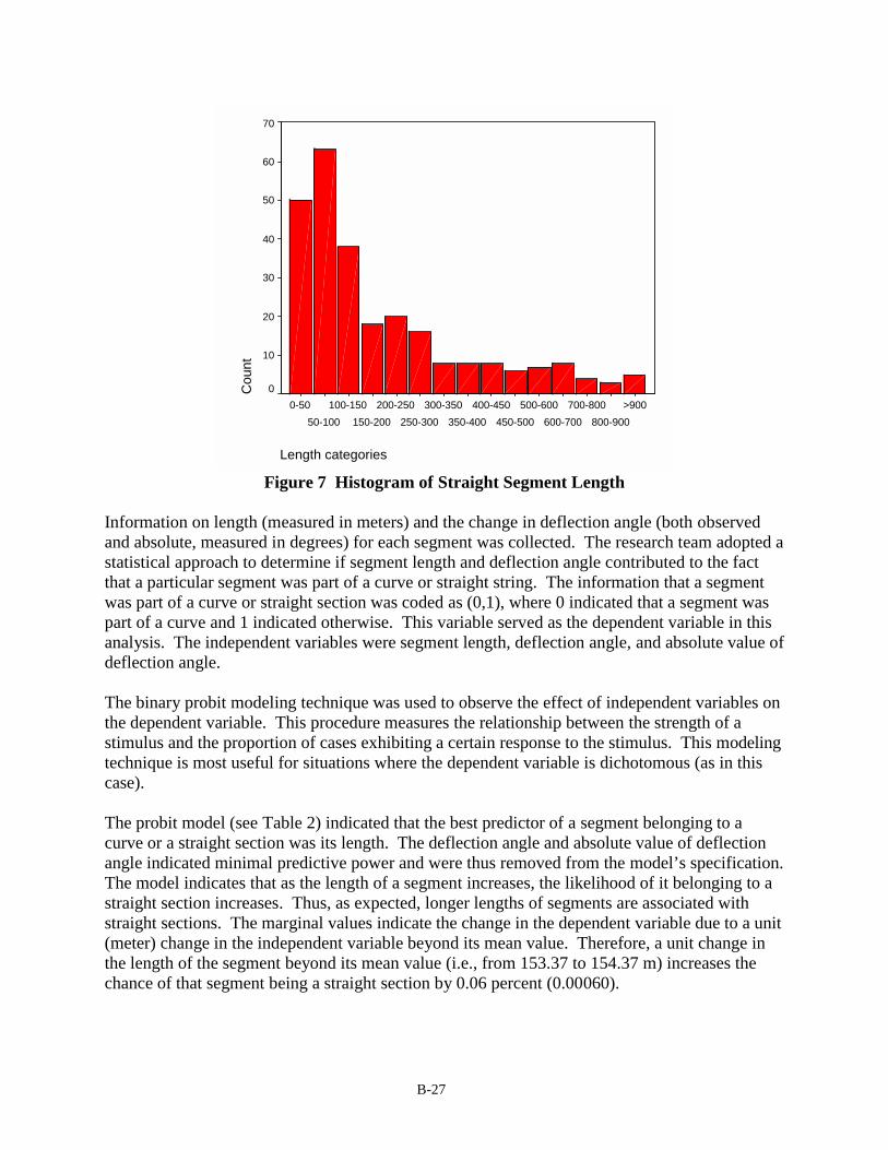
B-27

Length categories

>900

800-900

700-800

600-700

500-600

450-500

400-450

350-400

300-350

250-300

200-250

150-200

100-150

50-100

0-50

Cou

nt

70

60

50

40

30

20

10

0

Figure 7 Histogram of Straight Segment Length

Information on length (measured in meters) and the change in deflection angle (both observedand absolute, measured in degrees) for each segment was collected. The research team adopted astatistical approach to determine if segment length and deflection angle contributed to the factthat a particular segment was part of a curve or straight string. The information that a segmentwas part of a curve or straight section was coded as (0,1), where 0 indicated that a segment waspart of a curve and 1 indicated otherwise. This variable served as the dependent variable in thisanalysis. The independent variables were segment length, deflection angle, and absolute value ofdeflection angle.

The binary probit modeling technique was used to observe the effect of independent variables onthe dependent variable. This procedure measures the relationship between the strength of astimulus and the proportion of cases exhibiting a certain response to the stimulus. This modelingtechnique is most useful for situations where the dependent variable is dichotomous (as in thiscase).

The probit model (see Table 2) indicated that the best predictor of a segment belonging to acurve or a straight section was its length. The deflection angle and absolute value of deflectionangle indicated minimal predictive power and were thus removed from the model’s specification.The model indicates that as the length of a segment increases, the likelihood of it belonging to astraight section increases. Thus, as expected, longer lengths of segments are associated withstraight sections. The marginal values indicate the change in the dependent variable due to a unit(meter) change in the independent variable beyond its mean value. Therefore, a unit change inthe length of the segment beyond its mean value (i.e., from 153.37 to 154.37 m) increases thechance of that segment being a straight section by 0.06 percent (0.00060).

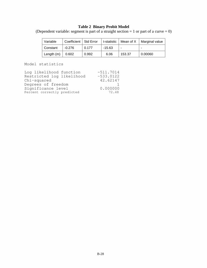
B-28

Table 2 Binary Probit Model(Dependent variable: segment is part of a straight section = 1 or part of a curve = 0)

Variable Coefficient Std Error t-statistic Mean of X Marginal value

Constant -0.276 0.177 -15.63 - -

Length (m) 0.602 0.992 6.06 153.37 0.00060

Model statistics Log likelihood function -511.7014 Restricted log likelihood -533.0122 Chi-squared 42.62147 Degrees of freedom 1 Significance level 0.000000 Percent correctly predicted 72.48

B-29

3.9 Length-based (Defined Interval)

3.9.1 DefinitionThe actual length and end-to-end (straight line) lengths of a selected interval along a string willbe calculated using an Arcview user-code. An interval will be marked as a curve when the actualand end-to-end lengths of the defined interval differ by a selected threshold value. An advantageof this strategy with respect to the “length (string)” technique, is its capability to determine thebeginning and the end points of a curve.

3.9.2 Illustration

4 Curve Identification Strategies Qualitative AssessmentTable 3 Developed and Examined Strategies to Identify Horizontal Curves

StrategiesQuantitative

Assessment (%)Type I Error

(%)Type II Error

(%)

Crash (string) 66 23 11Crash (segment) 68 30 2Bearing-1 See Figure 8*

Bearing-2 No AssessmentManual (string) 85 13 2Manual (segment) 72 28 0Vertex 51 0 49Length (string) 80 19 1Length (segment)** No AssessmentLength (defined interval) No Assessment

* The accuracy level of the strategy was determined for the deflection angles of 1 to 15degrees. As shown in Figure 8, a 74 percent accuracy level (i.e., highest level) isobserved at the 6° deflection angle when the Type I and Type II errors are 8 and 18percent, respectively. However, if the concern is not to miss a curve when actually is acurve (i.e., Type II error), a segment should be tagged as a curve when its deflectionangle is either greater or equal than 1° (or even less than 1° for a lower Type II error).

** The purpose of this strategy was to determine the impact of length and bearing of asegment in identification of curves. A statistical modeling of the bearing and length of

B-30

the identified curves' segments reveals that a segment's length is the best predictor inidentification of curves. The model indicates that as the segment's length increases, thelikelihood of it belonging to a non-curve string increases. The data manipulation andstatistical modeling of this strategy is included in Appendix B.

0

10

20

30

40

50

60

70

80

1 3 5 7 9 11 13 15

Angle (degree)

Per

cen

t

Type I Type II Accuracy

Figure 8 Quantitative Assessment of Bearing-1 Strategy

Appendix CHorizontal Curve Identification Methodology

C-1

1 Curve Identification Technique I

Once the curves' segments have been identified, using the available data sources, thefollowing steps are conducted to calculate curves' radii and degrees:

1. Eliminate the mistakenly selected segments as curves through visual inspections2. Manually put boxes around curves3. Perform clipping

i. Assign a unique number to each polygonii. Assign the polygon unique numbers to the curvesiii. Calculate the length of a curve's segmentsiv. Calculate weighed AADT

4. Combine the clipped segments5. Calculate chord and curve lengths6. Calculate the curves' radii

1.1 Identify ErrorsThe first two main steps are performed manually. In the first step, all selected segmentsare inspected for possible errors. The mistakenly selected segments are eliminated andboxes are put around the remaining curves using the following procedure:

1.2 Draw Boxes Around Curves• Open a new view in ArcView• Add the theme "Co85_prisec.shp"• Open the attribute table of "Co85_prisec.shp"• Query the table to identify road strings with advisory speed limit signs, which are the

indications of presence of curves.• Add a new theme named "Polygon.shp"• Click on Theme on the menu bar• Click on Start Editing• Draw polygons around the identified curves. Each polygon encompasses segments of

a curve from its points of tangency and curvature.

C-2

1.3 Perform ClippingThe purpose of the "clipping" is to isolate the boxes, with their curves within, from therest of the road network.

• Open a new view in ArcView• Add the following themes:

• Polygon.shp - This theme contains the polygons that define the curves in the roadnetwork of the county.

• Co85_prisec.shp - This theme contains the network of primary and secondaryroads in the county

• Select both themes• Click on “Edit” on the menu bar• Click on “Copy Themes”• Click on “Paste”

• Rename “Polygon.shp” and “Co85_prisec.shp” to “Polygon_box.shp” and“Co85_prisec_2.shp”

• Delete the original themes• Click on project window

• Click on “File” on the menu bar• Click on “Extensions”• Click on “Geoprocessing”

• Arrange the themes in the view window such that “Co85_prisec_2.shp” is on top• Click on the view window

• Select all the features of “Polygon_box.shp”• Click on “View” on the menu bar• Click on “Geoprocessing Wizard”• Select the option “Clip one theme based on another”• Click on “Next”• Select “Co85_prisec_2.shp” as the input theme to clip• Select “Polygon_box.shp” as the polygon overlay theme• Specify the location of the output file (e.g., clip2.shp)• Click on “Finish”

C-3

Before combining the curve segments inside each polygon, the following steps need to becarried out:

1.3.1 Assign a unique number to each polygonA unique value is assigned to each polygon. This is an indirect way of numbering thecurves' segments inside the polygon. The following Areview Avenue Script is used toassign numbers to polygons:

thisProject=av.GetProjectthisView=thisProject.FindDoc("View1")themesList=thisView.GetThemesselect theme=MsgBox.ListAsString(themesList,"Themes","Please select")selectTab=selecttheme.getFTabselectTab.seteditable(true)autofield=field.make("Id",#field_decimal,10,0)selectTab.addfields({autofield})autofield.seteditable(true)for each i in selectTabId=i+1SelectTab.setvalue(autofield,i,Id)end

C-4

SHAPE POLYGON_IDPolygon 1Polygon 2Polygon 3Polygon 4Polygon 5Polygon 6Polygon 7Polygon 8Polygon 9Polygon 10Polygon 11Polygon 12Polygon 13Polygon 14Polygon 15

1.3.2 Assign the polygon unique numbers to the curvesIn this step the polygons' unique numbers are assigned to their associated curve'ssegments. This would enable us to integrate the curves' segments based on their uniqueassigned identification numbers. The “assign data by location” option of theGeoprocessing Wizard is used to spatial join the data from the attribute table of curvestheme to the attribute table of “clipped” roads theme.

• Use the curves theme (polygon theme) as the source table and the “clipped” roadstheme (line theme) as the destination table

• Click on “View” on the menu bar• Click on “Geoprocessing Wizard”• Select the option “assign data by location”• Click on “Next”• Select “Clip2.shp” as the theme to be assigned data to• Select “Polygon_box.shp” as the theme to assign data from• Click on “Finish”

1.3.3 Calculate the length of a curve's segmentsA curve length is determined by adding the segments that form the curve inside a box.For those segments that their entire lengths are not included in the box only their partiallengths are considered in calculating the curve length. For example, the selected curve(see the figure below) consists of segments, however, the actual curve length is the onlylength inside the box. Using the following procedure determines the segments' lengthsthat are inside the box. This process would eliminate the over representation of curvelengths.

C-5

• Open the attribute table of “Clip2.shp”

• Click on “Table” on the menu bar• Click on “Start Editing”• Click on “Edit”• Click on “Add Field”• Name the field as “New_length”• Click on “New_length”• Click on “Field” on the menu bar• Click on “Calculate”• [New_length] = [Shape]. RunLength• The new length values are in feet.

1.3.4 Calculate weighted AADTThere are two possible ways to determine a curve AADT (average annual daily traffic).We can simply use the average all segments' AADT that form a curve or more accuratelyuse portions of AADT's of those segments that are partially inside the box. Using thefollowing procedure a curve AADT is determined by weighing the degree of participationof a segment in forming a curve.

• Open the attribute table of “Clip2.shp”• Click on the field “Polygon_id”• Click on “Field” on the menu bar• Click on “Summarize”• The field is “New_Length”• Summarize by sum• Save the summary table to the required location (i.e., Sum_New_length.dbf)• Using the [Polygon_id] as a common field, join the Sum_New_length.dbf and the

attribute table of “Clip2.shp”• The destination table is the attribute table of “Clip2.shp”• Click on “Edit”• Click on “Add Field”• Name the field as [Weighted_Aadt]• Click on “Field” on the menu bar• Click on “Calculate”

• Enter [Aadt]h][Sum_lengt

h][New_lengt]_[ ×

=AadtWeighted

C-6

AADT NEW_LENGTH POLYGON_ID SUM_NEW_LENGTHWEIGHTED_AADT1100 263.411 6 432.9690 6691100 169.558 6 432.9690 43180 67.095 1 129.0660 4280 61.971 1 129.0660 3825 347.908 2 347.9080 2525 116.539 3 290.9110 1025 174.372 3 290.9110 1525 21.303 5 223.4310 225 108.383 5 223.4310 1225 93.089 4 197.0410 1225 93.745 5 223.4310 1025 103.952 4 197.0410 13

1.4 Combining the Clipped SegmentsThe next step is to combine the boxed curves' segments to create polylines.

• Click on “View” on the menu bar• Click on “Geoprocessing Wizard”• Select the option “Dissolve features based on an attribute”• Click on “Next”• Select “Clip2.shp” as the theme to dissolve• Select “Polygon_id” as the attribute to dissolve• Specify the output file location (e.g, Dissolve1.shp)• Click on “Next”• For the additional fields to be included in the output file choose:• New_length by sum• Weighted_Aadt by sum• Index by First• Index by Last• Click on “Finish"

1.5 Calculate chord and curve lengthsThe length and chord length of a curve calculation will be enable us to determine thecurves' radii. The lengths can be calculated using an ArcView Avenue Script.

thisProject=av.GetProjectthisView=thisProject.FindDoc("View1")themesList=thisView.GetThemesselect theme=MsgBox.ListAsString(themesList,"Themes","Please select")selectTab=selecttheme.getFTabselectTab.seteditable(true)chLengthField=field.make("Chord_length",#field_decimal,10,4)

C-7

selectTab.addfields({chLengthField})chLengthField.seteditable(true)for each r in selectTabsegmentPolyLine=selectTab.ReturnValue(selectTab.FindField("Shape"),r)segmentLine=segmentPolyLine.AsLinesegmentStartPoint=segmentLine.ReturnStartsegmentEndPoint=segmentLine.ReturnEndChord_length=segmentStartPoint.Distance(segmentEndPoint)selectTab.setvalue(chLengthField,r,Chord_length)end

POLYGON_ID COUNT FIRST_INDEX WEIGHTED_AADT CHORD_LENGTH CURVE_LENGTH1 2 856502085230603 79.0000 126.2407 129.0660

2 1 856502085230710 78.0000 347.9076 347.9080

3 2 856502085230710 67.0000 287.6124 290.9110

4 2 856502085231806 17.0000 195.9667 197.0410

5 3 856502085231806 4.0000 217.5339 223.4310

6 2 856402085241312 1462.0000 430.1336 432.9690

7 2 856402085241312 882.0000 439.8060 442.9150

8 1 856502085231602 10.0000 139.2522 139.2520

1.6 Calculate the Curves' RadiiThis step was described in the text.1.6.1 Roadware DataIn cases where Roadware data are available, a new ArcView Roadware Theme isgenerated to convert divided roadways into single routes to prevent double counting ofthe clipped segment lengths.

• Open the project “Clip.apr”• Add a new view and name it “Id Using Roadware”• Add the theme “Roadware85.shp”• Open the attribute table of “Roadware85.shp”• The Roadware network consists of bi-directional routes for divided roadways. They

are represented as direction 5 and direction 6. Only a small number of locations arerepresented by direction 6, thus, direction 6 is selected for the elimination.• Query the attribute table for route 5 by setting [Dir1] = 5• Convert the selected set to a shapefile

• Click on Theme on the menu bar• Click on “Convert to a shapefile”• Name the shapefile as “New_Roadware.shp”

• Open the attribute table of “New_Roadware.shp”• Add the theme “Polygon_box.shp”• Open the attribute table

C-8

The clipping procedure, using the Roadware data, somewhat similar to the clipping ofsegments in cartography files.

• Open the attribute table of “Polygon_box.shp”• Perform query by setting [Dfbearing] >=1 or [Dtbearing] >=1 to identify curves• Start GeoProcessing

• Click on project window• Click on “File” on the menu bar• Click on “Extensions”• Click on “GeoProcessing”

• Arrange the themes in the new window such that “New_Roadware.shp” is on top• Click on the view window

• Select all the features of “Roadware_box.shp”• Click on “View” on the menu bar• Click on “GeoProcessing Wizard”• Select the option “Clip one theme based on another”• Click on “Next”• Select “New_Roadware.shp” as the input theme to clip• Select “Roadware_box.shp” as the polygon overlay theme• Specify the location of the output file with the file name (e.g., clip3.shp)• Click on “Finish”

Using the following procedure, the weighted AADT calculated through the use ofcartography files, is incorporated into the roadway data.

• Open the attribute tables of “Dissolve3.shp” and “Final_Dissolve_Rw.shp”• Use the [Polygon_id] as a common field to join the two attribute tables• Hide all fields in “Dissolve3.shp” except [Polygon_id] and [Weighted_Aadt]• The destination table would be the attribute table of “Final_Dissolve_Rw.shp”

2 Curve Identification Technique II

2.1 Identify All Crashes Reported as Occurring on a Curve• Select all primary road crashes, reported by the officer in the field as occurring on a

curve.

([Road_class]<=2) and (([Road_geome]=4) or ([Road_geome]=5) or ([Road_geome]=6))

Note: This selection set limits the primary roadways evaluated by identifying potentialproblem curves or continuous adjacent curves.

2.2 Assign "Curve" Crashes to Roadway Centerline• Using the [Shape] field, spatially join roadway centerline segments to the selected

"curve" crashes.

C-9

• Summarize the joined table using the [Road_link] (unique Base Record segmentidentifier). This yields a table containing a [Road_link] value and correspondingnumber of crashes occurring on the roadway segment, [Count].

• Join the summary table, using [Road_link], to the roadway centerline theme.

2.3 Identify Curves and/or Curve Influence Areas• Visually inspect, systematically, each potential curve site. For example, this may be

accomplished by sorting the summary table by [Count] or [Co].• Select the first record in the list and fit in the "View" window.• While displaying both the "curve" crashes and roadway centerline themes, place

polygons around isolated curves, consecutive curves, and curve influence areas.

Note:• Given that crashes occurring on a curve often do not fall exactly on its cartographic

representation, polygons are drawn in a manner as to include the crashes that shouldfall along this alignment.

• If an intersection occurs along a curve, a portion of the intersection road may beincluded in the polygon.

The remaining steps, beginning with "perform clipping", are essentially the same as curveidentification technique - version 1, with two primary exceptions:

• A spatial join between the curve polygons and crashes is utilized to assign a polygonidentifier to each crash feature. Use of the polygon features, instead of linear curvefeatures, was deemed appropriate given the likelihood of crashes not falling along thecartographic representation of the curve. Since the polygon identifier and curveidentifier are the same for a given location, the ID value may still be used to assignand summarize crash data to the respective curves.

• Crash rates, and rankings, are performed both with and without intersection crashes.Crashes are not limited to those defined as crashes having occurred on a curve.

Appendix DProcedures

Statewide Horizontal Curves With High CrashOccurrences

Statewide Fixed-object Crash Locations

Intersection Crashes along Rural Four-Lane Expressways

Centerline Crossing Head-on Crash Locations on RuralTwo-Lane Paved Road

Four-Lane Undivided Corridors with High CrashOccurrences

D-1

1 Statewide Horizontal Curves (Using Roadware Data)

1.1 Draw Polygons around Curves1.1.1 Objective• To identify curves on the primary road network of the State of Iowa.1.1.2 Process• Open a new view in Arc View by creating a new project "latest_curves.apr"

• Add the theme “Rw00_pri_utm.shp” (This theme contains the roadware data foryear 2000)



• Add the theme “Tenyearcrashes_89-98.shp” (This theme contains the crashesthat occurred on the road network of the state of Iowa from 1989 through 1998)

• Query “Tenyearcrashes_89-98.shp” for primary, non-intersection crashes (The queryis: Road_class = 1 or Road_class = 2 and Int_class = 0). Save the selected set of crashrecords as “Pri_nonint_89-98.shp”

• Create a new polygon theme named “Rdware_polygon.shp” and create a new linetheme named “Rdware_digi_curve.shp”

• Query “Rw00_pri_utm.shp” and “Rw99_pri_utm.shp” for Dfbearing > 1 (This willselect only those road segments which have a bearing greater than 1 with thesucceeding segment). This query helps for relatively easy identification of curves.

• In case of continuous roadware data, visually identify curves on the roadware dataand draw polygons around the curves by editing the theme ‘Rdware_polygon.shp’.Draw the polygons in such a way that the crashes occurring on curves are within thepolygons. Also, draw the polygons in such a way that the primary road network(‘primary_road.shp’) closest to the potential curves on the roadware, falls within thepolygons. Draw polygons only from the point of curvature (PC) to the point oftangency (PT) of the curves. Do not include right angle turns as curves.

• When roadware data is not continuous, manually digitize curves by editing the theme"Rdware_digi_curve.shp".

• Add a column to the attribute tables of both "Rdware_polygon.shp" and"Rdware_digi_curve.shp" to indicate whether the identified curve is a single curve ora set of multiple curves (if applicable).

• Create a new polygon theme and name it as "Digicurve_polygon.shp". Drawpolygons around the manually digitized curves of "Rdware_digi_curve.shp" byediting the theme "Digicurve_polygon.shp".

1.2 Clip Road Network with Polygons1.2.1 ObjectiveTo isolate curves from the road network

D-2

1.2.2 Process• Using Geo processing wizard, clip the primary road network ("primary_road.shp")

with roadware polygons ("Rdware_polygon.shp"). Name the clipped theme as"Rdware_carto_clip.shp". Join the table "aadt_laneleng.dbf" to the attribute table of"Rdware_carto_clip.shp". The objective of clipping and joining is to associate Aadtvalues to the roadware curves in the roadware polygons.

• Using Geo processing wizard, clip the primary road network ("primary_road.shp")with roadware polygons ("Digicurve_polygon.shp"). Name the clipped theme as"manual_carto_clip.shp". Join the table ‘aadt_laneleng.dbf’ to the attribute table of"manual_carto_clip.shp". The objective of clipping and joining is to associate Aadtvalues to the manually digitized roadware curves.

1.3 Assign Unique Value to each Polygon1.3.1 ObjectiveTo be able to identify each polygon with a unique number1.3.2 WhyTo be able to indirectly assign unique numbers to all the curves. A segment or sets ofsegments contained in one polygon and constituting a curve get the same unique id as thepolygon.1.3.3 Process• Run the following Avenue Script on "Rdware_polygon.shp" and

"Rdware_digi_curve.shp" to assign unique values to all the polygonsthisProject=av.GetProjectthisView=thisProject.FindDoc("View1")themesList=thisView.GetThemesselecttheme=MsgBox.ListAsString(themesList,"Themes","Please select")selectTab=selecttheme.getFTabselectTab.seteditable(true)autofield=field.make("Id",#field_double,10,0)selectTab.addfields({autofield})autofield.seteditable(true)for each i in selectTabId=i+1SelectTab.setvalue(autofield,i,Id)End

1.4 Assign Polygon Ids to Cartographic Curves1.4.1 ObjectiveTo assign unique polygon id to each of the cartographic curve segments1.4.2 WhyAll the curve segments would be associated with a polygon id corresponding to thepolygon they belong to. This would help in integration of all the curve segments based onthe unique id assigned to them.Process

D-3

Using the assign data by location option in Geo processing wizard, assign polygon ids tocurves. First, assign data to "Rdware_carto_clip.shp" from "Rdware_polygon.shp" andthen assign data to "manual_carto_clip.shp" from "Digicurve_polygon.shp".

1.5 Calculate Length of Cartographic Curve Segments1.5.1 ObjectiveTo calculate segment lengths for all cartographic curves.1.5.2 WhySome of the curves consist of two or more road segments. In some of these curves, theentire length of the segment is not a part of the curve. Hence, the length of such roadsegments is essential in order to eliminate the over representation of curve length.1.5.3 Process• Calculate the length of each segment of the curve using the function:

Segment length = [Shape]. ReturnLength. Calculate segment lengths for both"Rdware_carto_clip.shp" and "manual_carto_clip.shp". The segment length valuesare in meters.

1.6 Calculate Weighted AADT for Cartographic Curves1.6.1 ObjectiveTo calculate the weighted Average Annual Daily Traffic(AADT) of each road segment ofevery cartographic curve.1.6.2 WhyThe given Aadt of each road segment is for the entire segment. But, the lengths of someof the segments constituting the curves are less than their original lengths. This is due tothe fact that not all segments have their total lengths as part of the curve. Hence, theoriginal Aadt cannot be applied for calculation of the total Aadt of the curve. Theweighted Aadt is more appropriate.1.6.3 Process• In order to calculate the weighted Aadt of each segment, first calculate the total

length of each curve by summarizing the attribute tables of "Rdware_carto_clip.shp"and "manual_carto_clip.shp" on Polygon Id with Segment Length as the summaryattribute. Name the summary table of "Rdware_carto_clip.shp" as"Rdware_sum_newlength.dbf" and the summary table of "manual_carto_clip.shp" as"Manual_sum_newlength.dbf".

• Join "Rdware_sum_newlength.dbf" to the attribute table of "Rdware_carto_clip.shp"using Polygon Id. Similarly join "Manual_sum_newlength.dbf" to the attribute tableof "manual_carto_clip.shp".

• Calculate the weighted Aadt of each of the segments using the formula:

Weighted Aadt = [Aadt]lengthTotal

lengthSegment ×

D-4

1.7 Clip Roadware Data Network with Polygons1.7.1 ObjectiveTo isolate roadware curves from the roadware data network.1.7.2 Process• Using Geo processing wizard, clip the roadware data network ("Rw00_pri_utm.shp")

with roadware polygons ("Rdware_polygon.shp"). Name the clipped theme as"Rw00_curve_clip.shp". Similarly clip the roadware data network("Rw99_pri_utm.shp") with roadware polygons ("Rdware_polygon.shp"). Name theclipped theme as "Rw99_curve_clip.shp".

1.8 Assign Polygon Ids to Polygon Based Roadware Curves1.8.1 ObjectiveTo assign unique polygon id to each of the polygon based roadware curve segments.1.8.2 WhyAll the curve segments would be associated with a polygon id corresponding to thepolygon they belong to. This would help in integration of all the curve segments based onthe unique id assigned to them.1.8.3 Process• Using the assign data by location option in Geo processing wizard, assign polygon ids

to roadware curves. First, assign data to "Rw00_curve_clip.shp" from"Rdware_polygon.shp" and then assign data to "Rw99_curve_clip.shp" from"Rdware_polygon.shp ".

• Some polygon ids could be common between "Rw00_curve_clip.shp" and"Rw99_curve_clip.shp" because of the overlap of the roadware data network of 2000(“Rw00_pri_utm.shp” ) and the roadware network of 1999 (“Rw99_pri_utm.shp”). Inorder to eliminate the common polygon ids, first calculate the count of polygons bysummarizing the attribute tables of "Rdware00_curve_clip.shp" and"Rdware99_curve_clip.shp" on Polygon Id. Name the summary table of"Rdware00_curve_clip.shp" as "Summary_00_clip.dbf" and the summary table of"Rdware99 _curve_clip.shp" as "Summary_99_clip.dbf". Then, join"Summary_00_clip.dbf" and "Summary_99_clip.dbf" to the attribute table of"Rdware00_curve_clip.shp" based on polygon id. Finally, query the attribute table of"Rdware00_curve_clip.shp" as follows: Count00 > 0 and Count99 > 0. The selectedrecords are the common polygon ids. Delete the selected records.

1.9 Assign Polygon Ids to Manual Roadware Curves1.9.1 ObjectiveTo assign unique polygon id to each of the manual roadware curve segments.1.9.2 WhyAll the curve segments would be associated with a polygon id corresponding to thepolygon they belong to. This would help in integration of all the curve segments based onthe unique id assigned to them.

D-5

1.9.3 Process• Using the assign data by location option in Geo processing wizard, assign polygon ids

to manual roadware curves. Assign data to "Roadware_digi_curve.shp" from"Digicurve_polygon.shp".

1.10 Calculate Weighted AADT for Roadware Curves1.10.1 ObjectiveTo calculate the weighted Average Annual Daily Traffic (AADT) of each road segmentof every roadware curve.1.10.2 WhyThe given Aadt of each road segment is for the entire segment. But, the lengths of someof the segments constituting the curves are less than their original lengths. This is due tothe fact that not all segments have their total lengths as part of the curve. Hence, theoriginal Aadt cannot be applied for calculation of the total Aadt of the curve. Theweighted Aadt is more appropriate.1.10.3 Process• In order to calculate the weighted Aadt of each segment, convert

"Rdware_carto_clip.shp" to "Rdware_wtd_aadt.shp" and "manual_carto_clip.shp" to"manual_wtd_aadt shp". Then, join the attribute table of "Rdware_wtd_aadt.shp" to"Rw00_curve_clip.shp", the attribute table of "Rdware_wtd_aadt.shp" to"Rw99_curve_clip.shp", and the attribute table of "manual_wtd_aadt.shp" to"Rdware_digi_curve.shp".

1.11 Dissolve Roadware Curve Segments1.11.1 ObjectiveTo integrate the road segments of every curve.1.11.2 WhyEvery curve could be made up of two or more road links. In order to represent the curveas one individual road segment, the dissolve is essential.1.11.3 Process• Using the dissolve features option in Geo processing wizard, dissolve the roadware

curves. First, dissolve "Rdware_digi_curve.shp" based on polygon id and addweighted Aadt by sum and name it "Manual_dissolve.shp". Similarly, dissolve"Rw00_curve_clip.shp" and name it "Rdware00_dissolve.shp". Also, dissolve"Rw99_curve_clip.shp" and name it "Rdware99_dissolve.shp".

1.12 Calculate Length of Roadware Curve Segments1.12.1 ObjectiveTo calculate curve lengths for all roadware curves.1.12.2 Process• Calculate the length of each curve using the function:

D-6

Curve length = [Shape]. ReturnLength. Calculate curve lengths for"Manual_dissolve.shp", "Rdware00_dissolve.shp", and "Rdware99_dissolve.shp".The curve length values are in meters.

• If weighted Aadt is zero for any of the curves, perform a visual inspection of thosecurves and replace zero Aadt value with the Aadt of the nearest primary roadsegment.

1.13 Calculate Chord Length for Roadware Curves1.13.1 ObjectiveTo calculate the chord length of each roadware curve.1.13.2 WhyOnce the length and chord length of a curve are calculated, the radius of curvature couldbe calculated and hence the chord length is essential.1.13.3 Process• Run the following Avenue Script on "Manual_dissolve.shp",

"Rdware00_dissolve.shp", and "Rdware99_dissolve.shp" to calculate the chord lengthof each curve

thisProject=av.GetProjectthisView=thisProject.FindDoc("View1")themesList=thisView.GetThemesselecttheme=MsgBox.ListAsString(themesList,"Themes","Please select")selectTab=selecttheme.getFTabselectTab.seteditable(true)chLengthField=field.make("Chord_length",#field_double,10,4)selectTab.addfields({chLengthField})chLengthField.seteditable(true)for each r in selectTabsegmentPolyLine=selectTab.ReturnValue(selectTab.FindField("Shape"),r)segmentLine=segmentPolyLine.AsLinesegmentStartPoint=segmentLine.ReturnStartsegmentEndPoint=segmentLine.ReturnEndChord_length=segmentStartPoint.Distance(segmentEndPoint)selectTab.setvalue(chLengthField,r,Chord_length)end

1.14 Calculate Radius and Degree of Curvature of Roadware Curves1.14.1 ObjectiveTo calculate the radius and degree of curvature of each roadware curve.1.14.2 Process• Export the dbf tables of "Manual_dissolve.shp", "Rdware00_dissolve.shp", and

"Rdware99_dissolve.shp" into MS-Excel. Name them "Manual_dissolve.xls","Rdware00_dissolve.xls", and "Rdware99_dissolve.xls" respectively.

• Using the formulas in "degree.xls" or "radius.xls" calculate the radius and degree ofcurvature for all the roadware curves.

D-7

• For curves with radius and/or degree value less than or equal to zero, replace theradius and degree values with 99999.

• Convert "Manual_dissolve.xls" to "Manual_degree.dbf". Similarly, convert"Rdware00_dissolve.xls" to "Rdware00_degree.dbf", and "Rdware99_dissolve.xls" to"Rdware99_degree.dbf".

1.15 Generate Statewide Roadware Curve Database1.15.1 ObjectiveTo generate the statewide roadware curve database by merging the three differentroadware curve databases.1.15.2 Process• Add "Manual_degree.dbf", "Rdware00_degree.dbf", and "Rdware99_degree.dbf"

tables to the Arc View Project "latest_curves.apr".• Join "Manual_degree.dbf" to the attribute table of "Manual_dissolve.shp" based on

polygon id. Similarly, join "Rdware00_degree.dbf" to the attribute table of"Rdware00_dissolve.shp", and "Rdware99_degree.dbf" to the attribute table of"Rdware99_dissolve.shp".

• Add a source field to the attribute tables of "Manual_dissolve.shp","Rdware00_dissolve.shp", and "Rdware99_dissolve.shp". Name the source for"Manual_dissolve.shp" as 'Manual', for "Rdware00_dissolve.shp" as 'Rd00', and for"Rdware99_dissolve.shp" as 'Rd99'.

• Convert "Manual_dissolve.shp" to "Manual_curves.shp", "Rdware00_dissolve.shp"to "Rdware00_curves.shp", and "Rdware99_dissolve.shp" to "Rdware99_curves.shp"

• Using the merge themes option in Geo processing wizard, merge"Manual_curves.shp", "Rdware00_curves.shp", and "Rdware99_curves.shp". Namethe merge as "Statewide_pri_curves.shp"

1.16 Assign Polygon Ids to Primary Crashes1.16.1 ObjectiveTo assign unique polygon id to all the crashes which occurred on primary curves.1.16.2 WhyAll the crashes occurring on primary curves would be associated with a polygon idcorresponding to the polygon they belong to. This would help in counting the number ofcrashes on each primary curve.Process• Using the assign data by location option in Geo processing wizard, assign polygon ids

to crashes occurring on primary curves. Assign data to "Pri_nonint_89-98.shp" from"Rdware_polygon.shp" and then assign data to "Pri_nonint_89-98.shp" from"Digicurve_polygon.shp". Name the polygon ids from "Rdware_polygon.shp" as'Polygon_id_rd' and the polygon ids from "Digicurve_polygon.shp" as'Polygon_id_man'

• In order to identify the crashes which occurred on the curves on the primary roadnetwork, query the attribute table of "Pri_nonint_89-98.shp" as follows:Polygon_id_rd>0 or Polygon_id_man>0. Save the selected set of crashes as"Pri_curve_crashes.shp".

D-8

• To merge the two different polygon id fields (Polygon_id_rd and Polygon_id_man)into one, query the attribute table of "Pri_curve_crashes.shp" as follows:Polygon_id>0. For the selected set of crashes, calculate ' Polygon_id_rd' ='Polygon_id_man'.

D-9

2 Statewide Fixed-object Crash Locations

2.1 "All" Fixed-object Struck CrashesIdentify fixed-object crashes• Join "A" records shape file and "B" records dbf file• Query the joined "B" table to select statewide fix-object crashes

[fix_obj_st] > 1 OR [acc_type] = 18

• Link the highlighted records in the "B" table to "A" records file (active "B" file andclicked [crash_key] fields)

• Remove all joins in the "B" table• Remove all links in the "B" table• Repeat the procedure for each year (i.e., 1989 through 1998 crash data)• Merge all new linked "A" files to zc1a89_98.shp file using Geoprocess--only fix-

object crashes are contained in the merged file

Merge 1989 through 1998 "B" records• Export the highlighted records in "B" tables to new tables (e.g., b89.dbf, b90.dbf, ….,

b98.dbf)• Add script append.ave located on g drive• Compile and run the script• Save the merged table as b89_98.dbf

Merge 1989 through 1998 "C" records--needed for the [severity] field (e.g., fatal, major,minor, and possible injuries):• Link the highlighted records in each "B" table to its associated "C" table (active "B"

file and clicked [crash_key] fields)• Export the selected records in "C" tables to new tables (e.g., c89.dbf, c90.dbf, ….,

c98.dbf) using the append.ave script after compiling and running the script• Save the merged table as c89_98.dbf

• Join st_road.shp and zc1a89_98.shp (clicked [shape] fields)

Select assigned crash records within given boundaries (rural areas within 50 meters, non-rural areas within 20 meters) that occurred at non-intersection locations:• Rename the newly created [distance] field to [distance_j]• Query the joined zca189_98.shp

([city] = 0 AND [distance_j] <= 50) OR ([city] <> 0 AND [distance_j] <= 20) AND([int_class] = 0)

Calculate dollar loss using the c89_98.dbf table:• Add a new field: [$value]• Query for injury severity: [severity] = 1 (fatal)

D-10

• Field/Calculate to populate the [$value] field for the highlighted records with 800000• Repeat the same procedure for [severity] equals to 2 (major), 3 (minor), 4 (possible),

and 0 (unknown) using 120000, 8000, 2000, and 0; respectively• Summarize based on [crash_key] and add sum for [$value]• Save the summarized table as cost_fo.dbf--this table contains total injury cost for

each crash

• Join cost_fo.dbf and zc1a89_98.shp (clicked [crash_key] fields)• Join table containing [AADT], [IRI], [width], and [year] fields and zc1a89_98.shp

(clicked [road_link] fields)• Convert zc1a89_98.shp to a new shape file: 89_98_fixed.shp--the new shape file

contains all the required fields for ranking high fixed-object crash locations

• Open 89_98_fixed.shp file• Summarize based on [road_link] field• Add averages for [AADT] and [lane_length], and sums for [prop_dmg], and [$value]

fields• Save the new table as rank_fixed.dbf

Create a table for fixed object struck types• Hide all fields except [crash_key] and [fix_obj_st] fields in the b89_98.dbf table• Join b89_98.dbf and 89_98_fixed.shp (clicked [crash_key] fields)• Hide all fields except [road_link] and [fix_obj_st] fields in the joined

89_98_fixed.shp• Export the two fields into a new dbf file: fixed_obj_stk.dbf• Open fixed_obj_stk.dbf in Excel• Create a pivot table; select Road_link for row, fix_obj_stk for column, and count

Road_link for data• Copy and paste each pivot table into a new Excel file and save it as fixed_obj_stk.dbf

• Open fixed_obj_stk.dbf in Arcview• Join rank_fixed.dbf and fixed_obj_stk.dbf tables (clicked [road_link] fields)

• Query the joined rank_fixed.dbf to select the links with more than two fixed-objectcrashes

[count] > 2

• Disjoin rank_fixed.dbf table• Export the highlighted records to rank_fixed_gt2.dbf file• Open rank_fixed_gt2.dbf in Excel• Conduct a ranking according to the Iowa DOT procedure• Open the ranked rank_fixed_gt2.dbf in Arcview• Select the top 30 locations: ([final_rank] < 31)• Export the highlighted records to 30_fixed_gt2.dbf• Join 30_fixed_gt2.dbf and st_road.shp (clicked [road_link] fields)

D-11

• Select the 30 joined records in the st_road.shp• Convert to a new shape file: t_30_fixed_gt2.shp to show the top 30 locations on the

map• Link t_30_fixed_gt2.shp and 89_98_fixed.shp files to inspect the identified high

crash locations

2.2 Utility Pole Struck CrashesIdentify utility pole struck crashes in "B" records• Query b89_98.dbf to select statewide utility pole struck crashes

[fix_obj_st] = 15

• Link the highlighted records in the b89_98.dbf to zc1a89_98.shp (active b89_98.dbfand clicked [crash key] fields)

• Convert zc1a89_98.shp to a new shape file: zc1a89_98_ut.shp• Join st_road.shp and zc1a89_98_ut.shp (clicked [shape] fields)

• Rename the newly created [distance] field to [distance_j]• Query the joined zca189_98_ut.shp

([city] = 0 AND [distance_j] <= 50) OR ([city] <> 0 AND [distance_j] <= 20) AND([int_class] = 0)

• Query b89_98.dbf to select statewide utility pole struck crashes

[fix_obj_st] = 15

• Link the highlighted records in the b89_98.dbf to c89_98.dbf (active b89_98.dbf andclicked [crash key] fields)

• Summarize based on [crash_key] and add sum for [$value]• Save the summarized table as cost_fo_ut.dbf--this table contains total injury cost for

all utility pole crashes

• Join cost_fo_ut.dbf and zc1a89_98_ut.shp (clicked [crash_key] fields)• Convert zc1a89_98_ut.shp to a new shape file: 89_98_fixed_ut.shp--the new shape

file contains all the required fields for ranking high utility pole crash locations• Add [AADT], [lane_length] fields to zc1a89_98_ut.shp using the 89_98_fixed.shp

(clicked [road_link] fields)

• Open 89_98_fixed_ut.shp file• Summarize based on [road_link] field• Add averages for [AADT] and [lane_length], and sums for [prop_dmg], and [$value]

fields• Save the new table as rank_fo_ut.dbf

D-12

• Query the rank_fo_ut.dbf to select the links with more than two utility pole crashes

[count] > 2

• Export the highlighted records to rank_fo_ut_gt2.dbf file• Open rank_fo_ut_gt2.dbf in Excel• Conduct a ranking according to the Iowa DOT procedure• Open the ranked rank_fo_ut_gt2.dbf in Arcview• Select the top 30 locations: ([final_rank] < 31)• Export the highlighted records to 30_fo_ut_gt2.dbf• Join 30_fo_ut_gt2.dbf and st_road.shp (clicked [road_link] fields)• Select the 30 joined records in the st_road.shp• Convert to a new shape file: t_30_fo_ut_gt2.shp to show the top 30 locations on the

map• Link t_30_fo_ut_gt2.shp and 89_98_fixed_ut.shp files to inspect the identified high

crash locations

D-13

3 Intersections along Rural Four-Lane Expressways

3.1 Identify Rural Expressways• Query Iowa DOT roadway centerline theme to select rural expressways. For this

study, rural expressways were defined as non-Interstate roadways with four (or more)lanes located outside of corporate limits.

([Sys]<>1) and ([City]=0) and ([Numlanes]>=4)

3.2 Identify Intersecting (Proximate) Roadways• Select (by Theme) all roadway segments from the centerline theme that are within 16

meters of the rural expressways (previous selection set). This value may be adjusted,but, if too large, too many roadways will be selected.

• Add these records to the existing selection set.• Save all records (rural four-lane expressways and intersecting roadways) as new

theme, “rural_express.shp”, and add to view.

3.3 Identify Rural, Intersection Crashes• Query the GIS-ALAS “A” records theme(s) to select rural, intersection crashes. For

this study, rural, intersection crashes were defined as those indicated as rural, non-interchange crashes possessing a valid intersection node id and intersection classcode. These selection criteria yield all rural, intersection crashes and are not limitedto expressways.

([Rur_urb]=”R”) and ([Int_id]<>999999) and ([Int_class]>0) and(([Road_char]>=11) and ([Road_char]<=14))

• Repeat this query for all “A” record themes containing data from years of interest.

3.4 Identify Rural, Expressway Intersection Crashes• Select (by Theme) all rural, intersection crashes, from the “A” records theme(s),

previous selection set, that are within 50 meters of the rural expressways (selectionset from “Identify Intersecting Roadways”). This selection may yield non-expresswaycrashes as well, specifically intersection crashes occurring along the intersectingroadways.

• Merge selected features from all “A” record themes and save as “int94_98.shp”.(This represents a five-year analysis period.)

• Notes:• A value of 50 meters was utilized because it is approximately equal to the accuracy of

the cartographic data.

3.5 Determine Daily Entering Vehicles (DEV) at Intersections(Note: If DEV is known for all [Int_id], the following procedure is not required.)

D-14

3.5.1 Create Single Point Feature at Intersection Sites• Edit “int94_98.shp” and add a new field: [Coint_id], string(8) or decimal(8).• Update [Coint_id] with the concatenation of [Co] and [Int_id].

• [Co] + [Int_id]

• Using the Geoprocessing Wizard, dissolve rural, expressway intersection crashes by[Coint_id]. Create output file “int94_98x.shp”. Summarize [Prop_dmg] by sum foruse in crash ranking. Crash frequency [Count] is calculated automatically and willalso be used in crash ranking.• Other fields may also be summarized to yield the general intersection physical

characteristics and crash history. In addition, discrepancies among recordingofficers may become apparent through the summary data.

• Potential fields on interest include: [Vehicles] by sum, [Killed] by sum, [Injured]by sum, [Prop_dmg] by sum, [Severity] by minimum, [County] by minimum,[City] by minimum, [Rur_urb] by first, [Route] by first, [Int_class] by average,[Road_class] by average, [Road_char] by average, [Road_geo] by average, and[Locality] by average.

Notes:• This step not only yields a single point feature at each crash site with the selected,

summarized “A” record attributes, but the total number (count) of crashes at thesite as well.

• This step is necessary because the primary emphasis of analysis is location-based,not incident-based. However, for incident-based analysis, all crashes may be tiedback to a specific site using the unique [Coint_id].

• [Int_id] is only unique if proceeded by county number, [Co].• Although infrequent, crashes at a single site may incorrectly posses different

[Coint_id] values, resulting in several disparate locations with the same[Coint_id]. These locations must be assessed independently.

3.5.2 Buffer Intersection Sites• With the “int94_98x.shp” theme active, load, compile, and run “bufferid.ave” script.

• Use the [Cont_id] field to identify output buffers and set buffer radiusapproximately equal to 50 meters (the cartographic accuracy).

• Save buffers as “int94_98buf.shp”.

Notes:• This script creates a buffer around each intersection and assigns [Coint_id] to the

buffer.• The newly created buffers will be used to assign intersection approaches to each

intersection.

D-15

3.5.3 Identify Roadway Segments Intersecting Intersection Buffers• Using the Geoprocessing Wizard, clip the “rural_express.shp” theme with the

“int94_98buf.shp” theme. Save the resulting, partial roadway centerline theme as“re_int.shp”.

3.5.4 Assign Intersection Identifier to Intersection Approaches• Using the Geoprocessing Wizard, assign data by location from the “int94_98buf.shp”

theme to the “re_int.shp” theme.

3.5.5 Calculate Number of Unique Centerline Segments per Intersection• Summarize [Input Shape ID] ([Coint_id]) field of “re_int.shp” theme. Save resulting

dbf file as “re_int_sum.dbf”.

3.5.6 Modify Table Definitions for Approach Assignment• Assign the number of centerline segments to each intersection point feature. This is

accomplished by joining “re_int_sum.dbf” to “re_int” theme, using [Coint_id] andsaving the new theme as “re_int2.shp”. A [Count] field is now present in“re_int2.shp”. This represents the number of unique centerline segments locatedwithin the intersection buffer.

Note:• Centerline segments may not terminate at intersections.

• Edit “re_int2.shp” and add field: [Seg_type], string(1). This field will be populatedwith one of the following: “E” = centerline segment ends/terminates at intersection,“T” = centerline segment continues through intersection, “D” = centerline segmentshould not be associated with intersection.

• Edit “rural_express.shp” and add fields: [Coint_id], string(8) or decimal(8), [Count],decimal(1), and [Seg_type], string(1).

• Create new table, “re_int2_append.dbf”. Add fields: [Road_link], [Coint_id],string(8) or decimal(8), [Count], decimal(1), and [Seg_type], string(1). As necessary,records will be added this table to accurately and completely reflect intersectionapproaches.

3.5.7 Visually Inspect Intersection Sites• Sort “re_int2.dbf” by [Input Shape Id] ([Coint_id]).• Select records (centerlines) possessing the same [Input Shape Id] and fit these records

in the active view. Assess whether the selected records are correctly attributed to theactive intersection.• If a segment is correctly attributed to an intersection, update the [Count] and

[Seg_type] fields accordingly.• If a segment appears to be incorrectly attributed to an intersection, update the

[Coint_id] field with null. This may occur if concurrent segments of roadway(along a common intersection approach) fall within the intersection buffer.

D-16

• If an approach segment appears to be missing, identify the appropriate segment in“rural_express.shp” and update the [Coint_id], [Count], and [Seg_type] fields. Ifthis record has already been assigned to another intersection, update [Road_link],[Coint_id], [Count], and [Seg_type] in the “re_int2_append.dbf” file. This mayoccur if a segment lies within multiple intersection buffers.

• Repeat for all intersections.

3.5.8 Aggregate Intersection Approach Records• Select all records from “re_int2.dbf”, “rural_express.shp”, and “re_int2_append.dbf”

where [Coint_id], or [Input Shape ID], is greater than zero or not null.• Export the selected records from the aforementioned tables to individual dbf files.• Using Microsoft Excel, format and append the exported tables. The final table should

contain the following fields, [Road_link], [Coint_id] ([Input Shape Id]), [Count],[Seg_type], as well as new, blank fields of [Aadt], decimal(8), [Adj_aadt],decimal(8), and [Yr_cnt], decimal(4). Save this table as “int1.dbf”.

3.5.9 Calculate DEV• Within ArcView, join “int1.dbf” with a dbf file containing roadway centerline data,

specifically [Road_link], [Aadt], and [Yr_cnt] fields, using [Road_link]. The[Road_link] field represents the unique, Base Record segment identifier.

• Update the [Aadt] and [Yr_cnt] fields in “int1.dbf” with the values contained in thecorresponding fields from the joined table. If the field names are the same, aliasesmust be assigned to the common fields in one of the tables.

• Select from “int1.dbf” where [Seg_type]=”E”. Calculate [Adj_aadt]=[Aadt]/2.• Switch selection and calculate [Adj_aadt]=[Aadt].• Select none and save table “int1.dbf”.• Summarize “int1.dbf” on [Input Shape Id] ([Coint_id]), calculating [Adj_aadt] by

sum. The resulting [Adj_aadt_sum] field represents intersection daily enteringvehicles (DEV). Save the summary table as “Dev.dbf”.

3.6 Determine Total Injury-related Loss at Intersections• Link GIS-ALAS “C” record table to “int94_98” on [Crash_key]. Only display

[Crash_key] and [Severity] fields from “C” records table.• Select crashes from the merged “A” records which occur in the same year as the

crashes represented in the “C” records table. This query will select both the “A”records of interest as well as the corresponding “C” records.• For example, if the “C” records table is “zc1c1998.dbf”, representing 1998

crashes, perform the following query on the merged “A” records:

(([Crash_key]>=1998000000) and ([Crash_key]<1999000000))

where [Crash_key] is a numeric field.

• Remove all links from the “C” and merged “A” records tables. Clear all selectedrecords (select none) and link a different “C” records table, representing a differentyear, to the merged “A” records.

D-17

• Repeat until the appropriate “C” records for all analysis years have been selected.• Export, from all “C” records tables, all selected records.• Append all newly exported “C” records tables by loading, compiling, and running

“table_append.ave” script. Save appended tables as “sev94_98.dbf”.• Edit “sev94_98.dbf” and add fields: [Coint_id], string(8) or decimal(8), and

[Sev_loss], decimal(8).• Join “int94_98x” to “sev94_98” using [Crash_key] and update [Coint_id] with

[Coint_id] from “int94_98x”.• Open “sev94_98.dbf” in Microsoft Excel. Use an “IF” statement to update [Sev_loss]

based on the value of [Severity], e.g.

[Sev_loss]=IF([Severity]=1,800000,IF([Severity]=2,120000,IF([Severity]=3,8000,2000)))

• Within Excel, create a pivot table report using [Coint_id] as the rows of the table andthe sum of [Sev_loss] as the data. This yields the total Export the pivot table as“sev_loss.dbf”.

3.7 Rank Intersections• Within ArcView, join “sev_loss” and “Dev” to “int94_98x” using [Coint_id].

Note:• Not all records will possess [Adj_aadt_sum] (DEV) or [Sev_loss] values. This

occurs when the location is no longer considered in analysis, or when no injuriesresulted, or were reported, at an intersection.

• Select all records where [Adj_aadt_sum] (DEV) is greater than zero and convert to anew shape file, “int94_98x_sum.shp”

• Open “int94_98x_sum.dbf” in Excel and calculate crash rates and ranks.• For each row:

• Sum the [Sev_loss] and [Sum_prop_dmg] columns. This provides a value fortotal loss [Tot_loss] at the intersection.

• Calculate [Crash_rate] = ([Freq]*[1,000,000])/(365*DEV*5), where thenumber of analysis years equals five.

• Use Excel’s “Rank” function to independently rank intersections by crashrate, crash frequency, and total loss. For example, if [Tot_loss] is located incolumn “B”, and the database contains 353 records, the rank for record one iscalculated using the following expression,

=RANK(B2,$B$2:$B$354).

The expression in this form assigns ranks (sorts) in descending order.

• Calculate the sum the loss, crash rate, and crash frequency ranks.• Rank the sum of all ranks in ascending order. For example, if the sum of

ranks is located in column “O”, the following expression applies,

D-18

=RANK(O2,$O$2:$O$354,1)

This yields the overall ranking of the intersection with respect to all otherintersections.

D-19

4 Centerline Crossing Head-on Crash Locations on RuralTwo-Lane Paved Road

Identify centerline crossing head-on crashes:• Join "A" records shape file and "B" records dbf file• Query the joined "B" table to select statewide fix-object crashes

[driv_veh1] = 7 OR [driv_veh2] = 7 OR [coll_type] = 1

• Link the highlighted records in the "B" table to "A" records file (active "B" file andclicked [crash_key] fields)

• Remove all joins in the "B" table• Remove all links in the "B" table• Repeat the procedure for each year (i.e., 1989 through 1998 crash data)• Merge all new linked "A" files to ho_a89_98.shp file using Geoprocess--only fix-

object crashes are contained in the merged file

Merge 1989 through 1998 "B" records:• Export the highlighted records in "B" tables to new tables (e.g., ho_b89.dbf,

ho_b90.dbf, …., ho_b98.dbf)• Add script append.ave located on g drive• Compile and run the script• Save the merged table as ho_b89_98.dbf

Merge 1989 through 1998 "C" records--needed for the [severity] field (e.g., fatal, major,minor, and possible injuries):• Link the highlighted records in each "B" table to its associated "C" table (active "B"

file and clicked [crash_key] fields)• Export the selected records in "C" tables to new tables (e.g., ho_c89.dbf, ho_c90.dbf,

…., ho_c98.dbf) using the append.ave script after compiling and running the script• Save the merged table as ho_c89_98.dbf

Create a shape file for the identified rural 2-lane paved links• Dissolve st_road.shp based on [mslink] field attribute and save the new file as

st_road_mslink_dissolved.shp• Join rural_2lane_paved.dbf (this is a dbf file that contains all rural 2lane paved links)

and st_road_mslink_dissolved.shp (clicked [mslink] fields)• Query the joined st_road_mslink_dissolved.shp to select the rural 2lane paved links

[surf_type] > 0

• Convert st_road_mslink_dissolved.shp to a new shape file: st_rural_2lane_paved.shp• Disjoin st_road_mslink_dissolved.shp• Delete st_road_mslink_dissolved.shp theme

D-20

• Join st_rural_2lane_paved.shp and ho_a89_98.shp (clicked [shape] fields)

Select assigned crash records within given boundaries (rural areas within 50 meters) thatoccurred at non-intersection locations:• Rename the newly created [distance] field to [distance_j]• Query the joined ho_a89_98.shp

[distance_j] <= 50 AND ([int_class] = 0)

Calculate dollar loss using the c89_98.dbf table:• Add a new field: [$value]• Query for injury severity: [severity] = 1 (fatal)• Field/Calculate to populate the [$value] field for the highlighted records with 800000• Repeat the same procedure for [severity] equals to 2 (major), 3 (minor), 4 (possible),

and 0 (unknown) using 120000, 8000, 2000, and 0; respectively• Summarize based on [crash_key] and add sum for [$value]• Save the summarized table as cost_ho.dbf--this table contains total injury cost for

each crash

• Join cost_ho.dbf and ho_a89_98.shp (clicked [crash_key] fields)• Join table containing [AADT], [IRI], [width], and [year] fields and ho_a89_98.shp

(clicked [road_link] fields)• Convert ho_a89_98.shp to a new shape file: 89_98_ho.shp--the new shape file

contains all the required fields for ranking high head-on crash locations

• Open 89_98_ho.shp file• Summarize based on [road_link] field• Add averages for [AADT] and [lane_length], and sums for [prop_dmg], and [$value]

fields• Save the new table as rank_ho.dbf

• Query rank_ho.dbf to select the links with more than two head-on crashes

[count] > 2

• Export the highlighted records to rank_ho_gt2.dbf file• Open rank_ ho_gt2.dbf in Excel• Conduct a ranking according to the Iowa DOT procedure• Open the ranked rank_ ho_gt2.dbf in Arcview• Select the top 30 locations: ([final_rank] < 31)• Export the highlighted records to 30_ho_gt2.dbf• Join 30_ ho_gt2.dbf and st_rural_2lane_paved.shp (clicked [road_link] fields)• Select the 30 joined records in the st_rural_2lane_paved.shp• Convert to a new shape file: t_30_ho_gt2.shp to show the top 10 locations on the map• Link t_30_ ho_gt2.shp and 89_98_ho.shp files to inspect the identified high crash

locations

D-21

5 Four-Lane Undivided Corridors with High Crash Occurrences

Analysis, entails: 1) defining four-lane, undivided corridors, 2) calculating corridorlength and a weighted AADT for the corridor, and 3) considering all crashes (intersectionand non-intersection) along the corridor in rate determination and ranking.

5.1 Identify Four-lane, Undivided Roadways• Query Iowa DOT roadway centerline theme to select four-lane, undivided roadways.

For this study, four-lane undivided roadways were defined as urban, primaryroadways with four (or more) lanes and no median and annual traffic less than14,000.

([Sys]<=3) and ([Numlanes]>=4) and ([Med_type]=0) and ([City]>0) and([Aadt]<=14000) and ([Func]<50)

• The aforementioned selection should then be further limited by lane type.Specifically, the selection set should only include facilities with four through lanesand no center, bi-direction left turn lane. Given the potential complexity of the query,five lane facilities may require visual inspection of the lane types. In addition, lanetypes may be presented in multiple fields for each lane or a single, combined fieldrepresenting all lanes. For example, to identify all four lane facilities consistingsolely of four through lanes, the following query may be used.

([Lane_type]=”111100000”)

Once again, all five lane facilities should be visually inspected and added to thecurrent selection set as deemed appropriate. (See the Base Record Road andStructure Data Manual for lane type definitions.)

Save results as “undiv4.shp”.

5.2 Define Urban, Four-lane Corridors• Edit “undiv4”. Add “corridor_id” field (number, 4) and “corridor_loc” (string, 10)

field. “Corridor_loc” will serve as a single field indicating the general location of aroadway segment.

• Update “corridor_loc” field with the following:

[Co]+[City]+[St_rte]

• Sort “undiv4” by “corridor_loc”. Select common “corridor_loc” values and view theselection set graphically. Corridors may include adjacent roadway segmentspossessing a different “corridor_id” value. For example, adjacent segments outsideof the corporate limit. Update the “corrider_id” field of these records with a unique,integer value.

D-22

Add “alt_corrid” field (number 4). This field will be used to represent partial corridors(corridor segments). Define these corridor segments based primarily on location,continuity, and homogeneity in traffic and lane type.

5.3 Create Corridor Coverage• Edit “undiv4”. Add field “wt_aadt” (number 5) and “Leng_mi” (number 6,3).• If “Lane_leng” is in meters, update “Leng_mi” with se gment length in miles:

[Lane_leng]*.0006214

• Summarize “undiv4” on “Corridor_id” (lane_mi.dbf):

Lane_mi: sum

Change field name to “Sum_leng_mi”.

• Join “lane_mi.dbf” to “undiv4” on “Corridor_id”. Set “Wt_aadt” equal to thefollowing:

([Leng_mi]/[Sum_leng_mi])*[Aadt]

• Using the Geoprocessing Wizard, dissolve “undiv4” on “corridor_id”.

Road_link: firstLane_leng: sumWt_aadt: sum

Save as: “undiv4_ag.shp”

[Repeat this for the partial corridors (corridor segments), based on “alt_corrid”.]

5.4 Identify Urban, Primary Crashes• Query the GIS-ALAS “A” records theme(s) to select urban, primary road crashes.

For this study, urban, primary road crashes were defined as those indicated asoccurring in a city on an Iowa or US route. This selection criteria yield all urban,primary road crashes and are not limited to four lane, undivided roadways.

(([Rur_urb]=”U”) or ([City]>0)) and ([Road_class]=2)

• Repeat this query for all “A” record themes containing data from years of interest.

5.5 Identify Urban, Primary Crashes on Corridors of Interest• Select (by Theme) all urban, primary crashes, from the “A” records theme(s),

previous selection set, that are within 16 meters of the four lane undivided roadways.

D-23

This selection may yield crashes on adjacent, primary roadways occurring within 16meters of the roadways of interest.

• Merge selected features from all “A” record themes and save as “crashmerge.shp”.(This represents a five-year analysis period.)

Notes:• A value of 16 meters was utilized because it is approximately equal to the accuracy of

the cartographic data.

5.6 Assign Corridor Attributes to Crashes• Using the Geoprocessing Wizard, assign data by location from the “undiv4_ag.shp”

theme to the “crashmerge.shp” theme. The attributes of interest are “wt_aadt”,“lane_leng”, and “corridor_id” (unique segment identifier).


5.7 Determine Total Injury-related Loss along Corridors• Link GIS-ALAS “C” record table to “crashmerge” on [Crash_key]. Only display

[Crash_key] and [Severity] fields from “C” records table.• Select crashes from the merged “A” records which occur in the same year as the

crashes represented in the “C” records table. This query will select both the “A”records of interest as well as the corresponding “C” records.• For example, if the “C” records table is “zc1c1998.dbf”, representing 1998

crashes, perform the following query on the merged “A” records:

(([Crash_key]>=1998000000) and ([Crash_key]<=1999000000))

where [Crash_key] is a numeric field.

• Remove all links from the “C” and merged “A” records tables. Clear all selectedrecords (select none) and link a different “C” records table, representing a differentyear, to the merged “A” records.

• Repeat until the appropriate “C” records for all analysis years have been selected.• Export, from all “C” records tables, all selected records.• Append all newly exported “C” records tables by loading, compiling, and running

“table_append.ave” script. Save appended tables as “inj_sev.dbf”.• Edit “inj_sev” and add fields: [Corridor_id], string(8) or decimal(8), and [Sev_loss],

decimal(8).• Join “crashmerge” to “inj_sev” using [Crash_key] and update [Corridor_id] with

[Coint_id] from “crashmerge”.• Open “inj_sev.dbf” in Microsoft Excel. Use an “IF” statement to update [Sev_loss]

based on the value of [Severity], e.g.

[Sev_loss]=IF([Severity]=1,800000,IF([Severity]=2,120000,IF([Severity]=3,8000,2000)))

D-24

• Within Excel, create a pivot table report using [Corridor_id] as the rows of the tableand the sum of [Sev_loss] as the data. This yields the total Export the pivot table as“sev_loss.dbf”.


5.8 Rank Corridors• Within ArcView, summarize “crashmerge” on “Corridor_id”:

Prop_dmg: sumLeng_mi: firstWt_aadt: first

Save as “crashmerge_sum.dbf”.•

• Within ArcView, join “sev_loss” to “crashmerge_sum” using [Corridor_id]. Exportas “crashmerge_final.dbf”.

• Open “crashmerge_final.dbf” in Excel and calculate crash rates and ranks.• For each row:

• Sum the [Sev_loss] and [Sum_prop_dmg] columns. This provides a value fortotal loss [Tot_loss] at the intersection.

• If Sum_leng_miles is less than 0.6 miles,• [Crash_rate] = ([Freq]*[1,000,000])/(365*Sum_leng_mi*Wt_aadt*5), where

the number of analysis years equals five.• If Sum_leng_miles is greater than or equal to 0.6 miles,• [Crash_rate] = ([Freq]*[1,000,000])/(365*(Sum_leng_mi/0.3)*Wt_aadt*5),

where the number of analysis years equals five.• Use Excel’s “Rank” function to independently rank intersections by crash

rate, crash frequency, and total loss. For example, if [Tot_loss] is located incolumn “B”, and the database contains 353 records, the rank for record one iscalculated using the following expression,

=RANK(B2,$B$2:$B$354).

The expression in this form assigns ranks (sorts) in descending order.

• Calculate the sum the loss, crash rate, and crash frequency ranks.• Rank the sum of all ranks in ascending order. For example, if the sum of

ranks is located in column “O”, the following expression applies,

=RANK(O2,$O$2:$O$354,1)

This yields the overall ranking of the corridors with respect to all othercorridors.

D-25

• Update the named range of the dbf file and save. Join these results to“undiv4_ag” to view the locations spatially.


systematic identification of high crash locations

Documents