technical university of denmark - troels...

Technical University of Denmark

Basilar membrane models

2nd semester project

DTU Electrical Engineering

Acoustic Technology

Spring semester 2008

Group 5

Troels Schmidt Lindgreen – s073081David Pelegrin Garcia – s070610

Eleftheria Georganti – s073203

Instructor

Mørten Løve Jepsen

DTU Electrical Engineering

Ørsteds Plads, Building 348

2800 Lyngby

Denmark

Telephone +45 4525 3800

http://www.elektro.dtu.dk

Technical University of Denmark

Title:

Basilar membrane models

Course:

31236 Auditory Signal Processingand PerceptionSpring semester 2008

Project group:

5

Participants:

Troels Schmidt LindgreenDavid Pelegrin GarciaEleftheria Georganti

Supervisor:

Torsten Dau

Instructor:

Mørten Løve Jepsen

Date of exercise: March 13th

Pages: 23

Copies: 4

Synopsis:

Two linear basilar membrane models are

studied.

The first model (“transmission-line

model”) is based on the mechanical

properties (mass, stiffness and damping)

of different segments along the basilar

membrane and it is implemented as an

electric circuit taking advantage of the

existing electro-mechanical analogies.

Thus, different phenomena are deduced

from the mechanical properties, such

as the travelling wave along the basilar

membrane and the forward spread of

masking.

The second model (“gammatone au-

ditory filterbank”) is an approach to the

tuning properties at different places on the

basilar membrane with the corresponding

delays. It is used to study the energy

distribution of a sound at the different

regions of the basilar membrane as a

function of time.

No part of this report may be published in any form without the consent of the writers.

Introduction

A physical system can be studied analyzing each one of its parts and the relationshipbetween them. Thus, the properties of one of the parts determine some of the proper-ties of the overall system. Applying this study method to the human hearing system, itcan be stated that the outer ear acts as a tube providing resonances and the middle earprovides an impedance matching between different mediums. The inner ear is the placewhere mechanical vibrations are transformed into neural excitation. Therefore, the studyof the elements inside the inner ear can lead to know in which way this transformationtakes place, depending on the excitation signal and level.

In this report, the basilar membrane is studied by means of computer models. A firstmodel is designed according to its mechanical properties in a simplified way, seeing thebasilar membrane as a discrete series of elements with constant mass, but changing stiffnessand damping. The differential equations defining electrical and mechanical magnitudes aresimilar and thus it is possible to establish an analogy between them and in fact, the basilarmembrane model is implemented as an electrical circuit.

A second model is the gammatone auditory filterbank, implemented as a series of parallelband-pass filters that model the tuning frequency at each point of the basilar membraneand take the delay into account, making possible to analyze the excitation patterns pro-duced by a given input signal.

Technical University of Denmark, March 25, 2008

Troels Schmidt Lindgreen David Pelegrin Garcia Eleftheria Georganti

Contents

1 Theory 1

1.1 Transmission-line model . . . . . . . . . . . . . . . . . . . . . . . . . . . . . 11.2 Gammatone auditory filterbank . . . . . . . . . . . . . . . . . . . . . . . . . 4

2 Results 5

2.1 Transmission-line model . . . . . . . . . . . . . . . . . . . . . . . . . . . . . 52.2 Gammatone-filter model . . . . . . . . . . . . . . . . . . . . . . . . . . . . . 11

3 Discussion 17

3.1 Transmission-line model . . . . . . . . . . . . . . . . . . . . . . . . . . . . . 173.2 Gammatone filterbank model . . . . . . . . . . . . . . . . . . . . . . . . . . 183.3 Excitation patterns . . . . . . . . . . . . . . . . . . . . . . . . . . . . . . . . 18

4 Conclusion 21

Bibliography 23

A Matlab Code A1

A.1 GammaIR . . . . . . . . . . . . . . . . . . . . . . . . . . . . . . . . . . . . . A1A.2 Gammatone filterbank . . . . . . . . . . . . . . . . . . . . . . . . . . . . . . A1A.3 Chirp that compensates for the delay of the flters . . . . . . . . . . . . . . . A2

March 2008 Chapter 1. Theory

Chapter 1Theory

1.1 Transmission-line model

The transmission-line model is a simplified model of the basilar membrane (cochlea). Themodel describes the basilar membrane velocity and the force and fluid volume velocitiesin the cochlea. The model can be thought of as a chain of independent mechanical filters,representing different segments along the cochlear partition. [Dau et al., 2008, p. 2]

1.1.1 Toward a model

The form of the cochlea and the structure of the cell aggregates within it are very com-plicated. Thus, some simplifications are made in order to have a tractable model of thecochlea. These simplifications are made over the basis of the following assumptions:

• The fluid in the canals is incompressible and will neglect all viscosity effects in it.

• The movements are so small that the fluid and the basilar membrane operate linearly.

The above assumptions result in the cochlea having a linear behavior, which is not theactual case, but in this report the assumption is sufficient. Because the cochlea is assumedto behave linearly, linear mathematical formulas can be used to describe the system.

Another assumption is that the various parts of the basilar membrane are not mechani-cally coupled to each other and that all coupling occurs via the surrounding fluid. Thismeans that the mechanics of the cochlear partition can be described by a single functionof x, the acoustic impedance ξ(x). [de Boer, 1980, p. 139]

The motion on the basilar membrane is described by a traveling wave, the speed of propa-gation of which decreases with increasing distance x. The one-dimensional approximation

Page 1

Chapter 1. Theory Technical University of Denmark

will only be valid if the dimensions in the y- and z-directions are small compared withthe smallest wavelength in the x-direction. This is assumed in this report as the acousticimpedance is assumed to be a function of only x.

A well-known model for the one-dimensional linear cochlear is the wave equation:

∂2 p(x)∂x2 +

2 jωρh(x)ξ(x)

p(x) = 0 [Dau, 2008, p. 19] (1.1)

Where:p(x) is pressure.ρ is the density of the fluid.h(x) is the effective height.ξ(x) is the acoustic impedance.

It is clear that the solution p(x) critically dependence on the product h(x)ξ(x). h(x) variesslowly with x, so for simplicity it is regarded as a constant, hence the impedance ξ(x) isthe critical factor. The acoustic impedance is composed of three parts, a mass part, adamping part and a stiffness part and is given by:

ξ(x) = jω · m(x) + r(x) +c(x)jω

[de Boer, 1980, p. 141] (1.2)

Where:m(x) is the mass of the considered basilar membrane segment at position x.r(x) is the damping of the considered basilar membrane segment at position x.c(x) is the stiffness of the considered basilar membrane segment at position x.

The stiffness is responsible for the occurrence of the traveling wave propagating alongthe cochlear partition. Due to the variations of the stiffness term, the velocity of propa-gation will greatly depend on x.

1.1.2 Mechanical circuit

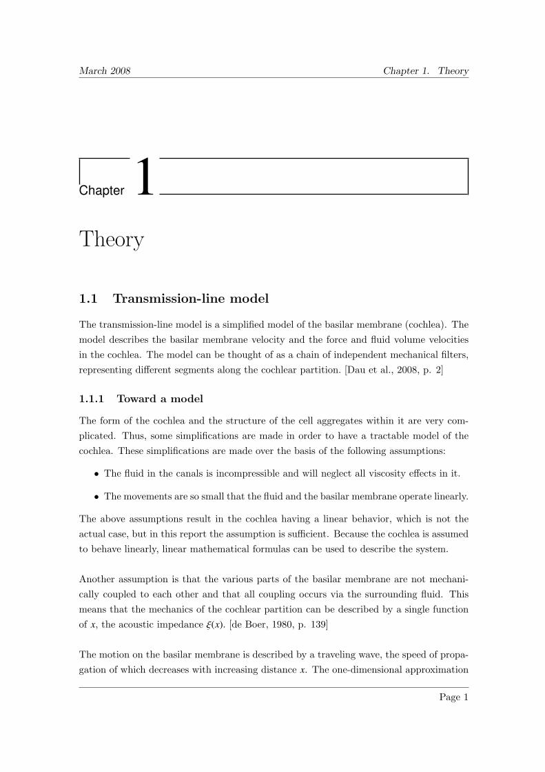
The transmission-line model described by (1.1) can be modeled mechanically as seen onfigure 1.1 [Dau et al., 2008, p. 3].

The fluid pipe in figure 1.1 consists of distributed masses, m1,m3, . . .. A series of resonatorsare connected to taps of the fluid pipe. Each resonator represents a segment on the basilarmembrane and consists of a mass mi, a spring ki and a damper bi.

Page 2 Basilar membrane models

March 2008 Chapter 1. Theory

2 TRANSMISSION-LINE MODEL 1.1 Exercise objectives

1.1 Exercise objectives

After completion of this lab exercise and the associated report it is expected that you should beable to:

• Derive the voltage- and current transfer function of a single segment of the transmission linemodel and evaluate the simulated results with respect to the forces and velocities in thecochlea

• Translate the mechanical transmission line model into the electrical transmission line modeland relate the simulated results to basilar membrane dynamics and auditory filters

• Implement a single gammatone filter in Matlab and determine a relation between its impulseresponse and the centre frequency

• Explain the differences in the excitation pattern of the frequencies in the gammatone filterbank in response to a rising chirp stimulus compared to a click stimulus

• State one characteristic where the transmission line model and the gammatone filter bankdiffer from each other with respect to the shape of the auditory filters

2 Transmission-line model

A strongly simplified mechanical circuit of the cochlea mechanics is shown in Fig. 2. The fluid

m2

k2b2

Fm1

m4

k4b4

m3 mN-1

mN

kNbN

Figure 2.1: Mechanical equivalent circuit of the cochlea. The driving force F is applied at thestapes. The scale vestibuli is modelled as a fluid pipe. The basilar membrane as independent seg-ments. The pressure (force) difference between scala vestibuli and tympani driving the segmentsof the basilar membrane is simplified to a force from the scala vestibuli only.

filled “pipe” consists of distributed masses m1, m3, ... a series of resonators is connected to tapsof the fluid pipe. Each of the resonators is meant to reflect a segment of the basilar membrane.Resonator i consists of a mass mi, a spring ki and a damper bi. As a good first approximation,the fluid pipe can be thought of as the scala vestibuli. The model is driven by a force F appliedto the stapes. This will result in forces applied to each of the resonator segments and the massesalong the pipe. The force applied to a segment will cause all elements of the segment to moveat a certain velocity. Assuming F varies harmonically as F0e

jωt, the velocity vi of element i canbe obtained from the force Fi applied to element i and the mechanical impedance of the element

3

Figure 1.1: Mechanical equivalent circuit of the cochlea. The driving force F is applied at the stapes. Thescala vestibuli is modeled as a fluid pipe and the basilar membrane as independent segments.

The model is driven by a force F applied to each resonator segments and the massesalong the pipe. The force applied to a segment will cause all elements of the specificsegment to move at a certain velocity.

1.1.3 Electric circuit

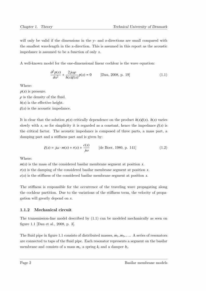
To implement and analyze the transmission-line model it is advantageous to translate themechanical model into an equivalent electric circuit model by using an electro-mechanicalanalogy. The relationship between mechanical and electric elements can be seen in table1.1.

Element type Electrical MechanicalName Impedance Name Impedance

Effort source Voltage (V) Force (F)Flow source Current (I) Velocity (v)Flow storage Inductor (L) jωL Mass (m) jωmEffort storage Capacitor (C) 1/( jωC) Spring (k) k/( jω)Dissipator Resistor (R) R Damper (b) b

Table 1.1: Summery of equivalent elements in the electro-mechanical analogy. From [Dau et al., 2008, p.4].

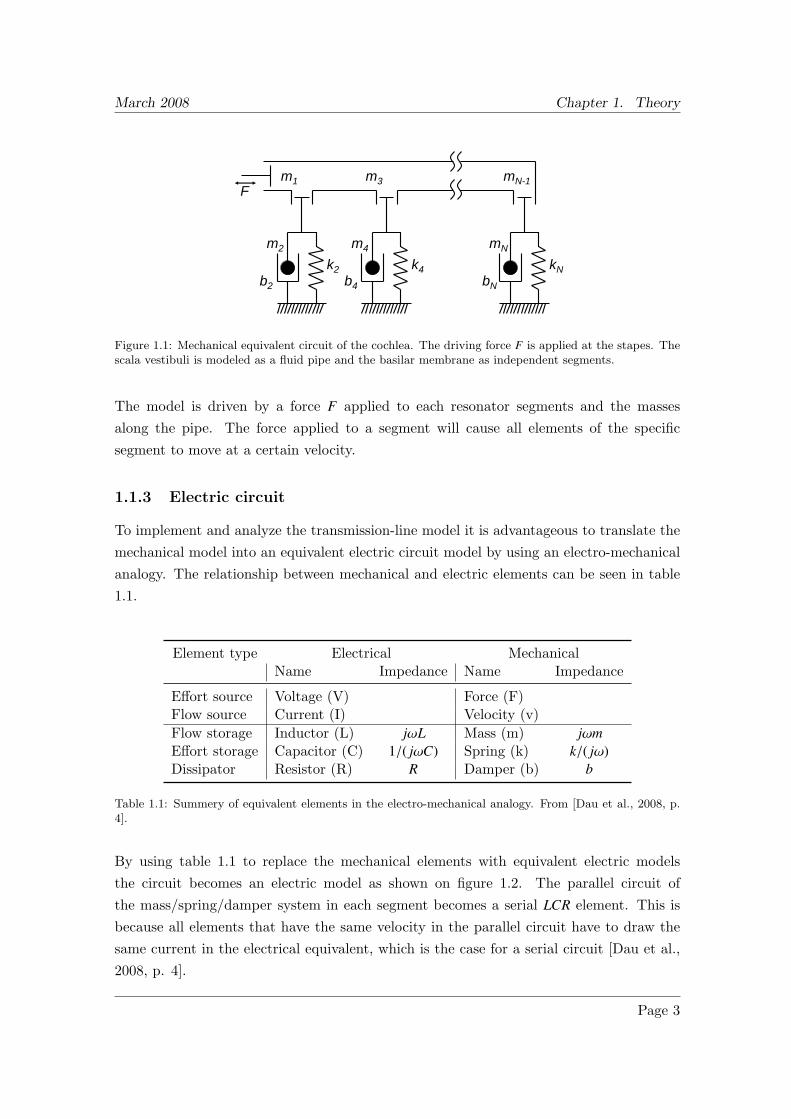
By using table 1.1 to replace the mechanical elements with equivalent electric modelsthe circuit becomes an electric model as shown on figure 1.2. The parallel circuit ofthe mass/spring/damper system in each segment becomes a serial LCR element. This isbecause all elements that have the same velocity in the parallel circuit have to draw thesame current in the electrical equivalent, which is the case for a serial circuit [Dau et al.,2008, p. 4].

Page 3

Chapter 1. Theory Technical University of Denmark

2 TRANSMISSION-LINE MODEL

Zi:

vi =Fi

Zi

. (2.1)

The mechanical impedance is frequency dependent and defined for each element i as:

Zi(s) = mis +ki

s+ bi , (2.2)

where s is the complex frequency variable s = jω. These type of equations can be solved forthe whole model. The solution describes the velocity and forces at all segments along the basilarmembrane.In this exercise you will build your own transmission line model by using the electrical circuit ana-lyzer Pspice Student. Therefore, the mechanical model has to be translated into an equivalentelectrical circuit. We use the first electro-mechanical analogy (voltage/force) from the lecture.Table 2 shortly summarizes the relationship between the mechanical and electrical elements.The mechanical circuit is then translated into the electrical equivalent circuit shown in Fig. 2 All

Element type Electrical MechanicalName Impedance Name Impedance

Effort source voltage[U] force[F]Flow source current[I] velocity[v]Flow storage inductor[L] Ls mass[m] msEffort storage capacitor[C] 1/Cs spring[k] k/s

Dissipator resistor[R] R damper[b] b

Table 2.1: Summary of equivalent elements in the first electro-mechanical analogy. s representsthe complex frequency variable jω.

L1 L3 LN-1

L2

C2

R2

UL4

C4

R4

LN

CN

RN

Figure 2.2: Equivalent electrical circuit for the mechanical model of the cochlea in Fig. 2.

masses are replaced by inductors Li, the compliances of springs are replaced by capacitors Ci andthe dampers are replaced by resistors Ri. The parallel circuit of the mass/spring/damper systembecomes a serial LCR element. This is because all elements that have the same velocity in theparallel mechanical circuit have to draw the same current in the electrical equivalent, which isthe case for a serial circuit.

4

Figure 1.2: Equivalent electric model for the mechanical model in figure 1.1. From [Dau et al., 2008, p. 4].

1.2 Gammatone auditory filterbank

The gammatone auditory filterbank is a set of band-pass filters designed to characterisethe nerve impulse responses to sounds, originally studied with experiments in cats [Dauet al., 2008, p. 6]. Each filter (centered at frequency fc) has an impulse response given by:

g(t) = a−1e(t) cos(2π fct + φ), t > 0, (1.3)

where φ is the phase of the carrier (cosine) relative to e(t), the envelope function of thefilter, and a is a normalization constant, calculated as follows:

e(t) = tn−1e−2πbt (1.4)

a =

∫ ∞

0e(t)dt (1.5)

In these equations, n is the order of the filter, which indicates the slope of the skirts of thefilter and b is a parameter that determines its time duration and the delay of the response.A value of n = 4 is assumed in this exercise, because in this range the shape of the filteris similar to the round exponential filter, which is used to approximate the magnitude ofthe human auditory filter characteristic.

The equivalent rectangular bandwidth (ERB) is a way to quantify the bandwidth of hu-man filters at center frequencies fc. The ERB is the bandwidth of a rectangular filterwhich has the same energy as a given auditory filter. The ERB as a function of the centerfrequency of the filter is estimated to be:

ERB = 24.7 + 0.108 fc (1.6)

In the present laboratory exercise, b = 1.018 ERB.


March 2008 Chapter 2. Results

Chapter 2Results


2.1.1 Analytical analysis of a single segment

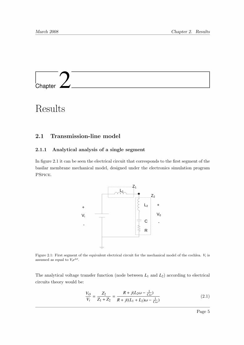
In figure 2.1 it can be seen the electrical circuit that corresponds to the first segment of thebasilar membrane mechanical model, designed under the electronics simulation programPSpice.

L1

L2

C

R

Vi V0

+

-

+

-

Z1

Z2

Figure 2.1: First segment of the equivalent electrical circuit for the mechanical model of the cochlea. Vi isassumed as equal to Vie jωt.

The analytical voltage transfer function (node between L1 and L2) according to electricalcircuits theory would be:

VO

Vi=

Z2

Z1 + Z2=

R + j(L2ω −1

Cω )

R + j((L1 + L2)ω − 1Cω )

(2.1)

Page 5

Chapter 2. Results Technical University of Denmark

Additionally the analytical transfer function for the current equals to:

I0

Vi=

1

R + j((L1 + L2)ω − 1

ωC

) (2.2)

Equation (2.1), which is the transfer function for the voltage equals a low pass filter,whereas the transfer function of the current equals a bandpass filter.

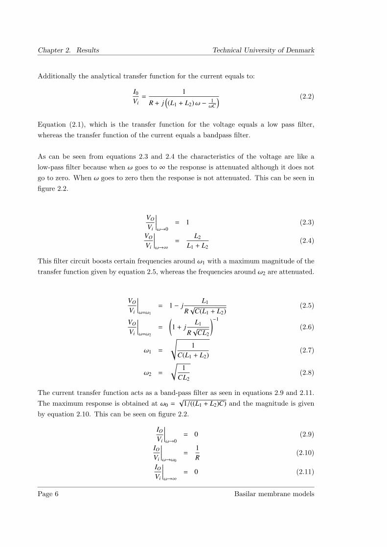
As can be seen from equations 2.3 and 2.4 the characteristics of the voltage are like alow-pass filter because when ω goes to ∞ the response is attenuated although it does notgo to zero. When ω goes to zero then the response is not attenuated. This can be seen infigure 2.2.

VO

Vi

∣∣∣∣∣ω→0

= 1 (2.3)

VO

Vi

∣∣∣∣∣ω→∞

=L2

L1 + L2(2.4)

This filter circuit boosts certain frequencies around ω1 with a maximum magnitude of thetransfer function given by equation 2.5, whereas the frequencies around ω2 are attenuated.

VO

Vi

∣∣∣∣∣ω=ω1

= 1 − jL1

R√

C(L1 + L2)(2.5)

VO

Vi

∣∣∣∣∣ω=ω2

=

(1 + j

L1

R√

CL2

)−1

(2.6)

ω1 =

√1

C(L1 + L2)(2.7)

ω2 =

√1

CL2(2.8)

The current transfer function acts as a band-pass filter as seen in equations 2.9 and 2.11.The maximum response is obtained at ω0 =

√1/((L1 + L2)C) and the magnitude is given

by equation 2.10. This can be seen on figure 2.2.

IO

Vi

∣∣∣∣∣ω→0

= 0 (2.9)

IO

Vi

∣∣∣∣∣ω→ω0

=1R

(2.10)

IO

Vi

∣∣∣∣∣ω→∞

= 0 (2.11)



Figure 2.2: Plots of the transfer functions of the voltage and the current (multiplied with 1000) of the firstelement of the equivalent electrical circuit of the mechanical model of cochlea.

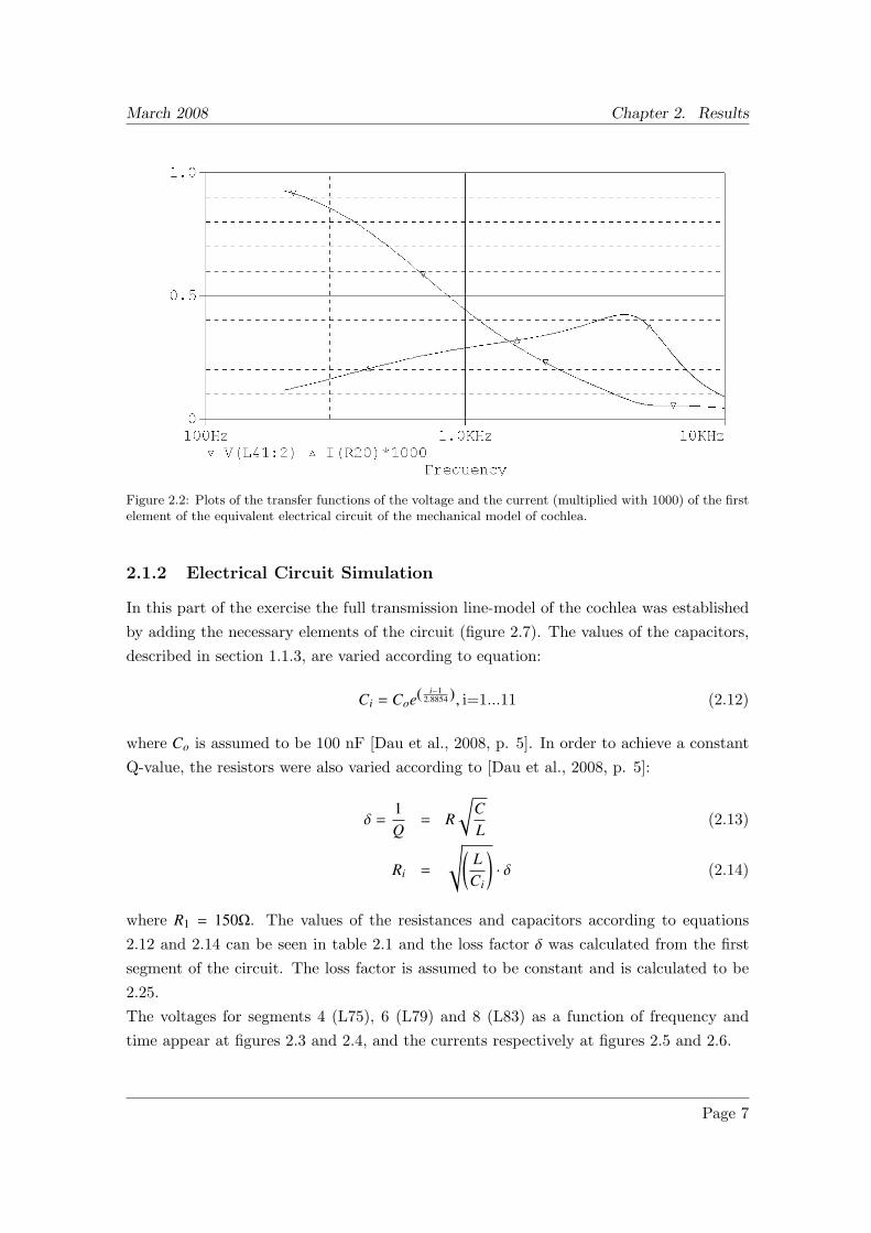
2.1.2 Electrical Circuit Simulation

In this part of the exercise the full transmission line-model of the cochlea was establishedby adding the necessary elements of the circuit (figure 2.7). The values of the capacitors,described in section 1.1.3, are varied according to equation:

Ci = Coe( i−12.8854 ), i=1...11 (2.12)

where Co is assumed to be 100 nF [Dau et al., 2008, p. 5]. In order to achieve a constantQ-value, the resistors were also varied according to [Dau et al., 2008, p. 5]:

δ =1Q

= R

√CL

(2.13)

Ri =

√(LCi

)· δ (2.14)

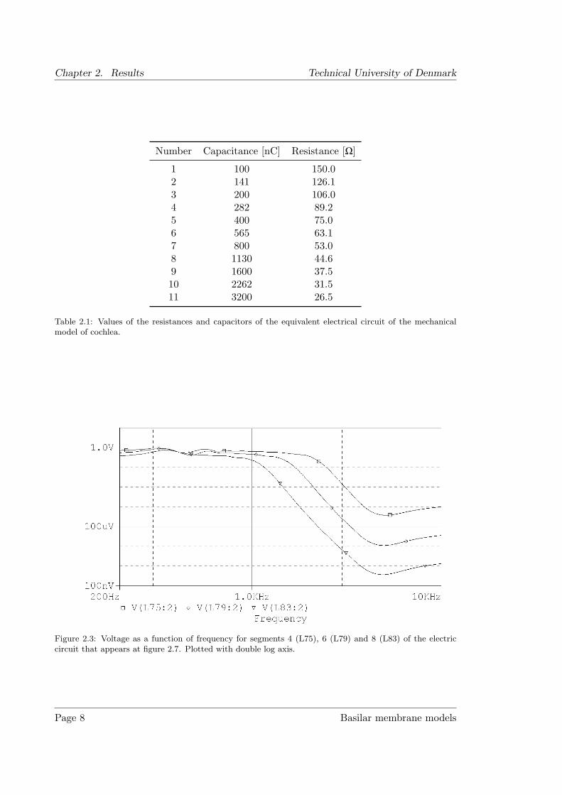
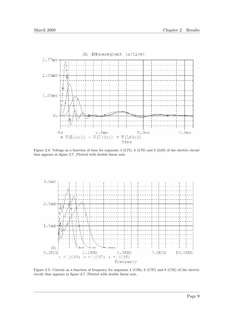
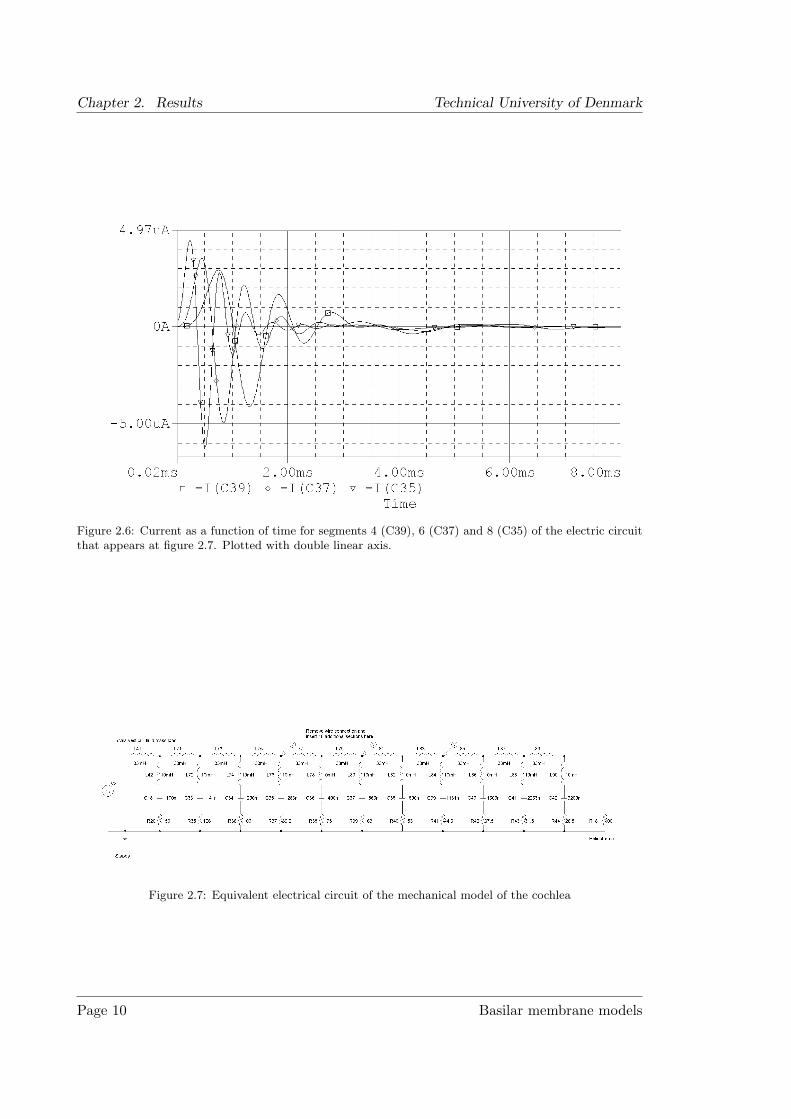
where R1 = 150Ω. The values of the resistances and capacitors according to equations2.12 and 2.14 can be seen in table 2.1 and the loss factor δ was calculated from the firstsegment of the circuit. The loss factor is assumed to be constant and is calculated to be2.25.The voltages for segments 4 (L75), 6 (L79) and 8 (L83) as a function of frequency andtime appear at figures 2.3 and 2.4, and the currents respectively at figures 2.5 and 2.6.

Page 7


Number Capacitance [nC] Resistance [Ω]

1 100 150.02 141 126.13 200 106.04 282 89.25 400 75.06 565 63.17 800 53.08 1130 44.69 1600 37.510 2262 31.511 3200 26.5

Table 2.1: Values of the resistances and capacitors of the equivalent electrical circuit of the mechanicalmodel of cochlea.

Figure 2.3: Voltage as a function of frequency for segments 4 (L75), 6 (L79) and 8 (L83) of the electriccircuit that appears at figure 2.7. Plotted with double log axis.



Figure 2.4: Voltage as a function of time for segments 4 (L75), 6 (L79) and 8 (L83) of the electric circuitthat appears at figure 2.7. Plotted with double linear axis.

Figure 2.5: Current as a function of frequency for segments 4 (C39), 6 (C37) and 8 (C35) of the electriccircuit that appears at figure 2.7. Plotted with double linear axis.

Page 9


Figure 2.6: Current as a function of time for segments 4 (C39), 6 (C37) and 8 (C35) of the electric circuitthat appears at figure 2.7. Plotted with double linear axis.

Figure 2.7: Equivalent electrical circuit of the mechanical model of the cochlea



2.2 Gammatone-filter model

2.2.1 Analysis of a single gammatone filter

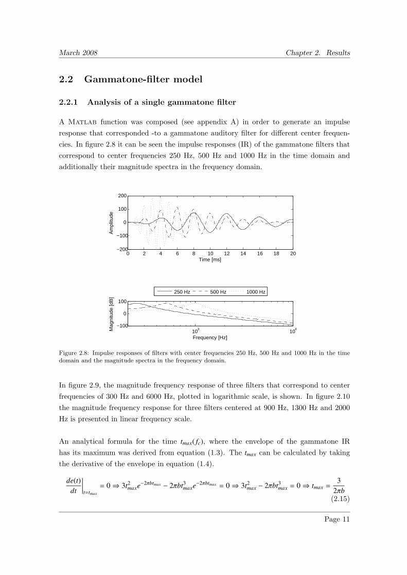
A Matlab function was composed (see appendix A) in order to generate an impulseresponse that corresponded -to a gammatone auditory filter for different center frequen-cies. In figure 2.8 it can be seen the impulse responses (IR) of the gammatone filters thatcorrespond to center frequencies 250 Hz, 500 Hz and 1000 Hz in the time domain andadditionally their magnitude spectra in the frequency domain.

0 2 4 6 8 10 12 14 16 18 20−200

−100

0

100

200

Am

plitu

de

Time [ms]

103

104

−100

0

100

Mag

nitu

de [d

B]

Frequency [Hz]

250 Hz 500 Hz 1000 Hz

Figure 2.8: Impulse responses of filters with center frequencies 250 Hz, 500 Hz and 1000 Hz in the timedomain and the magnitude spectra in the frequency domain.

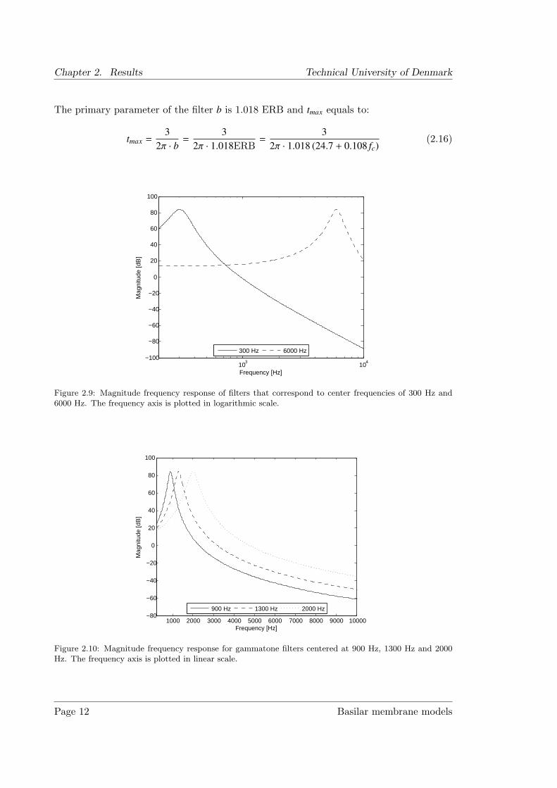
In figure 2.9, the magnitude frequency response of three filters that correspond to centerfrequencies of 300 Hz and 6000 Hz, plotted in logarithmic scale, is shown. In figure 2.10the magnitude frequency response for three filters centered at 900 Hz, 1300 Hz and 2000Hz is presented in linear frequency scale.

An analytical formula for the time tmax( fc), where the envelope of the gammatone IRhas its maximum was derived from equation (1.3). The tmax can be calculated by takingthe derivative of the envelope in equation (1.4).

de(t)dt

∣∣∣∣∣t=tmax

= 0⇒ 3t2maxe−2πbtmax − 2πbt3

maxe−2πbtmax = 0⇒ 3t2max − 2πbt3

max = 0⇒ tmax =3

2πb(2.15)

Page 11


The primary parameter of the filter b is 1.018 ERB and tmax equals to:

tmax =3

2π · b=

32π · 1.018ERB

=3

2π · 1.018 (24.7 + 0.108 fc)(2.16)

103

104

−100

−80

−60

−40

−20

0

20

40

60

80

100

Mag

nitu

de [d

B]

Frequency [Hz]

300 Hz 6000 Hz

Figure 2.9: Magnitude frequency response of filters that correspond to center frequencies of 300 Hz and6000 Hz. The frequency axis is plotted in logarithmic scale.

1000 2000 3000 4000 5000 6000 7000 8000 9000 10000−80

−60

−40

−20

0

20

40

60

80

100

Mag

nitu

de [d

B]

Frequency [Hz]

900 Hz 1300 Hz 2000 Hz

Figure 2.10: Magnitude frequency response for gammatone filters centered at 900 Hz, 1300 Hz and 2000Hz. The frequency axis is plotted in linear scale.



2.2.2 Analysis of the gammatone auditory filterbank

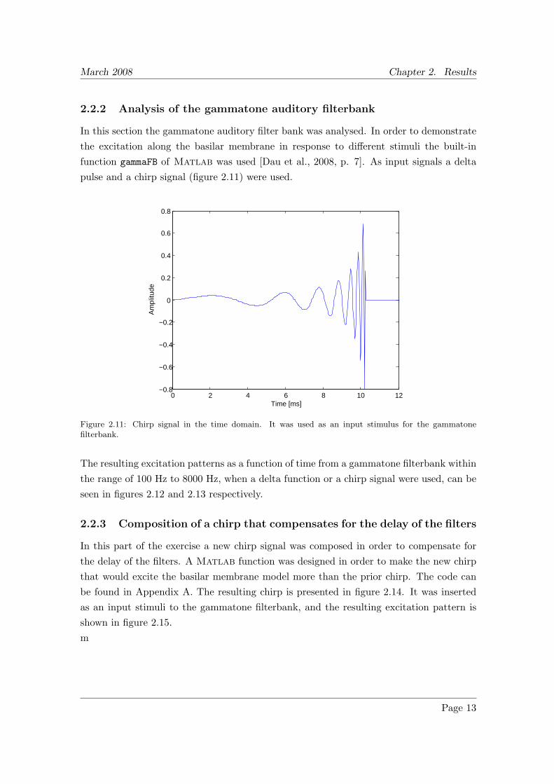
In this section the gammatone auditory filter bank was analysed. In order to demonstratethe excitation along the basilar membrane in response to different stimuli the built-infunction gammaFB of Matlab was used [Dau et al., 2008, p. 7]. As input signals a deltapulse and a chirp signal (figure 2.11) were used.

0 2 4 6 8 10 12−0.8

−0.6

−0.4

−0.2

0

0.2

0.4

0.6

0.8

Time [ms]

Am

plitu

de

Figure 2.11: Chirp signal in the time domain. It was used as an input stimulus for the gammatonefilterbank.

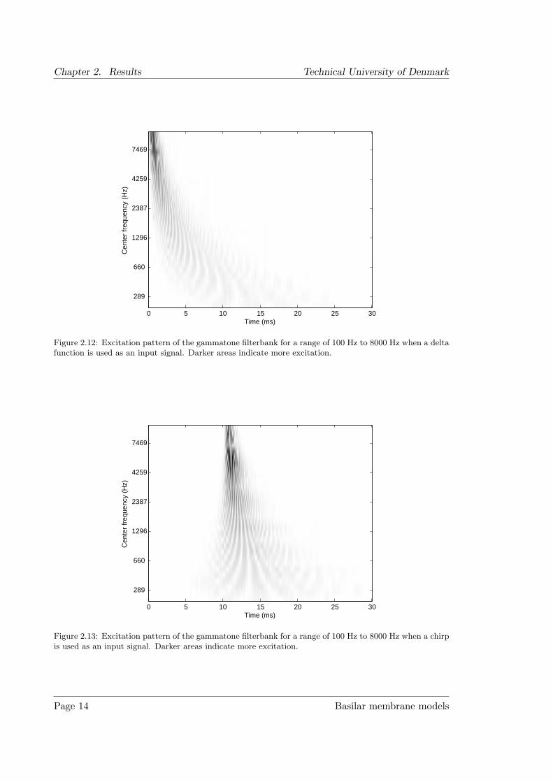
The resulting excitation patterns as a function of time from a gammatone filterbank withinthe range of 100 Hz to 8000 Hz, when a delta function or a chirp signal were used, can beseen in figures 2.12 and 2.13 respectively.

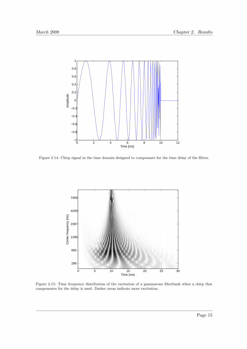
2.2.3 Composition of a chirp that compensates for the delay of the filters

In this part of the exercise a new chirp signal was composed in order to compensate forthe delay of the filters. A Matlab function was designed in order to make the new chirpthat would excite the basilar membrane model more than the prior chirp. The code canbe found in Appendix A. The resulting chirp is presented in figure 2.14. It was insertedas an input stimuli to the gammatone filterbank, and the resulting excitation pattern isshown in figure 2.15.m

Page 13


Time (ms)

Cen

ter

freq

uenc

y (H

z)

0 5 10 15 20 25 30

289

660

1296

2387

4259

7469

Figure 2.12: Excitation pattern of the gammatone filterbank for a range of 100 Hz to 8000 Hz when a deltafunction is used as an input signal. Darker areas indicate more excitation.

Time (ms)

Cen

ter

freq

uenc

y (H

z)

0 5 10 15 20 25 30

289

660

1296

2387

4259

7469

Figure 2.13: Excitation pattern of the gammatone filterbank for a range of 100 Hz to 8000 Hz when a chirpis used as an input signal. Darker areas indicate more excitation.



0 2 4 6 8 10 12−1

−0.8

−0.6

−0.4

−0.2

0

0.2

0.4

0.6

0.8

1

Time [ms]

Am

plitu

de

Figure 2.14: Chirp signal in the time domain designed to compensate for the time delay of the filters.

Time (ms)

Cen

ter

freq

uenc

y (H

z)

0 5 10 15 20 25 30

289

660

1296

2387

4259

7469

Figure 2.15: Time frequency distribution of the excitation of a gammatone filterbank when a chirp thatcompensates for the delay is used. Darker areas indicate more excitation.

Page 15

March 2008 Chapter 3. Discussion

Chapter 3Discussion


The two models of the basilar membrane are based on different approaches in theirpremises. The transmission line model is based on the mechanical properties of the basilarmembrane and implemented taking advantage of the electro-mechanical analogies. Thedesigned circuit has several segments or filters, modeling areas of the basilar membranewith different impedances. The changes on the values of R and C, equivalent to the damp-ing and the compliance, result in different center frequencies of these filters. A singlesegment of the model is analyzed and the resulting transfer functions for the voltage andcurrent (or force and velocity) are shown in figure 2.2. The force presents a low-pass filtercharacteristics, showing that no further segments will be highly excited with the highestfrequencies. When several segments are connected in cascade, the output of each one isthe input for the next, and it is possible to see that at each output, the frequency rangeis reduced. This shows that the lowest frequencies travel longer distance along the basilarmembrane.

The current observed at figure 2.2 presents a band-pass filter characteristics and this isequivalent to say that the velocity of a segment on the basilar membrane has a maximumamplitude which depends on the stimulus frequency and that there is one particular areaat the basilar membrane that responds maximally for each given frequency.

By analyzing different segments on the circuit (see figures 2.5 and 2.6), it can be seenthat the maximum amplitude of the current impulse response (or velocity of the basilarmembrane segments) is delayed inversely proportional to the center frequency of the filter.From the first figure, it can also be seen that the slope towards low frequencies of each filter

Page 17

Chapter 3. Discussion Technical University of Denmark

is steeper than the slope towards high frequencies. This proves that the upward spread ofmasking is related to the mechanical properties of the basilar membrane. It should alsobe noticed in figure 2.3 that the cut-off frequency of the low-pass filters becomes lowerat the latter segments of the circuit, so the excitations for the latest segments lack ofhigh-frequency content (only low-frequencies propagate).

3.2 Gammatone filterbank model

The gammatone filterbank is designed to be more efficient and faster in computationalterms than the transmission-line model. This model is able to take into account thedelays at the different parts of the basilar membrane as well as the associated tuning fre-quencies, as it is shown in figure 2.8. As it happened with the transmission-line model,the filters with lower center frequencies present higher delay at the maximum position ofthe impulse response, given by equation (2.16). At the same time, the filters with highcenter frequencies have a shorter overall duration in comparison to the ones with lower cen-ter frequencies. The frequency response of these filters is symmetric in a linear frequencyscale and not in a logarithmic one, as it can be observed by comparing figures 2.9 and 2.10.

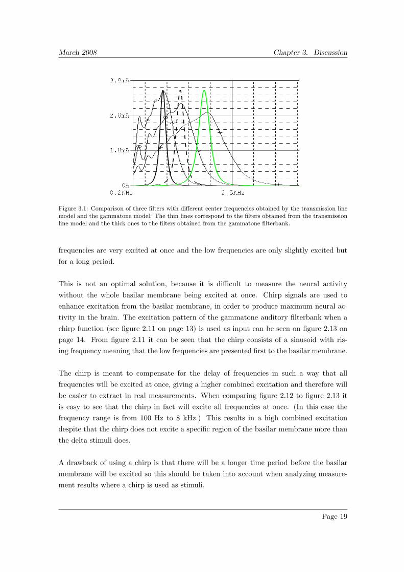
In figure 3.1, the responses of three filters obtained by the transmission line model and thegammatone filterbank are compared. It can be observed that the gammatone filters aremuch narrower, but despite this fact, the slopes at the both sides of the center frequencyappear to be equally steep, in opposition to the transmission-line model. The peaks in thefrequency responses of the gammatone filters are equal amongst them, because they havebeen calculated as independent filters, whereas the transmission-line filters represent theresult of a cascade system.

3.3 Excitation patterns

The excitation pattern of the gammatone auditory filterbank when a delta function is usedas input can be seen on figure 2.12 on page 14. It can be seen that the delta pulse excitesthe basilar membrane almost instantaneously and degrades fast. It is clearly seen thatthe high frequencies are excited far more than the low frequencies which have a longertraveling time and will therefore be excited at a later time. E.g. frequencies above 1 kHzare excited within 1 ms and frequencies below 300 Hz are first excited after 5 ms.

The reason for the high frequencies being excited far more than the low frequencies isbecause the high frequencies are excited in a short time period, and the low frequenciesare excited for a much longer period but with the same energy. This means that the high


March 2008 Chapter 3. Discussion

Figure 3.1: Comparison of three filters with different center frequencies obtained by the transmission linemodel and the gammatone model. The thin lines correspond to the filters obtained from the transmissionline model and the thick ones to the filters obtained from the gammatone filterbank.

frequencies are very excited at once and the low frequencies are only slightly excited butfor a long period.

This is not an optimal solution, because it is difficult to measure the neural activitywithout the whole basilar membrane being excited at once. Chirp signals are used toenhance excitation from the basilar membrane, in order to produce maximum neural ac-tivity in the brain. The excitation pattern of the gammatone auditory filterbank when achirp function (see figure 2.11 on page 13) is used as input can be seen on figure 2.13 onpage 14. From figure 2.11 it can be seen that the chirp consists of a sinusoid with ris-ing frequency meaning that the low frequencies are presented first to the basilar membrane.

The chirp is meant to compensate for the delay of frequencies in such a way that allfrequencies will be excited at once, giving a higher combined excitation and therefore willbe easier to extract in real measurements. When comparing figure 2.12 to figure 2.13 itis easy to see that the chirp in fact will excite all frequencies at once. (In this case thefrequency range is from 100 Hz to 8 kHz.) This results in a high combined excitationdespite that the chirp does not excite a specific region of the basilar membrane more thanthe delta stimuli does.

A drawback of using a chirp is that there will be a longer time period before the basilarmembrane will be excited so this should be taken into account when analyzing measure-ment results where a chirp is used as stimuli.

Page 19

Chapter 3. Discussion Technical University of Denmark

From figure 2.13 it can be seen that despite using a chirp and exciting all frequenciesat once, each filter in the model is not maximum excited at the same time. The highfrequencies have maximum excitation around 11 ms whereas the low frequencies havemaximum excitation around 14 ms - 15 ms. To solve this, a new chirp is developed usingknowledge of the model. This means that the new chirp is developed specifically for thegammatone filterbank model. Figure 2.14 on page 15 shows the chirp in time domain andthe excitation pattern can be seen on figure 2.15 on page 15.

Now all frequencies have maximum excitation at once (around 10 ms). It is also clearlyseen that the model predicts much higher excitation of the basilar membrane for eachfilter.


March 2008 Chapter 4. Conclusion

Chapter 4Conclusion

Two basilar membrane models are investigated in this report. The models are implementedusing Pspice and Matlab. Both methods assume linearity in the basilar membrane trans-fer function.

It is possible to model the basilar membrane, just by taking into account its mechani-cal properties: mass, compliance and damping. This model is called the transmission-linemodel and it can be implemented by using electric components, taking advantage of theelectro-mechanical analogies, where mass is represented by inductors, compliance by ca-pacitors and damping by resistances. The voltage of the electrical circuit corresponds toforce and the current to velocity.

Another approach based on the gammatone filterbank model offers a range of independentfilters that describe the shape of the impulse response function of the auditory system fordifferent inputs.

When both models are compared, the transmission line model seems more realistic thanthe gammatone filterbank, because it explains several effects that take place in the basilarmembrane, such as the upward spread of masking and the traveling wave (or distributionof the frequencies along the cochlea), assuming that the basilar membrane behaves in alinear way. However, it requires a considerable computational load and it is not suitablefor real-time analysis of signals, where the gammatone filterbank model is preferred.

To maximize the excitation from the basilar membrane, a chirp stimuli is better thana delta impulse. This is because the chirp is designed to stimulate all frequencies onthe basilar membrane at once, compensating for the non-homogeneous delay of different

Page 21

Chapter 4. Conclusion Technical University of Denmark

frequency components of a signal.


March 2008 Bibliography

Bibliography

[Dau, 2008] Dau, T. (2008). Cochlear transformation. Slide show.

[Dau et al., 2008] Dau, T., Favrot, S., and Jepsen, M. L. (2008). Exercise 3: Basilarmembrane models. 2.0.1 edition.

[de Boer, 1980] de Boer, E. (1980). Auditory Physics. Physical principles in hearing theoryI.

Page 23

Bibliography Technical University of Denmark


Project group 5 March 2008

Appendix AMatlab Code

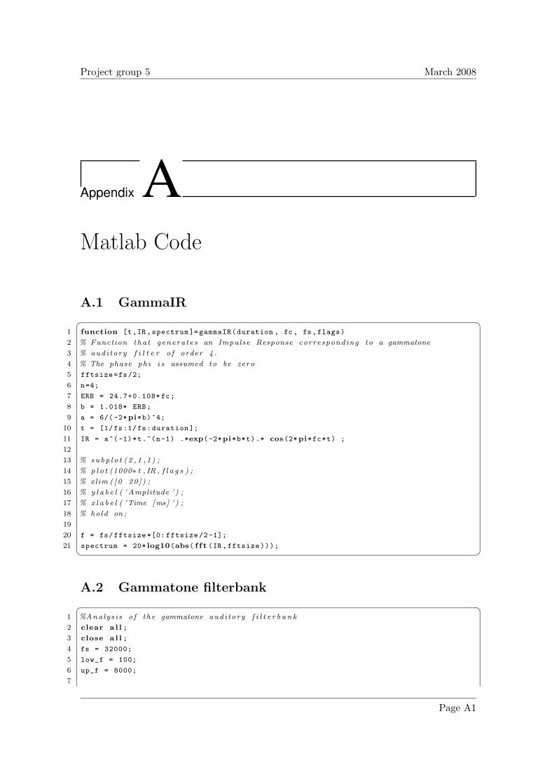
A.1 GammaIR 1 function [t,IR,spectrum ]= gammaIR(duration , fc, fs,flags)

2 % Function tha t genera tes an Impulse Response corresponding to a gammatone

3 % audi tory f i l t e r o f order 4 .

4 % The phase phi i s assumed to be zero

5 fftsize=fs/2;

6 n=4;

7 ERB = 24.7+0.108* fc;

8 b = 1.018* ERB;

9 a = 6/(-2*pi*b)^4;

10 t = [1/fs:1/fs:duration ];

11 IR = a^(-1)*t.^(n-1) .*exp(-2*pi*b*t).* cos(2*pi*fc*t) ;

12

13 % subp l o t (2 ,1 ,1) ;

14 % p l o t (1000∗ t , IR , f l a g s ) ;

15 % xlim ( [ 0 20 ] ) ;

16 % y l a b e l ( ’ Amplitude ’ ) ;

17 % x l a b e l ( ’Time [ms ] ’ ) ;

18 % hold on ;

19

20 f = fs/fftsize *[0: fftsize /2-1];

21 spectrum = 20* log10(abs( f f t (IR,fftsize))); A.2 Gammatone filterbank

1 %Analys i s o f the gammatone aud i tory f i l t e r b a n k

2 clear a l l ;

3 close a l l ;

4 fs = 32000;

5 low_f = 100;

6 up_f = 8000;

7

Page A1

APPENDIX

8 % 3.2

9 duration = fs * 125e-3;

10 chirp = genBMchirp(low_f ,up_f ,fs);

11 delta = dPulse(duration ,1);

12 [out ,cfs] = gammaFB(delta ,low_f ,up_f ,fs);

13 timeFreqDistribution(out , cfs , fs, [0 30])

14 [out ,cfs] = gammaFB(chirp ,low_f ,up_f ,fs);

15 timeFreqDistribution(out , cfs , fs, [0 30])

16

17 figure ;

18 t = [1/fs:1/fs:125e-3];

19 plot(t*1000, chirp);

20 xlim ([0 12]);

21 xlabel(’Time [ms]’);

22 ylabel(’Amplitude ’);

23

24 % Optional

25 figure ;

26 tdur =10e-3; % durat ion o f the ch i rp (10 ms l i k e the prev ious one )

27 t = [1/fs:1/fs:125e-3]; % time vec tor

28 int_matrix = triu (ones( length(t), length(t))); % Matrix in order to c a l c u l a t e the

i n t e g r a l

29 f = min((1/0.108) *(3./(1.018*2*pi*(tdur -t)) -24.7) ,20000); % Calcu la t i on o f f ( t )

30 phase = 2*pi*(f*int_matrix)*1/fs; % Calcu la t i on o f phase

31 chirp_opt = sin(phase); % Calcu la t i on o f op t i ona l ch i rp

32 chirp_opt(tdur*fs: length(chirp_opt))=0; % Zero−padding a f t e r 10 ms

33 [out ,cfs] = gammaFB(chirp_opt ,low_f ,up_f ,fs);

34 timeFreqDistribution(out , cfs , fs, [0 30]) %Plot the TimeFrequencyDistr ibut ion A.3 Chirp that compensates for the delay of the flters

1 close a l l ;

2 clear a l l ;

3

4 fs =32000;

5 tdur =10e-3;

6

7 t = [1/fs:1/fs:125e-3];

8 int_matrix = triu (ones( length(t), length(t)));

9 f = min((1/0.108) *(3./(1.018*2*pi*(tdur -t)) -24.7) ,20000);

10 phase = 2*pi*(f*int_matrix)*1/fs;

11 chirp2 = sin(phase);

12 chirp2(tdur*fs: length(chirp2))=0;

13 % p l o t ( t ∗1000 , ch irp2 ) ;

14 % xlim ( [ 0 tdur ∗1000]) ;

Page A2 Basilar membrane models

technical university of denmark - troels...

Documents