Contents lists available at SciVerse ScienceDirect

Journal of Financial Economics

Journal of Financial Economics 106 (2012) 132–156

0304-40

http://d

$ We

anonym

seminar

Institut

Univers

2009 Co

Copenh

and the

Retirem

Economn Corr

E-m

journal homepage: www.elsevier.com/locate/jfec

Testing conditional factor models$

Andrew Ang a,b, Dennis Kristensen c,d,n

a Columbia University, United Statesb NBER, United Statesc UCL, United Kingdomd IFS, United Kingdom

a r t i c l e i n f o

Article history:

Received 20 April 2009

Received in revised form

30 September 2011

Accepted 25 October 2011Available online 21 April 2012

JEL classifications:

C12

C13

C14

C32

G12

Keywords:

Nonparametric estimator

Time-varying beta

Conditional alpha

Book-to-market premium

Value and momentum

5X/$ - see front matter & 2012 Elsevier B.V.

x.doi.org/10.1016/j.jfineco.2012.04.008

thank Pengcheng Wan for research assistan

ous referees, Matias Cattaneo, Will Goetzma

participants at Columbia University, Dartm

e of Technology, Oxford-Man Institute of Q

ity in St. Louis, Yale University, University of

nference on ‘‘Semiparametric and Nonparam

agen 2009 Conference on ‘‘Recent Developme

New York University Five Star 2009 confe

ent (Netspar). Dennis Kristensen acknowledg

etric Analysis of Time Series (CREATES) and

esponding author at: UCL, United Kingdom.

ail addresses: aa610@columbia.edu (A. Ang),

a b s t r a c t

Using nonparametric techniques, we develop a methodology for estimating and testing

conditional alphas and betas and long-run alphas and betas, which are the averages of

conditional alphas and betas, respectively, across time. The estimators and tests can be

implemented for a single asset or jointly across portfolios. The traditional Gibbons, Ross,

and Shanken (1989) test arises as a special case of no time variation in the alphas and

factor loadings and homoskedasticity. As applications of the methodology, we estimate

conditional CAPM and multifactor models on book-to-market and momentum decile

portfolios. We reject the null that long-run alphas are equal to zero even though there is

substantial variation in the conditional factor loadings of these portfolios.

& 2012 Elsevier B.V. All rights reserved.

1. Introduction

Under the null of a factor model, an asset’s expectedexcess return should be zero after controlling for that asset’ssystematic factor exposure. Traditional regression tests of

All rights reserved.

ce and Kenneth French

nn, Jonathan Lewellen,

outh University, Georget

uantitative Finance, Prin

Montreal, the American F

etric Methods in Econom

nts in Financial Econome

rence. Andrew Ang ackn

es funding from the Dani

the National Science Fou

d.kristensen@ucl.ac.uk (D

whether an alpha is equal to zero, such as the widely usedGibbons, Ross, and Shanken (1989) test, assume that thefactor loadings are constant. However, overwhelming empiri-cal evidence shows that factor loadings, especially for thestandard capital asset pricing model (CAPM) and Fama and

for providing data. For helpful comments and suggestions, we thank the

Serena Ng, Jay Shanken, Masahiro Watanabe and Guofu Zhou, as well as

own University, Emory University, Federal Reserve Board, Massachusetts

ceton University, State University in New York at Albany, Washington

inance Association 2010 meeting, the Banff International Research Station

etrics’’, the Econometric Society Australasian 2009 meeting, the Humboldt-

trics’’, the 2010 National Bureau of Economic Research Summer Institute,

owledges funding from the Network for Studies on Pension, Aging and

sh National Research Foundation through a grant to Center for Research in

ndation (grant no. SES-0961596).

. Kristensen).

2 The instrumental variables approach is taken by Shanken (1990)

A. Ang, D. Kristensen / Journal of Financial Economics 106 (2012) 132–156 133

French (1993) models, vary substantially over time. Factorloadings exhibit variation even at the portfolio level (see,among others, Fama and French, 1997; Lewellen and Nagel,2006; Ang and Chen, 2007). Time-varying factor loadings candistort standard factor model tests for whether the alphas areequal to zero and, thus, render traditional statistical inferencefor the validity of a factor model to be possibly misleading.

We introduce a methodology to estimate time-varyingalphas and betas in conditional factor models. Conditionalon the realized alphas and betas, our factor specificationcan be regarded as a regression model with changingregression coefficients. We impose no parametric assump-tions on the nature of the realized time variation of thealphas and betas and estimate them nonparametricallybased on techniques similar to those found in the literatureon realized volatility (see, e.g., Foster and Nelson, 1996;Andersen, Bollerselv, Diebold, and Wu, 2006).1 We alsodevelop estimators of the long-run alphas and betas,defined as the averages of the conditional alphas or factorloadings, respectively, across time. Our estimators arehighly robust due to their nonparametric nature.

Based on the conditional and long-run estimators, wepropose short- and long-run tests for the asset pricingmodel. Major advantages of our estimators and tests arethat they are straightforward to apply, powerful, and involveno more than running a series of kernel-weighted ordinaryleast-squares (OLS) regressions for each asset. The tests canbe applied to a single asset or jointly across a system ofassets. In the special case in which betas are constantand there is no heteroskedasticity, our long-run tests forwhether the long-run alphas equal zero are asymptoticallyequivalent to Gibbons, Ross, and Shanken (1989).

We analyze the estimators and tests in a continuous-timesetting where the conditional alphas and betas can bethought of as the instantaneous drift of the assets and thecovariance between asset and factor returns, respectively. Allour estimations, however, are of discrete-time models and soour methodology is widely applicable to the majority ofempirical asset studies that estimate factor models in discretetime. As is well known from the literature on drift andvolatility estimation in continuous time, one can learn aboutvolatilities or covariances from data for any fixed time spanwith increasingly dense observations, while pinning downthe drift requires a long span of data (see, e.g., Merton, 1980).We obtain similar results in our setting: The conditional betaestimators are consistent under very weak restrictions on thedata-generating process for fixed time spans, while theconditional alpha estimators are, in general, inconsistent.

Whereas a large number of applied papers implementrolling-window estimators of conditional alphas and use themin statistical inference (see the summary by Ferson and Qian,2004), under a continuous-time model we show that condi-tional alphas cannot be estimated consistently. However, we

1 Other papers in finance developing nonparametric estimators include

Stanton (1997), Aıt-Sahalia (1996), and Bandi (2002), who estimate drift and

diffusion functions of the short rate. Bansal and Viswanathan (1993),

Aıt-Sahalia and Lo (1998), and Wang (2003) characterize the pricing kernel

by nonparametric estimation. Brandt (1999) and Aıt-Sahalia and Brandt

(2007) present applications of nonparametric estimators to portfolio choice

and consumption problems.

demonstrate that under additional restrictions on the modelinvolving certain time normalizations of the model para-meters, a formal asymptotic theory of the conditional alphaestimators can, in fact, be developed. These additional assump-tions supply conditions under which the popular rolling-window conditional alphas have well-defined (asymptotic)distributions, but the required time normalization is econom-ically counterintuitive when interpreted in the context of acontinuous-time factor model. In contrast to the conditionalalphas, the long-run alphas are identified from data withoutany time normalizations. We develop an asymptotic theory forour long-run alpha and beta estimators, which converge atstandard rates as found in parametric diffusion models.

Our approach builds on a literature advocating the useof short windows with high-frequency data to estimatetime-varying second moments or betas, such as French,Schwert, and Stambaugh (1987) and Lewellen and Nagel(2006). In particular, Lewellen and Nagel estimate time-varying factor loadings and infer conditional alphas. In thesame spirit of Lewellen and Nagel, we use local informationto obtain estimates of conditional alphas and betas withouthaving to instrument time-varying factor loadings withmacroeconomic and firm-specific variables.2 Our workextends this literature in several important ways.

First, we provide a formal distribution theory for condi-tional and long-run estimators which the earlier literaturedid not provide. For example, the Lewellen and Nagel(2006) procedure identifies the time variation of condi-tional betas and provides period-by-period estimates ofconditional alphas on short, fixed windows equally weight-ing all observations in that window. We show this is aspecial case (a one-sided filter) of our general estimator andso our theoretical results apply. Lewellen and Nagel furthertest whether the average conditional alpha is equal to zerousing a Fama and MacBeth (1973) procedure. Because thisis nested as a special case of our methodology, we provideformal arguments for the validity of this procedure. We alsodevelop data-driven methods for choosing optimal windowwidths used in estimation.

Second, using kernel methods to estimate time-varyingbetas we are able to use all the data efficiently in theestimation of conditional alphas and betas at any particulartime. Naturally, our methodology allows for any validkernel and so nests the one-sided, equal-weighted filtersused by French, Schwert, and Stambaugh (1987), Andersen,Bollerselv, Diebold, and Wu (2006), Lewellen and Nagel(2006) and others, as special cases. All of these studies usetruncated, backward-looking windows to estimate secondmoments that have larger mean square errors (MSEs)compared with estimates based on two-sided kernels.3

and Ferson and Harvey (1991), among others. As Ghysels (1998) and

Harvey (2001) note, the estimates of the factor loadings obtained using

instrumental variables are very sensitive to the variables included in

the information set. Furthermore, many conditioning variables, especially

macro and accounting variables, are only available at coarse frequencies.3 Foster and Nelson (1996) derive optimal two-sided filters to

estimate time-varying covariance matrices for a general class of time

series models. Foster and Nelson’s exponentially declining weights can be

replicated by special choice kernel weights. An advantage of using a

nonparametric procedure is that we obtain efficient estimates of betas

A. Ang, D. Kristensen / Journal of Financial Economics 106 (2012) 132–156134

Third, we develop tests for the significance of conditionaland long-run alphas jointly across assets in the presence oftime-varying betas. Earlier work incorporating time-varyingfactor loadings restricts attention to only single assets,whereas our methodology can incorporate a large numberof assets. Our procedure can be viewed as the conditionalanalogue of Gibbons, Ross, and Shanken (1989), who jointlytest whether alphas are equal to zero across assets, wherewe now permit the alphas and betas to vary over time. Jointtests are useful for investigating whether a relation betweenconditional alphas and firm characteristics strongly existsacross many portfolios and have been extensively used byFama and French (1993) and many others.

Our work is most similar to tests of conditional factormodels contemporaneously examined by Li and Yang(2011). Li and Yang also use nonparametric methods toestimate conditional parameters and formulate a test sta-tistic based on average conditional alphas. However, theydo this in a discrete-time setting, do not investigate condi-tional or long-run betas, and do not develop tests ofconstancy of conditional alphas or betas. One importantissue is the bandwidth selection procedure, which requiresdifferent bandwidths for conditional or long-run estimates.Li and Yang do not provide an optimal bandwidth selectionprocedure. They also do not derive specification tests jointlyacross assets as in Gibbons, Ross, and Shanken (1989),which we nest as a special case, or present a completedistribution theory for their estimators.

The rest of this paper is organized as follows. Section 2lays out our empirical methodology. Section 3 discusses ourdata. In Sections 4 and 5 we investigate tests of conditionalCAPM and Fama and French models on the book-to-marketand momentum portfolios, respectively. Section 6 con-cludes. We relegate all technical proofs to the Appendix.

2. Statistical methodology

We present our conditional factor model and developnonparametric estimators and test statistics for the condi-tional alphas and betas.

4 The strict factor structure rules out leverage effects and other

nonlinear relations between asset and factor returns, which Boguth,

Carlson, Fisher, and Simutin (2011) argue could lead to additional biases

2.1. Conditional factor model

Let R¼ ðR1, . . . ,RMÞ0 denote a vector of excess returns

of M assets observed at n time points, 0ot1ot2o � � �otnoT , within a time span T40. We wish to explain thereturns through a set of J common tradeable factors, f ¼

ðf 1, . . . ,f JÞ0, which are observed at the same time points. We

assume the following conditional factor model explains thereturns of stock k (k¼ 1, . . . ,M) at time ti (i¼ 1, . . . ,n):

Rk,i ¼ akðtiÞþbkðtiÞ0f iþokkðtiÞzk,i, ð1Þ

where Rk,i and fi are the observed return and factorsrespectively at time ti. This can be rewritten in matrix

(footnote continued)

without having to specify a particular data generating process, whether

this is generalized autoregressive conditional heteroskedastic (GARCH)

model (see, for example, Bekaert and Wu, 2000) or a stochastic volatility

model (see, for example, Jostova and Philipov, 2005; Ang and Chen, 2007).

notation

Ri ¼ aðtiÞþbðtiÞ0f iþO

1=2ðtiÞzi, ð2Þ

where aðtÞ ¼ ða1ðtÞ, . . . ,aMðtÞÞ02 RM is the vector of condi-

tional alphas across stocks k¼ 1, . . . ,M and bðtÞ ¼ ðb1ðtÞ, . . . ,bMðtÞÞ

02 RJ�M is the corresponding matrix of conditional

betas. The alphas and betas can take on any sample path inthe data, subject to the (weak) restrictions in Appendix A,including nonstationary and discontinuous cases, andtime-varying dependence of conditional betas and factors.The vector zi ¼ ðz1,i, . . . ,zM,iÞ

02 RM contains the errors and

the covariance matrix OðtÞ ¼ ½o2jkðtÞ�j,k 2 R

M�M allows forboth heteroskedasticity and time-varying cross-sectionalcorrelations.

Letting F i ¼F fRj,f j,aðtjÞ,bðtjÞ : jr ig denote the filtrationup to time ti, we assume the error term satisfies

E½zi9F i� ¼ 0 and E½zizi09F i� ¼ IM , ð3Þ

where IM denotes the M-dimensional identity matrix. Eq. (3)is the identifying assumption of the model and rules outnonzero correlations between the factor and the errors. Thisorthogonality assumption is an extension of standard OLS,which specifies that errors and factors are orthogonal.4

Importantly, this condition does not rule out the alphas andbetas being correlated with the factors. That is, the condi-tional factor loadings can be random processes in their ownright and exhibit (potentially time-varying) dependence withthe factors. Thus, we allow for a rich set of dynamic tradingstrategies of the factor portfolios.

We are interested in time series estimates of therealized conditional alphas, aðtÞ, and the conditional factorloadings, bðtÞ, along with their standard errors. Under thenull of a factor model, the conditional alphas are equal tozero, or aðtÞ ¼ 0. As Jagannathan and Wang (1996) pointout, if the correlation of the factor loadings, bðtiÞ, withfactors, fi, is zero, then the unconditional pricing errors of aconditional factor model are mean zero and an uncondi-tional OLS methodology could be used to test the condi-tional factor model. When the betas are correlated with thefactors then the unconditional alpha reflects both the trueconditional alpha and the covariance between the betasand the factor (see Jagannathan and Wang, 1996; Lewellenand Nagel, 2006).

Given the realized alphas and betas, we define the long-run alphas and betas for asset k¼ 1, . . . ,M as

aLR,k � limn-1

1

n

Xn

i ¼ 1

akðtiÞ 2 R,

bLR,k � limn-1

1

n

Xn

i ¼ 1

bkðtiÞ 2 RJ : ð4Þ

in the estimators. We expect that our theoretical results are still applic-

able under weaker assumptions, but this requires specification of the

appropriate correlation structure between the alphas, betas, and error

terms. Appendix A details our technical assumptions and Appendix B

contains proofs. We leave these extensions to further research. Simulation

results show that our long-run alpha estimators perform well under mild

misspecification of modestly correlated betas and error terms.

A. Ang, D. Kristensen / Journal of Financial Economics 106 (2012) 132–156 135

We use the terminology ‘‘long run’’ (LR) to distinguishthe conditional alpha at a particular time, akðtÞ, from theconditional alpha averaged over the sample, aLR,k. Whenthe factors are correlated with the betas, the long-runalphas are potentially different from OLS alphas.

We test the hypothesis that the long-run alphas arejointly equal to zero across M assets

H0 : aLR,k ¼ 0, k¼ 1, . . . ,M: ð5Þ

In a setting with constant alphas and betas, Gibbons, Ross,and Shanken (1989) develop a test of the null H0. Ourmethodology can be considered the conditional version ofthe Gibbons, Ross and Shanken test when both conditionalalphas and betas potentially vary over time. In addition, wetest the stronger hypothesis of the conditional alphas beingzero at any given point in time,

H0,k : akðtÞ ¼ 0 for all t: ð6Þ

2.2. Conditional estimators

Our analysis of the model and estimators is doneconditional on the particular realization of alphas and betasthat generated data. That is, our analysis relies on thefollowing conditional relation between the observationsand the parameters of interest that holds under theorthogonality condition in Eq. (3):

½aðtiÞ,bðtiÞ0�0 ¼L�1

ðtiÞE½XiRi09F i�, Xi ¼ ð1,f i

0Þ0, ð7Þ

where LðtiÞ denotes the conditional second moment of theregressors

LðtiÞ � E½XiXi09F i�: ð8Þ

Eq. (7) identifies the particular realization of alphas andbetas that generated data.

The time variation in LðtÞ reflects potential correlationbetween factors and betas. If there is zero correlation (and thefactors are stationary), then LðtÞ ¼L is constant over time, butin general LðtÞ varies over time. One advantage of conductingthe analysis conditional on the sample is that we can tailor ourestimates of the particular realization of alphas and betas.

A natural way to estimate aðtÞ and bðtÞ is by replacingthe population moments in Eq. (7) by their sample ver-sions. Given observations of returns and factors, we pro-pose the following local least squares estimators of akðtÞ

and bkðtÞ for asset k in Eq. (1) at any time 0rtrT:

½akðtÞ,bkðtÞ0�0 ¼ arg min

ða,bÞ

Xn

i ¼ 1

KhkT ðti�tÞðRk,i�a�b0f iÞ

2, ð9Þ

where KhkT ðzÞ � Kðz=ðhkTÞÞ=ðhkTÞ with Kð�Þ being a kerneland hk40 a bandwidth. The optimal estimators solvingEq. (9) are simply kernel-weighted least squares

½akðtÞ,bkðtÞ0�0 ¼

Xn

i ¼ 1

KhkT ðti�tÞXiXi0

" #�1 Xn

i ¼ 1

KhkT ðti�tÞXiRk,i

" #:

ð10Þ

The proposed estimators are sample analogues to Eq. (7)giving weights to the individual observations according tohow close in time they are to the time point of interest, t.The shape of the kernel, K, determines how the differentobservations are weighted. For most of our empirical work

we choose the Gaussian density as kernel,

KðzÞ ¼1ffiffiffiffiffiffi2pp exp �

z2

2

� �,

but also examine one-sided and uniform kernels that havebeen used in the literature by Andersen, Bollerselv, Diebold,and Wu (2006) and Lewellen and Nagel (2006), amongothers. In common with other nonparametric estimationmethods, as long as the kernel is symmetric, the mostimportant choice is not so much the shape of the kernel asthe bandwidth, hk. The bandwidth, hk 2 ð0;1Þ, controls theproportion of data obtained in the sample span ½0,T� that isused in the computation of the estimated alphas and betas.A small bandwidth means only observations very close to t

are included in the estimation. The bandwidth controls thebias and variance of the estimator and it should, in general,be sample specific. In particular, as the sample size grows,the bandwidth should shrink toward zero at a suitable ratein order for any finite-sample biases and variances to vanish.We discuss the bandwidth choice in Section 2.8.

We run the kernel regression in Eq. (9) separately stockby stock for k¼ 1, . . . ,M. This is a generalization of theregular OLS estimators, which are also run stock by stock inthe Gibbons, Ross, and Shanken (1989) test. If the samebandwidth h is used for all stocks, our estimator of alphasand betas across all stocks take the simple form of aweighted multivariate OLS estimator,

½aðtÞ,bðtÞ0�0 ¼Xn

i ¼ 1

KhT ðti�tÞXiXi0

" #�1 Xn

i ¼ 1

KhT ðti�tÞXiRi

" #:

ð11Þ

In practice it is not advisable to use one commonbandwidth across all assets. We use different bandwidthsfor different stocks because the variation and curvature ofthe conditional alphas and betas could differ widely acrossstocks and each stock could have a different level ofheteroskedasticity. We show below that, for book-to-market and momentum test assets, the patterns of condi-tional alphas and betas are dissimilar across portfolios.Choosing stock-specific bandwidths allows us to better adjustthe estimators for these effects. However, to avoid cumber-some notation, we present the asymptotic results for theestimators aðtÞ and bðtÞ assuming one common bandwidth,h, across all stocks. The asymptotic results are identical in thecase with multiple bandwidths under the assumption thatthese all converge at the same rate as n-1.

2.3. Continuous-time factor model

For the theoretical analysis of the proposed estimators,we introduce a continuous-time version of the discrete-timefactor model. Suppose that the vector of log-prices of theM risky assets (in excess of the risk-free asset), sðtÞ ¼

log SðtÞ 2 RM , solve the stochastic differential equation

dsðtÞ ¼ aðtÞ dtþbðtÞ0 dFðtÞþS1=2ðtÞ dBðtÞ, ð12Þ

where FðtÞ are J factors and BðtÞ is a M-dimensionalBrownian motion. This is the ANOVA (analysis of variance)model considered in Andersen, Bollerselv, Diebold, and Wu(2006) and Mykland and Zhang (2006). Suppose we have

A. Ang, D. Kristensen / Journal of Financial Economics 106 (2012) 132–156136

observed sðtÞ and FðtÞ over the time span ½0,T� at n discretetime points, 0rt0ot1o � � �otnrT . We wish to estimatethe spot alphas, aðtÞ 2 RM , and betas, bðtÞ 2 RJ�M , which canbe interpreted as the realized instantaneous drift of s(t) and(co-)volatility of ðsðtÞ,FðtÞÞ, respectively. For simplicity, weassume that the observations are equidistant in time suchthat D� ti�ti�1 is constant; in particular, nD¼ T .

To facilitate the analysis of the estimators in thisdiffusion setting, we introduce a discretized version ofthe continuous-time model,

Dsi ¼ aðtiÞDþbðtiÞ0DFiþS

1=2ðtiÞ

ffiffiffiffiDp

zi, i¼ 1;2, . . . ,n, ð13Þ

where zi are independently and identically distributed(i.i.d.) with mean zero and covariance IM ,

Dsi ¼ sðtiÞ�sðti�1Þ and DFi ¼ FðtiÞ�Fðti�1Þ:

In the following we treat Eq. (13) as the true, data-generating model. The extension to treat (12) as the truemodel would require some extra effort to ensure that thediscretized version in Eq. (13) is an asymptotically validapproximation of Eq. (12). The analysis would involvecontrolling the various discretization biases that wouldneed to vanish sufficiently fast as D-0. This could be donealong the lines of Bandi and Phillips (2003) and Kristensen(2010), among others.

Defining

Ri �Dsi=D, f i �DFi=D, Ot �SðtÞ=D, ð14Þ

we can rewrite the discretized diffusion model in the formof Eq. (2). Natural estimators of aðtÞ and bðtÞ, therefore, takeon the same form as the discrete-time estimators in Eq. (11).

2.4. Conditional beta estimators

We now analyze the properties of our estimator bðtÞunder the assumption that the discretized version of thediffusion model (13) is the data-generating process. As iswell known in the literature on the estimation of diffusionmodels (see, e.g., Merton, 1980; Bandi and Phillips, 2003;Kristensen, 2010), we can consistently estimate the instan-taneous betas, bðtÞ, as D-0 under weak regularity condi-tions. In addition to Eq. (13), we assume that the factorssatisfy the discretized diffusion model

DFi ¼ mF ðtiÞDþL1=2FF ðtiÞ

ffiffiffiffiDp

ui, ð15Þ

where ui � i:i:dð0,IJÞ and mð�Þ and LFF ð�Þ are r times differ-entiable (possibly random) functions.

Under regularity conditions stated in Appendix A, thebias and variance of the estimator are

E½bðtÞ�CbðtÞþðhTÞ2bð2ÞðtÞ and

VarðbðtÞÞC1

nh� k2L�1

FF ðtÞ � SðtÞ,

where bð2ÞðtÞ denotes the second derivative of bðtÞ andk2 ¼

RK2ðzÞ dz (¼0.2821 for the normal kernel).5 These

expressions show the usual trade-off between bias and

5 We assume that t/bðtÞ is twice differentiable. This assumption

could be replaced by, for example, a Lipschitz condition, JbðsÞ�bðtÞJrCJs�tJl for some l40, in which case the bias component would change

and be of order OððhTÞlÞ.

variance for kernel regression estimators with h needing tobe chosen to balance the two. In particular, as hT-0 andnh-1, bðtÞ-

pbðtÞ. Letting h-0 at a suitable rate, the bias

term can be ignored and we obtain the following asymptoticresult:

Theorem 1. Assume that assumptions A.1–A.3 given in

Appendix A hold and the bandwidth is chosen such that

nh-1 and nT4h5-0. Then, for any t 2 ½0,T�,ffiffiffiffiffiffi

nhpfbðtÞ�bðtÞg �Nð0,k2L

�1FF ðtÞ �SðtÞÞ in large samples:

ð16Þ

Moreover, the conditional estimators are asymptotically inde-

pendent across any set of distinct time points.

This result is a multivariate extension of the asymptoticdistribution for kernel-based estimators of spot volatilitiesfound in Kristensen (2009, Theorem 1). Andersen, Bollerselv,Diebold, and Wu (2006) develop estimators of integratedfactor loadings,

R T0 bðsÞ ds, which implicitly ignore the varia-

tion of beta within each window. Our estimator is a localversion of the asymptotics for the integrated beta (see alsoFoster and Nelson, 1996). By choosing a flat kernel and thebandwidth, h40, to match the chosen time window, ourproposed estimators nest the realized beta estimators. But,while Andersen, Bollerselv, Diebold, and Wu (2006) developan asymptotic theory for a fixed window width, Theorem 1establishes results in which the time window shrinks withsample size. This allows us to recover the instantaneousconditional betas.

In Theorem 1, the rate of convergence of bðtÞ isffiffiffiffiffiffinhp

,which is slower than parametric estimators because h-0.This is common to all nonparametric estimators. Theasymptotic analysis and properties of the estimators areclosely related to the kernel-regression type estimators ofdiffusion models proposed in Bandi and Phillips (2003),Kanaya and Kristensen (2010), and Kristensen (2010). Bandiand Phillips (2003) focus on univariate Markov diffusionprocesses and use the lagged value of the observed processas kernel regressor, while Kanaya and Kristensen (2010)and Kristensen (2010) consider estimation of univariatestochastic volatility models. In contrast, we model time-inhomogenous, multivariate processes in which the obser-vation times, t1, . . . ,tn, are used as the kernel regressor.Because we only smooth over the univariate time variable t,increasing the number of regressors, J, or the number ofstocks, M, does not affect the performance of the estimator.

Estimators of the two terms appearing in the asymptoticvariance in Eq. (16) are obtained as

LFF ðtÞ ¼DPn

i ¼ 1 KhT ðti�tÞ f i�mF ðtiÞ� �

½f i�mF ðtiÞ�0Pn

i ¼ 1 KhT ðti�tÞ,

SðtÞ ¼DPn

i ¼ 1 KhT ðti�tÞeiei0Pn

i ¼ 1 KhT ðti�tÞ, ð17Þ

where ei ¼ Ri�aðtiÞ�bðtiÞ0f i are the residuals and mF ðtÞ is an

estimator of the instantaneous drift in the factors,

mF ðtÞ ¼

Pni ¼ 1 KhT ðti�tÞf iPn

i ¼ 1 KhT ðti�tÞ: ð18Þ

A. Ang, D. Kristensen / Journal of Financial Economics 106 (2012) 132–156 137

Due to the asymptotic independence across differentvalues of t, confidence bands over a given grid of timepoints can easily be computed.

2.5. Conditional alpha estimators

Unlike conditional betas, conditional alphas are notidentified in data without additional restrictions on thetime series variation and without increasing the data overlong time spans (T-1), which was first demonstrated byMerton (1980). Without further restrictions, the estimatorof aðtÞ satisfies

E½aðtÞ�CaðtÞþðThÞ2að2ÞðtÞ, VarðaðtÞÞC 1

Th� k2SðtÞ, ð19Þ

as D-0. Relative to bðtÞ, the bias of aðtÞ is of the sameorder but its variance vanishes slower, 1=ðThÞ versus 1=ðnhÞ.The slower rate of convergence of VarðaðtÞÞ is a well-knownfeature of nonparametric drift estimators in diffusionmodels, as in Bandi and Phillips (2003), and is due to thesmaller amount of information regarding the drift relativeto the volatility found in data.

Observe that the bias and variance of aðtÞ are perfectlybalanced. To remove the bias, we have to let Th-0, butwith this bandwidth choice the variance explodes. Thissimply mirrors the well-known fact that, in continuoustime, the local variation of observed returns is too noisy toextract information about the drift. As such, we cannotstate any formal results regarding the asymptotic distribu-tion of aðtÞ. However, informally, with h chosen smallenough such that the bias is negligible, we haveffiffiffiffiffiffi

ThpfaðtÞ�aðtÞg �Nð0,k2SðtÞÞ in large samples: ð20Þ

It should be stressed, though, that without furtherrestriction on the data-generating process, the conditionalalpha estimates can be interpreted only as noisy estimatesof the underlying conditional alpha process. In particular,the computation of standard errors and confidence bandsfor the conditional alphas based on Eq. (20) ignores the biascomponent which might be substantial. As such, standarderrors and confidence bands for conditional alphas shouldbe interpreted with caution.

A large empirical asset pricing literature interpretsconstant terms in OLS regressions estimated over differentsample periods as conditional alphas, at least since Gibbonsand Ferson (1985).6 Given the wide-spread use of condi-tional alpha estimators, it is of interest to provide condi-tions under which the statement in Eq. (20) is formally (i.e.,asymptotically) correct.

One such condition is to impose a recurrency restrictionused in the literature on nonparametric estimation ofdiffusion models. In particular, Bandi and Phillips (2003)assume that the instantaneous drift (in our case, the spotalpha) is a function of a recurrent process, say ZðtÞ that visitsany given point in its domain, say z, infinitely often. Thus,

6 See, among many others, Shanken (1990), Ferson and Schadt (1996),

Christopherson, Ferson, and Glassman (1998), and more recently

Mamaysky, Spiegel and Zhang (2008). Ferson and Qian (2004) provide a

summary of this large literature.

under recurrence, there is increasing local informationaround z that allows identification of the drift function atthis value. A similar idea in our setting is to assume thereexists functions a : ½0;1�/RM and S : ½0;1�/RM�M suchthat the processes aðtÞ and SðtÞ are generated by

aðtÞ ¼ aðt=TÞ and SðtÞ ¼ Sðt=TÞ: ð21Þ

Then, the spot alpha would become a function ofZðtÞ � t=T 2 ½0;1�; in particular, Zi � ZðtiÞ, i¼ 1, . . . ,n, can bethought of as i.i.d. draws from the uniform distribution on½0;1� with observations growing more and more dense in[0,1] as T-1. Thus, with this assumption, we wouldaccomplish the same increase in local information aboutaðtÞ around a given point t in each successive model asT-1. In contrast, the un-normalized time, ZðtÞ ¼ t, is not arecurrent process, and so without the restriction given inEq. (21), we would not be able to identify aðtÞ.

Under the time normalization assumption in Eq. (21),there is a sequence of models as the sample changes (T

increases), and this sequence of models is constructed sothat the asymptotic distribution of aðtÞ is well defined.While the time normalization is a widely used statisticaltool to construct valid asymptotic distributions, and is usedextensively in the large structural change literature, therestriction imposed in Eq. (21) is counterintuitive becausethe underlying economic structure changes as we sampleover larger time spans. The time normalization is neededonly to obtain formal asymptotic results for the conditionalalpha estimators and not necessary for the asymptoticanalysis of the conditional beta estimators (Theorem 1)or the long-run alpha and beta estimators developed insubsequent sections. As a consequence, we relegate theasymptotic theory for the conditional alpha estimatorsunder the time normalization in Eq. (21) to Appendix C.

Finally, it is worth noting that one could alternativelyanalyze the conditional alpha and beta estimators in adiscrete-time setting, where it is necessary to impose atime normalization. This approach is pursued in a previousworking paper version of this paper (Ang and Kristensen,2011) and in Kristensen (2011). The normalization issimilar to Eq. (21), but in a discrete-time setting thenormalization restriction has to be imposed on both thealphas and betas. This is due to the fact that, in contrast tothe continuous-time setting where OðtÞ ¼SðtÞ=

ffiffiffiffiDp

-1 aswe sample more frequently, the variance in the discrete-time model does not change as we collect more data overtime. This mirrors the fact that in discrete time we relyonly on long-span asymptotics, and so cannot nonparame-trically learn about the local variation of the conditionalalphas and betas without imposing some type of timenormalization. However, as demonstrated in Ang andKristensen (2011), estimators and finite-sample standarderrors obtained in a discrete-time and continuous-timesetting, respectively, are numerically identical. Thus, whilethe asymptotic theory is different, the empirical imple-mentation is the same. The fact that the estimators canboth be given a discrete-time and continuous-time inter-pretation is a convenient feature of the estimators becausethe vast majority of empirical studies are carried out in adiscrete-time setting.

A. Ang, D. Kristensen / Journal of Financial Economics 106 (2012) 132–156138

2.6. Long-run alphas and betas

To test the null of whether the long-run (LR) alphas areequal to zero [H0 in Eq. (5)], we construct estimators ofthe long-run alphas and betas in Eq. (4). A natural wayto estimate the long-run alphas and betas for stock k isto simply plug the pointwise kernel estimators into theexpressions found in Eq. (4)

aLR,k ¼1

n

Xn

i ¼ 1

akðtiÞ and bLR,k ¼1

n

Xn

i ¼ 1

bkðtiÞ:

Given that we can identify the conditional spot betas,we can also identify the LR betas, and so bLR,k is consistent.But more important, we can identify the LR alphas even ifwe cannot identify the instantaneous ones. In particular,without the time normalization given in Eq. (21), akðtÞ isan inconsistent estimator of akðtÞ, but aLR,k is a consistentestimator of aLR,k. Thus, we can consistently estimate thelong-run alphas without imposing the time-normalizationused in the theoretical analysis of the conditional alphas.The intuition behind this feature is that our estimator ofaLR,k involves additional averaging over time. This aver-aging reduces the overall sampling error of aLR,k andenables consistency as T-1.

Theorem 2 states the joint distribution of aLR ¼

ðaLR,1, . . . , aLR,MÞ02 RM and bLR ¼ ðbLR,1, . . . ,bLR,MÞ

02 RJ�M

Theorem 2. Assume that assumptions A.1–A.5 given in

Appendix Ahold. Then the long-run estimators satisfy as T-1

ffiffiffiTpðaLR�aLRÞ �Nð0,SLR,aaÞ,

ffiffiffinpðbLR�bLRÞ �Nð0,SLR,bbÞ, ð22Þ

in large samples, where

aLR ¼ limT-1

1

T

Z T

0aðtÞ dt� E½aðtÞ�,

bLR ¼ limT-1

1

T

Z T

0bðtÞ dt� E½bðtÞ�,

SLR,aa ¼ limT-1

1

T

Z T

0SðtÞ dt� E½SðtÞ�,

and

SLR,bb ¼ limT-1

1

T

Z T

0L�1

FF ðtÞ � SðtÞ dt� E½L�1FF ðtÞ �SðtÞ�:

The long-run estimators converge at standard para-metric rates

ffiffiffinp

andffiffiffiTp

, despite the fact that they arebased on preliminary estimators that converge at slower,nonparametric rates. That is, inference of the long-runalphas and betas involves the standard Central LimitTheorem (CLT) convergence properties even though thepoint estimates of the conditional alphas and betas con-verge at slower rates. Intuitively, this is due to the addi-tional smoothing taking place when we average over thepreliminary estimates in Eq. (10). This occurs in othersemiparametric estimators involving integrals of kernelestimators (see, for example, Newey and McFadden, 1994,Section 8; Powell, Stock, and Stoker, 1989).

Consistent estimators of the asymptotic variances areobtained by simply plugging the point estimates of LFF ðtÞ

and SðtÞ given in Eq. (17) into the sample versions of SLR,aaand SLR,bb

SLR,aa ¼1

n

Xn

i ¼ 1

SðtiÞ, SLR,bb ¼1

n

Xn

i ¼ 1

L�1

FF ðtÞ � SðtiÞ:

We can test H0 : aLR ¼ 0 by the following Wald-typestatistic:

WLR ¼ Ta0

LRS�1

LR,aaaLR � w2M in large samples, ð23Þ

as a direct consequence of Theorem 2. This is a conditionalanalogue of Gibbons, Ross, and Shanken (1989) and tests iflong-run alphas are jointly equal to zero across all k¼ 1, . . . ,Mportfolios. A special case of Theorem 2 is Lewellen and Nagel(2006), who use a uniform kernel and the Fama and MacBeth(1973) procedure to compute standard errors of long-runestimators. Theorem 2 formally validates these procedures,and extend them to allow for general kernels, and joint testsacross stocks, and tests for long-run betas.

Our model includes the case in which the factor loadingsare constant with bðtÞ ¼ b 2 RJ�M for all t. Under the null thatthe beta’s are constant, bðtÞ ¼ b, and with no heteroskedas-ticity, SðtÞ ¼S for all t, the asymptotic distribution of aLR isidentical to the standard Gibbons, Ross, and Shanken (1989)test. This is shown in Appendix D. Thus, we pay no priceasymptotically for the added robustness of our estimator.Furthermore, only in a setting where the factors are uncorre-lated with the betas is the Gibbons, Ross and Shankenestimator of aLR consistent. This is not surprising given theresults of Jagannathan and Wang (1996) and others whoshow that in the presence of time-varying betas, OLS alphasdo not yield estimates of conditional or long-run alphas.

2.7. Tests for constancy of alphas and betas

We wish to test for constancy of the potentially time-varying conditional alphas and betas. The two null hypoth-eses of interest are formally

HkðaÞ : akðtÞ ¼ ak 2 R for all t 2 ½0,T�,

HkðbÞ : bkðtÞ ¼ bk 2 RJ for all t 2 ½0,T�: ð24Þ

We propose to test each of the two hypotheses throughHausman-type statistics where we compare two estima-tors. The first is chosen to be consistent both under therelevant null and the alternative while the second one isconsistent only under the null. If the null is true, the teststatistic is expected to be small and vice versa. A naturalchoice for the former estimator is the nonparametricestimator developed in Section 2.2. For the latter, we usethe long-run estimator because under the relevant null thelong-run estimator is a consistent estimator of the constantcoefficient. To be more precise, we define our test statisticsfor HkðaÞ and HkðbÞ, respectively, as the following twoweighted least-squares statistics:

WkðaÞ �1

n

Xn

i ¼ 1

s�2kk ðtiÞ½akðtiÞ�aLR,k�

2,

and

WkðbÞ �1

n

Xn

i ¼ 1

s�2kk ðtiÞ½bkðtiÞ�bLR,k�

0LFFðtiÞ½bkðtiÞ�bLR,k�: ð25Þ

7 For very finely sampled data, especially intra day data, nonsynchro-

nous trading could induce bias. A large literature exists on methods to

handle nonsynchronous trading going back to Scholes and Williams

(1977) and Dimson (1979). These methods can be employed in our

setting. As an example, consider the one-factor model in which f t ¼ Rm,t

is the market return. As an ad hoc adjustment for nonsynchronous

trading, we can augment the one-factor regression to include the lagged

market return, Rt ¼ atþb1,tRm,tþb2,tRm,t�1þet , and add the combined

betas, b t ¼ b1,tþ b2,t . This is done by Li and Yang (2011). More recently,

a literature has been growing on how to adjust for nonsynchronous effects

in the estimation of realized volatility. Again, these can

be carried over to our setting. For example, the methods proposed in,

for example, Hayashi and Yoshida (2005) or Barndorff-Nielsen, Hansen,

Lunde, and Shephard (2009) can be adapted to our setting to adjust for

biases due to nonsynchronous observations. In our empirical work,

nonsynchronous trading should not be a major issue as we work with

value-weighted, not equal-weighted, portfolios at the daily frequency.

A. Ang, D. Kristensen / Journal of Financial Economics 106 (2012) 132–156 139

The weights have been chosen to ensure that the asymp-totic distributions of the statistics are nuisance parameter-free. The two proposed test statistic are related to thegeneralized likelihood-ratio test statistics advocated in Fan,Zhang, and Zhang (2001).

The test statistic WkðaÞ depends on akðtÞ, which is ingeneral an inconsistent estimator of akðtÞ as discussed inSection 2.6. However, under the null of constant alphas,E½akðtÞ�CakðtÞ [c.f. Eq. (19)], and we are, therefore, ableto derive a formal large-sample distribution of WkðaÞ. Animportant hypothesis nested within HkðaÞ is the asset pricinghypothesis that ak,t ¼ 0 for all t 2 ½0,T� [H0,k in Eq. (6)]. Thiscan be tested by simply setting aLR,k ¼ 0 in WkðaÞ yielding:

Wkð0Þ �1

n

Xn

i ¼ 1

s�2kk ðtiÞa

2k ðtiÞ: ð26Þ

The proposed test statistics follow normal distributionsin large samples as stated in Theorem 3.

Theorem 3. Assume that assumptions A.1–A.5 given in

Appendix A hold and the bandwidth satisfies A.6. Then,

Under HkðaÞ :WkðaÞ�mðaÞ

vðaÞ �Nð0;1Þ,

Under HkðbÞ :WkðbÞ�mðbÞ

vðbÞ�Nð0;1Þ, ð27Þ

in large samples, where, with ðKnKÞðzÞ �R

KðyÞKðzþyÞ dy and

J¼ dimðf iÞ,

mðaÞ ¼ k2

Thand v2ðaÞ ¼

2RðKnKÞ2ðzÞ dz

T3h,

mðbÞ ¼k2JD

Thand v2ðbÞ ¼

2JRðKnKÞ2ðzÞ dz

n2Th:

For Gaussian kernels,RðKnKÞ2ðzÞ dz¼ 0:1995 and k2 ¼ 0:2821.

A convenient feature of the limiting distributions of thetest statistics is that they are nuisance parameter-freebecause mðaÞ, mðbÞ, vðaÞ, and vðbÞ depend on knownquantities only. Moreover, Fan, Zhang, and Zhang (2001)demonstrate in a cross-sectional setting that test statisticsof the form of WkðaÞ and WkðbÞ are, in general, asympto-tically optimal and can even be adaptively optimal, and sowe expect them to be able to easily detect departures fromthe null. As a straightforward corollary of Theorem 3, onecan show that the test statistic Wkð0Þ has the sameasymptotic distribution as WkðaÞ and so is not affected bysetting aLR,k ¼ 0.

The above test procedures can easily be adapted toconstruct joint tests of parameter constancy across multi-ple stocks. For example, to jointly test for constant alphasacross all stocks, we would simply redefine the above leastsquares statistic to include alpha estimates across allstocks,

W ðaÞ � 1

n

Xn

i ¼ 1

½aðtiÞ�aLR�0S�1ðtiÞ½aðtiÞ�aLR�:

The asymptotic distribution of this would be the same asfor WkðaÞ, except that now mðaÞ ¼ k2M=ðThÞ and v2ðaÞ ¼2M

RðKnKÞ2ðzÞ dz=ðT3hÞ because we are testing M hypoth-

eses jointly.

2.8. Choice of kernel and bandwidth

As is common to all nonparametric estimators, the kerneland bandwidth need to be selected. Our theoretical resultsare based on using a kernel centered around zero andour main empirical results use the Gaussian kernel. Otherauthors using high frequency data to estimate covariancesor betas, such as Andersen, Bollerselv, Diebold, and Wu(2006) and Lewellen and Nagel (2006), have used one-sidedfilters. For example, the rolling window estimator employedby Lewellen and Nagel corresponds to a uniform kernel on½�1;0� with KðzÞ ¼ If�1rzr0g. For the estimator to beconsistent, we have to let the sequence of bandwidthsshrink toward zero as the sample size grows, h� hn-0 asn-1 to remove any biases of the estimator.7 However, agiven sample requires a particular choice of h.

Because our interest lies in the in-sample estimation andtesting, we advocate using two-sided symmetric kernelsbecause in this case the bias from two-sided symmetrickernels is lower than for one-sided filters. In our data wheren is over ten thousand daily observations, the improvementin the integrated root mean squared error (RMSE) using aGaussian filter over a backward-looking uniform filter can besubstantial. For the symmetric kernel the integrated RMSEis of order Oðn�2=5Þ, whereas the corresponding integratedRMSE is at most of order Oðn�1=3Þ for a one-sided kernel. Weprovide further details in Appendix E.

Bias at end points is a well-known issue common to allkernel estimators. Symmetric kernels suffer from excess biasat the beginning and end of the sample. This can be handledin a number of different ways. The easiest way, which is alsothe procedure we follow in the empirical work, is to simplyrefrain from reporting estimates close to the two boundaries.All our theoretical results are established under the assump-tion that our sample has been observed across (normalized)time points t 2 ½�c,Tþc� for some c40 and we then esti-mate the alphas and betas only for t 2 ½0,T�. In the empiricalwork, we do not report the time-varying alphas and betasduring the first and last year of our post-1963 sample.Alternatively, adaptive estimators, such as boundary kernelsand locally linear kernel estimators, that control for theboundary bias could be used. Usage of these estimators doesnot affect the asymptotic distributions in Theorems 1– 3 orthe asymptotic distributions we derive for long-run alphasand betas in Section 2.6.

A. Ang, D. Kristensen / Journal of Financial Economics 106 (2012) 132–156140

Two bandwidths have to be chosen: one for the condi-tional estimators and another for the long-run estimators.The two different bandwidths are necessary because in ourtheoretical framework the conditional estimators and thelong-run estimators converge at different rates. In particu-lar, the asymptotic results suggest that for the integratedlong-run estimators we need to undersmooth relative to thepoint-wise conditional estimates; that is, we should chooseour long-run bandwidths to be smaller than the conditionalbandwidths. Our strategy is to determine optimal condi-tional bandwidths and then adjust the conditional band-widths for the long-run alpha and beta estimates. Wepropose data-driven rules for choosing the bandwidths.We conducted simulation studies showing that the pro-posed methods work well in practice.

2.8.1. Bandwidth for conditional estimators

To estimate the conditional bandwidths, we developa global plug-in method that is designed to mimic theoptimal, infeasible bandwidth. The bandwidth selectioncriterion is chosen as the integrated (across all time points)mean square error (MSE), and so the resulting bandwidth isa global one. In some situations, local bandwidth selectionprocedures that adapt to local features at a given timecould be more useful. The following procedure can beadapted to this purpose by replacing all sample averagesby subsample ones in the expressions.

For a symmetric kernel withR

KðzÞ dz¼R

KðzÞz2 dz¼ 1,the optimal global bandwidth that minimizes the (inte-grated over ½0,T�) MSE of bkðtÞ is

hn

b,k ¼VkðbÞBkðbÞ

� �1=5

n�1=5, ð28Þ

where VkðbÞ ¼ ð1=TÞR T

0 vkðs;bÞ ds and BkðbÞ ¼ ð1=TÞR T

0 b2k

ðs;bÞ ds are the integrated time-varying variance andsquared-bias components. Similarly, under the time nor-malization, the optimal bandwidth for the estimation ofakðtÞ in terms of integrated MSE is

hn

a,k ¼VkðaÞBkðaÞ

� �1=5

T�1=5, ð29Þ

where VkðaÞ ¼ ð1=TÞR T

0 vkðs;aÞ ds and BkðaÞ ¼ ð1=TÞR T

0 b2k ðs;aÞ

ds are the integrated time-varying variance and squared-bias components of akðtÞ. The functions appearing in theintegrals are given by

vkðt;bÞ ¼ k2L�1FF ðtÞs

2kkðtÞ and bkðt;bÞ ¼ bð2Þk ðtÞ,

vkðt;aÞ ¼ k2s2kkðtÞ and bkðt;aÞ ¼ a

ð2Þk ðtÞ:

Ideally, we would compute vk and bk to obtain the optimalbandwidth given in Eqs. (28) and (29). However, these dependon unknown components, a, b, LFF , and S. To implement thebandwidth choice we propose a two-step method to providepreliminary estimates of these unknown quantities.8 Because

8 Ruppert, Sheather, and Wand (1995) discuss in detail how this can

done in a standard kernel regression framework. This bandwidth selection

procedure takes into account the (time-varying) correlation structure

between betas and factors through Lt and Ot .

the proposed procedures for choosing the bandwidth choicefor bðtÞ and aðtÞ follow along the same lines, we describe onlythe one for bðtÞ.

1.

Choose as prior LFF ðtÞ ¼L and skkðtÞ ¼ skk being con-stants, and bkðtÞ ¼ bk0þbk1tþ � � � þbkptp a polynomialof order pZ2. We obtain parametric least-squaresestimates ~LFF , ~s2

kk and ~bkðtÞ ¼~bk0þ

~bk1tþ � � � þ ~bkptp.Compute for each stock (k¼ 1, . . . ,M)

~V kðbÞ ¼k2

T~L�1

FF ~s2kk and ~BkðbÞ ¼

1

n

Xn

i ¼ 1

J ~bð2Þ

k ðtiÞJ2,

where ~bð2Þ

k,t ¼ 2 ~bk2þ6 ~bk3ðt=nÞþ � � � þpðp�1Þ ~bkpðt=nÞp�2.Then, using these estimates we compute the first-passbandwidth

~hk ¼~V kðbÞ~BkðbÞ

" #1=5

� n�1=5: ð30Þ

2.

Given ~hk, compute the kernel estimators bkðtÞ and thevariance components given in Eq. (17) with hk ¼

~hk. Usethese to compute

V kðbÞ ¼ k21

n

Xn

i ¼ 1

L�1

FF ðtiÞs2kkðtiÞ and

BkðbÞ ¼1

n

Xn

i ¼ 1

Jbð2Þ

k ðtiÞJ2,

with bð2Þ

k ðtÞ being the second derivative of the kernelestimator. These are in turn used to obtain the second-pass bandwidth

hk ¼V kðbÞBkðbÞ

" #1=5

� n�1=5: ð31Þ

We compute conditional alphas and betas using the band-widths obtained by the described two-step procedure.

Our motivation for using a plug-in bandwidth is asfollows. We believe that the betas for our portfolios varyslowly and smoothly over time as argued both in economicmodels such as Gomes, Kogan, and Zhang (2003) and fromprevious empirical estimates such as Petkova and Zhang(2005), Lewellen and Nagel (2006), Ang and Chen (2007),and others. The plug-in bandwidth accommodates thisprior information by allowing us to specify a low-levelpolynomial order. In our empirical work we choose apolynomial of degree p¼ 6 and find little difference inthe choice of bandwidths when p is below ten.

One could alternatively use cross-validation (CV) pro-cedures to choose the bandwidth. These procedures arecompletely data driven and, in general, yield consistentestimates of the optimal bandwidth. However, we find thatin our data these can produce bandwidths that are extre-mely small, corresponding to a time window as narrow asthree-to-five days with corresponding huge time variationin the estimated factor loadings. We believe these band-width choices are not economically sensible. The poorperformance of the CV procedures is likely due to a numberof factors. First, it is wellknown that cross-validated band-widths could exhibit very inferior asymptotic and practicalperformance even in a cross-sectional setting (see, for

A. Ang, D. Kristensen / Journal of Financial Economics 106 (2012) 132–156 141

example, Hardle, Hall, and Marron, 1988). This problemis further enhanced when CV procedures are used ontime series data as found in various studies (Diggle andHutchinson, 1989; Hart, 1991; Opsomer, Wang, and Yang,2001).

2.8.2. Bandwidth for long-run estimators

To estimate the long-run alphas and betas we re-estimate the conditional coefficients by undersmoothingrelative to the bandwidth in Eq. (31). The reason for this isthat the long-run estimates are themselves integrals andthe integration imparts additional smoothing. Using thesame bandwidth as for the conditional alphas and betasresults in over-smoothing.

Ideally, we would choose optimal long-run bandwidthsto minimize the MSE’s E½ðaLR,k�aLR,kÞ

2� and E½ðbLR,k�bLR,kÞ

2�,

which we derive in Appendix F. As demonstrated there, thebandwidths used for the long-run estimators should bechosen to be of order hLR,k ¼Oðn�1=3Þ and hLR,k ¼OðT�1=3

Þ

for the long-run betas and alphas, respectively. Thus, theoptimal bandwidth for the long-run estimates is requiredto shrink at a faster rate than the one used for pointwiseestimates above.

In our empirical work, we select the bandwidth for thelong-run alphas and betas by first computing the optimalsecond-pass conditional bandwidth hk in Eq. (31) and thenscaling this down by setting

hLR,k ¼ hk � n�2=15: ð32Þ

3. Data

In our empirical work, we consider two specifications ofconditional factor models: a conditional CAPM with asingle factor, which is the market excess return, and aconditional version of the Fama and French (1993) modelwith the three factors being the market excess return(MKT) and two zero-cost mimicking portfolios (a sizefactor, SMB, and a value factor, HML).

We apply our methodology to decile portfolios sortedby book-to-market ratios and decile portfolios sorted onpast returns constructed by Kenneth French. We use theFama and French (1993) factors MKT, SMB, and HML asexplanatory factors. All our data are at the daily frequencyfrom July 1963 to December 2007, and we choose tomeasure time in days such that D¼ 1. We use this wholespan of data to compute optimal bandwidths. However, inreporting estimates of conditional factor models we trun-cate the first and last years of daily observations to avoidendpoint bias, so our conditional estimates of alphas andfactor loadings and our estimates of long-run alphas andbetas span July 1964 to December 2006. Our summarystatistics in Table 1 cover this truncated sample, as do all ofour results in the next sections.

Panel A of Table 1 reports annualized means andstandard deviations of our factors. The market premiumis 5.32% compared with a small size premium for SMB at1.84% and a value premium for HML at 5.24%. Both SMB andHML are negatively correlated with the market portfoliowith correlations of �23% and �58%, respectively, but

have a low correlation with each other of only �6%. InPanel B, we list summary statistics of the book-to-marketand momentum decile portfolios. We also report OLSestimates of a constant alpha and constant beta in the lasttwo columns using the market excess return factor. Thebook-to-market portfolios have average excess returns of3.84% for growth stocks (decile 1) to 9.97% for value stocks(decile 10). We refer to the zero-cost strategy 10–1 thatgoes long value stocks and shorts growth stocks as thebook-to-market strategy. The book-to-market strategy hasan average return of 6.13%, an OLS alpha of 7.73% and anegative OLS beta of �0.301. Similarly, for the momentumportfolios we refer to a 10–1 strategy that goes long pastwinners (decile 10) and goes short past losers (decile 1) asthe momentum strategy. The momentum strategy’s returnsare particularly impressive with a mean of 17.07% and anOLS alpha of 16.69%. The momentum strategy has an OLSbeta close to zero of 0.072.

We first examine the conditional and long-run alphasand betas of the book-to-market portfolios and the book-to-market strategy in Section 4. Then, we test the condi-tional Fama and French (1993) model on the momentumportfolios in Section 5.

4. Portfolios sorted on book-to-market ratios

For portfolios sorted on book-to-market ratios, we firsttest the conditional CAPM model, then examine the time-variation in the conditional betas and finally test the Famaand French (1993) three-factor model.

4.1. Tests of the conditional CAPM

We report estimates of bandwidths, conditional alphasand betas, and long-run alphas and betas in Table 2 for thedecile book-to-market portfolios. The last row containsresults for the 10–1 book-to-market strategy. The columnslabeled ‘‘bandwidth’’ list the second-pass bandwidth hk,2 inEq. (31). The column headed ‘‘fraction’’ reports the band-widths as a fraction of the entire sample, which is equal toone. In the column titled ‘‘months’’ we transform the band-width to a monthly equivalent unit. For the normal distribu-tion, 95% of the mass lies between (�1.96,1.96). If we were touse a flat uniform distribution, 95% of the mass would liebetween (�0.975,0.975). Thus, to transform to a monthlyequivalent unit we multiply by 533�1.96/0.975, where thereare 533 months in the sample. We annualize the alphas inTable 2 by multiplying the daily estimates by 252.

For the decile 8–10 portfolios, which contain predomi-nantly value stocks, and the value-growth strategy 10–1,the optimal bandwidth is around 20 months.

For these portfolios, significant time variation in betaexists and the relatively tighter windows allow this varia-tion to be picked up with greater precision. In contrast,growth stocks in deciles 1–2 have optimal windows of 51and 106 months, respectively. Growth portfolios do notexhibit much variation in beta so the window estimationprocedure picks a much longer bandwidth. Overall, ourestimated bandwidths are somewhat longer than thecommonly used 12-month horizon to compute betas usingdaily data (see, for example, Ang, Chen, and Xing, 2006).

Table 1Summary statistics of factors and portfolios.

Notes. We report summary statistics of Fama and French (1993) factors and book-to-market and momentum portfolios in Panels A and B. Data is at a

daily frequency and spans July 1964–December 2006 and are from http://mba.tuck.dartmouth.edu/pages/faculty/ken.french/data_library.html. We

annualize means and standard deviations by multiplying daily estimates by 252 andffiffiffiffiffiffiffiffiffi252p

, respectively. The portfolio returns are in excess of the daily

Ibbotson risk-free rate except for the 10–1 book-to-market and momentum strategies which are simply differences between portfolio 10 and portfolio 1.

The last two columns in Panel B report OLS estimates of constant alphas (aOLS) and betas (bOLS).

Panel A: factors

Correlations

Factor Mean Standard deviation MKT SMB HML

MKT 0.0532 0.1414 1.0000 �0.2264 �0.5821

SMB 0.0184 0.0787 �0.2264 1.0000 �0.0631

HML 0.0524 0.0721 �0.5812 �0.0631 1.0000

Panel B: portfolios

OLS estimates

Portfolio Mean Standard deviation aOLS bOLS

Book-to-market

1 growth 0.0384 0.1729 �0.0235 1.1641

2 0.0525 0.1554 �0.0033 1.0486

3 0.0551 0.1465 0.0032 0.9764

4 0.0581 0.1433 0.0082 0.9386

5 0.0589 0.1369 0.0121 0.8782

6 0.0697 0.1331 0.0243 0.8534

7 0.0795 0.1315 0.0355 0.8271

8 0.0799 0.1264 0.0380 0.7878

9 0.0908 0.1367 0.0462 0.8367

10 value 0.0997 0.1470 0.0537 0.8633

10–1 book-to-market strategy 0.0613 0.1193 0.0773 �0.3007

Momentum

1 losers �0.0393 0.2027 �0.1015 1.1686

2 0.0226 0.1687 �0.0320 1.0261

3 0.0515 0.1494 0.0016 0.9375

4 0.0492 0.1449 �0.0001 0.9258

5 0.0355 0.1394 �0.0120 0.8934

6 0.0521 0.1385 0.0044 0.8962

7 0.0492 0.1407 0.0005 0.9158

8 0.0808 0.1461 0.0304 0.9480

9 0.0798 0.1571 0.0256 1.0195

10 winners 0.1314 0.1984 0.0654 1.2404

10–1 momentum strategy 0.1707 0.1694 0.1669 0.0718

A. Ang, D. Kristensen / Journal of Financial Economics 106 (2012) 132–156142

At the same time, our 20-month window is shorter thanthe standard 60-month window often used at the monthlyfrequency (see, for example, Fama and French, 1993, 1997).

We report the standard deviation of conditional betas atthe end of each month. Below, we further characterize thetime variation of these monthly conditional estimates. Theconditional betas of the book-to-market strategy have astandard deviation of 0.206. The majority of this timevariation comes from value stocks, as decile 1 betas havea standard deviation of only 0.056, while decile 10 betashave a standard deviation of 0.191.

Lewellen and Nagel (2006) argue that the magnitude of thetime variation of conditional betas is too small for a condi-tional CAPM to explain the value premium. The estimates inTable 2 overwhelmingly confirm this. Lewellen and Nagelsuggest that an approximate upper bound for the uncondi-tional OLS alpha of the book-to-market strategy, which Table 1reports as 0.644% per month or 7.73% per annum, is givenby sb � sEt ½rm,tþ 1 �, where sb is the standard deviation of

conditional betas and sEt ½rm,tþ 1 � is the standard deviation ofthe conditional market risk premium. Conservatively assumingthat sEt ½rm,tþ 1 � is 0.5% per month following Campbell andCochrane (1999), we can explain at most 0.206�0.5¼0.103% per month or 1.24% per annum of the annual 7.73%book-to-market OLS alpha. We now formally test for thisresult by computing long-run alphas and betas.

In the last two columns of Table 2, we report estimatesof long-run annualized alphas and betas, along with stan-dard errors in parentheses. The long-run alpha of thegrowth portfolio is �2.26% with a standard error of 0.008and the long-run alpha of the value portfolio is 4.61% witha standard error of 0.011. Thus, both growth and valueportfolios overwhelmingly reject the conditional CAPM.The long-run alpha of the book-to-market portfolio is6.81% with a standard error of 0.015. Clearly, there is asignificant long-run alpha after controlling for time-vary-ing market betas. The long-run alpha of the book-to-market strategy is very similar to, but not precisely equal

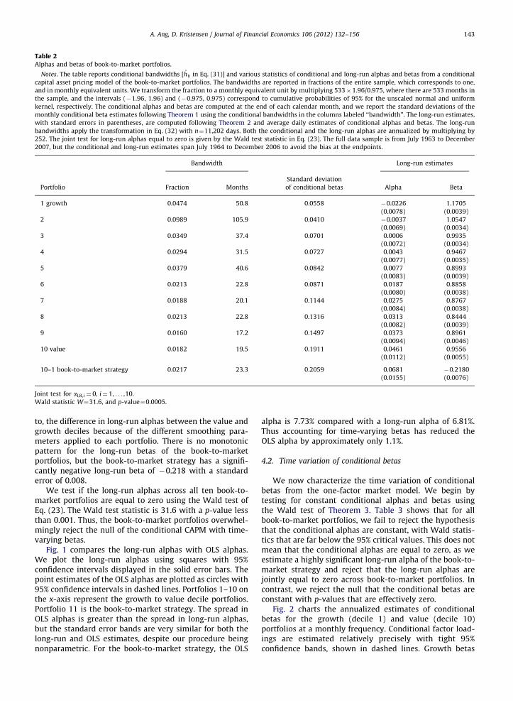
Table 2Alphas and betas of book-to-market portfolios.

Notes. The table reports conditional bandwidths [hk in Eq. (31)] and various statistics of conditional and long-run alphas and betas from a conditional

capital asset pricing model of the book-to-market portfolios. The bandwidths are reported in fractions of the entire sample, which corresponds to one,

and in monthly equivalent units. We transform the fraction to a monthly equivalent unit by multiplying 533�1.96/0.975, where there are 533 months in

the sample, and the intervals (�1.96, 1.96) and (�0.975, 0.975) correspond to cumulative probabilities of 95% for the unscaled normal and uniform

kernel, respectively. The conditional alphas and betas are computed at the end of each calendar month, and we report the standard deviations of the

monthly conditional beta estimates following Theorem 1 using the conditional bandwidths in the columns labeled ‘‘bandwidth’’. The long-run estimates,

with standard errors in parentheses, are computed following Theorem 2 and average daily estimates of conditional alphas and betas. The long-run

bandwidths apply the transformation in Eq. (32) with n¼11,202 days. Both the conditional and the long-run alphas are annualized by multiplying by

252. The joint test for long-run alphas equal to zero is given by the Wald test statistic in Eq. (23). The full data sample is from July 1963 to December

2007, but the conditional and long-run estimates span July 1964 to December 2006 to avoid the bias at the endpoints.

Bandwidth Long-run estimates

Standard deviation

Portfolio Fraction Months of conditional betas Alpha Beta

1 growth 0.0474 50.8 0.0558 �0.0226 1.1705

(0.0078) (0.0039)

2 0.0989 105.9 0.0410 �0.0037 1.0547

(0.0069) (0.0034)

3 0.0349 37.4 0.0701 0.0006 0.9935

(0.0072) (0.0034)

4 0.0294 31.5 0.0727 0.0043 0.9467

(0.0077) (0.0035)

5 0.0379 40.6 0.0842 0.0077 0.8993

(0.0083) (0.0039)

6 0.0213 22.8 0.0871 0.0187 0.8858

(0.0080) (0.0038)

7 0.0188 20.1 0.1144 0.0275 0.8767

(0.0084) (0.0038)

8 0.0213 22.8 0.1316 0.0313 0.8444

(0.0082) (0.0039)

9 0.0160 17.2 0.1497 0.0373 0.8961

(0.0094) (0.0046)

10 value 0.0182 19.5 0.1911 0.0461 0.9556

(0.0112) (0.0055)

10–1 book-to-market strategy 0.0217 23.3 0.2059 0.0681 �0.2180

(0.0155) (0.0076)

Joint test for aLR,i ¼ 0, i¼ 1, . . . ,10.

Wald statistic W¼31.6, and p-value¼0.0005.

A. Ang, D. Kristensen / Journal of Financial Economics 106 (2012) 132–156 143

to, the difference in long-run alphas between the value andgrowth deciles because of the different smoothing para-meters applied to each portfolio. There is no monotonicpattern for the long-run betas of the book-to-marketportfolios, but the book-to-market strategy has a signifi-cantly negative long-run beta of �0.218 with a standarderror of 0.008.

We test if the long-run alphas across all ten book-to-market portfolios are equal to zero using the Wald test ofEq. (23). The Wald test statistic is 31.6 with a p-value lessthan 0.001. Thus, the book-to-market portfolios overwhel-mingly reject the null of the conditional CAPM with time-varying betas.

Fig. 1 compares the long-run alphas with OLS alphas.We plot the long-run alphas using squares with 95%confidence intervals displayed in the solid error bars. Thepoint estimates of the OLS alphas are plotted as circles with95% confidence intervals in dashed lines. Portfolios 1–10 onthe x-axis represent the growth to value decile portfolios.Portfolio 11 is the book-to-market strategy. The spread inOLS alphas is greater than the spread in long-run alphas,but the standard error bands are very similar for both thelong-run and OLS estimates, despite our procedure beingnonparametric. For the book-to-market strategy, the OLS

alpha is 7.73% compared with a long-run alpha of 6.81%.Thus accounting for time-varying betas has reduced theOLS alpha by approximately only 1.1%.

4.2. Time variation of conditional betas

We now characterize the time variation of conditionalbetas from the one-factor market model. We begin bytesting for constant conditional alphas and betas usingthe Wald test of Theorem 3. Table 3 shows that for allbook-to-market portfolios, we fail to reject the hypothesisthat the conditional alphas are constant, with Wald statis-tics that are far below the 95% critical values. This does notmean that the conditional alphas are equal to zero, as weestimate a highly significant long-run alpha of the book-to-market strategy and reject that the long-run alphas arejointly equal to zero across book-to-market portfolios. Incontrast, we reject the null that the conditional betas areconstant with p-values that are effectively zero.

Fig. 2 charts the annualized estimates of conditionalbetas for the growth (decile 1) and value (decile 10)portfolios at a monthly frequency. Conditional factor load-ings are estimated relatively precisely with tight 95%confidence bands, shown in dashed lines. Growth betas

Fig. 1. Long-run alphas versus ordinary-least squares alphas in the

conditional capital asset pricing model for the book-to-market portfo-

lios. Notes. We plot long-run alphas implied by a conditional CAPM and

OLS alphas for the book-to-market portfolios. We plot the long-run

alphas using squares with 95% confidence intervals displayed by the

solid error bars. The point estimates of the OLS alphas are plotted as

circles with 95% confidence intervals in dashed lines. Portfolios 1–10 on

the x-axis represent the growth to value decile portfolios. Portfolio 11 is

the book-to-market strategy, which goes long portfolio 10 and short

portfolio 1. The long-run conditional and OLS alphas are annualized by

multiplying by 252.

Table 3Tests of constant conditional alphas and betas of book-to-market

portfolios.

Notes. We test for constancy of the conditional alphas and betas in a

conditional capital asset pricing model using the Wald test of Theorem 3.

In the columns labeled ‘‘alpha’’ (‘‘beta’’) we test the null that the

conditional alphas (betas) are constant. We report the test statistic W

in Theorem 3 and 95% and 99% critical values of the asymptotic

distribution. We mark rejections at the 99% level with nn.

W Critical values

Portfolio Alpha Beta 95% 99%

1 growth 49 424nn 129 136

2 9 331nn 65 71

3 26 425nn 172 180

4 47 426nn 202 211

5 30 585nn 159 167

6 50 610nn 276 286

7 75 678nn 311 322

8 70 756nn 276 286

9 84 949nn 361 373

10 value 116 1028nn 320 331

10–1 book-to-market strategy 114 830nn 270 280

Fig. 2. Conditional betas of growth and value portfolios. Notes. The

figure shows monthly estimates of conditional conditional betas from a

conditional capital asset pricing model of the first and tenth decile book-

to-market portfolios (growth and value, respectively). We plot 95%

confidence bands in dashed lines. The conditional alphas are annualized

by multiplying by 252.

Fig. 3. Conditional betas of the book-to-market strategy. Notes. The

figure shows monthly estimates of conditional conditional betas of the

book-to-market strategy. We plot the optimal estimates in bold solid

lines along with 95% confidence bands in regular solid lines. We also

overlay the backward 1-year uniform estimates in dashed lines. National

Bureau of Economic Research designated recession periods are shaded in

horizontal bars.

9 The standard error bands of the uniform filters (not shown) are

much larger than the standard error bands of the optimal estimates.

A. Ang, D. Kristensen / Journal of Financial Economics 106 (2012) 132–156144

are largely constant around 1.2, except after 2000, whengrowth betas decline to around one. In contrast, condi-tional betas of value stocks are much more variable,ranging from close to 1.3 in 1965 and around 0.45 in2000. From this low, value stock betas increase to around 1at the end of the sample. We attribute the low relativereturns of value stocks in the late 1990s to the low betas ofvalue stocks at this time.

In Fig. 3, we plot betas of the book-to-market strategy,which is the difference in returns between deciles 10 and 1(value minus growth). Because the conditional betas of

growth stocks are fairly flat, almost all of the time variationof the conditional betas of the book-to-market strategy isdriven by the conditional betas of the decile 10 value stocks.Fig. 3 also overlays estimates of conditional betas from abackward-looking, flat 12-month filter. Similar filters areemployed by Andersen, Bollerselv, Diebold, and Wu (2006)and Lewellen and Nagel (2006). Not surprisingly, the 12-monthuniform filter produces estimates with larger conditionalvariation. Some of this conditional variation is smoothedaway using the longer bandwidths of our optimal estima-tors.9 However, the unconditional variation over the whole

A. Ang, D. Kristensen / Journal of Financial Economics 106 (2012) 132–156 145

sample of the uniform filter estimates and the optimalestimates are similar. For example, the standard deviationof end-of-month conditional beta estimates from the uni-form filter is 0.276, compared with 0.206 for the optimaltwo-sided conditional beta estimates. This implies that theLewellen and Nagel (2006) analysis using backward-lookinguniform filters is conservative. Using our optimal estimatorsreduces the overall volatility of the conditional betas,making it even more unlikely that the value premium canbe explained by time-varying market factor loadings.

Several authors such as Jagannathan and Wang (1996)and Lettau and Ludvigson (2001b) argue that value stockbetas increase during times when risk premia are high,causing value stocks to carry a premium to compensateinvestors for bearing this risk. Theoretical models of riskpredict that betas on value stocks should vary over timeand be highest during times when marginal utility is high(see, for example, Gomes, Kogan, and Zhang, 2003; Zhang,2005). We investigate how betas move over the businesscycle in Table 4 where we regress conditional betas of thevalue-growth strategy onto various macro factors. Kanayaand Kristensen (2010) provide theoretical justification forthis two-step procedure in a continuous-time setting.

In Table 4, we find only weak evidence that the book-to-market strategy betas increase during bad times. Regres-sions I–IX examine the covariation of conditional betas with

Table 4Characterizing conditional betas of the value-growth strategy.

Notes. We regress conditional betas of the value-growth strategy onto variou

pricing model and are plotted in Fig. 3. The dividend yield is the sum of past 1

for Research in Security Prices (CRSP) value-weighted market portfolio. The d

Industrial production is the log year-on-year change in the industrial producti

difference between 10-year Treasury yields and 3-month T-bill yields. Market

market returns over the past month. We denote the Lettau-Ludvigson (2001a)

term trend as cay. Inflation is the log year-on-year change of the CPI index.

variable is a zero-one indicator that takes on the value one if the NBER defin

annualized units. All regressions are at the monthly frequency except regre

premium is constructed in a regression of excess market returns over the nex

rates, industrial production, short rates, term spreads, market volatility, and ca

the market risk premium as the fitted value of this regression at the beginning

denote 95% and 99% significance levels with n and nn, respectively. The data s

Regressor I II III IV

Dividend yield 4.55

(2.01)n

Default spread �9.65

(2.14)nn

Industrial production 0.50

(0.21)

Short rate �1.83

(0.50)nn

Term spread 1.

(1.

Market volatility

cay

Inflation

NBER recession

Market risk premium

Adjusted R2 0.06 0.09 0.01 0.06 0.

individual macro factors known to predict market excessreturns. When dividend yields are high, the market riskpremium is high, and Regression I shows that conditionalbetas covary positively with dividend yields. However, thisis the only variable that has a significant coefficient withthe correct sign. When bad times are proxied by highdefault spreads, high short rates, or high market volatility,conditional betas of the book-to-market strategy tend to belower. During National Bureau of Economic Research desig-nated recessions conditional betas also move the wrongway and tend to be lower. The industrial production, termspread, the Lettau and Ludvigson (2001a) cay, and inflationregressions have insignificant coefficients. The industrialproduction coefficient also has the wrong predicted sign.

In Regression X, we find that book-to-market strategybetas do have significant covariation with many macrofactors. This regression has an impressive adjusted R2 of55%. Except for the positive and significant coefficient onthe dividend yield, the coefficients on the other macrovariables: the default spread, industrial production, shortrate, term spread, market volatility, and cay are eitherinsignificant or have the wrong sign, or both. In RegressionXI, we perform a similar exercise to Petkova and Zhang(2005). We first estimate the market risk premium byrunning a first-stage regression of excess market returnsover the next quarter onto the instruments in Regression X

s macro variables. The betas are computed from a conditional capital asset

2-month dividends divided by current market capitalization of the Centre

efault spread is the difference between BAA and 10-year Treasury yields.

on index. The short rate is the 3-month T-bill yield. The term spread is the

volatility is defined as the standard deviation of daily CRSP value-weighted

cointegrating residuals of consumption, wealth, and labor from their long-

The National Bureau of Economic Research (NBER) designated recession

es a recession that month. All right-hand-side variables are expressed in

ssions VII and XI which are at the quarterly frequency. The market risk

t quarter on dividend yields, default spreads, industrial production, short

y. The instruments are measured at the beginning of the quarter. We define

of each quarter. Robust standard errors are reported in parentheses and we

ample is from July 1964 to December 2006.

V VI VII VIII IX X XI

16.5

(2.95)nn

�1.86

(3.68)

0.18

(0.33)

�7.33

(1.22)nn

08 �3.96

20) (2.10)

�1.38 �0.96

(0.38)nn (0.40)n

0.97 �0.74

(1.12) (1.31)

1.01

(0.55)

�0.07

(0.03)n

0.37

(0.18)n

01 0.15 0.02 0.02 0.01 0.55 0.06

A. Ang, D. Kristensen / Journal of Financial Economics 106 (2012) 132–156146

measured at the beginning of the quarter. We define themarket risk premium as the fitted value of this regressionat the beginning of each quarter. We find that, in Regres-sion XI, there is small positive covariation of conditionalbetas of value stocks with these fitted market risk premiawith a coefficient of 0.37 and a standard error of 0.18. But,the adjusted R2 of this regression is only 0.06. This issmaller than the covariation that Petkova and Zhang(2005) find because they specify betas as linear functionsof the same state variables that drive the time variation ofmarket risk premia. In summary, although conditionalbetas do covary with macro variables, little evidence existsthat betas of value stocks are higher during times when themarket risk premium is high.

4.3. Tests of the conditional Fama and French (1993) model

We now investigate the performance of a conditionalversion of the Fama and French (1993) model estimated onthe book-to-market portfolios and the book-to-market strat-egy. Table 5 reports long-run alphas and factor loadings. Aftercontrolling for the Fama and French factors with time-varyingfactor loadings, the long-run alphas of the book-to-marketportfolios are still significantly different from zero and arepositive for growth stocks and negative for value stocks. Thelong-run alphas monotonically decline from 2.16% for decile1 to �1.58% for decile 10. The book-to-market strategy has along-run alpha of �3.75% with a standard error of 0.010. Thejoint test across all ten book-to-market portfolios for thelong-run alphas equal to zero decisively rejects with a p-value

Table 5Long-run Fama and French (1993) alphas and factor loadings of book-to-mar

Notes. The table reports estimates of long-run alphas and factor loadings fro

market portfolios and the 10–1 book-to-market strategy. The long-run estimat

and average daily estimates of conditional alphas and betas. The long-run alph

equal to zero is given by the Wald test statistic W0 in Eq. (23). The full data sa

July 1964 to December 2006 to avoid the bias at the endpoints.

Portfolio Alpha

1 growth 0.0216

(0.0056)

2 0.0123

(0.0060)

3 0.0072

(0.0067)

4 �0.0057

(0.0072)

5 �0.0032

(0.0075)

6 �0.0025

(0.0072)

7 �0.0113

(0.0071)

8 �0.0153

(0.0057)

9 �0.0153

(0.0069)

10 value �0.0158

(0.0090)

10–1 book-to-market strategy �0.0375

(0.0103)

Joint test for aLR,i ¼ 0, i¼ 1, . . . ,10.

Wald statistic W0¼77.5, and p-value¼0.0000.

of zero. Thus, the conditional Fama and French (1993) modelis overwhelmingly rejected.

Table 5 shows that long-run market factor loadings haveonly a small spread across growth to value deciles, with thebook-to-market strategy having a small long-run marketloading of 0.191. In contrast, the long-run SMB loading isrelatively large at 0.452 and would be zero if the value effectwere uniform across stocks of all sizes. Value stocks have asmall size bias (see Loughran, 1997), and this is reflected in thelarge long-run SMB loading. We expect, and find, that long-runHML loadings increase from �0.672 for growth stocks to 0.792for value stocks, with the book-to-market strategy having along-run HML loading of 1.466. The previously positive long-run alphas for value stocks under the conditional CAPMbecome negative under the conditional Fama and Frenchmodel. The conditional Fama and French model overcompen-sates for the high returns for value stocks by producing SMB

and HML factor loadings that are relatively too large, leading toa negative long-run alpha for value stocks.

In Table 6, we conduct constancy tests of the conditionalalphas and factor loadings. We fail to reject that the condi-tional alphas are constant for all book-to-market portfolios.Whereas the conditional betas exhibited large time variationin the conditional CAPM, we now cannot reject that theconditional market factor loadings are constant for decileportfolios 3–9. However, the extreme growth and valuedeciles do have time-varying MKT betas. Table 6 reportsrejections at the 99% level that the SMB loadings and HML

loadings are constant for the extreme growth and valuedeciles. For the book-to-market strategy, we find strongevidence that the SMB and HML loadings vary over time,

ket portfolios.

m a conditional Fama and French (1993) model applied to decile book-to-

es, with standard errors in parentheses, are computed following Theorem 2

as are annualized by multiplying by 252. The joint test for long-run alphas

mple is from July 1963 to December 2007, but the long-run estimates span

MKT SMB HML

0.9763 �0.1794 �0.6721

(0.0041) (0.0060) (0.0074)

0.9726 �0.0634 �0.2724

(0.0043) (0.0063) (0.0079)

0.9682 �0.0228 �0.1129

(0.0048) (0.0072) (0.0087)

0.9995 0.0163 0.1584

(0.0050) (0.0073) (0.0093)

0.9668 0.0005 0.2567

(0.0053) (0.0079) (0.0099)

0.9821 0.0640 0.3022

(0.0051) (0.0077) (0.0094)

1.0043 0.0846 0.4294

(0.0050) (0.0074) (0.0091)

1.0352 0.1061 0.7053

(0.0041) (0.0061) (0.0075)

1.1011 0.1353 0.7705

(0.0049) (0.0074) (0.0090)

1.1667 0.2729 0.7925

(0.0064) (0.0095) (0.0118)

0.1911 0.4521 1.4660

(0.0073) (0.0108) (0.0133)

Table 6Tests of constant conditional Fama and French (1993) alphas and factor loadings of book-to-market portfolios.

Notes. The table reports W test statistics in Theorem 3 of tests of constancy of conditional alphas and factor loadings from a conditional Fama and

French (1993) model applied to decile book-to-market portfolios and the 10–1 book-to-market strategy. Constancy tests are done separately for each

alpha or factor loading on each portfolio. We report the test statistic W and 95% critical values of the asymptotic distribution. We mark rejections at the

99% level with nn. The full data sample is from July 1963 to December 2007, but the conditional estimates span July 1964 to December 2006 to avoid the

bias at the endpoints.

Portfolio W Critical values

Alpha MKT SMB HML 95% 99%

1 growth 59 441nn 729nn 3259nn 285 295

2 64 369nn 429nn 1035nn 348 360

3 44 184 198 450nn 284 294

4 40 219 209 421nn 236 246

5 31 212 182 675nn 216 225

6 29 201 316nn 773nn 240 436

7 49 195 440nn 1190nn 353 365

8 60 221 483nn 3406nn 369 381

9 37 192 520nn 3126nn 270 281

10 value 42 367nn 612nn 2194nn 242 440

10–1 book-to-market strategy 46 283nn 1075nn 4307nn 257 267

Fig. 4. Conditional Fama and French (1993) loadings of the book-to-

market strategy. Notes. The figure shows monthly estimates of condi-

tional Fama and French (1993) factor loadings of the book-to-market

strategy, which goes long the tenth book-to-market decile portfolio and

short the fist book-to-market decile portfolio. We plot the optimal

estimates in bold lines along with 95% confidence bands in regular lines.

National Bureau of Economic Research designated recession periods are

shaded in horizontal bars.

A. Ang, D. Kristensen / Journal of Financial Economics 106 (2012) 132–156 147

especially for the HML loadings. Consequently, the timevariation of conditional betas in the one-factor model isnow absorbed by time-varying SMB and HML loadings inthe conditional Fama and French model.

We plot the conditional factor loadings in Fig. 4. Marketfactor loadings range between zero and 0.5. The SMB

loadings generally remain above 0.5 until the mid-1970sand then decline to approximately 0.2 in the mid-1980s.During the 1990s the SMB loadings strongly trendedupward, particularly during the late 1990s bull market.This is a period when value stocks performed poorly andthe high SMB loadings translate into larger negative con-ditional Fama and French alphas during this time. After2000, the SMB loadings decrease to end the samplearound 0.25.

Fig. 4 shows that the HML loadings are well above onefor the whole sample and reach a high of 1.91 in 1993 andend the sample at 1.25. Value strategies perform wellcoming out of the early 1990s recession and the early2000s recession, and HML loadings during these periodsdecrease for the book-to-market strategy. One could expectthat the HML loadings should be constant because HML isconstructed by Fama and French (1993) as a zero-costmimicking portfolio to go long value stocks and shortgrowth stocks, which is what the book-to-market strategydoes. However, the breakpoints of the HML factor aredifferent, at approximately thirds, compared to the firstand last deciles of firms in the book-to-market strategy.The fact that the HML loadings vary so much over timeindicates that growth and value stocks in the 10% extremescovary differently with average growth and value stocks inthe middle of the distribution. Put another way, the 10%tail value stocks are not simply levered versions of valuestocks with lower and more typical book-to-market ratios.

5. Portfolios sorted on past returns

We end by testing the conditional Fama and French(1993)model on decile portfolios sorted by past returns.These portfolios are well known to strongly reject the nullof the standard Fama and French model with constantalphas and factor loadings. In Table 7, we report long-runestimates of alphas and Fama and French factor loadingsfor each portfolio and the 10–1 momentum strategy. Thelong-run alphas range from �4.68% with a standard errorof 0.014 for the first loser decile to 2.97% with a standarderror of 0.010 to the tenth loser decile. The momentumstrategy has a long-run alpha of 8.11% with a standarderror of 0.019. A joint test that the long-run alphas areequal to zero rejects with a p-value of zero. Thus, aconditional version of the Fama and French model cannotprice the momentum portfolios.

Table 7 shows that no pattern emerges in the long-runmarket factor loading across the momentum deciles andthe momentum strategy is close to market neutral in the

Table 7Long-run Fama and French (1993) alphas and factor loadings of momentum portfolios.

Notes. The table reports estimates of long-run alphas and factor loadings from a conditional Fama and French (1993) model applied to decile

momentum portfolios and the 10–1 momentum strategy. The long-run estimates, with standard errors in parentheses, are computed following Theorem

2 and average daily estimates of conditional alphas and betas. The long-run alphas are annualized by multiplying by 252. The joint test for long-run

alphas equal to zero is given by the Wald test statistic W0 in Eq. (23). The full data sample is from July 1963 to December 2007, but the long-run estimates

span July 1964 to December 2006 to avoid the bias at the endpoints.

Portfolio Alpha MKT SMB HML

1 losers �0.0468 1.1762 0.3848 �0.0590

(0.0138) (0.0091) (0.0132) (0.0164)

2 0.0074 1.0436 0.0911 0.0280

(0.0103) (0.0072) (0.0102) (0.0128)

3 0.0226 0.9723 �0.0263 0.0491

(0.0087) (0.0061) (0.0088) (0.0111)

4 0.0162 0.9604 �0.0531 0.0723

(0.0083) (0.0058) (0.0084) (0.0104)

5 �0.0056 0.9343 �0.0566 0.0559

(0.0082) (0.0056) (0.0082) (0.0101)

6 �0.0043 0.9586 �0.0363 0.1111

(0.0076) (0.0053) (0.0079) (0.0097)

7 �0.0176 0.9837 �0.0270 0.0979

(0.0074) (0.0052) (0.0077) (0.0094)

8 0.0082 1.0258 �0.0238 0.1027

(0.0073) (0.0052) (0.0077) (0.0095)

9 �0.0078 1.0894 0.0815 0.0337

(0.0078) (0.0055) (0.0081) (0.0101)

10 winners 0.0297 1.2523 0.3592 �0.1753

(0.0103) (0.0074) (0.0183) (0.0135)

10–1 momentum strategy 0.0811 0.0739 �0.0286 �0.1165

(0.0189) (0.0127) (0.0183) (0.0230)

Joint test for aLR,i ¼ 0, i¼ 1, . . . ,10.

Wald statistic W0¼91.0, and p-value¼0.0000.

Fig. 5. Long-run alphas versus ordinary least-squares alphas in the Fama

and French (1993) model for the momentum portfolios. Notes. We plot

long-run alphas from a conditional Fama and French (1993) model and

OLS Fama and French alphas for the momentum portfolios. We plot the

long-run alphas using squares with 95% confidence intervals displayed

in the error bars. The point estimates of the OLS alphas are plotted as

circles with 95% confidence intervals in dashed lines. Portfolios 1–10 on

the x-axis represent the loser to winner decile portfolios. Portfolio 11 is

the momentum strategy, which goes long portfolio 10 and short

portfolio 1. The long-run conditional and OLS alphas are annualized by

multiplying by 252.

A. Ang, D. Kristensen / Journal of Financial Economics 106 (2012) 132–156148

long run with a long-run beta of 0.074. The long-run SMB

loadings are small, except for the loser and winner decilesat 0.385 and 0.359, respectively. These effectively cancel inthe momentum strategy, which is effectively SMB neutral.Finally, the long-run HML loading for the winner portfoliois noticeably negative at �0.175. The momentum strategylong-run HML loading is �0.117, and the negative signmeans that controlling for a conditional HML loadingexacerbates the momentum effect, as firms with negativeHML exposures have low returns on average.

We can judge the impact of allowing for conditionalFama and French loadings in Fig. 5 which graphs the long-run alphas of the momentum portfolios 1–10 and the long-run alpha of the momentum strategy (portfolio 11). Weoverlay the OLS alpha estimates which assume constantfactor loadings. The momentum strategy has a Fama-French OLS alpha of 16.7% with a standard error of 0.026.Table 7 reports that the long-run alpha controlling fortime-varying factor loadings is 8.11%. Thus, the conditionalfactor loadings have lowered the momentum strategyalpha by almost 9% but this still leaves a large amount ofthe momentum effect unexplained. Fig. 5 shows that thereduction of the absolute values of OLS alphas comparedwith the long-run conditional alphas is particularly largefor both the extreme loser and winner deciles.

Fig. 6 shows that all the Fama and French conditionalfactor loadings vary significantly over time and their variationis larger than the case of the book-to-market portfolios.Formal constancy tests (not reported) overwhelmingly rejectthe null of constant Fama and French factor loadings.Whereas the standard deviation of the conditional betas is

around 0.2 for the book-to-market strategy (see Table 2), thestandard deviations of the conditional Fama and French betasare 0.386, 0.584, and 0.658 for MKT, SMB, and HML, respec-tively. Fig. 6 also shows a marked common covariation of

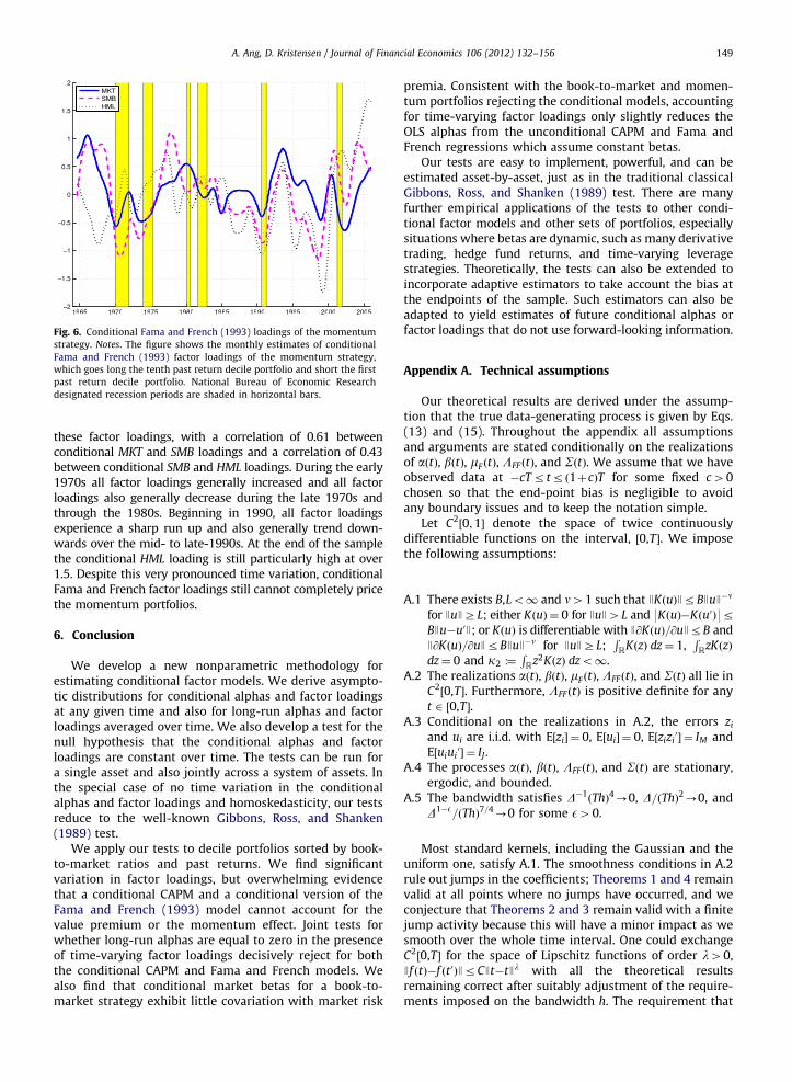
Fig. 6. Conditional Fama and French (1993) loadings of the momentum

strategy. Notes. The figure shows the monthly estimates of conditional

Fama and French (1993) factor loadings of the momentum strategy,

which goes long the tenth past return decile portfolio and short the first

past return decile portfolio. National Bureau of Economic Research

designated recession periods are shaded in horizontal bars.

A. Ang, D. Kristensen / Journal of Financial Economics 106 (2012) 132–156 149

these factor loadings, with a correlation of 0.61 betweenconditional MKT and SMB loadings and a correlation of 0.43between conditional SMB and HML loadings. During the early1970s all factor loadings generally increased and all factorloadings also generally decrease during the late 1970s andthrough the 1980s. Beginning in 1990, all factor loadingsexperience a sharp run up and also generally trend down-wards over the mid- to late-1990s. At the end of the samplethe conditional HML loading is still particularly high at over1.5. Despite this very pronounced time variation, conditionalFama and French factor loadings still cannot completely pricethe momentum portfolios.

6. Conclusion

We develop a new nonparametric methodology forestimating conditional factor models. We derive asympto-tic distributions for conditional alphas and factor loadingsat any given time and also for long-run alphas and factorloadings averaged over time. We also develop a test for thenull hypothesis that the conditional alphas and factorloadings are constant over time. The tests can be run fora single asset and also jointly across a system of assets. Inthe special case of no time variation in the conditionalalphas and factor loadings and homoskedasticity, our testsreduce to the well-known Gibbons, Ross, and Shanken(1989) test.

We apply our tests to decile portfolios sorted by book-to-market ratios and past returns. We find significantvariation in factor loadings, but overwhelming evidencethat a conditional CAPM and a conditional version of theFama and French (1993) model cannot account for thevalue premium or the momentum effect. Joint tests forwhether long-run alphas are equal to zero in the presenceof time-varying factor loadings decisively reject for boththe conditional CAPM and Fama and French models. Wealso find that conditional market betas for a book-to-market strategy exhibit little covariation with market risk

premia. Consistent with the book-to-market and momen-tum portfolios rejecting the conditional models, accountingfor time-varying factor loadings only slightly reduces theOLS alphas from the unconditional CAPM and Fama andFrench regressions which assume constant betas.

Our tests are easy to implement, powerful, and can beestimated asset-by-asset, just as in the traditional classicalGibbons, Ross, and Shanken (1989) test. There are manyfurther empirical applications of the tests to other condi-tional factor models and other sets of portfolios, especiallysituations where betas are dynamic, such as many derivativetrading, hedge fund returns, and time-varying leveragestrategies. Theoretically, the tests can also be extended toincorporate adaptive estimators to take account the bias atthe endpoints of the sample. Such estimators can also beadapted to yield estimates of future conditional alphas orfactor loadings that do not use forward-looking information.

Appendix A. Technical assumptions

Our theoretical results are derived under the assump-tion that the true data-generating process is given by Eqs.(13) and (15). Throughout the appendix all assumptionsand arguments are stated conditionally on the realizationsof aðtÞ, bðtÞ, mF ðtÞ, LFF ðtÞ, and SðtÞ. We assume that we haveobserved data at �cTrtr ð1þcÞT for some fixed c40chosen so that the end-point bias is negligible to avoidany boundary issues and to keep the notation simple.

Let C2½0;1� denote the space of twice continuously

differentiable functions on the interval, ½0,T�. We imposethe following assumptions:

A.1

There exists B,Lo1 and n41 such that JKðuÞJrBJuJ�n

for JuJZL; either KðuÞ ¼ 0 for JuJ4L and 9KðuÞ�Kðu0Þ9rBJu�u0J; or KðuÞ is differentiable with J@KðuÞ=@uJrB andJ@KðuÞ=@uJrBJuJ�n for JuJZL;

RRKðzÞ dz¼ 1,

RRzKðzÞ

dz¼ 0 and k2 :¼RRz2KðzÞ dzo1.

A.2

The realizations aðtÞ, bðtÞ, mF ðtÞ, LFF ðtÞ, and SðtÞ all lie inC2½0,T�. Furthermore, LFF ðtÞ is positive definite for any

t 2 ½0,T�.

A.3 Conditional on the realizations in A.2, the errors zi

and ui are i.i.d. with E½zi� ¼ 0, E½ui� ¼ 0, E½zizi0� ¼ IM and

E½uiui0� ¼ IJ .

A.4

The processes aðtÞ, bðtÞ, LFF ðtÞ, and SðtÞ are stationary,ergodic, and bounded.

A.5

The bandwidth satisfies D�1ðThÞ4-0, D=ðThÞ2-0, and

D1�E=ðThÞ7=4-0 for some E40.

Most standard kernels, including the Gaussian and theuniform one, satisfy A.1. The smoothness conditions in A.2rule out jumps in the coefficients; Theorems 1 and 4 remainvalid at all points where no jumps have occurred, and weconjecture that Theorems 2 and 3 remain valid with a finitejump activity because this will have a minor impact as wesmooth over the whole time interval. One could exchangeC2½0,T� for the space of Lipschitz functions of order l40,

Jf ðtÞ�f ðt0ÞJrCJt�tJl with all the theoretical resultsremaining correct after suitably adjustment of the require-ments imposed on the bandwidth h. The requirement that

A. Ang, D. Kristensen / Journal of Financial Economics 106 (2012) 132–156150

LFFðtÞ40 is a local version of the rank condition knownfrom OLS. The i.i.d. assumption in A.3 can be replaced bymixing or martingale conditions. We however maintain thei.i.d. assumption for simplicity because the proofs otherwisewould become more involved. Since all the moment condi-tions have to hold conditionally on the realizations, A.3rules out leverage effect. We conjecture that leverageeffects can be accommodated by employing argumentssimilar to the ones used in the realized volatility literature,see, e.g., Foster and Nelson (1996). Assumption A.4 isimposed when we analyze the long-run alpha and betaestimators to ensure that the long-run alphas and betas arewell-defined as the limits of sample averages. The condi-tions on the bandwidth in A.5 are needed for the estimatorsof the long-run alphas and betas and when testing the nullof constant alphas or betas. The assumption entails under-smoothing (relative to the point optimal choice of h interms of MSE) in the computation of the long-run estimatesand the test statistics.

Appendix B. Proofs

Proof of Theorem 1. Define h ¼ hT such that bðtÞ can berewritten as

bðtÞ ¼ D2Xn

i ¼ 1

Khðti�tÞf if i

0�Df ðtÞf ðtÞ0

" #�1

� D2Xn

t ¼ 1

Khðti�tÞf iRi

0�Df ðtÞRðtÞ0

" #, ð33Þ

where f ðtÞ ¼DPn

i ¼ 1 Khðti�tÞf i and RðtÞ ¼D

Pni ¼ 1 K

hðti�tÞRi.

Because

f i ¼DFi=D¼ mF ðtiÞþ1ffiffiffiffiDp L1=2

FF ðtiÞui, ð34Þ

we obtain that

f ðtÞ ¼DXn

i ¼ 1

Khðti�tÞmF ðtiÞþ

ffiffiffiffiDp Xn

i ¼ 1

Khðti�tÞL1=2

FF ðtiÞui

¼: f 1ðtÞþ f 2ðtÞ: ð35Þ

Using standard results for Riemann sums and kernel estimators,

f 1ðtÞ ¼DXn

i ¼ 1

Khðti�tÞmF ðtiÞ ¼

Z T

0K

hðs�tÞmF ðsÞ dsþOðDÞ

¼ mF ðtÞþOðh2ÞþOðDÞ: ð36Þ

The second term has mean zero while its variance satisfies

Varðf 2ðtÞÞ ¼DXn

i ¼ 1

K2hðti�tÞLFF ðtiÞ

¼1

hfk2LFF ðtÞþOðh

2ÞþOðDÞg, ð37Þ

where we employ the same arguments as in the analysis of thefirst term. A similar analysis can be carried out for RðtÞ and weconclude that

f ðtÞ ¼ mF ðtÞþOPðh2ÞþOPð1=

ffiffiffih

pÞ,

RðtÞ ¼ aðtÞþbðtÞ0mF ðtÞþOPðh2ÞþOPð1=

ffiffiffih

pÞ: ð38Þ

Similarly,

D2Xn

i ¼ 1

Khðti�tÞf if i

0¼D

Xn

i ¼ 1

Khðti�tÞL1=2

FF ðtiÞuiui0L1=2

FF ðtiÞ

þD2Xn

i ¼ 1

Khðti�tÞmF ðtiÞmF ðtiÞ

0

þD2Xn

i ¼ 1

Khðti�tÞmF ðtiÞui

0L1=2FF ðtiÞ

¼LFF ðtÞþDmF ðtÞmF ðtÞ0þOPðh

2ÞþOPð

ffiffiffiffiffiffiffiffiffiD=h

qÞ, ð39Þ

and

D2Xn

t ¼ 1

Khðti�tÞf iRi

0¼D2

Xn

i ¼ 1

Khðti�tÞf if i

0bðtiÞ

þD2Xn

i ¼ 1

Khðti�tÞf iaðtiÞ

0

þD3=2Xn

i ¼ 1

Khðti�tÞf izi

0S1=2ðtiÞ

¼LFF ðtÞbðtÞþDmF ðtÞaðtÞ0þOPðh

2Þþ

ffiffiffiffiffiffiffiffiffiD=h

qUnðtÞ, ð40Þ

where by a Central Limit Theorem (CLT) for martingales (see,e.g., Brown, 1971),

UnðtÞ :¼ Dffiffiffih

p Xn

i ¼ 1

Khðti�tÞf izi

0S1=2ðtiÞ-

dNð0,k2LFF ðtÞ �SðtÞÞ:

ð41Þ

Collecting the results of Eqs. (37)–(39), we obtain

ffiffiffiffiffiffiffiffiffiffiffiffiD�1h

pD2Xn

i ¼ 1

Khðti�tÞf iRi

0�Df ðtÞRðtÞ0�LFF ðtÞbðtÞ

( )

¼UnðtÞþOPð1Þ-d

Nð0,k2LFF ðtÞ �SðtÞÞ, ð42Þ

and

D2Xn

i ¼ 1

Khðti�tÞf if i

0�Df ðtÞf ðtÞ0 ¼LFF ðtÞþOPð1Þ: ð43Þ

This yields the claimed result. &

Proof of Theorem 2. The proof proceeds along the samelines as in Kristensen (2010, Proof of Theorem 4) and so wesketch only the arguments. First consider bLR. As demon-strated in the proof of Theorem 1, with h ¼ hT ,

bðtÞCXn

i ¼ 1

Khðti�tÞDFiDFi

0

" #�1 Xn

i ¼ 1

Khðti�tÞDFiDFi

0bðtiÞ

" #

þffiffiffiffiDp Xn

i ¼ 1

Khðti�tÞDFiDFi

0

" #�1 Xn

i ¼ 1

Khðti�tÞDFizi

0S1=2ðtiÞ

" #,

ð44Þ

where uniformly over t 2 ½0,T�,

Xn

i ¼ 1

Khðti�tÞDFiDFi

0¼LFF ðtÞþOPðh

2ÞþOPð

ffiffiffiffiffiffiffiffiffiD=h

qÞ: ð45Þ

Thus,

bLR C1

n

Xn

i ¼ 1

Xn

j ¼ 1

L�1FF ðtjÞKh

ðti�tjÞ

8<:

9=;DFiDFi

0bðtiÞ

A. Ang, D. Kristensen / Journal of Financial Economics 106 (2012) 132–156 151

þ

ffiffiffiffiDp

n

Xn

i ¼ 1

Xn

j ¼ 1

L�1FF ðtjÞKh

ðti�tjÞ

8<:

9=;DFizi

0S1=2ðtiÞ

C1

nD

Xn

i ¼ 1

L�1FF ðtiÞDFiDFi

0bðtiÞ

þ1

nffiffiffiffiDp

Xn

i ¼ 1

L�1FF ðtiÞDFizi

0S1=2ðtiÞ

� B1þB2: ð46Þ

Here and in the following, C is used to denote that the leftand right hand side are identical up to some higher-orderterm which is asymptotically negiglible under our assump-tions. Because DFiDFi

0=DCLFF ðtiÞ, B1Cn�1Pn

i ¼ 1 bðtiÞCT�1 R T

0 bðsÞ ds. The second term is a martingale with quad-ratic variation

/B2S¼1

n2D

Xn

i ¼ 1

L�1FF ðtiÞDFiDFi

0L�1FF ðtiÞ �SðtiÞ

C1

n2

Xn

i ¼ 1

L�1FF ðtiÞ � SðtiÞ

C1

nT

Z T

0L�1

FF ðsÞ � SðsÞ ds: ð47Þ

The result for the LR betas now follows by the CLT formartingales together with the Law of Large Numbers (LLN)for stationary and ergodic processes.

Next, consider aLR: With f ðtÞ ¼Pn

i ¼ 1 Khðti�tÞf i and RðtÞ ¼Pn

i ¼ 1 Khðti�tÞRi,

aLR ¼1

n

Xn

j ¼ 1

aðtjÞ ¼1

n

Xn

j ¼ 1

RðtjÞ�bðtjÞf ðtjÞPnj ¼ 1 K

hðti�tjÞ

, ð48Þ

where uniformly over t 2 ½0,T�, DPn

i ¼ 1 Khðti�tÞC1 and

bðtÞCbðtÞ. Thus,

aLR CDn

Xn

j ¼ 1

fRðtjÞ�bðtjÞf ðtjÞg

¼1

nD

Xn

i ¼ 1

DXn

j ¼ 1

Khðti�tjÞ

8<:

9=;Dsi

�1

n

Xn

i ¼ 1

Xn

j ¼ 1

Khðti�tjÞbðtjÞ

8<:

9=;DFi

C1

nD

Xn

i ¼ 1

fDsi�bðtiÞDFig

¼1

n

Xn

i ¼ 1

aðtiÞþ1

nffiffiffiffiDp

Xn

i ¼ 1

S1=2ðtiÞzi � A1þA2: ð49Þ

By the same arguments as for bLR, A1CT�1 R T0 aðsÞ ds, while

A2 is a martingale with quadratic variation

/A2S¼1

n2D

Xn

i ¼ 1

SðtiÞC1

T2

Z T

0SðsÞ ds: ð50Þ

The result for the LR alphas now follows by the CLT formartingales and the LLN for stationary and ergodicprocesses. &

Proof of Theorem 3. The proof follows along the same linesas the proof of Kristensen (2011, Theorem 3.3) and so weonly sketch it. We suppress the index k in the following,and first consider the test statistic for constant alphas,

WðaÞ. Let aðtÞ ¼ a denote the true, constant alpha realiza-tion, and for simplicity suppose that Ft :¼ 0 such that thedata-generating process under HðaÞ is Dsi ¼ aDþ

ffiffiffiffiDp

sðtiÞzi.The extension to Fta0 is straightforward but tedious. Usingthat D

Pnj ¼ 1 K

hðtj�tÞC1 uniformly over t 2 ½0,T�, the non-

parametric estimators of a can therefore be written as

aðtÞ ¼Pn

j ¼ 1 Khðtj�tÞDsj

DPn

j ¼ 1 Khðtj�tÞ

¼ aþPn

j ¼ 1 Khðtj�tÞsðtjÞzjffiffiffiffi

Dp Pn

j ¼ 1 Khðtj�tÞ

CaþffiffiffiffiDp Xn

j ¼ 1

Khðtj�tÞsðtjÞzj, ð51Þ

where h ¼ hT . Because aLR isffiffiffiTp

-consistent, we are allowedto set aLR ¼ a. Also, by the same arguments as in Kristensen(2011, Proof of Theorem 3.3), we can treat sðtÞ as known.Thus,

WðaÞC 1

n

Xn

i ¼ 1

s�2ðtiÞ½aðtÞ�a�2

C1

n

Xn

i ¼ 1

s�2ðtiÞffiffiffiffiDp Xn

j ¼ 1

Khðtj�tÞsðtjÞzj

24

35

2

CDn

Xn

i ¼ 1

Xn

j ¼ 1

Xn

k ¼ 1

s�2ðtiÞKhðtj�tiÞKh

ðtk�tiÞsðtjÞsðtkÞzjzk

¼1

n

Xn

j ¼ 1

DXn

i ¼ 1

K2hðtj�tiÞs�2ðtiÞ

( )s2ðtjÞz

2j

þ1

n

Xjak

DXn

i ¼ 1

Khðtj�tiÞKh

ðtk�tiÞs�2ðtiÞ

( )sðtjÞsðtkÞzjzk,

ð52Þ

where uniformly over tj,tk 2 ½0,T�,

DXn

i ¼ 1

Khðtj�tiÞKh

ðtk�tiÞs�2ðtiÞ

CZ T

0K

hðtj�sÞK

hðtk�sÞs�2ðsÞ ds

C ðKnKÞhðtj�tkÞs�2ðtjÞ: ð53Þ

Thus, with k2 ¼ ðKnKÞð0Þ,

WðaÞC k2

nh

Xn

j ¼ 1

z2j þ

1

n

Xjak

fj,kCk2

hþ

1

n

Xjak

fj,k, ð54Þ

where fj,k :¼ ðKnKÞhðtj�tkÞs�1ðtjÞsðtkÞzjzk. We recognizeP

jakfj,k as a degenerate U-statistic. Because

VarXjak

fj,k

0@

1A¼ 2

Xjak

ðKnKÞ2hðtj�tkÞs�2ðtjÞs2ðtkÞE½z

2j �E½z

2k �

¼ 2Xjak

ðKnKÞ2hðtj�tkÞs�2ðtjÞs2ðtkÞ

C2

D2

Z T

0

Z T

0ðKnKÞ2

hðs�tÞs�2ðsÞs2ðtÞ ds dt

C2

D2h

ZðKnKÞ2ðzÞ dz, ð55Þ

it follows by standard arguments for degenerate U-statis-tics that

ffiffiffih

pDP

jakfj,k-d

Nð0;2RðKnKÞ2ðzÞ dzÞ. In total, with

mðaÞ¼k2=h and v2ðaÞ¼ 2RðKnKÞ2ðzÞ dz=ðT2hÞ, ½WðaÞ�mðaÞ�=

vðaÞ-dNð0;1Þ. This shows the result.

A. Ang, D. Kristensen / Journal of Financial Economics 106 (2012) 132–156152

Next, consider WðbÞ. We focus on the simple casein which aðtÞ ¼ 0 such that, under HðbÞ, Dsi ¼ b0DFiþffiffiffiffiDp

sðtiÞzi. The nonparametric estimators of b can thereforebe written as

bðtÞCbþL�1FF ðtÞ

ffiffiffiffiDp Xn

j ¼ 1

Khðtj�tÞDFjsðtjÞzj, ð56Þ

and we obtain, using that DFjDFj0CDL�1

FF ðtjÞ,

WðbÞC1

n

Xn

i ¼ 1

s�2ðtiÞ½bðtiÞ�b�0LFF ðtiÞ½bðtiÞ�b�

C1

n

Xn

j ¼ 1

s2ðtjÞz2j DFj

0 DXn

i ¼ 1

L�1FF ðtiÞs�2ðtiÞK

2hðtj�tiÞ

( )DFj

þ1

n

Xn

jak

sðtjÞzjDFj0

� DXn

i ¼ 1

L�1FF ðtiÞs�2ðtiÞKh

ðtk�tiÞKhðtj�tiÞ

( )DFksðtkÞzk

Ck2

nh

Xn

j ¼ 1

z2j DFj

0L�1FF ðtjÞDFj

þ1

n

Xn

jak

s�1ðtjÞzjDFj0L�1

FF ðtjÞðKnKÞhðtj�tkÞDFksðtkÞzk

Ck2JD

hþ

1

n

Xn

jak

fj,k, ð57Þ

where fj,k ¼ ðKnKÞhðtj�tkÞDFj0L�1

FF ðtjÞDFks�1ðtjÞsðtkÞzjzk.Pnjak fj,k is a degenerate U-statistic satisfying

VarXjak

fj,k

0@

1A¼ 2D2

Xjak

ðKnKÞ2hðtj�tkÞL

�1FF ðtjÞLFF ðtkÞs�2ðtjÞs2ðtkÞ

C2J

h

ZðKnKÞ2ðzÞ dz, ð58Þ

and soffiffiffih

p Pnjak fj,k-

dNð0;2J

RðKnKÞ2ðzÞ dzÞ. In conclusion,

with mðbÞ ¼ k2JD=h and v2ðbÞ ¼ 2JRðKnKÞ2ðzÞ dz=ðn2hÞ,

½WðbÞ�mðbÞ�=vðbÞ-dNð0;1Þ as desired. &

Appendix C. Conditional alphas

In this section we develop an asymptotic theory for theconditional alpha estimators under the following addi-tional assumption.

A.6

The realizations satisfy aðtÞ ¼ aðt=TÞ, bðtÞ ¼ bðt=TÞ, mF ðtÞ ¼

mF ðt=TÞ, LFF ðtÞ ¼ LFF ðt=TÞ, and SðtÞ ¼ Sðt=TÞ for somefunctions aðtÞ, bðtÞ, mF ðtÞ, LFF ðtÞ, and SðtÞ that all lie inC2½0;1�.

The normalization imposed in A.6 is similar to the oneused in the structural change (or break points) literature.These models are originally developed by, among others,Andrews (1993) and Bai and Perron (1998). Bekaert,Harvey, and Lumsdaine (2002), Paye and Timmermann(2006), and Lettau and Van Nieuwerburgh (2007), amongothers, apply these models in finance. In testing forstructural breaks with one fixed model, the number ofobservations before the break remains fixed as the samplesize increases, n-1, and so the identification of the break

point is not possible. Instead, the literature normalizestime t by sample size n such that the number of observa-tions both before and after the break increases as n-1.This allows the break point and the parameters describingthe coefficients before the break to be identified as n

increases. The same time normalization is also used innonparametric methods for detecting structural change asinitially proposed in Robinson (1989) and further extendedby Cai (2007) and Kristensen (2011). The structural breakspecifications, in which the coefficients take on different(constant) values before and after a break point, are specialcases of our more general model, which allows for a (finite)number of jumps (see Appendix A).

The same idea of employing a sequence of models toconstruct valid asymptotic inference is also used in theliterature on local-to-unity tests introduced by Chan andWei (1987) and Phillips (1987). The local-to-unity modelsemploy a sequence of models indexed by sample size toensure that the same asymptotics apply for both stationaryand nonstationary cases. Analogously, our sequence ofmodels scales the underlying parameters by time span toobtain well-defined asymptotic distributions.

With the time normalization in A.6, the bias of theconditional alpha estimator changes from the one stated inEq. (19) and now becomes E½aðtÞ�CaðtÞþh2að2ÞðtÞ while thevariance in Eq. (19) remains unchanged. Thus, we can nowchoose the bandwidth such that the bias vanishes fasterthan the variance component, and so obtain the followingformal result.

Theorem 4. Assume that assumption A.1–A.3 and A.6 hold

and the bandwidth is chosen such that Th-1 and Th5-0.

Then, for any t 2 ½0,T�,ffiffiffiffiffiffiThpfaðtÞ�aðtÞg �Nð0,k2SðtÞÞ in large samples: ð59Þ

Moreover, the conditional estimators are asymptotically inde-

pendent across any set of distinct time points.

Proof. With t :¼ t=T and ti :¼ ti=T , we can write the esti-mator as aðtÞ ¼ aðtTÞ where

aðtÞ ¼Pn

i ¼ 1 Khðti�tÞfRi�bðtÞ0f igPni ¼ 1 Khðti�tÞ

, ð60Þ

and bðtÞ ¼ bðtTÞ. Given the normalizations in A.6, weobtain by the same arguments used in the proof ofTheorem 1 that bðtÞ ¼ bðtÞþOPðh

2ÞþOPð1=

ffiffiffiffiffiffinhpÞ such that

Ri�bðtiÞ0f iCaðtiÞþS1=2

ðtiÞzi=ffiffiffiffiDp

. This in turn implies that

ffiffiffiffiffiffiThpðaðtÞ�aðtÞÞ ¼OPð

ffiffiffiffiffiffiffiffiTh5

qÞþ

ffiffiffihp

ffiffiffinp

Xn

t ¼ 1

Khðti�tÞS1=2ðtiÞzi,

ð61Þ

where, as Th-1,ffiffiffihp

ffiffiffinp

Xn

t ¼ 1

Khðti�tÞS1=2

ðtiÞzi-d

Nð0,k2SðtÞÞ: & ð62Þ

The crucial assumption in Theorem 4 is the timenormalization in A.6, without which we cannot estimateconditional alphas as discussed in Section 2.5. Given thelarge literature which identifies the constant terms inrolling-window regression estimates as conditional alphas,Theorem 4 can be used to identify these as estimates

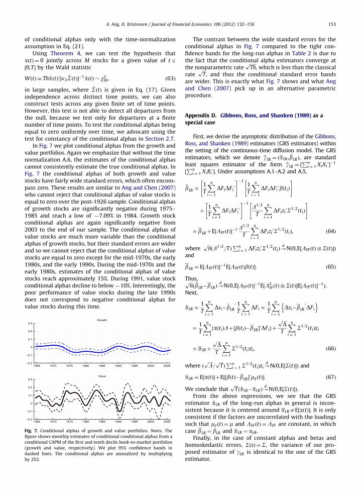
A. Ang, D. Kristensen / Journal of Financial Economics 106 (2012) 132–156 153

of conditional alphas only with the time-normalizationassumption in Eq. (21).

Using Theorem 4, we can test the hypothesis thataðtÞ ¼ 0 jointly across M stocks for a given value of t 2

½0,T� by the Wald statistic

WðtÞ � ThaðtÞ0½k2SðtÞ��1aðtÞ � w2M , ð63Þ

in large samples, where SðtÞ is given in Eq. (17). Givenindependence across distinct time points, we can alsoconstruct tests across any given finite set of time points.However, this test is not able to detect all departures fromthe null, because we test only for departures at a finitenumber of time points. To test the conditional alphas beingequal to zero uniformly over time, we advocate using thetest for constancy of the conditional alphas in Section 2.7.

In Fig. 7 we plot conditional alphas from the growth andvalue portfolios. Again we emphasize that without the timenormalization A.6, the estimates of the conditional alphascannot consistently estimate the true conditional alphas. InFig. 7 the conditional alphas of both growth and valuestocks have fairly wide standard errors, which often encom-pass zero. These results are similar to Ang and Chen (2007)who cannot reject that conditional alphas of value stocks isequal to zero over the post-1926 sample. Conditional alphasof growth stocks are significantly negative during 1975–1985 and reach a low of �7.09% in 1984. Growth stockconditional alphas are again significantly negative from2003 to the end of our sample. The conditional alphas ofvalue stocks are much more variable than the conditionalalphas of growth stocks, but their standard errors are widerand so we cannot reject that the conditional alphas of valuestocks are equal to zero except for the mid-1970s, the early1980s, and the early 1990s. During the mid-1970s and theearly 1980s, estimates of the conditional alphas of valuestocks reach approximately 15%. During 1991, value stockconditional alphas decline to below �10%. Interestingly, thepoor performance of value stocks during the late 1990sdoes not correspond to negative conditional alphas forvalue stocks during this time.

Fig. 7. Conditional alphas of growth and value portfolios. Notes. The

figure shows monthly estimates of conditional conditional alphas from a

conditional CAPM of the first and tenth decile book-to-market portfolios

(growth and value, respectively). We plot 95% confidence bands in

dashed lines. The conditional alphas are annualized by multiplying

by 252.

The contrast between the wide standard errors for theconditional alphas in Fig. 7 compared to the tight con-fidence bands for the long-run alphas in Table 2 is due tothe fact that the conditional alpha estimators converge atthe nonparametric rate

ffiffiffiffiffiffiThp

, which is less than the classicalrate

ffiffiffiTp

, and thus the conditional standard error bandsare wider. This is exactly what Fig. 7 shows and what Angand Chen (2007) pick up in an alternative parametricprocedure.

Appendix D. Gibbons, Ross, and Shanken (1989) as aspecial case

First, we derive the asymptotic distribution of the Gibbons,Ross, and Shanken (1989) estimators (GRS estimators) withinthe setting of the continuous-time diffusion model. The GRSestimators, which we denote ~gLR ¼ ð ~aLR , ~bLRÞ, are standardleast squares estimator of the form ~gLR ¼ ½

Pni ¼ 1 XiXi

0��1

½Pn

i ¼ 1 XiRi0�. Under assumptions A.1–A.2 and A.5,

~bLR C1

T

Xn

i ¼ 1

DFiDFi0

" #�11

T

Xn

i ¼ 1

DFiDFi0bðtiÞ

" #

þ1

T

Xn

i ¼ 1

DFiDFi0

" #�1D1=2

T

Xn

i ¼ 1

DFizi0S1=2ðtiÞ

" #

CbLRþE½LFF ðtÞ��1 D

1=2

T

Xn

i ¼ 1

DFizi0S1=2ðtiÞ, ð64Þ

whereffiffiffinpðD1=2=TÞ

Pni ¼ 1 DFizi

0S1=2ðtiÞ-

dNð0,E½LFF ðtÞ �SðtÞ�Þ

and

bLR ¼ E½LFF ðtÞ��1E½LFF ðtÞbðtÞ�: ð65Þ

Thus,ffiffiffinpð ~bLR�bLRÞ-

dNð0,E½LFF ðtÞ�

�1E½L2FF ðtÞ � SðtÞ�E½LFF ðtÞ�

�1Þ.Next,

~aLR C1

T

Xn

i ¼ 1

Dsi�bLR

0 1

T

Xn

t ¼ 1

DFiC1

T

Xn

i ¼ 1

Dsi�bLR

0DFi

n o

¼1

T

Xn

i ¼ 1

faðtiÞDþ½bðtiÞ�bLR�0DFigþ

ffiffiffiffiDp

T

Xn

i ¼ 1

S1=2ðtiÞzi

CaLRþ

ffiffiffiffiDp

T

Xn

i ¼ 1

S1=2ðtiÞzi, ð66Þ

where ðffiffiffiffiDp

=ffiffiffiTpÞPn

i ¼ 1 S1=2ðtiÞzi-

dNð0,E½SðtÞ�Þ and

aLR ¼ E½aðtÞ�þE½½bðtÞ�bLR�0mF ðtÞ�: ð67Þ

We conclude thatffiffiffiTpð ~aLR�aLRÞ-

dNð0,E½SðtÞ�Þ.

From the above expressions, we see that the GRSestimator ~aLR of the long-run alphas in general is incon-sistent because it is centered around aLRaE½aðtÞ�. It is onlyconsistent if the factors are uncorrelated with the loadingssuch that mF ðtÞ ¼ m and LFF ðtÞ ¼LFF are constant, in whichcase bLR ¼ bLR and aLR ¼ aLR.

Finally, in the case of constant alphas and betas andhomoskedastic errors, SðsÞ ¼S, the variance of our pro-posed estimator of gLR is identical to the one of the GRSestimator.

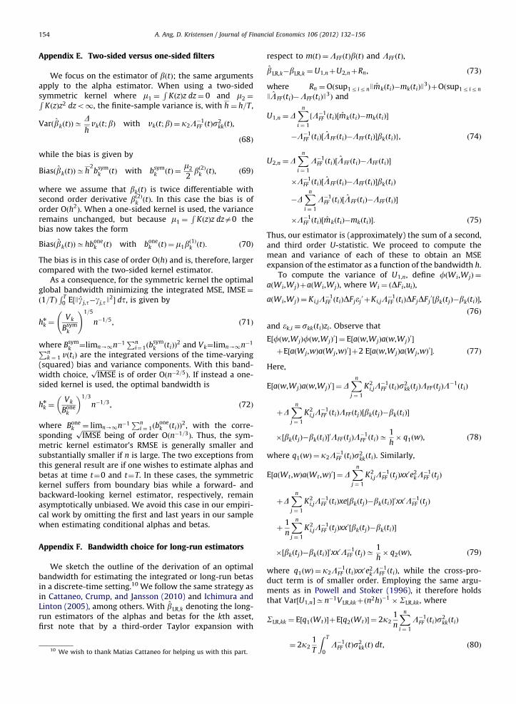
A. Ang, D. Kristensen / Journal of Financial Economics 106 (2012) 132–156154

Appendix E. Two-sided versus one-sided filters

We focus on the estimator of bðtÞ; the same argumentsapply to the alpha estimator. When using a two-sidedsymmetric kernel where m1 ¼

RKðzÞz dz¼ 0 and m2 ¼R

KðzÞz2 dzo1, the finite-sample variance is, with h ¼ h=T ,

VarðbkðtÞÞCDh

vkðt;bÞ with vkðt;bÞ ¼ k2L�1FF ðtÞs

2kkðtÞ,

ð68Þ

while the bias is given by

BiasðbkðtÞÞCh2bsym

k ðtÞ with bsymk ðtÞ ¼

m2

2bð2Þk ðtÞ, ð69Þ

where we assume that bkðtÞ is twice differentiable withsecond order derivative bð2Þk ðtÞ. In this case the bias is oforder Oðh2

Þ. When a one-sided kernel is used, the varianceremains unchanged, but because m1 ¼

RKðzÞz dza0 the

bias now takes the form

BiasðbkðtÞÞChbonek ðtÞ with bone

k ðtÞ ¼ m1bð1Þk ðtÞ: ð70Þ

The bias is in this case of order OðhÞ and is, therefore, largercompared with the two-sided kernel estimator.

As a consequence, for the symmetric kernel the optimalglobal bandwidth minimizing the integrated MSE, IMSE¼ð1=TÞ

R T0 E½Jg j,t�gj,tJ

2� dt, is given by

hn

k ¼Vk

Bsymk

!1=5

n�1=5, ð71Þ

where Bsymk ¼limn-1n�1

Pni¼1ðb

symk ðtiÞÞ

2 and Vk¼limn-1n�1Pnk ¼ 1 vðtiÞ are the integrated versions of the time-varying

(squared) bias and variance components. With this band-width choice,

ffiffiffiffiffiffiffiffiffiffiffiffiIMSEp

is of order Oðn�2=5Þ. If instead a one-sided kernel is used, the optimal bandwidth is

hn

k ¼Vk

Bonek

� �1=3

n�1=3, ð72Þ

where Bonek ¼ limn-1n�1

Pni ¼ 1ðb

onek ðtiÞÞ

2, with the corre-sponding

ffiffiffiffiffiffiffiffiffiffiffiffiIMSEp

being of order Oðn�1=3Þ. Thus, the sym-metric kernel estimator’s RMSE is generally smaller andsubstantially smaller if n is large. The two exceptions fromthis general result are if one wishes to estimate alphas andbetas at time t¼0 and t¼T. In these cases, the symmetrickernel suffers from boundary bias while a forward- andbackward-looking kernel estimator, respectively, remainasymptotically unbiased. We avoid this case in our empiri-cal work by omitting the first and last years in our samplewhen estimating conditional alphas and betas.

Appendix F. Bandwidth choice for long-run estimators

We sketch the outline of the derivation of an optimalbandwidth for estimating the integrated or long-run betasin a discrete-time setting.10 We follow the same strategy asin Cattaneo, Crump, and Jansson (2010) and Ichimura andLinton (2005), among others. With bLR,k denoting the long-run estimators of the alphas and betas for the kth asset,first note that by a third-order Taylor expansion with

10 We wish to thank Matias Cattaneo for helping us with this part.

respect to mðtÞ ¼LFF ðtÞbðtÞ and LFF ðtÞ,

bLR,k�bLR,k ¼U1,nþU2,nþRn, ð73Þ

where Rn ¼Oðsup1r irnJmkðtiÞ�mkðtiÞJ3ÞþOðsup1r irn

JLFF ðtiÞ�LFF ðtiÞJ3Þ and

U1,n ¼DXn

i ¼ 1

fL�1FF ðtiÞ½mkðtiÞ�mkðtiÞ�

�L�1FF ðtiÞ½LFF ðtiÞ�LFF ðtiÞ�bkðtiÞg, ð74Þ

U2,n ¼DXn

i ¼ 1

L�1FF ðtiÞ½LFF ðtiÞ�LFF ðtiÞ�

�L�1FF ðtiÞ½LFF ðtiÞ�LFF ðtiÞ�bkðtiÞ

�DXn

i ¼ 1

L�1FF ðtiÞ½LFF ðtiÞ�LFF ðtiÞ�

�L�1FF ðtiÞ½mkðtiÞ�mkðtiÞ�: ð75Þ

Thus, our estimator is (approximately) the sum of a second,and third order U-statistic. We proceed to compute themean and variance of each of these to obtain an MSEexpansion of the estimator as a function of the bandwidth h.

To compute the variance of U1,n, define fðWi,WjÞ ¼

aðWi,WjÞþaðWi,WjÞ, where Wi ¼ ðDFi,uiÞ,

aðWi,WjÞ ¼ Ki,jL�1FF ðtiÞDFjej

0 þKi,jL�1FF ðtiÞDFjDFj

0½bkðtjÞ�bkðtiÞ�,

ð76Þ

and ek,i � skkðtiÞzi. Observe that

E½fðw,WjÞfðw,WjÞ0� ¼ E½aðw,WjÞaðw,WjÞ

0�

þE½aðWj,wÞaðWj,wÞ0�þ2 E½aðw,WjÞaðWj,wÞ

0�: ð77Þ

Here,

E½aðw,WjÞaðw,WjÞ0� ¼D

Xn

j ¼ 1

K2i,jL�1FF ðtiÞs2

kkðtjÞLFF ðtjÞL�1ðtiÞ

þDXn

j ¼ 1

K2i,jL�1FF ðtiÞLFF ðtjÞ½bkðtjÞ�bkðtiÞ�

�½bkðtjÞ�bkðtiÞ�0LFF ðtjÞL

�1FF ðtiÞC

1

h� q1ðwÞ, ð78Þ

where q1ðwÞ ¼ k2L�1FF ðtiÞs2

kkðtiÞ. Similarly,

E½aðWt ,wÞaðWt ,wÞ0� ¼D

Xn

j ¼ 1

K2i,jL�1FF ðtjÞxx0e2

kL�1FF ðtjÞ

þDXn

j ¼ 1

K2i,jL�1FF ðtiÞxe½bkðtjÞ�bkðtiÞ�

0xx0L�1FF ðtjÞ

þ1

n

Xn

j ¼ 1

K2i,jL�1FF ðtjÞxx0½bkðtjÞ�bkðtiÞ�

�½bkðtjÞ�bkðtiÞ�0xx0L�1

FF ðtjÞC1

h� q2ðwÞ, ð79Þ

where q1ðwÞ ¼ k2L�1FF ðtiÞxx0e2

kL�1FF ðtiÞ, while the cross-pro-

duct term is of smaller order. Employing the same argu-ments as in Powell and Stoker (1996), it therefore holdsthat Var½U1,n�Cn�1VLR,kkþðn

2h�1� SLR,kk, where

SLR,kk ¼ E½q1ðWtÞ�þE½q2ðWtÞ� ¼ 2k21

n

Xn

i ¼ 1

L�1FF ðtiÞs2

kkðtiÞ

¼ 2k21

T

Z T

0L�1

FF ðtÞs2kkðtÞ dt, ð80Þ

A. Ang, D. Kristensen / Journal of Financial Economics 106 (2012) 132–156 155

while VarðU2,nÞ is of higher order and so can be ignored. Intotal,

MSEðgLR,kÞC Bð1ÞLR,k � h2þBð2ÞLR,k �

1

nh

��������

2

þ1

n� VLR,kkþ

1

n2h� SLR,kk: ð81Þ

When minimizing this expression with respect to h, we canignore the two last terms in the above expression sincethey are of higher order (this can be established usinguniform convergence results of, e.g., Kristensen, 2009), andso the optimal bandwidth minimizing the squared compo-nent is

hn

LR ¼½�Bð1Þ0LR,kBð2ÞLR,k=JBð1ÞLR,kJ

2�1=3 � n�1=3, Bð1Þ0LR,kBð2ÞLR,ko0,

½12 Bð1Þ0LR,kBð2ÞLR,k=JBð1ÞLR,kJ2�1=3 � n�1=3, Bð1Þ0LR,kBð2ÞLR,k40,

8<:

ð82Þ

because in general Bð1ÞLR,ka�Bð2ÞLR,k.

References

Aıt-Sahalia, Y., 1996. Nonparametric pricing of interest rate derivativesecurities. Econometrica 64, 527–560.

Aıt-Sahalia, Y., Lo, A., 1998. Nonparametric estimation of state-pricedensities implicit in financial asset prices. Journal of Finance 53,499–547.

Aıt-Sahalia, Y., Brandt, M., 2007. Nonparametric consumption and portfo-lio choice with option-implied state prices. Unpublished workingpaper. Duke University, Durham, NC.

Andersen, T., Bollerselv, T., Diebold, F., Wu, J., 2006. Realized beta:persistence and predictability. In: Fomby, T., Terrell, D. (Eds.),Advances in Econometrics: Econometric Analysis of Economic andFinancial Time Series in Honor of R.F. Engle and C.W.J. Granger, vol. B,Elsevier, Amsterdam, Netherlands, pp. 1–40.

Andrews, D., 1993. Tests for parameter instability and structural changewith unknown change point. Econometrica 61, 821–856.

Ang, A., Chen, J., 2007. CAPM over the long run: 1926–2001. Journal ofEmpirical Finance 14, 1–40.

Ang, A., Chen, J., Xing, Y., 2006. Downside risk. Review of Financial Studies19, 1191–1239.

Ang, A., Kristensen, D., 2011. Testing conditional factor models. Discussionpaper no. 01/2011-030. Tilburg University, Network for Studies onPensions, Aging and Retirement. Tilburg, Netherlands.

Bai, J., Perron, P., 1998. Testing for and estimation of multiple structuralchanges. Econometrica 66, 47–79.

Bandi, F., 2002. Short-term interest rate dynamics: a spatial approach.Journal of Financial Economics 65, 73–110.

Bandi, F., Phillips, P., 2003. Fully nonparametric estimation of scalardiffusion models. Econometrica 71, 241–283.

Barndorff-Nielsen, O., Hansen, P., Lunde, A., Shephard, N., 2009. Multi-variate realized kernels: consistent positive semi-definite estimatorsof the covariation of equity prices with noise and non-synchronoustrading. Journal of Econometrics 162, 149–169.

Bansal, R., Viswanathan, S., 1993. No arbitrage and arbitrage pricing: anew approach. Journal of Finance 48, 1231–1262.

Bekaert, G., Wu, G., 2000. Asymmetric volatility and risk in equitymarkets. Review of Financial Studies 13, 1–42.

Bekaert, G., Harvey, C.R., Lumsdaine, R.L., 2002. The dynamics of emergingmarket equity flows. Journal of International Money and Finance 21(3), 295–350.

Boguth, O., Carlson, M., Fisher, A., Simutin, M., 2011. Conditional risk andperformance evaluation: volatility timing, overconditioning, and newestimates of momentum alphas. Journal of Financial Economics 102,363–389.

Brandt, M., 1999. Estimating portfolio and consumption choice: a condi-tional Euler equations approach. Journal of Finance 54, 1609–1645.

Brown, B.M., 1971. Martingale central limit theorems. Annals of Mathe-matical Statistics 42, 59–66.

Cai, Z., 2007. Trending time-varying coefficient time series models withserially correlated errors. Journal of Econometrics 136, 163–188.

Campbell, J., Cochrane, J., 1999. By force of habit. Journal of PoliticalEconomy 107, 105–251.

Cattaneo, M., Crump, R., Jansson, M., 2010. Generalized jackknife estima-tors of weighted average derivatives. Unpublished working paper.University of Michigan, Ann Arbor, MI.

Chan, N., Wei, C., 1987. Asymptotic inference for nearly nonstationaryAR(1) processes. Annals of Statistics 15, 1050–1063.

Christopherson, J., Ferson, W., Glassman, D., 1998. Conditioning manageralpha on economic information: another look at the persistence ofperformance. Review of Financial Studies 3, 32–43.

Diggle, P., Hutchinson, M., 1989. On spline smoothing with correlatederrors. Australian Journal of Statistics 31, 166–182.

Dimson, E., 1979. Risk measurement when shares are subject to infre-quent trading. Journal of Financial Economics 7, 197–226.

Fama, E., French, K., 1993. Common risk factors in the returns on stocksand bonds. Journal of Financial Economics 33, 3–56.

Fama, E., French, K., 1997. Industry costs of equity. Journal of FinancialEconomics 43, 153–193.

Fama, E., MacBeth, J., 1973. Risk, return, and equilibrium: empirical tests.Journal of Political Economy 81, 607–636.

Fan, J., Zhang, C., Zhang, W., 2001. Generalized likelihood ratio statisticsand Wilks phenomenon. Annals of Statistics 29, 153–193.

Ferson, W., Harvey, C., 1991. The variation of economic risk premiums.Journal of Political Economy 99, 385–415.

Ferson, W., Schadt, R., 1996. Measuring fund strategy and performance inchanging economic conditions. Journal of Finance 51, 425–462.

Ferson, W., Qian, M., 2004. Conditional Evaluation Performance Revisited.Research Foundation of the CFA Institute, Charlotteville, VA.

Foster, D., Nelson, D., 1996. Continuous record asymptotics for rollingsample variance estimators. Econometrica 64, 139–174.

French, K., Schwert, G., Stambaugh, R., 1987. Expected stock returns andvolatility. Journal of Financial Economics 19, 3–29.

Ghysels, E., 1998. On stable factor structures in the pricing of risk: do timevarying betas help or hurt? Journal of Finance 53, 549–574.

Gibbons, M.R., Ferson, W., 1985. Testing asset pricing models withchanging expectations and an unobservable market portfolio. Journalof Financial Economics 14, 217–236.

Gibbons, M.R., Ross, S., Shanken, J., 1989. A test of the efficiency of a givenportfolio. Econometrica 57, 1121–1152.

Gomes, J., Kogan, L., Zhang, L., 2003. Equilibrium cross section of returns.Journal of Political Economy 111, 693–732.

Hardle, W., Hall, P., Marron, J., 1988. How far are automatically chosenregression smoothing parameters from their optimum? Journal of theAmerican Statistical Association 83, 86–101.

Hart, J., 1991. Kernel regression estimation with time series errors. Journalof the Royal Statistical Society, Series B (Methodological) 53, 173–187.

Harvey, C., 2001. The specification of conditional expectations. Journal ofEmpirical Finance 8, 573–638.

Hayashi, T., Yoshida, N., 2005. On covariance estimation of non-synchro-nously observed diffusion Processes. Bernoulli 11, 359–379.

Ichimura, H., Linton, O., 2005. Asymptotic expansions for some semipara-metric program evaluation estimators. In: Andrews, D., Stock, J. (Eds.),Identification and Inference for Econometric Models: A Festschriftfor Tom Rothenberg, Cambridge University Press, Cambridge, UnitedKingdom.

Jagannathan, R., Wang, Z., 1996. The conditional CAPM and the crosssection of expected returns. Journal of Finance 51, 3–53.

Jostova, G., Philipov, A., 2005. Bayesian analysis of stochastic betas. Journalof Financial and Quantitative Analysis 40, 747–778.

Kanaya, S., Kristensen, D., 2010. Estimation of stochastic volatility modelsby nonparametric filtering. Research paper no. 2010-67. Center forResearch in Econometric Analysis of Time Series, University of Aarhus,Denmark.

Kristensen, D., 2009. Uniform convergence rates of kernel estimators withheterogeneous, dependent data. Econometric Theory 25, 1433–1445.

Kristensen, D., 2010. Nonparametric filtering of the realised spot volati-lity: a kernel-based approach. Econometric Theory 26, 60–93.

Kristensen, D., 2011. Nonparametric detection and estimation of struc-tural change. Research paper no. 2011-13. Center for Research inEconometric Analysis of Time Series, University of Aarhus, Denmark.

Lettau, M., Ludvigson, S., 2001a. Consumption, aggregate wealth, andexpected stock seturns. Journal of Finance 56, 815–849.

Lettau, M., Ludvigson, S., 2001b. Resurrecting the (C)CAPM: a cross-sectional test when risk premia are time varying. Journal of PoliticalEconomy 109, 1238–1287.

Lettau, M., Van Nieuwerburgh, S., 2007. Reconciling the return predict-ability evidence. Review of Financial Studies 21, 1607–1652.

Lewellen, J., Nagel, S., 2006. The conditional CAPM does not explain asset-pricing anomalies. Journal of Financial Economics 82, 289–314.

Li, Y., Yang, L., 2011. Testing conditional factor models: a nonparametricapproach. Journal of Empirical Finance 18 (5), 972–992.

A. Ang, D. Kristensen / Journal of Financial Economics 106 (2012) 132–156156

Loughran, T., 1997. Book-to-market across firm size, exchange, andseasonality: is there an effect? Journal of Financial and QuantitativeAnalysis 32, 249–268.

Mamaysky, H., Spiegel, M., Zhang, H., 2008. Estimating the dynamicsof mutual fund alphas and betas. Review of Financial Studies 21,233–264.

Merton, R., 1980. On estimating the expected return on the market.Journal of Financial Economics 8, 323–361.

Mykland, P., Zhang, L., 2006. ANOVA for diffusions and Ito processes.Annals of Statistics 34, 1931–1963.

Newey, W., McFadden, D., 1994. Large sample estimation and hypothesistesting. In: Engle, R., McFadden, D. (Eds.), Handbook of Econometrics,vol. IV, Elsevier, Amsterdam, Netherlands, pp. 2111–2245.

Opsomer, J., Wang, Y., Yang, Y., 2001. Nonparametric regression withcorrelated errors. Statistical Science 16, 134–153.

Paye, B., Timmermann, A., 2006. Instability of return prediction models.Journal of Empirical Finance 13, 274–315.

Petkova, R., Zhang, L., 2005. Is value riskier than growth? Journal ofFinancial Economics 78, 187–202.

Phillips, P., 1987. Towards an unified asymptotic theory for autoregres-sion. Biometrika 74, 535–547.

Powell, J., Stock, J., Stoker, T., 1989. Semiparametric estimation of index

coefficients. Econometrica 57, 1403–1430.Powell, J., Stoker, T., 1996. Optimal bandwidth choice for density-

weighted averages. Journal of Econometrics 75, 291–316.Robinson, P., 1989. Nonparametric estimation of time-varying parameters.

In: Hackl, P. (Ed.), Statistical Analysis and Forecasting of Economic

Structural Changes, Springer-Verlag, Berlin, Germany, pp. 253–264.Ruppert, D., Sheather, S., Wand, M., 1995. An effective bandwidth selector

for local least squares regression. Journal of the American Statistical

Association 90, 1257–1270.Scholes, M., Williams, J., 1977. Estimating betas from non-synchronous

data. Journal of Financial Economics 5, 309–328.Shanken, J., 1990. Intertemporal asset pricing: an empirical investigation.

Journal of Econometrics 45, 99–120.Stanton, R., 1997. A nonparametric model of term structure dynamics

and the market price of interest rate risk. Journal of Finance 52,

1973–2002.Wang, K., 2003. Asset pricing with conditioning information: a new test.

Journal of Finance 58, 161–196.Zhang, L., 2005. The value premium. Journal of Finance 60, 67–103.