statistical testing of covariate effects in conditional
TRANSCRIPT

Electronic Journal of Statistics
Vol. 7 (2013) 2822–2850ISSN: 1935-7524DOI: 10.1214/13-EJS866
Statistical testing of covariate effects in
conditional copula models
Elif F. Acar
Department of StatisticsUniversity of Manitoba
Winnipeg, Manitoba, R3T 2N2, Canadae-mail: [email protected]
Radu V. Craiu
Department of StatisticsUniversity of Toronto
Toronto, Ontario, M5S 3G3, Canadae-mail: [email protected]
and
Fang Yao
Department of StatisticsUniversity of Toronto
Toronto, Ontario, M5S 3G3, Canadae-mail: [email protected]
Abstract: In conditional copula models, the copula parameter is deter-ministically linked to a covariate via the calibration function. The latter isof central interest for inference and is usually estimated nonparametrically.However, in many applications it is scientifically important to test whetherthe calibration function is constant or not. Moreover, a correct model of aconstant relationship results in significant gains of statistical efficiency. Wedevelop methodology for testing a parametric formulation of the calibrationfunction against a general alternative and propose a generalized likelihoodratio-type test that enables conditional copula model diagnostics. We derivethe asymptotic null distribution of the proposed test and study its finitesample performance using simulations. The method is applied to two dataexamples.
AMS 2000 subject classifications: Primary 62H20; secondary 62G10.Keywords and phrases: Constant copula, covariate effects, dynamic cop-ula, local likelihood, model diagnostics, nonparametric inference.
Received August 2012.
1. Introduction
Copulas are an important tool for modeling dependence. The recent develop-ment of conditional copulas by Patton (2006) widely expands the range of possi-ble applications, as it allows covariate adjustment in copula structures and thus
2822

Testing covariate effects in conditional copulas 2823
enables their use in regression settings. Specifically, if X is a covariate that af-fects the dependence between the continuous random variables Y1 and Y2, thenthe conditional joint distribution Hx of Y1 and Y2 given X = x can be written asHx(y1, y2 | x) = Cx{F1|x(y1 | x), F2|x(y2 | x) | x}, where Fi|x is the conditionalmarginal distribution of Yi given X = x for i = 1, 2 and Cx is the conditionalcopula, i.e. the joint distribution of U1 ≡ F1x(Y1 | x) and U2 ≡ F2x(Y2 | x) givenX = x.
When the conditional dependence structure is in the inferential focus, oneneeds to specify a functional connection between the covariateX and the copulaCx as in Jondeau and Rockinger (2006); Patton (2006); Bartram et al. (2007);Rodriguez (2007). Facing the problem of specifying a model for this functionalrelationship, one cannot usually rely on graphical or empirical pointers and musttherefore use flexible models (e.g. semi- or non-parametric) that can potentiallycapture a large variety of patterns. There is now a rich body of work on modellingand estimating conditional copula models, e.g. Gijbels et al. (2011); Abegaz etal. (2012); Veraverbeke et al. (2011); Craiu and Sabeti (2012). In the contextof a parametric copula family, Acar et al. (2011) have studied a nonparametricestimator of the calibration function η(X) in
(U1, U2) | X = x ∼ Cx{u1, u2 | θ(x) = g−1(η(x))}, (1)
where g : Θ → R is a known link function that allows unrestricted estimation forη. In this model, the copula family, i.e. the form of dependence between uniformrandom variables U1 and U2 remains the same for each value of the covariateX = x, but the strength of the dependence between U1 and U2, measured by thecopula parameter θ, is allowed to vary with X according to a smooth functionη. Hence, in order to assess the covariate effect on the strength of dependence,one needs to infer the functional form of η(X).
It is known that if a parametric model for η(X) is suitable, then fitting anonparametric model leads to an unnecessary loss of efficiency. For instance, inTable 1 in Acar et al. (2011) this loss is illustrated in the case of an underlyinglinear calibration function. It is thus of great practical importance to constructrigorous hypothesis tests for the specification of calibration functions.
Our development focuses on the hypotheses of the form H0: “η(·) is linear inX” versus H1: “η(·) is not linear in X” under the conditional copula model in
(1). This class of hypotheses includes the important special case of H(c)0 : “η(·)
is constant” versus H(c)1 : “η(·) is not constant”. In most applications we have
encountered, the constant calibration hypothesis is most relevant scientifically.In comparison, the precise specification of a non-constant calibration function(linear, quadratic, cubic) is of relatively much smaller importance. Therefore,the paper focuses on the constant/nonconstant dichotomy and uses the lin-ear/nonlinear one to illustrate the possible generalizations of the testing proce-dure proposed here. From a statistical viewpoint, it is important to establishthe validity of a constant calibration because then one can rely on inferentialmethods developed for the classical copula model. Canonical approaches basedon likelihood ratio tests are possible when the calibration function is specified
2824 E. F. Acar et al.
parametrically (Jondeau and Rockinger, 2006). Within a Bayesian approach inwhich regression splines are used to model η, Craiu and Sabeti (2012) suggest
that novel criteria for testing H(c)0 are needed.
Hypotheses like H0 cannot be tested using the canonical likelihood ratio test(LRT) because estimation under the alternative hypothesis is performed non-parametrically. Exploration of the asymptotic distribution of the ratio test fallswithin the scope of the generalized likelihood ratio test (GLRT) developed byFan et al. (2001) for testing a parametric null hypothesis versus a nonparametricalternative hypothesis. Since nonparametric maximum likelihood estimators aredifficult to obtain and may not even exist, Fan et al. (2001) suggested using anyreasonable nonparametric estimator under the alternative model. In particular,using a local polynomial estimator to specify the alternative model of a numberof hypothesis testing problems, Fan et al. (2001) showed that the null distri-bution of the GLRT statistic follows asymptotically a chi-square distributionwith the number of degrees of freedom independent of the nuisance parameters.This result, referred to as Wilks phenomenon, holds for Gaussian white-noisemodel (Fan et al., 2001), varying-coefficient models, which include the regres-sion model as a special case (Fan et al., 2001), spectral density (Fan and Zhang,2004), additive models (Fan and Jiang, 2005) and single-index models (Zhanget al., 2010).
We expand the GLRT-based approach to testing the calibration function inconditional copula models. The test procedure employs the nonparametric esti-mator proposed by Acar et al. (2011) when evaluating the local likelihood underthe alternative hypothesis. The major contribution of this work is the construc-tion of a rigorous framework for such GLRTs in the conditional copula context.It is worth mentioning that the proposal can easily accommodate the test for anarbitrary parametric form specified under the null hypothesis. The descriptionof the test, the derivation of its asymptotic null distribution and the discussionof practical implementation are included in Section 2. The finite sample per-formance of the test is illustrated using simulations and two data examples inSection 3 and 4, respectively. The paper ends with concluding remarks.
2. Generalized likelihood ratio test for copula functions
The construction of the GLRT is detailed under the assumption that the condi-tional marginal distributions U1 ≡ F1x(Y1 | x) and U2 ≡ F2x(Y2 | x) are known.A discussion of the impact of estimating the conditional marginal distributionsis provided at the end of this section.
Suppose that {(U11, U21, X1), . . . , (U1n, U2n, Xn)} is a random sample fromthe conditional copula model (1). The null hypothesis of interest restricts thespace of calibration functions to a subspace f that is fully specified paramet-rically. Without loss of generality, we assume f = fL = {η(·) : ∃ a0, a1 ∈R such that η(X) = a0 + a1X, ∀X ∈ X} is the set of all linear functionson X . Then we are interested in testing
H0 : η(·) ∈ fL versus H1 : η(·) /∈ fL. (2)
Testing covariate effects in conditional copulas 2825
In what follows, we assume that the density cx of Cx exists and for simplicitywe use the notation ℓ(t, u1, u2) = ln cx{u1, u2; g
−1(t)}. Furthermore, the firstand second partial derivatives of ℓ with respect to t are assumed to exist andare denoted by ℓj(t, u1, u2) = ∂jℓ(t, u1, u2)/∂t
j , for j = 1, 2.
2.1. Proposed GLRT for the conditional copula model
A natural way to approach (2) is through the likelihood ratio of the restricted(i.e., conditional copula with a linear calibration function) and the full (i.e., con-ditional copula with an arbitrary calibration function) models, or equivalently,through the difference
supη(·)/∈fL
{Ln(H1)} − supη(·)∈fL
{Ln(H0)},
where
Ln(H0) =n∑
i=1
ℓ(a0 + a1Xi, U1i, U2i),
Ln(H1) =
n∑
i=1
ℓ(η(Xi), U1i, U2i).
The supremum of the log-likelihood function under the null hypothesis isgiven by
Ln(H0, η) =n∑
i=1
ℓ(η(Xi), U1i, U2i).
where η(X) = a0 + a1X , with a = (a0, a1) denoting the maximum likelihoodestimator of the parameter a = (a0, a1).
Under the alternative, the general unknown form of η(·) adds significant com-plexity to the calculation of the supremum. We use the nonparametric estimatorof η(·) proposed by Acar et al. (2011) to define the log-likelihood under the fullmodel. Specifically, for each observation Xi in a neighbourhood of an interiorpoint x, we approximate η(Xi) linearly by
η(Xi) ≈ η(x) + η′(x)(Xi − x) ≡ β0 + β1(Xi − x),
provided that η(x) is twice continuously differentiable. Estimates of β = (β0, β1)and of η(x) = β0, are then obtained by maximizing a kernel-weighted locallikelihood function
L(β, x) =n∑
i=1
ℓ{β0 + β1(Xi − x), U1i, U2i}Kh(Xi − x), (3)
where h > 0 is a bandwidth parameter controlling the size of the neighbour-hood around x, K is a symmetric kernel density function and Kh(·) = K(·/h)/h

2826 E. F. Acar et al.
weighs the contribution of each data point based on their proximity to x. Simi-larly, if one uses a pth order local polynomial estimator, the local linear approxi-mation in (3) will be replaced by
∑pℓ=0 βℓ(Xi−x)ℓ and the resulting estimator is
given by ηh(x) = β0. The bandwidth h is chosen to maximize the cross-validationcriterion
B(h) =n∑
i=1
ln c(U1i, U2i | θ(−i)h (Xi)),
where θ(−i)h (Xi) is the estimate of the copula parameter θ at Xi when the ith
sample (U1i, U2i) is left out.Then we evaluate the log-likelihood function under the alternative hypothesis
of (2) as
Ln(H1, ηh) =
n∑
i=1
ℓ{ηh(Xi), U1i, U2i}.
The difference between the two log-likelihoods allows us to evaluate the evi-dence in the data in favor of (or against) the null model. Hence, the generalizedlikelihood ratio statistic is given by
λn(h) = Ln(H1, ηh)− Ln(H0, η). (4)
While large values of λn(h) suggest the rejection of the null hypothesis, we needto determine the rejection region for the test. In order to inform the decision infinite samples we investigate the asymptotic distribution of the GLRT statisticunder the null hypothesis.
2.2. Asymptotic distributions of proposed GLRT statistic
To facilitate our presentation we introduce the following notation. Let f(x) > 0be the density function of X with support X and denote by |X | the range of thecovariate X . Also, denote by K ∗K the convolution of the kernel K and define
µn =|X |h
(K(0)− 1
2
∫K2(t)dt
)=
|X |h
cK ,
νn =2|X |h
∫(K(t)− 1
2K ∗K(t))2dt,
cK = K(0)− 1
2
∫K2(t)dt.
The following result states that the GLRT statistic follows asymptotically anormal or equivalently a chi-square distribution in the case of negligible bias,where the mean and variance are related to the quantities µn and νn, respec-tively. The technical conditions and proofs are deferred to Appendix I.
Theorem 1. Assume that the conditions (A1)–(A7) in Appendix I hold andthe GLRT statistic λn(h) is constructed from (4) with a local linear estimator.

Testing covariate effects in conditional copulas 2827
Then, as h → 0 and nh3/2 → ∞,
ν−1/2n (λn(h)− µn + dn)
L−→ N(0, 1), (5)
where dn = Op(nh4 + n1/2 h2).
Furthermore, if η is linear or nh9/2 → 0, then, as nh3/2 → ∞,
rKλn(h)asym∼ χ2
rK µn, (6)
where rK = 2 µn/νn.
2.3. Practical implications and further aspects
In order to use the asymptotic result proven in Theorem 1 in a practical setting,one needs to choose values for the bandwidth parameter and the order of thepolynomial fitting. We give below guidelines for these choices and discuss otheraspects relevant to the implementation of the GLRT.
Choice of bandwidth parameter. It should be noted that when η is linear, theasymptotic bias dn becomes exactly zero, as shown in (8) in the Appendix I,and thus the condition nh9/2 → 0 is not needed (the optimal bandwidth forestimation is of the order n−1/5, see Acar et al., 2011). More importantly, thisfacilitates the calculation of the GLRT statistic λn(h) in practice, since onecan use directly the bandwidth used for estimation, chosen by the leave-one-outcross-validated likelihood (Acar et al., 2011). Our simulation study in Section 3provides empirical support for this suggestion.
Order of local polynomial fitting and testing polynomial functions. The asymp-totic results in Theorem 1 can be easily extended to the case where λn(h) isbased on a pth order local polynomial estimator, by substituting the kernelfunction K with its equivalent kernel K∗ in cK and rK (see Fan and Gijbels,1996, page 64, for the expression of K∗) induced by the local polynomial fit-ting (Fan et al., 2001). The asymptotic chi-square distribution (6) continues tohold if either η is a polynomial of degree p or nh(4p+5)/2 → 0, as the asymp-totic bias dn = Op(nh
2p+2 + n1/2hp+1). The practical implication of such anextension is that, if the interest is to test a null hypothesis of a polynomialform η(x) =
∑pℓ=0 βℓx
ℓ, it is recommended to calculate λn(h) using the localpolynomial estimator with the corresponding degree p. This avoids the possiblenecessity of undersmoothing in order to have the asymptotic bias negligible.
Testing constancy of the copula parameter. As pointed out earlier, the hypoth-esis of η being constant is a special case of the linearity constraint and leadsto the classical copula model (i.e., no covariate adjustment is required). If thishypothesis is of interest, using a local constant estimator, i.e., p = 0, to calculateλn(h) may be more appealing (as confirmed by the simulations in Section 3)than using a local linear estimator. The latter tends to overfit even with largebandwidth when H0 indeed holds, thus resulting in an inflated type I error.

2828 E. F. Acar et al.
Testing independence. While the test is quite general and can be used, in prin-ciple, to test any preset copula parameter value, extra caution is needed whentesting independence. Under the null hypothesis of independence, the copula pa-rameter is at the boundary of the parameter space (e.g., θ = 0 for the Frank andClayton families, and θ = 1 for the Gumbel family), and the asymptotic result inTheorem 1 does not hold. For the canonical likelihood ratio test, the asymptoticnull distribution is known to be a mixture of chi-squares when some parameterslie on boundary of the parameter space (Self and Liang, 1987). A similar resultis expected to hold for the GLRT as the two tests are fairly similar in nature (seethe next paragraph). However, an investigation in this direction may not be toomuch of practical value, considering that there are a number of independencetests in the copula literature (see, for instance, Genest and Remillard, 2004).
Relationship to the canonical likelihood ratio test. One can conclude from The-orem 1 that the GLRT is fairly similar to the classical likelihood ratio test.The tabulated value of the scaling constant rK is close to 2 for commonly usedkernels. For instance, rK = 2.115 for the commonly used Epanechnikov kernelK(u) = 0.75(1 − u2)1{|u|≤1}. The degrees of freedom (df) rK cK |X |/h of theasymptotic null distribution of the GLRT tends to infinity when h → 0, dueto the nonparametric nature of the alternative hypothesis. One can interpretthe quantity |X |/h as the number of nonintersecting intervals on X , and thusrK cK |X |/h approximates the effective number of parameters in the nonpara-metric estimation. For the Epanechnikov kernel with cK = 0.45, the degrees offreedom is given by 0.968 |X |/h.Impact of estimating conditional marginal distributions. An important aspect in(conditional) copula model implementation is the estimation of unknown (con-ditional) marginal distributions. Although the proposed GLRT procedure waspresented assuming that the conditional marginal distributions are known, The-orem 1 provides a basis for more general approach where estimation is performedjointly or using a two-step method (i.e., parameters for the marginal distribu-tions are estimated first and only subsequently the inference for the conditionalcopula parameters is performed).
In a conditional copula model with parametric conditional marginal distri-butions, one can easily accommodate joint estimation under the null hypoth-esis since the model for the calibration function is then parametric. On theother hand, joint analysis under the alternative requires iterative estimationof parametric conditional marginal distributions and nonparametric calibrationfunction model. Although, such iterative procedures have been long studied fornonparametric regression problems, for instance in partially linear models, theproblem of joint estimation has not been addressed yet in the conditional copulasetting.
As shown in Appendix I, the asymptotic distribution of the GLR statis-tic λn(h) is governed by the nonparametric part λ1n(h) since the parametricpart λ2n, which corresponds to the canonical likelihood ratio statistic, vanishescompared to λ1n(h). Hence, even one employs joint maximum likelihood esti-mation or a less efficient inference for margins approach (Joe, 2005) under the

Testing covariate effects in conditional copulas 2829
null hypothesis, the result in Theorem 1 will not change. Generally speaking,the proposed test remains valid as long as the conditional marginal distributionsare estimated with the usual parametric rate
√n, both under the null and under
the alternative (see Remark 1 at the end of Appendix I). A two-step approachcan be safely employed in the testing procedure provided that the conditionalmarginal distributions are estimated parametrically. This observation, in fact,motivated the use of parametric models to specify the conditional marginal dis-tributions in the data examples of Section 4. Note that an alternative two-stepapproach is to use kernel-based smoothing methods as in Abegaz et al. (2012) inthe first stage. However, this case requires a careful treatment as both the nulland the alternative models will have nonpararametric convergence rates due tononparametric specification of the conditional marginal distributions.
Choice of copula family. The proposed GLRT approach assumes that the truecopula family is used in the test procedure. If the copula is misspecified, theasymptotic result in Theorem 1 would not hold. This phenomenon is similar tothe departures from the chi-squared asymptotic limit exhibited by the canonicallikelihood ratio tests under misspecified models. Furthermore, copula misspec-ification can lead to serious bias in the estimation results. Nonetheless, in oursimulations we have observed a good performance of the cross-validated predic-tion error criterion of Acar et al. (2011) in choosing the true copula family.
3. Simulation study
We conduct simulations to evaluate the finite sample performance of the pro-posed test for the linear hypothesis given in (2). We consider four simulationscenarios corresponding to four calibration functions,
M(F )0 : η0(X) = 8,
M(F )1 : η1(X) = 25− 4.2X,
M(F )2 : η2(X) = 1 + 2.5(3−X)2,
M(F )3 : η3(X) = 12 + 8 sin(0.4X2).
The copula used belongs to the Frank family and has the form
C(u1, u2|θ) = −1
θln
{1 +
(e−θu1 − 1)(e−θu2 − 1)
e−θ − 1
}, θ ∈ (−∞,∞) \ {0}.
Since the range of θ is R \{0} for the Frank copula, an identity link is used, i.e.,θk(X) = ηk(X) for k = 0, 1, 2, 3. Similar findings, summarized in Appendix II,were obtained in simulations produced using the Clayton and Gumbel copulasin the true generating models.
As mentioned earlier, the copula family describes the overall shape of thedependence. For the Frank family, this shape is symmetric and shows no taildependence as shown in the left panel of Figure 1. The four calibration models
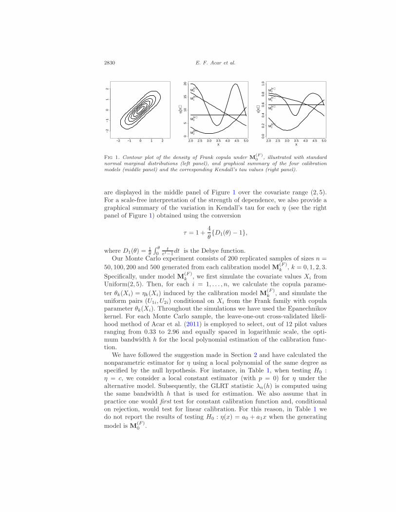
2830 E. F. Acar et al.
−2 −1 0 1 2
−2
−1
01
2
2.0 2.5 3.0 3.5 4.0 4.5 5.0
05
1015
20
X
η(X
)
M2(F)
M0(F)
M1(F)
M3(F)
2.0 2.5 3.0 3.5 4.0 4.5 5.0
0.0
0.2
0.4
0.6
0.8
1.0
X
τ(X
)
M2(F)
M0(F)
M1(F)
M3(F)
Fig 1. Contour plot of the density of Frank copula under M(F )0 , illustrated with standard
normal marginal distributions (left panel), and graphical summary of the four calibrationmodels (middle panel) and the corresponding Kendall’s tau values (right panel).
are displayed in the middle panel of Figure 1 over the covariate range (2, 5).For a scale-free interpretation of the strength of dependence, we also provide agraphical summary of the variation in Kendall’s tau for each η (see the rightpanel of Figure 1) obtained using the conversion
τ = 1 +4
θ{D1(θ) − 1},
where D1(θ) =1θ
∫ θ
0t
et−1dt is the Debye function.Our Monte Carlo experiment consists of 200 replicated samples of sizes n =
50, 100, 200 and 500 generated from each calibration model M(F )k , k = 0, 1, 2, 3.
Specifically, under model M(F )k , we first simulate the covariate values Xi from
Uniform(2, 5). Then, for each i = 1, . . . , n, we calculate the copula parame-
ter θk(Xi) = ηk(Xi) induced by the calibration model M(F )k , and simulate the
uniform pairs (U1i, U2i) conditional on Xi from the Frank family with copulaparameter θk(Xi). Throughout the simulations we have used the Epanechnikovkernel. For each Monte Carlo sample, the leave-one-out cross-validated likeli-hood method of Acar et al. (2011) is employed to select, out of 12 pilot valuesranging from 0.33 to 2.96 and equally spaced in logarithmic scale, the opti-mum bandwidth h for the local polynomial estimation of the calibration func-tion.
We have followed the suggestion made in Section 2 and have calculated thenonparametric estimator for η using a local polynomial of the same degree asspecified by the null hypothesis. For instance, in Table 1, when testing H0 :η = c, we consider a local constant estimator (with p = 0) for η under thealternative model. Subsequently, the GLRT statistic λn(h) is computed usingthe same bandwidth h that is used for estimation. We also assume that inpractice one would first test for constant calibration function and, conditionalon rejection, would test for linear calibration. For this reason, in Table 1 wedo not report the results of testing H0 : η(x) = a0 + a1x when the generating
model is M(F )0 .

Testing covariate effects in conditional copulas 2831
Table 1
Demonstration of the proposed GLRT for testing the linear/constant null hypothesis H0 atα = 0.10, 0.05 and 0.01, respectively, under the Frank copula. Shown are the rejection
frequencies assessed from 200 Monte Carlo replicates. The sample sizes are n = 50, 100, 200and 500; the generating calibration models are shown in the “True Model” column. Thoseentries in the table reflecting the power of the testing procedure are shown in bold face
Null ModelTrue Model H0 : η(x) = a0 + a1x H0 : η = c
n .10 .05 .01 .10 .05 .0150 — — — .075 .025 .015100 — — — .110 .055 .010200 — — — .105 .040 .020M
(F )0
500 — — — .110 .045 .00550 .060 .020 .005 .695 .520 .255
100 .100 .060 .010 .910 .870 .760
200 .100 .055 .005 .995 .990 .955M(F )1
500 .085 .055 .010 1.00 1.00 1.00
50 .425 .285 .085 .640 .515 .255
100 .650 .510 .245 .940 .860 .620
200 .895 .790 .560 1.00 1.00 .975M(F )2
500 1.00 1.00 .980 1.00 1.00 1.00
50 .735 .635 .435 .755 .645 .385
100 .865 .840 .780 .965 .945 .870
200 1.00 1.00 1.00 1.00 1.00 1.00M(F )3
500 1.00 1.00 1.00 1.00 1.00 1.00
One can notice from Table 1 that the rejection rates under the null are veryclose to the target values of the type I error probabilities α ∈ {0.1, 0.05, 0.01},for both linear and constant nulls (models M
(F )0 and M
(F )1 ), except for the case
with n = 50, which is slightly conservative. Since nonparametric methods oftenrequire relatively large samples, the latter observation confirms that caution isrecommended when working with small samples. Overall, our approach leads tohigh power in detecting departures from the null, as one can see from the results
generated under models M(F )1 , M
(F )2 and M
(F )3 . For clearer visualization, the
entries in the table that correspond to power are shown in bold face. As expected,the rejection rates increase with the sample size and the nonlinearity of theunderlying calibration function (see the middle or right panel of Figure 1 for avisual comparison). For instance, when testing the linear calibration hypothesis,
we observe lower rejection rates for M(F )2 , which is quadratic, than for M
(F )3 ,
which exhibits more variation.
4. Data application
In this section, we apply the GLRT to the two data examples studied in Acaret al. (2011). Our aim is to check whether a constant copula model or a condi-tional copula model with a linear calibration function fits these examples rea-sonably well, i.e. whether the nonparametric calibration estimates of Acar et al.(2011) are in fact necessary.

2832 E. F. Acar et al.
0.0 0.2 0.4 0.6 0.8 1.0
0.0
0.2
0.4
0.6
0.8
1.0
U1
U2
30 35 40
24
68
1012
14
GA
η(G
A)
30 35 40
0.0
0.2
0.4
0.6
0.8
1.0
GA
τ(G
A)
Fig 2. Scatterplot of transformed birth weights (left panel), and the plots of calibration func-tion estimates (middle panel) and the corresponding Kendall’s tau values (right panel) underthe Frank copula: maximum likelihood estimate of the constant calibration function (solidline), maximum likelihood estimate of the linear calibration function (long-dashed line), lo-cal constant estimates (dot-dashed line), local linear estimates (dashed line), 90% pointwiseconfidence intervals for the local linear estimates (dotted lines).
4.1. Twin birth data
This data set contains information on 450 pairs of twins from the MatchedMultiple Birth Data Set (MMB) of the National Center for Health Statistics.We consider the birth weights (BW1, BW2) of the first- and second-born twinswho survived their first year, and whose mothers were between 18 and 40 yearsold. The gestational age GA is an important factor for fetal growth and istherefore included in the analysis as a covariate. The question of interest hereis whether the dependence between the weights BW1 and BW2 varies with GA.Subsequent interrogations regarding the exact parametric forms of η are muchless relevant. We transform the data on the uniform scale, as shown in the leftpanel of Figure 2, after fitting parametric marginal regression models. We usethe Frank family of copulas to model the dependence structure, as this was thefamily chosen by Acar et al. (2011) according to their cross-validated predictionerror criterion. The middle panel of Figure 2 shows the maximum likelihoodestimates obtained under the constant calibration assumption (solid line), linearcalibration assumption (long-dash line), the nonparametric estimates with p = 0(dot-dashed line), p = 1 (dashed line) and 90% pointwise confidence intervalsfor the local linear estimates (dotted lines), obtained as in Acar et al. (2011).These results are also displayed in terms of Kendall’s tau in the right panel ofFigure 2.
As seen in Figure 2, the maximum likelihood estimates under constant andlinear calibration assumptions are not within the pointwise confidence inter-vals of the local linear estimates, suggesting that these simple parametric for-mulations may not be appropriate. This empirical observation is confirmed bythe GLRT tests, which yielded p-values smaller than 10−5 for both tests (teststatistics are 13.58 on 3.92 df and 12.95 on 3.36 df for the constant and linearhypothesis, respectively).
Thus, we conclude that the variation in the strength of dependence betweenthe twin birth weights at different gestational ages, as represented by the non-

Testing covariate effects in conditional copulas 2833
0.0 0.2 0.4 0.6 0.8 1.0
0.0
0.2
0.4
0.6
0.8
1.0
U1
U2
−4 −2 0 2 4
02
46
∆BMIη(
∆BM
I)−4 −2 0 2 4
0.0
0.2
0.4
0.6
0.8
1.0
∆BMI
τ(∆B
MI)
Fig 3. Scatterplot of the transformed log-pulse pressures (left panel), and the plots of cali-bration function estimates (middle panel) and the corresponding Kendall’s tau values (rightpanel) under the Frank copula: maximum likelihood estimate of the constant calibration func-tion (solid line), maximum likelihood estimate of the linear calibration function (long-dashedline), local constant estimates (dot-dashed line), local linear estimates (dashed line), 90%pointwise confidence intervals for the local linear estimates (dotted lines).
parametric estimates in the right panel of Figure 2 is statistically significant.The estimated nonlinear pattern indicates a relatively stronger dependence be-tween the birth weights of the preterm (28-32 weeks) and post-term (38-42weeks) twins compared to the twins delivered at term (33-37 weeks). While thefactors affecting the twin fetal growth patterns are not fully known, the rela-tively stronger intra-twin dependence for preterm twins may be due to the factthat fat accumulation only begins in the third trimester of gestation (around 28weeks). Hence, during the weeks 28-32, twins are expected to be still very simi-lar in their growth. The increase in the strength of dependence after week 38, onthe other hand, is more puzzling, but perhaps can be explained by intrauterinegrowth restriction factors.
4.2. Framingham heart study data
This data set comes from the Framingham Heart Study (FHS) and containsthe log-pulse pressures of 348 subjects at the first two examination periods(1956 and 1962), denoted by log(PP1) and log(PP2), respectively, as well asthe change in body mass index ∆BMI between these periods. Pulse pressure,defined as the difference between systolic and diastolic blood pressure, reflectsarterial stiffness and is associated with an increased risk in stroke incidence.For the 348 subjects, who experienced a stroke during the rest of follow-upperiod, of interest is to investigate the dependence structure between log(PP1)and log(PP2) conditional on ∆BMI. The left panel of Figure 3 displays theconditional marginal distributions of the log-pulse pressures given ∆BMI, whichare obtained parametrically as in Acar et al. (2011).
In conditional copula selection, Acar et al. (2011) used the cross-validatedprediction errors only for the second log-pulse pressure as the selection criterion,and chose the Frank copula family. Proceeding with their choice, we obtained the

2834 E. F. Acar et al.
calibration function estimates using the maximum likelihood estimation withconstant and linear calibration forms and the nonparametric estimation withp = 0 and p = 1. The results are shown in the middle panel of Figure 3, andconverted to the Kendall’s tau scale in the right panel.
Based on the Figure 3 we suspect that a constant copula model may be appro-priate, even though it is not fully contained in the pointwise confidence intervals.Note that the latter provides only partial guidance, and simultaneous confidenceintervals are needed for a decisive visual conclusion. To decide whether the fit-ted constant copula model is appropriate, we perform the GLRT using the localconstant estimates at the bandwidth value h = 3.45. This bandwidth choiceleads to 2.66 df of the chi-square distribution. The difference between the log-likelihoods of the alternative and null conditional copula models is 0.91 andconsequently the p-value is 0.514. Thus, we conclude that the change in bodymass index does not have any significant effect on the strength of dependencebetween the two log-pulse pressures.
5. Conclusion
Adjusting statistical dependence for covariates via conditional copulas is an ac-tive area of research where model fitting and validation are currently in early de-velopment. This paper takes a first step towards establishing conditional copulamodel diagnostics by presenting a formal test of hypothesis for the calibrationfunction. Inspired by the generalized likelihood ratio idea of Fan et al. (2001),the proposed test uses the local likelihood estimator of Acar et al. (2011) tospecify the model under the alternative when testing a parametric calibrationfunction hypothesis. The asymptotic null distribution of the test statistic, shownto be a chi-squared distribution with the number of degrees of freedom deter-mined by the estimation-optimal bandwidth, is used to determine the rejectionregion in finite samples. Simulations suggest that the method has high power ofdetecting departures from the null model and yields the targeted type I errorprobability.
The GLRT procedure presented here can be easily adapted to test an ar-bitrary parametric calibration function. Furthermore, the approach can be ex-tended to employ other nonparametric estimators, such as smoothing splines,although with additional effort of deriving the asymptotic null distribution. Nev-ertheless, the asymptotic null distribution may not always be appropriate fordetermining the rejection region in finite samples. While conditional bootstrapis usually used to assess the null distribution of the GLRT in regression-basedproblems, defining a similar bootstrap procedure in the conditional copula set-ting is not straightforward and requires further study.
Although the focus of the paper is on bivariate copulas, the GLRT approachis potentially applicable to multivariate copulas. However, complications arisein the latter case since the number of copula parameters is likely to increaseand simultaneous testing is therefore necessary. This represents an interestingdirection for future research.

Testing covariate effects in conditional copulas 2835
One current restriction of the test is that it requires the covariate to be uni-variate. This restriction is mainly due to the lack of a nonparametric estimationprocedure that can accommodate multiple covariates. The latter is subject ofongoing research together with a covariate selection method based on the GLRTframework.
Appendix I: Regularity conditions and technical proofs
The asymptotic distribution of the GLRT statistic relies on the following tech-nical conditions. The conditions (A1)–(A3) are standard in nonparametric esti-mation and the conditions (A4)–(A7) are required to regularize the conditionalcopula density.
(A1) The density function f(X) > 0 of the covariate X is Lipschitz continuous,and X has a bounded support X .
(A2) The kernel function K(t) is a symmetric probability density function thatis bounded and Lipschitz continuous.
(A3) The functions η and g−1 have (p+1)th continuous derivatives, where p = 1when a local linear estimator is used for λn(h).
(A4) The functions ℓ1{η(x), u1, u2} and ℓ2{η(x), u1, u2} exist and are continuouson X × (0, 1)2, and can be bounded by integrable functions of u1 and u2.
(A5) E∣∣{ℓ1(η(x), u1, u2) | x}
∣∣4 < ∞.(A6) E{ℓ2(η(x), u1, u2) | x} is Lipschitz continuous.(A7) The function ℓ2(t, u1, u2) < 0 for all t ∈ R, and u1, u2 ∈ (0, 1). For some
integrable function k, and for t1 and t2 in a compact set,
|ℓ2(t1, u1, u2)− ℓ2(t2, u1, u2)| < k(u1, u2)|t1 − t2|.
In addition, for some constants ξ > 2 and k0 > 0, j = 1, 2, 3,
E{
supx,||m||<k0/
√nh
|ℓ2(η(x,X) +mTzx, U1, U2)|
×∣∣∣X − x
h
∣∣∣j−1
K(X − x
h
)}ξ
= O(1),
where η(x,X) = η(x) + η′(x)(X − x).
Before proving Theorem 1, we shall introduce additional notation. Let γn =1/
√nh and define
αn(x) =γ2n
σ2(x)f(x)
n∑
i=1
ℓ1(η(Xi), U1i, U2i) K((Xi − x)/h),
Rn(x) =γ2n
σ2(x)f(x)
n∑
i=1
{ℓ1(η(x,Xi), U1i, U2i)− ℓ1(η(Xi), U1i, U2i)
}
×K((Xi − x)/h),

2836 E. F. Acar et al.
where σ2(x) = −E[ℓ2 {η(x),U1,U2} | X = x
]denotes the Fisher Information
for η(x) at any x ∈ X .
Recall that η(x,Xi) = η(x) + η′(x)(Xi − x), define
Rn1 =
n∑
k=1
ℓ1(η(Xk), U1k, U2k) Rn(Xk),
Rn2 = −n∑
k=1
ℓ2(η(Xk), U1k, U2k) αn(Xk) Rn(Xk),
Rn3 = −1
2
n∑
k=1
ℓ2(η(Xk), U1k, U2k) R2n(Xk).
and set
Tn1 = γ2n
n∑
i=1
n∑
k=1
ℓ1(η(Xk), U1k, U2k)
σ2(Xk)f(Xk)ℓ1(η(Xi), U1i, U2i) K((Xi − x)/h),
Tn2 = γ4n
n∑
i=1
n∑
j=1
ℓ1(η(Xi), U1i, U2i) ℓ1(η(Xj), U1j , U2j)
×{
n∑
k=1
ℓ2(η(Xk), U1k, U2k)
(σ2(Xk)f(Xk))2K((Xi − x)/h)K((Xi − x)/h)
}.
Lemma 1–3 are used in our derivations, and their proofs are given at the endof this appendix.
Lemma 1. Under conditions (A1)–(A7),
ηh(x) − η(x) = {αn(x) +Rn(x)} (1 + op(1)).
Lemma 2. Under conditions (A1)–(A7), as h → 0 and nh3/2 → ∞
Tn1 =1
hK(0)E[f−1(X)] +
1
n
∑
k 6=i
ℓ1(η(Xk),U1k,U2k)
σ2(Xk)f(Xk)ℓ1(η(Xi),U1i,U2i)
Kh (Xi −Xk) + op(h−1/2),
Tn2 = − 1
hE[f−1(X)]
∫K2(t)dt − 2
nh
∑
i<j
ℓ1(η(Xi),U1i,U2i)
σ2(Xi)f(Xi)
× ℓ1(η(Xj), U1j , U2j)K ∗K((Xj −Xi)/h) + op(h−1/2).
To introduce Lemma 3, we first restate a proposition in de Jong (1987), wherethe notation is adapted to ours. Let X1, X2, . . . be independent variables, andwijn(·, ·) Borel functions such that W (n) =
∑1≤i≤n
∑1≤j≤n wijn(Xi, Xj), and
Wij = wijn(Xi, Xj) + wjin(Xj , Xi), where the index n is suppressed in Wij .Following de Jong (1987, Definition 2.1), Wn is called clean if the conditionalexpectations of Wij vanish: E[Wij |Xi] = 0 a.s. for all i, j ≤ n.

Testing covariate effects in conditional copulas 2837
Proposition 3.2 (de Jong, 1987) Let W (n) be clean with variance ν∗n, if GI ,GII and GIV be of lower order than ν∗2n , then
ν∗−1/2n W (n)
L−→ N(0, 1), n → ∞,
where
GI =∑
1≤i<j≤n
E(W4ij), GII =
∑
1≤i<j<k≤n
{E(W 2ijW
2ik) + E(W
2jiW
2jk) + E(W
2kiW
2kj)},
GIV =∑
1≤i<j<k<l≤n
{E(WijWikWljWlk) + E(WijWilWkjWkl) + E(WikWilWjkWjl)}.
We now define the following U-statistic,
W (n) =
√h
n
∑
i6=j
1
(σ2(Xi)f(Xi))2ℓ1(η(Xj), U1j , U2j) ℓ1(η(Xi), U1i, U2i)
{2Kh(Xj −Xi)−Kh ∗Kh(Xj −Xi)}. (7)
Lemma 3. Under conditions (A1)–(A7), Wn defined in (7) is clean and, as h →0 and nh3/2 → ∞, W (n)
L−→ N(0, ν∗), where ν∗ = 2 ||2K−K∗K||22 E[f−1(X)].
Proof of Theorem 1. To provide a general framework, we use η(Xk) and η(Xk)to denote the true value under the null hypothesis and its maximum likelihoodestimator, respectively. Then, the GLRT statistic can be written as
λn(h) =
n∑
k=1
[ℓ(ηh(Xk), U1k, U2k)− ℓ(η(Xk), U1k, U2k)
− {ℓ(η(Xk), U1k, U2k)− ℓ(η(Xk), U1k, U2k)}]≡ λ1n(h)− λ2n.
Here λ2n corresponds to the canonical likelihood ratio statistic and it is λ1n(h)that governs the asymptotic distribution of λn(h).
To derive the asymptotic distribution of λ1n(h), first approximate ℓ(ηh(Xk),U1k, U2k) around η(Xk)
λ1n(h) ≈n∑
k=1
ℓ1(η(Xk), U1k, U2k) {ηh(Xk)− η(Xk)}
+1
2
n∑
k=1
ℓ2(η(Xk), U1k, U2k) {ηh(Xk)− η(Xk)}2.
Applying Lemma 1 and 2 yields
− λ1n(h) = − h−1E[f−1(X)]
{K(0)−
∫K2(t)dt/2
}

2838 E. F. Acar et al.
− n−1∑
i6=j
ℓ1(η(Xi), U1i, U2i)
(σ2(Xi)f(Xi))2ℓ1(η(Xj), U1j , U2j)Kh (Xj −Xi)
+ n−1∑
i<k
ℓ1(η(Xi), U1i, U2i)
(σ2(Xi)f(Xi))2ℓ1(η(Xj), U1j , U2j)Kh ∗Kh(Xj −Xi)
−Rn1 +Rn2 +Rn3 + Op
(n−1h−2
)+ op(h
−1/2).
By calculating of the leading terms Rn1, Rn2 and Rn3, one can show that
Rn1 =
n∑
k=1
h2
2ℓ1(η(Xk), U1k, U2k)η
′′(Xk)
∫t2 K(t)dt(1 + op(1))
= Op(n1/2h2)
−Rn2 =
n∑
k=1
h2
4
ℓ1(η(Xk), U1k, U2k)
σ2(Xk)f(Xk)η′′(Xk) ω0(1 + op(1)) = Op(n
1/2h2)
−Rn3 =nh4
8Eη′′(X)2σ2(X) ω0(1 + op(1)) = Op(nh
4)
where ω0 =∫ ∫
t2(s+ t)2K(t)K(s+ t) ds dt. Thus,
Rn3 − (Rn1 −Rn2) = Op(nh4 + n1/2h2).
This results in
− λ1n(h) = −µn + dn − h−1/2 W (n)/2 + op(h−1/2)
where Wn is as defined in (7). Applying Lemma 3, we arrive at W (n)L−→
N(0, ν∗), where ν∗ = 2 ||2K −K ∗K||22 E[f−1(X)]. Hence,
ν−1/2n (λ1n(h)− µn + dn)
L−→ N(0, 1),
where νn = (4h)−1ν∗. For the asymptotic null distribution of λn(h), this resultcan be re-written as
ν−1/2n {(λ1n(h)− λ2n)− µn + dn + λ2n} L−→ N(0, 1).
Since λ2n = Op(1), it vanishes compared to λ1n(h) = Op(h−1) and we obtain
ν−1/2n (λn(h)− µn + dn)
L−→ N(0, 1).
For the second result, note that the distribution N(an, 2an) is approximatelysame as the chi-square distribution with degrees of freedom an, for a sequencean → ∞. Letting an = 2µ2
n/νn and rK = 2µn/νn, we have
(2an)−1/2(rKλn(h)− an)
L−→ N(0, 1),
provided that dn vanishes.

Testing covariate effects in conditional copulas 2839
Proof of Lemma 1. Define
b = γ−1n (β0 − η(x), h(β1 − η′(x)))T ,
so that each component has the same rate of convergence. Then, we have
β0 + β1(Xi − x) = η(x,Xi) + γnbTzi,x,
where zi,x = (1, (Xi−x)/h)T . The local log-likelihood function can be re-writtenin terms of b,
L(b) =n∑
i=1
ℓ(η(x,Xi) + γnbTzi,x, U1i, U2i)Kh(Xi − x).
Note that b = γ−1n (β0−η(x), h(β1−η′(x)))T maximizes L(b). It also maximizes
following normalized function,
L∗(b) =n∑
i=1
{ℓ(η(x,Xi)+γnb
Tzi,x, U1i, U2i)−ℓ(η(x,Xi), U1i, U2i)}K((Xi−x)/h),
which can be written as
L∗(b) = hγn
n∑
i=1
ℓ1(η(x,Xi), U1i, U2i) bTzi,xKh(Xi − x)
+ hγ2n
2
n∑
i=1
ℓ2(η(x,Xi) +mn
T zi,x, U1i, U2i) (bTzi,x)
2 Kh(Xi − x)
= bT{γn
n∑
i=1
ℓ1(η(x,Xi), U1i, U2i)zi,xK((Xi − x)/h)}
+ 2−1bT{ 1
n
n∑
i=1
ℓ2(η(x,Xi) +mn
Tzi,x, U1i, U2i) zi,xzTi,x Kh(Xi − x)
}b.
In the following, we will show that
n−1n∑
i=1
ℓ2(η(x,Xi) +mn
T zi,x, U1i, U2i) zi,xzTi,x Kh(Xi − x) = −∆+ op(1),
where ∆ = σ2(x)fX(x)( µ0, µ1
µ1, µ2), with µi =
∫tiK(t)dt, and op(1) is uniform
in x ∈ X and ||b|| < m0, for some fixed constant m0 > 0. To show this, weneed the following smoothness result. Let An(x,m) = ℓ2(η(x,X) +mT zx, U1,U2) zxz
Tx Kh(X − x), with ||m|| < 1. Then, under the conditions (A1)–(A6),
we can show that
|An(x1,m1)−An(x2,m2)| ≤ h−3 k(X,U1, U2)(||m1 −m2||+ |x1 − x2|)

2840 E. F. Acar et al.
for some integrable function k(X,U1, U2). Thus, using the triangle inequality,∣∣∣∣∣1
n
n∑
i=1
ℓ2(η(x,Xi) +mn
Tzi,x, U1i, U2i) zi,xzTi,x Kh(Xi − x)− (−∆)
∣∣∣∣∣
≤ 1
n
n∑
i=1
∣∣∣{ℓ2(η(x,Xi) +mn
T zi,x, U1i, U2i)− ℓ2(η(x,Xi), U1i, U2i)}
× zi,xzTi,xKh(Xi − x)
∣∣∣+ supη,x
[1
n
∣∣∣n∑
i=1
{ℓ2(η(x,Xi), U1i, U2i)− ℓ2(η(Xi),
U1i, U2i)} × zi,xzTi,x Kh(Xi − x)
∣∣∣]
+ supη,x
[∣∣∣ 1n
n∑
i=1
ℓ2(η(Xi), U1i, U2i)
× zi,xzTi,x Kh(Xi − x)− E{ℓ2(η(X), U1, U2) zxz
Tx Kh(X − x)|x}
∣∣∣
+∣∣∣E{ℓ2(η(X), U1, U2) zxz
Tx Kh(X − x)|x} +∆
∣∣∣],
for η in a compact set and x ∈ X . The first sum goes to zero by the previousargument and the Dominated Convergence theorem. Similarly, the second sumconverges to zero provided that hn(ξ−2)/ξ = O(1) and ||b|| < m0, for some fixedconstant m0 > 0. The first part in the last term goes to zero with probabilityone by the uniform weak law of large numbers and the second part vanishes bydirect calculation. We thus obtain
L∗(b) = bT Wn(x)− 2−1bT∆b (1 + op(1)),
uniformly for x ∈ X , where
Wn(x) = γn
n∑
i=1
ℓ1(η(x,Xi), U1i, U2i) zi,xK((Xi − x)/h).
Using the quadratic approximation lemma (Fan and Gijbels, 1996, p. 210),
b = ∆−1 Wn(u) + op(1),
provided that Wn is a stochastically bounded sequence of random vectors. Thefirst entry of b directly yields the result, i.e.
γ−1n {ηh(x) − η(x)} =
γnσ2(x)f(x)
[n∑
i=1
ℓ1(η(Xi), U1i, U2i)K((Xi − x)/h)
+
n∑
i=1
{ℓ1(η(x,Xi), U1i, U2i)− ℓ1(η(Xi), U1i, U2i)
}K((Xi − x)/h)
](1 + op(1)).
Note that, when η is linear, then the second sum directly becomes zero as foreach i = 1, . . . , n
η(x,Xi) = a0 + a1x+ a1(Xi − x) = η(Xi). (8)
This is clearly also the case when η is constant.

Testing covariate effects in conditional copulas 2841
Proof of Lemma 2. Note that
Tn1 = γ2n
n∑
k=1
1
σ2(Xk)f(Xk)[ℓ1(η(Xk), U1k, U2k)]
2 K (0)
+ γ2n
∑
k 6=i
1
σ2(Xk)f(Xk)ℓ1(η(Xi), U1i, U2i)ℓ1(η(Xk), U1k, U2k) K((Xi −Xk)/h).
The approximation of the first term
γ2n
n∑
k=1
[ℓ1(η(Xk), U1k, U2k)]2
σ2(Xk)f(Xk)K (0) = h−1K(0)E f−1(X) + op(h
−1/2)
yields the first result. We can decompose Tn2 = Tn21 + Tn22, where
Tn21 =1
(nh)2
n∑
i=1
[ℓ1(η(Xi), U1i, U2i)]2
n∑
k=1
ℓ2(η(Xk), U1k, U2k)
(σ2(Xk)f(Xk))2K2((Xi −Xk)/h),
Tn22 =1
n2
∑
i6=j
ℓ1(η(Xi), U1i, U2i) ℓ1(η(Xj), U1j , U2j){ n∑
k=1
ℓ2(η(Xk), U1k, U2k)
(σ2(Xk)f(Xk))2
Kh(Xi −Xk)Kh(Xj −Xk)}.
We deal with Tn21 and Tn22 separately. For Tn21, note that
Tn21 =1
(nh)2
n∑
k=1
ℓ1(η(Xk), U1k, U2k)]2 ℓ2(η(Xk), U1k, U2k)
(σ2(Xk)f(Xk))2K2(0)
+1
(nh)2
∑
i6=k
[ℓ1(η(Xi), U1i, U2i)]2 ℓ2(η(Xk), U1k, U2k)
(σ2(Xk)f(Xk))2K2((Xi −Xk)/h).
The first sum can be shown to be
1
(nh)2
n∑
k=1
σ2(Xk)ℓ2(η(Xk), U1k, U2k)
(σ2(Xk)f(Xk))2K2(0) + op(h
−1/2) = Op(n−1h−2).
Therefore, let
Vn =2
n(n− 1)
∑
i<k
{σ2(Xi)ℓ2(η(Xk), U1k, U2k)
(σ2(Xk)f(Xk))2
+ σ2(Xk)ℓ2(η(Xi), U1i, U2i)
(σ2(Xi)f(Xi))2}K2
h
(Xk −Xi
),
and the second sum becomes (Vn + o(1))/2 + Op
(n−3/2h−2
)+ op(h
−1/2). Thedecomposition theorem for U-statistics (Hoeffding, 1948) allows us to show thatV ar(Vn) = O(n−1h−2) as follows. First note that the leading term of Vn is−h−1
E f−1(X)∫K2(t)dt. Hence, as nh → ∞ and h → 0, we obtain
Tn21 = −h−1E f−1(X)
∫K2(t)dt+ op(h
−1/2).

2842 E. F. Acar et al.
Similarly, we can decompose Tn22 = Tn221 + Tn222 with
Tn221 =2
n
∑
i<j
ℓ1(η(Xi), U1i, U2i) ℓ1(η(Xj), U1j , U2j)1
n
{ ∑
k 6=i,j
ℓ2(η(Xk), U1k, U2k)
(σ2(Xk)f(Xk))2
Kh(Xi −Xk)Kh(Xj −Xk)},
Tn222 =K(0)
n2h
∑
i6=j
ℓ1(η(Xi), U1i, U2i) ℓ1(η(Xj), U1j , U2j)
×{ℓ2(η(Xi), U1i, U2i)
(σ2(Xi)f(Xi))2+
ℓ2(η(Xj), U1j , U2j)
(σ2(Xj)f(Xj))2
}Kh(Xi −Xj).
For k 6= i, j, define
Qijk,h =ℓ2(η(Xk), U1k, U2k)
(σ2(Xk)f(Xk))2Kh(Xk −Xi)Kh(Xk −Xj).
It can be easily shown that V ar(n−1∑
k 6=i,j Qijk,h) = O(n−1h−2). Then,
Tn221 = 2n−2(n− 2)∑
i<j
ℓ1(η(Xi), U1i, U2i) ℓ1(η(Xj), U1j , U2j)
× E(Qijk,h|Xi, Xj) + op(h−1/2),
where
E(Qijk,h|Xi, Xj) = − {h σ2(Xi)f(Xi)}−1
∫K(t) K((Xj −Xi)/h)dt.
It is also easy to show V ar(Tn222) = O(n−2h−3
), implying Tn222 = op(h
−1/2).Combining Tn21, Tn221 and Tn222 yields
Tn2 = − 1
hE f−1(X)
∫K2(t)dt− 2
nh
∑
i<j
ℓ1(η(Xi), U1i, U2i)
σ2(Xi)f(Xi)ℓ1(η(Xj), U1j , U2j)
×K ∗K((Xj −Xi)/h) + op(h−1/2).
Proof of Lemma 3. Recall that
W (n) = n−1h1/2∑
i6=j
{σ2(Xi)f(Xi)}−2ℓ1(η(Xj), U1j , U2j) ℓ1(η(Xi), U1i, U2i)
{2Kh(Xj −Xi)−Kh ∗Kh(Xj −Xi)}.
We shall show that Wn satisfies conditions in Proposition 3.2. Let
Wij = n−1h1/2Bn(i, j)ℓ1(η(Xi), U1i, U2i) ℓ1(η(Xj), U1j , U2j),

Testing covariate effects in conditional copulas 2843
whereBn(i, j) = b1(i, j) + b2(i, j)− b3(i, j)− b4(i, j),
and
b1(i, j) = 2Kh(Xj −Xi){σ2(Xi)f(Xi)}−2, b2(i, j) = b1(j, i),
b3(i, j) = Kh ∗Kh(Xj −Xi){σ2(Xi)f(Xi)}−2, b4(i, j) = b3(j, i).
Thus we can write W (n) =∑
i<j
Wij , and W (n) is clean directly follows from
the first Bartlett identity. For the variance of W (n), note that V ar(W (n)) =∑i<j E(W 2
ij). Thus we calculate E[{Bn(i, j)ℓ1(θ(Xi), U1i, U2i) ℓ1(θ(Xj), U1j ,
U2j)}2]. To simplify our presentation, let ℓ1i = ℓ1(θ(Xi), U1i, U2i) and denote them-fold convolution at t by K(t,m) = K ∗· · ·∗K(t). Through direct calculations,we obtain
E(b21(i, j) ℓ21i ℓ
21j) = E
[4
h2
ℓ21i ℓ21j
{σ2(Xi)f(Xi)}2K2
(Xj −Xi
h
)]
=4
h2
∫σ2(X1)
{σ2(X1)f(X1)}2{∫
σ2(X2)K2
(X2 −X1
h
)f(X2)dX2
}f(X1)dX1
=4
h
∫f−2(X1)
σ2(X1)
∫σ2(X1)f(X1)K
2(t)dtf(X1)dX1(1 +O(h))
=4
hK(0, 2)Ef−1(X)(1 +O(h)).
Similarly,
E(b22(i, j) ℓ21i ℓ
21j) = 4h−1K(0, 2)Ef−1(X)(1 +O(h)),
E(b23(i, j) ℓ21i ℓ
21j) = h−1K(0, 4)Ef−1(X)(1 +O(h)),
E(b24(i, j) ℓ21i ℓ
21j) = h−1K(0, 4)Ef−1(X)(1 +O(h)),
E(b1(i, j)b2(i, j) ℓ21i ℓ
21j) = 4h−1K(0, 2)Ef−1(X)(1 +O(h)),
E(b1(i, j)b3(i, j) ℓ21i ℓ
21j) = 2h−1K(0, 3)Ef−1(X)(1 +O(h)),
E(b1(i, j)b4(i, j) ℓ21i ℓ
21j) = 2h−1K(0, 3)Ef−1(X)(1 +O(h)),
E(b2(i, j)b3(i, j) ℓ21i ℓ
21j) = 2h−1K(0, 3)Ef−1(X)(1 +O(h)),
E(b2(i, j)b4(i, j) ℓ21i ℓ
21j) = 2h−1K(0, 3)Ef−1(X)(1 +O(h)),
E(b3(i, j)b4(i, j) ℓ21i ℓ
21j) = h−1K(0, 4)Ef−1(X)(1 +O(h)).
Thus,
E[Bn(i, j)ℓ21i ℓ
21j ] = h−1{16K(0, 2)− 16K(0, 3)+ 4K(0, 4)}Ef−1(X)(1+O(h)).
The leading term of n−2h∑
i<j
E[{Bn(i, j)ℓ21i ℓ
21j ] yields
ν∗ = 2{4K(0, 2)− 4K(0, 3)+K(0, 4)}Ef−1(X) = 2 ||2K −K ∗K||22 Ef−1(X).

2844 E. F. Acar et al.
For the condition on GI , note that E(b1(1, 2)ℓ11ℓ12)4 = E(b3(1, 2)ℓ11ℓ12)
4 =O(h−3). Then E(W 4
12) = n−4h2O(h3), which implies GI = O(n−2h−1) = o(1).Similarly, the condition on GII can be verified by noting that E(W 2
12W213) =
O(E(W 412)) = O(n−4h−1). Thus, GII = O(n−1h−1) = o(1). For the last con-
dition we need to check the order of E(W12W23W34W41). Calculations for fewterms yield,
E(b21(1, 2)b21(2, 3)b
21(3, 4)b
21(4, 1) ℓ
′21 ℓ′22 ℓ′23 ℓ′24 ) = O(h−1)
E(b21(1, 2)b21(2, 3)b
21(3, 4)b
23(4, 1) ℓ
′21 ℓ′22 ℓ′23 ℓ′24 ) = O(h−1)
E(b21(1, 2)b21(2, 3)b
23(3, 4)b
23(4, 1) ℓ
′21 ℓ′22 ℓ′23 ℓ′24 ) = O(h−1)
E(b21(1, 2)b23(2, 3)b
23(3, 4)b
23(4, 1) ℓ
′21 ℓ′22 ℓ′23 ℓ′24 ) = O(h−1)
E(b23(1, 2)b23(2, 3)b
23(3, 4)b
23(4, 1) ℓ
′21 ℓ′22 ℓ′23 ℓ′24 ) = O(h−1).
Since terms with other combinations will be of the same order, we conclude that
E(W12W23W34W41) = n−4h2O(h−1) = O(n−4h),
and GIV = O(h) = o(1). This completes the proof.
Remark 1. In the case where conditional marginal distributions are estimated,say by U1 and U2, both under the null and under the alternative, the GLRstatistic takes the form
λn(h) =
n∑
k=1
[ℓ(ηh(Xk), U1k, U2k)− ℓ(η(Xk), U1k, U2k)],
which can be re-written as
λn(h) =
n∑
k=1
[ℓ(ηh(Xk), U1k, U2k)− ℓ(η(Xk), U1k, U2k)
−{ℓ(η(Xk), U1k, U2k)− ℓ(η(Xk), U1k, U2k)}].≡ λ1n(h)− λ2n.
In this case, specific to the estimation method used in U1 and U2, one has torevise Lemma 1 and Theorem 1. Nevertheless, denoting the partial derivativesby
ℓrsq(t, u1, u2) =∂r+s+qℓ(t, u1, u2)
∂tr ∂us1 ∂u
q2
,
for arbitrary integers r, s, q, we can provide a fairly general argument on theasymptotic behaviour of λn(h) using three-dimensional Taylor approximations,
λ1n(h) ≈n∑
k=1
ℓ100(η(Xk), U1k, U2k) {ηh(Xk)− η(Xk)}
Testing covariate effects in conditional copulas 2845
+
n∑
k=1
ℓ010(η(Xk), U1k, U2k) {U1k − U1k}
+
n∑
k=1
ℓ001(η(Xk), U1k, U2k) {U2k − U2k}
+1
2
n∑
k=1
ℓ200(η(Xk), U1k, U2k) {ηh(Xk)− η(Xk)}2
+1
2
n∑
k=1
ℓ020(η(Xk), U1k, U2k) {U1k − U1k}2
+1
2
n∑
k=1
ℓ002(η(Xk), U1k, U2k) {U2k − U2k}2
+
n∑
k=1
ℓ110(η(Xk), U1k, U2k) {ηh(Xk)− η(Xk)}{U1k − U1k}
+
n∑
k=1
ℓ101(η(Xk), U1k, U2k) {ηh(Xk)− η(Xk)}{U2k − U2k}
+
n∑
k=1
ℓ011(η(Xk), U1k, U2k) {U1k − U1k}{U2k − U2k},
and
λ2n ≈n∑
k=1
ℓ100(η(Xk), U1k, U2k) {η(Xk)− η(Xk)}
+n∑
k=1
ℓ010(η(Xk), U1k, U2k) {U1k − U1k}
+
n∑
k=1
ℓ001(η(Xk), U1k, U2k) {U2k − U2k}
+1
2
n∑
k=1
ℓ200(η(Xk), U1k, U2k) {η(Xk)− η(Xk)}2
+1
2
n∑
k=1
ℓ020(η(Xk), U1k, U2k) {U1k − U1k}2
+1
2
n∑
k=1
ℓ002(η(Xk), U1k, U2k) {U2k − U2k}2
+
n∑
k=1
ℓ110(η(Xk), U1k, U2k) {η(Xk)− η(Xk)}{U1k − U1k}
+
n∑
k=1
ℓ101(η(Xk), U1k, U2k) {η(Xk)− η(Xk)}{U2k − U2k}

2846 E. F. Acar et al.
+
n∑
k=1
ℓ011(η(Xk), U1k, U2k) {U1k − U1k}{U2k − U2k}.
After directly cancelling out the common terms, i.e. the ones only involving thedifferences {Uik − Uik}, i = 1, 2, we obtain
λn(h) ≈n∑
k=1
[ℓ100(η(Xk), U1k, U2k) + ℓ110(η(Xk), U1k, U2k){U1k − U1k}
+ ℓ101(η(Xk), U1k, U2k) {U2k − U2k}]{ηh(Xk)− η(Xk)}
+1
2
n∑
k=1
ℓ200(η(Xk), U1k, U2k) {ηh(Xk)− η(Xk)}2
−n∑
k=1
[ℓ100(η(Xk), U1k, U2k) + ℓ110(η(Xk), U1k, U2k){U1k − U1k}
+ ℓ101(η(Xk), U1k, U2k) {U2k − U2k}]{η(Xk)− η(Xk)}
− 1
2
n∑
k=1
ℓ200(η(Xk), U1k, U2k) {η(Xk)− η(Xk)}2
If the conditional marginal distributions are estimated parametric rates, for in-stance, as in Section 4, then the second and the third terms in the first sum, andthe last two sums will vanish. Hence, the result in Theorem 1 will hold. However,if the conditional marginal distributions are estimated with nonparametric rates(Abegaz et al., 2012), then the terms involving Uik, i = 1, 2 are expected to alterthe asymptotic distribution of the GLRT. The latter case requires further study.
Appendix II: Additional Simulation Results
We investigate the finite sample performance of the proposed GLRT in simu-lations also using the Clayton and Gumbel families. Together with the Frankfamily, these copulas cover wide range of dependence patterns. The Claytonfamily has the copula function
C(u1, u2) =(u−θ1 + u−θ
2 − 1)− 1
θ , θ ∈ (0,∞),
and exhibits lower tail dependence; while the Gumbel copula has the form
C(u1, u2) = exp[−{(− lnu1)
θ(− lnu2)θ} 1
θ
], θ ∈ [1,∞),
and exhibits upper tail dependence (see the top left and right panels of Figure 4).Considering their restricted copula parameter range, the inverse link functionsare chosen as g−1(t) = exp(t) for the Clayton copula, and g−1(t) = exp(t) + 1for the Gumbel copula.

Testing covariate effects in conditional copulas 2847
−2 −1 0 1 2
−2
−1
01
2
2.0 3.0 4.0 5.0
0.0
0.4
0.8
X
τ(X
)
M2(C)
M0(C)
M1(C)
−2 −1 0 1 2
−2
−1
01
2
2.0 3.0 4.0 5.0
0.0
0.4
0.8
X
τ(X
)
M2(G)
M0(G)
M1(G)
Fig 4. Contour plots of the densities of the Clayton (top left panel) and Gumbel copulas (top
right panel) under M(C)0 and M
(G)0 , respectively, illustrated with standard normal marginal
distributions; and graphical summaries of the calibration models under the Clayton (bottomleft panel) and Gumbel copulas (bottom right panel) in the Kendall’s tau scale.
In these set of simulations, we focus on the following constant, linear andquadratic calibration models, indexed by 0, 1 and 2, respectively. We also in-dicate the first letter of the data generating copula as superscript. The threecalibration models for the Clayton family are
M(C)0 : η0(X) = 1.1,
M(C)1 : η1(X) = −1.2 + 0.8X,
M(C)2 : η2(X) = 2− 0.5 (X − 3.8)2,
and for the Gumbel family, we consider
M(G)0 : η0(X) = 0.5,
M(G)1 : η1(X) = 1.5− 0.4X,
M(G)2 : η2(X) = −1 + 0.5(X − 4)2.
Figure 4 displays the variations in the strength of dependence for these calibra-tion models, summarized separately for each copula family in the Kendall’s tau

2848 E. F. Acar et al.
scale using the conversions τ = θ/(θ+2) for the Clayton copula, and τ = 1−1/θfor the Gumbel copula.
We consider sample sizes of n = 100, 200 and 500, and generate 200 replicatedsamples following the same steps as in Section 3. First, we simulate the covariatevalues Xi from Uniform (2, 5). Then, for each i = 1, 2, . . . , n, we obtain the cop-ula parameter, θi imposed by the given calibration and link functions, and finallysimulate the pairs (U1i, U2i) | Xi from the underlying family with the parameterθi. The results for testing the linear and constant null hypotheses are obtainedusing the local linear and local constant estimates, respectively, at the opti-mum bandwidth values chosen according to the leave-one-out cross-validatedlikelihood method among the same 12 pilot bandwidth values considered inSection 3. As can be seen in Table 2, the empirical rejection rates under the nullhypotheses roughly attain the nominal type I error rates α ∈ {0.1, 0.05, 0.01} forboth the Clayton (models M
(C)0 and M
(C)1 ) and Gumbel families (models M
(G)0
and M(G)1 ). Consistent with the results in Section 3, the empirical power in de-
tecting departures from the null depends heavily on the underlying calibrationmodel. For instance, in both Clayton and Gumbel families, the quadratic mod-
els M(C)2 and M
(G)2 show modest departures from linearity (see bottom panels
of Figure 4), therefore moderate rejection rates were observed in the cases withsmaller sample size.
Table 2
Demonstration of the proposed GLRT for testing the linear/constant null hypothesis H0 atα = 0.10, 0.05 and 0.01, respectively, under the Clayton and Gumbel copulas. Shown are the
rejection frequencies assessed from 200 Monte Carlo replicates. The sample sizes aren = 100, 200 and 500, where the generating calibration models are shown in the “True
Model” column. Those entries in the table reflecting the power of the testing procedure areshown in bold face
Null ModelTrue Model H0 : η(x) = a0 + a1x H0 : η = c
n .10 .05 .01 .10 .05 .01100 — — — .105 .055 .010200 — — — .110 .040 .000M
(C)0
500 — — — .085 .040 .005100 .075 .040 .000 1.00 1.00 1.00
200 .130 .060 .010 1.00 1.00 1.00M(C)1
500 .060 .035 .000 1.00 1.00 1.00
100 .765 .665 .435 .915 .855 .670
200 .975 .930 .820 .995 .995 .960M(C)2
500 1.00 1.00 1.00 1.00 1.00 1.00
100 — — — .090 .045 .005200 — — — .120 .045 .000M
(G)0
500 — — — .140 .070 .015100 .100 .065 .015 .520 .395 .165
200 .090 .020 .010 .615 .515 .355M(G)1
500 .110 .035 .005 1.00 .990 .975
100 .330 .200 .050 .775 .635 .355
200 .585 .410 .210 .970 .960 .805M(G)2
500 .945 .870 .685 1.00 1.00 0.995
Testing covariate effects in conditional copulas 2849
Acknowlegements
The authors would like to thank the editor, the associate editor and the tworeferees for their careful review and valuable comments. E. F. Acar, R. V. Craiuand F. Yao were partially supported by the Discovery Grants and Discovery Ac-celerator Supplements from Natural Sciences and Engineering Research Councilof Canada (NSERC).
References
Abegaz, F., Gijbels, I., and Veraverbeke, N. (2012). Semiparametric esti-mation of conditional copulas. J. Multivariate Anal., 110:43–73. MR2927509
Acar, E. F., Craiu, R. V., and Yao, F. (2011). Dependence calibrationin conditional copulas: A nonparametric approach. Biometrics, 67:445–453.MR2829013
Bartram, S., Taylor, S., and Wang, Y. (2007). The euro and europeanfinancial market dependence. Journal of Banking and Finance, 31:1461–1481.
Craiu, R. V. and Sabeti, A. (2012). In mixed company: Bayesian inference forbivariate conditional copula models with discrete and continuous outcomes.J. Multivariate Anal., 110:106–120. MR2927512
de Jong, P. (1987). A central limit theorem for generalized quadratic forms.Probability Theory and Related Fields, 75:261–277. MR0885466
Fan, J. and Gijbels, I. (1996). Local Polynomial Modelling and Its Applica-tions, volume 66. Chapman & Hall, London, 1st edition. MR1383587
Fan, J. and Jiang, J. (2005). Nonparametric inferences for additive models.Journal of American Statistical Association, 100(471):890–907. MR2201017
Fan, J., Zhang, C., and Zhang, J. (2001). Generalized likelihood ratio statis-tics and wilks phenomenon. Annals of Statistics, 29(1):153–193. MR1833962
Fan, J. and Zhang, W. (2004). Generalized likelihood ratio tests for spectraldensity. Biometrika, 91(1):195–209. MR2050469
Genest, C. andRemillard, B. (2004). Tests of independence and randomnessbased on the empirical copula process. Test, 13:335–370. MR2154005
Gijbels, I., Veraverbeke, N., andOmelka, M. (2011). Conditional copulas,association measures and their application. Comput. Stat. Data An., 55:1919–1932. MR2765054
Hoeffding, W. (1948). A class of statistics with asymptotically normal dis-tribution. Annals of Mathematical Statistics, 19(3):293–325. MR0026294
Joe, H. (2005). Asymptotic efficiency of the two-stage estimation method forcopula-based models. J. Multivariate Anal., 94:401–419. MR2167922
Jondeau, E. and Rockinger, M. (2006). The copula-garch model of condi-tional dependencies: An international stock market application. Journal ofInternational Money and Finance, 25:827–853.
Patton, A. J. (2006). Modelling asymmetric exchange rate dependence. In-ternat. Econom. Rev., 47:527–556. MR2216591
Rodriguez, J. C. (2007). Measuring financial contagion: A copula approach.J. of Empirical Finance, 14(3):401–423.
2850 E. F. Acar et al.
Self, S. G. and Liang, K. (1987). Asymptotic properlies of maximum like-lihood estimators and likelihood ratio tests under nonstandard conditions.J. Amer. Statist. Assoc., 82(398):605–610. MR0898365
Veraverbeke, N., Omelka, M., and Gijbels, I. (2011). Estimation of a con-ditional copula and association measures. Scandinavian Journal of Statistics,early view. MR2859749
Zhang, R., Huang, Z., and Lv, Y. (2010). Statistical inference for theindex parameter in single-index models. Journal of Multivariate Analysis,101(4):1026–1041. MR2584917