Testing Cross-sectional Dependence in Nonparametric Panel

DataModels ∗

Liangjun Su, Yonghui Zhang

School of Economics, Singapore Management University, Singapore

September 12, 2010

Abstract

In this paper we propose a nonparametric test for cross-sectional contemporaneous depen-

dence in large dimensional panel data models based on the L2 distance between the pairwise

joint density and the product of the marginals. The test can be applied to either raw ob-

servable data or residuals from local polynomial time series regressions for each individual to

estimate the joint and marginal probability density functions of the error terms. In either

case, we establish the asymptotic normality of our test statistic under the null hypothesis by

permitting both the cross section dimension n and the time series dimension T to pass to in-

finity simultaneously and relying upon the Hoeffding decomposition of a two-fold U -statistic.

We also establish the consistency of our test. We conduct a small set of Monte Carlo sim-

ulations to evaluate the finite sample performance of our test and compare it with that of

Pesaran (2004) and Chen, Gao, and Li (2009).

JEL Classifications: C13, C14, C31, C33

Key Words: cross-sectional dependence; two-fold U -statistic; large dimensional panel;

local polynomial regression; nonparametric test.

∗Address Correspondence to: Liangjun Su, School of Economics, Singapore Management University, 90

Stamford Road, Singapore, 178903; E-mail: ljsu@smu.edu.sg, Phone: (+65) 6828 0386. The first author

would like to acknowledge Peter Robinson for valuable discussions that motivate this paper. He also gratefully

acknowledges the financial support from a research grant (#09-C244-SMU-008) from Singapore Management

University.

1

1 Introduction

In recent years, there has been a growing literature on large dimensional panel data models

with cross-sectional dependence. Cross-sectional dependence may arise due to spatial or

spillover effects, or due to unobservable common factors. Much of the recent research on

panel data has focused on how to handle cross-sectional dependence. There are two popular

approaches in the literature: one is to assume that the individuals are spatially dependent,

which gives rise to spatial econometrics; and the other is to assume that the disturbances

have a factor structure, which gives rise to static or dynamic factor models. For a recent and

comprehensive overview of panel data factor model, see the excellent monograph by Bai and

Ng (2008).

Traditional panel data models typically assume observations are independent across in-

dividuals, which leads to immense simplification to the rules of estimation and inference.

Nevertheless, if observations are cross-sectionally dependent, parametric or nonparametric es-

timators based on the assumption of cross-sectional independence may be inconsistent and

statistical inference based on these estimators can generally be misleading. It has been well

documented that panel unit root and cointegration tests based on the assumption of cross-

sectional independence are generally inadequate and tend to lead to significant size distortions

in the presence of cross-sectional dependence; see Chang (2002), Bai and Ng (2004, 2010),

Bai and Kao (2006), and Pesaran (2007), among others. Therefore, it is important to test for

cross-sectional independence before embarking on estimation and statistical inference.

Many diagnostic tests for cross-sectional dependence in parametric panel data model have

been suggested. When the individuals are regularly spaced or ranked by certain rules, several

statistics have been introduced to test for spatial dependence, among which the Moran-I

test statistic is the most popular one. See Anselin (1988, 2001) and Robinson (2008) for more

details. However, economic agents are generally not regularly spaced, and there does not exist

a “spatial metric” that can measure the degree of spatial dependence across economic agents

effectively. In order to test for cross-sectional dependence in a more general case, Breusch and

Pagan (1980) develop a Lagrange multiplier (LM) test statistic to check the diagonality of the

error covariance matrix in SURE models. Noticing that Breusch and Pagan’s LM test is only

effective if the number of time periods T is large relative to the number of cross sectional units

n, Frees (1995) considers test for cross-sectional correlation in panel data models when n is

large relative to T and show that both the Breusch and Pagan’s and his test statistic belong to

a general family of test statistics. Noticing that Breusch and Pagan’s LM test statistic suffers

from huge finite sample bias, Pesaran (2004) proposes a new test for cross-sectional dependence

(CD) by averaging all pair-wise correlation coefficients of regression residuals. Nevertheless,

Pesaran’s CD test is not consistent against all global alternatives. In particular, his test has no

power in detecting cross-sectional dependence when the mean of factor loadings is zero. Hence,

2

Ng (2006) employs spacing variance ratio statistics to test cross-sectional correlations, which is

more robust and powerful than that of Pesaran (2004). Huang, Kao, and Urga (2008) suggest

a copula-based tests for testing cross-sectional dependence of panel data models. Pesaran,

Ullah, and Yamagata (2008) improve Pesaran (2004) by considering a bias adjusted LM test

in the case of normal errors. Based on the concept of generalized residuals (e.g., Gourieroux

et al. (1987)), Hsiao, Pesaran, and Pick (2009) propose a test for cross-sectional dependence

in the case of non-linear panel data models. Interestingly, an asymptotic version of their test

statistic can be written as the LM test of Breusch and Pagan (1980). Sarafidis, Yamagata,

and Robertson (2009) consider tests for cross-sectional dependence in dynamic panel data

models.

All the above tests are carried out in the parametric context. They can lead to mean-

ingful interpretations if the parametric models or underlying distributional assumptions are

correctly specified, and may yield misleading conclusions otherwise. To avoid the potential

misspecification of functional form, Chen, Gao, and Li (2009, CGL hereafter) consider tests for

cross-sectional dependence based on nonparametric residuals. Their test is a nonparametric

counterpart of Pesaran’s (2004) test. So it is constructed by averaging all pair-wise cross-

sectional correlations and therefore, like Pesaran’s (2004) test, it does not test for “pair-wise

independence” but “pair-wise uncorrelation”. It is well known that uncorrelation is generally

different from independence in the case of non-Gaussianity or nonlinear dependence (e.g.,

Granger, Maasoumi, and Racine (2004)). There exist cases where testing for cross-sectional

pair-wise independence is more appropriate than testing pair-wise uncorrelation.

Since Hoeffding (1948), there has developed an extensive literature on testing indepen-

dence or serial independence. See Robinson (1991), Brock et al. (1996), Ahmad and Li

(1997), Johnson and McClelland (1998), Pinkse (1998), Hong (1998, 2000), Hong and White

(2005), among others. All these tests are based on some measure of deviations from inde-

pendence. For example, Robinson (1991) and Hong and White (2005) base their tests for

serial independence on the Kullback-Leibler information criterion, Ahmad and Li (1997) on

an L2 measure of the distance between the joint density and the product of the marginals, and

Pinkse (1998) on the distance between the joint characteristic function and the product of the

marginal characteristic functions. In addition, Neumeyer (2009) considers a test for indepen-

dence between regressors and error term in the context of nonparametric regression. Su and

White (2003, 2007, 2008) adopt three different methods to test for conditional independence.

Except CGL, none of the above nonparametric tests are developed to test for cross-sectional

independence in panel data model.

In this paper, we propose a nonparametric test for contemporary “pair-wise cross-sectional

independence”, which is based on the average of pair-wise L2 distance between the joint density

and the product of pair-wise marginals. Like CGL, we base our test on the residuals from local

polynomial regressions. Unlike them, we are interested in the pair-wise independence of the

3

error terms so that our test statistic is based on the comparison of the joint probability density

with the product of pair-wise marginal probability densities. We first consider the case where

tests for cross-sectional dependence are conducted on raw data so that there is no parameter

estimation error involved and then consider the case with parameter estimation error. For

both cases, we establish the asymptotic normal distribution of our test statistic under the null

hypothesis of cross-sectional independence when n→∞ and T →∞ simultaneously. We also

show that the test is consistent against global alternatives.

The rest of the paper is organized as follows. Assuming away parameter estimation error,

we introduce our testing statistic in Section 2 and study its asymptotic properties under both

the null and the alternative hypotheses in Section 3. In Section 4 we study the asymptotic

distribution of our test statistic when tests are conducted on residuals from heterogeneous

nonparametric regressions. In Section 5 we provide a small set of Monte Carlo simulation

results to evaluate the finite sample performance of our test. Section 6 concludes. All proofs

are relegated to the appendix.

NOTATION. Throughout the paper we adopt the following notation and conventions. For

a matrix A, we denote its transpose as A0 and Euclidean norm as kAk ≡ [tr (AA0)]1/2 , where ≡means “is defined as”. When A is a symmetric matrix, we use λmin(A) and λmax(A) to denote

its minimum and maximum eigenvalues, respectively. The operatorp→ denotes convergence in

probability, and d→ convergence in distribution. Let P lT ≡ T !/(T−l)! and Cl

T ≡ T !/ [(T − l)!l!]

for integers l ≤ T . We use (n, T ) → ∞ to denote the joint convergence of n and T when n

and T pass to the infinity simultaneously.

2 Hypotheses and test statistics

To fix ideas and avoid distracting complications, we focus on testing pair-wise cross-sectional

dependence in observables in this section and the next. The case of testing pair-wise cross-

sectional dependence using unobservable error terms is studied in Section 4.

2.1 The hypotheses

Consider a nonparametric panel data model of the form

yit = gi (Xit) + uit, i = 1, 2, . . . , n; t = 1, 2, . . . , T, (2.1)

where yit is the dependent variable for individual i at time t, Xit is a d×1 vector of regressors inthe ith equation, gi (·) is an unknown smooth regression function, and uit is a scalar random

error term. We are interested in testing for the cross-sectional dependence in {uit} . Sinceit seems impossible to design a test that can detect all kinds of cross-sectional dependence

among {uit} , as a starting point we focus on testing pair-wise cross-sectional dependenceamong them.

4

For each i, we assume that {uit}Tt=1 is a stationary time series process that has a probabilitydensity function (PDF) fi (·). Let fij (·, ·) denote the joint PDF of uit and ujt. We can for-

mulate the null hypothesis of pair-wise cross-sectional independence among {uit, i = 1, ..., n}as

H0 : fij (uit, ujt) = fi (uit) fj (ujt) almost surely (a.s.) for all i, j = 1, . . . , n, and i 6= j.

(2.2)

That is, under H0, uit and ujt are pair-wise independent for all i 6= j. The alternative

hypothesis is

H1 : the negation of H0. (2.3)

2.2 The test statistic

For the moment, we assume that {uit} is observed and consider a test for the null hypothesisin (2.2). Alternatively, one can regard gi’s are identically zero in (2.1) and testing for potential

cross-sectional dependence among {yit} . The proposed test is based on the average pairwiseL2 distance between the joint density and the product of the marginal densities:

Γn =1

n (n− 1)X

1≤i6=j≤n

Z Z[fij (u, v)− fi (u) fj (v)]

2 dudv, (2.4)

whereP1≤i6=j≤n stands for

Pni=1

Pnj=1,j 6=i. Obviously, Γn = 0 under H0 and is nonzero

otherwise.

Since the densities are unknown to us, we propose to estimate them by the kernel method.

That is, we estimate fi (u) and fij (u, v) by

bfi (u) ≡ T−1XT

t=1h−1k ((uit − u) /h) , and

bfij (u, v) ≡ T−1XT

t=1h−2k ((uit − u) /h) k ((ujt − v) /h) ,

where h is a bandwidth sequence and k (·) is a symmetric kernel function. Note that we usethe same bandwidth and (univariate or product of univariate) kernel functions in estimating

both the marginal and joint densities, which can facilitate the asymptotic analysis to a great

deal. Then a natural test statistic is given by

bΓ1nT = 1

n (n− 1)X

1≤i6=j≤n

Z Z h bfij (u, v)− bfi (u) bfj (v)i2 dudv. (2.5)

Let kih,ts ≡ h−1k ((uit − uis) /h), where k (·) ≡

Rk (u) k (·− u) du is the two-fold convolution

of k (·). It is easy to verify that we can rewrite bΓ1nT as follows:bΓ1nT = 1

n (n− 1)X

1≤i6=j≤n

⎧⎨⎩ 1

T 4

X1≤t,s,r,q≤T

kih,ts

³kjh,ts + k

jh,rq − 2kjh,tr

´⎫⎬⎭ , (2.6)

5

whereP1≤t,s,r,q≤T ≡

PTt=1

PTs=1

PTr=1

PTq=1 .

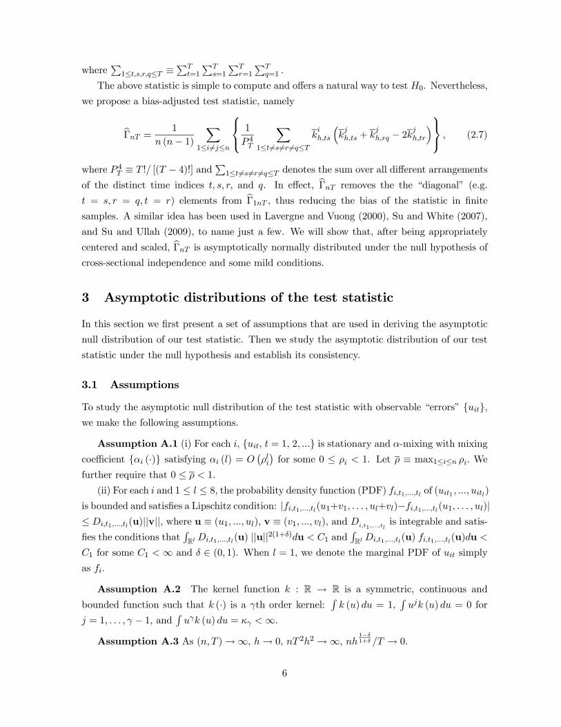
The above statistic is simple to compute and offers a natural way to test H0. Nevertheless,

we propose a bias-adjusted test statistic, namely

bΓnT = 1

n (n− 1)X

1≤i6=j≤n

⎧⎨⎩ 1

P 4T

X1≤t6=s6=r 6=q≤T

kih,ts

³kjh,ts + k

jh,rq − 2kjh,tr

´⎫⎬⎭ , (2.7)

where P 4T ≡ T !/ [(T − 4)!] andP1≤t6=s6=r 6=q≤T denotes the sum over all different arrangementsof the distinct time indices t, s, r, and q. In effect, bΓnT removes the the “diagonal” (e.g.

t = s, r = q, t = r) elements from bΓ1nT , thus reducing the bias of the statistic in finitesamples. A similar idea has been used in Lavergne and Vuong (2000), Su and White (2007),

and Su and Ullah (2009), to name just a few. We will show that, after being appropriately

centered and scaled, bΓnT is asymptotically normally distributed under the null hypothesis ofcross-sectional independence and some mild conditions.

3 Asymptotic distributions of the test statistic

In this section we first present a set of assumptions that are used in deriving the asymptotic

null distribution of our test statistic. Then we study the asymptotic distribution of our test

statistic under the null hypothesis and establish its consistency.

3.1 Assumptions

To study the asymptotic null distribution of the test statistic with observable “errors” {uit},we make the following assumptions.

Assumption A.1 (i) For each i, {uit, t = 1, 2, ...} is stationary and α-mixing with mixingcoefficient {αi (·)} satisfying αi (l) = O

¡ρli¢for some 0 ≤ ρi < 1. Let ρ ≡ max1≤i≤n ρi. We

further require that 0 ≤ ρ < 1.

(ii) For each i and 1 ≤ l ≤ 8, the probability density function (PDF) fi,t1,...,tl of (uit1 , ..., uitl)is bounded and satisfies a Lipschitz condition: |fi,t1,...,tl(u1+v1, . . . , ul+vl)−fi,t1,...,tl(u1, . . . , ul)|≤ Di,t1,...,tl(u)||v||, where u ≡ (u1, ..., ul), v ≡ (v1, ..., vl), and Di,t1,...,tl

is integrable and satis-

fies the conditions thatRRl Di,t1,...,tl(u) ||u||2(1+δ)du < C1 and

RRl Di,t1,...,tl(u) fi,t1,...,tl(u)du <

C1 for some C1 <∞ and δ ∈ (0, 1). When l = 1, we denote the marginal PDF of uit simply

as fi.

Assumption A.2 The kernel function k : R → R is a symmetric, continuous and

bounded function such that k (·) is a γth order kernel:Rk (u) du = 1,

Rujk (u) du = 0 for

j = 1, . . . , γ − 1, and R uγk (u) du = κγ <∞.Assumption A.3 As (n, T )→∞, h→ 0, nT 2h2 →∞, nh 1−δ

1+δ /T → 0.

6

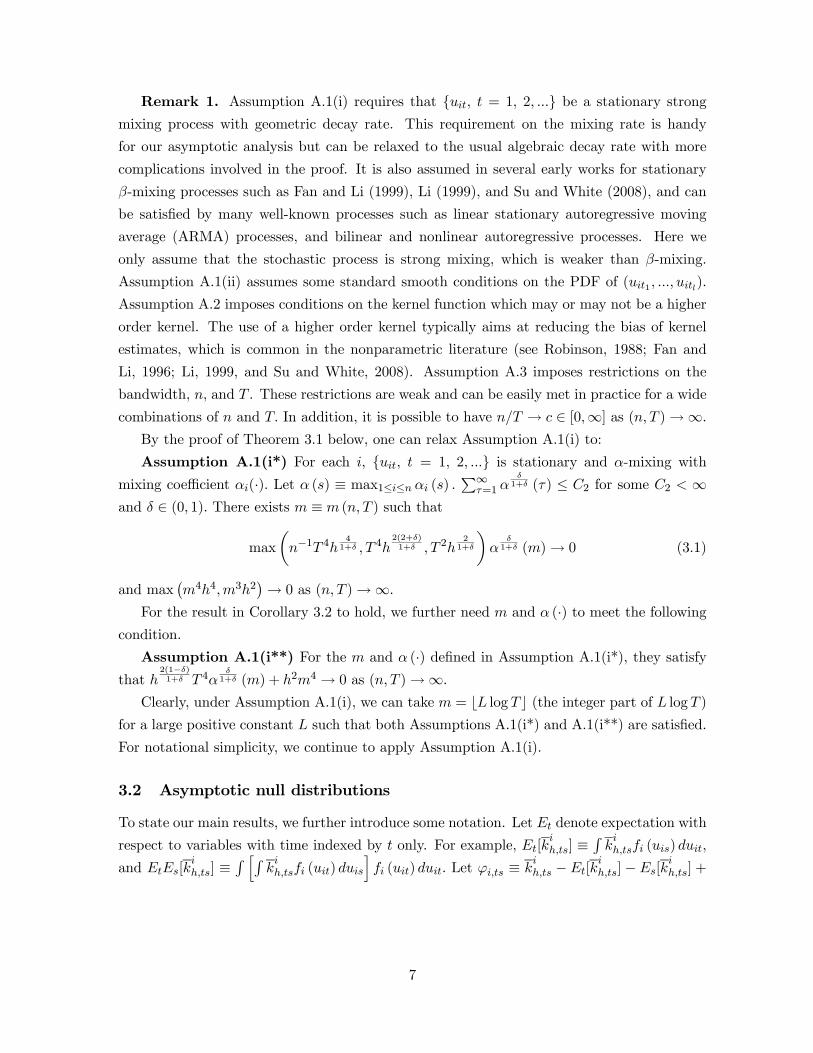
Remark 1. Assumption A.1(i) requires that {uit, t = 1, 2, ...} be a stationary strongmixing process with geometric decay rate. This requirement on the mixing rate is handy

for our asymptotic analysis but can be relaxed to the usual algebraic decay rate with more

complications involved in the proof. It is also assumed in several early works for stationary

β-mixing processes such as Fan and Li (1999), Li (1999), and Su and White (2008), and can

be satisfied by many well-known processes such as linear stationary autoregressive moving

average (ARMA) processes, and bilinear and nonlinear autoregressive processes. Here we

only assume that the stochastic process is strong mixing, which is weaker than β-mixing.

Assumption A.1(ii) assumes some standard smooth conditions on the PDF of (uit1 , ..., uitl).

Assumption A.2 imposes conditions on the kernel function which may or may not be a higher

order kernel. The use of a higher order kernel typically aims at reducing the bias of kernel

estimates, which is common in the nonparametric literature (see Robinson, 1988; Fan and

Li, 1996; Li, 1999, and Su and White, 2008). Assumption A.3 imposes restrictions on the

bandwidth, n, and T . These restrictions are weak and can be easily met in practice for a wide

combinations of n and T. In addition, it is possible to have n/T → c ∈ [0,∞] as (n, T )→∞.

By the proof of Theorem 3.1 below, one can relax Assumption A.1(i) to:

Assumption A.1(i*) For each i, {uit, t = 1, 2, ...} is stationary and α-mixing with

mixing coefficient αi(·). Let α (s) ≡ max1≤i≤n αi (s) .P∞

τ=1 αδ

1+δ (τ) ≤ C2 for some C2 < ∞and δ ∈ (0, 1). There exists m ≡ m (n, T ) such that

max

µn−1T 4h

41+δ , T 4h

2(2+δ)1+δ , T 2h

21+δ

¶α

δ1+δ (m)→ 0 (3.1)

and max¡m4h4,m3h2

¢→ 0 as (n, T )→∞.

For the result in Corollary 3.2 to hold, we further need m and α (·) to meet the followingcondition.

Assumption A.1(i**) For the m and α (·) defined in Assumption A.1(i*), they satisfythat h

2(1−δ)1+δ T 4α

δ1+δ (m) + h2m4 → 0 as (n, T )→∞.

Clearly, under Assumption A.1(i), we can take m = bL log Tc (the integer part of L logT )for a large positive constant L such that both Assumptions A.1(i*) and A.1(i**) are satisfied.

For notational simplicity, we continue to apply Assumption A.1(i).

3.2 Asymptotic null distributions

To state our main results, we further introduce some notation. Let Et denote expectation with

respect to variables with time indexed by t only. For example, Et[kih,ts] ≡

Rkih,tsfi (uis) duit,

and EtEs[kih,ts] ≡

R hRkih,tsfi (uit) duis

ifi (uit) duit. Let ϕi,ts ≡ k

ih,ts − Et[k

ih,ts] − Es[k

ih,ts] +

7

EtEs[kih,ts]. Define

1

BnT ≡ 1

n− 1X

1≤i6=j≤n

h

T − 1X

1≤t6=s≤TE£ϕi,ts

¤E£ϕj,ts

¤, and (3.2)

σ2nT ≡ 4h2

n (n− 1)X

1≤i6=j≤n

1

T (T − 1)X

1≤t6=s≤TVar

³kih,ts

´Var

³kjh,ts

´. (3.3)

We establish the asymptotic null distribution of the bΓnT test statistic in the following theorem.Theorem 3.1 Suppose Assumptions A.1-A.3 hold. Then under the null of cross-sectional

independence we have

nThbΓnT −BnTd→ N

¡0, σ20

¢as (n, T )→∞,

where σ20 ≡ lim(n,T )→∞ σ2nT .

Remark 2. The proof of Theorem 3.1 is tedious and is relegated to Appendix A. The idea

underlying the proof is simple but the details are quite involved. To see how complications

arise, let γnT,ij ≡ γnT (ui,uj) ≡ 1P 4T

P1≤t6=s6=r 6=q≤T k

ih,ts(k

jh,ts + k

jh,rq − 2kjh,tr) where ui ≡

(ui1, ..., uiT )0. Then we have bΓnT = 1

n(n−1)P1≤i6=j≤n γnT (ui,uj) . Clearly, for each pair (i, j)

with i 6= j, γnT,ij is a fourth order U -statistic along the time dimension, and by treating γnTas a kernel function, bΓnT can be regarded as a second order U -statistic along the individualdimension. To the best of our knowledge, there is no literature that treats such a two-fold

U -statistic, and it is not clear in the first sight how one should pursue in order to yield a

useful central limit theorem (CLT) for bΓnT . Even though it seems apparent for us to applythe idea of Hoeffding decomposition, how to pursue it is still challenging.

In this paper, we first apply the Hoeffding decomposition on γnT,ij for each pair (i, j) and

demonstrate that γnT,ij can be decomposed as follows

γnT,ij = 6G(2)nT,ij + 4G

(3)nT,ij +G

(4)nT,ij

where, for l = 2, 3, 4, G(l)nT,ij ≡ 1P lT

P1≤t1 6=...6=tl≤T ϑ

(l)ij (Zij,t1 , ..., Zij,tl) is an l-th order degener-

ate U -statistic with kernel ϑ(l)ij being formerly defined in Appendix A, and Zij,t ≡ (uit, ujt).Then we can obtain the corresponding decomposition for bΓnT :

bΓnT = 6G(2)nT + 4G(3)nT +G

(4)nT

where G(l)nT ≡ 1n(n−1)

P1≤i6=j≤nG

(l)nT,ij for l = 2, 3, 4. Even though for each pair (i, j) , G

(l)nT,ij

is an l-th order degenerate U -statistic with kernel ϑ(l)ij along the time dimension under H0,

1The notation can be greatly simplied under identical distributions across individuals. In this case, BnT =

n (T − 1)−1 h 1≤t 6=s≤n[E(ϕ1,ts)]2, and σ2nT = 4 [T (T − 1)]−1 h2 1≤t 6=s≤n[Var(k

1h,ts)]

2.

8

G(l)nT is by no means an l-th order degenerate U -statistic along the individual dimension under

H0. Despite this, we can conjecture as usual that the dominant term in the decomposition ofbΓnT is given by the first term 6G(2)nT , and the other two terms 4G

(3)nT and G

(4)nT are asymptot-

ically negligible. So in the second step, we make a decomposition for 6G(2)nT − 6E[G(2)nT ] and

demonstrate that

nThn6G

(2)nT − 6E[G(2)nT ]

o=

X1≤i<j≤n

wnT (ui,uj) + oP (1)

where wnT (ui,uj) ≡ 4hnT

P1≤t<s≤T ϕ

ci,tsϕ

cj,ts, and ϕ

ci,ts = ϕi,ts−E

£ϕi,ts

¤. Despite the fact that

wnT,ij ≡ wnT (ui,uj) is a non-degenerate second order U -statistic along the time dimension

any more,P1≤i<j≤nwnT (ui,uj) is a degenerate second order U -statistic along the individual

dimension. The latter enables us to apply the de Jong’s (1987) CLT for second order degener-

ate U -statistics with independent but non-identical observations. [Under the null hypothesis

of cross-sectional independence ui’s are independent across i but not identically distributed.]

The asymptotic variance ofP1≤i<j≤nwnT (ui,uj) is given by σ20 defined in Theorem 3.1 and

6nThE[G(2)nT ] delivers the asymptotic bias BnT to be corrected from the final test statistic. In

the third step, for l = 3, 4 we demonstrate nThG(l)nT = oP (1) by using the explicit formula of

ϑ(l)ij .

Remark 3. The asymptotic distribution in Theorem 3.1 is obtained by letting n and T

pass to ∞ simultaneously. Phillips and Moon (1999) introduce three approaches to handle

large dimensional panel, namely, sequential limit theory, diagonal path limit theory, and joint

limit theory, and discuss relationships between the sequential and joint limit theory. As they

remark, the joint limit theory generally requires stronger conditions to establish than the

sequential or diagonal path convergence, and by the same token, the results are also stronger

and may be expected to be relevant to a wider range of circumstances.

To implement the test, we require consistent estimates of σ2nT and BnT . Noting that

σ2nT =4h2

n (n− 1)T (T − 1)X

1≤i6=j≤n

X1≤t6=s≤T

E

∙³kih,ts

´2¸E

∙³kjh,ts

´2¸+ o (1)

=4R¡k¢2

n (n− 1)T (T − 1)X

1≤i6=j≤n

X1≤t6=s≤T

Zfi,ts (u, u) du

Zfj,ts (v, v) dv + o (1) ,

where R¡k¢ ≡ R k (u)2 du, then we can estimate σ2nT by

bσ2nT ≡ 4R¡k¢2

n (n− 1)X

1≤i6=j≤n

1

T

TXt=1

bfij,−t (uit, ujt)where bfij,−t (uit, ujt) ≡ (T−1)−1PT

s=1,s 6=t h−2 k ((uis − uit) /h) k ((ujs − ujt) /h) , i.e., bfij,−t(uit,

ujt) is the leave-one-out estimate of fij(uit, ujt). One can readily demonstrate bσ2nT is a con-9

sistent estimate of σ2nT under the null. Let

bBnT ≡ 2

T − 1TXr=2

(T − r + 1)h

n− 1X

1≤i6=j≤nbE £ϕi,1r¤ bE £ϕj,1r¤ ,

where bE £ϕi,1r¤ ≡ (T − r + 1)−1PT−r+1

t=1 kih,t,t+r−1 − T−1 (T − 1)−1P1≤t6=s≤T k

ih,ts. We es-

tablish the consistency of bBnT for BnT in Appendix B. Then we can define a feasible test

statistic: bInT = nThbΓnT − bBnTbσnT ,

which is asymptotically distributed as standard normal under the null. We can compare bInT tothe one-sided critical value zα, the upper α percentile from the standard normal distribution,

and reject the null if bInT > zα. The following corollary formally establishes the asymptotic

normal distribution of bInT under H0

Corollary 3.2 Suppose the conditions in Theorem 3.1 hold. Then we have

bInT d→ N (0, 1) as (n, T )→∞.

3.3 Consistency

To study the consistency of our test, we consider the nontrivial case where μA ≡ limn→∞ Γn >

0, where

Γn ≡ 1

n (n− 1)X

1≤i6=j≤n

Z Z[fij (u, v)− fi (u) fj (v)]

2 dudv.

We need to add the following assumption that takes into account cross-sectional depen-

dence under the alternative.

Assumption A.4 For each pair (i, j) with i 6= j, the joint PDF fij of uit and ujt is bounded

and satisfies a Lipschitz condition: |fij(u1+v1, u2+v2)−fij(u1, u2)| ≤ Dij(u1, u2)|| (v1, v2) ||,and Dij is integrable uniformly in (i, j):

R RDij(u, v) fij(u, v)dudv < C3 for some C3 <∞.

The following theorem establishes the consistency of the test.

Theorem 3.3 Suppose Assumptions A.1-A.4 hold and μA > 0. Then under H1, P³bInT > dnT

´→ 1 for any sequence dnT = oP (nTh) as (n, T )→∞.

Remark 4. Theorem 3.3 indicates that under H1 our test statistic bInT explodes at therate nTh provided μA > 0. This can occur if fij (u, v) and fi (u) fj (v) differ on a set of positive

measure for a “large” number of pairs (i, j) where the number explodes to the infinity at rate

n2. It rules out the case where they differ on a set of positive measure only for a finite fixed

number of pairs, or the case where the number of pairwise joint PDFs that differ from the

10

product of the corresponding marginal PDFs on a set of positive measure is diverging to

infinity as n → ∞ but at a slower rate than n2. In either case, our test statistic bInT cannotexplode to the infinity at the rate nTh, but can still be consistent. Specifically, as long as

λnTΓn → μA and λnT/ (nTh) → 0 as (n, T ) → ∞ for some diverging sequence {λnT} , ourtest is still consistent as bInT now diverges to infinite at rate (nTh) /λnT .

Remark 5. We have not studied the asymptotic local power property of our test. Unlike

the CGL’s test for cross-sectional uncorrelation, it is difficult for us to set up a desirable

sequence of Pitman local alternatives that converge to the null at a certain rate and yet

enable us to obtain the nontrivial asymptotic power property of our test. Once we deviate

from the null hypothesis, all kinds of cross-sectional dependence can arise in the data, which

makes the analysis complicated and challenging. See also the remarks in Section 6.

4 Tests based on residuals from nonparametric regressions

In this section, we consider tests for cross-sectional dependence among the unobservable error

terms in the nonparametric panel data model (2.1). We must estimate the error terms from

the data before conducting the test.

We assume that the regression functions gi (·), i = 1, . . . , n, are sufficiently smooth, andconsider estimating them by the pth order local polynomial method (p = 1, 2, 3 in most

applications). See Fan and Gijbels (1996) and Li and Racine (2007) for the advantage of

local polynomial estimates over the local constant (Nadaraya-Watson) estimates. If gi (·) hasderivatives up to the pth order at a point x, then for any Xit in a neighborhood of x, we have

gi(Xit) = gi(x) +X

1≤|j|≤p

1

j!D|j|gi (x) (Xit − x)j + o (kXit − xkp)

≡X

0≤|j|≤pβi,j (x; b) ((Xit − x)/b)j + o (kXit − xkp) .

Here, we use the notation of Masry (1996a, 1996b): j = (j1, ..., jd), |j| =Pd

a=1 ja, xj =

Πda=1x

jaa ,P0≤|j|≤p =

Ppl=0

Plj1=0

...Pl

jd=0j1+...+jd=l

, D|j|gi (x) =∂|j|gi(x)

∂j1x1...∂jdxd, βi,j (x; b) =

b|j|j! D

|j|gi (x) ,

where j! ≡ Πda=1ja! and b ≡ b (n, T ) is a bandwidth parameter that controls how “close” Xit

is from x. With observations {(yit,Xit)}Tt=1 , we consider choosing βi, the stack of βi,j in a

lexicographical order, to minimize the following criterion function

QT (x;βi) ≡ T−1TXt=1

⎛⎝yit −X

0≤|j|≤pβj((Xit − x)/b)j

⎞⎠2wb (Xit − x) , (4.1)

where wb (x) = b−dw (x/b) , and w is a symmetric PDF on Rd. The pth order local polynomial

estimate of gi(x) is then defined as the minimizing concept in the above minimization problem.

11

Let Nl ≡ (l+d−1)!/(l!(d−1)!) be the number of distinct d-tuples j with |j| = l. It denotes

the number of distinct l-th order partial derivatives of gi(x) with respect to x. Arrange the

Nl d-tuples as a sequence in the lexicographical order (with highest priority to last position),

so that φl(1) ≡ (0, 0, ..., l) is the first element in the sequence and φl(Nl) ≡ (l, 0, ..., 0) is thelast element, and let φ−1l denote the mapping inverse to φl. Let N ≡

Ppl=0Nl. Define SiT (x)

andWiT (x) as a symmetric N ×N matrix and an N × 1 vector, respectively:

SiT (x) ≡

⎡⎢⎢⎢⎢⎢⎣SiT,0,0 (x) SiT,0,1 (x) · · · SiT,0,p (x)

SiT,1,0 (x) SiT,1,1 (x) · · · SiT,1,p (x)...

.... . .

...

SiT,p,0 (x) SiT,p,1 (x) · · · SiT,p,p (x)

⎤⎥⎥⎥⎥⎥⎦ , WiT (x) ≡

⎡⎢⎢⎢⎢⎣WiT,0(x)

WiT,1(x)

:

WiT,p(x)

⎤⎥⎥⎥⎥⎦where SiT,j,k(x) is an Nj ×Nk submatrix with the (l, r) element given by

[SiT,j,k(x)]l,r ≡1

T

TXt=1

µXit − x

b

¶φj(l)+φk(r)

wb (Xit − x) ,

andWiT,j(x) is an Nj ×1 subvector whose r-th element is given by

[WiT,j(x)]r ≡1

T

TXt=1

yit

µXit − x

b

¶φj(r)

wb (Xit − x) .

Then we can denote the pth order local polynomial estimate of gi(x) as

egi(x) ≡ e01 [SiT (x)]−1WiT (x)

where e1 ≡ (1, 0, · · · , 0)0 is an N × 1 vector.For each j with 0 ≤ |j| ≤ 2p, let μj ≡

RRd x

jw(x)dx. Define the N ×N dimensional matrix

S by

S ≡

⎡⎢⎢⎢⎢⎢⎣S0,0 S0,1 ... S0,pS1,0 S1,1 ... S1,p...

.... . .

...

Sp,0 Sp,1 ... Sp,p

⎤⎥⎥⎥⎥⎥⎦ , (4.2)

where Si,j is an Ni×Nj dimensional matrix whose (l, r) element is μφi(l)+φj(r). Note that the

elements of the matrix S are simply multivariate moments of the kernel w. For example, ifp = 1, then

S =

" Rw (x) dx

Rx0w (x) dxR

xw (x) dxRxx0w (x) dx

#=

"1 01×d0d×1

Rxx0w (x) dx

#,

where 0a×c is an a× c matrix of zeros.

12

Let euit ≡ yit − egi (Xit) for i = 1, . . . , n and t = 1, . . . , T . Define eΓnT , eBnT , and eσ2nTanalogously to bΓnT , bBnT , bσ2nT but with {uit} being replaced by {euit}. Then we can considerthe following “feasible” test statistic

eInT ≡ nTheΓnT − eBnTeσnT .

To demonstrate the asymptotic equivalence of eInT and bInT , we add the following assumptions.Assumption A.5 (i) For each i = 1, . . . , n, {Xit, t = 1, 2, ...} is stationary and α-mixing

with mixing coefficient {ai (·)} satisfyingP∞

j=1 jκ0a (j)δ0/(2+δ0) < C4 for some C4 < ∞,

κ0 > δ0/(2 + δ0), and δ0 > 0, where a (j) ≡ max1≤i≤n ai (j) .(ii) For each i = 1, . . . , n, the support Xi of Xit is compact on Rd. The PDF pi of

Xit exists, is Lipschitz continuous, and is bounded away from zero on Xi uniformly ini : min1≤i≤n infxi∈Xi pi (xi) > C5 for some C5 > 0. The joint PDF of Xit and Xis is uni-

formly bounded for all t 6= s by a constant that does not depend on i or |t− s| .(iii) {uit, i = 1, 2, . . . , t = 1, 2, . . .} is independent of {Xit, i = 1, 2, . . . , t = 1, 2, . . .} .Assumption A.6 (i) For each i = 1, . . . , n, the individual regression function gi(·), is

p+ 1 times continuously partially differentiable.

(ii) The (p+ 1)-th order partial derivatives of gi are Lipschitz continuous on Xi.Assumption A.7 (i) The kernel function w : Rd → R+ is a continuous, bounded, and

symmetric PDF; S is positive definite (p.d.).(ii) Let w (x) ≡ kxk2(2+δ0)pw (x) . w is integrable with respect to the Lebesgue measure.

(iii) Let Wj(x) ≡ xjw(x) for all d-tuples j with 0 ≤ |j| ≤ 2p + 1. Wj(x) is Lipschitz

continuous for 0 ≤ |j| ≤ 2p + 1. For some C6 < ∞ and C7 < ∞, either w (·) is compactlysupported such that w (x) = 0 for kxk > C6, and ||Wj(x) −Wj(ex)|| ≤ C7 ||x− ex|| for any x,ex ∈ Rd and for all j with 0 ≤ |j| ≤ 2p + 1; or w(·) is differentiable, k∂Wj(x)/∂xk ≤ C6, and

for some ι0 > 1, |∂Wj(x)/∂x| ≤ C6 kxk−ι0 for all kxk > C7 and for all j with 0 ≤ |j| ≤ 2p+1.Assumption A.8 (i) The kernel function k is second order differentiable with first order

derivative k0 and second order derivative k00. Both uk (u) and uk0 (u) tend to 0 as |u| → ∞.

(ii) For some ck <∞ and Ak <∞, |k00 (u) | ≤ ck and for some γ0 > 1, |k00 (u) | ≤ ck |u|−γ0 forall |u| > Ak.

Assumption A.9 (i) Let η ≡ T−1b−d+b2(p+1). As (n, T )→∞, Th5 →∞, T 3/2bdh5 →∞,

and nTh(η2 + h−4η3 + h−8η4)→ 0.

(ii) For the m defined in Assumption A.1(i*), max(nhmb2(p+1), nmT−1b−d, n2T−4m6h−2,n2m2h−2b4(p+1), nhm2/T, nh−3m3/T 2, m3/T )→ 0.

Remark 6 Assumptions A.5 (i)-(ii) are subsets of some standard conditions to obtain

the uniform convergence of local polynomial regression estimates. Like CGL, we assume the

13

independence of {uit} and {Xjs} for all i, j, t, s in Assumptions A.5(iii), which will greatlyfacilitate our asymptotic analysis. Assumptions A.6 and A.7 are standard in the literature on

local polynomial estimation. In particular, following Hansen (2008), the compact support of

the kernel function w in Masry (1996b) can be relaxed as in Assumption A.7(iii). Assumption

A.8 specifies more conditions on the kernel function k used in the estimation of joint and

marginal densities of the error terms. They are needed because we need to apply Taylor

expansions on functions associated with k. Assumption A.9 imposes further conditions on

h, n, and T and their interaction with the smoothing parameter b and the order p of local

polynomial used in the local polynomial estimation. If we relax the geometric α-mixing rate

in Assumption A.1(i) to the algebraic rate, then we need to add the following condition on

the bandwidth parameters, sample sizes, and the choices of m and p :

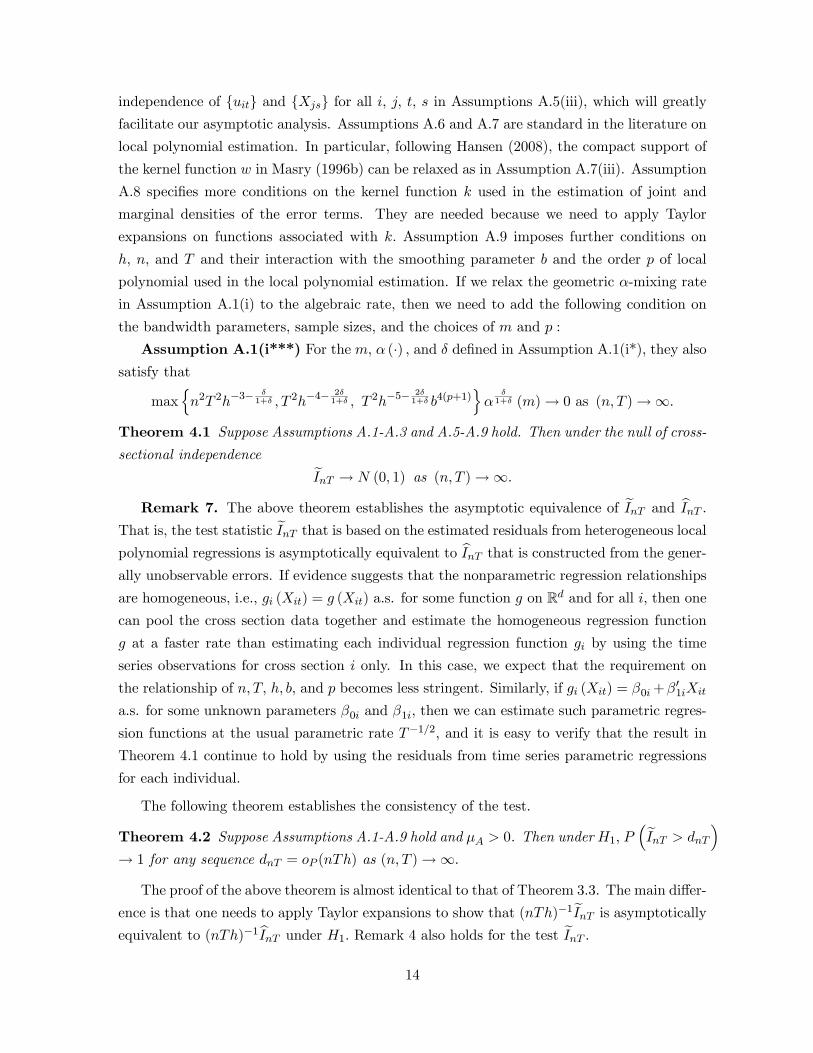
Assumption A.1(i***) For the m, α (·) , and δ defined in Assumption A.1(i*), they alsosatisfy that

maxnn2T 2h−3−

δ1+δ , T 2h−4−

2δ1+δ , T 2h−5−

2δ1+δ b4(p+1)

oα

δ1+δ (m)→ 0 as (n, T )→∞.

Theorem 4.1 Suppose Assumptions A.1-A.3 and A.5-A.9 hold. Then under the null of cross-

sectional independence eInT → N (0, 1) as (n, T )→∞.

Remark 7. The above theorem establishes the asymptotic equivalence of eInT and bInT .That is, the test statistic eInT that is based on the estimated residuals from heterogeneous localpolynomial regressions is asymptotically equivalent to bInT that is constructed from the gener-ally unobservable errors. If evidence suggests that the nonparametric regression relationships

are homogeneous, i.e., gi (Xit) = g (Xit) a.s. for some function g on Rd and for all i, then one

can pool the cross section data together and estimate the homogeneous regression function

g at a faster rate than estimating each individual regression function gi by using the time

series observations for cross section i only. In this case, we expect that the requirement on

the relationship of n, T, h, b, and p becomes less stringent. Similarly, if gi (Xit) = β0i+β01iXit

a.s. for some unknown parameters β0i and β1i, then we can estimate such parametric regres-

sion functions at the usual parametric rate T−1/2, and it is easy to verify that the result inTheorem 4.1 continue to hold by using the residuals from time series parametric regressions

for each individual.

The following theorem establishes the consistency of the test.

Theorem 4.2 Suppose Assumptions A.1-A.9 hold and μA > 0. Then under H1, P³eInT > dnT

´→ 1 for any sequence dnT = oP (nTh) as (n, T )→∞.

The proof of the above theorem is almost identical to that of Theorem 3.3. The main differ-

ence is that one needs to apply Taylor expansions to show that (nTh)−1eInT is asymptoticallyequivalent to (nTh)−1bInT under H1. Remark 4 also holds for the test eInT .

14

5 Monte Carlo simulations

In this section, we conduct a small set of Monte Carlo simulations to evaluate the finite sample

performance of our test and compare it with Pesaran’s and CGL’s tests for cross-sectional

uncorrelation.

5.1 Data generating processes

We consider the following six data generating processes (DGPs) in our Monte Carlo study.

DGPs 1-2 are for size study, and DGPs 3-6 are for power comparisons.

DGP 1:

yit = αi + βiXit + uit,

where across both i and t, Xit ∼ IID U (−3, 3), αi ∼IID U(0, 1), βi ∼ IID N (0, 1), and they

are mutually independent of each other.

DGP 2:

yit = (1 + θi) exp(Xit)/(1 + exp(Xit)) + uit,

where across both i and t, Xit ∼ IID U (−3, 3) , θi ∼ IID N (0, 0.25), and they are mutually

independent of each other.

In DGPs 1-2, we consider two kinds of error terms: (i) uit ∼ IID N (0, 1) across both i

and t and independent of {αi, βi,Xit}; and (ii) {uit} is IID across i and an AR(1) process

over t: uit = 0.5ui,t−1 + εit, where εit ∼ IID N (0, 0.75) across both i and t and independent

of {αi, βi,Xit}. Clearly, there is no cross-sectional dependence in either case.In terms of conditional mean specification, DGPs 3 and 5 are identical to DGP 1, and

DGPs 4 and 6 are identical to DGP2. The only difference lies in the specification of the error

term uit. In DGPs 3-4, we consider the following single-factor error structure:

uit = 0.5λiFt + εit (5.1)

where the factors Ft are IID N (0, 1) , and the factor loadings λi are IID N (0, 1) and indepen-

dent of {Ft} .We consider two configurations for εit : (i) εit are IID N (0, 1) and independent

of {Ft, λi}, and (ii) εit = 0.5εit−1 + ηit where ηit are IID N (0, 0.75) across both i and t, and

independent of {Ft, λi}.In DGPs 5-6, we consider the following two-factor error structure:

uit = 0.3λ1iF1t + 0.3λ2iF2t + εit (5.2)

where both factors F1t and F2t are IID N (0, 1) , λ1i are IID N (0, 1) , λ2i are IID N (0.5, 1) ,

F1t, F2t, λ1i, and λ2i are mutually independent of each other, and the error process {εit} isspecified as in DGPs 3-4 with two configurations.

15

5.2 Bootstrap

It is well known that the asymptotic normal distribution typically cannot approximate well

the finite sample distribution of many nonparametric test statistics under the null hypothesis.

In fact, the empirical level of these tests can be sensitive to the choice of bandwidths or highly

distorted in finite samples. So we suggest using a bootstrap method to obtain the bootstrap

p-values. Note that we need to estimate E (ϕts) in BnT , and that the dependence structure in

each individual error process {uit}Tt=1 will affect the asymptotic distribution of our test underthe null. Like Hsiao and Li (2001), we need to mimic the dependence structure over time.

So we propose to apply the stationary bootstrap procedure of Politis and Romano (1994) to

each individual i’s residual series {euit}Tt=1 . The procedure goes as follows:1. Obtain the local polynomial regression residuals euit = Yit − egi (xit) for each i and t.

2. For each i, obtain the bootstrap time series sequence {u∗it}Tt=1 by the method of station-ary bootstrap. 2

3. Calculate the bootstrap test statistic eI∗nT = (nTheΓ∗nT − eB∗nT )/eσ∗nT , where eΓ∗nT , eB∗nT andeσ∗nT are defined analogously to eΓnT , eBnT and eσnT but with euit be replaced by u∗it.4. Repeat steps 1-3 for B times and index the bootstrap statistics as {eI∗nT,j}Bj=1. Calculatethe bootstrap p-value p∗ ≡ B−1

PBj=1 1(

eI∗nT,j > eInT ) where 1(·) is the usual indicatorfunction, and reject the null hypothesis of cross-sectional independence if p∗ is smallerthan the prescribed level of significance.

Note that we have imposed the null restriction of cross-sectional independence implicitly

because we generate {u∗it} independently across all individuals. We conjecture that for suf-ficiently large B, the empirical distribution of {eI∗nT,j}Bj=1 is able to approximate the finitesample distribution of eInT under the null hypothesis, but are not sure whether this can haveany improvement over the asymptotic normal approximation. The theoretical justification for

the validity of our bootstrap procedure goes beyond the scope of this paper.

5.3 Test results

We consider three tests of cross-sectional dependence in this section: Pesaran’s CD test for

cross-sectional dependence, CGL test for cross-sectional uncorrelation, and the eInT test pro-2A simple description of the resampling algorithm goes as follows. Let p be a fixed number in (0, 1).

Let u∗i1 be picked at random from the original T residuals {ui1, ..., uiT }, so that u∗i1 = uiT1 , say, for some

T1 ∈ {1, ..., T}. With probability p, let u∗i2 be picked at random from the original T residuals {ui1, ..., uiT };with probability 1 − p, let u∗i2 = ui,T1+1 so that u

∗i2 would be the “next” observation in the original residual

series following uiT1 . In general, given that u∗it is determined by the Jth observation uiJ in the original residual

series, let u∗i,t+1 be equal to ui,J+1 with probability 1−p and be picked at random from the original T residuals

with probability p. We set p = T−1/3 in the simulations.

16

Table 1: Finite sample rejection frequency for DGPs 1-2 (size study, nomial level 0.05)

DGP n T (i) uit ∼ IID N (0, 1) (ii) uit = 0.5ui,t−1 + εitP CGL SZ P CGL SZ

1 25 25 0.040 0.044 0.054 0.092 0.060 0.08250 0.060 0.044 0.048 0.130 0.062 0.082100 0.056 0.058 0.064 0.126 0.080 0.066

50 25 0.060 0.044 0.062 0.118 0.066 0.12850 0.070 0.052 0.080 0.112 0.076 0.074100 0.034 0.030 0.048 0.124 0.066 0.064

2 25 25 0.038 0.044 0.052 0.088 0.050 0.09050 0.056 0.062 0.060 0.122 0.062 0.082100 0.058 0.044 0.064 0.128 0.068 0.070

50 25 0.054 0.042 0.058 0.076 0.078 0.12050 0.064 0.060 0.060 0.110 0.050 0.084100 0.038 0.052 0.052 0.108 0.068 0.060

Note: P, CGL, and SZ refer to Pesaran’s, CGL’s and our tests, respectively.

posed in this paper. To conduct our test, we need to choose kernels and bandwidths. To

estimate the heterogeneous regression functions, we conduct a third-order local polynomial

regression (p = 3) by choosing the second order Gaussian kernel and rule-of-thumb bandwidth:

b = sXT−1/9 where sX denotes the sample standard deviation of {Xit} across i and t. To es-

timate the marginal and pairwise joint densities, we choose the second order Gaussian kernel

and rule-of-thumb bandwidth h = suT−1/6, where su denotes the sample standard deviation

of {euit} across i and t. For the CGL test, we follow their paper and consider a local linear re-gression to estimate the conditional mean function by using the Gaussian kernel and choosing

the bandwidth through the leave-one-out cross-validation method. For the Pesaran’s test, we

estimate the heterogeneous regression functions by using the linear model, and conduct his

CD test based on the parametric residuals.

For all tests, we consider n = 25, 50, and T = 25, 50, 100. For each combination of n and

T, we use 500 replications for the level and power study, and 200 bootstrap resamples in each

replication.

Table 1 reports the finite sample level for Pesaran’s CD test, the CGL test and our test

(denoted as P, CGL, and SZ, respectively in the table). When the error terms uit are IID

across t, all three tests perform reasonably well for all combinations of n and T and both DGPs

under investigation in that the empirical levels are close to the nominal level. When {uit}follows an AR(1) process along the time dimension, we find out the CGL test outperforms

the Pesaran’s test in terms of level performance: the latter test tends to have a large size

17

distortion which does not improve when either n or T increases. In contrast, our test can be

oversized when n/T is not small (e.g., n = 50 and T = 25) so that the parameter estimation

error plays a non-negligible role in the finite samples, but the level of our test improves quickly

as T increases for fixed n.

Table 2 reports the finite sample power performance of all three tests for DGPs 3-6. For

DGPs 3-4, we have a single-factor error structure. Noting that the factor loadings λi have zero

mean in our setup, neither Pesaran’s nor CGL’s test has power in detecting cross-sectional

dependence in this case. This is confirmed by our simulations. In contrast, our tests have

power in detecting deviations from cross-sectional dependence. As either n or T increases,

the power of our test increases. DGPs 5-6 exhibit a two-factor error structure where one of

the two sequences of factor loadings have nonzero mean, and all three tests have power in

detecting cross-sectional dependence. As either n or T increases, the powers of all three tests

increase quickly and our test tends to more powerful than the Pesaran’s and CGL’s tests.

6 Concluding remarks

In this paper, we propose a nonparametric test for cross-sectional dependence in large di-

mensional panel. Our tests can be applied to both raw data and residuals from heterogenous

nonparametric (or parametric) regressions. The requirement on the relative magnitude of n

and T is quite weak in the former case, and very strong in the latter case in order to con-

trol the asymptotic effect of the parameter estimation error on the test statistic. In both

cases, we establish the asymptotic normality of our test statistic under the null hypothesis of

cross-sectional independence. The global consistency of our test is also established. Monte

Carlo simulations indicate our test performs reasonably well in finite samples and has power

in detecting cross-sectional dependence when the Pesaran’s and CGL’s tests fail.

We have not pursued the asymptotic local power analysis for our nonparametric test in

this paper. It is well known that the study of asymptotic local power is rather difficult

in nonparametric testing for serial dependence, see Tjøstheim (1996) and Hong and White

(2005). Similar remark holds true for nonparametric testing for cross-sectional dependence.

To analyze the local power of their test, Hong and White (2005) consider a class of locally

j-dependent processes for which there exists serial dependence at lag j only, but j may grow

to infinity as the sample size passes to infinity. It is not clear whether one can extend their

analysis to our framework since there is no natural ordering along the individual dimensions

in panel data models. In addition, it may not be advisable to consider a class of panel data

models for which there exists cross-sectional dependence at pairwise level only: if any two of

uit, ujt, and ukt (i 6= j 6= k) are dependent, they tend to be dependent on the other one also.

Thus we conjecture that it is very challenging to conduct the asymptotic local power analysis

for our nonparametric test.

18

Table 2: Finite sample rejection frequency for DGPs 3-6 (power study, nomial level 0.05)

DGP n T (i) εit ∼ IID N (0, 1) (ii) εit = 0.5εit−1 + ηitP CGL SZ P CGL SZ

3 25 25 0.040 0.046 0.446 0.092 0.052 0.59050 0.060 0.058 0.778 0.130 0.060 0.860100 0.056 0.074 0.950 0.126 0.038 0.984

50 25 0.060 0.040 0.772 0.118 0.070 0.86650 0.070 0.060 0.972 0.112 0.074 0.992100 0.034 0.064 0.998 0.124 0.068 1.000

4 25 25 0.038 0.074 0.446 0.098 0.044 0.61650 0.056 0.052 0.772 0.206 0.066 0.858100 0.058 0.062 0.954 0.234 0.044 0.984

50 25 0.054 0.046 0.772 0.148 0.086 0.87050 0.064 0.068 0.970 0.190 0.072 0.990100 0.038 0.062 0.998 0.270 0.068 1.000

5 25 25 0.326 0.248 0.208 0.410 0.304 0.41850 0.412 0.332 0.444 0.486 0.350 0.672100 0.584 0.446 0.740 0.594 0.424 0.910

50 25 0.550 0.442 0.456 0.626 0.508 0.68050 0.720 0.620 0.812 0.754 0.640 0.918100 0.842 0.742 0.988 0.888 0.776 0.996

6 25 25 0.304 0.232 0.250 0.420 0.292 0.40650 0.428 0.330 0.424 0.488 0.348 0.634100 0.568 0.426 0.762 0.588 0.402 0.908

50 25 0.548 0.454 0.424 0.624 0.516 0.66250 0.724 0.636 0.814 0.760 0.636 0.908100 0.838 0.746 0.980 0.888 0.794 1.000

Note: P, CGL, and SZ refer to Pesaran’s, CGL’s and our tests, respectively.

19

APPENDIX

Throughout this appendix, we use C to signify a generic constant whose exact value may vary

from case to case. Recall P lT ≡ T !/(T − l)! and Cl

T ≡ T !/ [(T − l)!l!] for integers l ≤ T .

A Proof of Theorem 3.1

Recall ϕi,ts ≡ ki

h,ts−Et[ki

h,ts]−Es[ki

h,ts]+EtEs[ki

h,ts] where ki

h,ts ≡ kh (uit − uis) andEs denotes expec-

tation taken only with respect to variables indexed by time s, that is, Es(ki

h,ts) ≡Rkh (uit − u) fi (u) du.

Let ci,ts ≡ E(ϕi,ts), and cts ≡ (n− 1)−1Pn

i=1 ci,ts. We will frequently use the fact that for t 6= s,

ci,ts ≤ Ch−δ

1+δαδ

1+δ

i (|t− s|) (A.1)

as by the law of iterated expectations, the triangle inequality, and Lemma E.2, we have |ci,ts|= |E[kih,ts]−EtEs[k

i

h,ts]| = |E{E[ki

h,ts|uit]−Es[ki

h,ts]}| ≤ E|E[kih,ts|uit]−Es[ki

h,ts]| ≤ Ch−δ

1+δαδ

1+δ

i (|t− s|) . Letα (j) ≡ max1≤i≤n αi (j) . Let m ≡ bL log T c (the integer part of L log T ) where L is a large positiveconstant so that the conditions on m in Assumption A.1(i*) are all met by Assumption A.1(i). In

addition, it is obvious thatP∞

τ=1 αδ

1+δ (τ) = O (1) under Assumption A.1(i).

Let Zij,t ≡ (uit, ujt) and ςij,tsrq ≡ ς (Zij,t, Zij,s, Zij,r, Zij,q) = ki

h,ts(kj

h,ts + kj

h,rq − 2kj

h,tr). Letςij,tsrq ≡ ς (Zij,t, Zij,s, Zij,r, Zij,q) ≡ 1

4!

P4! ςij,tsrq, where

P4! denotes summation over all 4! different

permutations of (t, s, r, q). That is, ςij,tsrq is a symmetric version of ςij,tsrq by symmetrizing over thefour time indices and it is easy to verify that

ς̄ij,tsrq =1

12{kih,ts(2k

j

h,ts + 2kj

h,rq − kj

h,tr − kj

h,sr − kj

h,tq − kj

h,sq)

+ki

h,tr(2kj

h,tr + 2kj

h,qs − kj

h,ts − kj

h,sr − kj

h,tq − kj

h,rq)

+ki

h,tq(2kj

h,tq + 2kj

h,sr − kj

h,tr − kj

h,qr − kj

h,ts − kj

h,sq)

+ki

h,sr(2kj

h,sr + 2kj

h,qt − kj

h,st − kj

h,rt − kj

h,sq − kj

h,rq)

+ki

h,sq(2kj

h,sq + 2kj

h,rt − kj

h,st − kj

h,qt − kj

h,sr − kj

h,qr)

+ki

h,rq(2kj

h,rq + 2kj

h,st − kj

h,rt − kj

h,qt − kj

h,rs − kj

h,qs)}. (A.2)

Then we can write bΓnT asbΓnT =

1

n (n− 1)X

1≤i6=j≤n

1

P 4T

X1≤t6=s6=r 6=q≤T

ςij,tsrq

=1

n (n− 1)X

1≤i6=j≤n

1

C4T

X1≤t1<t2<t3<t4≤T

ςij,t1t2t3t4 . (A.3)

Let θij = E1E2E3E4 [ς (Zij,1, Zij,2, Zij,3, Zij,4)] and ς̄ij,c (z1, . . . , zc) = Ec+1 · · ·E4[ς̄(z1, . . . , zc,Zij,c+1, . . . , Zij,4)] for nonrandom z1, . . . , zc and c = 1, 2, 3, 4. Let ϑ

(1)ij (z1) = ς̄ij,1 (z1) − θij and

ϑ(c)ij (z1, . . . , zc) = ς̄ij,c (z1, . . . , zc) −

Pc−1k=1

P(c,k) ϑ

(k)ij (zt1 , . . . , ztk) − θij for c = 2, 3, 4, where the sumP

(c,k) is taken over all subsets 1 ≤ t1 < · · · < tk ≤ c of {1, 2, . . . , c} . It is easy to verify that θij = 0,ϑ(1)ij (Zij,t) = 0, and

ϑ(2)ij (Zij,t, Zij,s) = ς̄ij,2 (Zij,t, Zij,s) =

1

6ϕi,tsϕj,ts. (A.4)

20

Similarly, straightforward but tedious calculations show that

ϑ(3)ij (Zij,t, Zij,s, Zij,r)

= ς̄ij,3 (Zij,t, Zij,s, Zij,r)− ς̄ij,2 (Zij,t, Zij,s)− ς̄ij,2 (Zij,t, Zij,r)− ς̄ij,2 (Zij,s, Zij,r)

= − 112

£ϕi,ts

¡ϕj,tr + ϕj,sr

¢+ ϕi,tr

¡ϕj,ts + ϕj,sr

¢+ ϕi,sr

¡ϕj,st + ϕj,rt

¢¤(A.5)

and

ϑ(4)ij (Zij,t, Zij,s, Zij,r, Zij,q)

= ς (Zij,t, Zij,s, Zij,r, Zij,q)− ς̄ij,2 (Zij,t, Zij,s)− ς̄ij,2 (Zij,t, Zij,r)− ς̄ij,2 (Zij,t, Zij,q)

−ς̄ij,2 (Zij,s, Zij,r)− ς̄ij,2 (Zij,s, Zij,q)− ς̄ij,2 (Zij,r, Zij,q)− ς̄ij,3 (Zij,t, Zij,s, Zij,r)

−ς̄ij,3 (Zij,t, Zij,s, Zij,q)− ς̄ij,3 (Zij,t, Zij,r, Zij,q)− ς̄ij,3 (Zij,s, Zij,r, Zij,q)

=1

6

©ϕi,tsϕj,rq + ϕi,trϕj,sq + ϕi,rqϕj,ts + ϕi,sqϕj,tr + ϕi,tqϕj,sr + ϕi,srϕj,tq

ª, (A.6)

where (A.5) and (A.6) will be needed in the proofs of Propositions A.4 and A.5, respectively.Let G(k)nT ≡ 1

n(n−1)PkT

P1≤i6=j≤n

P(T,k) ϑ

(k)ij (Zij,t1 , . . . , Zij,tk) for k = 1, 2, 3, 4, where

P(T,k) de-

notes summation over all P kT permutations (t1, ..., tk) of distinct integers chosen from {1, 2, ..., T} (See

Lee (1990), Ch 1). Then by the Hoeffding decomposition, we have

bΓnT = 6G(2)nT + 4G(3)nT +G

(4)nT . (A.7)

Let ΓnT ≡ 6G(2)nT . Noting that nThE(ΓnT ) =

2h(n−1)(T−1)

P1≤i6=j≤n

P1≤t<s≤T E

£ϕi,tsϕj,ts

¤= BnT

underH0, we complete the proof of the theorem by showing that: (i) nTh[ΓnT−E¡ΓnT

¢]d→ N

¡0, σ20

¢,

(ii) nThG(3)nT = oP (1) , and (iii) nThG

(4)nT = oP (1) . These results are established respectively in

Propositions A.1, A.4, and A.5 below.

Proposition A.1 nTh£ΓnT −E

¡ΓnT

¢¤ d→ N¡0, σ20

¢.

Proof. Let ϕci,ts ≡ ϕi,ts −E(ϕi,ts). Then we have ΓnT −E(ΓnT ) = ΓnT,1 + ΓnT,2, where

ΓnT,1 ≡ 2

n (n− 1)X

1≤i<j≤n

1

C2T

X1≤t<s≤T

ϕci,tsϕcj,ts, and

ΓnT,2 ≡ 1

n (n− 1)X

1≤i6=j≤n

1

C2T

X1≤t<s≤T

©ϕci,tsE

£ϕj,ts

¤+ ϕcj,tsE

£ϕi,ts

¤ª.

We prove the proposition by showing that

nThΓnT,1 =nT

(n− 1) (T − 1)WnTd→ N

¡0, σ20

¢, (A.8)

andnThΓnT,2 = oP (1) , (A.9)

where WnT ≡P

1≤i<j≤nwij , wij ≡ wnT,ij ≡ wnT (ui,uj) ≡ 4hnT

P1≤t<s≤T ϕci,tsϕ

cj,ts, and ui ≡

(ui1, ...., uiT )0. Noting that nT/[(n − 1)(T − 1)] → 1, the proof is completed by Lemmas A.2-A.3

below.

21

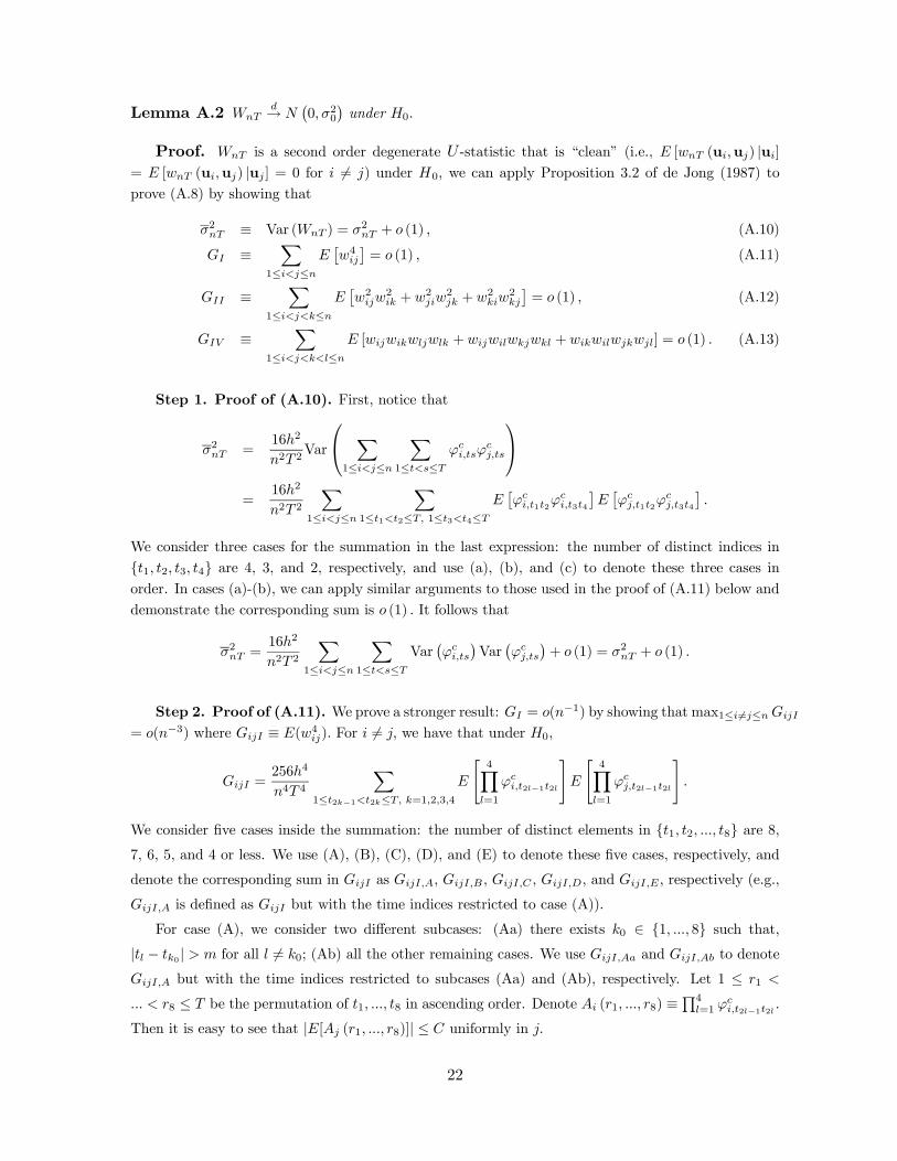
Lemma A.2 WnTd→ N

¡0, σ20

¢under H0.

Proof. WnT is a second order degenerate U -statistic that is “clean” (i.e., E [wnT (ui,uj) |ui]= E [wnT (ui,uj) |uj ] = 0 for i 6= j) under H0, we can apply Proposition 3.2 of de Jong (1987) toprove (A.8) by showing that

σ2nT ≡ Var (WnT ) = σ2nT + o (1) , (A.10)

GI ≡X

1≤i<j≤nE£w4ij¤= o (1) , (A.11)

GII ≡X

1≤i<j<k≤nE£w2ijw

2ik + w2jiw

2jk + w2kiw

2kj

¤= o (1) , (A.12)

GIV ≡X

1≤i<j<k<l≤nE [wijwikwljwlk + wijwilwkjwkl + wikwilwjkwjl] = o (1) . (A.13)

Step 1. Proof of (A.10). First, notice that

σ2nT =16h2

n2T 2Var

⎛⎝ X1≤i<j≤n

X1≤t<s≤T

ϕci,tsϕcj,ts

⎞⎠=

16h2

n2T 2

X1≤i<j≤n

X1≤t1<t2≤T, 1≤t3<t4≤T

E£ϕci,t1t2ϕ

ci,t3t4

¤E£ϕcj,t1t2ϕ

cj,t3t4

¤.

We consider three cases for the summation in the last expression: the number of distinct indices in{t1, t2, t3, t4} are 4, 3, and 2, respectively, and use (a), (b), and (c) to denote these three cases inorder. In cases (a)-(b), we can apply similar arguments to those used in the proof of (A.11) below anddemonstrate the corresponding sum is o (1) . It follows that

σ2nT =16h2

n2T 2

X1≤i<j≤n

X1≤t<s≤T

Var¡ϕci,ts

¢Var

¡ϕcj,ts

¢+ o (1) = σ2nT + o (1) .

Step 2. Proof of (A.11). We prove a stronger result: GI = o(n−1) by showing thatmax1≤i6=j≤nGijI

= o(n−3) where GijI ≡ E(w4ij). For i 6= j, we have that under H0,

GijI =256h4

n4T 4

X1≤t2k−1<t2k≤T, k=1,2,3,4

E

"4Yl=1

ϕci,t2l−1t2l

#E

"4Yl=1

ϕcj,t2l−1t2l

#.

We consider five cases inside the summation: the number of distinct elements in {t1, t2, ..., t8} are 8,7, 6, 5, and 4 or less. We use (A), (B), (C), (D), and (E) to denote these five cases, respectively, and

denote the corresponding sum in GijI as GijI,A, GijI,B , GijI,C , GijI,D, and GijI,E , respectively (e.g.,

GijI,A is defined as GijI but with the time indices restricted to case (A)).

For case (A), we consider two different subcases: (Aa) there exists k0 ∈ {1, ..., 8} such that,|tl − tk0 | > m for all l 6= k0; (Ab) all the other remaining cases. We use GijI,Aa and GijI,Ab to denote

GijI,A but with the time indices restricted to subcases (Aa) and (Ab), respectively. Let 1 ≤ r1 <

... < r8 ≤ T be the permutation of t1, ..., t8 in ascending order. Denote Ai (r1, ..., r8) ≡Q4

l=1 ϕci,t2l−1t2l .

Then it is easy to see that |E[Aj (r1, ..., r8)]| ≤ C uniformly in j.

22

For subcase (Aa), without loss of generality (WLOG) we assume tk0 = t1. We consider two sub-subcases: (Aa1) t1 = r1, (Aa2) t1 = rl0 for l0 ∈ {2, ..., 7} . In subsubcase (Aa1), by splitting variablesindexed by t1 from those indexed by t2, . . . , t8, we have by Lemma E.1 that

|E [Ai (r1, ..., r8)]| ≤¯̄E©Et1

¡ϕci,t1t2

¢ϕci,t3t4ϕ

ci,t5t6ϕ

ci,t7t8

ª¯̄+ Ch−

4δ1+δα

δ1+δ (m) .

To bound the first term in the last expression, we apply Lemma E.2 to obtain¯̄Et1

¡ϕci,t1t2

¢¯̄=

¯̄̄Et1Et2(k

i

h,t1t2)−E(ki

h,t1t2)¯̄̄=¯̄̄E[Et2(k

i

h,t1t2)−E(ki

h,t1t2 |uit1)]¯̄̄

≤ E¯̄̄Et2(k

i

h,t1t2)−E(ki

h,t1t2 |uit1)¯̄̄≤ Ch−

δ1+δα

δ1+δ (m) . (A.14)

Consequently, we have |Ai (t1, ..., t8)| ≤ Ch−4δ1+δα

δ1+δ (m) . In subsubcase (Aa2), noting that t2 ∈

{rl0+1, ..., r8} we split first variables indexed by r1, ..., rl0−1 from others and then variables indexed byrl0(= t1) from {rl0+1, ..., r8} to obtain

|E [Ai (r1, ..., r8)]| ≤ |E {E1,...,l0−1 [Ai (r1, ..., r8)]}|+ Ch−4δ1+δα

δ1+δ (m)

≤ |E [Et1 {E1,...,l0−1 [Ai (r1, ..., r8)]}]|+ Ch−3δ1+δα

δ1+δ (m) + Ch−

4δ1+δα

δ1+δ (m) .

Now we can apply Fubini theorem and (A.14) to bound the first term in the last expression by

Ch−δ

1+δαδ

1+δ (m) . Consequently, we have |E [Ai (r1, ..., r8)]| ≤ Ch−4δ1+δα

δ1+δ (m) uniformly i in case

(Aa). It follows that

GijI,Aa ≤ Ch4

n4T 4T 8h−

4δ1+δα

δ1+δ (m) = O

³n−4T 4h

41+δα

δ1+δ (m)

´= o

¡n−3

¢, (A.15)

where here and below o¡n−3

¢holds uniformly in (i, j) . In case (Ab), the number of terms in the

summation for GijI,Ab is of order O¡T 4m4

¢and each term is uniformly bounded by a constant C. It

follows that

GijI,Ab ≤ Ch4

n4T 4T 4m4 = O

¡n−4h4m4

¢= o

¡n−3

¢. (A.16)

Now, we consider case (B). WLOG we assume t8 = t6 and consider two subcases for the indices{t1, ..., t7}: (Ba) there exist two distinct integers k1, k2 ∈ {1, ..., 7} such that |tl − tks | > m for alll 6= ks and s = 1, 2 ; (Bb) all the other remaining cases. We use GijI,Ba and GijI,Bb to denote GijI,B

but with the time indices restricted to subcases (Ba) and (Bb), respectively. In case (Ba), at least one(say tk1) of the two time indices satisfying the condition in (Ba) is not t6 so that we can apply thesame argument as used in case (Aa) to obtain the bound for GI,Ba as

GijI,Ba ≤ Ch4

n4T 4T 7h−

4δ1+δα

δ1+δ (m) = O

³n−4T 3h

41+δα

δ1+δ (m)

´= o

¡n−3

¢. (A.17)

In case (Bb), the number of terms in the summation for GijI,Bb is of order O¡T 4m3

¢and each term

is uniformly bounded by a constant C. It follows that

GI,Bb ≤ Ch4

n4T 4T 4m3 = O

¡n−4h4m3

¢= o

¡n−3

¢. (A.18)

For case (C), we consider two subcases for the indices {t1, ..., t8}: (Ca) there exists four distinctintegers k1, k2, k3, k4 ∈ {1, ..., 8} such that |tl − tks | > m for all l 6= ks and s = 1, 2, 3, 4 (note that

23

some of the tl indices coincide here so that the total number of distinct indices among {t1, ..., t8} issix); (Cb) all the other remaining cases. We use GijI,Ca and GijI,Cb to denote GI,C but with thetime indices restricted to subcases (Ca) and (Cb), respectively. In case (Ca) we can follow the samearguments as used in case (Aa) to bound GijI,Ca as

GijI,Ca ≤ Ch4

n4T 4T 6h−

2+4δ1+δ α

δ1+δ (m) = O

³n−4T 2h

21+δα

δ1+δ (m)

´= o

¡n−3

¢. (A.19)

In case (Cb), the number of terms in the summation for GijI,Cb is of order O¡T 4m2

¢and each term

is uniformly bounded by a constant Ch−2. It follows that

GijI,Cb ≤ Ch4

n4T 4T 4m2h−2 = O

¡n−4h2m2

¢= o

¡n−3

¢. (A.20)

For case (D), we consider two subcases for the indices {t1, ..., t8}: (Da) for all distinct integersk ∈ {1, ..., 8} such that |tl − tk| > m for all l 6= k with tl 6= tk; (Db) all the other remaining cases. Weuse GijI,Da and GijI,Db to denote GijI,D but with the time indices restricted to subcases (Da) and(Db), respectively. In case (Da) we can follow the same arguments used in cases (Ca), (Ba), and (Aa)to bound GijI,Da as

GijI,Da ≤ Ch4

n4T 4T 5h−

2+4δ1+δ α

δ1+δ (m) = O

³n−4Th

21+δα

δ1+δ (m)

´= o

¡n−3

¢. (A.21)

In case (Db), the number of terms in the summation for GijI,Db is of order O¡T 4m

¢and each term is

uniformly bounded by Ch−2. It follows that

GijI,Db ≤ Ch4

n4T 4T 4mh−2 = O

¡n−4h2m

¢= o

¡n−3

¢. (A.22)

In case (E), it is straightforward to bound GijI,E as

GijI,E ≤ Ch4

n4T 4¡T 4h−4 + T 3h−4 + T 2h−6

¢= O

¡n−4 + n−4T−2h−2

¢= o

¡n−3

¢. (A.23)

In sum, combining (A.15)-(A.23) yields

max1≤i6=j≤n

GijI = o¡n−3

¢. (A.24)

Step 3. Proof of (A.12). By the Jensen inequality and (A.24), GII ≤P

1≤i<j<k≤n[{E(w4ij)×E(w4ik)}1/2 + {E(w4ji)E(w4jk)}1/2 + {E(w4ki)E(w4kj)}1/2] ≤ n3

2 max1≤i6=j≤nE(w4ij) = o (1) .

Step 4. Proof of (A.13). WriteGIV =P

1≤i<j<k<l≤n{E [wijwikwljwlk]+E [wijwilwkjwkl]+E[wik

wilwjkwjl]} ≡ GIV 1 +GIV 2 +GIV 3. Recalling wij ≡ 4hnT

P1≤t<s≤T ϕci,tsϕ

cj,ts,

GIV 1 =X

1≤i1<i2<i3<i4≤nE [wi1i2wi1i3wi4i2wi4i3 ]

=256h4

n4T 4

X1≤i1<i2<i3<i4≤n

X1≤t2k−1<t2k≤T, k=1,2,3,4

E£ϕci1,t1t2ϕ

ci1,t3t4

¤E£ϕci2,t1t2ϕ

ci2,t5t6

¤×E £ϕci3,t3t4ϕci3,t7t8¤E £ϕci4,t5t6ϕci4,t7t8¤ .

24

Like in the analysis of GI , we consider five cases inside the above summation: the number of distinct

elements in {t1, t2, ..., t8} are 8, 7, 6, 5, and 4 or less. We continue to use (A), (B), (C), (D), and(E) to denote these five cases, respectively, and denote the corresponding sum in GIV 1 as GIV 1,A,

GIV 1,B, GIV 1,C , GIV 1,D, and GIV 1,E , respectively (e.g., GIV 1,A is defined as GIV 1 but with the time

indices restricted to case (A)). For case (A), we consider two different subcases: (Aa) there exists

k0 ∈ {1, ..., 8} such that, |tl − tk0 | > m for all l 6= k0; (Ab) all the other remaining cases. We use

GIV 1,Aa and GIV 1,Ab to denote GIV 1,A but with the time indices restricted to subcases (Aa) and

(Ab), respectively. In case (Aa) we can follow the same argument as used in case (Aa) in Step 2 to

bound GIV 1,Aa as GIV 1,Aa ≤ Ch4

n4T4n4T 8h−

2δ1+δα

δ1+δ (m) = O(T 4h

2(2+δ)1+δ α

δ1+δ (m)) = o (1) . In case (Ab),

the number of terms in the summation for GIV 1,Ab is of order O¡T 4m4

¢and each term is uniformly

bounded by a constant C. It follows that GIV 1,Ab ≤ Ch4

n4T4n4T 4m4 = O

¡h4m4

¢= o (1) .

For case (B), we consider two different subcases: (Ba) there exists k0 ∈ {1, ..., 8} such that,|tl − tk0 | > m for all l 6= k0 with tl 6= tk0 ; (Bb) all the other remaining cases. For subcase (Ba), weconsider only two representative subcases: (Ba1) t8 = t1 or t8 = t2, (Ba2) t8 = t5 or t8 = t6 since theother cases are analogous. For subsubcase (Ba1) WLOG we assume t8 = t1. Noting that all the fourtime indices in each of the four expectations E[ϕci1,t1t2ϕ

ci1,t3t4

], E[ϕci2,t1t2ϕci2,t5t6

], E[ϕci3,t3t4ϕci3,t7t1

],

and E[ϕci4,t5t6ϕci4,t7t1

] are different from each other, we can easily get the bound for GIV 1,B (with the

restriction t8 = t1) as O(T 3h2(2+δ)1+δ α

δ1+δ (m)) = o (1) . For subsubcase (Ba2) we assume t8 = t5 and

consider bounding the following objects: E[ϕci1,t1t2ϕci1,t3t4

], E[ϕci2,t1t2ϕci2,t5t6

], E[ϕci3,t3t4ϕci3,t7t5

], andE[ϕci4,t5t6ϕ

ci4,t7t5

]. Note that the indices in the last expectation E[ϕci4,t5t6ϕci4,t7t5

] are not all distinct.Despite this, since all the four indices in each of the other three expectations are distinct, we cancontinue to bound GIV 1,B (with the restriction t8 = t5) as O(T 3h

2(2+δ)1+δ α

δ1+δ (m)) = o (1) . For subcase

(Bb), it is easy to tell GIV 1,B is bounded by T−4h4O¡T 4m3

¢= O

¡h4m3

¢= o (1) . It follows that

GIV 1,B = o (1) . For case (C), analogous to the study of case (C) in Step 2, we have

GIV 1,C =h4

T 4O³T 6h−1−

2δ1+δα

δ1+δ (m) + T 4m2h−1

´= O

³T 2h

3+δ1+δα

δ1+δ (m) + h3m2

´= o (1) .

Similarly, in case (D) we have

GIV 1,D ≤ h4

T 4O³T 5h−1−

2δ1+δα

δ1+δ (m) + T 4mh−1

´= O

³Th

3+δ1+δα

δ1+δ (m) + h3m

´= o (1) .

In case (E), it is straightforward to bound GIV 1,E as

GIV 1,E ≤ Ch4

n4T 4n4¡T 4h−2 + T 3h−3 + T 2h−4

¢= O

¡h2 + T−1h+ T−2

¢= o (1) .

In sum, GIV 1 = o (1) . Similarly we can show that GIV s = o (1) for s = 2, 3.

Lemma A.3 nThΓnT,2 = oP (1) .

Proof. Let n1 ≡ n− 1 and T1 ≡ T − 1. Recalling that ci,ts ≡ E¡ϕi,ts

¢and cts ≡ n−11

Pni=1 ci,ts,

25

we have

nThΓnT,2 =2h

n1

X1≤j 6=i≤n

T−11TXt=2

t−1Xs=1

£ϕci,tscj,ts + ϕcj,tsci,ts

¤=

2h

n1

nXi=1

nXj=1

T−11TXt=2

t−1Xs=1

£ϕci,tscj,ts + ϕcj,tsci,ts

¤− 4hn1

nXi=1

T−11TXt=2

t−1Xs=1

ϕci,tsci,ts

= 4hnXi=1

T−11TXt=2

t−1Xs=1

ϕci,tscts −4h

n1

nXi=1

T−11TXt=2

t−1Xs=1

ϕci,tsci,ts

≡ 4V1nT − 4V2nT , say.

We complete the proof by showing that V1nT = oP (1) and V2nT = oP (1) . We only prove the first

claim since the proof of the second one is similar.Let vi,t ≡

Pt−1s=1 h

1/2ϕci,tscts and vi ≡ T−11PT

t=2 vi,t. Then we can write V1nT = h1/2Pn

i=1 vi.

Note that E (vi) = 0 and {vi}ni=1 are independently distributed under H0, we have E[(V1nT )2] =

hPn

i=1Var(vi) . For Var(vi), we have

Var (vi) = E

"1

T1

TXt=2

vi,t

#2=

1

T 21

TXt=2

E£v2i,t¤+2

T 21

TXt1=3

t1−1Xt2=2

E [vi,t1vi,t2 ] ≡ V1i + V2i, say.

For V1i, we have

V1i =h

T 21

TXt=2

t−1Xs=1

E£ϕc2i,ts

¤c2ts +

2h

T 21

TXt=3

t−1Xs=2

s−1Xr=1

E£ϕci,tsϕ

ci,tr

¤ctsctr ≡ V1i,1 + V1i,2, say.

By (A.1) and Assumption A.1, |cts| = |n−11Pn

i=1E[ϕi,ts]| ≤ Ch−δ1+δα

δ1+δ (t− s) . Thus uniformly in i

V1i,1 ≤ C

T 21

TXt=2

t−1Xs=1

h−2δ1+δ α

2δ1+δ (t− s) max

1≤t6=s≤T©hE

£ϕc2i,ts

¤ª≤ C

T1max1≤i≤n

max1≤t 6=s≤T

©hE

£ϕc2i,ts

¤ªh−2δ1+δ

T−1Xτ=1

α2δ1+δ (τ) = O

³T−1h

−2δ1+δ

´.

For V1i,2, we have that uniformly in i

|V1i,2| =2h

T 21

TXt=3

t−1Xs=2

s−1Xr=1

¯̄E¡ϕci,tsϕ

ci,tr

¢¯̄ |cts| |ctr| ≤ Chh−2δ1+δ

T 21

TXt=3

t−1Xs=2

s−1Xr=1

αδ

1+δ (t− s)αδ

1+δ (t− r)

≤ Ch1−δ1+δ

T1

∞Xτ1=1

∞Xτ2=1

αδ

1+δ (τ1)αδ

1+δ (τ2) = O³T−1h

1−δ1+δ

´.

It follows that V1i = O(T−1h−2δ1+δ + T−1h

1−δ1+δ ) uniformly in i.

For V2i, we have

V2i =2h

T 21

TXt1=3

t1−1Xt2=2

t1−1Xt3=1

t2−1Xt4=1

E£ϕci,t1t3ϕ

ci,t2t4

¤ct1t3ct2t4

=4h

T 21

TXt1=3

t1−1Xt2=2

t2−1Xt3=1

E£ϕci,t1t3ϕ

ci,t2t3

¤ct1t3ct2t3

+2h

T 21

TXt1=3

t1−1Xt2=2

t1−1Xt3=1,t3 6=t4,t2

t2−1Xt4=1

E£ϕci,t1t3ϕ

ci,t2t4

¤ct1t3ct2t4 ≡ V2i,1 + V2i,2 say,

26

where the first term is obtained when t3 = t4 or t2 as ϕi,ts = ϕi,st. Following the analysis of V1i,2,

we can show that |V2i,1| ≤ CT−11 h1−δ1+δ

P∞τ1=1

P∞τ2=1

αδ

1+δ (τ1)αδ

1+δ (τ2) = O(T−1h1−δ1+δ ) uniformly in

i. For V2i,2, we consider three cases: (a) 1 ≤ t3 < t4 < t2 < t1 ≤ T ; (b) 1 ≤ t4 < t3 < t2 < t1 ≤ T ; (c)

1 ≤ t4 < t2 < t3 < t1 ≤ T , and use V2i,2a, V2i,2b, and V2i,2c to denote the summation over these threecases of indices, respectively. In case (a), by separating variables indexed by t3 from those indexed byt4, t2, and t1 and Lemma E.1, we have¯̄

E£ϕci,t1t3ϕ

ci,t2t4

¤¯̄ ≤ ¯̄E £Et3

¡ϕci,t1t3

¢ϕci,t2t4

¤¯̄+ Ch

−2δ1+δ α

δ1+δ (t4 − t3) = Ch

−2δ1+δ α

δ1+δ (t4 − t3) ,

where the equality follows from the fact that Es(ϕci,ts) = EtEs(k

i

h,ts)−E(ki

h,ts) is a constant and thatE(ϕci,ts) = 0 for t 6= s. It follows that uniformly in i

|V2i,2a| ≤ 2h

T 21

TXt1=3

t1−1Xt2=2

t2−1Xt4=1

t4−1Xt3=1

¯̄E£ϕci,t1t3ϕ

ci,t2t4

¤¯̄ |ct1t3 | |ct2t4 |≤ Chh

−4δ1+δ

T 21

TXt1=3

t1−1Xt2=2

t1−1Xt3=1,t3 6=t4,t2

t2−1Xt4=1

αδ

1+δ (t4 − t3)αδ

1+δ (t1 − t3)αδ

1+δ (t2 − t4)

≤ Ch1−3δ1+δ

T1

∞Xτ3=1

∞Xτ2=1

∞Xτ1=1

αδ

1+δ (τ1)αδ

1+δ (τ2)αδ

1+δ (τ3) = O³T−1h

1−3δ1+δ

´.

By the same token, we can show that |V2i,2ξ| = O(T−1h1−3δ1+δ ) uniformly in i for ξ = b, c. Hence V2i,2 =

O(T−1h1−3δ1+δ ) and V2i = O(T−1h

1−δ1+δ ) +O(T−1h

1−3δ1+δ ) = O(T−1h

1−3δ1+δ ) uniformly in i. Consequently

E[(V1nT )2] = h

nXi=1

(V1i + V2i) = O³nh³T−1h

−2δ1+δ + T−1h

1−3δ1+δ

´´= O

³nh

1−δ1+δ /T

´= o (1) .

Then V1nT = oP (1) by the Chebyshev inequality.

Proposition A.4 nThG(3)nT = oP (1) .

Proof. By the definition of G(3)nT and (A.5), we have

−12nThG(3)nT =−12nTh

n (n− 1)C3TX

1≤i6=j≤n

X1≤t<s<r≤T

ϑ(3)ij (Zij,t, Zij,s, Zij,r)

=Th

n1C3T

X1≤i6=j≤n

X1≤t<s<r≤T

[ϕi,tsϕj,tr + ϕi,tsϕj,sr + ϕi,trϕj,ts + ϕi,trϕj,sr

+ϕi,srϕj,st + ϕi,srϕj,rt]

≡ U1nT + U2nT + U3nT + U4nT + U5nT + U6nT , say,

where, e.g., U1nT ≡ Thn1C3

T

P1≤i6=j≤n

P1≤t<s<r≤T ϕi,tsϕj,tr. It suffices to show that UrnT = oP (1) for

r = 1, 2, ..., 6.

For U1nT , we have

U1nT =Th

n1C3T

X1≤i6=j≤n

X1≤t<s<r≤T

ϕci,tsϕcj,tr +

Th

n1C3T

X1≤i6=j≤n

X1≤t<s<r≤T

ci,tsϕcj,tr

+Th

n1C3T

X1≤i6=j≤n

X1≤t<s<r≤T

ϕci,tscj,tr +Th

n1C3T

X1≤i6=j≤n

X1≤t<s<r≤T

ci,tscj,tr

≡ U1nT,1 + U1nT,2 + U1nT,3 + U1nT,4, say,

27

where recall ϕci,ts ≡ ϕi,ts −E(ϕi,ts) and ci,ts ≡ E¡ϕi,ts

¢. We further decompose U1nT,1 as follows

U1nT,1 =Th

n1C3T

X1≤i<j≤n

X1≤t<s<r≤T

ϕci,tsϕcj,tr +

Th

n1C3T

X1≤j<i≤n

X1≤t<s<r≤T

ϕci,tsϕcj,tr

≡ U1nT,1a + U1nT,1b.

Noting that E (U1nT,1a) = 0 under H0, we have

Var (U1nT,1a) =T 2h2

(n1C3T )2

X1≤i1<i2≤n

X1≤t1<t2<t3≤T1≤t4<t5<t6≤T

E£ϕci1,t1t2ϕ

ci2,t1t3ϕ

ci1,t4t5ϕ

ci2,t4t6

¤

=T 2h2

(n1C3T )2

X1≤i1<i2≤n

X1≤t1<t2<t3≤T1≤t4<t5<t6≤T

E£ϕci1,t1t2ϕ

ci1,t4t5

¤E£ϕci2,t1t3ϕ

ci2,t4t6

¤.

Analogously to the proof of (A.13), we can show

Var (U1nT,1a) ≤ CT 2h2

(n1C3T )2

nn2T 6h

−2δ1+δ α

δ1+δ (m) + n2T 3m3 + n2T 3h−2

o= O

³T 2h

21+δα

δ1+δ (m) + T−1h2m3 + T−1

´= o (1) .

Hence U1nT,1a = oP (1) by the Chebyshev inequality. Similarly, U1nT,1b = oP (1) . It follows that

U1nT,1 = oP (1) .

For U1nT,2, write

U1nT,2 =Th

n1C3T

nXi=1

nXj=1

X1≤t<s<r≤T

cj,tsϕci,tr −

Th

n1C3T

nXi=1

X1≤t<s<r≤T

ci,tsϕci,tr

=Th

C3T

nXi=1

X1≤t<s<r≤T

ctsϕci,tr −

Th

n1C3T

nXi=1

X1≤t<s<r≤T

ci,tsϕci,tr ≡ U1nT,2a − U1nT,2b,

where recall cts ≡ n−11Pn

i=1 ci,ts. Noting E (U1nT,2a) = 0, we have

Var (U1nT,2a) =T 2h2

(C3T )2

nXi=1

X1≤t1<t2<t3≤T1≤t4<t5<t6≤T

ct1t2ct4t5E£ϕci,t1t3ϕ

ci,t4t6

¤

=T 2h2

(C3T )2

nXi=1

X1≤t1<t2<t3≤T,1≤t4<t5<t6≤T,

t1,...,t6 are all distinct

ct1t2ct4t5E£ϕci,t1t3ϕ

ci,t4t6

¤+ o (1)

≤ Ch2h−4δ1+δ

T

nXi=1

∞Xτ3=1

∞Xτ2=1

∞Xτ1=1

αδ

1+δ (τ1)αδ

1+δ (τ2)αδ

1+δ (τ3) + o (1)

= O³nh

2(1−δ)1+δ /T

´+ o(1) = o (1) .

So U1nT,2a = oP (1) . By the same token U1nT,2b = oP (1) . Thus U1nT,2 = oP (1) . Similarly we can

28

show that U1nT,3 = oP (1) . For U1nT,4, we have

|U1nT,4| ≤ Th

n1C3T

X1≤i6=j≤n

X1≤t<s<r≤T

|ci,ts| |cj,tr|

≤ CThh−2δ1+δ

n1C3T

X1≤i6=j≤n

X1≤t<s<r≤T

αδ

1+δ (s− t)αδ

1+δ (r − t)

≤ Cnh1−δ1+δ

T

∞Xτ1=1

∞Xτ2=1

αδ

1+δ (τ1)αδ

1+δ (τ2) = O³nh

1−δ1+δ /T

´= o (1) .

Consequently, U1nT = oP (1) . Analogously we can show that UrnT = oP (1) for r = 2, 3, ..., 6. This

completes the proof of the proposition.

Proposition A.5 nThG(4)nT = oP (1) .

Proof. By the definition of G(4)nT and (A.6), we have

6nThG(4)nT =

6Th

n1C4T

X1≤i6=j≤n

X1≤t<s<r<q≤T

ϑ(4)ij (Zij,t, Zij,s, Zij,r, Zij,q)

=Th

n1C4T

X1≤i6=j≤n

X1≤t<s<r<q≤T

{ϕi,tsϕj,rq + ϕi,trϕj,sq + ϕi,rqϕj,ts + ϕi,sqϕj,tr

+ϕi,tqϕj,sr + ϕi,srϕj,tq} ≡6Xl=1

QlnT , say,

where e.g., Q1nT = Thn1C4

T

P1≤i6=j≤n

P1≤t<s<r<q ϕi,tsϕj,rq. It suffices to show QlnT = oP (1) for l =

1, 2, ..., 6. We only show that Q1nT = oP (1) since the other cases are similar. Write

Q1nT =Th

n1C4T

X1≤i6=j≤n

X1≤t<s<r<q≤T

ϕci,tsϕcj,rq +

Th

n1C4T

X1≤i6=j≤n

X1≤t<s<r<q≤T

ci,tsϕcj,rq

+Th

n1C4T

X1≤i6=j≤n

X1≤t<s<r<q≤T

ϕci,tscj,rq +Th

n1C4T

X1≤i6=j≤n

X1≤t<s<r<q≤T

ci,tscj,rq

≡ Q1nT,1 +Q1nT,2 +Q1nT,3 +Q1nT,4, say.

Analogously to the determination of the probability orders of U1nT,1, U1nT,2, and U1nT,3 in the proofof Proposition A.4, we can show that Q1nT,s = oP (1) for s = 1, 2, 3. For Q1nT,4, we have

|Q1nT,4| ≤ CThh−2δ1+δ

n1C4T

X1≤i6=j≤n

X1≤t<s<r<q≤T

α1

1+δ (s− t)α1

1+δ (q − r) = O(nh1−δ1+δ /T ) = o (1) .

It follows that Q1nT = oP (1) .

B Proof of Corollary 3.2

Given Theorem 3.1, it suffices to show: (i) bD1nT ≡ bσ2nT −σ2nT = oP (1) , and (ii) bD2nT ≡ bBnT −BnT =

oP (1). For (i), we write

σ2nT =4h2

n (n− 1)T (T − 1)X

1≤i6=j≤n

X1≤t6=s≤T

E

∙³ki

h,ts

´2¸E

∙³kj

h,ts

´2¸+ o (1)

=4R¡k¢2

n (n− 1)T (T − 1)X

1≤i6=j≤n

X1≤t6=s≤T

Zfi,ts (u, u) du

Zfj,ts (v, v) dv + o (1) .

29

Then

bD1nT =4R¡k¢2

n (n− 1)X

1≤i6=j≤n

1

T

TXt=1

bfij,−t (uit, ujt)− 4R

¡k¢2

n (n− 1)T (T − 1)X

1≤i6=j≤n

X1≤t6=s≤T

Zfi,ts (u, u) du

Zfj,ts (v, v) dv − o(1)

= D1nT − o (1) .

whereD1nT ≡ 4R(k)2

n(n−1)T (T−1)P1≤i6=j≤n

P1≤t 6=s≤T {kih,tskjh,ts−

Rfi,ts (u, u) du

Rfj,ts (v, v) dv}. It is easy

to show that E (D1nT ) = O (hγ) = o (1) and Var(D1nT ) = o (1) . Consequently, bD1nT = oP (1) .

Now we show (ii). Noting that BnT =2hn1

P1≤i6=j≤n

PTr=2

T−r+1T−1 E

£ϕi,1r

¤E£ϕj,1r

¤, we have

bBnT −BnT =2h

n1

TXr=2

T − r + 1

T − 1X

1≤i6=j≤n{ bE £ϕi,1r¤ bE £ϕj,1r¤− E

£ϕi,1r

¤E£ϕj,1r

¤}=

2h

n1

TXr=2

T − r + 1

T − 1X

1≤i6=j≤nE£ϕi,1r

¤ n bE £ϕj,1r¤−E£ϕj,1r

¤o

+2h

n1

TXr=2

T − r + 1

T − 1X

1≤i6=j≤n

n bE £ϕi,1r¤−E£ϕi,1r

¤oE£ϕj,1r

¤+2h

n1

TXr=2

T − r + 1

T − 1X

1≤i6=j≤n

n bE £ϕi,1r¤−E£ϕi,1r

¤on bE £ϕj,1r¤−E£ϕj,1r

¤o≡ 2D2nT,1 + 2D2nT,2 + 2D2nT,3, say.

Recalling ci,ts ≡ E£ϕi,ts

¤and cts ≡ n−11

Pni=1 ci,ts, we haveD2nT,1 = h

PTr=2

T−r+1T−1

Pni=1 c1r{ bE £ϕi,1r¤

−E £ϕi,1r¤} − hn1

PTr=2

T−r+1T−1

Pni=1 ci,1r

n bE £ϕi,1r¤−E£ϕj,1r

¤o ≡ D2nT,1a − D2nT,1b, say. We onlyshow that D2nT,1a = oP (1) as the proof that D2nT,1b = oP (1) is analogous. Noting that

bE £ϕi,1r¤−E £ϕi,1r¤ = 1

T − r + 1

T−r+1Xt=1

{kih,t,t+r−1−E[ki

h,t,t+r−1]}−1

C2T

X1≤t<s≤T

{kih,ts−EtEs[ki

h,ts]},

(B.1)we have

D2nT,1a = hnXi=1

TXr=2

c1r1

Tr + 1

Tr+1Xt=1

nki

h,t,t+r−1 −E[ki

h,t,t+r−1]o

−hnXi=1

TXr=2

c1r1

C2T

X1≤t<s≤T

nki

h,ts −EtEs[ki

h,ts]o

≡ D2nT,1a1 −D2nT,1a2, say, (B.2)

30

where c1r ≡ c1r (T − r + 1) / (T − 1) and Tr ≡ T − r. Noting that E (D2nT,1a1) = 0, we have

Var (D2nT,1a1)

= h2nXi=1

TXr1=2

c1r1

TXr2=2

c1r21

(Tr1 + 1)(Tr2 + 1)

Tr1+1Xt=1

Tr2+1Xs=1

Cov³ki

h,t,t+r1−1, ki

h,s,s+r2−1´

= h2nXi=1

TXr1=2

c1r1

TXr2=2

c1r21

(Tr1 + 1)(Tr2 + 1)

Tr1+1Xt=1

Tr2+1Xs=1,s 6=t,s 6=t+r1−r2

Cov³ki

h,t,t+r1−1, ki

h,s,s+r2−1´

+o (1) . (B.3)

We consider three cases for the summation in the last expression: (a) t < t + r1 − 1 < s < s+ r2 − 1or s < s+ r2− 1 < t < t+ r1− 1, (b) t < s < s+ r2− 1 < t+ r1− 1 or s < t < t+ r1− 1 < s+ r2 − 1,and (c) t < s < t+ r1 − 1 < s+ r2 − 1 or s < t < s+ r2 − 1 < t+ r1 − 1, and use V D2nTa, V D2nTb,

and V D2nTc denote the summation in (B.3) corresponding these three cases, respectively. In case

(a) we can apply the fact thatPT

r=2 c1r ≤ Ch−δ

1+δ and the Davydov inequality to obtain V D2nTa ≤Cnh2−

4δ1+δ /T = O(nh

2(1−δ)1+δ /T ) = o (1) . In case (b), WLOG we assume t < s < s+ r2− 1 < t+ r1− 1.

Then we apply Lemma E.1 by first separating t from (s, s + r2 − 1, t + r1 − 1) and then separatingt+ r1 − 1 from (s, s+ r2 − 1) to obtain¯̄̄

Cov³ki

h,t,t+r1−1, ki

h,s,s+r2−1´¯̄̄

=¯̄̄Enh

ki

h,t,t+r1−1 −E(ki

h,t,t+r1−1)i h

ki

h,s,s+r2−1 −E(ki

h,s,s+r2−1)io¯̄̄

≤¯̄̄EnEt

hki

h,t,t+r1−1 −E(ki

h,t,t+r1−1)i h

ki

h,s,s+r2−1 −E(ki

h,s,s+r2−1)io¯̄̄

+ Ch−2δ1+δα

δ1+δ (s− t)

≤ Ch−2δ1+δα

δ1+δ (t+ r1 − s− r2) + Ch−

2δ1+δα

δ1+δ (s− t) .

Then we have

h2nXi=1

TXr1=2

c1r1

TXr2=2

c1r2(Tr1+1)(Tr2+1)

Tr1+1Xt=1

Tr2+1Xs=1,s 6=t,s6=t+r1−r2

t<s<s+r2−1<t+r1−1

¯̄̄Cov

³ki

h,t,t+r1−1, ki

h,s,s+r2−1´¯̄̄

≤ Mh2

1+δ

nXi=1

TXr1=2

TXr2=2

c1r1c1r2(Tr1+1)(Tr2+1)

Tr1+1Xt=1

Tr2+1Xs=1,s6=t,s6=t+r1−r2

t<s<s+r2−1<t+r1−1

nα

δ1+δ (t+ r1 − s− r2) + α

δ1+δ (s− t)

o

= O³nh

2(1−δ)1+δ /T

´= o (1) .

It follows that V D2nTb = o (1) . Similarly, we have V D2nTc = o (1) . Hence Var(D2nT,1a1) = o (1) and

D2nT,1a1 = oP (1) by the Chebyshev inequality.To study D2nT,1a2 in (B.2), let χi,ts ≡ k

i

h,ts − EtEs[ki

h,ts], and χci,ts ≡ χi,ts − E¡χi,ts

¢. Noting

that¯̄E¡χi,ts

¢¯̄ ≤ Ch−δ1+δα

δ1+δ (|s− t|) , we can readily show that D2nT,1a2 =

−→D2nT,1a2+ oP (1) , where−→

D2nT,1a2 = hPn

i=1

PTr=2 c1r

1C2T

P1≤t<s≤T χci,ts. By construction, E(

−→D2nT,1a2) = 0 and

E

∙³−→D2nT,1a2

´2¸= h2

nXi=1

TXr1=2

c1r1

TXr2=2

c1r21

(C2T )2

X1≤t1<t2≤T

X1≤t3<t4≤T

E¡χci,t1t2χ

ci,t3t4

¢≤ Cnh

21+δ /T = o (1) .

31

Consequently,−→D2nT,1a2 = oP (1) and D2nT,1a2 = oP (1) . Hence D2nT,1a = oP (1) . Analogously

D2nT,1b = oP (1) and hence D2nT,1 = oP (1) .

By the same token we can show that D2nT,2 = oP (1) . To show D2nT,3 = oP (1) , by (B.1) we candecompose D2nT,3 as follows

D2nT,3 =h

n1

T1Xr=1

TrT1

nX1≤i6=j≤n

1

T 2r

TrXt=1

TrXs=1

³ki

h,t,t+r −E[ki

h,t,t+r]´³

kj

h,s,s+r −E[kj

h,s,s+r]´

− h

n1

T1Xr=1

TrT1

nX1≤i6=j≤n

1

TrC2T

TrXt1=1

X1≤t2<t3≤T

³ki

h,t1,t1+r −E[ki

h,t1,t1+r]´χj,t2t3

− h

n1

T1Xr=1

TrT1

nX1≤i6=j≤n

1

TrC2T

TrXt1=1

X1≤t2<t3≤T

χi,t2t3

³kj

h,t1,t1+r −E[kj

h,t1,t1+r]´

+h

n1

T1Xr=1

TrT1

nX1≤i6=j≤n

1

(C2T )2

X1≤t1<t2≤T

X1≤t3<t4≤T

χi,t1t2χj,t3t4

≡ D2nT,3a −D2nT,3b −D2nT,3c +D2nT,3d, say

It suffices to show D2nT,3ξ = oP (1) for ξ = a, b, c, and d.We only sketch the proof of D2nT,3d = oP (1)

since the other cases are simpler. First, note that D2nT,3d =−→D2nT,3d+oP (1) by a simple application of

Lemma E.1, where−→D2nT,3d =

2h

n1(C2T )

2

PT1r=1

TrT1

P1≤i<j≤n

P1≤t1<t2≤T,1≤t3<t4≤T χci,t1t2χ

cj,t3t4

. Second,

noting that E(−→D2nT,3d) = 0, we can write

E

∙³−→D2nT,3d

´2¸=

16h2

(n1)2(C2T )

4

ÃT1Xr=1

TrT1

!2 X1≤i<j≤n

X1≤t1<t2≤T1≤t3<t4≤T

X1≤t5<t6≤T,1≤t7<t8≤T

E£χci,t1t2χ

ci,t3t4

¤E£χcj,t5t6χ

cj,t7t8

¤.

Now, following the same arguments as used in the proof of (A.13) and applying Lemmas E.1 and

E.2 repeatedly, we can show that E[(−→D2nT,3d)

2] = O(h2(1−δ)1+δ T 4α

δ1+δ (m) + h2m4) = o (1) . Hence

−→D2nT,3d = oP (1) . This completes the proof of the corollary.

C Proof of Theorem 3.3

It suffices to show that under H1,(i) bΓnT = μA + oP (1) , (ii) (nTh)−1 bBnT = oP (1) , and (iii) bσ2nT =

σ2A + oP (1) , because then (nTh)−1 bInT = ΓnT

σnT− (nTh)−1BnT

σnT

p→ μAσA

> 0. Using the expression of bΓnTin (2.7), we can easily show that E[bΓnT ] = μA + o (1) and Var(bΓnT ) = o (1) . Then (i) follows by the

Chebyshev inequality. Next, it is easy to show that (nTh)−1 bBnT = OP

¡T−1

¢= oP (1) and thus (ii)

follows. Lastly one can show (iii) by the Chebyshev inequality.

D Proof of Theorem 4.1

Let eΓ1nT , eΓnT , eBnT , and eσ2nT be analogously defined as bΓ1nT , bΓnT , bBnT , and bσ2nT but with {uit}being replaced by the residuals {euit} in their definitions. We prove the theorem by showing that: (i)

nTh(eΓnT − bΓnT ) = oP (1) ; (ii) eσ2nT = bσ2nT + oP (1) ; and (iii) eBnT − bBnT = oP (1) .

32

To show (i), let b∆nT ≡ bΓ1nT − bΓnT and e∆nT ≡ eΓ1nT − eΓnT . By straightforward but tediouscalculations, we have b∆nT = b∆nT,1+ b∆nT,2, where b∆nT,1 = R

¡k¢[ 1Th2 (1+

1T )− 2

nTh

Pni=1

R bf2i (u) du],and

b∆nT,2 =1

n (n− 1)X

1≤i6=j≤n

µ1

T 2− 1

P 2T+6

P 4T+2

P 3T

¶ X1≤t6=s≤T

ki

h,tskj

h,ts

+1

n (n− 1)X

1≤i6=j≤n

µ2

P 3T− 2

T 3+4

P 4T

¶ X1≤t6=s,t6=r≤T

ki

h,tskj

h,tr

+1

n (n− 1)X

1≤i6=j≤n

µ1

T 4− 1

P 4T

¶ X1≤t6=s,r 6=q≤T

ki

h,tskj

h,rq. (D.1)

Similarly, e∆nT = e∆nT,1+e∆nT,2, where e∆nT,1 and e∆nT,2 are analogously defined as b∆nT,1 and b∆nT,2 but

with {uit} being replaced by {euit} in their definitions. It follows that nTh(eΓnT − bΓnT ) = nTh(eΓ1nT −bΓ1nT )−nTh(Γe∆nT,1−b∆nT,1)−nTh(e∆nT,2−b∆nT,2).We prove (i) by establishing that: (i1) nTh(eΓ1nT−bΓ1nT ) = oP (1) , (i2) nTh(e∆nT,1− b∆nT,1) = oP (1) , and (i3) nTh(e∆nT,2− b∆nT,2) = oP (1) , respectively

in Propositions D.1, D.4 and D.5 below.For (ii), we have

eσ2nT − bσ2nT =4R¡k¢2

n (n− 1)TX

1≤i6=j≤n

TXt=1

h efij,−t (euit, eujt)− bfij,−t (uit, ujt)i

=4R¡k¢2

n (n− 1)T (T − 1)X

1≤i6=j≤n

X1≤t6=s≤T

hkh (euit − euis) kh (eujt − eujs)− kih,tsk

jh,ts

i

=4R¡k¢2

n (n− 1)T (T − 1)X

1≤i6=j≤n

X1≤t6=s≤T

{h−2kih,tsk0j,ts (∆ujt −∆ujs)

+h−2kjh,tsk0i,ts (∆uit −∆uis)}+ oP (1) ,

where efij,−t is analogously defined as bfij,−t with {uit} being replaced by {euit}, k0i,ts ≡ k0 ((uit − uis) /h)

and ∆uit ≡ euit− uit. Then following the proof of Lemma D.3 below, one can readily show that the

dominant term in the last expression is oP (1) by the Chebyshev inequality.For (iii), letting eE £ϕi,1r¤ be analogously defined as bE £ϕi,1r¤ but with {uit} being replaced by

{euit}, we haveeBnT − bBnT =

h

n1

TXr=2

T − r + 1

T − 1X

1≤i6=j≤n{ eE £ϕi,1r¤ eE £ϕj,1r¤− bE £ϕi,1r¤ bE £ϕj,1r¤}

=h

n1

TXr=2

T − r + 1

T − 1X

1≤i6=j≤nbE £ϕi,1r¤ n eE £ϕj,1r¤− bE £ϕj,1r¤o

+h

n1

TXr=2

T − r + 1

T − 1X

1≤i6=j≤n

n eE £ϕi,1r¤− bE £ϕi,1r¤o bE £ϕj,1r¤+

h

n1

TXr=2

T − r + 1

T − 1X

1≤i6=j≤n

n eE £ϕi,1r¤− bE £ϕi,1r¤on eE £ϕj,1r¤− bE £ϕj,1r¤o≡ DnT,1 +DnT,2 +DnT,3, say.

33

Analogously to the proofs of Lemmas D.2-D.3 below, we can use the expression eE £ϕj,1r¤ − bE £ϕj,1r¤= 1

T−rPT−r

t=1 {kh (euit − eui,t+r)−kih,t,t+r}− 1C2T

P1≤t<s≤T {kh (euit − euis)−kih,ts}, the Taylor expansions,

and the Chebyshev inequality to show that DnT,s = oP (1) for s = 1, 2, 3.

Proposition D.1 nTh(eΓ1nT − bΓ1nT ) = oP (1) .

Proof. Noting that x2 − y2 = (x− y)2 + 2 (x− y) y, we have

eΓ1nT − bΓ1nT =1

n (n− 1)X

1≤i6=j≤n

ZRij (u, v)

2 dudv

+2

n (n− 1)X

1≤i6=j≤n

ZRij (u, v)

h bfij (u, v)− bfi (u) bfj (v)i dudv ≡ ΓnT,1 + ΓnT,2,where Rij (u, v) ≡ efij (u, v) − efi (u) efj (v) − bfij (u, v) + bfi (u) bfj (v) , efi and efij are analogously de-fined as bfi and bfij with {uit, ujt}Tt=1 being replaced by {euit, eujt}Tt=1. Expanding kh (euit − u) =

h−1k ((euit − u)/h) in a Taylor series around uit − u with an integral remainder term, we have

kh (euit − u) = h−1kit (u) + h−2k0it (u)∆uit + h−2∆uitZ 1

0

k+it (u, λ) dλ, (D.2)

where ∆uit ≡ euit − uit, kit (u) ≡ k ((uit − u)/h) , k0it (u) ≡ k0 ((uit − u)/h) , k+it (u, λ) ≡ k0((uit − u+

λ∆uit)/h)− k0it (u) , and k0 denotes the first order derivative of k. It follows that

Rij (u, v) =1

T

TXt=1

[kh (euit − u) kh (eujt − v)− kh (uit − u) kh (ujt − v)]

− 1

T 2

TXt=1

TXs=1

[kh (euit − u) kh (eujs − v)− kh (uit − u) kh (ujs − v)] =8X

r=1

Rrij (u, v) ,

where

R1ij (u, v) ≡ 1

T 2h3

TXt=1

TXs=1

[kjt (v)− kjs (v)] k0it (u)∆uit,

R2ij (u, v) ≡ 1

T 2h3

TXt=1

TXs=1

[kit (u)− kis (u)] k0js (v)∆ujs,

R3ij (u, v) ≡ 1

T 2h3

TXt=1

TXs=1

[kjt (v)− kjs (v)]∆uit

Z 1

0

k+it (u, λ) dλ,

R4ij (u, v) ≡ 1

T 2h3

TXt=1

TXs=1

[kit (u)− kis (u)]∆ujt

Z 1

0

k+jt (v, λ) dλ,

R5ij (u, v) ≡ 1

T 2h4

TXt=1

TXs=1

k0it (u)∆uit£k0jt (v)∆ujt − k0js (v)∆ujs

¤,

R6ij (u, v) ≡ 1

T 2h4

TXt=1

TXs=1

£k0jt (v)∆ujt − k0js (v)∆ujs

¤∆uit

Z 1

0

k+it (u, λ) dλ,

R7ij (u, v) ≡ 1

T 2h4

TXt=1

TXs=1

[k0it (u)∆uit − k0is (u)∆uis]∆ujtZ 1

0

k+jt (v, λ) dλ,

R8ij (u, v) ≡ 1

T 2h4

TXt=1

TXs=1

∙∆uit

Z 1

0

k+it (u, λ) dλ−∆uisZ 1

0

k+is (u, λ) dλ

¸∆ujt

Z 1

0

k+jt (v, λ) dλ.

34

By the Cr inequality, it suffices to prove the theorem by showing that:

RrnT ≡ Th

n1

X1≤i6=j≤n

ZRrij (u, v)

2 dudv = oP (1) for r = 1, 2, ..., 8, (D.3)

and

SrnT ≡ Th

n1

X1≤i6=j≤n

ZRrij (u, v) [ bfij (u, v)− bfi (u) bfj (v)]dudv = oP (1) for r = 1, 2, ..., 8. (D.4)

We prove (D.3) in Lemma D.2 below and (D.4) in Lemma D.3 below.

To proceed, let τ ((Xit − x) /b) be the stack of ((Xit − x) /b)j, 0 ≤ |j| ≤ p, in the lexicograph-

ical order such that we can write SiT (x) = 1T

PTt=1 τ ((Xit − x) /b) τ ((Xit − x) /b)

0wb (Xit − x) .

Let ViT (x) =1T

PTt=1 vit (x)uit, and BiT (x) =

1T

PTt=1 vit (x) gi (Xit) − gi (x) , where vit (x) ≡

τ ((Xit − x) /b) wb (Xit − x) . ByMasry (1996b), we have supx∈Xi ||BiT (x) || = OP

¡bp+1

¢, supx∈Xi ||ViT

(x) || = OP (T−1/2b−d/2

√log T ), and supx∈Xi ||SiT (x)− fi (x)S|| = OP (b+ T−1/2b−d/2

√log T ), where

S is defined in (4.2). Following Chen, Gao, and Li (2009, Lemma A.1), we can show that

max1≤i≤n

supx∈Xi

||SiT (x)− fi (x)S|| = oP (1) . (D.5)

Then by the Slutsky lemma and Assumptions A.5(ii) and A.7(i), we have

max1≤i≤n

supx∈Xi

[λmin (SiT (x))]−1=

∙min1≤i≤n

minx∈Xi

fi (x)

¸−1[λmin (S)]−1 + oP (1) . (D.6)

By the standard variance and bias decomposition, we have

uit − euit = bgi (Xit)− gi (Xit) = e01[SiT (Xit)]−1ViT (Xit) + e01[SiT (Xit)]

−1BiT (Xit)]

≡ Vit + Bit. (D.7)

Letηi,ts ≡ e01[SiT (Xit)]

−1vis (Xit) . (D.8)

We frequently need to evaluate terms associated with ηi,ts and Bit :

1

n

nXi=1

⎛⎝ 1

T 2

X1≤t,s≤T

¯̄ηi,ts

¯̄⎞⎠q

= OP (1) , q = 1, 2, 3, (D.9)

1

n

nXi=1

⎛⎝ 1

T 3

X1≤t,s,r≤T

¯̄ηi,tsηi,tr

¯̄⎞⎠q

= OP (1) , q = 1, 2, (D.10)

and1

n

nXi=1

Ã1

T

TXt=1

|Bit|!q

= OP

³bq(p+1)

´, q = 1, 2, 3, 4. (D.11)

(D.9) and (D.10) can be proved by using (D.6) and the Markov inequality. For (D.11), we first needto apply the fact that [SiT (Xit)]

−1SiT (Xit) = IN and expanding gi (Xis) in a Taylor series aroundXit with an integral remainder to obtain

Bit = e01[SiT (Xit)]−1 1

T

TXs=1

vis (Xit)∆is (Xit)

35

where∆is (x) ≡ gi (Xis)−gi (x)−Pp|j|=1

1j!D

jgi (x) (Xis − x)j=P|j|=p+1

1j!D

jgi (x) (Xis − x)j+(p+ 1)P

|j|=p+11j! (Xis − x)j

R £¡Djgi

¢(x+ λ (Xis − x))−Djgi (x)

¤(1− λ)p dλ. Then we can apply (D.6),

the dominated convergence theorem, and the Markov inequality to show that (D.11) holds. Let

X ≡ {Xit, i = 1, ..., n, t = 1, ..., T} and EX (·) denote expectation conditional on X.

Lemma D.2 RrnT ≡ Thn1

P1≤i6=j≤n

RRrij (u, v)

2 dudv = oP (1) for r = 1, 2, ..., 8.

Proof. We only prove the lemma for the cases where r = 1, 3, 5, 6, and 8 as the other cases canbe proved analogously. By (D.7) and the Cauchy-Schwarz inequality, we have

R1nT ≤ 2

n1T 3h5

X1≤i6=j≤n

Z ⎡⎣ TX1≤t6=s≤T

[kjt (v)− kjs (v)] k0it (u)Vit

⎤⎦2 dudv+

2

n1T 3h5

X1≤i6=j≤n

Z ⎡⎣ TX1≤t 6=s≤T

[kjt (v)− kjs (v)] k0it (u)Bit

⎤⎦2 dudv=

2

n1T 5h3

X1≤i6=j≤n

X1≤t1 6=t2≤T

TXt3=1

X1≤t4 6=t5≤T

TXt6=1

κj,t1t2t4t5k0i,t1t4uit3uit6ηi,t1t3ηi,t4t6

+2

n1T 3h3

X1≤i6=j≤n

X1≤t1 6=t2≤T

X1≤t3 6=t4≤T

κj,t1t2t3t4k0i,t1t3Bit1Bit3

≡ 2R1nT,1 + 2R1nT,2,

where k0 is a two-fold convolution of k0, and

κj,tsrq ≡ kj,tr − kj,tq − kj,sr + kj,sq. (D.12)

Noting that R1nT,r, r = 1, 2, are nonnegative, it suffices to prove R1nT,r = oP (1) by showing that

EX[R1nT,r] = oP (1) by the conditional Markov inequality. For R1nT,1, we can easily verify thatEX[R1nT,1] =

−→R 1nT,1 + oP (1) , where

−→R 1nT,1 ≡ 1

n1T 5h3

X1≤i6=j≤n

Xt1,t2,t3 are distinct

Xt4,t5,t6 are distinct

E (κj,t1t2t4t5)

×E(k0i,t1t4uit3uit6)ηi,t1t3ηi,t4t6 . (D.13)

We consider two different cases for the time indices {t1, ..., t6} in the above summation: (a) for at leastfour different k’s in {1, ..., 6}, |tl − tk| > m for all l 6= k; (b) all the other remaining cases. We use−→R 1nT,1a and

−→R 1nT,1b to denote

−→R1nT,1 when the summation over the time indices are restricted to

these two cases, respectively. In case (a) we can apply Lemmas E.1 and E.2 repeatedly and show thateither

¯̄h−1E (κj,t1t2t4t5)

¯̄ ≤ Ch−δ1+δα

δ1+δ (m) or

¯̄h−1E(k0i,t1t4uit3uit6)

¯̄ ≤ Ch−δ1+δα

δ1+δ (m) must hold.

It follows that

−→R1nT,1a ≤ Ch−

δ1+δα

δ1+δ (m)

n1T 5h

X1≤i6=j≤n

Xt1,t2,t3 are distinct

Xt4,t5,t6 are distinct

¯̄ηi,t1t3ηi,t4t6

¯̄

≤ CnTh−1+2δ1+δ α

δ1+δ (m)

⎡⎢⎣n−1 nXi=1

⎛⎝T−2X

1≤t,s≤T

¯̄ηi,ts

¯̄⎞⎠2⎤⎥⎦

= OP

³nTh−

1+2δ1+δ α

δ1+δ (m)

´= oP (1) ,

36

where we have used the result in (D.9). In case (b) noting that we have O(n2T 4m2) terms in the

summation in (D.13) and h−1E (κj,t1t2t4t5) and h−3E(k0i,t1t4uit3uit6) are bounded uniformly in all

indices (as k0 behaves like a second order kernel by Lemma E.3), we can apply (D.9) and show that−→R 1nT,1b = OP

¡nhm2/T

¢= oP (1) .

For R1nT,2, we can show that EX[R1nT,2] =−→R 1nT,2 + oP (1) , where

−→R 1nT,2 =

1

n1T 3h3

X1≤i6=j≤n

Xt1,t2,t3,t4 are distinct

E (κj,t1t2t3t4)E(k0i,t1t3)Bit1Bit3 .

We consider two cases for the time indices {t1, ..., t4} in the above summation: (a) for all k’s in {1, ..., 4},|tl − tk| > m for all l 6= k; (b) all the other remaining cases. We use

−→R 1nT,2a, and

−→R 1nT,2b to denote−→

R 1nT,2 when the summation over the time indices are restricted to these cases, respectively. In case (a)

we can use the fact that¯̄h−1E (κj,t1t2t3t4)

¯̄ ≤ Ch−δ1+δα

δ1+δ (m) , the fact that h−1E(k0i,t1t3) ≤ Ch2 (by

Lemma E.3) and (D.11) to obtain−→R 1nT,2a = OP (nTh

11+δ b2(p+1)α

δ1+δ (m)) = oP (1) . In case (b), note

that E (κj,t1t2t3t4) cannot be bounded by a term proportional to h−δ1+δα

δ1+δ (m) in the cases where one

of the index-pair {(t1, t3), (t1, t4), (t2, t3), (t2, t4)} has elements that do not fall from each other at least

m-apart. But we can apply the fact that¯̄h−1E (κj,t1t2t3t4)

¯̄ ≤ C, |h−1E(k0i,t1t3)| ≤ Ch2, and (D.11)

to obtain−→R1nT,2b = OP (nmhb2(p+1)) = oP (1) . Hence we have EX[R1nT,2] = oP (1). Consequently,

R1nT = oP (1) .

For R3nT , write

R3nT =1

n1T 3h4

X1≤i6=j≤n

X1≤t1 6=t2≤T

X1≤t3 6=t4≤T

κj,t1t2t3t4∆uit1∆uit3

×Z Z 1

0

Z 1

0

k+it1 (u, λ1) dλ1k+it3(u, λ2) dλ2du.

As argued by Hansen (2008, pp.740-741), under Assumption A.8 there exists an integrable function k∗

such that¯̄k+it (u, λ)

¯̄= |k0 ((uit − u+ λ∆uit)/h)− k0it (u)| ≤ λh−1 |∆uit| k∗ ((uit − u) /h) . (D.14)

It follows that

EX (R3nT ) ≤ 1

4n1T 3h5

X1≤i6=j≤n

X1≤t1 6=t2≤T

X1≤t3 6=t4≤T

|E (κj,t1t2t3t4)|EX{k∗i,t1t3 (∆uit1)2 (∆uit3)2}

≤ 1

n1T 3h5

X1≤i6=j≤n

X1≤t1 6=t2≤T

X1≤t3 6=t4≤T

|E (κj,t1t2t3t4)|EX{k∗i,t1t3 [V2it1V2it3 + B2it1B2it3

+V2it1B2it3 + B

2it1V

2it3 ]}

≡ ER3nT,1 + ER3nT,2 +ER3nT,3 + ER3nT,4,

where k∗i,ts ≡ k∗ ((uit − uis) /h) and k∗ is the two-fold convolution of k∗. It is easy to show thatER3nT,1 =

−−→ER3nT,1 + oP (1) , where

−−→ER3nT,1 =

1n1T7h5

P1≤i6=j≤n

Pt1,...,t8 are all distinct |E (κj,t1t2t3t4)|

E(k∗i,t1t3uit5uit6uit7uit8) ηi,t1t5ηi,t1t6ηi,t3t7ηi,t3t8 .We consider two cases for the time indices {t1, ..., t8}in the last summation: (a) for at least 4 distinct k’s in {1, ..., 8}, |tl − tk| > m for all l 6= k; (b) all theother remaining cases. We use ER3nT,1a, and ER3nT,1b to denote ER3nT,1 when the summation over

37

the time indices are restricted to these cases, respectively. In case (a), we have¯̄h−1E (κj,t1t2t3t4)

¯̄ ≤Ch

−δ1+δα

δ1+δ (m) or

¯̄h−1E(k∗i,t1t3uit5uit6uit7uit8)

¯̄ ≤ Ch−δ1+δα

δ1+δ (m) , and thus by (D.10)

|ER3nT,1a| ≤ CTh−δ1+δα

δ1+δ (m)

h3

nXi=1

⎧⎨⎩ 1

T 3

X1≤t1,t5,t6≤T

¯̄ηi,t1t5ηi,t1t6

¯̄⎫⎬⎭2

≤ OP

³nTh−3−

δ1+δα

δ1+δ (m)

´= oP (1) .

In case (b), noting that h−1 |E (κj,t1t2t3t4)| ≤ C and h−1¯̄E(k∗i,t1t3uit5uit6uit7uit8)

¯̄ ≤ C, we have by(D.10)

|ER3nT,1b| ≤ m3

T 2h3

nXj=1

⎧⎨⎩ 1

T 3

X1≤t1,t5,t6≤T

¯̄ηj,t1t5ηj,t1t6

¯̄⎫⎬⎭2

= OP

¡nm3h−3/T 2

¢= oP (1) .

Consequently ER3nT,1 = oP (1) . Next, it is easy to show that ER3nT,2 =−−→ER3nT,2 + oP (1) , where−−→

ER3nT,2 =1

n1T3h5

P1≤i6=j≤n

Pt1,...,t4 are all distinct |E (κj,t1t2t3t4)| E(k∗i,t1t3)B2it1B2it3 . Then we can

show that −−→ER3nT,2 = OP

³nTh−3−

δ1+δα

δ1+δ (m) b4(p+1) + nTh−3b4(p+1)

´= oP (1) .

Hence ER3nT,2 = oP (1) . Similarly, we can show that ER3nT,r = oP (1) for r = 3, 4.

For R5nT , note that

R5nT ≤ 2n−11 ThX

1≤i6=j≤n

Z Z "1

Th4

TXt=1

k0it (u)∆uitk0jt (v)∆ujt

#2dudv

+2n−11 ThX

1≤i6=j≤n

Z Z ⎡⎣ 1

T 2h4

X1≤t,s≤T

k0it (u)∆uitk0js (v)∆ujs

⎤⎦2 dudv ≡ R5nT,1 +R5nT,2.

By (D.9) and (D.11) and the fact that k0 behaves like second order kernel (see Lemma E.3), we canshow that

EX (R5nT,1) =2

n1Th5

X1≤i6=j≤n

X1≤t1,t2≤T

EX£k0i,t1t2∆uit1∆uit2

¤EX

£k0j,t1t2∆ujt1∆ujt2

¤= OP

³nTh

³T−2b−2d + b4(p+1)

´´= oP (1) .

It follows that R5nT,1 = oP (1) . By the same token, R5nT,2 = oP (1) . Consequently R5nT = oP (1) .

For R6nT , write R6ij (u, v) = 1Th4

PTt=1 k

0jt (v)∆ujt∆uit

R 10k+it (u, λ) dλ − 1

T2h4

PTt=1

PTs=1 k

0js (v)

∆ujs∆uitR 10k+it (u, λ) dλ ≡ R6ij,1 (u, v)−R6ij,2 (u, v) . Define R6nT,1 and R6nT,2 analogously as R6nT

but with R6ij (u, v) being replaced by R6ij,1 (u, v) and R6ij,2 (u, v) , respectively. Then

R6nT,1 =1

n1Th6

X1≤i6=j≤n

X1≤t,s≤T

k0j,ts∆ujt∆ujs∆uit∆uisZ Z 1

0

k+it (u, λ1) dλ1

Z 1

0

k+is (u, λ2) dλ2du

38

Using (D.9) and (D.11), we have

EX (R6nT,1) =1

n1Th6

X1≤i6=j≤n

X1≤t,s≤T

EX£k0j,ts∆ujt∆ujs

¤×EX

∙∆uit∆uis

Z Z 1

0

k+it (u, λ1) dλ1

Z 1

0

k+is (u, λ2) dλ2du

¸≤ 1

4n1Th7

X1≤i6=j≤n

X1≤t,s≤T

¯̄EX

£k0j,ts∆ujt∆ujs

¤¯̄EX{k∗i,ts (∆uit∆uis)2}

= OP

³nTh−3

³T−3b−3d + b6(p+1)

´´= oP (1) .

Similarly, we can show that EX (R8nT,1) = OP

¡nTh−7

¡T−4b−4d + b8(p+1)

¢¢= oP (1) .

Lemma D.3 SrnT ≡ Thn1

P1≤i6=j≤n

RRrij (u, v) [ bfij (u, v)− bfi (u) bfj (v)]dudv = oP (1) for r = 1, 2, ..., 8.

Proof. We only prove the lemma for the cases where r = 1, 3, and 5 as the other cases can beproved analogously. Decompose

S1nT =1

T 3n1h4

X1≤i6=j≤n

X1≤t1 6=t2≤T

X1≤t3 6=t4≤T

Z Z[kjt1 (v)− kjt2 (v)] [kjt3 (v)− kjt4 (v)]

×k0it1 (u) kit3 (u)∆uit1dudv=

1

T 3n1h2

X1≤i6=j≤n

X1≤t1 6=t2≤T

X1≤t3 6=t4≤T

κj,t1t2t3t4k+i,t1t3

∆uit1

=1

T 4n1h2

X1≤i6=j≤n

X1≤t1 6=t2≤T

X1≤t3 6=t4≤T

TXt5=1

κj,t1t2t3t4k+i,t1t3

uit5ηi,t1t5

+1

T 3n1h2

X1≤i6=j≤n

X1≤t1 6=t2≤T

X1≤t3 6=t4≤T

κj,t1t2t3t4k+i,t1t3

Bit1

≡ S1nT,1 + S1nT,2,

where k+i,ts ≡ k+ ((uit − uis)/h) ≡ h−1Rk0it (u) kis (u) du, and κj,tsrq is defined in (D.12). To show

S1nT,1 = oP (1) , we can first show that S1nT,1 =−→S 1nT,1+oP (1) , where

−→S 1nT,1 is analogously defined

as S1nT,1 but with all distinct time indices inside the summation. Second, we can decompose−→S 1nT,1

as−→S 1nT,11+

−→S 1nT,12 where

−→S 1nT,11 is analogously defined as

−→S 1nT,1 but with only i < j terms in

the summation and−→S 1nT,12 ≡ −→S 1nT,1 −−→S 1nT,11. Let ei,tsr ≡ k+i,tsuir, e

ci,tsr ≡ ei,tsr − E (ei,tsr) , and

κcj,t1t2t3t4 ≡ κj,t1t2t3t4 −E(κj,t1t2t3t4). Then we can decompose−→S 1nT,11 as follows

−→S 1nT,11 =

1

T 4n1h2

X1≤i6=j≤n

Xt1,...,t5 are all distinct

κj,t1t2t3t4ei,t1t3t5ηi,t1t5 + oP (1)

=1

T 4n1h2

X1≤i6=j≤n

Xt1,...,t5 are all distinct

{κcj,t1t2t3t4eci,t1t3t5ηi,t1t5 + κcj,t1t2t3t4E (ei,t1t3t5) ηi,t1t5

+E(κj,t1t2t3t4)eci,t1t3t5ηi,t1t5 +E(κj,t1t2t3t4)E (ei,t1t3t5) ηi,t1t5}+ oP (1)

≡ −→S 1nT,111 +

−→S 1nT,112 +

−→S 1nT,113 +

−→S 1nT,114 + oP (1) .

For−→S 1nT,111, we have

EXh(−→S 1nT,111)

2i=

1

T 8n21h4

X1≤i<j≤n

Xt1,...,t5 are all distinct

Xt6,...,t10 are all distinct

ηi,t1t5ηi,t6t10

×E £eci,t1t3t5eci,t6t8t10¤E[κcj,t1t2t3t4κcj,t6t7t8t9 ].39

We consider two cases for the time indices {t1, ..., t10}: (a) for at least six different k’s, |tl − tk| > m

for all l 6= k; (b) all the other remaining cases. We use ES1,111a and ES1,111b to denote the summationcorresponding to these two cases, respectively. In the first case, ES1,111a ≤ CT 2h

−2δ1+δ α

δ1+δ (m)

Pni=1

{T−2P1≤t6=s≤T¯̄ηi,ts

¯̄}2 = OP (T2h−2δ1+δ α

δ1+δ (m)) = oP (1) . In the second case,

ES1,111b ≤ CT−1n−11 m3nXi=1

⎛⎝T−2X

1≤t6=s≤T

¯̄ηi,ts

¯̄⎞⎠2

= OP

¡m3/T

¢= oP (1) .

It follows that−→S 1nT,111 = oP (1) . Analogously, we can show that

−→S 1nT,11r = oP (1) for r = 2, 3, 4.

So−→S 1nT,11 = oP (1) . Also

−→S 1nT,12 = oP (1) by the same argument. Thus

−→S 1nT,1 = oP (1) and

S1nT,1 = oP (1) . Analogously, we can show that S1nT,2 = oP (1) . Consequently, S1nT = oP (1) .

For S3nT , we have

S3nT =1

n1T 3h4

X1≤i6=j≤n

X1≤t1 6=t2≤T

X1≤t3 6=t4≤T

Z[kjt1 (v)− kjt2 (v)] [kjt3 (v)− kjt4 (v)] dv∆uit1

×Z

kit3 (u)

Z 1

0

k+it1 (u, λ) dλdu

=1

n1T 3h3

X1≤i6=j≤n

X1≤t1 6=t2≤T

X1≤t3 6=t4≤T

κj,t1t2t3t4∆uit1

Zkit3 (u)

Z 1

0

k+it1 (u, λ) dλdu

=1

n1T 3h3

X1≤i6=j≤n

X1≤t1,t2≤T

X1≤t3,t4≤T

E [κj,t1t2t3t4 ]∆uit1

Zkit3 (u)

Z 1

0

k+it1 (u, λ) dλdu

+1

n1T 3h3

X1≤i6=j≤n

X1≤t1,t2≤T

X1≤t3,t4≤T

κcj,t1t2t3t4∆uit1

Zkit3 (u)

Z 1

0

k+it1 (u, λ) dλdu

≡ S3nT,1 + S3nT,2.

Noting that h−1κj,t1t2t3t4 = ϕj,t1t3 − ϕj,t1t4 − ϕj,t2t3 + ϕj,t2t4 , we can decompose S3nT,r = S3nT,r1 −S3nT,r2 − S3nT,r3 + S3nT,r4, where S3nT,r1, S3nT,r2, S3nT,r3, and S3nT,r4 are defined analogously asS3nT,r with E [κj,t1t2t3t4 ] (for r = 1) or κ

cj,t1t2t3t4

(for r = 2) being respectively replaced by hE£ϕj,t1t3

¤,

hE£ϕj,t1t4

¤, hE

£ϕj,t2t3

¤, and hE

£ϕj,t2t4

¤(for r = 1), or by hϕcj,t1t3 , hϕ

cj,t1t4

, hϕcj,t2t3 , and hϕcj,t2t4(for r = 2). WLOG we prove S3nT,r = oP (1) by showing that S3nT,r1 = oP (1) for r = 1, 2. ForS3nT,11, noting that¯̄̄̄Z

kis (u)

Z 1

0

k+it (u, λ) dλdu

¯̄̄̄≤ 12|∆uit|h−1

Z|k ((uis − u) /h)| k∗ ((uit − u) /h) du =

1

2|∆uit| k‡i,ts,

where k‡i,ts ≡ k‡ ((uit − uis) /h) and k‡ (u) ≡ R k∗ (u− v) |k (v)| dv, we have

|S3nT,11| ≤ 1

2n1Th

X1≤i6=j≤n

X1≤t,s≤T

¯̄E(ϕj,ts)

¯̄(∆uit)

2 k‡i,ts

=1

2n1Th

⎧⎨⎩ X1≤i6=j≤n

X|t−s|≥m

+X

1≤i6=j≤n

X0<|t−s|<m

⎫⎬⎭ ¯̄E(ϕj,ts)¯̄ (∆uit)2 k‡i,ts≡ S3nT,11a + S3nT,11b.

40

By the fact that¯̄E(ϕj,ts)

¯̄ ≤ Ch−δ

1+δαδ

1+δ (|t− s|) (see (A.1)), we have

S3nT,11a ≤ Ch−1−δ

1+δαδ

1+δ (m)nXi=1

TXt=1

(∆uit)2 k‡i,ts

= h−1−δ

1+δαδ

1+δ (m)OP

³nT³T−1b−d + b2(p+1)

´´= oP (1) .

For S3nT,11b we can apply (D.9) and (D.11) and the Markov inequality to show that S3nT,11b = OP (nm

(T−1b−d + b2(p+1))) = oP (1) . It follows that S3nT,11 = oP (1) .

For S3nT,21, write S3nT,21 = 1n1Th2

{P1≤i<j≤n+P

1≤j<i≤n}P1≤t1,t2≤T ϕcj,t1t2∆uit1

Rkit2 (u)

R 10k+it1

(u, λ)dλdu ≡ S3nT,211 + S3nT,212. Note that EX [S3nT,211] = 0, and EX£(S3nT,211)

2¤= S3 + oP (1) ,

where

S3 ≡ 1

(n1Th2)2

X1≤i1 6=i2<j≤n

X1≤t1,t2≤T

X1≤t3,t4≤T

E¡ϕcj,t1t2ϕ

cj,t3t4

¢×EX

∙∆ui1t1

Zki1t2 (u)

Z 1

0

k+i1t1 (u, λ) dλdu

¸EX

∙∆ui2t3

Zki2t4 (u)

Z 1

0

k+i2t3 (u, λ) dλdu

¸≤ 1

4 (n1Th2)2

X1≤i1 6=i2<j≤n

X1≤t1,t2≤T

X1≤t3,t4≤T

¯̄E{ϕcj,t1t2ϕcj,t3t4}

¯̄EX

h(∆ui1t1)

2k‡i1,t1t2

i×EX

h(∆ui2t3)

2 k‡i2,t3t4i.

It is easy to show that the dominant term on the r.h.s. of the last equation is given by S3 =¡n1Th

2¢−2P

1≤i1 6=i2<j≤nP

t1,t2,t3,t4 are all distinct

¯̄E(ϕcj,t1t2ϕ

cj,t3t4

)¯̄EX[(∆ui1t1)

2k+i1,t1t2 ]EX[(∆ui2t3)

2 k+i2,t3t4 ].

We consider two cases for the time indices {t1, ..., t4} in the last summation: (a) there exists at leastan integer k ∈ {1, ..., 4}, |tl − tk| > m for all l 6= k; (b) all the other remaining cases. We use S3a,and S3b to denote S3 when the summation over the time indices are restricted to these cases, respec-tively. In case (a), WLOG we assume that t1 lies at least m-apart from {t2, t3, t4} . Then by LemmaE.1, E{ϕcj,t1t2ϕcj,t3t4} ≤

¯̄E{Et1(ϕ

cj,t1t2

)ϕcj,t3t4}¯̄+ Ch

−2δ1+δ α

δ1+δ (m) = Ch

−2δ1+δ α

δ1+δ (m) as Et1(ϕ

cj,t1t2

) isnonrandom.

S3a ≤ Ch−2δ1+δ α

δ1+δ (m)

n1T 2h2

⎧⎨⎩nXi=1

X1≤t1 6=t2≤T

EXn(∆uit1)

2 h−1k‡i,t1t2o⎫⎬⎭

2

= nT 2h−2−2δ1+δα

δ1+δ (m)OP

³T−2b−2d + b4(p+1)

´= oP (1) .

In case (b), noting that the total number of terms in the summation is of order O¡n3T 2m2

¢, we

can easily obtain¯̄S3b¯̄= O

¡nm2h−2

¢OP

¡T−2b−2d + b4(p+1)

¢= OP

¡nm2h−2(T−2b−2d + b4(p+1))

¢= oP (1) . Consequently S3 = oP (1) and S3nT,211 = oP (1) by the conditional Chebyshev inequality.

Next we study S5nT .Write S5nT = Thn1

³P1≤i<j≤n+

P1≤j<i≤n

´ R RR5ij (u, v) [ bfij (u, v)− bfi (u) bfj (v)]

dudv ≡ S5nT,1 + S5nT,2. It suffices to show that S5nT,1 = oP (1) and S5nT,2 = oP (1) . We only prove

41

the former claim as the latter one can be proved analogously. It is easy to show that

S5nT,1 =1

n1T 3h5

X1≤i<j≤n

Z Z X1≤t1 6=t2≤T

X1≤t3 6=t4≤T

k0it1 (u)∆uit1 [k0jt1 (v)∆ujt1 − k0jt2 (v)∆ujt2 ]

×kjt3 (v) [kit3 (u)− kit4 (u)] dudv

=1

n1T 3h5

X1≤i<j≤n

X1≤t1 6=t2≤T

X1≤t3 6=t4≤T

(k†i,t1t3 − k†i,t1t4)∆uit1(k†j,t1t3

∆ujt1 − k†j,t2t3∆ujt2)

=−→S 5nT,1 + oP (1) ,

where k†i,ts ≡ k† ((uit − uis) /h) , k† (u) ≡ R k0 (u− v) k (v) dv,

−→S 5nT,1 =

1

n1T 3h5

X1≤i<j≤n

Xt1...t4 are all distinct

(k†i,t1t3 − k†i,t1t4)∆uit1(k†j,t1t3

∆ujt1 − k†j,t2t3∆ujt2),

and the oP (1) terms arises when the cardinality of the set {t1, t2, t3, t4} is 3 or 2. In particular, by thestandard bias-variance decomposition (for ∆uit1 and ∆ujt2) and the conditional Chebyshev inequality,we can show that

1

n1T 3h5

X1≤i<j≤n

Xt1 6=t2,t3 6=t4

#{t1...t4}=3 or 2

(k†i,t1t3 − k†i,t1t4)∆uit1(k†j,t1t3

∆ujt1 − k†j,t2t3∆ujt2)

= OP

³h−5

³T−1 + T−3/2b−d

´+ nhb2(p+1)

´= oP (1) .

Decompose−→S 5nT,1 =

−→S 5nT,11 +

−→S 5nT,12, where

−→S 5nT,11 ≡ 1

n1T 3h5

X1≤i<j≤n

Xt1...t4 are all distinct

(k†i,t1t3 − k†i,t1t4)∆uit1(k†j,t1t3

− k†j,t2t3)∆ujt1 , and

−→S 5nT,12 ≡ 1

n1T 3h5

X1≤i<j≤n

Xt1...t4 are all distinct

(k†i,t1t3 − k†i,t1t4)∆uit1k†j,t2t3

(∆ujt1 −∆ujt2).

We prove−→S 5nT,1 = oP (1) by showing that

−→S 5nT,11 = oP (1) and

−→S 5nT,12 = oP (1) . We only prove

the former claim as the latter can be proved analogously. Let

S (A,B) ≡ 1

n1T 3h5

X1≤i<j≤n

X1≤t1 6=t2≤T

X1≤t3 6=t4≤T

³k†i,t1t3 − k†i,t1t4

´Ait1

³k†j,t1t3 − k†j,t2t3

´Bjt2 .

By (D.7), we have−→S 5nT,11 = S (∆u,∆u) = S (V,V) + S (B,B) + S (V,B) + S (B,V) . It suffices to

show that each term in the last expression is oP (1) .First, we consider S (V,V) . It is easy to verify that

S (V,V) = S1 + oP (1)

where

S1 ≡ 1

n1T 5h5

X1≤i<j≤n

Xt1...t6 are distinct

³k†i,t1t3 − k†i,t1t4

´uit5

³k†j,t1t3 − k†j,t2t3

´ujt6ηi,t1t5ηi,t2t6 .

Let ϕ†i,ts ≡ k†i,ts−Et(k†i,ts)−Es(k

†i,ts)+EtEs(k

†i,ts). Then k

†j,t1t3

−k†j,t1t4 = ϕ†j,t1t3−ϕ†j,t1t4+Et1(k†j,t1t3

)−Et1(k

†j,t1t4

) and k†j,t1t3 − k†j,t2t3 = ϕ†j,t1t3 − ϕ†j,t2t3 + Et3(k†j,t1t3

) − Et3(k†j,t2t3

). With these we can de-

42

compose S1 as follows:

S1 =1

n1T 3h5

X1≤i<j≤n

Xt1...t6 are distinct

{[ϕ†i,t1t3 − ϕ†i,t1t4 ][ϕ†j,t1t3

− ϕ†j,t2t3 ]

+[ϕ†i,t1t3 − ϕ†i,t1t4 ][Et3(k†j,t1t3

)−Et3(k†j,t2t3

)] + [Et1(k†i,t1t3

)−Et1(k†i,t1t4

)][ϕ†j,t1t3 − ϕ†j,t2t3 ]

+[Et1(k†i,t1t3

)−Et1(k†i,t1t4

)][Et3(k†j,t1t3

)−Et3(k†j,t2t3

)]}uit5ujt6ηi,t1t5ηj,t2t6≡ S11 + S12 + S13 + S14, say, (D.15)

where the definitions of S1r, r = 1, 2, 3, 4, are self-evident. We further decompose S11 as follows:

S11 =1

n1T 5h5

X1≤i<j≤n

Xt1...t6 are distinct

{ϕ†i,t1t3ϕ†j,t1t3 − ϕ†i,t1t3ϕ†j,t2t3

− ϕ†i,t1t4ϕ†j,t1t3

+ϕ†i,t1t4ϕ†j,t2t3

}uit5ϕ†j,t1t3ujt6ηi,t1t5ηj,t2t6≡ S111 − S112 − S113 + S114

To analyze S111, letAi1j1,i2j2 (t1, ..., t10) ≡ ϕ†i1,t1t3ui1t4ϕ†j1,t1t3

uj1t5ηi1,t1t4ηj1,t2t5ϕ†i2,t6t8

ui2t9ϕ†j2,t6t8

uj2t10ηi2,t6t9ηj2,t7t10 . Then

EXh(S111)

2i

=1

(n1T 4h5)2

X1≤i1<j1≤n

X1≤i2<j2≤n

Xt1...t5 are distinct

Xt6...t10 are distinct

EX [Ai1j1,i2j2 (t1, ..., t10)]

=1

(n1T 4h5)2

X1≤i1<j1≤n,1≤i2<j2≤n,i1,i2,j1,j2 are all distinct

Xt1...t5 are distinct

Xt6...t10 are distinct

EX [Ai1j1,i2j2 (t1, ..., t10)]

+1

(n1T 4h5)2

X1≤i1<j1≤n,1≤i2<j2≤n,

#{i1,i2,j1,j2}=3

Xt1...t5 are distinct

Xt6...t10 are distinct

EX [Ai1j1,i2j2 (t1, ..., t10)]

+1

(n1T 4h5)2

X1≤i<j≤n

Xt1...t5 are distinct

Xt6...t10 are distinct

EX [Aij,ij (t1, ..., t10)]

≡ ES111,1 +ES111,2 +ES111,3,

We prove EX[(S111)2] = oP (1) by showing that ES111,r = oP (1) for r = 1, 3 as one can analogously

show that ES111,2 = oP (1) . Write ES111,1 as

ES111,1 =1

(n1T 4h5)2

X1≤i1<j1≤n,1≤i2<j2≤n,i1,i2,j1,j2 are all distinct

Xt1...t5 are distinct

Xt6...t10 are distinct

E³ϕ†i1,t1t3ui1t4

´

×E³ϕ†j1,t1t3uj1t5

´E³ϕ†i2,t6t8ui2t9

´E³ϕ†j2,t6t8uj2t10

´ηi1,t1t4ηj1,t2t5ηi2,t6t9ηj2,t7t10

Let G1 ≡ {t1, t3, t4} , G2 ≡ {t1, t3, t5} , G3 ≡ {t6, t8, t9} , and G4 ≡ {t6, t8, t10} . We consider two cases:(a) there exists at least one time index that belongs to either one of these four groups and lies at least

m-apart from all other indices within the same group, (b) all the other remaining cases. Noting that

we can bound |E(ϕ†i1,t1t3ui1t4)E(ϕ†j1,t1t3uj1t5) E(ϕ†i2,t6t8ui2t9)E(ϕ†j2,t6t8uj2t10)| by Ch7−δ

1+δαδ

1+δ (m) in

case (a) and by Ch8 in case (b), and the total number of terms in the summation is of orderO¡n4T 4m6

¢in case (b), we can readily obtain ES111,1 = OP (n

2T 2h−3−δ

1+δαδ

1+δ (m) + n2T−4m6h−2) = oP (1) . So

ES111,1 = oP (1) .

43

For ES111,3, we have

ES111,3 =1

(n1T 4h5)2

X1≤i<j≤n

Xt1...t5 are distinct

Xt6...t10 are distinct

Ehϕ†i,t1t3uit4ϕ

†i,t6t8

uit9

i×E

hϕ†j,t1t3ujt5ϕ

†j,t6t8

ujt10

iηi,t1t4ηj,t2t5ηi,t6t9ηj,t7t10 .

Let G5 ≡ {t1, t3, t4, t6, t8, t9}, G6 ≡ {t1, t3, t5, t6, t8, t10} and G ≡ G5∪G6.We can consider five cases: thenumber of distinct time indices in G are 8, 7, 6, 5, and 4, respectively, and use (a)-(e) to denote thesefive cases in order. Also, we use ES111,3ξ to denote ES111,3 when the time indices in the summation

are restricted to these five cases in order for ξ = a, ..., e. Following the arguments used in the analysis

of S111,1, we can show that ES111,3a = OP (T2h−4−

2δ1+δα

δ1+δ (m) + T−4m6h−2) = oP (1) . Similarly we

can show that ES111,3ξ = oP (1) for ξ = b, c, d. For ES111,3e, noting that the sets {t1, t3, t4, t5} and{t6, t8, t9, t10} must coincide, we have |ES111,3e| = OP

¡T−2h−8

¢= oP (1) . Hence ES111,3 = oP (1) ,

and we have shown that EX[(S111)2] = oP (1) , implying that S111 = oP (1) . Similarly, we can show

that S11r = oP (1) for r = 2, 3, 4. It follows that S11 = oP (1) .

For S12 defined in (D.15), we decompose it as follows:

S12 =1

n1T 5h5

X1≤i<j≤n

Xt1...t6 are distinct

[ϕ†i,t1t3 − ϕ†i,t1t4 ]uit5 [Et3(k†j,t1t3

)−Et3(k†j,t2t3

)]ujt6ηi,t1t5ηj,t2t6

=1

n1T 5h5

X1≤i<j≤n

Xt1...t6 are distinct

{ϕ†i,t1t3 [Et3(k†j,t1t3

)− c†j ]− ϕ†i,t1t4 [Et3(k†j,t1t3

)− c†j ]

−ϕ†i,t1t3uit5 [Et3(k†j,t2t3

)− c†j ] + ϕ†i,t1t4 [Et3(k†j,t2t3

)− c†j ]}uit5ujt6ηi,t1t5ηj,t2t6≡ S121 − S122 − S123 + S124,

where c†j ≡ EtEs(k†j,ts). Analogously to the analysis of S111, we can show EX[(S12r)

2] = oP (1) forr =1, 2, 3, 4. It follows that S12 = oP (1) . By the same token, S113 = oP (1) . For S114, we have

S14 =1

n1T 5h5

X1≤i<j≤n

Xt1...t6 are distinct

{[Et1(k†i,t1t3

)− c†i ][Et3(k†j,t1t3

)− c†j]

−[Et1(k†i,t1t3

)− c†i ][Et3(k†j,t2t3

)− c†j ]− [Et1(k†i,t1t4

)− c†i ][Et3(k†j,t1t3

)− c†j ]

+[Et1(k†i,t1t4

)− c†i ][Et3(k†j,t2t3

)− c†j ]}uit5ujt6ηi,t1t5ηj,t2t6≡ S141 − S142 − S143 + S144.

Then we can show that EX[(S14r)2] = oP (1) for r =1, 2, 3, 4. It follows that S14 = oP (1) . Hence we

have shown that S (V,V) = S1 + oP (1) = oP (1) .

Now, we consider S (B,B) . We have

S (B,B) =1

n1T 3h5

X1≤i<j≤n

Xt1...t4 are distinct

{(ϕ†i,t1t3 − ϕ†i,t1t4)(ϕ†j,t1t3

− ϕ†j,t2t3)

+(ϕ†i,t1t3 − ϕ†i,t1t4)Et3(k†j,t1t3

− k†j,t2t3) +Et1(k†i,t1t3

− k†i,t1t4)(ϕ†j,t1t3

− ϕ†j,t2t3)

+Et1(k†i,t1t3

− k†i,t1t4)Et3(k†j,t1t3

− k†j,t2t3)}Bit1Bjt2≡ S21 + S22 + S23 + S24, say.

44

Write S21 =1

n1T3h5

P1≤i<j≤n

Pt1...t4 are distinct{ϕ

†i,t1t3

ϕ†j,t1t3 − ϕ†i,t1t3ϕ†j,t2t3

− ϕ†i,t1t4ϕ†j,t1t3

+ ϕ†i,t1t4×ϕ†j,t2t3}Bit1Bjt2 ≡ S211−S212−S213+S214. It is easy to show that S211 dominates S21r for r = 2, 3, 4and

EXh(S211)

2i= OP (n

2T 2h−3−δ

1+δαδ

1+δ (m) + n2m2h−2 + T 2h−5−2δ1+δα

δ1+δ (m))

³b4(p+1)

´= oP (1) .

Hence S211 = oP (1) and S21 = oP (1) . Similarly, by decomposing Et1(k†i,t1t3

−k†i,t1t4) as [Et1(k†i,t1t3

)−c†i ]− [Et1(k

†i,t1t4

)− c†i ] and Et3(k†j,t1t3

− k†j,t2t3) as [Et3(k†j,t1t3

)− c†j ]− [Et3(k†j,t2t3

)− c†j ], we can show

S2r = oP (1) for r = 2, 3, 4 by the conditional Chebyshev inequality. Consequently, S (B,B) = oP (1) .

Analogously, we can show that S (V,B) = oP (1) and S (B,V) = oP (1) . It follows that S5nT,1 = oP (1) .

Proposition D.4 nTh(e∆nT,1 − b∆nT,1) = oP (1) .

Proof. By the definitions of b∆nT,1 and e∆nT,1, we have −nTh(e∆nT,1 − b∆nT,1)/£2R¡k¢¤=Pn

i=1

R[ ef2i (u) − bf2i (u)]du ≡ U1nT + 2U2nT , where U1nT ≡

Pni=1

R[ efi (u) − bfi (u)]2du, and U2nT ≡Pn

i=1

R[ efi (u) − bfi (u)] bfi (u) du. Then it is straightforward to show that U1nT = oP (1) and U2nT =

oP (1) by arguments similar to but simpler than those used in the proof of Proposition D.1.

Proposition D.5 nTh(e∆nT,2 − b∆nT,2) = oP (1) .

Proof. Let b∆nT,21, b∆nT,22, and b∆nT,23 denote the three terms on the right hand side of (D.1).

Define e∆nT,21, e∆nT,22, and e∆nT,23 analogously with the estimated residuals replacing the unobservable

error terms. Then it suffices to show that nTh(e∆nT,2r − b∆nT,2r) = oP (1) for r = 1, 2, 3. Each of them

can be proved by the use of Taylor expansions and Chebyshev inequality. We omitted the details to

save space.

E Some technical lemmas

This appendix presents some technical lemmas that are used in proving the main results.

Lemma E.1 Let {Wt} be a strong (α-) mixing process with mixing coefficient α (t) . For any integerl > 1 and integers (t1, ..., tl) such that 1 ≤ t1 < t2 < · · · < tl, let θ be a Borel measurable function such

that Z|θ (w1, ..., wl)|1+δ dF (1) (w1, ..., wj) dF

(2) (wj+1, ..., wl) ≤M

for some δ > 0 andM > 0, where F (1) = Ft1,...,tj and F(2) = Ftj+1,...,tl are the distribution functions of

(Wt1 , ...,Wtj ) and (Wtj+1 , ...,Wtl), respectively. Let F denote the distribution function of (Wt1 , ...,Wtl) .

Then ¯̄̄̄Zθ (w1, ..., wl) dF (w1, ..., wl)−

Zθ (w1, ..., wl) dF

(1) (w1, ..., wj) dF(2) (wj+1, ..., wl)

¯̄̄̄≤ 4M1/(1+δ)α (tj+1 − tj)

δ/(1+δ) .

Proof. See Lemma 2.1 of Sun and Chiang (1997).

45

Lemma E.2 Let {Wt} , θ, δ, and M be defined as above. Let V1 ≡ (Wt1 , ...,Wtj ) and V2 ≡(Wtj+1 , ...,Wtl). Then E|E[θ(V1, V2)|V1] − Θ(V1)| ≤ 4M1/(1+δ)α (tj+1 − tj)

δ/(1+δ), where Θ(v1) ≡

E[θ(v1, V2)].

Proof. See Yoshihara (1989) who proved the above lemma for β-mixing processes by using

an inequality in Yoshihara (1976). The analogous result holds for α-mixing processes by using the

Davydov inequality or Lemma E.1.

Let k : R → R be a differentiable kernel function, and k0 be its first derivative. Define k (v) ≡Rk (u) k (v − u) du, k0 (v) ≡ R

k0 (u) k0 (v − u) du, and k+ (v) ≡ Rk0 (u) k (v − u) du. The following

lemma states some properties of k, k0, and k+ that are used in the proof of our main results.

Lemma E.3 Suppose k : R → R is a symmetric differential γ-th order kernel function such that

limv→∞ vlk (v) = 0 for l = 0, 1. Then

(i)Rk (v) dv = 1,

Rk (v) vldv = 0 for l = 1, . . . γ − 1, and R k (v) vγdv = 2κγ where κγ =R

k (u)uγdu;

(ii)Rk0 (v) vldv = 0 for l = 0, 1 and

Rk0 (v) v2dv = 2;

(iii)Rk+ (v) dv = 0, and

Rvk+ (v) dv = −1.

Proof. (i)Rk (v) dv =

R Rk (u) k (v − u) dudv =

Rk (u) du

Rk (s) ds = 1,R

k (v) vldv =Pl

s=0Csl

Rk (u)usdu

Rk (t) tl−sdt = 0 for l = 1, . . . , γ − 1, andR

k (v) vγdv =Pγ

s=0Csγ

Rk (u)usdu

Rk (t) tγ−sdt = 2

Rk (u) du

Rk (t) tγdt = 2κγ .

(ii)Rk0 (v) dv =

R Rk0 (u) k0 (v − u) dudv =

Rk0 (u) du

Rk0 (s) ds = 0,R

k0 (v) vdv = 2Rk0 (u)udu

Rk0 (t) dt = 0 by the fact

Rk0 (u) du = 0, andR

k0 (v) v2dv =R R

k0 (u) k0 (t)¡u2 + 2ut+ t2

¢dudt = 2

£Rk0 (u)udu

¤2= 2.

(iii)Rk+ (v) dv =

Rk0 (u)

Rk (u− v) dvdu =

Rk0 (u) du = 0, andR

vk+ (v) dv =Rk (u) k0 (s) (s+ u) dsdu =

Rk0 (s) sds+

Rk0 (s) ds

Ruk (u) du = −1.

References

Ahmad, I. A., Li, Q., 1997. Testing independence by nonparametric kernel method. Statistics &

Probability Letter 34, 201-210.

Anselin, L., 1998. Spatial Econometrics: Methods and Models. Dorddrecht: Kluwer Academic

Publishers.

Anselin, L., 2001. Spatial econometrics. B. Baltagi (eds.), A Companion to Theoretical Econometrics.

Blackwell, Oxford.

Bai, J., Kao, C., 2006. On the estimation inference of a panel cointegration model with cross-sectional

dependence. In: Baltagi, Badi (Ed.), Contributions to Economic Analysis. Elsevier, pp. 3-30.

Bai, J., Ng, S., 2004. A PANIC attack on unit roots and cointegration. Econometrica 72, 1127-1177.

46

Bai, J., Ng, S. 2008. Large Dimensional Factor Analysis. Foundations and Trends in Econometrics,

Vol. 3, No. 2, 89-163.

Bai,J., Ng, S., 2010. Panel data unit root test with cross-section dependence: a further investigation.

Econometric Theory 26, 1088-1114.

Breusch, T. S., Pagan, A. R., 1980. The Lagranger multiplier test and its application to model

specifications in econometrics. Review of Economic Studies 47, 239-253.

Brock, W., Dechert, W., Scheinkman, J., LeBaron, B., 1996. A test for independence based on the

correlation dimension. Econometric Reviews 15. 197-235.

Chang, Y., 2002. Nonlinear IV unit root tests in panels with cross-sectional dependency. Journal of

Econometrics 110, 261-292,

Chen, J., Gao, J., Li, D., 2009. A new diagnostic test for cross-section uncorrelation in nonparametric

panel data models. Working paper Series No. 0075, University of Adelaide.

de Jong, P., 1987. A central limit theorem for generalized quadratic forms. Probability Theory and

Related Fields 75, 261-277.

Fan, Y., Li, Q., 1996. Consistent model specification tests: omitted variables and semiparametric

functional forms. Econometrica 64, 865-890.

Fan, Y., Li, Q., 1999. Central limit theorem for degenerate U-statistics of absolutely regular processed

with applications to model specification testing. Journal of Nonparametric Statistics 10, 245-

271.

Fan, J., Gijbels, I., 1996. Local Polynomial Modelling and Its Applications. Chapman & Hall,

London.

Frees, E. W., 1995. Assessing cross-sectional correlation in panel data. Journal of Econometrics 69,

393-414.

Gourieroux, C., Monfort, A., Renault, E., Trognon, A., 1987. Generalised residuals. Journal of

Econometrics 34, 5-32.

Granger, C., Maasoumi, E., Racine, J. S., 2004. A dependence metric for possibly nonlinear time

series. Journal of Time Series Analysis 25, 649-669.

Hansen, B. E., 2008. Uniform convergence rates for kernel estimation with dependent data. Econo-

metric Theory 24, 726-748.

Hoeffding, W., 1948. A nonparametric test of independence. The Annals of Mathematical Statistics

19, 546-557.

47

Hong, Y., 1998. Testing for Pairwise Serial Independence via the empirical distribution function.

Journal of the Royal Statistical Society: Series B, 60, part 2, 429-453.

Hong, Y., 2000. Generalized Spectral Tests for Serial Independence. Journal of the Royal Statistical

Society: Series B, 60, part 3, 557-574.

Hong, Y., White, H., 2005. Asymptotic Distribution Theory for Nonparametric Entropy Measures of

Serial Independence. Econometrica 73, 837-901.

Hsiao, C., Li, Q., 2001. A consistent test for conditional heteroskedasticity in time series regression

models. Econometric Theory 17, 188-221.

Hsiao, C., Pesaran, M. H., Pick, A., 2009. Diagnostic tests of cross section independence for nonlinear

panel data models. IZA discussion paper No. 2756.

Huang, H., Kao, C., Urga, G., 2008. Copula-based tests for cross-sectional independence in panel

models. Economics Letters 100, 24-228.

Johnson, D., McClelland, R., 1998. A general dependence test and applications. Journal of Applied

Econometrics 13, 627-644.

Lavergne, P., Vuong, Q., 2000. Nonparametric significance testing. Econometric Theory 16, 576-601.

Lee, A. J., 1990. U-statistics: Theory and Practice. Marcel Dekker, Inc.: New York and Basel.

Li, Q., 1999. Consistent model specification tests for time series econometric models. Journal of

Econometrics 92, 101-147.

Li, Q., Racine, J., 2007. Nonparametric Econometrics: Theory and Practice. Princeton University

Press: Princeton.

Masry, E., 1996a. Multivariate regression estimation: Local polynomial fitting for time series. Sto-

chastic processes and Their Application 65, 81-101.

Masry, E., 1996b. Multivariate local polynomial regression for time series:Uniform strong consistency

rates. Journal of Time Series Analysis 17, 571-599.

Neumeyer, N., 2009. Testing independence in nonparametric regression. Journal of Multivariate

Analysis 100, 1551-1566.

Ng, S., 2006. Testing cross section correlation in panel data using spacing. Journal of Business and

Economic Statistics 24, 12-23.

Pesaran, M. H., 2007. A simple panel unit root test in the presence of cross-section dependence.

Journal of Applied Econometrics 22, 265-312.

48

Pesaran, M. H., 2004. General diagnostic tests for cross section dependence in panels. Cambridge

Working Paper in Economics No. 0435.

Pesaran, M. H., Ullah, A., Yamagata, T., 2008. A bias adjusted LM test of error cross section

independence. Econometrics Journal 11, 105-127.

Phillips, P. C. B., Moon, H., 1999. Linear regression limit theory for nonstationary panel data.

Econometrica 67, 1057-1111.

Pinkse, J., 1998. A consistent nonparametric test for serial independence. Journal of Econometrics

84, 205-231.

Politis, D., Romano, J. 1994. The stationary bootstrap. Journal of the American Statistical Associ-

ation 89, 1303-1313.

Robinson, P.M., 1988. Root-N-consistent semiparametric regression. Econometrica 56, 931-954.

Robinson, P. M., 1991. Consistent nonparametric entropy-based testing. Review of Economic Studies

58, 437-453.

Robinson, P.M., 2008. Correlation testing in time series, spatial and cross-sectional data. Journal of

Econometrics 147, 5-16.

Sarafidis, V., Yamagata, T., Robertson, D., 2009. A test of cross section dependence for a linear

dynamic panel model with regressors. Journal of Econometrics 148, 149-161.

Su, L., Ullah, A., 2009. Testing conditional uncorrelatedness. Journal of Business and Economic

Statistics 27, 18-29.

Su, L., White, H., 2003. Testing conditional independence via empirical likelihood. Discussion Paper,

Department of Economics, UCSD.

Su, L., White, H., 2007. Consistent characteristic function-based test for conditional independence.

Journal of Econometrics 141, 807-834.

Su, L., White, H., 2008, Nonparametric Hellinger metric test for conditional independence. Econo-

metric Theory 24, 829-864.

Sun, S. and Chiang, C-Y., 1997. Limiting behavior of the perturbed empirical distribution functions

evaluated at U-statistics for strongly mixing sequences of random variables. Journal of Applied

Mathematics and Stochastic Analysis 10, 3-20.

Tjøstheim, D., 1996. Measures and tests of independence: a survey. Statistics 28, 249-284.

49

Yoshihara, K., 1976. Limit behavior of U-statistics for stationary, absolutely regular processes.

Zeitschrift für Wahrscheinlichskeitstheorie und Verwandte Gebiete 35, 237-252.

Yoshihara, K., 1989. Limiting behavior of generalized quadratic forms generated by absolutely regular

processes. In P. Mandl and M. Hušková (eds.), Proceedings of the Fourth Prague Symposium

on Asymptotic Statistics, pp. 539-547. Charles University Press.

50