WORKING PAPER N° 2011 – 34

The French Unhappiness Puzzle: the Cultural Dimension of Happiness

Claudia Senik

JEL Codes: I31, H52, O15, O52, Z10

Keywords: Happiness, Subjective Well-Being, International Comparisons, France, Immigration, European Social Survey

PARIS-JOURDAN SCIENCES ECONOMIQUES 48, BD JOURDAN – E.N.S. – 75014 PARIS

TÉL. : 33(0) 1 43 13 63 00 – FAX : 33 (0) 1 43 13 63 10

www.pse.ens.fr

CENTRE NATIONAL DE LA RECHERCHE SCIENTIFIQUE – ECOLE DES HAUTES ETUDES EN SCIENCES SOCIALES

ÉCOLE DES PONTS PARISTECH – ECOLE NORMALE SUPÉRIEURE – INSTITUT NATIONAL DE LA RECHERCHE AGRONOMIQUE

The   French   Unhappiness   Puzzle:   the   Cultural   Dimension   of  

Happiness  

Claudia Senik

Paris School of Economics and University Paris-Sorbonne

November 25, 2011

Summary    

This article sheds light on the important differences in self-declared happiness across

countries of equivalent affluence. It hinges on the different happiness statements of natives

and immigrants in a set of European countries to disentangle the influence of objective

circumstances versus psychological and cultural factors. The latter turns out to be of non-

negligible importance in explaining international heterogeneity in happiness. In some

countries, such as France, they are responsible for 80% of the country’s unobserved

idiosyncratic source of (un-)happiness.

JEL Codes: I31, H52, O15, O52, Z10

Key-words: Happiness, Subjective Well-Being, International Comparisons, France,

Immigration, European Social Survey.

I thank marc Gurgand, Andrew Oswald and Katia Zhuravskaya for discussions and comments on the paper, as

well as participants in the OECD New Directions in Welfare Conference (Paris, July 2011) and in the IZA

Workshop: Sources of Welfare and Well-Being (Bonn, October 2011). I am grateful to Hélène Blake for precious

research assistance, to CEPREMAP for financial support, and to Mariya Aleksynska for her participation in

another related project, which has greatly contributed to prepare this one. All errors are mine.

2

I.  Introduction  

Happiness studies have gained so much credit over the last decade that several governments

and international organizations have endeavored to collect measures of happiness to be

included in national accounts and used to inform policy (Waldron, 2010, Commission 2009,

Eurostat 2010). Going “beyond GDP” in the measure of well-being has become a familiar

idea, and subjective happiness is one of the main proposed alternative routes. However,

targeting an aggregate happiness indicator is not straightforward. The literature is rich of

information about the correlates of individual happiness but aggregate indicators of happiness

are still puzzling. Whether happiness follows the evolution of aggregate income per capita

over the long run remains hotly debated among specialists (see Clark and Senik, 2011).

International comparisons are also quite mysterious; in particular, it is difficult to fully

explain the ranking of countries in terms of subjective well-being.

For example, as illustrated by Figures 1.A and 1.B, the low level of happiness in France and

Germany is not consistent with a ranking of countries based on income per capita or even on

Human Development Indices that include life expectancy at birth and years of schooling. All

available international surveys (the European Social Survey, the Euro-Barometer Survey, the

World Values Survey, the World Gallup Poll) lead to a similar conclusion: observable

characteristics are not sufficient to explain international differences; in all estimates of life

satisfaction or happiness, country fixed-effects always remain highly significant, even after

controlling for a large number of controls (Deaton 2008, Stevenson and Wolfers 2008). The

suggestive Figure 2, taken from by Inglehart et al. (2008), illustrates the existence of clusters

of happiness, with Latin-America and Scandinavia being systematically above the regression

line, and former communist countries, below. As a rule, France, Germany and Italy stand

close to Eastern countries at the bottom of the ranking. Figures 2.A and 2.B show that

international differences in happiness are quite stable over time. Several studies show that

they cannot be explained by the structure of satisfaction, which is very similar across

countries (di Tella et al., 2003). Because France is amongst the countries that rank lower than

3

their wealth would predict, I call this piece of evidence "the French Unhappiness Puzzle", but

the puzzle lies more generally in the existence of a large, unexplained and persistent country

fixed effects, i.e. international heterogeneity in happiness.

One possible explanation is that happiness does not depend only on extrinsic objective

circumstances, but also on intrinsic cultural dispositions, mental attitudes and representations.

This paper thus tries to disentangle extrinsic versus intrinsic factors, i.e.: (i) Circumstances

(institutions, regulations and general living conditions that inhabitants of a country are

confronted with) versus (ii) Mentality (the set of specific intrinsic attitudes, beliefs, ideals and

ways of transforming events into happiness that individuals engrain during their infancy and

teenage, in education and socialization instances such as school, firms and organizations).

Mentality may also be persistent over several generations, featuring a cultural component,

which I treat as a third dimension of happiness: “Culture”. Culture thus refers to the long-run

persistent attitudes, beliefs and values that characterize groups of people, following the

terminology of (among others) Bisin and Verdier (2001, 2011), Fernandez and Fogli (2006,

2007, 2009), Fernandez (2008, 2011), Guiso et al. (2006), or Algan et al. (2007, 2010). The

importance of culture in subjective well-being has been underlined (among others) by Diener

and Suh (2000) and Diener et al. (2010). I start with the simplifying assumption that

Circumstances, Mentality and Culture are separable, and later consider the possibility of their

interactions.

Using a survey of 13 different countries (ESS, waves 1 to 4), I contrast the happiness of

natives to that of immigrants of the first and second-generation in Europe. In a given country,

say France, natives and first-generation immigrants share the same external circumstances.

Natives share with 2nd generation immigrants the same circumstances and the mentality

produced by primary socialization instances (school). I rely on these commonalities and

differences between natives and immigrants of different European countries to identify the

nature of national happiness traits. For example, to the extent to which happiness is due to

external circumstances, the pattern of happiness of immigrants in Europe should be the same

as that of natives. Bringing this model to the data, I find that the effect of living in a given

country inside Europe is not the same for natives and for immigrants. Focusing on France, I

find that most of the French unhappiness is explained by “Mentality” and “Culture” (in

addition to the usual socio-economic determinants) rather than by extrinsic circumstances. A

set of observations comforts the cultural interpretation of the French idiosyncratic

unhappiness: Immigrants of the first-generation who have been trained in school in France are

4

less happy than those who have not. In the same line, immigrants of the first-generation who

have lived for a long time in France (more than 20 years) are less happy, everything else

equal, than those who have been there for shorter periods. In turn, French emigrants living

abroad are less happy, everything else equal, than the average European migrants. I verify that

the French unhappiness effect is not due to language and translation effects, by studying the

happiness of different linguistic groups of the population of Belgium, Switzerland and Canada

(sampled from the World Values Survey): in Belgium, the francophone Walloons are less

happy than the Dutch-speaking Flemish, but this is not true of the French-speaking cantons or

individuals in Switzerland, nor of the French-speaking Canadians. I also check that measures

of short-term emotional well-being (instead of happiness) lead to a similar ranking of

countries. To confirm the cultural dimension of the French specificity, I look at different

attitudes and values of European citizens: the French unhappiness is mirrored by multi-

dimensional dissatisfaction and depressiveness, by a low level of trust in the market and in

other people, as well as by a series of ideological attitudes and beliefs.

These results are robust to the inclusion of macroeconomic indicators such as the rate of

unemployment, of inflation and the weight of government expenditure in GDP. They are also

robust to the inclusion of triple interaction terms between migration status, countries of

destination, and some variables of interest, capturing the dimensions that could drive the

results.

Overall, these observations suggest that a large share of international heterogeneity in

happiness is attributable to mental attitudes that are acquired in school or other socialization

instances, especially during youth. This points to school and childhood environment as a

valuable locus of public policy.

The  French  depressiveness  

It has now become common knowledge that the French are much less happy and optimistic

than their standard of living would predict. As commented by a recent article published by the

Economist1, a recent WIN-Gallup Poll (2001) uncovered that France ranks lower than Iraq or

1 “Reforming Gloomy France”, The Economist, April 2011.

5

Afghanistan in terms of expectations for 2012. This comes in contrast with the French high

standard of living, general welfare state, universal and free access to health care, hospitals,

public schools and universities, and the high quality of amenities (as attested by the inflow of

tourists). The low level of life satisfaction of the French is not a recent phenomenon; it has

been there for as long as statistical series are available (the early 1970’s), as illustrated by

figure 3.A (based on Eurobarometer surveys). National income per capita has been associated

with a lower average happiness in France than in most European countries since 1970, as

shown by Figure 3.C, where the French income-happiness line is the lowest after Portugal.

Symmetrically, France obtains high scores in negative dimensions of mental health, such as

psychological distress and mental disorders, as measured by internationally recognized

medical classifications, such the International Classification of Disease (ICD10) or the

American DSM IV (see Eugloreh, 2007, which documents the general negative correlation

between subjective happiness and mental stress). The high prevalence of depressiveness

translates into the exceptionally high consumption of psychoactive drugs2 (especially anti-

depression) by European standards (CAS, 2010, graphs 8 and 10, pp 76 and 79). According to

the World Health Organization, France is also one of the rare Western European countries

where the prevalence of suicide as a cause of death is higher than 13 for 100 0003: it was of

16,3 for 100 000 inhabitants in 2007, i.e. 10 000 suicide deaths per year. This is much higher

than any of the “old European countries” except Finland. In France, suicide is the second

cause of mortality among the 15-44 years old (after road accident), and the first cause among

the 30-39 years old (CAS, 2010, p 77). By contrast, the rate of suicide death is low in Italy,

Portugal and Germany, as well as the consumption of psychotropic.

If the “French paradox” is well-established, it remains open to interpretation. Algan and

Cahuc (2007) have stressed the role of the vicious heavy state regulation - low trust - low

happiness nexus. A series of papers by the same authors has stressed the cultural dimension of

trust and happiness in cross-country comparisons. Apart from the influence of the high rate of

2 For instance, according to the European Study of the Epidemiology of Mental disorders (ESEMeD, a study of

the general population, run in 2001-2003 over 21 425 individuals aged 18 and over), France had the highest rate

of consumption of psychotropic, before, Spain, Italy, Belgium, the Netherlands and Germany (Briot, 2006).

3 See the map: http://www.who.int/mental_health/prevention/suicide/suicideprevent/en/index.html.

6

unemployment (see below), other explanations based on culture and mentality have pointed to

the possible role of lost colonial grandeur (that France shares with Italy and Germany), anti-

capitalist preferences (Saint Paul, 2010), the conflict between egalitarian and aristocratic

values exacerbated by the highly elitist school system (d’Iribarne, 1989), the excess of

hierarchy in the French society (Brulé and Veenhoven, 2011), etc. This paper is not

discussing these interpretations, although its findings are consistent with most of them,

especially the latter.

Related  literature  

This paper is not studying the effect of migration on happiness per se; rather it is using

migration flows to European countries as an identification strategy for national cultural biases

in happiness. From this point of view, it is close to that of Luttmer and Singhal (2011), based

on the same ESS survey, who relate immigrants’ redistributive preferences to the average

preference in their birth countries. A recent paper by Algan et al. (2011) uses the fourth wave

of the ESS and qualifies Luttmer’s result by showing that the inherited part of preferences for

redistribution is larger for 1st generations immigrants than it is for second-generation

immigrants. Other papers have used migrations flows in order to elicit cultural persistence:

Guiso et al. (2006) and Alesina and Giuliano (2011) have shown that country-of-ancestry

fixed-effects are significant determinants of preferences for redistribution in the United States.

In their studies of women’s work behavior and fertility choices, Fernández and Fogli (2006,

2007, 2009) have provided rich evidence of the influence of women’s ancestors’ culture. All

these papers characterize culture as inertia, although Fernandez (2008) provides a model of

cultural change, embedded in what she calls an “epidemiological approach”.

There is a small literature on migration and happiness, showing unanimously (and

unsurprisingly) that immigrants are less happy than natives, controlling for a series of

observable characteristics and circumstances (see Bartram 2011, Safi 2010, Baltatescu 2007,

or De Jong et al. 2002). Of course, there is a much larger literature on acculturation and

cultural transmission of immigrants, which includes, inter alia, Portes and Zhou (1993), Bisin

and Verdier (2001, 2001), and Bisin et al. (2004). Finally, an even larger literature focuses on

the discrimination of immigrants in their host countries, in particular with regards to labor

market integration (see Altonj and Blank, 1999 for a survey). Discrimination is certainly a

determinant of happiness, and could vary across countries and depend on the origin of

immigrants: this has to be taken into account in the empirical analysis.

7

Finally, international comparisons of happiness are necessarily related to the large literature

on cross-cultural research that focuses on biases and equivalence between constructs,

measures and scales (Van de Vijver 1998, King et al. 2003)4. Although an abundant literature

suggests that subjective wellbeing is a valid construct that can be reliably measured (see

Layard 2005 or Clark et al. 2008 for useful reviews), the question here is whether

international differences in happiness are not due to anchoring, Frame-of-Reference Biases

(FORB) and general Differential-Item-Functioning (DIF) biases (see ZUMA 1998). However,

it is not clear that these “biases” are purely nominal differences that should be treated as

misleading measurement errors. Consider, for instance, the case of “social desirability” biases

first underlined by Cronbach (1946): a large literature in psychology, management and

sociology has been devoted to identifying these responding biases, and elaborating

instruments for correcting them (such as social desirability scales). However, another view

has emerged (McCrae and Costa, 1983, Edwards, 1990) proposing that biases are not pure

measurement errors, but carry some information and can even constitute personality traits5 at

the individual level, cultural traits at the more aggregated country level, and are correlated

with subjective wellbeing (Eysenck and Eysenck, 1975). Following this literature, I will

interpret international differences not as meaningless anchoring biases and measurement

errors, but as identity and cultural traits.

It is fair to mention an appealing recent survey-design technique based on “anchoring

vignettes” meant to correct for self-assessment biases (King et al. 2004, King and Wand,

2006, Beegle et al. 2009, Kapteyn et al. 2009, Angelini et al. 2009, Hopkins and King, 2010).

Subjects are asked to answer questions from the perspective of another person (the vignette),

as well as for themselves. Respondents in different countries are asked to evaluate the same

vignettes, so that their evaluation should be the same if there were no frame of reference bias.

4 It should be underlined that the ESS devotes special attention to the translation and comparability of verbal

labels across countries (hence a costly process of face-to-face interviews, questionnaire validation, etc.).

5 Two dimensions of social desirability are classically distinguished: self-deception and deliberate deception

(hetero-deception) (Paulhus, 1984, Tournois, et al. 2009). Self-deception was found to be related with

personality traits such as good self-esteem, low anxiety and low neuroticism. Hetero-deception (“faking to look

good”) in turn, is correlated with extraversion, openness, agreeableness and conscientiousness (Paulhus 1994,

Tournois et al. 2009).

8

Any variation in the answers given by respondents is then interpreted as an anchoring bias,

that researchers can use to rescale happiness measures in order to de-bias them (King and

Wand, 2006). Two papers are particularly relevant with respect to this one. Kapteyn et al.

(2009) introduced randomly assigned vignettes to assess DIF in the self-assessed life

satisfaction of Dutch and American respondents. Angelini et al. (2009) used the vignettes of

the Survey of Health, Ageing and Retirement in Europe (SHARE) in ten European countries

to study life satisfaction. Both found that correcting for the measured bias leads to a reversal

in the ranking of countries in terms of happiness. Vignettes-based research is very stimulating

and it is getting more space in the social sciences literature. However, it is not clear that

anchoring biases evaluated by vignettes should be seen as a pure artefact. If the French

evaluate the happiness of some hypothetical person in a less positive manner than the Danes,

perhaps it is because they would actually feel less happy in the situation of that hypothetical

person. Again, anchoring biases can be viewed as cultural and as an integral part of happiness.

My personal stand is thus to treat national fixed-effects as a cultural dimension of happiness

rather than a nominal bias. I thereby rejoin Diener and Suh (2000), Diener et al. (2010) and

Inglehart et al. (2008) who have stressed the cultural dimensions of international differences

in happiness.

The paper is organized as follows. The next section presents the data, Section III the empirical

approach, section IV the Results and section V concludes.

II.  Data  

The paper uses the four first waves of the European Social Survey (ESS,

http://www.europeansocialsurvey.org, 2002-2008). In order to have as many observations per

country as possible, I keep countries that are surveyed at each of the four waves, and for

whom the main variables of interest are not missing. This leaves me with 13 countries with

about 1000 (Slovenia) to 2300 (Germany) observations per wave.

Tables A5 to A10 present the descriptive statistics for the regression sample (estimating

equation (2) below, i.e. happiness, age, gender, (log of) household income, employment

status, marital status, region of origin, migration status, country of residence and year fixed-

effects). Amongst the 64 706 observations with no missing value, 54 925 come from natives,

5094 from first-generation immigrants, 1339 from second-generation immigrants and 3348

9

from children with one native parent and one immigrant parent (Table A1)6. Table A.6.a

shows the composition of the whole sample in terms of origin and destination countries; Table

A.6.b restricts this matrix to migrants. As shown by Table A7, amongst the 10 446 migrants

established in the 13 European countries under review, 1189 come from Africa, 1432 from

Asia or Australasia, 529 from Latin America, 185 from North America; the bulk of

immigrants come from other European countries (6324)7.

Table A9 shows the descriptive statistics of the main variables used in the analysis. The main

variable of interest, subjective happiness (“How happy are you?”) is measured on a 0 to 10

scale, where 0 was labeled “extremely unhappy” and 10 “extremely happy”. The average self-

declared happiness in the sample is 7.6, a value that is also found in other similar surveys. As

shown by Table A8, natives are happier in average than immigrants. Amongst immigrants,

those who have one native parent are on average happier than the second-generation and the

first-generation. Other measures of satisfaction, trust, depressiveness and economic attitudes

are also presented in the table.

III.  Empirical  strategy    

If the effect of living in a country boiled down to the objective circumstances of that country,

and if the latter were experienced in the same way by natives and migrants, the ranking of

6 Natives are defined as individuals born in the country where they live and whose both parents were also born

in that country. First-generation immigrants are individuals who were born abroad. Second-generation

immigrants are those whose parents were born abroad, but who were born in their country of residence; I call

“2.5” generation immigrants individuals one of the parents of whom was born abroad whereas the other was

born in the country of residence.

7 In case of conflict between the origins of the two parents, for second-generation immigrants, I coded the

country of origin as “other” (the residual category). This was the case of 26 observations. Note that there is no

information about the country of origin of the parents in the first wave of the ESS (this is needed for second-

generation immigrants), we only know the aggregate region of origin of the parents. (In case of conflict between

the regions, I classified it into “other”). Some individuals had conflicting information about the country of birth

of their parents and their immigration status. In particular, some of them declared that they were immigrants

although both their parents were born in France. I dropped these observations form the sample, but I verified that

reclassifying them in the most sensible way did not alter the results.

10

countries in terms of happiness would be the same whether evaluated by natives or by

immigrants. Then, in estimates of happiness, controlling for the migration status of

individuals (native, immigrants, etc.), their country of origin, their socio-demographic

features and their country of residence, the coefficient on the interaction terms between

country fixed-effects and migration status would not be statistically significant. On the other

hand, if the coefficients on these interactions terms are statistically significant, they can be

used to decompose country fixed-effects in terms of extrinsic circumstances versus intrinsic

psychological attitudes.

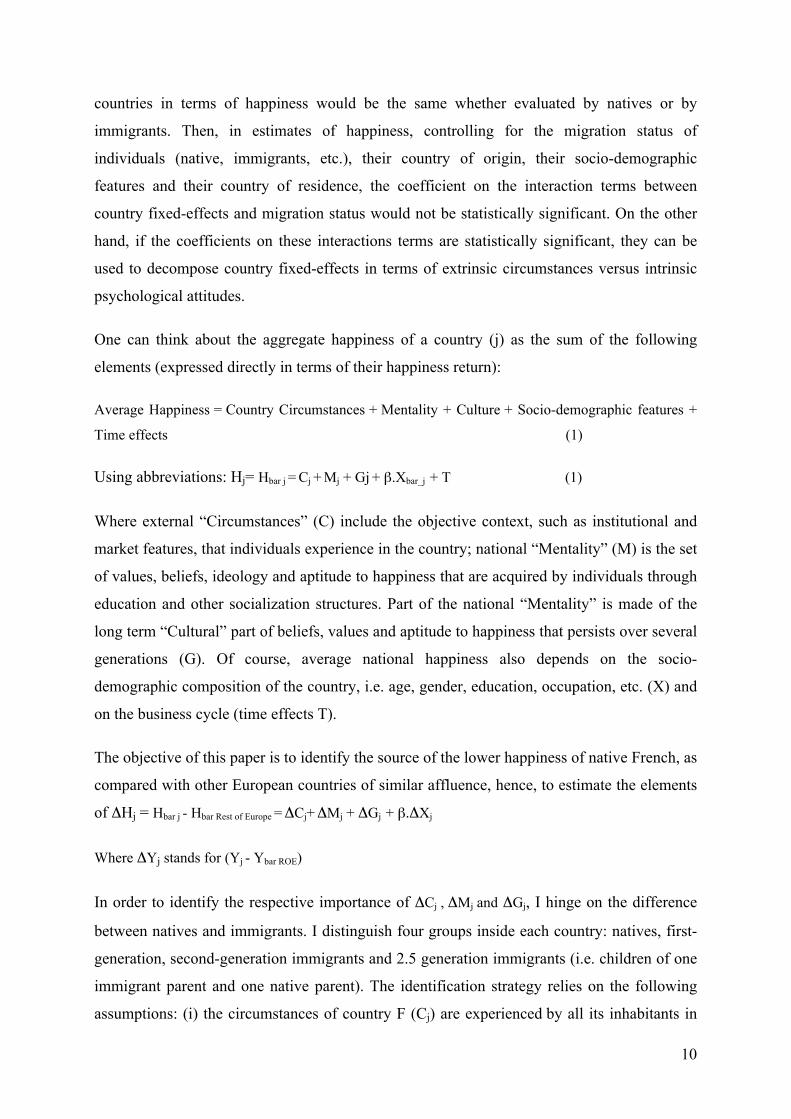
One can think about the aggregate happiness of a country (j) as the sum of the following

elements (expressed directly in terms of their happiness return):

Average Happiness = Country Circumstances + Mentality + Culture + Socio-demographic features +

Time effects (1)

Using abbreviations: Hj= Hbar j = Cj + Mj + Gj + β.Xbar_j + T (1)

Where external “Circumstances” (C) include the objective context, such as institutional and

market features, that individuals experience in the country; national “Mentality” (M) is the set

of values, beliefs, ideology and aptitude to happiness that are acquired by individuals through

education and other socialization structures. Part of the national “Mentality” is made of the

long term “Cultural” part of beliefs, values and aptitude to happiness that persists over several

generations (G). Of course, average national happiness also depends on the socio-

demographic composition of the country, i.e. age, gender, education, occupation, etc. (X) and

on the business cycle (time effects T).

The objective of this paper is to identify the source of the lower happiness of native French, as

compared with other European countries of similar affluence, hence, to estimate the elements

of ΔHj = Hbar j - Hbar Rest of Europe = ΔCj+ ΔMj + ΔGj + β.ΔXj

Where ΔYj stands for (Yj - Ybar ROE)

In order to identify the respective importance of ΔCj , ΔMj and ΔGj, I hinge on the difference

between natives and immigrants. I distinguish four groups inside each country: natives, first-

generation, second-generation immigrants and 2.5 generation immigrants (i.e. children of one

immigrant parent and one native parent). The identification strategy relies on the following

assumptions: (i) the circumstances of country F (Cj) are experienced by all its inhabitants in

11

the same way, independently of their geographical origin; (ii) natives and second-generation

immigrants of country j share the same socialization experience, hence the same Mentality

(Mj), whereas first-generation immigrants have been socialized in a different system; finally,

(iii), immigrants of the first and second-generation still share at least part of the Culture Gk≠F

of their origin country k, while the natives of country F share the Culture of that country (the

GF). Hence, first-generation immigrants are taken to differ from natives by their “Culture” and

“Mentality”; second-generation immigrants only differ from natives by their “Culture”, and

first-generation immigrants differ from second-generation immigrants by their “Mentality”. I

use these difference and double differences (between countries) to identify the share of the

country fixed-effects that can be attributed to Circumstances versus Mentality and Culture.

I treat cultural inertia as a stock that has the same value for immigrants of the first and second

general, and disappears after the second-generation. This cut-point is imposed by the survey,

which, as is generally the rule, report the origin of individuals and of their parents, but not

further. This usual convention probably corresponds to the idea is that cultural differences

take time to dissipate (in the case of the culture of origin) or to acquire (in the case of the

culture of the destination country), and vanishes after two generations. In addition to the

persistent mentality of immigrants, the term G can encompass the specific position of

immigrants in society due to selection effects or discrimination.

The case individuals with one native and one immigrant parent, is less clear-cut. They are

likely to be partly influenced by the culture of origin of their immigrant parent, and to have

received the cultural capital transmitted by their native parent. In order to avoid making any

assumption about the rate of cultural convergence of this generation, I treat them as a separate

category and I do not use them for the identification of ΔCj , ΔMj and ΔGj.

To derive the magnitudes of interest, I estimate a happiness equation on the entire sample of

Europeans, at the individual level (indexed by i). The general form of this equation is the

following:

Hi = α1.I1 + α2.I2 + α3.I3 +∑j µ0j.Dj + ∑j µ1j .I1.Dj + ∑j µ2j.I2.Dj + ∑j µ3j.I3. Dj + β .Xi + ∑k δ k.Ok+ Tt + εi (2)

where I1 is a dummy variable that takes value 1 if the respondent is a first-generation

immigrant (and 0 otherwise), I2 codes for second-generation immigrants, I3 for 2.5 generation

immigrants, Dj is a dummy variable indicating the country of residence of the respondent

(j=1,13) and Ok is a vector indicating the region of origin of the respondent (k=1,6). As shown

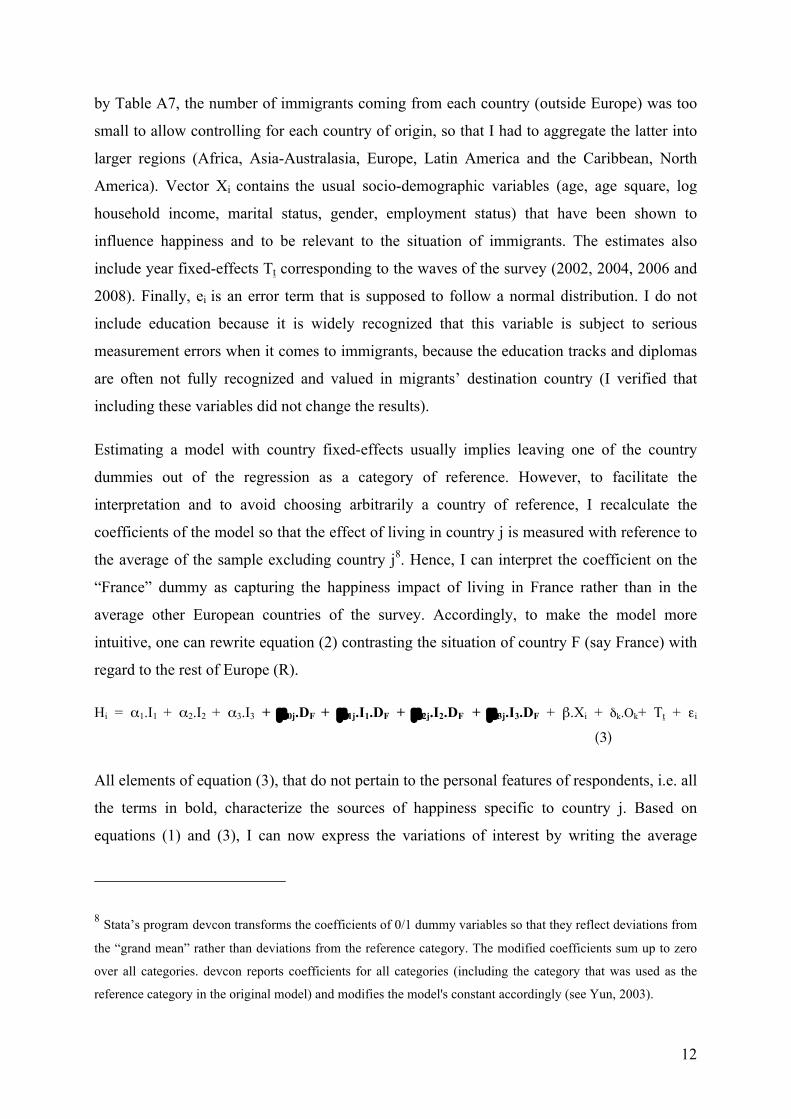
12

by Table A7, the number of immigrants coming from each country (outside Europe) was too

small to allow controlling for each country of origin, so that I had to aggregate the latter into

larger regions (Africa, Asia-Australasia, Europe, Latin America and the Caribbean, North

America). Vector Xi contains the usual socio-demographic variables (age, age square, log

household income, marital status, gender, employment status) that have been shown to

influence happiness and to be relevant to the situation of immigrants. The estimates also

include year fixed-effects Tt corresponding to the waves of the survey (2002, 2004, 2006 and

2008). Finally, ei is an error term that is supposed to follow a normal distribution. I do not

include education because it is widely recognized that this variable is subject to serious

measurement errors when it comes to immigrants, because the education tracks and diplomas

are often not fully recognized and valued in migrants’ destination country (I verified that

including these variables did not change the results).

Estimating a model with country fixed-effects usually implies leaving one of the country

dummies out of the regression as a category of reference. However, to facilitate the

interpretation and to avoid choosing arbitrarily a country of reference, I recalculate the

coefficients of the model so that the effect of living in country j is measured with reference to

the average of the sample excluding country j8. Hence, I can interpret the coefficient on the

“France” dummy as capturing the happiness impact of living in France rather than in the

average other European countries of the survey. Accordingly, to make the model more

intuitive, one can rewrite equation (2) contrasting the situation of country F (say France) with

regard to the rest of Europe (R).

Hi = α1.I1 + α2.I2 + α3.I3 + µ0j.DF + µ1j.I1.DF + µ2j.I2.DF + µ3j.I3.DF + β.Xi + δk.Ok+ Tt + εi

(3)

All elements of equation (3), that do not pertain to the personal features of respondents, i.e. all

the terms in bold, characterize the sources of happiness specific to country j. Based on

equations (1) and (3), I can now express the variations of interest by writing the average

8 Stata’s program devcon transforms the coefficients of 0/1 dummy variables so that they reflect deviations from

the “grand mean” rather than deviations from the reference category. The modified coefficients sum up to zero

over all categories. devcon reports coefficients for all categories (including the category that was used as the

reference category in the original model) and modifies the model's constant accordingly (see Yun, 2003).

13

happiness difference that would be experienced by an individual with the same socio-

economics features (X) and the same origin (Ok) of natives (i.e. controlling for these

variables), depending on his country of residence: F (France) versus the Rest of Europe

(ROE), hence:

• the average happiness difference between first-generation immigrants in country j

versus the Rest of Europe (ROE):

ΔHj1= Hj1 - H ROE 1 = µ0j + µ1j = ΔCj = (Cj – CROE)

• the happiness difference of second-generation immigrants in country j versus the Rest

of Europe (ROE):

ΔΗj2 = Hj2 - HROE 2 = µ0j + µ2j = ΔCj + ΔSj

• the double difference of happiness of natives and second-generation immigrants in

country F versus the rest of Europe:

ΔΗjN − ΔΗj2 = (HN j - HROE j ) - (Hj 2 - HROE 2 ) = - µ2j = ΔGj

• the double difference of happiness between second-generation immigrants and first-

generation immigrants in country j versus the rest of Europe:

ΔΗj2 - ΔΗj1 = µ2j - µ1j = ΔSj

Hence: ΔCj = µ0j + µ1j ΔSj = µ2j - µ1j ΔGj = - µ2j

These parameters are measures of the weight of Circumstances, Mentality and Culture in the

idiosyncratic happiness difference of country j as compared to the rest of Europe. They sum

up to µ0j , which is country j’s fixed-effect measured on natives. I retrieve them using on the

estimation of the happiness equation (2) at the individual level.

Beyond this baseline specification, I also run robustness exercises, allowing for the

interdependence between the different arguments of the happiness function. In particular, I

run Oaxaca-Blinder type simulation and decomposition of the happiness difference between

natives and immigrants living in France, between native French and native Europeans, and

between native French and native Belgians.

14

I then deepen the analysis of the French cultural difference by looking at the happiness of

migrants depending on their schooling experience, the duration of their stay in their

destination country, their country of origin (for Europeans) and their home language.

All the estimates presented in the paper are weighted using the combination of design weight

and population weight that correct for the composition and size of each country’s national

sample (see http://essedunet.nsd.uib.no/cms/userguide/weight/).

IV.  Results  

As a preambule, Table 1 shows that the estimate of equation (2) has the classical properties

uncovered in the happiness literature in terms of age, gender, marital status, income and

employment status (notice the magnitude of this latter variable!). Country fixed-effects are all

statistically significant (as explained, the coefficients have been recalculated in order to

express the effect of living in a particular country as compared with the rest of Europe in

average, i.e. they sum up to zero). As expected, France attracts a negative coefficient, as do

Germany and Portugal; this is also the case of Great-Britain and Slovenia. Living in France

reduces self-declared happiness by 0.23 happiness points (column 1). It reduces the

probability to declare a level of happiness greater than 7 on a 0-10 scale by 19% (column 2).

The lower happiness of the French is attenuated for the young (under 30), the rich (above the

median income) and women, but it is the same for all occupations (estimates not shown for

space reason). Symmetrically, Nordic countries (Denmark, Finland, Sweden, Norway) as well

as Switzerland score high on the ranking. The Danes are 50% more likely to score higher than

7 on the happiness scale! Belgium, Spain and the Netherlands stand in the middle of the

distribution.

1.  Main  results  

The estimation of equation (2) is presented in Table A.1. First and second-generation

immigrants appear to be less happy than natives. This is also the case of individuals with one

immigrant parent, but the coefficient is twice smaller. Immigrants coming from Africa and

Asia are less happy than the average, while those who come form North America are happier

(the other regions are Australasia, Latin America and “unknown”). Column (2) displays the

15

coefficient on country fixed-effects, column (3) the coefficient on the interaction between

country fixed-effects and the fact of being a first-generation immigrant; column (4) the

interaction with second-generation immigrants, and column (5) the interaction with the 2.5

generation (i.e. children of mix immigrant-native couples). As illustrated by Figure 4, which

is based on Table A1, everything else equal, native residents in France, Germany, Great-

Britain, Portugal and Slovenia are less happy than the average Europeans, whereas native

inhabitants of Belgium, the Netherlands, Spain, Switzerland and of course Nordic countries

(Denmark, Sweden, Finland) are happier than the average. But, conditionally on being a first-

generation immigrant, which, as such, implies a lower happiness, those who have chosen

France as a destination country are just as happy as the average immigrant in Europe, whereas

second-generation immigrants seems to converge to the typical level of happiness of natives

(controlling for the region of origin of immigrants).

Table 2 presents the estimates of the different components of the gap between the national

idiosyncratic happiness level of natives and the European average, for each country.

Concerning France, the share of the happiness gap that is due to circumstances (ΔC) is twice

as small as that of Mentality (ΔM) and Culture (ΔG). In several other countries, it is also the

case that the national happiness trait is not associated with the external circumstances of the

country. This is the case of Belgium, Switzerland, Spain and Norway. By contrast, in

Germany and Portugal, the lower level of happiness seems to originate in objective

circumstances to a large extent.

Hence, under the assumptions stated in Section II, the specific unhappiness trait of French

people seems to be due to their values, beliefs and the perception of reality rather than to the

country’s objective general circumstances. Needless to say that this does not mean that

objective circumstances do not explain the level of happiness in France and other European

countries. Rather, the lesson is that the unexplained part of the French unhappiness

specificity, once the effect of measurable objective sources is taken into account, is essentially

of a mental phenomenon.

Additional  Accounting  

The results of Table 2 rely on the assumption that the vector β of coefficients on

circumstances (X) is the same for all groups of the population. In other words, the French

cultural specificity is treated as an additive element that shifts the whole happiness function

16

upwards or downwards. However, this constraint can be relaxed, allowing not only the

constant (shifter) but also the elements of vector β, associated with all the determinants of the

happiness function, to vary across countries and groups of the population. Such simulation

exercises then allow answering questions of the type: how happy would French natives be,

had they the happiness function of migrants? Or the happiness function of Belgians? Or the

happiness function of other European natives?

Accordingly, Table 3.A shows the level of happiness of the population groups of each

country, as predicted by a happiness function (equation 2) estimated on the sample of natives

versus migrants of each country. The actual typical level of happiness of French natives is of

7.215 (column 1), but the predicted level using the parameters obtained on the sub-sample of

immigrants in France is of 7.355 (column 3), hence a difference of 0.14 (column 5). Of

course, the reverse is true, and the typical happiness of immigrants in France (7.246) would

decrease to 7.148 if their exact same circumstances (including the fact of being an immigrants

and their region of origin) were experienced by native French. As illustrated by Table 3.B,

these results are comforted by an Oaxaca (1973) - Blinder (1973) decomposition of the

happiness difference between natives and immigrants in France, which attributes 0.121

happiness points on the account of coefficients, versus -0.087 for endowments, and -0.039 for

interactions between the two (see Jan 2008).

In the same spirit, the upper panel of Table 3.C suggests that whereas the level of happiness

of native French is of 7.222, the average native European, excluding France, would have

reached a level of happiness of 7.539, had he experienced the exact same circumstances as the

native French. Accordingly a decomposition à la Oaxaca-Blinder suggests that endowments

explain only 0.166 points of the difference between native French and other European natives,

whereas coefficients explain 0.285 (Table 3.D).

Finally, to be more concrete, one can compare France and Belgium, two close neighboring

countries sharing a common language. As shown by the lower panel of Table 3.C, if the

French circumstances were experienced by native Belgians instead of native French, the

average happiness of natives would be of 7.64 instead of 7.22. And if the French natives lived

in Belgium (but kept their mentality), their average happiness level would only be of 7.39

instead of the level of 7.74 experienced by Belgians. Table 3.E confirms that the average

happiness difference between the two countries (0.52) is much better explained by

coefficients (0.411) than by endowments (0.207).

17

These differences are equivalent to a variation by about 2% in average income (which is

approximately the annual growth rate of national income in these countries over the

considered period). One may think that the order of magnitude of these figures is not very

impressive. This is due to the narrow range of variation of self-declared happiness, which

overall mean value in the ESS is of 7.61 with a standard deviation of 1.69. Hence, the

mentioned variations represent about one sixth of the standard deviation of the happiness

variable. Moreover, as shown by the tables of this paper, in a typical happiness regression, the

share of happiness that is explained by observable variables is small; the typical R2 of an OLS

estimate of happiness varies between 3% and 15% depending on the controls that are

included. The small range of variation of happiness is a general fact that is well-known by the

specialists of the field (See Clark and Senik 2011 for a discussion of this point).

2.  Channels  of  Mentality  and  Culture  

Tables 4 to 7 explore the channels of formation and transmission of Mentality and Culture in

the French case. They look at the effect of schooling in France on immigrants’ happiness, as

well as the effect of their duration of stay. They also look at the relative level of happiness of

the French living in foreign countries. Finally, I follow the analysis of cultural transmission

by Luttmer and Singhal (2011) and estimate the correlation between the happiness of

migrants and the typical happiness of their compatriots in their home country.

Schooling  in  France  

The effect of schooling in France has already been captured, in the main specification (Table

A1 and Figure 4), which showed that first-generation immigrants in France (whose majority

has not been in school in France) are happier than second-generation immigrants (who have),

and are also happier than the average first-generation immigrants in other European countries;

whereas second-generation immigrants to France are less happy than the average second-

generation immigrants to other European countries. This section tries to be more specific.

The ESS survey does not include direct information about whether respondents have been to

school in their country of residence or not. However, it includes a variable that indicates how

long ago the respondent first came to live in the country. The modalities of the answer are

“within last year” (2%), “1-5 years ago” (17.7%), “6-10 years ago” (14.4%), “11-20 years

ago” (23.8%) and “more than 20 years ago” (44.1%). Using the age of the respondent and his

answer to the latter question, I construct a variable indicating whether immigrant respondents

18

have attended school in their destination country at least since the age of 10. Admittedly, with

this method, I cannot guess whether respondents older than 31 years were in school in their

destination country at the age of 10. Accordingly, I also run the estimates on the sub-sample

of immigrants aged 18 to 31 years old.

As shown by Table 4, first-generation immigrants who went to school in France before the

age of 10 are less happy than those who did not (columns 3 and 4 of the table). Column (3)

treats all immigrants over 32 years old as not having attended school in France, which is

certainly incorrect: hence, it underestimates the effect of schooling on happiness attitudes.

This is confirmed by the results presented in column (4), where the sample is restricted to

first-generation immigrants under the age of 33: the coefficient on the variable of interest is

twice as large as in the specification of column 1. Concerning the main effects, the coefficient

on the France fixed effect is either not significant or positive, consistently with the previous

result that immigrants do not share the specific French unhappiness. Notice that schooling in

Germany and Portugal does not seem to exert the same depressing effect (the opposite is

true), consistently with the previous finding that the lower happiness of the German is due to

objective circumstances as much as to mentality or culture.

Staying  in  France  

Table 5 estimates the happiness of first-generation immigrants depending on their duration of

stay in their destination country. The data is well fitted by a quadratic function of the duration

of stay. I interact the first two terms of a second-degree polynomial function of the duration of

stay with immigrants’ country of destination. The interaction terms for France predict an

increase in the happiness of migrants to France followed by a reversal approximately 20 years

after their arrival.

The  French  Abroad  

If it I true that happiness has a persistent cultural dimension, it should be the case that the

French (for instance) are less happy than other Europeans in average even when they live in a

foreign country. Table 6 shows that among migrants of either generation having moved from

one European country of the sample to another one, the French are statistically significantly

less happy than the average, whether the estimates control for the country of residence (as in

column 1) or not (column 2). A French origin reduces the level of declared happiness by

about 0.11 as compared to the average European origin.

19

Most coefficients on the country of origin of European migrants are statistically significant,

which suggests that the psychological and cultural dimensions of happiness are important in a

general way. To comfort this observation, I replicated the exercise of Luttmer and Singhal

(2011) and tested whether the happiness of European migrants is correlated with the average

happiness in their origin country. Table 7 presents estimates of happiness run over the sample

of European migrants (first and second generations); it shows that the coefficient on the

average happiness calculated over natives in the origin country of migrants is positive and

statistically significant. In the same line, the estimates presented in columns (3) and (4)

include the coefficient of happiness on country fixed-effects, estimated in a first stage

regression on the sample of natives, controlling for the usual socio-demographic variables.

Both specifications lead to the same “epidemiological” results, that the happiness of migrants

depends on the typical happiness level of people living in their home country. This can be

interpreted, in the spirit of Luttmer and Singhal, as testifying to the cultural dimension of

happiness.

3.  Language:  culture  or  scaling  

Country fixed-effects could also be due to language and translation effects, if happiness

statements depend on the language in which they are expressed, or if different nations

associate a different verbal label to a given internal feeling. Country fixed-effects would then

boil down to purely nominal scaling effects (see section Section I). To address this issue, I

look at the typical happiness of different linguistic groups inside three multilingual countries.

If the French unhappiness is purely nominal, we should observe that in a given country,

francophone regions and individuals are less happy than non-francophone ones.

Using the ESS, I look at the case of Belgium and Switzerland (10 000 observations). In

Belgium, three regions are distinguished: Wallonia, Flanders and Brussels. Table 8.A shows

that controlling for the usual socio-economic circumstances (age, gender, income,

unemployment, marital status), as well as for year dummies (which account for the business

cycle), living in a Walloon region reduces the typical individual level of happiness by 0.22

happiness points. Controlling for the regions where they live (column 2) or not (column 3),

francophone individuals are less happy than Dutch-speaking ones (by 0.26 happiness points).

However, in Switzerland it is not the case that French-speaking individuals are less happy

than German-speaking ones. Table 8.B shows that it is the Italian-speakers (columns 1 and 3)

and the Italian-speaking regions (column 2) that are statistically significantly less happy, as

20

compared to German-speakers. Controlling for the regional language (columns 2 and 3) or not

(column 1), native Francophones appear to be just as happy as German-speakers.

I also used the Canadian sample of the World Values Survey available for years 2000 and

2006 (3461 observations, see descriptive statistics in Table A10). The data include

information about the language in which the interview was realized, and the language that

people declare they use predominantly at home. In this survey, 68% of respondents declared

that English is their home language, 26% French and 5% another language. Table 8.C shows

that francophone individuals are happier than English-speaking ones (by about 5%),

controlling for a series of objective circumstances, such as the usual socio-demographic

features, year fixed-effects and the self-declared ethnic group of respondents.

I take these observations as a sign that the difference in the level of happiness of the French is

cultural9, but not purely nominal.

4.  Emotional  well-­‐being  

In the same line, it is useful to check whether alternative measures of well-being focusing on

emotions and affects lead to a similar picture of the French in the hierarchy of European

nations. These measures capture “short run utility” (Kahneman, 1999), as opposed to the more

cognitive and judgmental “long-run utility” that is measured by life satisfaction or happiness

questions (see Diener et al. 2010, or Kahneman et al. 2010). Such reported affects are often

collected using the Experience Sampling Method or the Day-Reconstruction-Method, or time-

use surveys, where respondents have to qualify the emotions they experience during each of

their daily activities (see Diener et al. 2010, or Kahneman et al. 2010). This method was

followed by the Gallup World Poll, which conducted surveys of representative samples of

people from 155 countries between 2005 and 2009, asking individuals to report the emotions

they experienced during the previous day. Questions were worded as follows: “Did you

9 Brügger, Lalive and Zweimuller (2008) have advocated the importance of cultural differences, as vehicled or

expressed by linguistic barriers. They show that preference for leisure differs on either parts of the linguistic

barrier in Switzerland (the Barrière des Roesties or Röstigraben) that separates German-speaking regions from

regions speaking languages derived from Latin (French, Romansh and Italian). They argue forcefully that the

observed differences are due to cultural inertia rather than objective circumstances of the regional labor markets.

21

experience the following feelings during a lot of the day yesterday? How about _____?” Each

of several emotions (e.g., enjoyment, smile (Did you smile a lot yesterday?), happiness,

worry, sadness, anger, stress) was reported separately, using had yes/no response options. I

used the country mean frequency of reported affects for the same European countries as

analyzed in the rest of the paper10 (when available in the Gallup World Poll), for years going

from 2007 to 2009. Following the usage, I built an average positive affect score and an

average negative affect score, as well as an average net score of positive minus negative

answers.

As shown by the Figures 5.A to 5.C, it turns out that France ranks first in terms of negative

affects! This is due to the particularly high number of French respondents reporting feelings

of anger (see the descriptive statistics in Table A11). The ranking of countries in terms of net

affects balance (positive affects minus negative affects) is similar to the one obtained with

Life Satisfaction, with Slovenia in the lowest place, near Spain, Portugal and France, and

Nordic countries at the top. Hence, measures of emotional well-being lead to the same picture

of international differences as measures of Life Satisfaction.

5.  Beyond  Happiness  

If, conformingly with the findings of section III.1, the lower happiness of the French is not

due to circumstances but to the way they perceive them, this should also appear in the other

attitudes and values that they endorse. Table 9.A presents estimates of a series of satisfaction

attitudes, while Table 9.B deals with more diverse opinions.

Table 9.A includes an estimate of a depressiveness score (column 1), built with questions of

the third wave of the ESS (hence the smaller number of observations) that were inspired by

the well-known CES-depression scale D (Radloff 1977). These questions asked the

respondent how often, during the past week, he “felt depressed”, “felt everything he did was

effort”, “sleep was restless”, “felt lonely” “felt sad, “could not get going”, “felt anxious”, “felt

tired” “felt bored”, “felt rested when woke up in morning, “seldom time to do things he really

enjoy”, “feel accomplishment from what he did”, “in general feel very positive about

10 I am grateful to Angus Deaton for obtaining the authorization for me to use these data.

22

oneself”, “always optimistic about one’s future”, “at times feel as if he is a failure”, choosing

an answer on a scale going from 1 “none or almost none of the time”, 2 “some of the time”, 3

“most of the time”, 4 “all or almost all of the time”. (I recoded the scales in order to obtain a

score that increases with depression symptoms). By summing up the number of points on

these different questions, I obtain an index of depressiveness that runs potentially from 5 to

59. In the regression sample, it takes values from 5 to 57, with an average value of about 20.

France has a score of 22, in the vicinity of Portugal and Great-Britain.

Tables 9.A and 9.B offer several lessons. French natives are more depressive and less

satisfied on all the dimensions measured by the survey, except satisfaction with the health

system (see also Deaton, 2008, Figure 5 p.68, for a similar finding). They are less satisfied

with the state of the economy in the country, with the state of democracy, with the state of the

education system. Probit estimates (not shown) show that living in France reduces the

probability to be very satisfied with these dimensions (over 7 on a 0-10 scale) by 12% to 20%.

It increases the probability of declaring that one lives difficultly with one’s household’s

income by 24% (controlling for household income). It also reduces the probability to declare

that “most people can be trusted” or that “most people try to be fair”. Second, concerning

more general opinions, native French are less confident in the possibility of finding a similar

or better job with another employer, or in the easiness of starting one’s own business. They

agree more often that it is important that people are have equal opportunities, that the state

should reduce the income difference between the poor and the rich, that differences in the

standard of living should be kept small and that it is important that the government is strong;

they more often disagree with the idea that large income differences are acceptable to reward

talents and efforts. Hence, the specific unhappiness of the French is mirrored by their general

attitudes, beliefs and values.

5.  Robustness  

The essential element of the identification strategy is the differential happiness effect of

common circumstances across different population groups (natives, migrants). I thus need to

be sure to compare the comparable.

First, the specific happiness trait of the French could be due to some macroeconomic

circumstances that are poorly measured at the individual level. I thus included successively in

the estimates of happiness (equation 2) the growth rate of GDP, unemployment rate, inflation

23

rate, yearly GDP per capita, number of worked hours per week, life expectancy at birth, as

well as the weight of government expenditure over GDP (taken from the World Bank’s World

Development Indicators). As shown by Table A2 in the Appendix, none of these magnitudes

turned out to be statistically significant, except inflation (negative coefficient). Including them

did not change the magnitude or sign of the coefficients on country dummies and interactions

between country dummies and categories of origin (first and second-generation). It also did

not change the order of magnitude of the parameters of circumstances, mentality and culture

(displayed at the bottom of the table).

Beyond this basic verification, one needs to address the potential unobserved heterogeneity in

the sources of well-being of migrants versus natives. The specification of equations (1) - (3)

relies on the general simplifying assumption that the effects of socio-demographic features,

country circumstances, migration status and region of origin are separable (in an additive

way). Of course, these are strong assumptions. The main problem would be if migrants to

different countries had different characteristics that, themselves, had different effects on

happiness across countries, especially if migrants self-selected to different countries

depending on these differences. In this case, the difference in the country fixed-effects

measured on native versus immigrants would be causal and due to some common

macroeconomic factor (the size of budget transfers for instance).

In the absence of the ideal dataset (that would ensue from a randomized allocation of

immigrants to European countries), I can only try to overcome these problems by controlling

for the potential sources of heterogeneity that are observable. I run several robustness tests

that consist in including triple interaction terms between magnitudes that are suspected of

being interdependent (together with main effects and simple interactions). The equations to

estimate are of the type:

Hi = α1.I + β.Xi + δ.Ok + φ.Zi + µ0j.Dj + γ2j.I.Dj + γ3.I.Zi + γ4j.Dj.Zi + γ5j.I.Dj.Zi + Tt + Tt* Zj + εi (4)

where Zi is the potential source of heterogeneity, I stands for the fact of being an immigrant

(versus native11), Dj is the destination countries. Hence, γ3 will measure the specific effect of

11 Because of the small number of observations, I simply distinguish natives from immigrants (pooling together

the first and second generations).

24

being an immigrant and having feature Z; while γ5j measures the effect of variable Z on

immigrants to France rather than to other destination countries, as compared with French

natives. For simplicity, equation (4) contrast country j (say France) to the rest to Europe. Year

fixed-effects were included in the estimates, as well as their interaction with the aggregate

controls Tt* Zi (this is to control for the potential country specific time trend in these

magnitudes).

If the coefficient γ5j on the triple interaction term is not statistically significant, one cannot

reject the fundamental hypothesis that indeed, the magnitudes are separable. Table A3 and A4

present the results of the estimates of equation (4). For space concerns, they only display the

coefficients on the variables of interest and their simple and double interactions with the

France dummy variable.

Macroeconomic  channels  

It turns out (Table A3) that none of the triple interactions between macroeconomic controls,

migration status and France fixed-effect is statistically significant. This implies that one

cannot reject the null that country fixed-effects and differences between natives and

immigrants are not driven by some country macroeconomic specificity (such as transfers,

budget spending, or unemployment benefits). Note that happiness declines less with aggregate

unemployment in France than it does in average in Europe.

Individual  channels  

I consider the following sources of individual heterogeneity (Z): gender, income (“Rich”: a

dummy for above-average income), age (a dummy “Young” indicating whether the

respondent was less than 30 years old, which is the case of 26% if immigrants), being

unemployed, receiving state transfers, occupation (ISCO, 1 digit level) and region of origin.

Table A4 shows that, although the coefficients on simple interactions were often statistically

significant, those on the triple interaction term (γ5j) were not, except for employment status:

unemployed migrants to France were relatively happier than in the rest of Europe (see Clark

2003 for a discussion of unemployment as a social norm). However, migrants to France who

received State transfers were relatively less happy than in the rest of Europe (although the

coefficient is not well determined). The coefficients on triple interaction terms between

country fixed-effects, migration status and occupation categories (as measured by ISCO-1

25

digit) were not significant. The same is true of triple interactions between country fixed-

effects, migration status and regions of origin.

Overall, robustness test do not allow rejecting the null hypothesis of separability between the

factors on which the identification strategy of the components of the French specific

unhappiness relies.

Conclusions  

This paper has devoted a special attention to France, which appears as an outlier in

international studies of happiness. However, beyond the case of France, it underlines the

important cultural dimension of happiness. The lesson is relevant for policy-makers who have

recently endeavored to maximize national well-being and not only income per capita.

“Happiness policies” should take into account the irreducible influence of psychological and

cultural factors. As those are -at least partly- acquired in school and other early socialization

instances, this points to some new aspects of public policy such as considering the qualitative

aspects of the education system.

Investigating the causes of the differences in the cultural dimension of happiness across

countries is beyond the objectives of this paper, but certainly constitutes an interesting avenue

for future research. The economics of culture could help understanding the how culturally

determined idiosyncratic happiness originates in national institutions and history. The cultural

dimension of happiness is also undoubtedly the opportunity for a fruitful encounter between

economics and psychology.

26

References  

Alesina A. and Fuchs-Schündeln N. (2007). “Good Bye Lenin (or Not?): The Effect of Communism on People’s Preferences,” American Economic Review, 97(4): 1507-28.

Alesina, A. and Giuliano P. (2007). “The Power of the Family,” NBER WP n°13051.

Alesina, A. and Giuliano P. (2011). “Preferences for Redistribution,” in Benhabib J., Bisin A. and O’Jackson M. (eds.) Handbook of Social Economics, 93-132.

Algan Y. and Cahuc P. (2010). “Inherited Trust and Growth”, American Economic Review, 100, 2060–2092.

Algan Y. et Cahuc P. (2007). La société de défiance : comment le modèle social français s'autodétruit ? Paris : Ed. ENS rue d'Ulm, 102 p. Opuscule n°9 - ISBN 978-7288-0396-5.

Algan Y., Aghion P and Cahuc P. “The State and the Civil Society in the Making of Social Capital”, Journal of the European Economic Association, forthcoming.

Algan Y., Aghion P., Cahuc P. and Shleifer A. (2010). “Regulation and Distrust”. Quarterly Journal of Economics, 2010.

Altonj J., Blank R. (1999) “Race and gender in the Labor Market”. Chapter 48, Handbook of Labor Economics, volume 3.

Amit, K. (2010), “Determinants of life satisfaction among immigrants from Western countries and from the FSU in Israel”. Social Indicators Research, forthcoming

Baltatescu, S. (2007). “Central and Eastern Europeans migrants ‘subjective quality of life: a comparative study”. Journal of identity and migration studies, 1(2), 67-81

Bartram D. (2011) “Economic Migration and Happiness: Comparing Immigrants' and Natives' Happiness Gains from Income”, Social Indicators Research.

Beegle K., Himelein K. and Ravallion M. (2009). “Frame-of-reference bias in subjective welfare regressions”. World Bank Policy Research Working Paper 4904.

Bisin A. and Verdier T. (2001). “The Economics of Cultural Transmission and the Dynamics of Preferences”. Journal of Economic Theory 97:298-319.

Bisin A. and Verdier T. (2011). “The economics of cultural transmission and socialization”, in Benhabib J., Bisin A. and O’Jackson M. eds. Handbook of Social Economics, 339-416.

Bisin A., G. Topa and Verdier T. (2004). “Religious Intermarriage and Socialization in the US”, Journal of Political Economy, 112, 615-665.

Blinder A. (1973). “Wage Discrimination: reduced Form and Structural Estimates”. The Journal of Human Resources 8: 436:455.

27

Borjas G. (1992). “Ethnic Capital and Intergenerational Mobility”. Quarterly Journal of Economics: 123-150.

Borjas G. (1995). “Ethnicity, Neighborhoods, and Human-Capital Externalities”. American Economic Review 85: 365-390.

Brulé G., Veenhoven R. (2012). “Why are Latin Europeans less happy? The impact of social hierarchy”, forthcoming in Anthropology. ISBN 979-953-307-388-9

Briot M. (2006). Office parlementaire d’évaluation des politques de santé. Sur le bon usage des medicaments psychotropes. http://www.assemblee-nationale.fr/12/pdf/rap-off/i3187.pdf

Brügger B., Lallive R. and Zweimüller J. (2008). “Does Culture Affect Unemployment? Evidence from the Barrière des Roestis”, mimeo.

Clark A. (2003). “Unemployment as a Social Norm: Psychological Evidence from Panel Data”, Journal of Labor Economics, 21, 323-351.

Clark A. and Senik C. (2011). “Will GDP Growth Increase Happiness in Developing Countries?”, PSE WP n°2010-43 and Proceedings of the AFD-EUDN conference (Paris, December 2010), forthcoming.

Clark, A., Frijters, P., and Shields, M. (2008). "Relative Income, Happiness and Utility: An Explanation for the Easterlin Paradox and Other Puzzles". Journal of Economic Literature, 46, 95-144.

Commmission of the European Communities (2009). GDP and Beyond. Measuring progress in a Changing World. Communication from the Commission to the Council and the Euopean Parliament.

Cronbach L. (1946). “Response set and test validity”. Educational and Psychological Measurement, 6, 475-794.

Crowne D. and Marlowe D. (1960). “A new scale of social desirability independent of psychopathology”. Journal of Consulting Psychology, 24(4), 349-354.

d’Iribarne P. (1989). La logique de l’honneur, Seuil.

De Jong, G.F., Chamratrithirong, A., Tran, Q.-G (2002). “For better, for worse: life satisfaction consequences of migration”. International Migration Review, 36(3), 838-63

Deaton A. (2008). “Income, Health, and Well-Being around the World: Evidence from the Gallup World Poll”. Journal of Economic Perspectives, 22(2), 53–72.

Di Tella, R. et MacCulloch R. (2006). “Some Uses of Happiness Data in Economics”, Journal of Economic Perspectives, 20, 25-46.

Di Tella, R., MacCulloch, R.J., and Oswald, A.J. (2003). "The Macroeconomics of Happiness". Review of Economics and Statistics, 85, 809-827.

Diener E., Helliwell J. and Kahneman D. (2010). International Differences in Well-Being. Oxford University Press.

28

Diener E., Kahneman D., Tov W. and Arora R. (2010). “Income’s association with Judgements of Life versus Feelings”, Chapter 1 (pp 3-16) in Diener E., Helliwell J. and Kahneman D. eds. International Differences in Well-Being. Oxford University Press.

Kahneman E., Schkade D., Fischler D., Krueger A. and Krilla A. (2010.) “The Structure of Well-Being in Two Cities: Life Satisfaction and Experienced Happiness in Columbus , Ohio, and Rennes, France”, Chapter 2 (pp 16-34) in Diener E., Helliwell J. and Kahneman D. eds. International Differences in Well-Being. Oxford University Press.

Diener, E., Suh, E. M. (Eds.). (2000). Culture and Subjective Well-Being Cambridge, MA: MIT Press.

EC (2004). The State of Mental Health in the European Union, European Communities, ISBN 92-894-8320-2.

Edwards A. (1990). “Construct validity and social desirability”. American Psychologist, 45, 287-289.

Eugloreh (2007). Global Report on the Status of Health in the European Union. http://www.eugloreh.it/ActionPagina_979.do

Eurostat (2010). Feasibility study for Well-Being Indicators.

Eysenck H and Eysenck S. (1975). Manual of the Eysenck Personality Questionnaire. London: Holder and Stoughton.

Fernández R. (2007). “Women, Work, and Culture,” Journal of the European Economic Association, 5(2-3): 305-332.

Fernández R. (2008). “Culture and Economics,” New Palgrave Dictionary of Economics, 2nd edition, Stephen Durlauf and Lawrence Blume (eds.), New York: Palgrave Macmillian.

Fernandez R. (2011). “Does Culture Matter?”, in Benhabib J., Bisin A. and O’Jackson M. eds. Handbook of Social Economics, 481-510.

Fernandez R. and Fogli A. (2006). “Fertility: The Role of Culture and Family Experience”, in Journal of the European Economic Association.

Fernandez R. and Fogli A. (2009). “Culture: An Empirical Investigation of Beliefs, Work, and Fertility”, American Economic Journal: Macroeconomics.

Ferrer-i-Carbonell, A. and P. Frijters (2004). “How important is methodology for the estimates of the determinants of happiness?” The Economic Journal, 114: 641-659.

Frey, B.S. and A. Stutzer (2002), “What can Economists Learn from Happiness Research?”, Journal of Economic Literature, 40, 402-435.

Guiso L., Sapienza P. and Zingales L. (2006). “Does Culture Affect Economic Outcomes?”, Journal of Economic Perspectives, 20(2): 23-48.

29

Heston A., Summers R. et Aten B., 2009. Penn World Table Version 6.3. Center for International Comparisons of Production, Income and Prices at the University of Pennsylvania.

Hopkins D. and King G. (2010). “Improving anchoring vignettes: designing surveys to correct interpersonal incomparability”, mimeo, Harvard University.

Huppert H., Marks N., Clark A.E., Siegrist J., Stutzer A., Vittersø J. and Wahrdorf M. (2009). "Measuring well-being across Europe: Description of the ESS Well-being Module and preliminary findings". Social Indicators Research, 91, 301-315.

Inglehart, R., Foa, R., Peterson, C., and Welzel, C. (2008). "Development, Freedom, and Rising Happiness: A Global Perspective (1981–2007)". Perspectives on Psychological Science, 3, 264-285.

Jagger C ., Gillies C., Moscone F., Cambois E., Van Oyen H., Nusselder W., Robine J-M., and the EHLEIS team, (2008). “Inequalities in healthy life years in the 25 countries of the European Union in 2005: a cross-national meta-regression analysis”. Lancet, 372: 2124–31.

Jann. B. (2008). “The Blinder–Oaxaca decomposition for linear regression models”, Stata Journal 8(4).

Kahneman, D. and A.B. Krueger (2006). “Developments in the Measurement of Subjective Well-being”, Journal of Economic Perspectives, 22, 3-24.

Kapteyn A., Smith J. and Van Soest A. (2007). “Vignettes and self-reported work disability in the US and the Netherlands”. American Economic Review, 87(1), 461-473.

Kapteyn A., Smith J. and Van Soest A. (2008). “Comparing Life Satisfaction”. Working Paper WR-623, Rand Corporation.

King G., Murray C., Salomon J. and Tandon A. (2003). “Enhancing the validity and cross-cultural comparability of measurement in survey research”. The American Political Science Review, 97(4), 567-583.

Layard, R. (2005). Happiness: Lessons from a new science. London: Penguin.

Luttmer E. and Singhal M. (2011). “Culture, Context, and the Taste for Redistribution”, American Economic Journal: Economic Policy, 3(1):157-79.

McCrae R and Costa P. (1983). “Social desirability scales: more substance than style”. Journal of Consulting and Clinical Psychology, 51, 1349-1364.

Paulhus D. (1984). “Two-Component Models of Socially Desirable Responding”. Journal of Personality and Social Psychology, 46(2), 598-609.

Paulhus D. (1991). “Measurement and control of response bias”. In Robinson, Shaver and Wrightsman(eds.) Measures of personality and social psychological attitudes. New York: Academic Press, 17-59.

Paulhus D. (1994). Balanced Inventory of desirable responding. Reference manual for BIDR version 6. Vancouver: University of British Columbia, Mimeo.

30

OECD (2011), How's Life?: Measuring well-being, OECD Publishing. http://dx.doi.org/10.1787/9789264121164-en OECD (2009). “Comparative Child Well-Being across the OECD”, chapter 2 in Doing Better for Children, ISBN 978-92-64-05933-7. Portes, A. and M. Zhou (1993), “The New Second Generation: Segmented Assimilation and Its Variants”. Annals of the American Academy of Political and Social Science 530:74-96.

PWT 7.0 Alan Heston, Robert Summers and Bettina Aten, Penn World Table Version 7.0, Center for International Comparisons of Production, Income and Prices at the University of Pennsylvania. (2011).

Radloff, L. S. (1977). “The CES-D scale: A self-report depression scale for research in the general population”. Applied Psychological Measurement, 1, 385–401.

Safi, M. (2010). “Immigrants' life satisfaction in Europe: between assimilation and discrimination”. European Sociological Review vol. 26(2), 159-176

Saint-Paul G. (2010). “Endogenous Indoctrination: Occupational Choice, the Evolution of Beliefs, and the Political Economy of Reform”, The Economic Journal, 120 (544), 325-353.

Saris W. (1998). “The effect of measurement error in cross-cultural research”. ZUMA Nachrichten Spezial, 67-83.

Stiglitz J., Sen A. and Fitoussi J-P (2009). Report by the Commission on the Measurement of Economic Performance and Social Progress. OECD.

Van de Vijver F. (1998). “Towards a theory of bias and equivalence”. ZUMA Nachrichten Spezial, 1-40.

Van Soest A., Delaney L., Harmon C., Kapteyn A. and Smith J. (2007). “Validating the use of vignettes for subjective threshold scales”. Geary WP/14/2007.

Waldron S. (2010). “Measuring Subjective WellBeing in the UK”, Office for National Statistics Working Paper.

Wolfers, J. and B. Stevenson (2008), “Economic Growth and Subjective Well-Being: Reassessing the Easterlin Paradox”, Brookings Papers on Economic Activity, Spring.

Yun, M.-S. (2003). “A Simple Solution to the Identification Problem in Detailed Wage Decompositions”. IZA Discussion Paper No. 836.

ZUMA (1998). Nachrichten Special (special issue dedicated to cross-cultural research and equivalence problems).

  30  

Tables    

Figure  1.A    GDP  and  Average  National  Happiness  (0-­‐10  scale)      

Source: ESS (waves 1- 4) Figure  1.B    Human  Development  Index  and  Average  National  Happiness  (0-­‐10  scale)      

 Source: ESS (waves 1- 4)

  31  

Figure  2.  Happiness,  Income  …  and  Cultural  Factors  around  the  World  

Source : Inglehart, Foa, Peterson, Welzel (2008), p. 269

 Figure  3.A  Average  Life  Satisfaction  over  time  (0-­‐4  scale)  

Source: Eurobarometer

  32  

Figure  3.B  Average  Satisfaction  (0-­‐4  scale)  and  GDP  per  Capita    

Source: Eurobarometer and WDI

  33  

Table  1.  Basic  Estimates  of  Happiness  

OLS

Happy (0-10 scale)

Probit Estimates. Probability that Happiness>7

Marginal effects displayed Age -0.0706*** -0.041*** (0.00805) (0.005) Age square 0.0695*** 0.038*** (0.0102) (0.005) Male -0.143*** -0.117*** (0.0279) (0.024) Log (Household income) 0.366*** 0.239*** (0.0410) (0.021) Married 0.456*** 0.324*** (0.0392) (0.045) Divorced -0.117** -0.077*

(0.0470) (0.040) Widowed -0.454*** -0.179** (0.0823) (0.071) Unemployed -0.626*** -0.345*** (0.0925) (0.040) Belgium 0.0706*** 0.041*** (0.00449) (0.004) Switzerland 0.180*** 0.167*** (0.0242) (0.012) Germany -0.429*** -0.230*** (0.00540) (0.001) Denmark 0.574*** 0.495*** (0.0151) (0.006) Spain 0.0755*** -0.048*** (0.0150) (0.010) Finland 0.422*** 0.400*** (0.00262) (0.002) France -0.231*** -0.191*** (0.00945) (0.011) Great-Britain -0.282*** -0.196*** (0.00594) (0.004) Netherlands 0.0922*** 0.079*** (0.00439) (0.003) Norway 0.102*** 0.056*** (0.0240) (0.012) Portugal -0.589*** -0.606*** (0.0341) (0.017) Sweden 0.202*** 0.158*** (0.00922) (0.007) Slovenia -0.186*** -0.126*** (0.0267) (0.015) Constant 6.330*** -0.600*** (0.274) (0.172)

  34  

R-squared 0.130 0.076 Observations 65378 65461 Observed P at x-bar 0.633 Predicted P at x-bar 0.642 Log Likelihood -39758

Other controls: year fixed-effects. Robust standard errors clustered by country. Weighted estimates. Reference categories: single, in paid work. The coefficients of country fixed-effects reflect deviations from the “grand mean” rather than deviations from the reference category. The modified coefficients sum up to zero over all categories.  

  35  

Figure  4.  Total  Country  Fixed-­‐Effects  by  Migration  Status  Based  on  Probit  Estimates.    

Marginal  Effects  Displayed.  Probability  to  declare  a  level  of  happiness  over  7  on  a  0-­‐10  scale.  

 

 

 

 

 

 

 

 

 

 

 

 

 

 

 

Source: ESS (waves 1- 4)  

Table  2.  Derivation  of  Parameters  Based  on  the  Estimation  of  Equation  (2)  

Decomposition  of  the  Gap  in  Idiosyncratic  National  Happiness  that  is  due  to  Circumstances,  Mentality  and  Culture  

(1) (2) (3) (4)

Circumstances

(µ0j + µ1j) Mentality

(µ2j − µ1j) Culture

(-µ2j) Natives fixed-effect (µ0j ) (sum of columns 1 + 2 + 3)

Belgium 0.01 -0.22 0.29 0.08 Switzerland 0.02 -0.10 0.33 0.24 Germany -0.36 -0.18 0.22 -0.33 Denmark 0.65 -0.25 0.18 0.58 Spain 0.08 0.51 -0.52 0.08 Finland 0.34 0.52 -0.46 0.40 France -0.05 -0.10 -0.11 -0.26 G-B -0.20 -0.55 0.51 -0.24 Netherlands 0.21 -0.16 0.02 0.07 Norway 0.03 -0.02 0.10 0.12 Portugal -0.52 -0.06 -0.09 -0.68 Sweden 0.12 0.02 0.09 0.22 Slovenia -0.30 0.59 -0.56 -0.26

Note: These are measures of the gap between national happiness and the European average that is due to each factor. Consequently, all columns sum to zero. For example, the happiness gap between French natives and European natives is of -0.26, of which -0.05 is attributable to objective circumstances, -0.10 to Mentality and -0.11 to Culture. Coefficients derived from the estimate of equation (2) presented in Table A1 (see Section III for formulae).

-0,8 -0,7 -0,6 -0,5 -0,4 -0,3 -0,2 -0,1

0 0,1 0,2 0,3 0,4 0,5 0,6 0,7 0,8 0,9

PT DE FR SI GB NL BE ES NO SE CH FI DK

Natives

1st generation

2nd generation

  36  

Table  3.A    Simulating  the  Happiness  of  Natives  with  the  Parameters  of  Immigrants  and  vice-­‐versa  

happy

(1) Actual

Happiness of Natives

(2) Actual

Happiness of Immigrants

(3) Happiness of Natives with Parameters of Immigrants

(4) Happiness of Immigrants

with Parameters of

Natives

(5) Happiness

Gap of Natives due

to Parameters (1-3)

(6) Happiness Gap of Immigrants

due to Parameters (2-4)

Belgium 7.744 7.488 7.663 7.679 0.081 -0.190 Switzerland 8.058 7.823 7.879 8.062 0.179 -0.240 Germany 7.135 7.041 7.158 7.068 -0.023 -0.028 Denmark 8.341 8.145 8.248 8.294 0.093 -0.148 Spain 7.618 7.474 7.684 7.703 -0.066 -0.229 Finland 8.032 7.968 7.785 8.096 0.247 -0.128 France 7.215 7.246 7.355 7.148 -0.140 0.098 Great-Britain 7.375 7.165 7.206 7.334 0.168 -0.169 Netherlands 7.738 7.503 7.665 7.643 0.072 -0.139 Norway 7.930 7.729 7.852 7.948 0.079 -0.219 Portugal 6.735 6.811 6.519 6.913 0.216 -0.101 Sweden 7.886 7.640 7.741 7.862 0.144 -0.223 Slovenia 7.214 7.296 7.249 7.198 -0.035 0.098  

Table  3.B    Oaxaca-­‐Blinder  Decomposition  of  Happiness  in  France  by  Migration  Status  

Blinder-Oaxaca decomposition Linear Model N of obs. 5142 Group 1: immigrants N of obs. 1 890 Group 2: natives N of obs. 2 4252 happy Coef. Std. Err. overall group_1 7.217 0.066 group_2 7.222 0.028 difference -0.006 0.072 endowments -0.087 0.024 coefficients 0.121 0.103 interaction -0.039 0.079  

Table  3.C    Simulating  Happiness:  France,  Belgium  and  the  Rest  of  Europe  

France versus the rest of Europe Actual Happiness of French

Natives Actual Happiness of Natives

in Rest of Europe Happiness of Native

French Predicted with Native European

Parameters

Happiness of Natives in Europe Predicted with

Native French Parameters

7.222 7.672 7.539 7.388 France versus Belgium

Actual Happiness of French Natives

Actual Happiness of Native Belgians with Native French

Parameters

Actual Happiness of Belgian Natives

Happiness of Native French Predicted with Native Belgian Parameters

7.222 7.392 7.737 7.641

 

  37  

 

Table  3.D    Oaxaca-­‐Blinder  Decomposition  of  Happiness:  France  versus  the  Rest  of  Europe.  Natives  only.  

Linear Model Group 1: ROE Nb. Obs. 52293 Group 2: France Nb. obs. 4252 happy Coef. Std. Err. overall group_1 7.672 0.007 group_2 7.222 0.028 difference 0.450 0.029 endowments 0.166 0.031 coefficients 0.285 0.028 interaction -0.001 0.030  

Table  3.E  Oaxaca-­‐Blinder  Decomposition  of  Happiness.  France  versus  Belgium.  Natives  only.  

Linear Model Group 1: Belgium Nb. of obs. 1 4068 Group 2: France Nb. of obs. 2 5142 Happy Coef. Std. Err. overall Belgium 7.737 0.023 France 7.222 0.026 difference 0.516 0.035 endowments 0.207 0.033 coefficients 0.411 0.042 interaction -0.103 0.040

 

  38  

Table  4.  First-­‐Generation  Immigrants  and  Schooling  before  the  Age  of  10  in  the  Destination  Country    OLS  estimates  of  Happiness  (0-­‐10  scale)  

(1) (2) All Under 30 years old Happy Happy Age -0.0698*** -0.132 (0.0159) (0.221) Age square 0.0715*** 0.197 (0.0175) (0.442) Male -0.0773 -0.0715 (0.0706) (0.139) Log household income 0.382*** 0.292*** (0.0283) (0.0737) Marital status (omitted: never married) Married 0.286*** 0.398** (0.0868) (0.136) Divorced -0.251** -0.119 (0.0870) (0.401) Widowed -0.509** -2.008 (0.204) (1.603) Interaction terms All Under 30 Belgium -0.0273* -0.158*** school10*Belgium -0.427*** -0.328*** (0.0133) (0.0256) (0.0229) (0.0483) Switzerland 0.0575* 0.286*** school10* Switzerland -0.339*** -0.524*** (0.0272) (0.0499) (0.0168) (0.0182) Germany -0.407*** -0.271*** school10*Germany 0.438*** 0.245*** (0.0172) (0.0248) (0.0129) (0.0307) Denmark 0.562*** 0.200*** school10*Denmark -0.0338 0.352*** (0.0160) (0.0352) (0.0435) (0.0710) Spain 0.0260 0.113* school10*Spain 0.0143 -0.0133 (0.0274) (0.0524) (0.0360) (0.0427) Finland 0.420*** 0.456*** school10*Finland 0.452*** 0.418*** (0.0242) (0.0382) (0.0293) (0.0938) France -0.0400 0.114** school10*France -0.116*** -0.303*** (0.0405) (0.0426) (0.0265) (0.0394) Great-Britain -0.183*** -0.655*** school10*G-B -0.155*** 0.245*** (0.0182) (0.0366) (0.0366) (0.0571) Netherlands 0.163*** -0.0389 school10*Netherlands 0.000791 0.246*** (0.0210) (0.0221) (0.0147) (0.0343) Norway -0.0270 0.160*** school10*Norway 0.164*** 0.0519 (0.0192) (0.0353) (0.0225) (0.0465) Portugal -0.449*** -0.238*** school10*Portugal 0.561*** 0.316* (0.0393) (0.0690) (0.0635) (0.174) Sweden 0.0680*** 0.116*** school10*Sweden -0.109*** -0.172*** (0.0141) (0.0236) (0.0189) (0.0250) Slovenia -0.164*** -0.0858 school10*Slovenia -0.451*** -0.534*** (0.0407) (0.0715) (0.0403) (0.0309) School before 10 years old -0.311*** -0.208*** in destination country (0.0701) (0.0679) Constant 9.587*** 10.33*** (0.295) (2.624) Observations 5,094 1,249 R-squared 0.086 0.086

Sample: First-generation immigrants. Other controls: regions of origin, year fixed-effects. Robust standard errors clustered by country. Weighted estimates. The coefficients of country fixed-effects reflect deviations from the “grand mean” rather than deviations from the reference category. School10*X represents the interaction term between a dummy for having been in school in the destination country X before the age of 10 * country of destination X. Columns (1) and (3) present estimates on the whole sample of first-generation immigrants, while columns (2) and (4) present the estimate on the sub-sample of first-generation immigrants aged less than 30 years old.

  39  

Table  5.  Duration  of  Stay  in  Destination  Country  and  Happiness  of  immigrants  OLS  Estimate  of  the  Happiness  Level  (0-­‐10  scale)  of  Immigrants  

Duration*country Duration2 * country Belgium*duration of stay -0.0230*** Belgium*duration of stay2 0.000457*** (0.00176) (4.23e-05) Switzerland*duration of stay -0.0457*** Switzerland*duration of stay2 0.000823*** (0.00304) (6.56e-05) Germany*duration of stay 0.00962*** Germany*duration of stay2 -0.000144** (0.00230) (5.58e-05) Denmark*duration of stay 0.000618 Denmark*duration of stay2 0.000211** (0.00377) (7.49e-05) Spain*duration of stay 0.0495*** Spain*duration of stay2 -0.00172*** (0.00406) (9.74e-05) Finland*duration of stay -0.0136*** Finland*duration of stay2 0.000232** (0.00396) (8.95e-05) France*duration of stay 0.0490*** France*duration of stay2 -0.00118*** (0.00204) (5.53e-05) Great-Britain*duration of stay -0.0415*** Great-Britain*duration of stay2 0.00123*** (0.00244) (4.68e-05) Netherlands*duration of stay -0.0229*** Netherlands*duration of stay2 0.000570*** (0.00310) (8.22e-05) Norway*duration of stay -0.0790*** Norway*duration of stay2 0.00182*** (0.00292) (6.67e-05) Portugal*duration of stay 0.00407 Portugal*duration of stay2 9.89e-05 (0.00548) (9.31e-05) Sweden*duration of stay 0.00183 Sweden*duration of stay2 6.50e-05 (0.00326) (7.75e-05) Slovenia*duration of stay 0.111*** Slovenia*duration of stay2 -0.00246*** (0.00684) (0.000134)

Sample: First generation immigrants. Other controls: age, age square, gender, log(income), marital status, unemployed, country of residence, duration of stay, region of origin, year fixed-effects. Robust standard errors clustered by country. Weighted estimates. The coefficients of country fixed-effects and interaction terms reflect deviations from the “grand mean” rather than deviations from the reference category. The modified coefficients sum up to zero over all categories.

  40  

Table  6.  OLS  Estimate  of  Happiness  of  European  Migrants  living  in  Another  European  Country  

(1)

Happy (2)

Happy Age -0.0363 -0.0413 (0.0241) (0.0236) Age square 0.0330 0.0386 (0.0288) (0.0281) Male -0.107*** -0.114*** (0.0313) (0.0352) Log household income 0.222*** 0.281*** (0.0274) (0.0276) Marital status (omitted: never married) Married 0.334*** 0.348*** (0.0771) (0.0697) Divorced -0.0325 -0.00420 (0.0902) (0.0828) Widowed -0.0781 -0.145 (0.343) (0.336) Unemployed -0.582*** -0.617*** (0.139) (0.145) Country of origin: Belgium -0.169*** -0.271*** (0.0519) (0.00897) Switzerland 0.589*** 0.461*** (0.0498) (0.0148) Germany -0.0597** -0.0173** (0.0201) (0.00659) Denmark -0.0682 -0.0688*** (0.0400) (0.00758) Spain -0.199*** -0.271*** (0.0305) (0.00589) Finland -0.101** -0.0293*** (0.0458) (0.00452) France -0.112* -0.120*** (0.0613) (0.0118) Great-Britain 0.00840 -0.0198** (0.0214) (0.00745) Netherlands 0.0130 -0.00409 (0.0628) (0.00973) Norway 0.0738 0.211*** (0.0432) (0.0141) Portugal -0.0873* -0.178*** (0.0421) (0.00982) Sweden -0.0181 0.0730*** (0.0342) (0.00742) Slovenia 0.130** 0.235*** (0.0489) (0.0213) Country of residence YES NO Constant 6.759*** 6.492*** (0.573) (0.558) Observations 2,560 2,560 R-squared 0.074 0.060

Sample: Only migrants from the 13 EU countries mentioned in the table. Other controls: year fixed-effects. Cluster (country of origin). Weighted estimates. No information about country of origin of immigrants in ESS wave 1. The coefficients of country fixed-effects reflect deviations from the “grand mean” rather than deviations from the reference category.

  41  

Table  7.  Replicating  Luttmer  and  Singhal  (2010):  the  Cultural  Part  of  Happiness  

OLS  Estimates  of  Happiness  of  Immigrants  over  the  Happiness  Level  of  Natives  in  their  Home  Country  

(1) (2) (3) (4) First

generation Second

generation First

generation Second

generation Happy Happy Happy Happy Age -0.0332 -0.143*** -0.0337 -0.142*** (0.0258) (0.0238) (0.0258) (0.0238) Age square 0.0408 0.136*** 0.0416 0.135*** (0.0295) (0.0286) (0.0295) (0.0286) Male -0.132 -0.315*** -0.131 -0.317*** (0.0896) (0.0960) (0.0898) (0.0961) Log hh income 0.430*** 0.252*** 0.432*** 0.256*** (0.0595) (0.0671) (0.0595) (0.0671) Marital status (omitted: married) Divorced -0.244** 0.861*** -0.242** 0.858*** (0.112) (0.124) (0.112) (0.124) Widowed -0.482*** 0.491*** -0.479*** 0.492*** (0.159) (0.188) (0.159) (0.188) Never married 0.0286 -1.051*** 0.0404 -1.064*** (0.324) (0.386) (0.324) (0.387) Unemployed -0.210 -0.918*** -0.208 -0.913*** (0.198) (0.173) (0.198) (0.173) Average happiness of origin country’s natives 0.261** 0.255** (0.102) (0.118) Regression coefficient on origin country in a first stage happiness regression

0.307** (0.135)

0.270* (0.153)

Constant 3.209*** 6.608*** 5.176*** 8.485*** (0.983) (1.011) (0.664) (0.660) Observations 1,332 1,228 1,332 1,228 R-squared 0.059 0.136 0.058 0.135

Other controls: year fixed-effects. Weighted estimates. Robust standard errors clustered by country.

  42  

Table  8.A  Happiness  and  Usual  Language  in  Belgium  

OLS  Estimates  of  Happiness  

(1) (2) (3) Happy Happy Happy Language spoken at home (omitted: Dutch) French -0.265*** -0.257** (0.0449) (0.128) Other -0.412*** -0.344*** (0.119) (0.133) Regions (omitted: Flanders) Brussels -0.468*** -0.235* (0.0894) (0.135) Wallonia -0.218*** 0.0232 (0.0470) (0.130) log household income 0.291*** 0.286*** 0.289*** (0.0350) (0.0350) (0.0350) Age -0.0328*** -0.0350*** -0.0337*** (0.0112) (0.0112) (0.0112) Age square 0.0349*** 0.0370*** 0.0356*** (0.0130) (0.0130) (0.0130) Marital status (omitted : never married) Married 0.328*** 0.348*** 0.336*** (0.0642) (0.0642) (0.0643) Divorced -0.286*** -0.279*** -0.284*** (0.0865) (0.0864) (0.0864) Widowed -0.906*** -0.897*** -0.905*** (0.170) (0.170) (0.170) Unemployed -0.412*** -0.408*** -0.405*** (0.0811) (0.0811) (0.0811) Female 0.182*** 0.180*** 0.180*** (0.0427) (0.0427) (0.0427) Constant 5.956*** 6.052*** 6.014*** (0.340) (0.341) (0.341) Observations 4,831 4,831 4,831 R-squared 0.082 0.082 0.083

Sample: Belgium sample of the ESS. Other controls: year fixed-effects.

  43  

Table  8.B  Happiness  and  Usual  Language  in  Switzerland  

OLS  Estimates  of  happiness  

(1) (2) (3) Happy Happy Happy Language spoken at home (omitted: German) French -0.0175 -0.161 (0.0501) (0.105) Italian -0.438*** -0.472*** (0.0921) (0.122) Other -0.358*** -0.366*** (0.0718) (0.0833) Regional language (omitted: German) French 0.0459 0.174* (0.0537) (0.0968) Italian -0.276** 0.0997 (0.117) (0.146) Log household income 0.272*** 0.304*** 0.289*** (0.0332) (0.0380) (0.0380) Age -0.0339*** -0.0370*** -0.0381*** (0.0118) (0.0133) (0.0133) Age 2 0.0308** 0.0381** 0.0379** (0.0133) (0.0152) (0.0151) Married 0.405*** 0.345*** 0.378*** (0.0550) (0.0614) (0.0618) Divorced -0.0443 -0.0275 -0.0191 (0.0729) (0.0824) (0.0823) Widowed -0.324** -0.234 -0.198 (0.140) (0.159) (0.159) Unemployed -1.093*** -1.208*** -1.171*** (0.120) (0.138) (0.137) Female 0.111*** 0.0953** 0.0924** (0.0413) (0.0470) (0.0468) Constant 6.308*** 5.993*** 6.209*** (0.358) (0.406) (0.407) Observations 4,904 3,804 3,804 R-squared 0.077 0.067 0.073

Sample: Swiss sample of the ESS. Other controls: year fixed-effects.  

 

  44  

Table  8.C  Happiness  and  Language  in  Canada  

OLS  Estimates  of  Happiness  

(1) (2) Happy Happy Language of interview (omitted: English) French 0.0433* (0.0231) Other -0.000434 (0.336) Language spoken at home (omitted: English) French 0.0525** (0.0230) Other -0.113** (0.0488) Age -0.0140*** -0.0141*** (0.00355) (0.00355) Age2 0.000132*** 0.000130*** (3.68e-05) (3.67e-05) Male -0.0623*** (0.0213) Marital status (omitted : married) Living together -0.114*** -0.120*** (0.0344) (0.0343) Divorced -0.170*** -0.169*** (0.0422) (0.0420) Separated -0.294*** -0.283*** (0.0513) (0.0507) Widow -0.208*** -0.191*** (0.0426) (0.0418) Single -0.265*** -0.271*** (0.0315) (0.0314) Income scale 0.0139*** 0.0131*** (0.00455) (0.00451) Constant 3.716*** 3.750*** (0.142) (0.144) Observations 3,439 3,461 R-squared 0.061 0.060

Other controls: year fixed-effects, ethnic group, employment status, education. Source: World values Survey, years: 2000 and 2006.

  45  

Figure  5.A  Country  Mean  Frequency  of  Negative  Emotions  

Source: Gallup World Poll (2007-2009). Negative emotions yesterday: worry, sadness, anger, stress. Yes/No answers. Country averages.  

Figure  5.B  Country  Mean  Frequency  of  Positive  Emotions

Source: Gallup World Poll (2007-2009). Positive emotions yesterday: enjoyment, smile, happiness. Yes/No answers. Country averages.

  46  

Figure  5.C  Country  Net  Averages  of  Positive  –  Negative  Emotions

 Source: Gallup World Poll (2007-2009). Positive emotions yesterday: enjoyment, smile, happiness. Negative emotions yesterday: worry, sadness, anger, stress. Yes/No answers. Country averages.

Slovenia

Slov

enia

SloveniaPortugal

Port

ugal

PortugalSpain

Spai

n

SpainFrance

Fran

ce

FranceGermany

Germ

any

GermanyBelgium

Belg

ium

BelgiumSwitzerland

Switz

erla

nd

SwitzerlandUnited Kingdom

Unite

d Ki

ngdo

m

United KingdomDenmark

Denm

ark

DenmarkFinland

Finl

and

FinlandNorway

Norw

ay

NorwayNetherlands

Neth

erla

nds

NetherlandsSweden

Swed

en

Sweden.35.3

5.35.4

.4.4.45

.45

.45.5.5

.5.55.5

5.55.6

.6.6mean of Net_Positive_Emotions_Index

mea

n of

Net

_Pos

itive

_Em

otio

ns_I

ndex

mean of Net_Positive_Emotions_Index

  47  

Table  9.A  Other  Attitudes.  OLS  estimates  of  Satisfaction  in  Different  Domains  

(1) (2) (3) (4) (5) (6) (7) (8) (9) Depressiveness

Index (0-59)

Satisfaction with Eco (stfeco) (0-10)

Satisfaction with national government

(stfgov )(0-10)

Satisfaction with democracy

(stfdem) (0-10)

Satisfaction with education system

Stfedu (0-10)

Satisfaction with Health system

(stfhlth) (0-10)

Most people can be trusted

(ppltrst) (0-10)

Most people try to be fair

(pplfair) (0-10)

Living comfortably on present income (hincfel) (1-4)

Belgium 0.674*** 0.0450*** 0.0944*** -0.281*** 0.735*** 1.572*** -0.429*** -0.290*** -0.0392*** (0.0105) (0.00369) (0.00578) (0.00495) (0.00422) (0.00516) (0.00467) (0.00338) (0.00178) Switzerland -0.897*** 0.404*** 0.818*** 0.733*** 0.478*** 0.667*** 0.147*** 0.259*** -0.0789*** (0.0987) (0.0190) (0.0171) (0.0259) (0.0207) (0.0299) (0.0172) (0.0129) (0.0108) Germany -1.225*** -1.207*** -0.966*** -0.355*** -1.352*** -0.930*** -0.517*** -0.189*** -0.108*** (0.0201) (0.00558) (0.00513) (0.00419) (0.00339) (0.00427) (0.00583) (0.00446) (0.00192) Denmark -1.899*** 1.819*** 0.990*** 1.594*** 1.659*** 0.385*** 1.417*** 1.183*** 0.199*** (0.0428) (0.00871) (0.0121) (0.0121) (0.0112) (0.00956) (0.0100) (0.00985) (0.00708) Spain -0.417*** -0.274*** -0.0930*** 0.291*** -0.664*** 0.0719*** -0.307*** -0.552*** 0.0342*** (0.0519) (0.0215) (0.0193) (0.0175) (0.0175) (0.0197) (0.0124) (0.0129) (0.00713) Finland -0.108*** 1.417*** 1.433*** 0.946*** 2.129*** 1.130*** 0.999*** 0.747*** -0.185*** (0.0315) (0.00880) (0.00854) (0.00510) (0.00754) (0.0105) (0.00694) (0.00377) (0.00226) France 1.561*** -1.535*** -0.645*** -1.027*** -0.698*** 0.296*** -0.958*** -0.304*** -0.0385*** (0.0253) (0.0250) (0.0174) (0.0121) (0.00990) (0.0112) (0.0120) (0.00815) (0.00729) Great-Britain 2.079*** -0.448*** -0.631*** -0.840*** -0.284*** -0.497*** -0.299*** -0.479*** -0.132*** (0.0450) (0.0104) (0.00585) (0.00817) (0.00738) (0.00986) (0.00765) (0.00658) (0.00413) Netherlands -0.272*** 0.442*** 0.162*** 0.195*** 0.0119* 0.131*** 0.372*** 0.210*** 0.0932*** (0.0315) (0.0119) (0.00970) (0.00615) (0.00579) (0.00909) (0.00404) (0.00497) (0.00251) Norway -0.656*** 1.317*** -0.0593*** 0.531*** 0.546*** 0.0748*** 1.038*** 0.749*** -0.0212* (0.0783) (0.0139) (0.0165) (0.0202) (0.0168) (0.0191) (0.0173) (0.0154) (0.0118) Portugal 2.402*** -1.784*** -1.230*** -1.297*** -1.677*** -1.800*** -1.152*** -0.833*** -0.246*** (0.127) (0.0273) (0.0218) (0.0332) (0.0285) (0.0313) (0.0296) (0.0264) (0.0177) Sweden -0.160*** 0.172*** 0.288*** 0.464*** -0.306*** -0.287*** 0.760*** 0.567*** 0.174*** (0.0484) (0.00869) (0.00950) (0.0104) (0.00973) (0.0109) (0.00886) (0.00779) (0.00444) Slovenia -1.083*** -0.368*** -0.161*** -0.954*** -0.578*** -0.815*** -1.073*** -1.069*** 0.349*** (0.116) (0.0190) (0.0173) (0.0284) (0.0212) (0.0230) (0.0204) (0.0184) (0.0141) Constant 31.81*** 3.200*** 3.962*** 3.883*** 6.855*** 6.182*** 2.581*** 4.233*** 0.311* (0.954) (0.275) (0.233) (0.268) (0.256) (0.320) (0.208) (0.194) (0.168) Observations 15,920 64,135 63,593 63,676 63,191 64,437 64,715 64,648 62,515 R-squared 0.113 0.275 0.138 0.169 0.231 0.156 0.165 0.124 0.292

Other controls: all variables of Table 4 (age, age square, marital status, gender, log income, region of origin, migration status, employment status, year fixed-effects). Weighted estimates. The coefficients of country fixed-effects reflect deviations from the “grand mean” rather than deviations from the reference category. Robust standard errors clustered by country.

  48  

Table  9.B  Follow  up.  OLS  Estimates  Other  Attitudes  

(1) (2) (3) (4) (5) (6) (7) (8) (9) (10) Left-right

scale (lrscale) (0-10)

Minimize State

intervention (ginveco)

(1-5)

Easy to start business (strtbsn) (0-10)

Easy to find a similar job

(smbtjob) (0-10)

Accept large income

differences to reward

efforts (dfincac )

(1-5)

Fair society-small

differences in standard of

living (smdfslv)

(1-5)

Important that people have

equal opportunies

(ipeqopt) (1-6)

Important that govt

strong (ipstrgv)

(16)

Deepen European

integration (eutf) (0-10)

Government should reduce

income differences (gincdif)

(1-5)

Belgium -0.0695*** -0.134*** 0.0404** -0.0559*** 0.0538*** -0.000740 0.0712*** -0.0369*** 0.00307 -0.000956 (0.00317) (0.00479) (0.0174) (0.00962) (0.00252) (0.00320) (0.00160) (0.00268) (0.00646) (0.00241) Switzerland -0.148*** 0.296*** -0.689*** -0.643*** -0.0289** 0.248*** 0.129*** 0.000928 0.0896*** 0.0449*** (0.0260) (0.0151) (0.0507) (0.0450) (0.0119) (0.0162) (0.00763) (0.00926) (0.0219) (0.0118) Germany -0.430*** 0.423*** -0.955*** -1.461*** 0.189*** -0.0837*** -0.0589*** -0.0657*** 0.0786*** -0.267*** (0.00426) (0.00351) (0.0154) (0.0103) (0.00260) (0.00319) (0.00167) (0.00157) (0.00598) (0.00233) Denmark 0.289*** -0.147*** 0.0639** 0.746*** 0.314*** -0.620*** -0.265*** 0.483*** 0.600*** -0.601*** (0.0126) (0.00974) (0.0258) (0.0140) (0.00636) (0.0103) (0.00490) (0.00499) (0.0112) (0.00734) Spain -0.521*** -0.0780*** -0.519*** -0.0731*** 0.101*** 0.447*** 0.315*** -0.532*** 0.788*** 0.249*** (0.0166) (0.0112) (0.0399) (0.0230) (0.0105) (0.0124) (0.00485) (0.00679) (0.0145) (0.00936) Finland 0.690*** -0.156*** 0.984*** 0.383*** -0.651*** 0.197*** 0.0659*** -0.176*** -0.705*** 0.186*** (0.00497) (0.00376) (0.00587) (0.00828) (0.00451) (0.00283) (0.00307) (0.00271) (0.00975) (0.00196) France -0.175*** -0.163*** -0.577*** -0.305*** -0.106*** 0.0167*** 0.245*** 0.0516*** -0.181*** 0.366*** (0.0118) (0.0177) (0.0478) (0.0285) (0.00343) (0.00284) (0.00558) (0.0120) (0.0104) (0.00625) Great-Britain 0.0228** 0.0620*** 0.340*** 1.073*** 0.215*** -0.185*** -0.117*** -0.186*** -0.891*** -0.185*** (0.00809) (0.00519) (0.0352) (0.0165) (0.00569) (0.00661) (0.00232) (0.00376) (0.00984) (0.00378) Netherlands 0.173*** -0.286*** 0.407*** 0.507*** 0.184*** -0.359*** -0.0371*** 0.0878*** 0.185*** -0.329*** (0.00373) (0.00594) (0.0101) (0.0133) (0.00298) (0.00307) (0.00230) (0.00296) (0.00658) (0.00377) Norway 0.207*** -0.168*** 0.542*** 0.645*** -0.0139 0.00375 -0.206*** 0.251*** -0.500*** -0.000442 (0.0199) (0.0136) (0.0373) (0.0247) (0.0124) (0.0179) (0.00735) (0.00635) (0.0164) (0.0106) Portugal -0.0353 -0.0856*** -0.552*** -0.841*** 0.141*** 0.462*** -0.186*** -0.151*** 0.290*** 0.295*** (0.0330) (0.0166) (0.0720) (0.0503) (0.0175) (0.0273) (0.0111) (0.0112) (0.0279) (0.0147) Sweden 0.128*** -0.0805*** 1.189*** 0.852*** -0.0607*** -0.00959 -0.0408*** 0.525*** -0.480*** -0.00700 (0.00776) (0.00561) (0.0158) (0.0129) (0.00548) (0.00661) (0.00352) (0.00431) (0.00686) (0.00417) Slovenia -0.131*** 0.518*** -0.273*** -0.827*** -0.337*** -0.116*** 0.0846*** -0.252*** 0.722*** 0.249*** (0.0232) (0.0188) (0.0707) (0.0486) (0.0119) (0.0169) (0.00957) (0.00925) (0.0198) (0.0134) Constant 3.967*** 3.368*** -3.589*** 1.689*** 2.196*** 5.086*** 5.089*** 1.497*** 4.072*** 5.214*** (0.326) (0.234) (0.423) (0.379) (0.197) (0.328) (0.135) (0.207) (0.263) (0.175) Observations 60,490 16,023 10,170 19,015 16,268 16,242 62,072 61,437 46,491 64,272 R-squared 0.043 0.069 0.113 0.133 0.087 0.115 0.041 0.071 0.051 0.119

Other controls and notes: as in Table 9.A.

  49  

 

 

 

Appendix    

 

  50  

 

Table  A1.  Estimation  of  Happiness  Equation  (2).  

Hi  =  α1.I1  +  α2.I2  +  α3.I3  +µ0F.DF  + µ1F.I1.DF  +  µ2F.I2F.DF +  µ3F.I3.DF +β.Xi +  ∑kδ  k.Ok  +  Tt  +  εi   (3)  

Happy (0-10)

Natives (µ0F)

First generation

(µ1F)

Second generation

(µ2F)

2.5 generation

(µ3F) Age -0.0673*** Belgium 0.0821*** -0.0762 -0.288*** -0.0381*** (0.00793) (0.00695) (0.0486) (0.0197) (0.00811) Age2 0.0649*** Switzerland 0.240*** -0.235*** -0.329*** -0.0988*** (0.0101) (0.0237) (0.0168) (0.0214) (0.00661) Male -0.138*** Germany -0.389*** 0.0500** -0.159*** -0.0891*** (0.0292) (0.00359) (0.0196) (0.0146) (0.0144) Log hh income 0.337*** Denmark 0.578*** 0.0689*** -0.181*** -0.192*** (0.0398) (0.0130) (0.0182) (0.0248) (0.00703) Married 0.460*** Spain 0.0849*** -0.00413 0.512*** -0.0933*** (0.0428) (0.0150) (0.0351) (0.0322) (0.0222) Divorced -0.120** Finland 0.404*** -0.0671*** 0.442*** -0.0591*** (0.0535) (0.000683) (0.0156) (0.0536) (0.0135) Widowed -0.424*** France -0.257*** 0.204*** 0.106*** 0.205*** (0.0939) (0.0102) (0.0248) (0.0223) (0.0133)

Unemployed -0.588*** Great-Britain -0.239*** 0.0283 -0.512*** -0.00826

(0.0835) (0.00710) (0.0185) (0.0244) (0.00739) 1st generation (I1) -0.166*** Netherlands 0.0695*** 0.135*** -0.0192 -0.0440*** (0.0537) (0.00558) (0.0190) (0.0305) (0.0109) 2n generation (I2) -0.194*** Norway 0.115*** -0.0914*** -0.110*** -0.0923*** (0.0278) (0.0216) (0.0130) (0.0268) (0.0117) 2.5 generation (I3) -0.0706*** Portugal -0.664*** 0.145*** 0.0862 0.458*** (0.0132) (0.0335) (0.0473) (0.0732) (0.0304) Region of origin: Sweden 0.227*** -0.117*** -0.0938*** -0.139*** Africa -0.114 (0.00814) (0.0154) (0.0209) (0.00808) (0.151) Slovenia -0.252*** -0.0400 0.545*** 0.191*** Asia-Australasia -0.207* (0.0272) (0.0315) (0.0632) (0.0254) (0.111) Europe 0.0705 (0.0925) Latin America Caraibes -0.0119 (0.126) North America 0.284** (0.117) Year 2004 -0.0329 (0.0341) Year 2006 -0.0669 (0.0444) Year 2008 -0.0724 (0.0428) Constant 6.857*** (0.314) Observations 65,371 R-squared 0.123

Robust standard errors clustered by country. Reference categories: year 2002, Region: “unknown”, single, in paid work. The coefficients of country fixed-effects reflect deviations from the “grand mean” rather than deviations from the reference category. The modified coefficients sum up to zero over all categories. Weigthed estimates.

  51  

Table  A2.  Macroeconomic  Controls  in  the  Estimates  of  Happiness.  OLS  Estimates  of  Happiness  

(1) 2 3 4 5 6 7 GDP growth per year 0.00759 (0.00880) Unemployment rate -0.00637 (0.0163) Annual CPI -0.0276** (0.0125) GDP per capita (constant 2000 $) -1.79e-05 (1.01e-05) Hours worked (ILO) -0.000689 (0.00113) Life expectancy at birth -0.0394 (0.0283) Government expenditures/GDP -0.0112 (0.0130) 1st generation immigrant -0.150** -0.150** -0.154*** -0.146** -0.178*** -0.143** -0.148** (0.0513) (0.0513) (0.0474) (0.0527) (0.0454) (0.0539) (0.0514) 2nd generation immigrant -0.172*** -0.173*** -0.168*** -0.171*** -0.172*** -0.168*** -0.171*** (0.0228) (0.0224) (0.0229) (0.0224) (0.0233) (0.0214) (0.0230) 2.5 generation -0.0750*** -0.0744*** -0.0705*** -0.0702*** -0.0678*** -0.0660*** -0.0719*** (0.0112) (0.0114) (0.0114) (0.0118) (0.0103) (0.0131) (0.0120) France -0.266*** -0.257*** -0.279*** -0.309*** -0.323*** -0.223*** -0.262*** (0.0136) (0.0440) (0.0143) (0.0324) (0.0405) (0.0267) (0.0149) Immigrant*France 0.261*** 0.261*** 0.259*** 0.260*** 0.259*** 0.258*** 0.261*** (0.0246) (0.0247) (0.0248) (0.0250) (0.0237) (0.0258) (0.0244) Second generation*France 0.0838*** 0.0833*** 0.0853*** 0.0803*** 0.134*** 0.0761*** 0.0820*** (0.0199) (0.0202) (0.0202) (0.0209) (0.0150) (0.0229) (0.0201) 2.5 generation *France 0.112*** 0.112*** 0.112*** 0.113*** 0.0760*** 0.115*** 0.112*** (0.0142) (0.0143) (0.0143) (0.0143) (0.0111) (0.0145) (0.0142) Observations 65,371 65,371 65,371 65,371 61,751 65,371 65,371 R-squared 0.133 0.133 0.133 0.133 0.133 0.133 0.133 Circumstances France (ΔC) -0.00424 0.00459 -0.0195 -0.0495 -0.0638 0.0347 -0.000509 Mentality France (ΔM) -0.177 -0.178 -0.174 -0.180 -0.125 -0.182 -0.179 Culture France (ΔG) -0.0838 -0.0833 -0.0853 -0.0803 -0.134 -0.0761 -0.0820

Notes: as in Table A1. Macroeconomic magnitudes are taken from the WDI database unless otherwise indicated.

  52  

 

Table  A3.  Triple  Interactions  between  Migration  Status,  Macroeconomic  Variables  and  Country  Fixed-­‐Effects.    

OLS  Estimates  of  Happiness  

(1) (2) Happy Happy Unemployed -0.552*** -0.551*** (0.0606) (0.0607) First generation Immigrant -0.165* -0.181** (0.0789) (0.0805) Second generation Immigrant -0.187** -0.219** (0.0739) (0.0730) 2.5 generation -0.0655** -0.0801** (0.0299) (0.0315) France -0.406 -1.510*** (0.342) (0.172) Immigrant*France 0.192*** 0.202*** (0.0624) (0.0512) 2nd generation*France 0.0901 0.103* (0.0594) (0.0495) 2.5 generation *France 0.199*** 0.200*** (0.0309) (0.0258) Government Expend/GDP*France 0.00986 (0.0235) Immigrant*Govt expend. -0.00102 (0.00559) Gov. expend*immigrant*France 0.00137 (0.00474) Unemployment*France 0.160*** (0.0225) Immigrant*Unemployment 0.00281 (0.0106) Immigrant*Unemployment*France 0.000625 (0.00920) Constant 6.904*** 6.798*** (0.301) (0.290) Observations 62,985 62,985 R-squared 0.119 0.119

Other controls: age, age square, gender, marital status, log(income), unemployed, region of origin, all country fixed-effects, all country fixed-effects interacted with migration status, all country fixed-effects interacted with migration status and variable of interest, year fixed-effects, year fixed-effects*variable of interest (unemployment, government expenditure). Robust standard errors clustered by country. Weighted estimates. Macroeconomic magnitudes are taken form the WDI database unless otherwise indicated

  53  

Table  A4.  Triple  interactions  between  Individual  Level  Variables,  Country  fixed-­‐Effects  and  Migration  Status.      OLS  Estimates  of  Happiness  

(1) (2) (3) (4) (5) Happy Happy Happy Happy Happy Age -0.0634*** -0.0666*** -0.0668*** -0.0667*** -0.0669*** (0.00854) (0.00785) (0.00785) (0.00782) (0.00799) Age square 0.0608*** 0.0640*** 0.0641*** 0.0641*** 0.0650*** (0.0103) (0.0100) (0.00998) (0.00996) (0.0101) Male -0.138*** -0.139*** -0.133*** -0.139*** -0.138*** (0.0298) (0.0299) (0.0328) (0.0299) (0.0308) Log hh income 0.329*** 0.317*** 0.329*** 0.328*** 0.322*** (0.0376) (0.0362) (0.0374) (0.0374) (0.0360) Unemployed -0.554*** -0.551*** -0.552*** -0.540*** -0.527*** (0.0606) (0.0604) (0.0606) (0.0717) (0.0583) Foreign born -0.172** -0.171** -0.168** -0.166** -0.146** (0.0564) (0.0581) (0.0762) (0.0565) (0.0573) Second generation -0.212*** -0.209*** -0.193** -0.189*** -0.140*** (0.0264) (0.0261) (0.0700) (0.0292) (0.0423) 2.5 generation -0.0771*** -0.0764*** -0.0614* -0.0670*** -0.0565*** (0.0135) (0.0131) (0.0327) (0.0140) (0.0162) France -0.303*** -0.325*** -0.376*** -0.259*** -0.231*** (0.0174) (0.0150) (0.0467) (0.0103) (0.0136) Foreign born*France 0.224*** 0.229*** 0.220*** 0.168*** 0.243*** (0.0230) (0.0314) (0.0684) (0.0250) (0.0302) 2nd generation*France 0.109*** 0.127*** 0.118* 0.0591** 0.116*** (0.0254) (0.0237) (0.0635) (0.0255) (0.0292) 2.5 generation * France 0.197*** 0.206*** 0.217*** 0.188*** 0.229*** (0.0138) (0.0159) (0.0350) (0.0137) (0.0148) Young* France 0.195*** (0.0559) Immigrant*Young 0.0598 (0.0526) Immigrant*Young*France 0.00703 (0.0552) Rich*France 0.202*** (0.0325) Migrant*Rich 0.0524 (0.0584) Migrant*Rich*France 0.0113 (0.0615) Male* France 0.0800** (0.0327) Migrant*Male -0.00523 (0.0499) Migrant*Male*France -0.00717 (0.0465) Unemployed*France -0.0804 (0.0808) Immigrant*Unemployed -0.0753 (0.121) Immigrant*Unemployed*France 0.468*** (0.120) Receive State transfers*France -0.185*** (0.0451) Immigrant*receive State transfers -0.204** (0.0860) Immigrant*receive transfers*France -0.118 (0.0837) Observations 62,985 62,985 62,964 62,985 61,420 R-squared 0.119 0.119 0.119 0.119 0.120

  54  

Other controls: age, age square, gender, marital status, log(income), year fixed-effects, region of origin, all country fixed-effects, all country fixed-effects interacted with migration status and with the variable of interest, triple interactions between all country fixed-effects, migration status and the variable of interest (age, income, gender, unemployment, recipient of State transfers). Robust standard errors clustered by country. Weighted estimates.

  55  

Descriptive  Statistics  of  the  Regression  Sample  (ESS,  waves  1-­‐4)  

 Table  A5.  Composition  of  Countries  by  Migration  Status  of  Inhabitants  

Country Natives First generation immigrants

Second generation immigrants

2.5 generation

Total

Belgium 3,929 376 192 289 4,786 Switzerland 3,219 950 214 493 4,876 Germany 5,948 554 164 403 7,069 Denmark 3,895 217 18 176 4,306 Spain 3,358 308 8 49 3,723 Finland 5,679 102 7 84 5,872 France 4,083 405 201 404 5,093 Great-Britain 4,581 464 157 309 5,511 Netherlands 4,703 464 97 261 5,525 Norway 5,109 339 22 218 5,688 Portugal 2,769 151 21 32 2,973 Sweden 4,647 589 131 406 5,773 Slovenia 3,005 175 107 224 3,511 Total 54,925 5,094 1,339 3,348 64,706

 

 

Table  A6.a.        Distribution  of  the  Population  across  European  Countries  

Destination BE CH DE DK ES FI FR GB NL NO PT SE SI Total Origin Belgium 3,929 14 2 4 2 17 4 35 4 1 1 1 4,014 Switzerland 3,22 4 4 12 5 2 2 8 3,257 Germany 25 281 5,949 56 2 4 34 36 101 26 1 72 22 6,609 Denmark 1 3 1 3,898 1 1 1 62 44 4,012 Spain 21 60 10 2 3,362 1 63 14 10 4 6 7 3,56 Finland 4 1 8 1 5,679 1 2 14 280 5,99 France 151 135 19 5 16 1 4,083 13 7 10 2 5 7 4,454 G-B 8 32 13 13 7 2 6 4,583 22 46 1 21 4,754 Netherlands 93 26 6 6 4 1 1 8 4,703 12 13 1 4,874 Norway 2 2 1 24 2 5,109 1 70 5,211 Portugal 5 65 9 1 17 81 9 5 2,769 2 2,963 Sweden 2 7 24 25 2 3 2 61 4,647 1 4,774 Slovenia 6 1 1 3,005 3,013 Other 451 842 909 218 297 125 657 722 544 293 179 464 451 6,152 Total 4,688 4,697 6,924 4,263 3,709 5,841 4,957 5,4 5,432 5,643 2,96 5,635 3,488 63,637  

  56  

 

Table  A6.b.      Intra-­‐European  Migration  Flows  (only  Migrants)  

Destination BE CH DE DK ES FI FR GB NL NO PT SE SI Total Origin Belgium 0 14 2 4 2 0 17 4 35 4 1 1 1 85 Switzerland 0 1 4 4 0 0 12 5 2 2 0 8 0 38 Germany 25 281 1 56 2 4 34 36 101 26 1 72 22 661 Denmark 1 3 1 3 1 1 0 1 0 62 0 44 0 117 Spain 21 60 10 2 4 1 63 14 10 4 6 7 0 202 Finland 0 4 1 8 1 0 1 2 0 14 0 280 0 311 France 151 135 19 5 16 1 0 13 7 10 2 5 7 371 G-B 8 32 13 13 7 2 6 2 22 46 1 21 0 173 Netherlands 93 26 6 6 4 1 1 8 0 12 0 13 1 171 Norway 2 2 1 24 0 2 0 0 0 0 1 70 0 102 Portugal 5 65 9 1 17 0 81 9 5 0 0 2 0 194 Sweden 2 7 0 24 0 25 2 3 2 61 0 0 1 127 Slovenia 0 6 0 0 0 0 0 0 1 0 0 1 0 8 Other 451 842 909 218 297 125 657 722 544 293 179 464 451 6,152 Total 759 1,478 976 368 351 162 874 819 729 534 191 988 483 8,712  

Table  A7.  Region  of  Origin  of  Immigrants  in  Europe  

Destination BE CH DE DK ES FI FR GB NL NO PT SE SI Total Region of Origin Unknown 38 81 99 35 4 23 57 59 64 56 12 76 183 787 Africa 187 58 22 21 75 5 392 139 98 20 139 31 2 1,189 Asia-Austral 81 123 231 90 15 19 46 274 257 111 5 178 2 1,432 Europe 585 1,336 777 270 154 192 528 434 351 389 74 808 426 6,324 Latin Am. 12 60 9 8 151 2 30 54 93 14 52 44 0 529 North Amer. 6 27 21 16 2 7 6 44 7 31 4 12 2 185 Total 909 1,685 1,159 440 401 248 1,059 1,004 870 621 286 1,149 615 10,446  

Table  A8.  Average  Happiness  by  Migration  Status  and  Country  

Natives 1st generation 2nd generation 2,5 generation Belgium 7.744 7.415 7.332 7.622 Switzerland 8.122 7.747 7.928 8.000 Germany 7.316 7.027 7.160 7.033 Denmark 8.341 8.111 8.167 8.097 Spain 7.659 7.426 8.161 7.619 Finland 8.032 8.039 8.714 7.964 France 7.276 7.143 7.368 7.372 Great-Britain 7.487 7.309 6.992 7.380 Netherlands 7.802 7.506 7.726 7.659 Norway 7.930 7.614 8.003 7.817 Portugal 6.772 6.669 6.839 7.167 Sweden 7.886 7.550 7.840 7.682 Slovenia 7.214 7.109 7.888 7.317

Weighted averages.

  57  

Table  A9.  Value  of  the  Variables  of  Interest  in  the  Regression  Sample   Variable Obs. Mean Std.

Dev. Min Max

log(household income in Euro) Hinctnt (linearized) 65371 7.73 0.78 4.62 9.62 Age 65371 42.06 13.20 16 65 Male gender 65371 0.49 0.50 0 1 Marital Status married 65371 0.53 0.50 0 1 divorced 65371 0.11 0.31 0 1 widowed 65371 0.02 0.15 0 1 How happy are you? happy 65371 7.61 1.69 0 10 How satisfied with present state of economy in country stfeco 64717 5.04 2.38 0 10 How satisfied with the national government stfgov 64174 4.60 2.25 0 10 How satisfied with the way democracy works in country stfdem 64261 5.73 2.31 0 10 State of education in country nowadays stfedu 63768 5.78 2.24 0 10 State of health services in country nowadays stfhlth 65016 5.64 2.28 0 10 Most people can be trusted or you can't be too careful ppltrst 65298 5.54 2.29 0 10 Most people try to take advantage of you, or try to be fair pplfair 65232 6.08 2.09 0 10 Feeling about household's income nowadays Hincfel (recoded) 63076 3.22 0.78 1 4 For most people in country life is getting worse* lfwrs 16097 2.77 1.06 1 5 Placement on left right scale lrscale 61034 4.92 2.04 0 10 The less government intervenes in economy, the better for country* (liberal)

Ginveco (recoded) 16235 2.82 1.04 1 5

Easy to start own business* strtbsn 10298 3.37 2.92 0 10 Get a similar or better job with another employer* smbtjob 19226 4.60 2.88 0 10 Large differences in income acceptable to reward talents and efforts*

dfincac (recoded) 16393 3.28 1.08 1 5

For fair society, differences in standard of living should be small*

smdfslv (recoded) 16367 3.46 1.00 1 5

Important that people are treated equally and have equal opportunities*

Ipeqopt (recoded) 62636 4.92 1.02 1 6

Government should reduce differences in income levels Gincdif (recoded) 64852 3.70 1.06 1 5 Depressivity score* depressed 16045 20.22 6.59 5 57 Felt depressed, how often past week fltdpr 16218 1.41 0.64 1 4 felt everything did as effort, how often past week flteeff 16212 1.63 0.75 1 4 Sleep was restless, how often past week slprl 16221 1.73 0.82 1 4 Felt lonely, how often past week fltlnl 16216 1.34 0.63 1 4 Felt sad, how often past week fltsd 16219 1.47 0.63 1 4 Could not get going, how often past week cldgng 16205 1.52 0.67 1 4 Felt anxious, how often past week fltanx 16214 1.53 0.68 1 4 Felt tired, how often past week flttrd 16226 1.98 0.71 1 4 Felt bored, how often past week fltbrd 16212 1.35 0.60 1 4 Felt rested when woke up in morning, how often past week fltrstm 16214 2.37 0.94 1 4 Seldom time to do things I really enjoy enjstm 16221 3.07 1.06 1 5 Little chance to show how capable i am lchshcp 16184 3.35 1.00 1 5 Feel accomplishment from what I do accdng 16216 2.16 0.74 1 5 In general feel very positive about myself pstvms 16219 2.18 0.78 1 5 Always optimistic about my future optftr 16223 2.30 0.89 1 5 At times feel as if i am a failure flrms 16207 3.56 1.09 1 5

*Only  available  in  one  round.  Variables  were  sometimes  recoded  in  order  for  the  score  to  be  in  an  ascending  order.  

  58  

 

 

Table  A10.  World  Values  Survey,  Canadian  sample  (2000,  2006)  

Variable Observations Mean Std. Dev. Min Max Happy 3461 3.41 0.59 1.00 4.00 Age 3461 47.20 17.32 16.00 95.00 Male 3460 42% Interview language: English 3440 74% French 3440 26% Other 3440 0% Home language : Other 3461 5% English 3461 68% French 3461 26% Source:  http://www.worldvaluessurvey.org/  

Table  A.11  Country  Mean  Frequency  of  Affects  

Smile Enjoy Worry Sad Stress Angry Happy Belgium 0,83 0,81 0,32 0,18 0,33 0,20 0,81 Denmark 0,77 0,89 0,28 0,15 0,18 0,13 0,63 Finland 0,78 0,76 0,33 0,13 0,28 0,07 0,86 France 0,78 0,76 0,33 0,19 0,36 0,33 0,76 Germany 0,76 0,74 0,28 0,19 0,38 0,14 0,87 Netherlands 0,80 0,84 0,35 0,16 0,20 0,09 0,82 Norway 0,79 0,86 0,20 0,13 0,26 0,13 0,73 Portugal 0,80 0,63 0,47 0,29 0,31 0,08 0,76 Slovenia 0,62 0,61 0,52 0,19 0,26 0,19 0,74 Spain 0,81 0,62 0,43 0,23 0,29 0,22 0,83 Sweden 0,79 0,87 0,22 0,14 0,28 0,14 0,76 Switzerland 0,76 0,83 0,30 0,16 0,37 0,14 0,86 United Kingdom 0,80 0,83 0,29 0,21 0,35 0,16 0,87 Total 0,78 0,77 0,33 0,19 0,30 0,16 0,79 Source:  Gallup  World  Poll  (2007-­‐2009).    Yes/No  answers.  Country  averages.