the augmented spherical wave method - uni...
TRANSCRIPT
Volker Eyert
The Augmented Spherical Wave
Method
An Extended User Guide
Version 2.6
February 17, 2009

Copyright c© 1999-2009 Volker EyertAll rights reserved

To the memory of my father
and the future of my children Florian and Carolin

Preface
Since its first implementation in the second half of the seventies by Williams, Kubler,and Gelatt at the IBM Research Labs in Yorktown Heights the Augmented SphericalWave (ASW) program has seen a lot of revisions. Step by step the code was extendedand optimized, new functionality was added and even new implementations werestarted. Yet, they were all more or less based on the original code.
This was not so for a completely new implementation, which I started after hav-ing finished my PhD thesis in the group of J. Kubler in Darmstadt. The resultingnew package was written completely from scratch. It followed a complete reworkingof the ASW method, which is summarized in my recent book published as a LectureNotes in Physics by Springer [404]. The functionality, usability, and transferabilityof this package evolved to a stage far beyond that known from most of the previ-ous implementations. To be more specific, the calculation of physical and chemicalproperties was greatly enhanced and included weighted band structure, densities ofstates using rotated reference frames, crystal orbital overlap populations and relatedquantities, just to mention a few. In addition, the search for optimal positions ofadditional augmentation spheres in larger voids, also know as empty spheres, wasmade automatic, which extended the field of applications significantly. Finally, theuser friendlyness was considerably enhanced by the introduction of the so-calledCTRL file, which serves as the one and only input file to all programs.
Nevertheless, this progress was still within the standard ASW method, which isbased on the atomic sphere approximation (ASA) and does not allow to calculateaccurate total energies. The corresponding coding was termed the 1st generationpackage and included the versions 1.0 to 1.9.
Only recently I succeeded in developing a new and very fast full-potential ASWmethod, which allowed for a comparable speed as the standard ASW method. Itsimplementation is the main achievement of the 2nd generation code ranging fromthe preliminary version 2.0 to the present versions 2.5 and 2.6.
While the first edition of this user guide addressed the 1st generation version1.9, the implementation of the full-potential ASW method made a new editionnecessary. This is the purpose of the present user guide, which applies to the full-potential versions 2.5 and 2.6 and, in addition, covers new features as, e.g., the
ix
x Preface
implementation of the optical properties and of the LDA+U method. Furthermore,the new versions allow to use the linear tetrahedron method for Brillouin zoneintegrations.
This user guide addresses all those readers, who want to use the ASW methodin practice. In addition to explaining the programs, files, and input parameters,application of the code is explained with several examples, ranging from simpleto more complicated ones. Especially new users are strongly encouraged to workthrough these examples in detail in order to learn about the full functionality of thecode and to recognize possible pitfalls.
In writing this new user guide I have switched the layout to that of Springer’sLecture Notes in Physics series. This is just for practical reasons and does not implythat it will be published by Springer.
In implementing the 1st generation standard ASW code as well as developingthe full-potential ASW method I have benefited from many discussions with friendsand collegues. As in my recent book, I mention especially my friend Jurgen Sticht,who left us very untimely two years ago. His knowledge about code optimizationand vectorization eventually influenced many portions of the present code.
The development of the ASW code benefitted a lot from many discussions, helpfuladvice and support from a lot of people. Without being complete, I particularlyappreciate Ole Krogh Andersen, Karl-Heinz Hock, Jurgen Kubler, Samir F. Matar,Thomas Maurer, Alexander Mavromaras, Michael S. Methfessel, Peter Mohn, PeterC. Schmidt, David Singh, Michael Stephan, andras Vernes, and Erich Wimmer.
Potsdam, February 2009 Volker Eyert
Contents
1 Introduction . . . . . . . . . . . . . . . . . . . . . . . . . . . . . . . . . . . . . . . . . . . . . . . . . . . . 11.1 Overview . . . . . . . . . . . . . . . . . . . . . . . . . . . . . . . . . . . . . . . . . . . . . . . . . . . . 11.2 Physical background . . . . . . . . . . . . . . . . . . . . . . . . . . . . . . . . . . . . . . . . . . 31.3 Programming . . . . . . . . . . . . . . . . . . . . . . . . . . . . . . . . . . . . . . . . . . . . . . . . 61.4 Installation . . . . . . . . . . . . . . . . . . . . . . . . . . . . . . . . . . . . . . . . . . . . . . . . . . 71.5 Linking with external software . . . . . . . . . . . . . . . . . . . . . . . . . . . . . . . . . 91.6 Legal matters . . . . . . . . . . . . . . . . . . . . . . . . . . . . . . . . . . . . . . . . . . . . . . . . 121.7 Upward compatibility . . . . . . . . . . . . . . . . . . . . . . . . . . . . . . . . . . . . . . . . . 131.8 Known bugs . . . . . . . . . . . . . . . . . . . . . . . . . . . . . . . . . . . . . . . . . . . . . . . . . 14
2 Execution of the ASW programs: Case studies . . . . . . . . . . . . . . . . . . 152.1 A simple case: Cu . . . . . . . . . . . . . . . . . . . . . . . . . . . . . . . . . . . . . . . . . . . . 15
2.1.1 CTRL file . . . . . . . . . . . . . . . . . . . . . . . . . . . . . . . . . . . . . . . . . . . . . 162.1.2 Execution of the main programs . . . . . . . . . . . . . . . . . . . . . . . . . . 182.1.3 Execution of the plot programs . . . . . . . . . . . . . . . . . . . . . . . . . . . 202.1.4 Advanced features . . . . . . . . . . . . . . . . . . . . . . . . . . . . . . . . . . . . . . 292.1.5 Crystal orbital overlap population . . . . . . . . . . . . . . . . . . . . . . . . 322.1.6 Fermi surface . . . . . . . . . . . . . . . . . . . . . . . . . . . . . . . . . . . . . . . . . . 342.1.7 Electron density and effective potential . . . . . . . . . . . . . . . . . . . . 362.1.8 Bulk modulus . . . . . . . . . . . . . . . . . . . . . . . . . . . . . . . . . . . . . . . . . . 39
2.2 A semiconductor: Si . . . . . . . . . . . . . . . . . . . . . . . . . . . . . . . . . . . . . . . . . . 412.2.1 CTRL file and sphere packing . . . . . . . . . . . . . . . . . . . . . . . . . . . . 432.2.2 Execution of the main programs . . . . . . . . . . . . . . . . . . . . . . . . . . 472.2.3 Execution of the plot programs . . . . . . . . . . . . . . . . . . . . . . . . . . . 482.2.4 Electron density and effective potential . . . . . . . . . . . . . . . . . . . . 502.2.5 Optical spectra . . . . . . . . . . . . . . . . . . . . . . . . . . . . . . . . . . . . . . . . 542.2.6 Phonon frequencies . . . . . . . . . . . . . . . . . . . . . . . . . . . . . . . . . . . . . 57
2.3 A more complicated structure: FeS2 . . . . . . . . . . . . . . . . . . . . . . . . . . . . . 612.3.1 CTRL file and sphere packing . . . . . . . . . . . . . . . . . . . . . . . . . . . . 622.3.2 Execution of the main programs . . . . . . . . . . . . . . . . . . . . . . . . . . 672.3.3 Execution of the plot programs . . . . . . . . . . . . . . . . . . . . . . . . . . . 69
xi
xii Contents
2.3.4 Electron densities and potential . . . . . . . . . . . . . . . . . . . . . . . . . . 782.3.5 Structure optimization . . . . . . . . . . . . . . . . . . . . . . . . . . . . . . . . . . 81
2.4 A halfmetallic ferromagnet: CrO2 . . . . . . . . . . . . . . . . . . . . . . . . . . . . . . . 842.4.1 CTRL file and sphere packing . . . . . . . . . . . . . . . . . . . . . . . . . . . . 872.4.2 Spin-degenerate calculations . . . . . . . . . . . . . . . . . . . . . . . . . . . . . 892.4.3 Spin-polarized ferromagnetic calculations . . . . . . . . . . . . . . . . . . 1012.4.4 Spin-polarized antiferromagnetic calculations . . . . . . . . . . . . . . 104
2.5 A ferromagnetic metal: Gd . . . . . . . . . . . . . . . . . . . . . . . . . . . . . . . . . . . . 1072.5.1 CTRL file and sphere packing . . . . . . . . . . . . . . . . . . . . . . . . . . . . 1082.5.2 Spin-degenerate calculations . . . . . . . . . . . . . . . . . . . . . . . . . . . . . 1092.5.3 Spin-polarized calculations . . . . . . . . . . . . . . . . . . . . . . . . . . . . . . 1102.5.4 Spin-polarized LDA+U calculations . . . . . . . . . . . . . . . . . . . . . . . 114
3 Organization of the ASW program package . . . . . . . . . . . . . . . . . . . . . 1193.1 Main programs and shell scripts . . . . . . . . . . . . . . . . . . . . . . . . . . . . . . . . 119
3.1.1 mnmpr.run, mnmpr.x . . . . . . . . . . . . . . . . . . . . . . . . . . . . . . . . . . . 1203.1.2 mnhlp.x . . . . . . . . . . . . . . . . . . . . . . . . . . . . . . . . . . . . . . . . . . . . . . . 1203.1.3 mnsym.run, mnsym.x . . . . . . . . . . . . . . . . . . . . . . . . . . . . . . . . . . . 1233.1.4 mnpac.run, mnpac.x . . . . . . . . . . . . . . . . . . . . . . . . . . . . . . . . . . . . 1243.1.5 mnstr.x . . . . . . . . . . . . . . . . . . . . . . . . . . . . . . . . . . . . . . . . . . . . . . . 1243.1.6 mnscf.run, mnscf.x . . . . . . . . . . . . . . . . . . . . . . . . . . . . . . . . . . . . . 1253.1.7 mnbnd.run, mnbnd.x . . . . . . . . . . . . . . . . . . . . . . . . . . . . . . . . . . . 1253.1.8 mndos.x . . . . . . . . . . . . . . . . . . . . . . . . . . . . . . . . . . . . . . . . . . . . . . . 1263.1.9 mnopt.x . . . . . . . . . . . . . . . . . . . . . . . . . . . . . . . . . . . . . . . . . . . . . . . 1263.1.10 mnrho.x . . . . . . . . . . . . . . . . . . . . . . . . . . . . . . . . . . . . . . . . . . . . . . . 1263.1.11 mnall.x . . . . . . . . . . . . . . . . . . . . . . . . . . . . . . . . . . . . . . . . . . . . . . . 1273.1.12 mnscl.run, mnscl.x . . . . . . . . . . . . . . . . . . . . . . . . . . . . . . . . . . . . . 1273.1.13 upctr . . . . . . . . . . . . . . . . . . . . . . . . . . . . . . . . . . . . . . . . . . . . . . . . . 1273.1.14 monic . . . . . . . . . . . . . . . . . . . . . . . . . . . . . . . . . . . . . . . . . . . . . . . . . 1273.1.15 o2log . . . . . . . . . . . . . . . . . . . . . . . . . . . . . . . . . . . . . . . . . . . . . . . . . 129
3.2 Plot programs and shell scripts . . . . . . . . . . . . . . . . . . . . . . . . . . . . . . . . . 1293.2.1 plstr.run, plstr.x . . . . . . . . . . . . . . . . . . . . . . . . . . . . . . . . . . . . . . . 1293.2.2 plbnd.run, plbnd.x. . . . . . . . . . . . . . . . . . . . . . . . . . . . . . . . . . . . . . 1303.2.3 pldos.run, pldos.x . . . . . . . . . . . . . . . . . . . . . . . . . . . . . . . . . . . . . . 1303.2.4 plcop.run, plcop.x . . . . . . . . . . . . . . . . . . . . . . . . . . . . . . . . . . . . . . 1313.2.5 plopt.run, plopt.x . . . . . . . . . . . . . . . . . . . . . . . . . . . . . . . . . . . . . . 1313.2.6 pltrp.run, pltrp.x . . . . . . . . . . . . . . . . . . . . . . . . . . . . . . . . . . . . . . . 1323.2.7 plfre.run, plfre.x . . . . . . . . . . . . . . . . . . . . . . . . . . . . . . . . . . . . . . . . 1323.2.8 plbnd.lx, pldos.lx, plcop.lx, plopt.lx, pltrp.lx . . . . . . . . . . . . . . . 1323.2.9 plbnd.tex, pldos.tex, plcop.tex, plopt.tex, pltrp.tex . . . . . . . . . 132
3.3 Installation shell scripts . . . . . . . . . . . . . . . . . . . . . . . . . . . . . . . . . . . . . . . 1333.3.1 Makefile . . . . . . . . . . . . . . . . . . . . . . . . . . . . . . . . . . . . . . . . . . . . . . . 1333.3.2 mkall.x . . . . . . . . . . . . . . . . . . . . . . . . . . . . . . . . . . . . . . . . . . . . . . . . 1333.3.3 upshl . . . . . . . . . . . . . . . . . . . . . . . . . . . . . . . . . . . . . . . . . . . . . . . . . 133
3.4 General purpose files . . . . . . . . . . . . . . . . . . . . . . . . . . . . . . . . . . . . . . . . . . 133

Contents xiii
3.4.1 README . . . . . . . . . . . . . . . . . . . . . . . . . . . . . . . . . . . . . . . . . . . . . 1333.4.2 INSTALL . . . . . . . . . . . . . . . . . . . . . . . . . . . . . . . . . . . . . . . . . . . . . 1343.4.3 COPYRIGHT . . . . . . . . . . . . . . . . . . . . . . . . . . . . . . . . . . . . . . . . . 1343.4.4 LICENCE . . . . . . . . . . . . . . . . . . . . . . . . . . . . . . . . . . . . . . . . . . . . . 134
3.5 CTRL files . . . . . . . . . . . . . . . . . . . . . . . . . . . . . . . . . . . . . . . . . . . . . . . . . . 1343.5.1 CTRL . . . . . . . . . . . . . . . . . . . . . . . . . . . . . . . . . . . . . . . . . . . . . . . . 1343.5.2 CBAK . . . . . . . . . . . . . . . . . . . . . . . . . . . . . . . . . . . . . . . . . . . . . . . . 1353.5.3 CALL . . . . . . . . . . . . . . . . . . . . . . . . . . . . . . . . . . . . . . . . . . . . . . . . 1353.5.4 CNEW. . . . . . . . . . . . . . . . . . . . . . . . . . . . . . . . . . . . . . . . . . . . . . . . 135
3.6 Information files . . . . . . . . . . . . . . . . . . . . . . . . . . . . . . . . . . . . . . . . . . . . . . 1353.6.1 HELP . . . . . . . . . . . . . . . . . . . . . . . . . . . . . . . . . . . . . . . . . . . . . . . . 1363.6.2 SPCGRP . . . . . . . . . . . . . . . . . . . . . . . . . . . . . . . . . . . . . . . . . . . . . . 143
3.7 Data files . . . . . . . . . . . . . . . . . . . . . . . . . . . . . . . . . . . . . . . . . . . . . . . . . . . . 1533.7.1 The atomic files . . . . . . . . . . . . . . . . . . . . . . . . . . . . . . . . . . . . . . . . 1533.7.2 FREE . . . . . . . . . . . . . . . . . . . . . . . . . . . . . . . . . . . . . . . . . . . . . . . . 1563.7.3 STRU . . . . . . . . . . . . . . . . . . . . . . . . . . . . . . . . . . . . . . . . . . . . . . . . 1563.7.4 STRX . . . . . . . . . . . . . . . . . . . . . . . . . . . . . . . . . . . . . . . . . . . . . . . . 1573.7.5 BNDE . . . . . . . . . . . . . . . . . . . . . . . . . . . . . . . . . . . . . . . . . . . . . . . . 1573.7.6 BNDV . . . . . . . . . . . . . . . . . . . . . . . . . . . . . . . . . . . . . . . . . . . . . . . . 1573.7.7 DOS . . . . . . . . . . . . . . . . . . . . . . . . . . . . . . . . . . . . . . . . . . . . . . . . . . 1573.7.8 COOP . . . . . . . . . . . . . . . . . . . . . . . . . . . . . . . . . . . . . . . . . . . . . . . . 1573.7.9 OPT. . . . . . . . . . . . . . . . . . . . . . . . . . . . . . . . . . . . . . . . . . . . . . . . . . 1573.7.10 TRAP . . . . . . . . . . . . . . . . . . . . . . . . . . . . . . . . . . . . . . . . . . . . . . . . 1583.7.11 FERM . . . . . . . . . . . . . . . . . . . . . . . . . . . . . . . . . . . . . . . . . . . . . . . . 1583.7.12 RHO . . . . . . . . . . . . . . . . . . . . . . . . . . . . . . . . . . . . . . . . . . . . . . . . . 1583.7.13 Output files . . . . . . . . . . . . . . . . . . . . . . . . . . . . . . . . . . . . . . . . . . . 158
3.8 Temporary files . . . . . . . . . . . . . . . . . . . . . . . . . . . . . . . . . . . . . . . . . . . . . . 1583.8.1 EIGE, EIGV, EIGVC, EIGVO . . . . . . . . . . . . . . . . . . . . . . . . . . . 1593.8.2 MIX . . . . . . . . . . . . . . . . . . . . . . . . . . . . . . . . . . . . . . . . . . . . . . . . . . 159
3.9 Plot files . . . . . . . . . . . . . . . . . . . . . . . . . . . . . . . . . . . . . . . . . . . . . . . . . . . . 1593.9.1 PLI* . . . . . . . . . . . . . . . . . . . . . . . . . . . . . . . . . . . . . . . . . . . . . . . . . . 1593.9.2 ROTS . . . . . . . . . . . . . . . . . . . . . . . . . . . . . . . . . . . . . . . . . . . . . . . . 1603.9.3 LATEX files . . . . . . . . . . . . . . . . . . . . . . . . . . . . . . . . . . . . . . . . . . . . . 1603.9.4 Postscript files . . . . . . . . . . . . . . . . . . . . . . . . . . . . . . . . . . . . . . . . . 161
4 The main input file: CTRL . . . . . . . . . . . . . . . . . . . . . . . . . . . . . . . . . . . . . 1634.1 Category HEADER . . . . . . . . . . . . . . . . . . . . . . . . . . . . . . . . . . . . . . . . . . . 1644.2 Category VERSION . . . . . . . . . . . . . . . . . . . . . . . . . . . . . . . . . . . . . . . . . . 164
4.2.1 Token ASW- . . . . . . . . . . . . . . . . . . . . . . . . . . . . . . . . . . . . . . . . . . . 1644.3 Category IO . . . . . . . . . . . . . . . . . . . . . . . . . . . . . . . . . . . . . . . . . . . . . . . . . 165
4.3.1 Token HELP= . . . . . . . . . . . . . . . . . . . . . . . . . . . . . . . . . . . . . . . . . 1654.3.2 Token SHOW= . . . . . . . . . . . . . . . . . . . . . . . . . . . . . . . . . . . . . . . . 1654.3.3 Token VERBOS= . . . . . . . . . . . . . . . . . . . . . . . . . . . . . . . . . . . . . . 1654.3.4 Token CLEAN= . . . . . . . . . . . . . . . . . . . . . . . . . . . . . . . . . . . . . . . 1664.3.5 Token WRITE= . . . . . . . . . . . . . . . . . . . . . . . . . . . . . . . . . . . . . . . 167

xiv Contents
4.3.6 Token EXTENS= . . . . . . . . . . . . . . . . . . . . . . . . . . . . . . . . . . . . . . 1674.4 Category OPTIONS . . . . . . . . . . . . . . . . . . . . . . . . . . . . . . . . . . . . . . . . . . 167
4.4.1 Token REL= . . . . . . . . . . . . . . . . . . . . . . . . . . . . . . . . . . . . . . . . . . 1674.4.2 Token LSCPL= . . . . . . . . . . . . . . . . . . . . . . . . . . . . . . . . . . . . . . . . 1674.4.3 Token NSPIN= . . . . . . . . . . . . . . . . . . . . . . . . . . . . . . . . . . . . . . . . 1674.4.4 Token AFSYM= . . . . . . . . . . . . . . . . . . . . . . . . . . . . . . . . . . . . . . . 1684.4.5 Token BEXT= . . . . . . . . . . . . . . . . . . . . . . . . . . . . . . . . . . . . . . . . . 1684.4.6 Token XCPAR= . . . . . . . . . . . . . . . . . . . . . . . . . . . . . . . . . . . . . . . 1684.4.7 Token GGA= . . . . . . . . . . . . . . . . . . . . . . . . . . . . . . . . . . . . . . . . . . 1694.4.8 Token LDA+U= . . . . . . . . . . . . . . . . . . . . . . . . . . . . . . . . . . . . . . . 1694.4.9 Token OVLCHK= . . . . . . . . . . . . . . . . . . . . . . . . . . . . . . . . . . . . . . 1704.4.10 Token DISTL= . . . . . . . . . . . . . . . . . . . . . . . . . . . . . . . . . . . . . . . . 1704.4.11 Token CCOR= . . . . . . . . . . . . . . . . . . . . . . . . . . . . . . . . . . . . . . . . 1704.4.12 Token CORDRD= . . . . . . . . . . . . . . . . . . . . . . . . . . . . . . . . . . . . . 170
4.5 Category STRUC (mandatory) . . . . . . . . . . . . . . . . . . . . . . . . . . . . . . . . . 1714.5.1 Token UNITS= . . . . . . . . . . . . . . . . . . . . . . . . . . . . . . . . . . . . . . . . 1714.5.2 Token ALAT= (mandatory) . . . . . . . . . . . . . . . . . . . . . . . . . . . . . 1714.5.3 Token PLAT= (mandatory) . . . . . . . . . . . . . . . . . . . . . . . . . . . . . 1714.5.4 Token SLAT= . . . . . . . . . . . . . . . . . . . . . . . . . . . . . . . . . . . . . . . . . 1724.5.5 Token BLAT= . . . . . . . . . . . . . . . . . . . . . . . . . . . . . . . . . . . . . . . . . 1724.5.6 Token BBYA= . . . . . . . . . . . . . . . . . . . . . . . . . . . . . . . . . . . . . . . . . 1724.5.7 Token CLAT= . . . . . . . . . . . . . . . . . . . . . . . . . . . . . . . . . . . . . . . . . 1734.5.8 Token CBYA= . . . . . . . . . . . . . . . . . . . . . . . . . . . . . . . . . . . . . . . . . 1734.5.9 Token ALPHA= . . . . . . . . . . . . . . . . . . . . . . . . . . . . . . . . . . . . . . . 1734.5.10 Token BETA= . . . . . . . . . . . . . . . . . . . . . . . . . . . . . . . . . . . . . . . . . 1734.5.11 Token GAMMA= . . . . . . . . . . . . . . . . . . . . . . . . . . . . . . . . . . . . . . 1734.5.12 Token CNTR=. . . . . . . . . . . . . . . . . . . . . . . . . . . . . . . . . . . . . . . . . 1734.5.13 Token ADJLAT= . . . . . . . . . . . . . . . . . . . . . . . . . . . . . . . . . . . . . . 174
4.6 Category CLASS (mandatory) . . . . . . . . . . . . . . . . . . . . . . . . . . . . . . . . . 1744.6.1 Token NCLASS= . . . . . . . . . . . . . . . . . . . . . . . . . . . . . . . . . . . . . . 1744.6.2 Token ATOM= (mandatory). . . . . . . . . . . . . . . . . . . . . . . . . . . . . 1744.6.3 Token Z= (mandatory) . . . . . . . . . . . . . . . . . . . . . . . . . . . . . . . . . 1754.6.4 Token R= . . . . . . . . . . . . . . . . . . . . . . . . . . . . . . . . . . . . . . . . . . . . . 1754.6.5 Token R/RA= . . . . . . . . . . . . . . . . . . . . . . . . . . . . . . . . . . . . . . . . . 1754.6.6 Token LMXL=. . . . . . . . . . . . . . . . . . . . . . . . . . . . . . . . . . . . . . . . . 1754.6.7 Token LMXI= . . . . . . . . . . . . . . . . . . . . . . . . . . . . . . . . . . . . . . . . . 1754.6.8 Token CONF= . . . . . . . . . . . . . . . . . . . . . . . . . . . . . . . . . . . . . . . . . 1764.6.9 Token COORB= . . . . . . . . . . . . . . . . . . . . . . . . . . . . . . . . . . . . . . . 1764.6.10 Token QVAL= . . . . . . . . . . . . . . . . . . . . . . . . . . . . . . . . . . . . . . . . . 1764.6.11 Token MVAL=. . . . . . . . . . . . . . . . . . . . . . . . . . . . . . . . . . . . . . . . . 1764.6.12 Token UVAL= . . . . . . . . . . . . . . . . . . . . . . . . . . . . . . . . . . . . . . . . . 1774.6.13 Token JVAL= . . . . . . . . . . . . . . . . . . . . . . . . . . . . . . . . . . . . . . . . . 177
4.7 Category SITE (mandatory) . . . . . . . . . . . . . . . . . . . . . . . . . . . . . . . . . . . 1774.7.1 Token NBAS= . . . . . . . . . . . . . . . . . . . . . . . . . . . . . . . . . . . . . . . . . 1774.7.2 Token CARTP= . . . . . . . . . . . . . . . . . . . . . . . . . . . . . . . . . . . . . . . 177

Contents xv
4.7.3 Token CHOUT= . . . . . . . . . . . . . . . . . . . . . . . . . . . . . . . . . . . . . . . 1774.7.4 Token ADJPOS= . . . . . . . . . . . . . . . . . . . . . . . . . . . . . . . . . . . . . . 1784.7.5 Token ATOM= (mandatory). . . . . . . . . . . . . . . . . . . . . . . . . . . . . 1784.7.6 Token POS= (mandatory) . . . . . . . . . . . . . . . . . . . . . . . . . . . . . . . 1784.7.7 Token SPIN= . . . . . . . . . . . . . . . . . . . . . . . . . . . . . . . . . . . . . . . . . . 178
4.8 Category SYMGRP. . . . . . . . . . . . . . . . . . . . . . . . . . . . . . . . . . . . . . . . . . . 1784.8.1 Token GENPOS= . . . . . . . . . . . . . . . . . . . . . . . . . . . . . . . . . . . . . . 1794.8.2 Token CARTR= . . . . . . . . . . . . . . . . . . . . . . . . . . . . . . . . . . . . . . . 1794.8.3 Token CARTT= . . . . . . . . . . . . . . . . . . . . . . . . . . . . . . . . . . . . . . . 1794.8.4 Token ORIGIN= . . . . . . . . . . . . . . . . . . . . . . . . . . . . . . . . . . . . . . . 1794.8.5 Token SGSYM= . . . . . . . . . . . . . . . . . . . . . . . . . . . . . . . . . . . . . . . 1794.8.6 Token SGNUM= . . . . . . . . . . . . . . . . . . . . . . . . . . . . . . . . . . . . . . . 1804.8.7 Token SYMOPS= . . . . . . . . . . . . . . . . . . . . . . . . . . . . . . . . . . . . . . 180
4.9 Category PACK . . . . . . . . . . . . . . . . . . . . . . . . . . . . . . . . . . . . . . . . . . . . . . 1814.9.1 Token FILLNG= . . . . . . . . . . . . . . . . . . . . . . . . . . . . . . . . . . . . . . . 1814.9.2 Token OBYDMX= . . . . . . . . . . . . . . . . . . . . . . . . . . . . . . . . . . . . . 1814.9.3 Token OBYRMX= . . . . . . . . . . . . . . . . . . . . . . . . . . . . . . . . . . . . . 1814.9.4 Token ESBONS= . . . . . . . . . . . . . . . . . . . . . . . . . . . . . . . . . . . . . . 1824.9.5 Token NCEMAX= . . . . . . . . . . . . . . . . . . . . . . . . . . . . . . . . . . . . . 1824.9.6 Token RADMIN= . . . . . . . . . . . . . . . . . . . . . . . . . . . . . . . . . . . . . . 1824.9.7 Token RADMAX= . . . . . . . . . . . . . . . . . . . . . . . . . . . . . . . . . . . . . 1824.9.8 Token RADACC= . . . . . . . . . . . . . . . . . . . . . . . . . . . . . . . . . . . . . . 1834.9.9 Token POSACC= . . . . . . . . . . . . . . . . . . . . . . . . . . . . . . . . . . . . . . 183
4.10 Category ENVEL . . . . . . . . . . . . . . . . . . . . . . . . . . . . . . . . . . . . . . . . . . . . 1834.10.1 Token NKAP= . . . . . . . . . . . . . . . . . . . . . . . . . . . . . . . . . . . . . . . . 1834.10.2 Token EKAP= . . . . . . . . . . . . . . . . . . . . . . . . . . . . . . . . . . . . . . . . . 1844.10.3 Token EWPAR= . . . . . . . . . . . . . . . . . . . . . . . . . . . . . . . . . . . . . . . 1844.10.4 Token EWTOL= . . . . . . . . . . . . . . . . . . . . . . . . . . . . . . . . . . . . . . . 185
4.11 Category BZSMP . . . . . . . . . . . . . . . . . . . . . . . . . . . . . . . . . . . . . . . . . . . . 1854.11.1 Token NKBAB= . . . . . . . . . . . . . . . . . . . . . . . . . . . . . . . . . . . . . . . 1854.11.2 Token NKABC= . . . . . . . . . . . . . . . . . . . . . . . . . . . . . . . . . . . . . . . 1854.11.3 Token BZINT= . . . . . . . . . . . . . . . . . . . . . . . . . . . . . . . . . . . . . . . . 1864.11.4 Token EMIN= . . . . . . . . . . . . . . . . . . . . . . . . . . . . . . . . . . . . . . . . . 1884.11.5 Token EMAX= . . . . . . . . . . . . . . . . . . . . . . . . . . . . . . . . . . . . . . . . 1894.11.6 Token NDOS= . . . . . . . . . . . . . . . . . . . . . . . . . . . . . . . . . . . . . . . . . 1894.11.7 Token NORD= . . . . . . . . . . . . . . . . . . . . . . . . . . . . . . . . . . . . . . . . 1904.11.8 Token WIDTH= . . . . . . . . . . . . . . . . . . . . . . . . . . . . . . . . . . . . . . . 1904.11.9 Token SAVDOS= . . . . . . . . . . . . . . . . . . . . . . . . . . . . . . . . . . . . . . 1904.11.10Token SAVCOOP= . . . . . . . . . . . . . . . . . . . . . . . . . . . . . . . . . . . . . 1904.11.11Token CTYPE= . . . . . . . . . . . . . . . . . . . . . . . . . . . . . . . . . . . . . . . 1904.11.12Token MSPLIT= . . . . . . . . . . . . . . . . . . . . . . . . . . . . . . . . . . . . . . . 1914.11.13Token TEMPFD=. . . . . . . . . . . . . . . . . . . . . . . . . . . . . . . . . . . . . . 1914.11.14Token SAVFERM=. . . . . . . . . . . . . . . . . . . . . . . . . . . . . . . . . . . . . 1914.11.15Token SAVOPT= . . . . . . . . . . . . . . . . . . . . . . . . . . . . . . . . . . . . . . 1914.11.16Token SAVTRAP= . . . . . . . . . . . . . . . . . . . . . . . . . . . . . . . . . . . . . 192

xvi Contents
4.12 Category CHARGE . . . . . . . . . . . . . . . . . . . . . . . . . . . . . . . . . . . . . . . . . . . 1924.12.1 Token NETA= . . . . . . . . . . . . . . . . . . . . . . . . . . . . . . . . . . . . . . . . . 1924.12.2 Token EETA= . . . . . . . . . . . . . . . . . . . . . . . . . . . . . . . . . . . . . . . . . 1924.12.3 Token SAVRHO= . . . . . . . . . . . . . . . . . . . . . . . . . . . . . . . . . . . . . . 1924.12.4 Token SAVELF= . . . . . . . . . . . . . . . . . . . . . . . . . . . . . . . . . . . . . . . 1934.12.5 Token CHARWIN= . . . . . . . . . . . . . . . . . . . . . . . . . . . . . . . . . . . . 1934.12.6 Token EMINC=. . . . . . . . . . . . . . . . . . . . . . . . . . . . . . . . . . . . . . . . 1934.12.7 Token EMAXC= . . . . . . . . . . . . . . . . . . . . . . . . . . . . . . . . . . . . . . . 193
4.13 Category CONTROL . . . . . . . . . . . . . . . . . . . . . . . . . . . . . . . . . . . . . . . . . 1934.13.1 Token START= . . . . . . . . . . . . . . . . . . . . . . . . . . . . . . . . . . . . . . . . 1934.13.2 Token QUIT= . . . . . . . . . . . . . . . . . . . . . . . . . . . . . . . . . . . . . . . . . 1944.13.3 Token FREE= . . . . . . . . . . . . . . . . . . . . . . . . . . . . . . . . . . . . . . . . . 1954.13.4 Token NITBND= . . . . . . . . . . . . . . . . . . . . . . . . . . . . . . . . . . . . . . 1954.13.5 Token CNVG= . . . . . . . . . . . . . . . . . . . . . . . . . . . . . . . . . . . . . . . . 1964.13.6 Token CNVGET= . . . . . . . . . . . . . . . . . . . . . . . . . . . . . . . . . . . . . . 1964.13.7 Token NITATM= . . . . . . . . . . . . . . . . . . . . . . . . . . . . . . . . . . . . . . 1964.13.8 Token CNVGQA= . . . . . . . . . . . . . . . . . . . . . . . . . . . . . . . . . . . . . 196
4.14 Category MIXING. . . . . . . . . . . . . . . . . . . . . . . . . . . . . . . . . . . . . . . . . . . . 1974.14.1 Token NMIXB= . . . . . . . . . . . . . . . . . . . . . . . . . . . . . . . . . . . . . . . 1974.14.2 Token BETAB= . . . . . . . . . . . . . . . . . . . . . . . . . . . . . . . . . . . . . . . 1974.14.3 Token INCBB= . . . . . . . . . . . . . . . . . . . . . . . . . . . . . . . . . . . . . . . . 1984.14.4 Token NMIXA= . . . . . . . . . . . . . . . . . . . . . . . . . . . . . . . . . . . . . . . 1984.14.5 Token BETAA= . . . . . . . . . . . . . . . . . . . . . . . . . . . . . . . . . . . . . . . 198
4.15 Category SUPCELL . . . . . . . . . . . . . . . . . . . . . . . . . . . . . . . . . . . . . . . . . . 1984.15.1 Token ALAT= . . . . . . . . . . . . . . . . . . . . . . . . . . . . . . . . . . . . . . . . . 1984.15.2 Token PLAT= . . . . . . . . . . . . . . . . . . . . . . . . . . . . . . . . . . . . . . . . . 1984.15.3 Token SLAT= . . . . . . . . . . . . . . . . . . . . . . . . . . . . . . . . . . . . . . . . . 1984.15.4 Token BLAT= . . . . . . . . . . . . . . . . . . . . . . . . . . . . . . . . . . . . . . . . . 1994.15.5 Token BBYA= . . . . . . . . . . . . . . . . . . . . . . . . . . . . . . . . . . . . . . . . . 1994.15.6 Token CLAT= . . . . . . . . . . . . . . . . . . . . . . . . . . . . . . . . . . . . . . . . . 2004.15.7 Token CBYA= . . . . . . . . . . . . . . . . . . . . . . . . . . . . . . . . . . . . . . . . . 2004.15.8 Token ALPHA= . . . . . . . . . . . . . . . . . . . . . . . . . . . . . . . . . . . . . . . 2004.15.9 Token BETA= . . . . . . . . . . . . . . . . . . . . . . . . . . . . . . . . . . . . . . . . . 2004.15.10Token GAMMA= . . . . . . . . . . . . . . . . . . . . . . . . . . . . . . . . . . . . . . 2004.15.11Token CNTR=. . . . . . . . . . . . . . . . . . . . . . . . . . . . . . . . . . . . . . . . . 2004.15.12Token EQUIV= . . . . . . . . . . . . . . . . . . . . . . . . . . . . . . . . . . . . . . . . 2014.15.13Token CARTS= . . . . . . . . . . . . . . . . . . . . . . . . . . . . . . . . . . . . . . . . 2014.15.14Token PSHIFT= . . . . . . . . . . . . . . . . . . . . . . . . . . . . . . . . . . . . . . . 2014.15.15Token CARTQ= . . . . . . . . . . . . . . . . . . . . . . . . . . . . . . . . . . . . . . . 2014.15.16Token QSWAVE= . . . . . . . . . . . . . . . . . . . . . . . . . . . . . . . . . . . . . . 202
4.16 Category SYMLIN . . . . . . . . . . . . . . . . . . . . . . . . . . . . . . . . . . . . . . . . . . . 2024.16.1 Token NPAN= . . . . . . . . . . . . . . . . . . . . . . . . . . . . . . . . . . . . . . . . . 2024.16.2 Token NPTS= . . . . . . . . . . . . . . . . . . . . . . . . . . . . . . . . . . . . . . . . . 2024.16.3 Token ORBWGT= . . . . . . . . . . . . . . . . . . . . . . . . . . . . . . . . . . . . . 2024.16.4 Token SPATH= . . . . . . . . . . . . . . . . . . . . . . . . . . . . . . . . . . . . . . . . 203

Contents xvii
4.16.5 Token EKPV0= . . . . . . . . . . . . . . . . . . . . . . . . . . . . . . . . . . . . . . . . 2034.16.6 Token CPNORM= . . . . . . . . . . . . . . . . . . . . . . . . . . . . . . . . . . . . . 2034.16.7 Token CARTN= . . . . . . . . . . . . . . . . . . . . . . . . . . . . . . . . . . . . . . . 2044.16.8 Token CARTE= . . . . . . . . . . . . . . . . . . . . . . . . . . . . . . . . . . . . . . . 2044.16.9 Token LABEL= . . . . . . . . . . . . . . . . . . . . . . . . . . . . . . . . . . . . . . . . 2044.16.10Token ENDPT= . . . . . . . . . . . . . . . . . . . . . . . . . . . . . . . . . . . . . . . 204
4.17 Category PLOT . . . . . . . . . . . . . . . . . . . . . . . . . . . . . . . . . . . . . . . . . . . . . . 2044.17.1 Token CARTV= . . . . . . . . . . . . . . . . . . . . . . . . . . . . . . . . . . . . . . . 2044.17.2 Token ORIGIN= . . . . . . . . . . . . . . . . . . . . . . . . . . . . . . . . . . . . . . . 2054.17.3 Token RPLOT1= . . . . . . . . . . . . . . . . . . . . . . . . . . . . . . . . . . . . . . 2054.17.4 Token RPLOT2= . . . . . . . . . . . . . . . . . . . . . . . . . . . . . . . . . . . . . . 2054.17.5 Token RPLOT3= . . . . . . . . . . . . . . . . . . . . . . . . . . . . . . . . . . . . . . 2054.17.6 Token NPDIV1= . . . . . . . . . . . . . . . . . . . . . . . . . . . . . . . . . . . . . . . 2054.17.7 Token NPDIV2= . . . . . . . . . . . . . . . . . . . . . . . . . . . . . . . . . . . . . . . 2054.17.8 Token NPDIV3= . . . . . . . . . . . . . . . . . . . . . . . . . . . . . . . . . . . . . . . 205
A The ASW database . . . . . . . . . . . . . . . . . . . . . . . . . . . . . . . . . . . . . . . . . . . . . 207
B Brillouin zones . . . . . . . . . . . . . . . . . . . . . . . . . . . . . . . . . . . . . . . . . . . . . . . . . 209
References . . . . . . . . . . . . . . . . . . . . . . . . . . . . . . . . . . . . . . . . . . . . . . . . . . . . . . . . . . 213

List of Figures
1.1 Muffin-tin. . . . . . . . . . . . . . . . . . . . . . . . . . . . . . . . . . . . . . . . . . . . . . . . . . . . . 4
2.1 Crystal structure of Cu. . . . . . . . . . . . . . . . . . . . . . . . . . . . . . . . . . . . . . . . . 212.2 Electronic structure of Cu. . . . . . . . . . . . . . . . . . . . . . . . . . . . . . . . . . . . . . 232.3 Partial densities of states of Cu. . . . . . . . . . . . . . . . . . . . . . . . . . . . . . . . . . 282.4 Weighted electronic structure of Cu. . . . . . . . . . . . . . . . . . . . . . . . . . . . . . 312.5 Weighted electronic structure of Cu. . . . . . . . . . . . . . . . . . . . . . . . . . . . . . 312.6 Weighted electronic structure of Cu. . . . . . . . . . . . . . . . . . . . . . . . . . . . . . 322.7 Weighted electronic structure of Cu. . . . . . . . . . . . . . . . . . . . . . . . . . . . . . 322.8 Partial covalence energies (Ecov) of Cu. . . . . . . . . . . . . . . . . . . . . . . . . . . . 332.9 Fermi surface of Cu. . . . . . . . . . . . . . . . . . . . . . . . . . . . . . . . . . . . . . . . . . . . 342.10 Measured and calculated Fermi surfaces of Cu. . . . . . . . . . . . . . . . . . . . . 352.11 Valence electron density of Cu. . . . . . . . . . . . . . . . . . . . . . . . . . . . . . . . . . . 382.12 Valence electron density difference of Cu. . . . . . . . . . . . . . . . . . . . . . . . . . 382.13 Effective potential of Cu. . . . . . . . . . . . . . . . . . . . . . . . . . . . . . . . . . . . . . . . 392.14 Bulk modulus of Cu. . . . . . . . . . . . . . . . . . . . . . . . . . . . . . . . . . . . . . . . . . . . 412.15 Diamond structure of Si. . . . . . . . . . . . . . . . . . . . . . . . . . . . . . . . . . . . . . . . 422.16 Overlapping free atom valence electron density of Si. . . . . . . . . . . . . . . . 452.17 Overlapping free atom potential of Si. . . . . . . . . . . . . . . . . . . . . . . . . . . . . 452.18 Electronic structure of Si. . . . . . . . . . . . . . . . . . . . . . . . . . . . . . . . . . . . . . . 502.19 Partial densities of states of Si. . . . . . . . . . . . . . . . . . . . . . . . . . . . . . . . . . . 512.20 Valence electron density of Si. . . . . . . . . . . . . . . . . . . . . . . . . . . . . . . . . . . . 512.21 Valence electron density difference of Si. . . . . . . . . . . . . . . . . . . . . . . . . . . 522.22 Negative Laplacian of Si. . . . . . . . . . . . . . . . . . . . . . . . . . . . . . . . . . . . . . . . 532.23 Effective potential of Si. . . . . . . . . . . . . . . . . . . . . . . . . . . . . . . . . . . . . . . . . 532.24 Optical conductivity of Si. . . . . . . . . . . . . . . . . . . . . . . . . . . . . . . . . . . . . . . 572.25 Dielectric function of Si. . . . . . . . . . . . . . . . . . . . . . . . . . . . . . . . . . . . . . . . . 572.26 Refraction index of Si. . . . . . . . . . . . . . . . . . . . . . . . . . . . . . . . . . . . . . . . . . 582.27 Total energy vs. Si position. . . . . . . . . . . . . . . . . . . . . . . . . . . . . . . . . . . . . 602.28 Total energy vs. Si position (ASA+). . . . . . . . . . . . . . . . . . . . . . . . . . . . . . 612.29 Crystal structure of FeS2. . . . . . . . . . . . . . . . . . . . . . . . . . . . . . . . . . . . . . . 63
xix

xx List of Figures
2.30 Two-dimensional analogue of the pyrite structure. . . . . . . . . . . . . . . . . . 642.31 Electronic structure of FeS2. . . . . . . . . . . . . . . . . . . . . . . . . . . . . . . . . . . . . 692.32 Partial densities of states of FeS2. . . . . . . . . . . . . . . . . . . . . . . . . . . . . . . . 702.33 Partial Fe 3d densities of states of FeS2. . . . . . . . . . . . . . . . . . . . . . . . . . . 752.34 Partial Fe 3d densities of states of FeS2. . . . . . . . . . . . . . . . . . . . . . . . . . . 762.35 Partial S 3p densities of states of FeS2. . . . . . . . . . . . . . . . . . . . . . . . . . . . 762.36 Partial S 3p densities of states of FeS2. . . . . . . . . . . . . . . . . . . . . . . . . . . . 772.37 Weighted electronic bands of FeS2. . . . . . . . . . . . . . . . . . . . . . . . . . . . . . . 772.38 Weighted electronic bands of FeS2. . . . . . . . . . . . . . . . . . . . . . . . . . . . . . . 782.39 Overlapping free atom potential of FeS2. . . . . . . . . . . . . . . . . . . . . . . . . . 792.40 Potential of FeS2. . . . . . . . . . . . . . . . . . . . . . . . . . . . . . . . . . . . . . . . . . . . . . 792.41 Valence electron density of FeS2. . . . . . . . . . . . . . . . . . . . . . . . . . . . . . . . . 802.42 Negative Laplacian of the valence electron density of FeS2. . . . . . . . . . 802.43 Energy vs. volume curve of FeS2. . . . . . . . . . . . . . . . . . . . . . . . . . . . . . . . . 822.44 Energy vs. sulfur position of FeS2. . . . . . . . . . . . . . . . . . . . . . . . . . . . . . . . 832.45 Energy vs. sulfur position of FeS2 (ASA+). . . . . . . . . . . . . . . . . . . . . . . . 842.46 The rutile structure. . . . . . . . . . . . . . . . . . . . . . . . . . . . . . . . . . . . . . . . . . . . 862.47 Electronic bands of CrO2. . . . . . . . . . . . . . . . . . . . . . . . . . . . . . . . . . . . . . . 902.48 Partial densities of states (DOS) of CrO2. . . . . . . . . . . . . . . . . . . . . . . . . 962.49 Partial Cr 3d t2g and eg DOS of CrO2. . . . . . . . . . . . . . . . . . . . . . . . . . . . 972.50 Partial covalence energies (Ecov) of CrO2. . . . . . . . . . . . . . . . . . . . . . . . . 972.51 Weighted electronic bands of CrO2. . . . . . . . . . . . . . . . . . . . . . . . . . . . . . . 982.52 Weighted electronic bands of CrO2. . . . . . . . . . . . . . . . . . . . . . . . . . . . . . . 1002.53 Weighted electronic bands of CrO2. . . . . . . . . . . . . . . . . . . . . . . . . . . . . . . 1012.54 Electronic bands of ferromagnetic CrO2. . . . . . . . . . . . . . . . . . . . . . . . . . 1032.55 Partial densities of states (DOS) of ferromagnetic CrO2. . . . . . . . . . . . . 1032.56 Partial Cr 3d t2g and eg DOS of ferromagnetic CrO2. . . . . . . . . . . . . . . 1042.57 Electronic bands of antiferromagnetic CrO2. . . . . . . . . . . . . . . . . . . . . . . 1062.58 Partial DOS of antiferromagnetic CrO2. . . . . . . . . . . . . . . . . . . . . . . . . . . 1062.59 Partial Cr 3d t2g and eg DOS of antiferromagnetic CrO2. . . . . . . . . . . . 1072.60 Electronic bands of Gd. . . . . . . . . . . . . . . . . . . . . . . . . . . . . . . . . . . . . . . . . 1102.61 Partial densities of states (DOS) of Gd. . . . . . . . . . . . . . . . . . . . . . . . . . . 1112.62 Electronic bands of ferromagnetic Gd. . . . . . . . . . . . . . . . . . . . . . . . . . . . 1122.63 Partial densities of states (DOS) of ferromagnetic Gd. . . . . . . . . . . . . . . 1132.64 Electronic bands of ferromagnetic Gd. . . . . . . . . . . . . . . . . . . . . . . . . . . . 1162.65 Partial densities of states (DOS) of ferromagnetic Gd. . . . . . . . . . . . . . . 116
4.1 Augmented spherical waves centered sites A and B. . . . . . . . . . . . . . . . . 1844.2 DOS of Na calculated with the simple-sampling method. . . . . . . . . . . . 1874.3 DOS of Na calculated with the high-precision sampling method. . . . . . 1874.4 DOS of Na calculated with the linear tetrahedron method. . . . . . . . . . . 1884.5 DOS of Na calculated with the linear tetrahedron method. . . . . . . . . . . 189
B.1 Brillouin zones of cubic lattices. . . . . . . . . . . . . . . . . . . . . . . . . . . . . . . . . . 209B.2 Brillouin zones of tetragonal lattices. . . . . . . . . . . . . . . . . . . . . . . . . . . . . . 210
List of Figures xxi
B.3 Brillouin zones of orthorhombic lattices. . . . . . . . . . . . . . . . . . . . . . . . . . . 210B.4 Brillouin zones of hexagonal lattice. . . . . . . . . . . . . . . . . . . . . . . . . . . . . . . 210B.5 Brillouin zones of rutile and related structures. . . . . . . . . . . . . . . . . . . . . 211

xxii List of Figures
Chapter 1
Introduction
1.1 Overview
Since its invention in the late seventies the Augmented Spherical Wave (ASW)method has become one of the most widespread methods used for density func-tional based electronic structure calculations. Its minimal basis set allows for anatural interpretation of materials properties and makes it one of the fastest all-electron methods. The present User Guide addresses practioners who want to applythe ASW method to actual problems but are not or not yet interested in a de-tailed understanding of the underlying formalism. To those who are I recommendconsulting my recent monograph on the ASW method [404].
The original version of the ASW method was developed in the late seventies byA. R. Williams, J. Kubler, and C. D. Gelatt at the IBM research lab in YorktownHeights [390]. According to the authors, their work was based on the concept ofrenormalized atom calculations as proposed by Watson, Ehrenreich, Hodges, andGelatt [129, 160, 376] and inspired by the ideas of the linear methods as presentedby O. K. Andersen [11].
In the eighties, the ASW program saw several revisions and extensions mainlydone by the Darmstadt group of J. Kubler. These included the development of aversion for treating non-collinear spin arrangements [213, 214] as well as the im-plementation of a first full potential ASW method by myself [106]. In addition, J.Sticht and I put a lot effort in tuning the program to optimal performance especiallyfor vector machines.
Commercializing the code set in by the end of the eighties, when the Californiabased software company BIOSYM (later Materials Science Incorporation, MSI, nowAccelrys) started distribution of the standard Darmstadt code.
Nevertheless, the old Darmstadt version still suffered from many drawbacks. Pro-gramming was completely done in a rather old fashioned FORTRAN 77 style usinge.g. variables and arrays of mixed accuracy. File handling was quite complicatedand reading from the input files was done in fixed format. In the startup phase of a
1
2 1 Introduction
calculation several different programs and input files had to be used. All this madethe program rather user-unfriendly and error-prone.
In order to overcome these difficulties of the old Darmstadt version, I starteda completely new implementation of the code. Programming was done in a cleanand systematic style. The source was kept fully self-contained by including standardBLAS or LAPACK routines for the linear algebra problems. Graphics is based tolarge parts on Gnuplot, which is likewise public domain software. The file handlingand the organization of the program was much improved taking away many standardsteps from the users responsibility. The interface between the user and the programwas completely reshaped and now allows for a very flexible input. Furthermore, a lotmore properties can be calculated, which fact facilitates analysis of the electronicproperties a lot and make the program exceptional among many other methods.Last not least, the program package has turned out to be very stable and efficient.
Finally, in 2006 I succeeded in implementing a new full potential ASW method,which has already proven to be very fast, having a speed of the same order as thestandard ASW method implemented in the versions up to 1.9. At the same time,this new code allows to calculate even elastic properties and phonon frequenciesvia the frozen phonon approach. The development of the full potential code set inwith the preliminary version 2.0. Version 2.2 included the non-spherical parts ofthe electron densities and the effective potential with the atomic spheres. Finally,version 2.3 was the first true full potential version. The latest versions currentlyavailable are 2.5 and 2.6, to which this handbook applies.
This version was originally designed for Unix/Linux machines and most of thecommands mentioned below refer to this environment. More information about theASW method and the program package can be obtained from the ASW homepage,
http://www.physik.uni-augsburg.de/∼eyert/aswhome.shtml
where most of the properties accessible by the programs are discussed and a full listof publications and theses related to the ASW method is given.
Since 1998 a Windows version of the ASW program package including a veryclever graphics interface and access to the worlds largest crystallographic databaseis distributed under the name “Electra” (for “Electronic Structure and Analysis”)by Materials Design Inc., Angel Fire, NM and Materials Design s.a.r.l., Le Mans.See
http://www.materialsdesign.com
for more information.Any questions, criticisms, and suggestions concerning the ASW program package
or this manual are welcome. Please feel free to contact me via email to
[email protected] or [email protected]
This user guide falls into three parts. Following this introductory chapter the capa-bilities of the program package are demonstrated by several examples in Chap. 2.Chap. 3 comprises an overview over all programs, shell scripts, and data files coming
1.2 Physical background 3
with the distribution or being created during execution. Finally, a detailed discus-sion of the main input file of the package, the CTRL file is given in Chap. 4. Whilethe more experienced practioner will use this chapter as a reference, beginners arestrongly recommended to work through the examples of Chap. 2 first.
1.2 Physical background
As many other ab initio approaches the ASW method is based on the Born-Oppen-heimer approximation, which allows to consider the electronic structure independentof the dynamics of the lattice. Furthermore, it makes use of crystalline periodicityand the Bloch theorem built thereon. Finally, the ASW method relies on densityfunctional theory (DFT) as founded by Hohenberg, Kohn, and Sham.
As it stands the ASW program package employs the local density approximation(LDA) coming with DFT. By now, all common parametrizations have been imple-mented. Alternatively, the generalized gradient approximation (GGA) in all knownparametrizations can be used. Quite recently, I implemented the LDA+U methodas originally invented by Anisimov, Zaanen, and Andersen [28].
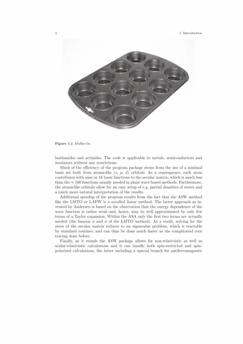
As all other augmentation schemes the ASW method is built upon the muffin-tinapproximation (MTA), which approximates the full crystal potential by sphericallysymmetric potential wells inside the non-overlapping muffin-tin spheres and a con-stant in the remaining, interstitial region. This situation resembles that of a muffin-tin as it is sketched in Fig. 1.1. Yet, the ASW method, like the LMTO method,is based on a special form of the MTA, namely, the atomic sphere approximation(ASA) as invented by Andersen, which is characterized by the requirement thatthe sum of all atomic spheres inside the unit cell has the same volume as that cell.Inside the spheres the potential as well as the electron densities (core and valence)are assumed to be spherical symmetric. While this socalled shape approximationof both the MTA and the ASA might seem as too crude an approximation to thefull crystal potential the ASA actually is not. This can be readily understood fromthe fact that the ASA condition creates overlap regions along the bond paths justbetween two atoms. In these regions the superposition of the two ASA potentials ex-periences an effective downshift as compared to the potentials of the single spheresand thus mimics the full potential quite well. Indeed, electronic properties calcu-lated using ASA based methods can hardly be distinguished from those growingout of the much more elaborate full potential methods.
However, due to the spherical symmetry and the overlap of the potential wellscalculated total energies still lack the accuracy needed e.g. for calculating elasticproperties or phonon frequencies. For this reason, I have implemented the new fullpotential version, which is now available for the first time.
As an all-electron scheme the ASW method fully includes both the core and thevalence electrons in the self-consistent field calculations. For this reason, it allowsfull coverage of the periodic table including transition metal atoms as well as the
4 1 Introduction
Figure 1.1 Muffin-tin.
lanthanides and actinides. The code is applicable to metals, semiconductors andinsulators without any restrictions.
Much of the efficiency of the program package stems from the use of a minimalbasis set built from atomiclike (s, p, d) orbitals. As a consequence, each atomcontributes with nine or 16 basis functions to the secular matrix, which is much lessthan the ≈ 100 functions usually needed in plane wave based methods. Furthermore,the atomiclike orbitals allow for an easy setup of e.g. partial densities of states anda much more natural interpretation of the results.
Additional speedup of the program results from the fact that the ASW methodlike the LMTO or LAPW is a socalled linear method. The latter approach as in-vented by Andersen is based on the observation that the energy dependence of thewave function is rather weak and, hence, may be well approximated by only fewterms of a Taylor expansion. Within the ASA only the first two terms are actuallyneeded (the famous φ and φ of the LMTO method). As a result, solving for thezeros of the secular matrix reduces to an eigenvalue problem, which is tractableby standard routines, and can thus be done much faster as the complicated roottracing done before.
Finally, as it stands the ASW package allows for non-relativistic as well asscalar-relativistic calculations and it can handle both spin-restricted and spin-polarized calculations, the latter including a special branch for antiferromagnetic

1.2 Physical background 5
order. Much work has been put into the code for accelerating the iterations towardsself-consistency.
Last not least, due to the implementeation of the sphere geometry optimization(SGO) algorithm the ASW programs allow for considering closed-packed systems aswell as rather open crystal structures. The SGO algorithm performs an automaticsphere packing including the generation of additional augmentation sphere positionsand the determination of optimal atomic sphere radii for use with the ASA.
Readers interested in a more detailed account of the ASW method are referredto my book [404].
Over the years more and more physical and chemical properties have becomeavailable by the ASW program package. Among them are the following.
• Electronic Properties
– electronic dispersions E(k) (“band structure“)– electronic wave functionsWave function ψ(k) =
∑
i ciHi(k)→ projected band structure
– total/partial (site/state projected) densities of states (DOS)– Fermi surface– electron densities– Laplacians of the electron density– Bader analysis of the electron density– electric field gradients– charge densities at the nuclei → isomer shifts– core level spectra
• Cohesive and Elastic Properties
– cohesive energy– bulk modulus– elastic constants– phonon frequencies
• Chemical Bonding
– total/partial crystal orbital overlap population (COOP), total/partial crystalorbital Hamiltonian population (COHP), total/partial covalence energy (Ecov)
• Magnetic Properties
– total and site/state projected magnetic moments– magnetic ordering (ferro-, ferri-, antiferromagnetic)– magnetic energies– spin densities– spin densities at the nuclei → hyperfine fields
• Optical Properties

6 1 Introduction
– plasma frequency– optical conductivity– dielectric function– index of refraction– extinction coefficient– optical reflectivity– optical absorption– energy-loss function
• Transport Properties
– electrical conductivity– electrical resistivity– thermopower– thermoelectric power factor– thermoelectric figure of merit– thermal conductivity (electronic contribution only)– Hall conductivity– Hall coefficient
Suggestions for additional properties, which should be implemented are always wel-come. Just sent an email to the address given above.
1.3 Programming
At present, the ASW program package consists of ≈ 120000 lines of source code,which are organized in a dozen main programs and about 450 subroutines. Whilethe first versions were written in FORTRAN 77, the latest versions have been fullyadapted to the Fortran 95 standard. In particular, extensive use of dynamic mem-ory now makes the package much faster and more flexible than before. Moreover,switching to Fortran 95 has enhanced portability of the code considerably.
In setting up prior versions of the program I have much benefitted from ftnchek,a public domain syntax checker for Fortran programs. Unfortunetely, ftnchek is nolonger developed and, in particular, can not be applied to Fortran 95 code.
As it stands the ASW program package is fully self-contained without the need tolink any library. Standard linear algebra tasks are handled by use of the LAPACKlibrary. For plotting the calculated data the programs provide interfaces to Gnuplot,RasMol, and XCrysDen, which are all public domain software. As a consequence,commercial libraries are not needed at all.
Finally, the program is fully portable to and has been tested on a large varietyof platform and with many compilers including
• IBM RS6000 (XL Fortran 95)• HP 9000 (Fortran 90)• CRAY Y-MP, YEL, J90, T90 (CF90)

1.4 Installation 7
• SGI (f90)• SNI S400 (frt), VPP500 (frtpx)• Sun SPARC (Solaris, f90)• Convex (ConvexOS, fc -f90)• Compaq Alpha (Fortran 95)• Power Mac G5 Mac OS X (G95)• PC (AMD/Intel) (Lahey/Fujitsu Fortran 95, PGI f90, Absoft Pro Fortran, NAG
f95, Intel f95)• All platforms: G95, GNU Fortran 95
For this reason, installing the package poses no problems and can be done within afew minutes.
Last but not least, in order to facilitate running the programs on larger machinesthe package includes shell scripts for use with the most common job queuing systemsas there are
• IBM’s LoadLeveler• Portable Batch System - PBS• Sun Grid Engine - SGE
1.4 Installation
Installation of the ASW package proceeds along two different lines. Usually, theexecutables and shell scripts are sent as a tarball. In this case the following stepshave to be performed.
1. Unpack the tarball by typing gunzip aswbin 2.5.tar.gz and tar -xvf aswbin 2.5.tar,which creates a subdirectory aswbin 2.5. This subdirectory contains
• all the executable (files mn*.run, pl*.run)• all shell scripts (files mn*.x, pl*.x, pl*.lx, and some more)• all the information files (README, COPYRIGHT, NEW2.5, HELP, SPC-
GRP)
2. Include this directory into your PATH settings.3. As a very first test you may type the command mnmpr.run, which generates a
one-page output of machine parameters (see Sec. 3.1) and proves the correctfunctionality of the executables.
4. From within the subdirectory aswbin 2.5, invoke the shell script upshl, whichwrites the correct path to all other shell scripts. As a consequence, the shellscripts can be called from any directory and they will call the correct executables.
5. Have fun running the ASW codes!
The alternative route starts from the source code. In this case these files firstmay have to be extracted from a tarball in a manner similar to the proceduredescribed above. Since the ASW package has been written with portability in mind,
8 1 Introduction
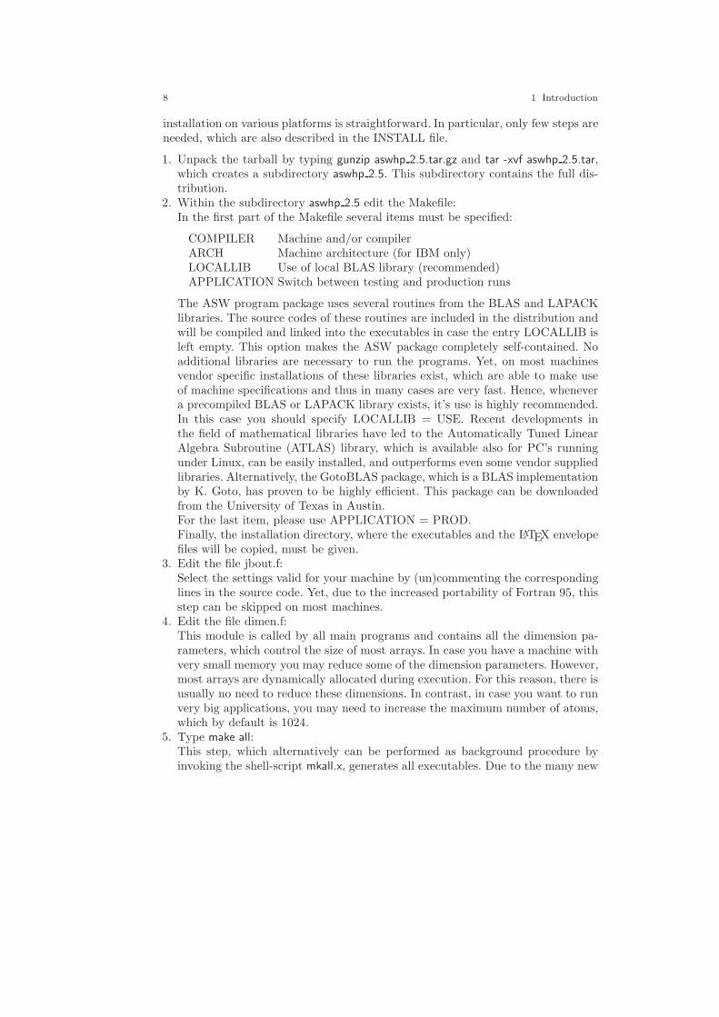
installation on various platforms is straightforward. In particular, only few steps areneeded, which are also described in the INSTALL file.
1. Unpack the tarball by typing gunzip aswhp 2.5.tar.gz and tar -xvf aswhp 2.5.tar,which creates a subdirectory aswhp 2.5. This subdirectory contains the full dis-tribution.
2. Within the subdirectory aswhp 2.5 edit the Makefile:In the first part of the Makefile several items must be specified:
COMPILER Machine and/or compilerARCH Machine architecture (for IBM only)LOCALLIB Use of local BLAS library (recommended)APPLICATION Switch between testing and production runs
The ASW program package uses several routines from the BLAS and LAPACKlibraries. The source codes of these routines are included in the distribution andwill be compiled and linked into the executables in case the entry LOCALLIB isleft empty. This option makes the ASW package completely self-contained. Noadditional libraries are necessary to run the programs. Yet, on most machinesvendor specific installations of these libraries exist, which are able to make useof machine specifications and thus in many cases are very fast. Hence, whenevera precompiled BLAS or LAPACK library exists, it’s use is highly recommended.In this case you should specify LOCALLIB = USE. Recent developments inthe field of mathematical libraries have led to the Automatically Tuned LinearAlgebra Subroutine (ATLAS) library, which is available also for PC’s runningunder Linux, can be easily installed, and outperforms even some vendor suppliedlibraries. Alternatively, the GotoBLAS package, which is a BLAS implementationby K. Goto, has proven to be highly efficient. This package can be downloadedfrom the University of Texas in Austin.For the last item, please use APPLICATION = PROD.Finally, the installation directory, where the executables and the LATEX envelopefiles will be copied, must be given.
3. Edit the file jbout.f:Select the settings valid for your machine by (un)commenting the correspondinglines in the source code. Yet, due to the increased portability of Fortran 95, thisstep can be skipped on most machines.
4. Edit the file dimen.f:This module is called by all main programs and contains all the dimension pa-rameters, which control the size of most arrays. In case you have a machine withvery small memory you may reduce some of the dimension parameters. However,most arrays are dynamically allocated during execution. For this reason, there isusually no need to reduce these dimensions. In contrast, in case you want to runvery big applications, you may need to increase the maximum number of atoms,which by default is 1024.
5. Type make all:This step, which alternatively can be performed as background procedure byinvoking the shell-script mkall.x, generates all executables. Due to the many new

1.5 Linking with external software 9
features incorporated in the Makefile its execution might require GNU make,which is free software and available from many servers, e.g. www.gnu.org.
6. Type make install:This copies all executables, shell-scripts and LATEX envelope files to the directoryspecified in step 1 above.
7. Have fun running the ASW codes!
In addition to the above steps the following make commands are useful.
• make clean:This command will remove all listing files possibly created by the compiler or byany of the syntax checkers as, e.g. ftnchek or forcheck. However, it will not affectany of the object files or any of the executables.
• make realclean:This command will remove all module and objects files as well as all executablesin addition to the listing files possibly created by the compiler or by any of thesyntax checkers.
1.5 Linking with external software
As it stands, the ASW program package delegates several tasks to specialized soft-ware. This holds especially for linear algebra problems and visualization of theresults.
The following software can be combined with the ASW package. This meansthat the Makefile and the programs themselves are perpared to be linked with thesoftware listed below. In particular, the plot routines provide the correspondinginterfaces and the programs write data files in the specific formats required by theexternal viausalization tools. To be specific, crystal structure and Fermi surfacedata as well as electron densities and related quantities are written in a format,which can be directly used by XCrysDen. Finally, many of the shell script used forplotting include a call to the corresponding external software.
All software included in the following list is public domain software. However,please do not forget referencing the particular software in publications in case youare asked for in order to appreciate the work of those who provide it.
ftnchek
(http://www.dsm.fordham.edu/∼ftnchek/)
A most valuable tool during several stages of the development of the ASW pack-age was ftnchek (short for ForTraN CHEcKer), which was developed by Robert

10 1 Introduction
Moniot at Fordham University. ftnchek is a syntax analyzer for FORTRAN 77 pro-grams. In addition, it has a special branch for the construction of calling trees forlarge program packages.
The Makefile of the ASW program package is prepared for working with ftnchek.However, development of ftnchek never went beyond FORTRAN 77. For this reason,after switching to Fortran 95, I have never used it any more.
BLAS/LAPACK
(http://www.netlib.org/blas/, http://www.netlib.org/lapack/)
BLAS and LAPACK have eveloved as THE standard software for solving linearalgebra problems. While basic linear algebra tasks are deferred to the BLAS (BasicLinear Algebra Subroutines), LAPACK provides a number of high level driver rou-tines, which grew out of a combination of its predecessors LINPACK and EISPACK.
However, all BLAS and LAPACK routines needed by the ASW software arealready included in the ASW program package. This makes the distribution self-contained and allows to compile the ASW programs without any need to downloadthe source codes of these libraries.
In addition, since LAPACK has become a de facto standard, the library is in-cluded in many Linux distributions. Furthermore, most machine dependent andvendor provided libraries as, e.g. ESSL by IBM have adopted the LAPACK callingsequences. Since these libraries are often very efficient it is recommended not to usethe BLAS/LAPACK sources coming with the ASW distribution, but to link withthe machine libraries.
ATLAS
(http://math-atlas.sourceforge.net/)
The ATLAS (Automatically Tuned Linear Algebra Software) provides a com-bined effort to supply LAPACK software with optimal tuning for a given machinearchitecture. To this end, ATLAS performs an extended check of systems resources,the result of which is transferred to the software in terms of, e.g. optimal block sizesof matrices. All this is done completely automatic and leads to a highly optimizedLAPACK library for a given machine.

1.5 Linking with external software 11
GotoBLAS
(http://www.tacc.utexas.edu/resources/software/)
Some years ago, K. Goto from the University of Texas in Austin provided anew implementation of BLAS/LAPACK, which outperforms the classical softwarein several cases. This is achieved by a more efficient use of memory mainly.
Gnuplot
(http://www.gnuplot.info/)
This is one of the classical tools for visualization.
XCrysDen
(http://www.xcrysden.org/)
This software was developed by A. Kokalj at the Jozef Stefan Institute in Ljubl-jana [405]. While the first version was still commercial, the code has been madepublic domain more recently. According to the website XCrySDen is a crystallineand molecular structure visualisation program, which aims at display of isosurfacesand contours, which can be superimposed on crystalline structures and interactivelyrotated and manipulated. It can run on most UNIX platforms, without any specialhardware requirements.
In the last years, XCrysDen has found much appreciation in the communityand on my opinion it is one of the best programs for displaying crystal structures,electron densities and related quantities, and Fermi surfaces.
RasMol
(http://www.rasmol.org/)
Another plot program going together with the ASW package is RasMol, whichwas developed by Roger A. Sayle. RasMol is used for plotting crystal structuresand reads files created by the plot program plstr.run. RasMol is also public domainand like Gnuplot it usually comes along with the standard Linux distributions.However, since this software was originally designed to visualize large molecules it is

12 1 Introduction
somewhat weak at display periodic systems and does not provide much functionalityfor crystals.
1.6 Legal matters
Since the ASW program package is also commercially distributed legal matters haveto be considered. Most of this is contained in the file COPYRIGHT coming withthe distribution, which is printed here for completeness.
**********************************************************************
*** ASW software package ***
**********************************************************************
*** Version 2.6 ***
**********************************************************************
*** Copyright notice ***
**********************************************************************
**********************************************************************
The ASW software package was written by Volker Eyert.
In setting up the package the author has benefitted from
experience gained during stays at the following institutes:
Institut fuer Festkoerperphysik, TH Darmstadt,
Hochschulstr. 6, 64289 Darmstadt, Germany
Institut fuer Physikalische Chemie, TH Darmstadt,
Petersenstr. 20, 64287 Darmstadt, Germany
Max-Planck-Institut fuer Festkoerperforschung,
Heisenbergstr. 1, 70569 Stuttgart, Germany
Hahn-Meitner-Institut,
Glienicker Str. 100, 14109 Berlin, Germany
Institut fuer Physik, Universitaet Augsburg,
Universitaetsstr. 1, 86135 Augsburg, Germany
**********************************************************************
Version ASW-2.6 15.01.2009 Volker Eyert
Copyright (C) 1992-2009 Volker Eyert
**********************************************************************
General:
Here and in the following the term "the author" refers to Volker Eyert
at the last of the above adresses.
You can contact the author via normal mail to the last of the above
adresses or via email to:
Here and in the following the term "ASW software package" refers to the
1.7 Upward compatibility 13
total of all files contained in the distribution (in source and object
form).
Here and in the following the term "core of the ASW software package"
refers to the total of all files contained in the distribution (in
source and object form) except for those files which explicitly contain
a copyright notice by other authors and except for the LAPACK and BLAS
routines coming with the distribution.
**********************************************************************
Copyright notice:
The core of the ASW software package is copyrighted software.
It is not allowed to change any of the copyright notices in the core
of the ASW software package.
It is not allowed to redistribute the core of the ASW software package
or any part of it without prior written permission of the author.
It is not allowed to incorporate any part of the core of the ASW software
package into any other software without prior written permission of the
author.
It is illegal to commercially distribute the core of the ASW software
package as a whole or any part of it or to incorporate any part of it
into a commercial product without prior written permission of the
author.
**********************************************************************
Disclaimer:
The ASW software package is distributed in the hope that it will be
useful, but WITHOUT ANY WARRANTY; without even the implied warranty
of MERCHANTIBILITY or FITNESS FOR A PARTICULAR PURPOSE.
**********************************************************************
1.7 Upward compatibility
In general, upward compatibility is guaranteed by the program. It is controlled bythe token ASW- in category VERSION of the CTRL file. For this reason, one should
14 1 Introduction
be careful in changing this token by hand. After reading the CTRL file the programsperform a complex check of the atomic files. This includes a check of the version ofthe code, which had written these files.
However, especially the transition from the old ASA-based versions (up to version1.9) to the full-potential versions (gradually starting from version 2.0) requiredmany changes in the underlying theory. In particular, the electron density and allrelated quantities now included also the non-spherical contribution inside the atomicspheres. As a consequence, the structure of the atomic files had to be changedcompletely and I decided to break the upwards compatibility rule. Hence, atomicfiles generated by programs prior to version 2.0 can no longer be used as input toprograms with version 2.0 and higher.
An important issue of upward compatibility regards the interpretation of theatomic coordinates coming with the CTRL file. To be specific, the interpretationof the relative atomic coordinates has been changed in a major revision in version2.1. Whereas in all program versions prior to this version relative coordinates (forswitch CARTP=F) were referred to the primitive translation they are now referredto the translations of the conventional cell, as is usual in crystallography. While thismakes the setup much more comfortable it leads to difficulties if old CTRL files arestill to be used. For this reason, I have implemented the following rule: If an oldCTRL file, i.e. a CTRL file generated by a version prior to version 2.1, is to be usedwith the atomic positions given in relative coordinates in terms of the primitivetranslations, then the old version number should be specified with the token ASW-in category VERSION. In other words, whenever the program reads a CTRL filewith the version number lower than 2.1, it interpretes the relative coordinates interms of the primitive translations rather than the translations of the conventionalcell.
1.8 Known bugs
So far the following bug is known, which has not yet been removed from the code:
1. The packing program mnpac.run was originally designed for the spin-degeneratecase only. As a consequence, it produces wrong results if NSPIN=2 is specifiedin the CTRL file. Please make sure that NSPIN=1 in the CTRL file or that thistoken is missing at all.

Chapter 2
Execution of the ASW programs: Casestudies
In the present chapter we will discuss how the ASW package can be used in anoptimal way. In doing so, we will apply the programs to several representative testcases, namely Cu, Si, FeS2, CrO2, and Gd.
In passing we mention that the total CPU time for all calculations described inthe chapter was about 48,000 sec on an Intel Pentium Mobile with 2.0GHz.
2.1 A simple case: Cu
Elemental copper has been used as a test case for electronic structure programs sincelong. This is for several reasons. As we will learn below, the electronic structureof this metal is strongly influenced by three groups of electrons. While the coreelectrons are tightly bound to the nucleus and, hence, have a very high electrondensity at the center of the atom but an almost negligible density in the outerregion, the wave functions of the 4s and 4p valence electrons reach far out andspread even into the region of neighbouring atoms. Finally, the 3d valence electronsare somewhat intermediate in that they likewise contribute to the overlap withneighbouring atoms, hence, to the metallic bonding but still are rather well localizednear the nuclei. Since the 3d states of copper are almost filled they contribute onlyweakly to the Fermi surface, which is therefore formed mostly by the 4s and 4pstates. As a consequence, although the 3d states are found well below EF anychanges or errors in the 4sp–3d overlap strongly affect the Fermi surface. For thisreason, copper is regarded as a sensitive test case. Calculated electronic structuresfor this material were compared to the results of photoemission experiments alreadyin the early 1960’s by Burdick [406].
The following calculations proceed in several steps. First we have to set up theCTRL file, which is the only input file for the calculations. All other files neededduring the execution of the programs are created automatically and auxiliary filesare deleted in case the programs do not need them any more. Once the self-consistentcalculation has converged, additional main programs may be invoked to evaluate the
15

16 2 Execution of the ASW programs: Case studies
band structure, the partial DOS, or the Fermi surface. Finally, the plot programscan be used to visualize the results.
In order to prepare for the calculations, we start creating a directory, where allthe files should be stored, by typing
mkdir cucd cumkdir nmcd nm
at the operating systems prompt. This creates a directory named cu with a subdirec-tory named nm, where nm stands for non-magnetic. This directory will hold all filesconnected with the particular application. Specifically, it will hold the CTRL file,which is the one and only input file to all ASW programs and has to be generatedat the very beginning.
2.1.1 CTRL file
Let us start by listing a minimum CTRL file for Cu, which you may either writefrom scratch or copy from the example file database. In case you write it yourselfremember not to use tabulators. On opening the CTRL file with your favorite editoryou will see the following.
HEADER Cu fcc
data by Landolt-Boernstein
VERSION ASW-2.6
STRUC ALAT=6.83079 CNTR=F
CLASS ATOM=CU Z=29
SITE ATOM=CU POS= 0.0 0.0 0.0
Each CTRL file is grouped into categories, which begin with a keyword atthe beginning of a line. In the above listing, five categories are identified, namelyHEADER, VERSION, STRUC, CLASS, and SITE. Each category comprises ad-ditional information, which, except for the first category, is passed to the programby socalled tokens. With the one and only exception being ASW-, these tokenshave the form TOKEN=, followed by one or more integer numbers, real numbers,character strings or logical switches (T or F). To be specific, in the present exam-ple the category STRUC contains all information about the Bravais lattice in formof the lattice constant, ALAT=6.83079 and the centering type, namely, CNTR=F(face-centered). While this fixes the unit cell of the crystal, information about thegeometry inside the unit cell is contained in the category SITE, which gives thepositions of all atoms. In the present case, only one atom exists, which is located atthe origin. This atom is labelled by ATOM=CU. Finally, the types of all atoms haveto be specified. This is done in category CLASS, where each atom via its label isassigned an atomic number. In the present case, there is only one atom with atomic

2.1 A simple case: Cu 17
number 29. Note that the label CU could be replaced by anything else. However,the program assumes that labels will not exceed six characters.
Finally, the category HEADER holds space for up to 20 lines of text for user com-ments. However, note that the first line (the one containing the keyword HEADER)is exceptional as by default its entry is used as a title line for all plots. Last notleast, category VERSION specfies the version of the program, which has generatedthe file or, if you have written the CTRL file from scratch, the version to be used.
While the above CTRL file already allows for a complete calculation a standardCTRL file may look as follows.
HEADER Cu fcc
data by Landolt-Boernstein
VERSION ASW-2.6
IO HELP=F SHOW=T VERBOS=30 CLEAN=T
OPTIONS REL=T OVLCHK=T
STRUC ALAT=6.83079 CNTR=F
CLASS ATOM=CU Z=29 R=2.6694476 LMXL=2 CONF=4 4 3 4 COORB=0 1 2
QVAL= 1.0 0.0 10.0 0.0
SITE ATOM=CU POS= 0.0 0.0 0.0
SYMGRP
ENVEL EKAP=-0.015
BZSMP NKBAB=6 BZINT=LTM EMIN=-1.0 EMAX=1.5 NDOS=2500
NORD=5 WIDTH=0.02 SAVDOS=F SAVCOOP=F SAVFERM=F SAVOPT=F
CHARGE NETA=2 EETA=-3.0 -5.0 SAVRHO=F
CONTROL START= QUIT= FREE=F NITBND=99 CNVG=1.0D-08 CNVGET=1.0D-08
NITATM=50 CNVGQA=1.0D-10
MIXING NMIXB=5 BETAB=0.5 INCBB=T NMIXA=5 BETAA=0.5
SYMLIN NPAN=5 NPTS=400 ORBWGT=T CARTE=F
LABEL=W ENDPT= 0.500 0.250 0.750
LABEL=L ENDPT= 0.500 0.500 0.500
LABEL=g ENDPT= 0.000 0.000 0.000
LABEL=X ENDPT= 0.500 0.000 0.500
LABEL=W ENDPT= 0.500 0.250 0.750
LABEL=K ENDPT= 0.375 0.375 0.750
PLOT CARTV=T
ORIGIN= 0.0 0.0 0.0
RPLOT1= 1.0 0.0 0.0
RPLOT2= 0.0 1.0 0.0
RPLOT3= 0.0 0.0 1.0
NPDIV1=50 NPDIV2=50 NPDIV3=00
It contains a lot more categories and tokens, all of which are discussed in detailin Chap. 4. Here we mention, in particular, the switch to scalar-relativistic calcu-lations, REL=T, the types of orbitals used in the calculations as specified by themaximum angular momentum, LMXL=2, the principal quantum numbers of all or-bitals CONF=4 4 3 4, and the respective orbital occupations QVAL=. . . . In caseyou are in doubt about the input for these three tokens just omit them. The pro-gram will add them for you. Moreover, we have specified the number of k-points tobe used in the Brillouin zone integration by the token NKBAB=6, which gives thenumber of k-points per inverse Bohr radii along each of the translation vectors ofthe reciprocal unit cell (see Chap. 4). Finally, the categories SYMLIN and PLOT,

18 2 Execution of the ASW programs: Case studies
respectively, hold information about the lines within the first Brillouin zone to beused for the band structure, and the region in real space used for plotting the crystalstructure as well as the electron density and potential.
Note that all entries given in the standard CTRL file above, which go beyondthose contained in the minimum CTRL file, reflect the default values. For thisreason, they do not need to be specified at all. In this context, two tokens are veryhelpful. First, by setting HELP=T in category IO and running any of the manyprograms mn*.run (except for mnmpr.run) a file named HELP is created, whichcontains a short description of every token. At the same time, an extended copyof the CTRL file, which includes all possible tokens with their default values, iswritten to standard output. Alternatively, for HELP=F and VERBOS=40 (or avalue greater than that) the program, besides executing its proposed task createsa file named CALL at the very end, which also contains an extended copy of theCTRL file.
2.1.2 Execution of the main programs
Once you have generated the CTRL file, the ASW program for self-consistent fieldcalculations can be started by typing
mnscf.run
at the operating systems prompt. However, for Unix/Linux systems the distributionoffers several useful shell scripts. Here, we just type
mnscf.x
at the systems prompt to start a job with the output sent to file outscf. The programwill use about 13 iterations to full convergence. On a standard PC the total exe-cution time will be about one second per interation. After completion, the outputfile outscf contains all the information collected during the iterations. In addition,a file named CU (the naming is due to the token ATOM= in categories CLASSand SITE) has been created, which contains all information specific to the respec-tive atom. These data are needed by the program. For this reason, you should notdelete an atomic file or change it by hand. Otherwise the program might have tostart from scratch again. All main programs have a complex file checking routineincluded, which detects the status of all atomic files and after that decides aboutthe action to be taken. In particular, this file check will stop execution in case youintend to start from scratch while converged atomic files are detected.
Once self-consistency has been achieved you are able to calculate the band struc-ture by typing
mnbnd.run
or, better,
mnbnd.x

2.1 A simple case: Cu 19
This program uses the information contained in the files CTRL and CU and gen-erates a new file called BNDE, which comprises the eigenvalues for each k-point,hence, the band structure. Output is stored in file outbnd, calculation of the bandstructure will take about half a second.
In addition, after having changed SAVDOS=F to SAVDOS=T as well as QUIT=to QUIT=BND and running mnscf.run again, you will obtain a file DOS, which holdsall information about the partial densities of states for plotting. The same can beachieved by invoking the shell script
mndos.x
which does the neccessary changes in the CTRL file (and resets to the original stateat the end) and writes output to file outdos.
Furthermore, in case the tokens SAVCOOP=F and SAVFERM=F are includedin category BZSMP, the same run creates the files COOP and FERM, which holdinformation about the chemical bonding indicators and the Fermi surface.
The total of the previous calculations can be made automatic by using the shellscript mnall.x. On typing
mnall.x
this shell script performs a self-consistent calculation for NKBAB=6 (this must beset in the CTRL file), then switches to NKBAB=12, and then to NKBAB=18. Foreach of these k-point grids a self-consistent calculation is performed. Note that thissaves a lot of execution time as compared to starting from scratch with a k-pointdensity of 18. This is due to the “restart” facility of the ASW program mnscf.run.Whenever the file checker in the program detects atomic files, which conform withthe general settings of the CTRL file as e.g. the lattice type or the number and typesof orbitals, the program is able to use this information as a starting point for furthercalculations. In particular, once the calculations for NKBAB=6 have convergedthe subsequent calculation for NKBAB=12 starts from the converged files ratherthan starting from scratch. As a result, only few iterations will be needed for fullconvergence at the higher k-space grid. Such a stepwise increase of the Brillouinzone density serves the additional purpose that on comparing the results we areable to check convergence of the result with respect to the fineness of the k-pointgrid. The results of all these calculations are stored in the files outlst6, outlst12, andoutlst18. Finally, the band structure, the (partial) densities of states, the bondingindicators, and possibly the Fermi surface are calculated.
In order to have a quick check of the progress of a self-consistent calculation justtype
monic outlst6
which will extract the following lines from the output file outlst6 and write them asa short summary to screen
ASW-2.6, program MNSCF started on asterix at Tue, 03 Feb 2009, 18:42:55.
Calculation converged after 13 iteration(s).
Start of Iteration 13
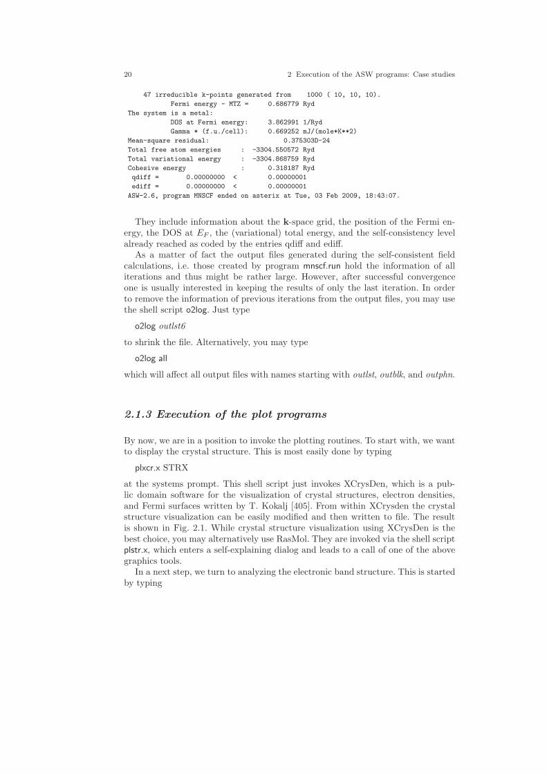
20 2 Execution of the ASW programs: Case studies
47 irreducible k-points generated from 1000 ( 10, 10, 10).
Fermi energy - MTZ = 0.686779 Ryd
The system is a metal:
DOS at Fermi energy: 3.862991 1/Ryd
Gamma * (f.u./cell): 0.669252 mJ/(mole*K**2)
Mean-square residual: 0.375303D-24
Total free atom energies : -3304.550572 Ryd
Total variational energy : -3304.868759 Ryd
Cohesive energy : 0.318187 Ryd
qdiff = 0.00000000 < 0.00000001
ediff = 0.00000000 < 0.00000001
ASW-2.6, program MNSCF ended on asterix at Tue, 03 Feb 2009, 18:43:07.
They include information about the k-space grid, the position of the Fermi en-ergy, the DOS at EF , the (variational) total energy, and the self-consistency levelalready reached as coded by the entries qdiff and ediff.
As a matter of fact the output files generated during the self-consistent fieldcalculations, i.e. those created by program mnscf.run hold the information of alliterations and thus might be rather large. However, after successful convergenceone is usually interested in keeping the results of only the last iteration. In orderto remove the information of previous iterations from the output files, you may usethe shell script o2log. Just type
o2log outlst6
to shrink the file. Alternatively, you may type
o2log all
which will affect all output files with names starting with outlst, outblk, and outphn.
2.1.3 Execution of the plot programs
By now, we are in a position to invoke the plotting routines. To start with, we wantto display the crystal structure. This is most easily done by typing
plxcr.x STRX
at the systems prompt. This shell script just invokes XCrysDen, which is a pub-lic domain software for the visualization of crystal structures, electron densities,and Fermi surfaces written by T. Kokalj [405]. From within XCrysden the crystalstructure visualization can be easily modified and then written to file. The resultis shown in Fig. 2.1. While crystal structure visualization using XCrysDen is thebest choice, you may alternatively use RasMol. They are invoked via the shell scriptplstr.x, which enters a self-explaining dialog and leads to a call of one of the abovegraphics tools.
In a next step, we turn to analyzing the electronic band structure. This is startedby typing
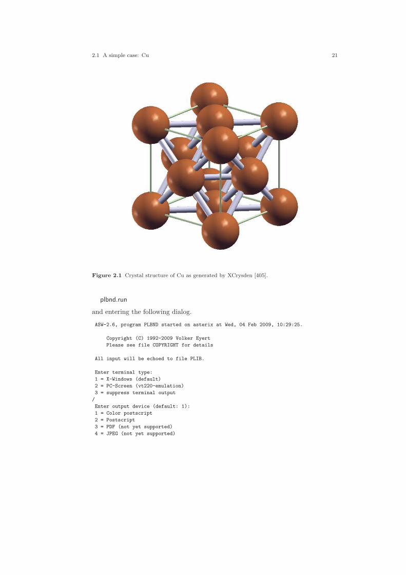
2.1 A simple case: Cu 21
Figure 2.1 Crystal structure of Cu as generated by XCrysden [405].
plbnd.run
and entering the following dialog.
ASW-2.6, program PLBND started on asterix at Wed, 04 Feb 2009, 10:29:25.
Copyright (C) 1992-2009 Volker Eyert
Please see file COPYRIGHT for details
All input will be echoed to file PLIB.
Enter terminal type:
1 = X-Windows (default)
2 = PC-Screen (vt220-emulation)
3 = suppress terminal output
/
Enter output device (default: 1):
1 = Color postscript
2 = Postscript
3 = PDF (not yet supported)
4 = JPEG (not yet supported)

22 2 Execution of the ASW programs: Case studies
5 = LaTeX
6 = LaTeX (special)
7 = HP LaserJet III (PCL5)
8 = PNG
9 = GIF
10 = leave decision for later
11 = suppress output to file
/
Portrait (P), landscape (L) or encapsulated postscript plot (E, default)?
/
Enter title:
/
Please wait a moment: I’m reading rest of file BNDE.
Timing for 39 points out of 398: 0.00000 sec.
Energies in Rydberg (F) or eV (T, default)?
/
Energies relative to MTZ (0) or EFermi (F, default)?
/
Energies connected by lines (T) (default F)?
/
Ebot = -9.737937 eV , Etop = 28.185740 eV relative to EF
Emin = -10.000000 eV , Emax = 6.000000 eV relative to EF
Enter new Emin, Emax to change these defaults:
/
task 1, total : cpu time: 0.04800 sec
ASW-2.6, program PLBND ended on asterix at Wed, 04 Feb 2009, 10:29:25.
Please delete files BNDE BNDV and bnd.ps bnd.tex when finished!!!
Here / entered on the programs prompt will keep the default values proposedby the program. All the questions are self-explaining. After this dialog, new fileshave been created, as there are BND.GNU, BND1, and BOX. By typing gnuplotBND.GNU you will invoke gnuplot and obtain the plot on screen. In addition, apostscript file bnd.ps is created, also containing the plot. For Cu the result is shownin Fig. 2.2. As we will discuss in more detail below, the band structure comprisesa parabolic band starting at the Γ -point at about −9.74 eV and ending near theW-point at 6 eV. This s-like band hybridizes with the five d-bands, which are visiblein the energy interval from −5.5 to −1.5 eV. Note the degeneracies of the d bandsespecially along the lines Γ -L and Γ -X.
Still the procedure can be simplified by calling the shell script plbnd.x rather thantyping plbnd.run. This will run the plot program and invoke Gnuplot automatically.Moreover, the intermediate files BND.GNU, BND1 and BOX will be deleted by theshell script at the very end.
However, user-friendlyness goes even beyond. During execution the plot routineplbnd.run has echoed all your input to a new file called PLIB. By inspecting thisfile you will find a fully commented echo of all your input. Rename this file to e.g.

2.1 A simple case: Cu 23
-10
-8
-6
-4
-2
0
2
4
6
W L Γ X W K
(E -
EF)
(eV
)
Cu fcc
Figure 2.2 Electronic structure of Cu along selected symmetry lines of the first Brillouin zone ofthe face-centered cubic lattice, see B.1.
PLIBf, type plbnd.x PLIBf, and you obtain the same result as before without havingto type anything else. This machinery could now be used to specify e.g. a differentenergy interval. Just edit file PLIBf and type plbnd.x PLIBf again. Yet, since filePLIB is just a simple echo, you should not change the order of the lines.
Next we are going to plot the partial densities of states. Now typing
pldos.x
you enter the following dialog.
ASW-2.6, program PLDOS started on asterix at Wed, 04 Feb 2009, 09:52:07.
Copyright (C) 1992-2009 Volker Eyert
Please see file COPYRIGHT for details
All input will be echoed to file PLID.
Enter terminal type:
1 = X-Windows (default)
2 = PC-Screen (vt220-emulation)
3 = suppress terminal output
/
Enter output device (default: 1):
1 = Color postscript
2 = Postscript
3 = PDF (not yet supported)
4 = JPEG (not yet supported)
5 = LaTeX
6 = LaTeX (special)
24 2 Execution of the ASW programs: Case studies
7 = HP LaserJet III (PCL5)
8 = PNG
9 = GIF
10 = leave decision for later
11 = suppress output to file
/
Portrait (P), landscape (L) or encapsulated postscript plot (E, default)?
Enter title:
/
Please wait a moment: I’m reading rest of file DOS.
Energies in Rydberg (F) or eV (T, default)?
/
Energies relative to MTZ (0) or EFermi (F, default)?
/
Energy axis to the top (F) or right (T, default)?
/
Plot DOS (F, default) or integrated DOS (T)?
/
Start setting up curve 1:
Plot partial (F) or total DOS (T, default)?
F
For partial DOS: Rotate reference frame for orbitals?
Enter rotation symbol (Default: E):
/
Enter orbital(s) to be included:
Class CU : atom 1 at 0.000000 0.000000 0.000000
Select from the following orbitals:
0: all -1: all p -2: all d -3: all f
1: s 2: y 3: z 4: x 5: xy
6: yz 7: 3z^2-r^2 8: xz 9: x^2-y^2 10: 3x^2y-y^3
11: xyz 12: 5yz^2-yr^2 13: 5z^3-3zr^2 14: 5xz^2-xr^2 15: x^2z-y^2z
16: x^3-3xy^2
1/
The following orbitals have been selected:
Class CU : atom 1, orbital s
Enter scaling factor (default 1.0):
/
Broadening of this curve (T) or not (F, default)?
Select curve style (default: 1) (A * marks styles already selected):
solid/green (1) , dash1/blue (2) ,
dash2/red (3) , dot/magenta (4) ,
dashdot1/cyan (5) , dashdot2/yellow (6) ,
chaindash1/black (7) , chaindash2/coral (8) ,
chaindash3/gray (9) ,
/
2.1 A simple case: Cu 25
Enter curve label ("/" to suppress)
Cu 4s
Please wait a moment: I’m working on this curve.
Set up more curves (T)? Default is F.
T
Start setting up curve 2:
Plot partial (F) or total DOS (T, default)?
F
For partial DOS: Rotate reference frame for orbitals?
Enter rotation symbol (Default: E):
/
Enter orbital(s) to be included:
Class CU : atom 1 at 0.000000 0.000000 0.000000
Select from the following orbitals:
0: all -1: all p -2: all d -3: all f
1: s 2: y 3: z 4: x 5: xy
6: yz 7: 3z^2-r^2 8: xz 9: x^2-y^2 10: 3x^2y-y^3
11: xyz 12: 5yz^2-yr^2 13: 5z^3-3zr^2 14: 5xz^2-xr^2 15: x^2z-y^2z
16: x^3-3xy^2
-1/
The following orbitals have been selected:
Class CU : atom 1, orbital y
Class CU : atom 1, orbital z
Class CU : atom 1, orbital x
Enter scaling factor (default 1.0):
/
Broadening of this curve (T) or not (F, default)?
/
Select curve style (default: 2) (A * marks styles already selected):
solid/green (1) * , dash1/blue (2) ,
dash2/red (3) , dot/magenta (4) ,
dashdot1/cyan (5) , dashdot2/yellow (6) ,
chaindash1/black (7) , chaindash2/coral (8) ,
chaindash3/gray (9) ,
/
Enter curve label ("/" to suppress)
Cu 4p
Please wait a moment: I’m working on this curve.
Set up more curves (T)? Default is F.
T
Start setting up curve 3:
Plot partial (F) or total DOS (T, default)?
26 2 Execution of the ASW programs: Case studies
F
For partial DOS: Rotate reference frame for orbitals?
Enter rotation symbol (Default: E):
/
Enter orbital(s) to be included:
Class CU : atom 1 at 0.000000 0.000000 0.000000
Select from the following orbitals:
0: all -1: all p -2: all d -3: all f
1: s 2: y 3: z 4: x 5: xy
6: yz 7: 3z^2-r^2 8: xz 9: x^2-y^2 10: 3x^2y-y^3
11: xyz 12: 5yz^2-yr^2 13: 5z^3-3zr^2 14: 5xz^2-xr^2 15: x^2z-y^2z
16: x^3-3xy^2
5
6
8/
The following orbitals have been selected:
Class CU : atom 1, orbital xy
Class CU : atom 1, orbital yz
Class CU : atom 1, orbital xz
Enter scaling factor (default 1.0):
/
Broadening of this curve (T) or not (F, default)?
/
Select curve style (default: 3) (A * marks styles already selected):
solid/green (1) * , dash1/blue (2) * ,
dash2/red (3) , dot/magenta (4) ,
dashdot1/cyan (5) , dashdot2/yellow (6) ,
chaindash1/black (7) , chaindash2/coral (8) ,
chaindash3/gray (9) ,
/
Enter curve label ("/" to suppress)
Cu 3d t_{2g}
Please wait a moment: I’m working on this curve.
Set up more curves (T)? Default is F.
T
Start setting up curve 4:
Plot partial (F) or total DOS (T, default)?
F
For partial DOS: Rotate reference frame for orbitals?
Enter rotation symbol (Default: E):
/
Enter orbital(s) to be included:
Class CU : atom 1 at 0.000000 0.000000 0.000000

2.1 A simple case: Cu 27
Select from the following orbitals:
0: all -1: all p -2: all d -3: all f
1: s 2: y 3: z 4: x 5: xy
6: yz 7: 3z^2-r^2 8: xz 9: x^2-y^2 10: 3x^2y-y^3
11: xyz 12: 5yz^2-yr^2 13: 5z^3-3zr^2 14: 5xz^2-xr^2 15: x^2z-y^2z
16: x^3-3xy^2
7
9/
The following orbitals have been selected:
Class CU : atom 1, orbital 3z^2-r^2
Class CU : atom 1, orbital x^2-y^2
Enter scaling factor (default 1.0):
/
Broadening of this curve (T) or not (F, default)?
/
Select curve style (default: 4) (A * marks styles already selected):
solid/green (1) * , dash1/blue (2) * ,
dash2/red (3) * , dot/magenta (4) ,
dashdot1/cyan (5) , dashdot2/yellow (6) ,
chaindash1/black (7) , chaindash2/coral (8) ,
chaindash3/gray (9) ,
/
Enter curve label ("/" to suppress)
3d e_g
Please wait a moment: I’m working on this curve.
Set up more curves (T)? Default is F.
/
Center of gravity of DOS curve 1 (Spin 1) - EF : 0.4947 eV
Center of gravity of DOS curve 2 (Spin 1) - EF : 1.9557 eV
Center of gravity of DOS curve 3 (Spin 1) - EF : -2.3726 eV
Center of gravity of DOS curve 4 (Spin 1) - EF : -2.5612 eV
Indicate center of gravities (F, default)?
/
Ebot = -9.727926 eV , Etop = 11.129600 eV relative to EF
Emin = -10.000000 eV , Emax = 6.000000 eV relative to EF
Enter new Emin, Emax to change the default:
/
DOStop = 4.710970 1/eV
DOSmax = 5.000000 1/eV
Enter new DOSmax to change this default:
/
Enter energetic position of curve labels ("/" to use default):
-4
task 1, total : cpu time: 0.03600 sec
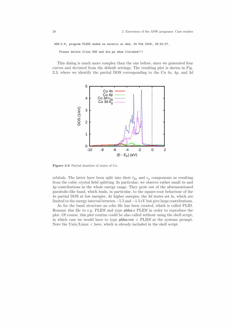
28 2 Execution of the ASW programs: Case studies
ASW-2.6, program PLDOS ended on asterix at Wed, 04 Feb 2009, 09:52:07.
Please delete files DOS and dos.ps when finished!!!
This dialog is much more complex than the one before, since we generated fourcurves and deviated from the default settings. The resulting plot is shown in Fig.2.3, where we identify the partial DOS corresponding to the Cu 4s, 4p, and 3d
0
1
2
3
4
5
-10 -8 -6 -4 -2 0 2
DO
S (
1/eV
)
(E - EF) (eV)
Cu 4sCu 4p
Cu 3d t2gCu 3d eg
Figure 2.3 Partial densities of states of Cu.
orbitals. The latter have been split into their t2g and eg components as resultingfrom the cubic crystal field splitting. In particular, we observe rather small 4s and4p contributions in the whole energy range. They grow out of the aforementionedparabolic-like band, which leads, in particular, to the square-root behaviour of the4s partial DOS at low energies. At higher energies, the 3d states set in, which arelimited to the energy interval between −5.5 and −1.5 eV but give large contributions.
As for the band structure an echo file has been created, which is called PLID.Rename this file to e.g. PLIDf and type pldos.x PLIDf in order to reproduce theplot. Of course, this plot routine could be also called without using the shell script,in which case we would have to type pldos.run < PLIDf at the systems prompt.Note the Unix/Linux < here, which is already included in the shell script.
2.1 A simple case: Cu 29
2.1.4 Advanced features
So far, we were able to decompose the total DOS into partial densities of states andwere thus able to identify orbital contributions in certain energy intervals. However,a corresponding analysis at a k-point level would be welcome. Such a tools existsin the ASW program package. In order to use it we enter the CTRL file and changein category SYMLIN the token NPTS=400 to NPTS=200 and ORBWGT=F toORBWGT=T. It is suggested to first copy the files CTRL and CU to a separatedirectory and do the changes of the CTRL file there. After having changed theCTRL file as described type mnbnd.x. As before this will produce a file BNDE. Inaddition, a file named BNDV is generated, which contains all the eigenvectors.
Next you invoke again the plotting shell script plbnd.x and enter the followingdialog.
ASW-2.6, program PLBND started on asterix at Wed, 04 Feb 2009, 10:16:03.
Copyright (C) 1992-2009 Volker Eyert
Please see file COPYRIGHT for details
All input will be echoed to file PLIB.
Enter terminal type:
1 = X-Windows (default)
2 = PC-Screen (vt220-emulation)
3 = suppress terminal output
/
Enter output device (default: 1):
1 = Color postscript
2 = Postscript
3 = PDF (not yet supported)
4 = JPEG (not yet supported)
5 = LaTeX
6 = LaTeX (special)
7 = HP LaserJet III (PCL5)
8 = PNG
9 = GIF
10 = leave decision for later
11 = suppress output to file
6
Portrait (P, default) or landscape plot (L)?
/
Enter title:
&, weighted $ 4s $
Please wait a moment: I’m reading rest of file BNDE.
Timing for 39 points out of 398: 0.00000 sec.
Energies in Rydberg (F) or eV (T, default)?
/
Energies relative to MTZ (0) or EFermi (F, default)?
/
Energies connected by lines (T) (default F)?

30 2 Execution of the ASW programs: Case studies
/
Plot orbital character (default F)?
T
For plotting orbital character: Rotate reference frame for orbitals?
Enter rotation symbol (E for unity):
/
Enter orbital(s) to be included:
Class CU : atom 1 at 0.000000 0.000000 0.000000
Select from the following orbitals:
0: all -1: all p -2: all d
1: s 2: y 3: z 4: x 5: xy
6: yz 7: 3z^2-r^2 8: xz 9: x^2-y^2
1
The following orbitals have been selected:
Class CU : atom 1, orbital s
Ebot = -9.737937 eV , Etop = 28.185740 eV relative to EF
Emin = -10.000000 eV , Emax = 6.000000 eV relative to EF
Enter new Emin, Emax to change these defaults:
/
Rescale orbital weights (default: 0.4000eV )?
/
Please wait a moment: I’m working on the weights.
Timing for 39 points out of 398: 0.00400 sec.
Enter the horizontal and vertical extension in mm.
Default: 100.0 x 90.0
/
task 1, total : cpu time: 0.23201 sec
ASW-2.6, program PLBND ended on asterix at Wed, 04 Feb 2009, 10:16:04.
Please delete files BNDE BNDV and bnd.tex when finished!!!
It differs from the above dialog by asking for
Plot orbital character (default f)?
and the particular orbital(s) to be included. This section is similar to the plottingof the partial DOS above. The previous dialog will produce a file bnd.tex, whichcan be converted into bnd.ps by typing plbnd.lx at the system prompt. The resultis shown in Fig. 2.4. In a similar way, orbital weighted band structures for the 4p,3dt2g, and 3deg states can be obtained. They are shown in Figs. 2.5, 2.6, and 2.7.In all these figures we recognize the same band structure as already given in Fig.2.2. Yet, in Figs. 2.4 to 2.7 to each band at each k-point has been appended a bar.The length of each bar is a measure of the contribution of a particular orbital to therespective wavefunction. To be specific, we identify large 4s and 4p contributionsat the bottom as well as at the high energy branches of the parabola starting at

2.1 A simple case: Cu 31
qqqqqqqqqqqqqqqqqqqqqqqqqqqqqqqqqqqqqqqqqqqqqqqqqqqqqqqqqqqqqqqqqqqqqqqqqqqqqqqqqqqqqqqqqqqqqqqqqqqqqqqqqqqqqqq
qqqqqqqqqqqqqqqqqqqqqqqqqqqqqqqqqqqqqqqqqqqqqqqqqqqqqqqqqqqqqqqqqqqqqqqqqqqqqqqq
qqqqqqqqqqqqqqqqqqqqqqqqqqqqqqqqqqqqqqqqqqqqqqqqqqqqqqqqqqqqqqqqqqqqqqqqqqqqqqqqqqqqqqqqqqqqqqqqqqqqqqqqqqqqqqqqqqq
qqqqqqqqqqqqqqqqqqqqqqqqqqqqqqqqqqqqqqqqqqqqqqqqqqqqqqqqqqqqqqqqqqqqqqqqqqqqqqqqqqqqqqqqqqqq
qqqqqqqqqqqqqqqqqqqqqqqqqqqqqqqqqqqqqqqqqqqqqqqqqqqqqqqqqqqqqqqqqqqqqqqqqqqqqqqqqqqqqqqqqqqqqqqqqqqqqq
qqqqqqqqqqqqqqqqqqqqqqqqqqqqqqqqqqqqqqqqqqqqqqqqqqqqqqqqqqqqqqqqqqqqqqqqqqqqq
qqqqqqqqqqqqqqqqqqqqqqqqqqqqqqqqqqqqqqqqqqqqqqqqqqqqqqqqqqqqqqqqqqqqqqqqqqqqqqqqqqqqqqqqqqqqqqqqqqqqqqqqqqqqqqqqqqqqqqqqqqqqqqqqqqqqqqqqqqqqqqqqqqqqqqqqqqqqqqqqqqqqqqqqqqqqqqqqqqqqqqqqqqqqqqqqqqqqqqqqqqqqqqqqqqqqqqqqqqq
qqqqqqqqqqqqqqqqqqqqqqqqqqqqqqqqqqqqqqqqqqqqqqqqqqqqqqqqqqqqqqqqqqqqqqqqqqqqqqqqqqqqqqqqqqqqqqqqqqqqqqqqqqq
qqqqqqqqqqqqqqqqqqqqqqqqqqqqqqqqqqqqqqqqqqqqqqqqqqqqqqqqqqqqqqqqqqqqqqqqqqqqqqqqqqqqqqqqqqqqq
qqqqqqqqqqqqqqqqqqqqqqqqqqqqqqqqqqqqqqqqqqqqqqqqq
qqqqqqqqqqqqqqqqqqqqqqqqqqqqqqqqqqq
qqqqqqqqqqqqqqqqqqqqqqqqqqqqqqqqqqqqqqqqqqqqqqqqqqqqqqqqqqqqqqqqqqqqqqqqqqqqqqqqqqqqqqqqqqqqqqqqqqqqqqqqqqqqqqqqqq
qqqqqqqqqqqqqqqqqqqqqqqqqqqqqqqqqqqqqqqqqqqqqqqqqqqqqqqqqqqqqqqqqqqqqqqqqqqqqqqqqqqqqqqqqqqqqq
qqqqqqqqqqqqqqqqqqqqqqqqqqqqqq
qqqqqqqqqqqqqqqqqqqqqqqqqqqqqqqqqqqqqqqqqqqqqqqqqqqqqqqqqqqqqqqqqqqqqqqqqqqqqqqqqqqqqqqqqqqqqqqqqqqqqqqqqqqqqqqqqqqqqqqqqqqqqqqqqqqqqqqqqqqqqqqqqqqqqqqqqqqqqqqqqqqqqqqqqqqqqqqqqqqqqqqqqqqqqqqqqqqqqqqqqqqqqqqqqqqqqqqqqqqqqqqqqqqqqqqqqqqqqqqqqqqqqqqq
qqqqqqqqqqqqqqqqqqqqqqqqqq
qqqqqqqqqqqqqqqqqqqqqqqqqqqqqqqqqqqqqqqqqqqqqqqqqqqqqqqqqqqqqqqqqqqqqqqqqqqqqqqqqqqqqqqqqqqqqqqqqqqqqqqqqqqqqqqqqqqqqqqqqqqqqqqqqqqqqqqqqqqqqqqqqqqqqqqqqqqqqqqqqqqqqqqqqqqqqqqqqqqqqqqqqqqqqqqqqqqqqqqqqqqqqqqqqqqqqqqqqqqqqqqqqqqqqqqqqqqqqqqqqqqqqqqqqqqqqqqqqqqqqqqqqqqqqqqqqqqqqqqqqqqqqqqqqqqqqqqqqqqqqqqqqqqqqqqqqqqqqqqqqqqqqqqqqqqqqqqqqqqqqqqqqqqqqqqqqqqqqqqqqqqqqqqqqqqqqqqqqqqqqqqqqqqqqqqqqqqqqq
qqqqqqqqqqqqqqqqqqqqqqqqqqqqqqqqqqqqqqqqqqqqqqqqqqqqqqqqqqqqqqqqqqqqqqqqqqqqqqq
qqqqqqqqqqqqqqqqqqqqqqqqqqqqqqqqqqqqqqqqqqqqqqqqqqqqqqqqqqqqqqqqqqqqqqqqqqqqqqqqqqqqqqqqqqqqqqqqqqqqqqqqqqqqq
qqqqqqqqqqqqqqqqqqqqqqqqqq
qqqqqqqqqqqqqqqqqqqqqqqqqqqqqqqqqqqqq
qqqqqqqqqqqqqqqqqqqqqqqqqqqqqqqqqqqqqqqqqqqqqqqqqqqqqqqqqqqqqqqqqqqqqqqqqqqqqqqqqqqqqqqq q
qqqqqqqqqqqqqqqqqqqqqqqqqqqqqqqq
qqqqqqqqqqqqqqqqqqqqqqqqqqqqqqqqqqqqqqqqqqqqqqqqqqqqqqqqqqqqqqqqqqqqqqq
qqqqqqqqq
q
q
q
q
q
Cu fcc, weighted 4s
W L Γ X W K
E
eV
EF
-10.0
-8.0
-6.0
-4.0
-2.0
0.0
2.0
4.0
6.0
Figure 2.4 Weighted electronic structure of Cu. The width of the bars given for each bandindicates the contribution due to the 4s orbital.
qqqqqqqqqqqqqqqqqqqqqqqqqqqqqqqqqqqqqqqqqqqqqqqqqqqqqqqqqqqqqqqqqqqqqqqqqqqqqqqqqqqqqqqqqqqqqqqqqqqqqqqqqqqqqqq
qqqqqqqqqqqqqqqqqqqqqqqqqqqqqqqqqqqqqqqqqqqqqqqqqqqqqqqqqqqqqqqqqqqqqqqqqqqqqqqq
qqqqqqqqqqqqqqqqqqqqqqqqqqqqqqqqqqqqqqqqqqqqqqqqqqqqqqqqqqqqqqqqqqqqqqqqqqqqqqqqqqqqqqqqqqqqqqqqqqqqqqqqqqqqqqqqqqq
qqqqqqqqqqqqqqqqqqqqqqqqqqqqqqqqqqqqqqqqqqqqqqqqqqqqqqqqqqqqqqqqqqqqqqqqqqqqqqqqqqqqqqqqqqqq
qqqqqqqqqqqqqqqqqqqqqqqqqqqqqqqqqqqqqqqqqqqqqqqqqqqqqqqqqqqqqqqqqqqqqqqqqqqqqqqqqqqqqqqqqqqqqqqqqqqqqq
qqqqqqqqqqqqqqqqqqqqqqqqqqqqqqqqqqqqqqqqqqqqqqqqqqqqqqqqqqqqqqqqqqqqqqqqqqqqq
qqqqqqqqqqqqqqqqqqqqqqqqqqqqqqqqqqqqqqqqqqqqqqqqqqqqqqqqqqqqqqqqqqqqqqqqqqqqqqqqqqqqqqqqqqqqqqqqqqqqqqqqqqqqqqqqqqqqqqqqqqqqqqqqqqqqqqqqqqqqqqqqqqqqqqqqqqqqqqqqqqqqqqqqqqqqqqqqqqqqqqqqqqqqqqqqqqqqqqqqqqqqqqqqqqqqqqqqqqq
qqqqqqqqqqqqqqqqqqqqqqqqqqqqqqqqqqqqqqqqqqqqqqqqqqqqqqqqqqqqqqqqqqqqqqqqqqqqqqqqqqqqqqqqqqqqqqqqqqqqqqqqqqq
qqqqqqqqqqqqqqqqqqqqqqqqqqqqqqqqqqqqqqqqqqqqqqqqqqqqqqqqqqqqqqqqqqqqqqqqqqqqqqqqqqqqqqqqqqqqq
qqqqqqqqqqqqqqqqqqqqqqqqqqqqqqqqqqqqqqqqqqqqqqqqq
qqqqqqqqqqqqqqqqqqqqqqqqqqqqqqqqqqq
qqqqqqqqqqqqqqqqqqqqqqqqqqqqqqqqqqqqqqqqqqqqqqqqqqqqqqqqqqqqqqqqqqqqqqqqqqqqqqqqqqqqqqqqqqqqqqqqqqqqqqqqqqqqqqqqqq
qqqqqqqqqqqqqqqqqqqqqqqqqqqqqqqqqqqqqqqqqqqqqqqqqqqqqqqqqqqqqqqqqqqqqqqqqqqqqqqqqqqqqqqqqqqqqq
qqqqqqqqqqqqqqqqqqqqqqqqqqqqqq
qqqqqqqqqqqqqqqqqqqqqqqqqqqqqqqqqqqqqqqqqqqqqqqqqqqqqqqqqqqqqqqqqqqqqqqqqqqqqqqqqqqqqqqqqqqqqqqqqqqqqqqqqqqqqqqqqqqqqqqqqqqqqqqqqqqqqqqqqqqqqqqqqqqqqqqqqqqqqqqqqqqqqqqqqqqqqqqqqqqqqqqqqqqqqqqqqqqqqqqqqqqqqqqqqqqqqqqqqqqqqqqqqqqqqqqqqqqqqqqqqqqqqqqq
qqqqqqqqqqqqqqqqqqqqqqqqqq
qqqqqqqqqqqqqqqqqqqqqqqqqqqqqqqqqqqqqqqqqqqqqqqqqqqqqqqqqqqqqqqqqqqqqqqqqqqqqqqqqqqqqqqqqqqqqqqqqqqqqqqqqqqqqqqqqqqqqqqqqqqqqqqqqqqqqqqqqqqqqqqqqqqqqqqqqqqqqqqqqqqqqqqqqqqqqqqqqqqqqqqqqqqqqqqqqqqqqqqqqqqqqqqqqqqqqqqqqqqqqqqqqqqqqqqqqqqqqqqqqqqqqqqqqqqqqqqqqqqqqqqqqqqqqqqqqqqqqqqqqqqqqqqqqqqqqqqqqqqqqqqqqqqqqqqqqqqqqqqqqqqqqqqqqqqqqqqqqqqqqqqqqqqqqqqqqqqqqqqqqqqqqqqqqqqqqqqqqqqqqqqqqqqqqqqqqqqqqq
qqqqqqqqqqqqqqqqqqqqqqqqqqqqqqqqqqqqqqqqqqqqqqqqqqqqqqqqqqqqqqqqqqqqqqqqqqqqqqq
qqqqqqqqqqqqqqqqqqqqqqqqqqqqqqqqqqqqqqqqqqqqqqqqqqqqqqqqqqqqqqqqqqqqqqqqqqqqqqqqqqqqqqqqqqqqqqqqqqqqqqqqqqqqq
qqqqqqqqqqqqqqqqqqqqqqqqqq
qqqqqqqqqqqqqqqqqqqqqqqqqqqqqqqqqqqqq
qqqqqqqqqqqqqqqqqqqqqqqqqqqqqqqqqqqqqqqqqqqqqqqqqqqqqqqqqqqqqqqqqqqqqqqqqqqqqqqqqqqqqqqq q
qqqqqqqqqqqqqqqqqqqqqqqqqqqqqqqq
qqqqqqqqqqqqqqqqqqqqqqqqqqqqqqqqqqqqqqqqqqqqqqqqqqqqqqqqqqqqqqqqqqqqqqq
qqqqqqqqq
q
q
q
q
q
Cu fcc, weighted 4p
W L Γ X W K
E
eV
EF
-10.0
-8.0
-6.0
-4.0
-2.0
0.0
2.0
4.0
6.0
Figure 2.5 Weighted electronic structure of Cu. The width of the bars given for each bandindicates the contribution due to the 4p orbitals.
−9.74 eV. In contrast the 3d orbitals dominate in the energy interval from −5.5 to−1.5 eV. These observations thus confirm our arguments put forward in the abovediscussion of the bare band structure and the partial densities of states. Actually,these orbital weighted band structures are a necessary prerequisite for a completeunderstanding of the electronic structure. Yet, only few band structure packagesoffer this analytical tool.

32 2 Execution of the ASW programs: Case studies
qqqqqqqqqqqqqqqqqqqqqqqqqqqqqqqqqqqqqqqqqqqqqqqqqqqqqqqqqqqqqqqqqqqqqqqqqqqqqqqqqqqqqqqqqqqqqqqqqqqqqqqqqqqqqqq
qqqqqqqqqqqqqqqqqqqqqqqqqqqqqqqqqqqqqqqqqqqqqqqqqqqqqqqqqqqqqqqqqqqqqqqqqqqqqqqq
qqqqqqqqqqqqqqqqqqqqqqqqqqqqqqqqqqqqqqqqqqqqqqqqqqqqqqqqqqqqqqqqqqqqqqqqqqqqqqqqqqqqqqqqqqqqqqqqqqqqqqqqqqqqqqqqqqq
qqqqqqqqqqqqqqqqqqqqqqqqqqqqqqqqqqqqqqqqqqqqqqqqqqqqqqqqqqqqqqqqqqqqqqqqqqqqqqqqqqqqqqqqqqqq
qqqqqqqqqqqqqqqqqqqqqqqqqqqqqqqqqqqqqqqqqqqqqqqqqqqqqqqqqqqqqqqqqqqqqqqqqqqqqqqqqqqqqqqqqqqqqqqqqqqqqq
qqqqqqqqqqqqqqqqqqqqqqqqqqqqqqqqqqqqqqqqqqqqqqqqqqqqqqqqqqqqqqqqqqqqqqqqqqqqq
qqqqqqqqqqqqqqqqqqqqqqqqqqqqqqqqqqqqqqqqqqqqqqqqqqqqqqqqqqqqqqqqqqqqqqqqqqqqqqqqqqqqqqqqqqqqqqqqqqqqqqqqqqqqqqqqqqqqqqqqqqqqqqqqqqqqqqqqqqqqqqqqqqqqqqqqqqqqqqqqqqqqqqqqqqqqqqqqqqqqqqqqqqqqqqqqqqqqqqqqqqqqqqqqqqqqqqqqqqq
qqqqqqqqqqqqqqqqqqqqqqqqqqqqqqqqqqqqqqqqqqqqqqqqqqqqqqqqqqqqqqqqqqqqqqqqqqqqqqqqqqqqqqqqqqqqqqqqqqqqqqqqqqq
qqqqqqqqqqqqqqqqqqqqqqqqqqqqqqqqqqqqqqqqqqqqqqqqqqqqqqqqqqqqqqqqqqqqqqqqqqqqqqqqqqqqqqqqqqqqq
qqqqqqqqqqqqqqqqqqqqqqqqqqqqqqqqqqqqqqqqqqqqqqqqq
qqqqqqqqqqqqqqqqqqqqqqqqqqqqqqqqqqq
qqqqqqqqqqqqqqqqqqqqqqqqqqqqqqqqqqqqqqqqqqqqqqqqqqqqqqqqqqqqqqqqqqqqqqqqqqqqqqqqqqqqqqqqqqqqqqqqqqqqqqqqqqqqqqqqqq
qqqqqqqqqqqqqqqqqqqqqqqqqqqqqqqqqqqqqqqqqqqqqqqqqqqqqqqqqqqqqqqqqqqqqqqqqqqqqqqqqqqqqqqqqqqqqq
qqqqqqqqqqqqqqqqqqqqqqqqqqqqqq
qqqqqqqqqqqqqqqqqqqqqqqqqqqqqqqqqqqqqqqqqqqqqqqqqqqqqqqqqqqqqqqqqqqqqqqqqqqqqqqqqqqqqqqqqqqqqqqqqqqqqqqqqqqqqqqqqqqqqqqqqqqqqqqqqqqqqqqqqqqqqqqqqqqqqqqqqqqqqqqqqqqqqqqqqqqqqqqqqqqqqqqqqqqqqqqqqqqqqqqqqqqqqqqqqqqqqqqqqqqqqqqqqqqqqqqqqqqqqqqqqqqqqqqq
qqqqqqqqqqqqqqqqqqqqqqqqqq
qqqqqqqqqqqqqqqqqqqqqqqqqqqqqqqqqqqqqqqqqqqqqqqqqqqqqqqqqqqqqqqqqqqqqqqqqqqqqqqqqqqqqqqqqqqqqqqqqqqqqqqqqqqqqqqqqqqqqqqqqqqqqqqqqqqqqqqqqqqqqqqqqqqqqqqqqqqqqqqqqqqqqqqqqqqqqqqqqqqqqqqqqqqqqqqqqqqqqqqqqqqqqqqqqqqqqqqqqqqqqqqqqqqqqqqqqqqqqqqqqqqqqqqqqqqqqqqqqqqqqqqqqqqqqqqqqqqqqqqqqqqqqqqqqqqqqqqqqqqqqqqqqqqqqqqqqqqqqqqqqqqqqqqqqqqqqqqqqqqqqqqqqqqqqqqqqqqqqqqqqqqqqqqqqqqqqqqqqqqqqqqqqqqqqqqqqqqqqq
qqqqqqqqqqqqqqqqqqqqqqqqqqqqqqqqqqqqqqqqqqqqqqqqqqqqqqqqqqqqqqqqqqqqqqqqqqqqqqq
qqqqqqqqqqqqqqqqqqqqqqqqqqqqqqqqqqqqqqqqqqqqqqqqqqqqqqqqqqqqqqqqqqqqqqqqqqqqqqqqqqqqqqqqqqqqqqqqqqqqqqqqqqqqq
qqqqqqqqqqqqqqqqqqqqqqqqqq
qqqqqqqqqqqqqqqqqqqqqqqqqqqqqqqqqqqqq
qqqqqqqqqqqqqqqqqqqqqqqqqqqqqqqqqqqqqqqqqqqqqqqqqqqqqqqqqqqqqqqqqqqqqqqqqqqqqqqqqqqqqqqq q
qqqqqqqqqqqqqqqqqqqqqqqqqqqqqqqq
qqqqqqqqqqqqqqqqqqqqqqqqqqqqqqqqqqqqqqqqqqqqqqqqqqqqqqqqqqqqqqqqqqqqqqq
qqqqqqqqq
q
q
q
q
q
Cu fcc, weighted 3dt2g
W L Γ X W K
E
eV
EF
-10.0
-8.0
-6.0
-4.0
-2.0
0.0
2.0
4.0
6.0
Figure 2.6 Weighted electronic structure of Cu. The width of the bars given for each bandindicates the contribution due to the 3dt2g orbitals.
qqqqqqqqqqqqqqqqqqqqqqqqqqqqqqqqqqqqqqqqqqqqqqqqqqqqqqqqqqqqqqqqqqqqqqqqqqqqqqqqqqqqqqqqqqqqqqqqqqqqqqqqqqqqqqq
qqqqqqqqqqqqqqqqqqqqqqqqqqqqqqqqqqqqqqqqqqqqqqqqqqqqqqqqqqqqqqqqqqqqqqqqqqqqqqqq
qqqqqqqqqqqqqqqqqqqqqqqqqqqqqqqqqqqqqqqqqqqqqqqqqqqqqqqqqqqqqqqqqqqqqqqqqqqqqqqqqqqqqqqqqqqqqqqqqqqqqqqqqqqqqqqqqqq
qqqqqqqqqqqqqqqqqqqqqqqqqqqqqqqqqqqqqqqqqqqqqqqqqqqqqqqqqqqqqqqqqqqqqqqqqqqqqqqqqqqqqqqqqqqq
qqqqqqqqqqqqqqqqqqqqqqqqqqqqqqqqqqqqqqqqqqqqqqqqqqqqqqqqqqqqqqqqqqqqqqqqqqqqqqqqqqqqqqqqqqqqqqqqqqqqqq
qqqqqqqqqqqqqqqqqqqqqqqqqqqqqqqqqqqqqqqqqqqqqqqqqqqqqqqqqqqqqqqqqqqqqqqqqqqqq
qqqqqqqqqqqqqqqqqqqqqqqqqqqqqqqqqqqqqqqqqqqqqqqqqqqqqqqqqqqqqqqqqqqqqqqqqqqqqqqqqqqqqqqqqqqqqqqqqqqqqqqqqqqqqqqqqqqqqqqqqqqqqqqqqqqqqqqqqqqqqqqqqqqqqqqqqqqqqqqqqqqqqqqqqqqqqqqqqqqqqqqqqqqqqqqqqqqqqqqqqqqqqqqqqqqqqqqqqqq
qqqqqqqqqqqqqqqqqqqqqqqqqqqqqqqqqqqqqqqqqqqqqqqqqqqqqqqqqqqqqqqqqqqqqqqqqqqqqqqqqqqqqqqqqqqqqqqqqqqqqqqqqqq
qqqqqqqqqqqqqqqqqqqqqqqqqqqqqqqqqqqqqqqqqqqqqqqqqqqqqqqqqqqqqqqqqqqqqqqqqqqqqqqqqqqqqqqqqqqqq
qqqqqqqqqqqqqqqqqqqqqqqqqqqqqqqqqqqqqqqqqqqqqqqqq
qqqqqqqqqqqqqqqqqqqqqqqqqqqqqqqqqqq
qqqqqqqqqqqqqqqqqqqqqqqqqqqqqqqqqqqqqqqqqqqqqqqqqqqqqqqqqqqqqqqqqqqqqqqqqqqqqqqqqqqqqqqqqqqqqqqqqqqqqqqqqqqqqqqqqq
qqqqqqqqqqqqqqqqqqqqqqqqqqqqqqqqqqqqqqqqqqqqqqqqqqqqqqqqqqqqqqqqqqqqqqqqqqqqqqqqqqqqqqqqqqqqqq
qqqqqqqqqqqqqqqqqqqqqqqqqqqqqq
qqqqqqqqqqqqqqqqqqqqqqqqqqqqqqqqqqqqqqqqqqqqqqqqqqqqqqqqqqqqqqqqqqqqqqqqqqqqqqqqqqqqqqqqqqqqqqqqqqqqqqqqqqqqqqqqqqqqqqqqqqqqqqqqqqqqqqqqqqqqqqqqqqqqqqqqqqqqqqqqqqqqqqqqqqqqqqqqqqqqqqqqqqqqqqqqqqqqqqqqqqqqqqqqqqqqqqqqqqqqqqqqqqqqqqqqqqqqqqqqqqqqqqqq
qqqqqqqqqqqqqqqqqqqqqqqqqq
qqqqqqqqqqqqqqqqqqqqqqqqqqqqqqqqqqqqqqqqqqqqqqqqqqqqqqqqqqqqqqqqqqqqqqqqqqqqqqqqqqqqqqqqqqqqqqqqqqqqqqqqqqqqqqqqqqqqqqqqqqqqqqqqqqqqqqqqqqqqqqqqqqqqqqqqqqqqqqqqqqqqqqqqqqqqqqqqqqqqqqqqqqqqqqqqqqqqqqqqqqqqqqqqqqqqqqqqqqqqqqqqqqqqqqqqqqqqqqqqqqqqqqqqqqqqqqqqqqqqqqqqqqqqqqqqqqqqqqqqqqqqqqqqqqqqqqqqqqqqqqqqqqqqqqqqqqqqqqqqqqqqqqqqqqqqqqqqqqqqqqqqqqqqqqqqqqqqqqqqqqqqqqqqqqqqqqqqqqqqqqqqqqqqqqqqqqqqqq
qqqqqqqqqqqqqqqqqqqqqqqqqqqqqqqqqqqqqqqqqqqqqqqqqqqqqqqqqqqqqqqqqqqqqqqqqqqqqqq
qqqqqqqqqqqqqqqqqqqqqqqqqqqqqqqqqqqqqqqqqqqqqqqqqqqqqqqqqqqqqqqqqqqqqqqqqqqqqqqqqqqqqqqqqqqqqqqqqqqqqqqqqqqqq
qqqqqqqqqqqqqqqqqqqqqqqqqq
qqqqqqqqqqqqqqqqqqqqqqqqqqqqqqqqqqqqq
qqqqqqqqqqqqqqqqqqqqqqqqqqqqqqqqqqqqqqqqqqqqqqqqqqqqqqqqqqqqqqqqqqqqqqqqqqqqqqqqqqqqqqqq q
qqqqqqqqqqqqqqqqqqqqqqqqqqqqqqqq
qqqqqqqqqqqqqqqqqqqqqqqqqqqqqqqqqqqqqqqqqqqqqqqqqqqqqqqqqqqqqqqqqqqqqqq
qqqqqqqqq
q
q
q
q
q
Cu fcc, weighted 3deg
W L Γ X W K
E
eV
EF
-10.0
-8.0
-6.0
-4.0
-2.0
0.0
2.0
4.0
6.0
Figure 2.7 Weighted electronic structure of Cu. The width of the bars given for each bandindicates the contribution due to the 3deg orbital.
2.1.5 Crystal orbital overlap population
Another feature, which is not standard in modern band structure codes, is the im-plementation of the crystal orbital overlap populations (COOP). The COOP as orig-inally proposed by Hoffmann allows for an analysis of the chemical bonding [161].Evaluation of the COOP has been recently implemented in the ASW method [407](see also Refs. [108]) and was successfully applied to the interpretation of bonding

2.1 A simple case: Cu 33
properties of various compounds [108]. In addition to the COOP, Dronskowski andBlochl proposed the so-called crystal overlap Hamiltonian population (COHP) [95].More recently, Fahnle and coworkers developed another extension of the COOP,the so-called covalence energy [56], which combines the COOP and the COHP. Allthree types of binding indicators have been implemented in the ASW package. Thecalculated covalence energy for Cu is shown in Fig. 2.8. There we observe three
-200
-100
0
100
200
300
400
-10 -8 -6 -4 -2 0 2 4 6
EC
OV
(E - EF) (eV)
Cu 4sp - 4spCu 4sp - 3dCu 3d - 3d
Figure 2.8 Partial covalence energies (Ecov) of Cu.
curves, which are energy resolved measures of the chemical bonding between therespective orbitals. Negative and positive contributions indicate bonding and an-tibonding states, respectively. While the 4sp–4sp bonding is almost negligible, thebonding between 4sp and 3d states as well as the 3d–3d bonding is clearly visible.Both are bonding below -2.2 eV and antibonding above. Since the 3d–3d antibond-ing behaviour dominates we can conclude that the metallic bonding, hence, crystalstability is carried to a large part by the 4sp–3d bonding.
Calculation of the crystal orbital overlap population or else, the covalence energy,is done in the same step as the calculation of the partial DOS. In order to obtainthese curves, you have to specify the respective orbitals in the CTRL file. Just addin category CLASS the token COORB=, followed by the angular momenta of theorbitals, you want to be considered. In the present case we have added COORB=01 2. Furthermore, we inserted the entry SAVCOOP=F in category BZSMP. Cal-culation is then invoked by typing mndos.x at the systems prompt. Within thisshell script the setting SAVCOOP=F is automatically changed. Alternatively, youcould specify the tokens COORB= at the very beginning before the self-consistentcalculations start and then invoke the shell script mnall.x, which likewise includes

34 2 Execution of the ASW programs: Case studies
calculation of the COOP. It generates a new file named COOP. In order to plot theresults just type
plcop.x
and answer the prompts of the program in close accordance with those requiredby the plotting routine for the DOS. However, note that for each curve a pair oforbitals is required.
2.1.6 Fermi surface
Next we return to the discussion at the beginning of this section and aim at plottingthe Fermi surface. This is achieved by invoking the shell script
plfrm.x
which immediately calls the XCrysDen visualization software mentioned alreadyabove. Within XCrysDen different selections can be made and the result stored inseveral data formats. For the present case the resulting Fermi surface is displayedin Fig. 2.9. According to analysis of the partial densities of states as given in Fig.
Figure 2.9 Fermi surface of Cu.
2.3 the Fermi surface comprises contributions from the 4s, 4p, and 3d orbitals.
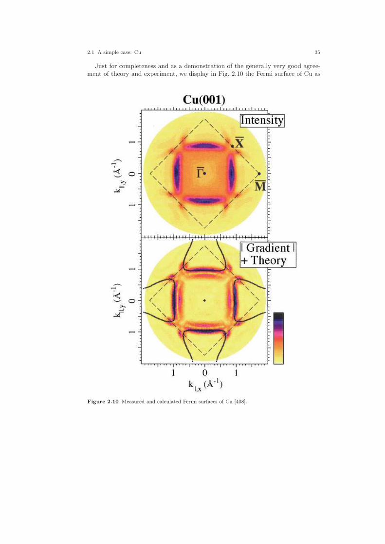
2.1 A simple case: Cu 35
Just for completeness and as a demonstration of the generally very good agree-ment of theory and experiment, we display in Fig. 2.10 the Fermi surface of Cu as
Figure 2.10 Measured and calculated Fermi surfaces of Cu [408].
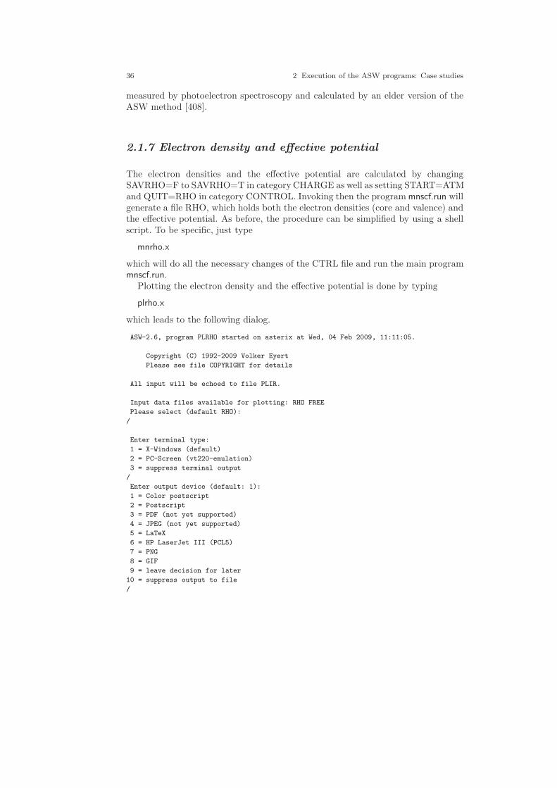
36 2 Execution of the ASW programs: Case studies
measured by photoelectron spectroscopy and calculated by an elder version of theASW method [408].
2.1.7 Electron density and effective potential
The electron densities and the effective potential are calculated by changingSAVRHO=F to SAVRHO=T in category CHARGE as well as setting START=ATMand QUIT=RHO in category CONTROL. Invoking then the program mnscf.run willgenerate a file RHO, which holds both the electron densities (core and valence) andthe effective potential. As before, the procedure can be simplified by using a shellscript. To be specific, just type
mnrho.x
which will do all the necessary changes of the CTRL file and run the main programmnscf.run.
Plotting the electron density and the effective potential is done by typing
plrho.x
which leads to the following dialog.
ASW-2.6, program PLRHO started on asterix at Wed, 04 Feb 2009, 11:11:05.
Copyright (C) 1992-2009 Volker Eyert
Please see file COPYRIGHT for details
All input will be echoed to file PLIR.
Input data files available for plotting: RHO FREE
Please select (default RHO):
/
Enter terminal type:
1 = X-Windows (default)
2 = PC-Screen (vt220-emulation)
3 = suppress terminal output
/
Enter output device (default: 1):
1 = Color postscript
2 = Postscript
3 = PDF (not yet supported)
4 = JPEG (not yet supported)
5 = LaTeX
6 = HP LaserJet III (PCL5)
7 = PNG
8 = GIF
9 = leave decision for later
10 = suppress output to file
/
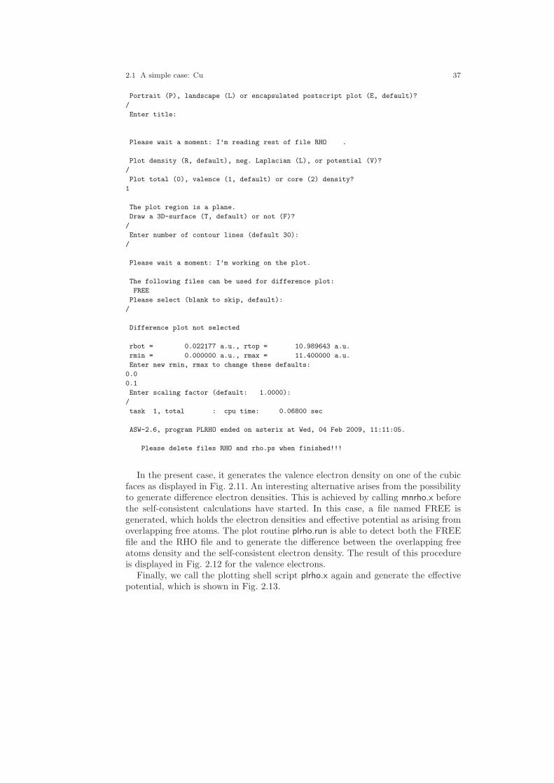
2.1 A simple case: Cu 37
Portrait (P), landscape (L) or encapsulated postscript plot (E, default)?
/
Enter title:
Please wait a moment: I’m reading rest of file RHO .
Plot density (R, default), neg. Laplacian (L), or potential (V)?
/
Plot total (0), valence (1, default) or core (2) density?
1
The plot region is a plane.
Draw a 3D-surface (T, default) or not (F)?
/
Enter number of contour lines (default 30):
/
Please wait a moment: I’m working on the plot.
The following files can be used for difference plot:
FREE
Please select (blank to skip, default):
/
Difference plot not selected
rbot = 0.022177 a.u., rtop = 10.989643 a.u.
rmin = 0.000000 a.u., rmax = 11.400000 a.u.
Enter new rmin, rmax to change these defaults:
0.0
0.1
Enter scaling factor (default: 1.0000):
/
task 1, total : cpu time: 0.06800 sec
ASW-2.6, program PLRHO ended on asterix at Wed, 04 Feb 2009, 11:11:05.
Please delete files RHO and rho.ps when finished!!!
In the present case, it generates the valence electron density on one of the cubicfaces as displayed in Fig. 2.11. An interesting alternative arises from the possibilityto generate difference electron densities. This is achieved by calling mnrho.x beforethe self-consistent calculations have started. In this case, a file named FREE isgenerated, which holds the electron densities and effective potential as arising fromoverlapping free atoms. The plot routine plrho.run is able to detect both the FREEfile and the RHO file and to generate the difference between the overlapping freeatoms density and the self-consistent electron density. The result of this procedureis displayed in Fig. 2.12 for the valence electrons.
Finally, we call the plotting shell script plrho.x again and generate the effectivepotential, which is shown in Fig. 2.13.

38 2 Execution of the ASW programs: Case studies
0 10 20 30 40 50 0 10
20 30
40 50
0.02 0.03 0.04 0.05 0.06 0.07 0.08 0.09 0.1
0.11
ρv / a.u.
Figure 2.11 Valence electron density of Cu.
0 10 20 30 40 50 0 10
20 30
40 50
-0.06-0.04-0.02
0 0.02 0.04 0.06 0.08
ρv / a.u.
Figure 2.12 Valence electron density difference of Cu.
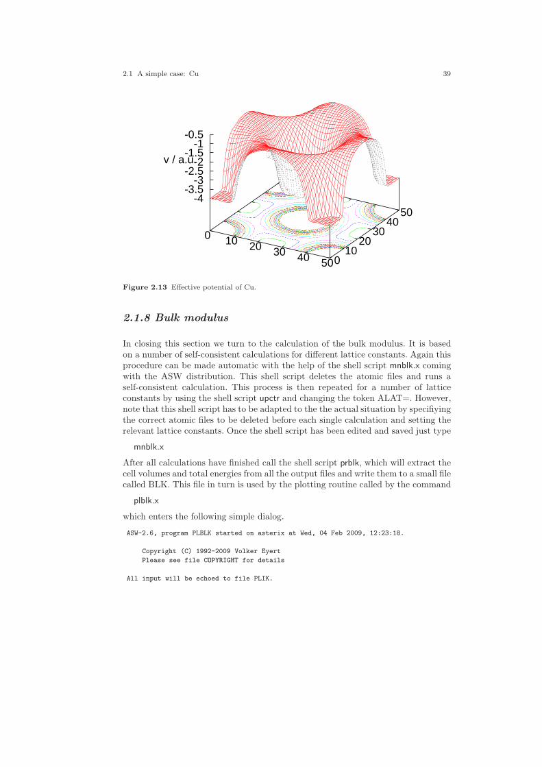
2.1 A simple case: Cu 39
0 10 20 30 40 50 0 10
20 30
40 50
-4-3.5
-3-2.5
-2-1.5
-1-0.5
v / a.u.
Figure 2.13 Effective potential of Cu.
2.1.8 Bulk modulus
In closing this section we turn to the calculation of the bulk modulus. It is basedon a number of self-consistent calculations for different lattice constants. Again thisprocedure can be made automatic with the help of the shell script mnblk.x comingwith the ASW distribution. This shell script deletes the atomic files and runs aself-consistent calculation. This process is then repeated for a number of latticeconstants by using the shell script upctr and changing the token ALAT=. However,note that this shell script has to be adapted to the the actual situation by specifiyingthe correct atomic files to be deleted before each single calculation and setting therelevant lattice constants. Once the shell script has been edited and saved just type
mnblk.x
After all calculations have finished call the shell script prblk, which will extract thecell volumes and total energies from all the output files and write them to a small filecalled BLK. This file in turn is used by the plotting routine called by the command
plblk.x
which enters the following simple dialog.
ASW-2.6, program PLBLK started on asterix at Wed, 04 Feb 2009, 12:23:18.
Copyright (C) 1992-2009 Volker Eyert
Please see file COPYRIGHT for details
All input will be echoed to file PLIK.
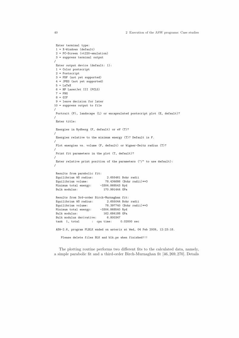
40 2 Execution of the ASW programs: Case studies
Enter terminal type:
1 = X-Windows (default)
2 = PC-Screen (vt220-emulation)
3 = suppress terminal output
/
Enter output device (default: 1):
1 = Color postscript
2 = Postscript
3 = PDF (not yet supported)
4 = JPEG (not yet supported)
5 = LaTeX
6 = HP LaserJet III (PCL5)
7 = PNG
8 = GIF
9 = leave decision for later
10 = suppress output to file
/
Portrait (P), landscape (L) or encapsulated postscript plot (E, default)?
/
Enter title:
Energies in Rydberg (F, default) or eV (T)?
/
Energies relative to the minimum energy (T)? Default is F.
/
Plot energies vs. volume (F, default) or Wigner-Seitz radius (T)?
/
Print fit parameters in the plot (T, default)?
/
Enter relative print position of the parameters ("/" to use default):
/
Results from parabolic fit:
Equilibrium WS radius: 2.655461 Bohr radii
Equilibrium volume: 78.434686 (Bohr radii)**3
Minimum total energy: -3304.868543 Ryd
Bulk modulus: 170.991444 GPa
Results from 3rd-order Birch-Murnaghan fit:
Equilibrium WS radius: 2.655044 Bohr radii
Equilibrium volume: 78.397740 (Bohr radii)**3
Minimum total energy: -3304.868540 Ryd
Bulk modulus: 162.684188 GPa
Bulk modulus derivative: 6.800347
task 1, total : cpu time: 0.02000 sec
ASW-2.6, program PLBLK ended on asterix at Wed, 04 Feb 2009, 12:23:18.
Please delete files BLK and blk.ps when finished!!!
The plotting routine performs two different fits to the calculated data, namely,a simple parabolic fit and a third-order Birch-Murnaghan fit [46, 269, 270]. Details

2.2 A semiconductor: Si 41
can also be found in my book [404]. The results of both fits are printed in the abovedialog. In addition, if this has been chosen, they are also displayed in the resultingplot, which is displayed in Fig. 2.14.
-3304.868600
-3304.868500
-3304.868400
-3304.868300
-3304.868200
-3304.868100
-3304.868000
-3304.867900
75.5 76 76.5 77 77.5 78 78.5 79 79.5 80 80.5
E (
Ryd
)
V (aB3)
V0 = 78.40 aB3
E0 = -3304.868540 Ryd
B0 = 162.68 GPa
Figure 2.14 Bulk modulus of Cu.
2.2 A semiconductor: Si
Another prominent test case for electronic structure methods and codes is elementalsilicon. As well known, silicon is a semiconductor with an indirect optical bandgapof about 1.1 eV, which crystallizes in the diamond structure shown in Fig. 2.15.Of course, interest in this material stems from its huge impact on semiconductorapplications during the last decades. Yet, being an elemental system it represents asufficiently simple test case.
The electronic structure of silicon is dominated by the 3s and 3p valence states,which also give the largest contributions at the valence band maximum and theconduction band minimum. As compared to the elemental metals, calculations forsilicon are confronted with two major challenges. First, the correct representation ofthe wave function, the electron density and the effective potential within the opendiamond crystal structure requires new means. This is due to the fact that suchopen structures can only be badly filled with the atomic spheres surrounding eachatom. Instead, rather large voids remain. However, the above quantities have to bealso well respresented within these voids. In a plane wave representation, this is doneby introducing a uniform mesh in the unit cell. In contrast, in a method based on
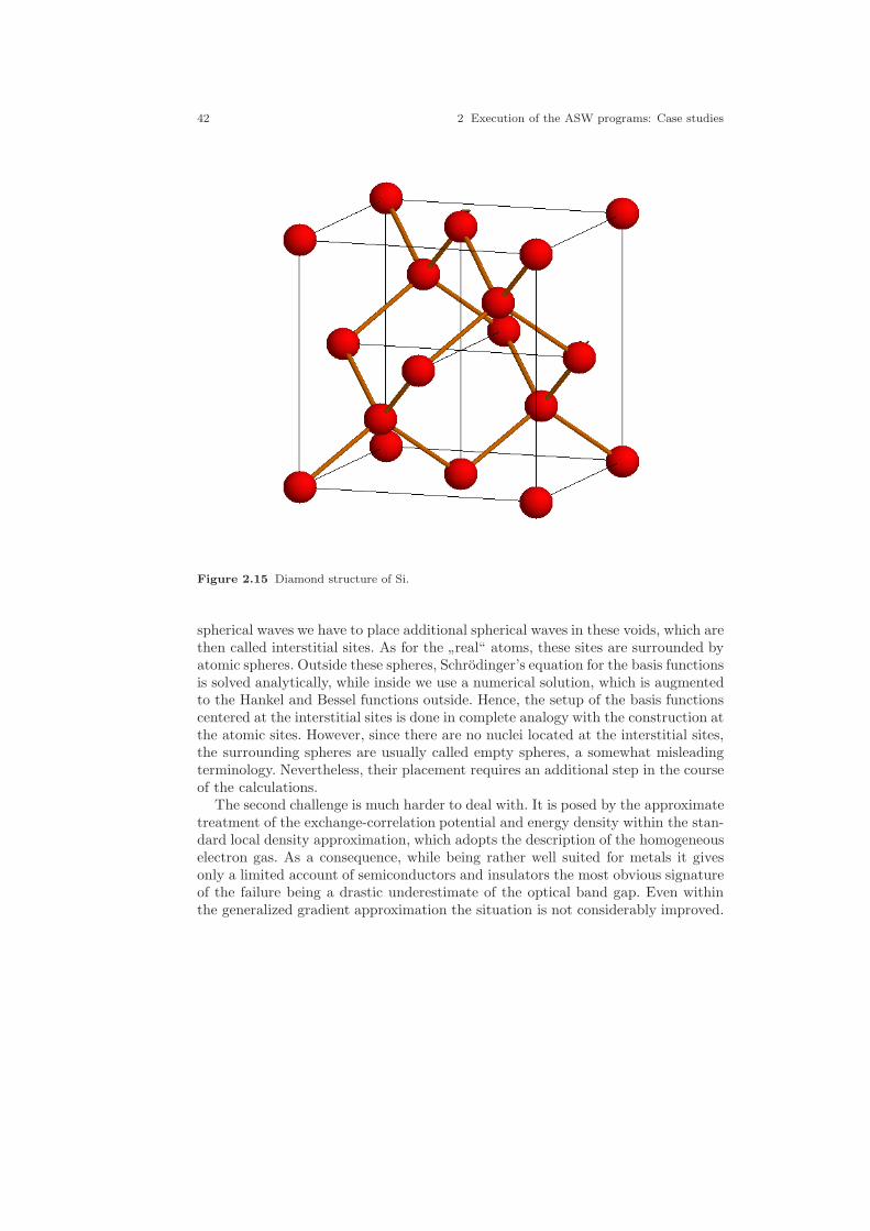
42 2 Execution of the ASW programs: Case studies
Figure 2.15 Diamond structure of Si.
spherical waves we have to place additional spherical waves in these voids, which arethen called interstitial sites. As for the
”real“ atoms, these sites are surrounded by
atomic spheres. Outside these spheres, Schrodinger’s equation for the basis functionsis solved analytically, while inside we use a numerical solution, which is augmentedto the Hankel and Bessel functions outside. Hence, the setup of the basis functionscentered at the interstitial sites is done in complete analogy with the construction atthe atomic sites. However, since there are no nuclei located at the interstitial sites,the surrounding spheres are usually called empty spheres, a somewhat misleadingterminology. Nevertheless, their placement requires an additional step in the courseof the calculations.
The second challenge is much harder to deal with. It is posed by the approximatetreatment of the exchange-correlation potential and energy density within the stan-dard local density approximation, which adopts the description of the homogeneouselectron gas. As a consequence, while being rather well suited for metals it givesonly a limited account of semiconductors and insulators the most obvious signatureof the failure being a drastic underestimate of the optical band gap. Even withinthe generalized gradient approximation the situation is not considerably improved.
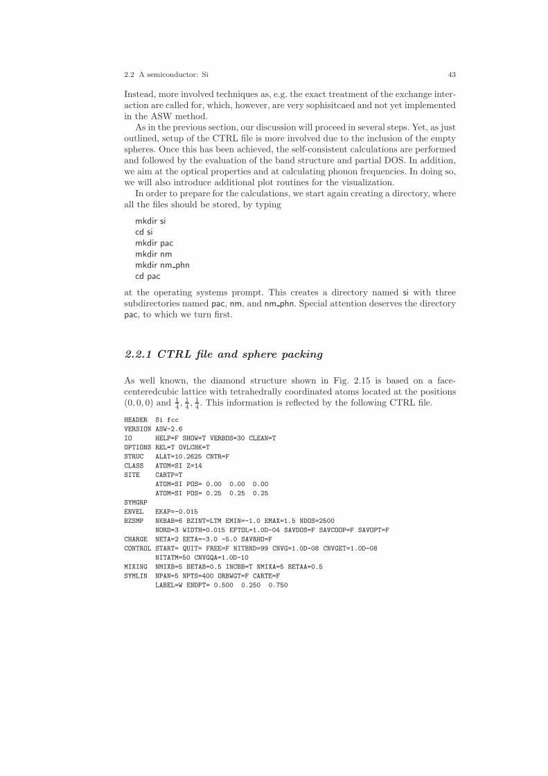
2.2 A semiconductor: Si 43
Instead, more involved techniques as, e.g. the exact treatment of the exchange inter-action are called for, which, however, are very sophisitcaed and not yet implementedin the ASW method.
As in the previous section, our discussion will proceed in several steps. Yet, as justoutlined, setup of the CTRL file is more involved due to the inclusion of the emptyspheres. Once this has been achieved, the self-consistent calculations are performedand followed by the evaluation of the band structure and partial DOS. In addition,we aim at the optical properties and at calculating phonon frequencies. In doing so,we will also introduce additional plot routines for the visualization.
In order to prepare for the calculations, we start again creating a directory, whereall the files should be stored, by typing
mkdir sicd simkdir pacmkdir nmmkdir nm phncd pac
at the operating systems prompt. This creates a directory named si with threesubdirectories named pac, nm, and nm phn. Special attention deserves the directorypac, to which we turn first.
2.2.1 CTRL file and sphere packing
As well known, the diamond structure shown in Fig. 2.15 is based on a face-centeredcubic lattice with tetrahedrally coordinated atoms located at the positions(0, 0, 0) and 1
4, 1
4, 1
4. This information is reflected by the following CTRL file.
HEADER Si fcc
VERSION ASW-2.6
IO HELP=F SHOW=T VERBOS=30 CLEAN=T
OPTIONS REL=T OVLCHK=T
STRUC ALAT=10.2625 CNTR=F
CLASS ATOM=SI Z=14
SITE CARTP=T
ATOM=SI POS= 0.00 0.00 0.00
ATOM=SI POS= 0.25 0.25 0.25
SYMGRP
ENVEL EKAP=-0.015
BZSMP NKBAB=6 BZINT=LTM EMIN=-1.0 EMAX=1.5 NDOS=2500
NORD=3 WIDTH=0.015 EFTOL=1.0D-04 SAVDOS=F SAVCOOP=F SAVOPT=F
CHARGE NETA=2 EETA=-3.0 -5.0 SAVRHO=F
CONTROL START= QUIT= FREE=F NITBND=99 CNVG=1.0D-08 CNVGET=1.0D-08
NITATM=50 CNVGQA=1.0D-10
MIXING NMIXB=5 BETAB=0.5 INCBB=T NMIXA=5 BETAA=0.5
SYMLIN NPAN=5 NPTS=400 ORBWGT=F CARTE=F
LABEL=W ENDPT= 0.500 0.250 0.750
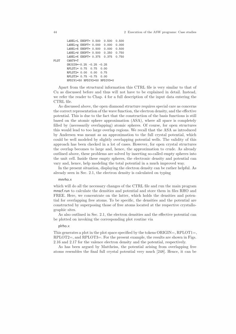
44 2 Execution of the ASW programs: Case studies
LABEL=L ENDPT= 0.500 0.500 0.500
LABEL=g ENDPT= 0.000 0.000 0.000
LABEL=X ENDPT= 0.500 0.000 0.500
LABEL=W ENDPT= 0.500 0.250 0.750
LABEL=K ENDPT= 0.375 0.375 0.750
PLOT CARTV=T
ORIGIN=-0.25 -0.25 -0.25
RPLOT1= 0.75 0.75 0.00
RPLOT2= 0.00 0.00 0.75
RPLOT3= 0.75 -0.75 0.00
NPDIV1=50 NPDIV2=50 NPDIV3=0
Apart from the structural information this CTRL file is very similar to that ofCu as discussed before and thus will not have to be explained in detail. Instead,we refer the reader to Chap. 4 for a full description of the input data entering theCTRL file.
As discussed above, the open diamond structure requires special care as concernsthe correct representation of the wave function, the electron density, and the effectivepotential. This is due to the fact that the construction of the basis functions is stillbased on the atomic sphere approximation (ASA), where all space is completelyfilled by (necessarily overlapping) atomic spheres. Of course, for open structuresthis would lead to too large overlap regions. We recall that the ASA as introducedby Andersen was meant as an approximation to the full crystal potential, whichcould be well modeled by slightly overlapping potential wells. The validity of thisapproach has been checked in a lot of cases. However, for open crystal structuresthe overlap becomes to large and, hence, the approximation to crude. As alreadyoutlined above, these problems are solved by inserting so-called empty spheres intothe unit cell. Inside these empty spheres, the electronic density and potential canvary and, hence, help modeling the total potential in a much improved way.
In the present situation, displaying the electron density can be rather helpful. Asalready seen in Sec. 2.1, the electron density is calculated on typing
mnrho.x
which will do all the necessary changes of the CTRL file and run the main programmnscf.run to calculate the densities and potential and store them in files RHO andFREE. Here, we concentrate on the latter, which holds the densities and poten-tial for overlapping free atoms. To be specific, the densities and the potential areconstructed by superposing those of free atoms located at the respective crystallo-graphic sites.
As also outlined in Sec. 2.1, the electron densities and the effective potential canbe plotted on invoking the corresponding plot routine via
plrho.x
This generates a plot in the plot space specified by the tokens ORIGIN=, RPLOT1=,RPLOT2=, and RPLOT3=. For the present example, the results are shown in Figs.2.16 and 2.17 for the valence electron density and the potential, respectively.
As has been argued by Mattheiss, the potential arising from overlapping freeatoms resembles the final full crystal potential very much [248]. Hence, it can be
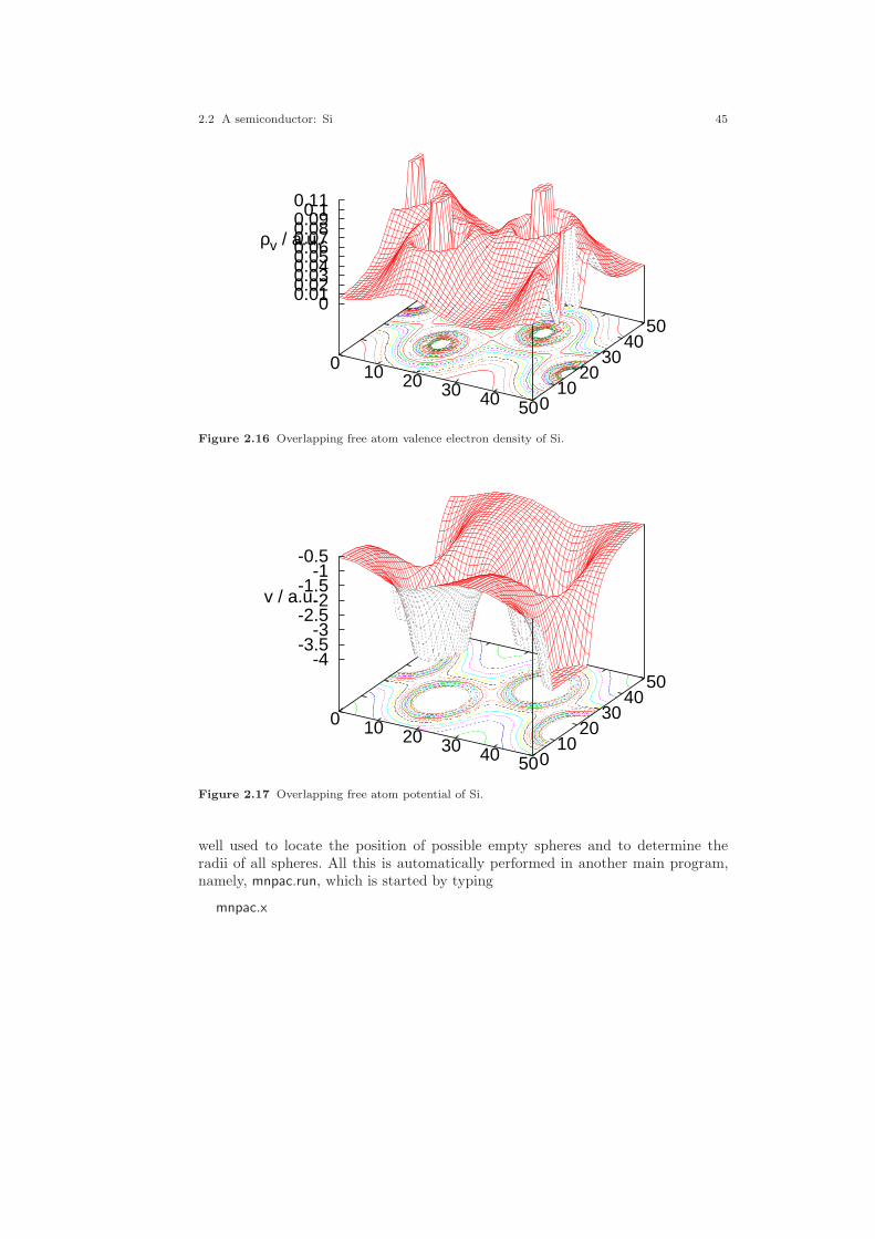
2.2 A semiconductor: Si 45
0 10 20 30 40 50 0 10
20 30
40 50
0 0.01 0.02 0.03 0.04 0.05 0.06 0.07 0.08 0.09 0.1 0.11
ρv / a.u.
Figure 2.16 Overlapping free atom valence electron density of Si.
0 10 20 30 40 50 0 10
20 30
40 50
-4-3.5
-3-2.5
-2-1.5
-1-0.5
v / a.u.
Figure 2.17 Overlapping free atom potential of Si.
well used to locate the position of possible empty spheres and to determine theradii of all spheres. All this is automatically performed in another main program,namely, mnpac.run, which is started by typing
mnpac.x

46 2 Execution of the ASW programs: Case studies
at the systems prompt. This routine runs the so-called sphere geometry optimization(SGO) algorithm, which consists of several steps. At the very beginning, it scans theoverlapping free atom potential along lines connecting the atoms and finds optimalmuffin-tin radii, i.e. radii for non-overlapping spheres. These are taken as a guidlinefor the atomic sphere radii. After that, it starts a search through the unit cell andidentifies that position, where the largest possible empty sphere could be placed.Actually, this is done by a genetic algorithm, which is a highly sophisticated methodfor multi-dimensional optimization [133]. Having found such an empty sphere candi-date, the radii of all spheres, including the “physical” spheres and all empty spheresfound so far, are blown up until an acceptable overlap is reached. With the resultingatomic sphere radii the overall space filling is checked, and if this is not yet com-plete, the process is repeated by searching for addtional empty spheres until theASA condition is obeyed.
After having performed all these steps, the program mnpac.run writes a newversion of the CTRL file to file CNEW, which contains all the empty sphere positionsas well as atomic sphere radii of all atoms. Recall that the programs never write tofile CTRL! Finally, mnpac.run proposes the number of partial waves for the emptyspheres. They are included by the tokens LMXL= and CONF=. Of course, thecorresponding charges as given by token QVAL= are all zero. The file CNEW looksas follows.
HEADER Si fcc
VERSION ASW-2.6
IO HELP=F SHOW=T VERBOS=30 CLEAN=T
OPTIONS REL=T OVLCHK=T
STRUC ALAT=10.2625 CNTR=F
CLASS ATOM=SI Z=14 R=2.47161370 LMXL=2 CONF=3 3 3 4
QVAL= 2.0 2.0 0.0 0.0
ATOM=E1 Z= 0 R=2.57907386 LMXL=2 CONF=1 2 3 4
QVAL= 0.0 0.0 0.0 0.0
SITE CARTP=T
ATOM=SI POS= 0.00 0.00 0.00
ATOM=SI POS= 0.25 0.25 0.25
ATOM=E1 POS=-0.25 -0.25 -0.25
ATOM=E1 POS= 0.00 0.00 0.50
SYMGRP
ENVEL EKAP=-0.015
BZSMP NKBAB=6 BZINT=LTM EMIN=-1.0 EMAX=1.5 NDOS=2500
NORD=3 WIDTH=0.015 SAVDOS=F SAVCOOP=F SAVOPT=F
CHARGE NETA=2 EETA=-3.0 -5.0 SAVRHO=F
CONTROL START= QUIT= FREE=F NITBND=99 CNVG=1.0D-08 CNVGET=1.0D-08
NITATM=50 CNVGQA=1.0D-10
MIXING NMIXB=5 BETAB=0.5 INCBB=T NMIXA=5 BETAA=0.5
SYMLIN NPAN=5 NPTS=400 ORBWGT=F CARTE=F
LABEL=W ENDPT= 0.500 0.250 0.750
LABEL=L ENDPT= 0.500 0.500 0.500
LABEL=g ENDPT= 0.000 0.000 0.000
LABEL=X ENDPT= 0.500 0.000 0.500
LABEL=W ENDPT= 0.500 0.250 0.750
LABEL=K ENDPT= 0.375 0.375 0.750
PLOT CARTV=T
2.2 A semiconductor: Si 47
ORIGIN=-0.25 -0.25 -0.25
RPLOT1= 0.75 0.75 0.00
RPLOT2= 0.00 0.00 0.75
RPLOT3= 0.75 -0.75 0.00
NPDIV1=50 NPDIV2=50 NPDIV3=0
Obviously, two empty spheres have been added with radii slighty larger thanthose of the
”physical“ spheres. This is due to the fact that empty spheres are
allowed to have a slighty larger overlap than the”physical“ spheres as the potential
within these spheres is rather flat.All actions taken by the packing program mnpac.run are recorded in the output
file outpac, which among other things contains the results of a final overlap check forOVLCHK=T. There the overlap limits are repeated (as a default a linear overlapof 15% is used) and all lines with a linear overlap larger than 10% complementedby one or more exclamation marks. Note that an extra overlap bonus is given tothe empty spheres due to the flatness of the potential within these spheres.
2.2.2 Execution of the main programs
With the new CTRL file at hand we are able to perform the set of self-consistentcalculations. To this end we copy the CNEW file generated in the subdirectory pacto the CTRL file of subdirectory nm and start the calculations by typing
mnscf.x
or else
mnall.x
in case we want to all calculations in one go. After about two minutes the cal-culations have finished. A first impression of the outcome can be gained via thecommand
monic outlst18
which generates the following summary of the output file outlst18.
ASW-2.6, program MNSCF started on asterix at Wed, 04 Feb 2009, 15:49:59.
Calculation converged after 7 iteration(s).
Start of Iteration 7
220 irreducible k-points generated from 6859 ( 19, 19, 19).
Fermi energy - MTZ = 0.707668 Ryd.
The system is a semiconductor:
Indirect band gap = 0.040429 Ryd = 0.550058 eV
Mean-square residual: 0.122585D-23
Total free atom energies : -1155.304982 Ryd
Total variational energy : -1156.092086 Ryd
Cohesive energy : 0.787104 Ryd
qdiff = 0.00000000 < 0.00000001
ediff = 0.00000000 < 0.00000001

48 2 Execution of the ASW programs: Case studies
ASW-2.6, program MNSCF ended on asterix at Wed, 04 Feb 2009, 15:50:35.
According to this summary, silicon is correctly identified as a semiconductor withan indirect optical band gap. However, the band gap is by a factor of two to small,which, as mentioned above, is usual for calculations based on the local densityapproximation. The evaluation of the band gap results from a rather simple proce-dure. During the Brillouin zone scan the minimum and maximum energy of eachband are calculated together with the corresponding k-points. From this the size ofthe bandgap as well as valence band maximum and conduction band minimum forsemiconductors are calculated. Moreover, the Fermi energy is fixed to the midpointof the gap. Finally, all this information is written to the atomic files and to filesBNDE, DOS and COOP.
2.2.3 Execution of the plot programs
By now, we are in a position to invoke the plotting routines. As before, an image ofthe crystal structure is obtained by either typing
plxcr.x STRX
at the systems prompt and entering XCrysDen or else via
plstr.x
and going through the subsequent dialog, which leads to the visualization toolsRasMol.
ASW-2.6, program PLSTR started on asterix at Sun, 08 Feb 2009, 14:33:46.
Copyright (C) 1992-2009 Volker Eyert
Please see file COPYRIGHT for details
All input will be echoed to file PLIS.
Enter terminal type:
1 = X-Windows (default)
2 = PC-Screen (vt220-emulation)
3 = suppress terminal output
/
Enter output device (default: 1):
1 = Color postscript
2 = Postscript
3 = GIF
/
Enter title:
Use unit cell (F, default) or Wigner-Seitz cell (T)?
/
2.2 A semiconductor: Si 49
The following colours have been assigned to the classes:
SI : red ,
Select classes to be assigned a new colour
(enter blank or "/" when you’re done):
/
By default the bonds will be coloured orange .
Enter blank or "/" to accept or select from the following colours:
red [r ], green [g ], blue [b ], yellow [y ]
magenta [m ], cyan [c ], orange [o ], blueviolet [bv]
cyanogreen [cg], yellowgreen [yg], purple [p ], cyanoblue [cb]
violet [v ], pale red [pr], pale blue [pb], pale green [pg]
pale yellow [py], pale violet [pv], pale cyan [pc], black [bk]
gray1 (dark) [g1], gray2 [g2], gray3 [g3], gray4 [g4]
gray5 [g5], gray6 (lght) [g6], white [wh]
Muffin-tin spheres (M, default), ASA spheres (A), linear radii scaling (R)
or linear volume scaling (V):
R
Enter scale factor [ 0.100... 1.432] (default: 1.000):
0.6
The plot space contains 1 unit cell(s).
Enter strings for rotations. Default strings are:
rotate x 90
rotate y -5
rotate x 10
Overwrite or enter "/" when you’re done.
/
task 1, total : cpu time: 0.00800 sec
ASW-2.6, program PLSTR ended on asterix at Sun, 08 Feb 2009, 14:33:46.
Please delete files STRU and stru.* when finished!!!
Note that all your input to the plot routine plstr.run has been echoed to the filePLIS for repeated use.
Next the electronic band structure is plotted using the command
plbnd.x
and entering the following dialog. Note that for semiconductors and insulators theplotting routines plbnd.run, pldos.run, and plcop.run allow for different choices ofthe energy zero, which may be the muffin-tin zero, the Fermi energy, the valenceband maximum, or the conduction band minimum. The electronic band structureis displayed in Fig. 2.18. Here, a parabolic band starting at the Γ -point at about−12 eV and mainly resulting from the 3s orbitals is well recognized. In contrast, at

50 2 Execution of the ASW programs: Case studies
-12
-10
-8
-6
-4
-2
0
2
4
6
W L Γ X W K
(E -
EV)
(eV
)
Figure 2.18 Electronic structure of Si along selected symmetry lines of the first Brillouin zoneof the face-centered cubic lattice, see B.1.
the valence band maximum a threefold degenerate band is found, which traces backto the 3p states.
As before, the partial densities of states are obtained by typing
pldos.x
and follwoing the subsequent dialog. The result is displayed in Fig. 2.19, where weidentify the strong 3s and 3p contributions at the bottom and the top, respectively,of the valence band.
2.2.4 Electron density and effective potential
As described in Sec. 2.1, the electron densities and the effective potential are ob-tained by calling the shell script
mnrho.x
which does all the necessary changes of the CTRL file and runs the main programmnscf.run. Subsequently, the electron densities and the effective potential are disi-played by typing
plrho.x
and following the dialog. It generates the valence electron density as displayed inFig. 2.20. Comparing it to the valence electron density arising from overlapping free
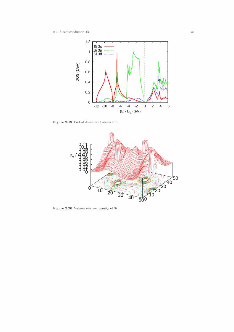
2.2 A semiconductor: Si 51
0
0.2
0.4
0.6
0.8
1
1.2
-12 -10 -8 -6 -4 -2 0 2 4 6
DO
S (
1/eV
)
(E - EV) (eV)
Si 3sSi 3pSi 3d
Figure 2.19 Partial densities of states of Si.
0 10 20 30 40 50 0 10
20 30
40 50
0 0.01 0.02 0.03 0.04 0.05 0.06 0.07 0.08 0.09 0.1 0.11
ρv / a.u.
Figure 2.20 Valence electron density of Si.

52 2 Execution of the ASW programs: Case studies
atoms as shown in Fig. 2.16 we recognize especially the double maxima betweenthe silicon atoms. They can be easily visualized by plotting the difference density,which is generated by calling mnrho.x twice, namely, once before the self-consistentset of calculations and once after completion of these calculations. The first step hasbeen already described above. It generated the file FREE, which stores the electrondensities and effective potential as arising from overlapping free atoms. In contrast,after the self-consistent calculations call of mnrho.x writes these quantities to fileRHO. The plot routine plrho.run will detect both the FREE file and the RHO fileand allows to generate the difference between the overlapping free atoms densityand the self-consistent electron density; just follow the dialog. The result of thisprocedure is displayed in Fig. 2.21 for the valence electrons. As mentioned above,
0 10 20 30 40 50 0 10
20 30
40 50
-0.06-0.04-0.02
0 0.02 0.04 0.06 0.08 0.1
0.12
ρv / a.u.
Figure 2.21 Valence electron density difference of Si.
we identifiy the pronounced double maxima between the atoms, which indicate theincreased covalent chemical bonding.
In order to visualize the chemical bonding, solid state chemists have introduceda variety of so-called bonding indicators. Among these are the electron localizationfunction and the negative Laplacian of the electron density. Evaluation of the latteris also implemented in the ASW programs and done along the calculation of theelectron density. Visualization is also provided by the plot routine plrho.x; the resultis shown in Fig. 2.22. Obviously, the negative Laplacian of the electron densitypronounces the fine details of the latter and thus is well suited to visualize covalentbonds.
Finally, we call the plotting shell script plrho.x again and generate the effectivepotential, which is shown in Fig. 2.23.
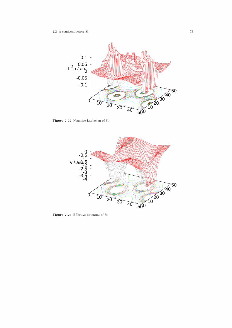
2.2 A semiconductor: Si 53
0 10 20 30 40 50 0 10
20 30
40 50
-0.1
-0.05
0
0.05
0.1
-∇ 2ρ / a.u.
Figure 2.22 Negative Laplacian of Si.
0 10 20 30 40 50 0 10
20 30
40 50
-4-3.5
-3-2.5
-2-1.5
-1-0.5
0
v / a.u.
Figure 2.23 Effective potential of Si.
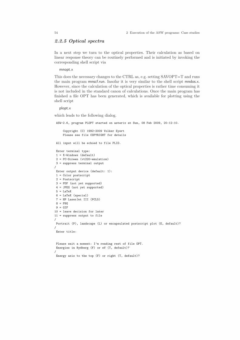
54 2 Execution of the ASW programs: Case studies
2.2.5 Optical spectra
In a next step we turn to the optical properties. Their calculation as based onlinear response theory can be routinely performed and is initiated by invoking thecorresponding shell script via
mnopt.x
This does the necessary changes to the CTRL as, e.g. setting SAVOPT=T and runsthe main program mnscf.run. Insofar it is very similar to the shell script mndos.x.However, since the calculation of the optical properties is rather time consuming itis not included in the standard canon of calculations. Once the main program hasfinished a file OPT has been generated, which is available for plotting using theshell script
plopt.x
which leads to the following dialog.
ASW-2.6, program PLOPT started on asterix at Sun, 08 Feb 2009, 20:12:10.
Copyright (C) 1992-2009 Volker Eyert
Please see file COPYRIGHT for details
All input will be echoed to file PLIO.
Enter terminal type:
1 = X-Windows (default)
2 = PC-Screen (vt220-emulation)
3 = suppress terminal output
/
Enter output device (default: 1):
1 = Color postscript
2 = Postscript
3 = PDF (not yet supported)
4 = JPEG (not yet supported)
5 = LaTeX
6 = LaTeX (special)
7 = HP LaserJet III (PCL5)
8 = PNG
9 = GIF
10 = leave decision for later
11 = suppress output to file
/
Portrait (P), landscape (L) or encapsulated postscript plot (E, default)?
/
Enter title:
Please wait a moment: I’m reading rest of file OPT.
Energies in Rydberg (F) or eV (T, default)?
/
Energy axis to the top (F) or right (T, default)?

2.2 A semiconductor: Si 55
/
Plot OPT (F, default) or integrated OPT (T)?
/
Start setting up curve 1:
Select Cartesian components of the tensor (default xx).
/
Plot optical conductivity (SIG, default), dielectric function (EPS),
refraction index (RFI), optical reflectivity (REF),
optical absorption (ABS), electron loss function (ELF)?
/
Plot absorptive (A, default) or dispersive part (D)?
/
Plot real (R, default) or imaginary part (I)?
/
Select from the occ bands of the OPT matrix:
Plot selected (F) or all occ bands (T, default)?
/
Select from the unocc bands of the OPT matrix:
Plot selected (F) or all unocc bands (T, default)?
/
Include intraband contributions (T) or not (F, default)?
/
Multiply with energy (F, default)?
/
Broadening of this curve (T) or not (F, default)?
/
Select curve style (default: 1) (A * marks styles already selected):
solid/green (1) , dash1/blue (2) ,
dash2/red (3) , dot/magenta (4) ,
dashdot1/cyan (5) , dashdot2/yellow (6) ,
chaindash1/black (7) , chaindash2/coral (8) ,
chaindash3/gray (9) ,
/
Enter curve label ("/" to suppress)
Re {/Symbol s}_{a, xx}
Please wait a moment: I’m working on this curve.
Set up more curves (T)? Default is F.
T
Start setting up curve 2:
Select Cartesian components of the tensor (default xx).
/
Plot optical conductivity (SIG, default), dielectric function (EPS),
refraction index (RFI), optical reflectivity (REF),
optical absorption (ABS), electron loss function (ELF)?
/
Plot absorptive (A, default) or dispersive part (D)?
D
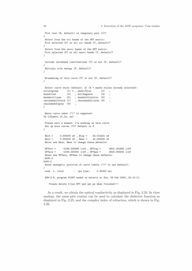
56 2 Execution of the ASW programs: Case studies
Plot real (R, default) or imaginary part (I)?
I
Select from the occ bands of the OPT matrix:
Plot selected (F) or all occ bands (T, default)?
/
Select from the unocc bands of the OPT matrix:
Plot selected (F) or all unocc bands (T, default)?
/
Include intraband contributions (T) or not (F, default)?
/
Multiply with energy (F, default)?
/
Broadening of this curve (T) or not (F, default)?
/
Select curve style (default: 2) (A * marks styles already selected):
solid/green (1) * , dash1/blue (2) ,
dash2/red (3) , dot/magenta (4) ,
dashdot1/cyan (5) , dashdot2/yellow (6) ,
chaindash1/black (7) , chaindash2/coral (8) ,
chaindash3/gray (9) ,
/
Enter curve label ("/" to suppress)
Im {/Symbol s}_{a, xx}
Please wait a moment: I’m working on this curve.
Set up more curves (T)? Default is F.
/
Ebot = 0.000000 eV , Etop = 34.014231 eV
Emin = 0.000000 eV , Emax = 35.000000 eV
Enter new Emin, Emax to change these defaults:
OPTbot = -2158.229369 1/eV , OPTtop = 4815.191685 1/eV
OPTmin = -2160.000000 1/eV , OPTmax = 4820.000000 1/eV
Enter new OPTmin, OPTmax to change these defaults:
-2500.0
5000.0
Enter energetic position of curve labels ("/" to use default):
/
task 1, total : cpu time: 0.45203 sec
ASW-2.6, program PLOPT ended on asterix at Sun, 08 Feb 2009, 20:12:11.
Please delete files OPT and opt.ps when finished!!!
As a result, we obtain the optical conductivity as displayed in Fig. 2.24. In closeanalogy, the same plot routine can be used to calculate the dielectric function asdisplayed in Fig. 2.25, and the complex index of refraction, which is shown in Fig.2.26.
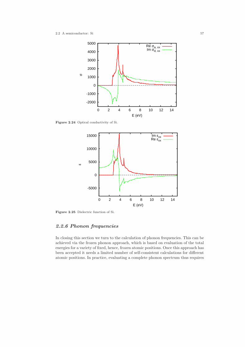
2.2 A semiconductor: Si 57
-2000
-1000
0
1000
2000
3000
4000
5000
0 2 4 6 8 10 12 14
σ
E (eV)
Re σa, xxIm σd, xx
Figure 2.24 Optical conductivity of Si.
-5000
0
5000
10000
15000
0 2 4 6 8 10 12 14
ε
E (eV)
Im εxxRe εxx
Figure 2.25 Dielectric function of Si.
2.2.6 Phonon frequencies
In closing this section we turn to the calculation of phonon frequencies. This can beachieved via the frozen phonon approach, which is based on evaluation of the totalenergies for a variety of fixed, hence, frozen atomic positions. Once this approach hasbeen accepted it needs a limited number of self-consistent calculations for differentatomic positions. In practice, evaluating a complete phonon spectrum thus requires
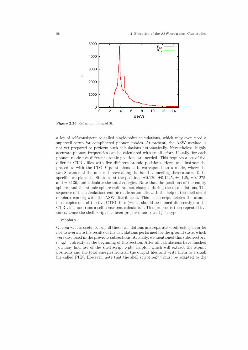
58 2 Execution of the ASW programs: Case studies
0
1000
2000
3000
4000
5000
0 2 4 6 8 10 12 14
σ
E (eV)
nxxkxx
Figure 2.26 Refraction index of Si.
a lot of self-consistent so-called single-point calculations, which may even need asupercell setup for complicated phonon modes. At present, the ASW method isnot yet prepared to perform such calculations automatically. Nevertheless, highlyaccurate phonon frequencies can be calculated with small effort. Usually, for eachphonon mode five different atomic positions are needed. This requires a set of fivedifferent CTRL files with five different atomic positions. Here, we illustrate theprocedure with the LTO Γ -point phonon. It corresponds to a mode, where thetwo Si atoms of the unit cell move along the bond connecting these atoms. To bespecific, we place the Si atoms at the positions ±0.120, ±0.1225, ±0.125, ±0.1275,and ±0.130, and calculate the total energies. Note that the positions of the emptyspheres and the atomic sphere radii are not changed during these calculations. Thesequence of the calculations can be made automatic with the help of the shell scriptmnphn.x coming with the ASW distribution. This shell script deletes the atomicfiles, copies one of the five CTRL files (which should be named differently) to theCTRL file, and runs a self-consistent calculation. This process is then repeated fivetimes. Once the shell script has been prepared and saved just type
mnphn.x
Of course, it is useful to run all these calculations in a separate subdirectory in ordernot to overwrite the results of the calculations performed for the ground state, whichwere discussed in the previous subsections. Actually, we mentioned this subdirectory,nm phn, already at the beginning of this section. After all calculations have finishedyou may find use of the shell script prphn helpful, which will extract the atomicpositions and the total energies from all the output files and write them to a smallfile called PHN. However, note that the shell script prphn must be adapted to the

2.2 A semiconductor: Si 59
particular situation. Finally, the file PHN is used by the plotting routine called bythe command
plphn.x
which enters the following simple dialog.
ASW-2.6, program PLPHN started on asterix at Sun, 08 Feb 2009, 14:37:47.
Copyright (C) 1992-2009 Volker Eyert
Please see file COPYRIGHT for details
All input will be echoed to file PLIP.
Enter terminal type:
1 = X-Windows (default)
2 = PC-Screen (vt220-emulation)
3 = suppress terminal output
/
Enter output device (default: 1):
1 = Color postscript
2 = Postscript
3 = PDF (not yet supported)
4 = JPEG (not yet supported)
5 = LaTeX
6 = LaTeX (special)
7 = HP LaserJet III (PCL5)
8 = PNG
9 = GIF
10 = leave decision for later
11 = suppress output to file
/
Portrait (P), landscape (L) or encapsulated postscript plot (E, default)?
/
Enter title:
Energies in Rydberg (F, default) or eV (T)?
/
Energies relative to the minimum energy (T)? Default is F.
/
Print fit parameters in the plot (T, default)?
/
Enter relative print position of the parameters ("/" to use default):
/
Results from polynomial fit:
Equilibrium position: 0.125000
Minimum total energy: -1156.092085 Ryd
Force constant: 356.953174 Ryd/u**2
Cubic force constant: -4181.125308 Ryd/u**3
task 1, total : cpu time: 0.01600 sec
ASW-2.6, program PLPHN ended on asterix at Sun, 08 Feb 2009, 14:37:47.
Please delete files PHN and phn.ps when finished!!!

60 2 Execution of the ASW programs: Case studies
The plotting routine performs a 3rd-order polynomial fit to the calculated data.The result of this fit is printed in the above dialog. In addition, if this has beenchosen, the fit parameters are also displayed in the resulting plot, which is displayedin Fig. 2.27. Obviously, a stable minimum at the equilibrium position u0 = 0.125
-1156.093000
-1156.092000
-1156.091000
-1156.090000
-1156.089000
-1156.088000
-1156.087000
-1156.086000
0.118 0.12 0.122 0.124 0.126 0.128 0.13 0.132
E (
Ryd
)
u
u0 = 0.125000
E0 = -1156.092085 Ryd
k0 = 356.95 Ryd/u2
a0 = -4181.13 Ryd/u3
Figure 2.27 Total energy vs. Si position.
is obtained. This is a success of the full-potential treatment coming with the newASW method. For comparison we display in Fig. 2.28. the corresponding resultobtained from version 2.2, which is still based on the atomic sphere approximationbut already includes the nonspherical contributions to the electron densities andthe effective potential, hence, the abbreviation ASA+. The difference between bothcurves is striking and needs no further comments.
Still, we want to evaluate the force constant and the cubic force constant given inthe above dialog and in Fig. 2.27. To this end we first have to convert the differentvalues of u to A. Since the mode moves two atoms along the diagonal of the cubeand with a lattice constant of 10.2625aB, we obtain
k0 = 356.9532Ryd
u2= 2.0172
Ryd
A2
= 439.7262J
m2.
Combining this with the mass of one Si atom of M = 28.0855×1.6726231×10−27kgwe arrive at
k0
M= 9.3606× 1027s−2 ,
which leads to
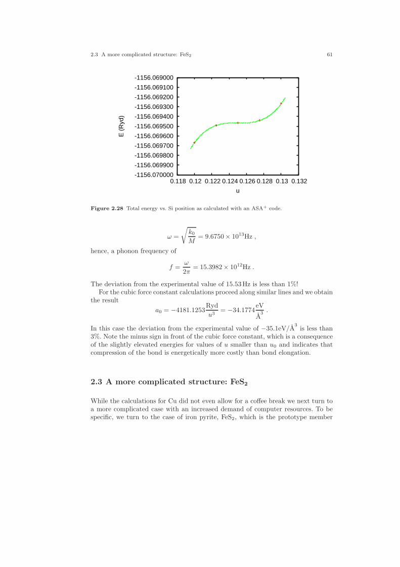
2.3 A more complicated structure: FeS2 61
-1156.070000
-1156.069900
-1156.069800
-1156.069700
-1156.069600
-1156.069500
-1156.069400
-1156.069300
-1156.069200
-1156.069100
-1156.069000
0.118 0.12 0.122 0.124 0.126 0.128 0.13 0.132
E (
Ryd
)
u
Figure 2.28 Total energy vs. Si position as calculated with an ASA+ code.
ω =
√
k0
M= 9.6750× 10¹³Hz ,
hence, a phonon frequency of
f =ω
2π= 15.3982× 10¹²Hz .
The deviation from the experimental value of 15.53Hz is less than 1%!For the cubic force constant calculations proceed along similar lines and we obtain
the result
a0 = −4181.1253Ryd
u3= −34.1774
eV
A3.
In this case the deviation from the experimental value of −35.1eV/A3
is less than3%. Note the minus sign in front of the cubic force constant, which is a consequenceof the slightly elevated energies for values of u smaller than u0 and indicates thatcompression of the bond is energetically more costly than bond elongation.
2.3 A more complicated structure: FeS2
While the calculations for Cu did not even allow for a coffee break we next turn toa more complicated case with an increased demand of computer resources. To bespecific, we turn to the case of iron pyrite, FeS2, which is the prototype member
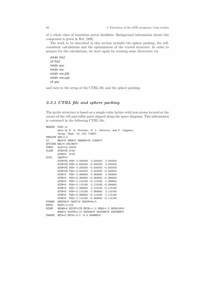
62 2 Execution of the ASW programs: Case studies
of a whole class of transition metal disulfides. Background information about thiscompound is given in Ref. [409].
The work to be described in this section includes the sphere packing, the self-consistent calculations and the optimization of the crystal structure. In order toprepare for the calculations, we start again by creating some directories via
mkdir fes2cd fes2mkdir pacmkdir nmmkdir nm blkmkdir nm optcd pac
and turn to the setup of the CTRL file and the sphere packing.
2.3.1 CTRL file and sphere packing
The pyrite structure is based on a simple cubic lattice with iron atoms located at thecorner of the cell and sulfur pairs aligned along the space diagonal. This informationis contained in the following CTRL file.
HEADER FeS2 sc
data by E. D. Stevens, M. L. DeLucia, and P. Coppens,
Inorg. Chem. 19, 813 (1980).
VERSION ASW-2.6
IO HELP=F SHOW=T VERBOS=30 CLEAN=T
OPTIONS REL=T OVLCHK=T
STRUC ALAT=10.23476
CLASS ATOM=FE Z=26
ATOM=S Z=16
SITE CARTP=T
ATOM=FE POS= 0.000000 0.000000 0.000000
ATOM=FE POS=-0.500000 -0.500000 0.000000
ATOM=FE POS= 0.000000 -0.500000 -0.500000
ATOM=FE POS=-0.500000 0.000000 -0.500000
ATOM=S POS= 0.384840 0.384840 0.384840
ATOM=S POS=-0.384840 -0.384840 -0.384840
ATOM=S POS= 0.115160 -0.115160 0.384840
ATOM=S POS=-0.115160 0.115160 -0.384840
ATOM=S POS= 0.384840 0.115160 -0.115160
ATOM=S POS=-0.115160 0.384840 0.115160
ATOM=S POS=-0.384840 -0.115160 0.115160
ATOM=S POS= 0.115160 -0.384840 -0.115160
SYMGRP GENPOS=F CARTT=F SGSYM=Pa-3
ENVEL EKAP=-0.015
BZSMP NKBAB=6 BZINT=LTM EMIN=-1.0 EMAX=1.5 NDOS=2500
NORD=3 WIDTH=0.01 SAVDOS=F SAVCOOP=F SAVFERM=F
CHARGE NETA=2 EETA=-3.0 -5.0 SAVRHO=F

2.3 A more complicated structure: FeS2 63
CONTROL START= QUIT= FREE=F NITBND=99 CNVG=1.0D-08 CNVGET=1.0D-08
NITATM=50 CNVGQA=1.0D-10
MIXING NMIXB=5 BETAB=0.5 INCBB=T NMIXA=5 BETAA=0.5
PLOT CARTV=T
ORIGIN= 0.5 0.0 0.0
RPLOT1= 1.0 0.0 0.0
RPLOT2= 0.0 1.0 0.0
RPLOT3= 0.0 0.0 1.0
NPDIV1=50 NPDIV2=50 NPDIV3=0
Due to the symmetry of the crystal the simple cubic cell comprises four iron andeight sulfur atoms in total. The crystal structure is shown in Fig. 2.29. In this plot
Figure 2.29 Crystal structure of FeS2. Iron and sulfur atoms are printed in red and yellow,respectively.
the origin has been shifted by half the cell edge (see token ORIGIN=0.5 0.0 0.0 incategory PLOT). As a consequence, one Fe atom is observed in the center of theplot while atoms of the sulfur pair appear in the upper right and lower left corner.
The pyrite crystal structure is best described in terms of the NaCl structurewith the sublattices occupied by iron atoms and the centers of gravity of sulfuratom pairs, respectively. These sulfur dumb-bells are oriented along the 〈111〉 axes.Being 2.161 A their bond length is still shorter than the Fe-S distance of 2.265 A.Whereas the sulfur atoms are tetrahedrally coordinated by one sulfur and three ironatoms the six nearest neighbour sulfur atoms at each iron site form slightly distorted

64 2 Execution of the ASW programs: Case studies
octahedra. The distorted FeS6 octahedra are interlinked by common corners and,due to the formation of the 〈111〉 sulfur pairs, have rotated away from the Cartesianaxes by about 23◦. For a two dimensional crystal the situation is sketched in Fig.2.30. Obviously, the formation of the 〈111〉 sulfur pairs does not destroy the square
~~ ~~ ~j j jj���
@@R���@@R�� @@I ��
@@Izz z zzz
z zJJJJJJJJJJJJ������������JJJJJJJJJJJJ������������
Figure 2.30 Two-dimensional analogue of the pyrite structure. Big and small filled circles desig-nate iron and sulfur atoms, respectively. Small open circles mark the ideal positions of the rocksaltstructure.
planar coordination of the iron atoms. Instead, the squares built by the sulfur atomsjust shrink and rotate. Since the orientation of the dumb-bells conforms with thecubic point group the underlying Bravais lattice is no longer face-centered but simplecubic and the unit cell comprises four formula units.
In the CTRL file listed above we have already included information aboutthe crystal symmetry in category SYMGRP. It contains three tokens, namely,SGSYM=, which specifies the space group of the pyrite structure. A full list ofall space groups and the coding of the space group symbols is given in the file SPC-GRP coming with the distribution. Alternatively, this file can be generated usingthe setting HELP=T and running any of the main programs. Instead of the tokenSGSYM= the token SYMOPS= could be used. With this token, a minimal set ofsymmetry operation, the socalled generators of the space group, can be specified.The generators are also given in the SPCGRP file. By building all products of thesegenerators the whole space group can be obtained.
The space group information can be used in two different ways. First, for GEN-POS=F the program performs a symmetry check using the information about thelattice and the atomic sites. As a result, the full space group information includinga list of all allowed symmetry operations is displayed. In addition, this information
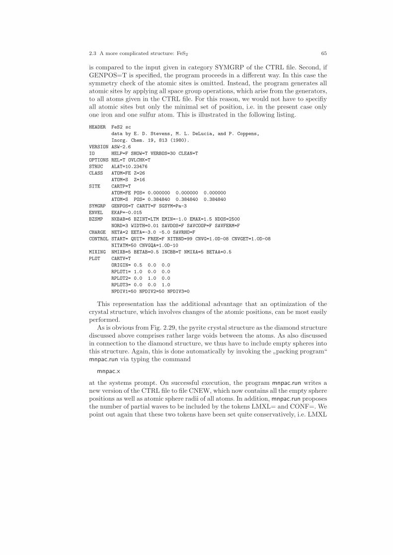
2.3 A more complicated structure: FeS2 65
is compared to the input given in category SYMGRP of the CTRL file. Second, ifGENPOS=T is specified, the program proceeds in a different way. In this case thesymmetry check of the atomic sites is omitted. Instead, the program generates allatomic sites by applying all space group operations, which arise from the generators,to all atoms given in the CTRL file. For this reason, we would not have to specifiyall atomic sites but only the minimal set of position, i.e. in the present case onlyone iron and one sulfur atom. This is illustrated in the following listing.
HEADER FeS2 sc
data by E. D. Stevens, M. L. DeLucia, and P. Coppens,
Inorg. Chem. 19, 813 (1980).
VERSION ASW-2.6
IO HELP=F SHOW=T VERBOS=30 CLEAN=T
OPTIONS REL=T OVLCHK=T
STRUC ALAT=10.23476
CLASS ATOM=FE Z=26
ATOM=S Z=16
SITE CARTP=T
ATOM=FE POS= 0.000000 0.000000 0.000000
ATOM=S POS= 0.384840 0.384840 0.384840
SYMGRP GENPOS=T CARTT=F SGSYM=Pa-3
ENVEL EKAP=-0.015
BZSMP NKBAB=6 BZINT=LTM EMIN=-1.0 EMAX=1.5 NDOS=2500
NORD=3 WIDTH=0.01 SAVDOS=F SAVCOOP=F SAVFERM=F
CHARGE NETA=2 EETA=-3.0 -5.0 SAVRHO=F
CONTROL START= QUIT= FREE=F NITBND=99 CNVG=1.0D-08 CNVGET=1.0D-08
NITATM=50 CNVGQA=1.0D-10
MIXING NMIXB=5 BETAB=0.5 INCBB=T NMIXA=5 BETAA=0.5
PLOT CARTV=T
ORIGIN= 0.5 0.0 0.0
RPLOT1= 1.0 0.0 0.0
RPLOT2= 0.0 1.0 0.0
RPLOT3= 0.0 0.0 1.0
NPDIV1=50 NPDIV2=50 NPDIV3=0
This representation has the additional advantage that an optimization of thecrystal structure, which involves changes of the atomic positions, can be most easilyperformed.
As is obvious from Fig. 2.29, the pyrite crystal structure as the diamond structurediscussed above comprises rather large voids between the atoms. As also discussedin connection to the diamond structure, we thus have to include empty spheres intothis structure. Again, this is done automatically by invoking the
”packing program“
mnpac.run via typing the command
mnpac.x
at the systems prompt. On successful execution, the program mnpac.run writes anew version of the CTRL file to file CNEW, which now contains all the empty spherepositions as well as atomic sphere radii of all atoms. In addition, mnpac.run proposesthe number of partial waves to be included by the tokens LMXL= and CONF=. Wepoint out again that these two tokens have been set quite conservatively, i.e. LMXL

66 2 Execution of the ASW programs: Case studies
is set to a rather high value and might need an adjustment for the subsequent self-consistent field calculation. We will come back to this issue below. Of course, thecorresponding charges as given by token QVAL= are all zero. The file CNEW looksas follows.
HEADER FeS2 sc
data by E. D. Stevens, M. L. DeLucia, and P. Coppens,
Inorg. Chem. 19, 813 (1980).
VERSION ASW-2.6
IO HELP=F SHOW=T VERBOS=30 CLEAN=T
OPTIONS REL=T OVLCHK=T
STRUC ALAT=10.23476
CLASS ATOM=FE Z=26 R=2.40019794 LMXL=2 CONF=4 4 3 4
QVAL= 2.0 0.0 6.0 0.0
ATOM=S Z=16 R=2.31735801 LMXL=2 CONF=3 3 3 4
QVAL= 2.0 4.0 0.0 0.0
ATOM=E1 Z= 0 R=1.57781865 LMXL=1 CONF=1 2 3
QVAL= 0.0 0.0 0.0
ATOM=E2 Z= 0 R=1.42640878 LMXL=1 CONF=1 2 3
QVAL= 0.0 0.0 0.0
SITE CARTP=T
ATOM=FE POS= 0.000000 0.000000 0.000000
ATOM=FE POS=-0.500000 -0.500000 0.000000
ATOM=FE POS= 0.000000 -0.500000 -0.500000
ATOM=FE POS=-0.500000 0.000000 -0.500000
ATOM=S POS= 0.384840 0.384840 0.384840
ATOM=S POS=-0.384840 -0.384840 -0.384840
ATOM=S POS= 0.115160 -0.115160 0.384840
ATOM=S POS=-0.115160 0.115160 -0.384840
ATOM=S POS= 0.384840 0.115160 -0.115160
ATOM=S POS=-0.115160 0.384840 0.115160
ATOM=S POS=-0.384840 -0.115160 0.115160
ATOM=S POS= 0.115160 -0.384840 -0.115160
ATOM=E1 POS= 0.305462 -0.194538 -0.305462
ATOM=E1 POS=-0.305462 0.194538 0.305462
ATOM=E1 POS=-0.194538 -0.305462 0.305462
ATOM=E1 POS= 0.194538 0.305462 -0.305462
ATOM=E1 POS=-0.305462 0.305462 -0.194538
ATOM=E1 POS= 0.305462 -0.305462 0.194538
ATOM=E1 POS= 0.194538 0.194538 0.194538
ATOM=E1 POS=-0.194538 -0.194538 -0.194538
ATOM=E2 POS=-0.302589 0.062226 -0.134569
ATOM=E2 POS= 0.302589 -0.062226 0.134569
ATOM=E2 POS= 0.197411 0.437774 0.134569
ATOM=E2 POS=-0.197411 -0.437774 -0.134569
ATOM=E2 POS= 0.302589 -0.437774 -0.365431
ATOM=E2 POS=-0.302589 0.437774 0.365431
ATOM=E2 POS= 0.134569 0.197411 0.437774
ATOM=E2 POS=-0.134569 -0.197411 -0.437774
ATOM=E2 POS=-0.437774 -0.365431 0.302589
ATOM=E2 POS= 0.437774 0.365431 -0.302589
ATOM=E2 POS= 0.437774 0.134569 0.197411
ATOM=E2 POS=-0.437774 -0.134569 -0.197411
ATOM=E2 POS= 0.365431 -0.197411 -0.062226
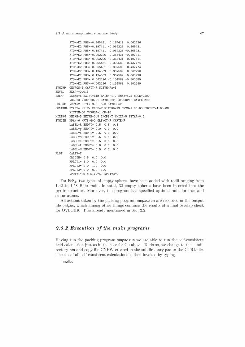
2.3 A more complicated structure: FeS2 67
ATOM=E2 POS=-0.365431 0.197411 0.062226
ATOM=E2 POS=-0.197411 -0.062226 0.365431
ATOM=E2 POS= 0.197411 0.062226 -0.365431
ATOM=E2 POS=-0.062226 0.365431 -0.197411
ATOM=E2 POS= 0.062226 -0.365431 0.197411
ATOM=E2 POS=-0.365431 0.302589 -0.437774
ATOM=E2 POS= 0.365431 -0.302589 0.437774
ATOM=E2 POS=-0.134569 -0.302589 0.062226
ATOM=E2 POS= 0.134569 0.302589 -0.062226
ATOM=E2 POS= 0.062226 -0.134569 -0.302589
ATOM=E2 POS=-0.062226 0.134569 0.302589
SYMGRP GENPOS=T CARTT=F SGSYM=Pa-3
ENVEL EKAP=-0.015
BZSMP NKBAB=6 BZINT=LTM EMIN=-1.0 EMAX=1.5 NDOS=2500
NORD=3 WIDTH=0.01 SAVDOS=F SAVCOOP=F SAVFERM=F
CHARGE NETA=2 EETA=-3.0 -5.0 SAVRHO=F
CONTROL START= QUIT= FREE=F NITBND=99 CNVG=1.0D-08 CNVGET=1.0D-08
NITATM=50 CNVGQA=1.0D-10
MIXING NMIXB=5 BETAB=0.5 INCBB=T NMIXA=5 BETAA=0.5
SYMLIN NPAN=6 NPTS=400 ORBWGT=F CARTE=F
LABEL=R ENDPT= 0.5 0.5 0.5
LABEL=g ENDPT= 0.0 0.0 0.0
LABEL=X ENDPT= 0.5 0.0 0.0
LABEL=M ENDPT= 0.5 0.5 0.0
LABEL=R ENDPT= 0.5 0.5 0.5
LABEL=X ENDPT= 0.0 0.5 0.0
LABEL=M ENDPT= 0.5 0.5 0.0
PLOT CARTV=T
ORIGIN= 0.5 0.0 0.0
RPLOT1= 1.0 0.0 0.0
RPLOT2= 0.0 1.0 0.0
RPLOT3= 0.0 0.0 1.0
NPDIV1=50 NPDIV2=50 NPDIV3=0
For FeS2, two types of empty spheres have been added with radii ranging from1.42 to 1.58 Bohr radii. In total, 32 empty spheres have been inserted into thepyrite structure. Moreover, the program has specified optimal radii for iron andsulfur atoms.
All actions taken by the packing program mnpac.run are recorded in the outputfile outpac, which among other things contains the results of a final overlap checkfor OVLCHK=T as already mentioned in Sec. 2.2.
2.3.2 Execution of the main programs
Having run the packing program mnpac.run we are able to run the self-consistentfield calculation just as in the case for Cu above. To do so, we change to the subdi-rectory nm and copy file CNEW created in the subdirectory pac to the CTRL file.The set of all self-consistent calculations is then invoked by typing
mnall.x

68 2 Execution of the ASW programs: Case studies
at the systems prompt. Already after a few iteration monic outlst6 will tell us thatthe program found a finite indirect band gap, which qualifies iron pyrite as an semi-conductor. Now it is time to browse the input. Going to the end and searchingbackward for the string “Fermi” will put you on the top of a list containing foreach class and partial wave (angular momentum) the amount of charge and thecontribution to the density of states at EF . Of course, for an insulator or semicon-ductor the second column contains only zeros. Special attention deserves the firstcolumn. If compared to the atomic configurations these partial occupations reflectthe charge transfer between the orbitals. If summed over all orbitals of an atom theygive rise to the deviation from the neutrality of an atom, which is given in an extralist above. For most atoms the occupation of the orbital with highest angular mo-mentum is quite small, below 0.1 electron. This guarantess the convergence of theangular momentum expansions of the wave functions. In case the charge containedin the highest l state is above 0.1 a warning is issued. Values up to 0.13 are stillacceptable, otherwise the value given by LMXL= must be increased. In contrast, ifthe numbers for the two highest l orbitals and their sum is below 0.1 electrons, youmight decrease the value set by LMXL= by one. In this context we recall that eachorbital included (of course, there are 2l+1 states for each l) increases the size of thesecular matrix and thus leads to an increase of execution time and memory. Sincethe CPU time scales roughly as the cube of the number of orbitals a reduction of themaximum angular momentum might considerably speed up a calculation. However,such a reduction is allowed only if the above mentioned conditions are fulfilled.
In case you realize during the first iterations that the number of orbitals for aparticular atom should be changed you have to stop execution and delete all atomicfiles (those given by the entries ATOM= in category CLASS). In addition, you mustdelete the file MIX, which holds information about the progress of the iterations andis deleted automatically once self-consistency has been reached. After that adjustthe angular momenta given by the tokens LMXL=. In case you have increasedthe LMXL= values corresponding entries have to be added to tokens CONF= andQVAL=. However, these latter tokens could likewise be completely erased since theprogram creates them automatically. Finally, the calculation can be restarted byagain typing mnall.x at the systems prompt. The complete set of calculations willtake about three quarters of an hour, which is enough for a coffee break!
After completion of all calculations a first impression of the results is obtainedon typing
monic outlst18
at the system prompt, which prints the following summary to screen.
ASW-2.6, program MNSCF started on asterix at Wed, 04 Feb 2009, 20:44:59.
Calculation converged after 10 iteration(s).
Start of Iteration 10
76 irreducible k-points generated from 1331 ( 11, 11, 11).
Fermi energy - MTZ = 0.823867 Ryd.
The system is a semiconductor:
Indirect band gap = 0.037749 Ryd = 0.513595 eV
Mean-square residual: 0.223714D-22
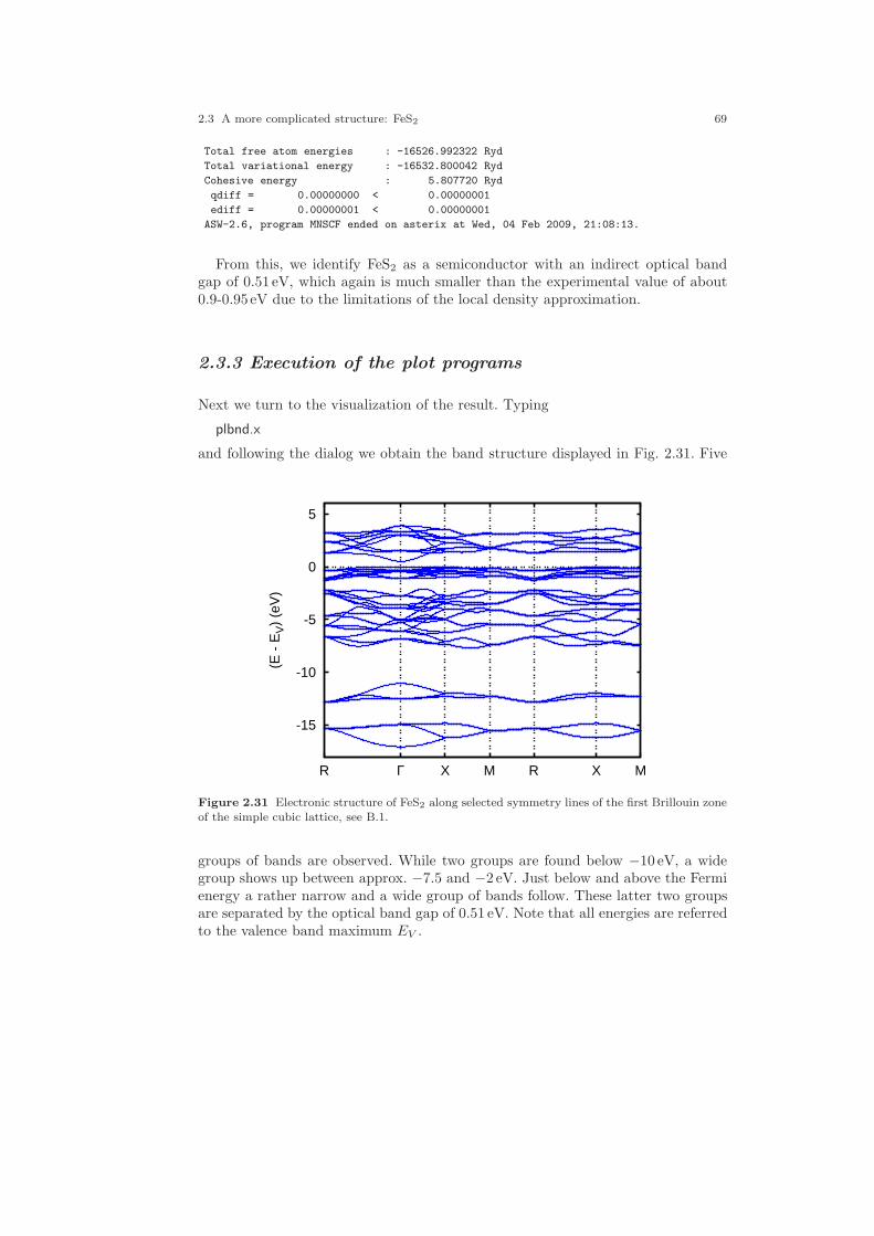
2.3 A more complicated structure: FeS2 69
Total free atom energies : -16526.992322 Ryd
Total variational energy : -16532.800042 Ryd
Cohesive energy : 5.807720 Ryd
qdiff = 0.00000000 < 0.00000001
ediff = 0.00000001 < 0.00000001
ASW-2.6, program MNSCF ended on asterix at Wed, 04 Feb 2009, 21:08:13.
From this, we identify FeS2 as a semiconductor with an indirect optical bandgap of 0.51 eV, which again is much smaller than the experimental value of about0.9-0.95 eV due to the limitations of the local density approximation.
2.3.3 Execution of the plot programs
Next we turn to the visualization of the result. Typing
plbnd.x
and following the dialog we obtain the band structure displayed in Fig. 2.31. Five
-15
-10
-5
0
5
R Γ X M R X M
(E -
EV)
(eV
)
Figure 2.31 Electronic structure of FeS2 along selected symmetry lines of the first Brillouin zoneof the simple cubic lattice, see B.1.
groups of bands are observed. While two groups are found below −10 eV, a widegroup shows up between approx. −7.5 and −2 eV. Just below and above the Fermienergy a rather narrow and a wide group of bands follow. These latter two groupsare separated by the optical band gap of 0.51 eV. Note that all energies are referredto the valence band maximum EV .

70 2 Execution of the ASW programs: Case studies
The predominant orbital character of these five groups is read off from the partialdensities of states as shown in Fig. 2.32. Obviously, the lowest two groups are made
0
5
10
15
20
25
30
35
40
45
-15 -10 -5 0 5
DO
S (
1/eV
)
(E - EV) (eV)
Fe 3dS 3sS 3p
Figure 2.32 Partial densities of states of FeS2.
exclusively from the semicore-like S 3s states, whereas the higher lying states traceback to a mixture of Fe 3d and S 3p bands. The latter orbitals dominate especiallythe wider groups between approx. −7.5 and −2 eV as well as between 2.7 and 4.5 eV.In contrast the sharp peak just below EV is due almost exclusively to the Fe 3dstates.
The previous analysis of the electronic states can be made more detailed bydistinguishing the single p and d components. For the Fe 3d states this is achievedby calling pldos.x again and running through the following dialog.
ASW-2.6, program PLDOS started on asterix at Mon, 09 Feb 2009, 12:15:27.
Copyright (C) 1992-2009 Volker Eyert
Please see file COPYRIGHT for details
All input will be echoed to file PLID.
Enter terminal type:
1 = X-Windows (default)
2 = PC-Screen (vt220-emulation)
3 = suppress terminal output
/
Enter output device (default: 1):
1 = Color postscript
2 = Postscript
3 = PDF (not yet supported)
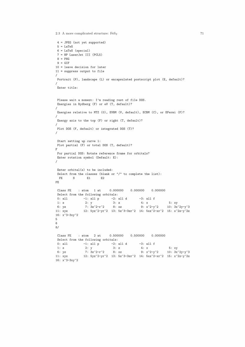
2.3 A more complicated structure: FeS2 71
4 = JPEG (not yet supported)
5 = LaTeX
6 = LaTeX (special)
7 = HP LaserJet III (PCL5)
8 = PNG
9 = GIF
10 = leave decision for later
11 = suppress output to file
/
Portrait (P), landscape (L) or encapsulated postscript plot (E, default)?
/
Enter title:
Please wait a moment: I’m reading rest of file DOS.
Energies in Rydberg (F) or eV (T, default)?
/
Energies relative to MTZ (0), EVBM (V, default), ECBM (C), or EFermi (F)?
/
Energy axis to the top (F) or right (T, default)?
/
Plot DOS (F, default) or integrated DOS (T)?
/
Start setting up curve 1:
Plot partial (F) or total DOS (T, default)?
F
For partial DOS: Rotate reference frame for orbitals?
Enter rotation symbol (Default: E):
/
Enter orbital(s) to be included:
Select from the classes (blank or "/" to complete the list):
FE S E1 E2
FE
Class FE : atom 1 at 0.000000 0.000000 0.000000
Select from the following orbitals:
0: all -1: all p -2: all d -3: all f
1: s 2: y 3: z 4: x 5: xy
6: yz 7: 3z^2-r^2 8: xz 9: x^2-y^2 10: 3x^2y-y^3
11: xyz 12: 5yz^2-yr^2 13: 5z^3-3zr^2 14: 5xz^2-xr^2 15: x^2z-y^2z
16: x^3-3xy^2
5
6
8/
Class FE : atom 2 at 0.500000 0.500000 0.000000
Select from the following orbitals:
0: all -1: all p -2: all d -3: all f
1: s 2: y 3: z 4: x 5: xy
6: yz 7: 3z^2-r^2 8: xz 9: x^2-y^2 10: 3x^2y-y^3
11: xyz 12: 5yz^2-yr^2 13: 5z^3-3zr^2 14: 5xz^2-xr^2 15: x^2z-y^2z
16: x^3-3xy^2

72 2 Execution of the ASW programs: Case studies
/
Class FE : atom 3 at 0.000000 0.500000 0.500000
Select from the following orbitals:
0: all -1: all p -2: all d -3: all f
1: s 2: y 3: z 4: x 5: xy
6: yz 7: 3z^2-r^2 8: xz 9: x^2-y^2 10: 3x^2y-y^3
11: xyz 12: 5yz^2-yr^2 13: 5z^3-3zr^2 14: 5xz^2-xr^2 15: x^2z-y^2z
16: x^3-3xy^2
/
Class FE : atom 4 at 0.500000 0.000000 0.500000
Select from the following orbitals:
0: all -1: all p -2: all d -3: all f
1: s 2: y 3: z 4: x 5: xy
6: yz 7: 3z^2-r^2 8: xz 9: x^2-y^2 10: 3x^2y-y^3
11: xyz 12: 5yz^2-yr^2 13: 5z^3-3zr^2 14: 5xz^2-xr^2 15: x^2z-y^2z
16: x^3-3xy^2
/
Select from the classes (blank or "/" to complete the list):
FE S E1 E2
/
The following orbitals have been selected:
Class FE : atom 1, orbital xy
Class FE : atom 1, orbital yz
Class FE : atom 1, orbital xz
Enter scaling factor (default 1.0):
/
Broadening of this curve (T) or not (F, default)?
/
Select curve style (default: 1) (A * marks styles already selected):
solid/green (1) , dash1/blue (2) ,
dash2/red (3) , dot/magenta (4) ,
dashdot1/cyan (5) , dashdot2/yellow (6) ,
chaindash1/black (7) , chaindash2/coral (8) ,
chaindash3/gray (9) ,
/
Enter curve label ("/" to suppress)
Fe 3d t_{2g}
Please wait a moment: I’m working on this curve.
Set up more curves (T)? Default is F.
T
Start setting up curve 2:
Plot partial (F) or total DOS (T, default)?
F
For partial DOS: Rotate reference frame for orbitals?
Enter rotation symbol (Default: E):
2.3 A more complicated structure: FeS2 73
/
Enter orbital(s) to be included:
Select from the classes (blank or "/" to complete the list):
FE S E1 E2
FE
Class FE : atom 1 at 0.000000 0.000000 0.000000
Select from the following orbitals:
0: all -1: all p -2: all d -3: all f
1: s 2: y 3: z 4: x 5: xy
6: yz 7: 3z^2-r^2 8: xz 9: x^2-y^2 10: 3x^2y-y^3
11: xyz 12: 5yz^2-yr^2 13: 5z^3-3zr^2 14: 5xz^2-xr^2 15: x^2z-y^2z
16: x^3-3xy^2
7
9/
Class FE : atom 2 at 0.500000 0.500000 0.000000
Select from the following orbitals:
0: all -1: all p -2: all d -3: all f
1: s 2: y 3: z 4: x 5: xy
6: yz 7: 3z^2-r^2 8: xz 9: x^2-y^2 10: 3x^2y-y^3
11: xyz 12: 5yz^2-yr^2 13: 5z^3-3zr^2 14: 5xz^2-xr^2 15: x^2z-y^2z
16: x^3-3xy^2
/
Class FE : atom 3 at 0.000000 0.500000 0.500000
Select from the following orbitals:
0: all -1: all p -2: all d -3: all f
1: s 2: y 3: z 4: x 5: xy
6: yz 7: 3z^2-r^2 8: xz 9: x^2-y^2 10: 3x^2y-y^3
11: xyz 12: 5yz^2-yr^2 13: 5z^3-3zr^2 14: 5xz^2-xr^2 15: x^2z-y^2z
16: x^3-3xy^2
/
Class FE : atom 4 at 0.500000 0.000000 0.500000
Select from the following orbitals:
0: all -1: all p -2: all d -3: all f
1: s 2: y 3: z 4: x 5: xy
6: yz 7: 3z^2-r^2 8: xz 9: x^2-y^2 10: 3x^2y-y^3
11: xyz 12: 5yz^2-yr^2 13: 5z^3-3zr^2 14: 5xz^2-xr^2 15: x^2z-y^2z
16: x^3-3xy^2
/
Select from the classes (blank or "/" to complete the list):
FE S E1 E2
/
The following orbitals have been selected:
Class FE : atom 1, orbital 3z^2-r^2
Class FE : atom 1, orbital x^2-y^2
Enter scaling factor (default 1.0):
/

74 2 Execution of the ASW programs: Case studies
Broadening of this curve (T) or not (F, default)?
/
Select curve style (default: 2) (A * marks styles already selected):
solid/green (1) * , dash1/blue (2) ,
dash2/red (3) , dot/magenta (4) ,
dashdot1/cyan (5) , dashdot2/yellow (6) ,
chaindash1/black (7) , chaindash2/coral (8) ,
chaindash3/gray (9) ,
/
Enter curve label ("/" to suppress)
Fe 3d e_g
Please wait a moment: I’m working on this curve.
Set up more curves (T)? Default is F.
/
Center of gravity of DOS curve 1 (Spin 1) - EV : -0.0669 eV
Center of gravity of DOS curve 2 (Spin 1) - EV : -0.1999 eV
Indicate center of gravities (F, default)?
/
Ebot = -16.729321 eV , Etop = 9.529665 eV relative to EV
Emin = -17.000000 eV , Emax = 6.000000 eV relative to EV
Enter new Emin, Emax to change the default:
-9.0
6.0
DOStop = 10.931710 1/eV
DOSmax = 20.000000 1/eV
Enter new DOSmax to change this default:
12.0
Enter energetic position of curve labels ("/" to use default):
-4.0
task 1, total : cpu time: 0.15601 sec
ASW-2.6, program PLDOS ended on asterix at Mon, 09 Feb 2009, 12:15:27.
Please delete files DOS and dos.ps when finished!!!
As a result, we obtain the partial densities of states displayed in Fig. 2.33, whichseparates the Fe 3d partial DOS into their t2g and eg contributions, which in oc-tahedral coordination mediate π and σ type bonding with the respective ligand porbitals. Yet, the t2g and eg manifolds obviously are not clearly separated in energy.In contrast, we observe a mixture of both types of states in all group of bands.Of course, this is due to the rotation of the FeS6 octahedra already discussed inconnection with Fig. 2.29. Hence, in order to correctly assign the t2g and eg orbitalswe have to use a rotated reference frame with the Cartesian axes pointing alongthe Fe-S bonds. With the ASW programs this can be easily achieved. To this end,

2.3 A more complicated structure: FeS2 75
0
2
4
6
8
10
12
-8 -6 -4 -2 0 2 4 6
DO
S (
1/eV
)
(E - EV) (eV)
Fe 3d t2gFe 3d eg
Figure 2.33 Partial Fe 3d densities of states of FeS2.
we enter the above dialog again. However, when being asked to enter the rotationsymbol, we type
R(23)(1,1,0)*R(17)(0,0,1)
which describes the rotation of the octahedra away from the Cartesian axes of theunderlying cubic lattice. As a result, we obtain the partial DOS shown in Fig. 2.34,which indeed reflect the energetical separation of the t2g and eg contributions.
The flexibility of the ASW programs to use rotated reference frames is alsovery helpful for the analysis of the S 3p states. Fig. 2.35 shows the partial 3pdensities of states of two S atoms forming a short bonded pair. Of course, due tothe cubic symmetry, all three contributions are identical. However, using a rotatedreference frame with the z axis pointing along the bond and the x and y axesbeing perpendicular to the bond we arrive at a much different picture. The resultis displayed in Fig. 2.36, which clearly indicates the strong bonding-antibondingsplitting of the σ-bonding orbital pointing along the bond and the weaker splittingof the perpendicular π-bonding orbitals.
Another useful feature is the calculation of orbital weighted band structures,which in the context of the LMTO method, goes under the name
”fatband“. Such
bands structures can be produced by setting ORBWGT=T in category SYMLINand running the program mnbnd.run. As a result, in addition to the file BNDE afile BNDV is obtained, which holds information about the wave functions. Thisinformation can be used to attach to each band at each k point a bar, the widthof which indicates the contribution of a specified orbital to the respective wavefunction. The orbital is selected with the help of the plot program plbnd.run, whichalso allows for rotated reference frames. For FeS2, the results are shown in Figs. 2.37

76 2 Execution of the ASW programs: Case studies
0
2
4
6
8
10
12
-8 -6 -4 -2 0 2 4 6
DO
S (
1/eV
)
(E - EV) (eV)
Fe 3d t2gFe 3d eg
Figure 2.34 Partial Fe 3d densities of states of FeS2.
0
0.5
1
1.5
2
-8 -6 -4 -2 0 2 4 6
DO
S (
1/eV
)
(E - EV) (eV)
S 3px, 3pyS 3pz
Figure 2.35 Partial S 3p densities of states of FeS2.

2.3 A more complicated structure: FeS2 77
0
0.5
1
1.5
2
-8 -6 -4 -2 0 2 4 6
DO
S (
1/eV
)
(E - EV) (eV)
S 3px, 3pyS 3pz
Figure 2.36 Partial S 3p densities of states of FeS2.
and 2.38, which clearly confirm the observation made in the partial DOS, namely
qqqqqqqqqqqqqqq
qqqqqqqqqqqqqqqqqqqqqqqqqqqqqqqqqqqqqqqqqqqqqqqqqqqqqqqqqqqqqqqqqqqqqqqqqqqqqqqqqqqqqqqqqqqqqqqqqqqqqqqqqqqqqqqqqqqqqqqqqqqqqqqqqqqqqqqqqqqqqqqqqqq
qqqqqqqqqqqqqq
qqqqqqqqqqqqqqqqqqqqqqq
qqqqqqqqqqqqqqqqqqqqqqqqqqqqqqqqqqqqqqqqqqqqqqqqqqqqqqqqqqqqqqqqqqqqqqqq
qqqqqqqqqqqqqqqqqqqqqqqqqqqqqqqqqqqqqqqqqqqqqqqqqqqqqqqqqqqqqqqqqqqqqqqqqqqqqqqqqqqqqqqqqqqqqqqqqq
qqqqqqqqqqqqqqqqqqqqqqqqqqqqq
qqqqqqqqqqqqqqqqqqqqqqqqqqqqqqqqqqqqqqqqqqqqqqqqqqqqqqqqqqqqqqq
qqqqqqqqq
qqqqqqqqqqqqqqqqqqqqqqqqqqqqqqqqqqqqqqqqqqqqqqqqqqqqqqqqqqqqqqqqqqqqqqqqqqqqqqqqqqqqqqqqqqqqqqqqqqqqqqqqqqq
qqqqqqqqqqqq
qqqqqqqq
qqqqqqqqqqqqqqqqqqqqqqqqqqqqqqqqqqqqqqqqqqqqqqqqqqqqqqqqqqqqq
qqqqqqqqqqqqq
qqqqqqqqqqqqq
qqqqqqqqqq
qqqqqqqqqqqqq
qqqqqqqqqqqqqqqqqqqqqqqqqqqqqqqqqqqqqqqqqqqqqqqqqqqqqqqqqqqqqqqqqqqqqqqqqqqqqqqqqqqqqqqqq
qqqqqqqqqqqqqqqq
qqqqqqqqqqqqqqqqqqqqqqqqqqqqqqqqqqq
qqqqqqqqqqqqqq
qqqqqqqqqqqqqqqqqqqq
qqqqqqqqqq
qqqqqqqqqqqqq
qqqqqqqqqqqqqqqqqqqqqqqqqqqqqqqqqqqqqqqqqqqqqqqqqqqqqqqqqqqq
qqqqqqqqqqqqqqqqqq
qqqqqqqqqqqqq
qqqqqqqqqqqqqqqq
qqqqqqqqqqqqqqqqqqqqqqqqqqqqqqqqqqqqqqqq
qqqqqqqqqqqqqqqqqq
qqqqqqqqqqqqqqqqqqqqqqqqqqqqq
qqqqqqqqqqqqqqq
qqqqqqqqqqqqqqqqqqqqqqqqqqqqqqqqqqqqqqqqqqqqqqqqqqqqqqqqqqqqqqqqqqqqq
qqqqqqqqqqqq
qqqqqqqqqqqqqqqqqqqqqqqqqqqqqqqqqqqqqqqqqqqqqqqqqqqqqqqqqqqq
qqqqqqqqqqqqqqqqqqqqqqqqqqqqqqqqqqqqqqqqqqqqqqqqqqqqqqqqqqqqqqqqqqqqqqqqqqqqqqqqqqqqqqqqqqqqqqqqqqqqqqqqqqqqqqqqqq
qqqqqqqqqqqqqqqqqqqqqqqqq
qqqqqqqqqqqqqqqqqqqqqqqqqqqqqqqqqqqqqqqqqqqqqqqqqqqqqqqqqqqq
qqqqqqqqqqqqqqqqqqqqqqqqqqqqqqqqqqqqqqqqqqqqqqqqqqqqqqqqqqqqqqqqqqqqqqqqqqqqqqqqqqqqqqqqqqqqqqqqqqqqqqqqqqqqqqqqqqq
qqqqqqqqqqqqqqqqqqqqqqqq
qqqqqqqqqqqqqqqqqqqqqqqqqqqqqqqqqqqqqqqqqqqqqqqqqqqqqqqqqq
qqqqqqqqqqqqqqqqqqqqqqqqqqqqqqqqqqqqqqqqqqqqqqqqqqqqqqqqqqqqqqqqqqqqqqqqqqqqqqqqqqqqqqqqqqqqqqqqqqqqqqqqqqqqqqqqqqqqqqqqqqqqqqq
qqqqqqqqqqqqqq
qqqqqqqqqqqqqqqqqqqqqq
qqqqqqqqqqqq
qqqqqqqqqqqqqqqqqqqqqqqqqqqqqqqqqqqqqqqqqqqqqqqqqqqqqqqqqqqqqqqqqqqqqqqqqqqqqqqqqqqqqqqqqqqqqqqqqqqqqqqqqqqqqqqqqqqqqqqq
qqqqqqqqqqqqq
qqqqqqqqqqqqqqqqqqqqqqqqqqqqqqqq
qqqqqqqqqqqqqqqqqqqqqq
qqqqqqqqqqqq
qqqqqqqqqqqqqqqqqqqqqqqqqqqqqqqqqqqqqqqqqqqqqqqqqqqqqqqqqqqqqqqqqqqqqqqqqqqqqqqqqqqqqqqqqqqqqqqqqqqqqqqqqqqqqqqqq
qqqqqqqqqqqqqqqqqqqqqqqqqqqqqqqqqqqqqqqqqqqqq
qqqqqqq
qqqqqqqqqqqqqqqqqqqq
qqqqqqqqqqqqqqqqqqqqqqqqqqqqqq
qqqqqqqqqqqqq
qqqqqqqqqqqqqqqqqqqqqqqqqqqqqqqqqqqqqqqqqqqqqqqqqqqqqqqqqqqqqqqqqqqqqqqqqqqqqqqqqqqqqqqqqqqqqqqqqqqqqqqqqqqqqqqqqqqqqqqqqqqqqqqqqqqqqqqq
qqqqqqqqqqqqqqqqqqqqqqqqqqqqqqqqqqqqqqqqqqqqqqqqqqqqqqqqqqqqqqqqqqqqqqqqqqqqqqqqqqqqqqqqqqqqqqqqqqqqqqqqqqqqqqqqqqqqqqqqqqqqqqqqqqqqqqqqqqqqqqqqqqqqqqqqqqqqqqqqqqqqqqqqqqqqqqqqqqqqqqqqqqqq
qqqqqqqqqqq
qqqqqqqqqqqqqqqqqqqqqqqqqqqqqqqqqqqqqqqqqqqqqqqqqqqqqqqqqqqqqqqqqqqqqqqqqqqqqqqqqqqqqqqqqqqqqqqqqqqqqqqqqqqqqqq
qqqqqqqqqqqqqqqqqqqqqqqqqqqqqqqqqqqqqqqqqqqqqqqqqqqqqqqqqqqqqqqqqqqqqqqqqqqqqqqqqqqqqqqq
qqqqqqqqqqqqqqqqqqqqqqqqqqqqqqqqqqqqqqqqqqqqqqqqqqqqqqqqqqqqqqqqqqqqqqqqqqqqqqqqqqqqqqqqqqqqqqqqqqqqqqqqqqqqqqq
qqqqqqqqqqqqqqqqqqqqqqqqqqqqqqqqqqqqqqqqqqqqqqqqqqqqqqqqq
qqqqqqqqqqqqqqqqqqqqq
qqqqqqqqqq
qqqqqqqqqqqqqqqqqqqqqqqqqqqqqqqqqqqqqqqqqqqqqqqqqqqq
qqqqqqqqq
qqqqqqqqqqqqqqqqqqqqqqqqqqqqqqqqqqqqqqqqqqqqqqqqqqqqqqqqqqqqqqqqqqqqqqqqqqqqqqqqqqqqqqqqq
qqqqqqqqqqqqqqqqqqqqqqqqqqqqqqqqqqqqqqqqqqqqqqqqq
qqqqqqqqqqqqqqqqqqqqqqqqqqqqqqqqqqqqqqqqqqqqqqqqqqqqqqqqqqqqqqqqqqqqqqqqqq
qqqqqqqqqqqqqqqqqqqqqqqqqqqqqqqqqqqqqqqqqqqqqqqqqqq
qqqqqqqqqqqqqqqqqqqqqqqqqqqqqqqqqqqqqqqqqqqqqqqqqqqqqqqqqqqqqqqqqqqqqqqqqq
qqqqqqqqqqqqqqqqqqqqqqqqqqqqqqqqqqqqqqqqqqqqqqqqqqqqqqqqqqqqqqqqqqqqqqqqqqqqqqqqqqqqqqqqqqqqqqqqqqqqqqqqqqqq
qqqqqqqqqqqqqqqqqqqqqqqqqqqqqqqqqqqqqqqqqqqqqqqqqqqqqqqqqqqqqqqqqqqqqqqqqqqqqqqqqqqqqqqqqqq
qqqqqqqqqqqqqqqqqqqqqq
qqqqqqqqqqqqqqqqqqqqqqqqqqqqqqqqqqqqqqqqq
qqqqqqqqqqqqqqqqqqqqqqqqqqqqqqqqqqqqqqqqqqqqq
qqqqqqqqqqqqqqqqqqqqqqqqqqqqqqqqqqqqqqqqqqqqqqqqqq
qqqqqqqqqqqqqqqqqqqqqqqq
qqqqqqqqqqqqqqqq
q
qqqqqqqqqqqqqqqqqqqqqq
qqqqqqqqqqqqqqqqqqqqqqqqqqqqqqqqqqqqqqqqqqqqqqqqqqqqqqqqqqqqqqqqqqqqqqqqqqqqqqqqqqqqqqqqqq
qqqqqqqqqqqqqqqqqqqqqqqqqqqqqqqqqqqqqqqqqqqqqqqqqqqqqqqqqqqqqqqqqqqqqqqqqqqqqqqqqq
qqqqq
qqqqqqqqqqqqqqqqqqqqqqqqqqqqqqqqqqqqqqqqqqqqqqqqqqqqqqqqqqqqqqqqqqqqqqqqqqqqqqqqqqqqqqqqqqqqqqqqqqqqqqqqqqqqqqqq
qqqqqqqqqqqqqqqqqqqqqqqqqqqqqqqqqqqqqqqqqqqqqqqqqqqqqqqqqqqqqqqqqqqqqqqqqqqqqqqqqqqqqqq
qqqqqqqqqqqqqqqqqqqqqqqqqqqqqqqqqqqqqqqqqqqqqqqqqqqqqqqqqqqqqqqqqqqqqqqqqqqqqqqqqqqqqqqqqqqqqqqq
qqqqqqqqqqqqqqqqqqqqqqqqqqqqqqqqqqqqqqqqqqqqqqqqqqqq
qqqqqqqqqqqqqqqqqqqqqqqqqqqqqqqqqqqqqqqqqqqqqqqqqqq
qqqqqqqqqqqqqqqqqqqqqqqqqqqqqqqqqqqqqqqqqqqqqqqqqqqqqqqqqqqqq
qqqqqqqqqq
qqqqqqqqqq
qqqqqqqqqqqqqqqqqqqqqqqqqqqqqqqqqqqqqqqqqqqqq
qqqqqqqqqqqqqqqqqqqqqqqqqqqq
qqqqqqqqqqqqq
qqqqqqqqqqqqqqqqqqqqqqqqqqq
qqqqq
qqqqqqqqqqqqqqqqqqqqqqqqqqqqqqqqqqqqqqqqqqqqqqqqqqqqqqqqqqqqq
qqqqqqqqqq
qqqqqqqqqq
qqqqqqqqqqqqqqqqqqqqqqqqqqqqqqqqqqqqqqqqqqqqq
qqqqqqqqqqqqqqqqqqqqqqqqqqqqqqqqqqqqqqqqqqqqqqqqqqqqqqqqqqqqqqqqqqqqqqqqq
FeS2 sc, w Fe 3d
R Γ X
E
eV
EV
-2.0
0.0
2.0
4.0
Figure 2.37 Weighted electronic bands of FeS2. The width of the bars given for each bandindicates the contribution due to the Fe 3d orbitals.
that the upper valence band as well as the lower half of the conduction band grouptrace back to the Fe 3d states, while the upper half of the conduction band is moreS 3p like. Yet, the lowest edge of the conduction band near the Γ -point is almostexclusively due to the S 3p orbitals and explains the sensitivity of the optical bandgap to the bond length within the sulfur pair as found in Ref. [409].

78 2 Execution of the ASW programs: Case studies
qqqqqqqqqqqqqqq
qqqqqqqqqqqqqqqqqqqqqqqqqqqqqqqqqqqqqqqqqqqqqqqqqqqqqqqqqqqqqqqqqqqqqqqqqqqqqqqqqqqqqqqqqqqqqqqqqqqqqqqqqqqqqqqqqqqqqqqqqqqqqqqqqqqqqqqqqqqqqqqqqqq
qqqqqqqqqqqqqq
qqqqqqqqqqqqqqqqqqqqqqq
qqqqqqqqqqqqqqqqqqqqqqqqqqqqqqqqqqqqqqqqqqqqqqqqqqqqqqqqqqqqqqqqqqqqqqqq
qqqqqqqqqqqqqqqqqqqqqqqqqqqqqqqqqqqqqqqqqqqqqqqqqqqqqqqqqqqqqqqqqqqqqqqqqqqqqqqqqqqqqqqqqqqqqqqqqq
qqqqqqqqqqqqqqqqqqqqqqqqqqqqq
qqqqqqqqqqqqqqqqqqqqqqqqqqqqqqqqqqqqqqqqqqqqqqqqqqqqqqqqqqqqqqq
qqqqqqqqq
qqqqqqqqqqqqqqqqqqqqqqqqqqqqqqqqqqqqqqqqqqqqqqqqqqqqqqqqqqqqqqqqqqqqqqqqqqqqqqqqqqqqqqqqqqqqqqqqqqqqqqqqqqq
qqqqqqqqqqqq
qqqqqqqq
qqqqqqqqqqqqqqqqqqqqqqqqqqqqqqqqqqqqqqqqqqqqqqqqqqqqqqqqqqqqq
qqqqqqqqqqqqq
qqqqqqqqqqqqq
qqqqqqqqqq
qqqqqqqqqqqqq
qqqqqqqqqqqqqqqqqqqqqqqqqqqqqqqqqqqqqqqqqqqqqqqqqqqqqqqqqqqqqqqqqqqqqqqqqqqqqqqqqqqqqqqqq
qqqqqqqqqqqqqqqq
qqqqqqqqqqqqqqqqqqqqqqqqqqqqqqqqqqq
qqqqqqqqqqqqqq
qqqqqqqqqqqqqqqqqqqq
qqqqqqqqqq
qqqqqqqqqqqqq
qqqqqqqqqqqqqqqqqqqqqqqqqqqqqqqqqqqqqqqqqqqqqqqqqqqqqqqqqqqq
qqqqqqqqqqqqqqqqqq
qqqqqqqqqqqqq
qqqqqqqqqqqqqqqq
qqqqqqqqqqqqqqqqqqqqqqqqqqqqqqqqqqqqqqqq
qqqqqqqqqqqqqqqqqq
qqqqqqqqqqqqqqqqqqqqqqqqqqqqq
qqqqqqqqqqqqqqq
qqqqqqqqqqqqqqqqqqqqqqqqqqqqqqqqqqqqqqqqqqqqqqqqqqqqqqqqqqqqqqqqqqqqq
qqqqqqqqqqqq
qqqqqqqqqqqqqqqqqqqqqqqqqqqqqqqqqqqqqqqqqqqqqqqqqqqqqqqqqqqq
qqqqqqqqqqqqqqqqqqqqqqqqqqqqqqqqqqqqqqqqqqqqqqqqqqqqqqqqqqqqqqqqqqqqqqqqqqqqqqqqqqqqqqqqqqqqqqqqqqqqqqqqqqqqqqqqqq
qqqqqqqqqqqqqqqqqqqqqqqqq
qqqqqqqqqqqqqqqqqqqqqqqqqqqqqqqqqqqqqqqqqqqqqqqqqqqqqqqqqqqq
qqqqqqqqqqqqqqqqqqqqqqqqqqqqqqqqqqqqqqqqqqqqqqqqqqqqqqqqqqqqqqqqqqqqqqqqqqqqqqqqqqqqqqqqqqqqqqqqqqqqqqqqqqqqqqqqqqq
qqqqqqqqqqqqqqqqqqqqqqqq
qqqqqqqqqqqqqqqqqqqqqqqqqqqqqqqqqqqqqqqqqqqqqqqqqqqqqqqqqq
qqqqqqqqqqqqqqqqqqqqqqqqqqqqqqqqqqqqqqqqqqqqqqqqqqqqqqqqqqqqqqqqqqqqqqqqqqqqqqqqqqqqqqqqqqqqqqqqqqqqqqqqqqqqqqqqqqqqqqqqqqqqqqq
qqqqqqqqqqqqqq
qqqqqqqqqqqqqqqqqqqqqq
qqqqqqqqqqqq
qqqqqqqqqqqqqqqqqqqqqqqqqqqqqqqqqqqqqqqqqqqqqqqqqqqqqqqqqqqqqqqqqqqqqqqqqqqqqqqqqqqqqqqqqqqqqqqqqqqqqqqqqqqqqqqqqqqqqqqq
qqqqqqqqqqqqq
qqqqqqqqqqqqqqqqqqqqqqqqqqqqqqqq
qqqqqqqqqqqqqqqqqqqqqq
qqqqqqqqqqqq
qqqqqqqqqqqqqqqqqqqqqqqqqqqqqqqqqqqqqqqqqqqqqqqqqqqqqqqqqqqqqqqqqqqqqqqqqqqqqqqqqqqqqqqqqqqqqqqqqqqqqqqqqqqqqqqqq
qqqqqqqqqqqqqqqqqqqqqqqqqqqqqqqqqqqqqqqqqqqqq
qqqqqqq
qqqqqqqqqqqqqqqqqqqq
qqqqqqqqqqqqqqqqqqqqqqqqqqqqqq
qqqqqqqqqqqqq
qqqqqqqqqqqqqqqqqqqqqqqqqqqqqqqqqqqqqqqqqqqqqqqqqqqqqqqqqqqqqqqqqqqqqqqqqqqqqqqqqqqqqqqqqqqqqqqqqqqqqqqqqqqqqqqqqqqqqqqqqqqqqqqqqqqqqqqq
qqqqqqqqqqqqqqqqqqqqqqqqqqqqqqqqqqqqqqqqqqqqqqqqqqqqqqqqqqqqqqqqqqqqqqqqqqqqqqqqqqqqqqqqqqqqqqqqqqqqqqqqqqqqqqqqqqqqqqqqqqqqqqqqqqqqqqqqqqqqqqqqqqqqqqqqqqqqqqqqqqqqqqqqqqqqqqqqqqqqqqqqqqqq
qqqqqqqqqqq
qqqqqqqqqqqqqqqqqqqqqqqqqqqqqqqqqqqqqqqqqqqqqqqqqqqqqqqqqqqqqqqqqqqqqqqqqqqqqqqqqqqqqqqqqqqqqqqqqqqqqqqqqqqqqqq
qqqqqqqqqqqqqqqqqqqqqqqqqqqqqqqqqqqqqqqqqqqqqqqqqqqqqqqqqqqqqqqqqqqqqqqqqqqqqqqqqqqqqqqq
qqqqqqqqqqqqqqqqqqqqqqqqqqqqqqqqqqqqqqqqqqqqqqqqqqqqqqqqqqqqqqqqqqqqqqqqqqqqqqqqqqqqqqqqqqqqqqqqqqqqqqqqqqqqqqq
qqqqqqqqqqqqqqqqqqqqqqqqqqqqqqqqqqqqqqqqqqqqqqqqqqqqqqqqq
qqqqqqqqqqqqqqqqqqqqq
qqqqqqqqqq
qqqqqqqqqqqqqqqqqqqqqqqqqqqqqqqqqqqqqqqqqqqqqqqqqqqq
qqqqqqqqq
qqqqqqqqqqqqqqqqqqqqqqqqqqqqqqqqqqqqqqqqqqqqqqqqqqqqqqqqqqqqqqqqqqqqqqqqqqqqqqqqqqqqqqqqq
qqqqqqqqqqqqqqqqqqqqqqqqqqqqqqqqqqqqqqqqqqqqqqqqq
qqqqqqqqqqqqqqqqqqqqqqqqqqqqqqqqqqqqqqqqqqqqqqqqqqqqqqqqqqqqqqqqqqqqqqqqqq
qqqqqqqqqqqqqqqqqqqqqqqqqqqqqqqqqqqqqqqqqqqqqqqqqqq
qqqqqqqqqqqqqqqqqqqqqqqqqqqqqqqqqqqqqqqqqqqqqqqqqqqqqqqqqqqqqqqqqqqqqqqqqq
qqqqqqqqqqqqqqqqqqqqqqqqqqqqqqqqqqqqqqqqqqqqqqqqqqqqqqqqqqqqqqqqqqqqqqqqqqqqqqqqqqqqqqqqqqqqqqqqqqqqqqqqqqqq
qqqqqqqqqqqqqqqqqqqqqqqqqqqqqqqqqqqqqqqqqqqqqqqqqqqqqqqqqqqqqqqqqqqqqqqqqqqqqqqqqqqqqqqqqqq
qqqqqqqqqqqqqqqqqqqqqq
qqqqqqqqqqqqqqqqqqqqqqqqqqqqqqqqqqqqqqqqq
qqqqqqqqqqqqqqqqqqqqqqqqqqqqqqqqqqqqqqqqqqqqq
qqqqqqqqqqqqqqqqqqqqqqqqqqqqqqqqqqqqqqqqqqqqqqqqqq
qqqqqqqqqqqqqqqqqqqqqqqq
qqqqqqqqqqqqqqqq
q
qqqqqqqqqqqqqqqqqqqqqq
qqqqqqqqqqqqqqqqqqqqqqqqqqqqqqqqqqqqqqqqqqqqqqqqqqqqqqqqqqqqqqqqqqqqqqqqqqqqqqqqqqqqqqqqqq
qqqqqqqqqqqqqqqqqqqqqqqqqqqqqqqqqqqqqqqqqqqqqqqqqqqqqqqqqqqqqqqqqqqqqqqqqqqqqqqqqq
qqqqq
qqqqqqqqqqqqqqqqqqqqqqqqqqqqqqqqqqqqqqqqqqqqqqqqqqqqqqqqqqqqqqqqqqqqqqqqqqqqqqqqqqqqqqqqqqqqqqqqqqqqqqqqqqqqqqqq
qqqqqqqqqqqqqqqqqqqqqqqqqqqqqqqqqqqqqqqqqqqqqqqqqqqqqqqqqqqqqqqqqqqqqqqqqqqqqqqqqqqqqqq
qqqqqqqqqqqqqqqqqqqqqqqqqqqqqqqqqqqqqqqqqqqqqqqqqqqqqqqqqqqqqqqqqqqqqqqqqqqqqqqqqqqqqqqqqqqqqqqq
qqqqqqqqqqqqqqqqqqqqqqqqqqqqqqqqqqqqqqqqqqqqqqqqqqqq
qqqqqqqqqqqqqqqqqqqqqqqqqqqqqqqqqqqqqqqqqqqqqqqqqqq
qqqqqqqqqqqqqqqqqqqqqqqqqqqqqqqqqqqqqqqqqqqqqqqqqqqqqqqqqqqqq
qqqqqqqqqq
qqqqqqqqqq
qqqqqqqqqqqqqqqqqqqqqqqqqqqqqqqqqqqqqqqqqqqqq
qqqqqqqqqqqqqqqqqqqqqqqqqqqq
qqqqqqqqqqqqq
qqqqqqqqqqqqqqqqqqqqqqqqqqq
qqqqq
qqqqqqqqqqqqqqqqqqqqqqqqqqqqqqqqqqqqqqqqqqqqqqqqqqqqqqqqqqqqq
qqqqqqqqqq
qqqqqqqqqq
qqqqqqqqqqqqqqqqqqqqqqqqqqqqqqqqqqqqqqqqqqqqq
qqqqqqqqqqqqqqqqqqqqqqqqqqqqqqqqqqqqqqqqqqqqqqqqqqqqqqqqqqqqqqqqqqqqqqqqq
FeS2 sc, w S 3p
R Γ X
E
eV
EV
-2.0
0.0
2.0
4.0
Figure 2.38 Weighted electronic bands of FeS2. The width of the bars given for each bandindicates the contribution due to the S 3p orbitals.
2.3.4 Electron densities and potential
We start discussion of the electron densities and the effective potential by calling
mnrho.x
before the self-consistent calculations start. As outlined previously, this will gen-erate a file FREE, which holds the electron densities and the potential resultingfrom an assembly of overlapping free atoms in the plot plane defined by the tokensORIGIN=, RPLOT1=, and RPLOT2=. By typing
plrho.x
at the systems prompt this file can be used to generate the overlapping free atompotential, which is displayed in Fig. 2.39. where we identify the potential well ofthe sulfur pair in the middle of the plot. This potential is to be contrasted by theself-consistently calculated potential, which can be accessed by running mnrho.xat the very end and going through the plot routine again, this time for file RHO.The result is given in Fig. 2.40. Indeed, both potentials are hard to distinguish. Thisreflects the observation by Mattheiss mentioned in Sec. 2.2 that the self-consistentlycalculated electron densities and potential are almost identical to that arising froman overlapping free atom calculation. Of course, the quantities are modified bythe formation of the chemical bonds on approaching self-consistency as has beendiscussed with respect to the valence electron density of Si as displayed in Fig. 2.16and 2.20. However, as compared to the total valence electron density, these densitychanges are rather small and, hence, the overlapping free atom quanities serve as agood starting point.
Next we turn to the electron density and, again using plrho.x plot the valenceelectron density, which is displayed in Fig. 2.41. In addition, we show in Fig. 2.42 the
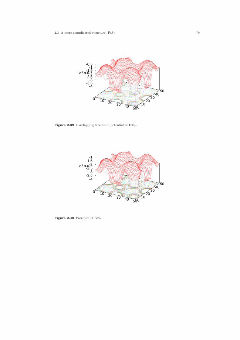
2.3 A more complicated structure: FeS2 79
0 10 20 30 40 50 0 10
20 30
40 50
-4-3.5
-3-2.5
-2-1.5
-1-0.5
v / a.u.
Figure 2.39 Overlapping free atom potential of FeS2.
0 10 20 30 40 50 0 10
20 30
40 50
-4-3.5
-3-2.5
-2-1.5
-1
v / a.u.
Figure 2.40 Potential of FeS2.

80 2 Execution of the ASW programs: Case studies
0 10 20 30 40 50 0 10
20 30
40 50
0 0.02 0.04 0.06 0.08 0.1 0.12 0.14 0.16 0.18 0.2 0.22
ρv / a.u.
Figure 2.41 Valence electron density of FeS2.
0 10 20 30 40 50 0 10
20 30
40 50
-0.3-0.2-0.1
0 0.1 0.2 0.3
-∇ 2ρv / a.u.
Figure 2.42 Negative Laplacian of the valence electron density of FeS2.

2.3 A more complicated structure: FeS2 81
negative Laplacian, which allows to display more details than the electron densityitself.
2.3.5 Structure optimization
In closing this section we turn to full structure optimization for FeS2. According tothe discussion at the begining of this section as well as to the entries in the CTRLfile, the pyrite structure depends on two parameters, namely the lattice constantand the sulfur parameter u, which determines the position of the S atoms at (u, u, u)and the symmetry related positions. The subsequent optimization proceeds in twosteps.
First, we optimize the lattice constant by calling
mnblk.x
after having properly prepared both the CTRL file and this shell script along thelines mentioned in Sec. 2.1.8. After successful completion of all calculations, we runthe shell script prblk, which will extract the cell volumes and total energies from allthe output files and write them to a small file called BLK. This file in turn is usedby the plot routine called by the command
plblk.x
and results in the plot given in Fig. 2.43. Here, the dashed line grows out of a third-order Birch-Murnaghan fit [46, 269, 270]. The cell volume corresponds to a latticeconstant a0 = 10.199aB, which is in good agreement with experimental values. Acomplete list of published lattice constants is given in Tab. 2.1, which reflects the
a0 method reference
10.28 NCPP Zeng and Holzwarth ’94
10.02 FPLO Opahle et al. ’99
10.17 CRYSTAL98 Muscat et al. ’02
9.92 CASTEP Muscat et al. ’02
10.20 FPASW present work
10.23 exp. Finklea et al. ’76
10.22 exp. Will et al. ’84
10.23 exp. Stevens et al. ’91
Table 2.1 Calculated and measured lattice constants of FeS2.
high quality of the ASW method. This is underlined by a comparison of theoreticaland experimental bulk moduli as given in Tab. 2.2,
Next we turn to the internal sulfur parameter. It is optimized following thesame procedure as in the frozen phonon calculation for Si in Sec. 2.2. Hence, (after
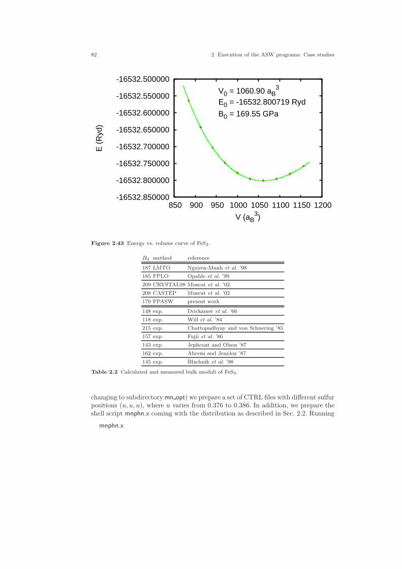
82 2 Execution of the ASW programs: Case studies
-16532.850000
-16532.800000
-16532.750000
-16532.700000
-16532.650000
-16532.600000
-16532.550000
-16532.500000
850 900 950 1000 1050 1100 1150 1200
E (
Ryd
)
V (aB3)
V0 = 1060.90 aB3
E0 = -16532.800719 Ryd
B0 = 169.55 GPa
Figure 2.43 Energy vs. volume curve of FeS2.
B0 method reference
187 LMTO Nguyen-Manh et al. ’98
185 FPLO Opahle et al. ’99
209 CRYSTAL98 Muscat et al. ’02
208 CASTEP Muscat et al. ’02
170 FPASW present work
148 exp. Drickamer et al. ’66
118 exp. Will et al. ’84
215 exp. Chattopadhyay and von Schnering ’85
157 exp. Fujii et al. ’86
143 exp. Jephcoat and Olson ’87
162 exp. Ahrens and Jeanloz ’87
145 exp. Blachnik et al. ’98
Table 2.2 Calculated and measured bulk moduli of FeS2.
changing to subdirectory mn opt) we prepare a set of CTRL files with different sulfurpositions (u, u, u), where u varies from 0.376 to 0.386. In addition, we prepare theshell script mnphn.x coming with the distribution as described in Sec. 2.2. Running
mnphn.x

2.3 A more complicated structure: FeS2 83
will then produce a set of output files, from which sulfur positions and total enrgiescan be extracted and stored in file PHN by the shell script prphn. Finally, the resultis plotted by invoking the shell script
plphn.x
which leads to the results displayed in Fig. 2.44. Again, we contrast the calculated
-16532.740000
-16532.738000
-16532.736000
-16532.734000
-16532.732000
-16532.730000
0.376 0.378 0.38 0.382 0.384 0.386
E (
Ryd
)
u
u0 = 0.380403
E0 = -16532.738979 Ryd
k0 = 640.97 Ryd/u2
a0 = 2426.13 Ryd/u3
Figure 2.44 Energy vs. sulfur position of FeS2.
u parameter with those growing out of related calculations and experimental valuesin Tab. 2.3 and again the result gained by the ASW method is not too bad.
Just in order to demonstrate the striking superiority of the full potential de-scription, we complement Fig. 2.44 by Fig. 2.45, which was calculated using version2.2, which is still based on the ASA but includes the nonspherical contributionsto the electron densities and potential. Nevertheless, according to Fig. 2.45, this isnot sufficient for the calculation of accurate total energies since the atomic spheresstill overlap. Instead, the total energy has to be calculated with nonoverlappingmuffin-tin spheres as it is done in the new versions of the ASW code.
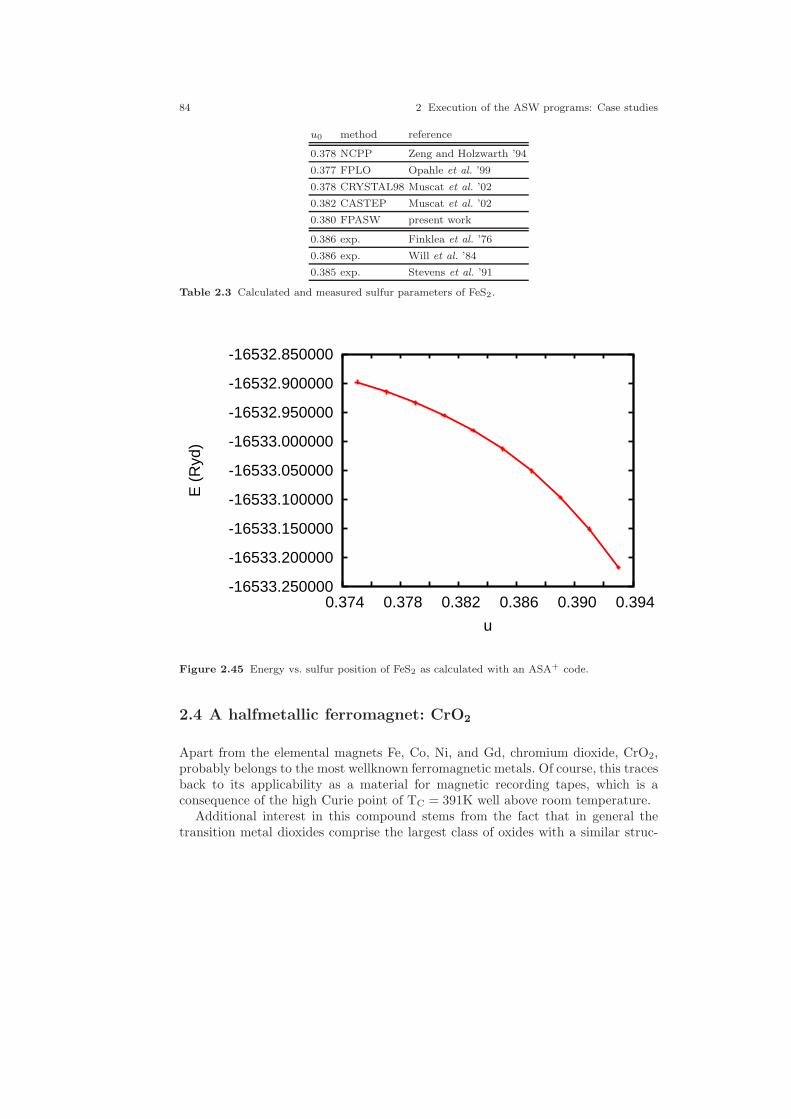
84 2 Execution of the ASW programs: Case studies
u0 method reference
0.378 NCPP Zeng and Holzwarth ’94
0.377 FPLO Opahle et al. ’99
0.378 CRYSTAL98 Muscat et al. ’02
0.382 CASTEP Muscat et al. ’02
0.380 FPASW present work
0.386 exp. Finklea et al. ’76
0.386 exp. Will et al. ’84
0.385 exp. Stevens et al. ’91
Table 2.3 Calculated and measured sulfur parameters of FeS2.
-16533.250000
-16533.200000
-16533.150000
-16533.100000
-16533.050000
-16533.000000
-16532.950000
-16532.900000
-16532.850000
0.374 0.378 0.382 0.386 0.390 0.394
E (
Ryd
)
u
Figure 2.45 Energy vs. sulfur position of FeS2 as calculated with an ASA+ code.
2.4 A halfmetallic ferromagnet: CrO2
Apart from the elemental magnets Fe, Co, Ni, and Gd, chromium dioxide, CrO2,probably belongs to the most wellknown ferromagnetic metals. Of course, this tracesback to its applicability as a material for magnetic recording tapes, which is aconsequence of the high Curie point of TC = 391K well above room temperature.
Additional interest in this compound stems from the fact that in general thetransition metal dioxides comprise the largest class of oxides with a similar struc-
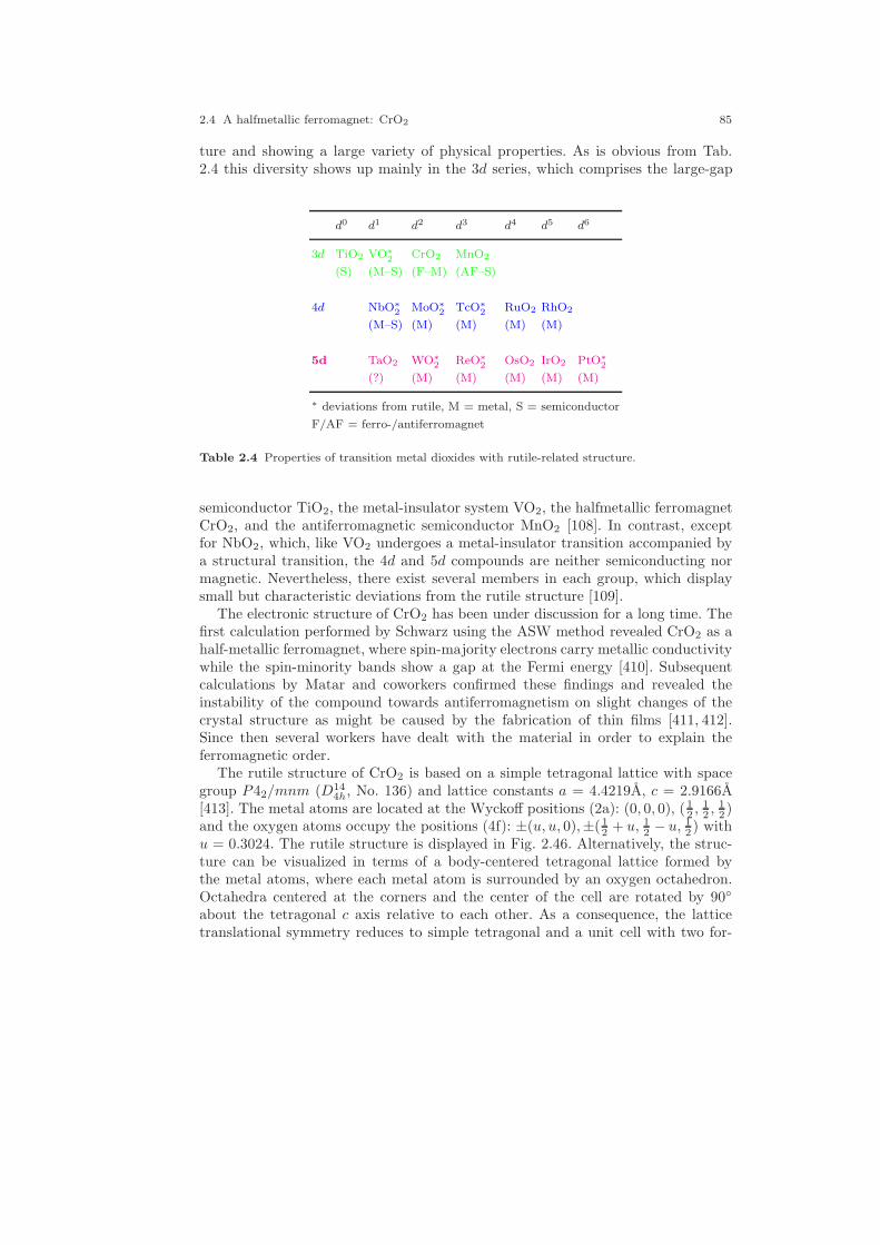
2.4 A halfmetallic ferromagnet: CrO2 85
ture and showing a large variety of physical properties. As is obvious from Tab.2.4 this diversity shows up mainly in the 3d series, which comprises the large-gap
d0 d1 d2 d3 d4 d5 d6
3d TiO2 VO∗
2CrO2 MnO2
(S) (M–S) (F–M) (AF–S)
4d NbO∗
2MoO∗
2TcO∗
2RuO2 RhO2
(M–S) (M) (M) (M) (M)
5d TaO2 WO∗
2ReO∗
2OsO2 IrO2 PtO∗
2
(?) (M) (M) (M) (M) (M)
∗ deviations from rutile, M = metal, S = semiconductor
F/AF = ferro-/antiferromagnet
Table 2.4 Properties of transition metal dioxides with rutile-related structure.
semiconductor TiO2, the metal-insulator system VO2, the halfmetallic ferromagnetCrO2, and the antiferromagnetic semiconductor MnO2 [108]. In contrast, exceptfor NbO2, which, like VO2 undergoes a metal-insulator transition accompanied bya structural transition, the 4d and 5d compounds are neither semiconducting normagnetic. Nevertheless, there exist several members in each group, which displaysmall but characteristic deviations from the rutile structure [109].
The electronic structure of CrO2 has been under discussion for a long time. Thefirst calculation performed by Schwarz using the ASW method revealed CrO2 as ahalf-metallic ferromagnet, where spin-majority electrons carry metallic conductivitywhile the spin-minority bands show a gap at the Fermi energy [410]. Subsequentcalculations by Matar and coworkers confirmed these findings and revealed theinstability of the compound towards antiferromagnetism on slight changes of thecrystal structure as might be caused by the fabrication of thin films [411, 412].Since then several workers have dealt with the material in order to explain theferromagnetic order.
The rutile structure of CrO2 is based on a simple tetragonal lattice with spacegroup P42/mnm (D14
4h, No. 136) and lattice constants a = 4.4219A, c = 2.9166A[413]. The metal atoms are located at the Wyckoff positions (2a): (0, 0, 0), (1
2, 1
2, 1
2)
and the oxygen atoms occupy the positions (4f): ±(u, u, 0),±(1
2+ u, 1
2− u, 1
2) with
u = 0.3024. The rutile structure is displayed in Fig. 2.46. Alternatively, the struc-ture can be visualized in terms of a body-centered tetragonal lattice formed bythe metal atoms, where each metal atom is surrounded by an oxygen octahedron.Octahedra centered at the corners and the center of the cell are rotated by 90◦
about the tetragonal c axis relative to each other. As a consequence, the latticetranslational symmetry reduces to simple tetragonal and a unit cell with two for-
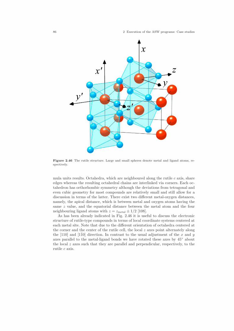
86 2 Execution of the ASW programs: Case studies
Figure 2.46 The rutile structure. Large and small spheres denote metal and ligand atoms, re-spectively.
mula units results. Octahedra, which are neighboured along the rutile c axis, shareedges whereas the resulting octahedral chains are interlinked via corners. Each oc-tahedron has orthorhombic symmetry although the deviations from tetragonal andeven cubic geometry for most compounds are relatively small and still allow for adiscussion in terms of the latter. There exist two different metal-oxygen distances,namely, the apical distance, which is between metal and oxygen atoms having thesame z value, and the equatorial distance between the metal atom and the fourneighbouring ligand atoms with z = zmetal ± 1/2 [108].
As has been already indicated in Fig. 2.46 it is useful to discuss the electronicstructure of rutile-type compounds in terms of local coordinate systems centered ateach metal site. Note that due to the different orientation of octahedra centered atthe corner and the center of the rutile cell, the local z axes point alternately alongthe [110] and [110] direction. In contrast to the usual adjustment of the x and yaxes parallel to the metal-ligand bonds we have rotated these axes by 45◦ aboutthe local z axes such that they are parallel and perpendicular, respectively, to therutile c axis.
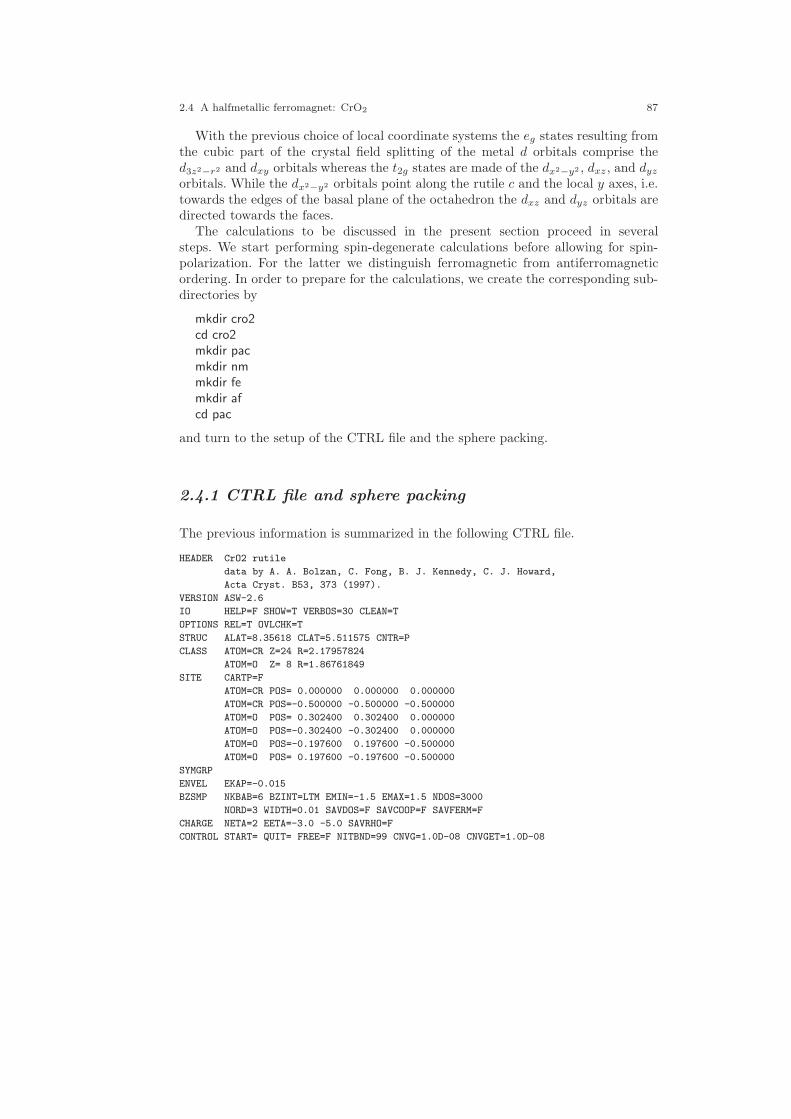
2.4 A halfmetallic ferromagnet: CrO2 87
With the previous choice of local coordinate systems the eg states resulting fromthe cubic part of the crystal field splitting of the metal d orbitals comprise thed3z2−r2 and dxy orbitals whereas the t2g states are made of the dx2−y2 , dxz , and dyz
orbitals. While the dx2−y2 orbitals point along the rutile c and the local y axes, i.e.towards the edges of the basal plane of the octahedron the dxz and dyz orbitals aredirected towards the faces.
The calculations to be discussed in the present section proceed in severalsteps. We start performing spin-degenerate calculations before allowing for spin-polarization. For the latter we distinguish ferromagnetic from antiferromagneticordering. In order to prepare for the calculations, we create the corresponding sub-directories by
mkdir cro2cd cro2mkdir pacmkdir nmmkdir femkdir afcd pac
and turn to the setup of the CTRL file and the sphere packing.
2.4.1 CTRL file and sphere packing
The previous information is summarized in the following CTRL file.
HEADER CrO2 rutile
data by A. A. Bolzan, C. Fong, B. J. Kennedy, C. J. Howard,
Acta Cryst. B53, 373 (1997).
VERSION ASW-2.6
IO HELP=F SHOW=T VERBOS=30 CLEAN=T
OPTIONS REL=T OVLCHK=T
STRUC ALAT=8.35618 CLAT=5.511575 CNTR=P
CLASS ATOM=CR Z=24 R=2.17957824
ATOM=O Z= 8 R=1.86761849
SITE CARTP=F
ATOM=CR POS= 0.000000 0.000000 0.000000
ATOM=CR POS=-0.500000 -0.500000 -0.500000
ATOM=O POS= 0.302400 0.302400 0.000000
ATOM=O POS=-0.302400 -0.302400 0.000000
ATOM=O POS=-0.197600 0.197600 -0.500000
ATOM=O POS= 0.197600 -0.197600 -0.500000
SYMGRP
ENVEL EKAP=-0.015
BZSMP NKBAB=6 BZINT=LTM EMIN=-1.5 EMAX=1.5 NDOS=3000
NORD=3 WIDTH=0.01 SAVDOS=F SAVCOOP=F SAVFERM=F
CHARGE NETA=2 EETA=-3.0 -5.0 SAVRHO=F
CONTROL START= QUIT= FREE=F NITBND=99 CNVG=1.0D-08 CNVGET=1.0D-08
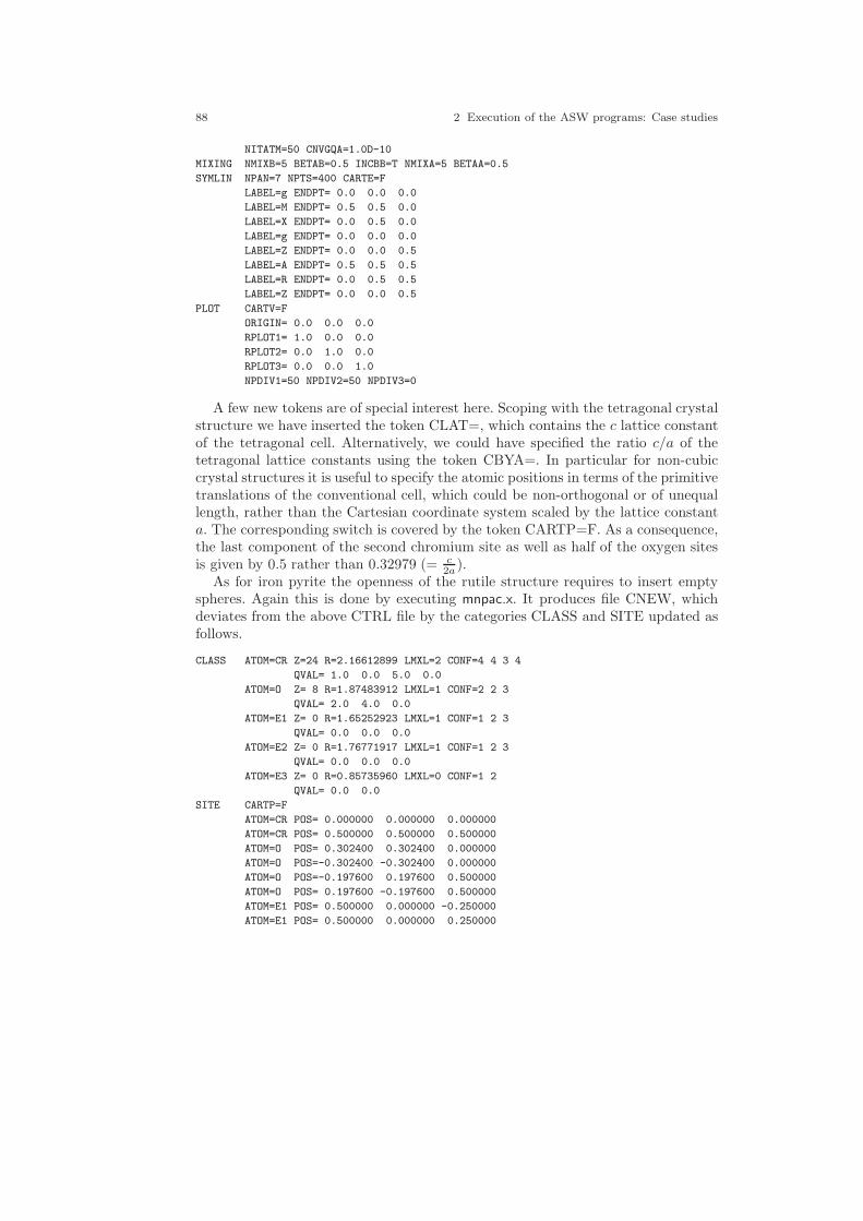
88 2 Execution of the ASW programs: Case studies
NITATM=50 CNVGQA=1.0D-10
MIXING NMIXB=5 BETAB=0.5 INCBB=T NMIXA=5 BETAA=0.5
SYMLIN NPAN=7 NPTS=400 CARTE=F
LABEL=g ENDPT= 0.0 0.0 0.0
LABEL=M ENDPT= 0.5 0.5 0.0
LABEL=X ENDPT= 0.0 0.5 0.0
LABEL=g ENDPT= 0.0 0.0 0.0
LABEL=Z ENDPT= 0.0 0.0 0.5
LABEL=A ENDPT= 0.5 0.5 0.5
LABEL=R ENDPT= 0.0 0.5 0.5
LABEL=Z ENDPT= 0.0 0.0 0.5
PLOT CARTV=F
ORIGIN= 0.0 0.0 0.0
RPLOT1= 1.0 0.0 0.0
RPLOT2= 0.0 1.0 0.0
RPLOT3= 0.0 0.0 1.0
NPDIV1=50 NPDIV2=50 NPDIV3=0
A few new tokens are of special interest here. Scoping with the tetragonal crystalstructure we have inserted the token CLAT=, which contains the c lattice constantof the tetragonal cell. Alternatively, we could have specified the ratio c/a of thetetragonal lattice constants using the token CBYA=. In particular for non-cubiccrystal structures it is useful to specify the atomic positions in terms of the primitivetranslations of the conventional cell, which could be non-orthogonal or of unequallength, rather than the Cartesian coordinate system scaled by the lattice constanta. The corresponding switch is covered by the token CARTP=F. As a consequence,the last component of the second chromium site as well as half of the oxygen sitesis given by 0.5 rather than 0.32979 (= c
2a).
As for iron pyrite the openness of the rutile structure requires to insert emptyspheres. Again this is done by executing mnpac.x. It produces file CNEW, whichdeviates from the above CTRL file by the categories CLASS and SITE updated asfollows.
CLASS ATOM=CR Z=24 R=2.16612899 LMXL=2 CONF=4 4 3 4
QVAL= 1.0 0.0 5.0 0.0
ATOM=O Z= 8 R=1.87483912 LMXL=1 CONF=2 2 3
QVAL= 2.0 4.0 0.0
ATOM=E1 Z= 0 R=1.65252923 LMXL=1 CONF=1 2 3
QVAL= 0.0 0.0 0.0
ATOM=E2 Z= 0 R=1.76771917 LMXL=1 CONF=1 2 3
QVAL= 0.0 0.0 0.0
ATOM=E3 Z= 0 R=0.85735960 LMXL=0 CONF=1 2
QVAL= 0.0 0.0
SITE CARTP=F
ATOM=CR POS= 0.000000 0.000000 0.000000
ATOM=CR POS= 0.500000 0.500000 0.500000
ATOM=O POS= 0.302400 0.302400 0.000000
ATOM=O POS=-0.302400 -0.302400 0.000000
ATOM=O POS=-0.197600 0.197600 0.500000
ATOM=O POS= 0.197600 -0.197600 0.500000
ATOM=E1 POS= 0.500000 0.000000 -0.250000
ATOM=E1 POS= 0.500000 0.000000 0.250000

2.4 A halfmetallic ferromagnet: CrO2 89
ATOM=E1 POS= 0.000000 -0.500000 -0.250000
ATOM=E1 POS= 0.000000 -0.500000 0.250000
ATOM=E2 POS= 0.318691 -0.318691 0.000000
ATOM=E2 POS=-0.318691 0.318691 0.000000
ATOM=E2 POS=-0.181309 -0.181309 -0.500000
ATOM=E2 POS= 0.181309 0.181309 -0.500000
ATOM=E3 POS= 0.313120 -0.055474 0.000000
ATOM=E3 POS=-0.313120 0.055474 0.000000
ATOM=E3 POS=-0.186880 -0.444526 -0.500000
ATOM=E3 POS= 0.186880 0.444526 0.500000
ATOM=E3 POS= 0.055474 -0.313120 0.000000
ATOM=E3 POS=-0.055474 0.313120 0.000000
ATOM=E3 POS=-0.444526 -0.186880 -0.500000
ATOM=E3 POS= 0.444526 0.186880 -0.500000
To be specific, 16 empty spheres of three different types have been added withradii ranging from 0.85 to 1.77 aB.
2.4.2 Spin-degenerate calculations
With the complete CTRL file at hand we are in a position to perform the self-consistent calculations for non-magnetic CrO2 by typing
mnall.x
at the systems prompt. Although it is possible to start with the spin-polarized calcu-lations rightaway, it is recommended to do the calculations for the spin-degeneratecase in advance. First, these calculations need about half the execution time since thesecular matrix has to be constructed and solved for one spin direction only. Owingto the restart facility of the ASW program mnscf.run the subsequent spin-polarizedcalculations can start away with the converged files of the spin-degenerate calcula-tions rather then starting from scratch. Second, the result for the spin-degeneratecase establish a reference, to which the results of the spin-polarized calculation canbe compared. In particular, by checking the total energies we are able find out therelative stability of the ferromagnetic state.
After convergence has been achieved monic outlst18 summarizes the results asfollows.
ASW-2.6, program MNSCF started on asterix at Thu, 05 Feb 2009, 22:53:46.
Calculation converged after 13 iteration(s).
Start of Iteration 13
396 irreducible k-points generated from 4116 ( 14, 14, 21).
Fermi energy - MTZ = 0.758139 Ryd
The system is a metal:
DOS at Fermi energy: 124.457446 1/Ryd
Gamma * (f.u./cell): 21.561888 mJ/(mole*K**2)
Mean-square residual: 0.760111D-23
Total free atom energies : -4790.190932 Ryd
Total variational energy : -4793.995502 Ryd

90 2 Execution of the ASW programs: Case studies
Cohesive energy : 3.804569 Ryd
qdiff = 0.00000000 < 0.00000001
ediff = 0.00000001 < 0.00000001
ASW-2.6, program MNSCF ended on asterix at Thu, 05 Feb 2009, 23:03:58.
In particular, non-magnetic CrO2 turns out to be a metal with a rather highdensity of states at EF . Within the framework of the Stoner theory of magnetismthis is interpreted as a precursor of the ferromagnetic order of this material. We dis-play in Fig. 2.47 the electronic states along selected high symmetry lines within the
-8
-6
-4
-2
0
2
4
6
8
Γ M X Γ Z A R Z
(E -
EF)
(eV
)
Figure 2.47 Electronic bands of CrO2 along selected symmetry lines within the first Brillouinzone of the simple tetragonal lattice, Fig. B.5(a).
first Brillouin zone of the simple tetragonal lattice, Fig. B.5(a). The correspondingdensity of states (DOS) is generated with the plot routine pldos.run, which opensthe follwoing dialog.
ASW-2.6, program PLDOS started on asterix at Mon, 09 Feb 2009, 19:46:51.
Copyright (C) 1992-2009 Volker Eyert
Please see file COPYRIGHT for details
All input will be echoed to file PLID.
Enter terminal type:
1 = X-Windows (default)
2 = PC-Screen (vt220-emulation)
3 = suppress terminal output
/

2.4 A halfmetallic ferromagnet: CrO2 91
Enter output device (default: 1):
1 = Color postscript
2 = Postscript
3 = PDF (not yet supported)
4 = JPEG (not yet supported)
5 = LaTeX
6 = LaTeX (special)
7 = HP LaserJet III (PCL5)
8 = PNG
9 = GIF
10 = leave decision for later
11 = suppress output to file
/
Portrait (P), landscape (L) or encapsulated postscript plot (E, default)?
/
Enter title:
Please wait a moment: I’m reading rest of file DOS.
Energies in Rydberg (F) or eV (T, default)?
/
Energies relative to MTZ (0) or EFermi (F, default)?
/
Energy axis to the top (F) or right (T, default)?
/
Plot DOS (F, default) or integrated DOS (T)?
/
Start setting up curve 1:
Plot partial (F) or total DOS (T, default)?
F
For partial DOS: Rotate reference frame for orbitals?
Enter rotation symbol (Default: E):
R8(-1,-1,0)*R4(1,-1,0)
Enter orbital(s) to be included:
Note: notation of the orbitals refers to the rotated reference frame!
Select from the classes (blank or "/" to complete the list):
CR O E1 E2 E3
CR
Class CR : atom 1 at 0.000000 0.000000 0.000000
Select from the following orbitals:
0: all -1: all p -2: all d -3: all f
1: s 2: y 3: z 4: x 5: xy
6: yz 7: 3z^2-r^2 8: xz 9: x^2-y^2 10: 3x^2y-y^3
11: xyz 12: 5yz^2-yr^2 13: 5z^3-3zr^2 14: 5xz^2-xr^2 15: x^2z-y^2z
16: x^3-3xy^2
6
8
9/
Class CR : atom 2 at -0.500000 -0.500000 -0.329790
Select from the following orbitals:

92 2 Execution of the ASW programs: Case studies
0: all -1: all p -2: all d -3: all f
1: s 2: y 3: z 4: x 5: xy
6: yz 7: 3z^2-r^2 8: xz 9: x^2-y^2 10: 3x^2y-y^3
11: xyz 12: 5yz^2-yr^2 13: 5z^3-3zr^2 14: 5xz^2-xr^2 15: x^2z-y^2z
16: x^3-3xy^2
/
Select from the classes (blank or "/" to complete the list):
CR O E1 E2 E3
/
The following orbitals have been selected:
Class CR : atom 1, orbital yz
Class CR : atom 1, orbital xz
Class CR : atom 1, orbital x^2-y^2
Enter scaling factor (default 1.0):
/
Broadening of this curve (T) or not (F, default)?
/
Select curve style (default: 1) (A * marks styles already selected):
solid/green (1) , dash1/blue (2) ,
dash2/red (3) , dot/magenta (4) ,
dashdot1/cyan (5) , dashdot2/yellow (6) ,
chaindash1/black (7) , chaindash2/coral (8) ,
chaindash3/gray (9) ,
/
Enter curve label ("/" to suppress)
Cr 3d t_{2g}
Please wait a moment: I’m working on this curve.
Set up more curves (T)? Default is F.
T
Start setting up curve 2:
Plot partial (F) or total DOS (T, default)?
T
For partial DOS: Rotate reference frame for orbitals?
Enter rotation symbol (Default: R8(-1,-1,0)*R4(1,-1,0)):
/
Enter orbital(s) to be included:
Note: notation of the orbitals refers to the rotated reference frame!
Select from the classes (blank or "/" to complete the list):
CR O E1 E2 E3
CR
Class CR : atom 1 at 0.000000 0.000000 0.000000
Select from the following orbitals:
0: all -1: all p -2: all d -3: all f
1: s 2: y 3: z 4: x 5: xy
6: yz 7: 3z^2-r^2 8: xz 9: x^2-y^2 10: 3x^2y-y^3

2.4 A halfmetallic ferromagnet: CrO2 93
11: xyz 12: 5yz^2-yr^2 13: 5z^3-3zr^2 14: 5xz^2-xr^2 15: x^2z-y^2z
16: x^3-3xy^2
5
7/
Class CR : atom 2 at -0.500000 -0.500000 -0.329790
Select from the following orbitals:
0: all -1: all p -2: all d -3: all f
1: s 2: y 3: z 4: x 5: xy
6: yz 7: 3z^2-r^2 8: xz 9: x^2-y^2 10: 3x^2y-y^3
11: xyz 12: 5yz^2-yr^2 13: 5z^3-3zr^2 14: 5xz^2-xr^2 15: x^2z-y^2z
16: x^3-3xy^2
/
Select from the classes (blank or "/" to complete the list):
CR O E1 E2 E3
/
The following orbitals have been selected:
Class CR : atom 1, orbital xy
Class CR : atom 1, orbital 3z^2-r^2
Enter scaling factor (default 1.0):
/
Broadening of this curve (T) or not (F, default)?
/
Select curve style (default: 2) (A * marks styles already selected):
solid/green (1) * , dash1/blue (2) ,
dash2/red (3) , dot/magenta (4) ,
dashdot1/cyan (5) , dashdot2/yellow (6) ,
chaindash1/black (7) , chaindash2/coral (8) ,
chaindash3/gray (9) ,
/
Enter curve label ("/" to suppress)
Cr 3d e_g
Please wait a moment: I’m working on this curve.
Set up more curves (T)? Default is F.
T
Start setting up curve 3:
Plot partial (F) or total DOS (T, default)?
F
For partial DOS: Rotate reference frame for orbitals?
Enter rotation symbol (Default: R8(-1,-1,0)*R4(1,-1,0)):
/
Enter orbital(s) to be included:
Note: notation of the orbitals refers to the rotated reference frame!
Select from the classes (blank or "/" to complete the list):
CR O E1 E2 E3
O
94 2 Execution of the ASW programs: Case studies
Class O : atom 3 at 0.302400 0.302400 0.000000
Select from the following orbitals:
0: all -1: all p -2: all d
1: s 2: y 3: z 4: x 5: xy
6: yz 7: 3z^2-r^2 8: xz 9: x^2-y^2
-1/
Class O : atom 4 at -0.302400 -0.302400 0.000000
Select from the following orbitals:
0: all -1: all p -2: all d
1: s 2: y 3: z 4: x 5: xy
6: yz 7: 3z^2-r^2 8: xz 9: x^2-y^2
-1/
Class O : atom 5 at -0.197600 0.197600 -0.329790
Select from the following orbitals:
0: all -1: all p -2: all d
1: s 2: y 3: z 4: x 5: xy
6: yz 7: 3z^2-r^2 8: xz 9: x^2-y^2
/
Class O : atom 6 at 0.197600 -0.197600 -0.329790
Select from the following orbitals:
0: all -1: all p -2: all d
1: s 2: y 3: z 4: x 5: xy
6: yz 7: 3z^2-r^2 8: xz 9: x^2-y^2
/
Select from the classes (blank or "/" to complete the list):
CR O E1 E2 E3
/
The following orbitals have been selected:
Class O : atom 3, orbital y
Class O : atom 3, orbital z
Class O : atom 3, orbital x
Class O : atom 4, orbital y
Class O : atom 4, orbital z
Class O : atom 4, orbital x
For this choice of orbitals rotation of the reference frame is ignored.
Enter scaling factor (default 1.0):
/
Broadening of this curve (T) or not (F, default)?
/
Select curve style (default: 3) (A * marks styles already selected):
solid/green (1) * , dash1/blue (2) * ,
dash2/red (3) , dot/magenta (4) ,
dashdot1/cyan (5) , dashdot2/yellow (6) ,
chaindash1/black (7) , chaindash2/coral (8) ,
chaindash3/gray (9) ,
2.4 A halfmetallic ferromagnet: CrO2 95
/
Enter curve label ("/" to suppress)
O 2p
Please wait a moment: I’m working on this curve.
Set up more curves (T)? Default is F.
/
Center of gravity of DOS curve 1 (Spin 1) - EF : -0.3555 eV
Center of gravity of DOS curve 2 (Spin 1) - EF : 0.2763 eV
Center of gravity of DOS curve 3 (Spin 1) - EF : -3.5209 eV
Indicate center of gravities (F, default)?
/
Ebot = -20.192732 eV , Etop = 10.093539 eV relative to EF
Emin = -21.000000 eV , Emax = 6.000000 eV relative to EF
Enter new Emin, Emax to change the default:
-9.0
9.0
DOStop = 10.292535 1/eV
DOSmax = 20.000000 1/eV
Enter new DOSmax to change this default:
11.0
Enter energetic position of curve labels ("/" to use default):
/
task 1, total : cpu time: 0.08800 sec
ASW-2.6, program PLDOS ended on asterix at Mon, 09 Feb 2009, 19:46:51.
Please delete files DOS and dos.ps when finished!!!
As a result, we obtain partial DOS as given in Fig. 2.48. In Figs. 2.47 and 2.48four groups of bands are identified. In the energy range from −7.6 to −1.8 eV weobserve 12 bands, which trace back mainly to O 2p states but have a non-negligiblecontribution due to the Cr 3d states. Bands are most easily counted along thedirection X-R where they are twofold degenerate. The next two groups, which extendfrom −0.8 to 1.7 eV and from 1.7 to 5.2 eV, contain six and four bands, respectivelyand originate mainly from Cr 3d states. Yet, p-d hybridization causes additional O2p contributions in this energy range. Finally, we observe Cr 4s states starting at8.0 eV.
Crystal field splitting expected from the fact that the metal atoms are located atthe centers of slightly distorted CrO6 octahedra leads to almost perfect energeticalseparation of the t2g and eg manifolds of the Cr 3d states. Yet, as already mentionedabove the standard axes of the local octahedra differ from the Cartesian coodinatesystem used to specify the primitive translations. For this reason, a transformationof the coordinate system had to be performed before the projected densities of states
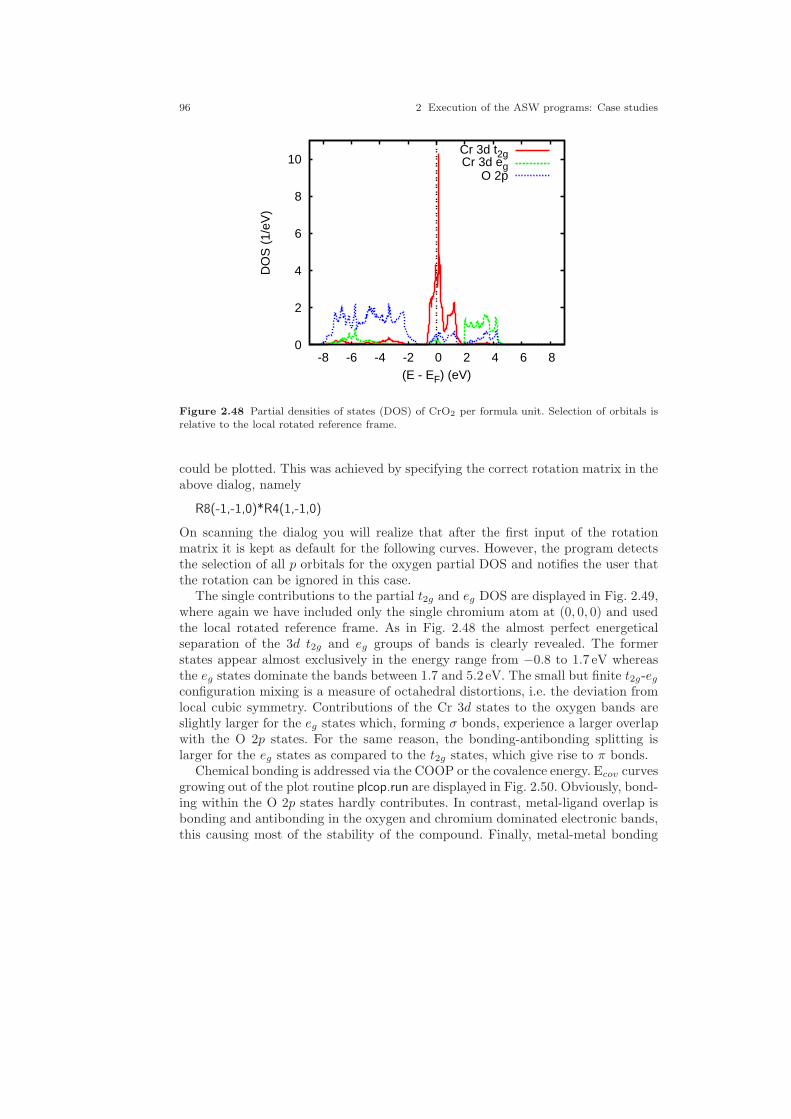
96 2 Execution of the ASW programs: Case studies
0
2
4
6
8
10
-8 -6 -4 -2 0 2 4 6 8
DO
S (
1/eV
)
(E - EF) (eV)
Cr 3d t2gCr 3d eg
O 2p
Figure 2.48 Partial densities of states (DOS) of CrO2 per formula unit. Selection of orbitals isrelative to the local rotated reference frame.
could be plotted. This was achieved by specifying the correct rotation matrix in theabove dialog, namely
R8(-1,-1,0)*R4(1,-1,0)
On scanning the dialog you will realize that after the first input of the rotationmatrix it is kept as default for the following curves. However, the program detectsthe selection of all p orbitals for the oxygen partial DOS and notifies the user thatthe rotation can be ignored in this case.
The single contributions to the partial t2g and eg DOS are displayed in Fig. 2.49,where again we have included only the single chromium atom at (0, 0, 0) and usedthe local rotated reference frame. As in Fig. 2.48 the almost perfect energeticalseparation of the 3d t2g and eg groups of bands is clearly revealed. The formerstates appear almost exclusively in the energy range from −0.8 to 1.7 eV whereasthe eg states dominate the bands between 1.7 and 5.2 eV. The small but finite t2g-eg
configuration mixing is a measure of octahedral distortions, i.e. the deviation fromlocal cubic symmetry. Contributions of the Cr 3d states to the oxygen bands areslightly larger for the eg states which, forming σ bonds, experience a larger overlapwith the O 2p states. For the same reason, the bonding-antibonding splitting islarger for the eg states as compared to the t2g states, which give rise to π bonds.
Chemical bonding is addressed via the COOP or the covalence energy. Ecov curvesgrowing out of the plot routine plcop.run are displayed in Fig. 2.50. Obviously, bond-ing within the O 2p states hardly contributes. In contrast, metal-ligand overlap isbonding and antibonding in the oxygen and chromium dominated electronic bands,this causing most of the stability of the compound. Finally, metal-metal bonding

2.4 A halfmetallic ferromagnet: CrO2 97
0
1
2
3
4
5
6
7
8
9
-2 -1 0 1 2 3 4 5 6
DO
S (
1/eV
)
(E - EF) (eV)
Cr 3dx2-y2
Cr 3dyzCr 3dxzCr 3dxy
Cr 3d3z2-r2
Figure 2.49 Partial Cr 3d t2g and eg densities of states (DOS) of CrO2. Selection of orbitals isrelative to the local rotated reference frame.
-1000
0
1000
2000
3000
-8 -6 -4 -2 0 2 4 6 8
EC
OV
(E - EF) (eV)
Cr 3d - Cr 3dO 2p - O 2pCr 3d - O 2p
Figure 2.50 Partial covalence energies (Ecov) of CrO2.
appears in the t2g and eg group of bands, being antibonding and bonding in therespective lower and upper part.
As has turned out in previous work on the neighbouring transition metal dioxidesinspection of the weighted band structures is a necessary prerequisite for a deeperunderstanding of these materials. This holds especially for the chromium 3d t2g
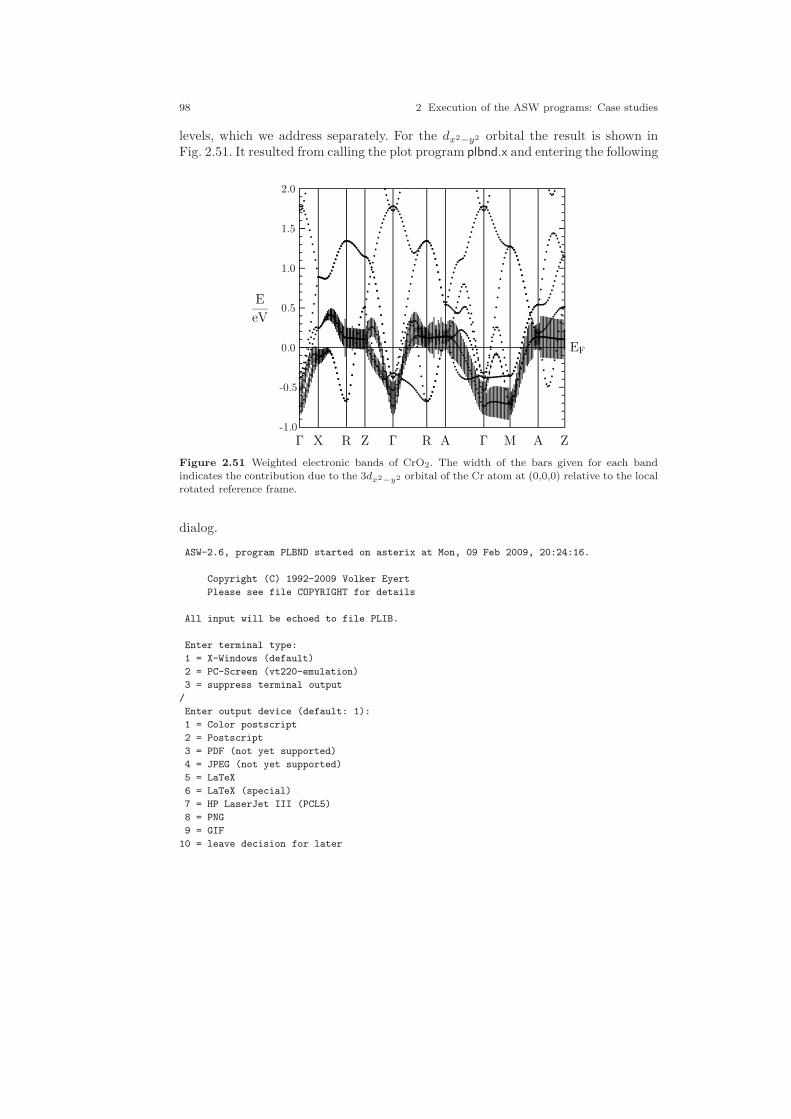
98 2 Execution of the ASW programs: Case studies
levels, which we address separately. For the dx2−y2 orbital the result is shown inFig. 2.51. It resulted from calling the plot program plbnd.x and entering the following
q
q
q
q
q
q
q
q
q
q
q
qqqqqqqqqq
q
q
q
q
q
q
q
q
q
q
qqq
q
q
q
q
q
q
qqqqqq
q
q
q
q
q
q
q
q
q
qqqq
q
q
q
q
qqq
q
q
q
q
qqqqqqqqqqqqqqqqqqqqqq
q
q
q
q
q
q
q
q
q
qqq
q
q
q
q
q
q
q
qqqqqqqqqqq
q
q
q
q
q
q
q
qqqqqqqqqqqqqqqqqqqqqq
q
q
q
q
q
q
q
q
q
q
q
q
q
qqqqqqqq
q
q
q
q
q
q
q
q
q
q
qqqqqq
q
q
q
q
q
q
qqqqqqqqqqqqqqq
q
q
q
q
q
q
q
q
q
q
qqq
q
q
q
q
q
q
qqqqqq
q
q
q
q
q
q
q
q
qqqqq
q
q
qqqqqq
q
q
q
q
q
q
q
q
q
q
q
qqqq
q
q
q
q
q
q
qqqq
q
q
q
q
q
q
q
q
q
qqqqqqqqqqqq
q
q
q
q
q
q
q
q
q
qqqqq
q
q
qqq
q
qqqqqqqqq
qqq
q
q
q
qqq
q
q
q
q
q
q
q
q
q
q
q
q
q
qqqqqqqqqqqqqqqqqqqqqqqqqq
qqq
q
q
q
q
q
q
q
q
q
q
qqqq
q
qqqqqqq
q
q
q
q
q
q
qqqqqqqqqqq
q
q
q
q
q
q
qqqqq
q
q
q
q
q
q
q
q
qqqqqqqqqqq
q
q
q
q
q
q
q
q
q
q
q
qqqqqqqqqqqqqqqqqqqqq
q
qqqqqq
qqqqqqqqqq
q
q
q
q
q
q
q
qqqqqqqq
q
q
q
q
qqq
q
q
q
q
qqqqqqq
q
q
q
q
q
q
q
q
q
q
q
q
q
q
q
q
qqq
qqqqqqqqqqqqqq
q
q
q
q
q
q
q
q
q
q
q
qqqqqqq
q
qqqqqqq
q
q
q
q
q
q
qqqqqqqqqqq
q
q
q
q
q
q
q
q
q
q
q
q
q
q
q
q
q
q
q
q
q
q
q
qqq
q
q
q
q
q
q
q
q
q
q
qqqqqqq
q
q
q
qqqqqqqqqqqq
qqqq
qqqq
q
q
q
qqqqqqqqqq
q
q
q
q
q
q
q
q
q
q
qqq
q
q
q
q
q
q
q
q
q
q
q
q
q
q
qqqq
q
q
q
q
q
q
q
q
q
q
q
q
q
q
q
q
qqqqqqqqqqqqqqqqqqqqqq
q
q
q
q
q
q
q
q
q
q
q
qqqqqqqqq
q
q
q
q
q
q
q
q
qqqqqqqq
qqqqqqqqqqqqq
q
q
q
q
q
q
q
q
q
q
q
q
q
q
q
qqqq
q
q
q
q
q
q
q
q
q
q
q
q
q
q
q
q
q
q
q
qqqqqqq
q
q
q
q
q
q
q
q
q
q
qqqqqqqq
q
q
q
q
q
q
q
q
q
q
q
q
q
q
q
q
q
qqq
q
q
q
q
q
q
q
q
q
q
q
q
q
q
q
qqqqqq
q
q
q
q
q
q
q
q
q
q
q
qqqqqqqqq
qqq
q
q
q
q
q
q
q
q
q
qqq
qqq
q
q
q
q
q
q
q
q
q
q
qqqqqqqqq
q
q
q
q
q
q
q
q
qqqqqqqq
qqqqqqqqqqqqq
q
q
q
q
q
q
q
q
q
q
q
q
q
qqqqqqqqq
q
q
q
q
q
q
q
q
q
qqqqqqqqqqqqqq
q
q
q
q
q
q
q
q
q
q
q
q
q
q
q
q
q
q
q
qqqqq
q
q
q
q
q
q
q
q
q
q
q
qqqqqqq
q
q
q
q
q
q
q
q
qqqqqqqqq
q
q
q
q
q
q
q
q
q
q
q
qqqqq
q
q
q
q
q
q
q
q
qqqqq
q
q
q
q
qqq
q
q
q
q
q
q
qqqqq
q
q
q
q
qqqqq
q
q
q
qqq
q
Γ X R Z Γ R A Γ M A Z
E
eV
EF
-1.0
-0.5
0.0
0.5
1.0
1.5
2.0
Figure 2.51 Weighted electronic bands of CrO2. The width of the bars given for each bandindicates the contribution due to the 3dx2
−y2 orbital of the Cr atom at (0,0,0) relative to the localrotated reference frame.
dialog.
ASW-2.6, program PLBND started on asterix at Mon, 09 Feb 2009, 20:24:16.
Copyright (C) 1992-2009 Volker Eyert
Please see file COPYRIGHT for details
All input will be echoed to file PLIB.
Enter terminal type:
1 = X-Windows (default)
2 = PC-Screen (vt220-emulation)
3 = suppress terminal output
/
Enter output device (default: 1):
1 = Color postscript
2 = Postscript
3 = PDF (not yet supported)
4 = JPEG (not yet supported)
5 = LaTeX
6 = LaTeX (special)
7 = HP LaserJet III (PCL5)
8 = PNG
9 = GIF
10 = leave decision for later

2.4 A halfmetallic ferromagnet: CrO2 99
11 = suppress output to file
6
Portrait (P, default) or landscape plot (L)?
/
Enter title:
Please wait a moment: I’m reading rest of file BNDE.
Timing for 19 points out of 194: 0.00000 sec.
Energies in Rydberg (F) or eV (T, default)?
/
Energies relative to MTZ (0) or EFermi (F, default)?
/
Energies connected by lines (T) (default F)?
/
Plot orbital character (default F)?
T
For plotting orbital character: Rotate reference frame for orbitals?
Enter rotation symbol (E for unity):
R8(-1,-1,0)*R4(1,-1,0)
Enter orbital(s) to be included:
Note: notation of the orbitals refers to the rotated reference frame!
Select from the classes (blank or "/" to complete the list):
CR O E1 E2 E3
CR
Class CR : atom 1 at 0.000000 0.000000 0.000000
Select from the following orbitals:
0: all -1: all p -2: all d
1: s 2: y 3: z 4: x 5: xy
6: yz 7: 3z^2-r^2 8: xz 9: x^2-y^2
9/
Class CR : atom 2 at -0.500000 -0.500000 -0.329790
Select from the following orbitals:
0: all -1: all p -2: all d
1: s 2: y 3: z 4: x 5: xy
6: yz 7: 3z^2-r^2 8: xz 9: x^2-y^2
/
Select from the classes (blank or "/" to complete the list):
CR O E1 E2 E3
/
The following orbitals have been selected:
Class CR : atom 1, orbital x^2-y^2
Ebot = -20.225934 eV , Etop = 83.109448 eV relative to EF
Emin = -21.000000 eV , Emax = 6.000000 eV relative to EF
Enter new Emin, Emax to change these defaults:
-1.0
2.0
Rescale orbital weights (default: 0.0750eV )?

100 2 Execution of the ASW programs: Case studies
0.3
Please wait a moment: I’m working on the weights.
Timing for 19 points out of 194: 0.01200 sec.
Enter the horizontal and vertical extension in mm.
Default: 100.0 x 90.0
/
task 1, total : cpu time: 0.25201 sec
ASW-2.6, program PLBND ended on asterix at Mon, 09 Feb 2009, 20:24:16.
Please delete files BNDE BNDV and bnd.tex when finished!!!
As in Sec. 2.1.4 the orbital to be included has to be specified. Here, the input“9” selects the dx2−y2 orbital. However, before the rotation matrix has to be givenin the same form as for program pldos.run above. Since LATEX output was requestedthe plot routine plbnd.run writes to the file bnd.tex, from which the postscript filebnd.ps is created by invoking the shell script plbnd.lx. The corresponding results forthe dxz and dyz orbitals are shown in Figs. 2.52 and 2.53. The following features
q
q
q
q
q
q
q
q
q
q
q
qqqqqqqqqq
q
q
q
q
q
q
q
q
q
q
qqq
q
q
q
q
q
q
qqqqqq
q
q
q
q
q
q
q
q
q
qqqq
q
q
q
q
qqq
q
q
q
q
qqqqqqqqqqqqqqqqqqqqqq
q
q
q
q
q
q
q
q
q
qqq
q
q
q
q
q
q
q
qqqqqqqqqqq
q
q
q
q
q
q
q
qqqqqqqqqqqqqqqqqqqqqq
q
q
q
q
q
q
q
q
q
q
q
q
q
qqqqqqqq
q
q
q
q
q
q
q
q
q
q
qqqqqq
q
q
q
q
q
q
qqqqqqqqqqqqqqq
q
q
q
q
q
q
q
q
q
q
qqq
q
q
q
q
q
q
qqqqqq
q
q
q
q
q
q
q
q
qqqqq
q
q
qqqqqq
q
q
q
q
q
q
q
q
q
q
q
qqqq
q
q
q
q
q
q
qqqq
q
q
q
q
q
q
q
q
q
qqqqqqqqqqqq
q
q
q
q
q
q
q
q
q
qqqqq
q
q
qqq
q
qqqqqqqqq
qqq
q
q
q
qqq
q
q
q
q
q
q
q
q
q
q
q
q
q
qqqqqqqqqqqqqqqqqqqqqqqqqq
qqq
q
q
q
q
q
q
q
q
q
q
qqqq
q
qqqqqqq
q
q
q
q
q
q
qqqqqqqqqqq
q
q
q
q
q
q
qqqqq
q
q
q
q
q
q
q
q
qqqqqqqqqqq
q
q
q
q
q
q
q
q
q
q
q
qqqqqqqqqqqqqqqqqqqqq
q
qqqqqq
qqqqqqqqqq
q
q
q
q
q
q
q
qqqqqqqq
q
q
q
q
qqq
q
q
q
q
qqqqqqq
q
q
q
q
q
q
q
q
q
q
q
q
q
q
q
q
qqq
qqqqqqqqqqqqqq
q
q
q
q
q
q
q
q
q
q
q
qqqqqqq
q
qqqqqqq
q
q
q
q
q
q
qqqqqqqqqqq
q
q
q
q
q
q
q
q
q
q
q
q
q
q
q
q
q
q
q
q
q
q
q
qqq
q
q
q
q
q
q
q
q
q
q
qqqqqqq
q
q
q
qqqqqqqqqqqq
qqqq
qqqq
q
q
q
qqqqqqqqqq
q
q
q
q
q
q
q
q
q
q
qqq
q
q
q
q
q
q
q
q
q
q
q
q
q
q
qqqq
q
q
q
q
q
q
q
q
q
q
q
q
q
q
q
q
qqqqqqqqqqqqqqqqqqqqqq
q
q
q
q
q
q
q
q
q
q
q
qqqqqqqqq
q
q
q
q
q
q
q
q
qqqqqqqq
qqqqqqqqqqqqq
q
q
q
q
q
q
q
q
q
q
q
q
q
q
q
qqqq
q
q
q
q
q
q
q
q
q
q
q
q
q
q
q
q
q
q
q
qqqqqqq
q
q
q
q
q
q
q
q
q
q
qqqqqqqq
q
q
q
q
q
q
q
q
q
q
q
q
q
q
q
q
q
qqq
q
q
q
q
q
q
q
q
q
q
q
q
q
q
q
qqqqqq
q
q
q
q
q
q
q
q
q
q
q
qqqqqqqqq
qqq
q
q
q
q
q
q
q
q
q
qqq
qqq
q
q
q
q
q
q
q
q
q
q
qqqqqqqqq
q
q
q
q
q
q
q
q
qqqqqqqq
qqqqqqqqqqqqq
q
q
q
q
q
q
q
q
q
q
q
q
q
qqqqqqqqq
q
q
q
q
q
q
q
q
q
qqqqqqqqqqqqqq
q
q
q
q
q
q
q
q
q
q
q
q
q
q
q
q
q
q
q
qqqqq
q
q
q
q
q
q
q
q
q
q
q
qqqqqqq
q
q
q
q
q
q
q
q
qqqqqqqqq
q
q
q
q
q
q
q
q
q
q
q
qqqqq
q
q
q
q
q
q
q
q
qqqqq
q
q
q
q
qqq
q
q
q
q
q
q
qqqqq
q
q
q
q
qqqqq
q
q
q
qqq
q
Γ X R Z Γ R A Γ M A Z
E
eV
EF
-1.0
-0.5
0.0
0.5
1.0
1.5
2.0
Figure 2.52 Weighted electronic bands of CrO2. The width of the bars given for each bandindicates the contribution due to the 3dxz orbital of the Cr atom at (0,0,0) relative to the localrotated reference frame.
are worth mentioning. On relating Fig. 2.51 to the Brillouin zone of the simpletetragonal lattice, Fig. B.5(a) we observe negligible dispersions along all lines withinthe planes spanned by the either the points Γ , X, and M, or else the points Z, R,and A. In contrast, dispersion along all lines connecting these plains is about 0.8 eV.

2.4 A halfmetallic ferromagnet: CrO2 101
q
q
q
q
q
q
q
q
q
q
q
qqqqqqqqqq
q
q
q
q
q
q
q
q
q
q
qqq
q
q
q
q
q
q
qqqqqq
q
q
q
q
q
q
q
q
q
qqqq
q
q
q
q
qqq
q
q
q
q
qqqqqqqqqqqqqqqqqqqqqq
q
q
q
q
q
q
q
q
q
qqq
q
q
q
q
q
q
q
qqqqqqqqqqq
q
q
q
q
q
q
q
qqqqqqqqqqqqqqqqqqqqqq
q
q
q
q
q
q
q
q
q
q
q
q
q
qqqqqqqq
q
q
q
q
q
q
q
q
q
q
qqqqqq
q
q
q
q
q
q
qqqqqqqqqqqqqqq
q
q
q
q
q
q
q
q
q
q
qqq
q
q
q
q
q
q
qqqqqq
q
q
q
q
q
q
q
q
qqqqq
q
q
qqqqqq
q
q
q
q
q
q
q
q
q
q
q
qqqq
q
q
q
q
q
q
qqqq
q
q
q
q
q
q
q
q
q
qqqqqqqqqqqq
q
q
q
q
q
q
q
q
q
qqqqq
q
q
qqq
q
qqqqqqqqq
qqq
q
q
q
qqq
q
q
q
q
q
q
q
q
q
q
q
q
q
qqqqqqqqqqqqqqqqqqqqqqqqqq
qqq
q
q
q
q
q
q
q
q
q
q
qqqq
q
qqqqqqq
q
q
q
q
q
q
qqqqqqqqqqq
q
q
q
q
q
q
qqqqq
q
q
q
q
q
q
q
q
qqqqqqqqqqq
q
q
q
q
q
q
q
q
q
q
q
qqqqqqqqqqqqqqqqqqqqq
q
qqqqqq
qqqqqqqqqq
q
q
q
q
q
q
q
qqqqqqqq
q
q
q
q
qqq
q
q
q
q
qqqqqqq
q
q
q
q
q
q
q
q
q
q
q
q
q
q
q
q
qqq
qqqqqqqqqqqqqq
q
q
q
q
q
q
q
q
q
q
q
qqqqqqq
q
qqqqqqq
q
q
q
q
q
q
qqqqqqqqqqq
q
q
q
q
q
q
q
q
q
q
q
q
q
q
q
q
q
q
q
q
q
q
q
qqq
q
q
q
q
q
q
q
q
q
q
qqqqqqq
q
q
q
qqqqqqqqqqqq
qqqq
qqqq
q
q
q
qqqqqqqqqq
q
q
q
q
q
q
q
q
q
q
qqq
q
q
q
q
q
q
q
q
q
q
q
q
q
q
qqqq
q
q
q
q
q
q
q
q
q
q
q
q
q
q
q
q
qqqqqqqqqqqqqqqqqqqqqq
q
q
q
q
q
q
q
q
q
q
q
qqqqqqqqq
q
q
q
q
q
q
q
q
qqqqqqqq
qqqqqqqqqqqqq
q
q
q
q
q
q
q
q
q
q
q
q
q
q
q
qqqq
q
q
q
q
q
q
q
q
q
q
q
q
q
q
q
q
q
q
q
qqqqqqq
q
q
q
q
q
q
q
q
q
q
qqqqqqqq
q
q
q
q
q
q
q
q
q
q
q
q
q
q
q
q
q
qqq
q
q
q
q
q
q
q
q
q
q
q
q
q
q
q
qqqqqq
q
q
q
q
q
q
q
q
q
q
q
qqqqqqqqq
qqq
q
q
q
q
q
q
q
q
q
qqq
qqq
q
q
q
q
q
q
q
q
q
q
qqqqqqqqq
q
q
q
q
q
q
q
q
qqqqqqqq
qqqqqqqqqqqqq
q
q
q
q
q
q
q
q
q
q
q
q
q
qqqqqqqqq
q
q
q
q
q
q
q
q
q
qqqqqqqqqqqqqq
q
q
q
q
q
q
q
q
q
q
q
q
q
q
q
q
q
q
q
qqqqq
q
q
q
q
q
q
q
q
q
q
q
qqqqqqq
q
q
q
q
q
q
q
q
qqqqqqqqq
q
q
q
q
q
q
q
q
q
q
q
qqqqq
q
q
q
q
q
q
q
q
qqqqq
q
q
q
q
qqq
q
q
q
q
q
q
qqqqq
q
q
q
q
qqqqq
q
q
q
qqq
q
Γ X R Z Γ R A Γ M A Z
E
eV
EF
-1.0
-0.5
0.0
0.5
1.0
1.5
2.0
Figure 2.53 Weighted electronic bands of CrO2. The width of the bars given for each bandindicates the contribution due to the 3dyz orbital of the Cr atom at (0,0,0) relative to the localrotated reference frame.
Thus one finds a predominantly one-dimensional behaviour. This is different for thebands highlighted in Figs. 2.52 and 2.53, which display dispersions of a similar sizealong all lines.
2.4.3 Spin-polarized ferromagnetic calculations
Before adapting the CTRL file for the spin-polarized calculations you should copyit to another directory (subdirectory fe already created before) in order to preservethe results of the non-magnetic calculations. In order to perform spin-polarizedcalculations two new tokens have to be added to the new CTRL file. In categoryOPTIONS the entry NSPIN=2 must be inserted, which tells the program to performa spin-polarized calculation. Furthermore, each orbital has to be given a startingvalue for the polarization. Otherwise the calculation would again converge to thespin-degenerate solution. Breaking the spin-symmetry is achieved by adding thetoken MVAL= for each atomic class in category CLASS followed by the polarizationfor each orbital. For ferromagnetic CrO2 the new categroy CLASS looks like thefollowing.
CLASS ATOM=CR Z=24 R=2.16612899 LMXL=2 CONF=4 4 3 4
QVAL= 1.0 0.0 5.0 0.0 MVAL= 0.0 0.0 2.0 0.0
ATOM=O Z= 8 R=1.87483912 LMXL=1 CONF=2 2 3
QVAL= 2.0 4.0 0.0 MVAL= 0.0 0.0 0.0
ATOM=E1 Z= 0 R=1.65252923 LMXL=1 CONF=1 2 3

102 2 Execution of the ASW programs: Case studies
QVAL= 0.0 0.0 0.0 MVAL= 0.0 0.0 0.0
ATOM=E2 Z= 0 R=1.76771917 LMXL=1 CONF=1 2 3
QVAL= 0.0 0.0 0.0 MVAL= 0.0 0.0 0.0
ATOM=E3 Z= 0 R=0.85735960 LMXL=0 CONF=1 2
QVAL= 0.0 0.0 MVAL= 0.0 0.0
Once these changes have been made you could type mnall.x as in the spin-degenerate case, Sec. 2.4.2. However, since you have only copied the CTRL fileto the new directory the program mnscf.run will start the spin-polarized calcula-tions from scratch. An alternative and very elegant way consists of also copyingthe atomic files of the converged non-magnetic calculations. Now invoking mnall.xlets the program mnscf.run (which is the first program called from the shell scriptmnall.x) detect the preconverged files. As already outlined in Sec. 2.1 this will invokethe restart facility of the program. During this startup phase the information fromthe converged spin-degenerate calculations is combined with the starting values forthe magnetic moments per orbital as given in the CTRL file in order to find anoptimal starting point for the spin-polarized calculation. As a consequence, veryfast iteration to full self-consistency is achieved.
After convergence monic outlst18 summarizes the results as follows.
ASW-2.6, program MNSCF started on asterix at Thu, 05 Feb 2009, 23:20:45.
Calculation converged after 14 iteration(s).
Start of Iteration 14
396 irreducible k-points generated from 4116 ( 14, 14, 21).
Fermi energy - MTZ = 0.739899 Ryd
The system is a magnetic metal and could still be a half-metallic ferromagnet:
DOS at Fermi energy: 18.932894 1/Ryd
Gamma * (f.u./cell): 3.280068 mJ/(mole*K**2)
Magnetic moment of unit cell = 4.000000
Mean-square residual: 0.681662D-23
Total free atom energies : -4790.190932 Ryd
Total variational energy : -4794.067509 Ryd
Cohesive energy : 3.876576 Ryd
qdiff = 0.00000000 < 0.00000001
ediff = 0.00000000 < 0.00000001
ASW-2.6, program MNSCF ended on asterix at Thu, 05 Feb 2009, 23:59:01.
According to this output a magnetic solution with a magnetic moment of 4.0µB
per unit cell has indeed been found. Its stability becomes obvious from a compar-ison of the total energy to that of the non-magnetic solution, the difference being72mRyd per formula unit. Worth mentioning is the considerable decrease of theDOS at EF as compared to the non-magnetic case. The reason is obvious from theband structure, Fig. 2.54, as well as in the corresponding density of states (DOS)as given in Fig. 2.55. While the O 2p-dominated spin-up and spin-down states stilloccupy similar energy intervals the Cr 3d bands experience spin-splitting of about2 eV. As a consequence, spin-minority Cr 3d states are shifted above the Fermienergy and left unoccupied. In contrast, metallic conductivity is carried alone bythe spin-majority states. The classification of CrO2 as a halfmetallic ferromagnetproposed by Schwarz is thus confirmed.
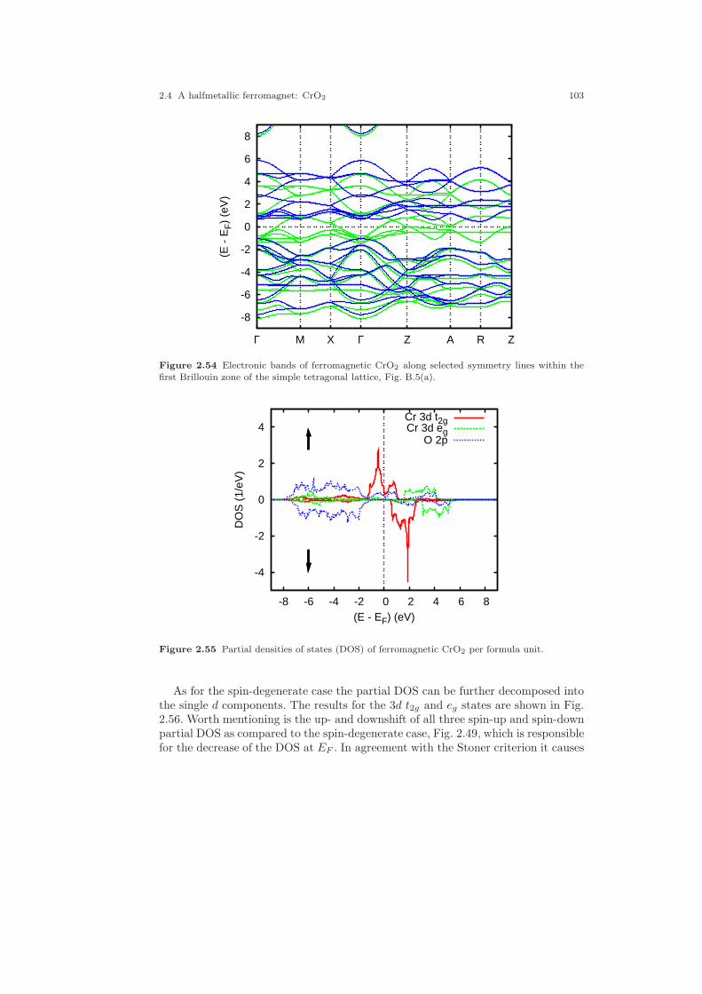
2.4 A halfmetallic ferromagnet: CrO2 103
-8
-6
-4
-2
0
2
4
6
8
Γ M X Γ Z A R Z
(E -
EF)
(eV
)
Figure 2.54 Electronic bands of ferromagnetic CrO2 along selected symmetry lines within thefirst Brillouin zone of the simple tetragonal lattice, Fig. B.5(a).
-4
-2
0
2
4
-8 -6 -4 -2 0 2 4 6 8
DO
S (
1/eV
)
(E - EF) (eV)
Cr 3d t2gCr 3d eg
O 2p
Figure 2.55 Partial densities of states (DOS) of ferromagnetic CrO2 per formula unit.
As for the spin-degenerate case the partial DOS can be further decomposed intothe single d components. The results for the 3d t2g and eg states are shown in Fig.2.56. Worth mentioning is the up- and downshift of all three spin-up and spin-downpartial DOS as compared to the spin-degenerate case, Fig. 2.49, which is responsiblefor the decrease of the DOS at EF . In agreement with the Stoner criterion it causes
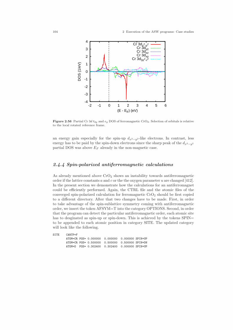
104 2 Execution of the ASW programs: Case studies
-4
-3
-2
-1
0
1
2
3
4
-2 -1 0 1 2 3 4 5 6
DO
S (
1/eV
)
(E - EF) (eV)
Cr 3dx2-y2
Cr 3dyzCr 3dxzCr 3dxy
Cr 3d3z2-r2
Figure 2.56 Partial Cr 3d t2g and eg DOS of ferromagnetic CrO2. Selection of orbitals is relativeto the local rotated reference frame.
an energy gain especially for the spin-up dx2−y2-like electrons. In contrast, lessenergy has to be paid by the spin-down electrons since the sharp peak of the dx2−y2
partial DOS was above EF already in the non-magnetic case.
2.4.4 Spin-polarized antiferromagnetic calculations
As already mentioned above CrO2 shows an instability towards antiferromagneticorder if the lattice constants a and c or the the oxygen parameter u are changed [412].In the present section we demonstrate how the calculations for an antiferromagnetcould be efficiently performed. Again, the CTRL file and the atomic files of theconverged spin-polarized calculation for ferromagnetic CrO2 should be first copiedto a different directory. After that two changes have to be made. First, in orderto take advantage of the spin-sublattice symmetry coming with antiferromagneticorder, we insert the token AFSYM=T into the category OPTIONS. Second, in orderthat the program can detect the particular antiferromagnetic order, each atomic sitehas to desginated as spin-up or spin-down. This is achieved by the tokens SPIN=to be appended to each atomic position in category SITE. The updated categorywill look like the following.
SITE CARTP=F
ATOM=CR POS= 0.000000 0.000000 0.000000 SPIN=UP
ATOM=CR POS= 0.500000 0.500000 0.500000 SPIN=DN
ATOM=O POS= 0.302400 0.302400 0.000000 SPIN=UP

2.4 A halfmetallic ferromagnet: CrO2 105
ATOM=O POS=-0.302400 -0.302400 0.000000 SPIN=UP
ATOM=O POS=-0.197600 0.197600 0.500000 SPIN=DN
ATOM=O POS= 0.197600 -0.197600 0.500000 SPIN=DN
ATOM=E1 POS= 0.500000 0.000000 -0.250000 SPIN=DN
ATOM=E1 POS= 0.500000 0.000000 0.250000 SPIN=UP
ATOM=E1 POS= 0.000000 -0.500000 -0.250000 SPIN=DN
ATOM=E1 POS= 0.000000 -0.500000 0.250000 SPIN=UP
ATOM=E2 POS= 0.318691 -0.318691 0.000000 SPIN=UP
ATOM=E2 POS=-0.318691 0.318691 0.000000 SPIN=UP
ATOM=E2 POS=-0.181309 -0.181309 -0.500000 SPIN=DN
ATOM=E2 POS= 0.181309 0.181309 -0.500000 SPIN=DN
ATOM=E3 POS= 0.313120 -0.055474 0.000000 SPIN=UP
ATOM=E3 POS=-0.313120 0.055474 0.000000 SPIN=UP
ATOM=E3 POS=-0.186880 -0.444526 -0.500000 SPIN=DN
ATOM=E3 POS= 0.186880 0.444526 0.500000 SPIN=DN
ATOM=E3 POS= 0.055474 -0.313120 0.000000 SPIN=UP
ATOM=E3 POS=-0.055474 0.313120 0.000000 SPIN=UP
ATOM=E3 POS=-0.444526 -0.186880 -0.500000 SPIN=DN
ATOM=E3 POS= 0.444526 0.186880 -0.500000 SPIN=DN
Note that for each class there must be an equal number of SPIN=UP andSPIN=DN entries. Again the self-consistent calculation is started by typing mnall.xat the systems prompt. In case you have forgotten to copy the atomic files of theferromagnetic calculation the program will start from scratch and, hence, need moreiterations. Of course, for antiferromagnetic materials it is not not necessary to per-form a ferromagnetic calculation first. You could also use the atomic files of aspin-degenerate calculation as a starting point for an antiferromagnetic calculation.
After convergence monic outlst18 summarizes the results as follows.
ASW-2.6, program MNSCF started on asterix at Thu, 05 Feb 2009, 23:43:25.
Calculation converged after 18 iteration(s).
Start of Iteration 18
756 irreducible k-points generated from 4116 ( 14, 14, 21).
Fermi energy - MTZ = 0.732169 Ryd
The system is a magnetic metal and could still be a half-metallic ferromagnet:
DOS at Fermi energy: 61.416030 1/Ryd
Gamma * (f.u./cell): 10.640147 mJ/(mole*K**2)
Magnetic moment of UP atoms = 1.703860
Magnetic moment of unit cell = 0.000000
Mean-square residual: 0.552659D-23
Total free atom energies : -4790.190932 Ryd
Total variational energy : -4794.045025 Ryd
Cohesive energy : 3.854093 Ryd
qdiff = 0.00000000 < 0.00000001
ediff = 0.00000000 < 0.00000001
ASW-2.6, program MNSCF ended on asterix at Fri, 06 Feb 2009, 00:34:18.
According to this output a magnetic solution with a magnetic moment of ≈ 1.7µB
per sublattice has indeed been found. However, while being stable as compared tothe spin-degenerate case, its total energy is by 22mRyd per formula higher as thatof the ferromagnetic solution.
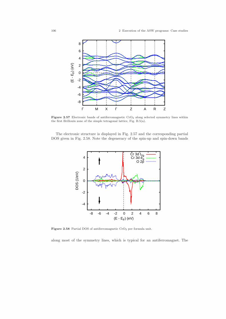
106 2 Execution of the ASW programs: Case studies
-8
-6
-4
-2
0
2
4
6
8
Γ M X Γ Z A R Z
(E -
EF)
(eV
)
Figure 2.57 Electronic bands of antiferromagnetic CrO2 along selected symmetry lines withinthe first Brillouin zone of the simple tetragonal lattice, Fig. B.5(a).
The electronic structure is displayed in Fig. 2.57 and the corresponding partialDOS given in Fig. 2.58. Note the degeneracy of the spin-up and spin-down bands
-4
-2
0
2
4
-8 -6 -4 -2 0 2 4 6 8
DO
S (
1/eV
)
(E - EF) (eV)
Cr 3d t2gCr 3d eg
O 2p
Figure 2.58 Partial DOS of antiferromagnetic CrO2 per formula unit.
along most of the symmetry lines, which is typical for an antiferromagnet. The
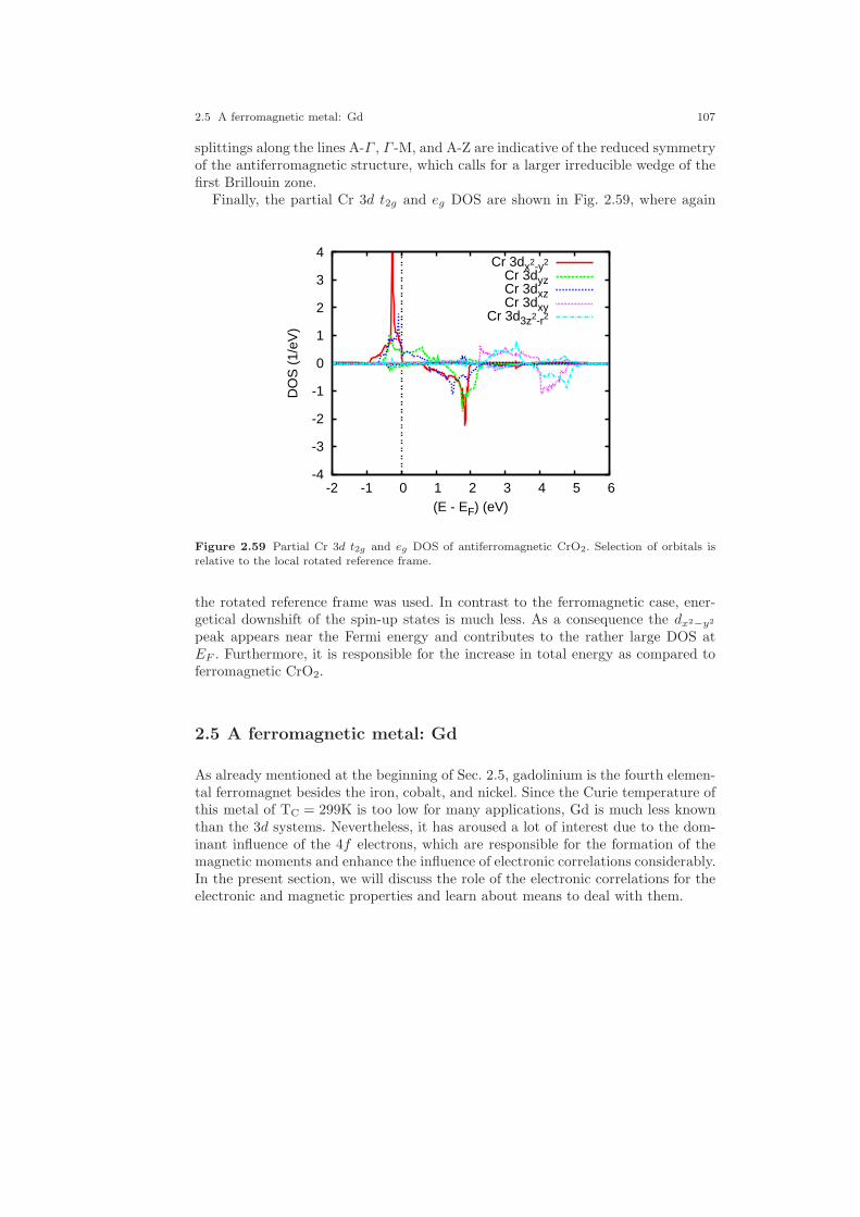
2.5 A ferromagnetic metal: Gd 107
splittings along the lines A-Γ , Γ -M, and A-Z are indicative of the reduced symmetryof the antiferromagnetic structure, which calls for a larger irreducible wedge of thefirst Brillouin zone.
Finally, the partial Cr 3d t2g and eg DOS are shown in Fig. 2.59, where again
-4
-3
-2
-1
0
1
2
3
4
-2 -1 0 1 2 3 4 5 6
DO
S (
1/eV
)
(E - EF) (eV)
Cr 3dx2-y2
Cr 3dyzCr 3dxzCr 3dxy
Cr 3d3z2-r2
Figure 2.59 Partial Cr 3d t2g and eg DOS of antiferromagnetic CrO2. Selection of orbitals isrelative to the local rotated reference frame.
the rotated reference frame was used. In contrast to the ferromagnetic case, ener-getical downshift of the spin-up states is much less. As a consequence the dx2−y2
peak appears near the Fermi energy and contributes to the rather large DOS atEF . Furthermore, it is responsible for the increase in total energy as compared toferromagnetic CrO2.
2.5 A ferromagnetic metal: Gd
As already mentioned at the beginning of Sec. 2.5, gadolinium is the fourth elemen-tal ferromagnet besides the iron, cobalt, and nickel. Since the Curie temperature ofthis metal of TC = 299K is too low for many applications, Gd is much less knownthan the 3d systems. Nevertheless, it has aroused a lot of interest due to the dom-inant influence of the 4f electrons, which are responsible for the formation of themagnetic moments and enhance the influence of electronic correlations considerably.In the present section, we will discuss the role of the electronic correlations for theelectronic and magnetic properties and learn about means to deal with them.
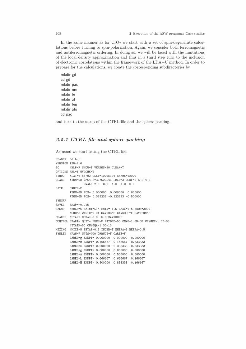
108 2 Execution of the ASW programs: Case studies
In the same manner as for CrO2 we start with a set of spin-degenerate calcu-lations before turning to spin-polarization. Again, we consider both ferromagneticand antiferromagnetic ordering. In doing so, we will be faced with the limitationsof the local density approximation and thus in a third step turn to the inclusionof electronic correlations within the framework of the LDA+U method. In order toprepare for the calculations, we create the corresponding subdirectories by
mkdir gdcd gdmkdir pacmkdir nmmkdir femkdir afmkdir feumkdir afucd pac
and turn to the setup of the CTRL file and the sphere packing.
2.5.1 CTRL file and sphere packing
As usual we start listing the CTRL file.
HEADER Gd hcp
VERSION ASW-2.6
IO HELP=F SHOW=T VERBOS=30 CLEAN=T
OPTIONS REL=T OVLCHK=T
STRUC ALAT=6.85782 CLAT=10.95194 GAMMA=120.0
CLASS ATOM=GD Z=64 R=3.7620545 LMXL=3 CONF=6 6 5 4 5
QVAL= 2.0 0.0 1.0 7.0 0.0
SITE CARTP=F
ATOM=GD POS= 0.000000 0.000000 0.000000
ATOM=GD POS= 0.333333 -0.333333 -0.500000
SYMGRP
ENVEL EKAP=-0.015
BZSMP NKBAB=6 BZINT=LTM EMIN=-1.5 EMAX=1.5 NDOS=3000
NORD=3 WIDTH=0.01 SAVDOS=F SAVCOOP=F SAVFERM=F
CHARGE NETA=2 EETA=-3.0 -5.0 SAVRHO=F
CONTROL START= QUIT= FREE=F NITBND=50 CNVG=1.0D-08 CNVGET=1.0D-08
NITATM=50 CNVGQA=1.0D-10
MIXING NMIXB=5 BETAB=0.5 INCBB=T NMIXA=5 BETAA=0.5
SYMLIN NPAN=7 NPTS=400 ORBWGT=F CARTE=F
LABEL=g ENDPT= 0.000000 0.000000 0.000000
LABEL=M ENDPT= 0.166667 0.166667 -0.333333
LABEL=K ENDPT= 0.000000 0.333333 -0.333333
LABEL=g ENDPT= 0.000000 0.000000 0.000000
LABEL=A ENDPT= 0.500000 0.500000 0.500000
LABEL=L ENDPT= 0.666667 0.666667 0.166667
LABEL=H ENDPT= 0.500000 0.833333 0.166667

2.5 A ferromagnetic metal: Gd 109
LABEL=A ENDPT= 0.500000 0.500000 0.500000
PLOT CARTV=F
ORIGIN= 0.65 0.35 0.0
RPLOT1=-1.0 1.0 0.0
RPLOT2= 0.0 0.0 1.0
RPLOT3= 1.0 1.0 0.0
NPDIV1=50 NPDIV2=50 NPDIV3=0
PLOT CARTV=F
ORIGIN= 0.0 0.0 0.0
RPLOT1= 1.0 0.0 0.0
RPLOT2= 0.0 1.0 0.0
RPLOT3= 0.0 0.0 1.0
NPDIV1=50 NPDIV2=50 NPDIV3=0
A few tokens are of interest here. In category STRUC and so far not used tokenenters, namely GAMMA=, which reflects the 120◦ angle between the basal planeprimitive translations of the hexagonal lattice adopted by Gd. In addition, as for thetetragonal lattice of CrO2, we specified the c lattice constant by the token CLAT=.Finally, note the entries in category SYMLIN=, where we have specified the endpoints usually applied for the hexagonal lattice. Whenever you are in doubt aboutthe specification of the end points remove this category from the CTRL file and theprograms will propose a standard setting for the particular lattice.
As before, we start running the packing routine mnpac.x, which returns the mes-sage that all volume can be filled without empty spheres and with a linear overlap ofonly 11%. Of course, this is a consequence of the hexagonal close packed structure.
2.5.2 Spin-degenerate calculations
We are thus able to start with the spin-degenerate set of calculatons rightaway byentering
mnall.x
at the systems prompt. As already mentioned, we prefer starting with the non-magnetic case in order to have a reference at hand. Moreover, we will benefit fromthe restart facility of the ASW program mnscf.run.
After convergence has been achieved the command monic outlst18 collects themost important results.
ASW-2.6, program MNSCF started on asterix at Thu, 05 Feb 2009, 13:03:41.
Calculation converged after 25 iteration(s).
Start of Iteration 25
240 irreducible k-points generated from 3610 ( 19, 19, 10).
Fermi energy - MTZ = 0.457108 Ryd
The system is a metal:
DOS at Fermi energy: 1256.643248 1/Ryd
Gamma * (f.u./cell): 217.709763 mJ/(mole*K**2)
Mean-square residual: 0.229578D-22
Total free atom energies : -45054.284175 Ryd

110 2 Execution of the ASW programs: Case studies
Total variational energy : -45055.309795 Ryd
Cohesive energy : 1.025620 Ryd
qdiff = 0.00000000 < 0.00000001
ediff = 0.00000000 < 0.00000001
ASW-2.6, program MNSCF ended on asterix at Thu, 05 Feb 2009, 13:06:10.
As a matter of fact, non-magnetic Gd is a metal with a huge density of statesat EF . Hence, from Stoner theory we would expect ferromagnetic ordering. Wedisplay in Fig. 2.60 the electronic states along selected high symmetry lines within
-6
-4
-2
0
2
4
6
Γ M K Γ A L H A
(E -
EF)
(eV
)
Figure 2.60 Electronic bands of Gd along selected symmetry lines within the first Brillouin zoneof the hexagonal lattice, Fig. B.4.
the first Brillouin zone of the hexagonal lattice, Fig. B.4. The corresponding densityof states (DOS) is given in Fig. 2.61. From Figs. 2.60 and 2.61 the interpretationof the results is rather simple. While the electronic states are dominated by thesharp 4f peak at EF , the d states show a rather large dispersion eveolving from aparabolic band at the Γ point.
2.5.3 Spin-polarized calculations
Turning to the spin-polarized calculations we begin copying the CTRL file as wellas the atomic file GD to the subdirectories fe and af for use as a starting point. Still,a few things have to be changed in the CTRL files. First, in category OPTIONSthe entry NSPIN=2 must be inserted, which tells the program to perform a spin-
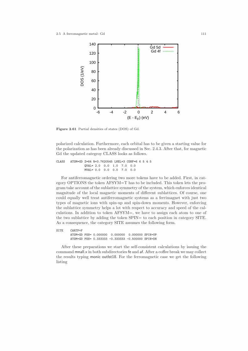
2.5 A ferromagnetic metal: Gd 111
0
20
40
60
80
100
120
140
-6 -4 -2 0 2 4 6
DO
S (
1/eV
)
(E - EF) (eV)
Gd 5dGd 4f
Figure 2.61 Partial densities of states (DOS) of Gd.
polarized calculation. Furthermore, each orbital has to be given a starting value forthe polarization as has been already discussed in Sec. 2.4.3. After that, for magneticGd the updated categroy CLASS looks as follows.
CLASS ATOM=GD Z=64 R=3.7620545 LMXL=3 CONF=6 6 5 4 5
QVAL= 2.0 0.0 1.0 7.0 0.0
MVAL= 0.0 0.0 0.0 7.0 0.0
For antiferromagnetic ordering two more tokens have to be added. First, in cat-egory OPTIONS the token AFSYM=T has to be included. This token lets the pro-gram take account of the sublattice symmetry of the system, which enforces identicalmagnitude of the local magnetic moments of different sublattices. Of course, onecould equally well treat antiferromagnetic systems as a ferrimagnet with just twotypes of magnetic ions with spin-up and spin-down moments. However, enforcingthe sublattice symmetry helps a lot with respect to accuracy and speed of the cal-culations. In addition to token AFSYM=, we have to assign each atom to one ofthe two sublattice by adding the token SPIN= to each position in category SITE.As a consequence, the category SITE assumes the following form.
SITE CARTP=F
ATOM=GD POS= 0.000000 0.000000 0.000000 SPIN=UP
ATOM=GD POS= 0.333333 -0.333333 -0.500000 SPIN=DN
After these preparations we start the self-consistent calculations by issuing thecommand mnall.x in both subdirectories fe and af. After a coffee break we may collectthe results typing monic outlst18. For the ferromagnetic case we get the followinglisting
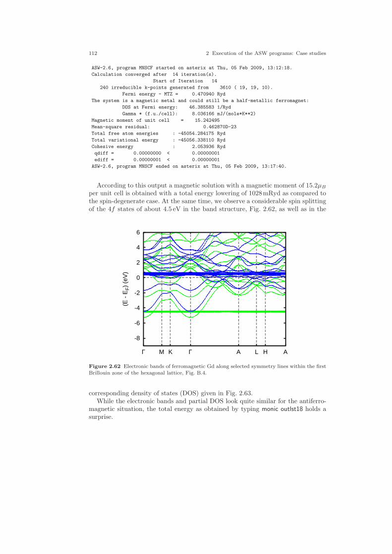
112 2 Execution of the ASW programs: Case studies
ASW-2.6, program MNSCF started on asterix at Thu, 05 Feb 2009, 13:12:18.
Calculation converged after 14 iteration(s).
Start of Iteration 14
240 irreducible k-points generated from 3610 ( 19, 19, 10).
Fermi energy - MTZ = 0.470940 Ryd
The system is a magnetic metal and could still be a half-metallic ferromagnet:
DOS at Fermi energy: 46.385583 1/Ryd
Gamma * (f.u./cell): 8.036166 mJ/(mole*K**2)
Magnetic moment of unit cell = 15.242495
Mean-square residual: 0.462870D-23
Total free atom energies : -45054.284175 Ryd
Total variational energy : -45056.338110 Ryd
Cohesive energy : 2.053936 Ryd
qdiff = 0.00000000 < 0.00000001
ediff = 0.00000001 < 0.00000001
ASW-2.6, program MNSCF ended on asterix at Thu, 05 Feb 2009, 13:17:40.
According to this output a magnetic solution with a magnetic moment of 15.2µB
per unit cell is obtained with a total energy lowering of 1028mRyd as compared tothe spin-degenerate case. At the same time, we observe a considerable spin splittingof the 4f states of about 4.5 eV in the band structure, Fig. 2.62, as well as in the
-8
-6
-4
-2
0
2
4
6
Γ M K Γ A L H A
(E -
EF)
(eV
)
Figure 2.62 Electronic bands of ferromagnetic Gd along selected symmetry lines within the firstBrillouin zone of the hexagonal lattice, Fig. B.4.
corresponding density of states (DOS) given in Fig. 2.63.While the electronic bands and partial DOS look quite similar for the antiferro-
magnetic situation, the total energy as obtained by typing monic outlst18 holds asurprise.

2.5 A ferromagnetic metal: Gd 113
-100
-50
0
50
100
-8 -6 -4 -2 0 2 4 6
DO
S (
1/eV
)
(E - EF) (eV)
Gd 5dGd 4f
Figure 2.63 Partial densities of states (DOS) of ferromagnetic Gd.
ASW-2.6, program MNSCF started on asterix at Thu, 05 Feb 2009, 13:14:34.
Calculation converged after 14 iteration(s).
Start of Iteration 14
240 irreducible k-points generated from 3610 ( 19, 19, 10).
Fermi energy - MTZ = 0.471016 Ryd
The system is a magnetic metal:
DOS at Fermi energy: 42.067504 1/Ryd
Gamma * (f.u./cell): 7.288072 mJ/(mole*K**2)
Magnetic moment of UP atoms = 7.366000
Magnetic moment of unit cell = 0.000000
Mean-square residual: 0.774390D-24
Total free atom energies : -45054.284175 Ryd
Total variational energy : -45056.341314 Ryd
Cohesive energy : 2.057140 Ryd
qdiff = 0.00000000 < 0.00000001
ediff = 0.00000000 < 0.00000001
ASW-2.6, program MNSCF ended on asterix at Thu, 05 Feb 2009, 13:19:00.
According to the output, antiferromagnetically ordered gadoliniom is still morestable than the ferromagnet by 3.2mRyd. This is in striking contrast to experimentand can be traced back to the limitations of the local density approximation.
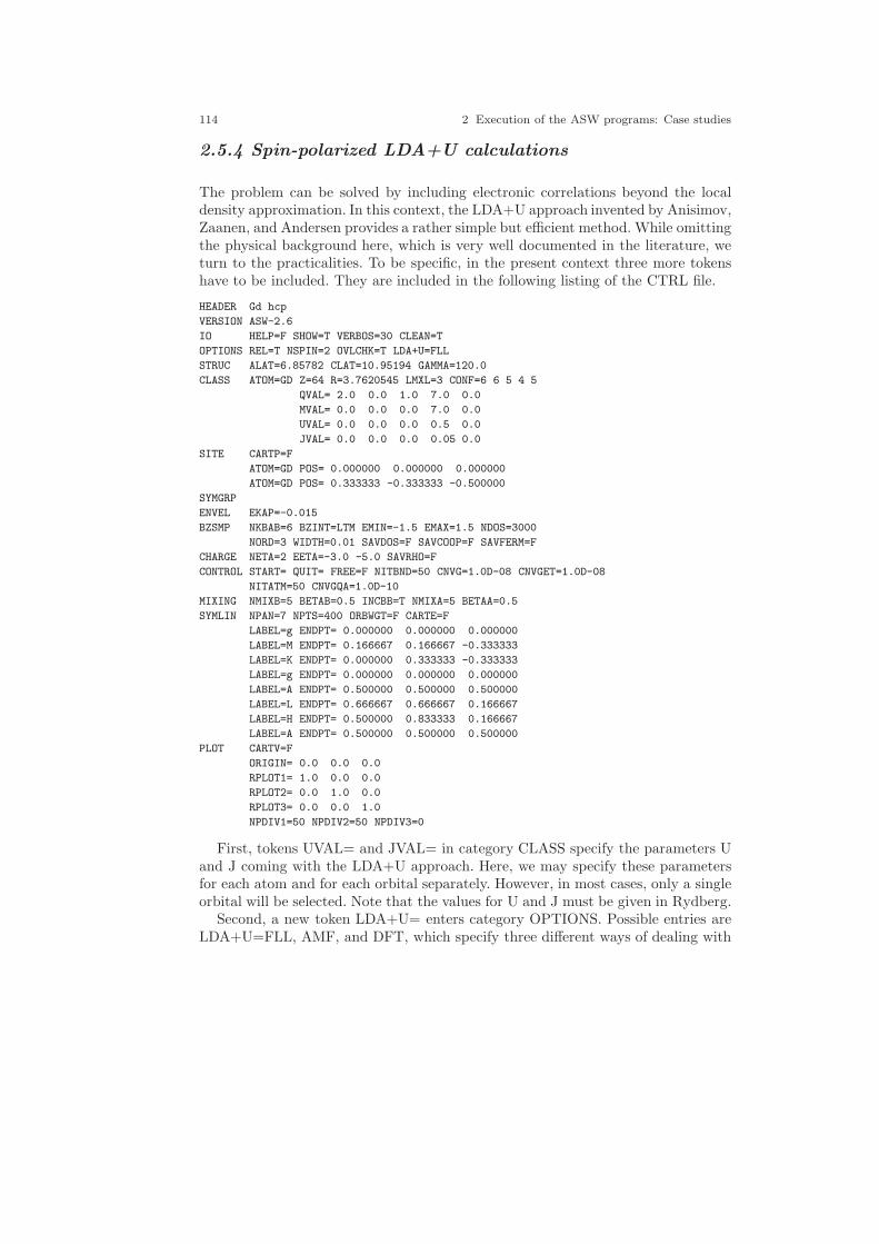
114 2 Execution of the ASW programs: Case studies
2.5.4 Spin-polarized LDA+U calculations
The problem can be solved by including electronic correlations beyond the localdensity approximation. In this context, the LDA+U approach invented by Anisimov,Zaanen, and Andersen provides a rather simple but efficient method. While omittingthe physical background here, which is very well documented in the literature, weturn to the practicalities. To be specific, in the present context three more tokenshave to be included. They are included in the following listing of the CTRL file.
HEADER Gd hcp
VERSION ASW-2.6
IO HELP=F SHOW=T VERBOS=30 CLEAN=T
OPTIONS REL=T NSPIN=2 OVLCHK=T LDA+U=FLL
STRUC ALAT=6.85782 CLAT=10.95194 GAMMA=120.0
CLASS ATOM=GD Z=64 R=3.7620545 LMXL=3 CONF=6 6 5 4 5
QVAL= 2.0 0.0 1.0 7.0 0.0
MVAL= 0.0 0.0 0.0 7.0 0.0
UVAL= 0.0 0.0 0.0 0.5 0.0
JVAL= 0.0 0.0 0.0 0.05 0.0
SITE CARTP=F
ATOM=GD POS= 0.000000 0.000000 0.000000
ATOM=GD POS= 0.333333 -0.333333 -0.500000
SYMGRP
ENVEL EKAP=-0.015
BZSMP NKBAB=6 BZINT=LTM EMIN=-1.5 EMAX=1.5 NDOS=3000
NORD=3 WIDTH=0.01 SAVDOS=F SAVCOOP=F SAVFERM=F
CHARGE NETA=2 EETA=-3.0 -5.0 SAVRHO=F
CONTROL START= QUIT= FREE=F NITBND=50 CNVG=1.0D-08 CNVGET=1.0D-08
NITATM=50 CNVGQA=1.0D-10
MIXING NMIXB=5 BETAB=0.5 INCBB=T NMIXA=5 BETAA=0.5
SYMLIN NPAN=7 NPTS=400 ORBWGT=F CARTE=F
LABEL=g ENDPT= 0.000000 0.000000 0.000000
LABEL=M ENDPT= 0.166667 0.166667 -0.333333
LABEL=K ENDPT= 0.000000 0.333333 -0.333333
LABEL=g ENDPT= 0.000000 0.000000 0.000000
LABEL=A ENDPT= 0.500000 0.500000 0.500000
LABEL=L ENDPT= 0.666667 0.666667 0.166667
LABEL=H ENDPT= 0.500000 0.833333 0.166667
LABEL=A ENDPT= 0.500000 0.500000 0.500000
PLOT CARTV=F
ORIGIN= 0.0 0.0 0.0
RPLOT1= 1.0 0.0 0.0
RPLOT2= 0.0 1.0 0.0
RPLOT3= 0.0 0.0 1.0
NPDIV1=50 NPDIV2=50 NPDIV3=0
First, tokens UVAL= and JVAL= in category CLASS specify the parameters Uand J coming with the LDA+U approach. Here, we may specify these parametersfor each atom and for each orbital separately. However, in most cases, only a singleorbital will be selected. Note that the values for U and J must be given in Rydberg.
Second, a new token LDA+U= enters category OPTIONS. Possible entries areLDA+U=FLL, AMF, and DFT, which specify three different ways of dealing with

2.5 A ferromagnetic metal: Gd 115
the so-called double counting terms. Actually, for systems, which are only weaklycorrelated, the choice of the double-counting correction can be rather sensitive tothe results. However, for strongly correlated systems as Gd the fully localized limit(FLL) is a good choice.
Having included these specifications in the CTRL files for both the ferromagneticand antiferromagnetic situation (after having copyied them to the subdirectories feuand afu and after having also copied the file GD to these directories) we start thestandard canon of calculations again, which allows us to take another coffee break.
After successful completion of the calculations the results are summarized in thelistings
ASW-2.6, program MNSCF started on asterix at Thu, 05 Feb 2009, 13:38:56.
Calculation converged after 13 iteration(s).
Start of Iteration 13
240 irreducible k-points generated from 3610 ( 19, 19, 10).
Fermi energy - MTZ = 0.472938 Ryd
The system is a magnetic metal:
DOS at Fermi energy: 25.238563 1/Ryd
Gamma * (f.u./cell): 4.372507 mJ/(mole*K**2)
Magnetic moment of unit cell = 15.670950
Mean-square residual: 0.161670D-22
Total free atom energies : -45054.284175 Ryd
Total variational energy : -45056.340574 Ryd
Cohesive energy : 2.056400 Ryd
qdiff = 0.00000000 < 0.00000001
ediff = 0.00000001 < 0.00000001
ASW-2.6, program MNSCF ended on asterix at Thu, 05 Feb 2009, 13:46:38.
for the ferromagnet and
ASW-2.6, program MNSCF started on asterix at Thu, 05 Feb 2009, 13:40:24.
Calculation converged after 12 iteration(s).
Start of Iteration 12
240 irreducible k-points generated from 3610 ( 19, 19, 10).
Fermi energy - MTZ = 0.471700 Ryd
The system is a magnetic metal and could still be a half-metallic ferromagnet:
DOS at Fermi energy: 36.055204 1/Ryd
Gamma * (f.u./cell): 6.246459 mJ/(mole*K**2)
Magnetic moment of UP atoms = 7.502246
Magnetic moment of unit cell = 0.000000
Mean-square residual: 0.248595D-22
Total free atom energies : -45054.284175 Ryd
Total variational energy : -45056.323725 Ryd
Cohesive energy : 2.039550 Ryd
qdiff = 0.00000000 < 0.00000001
ediff = 0.00000000 < 0.00000001
ASW-2.6, program MNSCF ended on asterix at Thu, 05 Feb 2009, 13:47:08.
for the antiferromagnet. Obviously, the order of the total energies is reversed andwe obtain a ferromegnatic ground state in agreement with experiment. At the sametime, the magnetic moment per cell has slightly increased. Striking changes are also
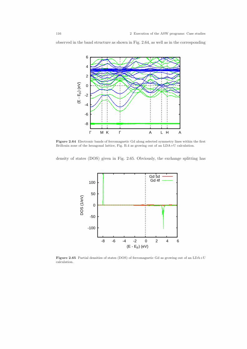
116 2 Execution of the ASW programs: Case studies
observed in the band structure as shown in Fig. 2.64, as well as in the corresponding
-8
-6
-4
-2
0
2
4
6
Γ M K Γ A L H A
(E -
EF)
(eV
)
Figure 2.64 Electronic bands of ferromagnetic Gd along selected symmetry lines within the firstBrillouin zone of the hexagonal lattice, Fig. B.4 as growing out of an LDA+U calculation.
density of states (DOS) given in Fig. 2.65. Obviously, the exchange splitting has
-100
-50
0
50
100
-8 -6 -4 -2 0 2 4 6
DO
S (
1/eV
)
(E - EF) (eV)
Gd 5dGd 4f
Figure 2.65 Partial densities of states (DOS) of ferromagnetic Gd as growing out of an LDA+Ucalculation.

2.5 A ferromagnetic metal: Gd 117
considerably increased to a value of about 11.5 eV due to the localizing nature ofthe LDA+U approach. Again, this is in much better agreement with experimentaldata from photoemission studies.


Chapter 3
Organization of the ASW programpackage
In the present chapter an overview is given over all files coming with the distributionor being generated during the execution of the programs. This includes mainly fourgroups. While the calculations are performed by one of the main programs, theplot programs serve the purpose of visualizing the results. Work of both steps ismade easier by a number of shell scripts. Finally, a list of all files, which are eitherincluded in the distribution or else created by one of the programs, is given.
3.1 Main programs and shell scripts
In the present section all main programs of the ASW distribution are discussed. Incontrast to the plot programs presented in the following section, all main programs(with the exception of mnmpr.run) start reading the CTRL file.
As has been already outlined in Sec. 2.1, the ASW program package includesboth the executables (with ending “.run”) and corresponding shell scripts (withending “.x”). The latter call the executables and specify the respective output files.In addition, the shell scripts provide commands for the most common job queuingsystems as IBM’s LoadLeveler (LoadL), and the public domain packages PortableBatch System (PBS) and Sun’s Grid Engine (SGE) (support for the Network Queu-ing System (NQS) and the Distributed Queuing System (DQS) is also included butthese systems do not seem to be used any more). Finally, some of the shell scriptsinclude appropriate modifications of the CTRL file. A fully commented exampleshell script is contained in the file mnhlp.x, which should be consulted for moreinformation. In the following discussion we will use the names program, executableand shell script synonymously.
119

120 3 Organization of the ASW program package
3.1.1 mnmpr.run, mnmpr.x
While all main programs calculate the parameters of the actual machine at the verybeginning, this program prints them out and stops. The output usually looks likefile MACHi coming with the distribution.
ASW-2.6, program MNMPR started on asterix at Thu, 15 Jan 2009, 11:47:11.
Copyright (C) 1992-2009 Volker Eyert
Please see file COPYRIGHT for details
Machine-specific parameters affecting floating-point arithmethic:
ibase: 2 (base of the machine)
it: 53 (number of (base) digits in the mantissa)
xeps: 2.22044604925031D-16 (= min, such that 1.0 + xeps > 1.0)
xepsn: 1.11022302462516D-16 (= min, such that 1.0 - xepsn < 1.0)
minexp: -1021 (min exponent before (gradual) underflow)
xzer: 2.22507385850720-308 (underflow threshold = base**(minexp-1))
xmin: 2.22507385850720-308 (safe min, 1/xmin does not overflow)
maxexp: 1024 (largest exponent before overflow)
xinf: 1.79769313486232+308 (overflow threshold = base**maxexp*(1-xepsn))
irnd: 1 (= 0/1 for chopping/rounding in addition)
task 1, total : cpu time: 0.00400 sec
ASW-2.6, program MNMPR ended on asterix at Thu, 15 Jan 2009, 11:47:11.
This toy program mainly serves the purpose of checking the compiler and machinecapabilities.
3.1.2 mnhlp.x
In order to summarize the way most of the shell scripts work I have created thisfile, which is a fully commented version of the shell script mnmpr.x.
#!/bin/sh
########################################################################
#
# Command file mnhlp.x for queuing a batch job executing an
# ASW program. This file serves as a commented example file
# for all the other shell-scripts.
# The script is prepared for use with the LoadLeveler (LoadL),
# the Network Queuing System (NQS), the Portable Batch System
# (PBS), the Distributed Queuing System (DQS), and Sun’s Grid
# Engine (SGE).
# Please adapt to your own environment and needs.
#
# Version ASW-2.6 15.01.2009 Volker Eyert
# Copyright (C) 1992-2009 Volker Eyert

3.1 Main programs and shell scripts 121
# Please see file COPYRIGHT for details.
########################################################################
#
#
# LoadLeveler specifications:
#
# Specify job queue:
# @ class = veryshort
#
# Specify system and hardware requirements:
# @ requirements = (OpSys == {"AIX42" "||" "AIX43"}) && (Feature == "pwr3")
#
# Specify requirements for parallel execution:
# job_type = parallel
# requirements = (Adapter == "hps_user")
# min_processors = 1
# max_processors = 14
# @ resources = ConsumableCpus(1) ConsumableMemory(80)
#
# Specify executable (done explicitly here; see below):
# executable =
#
# Specify stdin, stdout and stderr:
# @ input = /dev/null
# @ output = job.$(Cluster).$(Process).out
# @ error = job.$(Cluster).$(Process).err
#
# Mark job not-restartable:
# @ restart = no
#
# Suppress any notification:
# @ notification = never
#
# Finally queue the job:
# @ queue
#
########################################################################
#
#
# Network Queuing System (NQS) specifications:
#
# Specify job queue:
#QSUB -q high_prio
#
# Specify CPU-time and memory:
#QSUB -lT 600
#QSUB -lM 256MB
#
# Specify start from the current working directory:
if [ $QSUB_WORKDIR ]; then cd $QSUB_WORKDIR; fi
#
# Specify stdout and stderr:
#QSUB -o job.out
#QSUB -e job.err
122 3 Organization of the ASW program package
#
# Specify shell:
#QSUB -s /bin/bash
#
# Mark the job not-restartable:
#QSUB -nr
#
# Require mailing at job starting and ending time:
# QSUB -mb
# QSUB -me
#
########################################################################
#
#
# Portable Batch System (PBS) specifications:
#
# Specify job queue:
#PBS -q dft
#
# Specify system and hardware requirements:
# PBS -l resc = "(arch==’solaris’)||(arch=’irix’)"
#
# Specify requirements for parallel execution:
#PBS -l nodes=1
#
# Specify CPU-time and memory:
# PBS -l cput=168:00:00
#PBS -l mem=256MB
#
# Specify start from the current working directory:
if [ $PBS_O_WORKDIR ]; then cd $PBS_O_WORKDIR; fi
#
# Specify stdout and stderr:
#PBS -o job.out
#PBS -e job.err
#
# Specify the shell:
#PBS -S /bin/bash
#
# Export all environmental variables:
#PBS -V
#
# Mark the job not-restartable:
#PBS -rn
#
# Suppress any notification:
#PBS -m n
#
########################################################################
#
#
# Distributed Queuing System (DQS) and Sun’s Grid Engine (SGE)
# specifications:
#

3.1 Main programs and shell scripts 123
# Specify job queue:
# $ -q local_queue
#
# Specify CPU-time and memory:
# $ -l qty.eq.1,runtime.ge.600,memory.ge.256
#$ -l s_rt=10:0:0,h_vmem=1800M
#
# Specify start from the current working directory:
#$ -cwd
#
# Specify stdout and stderr:
#$ -o job.out
#$ -e job.err
#
# Specify the shell:
#$ -S /bin/bash
#
# Export all environmental variables:
#$ -V
#
# Mark the job not-restartable:
#$ -r n
#
# Suppress any notification:
#$ -m n
#$
#
########################################################################
#
BINDIR=$HOME/asw/aswhp
#
$BINDIR/upctr "HELP=F" "HELP=T" &&
#
$BINDIR/mnsym.run > outhlp
#
$BINDIR/upctr "HELP=T" "HELP=F" &&
exit
#
########################################################################
You may have a look at this prototypical shell script before adapting any of theother scripts.
3.1.3 mnsym.run, mnsym.x
This program reads in the CTRL file, performs a basic check of the input parametersand creates the lattice vectors. In addition, it performs a symmetry check of thecrystal structure. Alternatively, depending in token GENPOS=, it builds the fullunit cell from a minimal set of atomic positions and the space group information.The latter can be specified in the CTRL file alternatively by the space group symbol,
124 3 Organization of the ASW program package
the space group number or the symmetry generators. In both cases the result isprinted to file outsym and a file CBAK is created, which contains an updatedversion of the CTRL file. Finally, the program scales the atomic sphere radii in casethis is requested, and checks the overlap of the atomic spheres. The result is printedto file outsym, which apart from the result of the symmetry check lists the overlaplimits, the positions and radii of all atomic spheres. In addition, a full list of pairs ofatoms, their distance, and their overlap is given together with exclamation markspointing to large overlaps. The number of entries in the list can be controlled bythe tokens VERBOS= and DISTL=. With the default setting VERBOS=30 onlypairs with a nonvanishing overlap are included. The just sketched evaluations arealso performed by all other main programs except for mnmpr.run.
3.1.4 mnpac.run, mnpac.x
In order to invoke the sphere packing using the sphere geometry optimization al-gorithm you have to call this program. In a first part free atoms are superposedin order to generate the potential along lines connecting all atoms. From this in-formation the muffin-tin radii of the physical atoms can be evaluated. In a secondstep, the muffin-tin radii are blown up until the overlap limits specified by tokensOBYDMX= and OBYRMX= are reached. If space filling as fixed by token FILL-ING= can not yet be achieved, a search for the largest possible empty sphere setsin. Once this has been found again all spheres are blown up until the maximumspace filling compatible with the overlap limits is reached. This process is repeateduntil full space filling has been achieved. However, see the description of all tokensin category PACK for more detailed information.
WARNING: As it stands this program was designed for the spin-degenerate caseonly. So, please make sure that NSPIN=1 (or this token is missing at all) in theCTRL file.
3.1.5 mnstr.x
This special variant of shell script mnpac.x likewise calls the packing program butstops after the determination of the muffin-tin radii according from the superposi-tion of the free atom electron densities and effective potentials. The latter usuallygoes under the name Mattheiss construction. The result as contained in file STRUcan be used for plotting the crystal structure with the plot program plstr.run (orplstr.x).
3.1 Main programs and shell scripts 125
3.1.6 mnscf.run, mnscf.x
This is the most comprehensive of all programs. After reading the CTRL file itperforms the self-consistent calculations until full convergence or the maximumiteration count as specified by token NITBND= has been reached. In this course,the program calculates density matrices, which could be used to calculate partialcharges and magnetic moments, electron densities, densities of states and the totalenergy. The program naturally falls into two parts.
In a band part, calculated intraatomic matrix elements are used to set up thesecular matrix. From solving the corresponding eigenvalue problem eigenvalues andeigenvectors are obtained and the respective contributions added to the electrondensity and the partial densities of states. This process is repeated for all k-pointsin the irreducible wedge of the first Brillouin zone. The band part usually takesmore than 95% of the execution time of the program. Note that during this timeno files are read or written. Hence, if you want to stop the program for whateverreason without loosing the atomic files you should do it during the band part.
In the real space part, the local density matrices provided by the band part areused to calculate the intraatomic wave functions and from these the intraatomic elec-tron densities. Within the notions of density functional theory and the local densityapproximation the latter give rise to the effective potential and total energy. Finally,the potential enters a radial Schrodinger equation leading to new intraatomic wavefunctions and matrix elements for use in the band part. Note that during the realspace calculations the atomic files are accessed several times. Stopping the programin this step thus might cause a loss of files.
3.1.7 mnbnd.run, mnbnd.x
Another quantity of interest after full convergence has been achieved is the bandstructure. It is calculated by employing the shell script mnbnd.x, which scans thek-space path defined by tokens ENDPT= and calculated eigenvalues, the E(k).The result is written to file BNDE. In addition, if ORBWGT=T has been specified,eigenvectors, i.e. wave functions are calculated for latter plotting of orbital weightedband structures as shown in Figs. 2.3 to 2.6 and 2.34. The result is written to fileBNDV. Note that this file might be very large up to some hundreds of MByte. Incase you want to calculate orbital weighted band structures check the output fileoutbnd and search for the line beginning with
File BNDV will need approx.
which gives a good estimate of the disk space needed.

126 3 Organization of the ASW program package
3.1.8 mndos.x
During normal execution of program mnscf.run only l-resolved partial densities areusually calculated. This saves both execution time and memory. Once the iter-ations have converged, the shell script mndos.x will call the program mnscf.runonce more. If present, before running the program the tokens SAVDOS=F, SAV-COOP=F, and SAVFERM=F will be changed to SAVDOS=T, SAVCOOP=T, andSAVFERM=T, respectively. In case you use BZINT=SMS instead of the preferredBZINT=LTM, the former is set to BZINT=HPS. In addition, NKBAB=6 is changedto NKBAB=18 or NKABC=6 is changed to NKABC=30. After the band part hasbeen finished and the partial DOS and COOPs as well as the Fermi surface infor-mation are written to files DOS, COOP, and FERM the program stops and theabove changes of the CTRL file are reset to their original values.
3.1.9 mnopt.x
Once self-consistency has been achieved, the shell script mnopt.x may be used tocall the program mnscf.run again after having changed the token SAVOPT=F toSAVOPT=T, if present. In addition, NKBAB=6 is changed to NKBAB=12. Dur-ing execution, only the band part is performed and at the very end the opticalconductivity is calculated. After the band part has been finished and the opticalfunctions have been written to file OPT the program stops and the above changesof the CTRL file are reset to their original values.
3.1.10 mnrho.x
This shell script executes only part of the real space calculations by first changingSAVRHO=F to SAVRHO=T (if present) and invoking the program mnscf.run inorder to evaluate the electron densities, their negative Laplacians, and the effectivepotential on a real space grid. The latter is specified by the origin of the plot spaceand up to three plot vectors as well as their divisions. This is done by the tokens ORI-GIN=, RPLOT1=, RPLOT2=, and RPLOT3= as well as NPDIV1=, NPDIV2=,and NPDIV3. E.g., for generating a line plot, set NPDIV2=0 and NPDIV3=0. Theresult of these calculations is written to file RHO and can be plotted using plrho.runor plrho.x.

3.1 Main programs and shell scripts 127
3.1.11 mnall.x
Most of the aforementioned calculations can be made automatic by employing theshell script mnall.x, which calls the program mnscf.run successively for an increasingnumber of k-points ranging from NKBAB=6 to NKBAB=18. After this it includesthe calculations already covered by the shell scripts mnbnd.x and mndos.x. For com-pounds with larger unit cells or for semiconductors and insulators it may be usefulto copy the shell script mnall.x to the actual directory and delete the lines
$BINDIR/upctr "NKBAB=12" "NKBAB=18" &&
$BINDIR/mnscf.run > outlst18 &&
In this case the self-consistent calculations will stop after the iterations for NKBAB=12have converged.
3.1.12 mnscl.run, mnscl.x
Whenever it is necessary to perform a supercell calculation this utility program doesthe supercell setup. In the CTRL file an additional category SUPCELL must begiven, which otherwise looks identical to category STRUC but holds the informationabout the lattice of the supercell. In addition, token EQUIV=F can be used to copyexisting atomic files to equivalent files of atoms located in different regions of the newsupercell. Token PSHIFT= will introduce an overall shift of all atoms and, finally,token QSWAVE= holds a spin wave vector of a possible collinear antiferromagneticstructure imposed on the supercell.
3.1.13 upctr
This shell script allows to update the CTRL file. Just type e.g. upctr ALAT=6.83079ALAT=6.89979 to shrink the lattice constant of Cu by 1% or upctr QUIT= QUIT=BNDto enforce a program stop after the band part. Actually, the script upctr is containedin many other of the above listed shell scripts.
3.1.14 monic
This utility shell script has been created to MONItor the progress of the Convergenceof the calculations towards self-consistency by extracting selected results from theoutput. The shell script is listed here.
#!/bin/sh
########################################################################
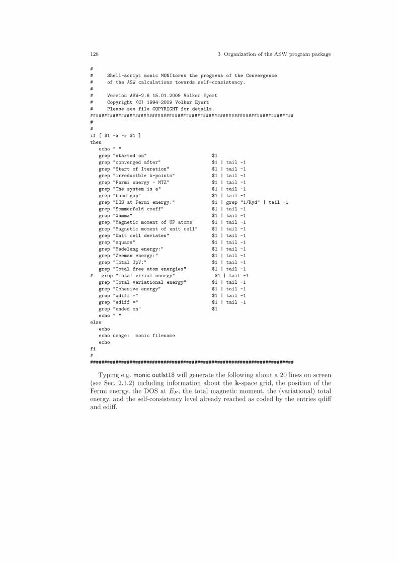
128 3 Organization of the ASW program package
#
# Shell-script monic MONItores the progress of the Convergence
# of the ASW calculations towards self-consistency.
#
# Version ASW-2.6 15.01.2009 Volker Eyert
# Copyright (C) 1994-2009 Volker Eyert
# Please see file COPYRIGHT for details.
########################################################################
#
#
if [ $1 -a -r $1 ]
then
echo " "
grep "started on" $1
grep "converged after" $1 | tail -1
grep "Start of Iteration" $1 | tail -1
grep "irreducible k-points" $1 | tail -1
grep "Fermi energy - MTZ" $1 | tail -1
grep "The system is a" $1 | tail -1
grep "band gap" $1 | tail -1
grep "DOS at Fermi energy:" $1 | grep "1/Ryd" | tail -1
grep "Sommerfeld coeff" $1 | tail -1
grep "Gamma" $1 | tail -1
grep "Magnetic moment of UP atoms" $1 | tail -1
grep "Magnetic moment of unit cell" $1 | tail -1
grep "Unit cell deviates" $1 | tail -1
grep "square" $1 | tail -1
grep "Madelung energy:" $1 | tail -1
grep "Zeeman energy:" $1 | tail -1
grep "Total 3pV:" $1 | tail -1
grep "Total free atom energies" $1 | tail -1
# grep "Total virial energy" $1 | tail -1
grep "Total variational energy" $1 | tail -1
grep "Cohesive energy" $1 | tail -1
grep "qdiff =" $1 | tail -1
grep "ediff =" $1 | tail -1
grep "ended on" $1
echo " "
else
echo
echo usage: monic filename
echo
fi
#
########################################################################
Typing e.g. monic outlst18 will generate the following about a 20 lines on screen(see Sec. 2.1.2) including information about the k-space grid, the position of theFermi energy, the DOS at EF , the total magnetic moment, the (variational) totalenergy, and the self-consistency level already reached as coded by the entries qdiffand ediff.
3.2 Plot programs and shell scripts 129
3.1.15 o2log
This utility shell script has turned out very useful in contracting the output files gen-erated during the self-consistent field calculations executed by program mnscf.run.In particular, with this shell script, output generated by intermediate iterations isremoved from the output files and only the portion of the most recent iteration iskept. Invoking o2log all will apply this procedure to all files with names beginningwith outlst, outblk, or outphn.
3.2 Plot programs and shell scripts
The plot programs coming with the distribution are distinguished from the mainprograms in that they do are completely independent of the CTRL file but startfrom files created by one of the main programs.
As for the main program there exist both executables (with ending “.run”) andcorresponding shell scripts (with ending “.x”), which latter call the executables andinclude an automatic call of the respective plot program as Gnuplot, RasMol orXCrysDen. In addition, intermediate files are deleted at the end. Whenever thesefiles are needed e.g. for exchange with other plot porgams one should employ theexecutable rather than the shell script. Again, we will use the names program,executable and shell script synonymously in the following discussion.
As an extra service to the user all specifications of the plot as entered during thedialog are echoed to a file PLIx, where x=B, D, C, K, O, P, R, S, or T dependingon the plot program. After the name of this file has been changed it can be editedand used for new plots by typing e.g. mnbnd.run < PLIBnew or mnbnd.x PLIBnew.
Another feature common to all plot programs concerns the title of the plot. Oninvoking any of the plot programs one is asked for specifying the title. Entering a“/” here will make the program use the title given by the first line of the CTRLfile. In addition, if you type & arbitrary text the title will be constructed from thefirst line of the CTRL file complemented by the “arbitrary text”.
3.2.1 plstr.run, plstr.x
This program starts from file STRU, which holds atomic positions and radii of allatoms within the plot region specified by tokens ORIGIN= and RPLOTn= andprepares for later use of RasMol. During the dialog colours and sizes of the atomicspheres as well as the plot perspective can be specified. By default the muffin-tinradii are used for plotting. Nevertheless, the radii may still be scaled. Each class ofatoms is given a default colour which also may be changed while running plstr.run.The shell script plstr.x, after running plstr.run, automatically invokes RasMol. In case
130 3 Organization of the ASW program package
you want to print out the 3D plot please specify the command”write ps stru.ps“
from within RasMol in order to create a postscript file stru.ps of the image.
3.2.2 plbnd.run, plbnd.x
This program allows for plotting of the (weighted) band structure. It start fromfile BNDE containing the E(k) for all bands and, if token ORBWGT=T has beenspecified, from file BNDV, which holds the corresponding eigenvectors. These dataare prepared for later plotting with either Gnuplot or LATEX. In the latter case theshell script plbnd.lx has to be used in addition. During the dialog invoked by callingplbnd.x among other things the energy scale and reference as well as the energywindow must be specified. An example has been given in Sec. 2.1.3.
If output should be prepared for Gnuplot the program usually creates a filebnd.ps, which holds a postscript copy of the plot. A particular nice feature arisesfrom specifying writing to a LATEX file. This will produce a file bnd.tex. Next youhave to invoke the shell script plbnd.lx (see below), which will run LATEX on a filenamed plbnd.tex, into which bnd.tex is included via LATEX’s input command. As aresult, in case the band structure is not too complicated, hence, file bnd.tex is nottoo large, a final file bnd.ps is created. This LATEX option is particularly suited forplotting weighted band structures.
In the latter situation another important feature comes in. First, you are asked tospecify the orbitals to be included. Actually, the program plots for each k-point andband the projection of a particular orbital onto the full wave function. Furthermore,the program allows to specify the coordinate system, within which the orbitalsare selected. This is particularly useful, when the crystal field split d orbitals of atransition metal atom are to be considered as in the prvious examples of FeS2 orCrO2. for this reason the plot routine asks for a rotation matrix, which can be givenin the same form as the symmetry matrices in token SYMOPS of the CTRL file.See Chap. 4 for more details and examples. Alternatively, the string characterizingthe rotation can be written to a file named ROTS. In that case just enter “f” in thedialog.
3.2.3 pldos.run, pldos.x
The plot program pldos.x enables plotting of the total and partial densities of states(DOS). Both the DOS itself and the integrated DOS can be displayed. Input isread from file DOS. Intermediate files are prepared for both Gnuplot and LATEX.However, for the DOS, Gnuplot produces a nicer output, usually contained in thepostscript file dos.ps.
During the dialog the user is asked for the energy window, scale, and reference. Inaddition, for each curve the orbitals to be included and a scaling factor must be spec-

3.2 Plot programs and shell scripts 131
ified. Finally, the curve can be broadened by folding with a Gaussian, a Lorentzian,the Fermi function, or a combination of these. This is useful especially for a com-parison with experimental results. While for Gaussian broadening a constant widthcan be specified, the Lorentzian broadening allows for an energy dependent widthof the form wL = wL0 + wL1(E − EF )2. Such an energy dependent broadening isuseful for comparison to experiments where lifetime effects might play a role.
As for the band structure plots, a rotation matrix can be specified for each curvein order to make the program refer the orbitals to a rotated coordinate system.While in prior versions, the use of local coordinate systems in the plot routineswas restricted to rotations with angle equal to one digit integer divisions of the fullcircle, this restriction has been removed in the later versions. As a consequence,rotations may be specified as
”RiA“ as before, where A is the axis and i is a one
digit integer division of the full circle. In addition, the respective plot programsaccepts the notation
”R(ii)A“, where
”ii“ must be an integer specifying the angle
in degrees, i.e. it can be any integer between -360 and +360. The assumption ofinteger angles should be sufficient for most cases.
For magnetic systems, there is a choice for each curvei. The program can displaythe contribution from only one spin or from both spins as well as their sum anddifference, respectively. Finally, the total number of curves generated by the programis limited to nine.
3.2.4 plcop.run, plcop.x
This program must be used for plotting the total and partial crystal orbital overlappopulation (COOP). Again, also the integrated quantities can be plotted. Input isread from file COOP. If Gnuplot is specified for output usually a file coop.ps. Thedialog proceeds in much the same way as for pldos.x. However, note that for eachcurve two orbitals have to given.
3.2.5 plopt.run, plopt.x
This program allows to plot the optical properties as the optical conductivity, dielec-tric function, index of refraction, extinction coefficient, optical reflectivity, opticalabsorption, and the energy-loss function. In addition to the interband contributions,the calculated plasma frequency can be used to include the intraband terms.
Input is read from file OPT and output is generated for use with Gnuplot, whichby default writes to a postscript file opt.ps.

132 3 Organization of the ASW program package
3.2.6 pltrp.run, pltrp.x
This program allows to plot the transport and thermoelectric properties. Their eval-uation is performed within Boltzmann transport theory. Calculations include theelectrical conductivity and resistivity, the thermopower, the power factor, the elec-trothermal figure of merit, the thermal conductivity, as well as the Hall conductivityand coefficient. The calculation of these properties is initiated by setting the newtoken, SAVTRP=T and running mnscf.run. The calculations work with all Brillouinzone integration schemes. However, use of BZINT=HPS should be avoided due tothe strong oscillations near the band edges, which leads to wrong results especiallyfor the thermopower and related quantities of doped semiconductors. This is essen-tially due to the fact that the thermopower is based on an energy integration in anarrow range around the Fermi energy, which is then most affected by the oscislla-tions. Plotting is done with a new routine, pltrp.run, which behave much like theother plotting routines. Input is echoed to the file PLIT. The plotting routine alsoallows to take into account the effect of doping within a rigid band scheme.
Input is read from file TRAP and output is generated for use with Gnuplot,which by default writes to a postscript file trap.ps.
3.2.7 plfre.run, plfre.x
This program starts from file FREE, which holds the overlapping free atom chargedensities and potential within the plot region specified by tokens ORIGIN= andRPLOTn=. It prepares for later use of Gnuplot. During the dialog you can choosebetween a contour or 3D plot. In addition, plot of the core charge density, valencecharge density or both or else the potential can be specified.
3.2.8 plbnd.lx, pldos.lx, plcop.lx, plopt.lx, pltrp.lx
These shell script include files bnd.tex, dos.tex, coop.tex, opt.tex, and trap.tex intothe LATEX envelope files plbnd.tex, pldos.tex, plcop.tex, plopt.tex, and pltrp.tex,respectively, and run LATEX as well as dvips. As a result, postscript files bnd.ps,dos.ps, coop.ps, opt.ps, and trap.ps, respectively, are obtained.
3.2.9 plbnd.tex, pldos.tex, plcop.tex, plopt.tex, pltrp.tex
These are LATEX envelope files used to include bnd.tex, dos.tex, coop.tex, opt.tex,and trap.tex, respectively, and to produce postscript files of the band structure,DOS, COOP, optical and transport properties.
3.4 General purpose files 133
3.3 Installation shell scripts
3.3.1 Makefile
This is the makefile of the ASW program package for compiling and linking thesource and object files in a Unix/Linux environment. Typing make all will automat-ically create all executables and typing make install will install them in a prespecifieddirectory. A full description of this process has already been given in Sec. 1.4.
3.3.2 mkall.x
The compiling and linking step can be performed as a background job by invokingthe shell script mkall.x.
3.3.3 upshl
This shell script updates the specification of the directory, where the executablesare installed, in all shell scripts listed in Secs. 3.1 and 3.2. It is automatically calledduring the make install process.
3.4 General purpose files
Input data as well as data created by the ASW programs are spread over a largenumber of files. Yet, exchange of the user with the programs is limited essentially toa single file, i.e. the CTRL file. All other files serve the purpose of holding specificinformation about the distribution or are meant for information exchange betweendifferent programs. Neither of these latter files has to be changed by the user.Anyway, in the following list a short description is given for all files.
3.4.1 README
The README comprises a shortcut version of this user guide. Actually, the presentmanuscript has its roots in the README file. It contains very brief informationabout the distribution, installation and execution of the programs as well as someremarks about external software to be used with the ASW program package.
134 3 Organization of the ASW program package
3.4.2 INSTALL
A concise description of the installation process is provided by this file.
3.4.3 COPYRIGHT
The COPYRIGHT file covers all the copyright information concerning the ASWprogram package. It is printed in Sec. 1.6 and should be read by any user at thevery beginning.
3.4.4 LICENCE
The LICENCE file contains a single line indicating the expiration date for thepresent licence.
3.5 CTRL files
Input data as well as data created by the ASW programs are spread over a largenumber of files. Yet, exchange of the user with the programs is limited essentially toa single file, i.e. the CTRL file. All other files serve the purpose of holding specificinformation about the distribution or are meant for information exchange betweendifferent programs. Neither of these latter files has to be changed by the user.Anyway, in the following list a short description is given for all files.
3.5.1 CTRL
The CTRL file is the one and only input file to the main programs. It
• is fully free format and thus allows for a flexible setup,• is subdivided in sections (categories) each containing• a set of catchwords (tokens),• has many options,• many useful defaults.
The CTRL file contains information about
• the crystal structure,• the constituent atoms,
3.6 Information files 135
• the symmetry lines,• settings for input/output,• parameters for sphere packing,• Brillouin zone sampling,• iteration acceleration,• and convergence criteria.
All files following in the present list are automatically created and deleted by theprograms. A complete description of the CTRL file and all its categories and tokensis given in Chap. 4.
3.5.2 CBAK
All the main programs except for mnmpr.run write an updated copy of the CTRLfile to file CBAK unless a different name is specified by token WRITE= in categoryIO.
3.5.3 CALL
If the verbosity is set to 40 or a higher values this file is written by all the mainprograms except for mnmpr.run. As the file CBAK it holds an updated copy ofthe CTRL. However, in contrast to CBAK it contains all categories and tokensirrespective of their appearance in the CTRL file.
3.5.4 CNEW
The packing program mnpac.run writes a new CTRL file named CNEW (remember:file CTRL is never written to), which includes possibly created empty sphere posi-tions as well as the radii of all spheres. Before proceeding with the self-consistentcalculations you must rename the file CNEW to CTRL.
3.6 Information files
Input data as well as data created by the ASW programs are spread over a largenumber of files. Yet, exchange of the user with the programs is limited essentially toa single file, i.e. the CTRL file. All other files serve the purpose of holding specificinformation about the distribution or are meant for information exchange between
136 3 Organization of the ASW program package
different programs. Neither of these latter files has to be changed by the user.Anyway, in the following list a short description is given for all files.
3.6.1 HELP
A first overview over the capabilities of the ASW program package can be bestobtained by creating the HELP file. In case this is missing in the distribution it canbe most easily obtained by writing the line
IO HELP=T
to the CTRL and running any of the ASW main programs (those starting with“mn”). This will generate the HELP file listed here.
HELP-file for ASW-2.6
category HEADER
title
category VERSION
token ASW- of cast double
Version/release of program which has written CTRL
category IO
token HELP= of cast logical
Switch to print HELP file
token SHOW= of cast logical
Switch to echo CTRL file to output
token VERBOS= of cast integer
Verbosity level for printing of output
token CLEAN= of cast logical
Switch to shrink atomic files after convergence
token WRITE= of cast character
Name of file to which a copy of CTRL file is written
token EXTENS= of cast character
Default extension for all files besides CTRL file
category OPTIONS
token REL= of cast logical
Switch to scalar-relativistic mode
token LSCPL= of cast logical
Switch to turn on LS-coupling
token NSPIN= of cast integer
Number of spin-channels
token AFSYM= of cast logical
Switch to use antiferromagnetic symmetry if present
token BEXT= of cast double
External magnetic field (in z-direction)
token XCPAR= of cast character
String for XC-parametrization
3.6 Information files 137
token GGA= of cast character
String for GGA-parametrization
token LDA+U= of cast character
String for LDA+U-flavor
token OVLCHK= of cast logical
Switch to perform overlap check
token DISTL= of cast double
Maximum distance between atoms in the neighbour list
token CCOR= of cast logical
Switch to use combined correction to the ASA
token CORDRD= of cast logical
Switch to frozen-core calculations
category STRUC (mandatory)
token UNITS= of cast character
Units to be used in STRUC and SUPCELL
token ALAT= of cast double (mandatory)
Lattice constant A in UNITS
token PLAT= of cast double and length 9 (mandatory) --- OR:
Primitive translations in units of A
[
token SLAT= of cast character
String for Bravais lattice (obsolete)
token BLAT= of cast double --- OR:
Lattice constant B in UNITS
token BBYA= of cast double
Ratio of the lattice constants B/A
token CLAT= of cast double --- OR:
Lattice constant C in UNITS
token CBYA= of cast double
Ratio of the lattice constants C/A
token ALPHA= of cast double
Angle alpha
token BETA= of cast double
Angle beta
token GAMMA= of cast double
Angle gamma
]
token CNTR= of cast character
Centering type of the Bravais lattice
token ADJLAT= of cast logical
Switch to allow for adjusting the lattice
category CLASS (mandatory)
token NCLASS= of cast integer
Number of different atoms (classes)
token ATOM= of cast character (mandatory)
Class labels
token Z= of cast integer (mandatory)
Atomic numbers
token R= of cast double --- OR:
Atomic sphere radii in atomic units
token R/RA= of cast double
Atomic sphere radii in arbitrary units (obsolete)

138 3 Organization of the ASW program package
token LMXL= of cast integer
Maximum angular momentum including the lower waves
token LMXI= of cast integer
Maximum angular momentum including intermediate waves
token CONF= of cast integer and length 4
Principal quantum numbers for all orbitals
token COORB= of cast integer
Orbitals to be included in the COOP
token QVAL= of cast double and length 4
Valence charges for starting from scratch
token MVAL= of cast double and length 4
Valence moments for starting spinpolarized calculations
token UVAL= of cast double and length 4
Screened Coulomb parameters U for all orbitals
token JVAL= of cast double and length 4
Screened Stoner parameters J for all orbitals
category SITE (mandatory)
token NBAS= of cast integer
Number of atoms
token CARTP= of cast logical
Switch to treat atomic positions as Cartesian
token CHOUT= of cast logical
Switch to change interpretation of atomic positions
token ADJPOS= of cast logical
Switch to allow for adjusting the atomic positions
token ATOM= of cast character (mandatory)
Class labels
token POS= of cast double and length 3 (mandatory)
Positions of basis atoms
token SPIN= of cast character
String characterizing the spin direction
category SYMGRP
token GENPOS= of cast logical
Switch to complete atomic basis by use of symmetry
token CARTR= of cast logical
Switch to treat rotation axes as Cartesian
token CARTT= of cast logical
Switch to treat fractional translations as Cartesian
token ORIGIN= of cast integer
Origin choice
token SGSYM= of cast character --- OR:
Space group symbol
token SGNUM= of cast integer --- OR:
Space group number
token SYMOPS= of cast character and length 48
Strings for space group generators
category PACK
token FILLNG= of cast double
Filling factor for atomic sphere volumes
token OBYDMX= of cast double
Maximum allowed overlap/distance
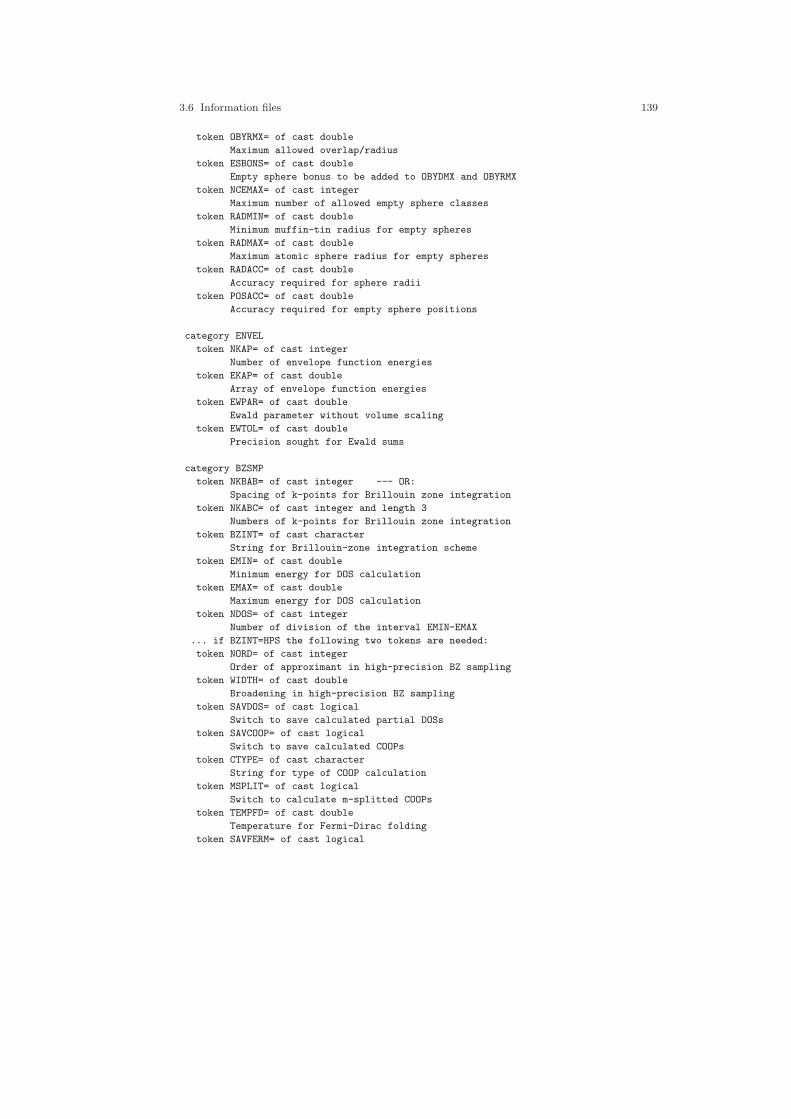
3.6 Information files 139
token OBYRMX= of cast double
Maximum allowed overlap/radius
token ESBONS= of cast double
Empty sphere bonus to be added to OBYDMX and OBYRMX
token NCEMAX= of cast integer
Maximum number of allowed empty sphere classes
token RADMIN= of cast double
Minimum muffin-tin radius for empty spheres
token RADMAX= of cast double
Maximum atomic sphere radius for empty spheres
token RADACC= of cast double
Accuracy required for sphere radii
token POSACC= of cast double
Accuracy required for empty sphere positions
category ENVEL
token NKAP= of cast integer
Number of envelope function energies
token EKAP= of cast double
Array of envelope function energies
token EWPAR= of cast double
Ewald parameter without volume scaling
token EWTOL= of cast double
Precision sought for Ewald sums
category BZSMP
token NKBAB= of cast integer --- OR:
Spacing of k-points for Brillouin zone integration
token NKABC= of cast integer and length 3
Numbers of k-points for Brillouin zone integration
token BZINT= of cast character
String for Brillouin-zone integration scheme
token EMIN= of cast double
Minimum energy for DOS calculation
token EMAX= of cast double
Maximum energy for DOS calculation
token NDOS= of cast integer
Number of division of the interval EMIN-EMAX
... if BZINT=HPS the following two tokens are needed:
token NORD= of cast integer
Order of approximant in high-precision BZ sampling
token WIDTH= of cast double
Broadening in high-precision BZ sampling
token SAVDOS= of cast logical
Switch to save calculated partial DOSs
token SAVCOOP= of cast logical
Switch to save calculated COOPs
token CTYPE= of cast character
String for type of COOP calculation
token MSPLIT= of cast logical
Switch to calculate m-splitted COOPs
token TEMPFD= of cast double
Temperature for Fermi-Dirac folding
token SAVFERM= of cast logical

140 3 Organization of the ASW program package
Switch to save Fermi surface data
token SAVOPT= of cast logical
Switch to save calculated partial optical spectra
category CHARGE
token NETA= of cast integer
Number of charge density envelope function energies
token EETA= of cast double and length 2
Array of charge density envelope function energies
token SAVRHO= of cast logical
Switch to save calculated charge density
token SAVELF= of cast logical
Switch to save calculated electron localisation funct.
token CHARWIN= of cast logical
Switch to narrow down the charge density energy window
token EMINC= of cast double
Minimum energy for charge density calculation
token EMAXC= of cast double
Maximum energy for charge density calculation
category CONTROL
token START= of cast character
String controlling program starting point
token QUIT= of cast character
String controlling program end point
token FREE= of cast logical
Switch to free atom calculations / free electron bands
token NITBND= of cast integer
Maximum number of band iterations
token CNVG= of cast double
Convergence tolerance for zero moments
token CNVGET= of cast double
Convergence tolerance for total energy
token NITATM= of cast integer
Maximum number of intraatomic iterations
token CNVGQA= of cast double
Convergence tolerance for atomic charges
category MIXING
token NMIXB= of cast integer
Number of previous iterations used in band mixing
token BETAB= of cast double
Mixing parameter for band mixing
token INCBB= of cast logical
Switch to increase band mixing parameter
token NMIXA= of cast integer
Number of previous iterations used in atom mixing
token BETAA= of cast double
Mixing parameter for atom mixing
category SUPCELL
token ALAT= of cast double
Supercell lattice constant A in UNITS
token PLAT= of cast double and length 9 --- OR:

3.6 Information files 141
Supercell primitive translations in units of A
[
token SLAT= of cast character
String for supercell Bravais lattice (obsolete)
token BLAT= of cast double --- OR:
Supercell lattice constant B in UNITS
token BBYA= of cast double
Ratio of the supercell lattice constants B/A
token CLAT= of cast double --- OR:
Supercell lattice constant C in UNITS
token CBYA= of cast double
Ratio of the supercell lattice constants C/A
token ALPHA= of cast double
Angle alpha
token BETA= of cast double
Angle beta
token GAMMA= of cast double
Angle gamma
]
token CNTR= of cast character
Centering type of the supercell Bravais lattice
token EQUIV= of cast logical
Switch to keep subcells equivalent
token CARTS= of cast logical
Switch to treat position shift vector as Cartesian
token PSHIFT= of cast double and length 3
Shift vector for the supercell atomic positions
token CARTQ= of cast logical
Switch to treat spin wave vector as Cartesian
token QSWAVE= of cast double and length 3
Spin wave vector of (collinear) antiferromagnets
category SYMLIN
token NPAN= of cast integer
Number of symmetry lines (panels)
token NPTS= of cast integer
Maximum total number of points
token ORBWGT= of cast logical
Switch to calculate orbital weights
token SPATH= of cast logical
Switch to use spherical pathways
token EKPV0= of cast double
Photoelectron kinetic energy plus inner potential
token CPNORM= of cast double and length 3
Cleavage plane normal vector
token CARTN= of cast logical
Switch to treat normal vector as Cartesian
token CARTE= of cast logical
Switch to treat endpoints as Cartesian
token LABEL= of cast character
Labels of endpoints
token ENDPT= of cast double and length 3
Endpoints of symmetry lines

142 3 Organization of the ASW program package
category PLOT
token CARTV= of cast logical
Switch to treat plot vectors as Cartesian
token ORIGIN= of cast double and length 3
Origin of plot space
token RPLOT1= of cast double and length 3
Plot vector specifying plot space
token RPLOT2= of cast double and length 3
Plot vector specifying plot space
token RPLOT3= of cast double and length 3
Plot vector specifying plot space
token NPDIV1= of cast integer
Number of divisions of plot space
token NPDIV2= of cast integer
Number of divisions of plot space
token NPDIV3= of cast integer
Number of divisions of plot space
In addition, an output file is generated, which includes a full CTRL file, whereall categories and tokens are given with their default values. This output looks like
ASW-2.6, program MNSCF started on asterix at Tue, 10 Feb 2009, 14:42:00.
Copyright (C) 1992-2009 Volker Eyert
Please see file COPYRIGHT for details
Write information to file HELP for HELP=T:
SHOW=T lists default values for optional input.
Echo CTRL file for SHOW=T:
HEADER Cu fcc
data by Landolt-Boernstein
VERSION ASW-2.6
IO HELP=T SHOW=T VERBOS=30 CLEAN=T WRITE=CBAK EXTENS=
OPTIONS REL=T LSCPL=F NSPIN=1 AFSYM=F BEXT=0.0 XCPAR= GGA= LDA+U=FLL OVLCHK=T
DISTL=3.0 CCOR=T CORDRD=F
STRUC UNITS=BOHR ALAT=6.83079 PLAT= 0.0 0.0 0.0
0.0 0.0 0.0
0.0 0.0 0.0
SLAT= BLAT=6.83079 BBYA=1.0 CLAT=6.83079 CBYA=1.0 ALPHA=90.0 BETA=90.0
GAMMA=90.0 CNTR=F ADJLAT=F
CLASS NCLASS=1
ATOM=CU Z=29 R=2.6694476 R/RA=1.0 LMXL=2 LMXI=3 CONF=4 4 3 4
COORB=0 1 2
QVAL= 1.0 0.0 10.0 0.0 MVAL= 0.0 0.0 0.0 0.0
UVAL= 0.0 0.0 0.0 0.0 JVAL= 0.0 0.0 0.0 0.0
SITE NBAS=1 CARTP=T CHOUT=F ADJPOS=T
ATOM=CU POS= 0.0 0.0 0.0 SPIN=UP
SYMGRP GENPOS=F CARTR=T CARTT=F ORIGIN=1 SGSYM=Ia-3d SGNUM=230 SYMOPS=
PACK FILLNG=1.0 OBYDMX=0.15 OBYRMX=0.4 ESBONS=0.05 NCEMAX=1024 RADMIN=0.5

3.6 Information files 143
RADMAX=5.0 RADACC=1.0D-02 POSACC=1.0D-12
ENVEL NKAP=1 EKAP=-0.015 EWPAR=2.54950976 EWTOL=1.0D-10
BZSMP NKBAB=6 NKABC=0 0 0 BZINT=LTM EMIN=-1.0 EMAX=1.5 NDOS=2500
NORD=5 WIDTH=0.02 SAVDOS=F SAVCOOP=F CTYPE=ECOV MSPLIT=F TEMPFD=300.0
SAVFERM=F SAVOPT=F SAVTRAP=F
CHARGE NETA=2 EETA=-3.0 -5.0 SAVRHO=F SAVELF=F CHARWIN=F EMINC=-100.0
EMAXC=100.0
CONTROL START= QUIT= FREE=F NITBND=99 CNVG=1.0D-08 CNVGET=1.0D-08
NITATM=50 CNVGQA=1.0D-10
MIXING NMIXB=5 BETAB=0.5 INCBB=T NMIXA=5 BETAA=0.5
SUPCELL ALAT=6.83079 PLAT= 0.0 0.0 0.0
0.0 0.0 0.0
0.0 0.0 0.0
SLAT= BLAT=6.83079 BBYA=1.0 CLAT=6.83079 CBYA=1.0 ALPHA=90.0 BETA=90.0
GAMMA=90.0 CNTR=P EQUIV=T CARTS=T PSHIFT= 0.0 0.0 0.0 CARTQ=T
QSWAVE= 0.0 0.0 0.0
SYMLIN NPAN=5 NPTS=400 ORBWGT=T SPATH=F EKPV0=0.0 CPNORM= 0.0 0.0 0.0
CARTN=T CARTE=F
LABEL=W ENDPT= 0.500 0.250 0.750
LABEL=L ENDPT= 0.500 0.500 0.500
LABEL=g ENDPT= 0.000 0.000 0.000
LABEL=X ENDPT= 0.500 0.000 0.500
LABEL=W ENDPT= 0.500 0.250 0.750
LABEL=K ENDPT= 0.375 0.375 0.750
PLOT CARTV=T
ORIGIN= 0.0 0.0 0.0
RPLOT1= 1.0 0.0 0.0
RPLOT2= 0.0 1.0 0.0
RPLOT3= 0.0 0.0 1.0
NPDIV1=50 NPDIV2=50 NPDIV3=0
task 3, I/O : cpu time: 0.02800 sec
Execution stopping for HELP=T.
ASW-2.6, program MNSCF ended on asterix at Tue, 10 Feb 2009, 14:42:00.
3.6.2 SPCGRP
This file is written along with the HELP file. The SPCGRP file contains a list ofall 230 space groups, which for each entry gives the Bravais lattice, the numbers ofthe point and space group, respectively, the space group symbol in the Hermann-Mauguin notation, and the generators of the space group. The SPCGRP file is listedbelow.
SPCGRP-file for ASW-2.6
Lat PG SG O SG-Symbol Generators
tri 1 1 P1 E

144 3 Organization of the ASW program package
tri 2 2 P-1 I
sm 3 3 P2 R2Y
sm 3 3 P121 R2Y
sm 3 4 P2_1 R2Y:T(0,1/2,0)
sm 3 4 P12_11 R2Y:T(0,1/2,0)
cm 3 5 C2 R2Y
cm 3 5 A2 R2Y
cm 3 5 I2 R2Y
cm 3 5 C121 R2Y
cm 3 5 A121 R2Y
cm 3 5 I121 R2Y
sm 4 6 Pm MY
sm 4 6 P1m1 MY
sm 4 7 Pc MY:T(0,0,1/2)
sm 4 7 Pa MY:T(1/2,0,0)
sm 4 7 Pn MY:T(1/2,0,1/2)
sm 4 7 P1c1 MY:T(0,0,1/2)
sm 4 7 P1a1 MY:T(1/2,0,0)
sm 4 7 P1n1 MY:T(1/2,0,1/2)
cm 4 8 Cm MY
cm 4 8 Am MY
cm 4 8 Im MY
cm 4 8 C1m1 MY
cm 4 8 A1m1 MY
cm 4 8 I1m1 MY
cm 4 9 Cc MY:T(0,0,1/2)
cm 4 9 Cn MY:T(1/2,0,1/2)
cm 4 9 Aa MY:T(1/2,0,0)
cm 4 9 An MY:T(1/2,1/2,0)
cm 4 9 Ia MY:T(1/2,0,0)
cm 4 9 Ic MY:T(0,0,1/2)
cm 4 9 C1c1 MY:T(0,0,1/2)
cm 4 9 C1n1 MY:T(1/2,0,1/2)
cm 4 9 A1a1 MY:T(1/2,0,0)
cm 4 9 A1n1 MY:T(1/2,1/2,0)
cm 4 9 I1a1 MY:T(1/2,0,0)
cm 4 9 I1c1 MY:T(0,0,1/2)
sm 5 10 P2/m I MY
sm 5 10 P12/m1 I MY
sm 5 11 P2_1/m I MY:T(0,1/2,0)
sm 5 11 P12_1/m1 I MY:T(0,1/2,0)
cm 5 12 C2/m I MY
cm 5 12 A2/m I MY
cm 5 12 I2/m I MY
cm 5 12 C12/m1 I MY
cm 5 12 A12/m1 I MY
cm 5 12 I12/m1 I MY
sm 5 13 P2/c I MY:T(0,0,1/2)
sm 5 13 P2/a I MY:T(1/2,0,0)
sm 5 13 P2/n I MY:T(1/2,0,1/2)
sm 5 13 P12/c1 I MY:T(0,0,1/2)
sm 5 13 P12/a1 I MY:T(1/2,0,0)
sm 5 13 P12/n1 I MY:T(1/2,0,1/2)
sm 5 14 P2_1/c I MY:T(0,1/2,1/2)

3.6 Information files 145
sm 5 14 P2_1/a I MY:T(1/2,1/2,0)
sm 5 14 P2_1/n I MY:T(1/2,1/2,1/2)
sm 5 14 P12_1/c1 I MY:T(0,1/2,1/2)
sm 5 14 P12_1/a1 I MY:T(1/2,1/2,0)
sm 5 14 P12_1/n1 I MY:T(1/2,1/2,1/2)
cm 5 15 C2/c I MY:T(0,0,1/2)
cm 5 15 C2/n I MY:T(1/2,0,1/2)
cm 5 15 A2/a I MY:T(1/2,0,0)
cm 5 15 A2/n I MY:T(1/2,1/2,0)
cm 5 15 I2/a I MY:T(1/2,0,0)
cm 5 15 I2/c I MY:T(0,0,1/2)
cm 5 15 C12/c1 I MY:T(0,0,1/2)
cm 5 15 C12/n1 I MY:T(1/2,0,1/2)
cm 5 15 A12/a1 I MY:T(1/2,0,0)
cm 5 15 A12/n1 I MY:T(1/2,1/2,0)
cm 5 15 I12/a1 I MY:T(1/2,0,0)
cm 5 15 I12/c1 I MY:T(0,0,1/2)
so 6 16 P222 R2X R2Y
so 6 17 P222_1 R2X R2Y:T(0,0,1/2)
so 6 17 P22_12 R2X R2Y:T(0,1/2,0)
so 6 17 P2_122 R2X:T(1/2,0,0) R2Y
so 6 18 P22_12_1 R2X R2Y:T(0,1/2,1/2)
so 6 18 P2_122_1 R2X:T(1/2,0,1/2) R2Y
so 6 18 P2_12_12 R2X:T(1/2,1/2,0) R2Y:T(1/2,1/2,0)
so 6 19 P2_12_12_1 R2X:T(1/2,1/2,0) R2Y:T(0,1/2,1/2)
sco 6 20 C222_1 R2X R2Y:T(0,0,1/2)
sco 6 20 A2_122 R2X:T(1/2,0,0) R2Y
sco 6 20 B22_12 R2X R2Y:T(0,1/2,0)
sco 6 21 C222 R2X R2Y
sco 6 21 A222 R2X R2Y
sco 6 21 B222 R2X R2Y
fco 6 22 F222 R2X R2Y
bco 6 23 I222 R2X R2Y
bco 6 24 I2_12_12_1 R2X:T(0,0,1/2) R2Y:T(1/2,0,0)
so 7 25 Pmm2 MX MY
so 7 25 Pm2m MX MZ
so 7 25 P2mm MY MZ
so 7 26 Pmc2_1 MX MY:T(0,0,1/2)
so 7 26 Pcm2_1 MX:T(0,0,1/2) MY
so 7 26 Pm2_1b MX MZ:T(0,1/2,0)
so 7 26 Pb2_1m MX:T(0,1/2,0) MZ
so 7 26 P2_1ma MY MZ:T(1/2,0,0)
so 7 26 P2_1am MY:T(1/2,0,0) MZ
so 7 27 Pcc2 MX:T(0,0,1/2) MY:T(0,0,1/2)
so 7 27 Pb2b MX:T(0,1/2,0) MZ:T(0,1/2,0)
so 7 27 P2aa MY:T(1/2,0,0) MZ:T(1/2,0,0)
so 7 28 Pma2 MX:T(1/2,0,0) MY:T(1/2,0,0)
so 7 28 Pbm2 MX:T(0,1/2,0) MY:T(0,1/2,0)
so 7 28 Pm2a MX:T(1/2,0,0) MZ:T(1/2,0,0)
so 7 28 Pc2m MX:T(0,0,1/2) MZ:T(0,0,1/2)
so 7 28 P2mb MY:T(0,1/2,0) MZ:T(0,1/2,0)
so 7 28 P2cm MY:T(0,0,1/2) MZ:T(0,0,1/2)
so 7 29 Pca2_1 MX:T(1/2,0,1/2) MY:T(1/2,0,0)
so 7 29 Pbc2_1 MX:T(0,1/2,0) MY:T(0,1/2,1/2)

146 3 Organization of the ASW program package
so 7 29 Pb2_1a MX:T(1/2,1/2,0) MZ:T(1/2,0,0)
so 7 29 Pc2_1b MX:T(0,0,1/2) MZ:T(0,1/2,1/2)
so 7 29 P2_1ab MY:T(1/2,1/2,0) MZ:T(0,1/2,0)
so 7 29 P2_1ca MY:T(0,0,1/2) MZ:T(1/2,0,1/2)
so 7 30 Pnc2 MX:T(0,1/2,1/2) MY:T(0,1/2,1/2)
so 7 30 Pcn2 MX:T(1/2,0,1/2) MY:T(1/2,0,1/2)
so 7 30 Pn2b MX:T(0,1/2,1/2) MZ:T(0,1/2,1/2)
so 7 30 Pb2n MX:T(1/2,1/2,0) MZ:T(1/2,1/2,0)
so 7 30 P2an MY:T(1/2,1/2,0) MZ:T(1/2,1/2,0)
so 7 30 P2na MY:T(1/2,0,1/2) MZ:T(1/2,0,1/2)
so 7 31 Pmn2_1 MX MY:T(1/2,0,1/2)
so 7 31 Pnm2_1 MX:T(0,1/2,1/2) MY
so 7 31 Pn2_1m MX:T(0,1/2,1/2) MZ
so 7 31 Pm2_1n MX MZ:T(1/2,1/2,0)
so 7 31 P2_1mn MY MZ:T(1/2,1/2,0)
so 7 31 P2_1nm MY:T(1/2,0,1/2) MZ
so 7 32 Pba2 MX:T(1/2,1/2,0) MY:T(1/2,1/2,0)
so 7 32 Pc2a MX:T(1/2,0,1/2) MZ:T(1/2,0,1/2)
so 7 32 P2cb MY:T(0,1/2,1/2) MZ:T(0,1/2,1/2)
so 7 33 Pna2_1 MX:T(1/2,1/2,1/2) MY:T(1/2,1/2,0)
so 7 33 Pbn2_1 MX:T(1/2,1/2,0) MY:T(1/2,1/2,1/2)
so 7 33 Pc2_1n MX:T(1/2,0,1/2) MZ:T(1/2,1/2,1/2)
so 7 33 Pn2_1a MX:T(1/2,1/2,1/2) MZ:T(1/2,0,1/2)
so 7 33 P2_1nb MY:T(1/2,1/2,1/2) MZ:T(0,1/2,1/2)
so 7 33 P2_1cn MY:T(0,1/2,1/2) MZ:T(1/2,1/2,1/2)
so 7 34 Pnn2 MX:T(1/2,1/2,1/2) MY:T(1/2,1/2,1/2)
so 7 34 Pn2n MX:T(1/2,1/2,1/2) MZ:T(1/2,1/2,1/2)
so 7 34 P2nn MY:T(1/2,1/2,1/2) MZ:T(1/2,1/2,1/2)
sco 7 35 Cmm2 MX MY
sco 7 35 Bm2m MX MZ
sco 7 35 A2mm MY MZ
sco 7 36 Cmc2_1 MX MY:T(0,0,1/2)
sco 7 36 Ccm2_1 MX:T(0,0,1/2) MY
sco 7 36 Bb2_1m MX:T(0,1/2,0) MZ
sco 7 36 Bm2_1b MX MZ:T(0,1/2,0)
sco 7 36 A2_1ma MY MZ:T(1/2,0,0)
sco 7 36 A2_1am MY:T(1/2,0,0) MZ
sco 7 37 Ccc2 MX:T(0,0,1/2) MY:T(0,0,1/2)
sco 7 37 Bb2b MX:T(0,1/2,0) MZ:T(0,1/2,0)
sco 7 37 A2aa MY:T(1/2,0,0) MZ:T(1/2,0,0)
sco 7 38 Amm2 MX MY
sco 7 38 Bmm2 MX MY
sco 7 38 Am2m MX MZ
sco 7 38 Cm2m MX MZ
sco 7 38 B2mm MY MZ
sco 7 38 C2mm MY MZ
sco 7 39 Abm2 MX:T(0,1/2,0) MY:T(0,1/2,0)
sco 7 39 Bma2 MX:T(1/2,0,0) MY:T(1/2,0,0)
sco 7 39 Cm2a MX:T(1/2,0,0) MZ:T(1/2,0,0)
sco 7 39 Ac2m MX:T(0,1/2,0) MZ:T(0,1/2,0)
sco 7 39 B2cm MY:T(1/2,0,0) MZ:T(1/2,0,0)
sco 7 39 C2mb MY:T(1/2,0,0) MZ:T(1/2,0,0)
sco 7 40 Ama2 MX:T(1/2,0,0) MY:T(1/2,0,0)
sco 7 40 Bbm2 MX:T(0,1/2,0) MY:T(0,1/2,0)
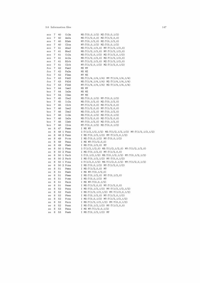
3.6 Information files 147
sco 7 40 Cc2m MX:T(0,0,1/2) MZ:T(0,0,1/2)
sco 7 40 Am2a MX:T(1/2,0,0) MZ:T(1/2,0,0)
sco 7 40 B2mb MY:T(0,1/2,0) MZ:T(0,1/2,0)
sco 7 40 C2cm MY:T(0,0,1/2) MZ:T(0,0,1/2)
sco 7 41 Aba2 MX:T(1/2,1/2,0) MY:T(1/2,1/2,0)
sco 7 41 Bba2 MX:T(1/2,1/2,0) MY:T(1/2,1/2,0)
sco 7 41 Cc2a MX:T(1/2,0,1/2) MZ:T(1/2,0,1/2)
sco 7 41 Ac2a MX:T(1/2,1/2,0) MZ:T(1/2,1/2,0)
sco 7 41 B2cb MY:T(1/2,1/2,0) MZ:T(1/2,1/2,0)
sco 7 41 C2cb MY:T(1/2,0,1/2) MZ:T(1/2,0,1/2)
fco 7 42 Fmm2 MX MY
fco 7 42 Fm2m MX MZ
fco 7 42 F2mm MY MZ
fco 7 43 Fdd2 MX:T(1/4,1/4,1/4) MY:T(1/4,1/4,1/4)
fco 7 43 Fd2d MX:T(1/4,1/4,1/4) MZ:T(1/4,1/4,1/4)
fco 7 43 F2dd MY:T(1/4,1/4,1/4) MZ:T(1/4,1/4,1/4)
bco 7 44 Imm2 MX MY
bco 7 44 Im2m MX MZ
bco 7 44 I2mm MY MZ
bco 7 45 Iba2 MX:T(0,0,1/2) MY:T(0,0,1/2)
bco 7 45 Ic2a MX:T(0,1/2,0) MZ:T(0,1/2,0)
bco 7 45 I2cb MY:T(1/2,0,0) MZ:T(1/2,0,0)
bco 7 46 Ima2 MX:T(1/2,0,0) MY:T(1/2,0,0)
bco 7 46 Ibm2 MX:T(0,1/2,0) MY:T(0,1/2,0)
bco 7 46 Ic2m MX:T(0,0,1/2) MZ:T(0,0,1/2)
bco 7 46 Im2a MX:T(1/2,0,0) MZ:T(1/2,0,0)
bco 7 46 I2mb MY:T(0,1/2,0) MZ:T(0,1/2,0)
bco 7 46 I2cm MY:T(0,0,1/2) MZ:T(0,0,1/2)
so 8 47 Pmmm I MX MY
so 8 48 1 Pnnn I:T(1/2,1/2,1/2) MX:T(1/2,1/2,1/2) MY:T(1/2,1/2,1/2)
so 8 48 2 Pnnn I MX:T(0,1/2,1/2) MY:T(1/2,0,1/2)
so 8 49 Pccm I MX:T(0,0,1/2) MY:T(0,0,1/2)
so 8 49 Pmaa I MX MY:T(1/2,0,0)
so 8 49 Pbmb I MX:T(0,1/2,0) MY
so 8 50 1 Pban I:T(1/2,1/2,0) MX:T(1/2,1/2,0) MY:T(1/2,1/2,0)
so 8 50 2 Pban I MX:T(0,1/2,0) MY:T(1/2,0,0)
so 8 50 1 Pncb I:T(0,1/2,1/2) MX:T(0,1/2,1/2) MY:T(0,1/2,1/2)
so 8 50 2 Pncb I MX:T(0,1/2,1/2) MY:T(0,0,1/2)
so 8 50 1 Pcna I:T(1/2,0,1/2) MX:T(1/2,0,1/2) MY:T(1/2,0,1/2)
so 8 50 2 Pcna I MX:T(0,0,1/2) MY:T(1/2,0,1/2)
so 8 51 Pmma I MX:T(1/2,0,0) MY
so 8 51 Pmmb I MX MY:T(0,1/2,0)
so 8 51 Pbmm I MX:T(0,1/2,0) MY:T(0,1/2,0)
so 8 51 Pcmm I MX:T(0,0,1/2) MY
so 8 51 Pmcm I MX MY:T(0,0,1/2)
so 8 51 Pmam I MX:T(1/2,0,0) MY:T(1/2,0,0)
so 8 52 Pnna I MX:T(0,1/2,1/2) MY:T(1/2,1/2,1/2)
so 8 52 Pnnb I MX:T(1/2,1/2,1/2) MY:T(1/2,0,1/2)
so 8 52 Pbnn I MX:T(0,1/2,0) MY:T(1/2,0,1/2)
so 8 52 Pcnn I MX:T(0,0,1/2) MY:T(1/2,1/2,1/2)
so 8 52 Pncn I MX:T(1/2,1/2,1/2) MY:T(0,0,1/2)
so 8 52 Pnan I MX:T(0,1/2,1/2) MY:T(1/2,0,0)
so 8 53 Pmna I MX MY:T(1/2,0,1/2)
so 8 53 Pnmb I MX:T(0,1/2,1/2) MY

148 3 Organization of the ASW program package
so 8 53 Pbmn I MX:T(1/2,1/2,0) MY
so 8 53 Pcnm I MX:T(1/2,0,1/2) MY:T(1/2,0,1/2)
so 8 53 Pncm I MX:T(0,1/2,1/2) MY:T(0,1/2,1/2)
so 8 53 Pman I MX MY:T(1/2,1/2,0)
so 8 54 Pcca I MX:T(1/2,0,1/2) MY:T(0,0,1/2)
so 8 54 Pccb I MX:T(0,0,1/2) MY:T(0,1/2,1/2)
so 8 54 Pbaa I MX:T(0,1/2,0) MY:T(1/2,1/2,0)
so 8 54 Pcaa I MX:T(0,0,1/2) MY:T(1/2,0,0)
so 8 54 Pbcb I MX:T(0,1/2,0) MY:T(0,0,1/2)
so 8 54 Pbab I MX:T(1/2,1/2,0) MY:T(1/2,0,0)
so 8 55 Pbam I MX:T(1/2,1/2,0) MY:T(1/2,1/2,0)
so 8 55 Pmcb I MX MY:T(0,1/2,1/2)
so 8 55 Pcma I MX:T(1/2,0,1/2) MY
so 8 56 Pccn I MX:T(1/2,0,1/2) MY:T(0,1/2,1/2)
so 8 56 Pnaa I MX:T(0,1/2,1/2) MY:T(1/2,1/2,0)
so 8 56 Pbnb I MX:T(1/2,1/2,0) MY:T(1/2,0,1/2)
so 8 57 Pbcm I MX:T(0,1/2,0) MY:T(0,1/2,1/2)
so 8 57 Pcam I MX:T(1/2,0,1/2) MY:T(1/2,0,0)
so 8 57 Pmca I MX:T(1/2,0,0) MY:T(0,0,1/2)
so 8 57 Pmab I MX:T(1/2,0,0) MY:T(1/2,1/2,0)
so 8 57 Pbma I MX:T(1/2,1/2,0) MY:T(0,1/2,0)
so 8 57 Pcmb I MX:T(0,0,1/2) MY:T(0,1/2,0)
so 8 58 Pnnm I MX:T(1/2,1/2,1/2) MY:T(1/2,1/2,1/2)
so 8 58 Pmnn I MX MY:T(1/2,1/2,1/2)
so 8 58 Pnmn I MX:T(1/2,1/2,1/2) MY
so 8 59 1 Pmmn I:T(1/2,1/2,0) MX MY
so 8 59 2 Pmmn I MX:T(1/2,0,0) MY:T(0,1/2,0)
so 8 59 1 Pmnm I:T(1/2,0,1/2) MX MY:T(1/2,0,1/2)
so 8 59 2 Pmnm I MX:T(1/2,0,0) MY:T(1/2,0,1/2)
so 8 59 1 Pnmm I:T(0,1/2,1/2) MX:T(0,1/2,1/2) MY
so 8 59 2 Pnmm I MX:T(0,1/2,1/2) MY:T(0,1/2,0)
so 8 60 Pbcn I MX:T(1/2,1/2,0) MY:T(0,0,1/2)
so 8 60 Pcan I MX:T(0,0,1/2) MY:T(1/2,1/2,0)
so 8 60 Pnca I MX:T(1/2,1/2,1/2) MY:T(0,1/2,1/2)
so 8 60 Pnab I MX:T(1/2,1/2,1/2) MY:T(1/2,0,0)
so 8 60 Pbna I MX:T(0,1/2,0) MY:T(1/2,1/2,1/2)
so 8 60 Pcnb I MX:T(1/2,0,1/2) MY:T(1/2,1/2,1/2)
so 8 61 Pbca I MX:T(1/2,1/2,0) MY:T(0,1/2,1/2)
so 8 61 Pcab I MX:T(1/2,0,1/2) MY:T(1/2,1/2,0)
so 8 62 Pnma I MX:T(1/2,1/2,1/2) MY:T(0,1/2,0)
so 8 62 Pmnb I MX:T(1/2,0,0) MY:T(1/2,1/2,1/2)
so 8 62 Pbnm I MX:T(1/2,1/2,0) MY:T(1/2,1/2,1/2)
so 8 62 Pcmn I MX:T(1/2,0,1/2) MY:T(0,1/2,0)
so 8 62 Pmcn I MX:T(1/2,0,0) MY:T(0,1/2,1/2)
so 8 62 Pnam I MX:T(1/2,1/2,1/2) MY:T(1/2,1/2,0)
sco 8 63 Cmcm I MX MY:T(0,0,1/2)
sco 8 63 Ccmm I MX:T(0,0,1/2) MY
sco 8 63 Amma I MX:T(1/2,0,0) MY
sco 8 63 Amam I MX:T(1/2,0,0) MY:T(1/2,0,0)
sco 8 63 Bbmm I MX:T(0,1/2,0) MY:T(0,1/2,0)
sco 8 63 Bmmb I MX MY:T(0,1/2,0)
sco 8 64 Cmca I MX MY:T(1/2,0,1/2)
sco 8 64 Ccmb I MX:T(1/2,0,1/2) MY
sco 8 64 Abma I MX:T(1/2,1/2,0) MY

3.6 Information files 149
sco 8 64 Acam I MX:T(1/2,1/2,0) MY:T(1/2,1/2,0)
sco 8 64 Bbcm I MX:T(1/2,1/2,0) MY:T(1/2,1/2,0)
sco 8 64 Bmab I MX MY:T(1/2,1/2,0)
sco 8 65 Cmmm I MX MY
sco 8 65 Ammm I MX MY
sco 8 65 Bmmm I MX MY
sco 8 66 Cccm I MX:T(0,0,1/2) MY:T(0,0,1/2)
sco 8 66 Amaa I MX MY:T(1/2,0,0)
sco 8 66 Bbmb I MX:T(0,1/2,0) MY
sco 8 67 Cmma I MX MY:T(1/2,0,0)
sco 8 67 Cmmb I MX:T(1/2,0,0) MY
sco 8 67 Abmm I MX:T(0,1/2,0) MY
sco 8 67 Acmm I MX:T(0,1/2,0) MY:T(0,1/2,0)
sco 8 67 Bmcm I MX:T(1/2,0,0) MY:T(1/2,0,0)
sco 8 67 Bmam I MX MY:T(1/2,0,0)
sco 8 68 1 Ccca I:T(1/2,0,1/2) MX:T(1/2,0,1/2) MY:T(1/2,0,1/2)
sco 8 68 2 Ccca I MX:T(1/2,0,1/2) MY:T(0,0,1/2)
sco 8 68 1 Cccb I:T(1/2,0,1/2) MX:T(1/2,0,1/2) MY:T(1/2,0,1/2)
sco 8 68 2 Cccb I MX:T(0,0,1/2) MY:T(1/2,0,1/2)
sco 8 68 1 Abaa I:T(1/2,1/2,0) MX:T(1/2,1/2,0) MY:T(1/2,1/2,0)
sco 8 68 2 Abaa I MX:T(0,1/2,0) MY:T(1/2,1/2,0)
sco 8 68 1 Acaa I:T(1/2,1/2,0) MX:T(1/2,1/2,0) MY:T(1/2,1/2,0)
sco 8 68 2 Acaa I MX:T(0,1/2,0) MY:T(1/2,0,0)
sco 8 68 1 Bbcb I:T(1/2,1/2,0) MX:T(1/2,1/2,0) MY:T(1/2,1/2,0)
sco 8 68 2 Bbcb I MX:T(0,1/2,0) MY:T(1/2,0,0)
sco 8 68 1 Bbab I:T(1/2,1/2,0) MX:T(1/2,1/2,0) MY:T(1/2,1/2,0)
sco 8 68 2 Bbab I MX:T(1/2,1/2,0) MY:T(1/2,0,0)
fco 8 69 Fmmm I MX MY
fco 8 70 1 Fddd I:T(1/4,1/4,1/4) MX:T(1/4,1/4,1/4) MY:T(1/4,1/4,1/4)
fco 8 70 2 Fddd I MX:T(0,1/4,1/4) MY:T(1/4,0,1/4)
bco 8 71 Immm I MX MY
bco 8 72 Ibam I MX:T(0,0,1/2) MY:T(0,0,1/2)
bco 8 72 Imcb I MX MY:T(1/2,0,0)
bco 8 72 Icma I MX:T(0,1/2,0) MY
bco 8 73 Ibca I MX:T(0,0,1/2) MY:T(1/2,0,0)
bco 8 73 Icab I MX:T(0,1/2,0) MY:T(0,0,1/2)
bco 8 74 Imma I MX MY:T(0,1/2,0)
bco 8 74 Immb I MX:T(1/2,0,0) MY
bco 8 74 Ibmm I MX:T(0,0,1/2) MY
bco 8 74 Icmm I MX:T(0,1/2,0) MY:T(0,1/2,0)
bco 8 74 Imcm I MX:T(1/2,0,0) MY:T(1/2,0,0)
bco 8 74 Imam I MX MY:T(0,0,1/2)
st 9 75 P4 R4Z
st 9 76 P4_1 R4Z:T(0,0,1/4)
st 9 77 P4_2 R4Z:T(0,0,1/2)
st 9 78 P4_3 R4Z:T(0,0,-1/4)
ct 9 79 I4 R4Z
ct 9 80 I4_1 R4Z:T(1/2,0,-1/4)
st 10 81 P-4 S4Z
ct 10 82 I-4 S4Z
st 11 83 P4/m I R4Z
st 11 84 P4_2/m I R4Z:T(0,0,1/2)
st 11 85 1 P4/n I:T(1/2,1/2,0) R4Z:T(1/2,1/2,0)
st 11 85 2 P4/n I R4Z:T(1/2,0,0)
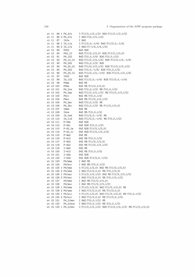
150 3 Organization of the ASW program package
st 11 86 1 P4_2/n I:T(1/2,1/2,1/2) R4Z:T(1/2,1/2,1/2)
st 11 86 2 P4_2/n I R4Z:T(0,1/2,1/2)
ct 11 87 I4/m I R4Z
ct 11 88 1 I4_1/a I:T(1/2,0,-1/4) R4Z:T(1/2,0,-1/4)
ct 11 88 2 I4_1/a I R4Z:T(-1/4,1/4,1/4)
st 12 89 P422 R4Z R2X
st 12 90 P42_12 R4Z:T(1/2,1/2,0) R2X:T(1/2,1/2,0)
st 12 91 P4_122 R4Z:T(0,0,1/4) R2X:T(0,0,1/2)
st 12 92 P4_12_12 R4Z:T(1/2,1/2,1/4) R2X:T(1/2,1/2,-1/4)
st 12 93 P4_222 R4Z:T(0,0,1/2) R2X
st 12 94 P4_22_12 R4Z:T(1/2,1/2,1/2) R2X:T(1/2,1/2,1/2)
st 12 95 P4_322 R4Z:T(0,0,-1/4) R2X:T(0,0,1/2)
st 12 96 P4_32_12 R4Z:T(1/2,1/2,-1/4) R2X:T(1/2,1/2,1/4)
ct 12 97 I422 R4Z R2X
ct 12 98 I4_122 R4Z:T(1/2,0,-1/4) R2X:T(1/2,0,-1/4)
st 13 99 P4mm R4Z MX
st 13 100 P4bm R4Z MX:T(1/2,1/2,0)
st 13 101 P4_2cm R4Z:T(0,0,1/2) MX:T(0,0,1/2)
st 13 102 P4_2nm R4Z:T(1/2,1/2,1/2) MX:T(1/2,1/2,1/2)
st 13 103 P4cc R4Z MX:T(0,0,1/2)
st 13 104 P4nc R4Z MX:T(1/2,1/2,1/2)
st 13 105 P4_2mc R4Z:T(0,0,1/2) MX
st 13 106 P4_2bc R4Z:T(0,0,1/2) MX:T(1/2,1/2,0)
ct 13 107 I4mm R4Z MX
ct 13 108 I4cm R4Z MX:T(0,0,1/2)
ct 13 109 I4_1md R4Z:T(1/2,0,-1/4) MX
ct 13 110 I4_1cd R4Z:T(1/2,0,-1/4) MX:T(0,0,1/2)
st 14 111 P-42m S4Z R2X
st 14 112 P-42c S4Z R2X:T(0,0,1/2)
st 14 113 P-42_1m S4Z R2X:T(1/2,1/2,0)
st 14 114 P-42_1c S4Z R2X:T(1/2,1/2,1/2)
st 14 115 P-4m2 S4Z MX
st 14 116 P-4c2 S4Z MX:T(0,0,1/2)
st 14 117 P-4b2 S4Z MX:T(1/2,1/2,0)
st 14 118 P-4n2 S4Z MX:T(1/2,1/2,1/2)
ct 14 119 I-4m2 S4Z MX
ct 14 120 I-4c2 S4Z MX:T(0,0,1/2)
ct 14 121 I-42m S4Z R2X
ct 14 122 I-42d S4Z R2X:T(1/2,0,-1/4)
st 15 123 P4/mmm I R4Z MX
st 15 124 P4/mcc I R4Z MX:T(0,0,1/2)
st 15 125 1 P4/nbm I:T(1/2,1/2,0) R4Z MX:T(1/2,1/2,0)
st 15 125 2 P4/nbm I R4Z:T(1/2,0,0) MX:T(0,1/2,0)
st 15 126 1 P4/nnc I:T(1/2,1/2,1/2) R4Z MX:T(1/2,1/2,1/2)
st 15 126 2 P4/nnc I R4Z:T(1/2,0,0) MX:T(0,1/2,1/2)
st 15 127 P4/mbm I R4Z MX:T(1/2,1/2,0)
st 15 128 P4/mnc I R4Z MX:T(1/2,1/2,1/2)
st 15 129 1 P4/nmm I:T(1/2,1/2,0) R4Z:T(1/2,1/2,0) MX
st 15 129 2 P4/nmm I R4Z:T(1/2,0,0) MX:T(1/2,0,0)
st 15 130 1 P4/ncc I:T(1/2,1/2,0) R4Z:T(1/2,1/2,0) MX:T(0,0,1/2)
st 15 130 2 P4/ncc I R4Z:T(1/2,0,0) MX:T(1/2,0,1/2)
st 15 131 P4_2/mmc I R4Z:T(0,0,1/2) MX
st 15 132 P4_2/mcm I R4Z:T(0,0,1/2) MX:T(0,0,1/2)
st 15 133 1 P4_2/nbc I:T(1/2,1/2,1/2) R4Z:T(1/2,1/2,1/2) MX:T(1/2,1/2,0)

3.6 Information files 151
st 15 133 2 P4_2/nbc I R4Z:T(1/2,0,1/2) MX:T(0,1/2,0)
st 15 134 1 P4_2/nnm I:T(1/2,1/2,1/2) R4Z:T(1/2,1/2,1/2) MX:T(1/2,1/2,1/2)
st 15 134 2 P4_2/nnm I R4Z:T(1/2,0,1/2) MX:T(0,1/2,1/2)
st 15 135 P4_2/mbc I R4Z:T(0,0,1/2) MX:T(1/2,1/2,0)
st 15 136 P4_2/mnm I R4Z:T(1/2,1/2,1/2) MX:T(1/2,1/2,1/2)
st 15 137 1 P4_2/nmc I:T(1/2,1/2,1/2) R4Z:T(1/2,1/2,1/2) MX
st 15 137 2 P4_2/nmc I R4Z:T(1/2,0,1/2) MX:T(1/2,0,0)
st 15 138 1 P4_2/ncm I:T(1/2,1/2,1/2) R4Z:T(1/2,1/2,1/2) MX:T(0,0,1/2)
st 15 138 2 P4_2/ncm I R4Z:T(1/2,0,1/2) MX:T(1/2,0,1/2)
ct 15 139 I4/mmm I R4Z MX
ct 15 140 I4/mcm I R4Z MX:T(0,0,1/2)
ct 15 141 1 I4_1/amd I:T(1/2,0,-1/4) R4Z:T(1/2,0,-1/4) MX
ct 15 141 2 I4_1/amd I R4Z:T(1/4,-1/4,1/4) MX
ct 15 142 1 I4_1/acd I:T(1/2,0,-1/4) R4Z:T(1/2,0,-1/4) MX:T(0,0,1/2)
ct 15 142 2 I4_1/acd I R4Z:T(1/4,-1/4,1/4) MX:T(0,0,1/2)
hex 16 143 P3 R3Z
hex 16 143 P311 R3Z
hex 16 144 P3_1 R3Z:T(0,0,1/3)
hex 16 144 P3_111 R3Z:T(0,0,1/3)
hex 16 145 P3_2 R3Z:T(0,0,-1/3)
hex 16 145 P3_211 R3Z:T(0,0,-1/3)
rho 16 146 R3 R3Z
rho 16 146 P31 R3Z
hex 17 147 P-3 I R3Z
hex 17 147 P-311 I R3Z
rho 17 148 R-3 I R3Z
rho 17 148 P-31 I R3Z
hex 18 149 P312 R3Z R2X
hex 18 150 P321 R3Z R2Y
hex 18 151 P3_112 R3Z:T(0,0,1/3) R2X
hex 18 152 P3_121 R3Z:T(0,0,1/3) R2Y:T(0,0,1/3)
hex 18 153 P3_212 R3Z:T(0,0,-1/3) R2X
hex 18 154 P3_221 R3Z:T(0,0,-1/3) R2Y:T(0,0,-1/3)
rho 18 155 R32 R3Z R2Y
rho 18 155 P32 R3Z R2Y
hex 19 156 P3m1 R3Z MY
hex 19 157 P31m R3Z MX
hex 19 158 P3c1 R3Z MY:T(0,0,1/2)
hex 19 159 P31c R3Z MX:T(0,0,1/2)
rho 19 160 R3m R3Z MY
rho 19 160 P3m R3Z MY
rho 19 161 R3c R3Z MY:T(0,0,1/2)
rho 19 161 P3c R3Z MY:T(1/2,1/2,1/2)
hex 20 162 P-31m I R3Z MX
hex 20 163 P-31c I R3Z MX:T(0,0,1/2)
hex 20 164 P-3m1 I R3Z MY
hex 20 165 P-3c1 I R3Z MY:T(0,0,1/2)
rho 20 166 R-3m I R3Z MY
rho 20 166 P-3m I R3Z MY
rho 20 167 R-3c I R3Z MY:T(0,0,1/2)
rho 20 167 P-3c I R3Z MY:T(1/2,1/2,1/2)
hex 21 168 P6 R6Z
hex 21 169 P6_1 R6Z:T(0,0,1/6)
hex 21 170 P6_5 R6Z:T(0,0,-1/6)

152 3 Organization of the ASW program package
hex 21 171 P6_2 R6Z:T(0,0,1/3)
hex 21 172 P6_4 R6Z:T(0,0,-1/3)
hex 21 173 P6_3 R6Z:T(0,0,1/2)
hex 22 174 P-6 S6Z
hex 23 175 P6/m I R6Z
hex 23 176 P6_3/m I R6Z:T(0,0,1/2)
hex 24 177 P622 R6Z R2X
hex 24 178 P6_122 R6Z:T(0,0,1/6) R2X:T(0,0,1/6)
hex 24 179 P6_522 R6Z:T(0,0,-1/6) R2X:T(0,0,-1/6)
hex 24 180 P6_222 R6Z:T(0,0,1/3) R2X:T(0,0,1/3)
hex 24 181 P6_422 R6Z:T(0,0,-1/3) R2X:T(0,0,-1/3)
hex 24 182 P6_322 R6Z:T(0,0,1/2) R2X:T(0,0,1/2)
hex 25 183 P6mm R6Z MX
hex 25 184 P6cc R6Z MX:T(0,0,1/2)
hex 25 185 P6_3cm R6Z:T(0,0,1/2) MX
hex 25 186 P6_3mc R6Z:T(0,0,1/2) MX:T(0,0,1/2)
hex 26 187 P-6m2 S6Z MY
hex 26 188 P-6c2 S6Z:T(0,0,1/2) MY:T(0,0,1/2)
hex 26 189 P-62m S6Z MX
hex 26 190 P-62c S6Z:T(0,0,1/2) MX:T(0,0,1/2)
hex 27 191 P6/mmm I R6Z MX
hex 27 192 P6/mcc I R6Z MX:T(0,0,1/2)
hex 27 193 P6_3/mcm I R6Z:T(0,0,1/2) MX
hex 27 194 P6_3/mmc I R6Z:T(0,0,1/2) MX:T(0,0,1/2)
sc 28 195 P23 R3D R2X
fcc 28 196 F23 R3D R2X
bcc 28 197 I23 R3D R2X
sc 28 198 P2_13 R3D R2X:T(1/2,1/2,0)
bcc 28 199 I2_13 R3D R2X:T(0,0,1/2)
sc 29 200 Pm-3 I R3D MX
sc 29 201 1 Pn-3 I:T(1/2,1/2,1/2) R3D MX:T(1/2,1/2,1/2)
sc 29 201 2 Pn-3 I R3D MX:T(0,1/2,1/2)
fcc 29 202 Fm-3 I R3D MX
fcc 29 203 1 Fd-3 I:T(1/4,1/4,1/4) R3D MX:T(1/4,1/4,1/4)
fcc 29 203 2 Fd-3 I R3D MX:T(0,1/4,1/4)
bcc 29 204 Im-3 I R3D MX
sc 29 205 Pa-3 I R3D MX:T(1/2,1/2,0)
bcc 29 206 Ia-3 I R3D MX:T(0,0,1/2)
sc 30 207 P432 R4X R3D
sc 30 208 P4_232 R4X:T(1/2,1/2,1/2) R3D
fcc 30 209 F432 R4X R3D
fcc 30 210 F4_132 R4X:T(1/4,1/4,1/4) R3D
bcc 30 211 I432 R4X R3D
sc 30 212 P4_332 R4X:T(-1/4,-1/4,1/4) R3D
sc 30 213 P4_132 R4X:T(1/4,1/4,-1/4) R3D
bcc 30 214 I4_132 R4X:T(1/4,1/4,-1/4) R3D
sc 31 215 P-43m S4X R3D
fcc 31 216 F-43m S4X R3D
bcc 31 217 I-43m S4X R3D
sc 31 218 P-43n S4X:T(1/2,1/2,1/2) R3D
fcc 31 219 F-43c S4X:T(1/2,1/2,1/2) R3D
bcc 31 220 I-43d S4X:T(1/4,1/4,-1/4) R3D
sc 32 221 Pm-3m I R4X R3D
sc 32 222 1 Pn-3n I:T(1/2,1/2,1/2) R4X R3D
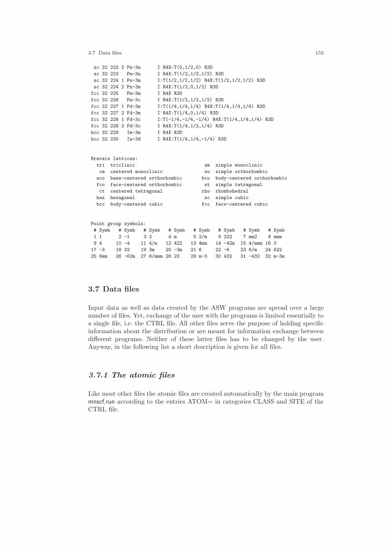
3.7 Data files 153
sc 32 222 2 Pn-3n I R4X:T(0,1/2,0) R3D
sc 32 223 Pm-3n I R4X:T(1/2,1/2,1/2) R3D
sc 32 224 1 Pn-3m I:T(1/2,1/2,1/2) R4X:T(1/2,1/2,1/2) R3D
sc 32 224 2 Pn-3m I R4X:T(1/2,0,1/2) R3D
fcc 32 225 Fm-3m I R4X R3D
fcc 32 226 Fm-3c I R4X:T(1/2,1/2,1/2) R3D
fcc 32 227 1 Fd-3m I:T(1/4,1/4,1/4) R4X:T(1/4,1/4,1/4) R3D
fcc 32 227 2 Fd-3m I R4X:T(1/4,0,1/4) R3D
fcc 32 228 1 Fd-3c I:T(-1/4,-1/4,-1/4) R4X:T(1/4,1/4,1/4) R3D
fcc 32 228 2 Fd-3c I R4X:T(1/4,1/2,1/4) R3D
bcc 32 229 Im-3m I R4X R3D
bcc 32 230 Ia-3d I R4X:T(1/4,1/4,-1/4) R3D
Bravais lattices:
tri triclinic sm simple monoclinic
cm centered monoclinic so simple orthorhombic
sco base-centered orthorhombic bco body-centered orthorhombic
fco face-centered orthorhombic st simple tetragonal
ct centered tetragonal rho rhombohedral
hex hexagonal sc simple cubic
bcc body-centered cubic fcc face-centered cubic
Point group symbols:
# Symb # Symb # Symb # Symb # Symb # Symb # Symb # Symb
1 1 2 -1 3 2 4 m 5 2/m 6 222 7 mm2 8 mmm
9 4 10 -4 11 4/m 12 422 13 4mm 14 -42m 15 4/mmm 16 3
17 -3 18 32 19 3m 20 -3m 21 6 22 -6 23 6/m 24 622
25 6mm 26 -62m 27 6/mmm 28 23 29 m-3 30 432 31 -432 32 m-3m
3.7 Data files
Input data as well as data created by the ASW programs are spread over a largenumber of files. Yet, exchange of the user with the programs is limited essentially toa single file, i.e. the CTRL file. All other files serve the purpose of holding specificinformation about the distribution or are meant for information exchange betweendifferent programs. Neither of these latter files has to be changed by the user.Anyway, in the following list a short description is given for all files.
3.7.1 The atomic files
Like most other files the atomic files are created automatically by the main programmnscf.run according to the entries ATOM= in categories CLASS and SITE of theCTRL file.

154 3 Organization of the ASW program package
Each atomic file contains all information about the atom at hand. Similar to theCTRL file it falls in eight categories named GEN, LDMT, ESJH, MOPT, VMTA,VLOC, RLOC, and CORE. They comprise the following data.
GEN Atomic number, angular momenta, valence state configuration, in-dicators for spin-polarized and relativistic calculations, informationabout the intraatomic radial mesh, core state orbitals, net atomiccharge, Madelung potential, muffin-tin zero, and total energy contri-butions.
LDMT Local density matrices as arising from the band calculation.
ESJH Hankel and Bessel energies and integrals for use in the intraatomicintegrals entering the secular matrix.
MOPT Intraatomic optical matrix elements.
VMTA Spherical symmetric intraatomic single-particle potential.
VLOC Intraatomic full potential.
RLOC Intraatomic full valence electron density.
CORE Core state energies and spherical symmetric intraatomic core electroncharge density.
An example atomic file looks like.
GEN: CU written by ASW-2.6
Z= 29 LMXL=2 LMXI=3 CONF= 4 4 3 4 NSPIN=1 REL=T
RMAX= 2.669448 NR= 541 AR= 0.20000000D-01 BR= 0.544565163250D-04
RMT= 2.367581 NRMT= 535
NCORE= 5 LCORE= 0 0 0 1 1 QCORE= 18
RHOV0= 0.1093061994D+03
NKAP=1 EKAP= -0.015000
VMTZ= -0.101593247946D+01
VRMAX= -0.101593247946D+01
EVBM= 0.114473077936D+01 ECBM= 0.515675388697D+00
EFMIN= 0.200000000000D+00 EFMAX= 0.120000000000D+01
EFERM= 0.681989411882D+00
ETFAT= -0.330455057198D+04 ETVAR= -0.330486846445D+04
LDMT: CU
WLLCC= 0.6864836706D+00 0.1523417630D-23 0.2757268709D-24 -0.2767936098D-25
0.1449338654D-18 -0.8122190416D-18 0.5788441776D-18 -0.1416149700D-18
0.1012977311D-17 0.0000000000D+00 0.0000000000D+00 0.0000000000D+00
...
...
...
WLLCA= 0.2702275600D-01 0.4885379417D-26 0.0000000000D+00 -0.1954151767D-25
0.4379444365D-18 -0.1298097441D-17 -0.5963111949D-18 -0.5638172905D-18

3.7 Data files 155
0.2394279798D-18 0.0000000000D+00 0.0000000000D+00 0.0000000000D+00
...
...
...
WLLAA= 0.2768160943D-01 -0.7908889916D-25 -0.2171968297D-25 0.1228003504D-25
0.7497342241D-19 -0.1895172744D-18 0.7678466682D-19 -0.1312662766D-18
0.1812971300D-18 0.3937420436D-26 -0.1003773840D-24 0.4368433128D-25
...
...
...
ESJH: CU
N L S EHAN EBES SHAN SBES
4 0 1 0.4443301305D+00 -0.6969317074D-01 0.6484687281D+00 0.5921039036D+01
4 1 1 0.1332828649D+01 -0.9136422052D-01 0.1704680720D+00 0.3102146828D+01
3 2 1 0.4790057314D+00 -0.3618341076D+00 0.3531087671D+01 0.8458719099D+00
4 3 1 0.4174489094D+01 -0.1191803276D+00 0.1012729572D+01 0.7191640791D-01
VHH= 0.9341213354D-02 -0.7375579101D-10 -0.7375579354D-10 -0.1391813866D-07
-0.3886705205D-08 -0.3886704598D-08 -0.3886709952D-08 -0.3886705255D-08
-0.3886702972D-08 -0.3461399420D-07 -0.3461399434D-07 -0.3461399448D-07
...
...
...
VHJ= 0.3310617248D-01 -0.2002889994D-09 -0.2002890054D-09 -0.4644303321D-07
-0.1026790881D-07 -0.1026790637D-07 -0.1026792824D-07 -0.1026790900D-07
-0.1026790013D-07 -0.9630564904D-07 -0.9630564952D-07 -0.9630565000D-07
...
...
...
VJJ= 0.1167285622D+00 -0.6451192721D-09 -0.6451192782D-09 -0.2364898375D-06
-0.6440567415D-08 -0.6440559472D-08 -0.6440628425D-08 -0.6440567963D-08
-0.6440541109D-08 -0.1431478215D-07 -0.1431478233D-07 -0.1431478252D-07
...
...
...
MOPT: CU
MHH= 0.0000000000D+00 -0.6507614309D-01 0.0000000000D+00 0.0000000000D+00
0.3235736296D+00 0.0000000000D+00 0.3937543036D+00 0.0000000000D+00
0.0000000000D+00 -0.2454696177D+00 0.0000000000D+00 -0.2979002690D+01
0.0000000000D+00 0.0000000000D+00 0.3301748000D+01 0.0000000000D+00
MHJ= 0.0000000000D+00 0.9557802382D-01 0.0000000000D+00 0.0000000000D+00
0.2135106097D+01 0.0000000000D+00 0.1862979714D+01 0.0000000000D+00
0.0000000000D+00 0.5727075033D+00 0.0000000000D+00 -0.5419268947D+00
0.0000000000D+00 0.0000000000D+00 0.6053496286D+00 0.0000000000D+00
MJH= 0.0000000000D+00 -0.4038246046D+00 0.0000000000D+00 0.0000000000D+00
0.8784526829D+00 0.0000000000D+00 -0.1146460821D+00 0.0000000000D+00
0.0000000000D+00 -0.8698565251D+00 0.0000000000D+00 -0.4041095516D+00
0.0000000000D+00 0.0000000000D+00 0.1538889316D+01 0.0000000000D+00
MJJ= 0.0000000000D+00 0.1451750170D+00 0.0000000000D+00 0.0000000000D+00
0.6378431349D+01 0.0000000000D+00 0.4516010729D+00 0.0000000000D+00
0.0000000000D+00 0.2616322297D+01 0.0000000000D+00 -0.6231920666D-01
0.0000000000D+00 0.0000000000D+00 0.6839972983D+00 0.0000000000D+00
VMTA: CU
NSPIN=1 RMAX= 2.669448 NR= 541 AR= 0.02000000 BR= 0.544565163250D-04
2.157039581415D+02 2.163036514691D+02 2.169282902168D+02 2.172948467082D+02

156 3 Organization of the ASW program package
2.175555310144D+02 2.177597897297D+02 2.179281747599D+02 2.180718055997D+02
2.181973599295D+02 2.183091431584D+02 2.184100915493D+02 2.185022968519D+02
...
...
...
2.540183818359D+01 2.492023067790D+01 2.444560720037D+01 2.397778672220D+01
2.351641175972D+01 2.306106447621D+01 2.261134947117D+01 2.216689282712D+01
2.172734163502D+01
A rather complex file check routine is invoked at the beginning of most of the mainprograms. During this check data from each atomic file is read in and compared tothe information gained from previous reading of the CTRL file. Whenever inconsis-tencies arise the program will issue a message and respond adequately. For instance,if the lattice constant is changed in the CTRL file, the program will identify theinconsistency of the sphere radii. In the following, the radii will be automaticallyadjusted and the program enforces an intraatomic restart calculation in order toupdate the intraatomic integrals for the secular matrix. In contrast, if the programdetects converged files but the CTRL files would require a start from scratch by thesetting START=REN the program stops in order not to overwrite the atomic files.Finally, if a spin-polarized calculation finds converged spin-degenerate files, startingvalues for the intraatomic magnetic moments are imposed and the program entersa restart calculation. Please see Sec. 2.3 and Chap. 4 for more detailed information.
3.7.2 FREE
The information about the overlapping free atom charge densities and potentialsas created by program mnfre.run go into this file. It is a formatted file, hence, it iswritten in ASCII.
3.7.3 STRU
This formatted file is written by all main programs. It contains the positions andcovalent radii of all atoms for later plotting with RasMol. All atoms within the plotregion specified in the CTRL file are included. However, in case this was not givenor not properly specified the unit cell is used instead.

3.7 Data files 157
3.7.4 STRX
This formatted file is written by all main programs. It contains the positions of allatoms. The file is written in XCrysDen’s xsf format and, hence, can be directly usedby XCrysDen. Just invoke
”xcrysden –xsf STRX“ or use the shell script plxcr.x.
3.7.5 BNDE
The formatted file BNDE contains the band structure E(k) as calculated as calcu-lated by program mnbnd.run.
3.7.6 BNDV
If required according to token ORBWGT=T the eigenvectors are written to theunformatted file BNDV by program mnbnd.run.
3.7.7 DOS
The unformatted file DOS is written by program mnscf.run if token SAVDOS=T isset. It contains the partial DOS for later plotting.
3.7.8 COOP
For SAVCOOP=T and the respective settings COORB= program mnscf.run createsan unformatted file COOP, which holds all information about the partial crystalorbital overlap populations (COOP), the crystal orbital Hamiltonian population(COHP) or the covalence energy (Ecov).
3.7.9 OPT
The unformatted file OPT is written by program mnscf.run if token SAVOPT=Tis set. It contains the different contributions to the optical conductivity for laterplotting.

158 3 Organization of the ASW program package
3.7.10 TRAP
The unformatted file TRAP is written by program mnscf.run if token SAVTRAP=Tis set. It contains the transport distribution and the related so-called Hall-distributionfor later plotting of the transport properties.
3.7.11 FERM
The formatted file FERM is written by program mnscf.run if the system is a metaland if token SAVFERM=T is set. It holds information about all bands straddlingthe Fermi energy, which are stored on a regular mesh. The file is in XCrysDen’s bxsfformat. Once the FERM file has been generated the Fermi surface can be plottedby the command
”xcrysden –bxsf FERM“ or use of the shell script plfrm.x.
3.7.12 RHO
This formatted file contains the electronic density (core and valence), their negativeLaplacians, and the effective potential. Depending on the dimensionality of the plotregion as specified in the CTRL file these data can be plotted using Gnuplot orXCrysDen.
3.7.13 Output files
Naming of the output files is completely free. However, if you are using the shellscripts mn***.x output is written to file out***, where the last three letters indicatethe type of the program. In contrast, shell script mnall.x writes output files outlstnn,where by default nn ranges from 6 to 18 according to the k-space grid.
3.8 Temporary files
Input data as well as data created by the ASW programs are spread over a largenumber of files. Yet, exchange of the user with the programs is limited essentially toa single file, i.e. the CTRL file. All other files serve the purpose of holding specificinformation about the distribution or are meant for information exchange betweendifferent programs. Neither of these latter files has to be changed by the user.Anyway, in the following list a short description is given for all files.
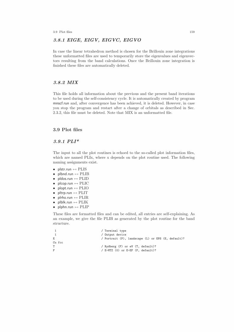
3.9 Plot files 159
3.8.1 EIGE, EIGV, EIGVC, EIGVO
In case the linear tetrahedron method is chosen for the Brillouin zone integrationsthese unformatted files are used to temporarily store the eigenvalues and eigenvec-tors resulting from the band calculations. Once the Brillouin zone integration isfinished these files are automatically deleted.
3.8.2 MIX
This file holds all information about the previous and the present band iterationsto be used during the self-consistency cycle. It is automatically created by programmnscf.run and, after convergence has been achieved, it is deleted. However, in caseyou stop the program and restart after a change of orbitals as described in Sec.2.3.2, this file must be deleted. Note that MIX is an unformatted file.
3.9 Plot files
3.9.1 PLI*
The input to all the plot routines is echoed to the so-called plot information files,which are named PLIx, where x depends on the plot routine used. The followingnaming assignments exist.
• plstr.run ↔ PLIS• plbnd.run ↔ PLIB• pldos.run ↔ PLID• plcop.run ↔ PLIC• plopt.run ↔ PLIO• pltrp.run ↔ PLIT• plrho.run ↔ PLIR• plblk.run ↔ PLIK• plphn.run ↔ PLIP
These files are formatted files and can be edited, all entries are self-explaining. Asan example, we give the file PLIB as generated by the plot routine for the bandstructure.
1 / Terminal type
1 / Output device
E / Portrait (P), landscape (L) or EPS (E, default)?
Cu fcc
T / Rydberg (F) or eV (T, default)?
F / E-MTZ (0) or E-EF (F, default)?
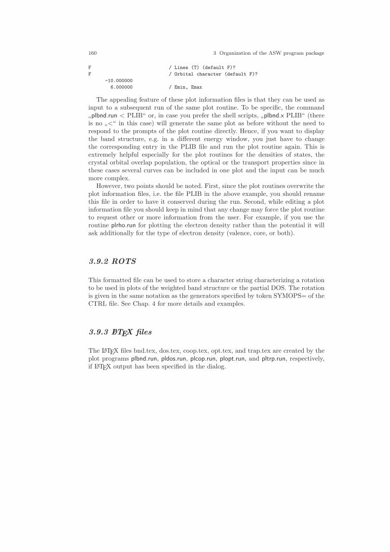
160 3 Organization of the ASW program package
F / Lines (T) (default F)?
F / Orbital character (default F)?
-10.000000
6.000000 / Emin, Emax
The appealing feature of these plot information files is that they can be used asinput to a subsequent run of the same plot routine. To be specific, the command
”plbnd.run < PLIB“ or, in case you prefer the shell scripts,
”plbnd.x PLIB“ (there
is no”<“ in this case) will generate the same plot as before without the need to
respond to the prompts of the plot routine directly. Hence, if you want to displaythe band structure, e.g. in a different energy window, you just have to changethe corresponding entry in the PLIB file and run the plot routine again. This isextremely helpful especially for the plot routines for the densities of states, thecrystal orbital overlap population, the optical or the transport properties since inthese cases several curves can be included in one plot and the input can be muchmore complex.
However, two points should be noted. First, since the plot routines overwrite theplot information files, i.e. the file PLIB in the above example, you should renamethis file in order to have it conserved during the run. Second, while editing a plotinformation file you should keep in mind that any change may force the plot routineto request other or more information from the user. For example, if you use theroutine plrho.run for plotting the electron density rather than the potential it willask additionally for the type of electron density (valence, core, or both).
3.9.2 ROTS
This formatted file can be used to store a character string characterizing a rotationto be used in plots of the weighted band structure or the partial DOS. The rotationis given in the same notation as the generators specified by token SYMOPS= of theCTRL file. See Chap. 4 for more details and examples.
3.9.3 LATEX files
The LATEX files bnd.tex, dos.tex, coop.tex, opt.tex, and trap.tex are created by theplot programs plbnd.run, pldos.run, plcop.run, plopt.run, and pltrp.run, respectively,if LATEX output has been specified in the dialog.

3.9 Plot files 161
3.9.4 Postscript files
The postscript files bnd.ps, dos.ps, coop.ps, opt.ps, trap.ps, and rho.ps are usuallycreated by the plot programs plbnd.run, pldos.run, plcop.run, plopt.run, pltrp.run, andplrho.run, respectively, if Gnuplot postscript output has been specified in the dialog.


Chapter 4
The main input file: CTRL
In this chapter we describe the structure and content of the CTRL file, which isthe main input file for the ASW package and, hence, the only interface between theuser and the main programs. Besides information on the crystal structure and theatoms making the crystal it contains also more technical parameters controlling theexecution. The CTRL file is fully free format, i.e. users do not have to obey anyformat specification. Yet, the file must not contain any tabulators (TABs).
It is important to notice that the CTRL file is exclusively used as an input file tothe programs. None of the programs writes to this file at all. Only some shell scripts,like “upctr”, are allowed to manipulate the CTRL file (see below). As a consequence,the CTRL file will never be destroyed even if you interrupt the program duringexecution or if your computer system crashes. Whenever the program creates newdata as e.g. empty sphere positions, atomic radii, or a supercell, it generates a newCTRL file called CNEW. In addition, most of the programs write an updated copyof CTRL to the file specified by the token WRITE=, which, by default, is CBAK.Finally, if the verbosity is increased, a file CALL is written, which comprises allpossible tokens and their default values, if not set otherwise in the CTRL file.
The CTRL file is grouped into categories each starting in the first column of thefile. Each category contains tokens specifying a portion of the input: e.g. in order tospecify the lattice constant you just write ALAT=6.76 somewhere in the categorySTRUC. A complete list of all categories and tokens is supplied in the file HELP,which is printed in Sec. 3.6. It is included as a separate file in the ASW package,but could be generated running any of the main programs with HELP=T specifiedin category IO of the CTRL file.
At present, the ASW program package interprets 142 tokens grouped in 17 dif-ferent categories. However, actually only entries in the three categories STRUC,CLASS, and SITE must be mandatorily specified by the user. For all other to-kens meaningful and well tested default values exist. For this reason, only very fewinformation is actually needed to successfully run the ASW program. Informationrequired from the user includes the crystal’s Bravais lattice, the type of atoms in thecrystal (their atomic numbers), and the positions of these species within the unit
163

164 4 The main input file: CTRL
cell of the crystal. The respective categories and tokens are indicated as mandatorybelow.
Once the program is started, it automatically creates the atomic files, which havethe names specified by token ATOM= in category CLASS. There is only one filefor each atom. In addition, the program creates a file for the mixing (file MIX);this file is deleted once self-consistency has been reached. Furthermore, in case thelinear tetrahedron method is chosen for the Brillouin zone integration, the programcreates and deletes the unformatted files EIGE, EIGV, EIGVC, and EIGVO, whichhold information about the eigenvalues and eigenvectors. Finally, the files DOS,COOP, OPT, TRAP (all unformatted), and FERM (formatted) are created andwritten to in case SAVDOS=T, SAVCOOP=T, SAVOPT=T, SAVTRAP=T andSAVFERM=T, respectively, are specified in category BZSMP.
A short version of the following explicit description is given in the HELP file,which comes with the distribution but can be easily created by specifying HELP=Tin category OPTIONS and running any of the ASW main programs. For this pur-pose, you may just construct a minimal CTRL file like
VERSION ASW-2.6IO HELP=T
and run any ASW program.
4.1 Category HEADER
This category is meant to hold a short description of the calculation. At present,this category is limited to 20 lines. Formally, the first line is treated differently fromthe following lines as it is interpreted as a title, which, by default, is appended tomost plots. For this reason, I recommend to specify only a short title in the first lineand to put longer comments into the following lines. Usually, I include referencesto important previous work on this compound in these lines.
4.2 Category VERSION
This category contains information about the version of the ASW package.
4.2.1 Token ASW- (cast real)
This token specifies the version and release number of the ASW program, whichhas been used to create the CTRL file or which you are intending to use, in caseyou have created the CTRL file by hand. The version and release number consists
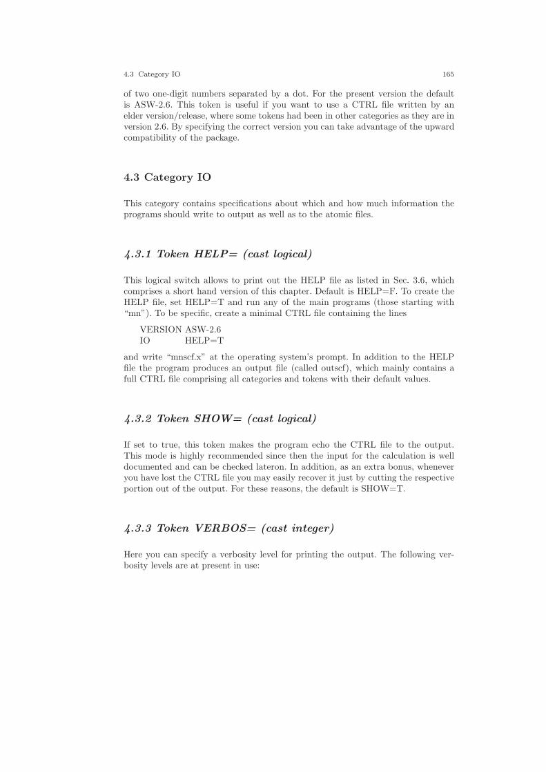
4.3 Category IO 165
of two one-digit numbers separated by a dot. For the present version the defaultis ASW-2.6. This token is useful if you want to use a CTRL file written by anelder version/release, where some tokens had been in other categories as they are inversion 2.6. By specifying the correct version you can take advantage of the upwardcompatibility of the package.
4.3 Category IO
This category contains specifications about which and how much information theprograms should write to output as well as to the atomic files.
4.3.1 Token HELP= (cast logical)
This logical switch allows to print out the HELP file as listed in Sec. 3.6, whichcomprises a short hand version of this chapter. Default is HELP=F. To create theHELP file, set HELP=T and run any of the main programs (those starting with“mn”). To be specific, create a minimal CTRL file containing the lines
VERSION ASW-2.6IO HELP=T
and write “mnscf.x” at the operating system’s prompt. In addition to the HELPfile the program produces an output file (called outscf), which mainly contains afull CTRL file comprising all categories and tokens with their default values.
4.3.2 Token SHOW= (cast logical)
If set to true, this token makes the program echo the CTRL file to the output.This mode is highly recommended since then the input for the calculation is welldocumented and can be checked lateron. In addition, as an extra bonus, wheneveryou have lost the CTRL file you may easily recover it just by cutting the respectiveportion out of the output. For these reasons, the default is SHOW=T.
4.3.3 Token VERBOS= (cast integer)
Here you can specify a verbosity level for printing the output. The following ver-bosity levels are at present in use:
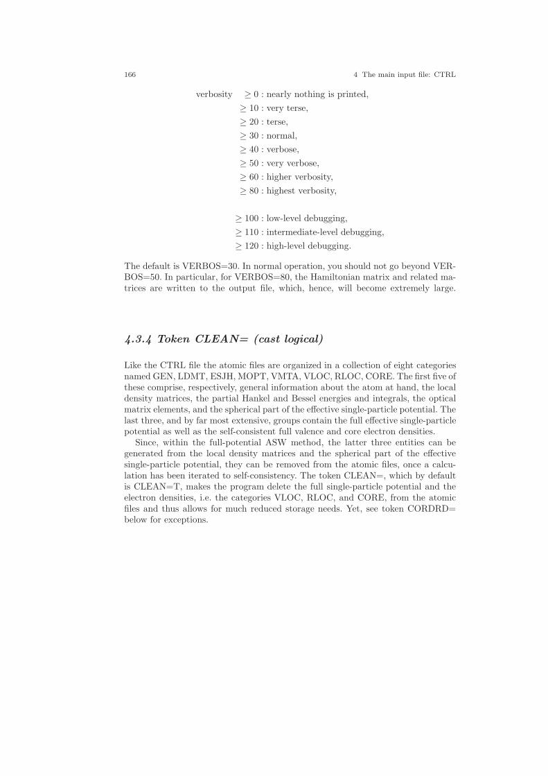
166 4 The main input file: CTRL
verbosity ≥ 0 : nearly nothing is printed,
≥ 10 : very terse,
≥ 20 : terse,
≥ 30 : normal,
≥ 40 : verbose,
≥ 50 : very verbose,
≥ 60 : higher verbosity,
≥ 80 : highest verbosity,
≥ 100 : low-level debugging,
≥ 110 : intermediate-level debugging,
≥ 120 : high-level debugging.
The default is VERBOS=30. In normal operation, you should not go beyond VER-BOS=50. In particular, for VERBOS=80, the Hamiltonian matrix and related ma-trices are written to the output file, which, hence, will become extremely large.
4.3.4 Token CLEAN= (cast logical)
Like the CTRL file the atomic files are organized in a collection of eight categoriesnamed GEN, LDMT, ESJH, MOPT, VMTA, VLOC, RLOC, CORE. The first five ofthese comprise, respectively, general information about the atom at hand, the localdensity matrices, the partial Hankel and Bessel energies and integrals, the opticalmatrix elements, and the spherical part of the effective single-particle potential. Thelast three, and by far most extensive, groups contain the full effective single-particlepotential as well as the self-consistent full valence and core electron densities.
Since, within the full-potential ASW method, the latter three entities can begenerated from the local density matrices and the spherical part of the effectivesingle-particle potential, they can be removed from the atomic files, once a calcu-lation has been iterated to self-consistency. The token CLEAN=, which by defaultis CLEAN=T, makes the program delete the full single-particle potential and theelectron densities, i.e. the categories VLOC, RLOC, and CORE, from the atomicfiles and thus allows for much reduced storage needs. Yet, see token CORDRD=below for exceptions.

4.4 Category OPTIONS 167
4.3.5 Token WRITE= (cast character)
Here you can specify the name of an updated backup version of the CTRL file,which will be written just before completion. The default is WRITE=CBAK.
4.3.6 Token EXTENS= (cast character)
Using this token you may specify a standard extension appended to all file namescreated by the program as e.g. “.dat” or “.DAT”. This is meant to conform withWINDOWS or VAX file name conventions. The default is empty, hence, all filenames come without an extension.
4.4 Category OPTIONS
The following tokens can be used to specify details of the calculations.
4.4.1 Token REL= (cast logical)
This token allows to switch between non-relativistic and scalar-relativistic mode.The default is REL=T (scalar-relativistic).
4.4.2 Token LSCPL= (cast logical)
In future versions this token will enable for including the LS-coupling, which, how-ever, is not yet implemented.
4.4.3 Token NSPIN= (cast integer)
Here you can specify the number of spin-channels. The default is NSPIN=1.

168 4 The main input file: CTRL
4.4.4 Token AFSYM= (cast logical)
In spin-polarized calculations, this token allows to use”spin-sublattice“ symmetry,
which preserves the electronic states on going from one sublattice to the otherand at the same time changing spins. This symmetry allows to perform the bandcalculation for one spin only and to extract the other spins results from the firstones. When AFSYM=T is specified, in addition, for each atom the
”direction“ of
spin has to be specified with the help of token SPIN= (see below). A more detaileddescription of how to perform spin-polarized calculations has been given in Secs.2.4 and 2.5.
4.4.5 Token BEXT= (cast double)
This token comprises an external magnetic field (in z-direction). The default valueis BEXT=0.0. Note that use of finite magnetic fields has not yet been fully tested.
4.4.6 Token XCPAR= (cast character)
Since version ASW-1.7, token XCPAR= enables specification of different LDAschemes. Actually, almost all known parametrizations are included now. The de-sired LDA parametrization is specified in the form XCPAR=P-S, where
P denotes the parametrization by
KSG: Kohn, Sham, and Gaspar (exchange only) [123,194]GLW: Gunnarsson, Lundqvist, and Wilkins [146]JMW: Janak, Moruzzi, and Williams [169]VBH: von Barth and Hedin [37]MJW: Moruzzi, Janak, and Williams [267]PZ: Perdew and Zunger [297]VWN: Vosko, Wilk, and Nusair [370]PW: Perdew and Wang [296]
andS denotes the spin interpolation by
GLW: Gunnarsson, Lundqvist, and Wilkins [146]VBH: von Barth and Hedin [37]VWN: Vosko, Wilk, and Nusair [370]PW: Perdew and Wang [296]

4.4 Category OPTIONS 169
Note that while the default was XCPAR=MJW-VBH in all versions up to ASW-1.6,it is now set to the more accurate XCPAR=VWN-VWN.
4.4.7 Token GGA= (cast character)
Since version ASW-1.8, a new token, GGA= has been included, which allows spec-ification of different schemes of the generalized gradient approximation (GGA).Possible GGA parametrizations are GGA=G where
G denotes the parametrization by
PW86 Perdew and Wang 1986 (GGA-I) [295]PW: Perdew and Wang 1991 (GGA-II) [227,289,293]EV: Engel and Vosko 1993 [100]PBE: Perdew, Burke, and Ernzerhof 1996 [290,292]ZY Zhang and Yang 1998 [401]WC Wu and Cohen 2006 [398]
The default is GGA= , which means to use none of these schemes.
4.4.8 Token LDA+U= (cast character)
Version 2.4 was the first version to allow for LDA+U calculations by specifying bythe token LDA+U= one of three schemes. They differ by the double-counting termsintroduced to avoid the double counting of electronic interactions within the LDAand the Hubbard model. Possible specifications are LDA+U=D where
D denotes the parametrization by
AMF: around mean field proposed byAnisimov, Zaanen, and Andersen 1991 [28]
FLL: fully localized limit proposed byAnisimov, Solovyev, Korotin, Czyzyk, and Sawatzky 1993 [27]
DFT: interpolation scheme proposed byPetukhov, Mazin, Chioncel, and Liechtenstein 2003 [299]
The default is LDA+U= , which means that the LDA+U scheme is not used.

170 4 The main input file: CTRL
4.4.9 Token OVLCHK= (cast logical)
In elder versions of the standard ASW method (and also the LMTO method) slightambiguities came in by bad settings of the atomic sphere radii. Most of such in-accuracies come from too large overlap of the spheres. In particular for the ASWmethod, the situation has much improved by the invention of the sphere geometryoptimization (SGO) algorthim, which allows to automatically evaluate the radii.However, it is still recommended to check the radii for too large overlap. This over-lap check is invoked by the token OVLCHK=, which, by default, is OVLCHK=T.In this case a list of atom pairs is generated, which, for each pair, holds the vectorbetween the respective atomic sites, their distance, the sum of the radii, the linearoverlap of the atomic spheres as well as the overlap scaled to the distance and theradii. Finally, each line may contain up to three exclamation marks indicating thatthe overlap scaled to the distance exceed 10%, 20%, and 30%, respectively.
4.4.10 Token DISTL= (cast double)
With this token a maximum distance between atoms can be specified (in atomicunits). Atom pairs with distance below this value will be included in the abovementioned list printed to the output. The default value is 3.0.
4.4.11 Token CCOR= (cast logical)
This switch enforces use of the socalled combined correction to the ASA. Actually,the term combined correction is more related to the LMTO method since most earlycalculations were done with the pure ASA. For this reason, calculations employingthe combined corrections earned an extra bonus. In contrast, in the ASW methodthese corrections to the ASA were included from the very beginning and, hence,calculations without the combined corrections actually were never done. Hence, thedefault is CCOR=T.
Since switching off the combined correction does not make sense in a full-potentialcode this token will most likely be removed in future versions.
4.4.12 Token CORDRD= (cast logical)
For some instances asi, e.g., calculation of rather small energy differences, it mightbe necessary to freeze the core state during the self-consistency cycle. This is allowedfor by setting CORDRD=T. Yet, the default is CORDRD=F.

4.5 Category STRUC (mandatory) 171
Note that in case of frozen core calculations the last of the above mentioned cat-egories contained in the atomic files, i.e. the category CORE must not be deletedfrom the file after successful convergence. As a consequence, for CORDRD=T speci-fying CLEAN=T will remove only the categories VLOC and RLOC from the atomicfiles, but will preserve the category CORE.
4.5 Category STRUC (mandatory)
This category holds all the information about the Bravais lattice. Of course, itspresence is necessary for any calculation.
4.5.1 Token UNITS= (cast character)
Here you can choose the units to be used for the following tokens, which may beatomic units (UNITS=BOHR, default) or Angstroems (UNITS=ANGS). Note thatthis choice also affects all input in category SUPCELL (see below).
4.5.2 Token ALAT= (mandatory; cast double)
This token contains the lattice constant in the units specified by token UNITS=.The default is ALAT=0.0. As a consequence, if the lattice constant is not given afinite value the program aborts.
Actually, the tokens ALAT= and PLAT= below are complementary in that eachof them can be scaled by a factor if the number(s) coming with the respectiveother token are scaled by the inverse. An equivalent statement holds for the tokensBBYA= and CBYA=, also given below. As a consequence, you may regard theinput given by ALAT= as a length scale for the whole crystal used for the primitivetranslations.
4.5.3 Token PLAT= (mandatory; cast double; length 9)
Information about the Bravais lattice is covered by this token, which contains thethree primitive translations ai, i = 1, 2, 3 in units of the lattice constant as specifiedby token ALAT=. All nine components must be given in the order a1x, a1y , a1z ,a2x, a2y, a2z , a3x, a3y, a3z .

172 4 The main input file: CTRL
4.5.4 Token SLAT= (cast character; marked obsolete)
As an alternative to explicitly specifying the primitive translations by PLAT= youmay use the following five tokens together with the token BETA=, which rely ondefault lattice vectors coded in the ASW package.
However, note that the token SLAT= is marked obsolete and the token CNTR=together with the tokens for the lattice constants and the angles should be usedinstead.
Token SLAT= indicates a string for the Bravais lattice. Possible values are
SC: simple cubicBCC: body-centered cubicFCC: face-centered cubicST: simple tetragonalBCT: body-centered tetragonalSO: simple orthorhombicSCO: base-centered orthorhombicBCO: body-centered orthorhombicFCO: face-centered orthorhombicSM: simple monoclinicSCM: base-centered monoclinicTRI: trigonalHEX: hexagonal
Note that the primitive translations coming with these specifications correspondto the definitions of Bradley and Cracknell, which in some instances deviate fromthe definitions commonly used. For this reason, you are strongly urged to check theprimitive translations, which are printed to output at the beginning of the programsexecution.
4.5.5 Token BLAT= (cast double)
For the other lattice constants coming with non-cubic and non-trigonal systemsthere exist two different ways of specification. Token BLAT= gives the lattice con-stant B explicitly in the units specified by token UNITS=. As for ALAT=, thedefault is BLAT=0.0.
4.5.6 Token BBYA= (cast double)
Alternatively, the lattice constant B can be specified by the token BBYA=, whichfixes the ratio of the lattice constants BLAT and ALAT. As for BLAT= above thedefault is BBYA=0.0.

4.5 Category STRUC (mandatory) 173
4.5.7 Token CLAT= (cast double)
Token CLAT= gives the lattice constant C explicitly in the units specified by tokenUNITS=. As for ALAT=, the default is CLAT=0.0.
4.5.8 Token CBYA= (cast double)
Alternatively, the token CBYA= allows to specify the lattice constant C in termsof the ratio of the lattice constants CLAT and ALAT. The default is CBYA=0.0.
4.5.9 Token ALPHA= (cast double)
With this token the angle between the second and third lattice vectors is specificed.The default value is ALPHA=90.0.
4.5.10 Token BETA= (cast double)
With this token the angle between the first and third lattice vectors is specificed.The default value is BETA=90.0.
4.5.11 Token GAMMA= (cast double)
With this token the angle between the first and second lattice vectors is specificed.The default value is GAMMA=90.0.
4.5.12 Token CNTR= (cast character)
With this token one of the following seven centering types of the Bravais lattice canbe selected.
P primitiveC face-centered on the a,b-planeB face-centered on the c,a-planeA face-centered on the b,c-planeI body-centered
174 4 The main input file: CTRL
F face-centeredR rhombohedral
The default value is CNTR=P.
4.5.13 Token ADJLAT= (cast logical)
If set to ADJLAT=T this switch allows the program to adjust the lattice vectorsto the optimal choice. The default is ADJLAT=F.
4.6 Category CLASS (mandatory)
Once the Bravais lattice has been specified the information about the crystal struc-ture is completed by giving the positions of the atoms within the unit cell as wellas the species of atoms, which hold these sites. While the present category com-prises all information about the atomic species, the atomic sites will be given in thefollowing section of the CTRL file.
4.6.1 Token NCLASS= (cast integer)
The number of different atoms, which we call classes of atoms, can be specified intwo different ways. The most comfortable and standard procdure consists of lettingthe programs count the number of ATOM= entries just below.
However, in the course of calculations it might be useful to exclude some of theclasses listed below from consideration by the program. This can be most easilyaccomplished by shifting the corresponding ATOM= entries to the end of this cat-egory and reducing the number of classes, which are taken into account by theprograms by setting NCLASS= to the reduced number of classes.
To summarize, if a number of classes is specified by a NCLASS=n entry theprogram tries to reads as many classes. Any subsequent ATOM= entries are ignored.On the other hand, if the are less ATOM= entries than specified by NCLASS=n,the program will warn for the missing classes and stop.
4.6.2 Token ATOM= (mandatory; cast character)
Here you must label each of the classes. In the course of the calculations these labelsare used to name the atomic files. My personal preference is to label classes by their

4.6 Category CLASS (mandatory) 175
names given in the periodic table extended by a roman number, whenever differentclasses with the same atomic number exist.
4.6.3 Token Z= (mandatory; cast integer)
This entry holds the atomic number. Note that the minimum input for each atomconsists of giving a name by ATOM= and specifying the atomic number by Z=. Allother input given in this category can be derived from these two tokens.
4.6.4 Token R= (cast double)
The atomic sphere radii can be specified in two different ways. In case you want togive absolute values, use this token. The default is R=0.0.
4.6.5 Token R/RA= (cast double; marked obsolete)
As an alternative to the previous token relative atomic sphere radii may be chosen.In this case the radii will be scaled to the ASA-condition unless you specify a valuefor FILLNG= (see below) different from one. The default value is R/RA=1.0. Notethat this token is marked obsolete. Instead, the token FILLNG should be used.
4.6.6 Token LMXL= (cast integer)
This token specifies for each atom the maximum angular momentum for the lowerpartial waves, which are taken into account in the secular matrix. In practice, thelower partial waves include the valence states of interest for that particular atom.The default values are derived from the atomic number Z as given by the previoustoken.
4.6.7 Token LMXI= (cast integer)
In addition, for each atom a maximum angular momentum for the intermediatewaves is needed. These waves are used for expanding the Hankel envelope functionsat neighbouring sites in Bessel envelope functions. As a default, the input for thelower wave maximum angular momentum plus one is used.

176 4 The main input file: CTRL
For small empty spheres, which carry a very small amount of charge alreadyin their lower partial wave, it might be useful to set the maximum l value for theintermediate waves to that for the lower waves. To the contrary, only rare situationsexist, where lint should be set to llow + 2.
4.6.8 Token CONF= (cast integer; length 4)
While the previous two tokens specify the maximum number of partial waves peratoms, the principal quantum numbers for all these orbitals must be given here.Again, the default values are taken from a small database in accordance with theabove input for the atomic number.
4.6.9 Token COORB= (cast integer)
With this token you can select the orbitals, which you want ot be included in thecalculation as well as presentation of the crystal orbital overlap population (COOP),the crystal orbital Hamiltonian population (COHP) or the covalence energy (Ecov).The input consists just of the angular momenta of the desired orbital, i.e. for in-cluding p and d states you write COORB=1 2. As a default, no orbitals will beincluded.
4.6.10 Token QVAL= (cast double; length 5)
This token holds the valence charges for each atom, which will be needed if acalculation starts from scratch. As for the previous tokens, this input can be uniquelyderived from the atomic number.
4.6.11 Token MVAL= (cast double; length 5)
Here you can give starting values for the magnetic moments of the valence statesto be used for starting a spinpolarized calculation. These moments arise as thedifference of the spin up and spin down partial charges. Reasonable default valuesfor each atom are proposed by the program.

4.7 Category SITE (mandatory) 177
4.6.12 Token UVAL= (cast double; length 5)
This token specifies the U-values for each orbital as needed for LDA+U calculations.The default values are 0.0.
4.6.13 Token JVAL= (cast double; length 5)
This token specifies the J-values for each orbital as needed for LDA+U calculations.The default values are 0.0.
4.7 Category SITE (mandatory)
Finally, the structural information is completed by specifying the atomic sites inthis category.
4.7.1 Token NBAS= (cast integer)
This token allows to specify the total number of atomic sites irrespective of theatomic species (class). However, note that this token needs not to be given sincethe number of sites is counted by the program as the number of POS= entries (seebelow). Otherwise for token NBAS= the same holds as was already said for tokenNCLASS= above.
4.7.2 Token CARTP= (cast logical)
This switch specifies whether the following entries for the atomic positions areinterpreted as Cartesian coordinates (CARTP=T) or as relative components interms of the translations of the conventional unit cell (CARTP=F). The defaultvalue is CARTP=T.
4.7.3 Token CHOUT= (cast logical)
Sometimes it is useful to change the representation of the atomic positions fromCartesian coordinates to relative components or vice versa. By setting CHOUT=Tyou may enforce that the respective other representation is written to the backup
178 4 The main input file: CTRL
copy of the CTRL file (see token WRITE= above). To be specific, if the atomicpositions are given in Cartesian coordinates (CARTP=T) and CHOUT=T is given,the copy of CTRL written at the end will contain the atomic positions as given interms of the primitive translations. At the same time, these tokens are changed toCARTP=F and CHOUT=F. The default is CHOUT=F.
4.7.4 Token ADJPOS= (cast logical)
If set to ADJPOS=T this switch allows the program to adjust the atomic positions.The default is ADJPOS=F.
4.7.5 Token ATOM= (mandatory; cast character)
Before entering the atomic positions you must for each site give the class label inorder to attach entries in categories CLASS and SITE to each other. Hence, thepresent token must match one of the ATOM= entries given in category CLASS.
4.7.6 Token POS= (mandatory; cast double; length 3)
Here you must specify the atomic position in the representation selected by theabove token CARTP=.
4.7.7 Token SPIN= (cast character)
In case of antiferromagnetic order the site information may be complemented withinformation about the sublattice (spin up or down), the respective atom belongs to.This can be done by setting SPIN=UP or SPIN=DN for each atom. Obviously, thenumber of UP and DN entries must be equal for each class. Note that these entriesare used only if AFSYM=T is given in category OPTIONS.
4.8 Category SYMGRP
Information about the analysis and use of space group symmetry underlying thecrystal structure is supplied by this category. There exist essentially two modes.Either the symmetry of the crystal may be analyzed from the above information

4.8 Category SYMGRP 179
about the atomic classes and sites. This is the default. However, for large systems itmay be useful to enter only a minimal set of atomic sites and to set up the remainingsites from the given symmetry operations. Finally, in case that both the completeset of atomic sites and the generators for all symmetry operations are given bothare checked for consistency.
4.8.1 Token GENPOS= (cast logical)
This switch indicates that the basis set of atomic positions is completed by usingthe minimal set of positions given in category SITE and the following generators ofthe full group of symmetry operations. The default is GENPOS=F.
4.8.2 Token CARTR= (cast logical)
This switch specifies whether the entries for the rotation axes are interpreted asCartesian coordinates (CARTR=T) or as relative components in terms of the prim-itive translations (CARTR=F). The default value is CARTR=T.
4.8.3 Token CARTT= (cast logical)
This switch specifies whether the entries for the fractional translations are inter-preted as Cartesian coordinates (CARTT=T) or as relative components in terms ofthe primitive translations (CARTT=F). The default value is CARTT=T.
4.8.4 Token ORIGIN= (cast integer)
This token can be used to choose one of possibly two different choices for the originof the space group of the crystal. The default values is ORIGIN=1.
4.8.5 Token SGSYM= (cast character)
With this token the space group of the crystal is specified by the respectiveHermann-Mauguin symbol as listed in file SPCGRP. The default is SGSYM=, i.e.the space group symbol is not set.
180 4 The main input file: CTRL
4.8.6 Token SGNUM= (cast integer)
With this token the space group of the crystal is specified by the respective spacegroup number as listed in file SPCGRP. The default is SGNUM=0, i.e. the spacegroup number is not set.
4.8.7 Token SYMOPS= (cast character; length 48)
Here you may specify generators for the full group of the symmetry operations.These generators are most easily coded by using the following short hand notation:’E’ and ’I’ denote unity operation and inversion, while ’R’, ’S’ and ’M’ are shortfor proper and improper rotation, respectively and reflection. Finally ’:T’ standsfor a fractional translation following any of the just mentioned operations. ’R’ mustbe followed by an integer denoting the angle of rotation in terms of the numberof divisions of the full circle. In particular, this number may be ’2’, ’3’, ’4’, or’6’. Moreover, ’Ri’, ’M’ and ’:T’ must be followed by a vector ’(a,b,c)’ specifyingthe rotation axis, the vector perpendicular to the mirror plane and the translationvector, respectively. The components a, b, and c of the vectors must be real numbers,exceptions being the abbreviations ’C’ and ’S’ for 0.5 and 0.5*sqrt(3), respectively,and ’0’, ’1’, ’1/2’, ’1/3’, ’1/4’, and ’1/6’. In addition, the following short handnotations exist. While ’D’ is short for the diagonal, i.e. the vector (1,1,1), ’X’, ’Y’,and ’Z’ abbreviate the vectors (1,0,0), (0,1,0), and (0,0,1). The following exampleswill help understanding this notation.
R6(1,0,0) a positive rotation by 60◦ about the x-axis,R6(-1,0,0) a positive rotation by 60◦ about the −x-axis,
i.e. a negative rotation by 60◦ about the x-axis,R6(C,S,0) a positive rotation by 60◦ about the axis (0.5,0.8660,0),R3D a positive rotation by 120◦ about the (1,1,1)-axis,R4(1,1,0):T(0,0,0.5) a positive rotation by 90◦ about the (1,1,0)-axis
followed by a translation by the vector (0,0,0.5),MX a reflection about the plane spanned by the y- and
z-axis, which transforms x to −x,I the inversion.
Specifically, the operations R4X, MX, and R3D are sufficient to generate all 48elements of the full cubic group.
Finally, all the aforementioned operations may be combined by *, where A*B isconverted to mat(A)*mat(B), i.e. the operations are applied from right to left. Notethe originally 4x4-character of all operations when combining them.

4.9 Category PACK 181
4.9 Category PACK
This category summarizes all the options used by the sphere geometry optimiza-tion (SGO) algorithm. In the atomic sphere approximation (ASA), space is dividedinto spheres centered at the atomic sites. These spheres are required to fill spacecompletely in order that the region between the spheres, the socalled interstitialregion, vanishes. However, there exist crystal structures, where the aforementionedcondition would lead to rather large overlaps of the atomic spheres. In that case,usually socalled empty spheres are included, which model the crystal potential insuch large voids. The SGO algorithm automatically finds optimal empty spherespositions and the best radii of all, physical and empty spheres.
4.9.1 Token FILLNG= (cast double)
This token specifies the fraction of space, which eventually must be filled by theatomic spheres. The default is FILLNG=1.0. The special settings FILLNG=0.0 andFILLNG=-1.0 enforce scaling of the sphere radii to those of touching spheres andthe use of the radii given in the CTRL file, respectively.
4.9.2 Token OBYDMX= (cast double)
Maximum allowed overlap for any pair of spheres scaled to the distance betweenthe sphere centers. A good value is OBYDMX=0.15, which is the default. For somesystems, it might be necessary to go beyond this value in order to achieve completespace filling. However, you should not go beyond OBYDMX=0.2.
4.9.3 Token OBYRMX= (cast double)
Maximum allowed overlap for any pair of spheres scaled to the radii of the respectivespheres. The default value is OBYRMX=0.4 but OBYRMX=0.5 is still acceptable.This token is important for systems containing large differences in sphere radii,where, hence, small spheres might be swallowed by large spheres if, e.g., touchingspheres are blown up to space filling.

182 4 The main input file: CTRL
4.9.4 Token ESBONS= (cast double)
Since the empty spheres are included in order to mimic the full crystal potential inlarge voids between the physcial spheres the potential within these spheres is ratherflat. For that reason, empty spheres can have a larger overlap with the neighbouringspheres. ESBONS= specifies this extra bonus to be to OBYDMX and OBYRMX.The default is ESBONS=0.05 and the actual value should not exceed ESBONS=0.1
4.9.5 Token NCEMAX= (cast integer)
This token fixes the maximum number of empty sphere classes sought for by theprogram. If space filling can not be achieved with less empty spheres the programissues a warning saying that the result of the sphere packing might depend on thisparameter. The default value is 256.
4.9.6 Token RADMIN= (cast double)
This token gives the minimum muffin-tin radius for an empty sphere. Once theSGO algorithm subsequently identifies two possible empty spheres candidates withmuffin-tin radii smaller than RADMIN the packing routine stops. The default valueis RADMIN=0.5, which hardly has to be changed.
4.9.7 Token RADMAX= (cast double)
The token RADMAX= fixes the maximum atomic sphere radius for an emptysphere. This setting has two opposing consequences. A large radius for an emptysphere might be prohibitive since higher and higher partial waves (angular mo-menta) would be needed to properly describe the electronic wave function withinsuch a large sphere. To the contrary, if the maximum radius is set to a rather smallvalue, it might be difficult to fill space by spheres if large voids exist in the crystalstructure. The default value is RADMAX=5.0, which is quite high in order not tolimit the sphere size. For most crystal structures you will not need to change thisvalue. Yet, in case you obtain large empty spheres, you might try RADMAX=3.0or even RADMAX=2.5.
4.10 Category ENVEL 183
4.9.8 Token RADACC= (cast double)
Here you can specify the accuracy required for the sphere radii. The default valueof RADACC=0.02 hardly needs a change.
4.9.9 Token POSACC= (cast double)
This token gives the accuracy required for the empty sphere positions. As before,the default value of POSACC=0.003 usually is sufficient.
4.10 Category ENVEL
In the ASW method the basis functions for the subsequent variational procedure areconstructed by starting out from analytically known solutions of Schrodinger’s equa-tion with a constant potential. These are either plane waves or spherical waves. Inthe ASW method, only the latter are used in the form of spherical Hankel functions.Within the atomic spheres, these spherical waves are replaced, or “augmented”, bynumerical solutions of the radial Schrodinger equation with the spherical part ofthe actual potential. These numerical solutions are subject to the conditions of reg-ularity at the respective origin and continuous and differentiable matching of theenvelope functions at the respective sphere radius. The situation is sketched in Fig.4.1 for two augmented spherical waves centered at two different sites A and B.
The present category specifies the analytical solutions outside the atomic spheres,which are the socalled envelope functions. The region outside the spheres is calledthe interstitial region. The tokens in this category usually need not be changed fromtheir default value. Hence, in most cases you can ignore this category at all.
4.10.1 Token NKAP= (cast integer)
Here the number of envelope functions, i.e. the number of analytical solutions out-side the atomic spheres per atom and angular momentum are fixed. The maximumvalue is 3, the default is NKAP=1.

184 4 The main input file: CTRL
r
A B
A B
envelope functionsaugmented spherical waves
Figure 4.1 Augmented spherical waves centered at two different sites A and B. The envelopefunctions and the full augmented spherical waves are given in red and blue, respectively.
4.10.2 Token EKAP= (cast double)
EKAP= is used to specify the energies of the solutions of Schrodinger’s equationin the interstitial region. The default value for the (first) solution is EKAP=-0.015,which is the classical ASW value.
4.10.3 Token EWPAR= (cast double)
The Ewald parameter is used to calculate lattice sums of spherical Hankel functionslocated at lattice sites. Following the seminal method first proposed by Ewald theresulting lattice sums are cut into two, one being performed in real space, whilethe other is performed in recirpocal space. The cutoff radius for these two sums iscalled the Ewald parameter. The default value is EWPAR=2.44949.
4.11 Category BZSMP 185
4.10.4 Token EWTOL= (cast double)
Using the token EWTOL you can specify the precision sought for the convergenceof the above mentioned lattice sums. The default is EWTOL=1.0D-10.
4.11 Category BZSMP
The category BZSMP holds all information related to the Brillouin zone sampling.
4.11.1 Token NKBAB= (cast integer)
This new token allows to specify the spacing of the k-points used for the Brillouinzone integration in terms of the number of k-points per inverse Bohr radii. It guar-antees a uniform distribution of k-points in the Brillouin zone. In particular, thek-points are distributed according to the lengths of the reciprocal space vectors.
The default setting for this token is NKBAB=6. In most cases it is useful tostart from this value and, after convergence, to switch to NKBAB=12 and, finallyto NKBAB=18. This way the dependence of the results on the fineness of the k-space grid could be checked.
For metals, going up to NKBAB=18 suffices in almost all cases, except for thenearly free electron metals like Al and Na. In contrast, for semiconductors andinsulators much lower values as e.g. NKBAB=8 are sufficient. However, note thatthese values also depend on the scheme for the Brillouin zone integration.
4.11.2 Token NKABC= (cast integer; length 3)
Alternatively, this token can be used to specify the numbers of mesh points to betaken along each of the reciprocal space primitive translations. As such it deter-mines the k-space grid used for the Brillouin zone integrations. For examples, withNKABC=6 6 6, the Brillouin zone is divided into 216 microcells. A special notationhas been invented for this token, which makes life much easier. Whenever one of thethree numbers is set to 0 in the CTRL file, it is interpreted by the programs as beingidentical to the preceding number. To be specific, the following interpretations canbe used
NKABC=6 0 0 ≡ NKABC=6 6 6NKABC=6 8 0 ≡ NKABC=6 8 8NKABC=6 0 8 ≡ NKABC=6 6 8
186 4 The main input file: CTRL
This feature enables fast switching to a finer grid after a calculation with a coarsegrid has converged. The default setting for this token is NKABC=8 0 0. However,in most cases it is best to start from NKABC=6 0 0. After convergence, one shouldswitch to NKABC=8 0 0, then 12, 16, 20, and 30. This way the dependence of theresults on the fineness of the k-space grid could be checked.
For metals, going up to NKABC=30 0 0 suffices in almost all cases, except forthe nearly free electron metals like Al and Na. In contrast, for semiconductors andinsulators much lower values as e.g. NKABC=16 0 0 are enough. The same holdsfor rather large unit cells comprising e.g. 30 or more atoms. Since these unit cellshave smaller Brillouin zones going up to NKABC=16 0 0 will also suffice. Of course,these numbers are only rough estimates the particular choice being more or less amatter of the desired accuracy.
4.11.3 Token BZINT= (cast character)
The token BZINT= allows to choose the scheme used for the Brillouin zone inte-gration. At present, it can be BZINT=SMS (simple sampling), BZINT=HPS (high-precision sampling), or BZINT=LTM (linear tetrahedron method), which is the de-fault. Details on these schemes can be found in my book on the ASW method [404].
The simple-sampling scheme uses a simple histogram technique. Due to its statis-tical nature the calculated densities of states look rather noisy. This becomes mostobvious from the densities of states of sodium, which calculated as an example.In Fig. 4.2 we display the density of states of Na as calculated using the simple-sampling method with 30×30×30 k-points. While the square-root behaviour typicalfor free-electron like metals is still visible the result clearly reflects the statisticalnature of the simple-sampling scheme. The noise produced by this procedure couldbe suppressed only with a very huge number of k-points. As a consequence, thesimple-sampling method is rather inefficient. Nevertheless, note that for the calcu-lation of integrated densities of states the statistical errors average out to a largeextent this leading to reasonable results.
A considerable improvement can be achieved by using the high-precision samplingmethod as proposed by Methfessel and Paxton [258]. The result is shown in Fig. 4.3.It displays the density of states of Na as calculated using the high-precision samplingmethod with the same number of k-points as used for the generation of Fig. 4.2.Obviously, the statistical nature has been completely abandoned. However, thereare still some oscillations in the curve especially at higher energies. In addition, thesmoothing coming with the truncation of the series causes distinct deviations fromthe square-root behaviour at the lower band edge.
Finally, the superiority of the linear tetrahedron method is clearly revealed byFig. 4.4, which displays the density of states of Na as calculated using the lineartetrahedron method with the same number of k-points as used in Figs. 4.2 and4.3. Again, we observe considerable progress. While the high-precision samplingmethod was able to suppress the statistical noise of the simple sampling method,

4.11 Category BZSMP 187
0
0.2
0.4
0.6
0.8
1
-4 -3 -2 -1 0 1 2
DO
S (
1/eV
)
(E - EF) (eV)
Figure 4.2 Density of states of Na as calculated with the simple-sampling method with 30×30×30k-points.
0
0.2
0.4
0.6
0.8
1
-4 -3 -2 -1 0 1 2
DO
S (
1/eV
)
(E - EF) (eV)
Figure 4.3 Density of states of Na as calculated with the high-precision sampling method with30× 30× 30 k-points.

188 4 The main input file: CTRL
0
0.2
0.4
0.6
0.8
1
-4 -3 -2 -1 0 1 2
DO
S (
1/eV
)
(E - EF) (eV)
Figure 4.4 Density of states of Na as calculated with the linear tetrahedron method with 30 ×30× 30 k-points.
both the broadening and the oscillations observed in Fig. 4.3 have now vanished.From this example it should be obvious that the linear tetrahedron method is highlyrecommended. With the same number of k-points a much higher qualitiy of theresults can be achieved.
Nevertheless, the DOS given in Fig. 4.4 still displays some tiny spikes at energiesbeyond the maximum of the curve, which might be indicative of numerical instabil-ities. However, such spikes are well knwon to be an artifact of the linear tetrahedronmethod. In contrast, the numerical stability of the method can be easily proven bya calculation using an extremely high number of k points. Indeed, the result of acalculation using 100× 100× 100 k points as shown in Fig. 4.5 clearly confirms thestability and superiority of the linear tetrahedron method, which is thus the methodof choice.
4.11.4 Token EMIN= (cast double)
The tokens EMIN= and EMAX= fix the energy interval used for the calculationof the (partial) densities of states. Note that this interval is used not only forvisualization purposes but also during the iterations towards self-consistency, wherethe integrated DOS is needed for calculating the electronic charge density. For this
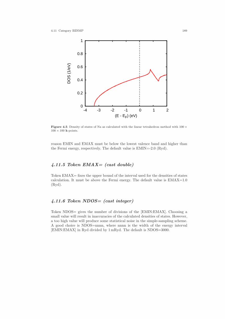
4.11 Category BZSMP 189
0
0.2
0.4
0.6
0.8
1
-4 -3 -2 -1 0 1 2
DO
S (
1/eV
)
(E - EF) (eV)
Figure 4.5 Density of states of Na as calculated with the linear tetrahedron method with 100×100 × 100 k-points.
reason EMIN and EMAX must be below the lowest valence band and higher thanthe Fermi energy, respectively. The default value is EMIN=-2.0 (Ryd).
4.11.5 Token EMAX= (cast double)
Token EMAX= fixes the upper bound of the interval used for the densities of statescalculation. It must be above the Fermi energy. The default value is EMAX=1.0(Ryd).
4.11.6 Token NDOS= (cast integer)
Token NDOS= gives the number of divisions of the [EMIN:EMAX]. Choosing asmall value will result in inaccuracies of the calculated densities of states. However,a too high value will produce some statistical noise in the simple-sampling scheme.A good choice is NDOS=nnnn, where nnnn is the width of the energy interval[EMIN:EMAX] in Ryd divided by 1mRyd. The default is NDOS=3000.

190 4 The main input file: CTRL
4.11.7 Token NORD= (cast integer)
In case that BZINT=HPS has been specified the following two tokens are needed:Token NORD= fixes the order of the approximant in the high-precision Brillouin
zome scheme of Methfessel and Paxton. While low values might cause inaccuracies,high values might lead to too sharp structures. A good choice is NORD=3, whichis the default.
4.11.8 Token WIDTH= (cast double)
This token specifies the internal broadening used for the high-precision Brillouinzome scheme. The default value is WIDTH=0.01 (Ryd).
4.11.9 Token SAVDOS= (cast logical)
Since the calculation of the partial (m-resolved) densities of states (DOS) requiresadditional CPU time, token SAVDOS= has been implemented to switch of calcula-tion of all partial DOS during iteration towards self-consistency. For this reason thedefault is SAVDOS=F. Once full self-consistency is achieved you can choose SAV-DOS=T and calculate the partial densities of states for plotting in one additionalcalculation. It is advantageous to switch from BZINT=SMS to BZINT=HPS in thiscase, too.
4.11.10 Token SAVCOOP= (cast logical)
The meaning of this token is equivalent to that of the previous one. During theiterations, SAVCOOP=F should be used in order to suppress calculation of thecrystal orbital overlap populations (COOP), the crystal orbital Hamiltonian pop-ulation (COHP) or the covalence energy (Ecov) at all. Only in the additional runafter self-consistency has been reached, SAVCOOP=T should be used. Note thatthe latter choice is only effective if the orbitals to be included have been specifiedby tokens COORB= in category CLASS.
4.11.11 Token CTYPE= (cast character)
The token CTYPE= allows to choose the scheme used to describe chemical bonding.At present, it can be either CTYPE=COOP for the crystal orbital overlap popula-

4.11 Category BZSMP 191
tion introduced by Hoffmann [161], CTYPE=COHP for the crystal orbital Hamiltonpopulation as proposed by Dronskowski and Blochl [95], and CTYPE=ECOV forthe covalence energy put forward by Fahnle and coworkers [45, 55, 56].
4.11.12 Token MSPLIT= (cast logical)
This token allows to calculated m-resolved COOP’s. However, this feature has notbeen fully tested and, in addition, requires additional CPU time and memory. Forthese reasons, the default is MSPLIT=F.
4.11.13 Token TEMPFD= (cast double)
With this token you can specify the temperature (in Kelvin) entering the Fermi-Dirac distribution function, which will be used for folding with the calculated densityof states. This allows to evaluate the position of the chemical potential from thecondition that at the given temperature the numbers of excited holes and electronsmust be identical. In a second step these numbers are resolved in contributions fromatoms and angular momenta, i.e. the partial numbers of excited holes and electronsare calculated. This helps to quickly identify the relevant optical transitions. Thedefault is TEMPFD=300 (K).
4.11.14 Token SAVFERM= (cast logical)
With this switch the program is advised to write out information about the Fermisurface for metals, which can be plotted using the XCrysDen software [405]. Thedefault value is SAVFERM=F, which should be used during the self-consistentcalculations. Once full self-consistency is achieved you can choose SAVFERM=T.
4.11.15 Token SAVOPT= (cast logical)
Version 2.4 was the first one, which allowed to calculate the optical conductivity[404]. This includes both the real and imaginary as well as both the absorptive anddispersive parts. As a consequence, no additional Kramers-Kronig transformationis needed. This token can be used to invoke calculation of the optical conductivity.The default value is SAVOPT=F, which should be used during the self-consistentcalculations. Once full self-consistency is achieved you may choose SAVOPT=T.Note that calculation of the optical conductivity is rather time consuming.

192 4 The main input file: CTRL
4.11.16 Token SAVTRAP= (cast logical)
From version 2.6 on, also the calculation of transport properties as based on Boltz-mann theory is implemented. This includes calculation of the electric conductivity,the electronic part of the thermal conductivity, thermopower, the Hall conductiv-ity, and derived quantities [404]. The default value is SAVTRAP=F, which shouldbe used during the self-consistent calculations. Once full self-consistency is achievedyou may choose SAVTRAP=T. Calculation of the transport quantities is somewhattime consuming but the computational demands are considerably lower as for theoptical properties.
4.12 Category CHARGE
4.12.1 Token NETA= (cast integer)
The number of functions per atom and angular momentum to be used to representthe interstitial electron density is fixed to two and cannot be changed on input. Forthis reason, this token is a dummy.
4.12.2 Token EETA= (cast double; length 2)
EETA= is used to specify the energies of the functions used to represent the in-terstitial electron density. The default values are EETA=-3.0 -5.0, which are stillunder consideration. In case you experience instabilities during the iteration processas signaled especially by a negative value for the Fermi energy you should try outswitching to more negative values.
4.12.3 Token SAVRHO= (cast logical)
With this switch you may invoke calculation of the electron densities (core andvalence), their negative Laplacian, and the effective potential. The default value isSAVRHO=F, which should be kept during the self-consistent calculations.
4.13 Category CONTROL 193
4.12.4 Token SAVELF= (cast logical)
In future versions, this switch may be used to invoke calculation of the electronlocalization function and related functions. The default value is SAVELF=F, whichshould be kept during the self-consistent calculations.
4.12.5 Token CHARWIN= (cast logical)
In future versions, this switch will allow to print the electron densities resultingfrom electronic states of only a small energy window as specified by the followingtwo tokens. The default value is CHARWIN=F.
4.12.6 Token EMINC= (cast double)
In future versions, the tokens EMINC= and EMAXC= fix the energy interval usedfor the calculation of the electron densities. The default value is EMINC=-100.0(Ryd).
4.12.7 Token EMAXC= (cast double)
In future versions, token EMAXC= fixes the upper energy limit used for the calcu-lation of the electron densities. The default value is EMAXC=100.0 (Ryd).
4.13 Category CONTROL
4.13.1 Token START= (cast character)
The tokens START= and QUIT= can be used to control the sequence of all cal-culations performed during execution especially of program mnscf.run. In general,ASW calculations towards self-consistency are subdivided into two parts. In onepart, starting from integrals of the partial waves, the program sets up as well asdiagonalizes the secular matrix for every k-point and supplies the local densitymatrices. This part is called the band calculation.
In the other part, the local density matrices are used to calculate electron den-sities, and, using the notions of density functional theory, the potential. The latterin turn allows evaluation of the integrals for use in the secular matrix. This part

194 4 The main input file: CTRL
is called the atomic part. At the start of the program, overlapping atomic electrondensities are used to boot the execution.
In general, four different starting points of the programs execution can be dis-tinguished, which may be selected by token START= but, of course, also dependon the information gained in previous executions.
START=REN Execution starts from scratch. The program performs arenormalized atom calculation using the charges as specifiedby QVAL= and magnetic moments as given by MVAL=, re-spectively. In contrast, if FREE=T has been given, a freeatom calculation is performed using a sphere radius of 20Bohr radii.
START=RST In this case the program does a restart calculation, wherethe local density matrices and the spherically symmetric po-tentials inside the atomic spheres are used to initiate all theatomic calculations. The latter eventually lead to the matrixelements entering the secular matrix.
START=ATM The program invokes one (or more) full band iterations start-ing with the intraatomic calculations, i.e. starting from thelocal density matrices and the spherically symmetric poten-tials inside the atomic spheres in the same manner as for therestart calculations.
START=BND This is the default. The program invokes one or more fullband iterations starting with the Brillouin zone sampling.
In case START= has not been specified the default START=BND will be used.Furthermore the program will look up the atomic files and check them if present.Depending on the outcome of this check the program will then decide automaticallywhere to start. In addition, if START= has been specified, this setting is comparedto the content of the atomic files and the program might opt for a different startingpoint. If, for instance, the atomic sphere radii have been changed in the CTRL-fileand, hence, are no longer in agreement with those given in the atomic files theprogram will automatically invoke a restart calculation. The same happens when achange from a non-spinpolarized to a spinpolarized calculation has been detected.Another case to be mentioned is the situation where START=REN is specified andconverged atomic files exist. In this case the program stops in order to prevent theconverged atomic files from being overwritten.
4.13.2 Token QUIT= (cast character)
Token START= is complemented by token QUIT=, which allows to stop executionprior to the end of the calculation normally performed by the program. To be spe-
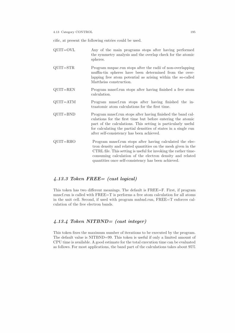
4.13 Category CONTROL 195
cific, at present the following entries could be used.
QUIT=OVL Any of the main programs stops after having performedthe symmetry analysis and the overlap check for the atomicspheres.
QUIT=STR Program mnpac.run stops after the radii of non-overlappingmuffin-tin spheres have been determined from the over-lapping free atom potential as arising within the so-calledMattheiss construction.
QUIT=REN Program mnscf.run stops after having finished a free atomcalculation.
QUIT=ATM Program mnscf.run stops after having finished the in-traatomic atom calculations for the first time.
QUIT=BND Program mnscf.run stops after having finished the band cal-culations for the first time but before entering the atomicpart of the calculations. This setting is particularly usefulfor calculating the partial densities of states in a single runafter self-consistency has been achieved.
QUIT=RHO Program mnscf.run stops after having calculated the elec-tron density and related quantities on the mesh given in theCTRL file. This setting is useful for invoking the rather time-consuming calculation of the electron density and relatedquantities once self-consistency has been achieved.
4.13.3 Token FREE= (cast logical)
This token has two different meanings. The default is FREE=F. First, if programmnscf.run is called with FREE=T is performs a free atom calculation for all atomsin the unit cell. Second, if used with program mnbnd.run, FREE=T enforces cal-culation of the free electron bands.
4.13.4 Token NITBND= (cast integer)
This token fixes the maximum number of iterations to be executed by the program.The default value is NITBND=99. This token is useful if only a limited amount ofCPU time is available. A good estimate for the total execution time can be evaluatedas follows. For most applications, the band part of the calculations takes about 95%

196 4 The main input file: CTRL
of the total execution time. Once the band calculation, i.e. the loop over all k-pointshas started, the program checks the CPU time per k-point and, on adding the CPUtime needed for the previous atomic calculations, prints out the CPU time estimatefor one iteration.
4.13.5 Token CNVG= (cast double)
With this token the desired accuracy of the calculation is fixed. Once this value hasachieved, the self-consistency cycle stops. In particular, CNVG= is the accuracy forthe root mean square difference of the intraatomic charge density resulting fromthe previous and the present iteration. The default value is CNVG=1.0D-8, whichis very accurate. You might well switch to CNVG=1.0D-6 without loosing to much.However, note that going from 10−6 to 10−8 usually requires only very few iterationsand, hence, can be achieved at a very low cost.
4.13.6 Token CNVGET= (cast double)
This token specifies the desired accuracy for the total energy. Whenever the differ-ence between the total energies of the previous and the present iteration is belowthis value, and the condition set by CNVG= is fulfilled, the self-consistency cycleis stopped. The default is CNVGET=1.0D-8 (Ryd), which again is very accurate.
4.13.7 Token NITATM= (cast integer)
Actually, there exist two different self-consistency cycles within the ASW mainprogram mnscf.run. The outer cycle, also called the band iteration, is the usualone, which aims at making the whole electronic density, the effective potential, theHamiltonian matrix etc. self-consistent. In addition, there are intratomic calcula-tions, which are invoked to make a starting electron density from that of overlappingfree atoms. In contrast to token NITBND= the above token NITATM= specifies thenumber of these startup intraatomic iterations. The default value is NITATM=50,which hardly needs a change.
4.13.8 Token CNVGQA= (cast double)
This token fixes the desired accuracy of the intraatomic calculations. Once thisvalue has achieved, the intraatomic self-consistency cycle stops. In particular, CN-

4.14 Category MIXING 197
VGQA= is the accuracy for the root mean square difference of the intraatomicelectron density resulting from the previous and the present intraatomic iteration.The default value is CNVG=1.0D-10, which is very accurate. However, due to thevery low execution time of the intraatomic calculations, this value is well justifiedand needs no changes.
4.14 Category MIXING
This category can be used to influence the iteration towards self-consistency. Actu-ally, there exist two different self-consistency loops. One, which is called the banditeration, affects the calculation of local density matrices once the Brillouin zonesampling has been finished. The other, intraatomic self-consistency loop is per-formed for each atom as part of the intraatomic calculations at startup time of thecalculation in order to construct a starting electron density from those of overlap-ping free atoms. All this is explained in more detail in my review as well as my bookon the ASW method [110,404].
Both types of iterations are accelerated by using the extended Anderson mixing,which superseeds both the elder versions of the Anderson mixing and the Broy-den update [107]. The extended Anderson mixing is controlled by two parameters,namely the number of previous iterations to be mixed in and the mixing parameterβ.
The values proposed for all tokens in this categories have been thoroughly testedin a huge number of applications. They hardly need a change. However, wheneverconvergence is rather slow, you might reduce the β value used for the band iterationsto BETAB=0.3 and switch off the automatic increase of β by setting INCBB=F.
4.14.1 Token NMIXB= (cast integer)
This token holds the number of previous band iterations to be used for the bandmixing. The maximum value is 8, the default is NMIXB=5.
4.14.2 Token BETAB= (cast double)
Here you can specify the mixing parameter to be used for the band mixing. Thedefault is BETAB=0.5.

198 4 The main input file: CTRL
4.14.3 Token INCBB= (cast logical)
With INCBB=T this switch allows to increase the β value used for the band itera-tions, hence, to speedup these iterations once the self-consistency loop has stabilized.
4.14.4 Token NMIXA= (cast integer)
This token holds the number of previous intraatomic iterations to be used for theatomic mixing. The default is NMIXA=5.
4.14.5 Token BETAA= (cast double)
Here you can specify the mixing parameter to be used for the intraatomic mixing.The default is BETAA=0.5.
4.15 Category SUPCELL
4.15.1 Token ALAT= (cast double)
This token contains the supercell lattice constant in the units specified by tokenUNITS=. Default is ALAT=0.0.
4.15.2 Token PLAT= (cast double; length 9)
Information about the Bravais lattice is covered by this token, which contains thethree supercell primitive translations ai, i = 1, 2, 3 in units of the lattice constant.All nine components must be given in the order a1x, a1y , a1z , a2x, a2y, a2z, a3x,a3y, a3z .
4.15.3 Token SLAT= (cast character; marked obsolete)
As an alternative to explicitly specifying the supercell primitive translations byPLAT= you may use the following six tokens, which rely on default lattice vectors

4.15 Category SUPCELL 199
coded in the ASW package. First of all, token SLAT= indicates a string for theBravais lattice. Possible values are
SC: simple cubicBCC: body-centered cubicFCC: face-centered cubicST: simple tetragonalBCT: body-centered tetragonalSO: simple orthorhombicSCO: base-centered orthorhombicBCO: body-centered orthorhombicFCO: face-centered orthorhombicSM: simple monoclinicSCM: base-centered monoclinicTRI: trigonalHEX: hexagonal
Note, however, that the primitive translations coming with these specifications cor-respond to the definitions of Bradley and Cracknell, which in some instances deviatefrom the definitions commonly used. For this reason, you are strongly urged to checkthe primitive translations, which are printed to output at the beginning of the pro-grams execution. Note that the token SLAT= is marked obsolete. Instead the tokenCNTR= should be used.
4.15.4 Token BLAT= (cast double)
For the other lattice constants coming with non-cubic and non-trigonal systemsthere exist two different ways of specification. Token BLAT= gives the lattice con-stant B explicitly in the units specified by token UNITS=. As for ALAT=, thedefault is BLAT=0.0.
4.15.5 Token BBYA= (cast double)
Alternatively, the lattice constant B can be specified by the token BBYA=, whichfixes the ratio of the lattice constants BLAT and ALAT. As for BLAT= above thedefault is BBYA=0.0.

200 4 The main input file: CTRL
4.15.6 Token CLAT= (cast double)
Token CLAT= gives the lattice constant C explicitly in the units specified by tokenUNITS=. As for ALAT=, the default is CLAT=0.0.
4.15.7 Token CBYA= (cast double)
Alternatively, the token CBYA= allows to specify the lattice constant C in termsof the ratio of the lattice constants CLAT and ALAT. The default is CBYA=0.0.
4.15.8 Token ALPHA= (cast double)
With this token the angle between the second and third supercell lattice vectors isspecificed. The default value is ALPHA=90.0.
4.15.9 Token BETA= (cast double)
With this token the angle between the first and third supercell lattice vectors isspecificed. The default value is BETA=90.0.
4.15.10 Token GAMMA= (cast double)
With this token the angle between the first and second supercell lattice vectors isspecificed. The default value is GAMMA=90.0.
4.15.11 Token CNTR= (cast character)
With this token one of the following seven centering types of the supercell Bravaislattice can be specified.
P primitiveC face-centered on the a,b-planeB face-centered on the c,a-planeA face-centered on the b,c-planeI body-centered

4.15 Category SUPCELL 201
F face-centeredR rhombohedral
The default values if CNTR=P.
4.15.12 Token EQUIV= (cast logical)
This switch requires that after construction of the supercell atoms located at theequivalent positions in different subcells still belong to the same class even if theyare not related by a symmetry operation of the supercell. The default is EQUIV=T.
4.15.13 Token CARTS= (cast logical)
This switch specifies whether the following entries for the shift vector are interpretedas Cartesian coordinates (CARTS=T) or as relative components in terms of theprimitive translations (CARTS=F). The default value is CARTS=T.
4.15.14 Token PSHIFT= (cast double; length 3)
This token holds a shift vector, which is added to all atomic positions after a su-percell has been constructed. Note, however, that in order to avoid confusion thistoken is interpreted only by routine mnscl.run. The default is PSHIFT= 0.0 0.0 0.0.
4.15.15 Token CARTQ= (cast logical)
This switch specifies whether the following entries for the spin wave vector areinterpreted as Cartesian coordinates (CARTQ=T) or as relative components interms of the primitive translations (CARTQ=F). The default value is CARTQ=T.

202 4 The main input file: CTRL
4.15.16 Token QSWAVE= (cast double; length 3)
With this token you may specify a spin wave vector for a (collinear) antiferromag-netic structure to be imprinted on the supercell. The simplest case is that of doublingthe unit cell and treating the two subcells as the spin up and spin down sublattice.The spin wave vector must be given in units of 2π divided by the supercell latticeconstant a; its default is QSWAVE= 0.0 0.0 0.0.
4.16 Category SYMLIN
This category comprises all the information needed for plotting the band structure.Note that the program contains a full database of high-symmetry points for allcrystal lattices and all centering types. As a consequence, whenever, the entries forthe high-symmetry points are left empty, they will be taken from the database.
4.16.1 Token NPAN= (cast integer)
This token holds the number of panels, which is the number of different sym-metry lines in the Brillouin zone, along which the band structure is represented.The default is NPAN=0. However, note that for this token the same as for tokensNCLASS= and NBAS= holds. The number of symmetry lines will be calculatedfrom the following entries, but token NPAN= can be used to hide additional entriesfrom the program.
4.16.2 Token NPTS= (cast integer)
Here you can give the maximum number of points to be used for the band structureplot. The actual number will be calculated by the program and usually will beslightly less than the input given by this token. The default is NPTS=400. However,in case you choose to calculate orbital projected band structures (see below), youshould use NPTS=200.
4.16.3 Token ORBWGT= (cast logical)
This switch allows to plot orbital projected band structures. If ORBWGT=T isselected the program will print out the eigenvectors for each k point in addition tothe eigenvalues. This allows to evaluate the contribution from each orbital of the

4.16 Category SYMLIN 203
basis set to the wave function at each k point and for each band, which may berepresented as the width of a bar attached to each E(k) in the plot. The default isORBWGT=F.
4.16.4 Token SPATH= (cast logical)
This switch allows to use spherical pathways for plotting the band structure.For SPATH=T the k-space path will be one the surface of a sphere with radius√Ekin + V0, where Ekin is the kinetic energy of an electron leaving the crystal in
a photoemission experiment and V0 denotes the so-called inner potential. The pathis further specified by the cleavage plane normal vector, which allows to distinguishthe parallel and perpendicular (to the surface) components of the k-vector. Whilethe former is given by
√
h2
2mkin,‖ =
√
h2
2mkout,‖ =
√
Ekin sin(ϑ)
the latter can be calculated from√
h2
2mkin,⊥ =
√
Ekin + V0 −h2
2mk2
in,‖ =√
Ekin cos2(ϑ) + V0
The default is SPATH=F.
4.16.5 Token EKPV0= (cast double)
With this token the value of√Ekin + V0, i.e. the radius of the sphere in k-space is
specified. The default value is EKPV0=0.0.
4.16.6 Token CPNORM= (cast double; length 3)
With this token the cleavage plane is specified, which allows to distinguish theparallel and perpendicular (to the surface) components of the k-vector. By default,all components of the cleavage plane normal vector are set to zero.
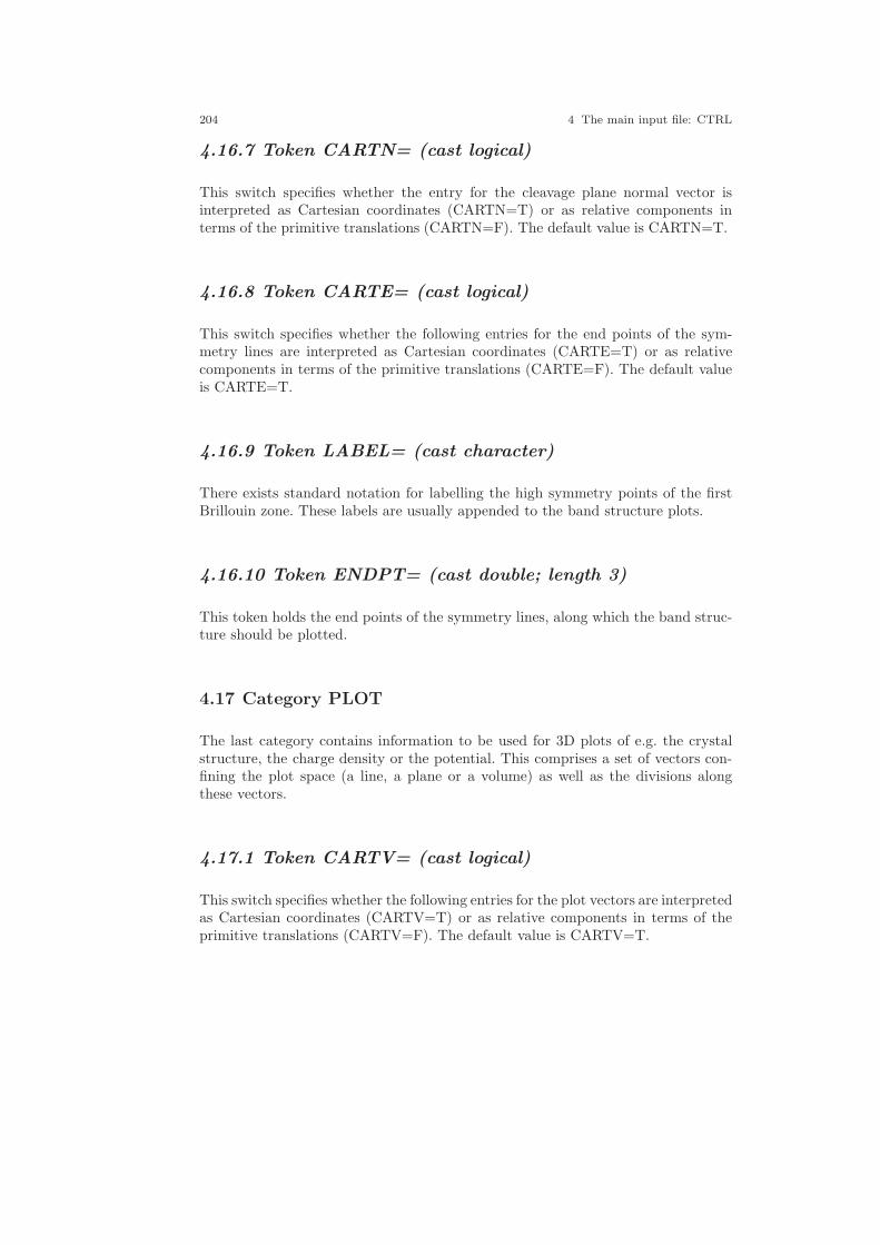
204 4 The main input file: CTRL
4.16.7 Token CARTN= (cast logical)
This switch specifies whether the entry for the cleavage plane normal vector isinterpreted as Cartesian coordinates (CARTN=T) or as relative components interms of the primitive translations (CARTN=F). The default value is CARTN=T.
4.16.8 Token CARTE= (cast logical)
This switch specifies whether the following entries for the end points of the sym-metry lines are interpreted as Cartesian coordinates (CARTE=T) or as relativecomponents in terms of the primitive translations (CARTE=F). The default valueis CARTE=T.
4.16.9 Token LABEL= (cast character)
There exists standard notation for labelling the high symmetry points of the firstBrillouin zone. These labels are usually appended to the band structure plots.
4.16.10 Token ENDPT= (cast double; length 3)
This token holds the end points of the symmetry lines, along which the band struc-ture should be plotted.
4.17 Category PLOT
The last category contains information to be used for 3D plots of e.g. the crystalstructure, the charge density or the potential. This comprises a set of vectors con-fining the plot space (a line, a plane or a volume) as well as the divisions alongthese vectors.
4.17.1 Token CARTV= (cast logical)
This switch specifies whether the following entries for the plot vectors are interpretedas Cartesian coordinates (CARTV=T) or as relative components in terms of theprimitive translations (CARTV=F). The default value is CARTV=T.
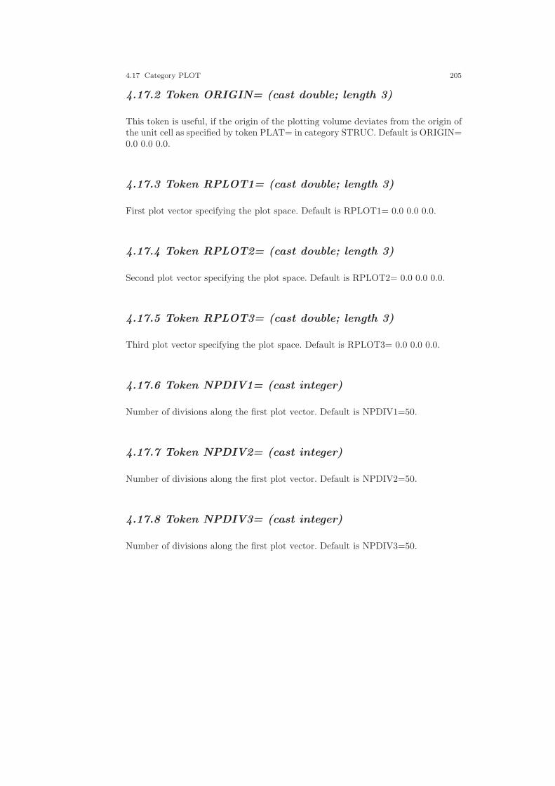
4.17 Category PLOT 205
4.17.2 Token ORIGIN= (cast double; length 3)
This token is useful, if the origin of the plotting volume deviates from the origin ofthe unit cell as specified by token PLAT= in category STRUC. Default is ORIGIN=0.0 0.0 0.0.
4.17.3 Token RPLOT1= (cast double; length 3)
First plot vector specifying the plot space. Default is RPLOT1= 0.0 0.0 0.0.
4.17.4 Token RPLOT2= (cast double; length 3)
Second plot vector specifying the plot space. Default is RPLOT2= 0.0 0.0 0.0.
4.17.5 Token RPLOT3= (cast double; length 3)
Third plot vector specifying the plot space. Default is RPLOT3= 0.0 0.0 0.0.
4.17.6 Token NPDIV1= (cast integer)
Number of divisions along the first plot vector. Default is NPDIV1=50.
4.17.7 Token NPDIV2= (cast integer)
Number of divisions along the first plot vector. Default is NPDIV2=50.
4.17.8 Token NPDIV3= (cast integer)
Number of divisions along the first plot vector. Default is NPDIV3=50.

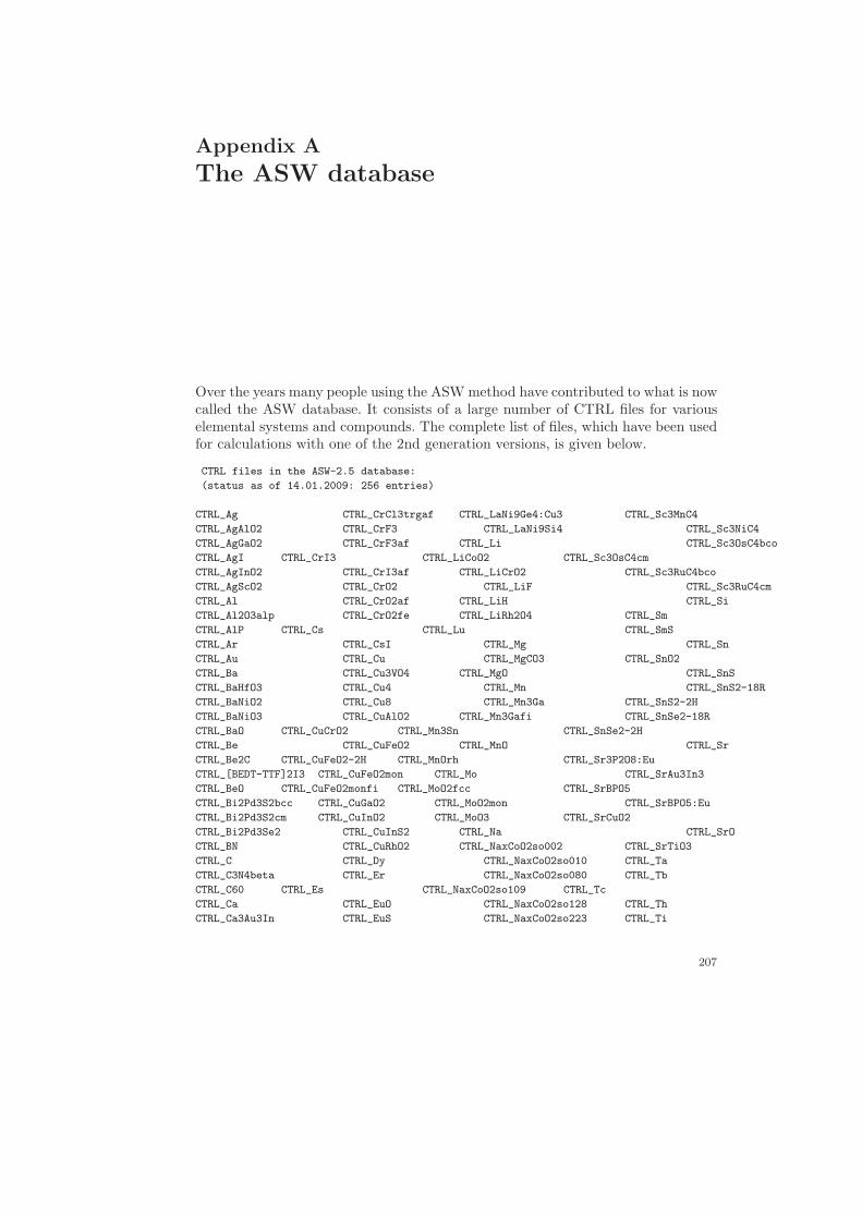
Appendix A
The ASW database
Over the years many people using the ASW method have contributed to what is nowcalled the ASW database. It consists of a large number of CTRL files for variouselemental systems and compounds. The complete list of files, which have been usedfor calculations with one of the 2nd generation versions, is given below.
CTRL files in the ASW-2.5 database:
(status as of 14.01.2009: 256 entries)
CTRL_Ag CTRL_CrCl3trgaf CTRL_LaNi9Ge4:Cu3 CTRL_Sc3MnC4
CTRL_AgAlO2 CTRL_CrF3 CTRL_LaNi9Si4 CTRL_Sc3NiC4
CTRL_AgGaO2 CTRL_CrF3af CTRL_Li CTRL_Sc3OsC4bco
CTRL_AgI CTRL_CrI3 CTRL_LiCoO2 CTRL_Sc3OsC4cm
CTRL_AgInO2 CTRL_CrI3af CTRL_LiCrO2 CTRL_Sc3RuC4bco
CTRL_AgScO2 CTRL_CrO2 CTRL_LiF CTRL_Sc3RuC4cm
CTRL_Al CTRL_CrO2af CTRL_LiH CTRL_Si
CTRL_Al2O3alp CTRL_CrO2fe CTRL_LiRh2O4 CTRL_Sm
CTRL_AlP CTRL_Cs CTRL_Lu CTRL_SmS
CTRL_Ar CTRL_CsI CTRL_Mg CTRL_Sn
CTRL_Au CTRL_Cu CTRL_MgCO3 CTRL_SnO2
CTRL_Ba CTRL_Cu3VO4 CTRL_MgO CTRL_SnS
CTRL_BaHfO3 CTRL_Cu4 CTRL_Mn CTRL_SnS2-18R
CTRL_BaNiO2 CTRL_Cu8 CTRL_Mn3Ga CTRL_SnS2-2H
CTRL_BaNiO3 CTRL_CuAlO2 CTRL_Mn3Gafi CTRL_SnSe2-18R
CTRL_BaO CTRL_CuCrO2 CTRL_Mn3Sn CTRL_SnSe2-2H
CTRL_Be CTRL_CuFeO2 CTRL_MnO CTRL_Sr
CTRL_Be2C CTRL_CuFeO2-2H CTRL_MnOrh CTRL_Sr3P2O8:Eu
CTRL_[BEDT-TTF]2I3 CTRL_CuFeO2mon CTRL_Mo CTRL_SrAu3In3
CTRL_BeO CTRL_CuFeO2monfi CTRL_MoO2fcc CTRL_SrBPO5
CTRL_Bi2Pd3S2bcc CTRL_CuGaO2 CTRL_MoO2mon CTRL_SrBPO5:Eu
CTRL_Bi2Pd3S2cm CTRL_CuInO2 CTRL_MoO3 CTRL_SrCuO2
CTRL_Bi2Pd3Se2 CTRL_CuInS2 CTRL_Na CTRL_SrO
CTRL_BN CTRL_CuRhO2 CTRL_NaxCoO2so002 CTRL_SrTiO3
CTRL_C CTRL_Dy CTRL_NaxCoO2so010 CTRL_Ta
CTRL_C3N4beta CTRL_Er CTRL_NaxCoO2so080 CTRL_Tb
CTRL_C60 CTRL_Es CTRL_NaxCoO2so109 CTRL_Tc
CTRL_Ca CTRL_EuO CTRL_NaxCoO2so128 CTRL_Th
CTRL_Ca3Au3In CTRL_EuS CTRL_NaxCoO2so223 CTRL_Ti
207
208 A The ASW database
CTRL_Ca3Ru2O7ht CTRL_Fe CTRL_NaxCoO2so300 CTRL_Ti2O3ht
CTRL_Ca3Ru2O7lt CTRL_Fe2 CTRL_NaxCoO2so450 CTRL_Ti2O3rt
CTRL_CaCu3Ru4O12 CTRL_Fe4 CTRL_Nb CTRL_TiB
CTRL_CaNiN CTRL_Fe8 CTRL_NbO CTRL_TiO
CTRL_CaO CTRL_FeC24S2N6 CTRL_NbSe2-2H CTRL_TiO2ant
CTRL_CaTe2O5 CTRL_FeS2 CTRL_Nd CTRL_TiO2rut
CTRL_Cd CTRL_Ga2O3 CTRL_Ne CTRL_TiSi2fco
CTRL_CdCr2S4 CTRL_GaN CTRL_[NH2CH2COOH]2*HNO3 CTRL_TiSi2sco
CTRL_CdS CTRL_GaP CTRL_Ni CTRL_TiTe2
CTRL_Ce CTRL_Gd CTRL_Ni2MnGa CTRL_Tl
CTRL_Ce2RuZn4 CTRL_GdN CTRL_NiS CTRL_TlI
CTRL_CeNi9Ge4 CTRL_GdS CTRL_NiSisc CTRL_Tm
CTRL_CeNi9Ge4:Cu1 CTRL_Ge CTRL_NiSiso CTRL_U
CTRL_CeNi9Ge4:Cu2 CTRL_H CTRL_Os CTRL_UB2
CTRL_CeNi9Ge4:Cu3 CTRL_He CTRL_OsS2 CTRL_UB4
CTRL_CeNi9Si4 CTRL_Hf CTRL_Pb CTRL_UB6
CTRL_CeRhSn CTRL_Hg CTRL_Pd CTRL_UO2
CTRL_CeRuSn CTRL_Ho CTRL_PdCoO2 CTRL_V
CTRL_CH3ReO3 CTRL_In CTRL_Pr CTRL_VH
CTRL_CN2 CTRL_In2O3 CTRL_PrRuSn CTRL_VO
CTRL_Co2MnGe CTRL_In2VO5 CTRL_Pt CTRL_W
CTRL_Co2O3hs CTRL_In2VO5af CTRL_PtCoO2 CTRL_Xe
CTRL_Co2O3ls CTRL_InP CTRL_Pu CTRL_Y
CTRL_Co3In2S2 CTRL_Ir CTRL_Rb CTRL_Yb
CTRL_CoO CTRL_IrO2rut CTRL_Re CTRL_YB6
CTRL_CP2 CTRL_K CTRL_Rh CTRL_YF3
CTRL_Cr CTRL_KB6 CTRL_RhO2 CTRL_YFe2
CTRL_Cr2F5 CTRL_Kr CTRL_Ru CTRL_Zn
CTRL_CrBr3 CTRL_La CTRL_RuC CTRL_ZnCr2Se4
CTRL_CrBr3af CTRL_LaBaCo2O55 CTRL_RuS2 CTRL_ZnO
CTRL_CrCl2 CTRL_LaCoO3 CTRL_Sc CTRL_ZnS
CTRL_CrCl2af CTRL_LaMnO3so CTRL_Sc3C4 CTRL_ZnV2O4ht
CTRL_CrCl3 CTRL_LaNi9Ge4 CTRL_Sc3CoC4 CTRL_ZnV2O4lt
CTRL_CrCl3af CTRL_LaNi9Ge4:Cu1 CTRL_Sc3FeC4 CTRL_Zr
CTRL_CrCl3trg CTRL_LaNi9Ge4:Cu2 CTRL_Sc3FeC4af CTRL_ZrFe2
In addition, there exist a lot of CTRL files, which are still in the format used bythe 1st generation version and have not yet been transformed. However, they wouldbe fully compatible with the 2nd generation programs.
Whenever you want to perform a calculation for one of the systems already in thedatabase just copy the CTRL file. However, please read the README file containedin the database before. In turn, I do welcome any new CTRL file.

Appendix B
Brillouin zones
This Appendix displays the Brillouin zones of some lattices.
...................................................................................................................................................................................................................................................................................................................................................................................................................................................................................................................................... ............................................................................................................................................................................................................................................................................................................................................................................... .............................................................................................................................................................................................................................................................................................................
........................................................................................................................................................................................................ .............................................................................................................................................................................................................................................................................................................................................................................................................................................................................................................................................................................................................................................................................................................................................................................................................................................................................................................................................................................................................................................................................................................................................................................................................................................................................................................................................................................................................................................................................................................................................................................................................................................................................................................................................................................................................................................................................................................................................................................................................................................................................................................................................................................................................................................................................................................................................................................................................................................................................................................................................................................................................................................................................................................................................................................................................................................................................................................................................................................................................................................................................................................................................................................................................................................................................................................................................................................................................................................................................................................................................................................................................................................................................................................................................................................................................................................................................................................................................................................................................................................
..............................................................................................................................................................................................................................................................................................................
.............................................................................................................................................................................................................................................................................................................
............................................................................................................................................................................................................................................................................................................................................................................................................................................................................................................................................................................................................................................................................................................................................................................................................................................................................................................................................................................................................................................................................u u uu
kx kykz
� M XR
(a) simple cubic
...................................................................................................................................................................................................................................................................................................................................................................................................................................................................................................................................... ............................................................................................................................................................................................................................................................................................................................................................................... .............................................................................................................................................................................................................................................................................................................
........................................................................................................................................................................................................ .............................................................................................................................................................................................................................................................................................................................................................................................................................................................................................................................................................................................................................................................................................................................................................................................................................................................................................................................................................................................................................................................................................................................................................................................................................................................................................................................................................................................................................................................................................................................................................................................................................................................................................................................................................................................................................................................................................................................................................................................................................................................................................................................................................................................................................................................................................................................................................................................................................................................................................................................................................................................................................................................................................................................................................................................................................................................................................................................................................................................................................................................................................................................................................................................................................................................................................................................................................................................................................................................................................................................................................................................................................................................................................................................................................................................................................................................................................................................................................................................................................................
..............................................................................................................................................................................................................................................................................................................
.............................................................................................................................................................................................................................................................................................................
.....................................................................................................................................................................................................................................................................................................................................................................................................................................................................................................................................................................................................................................................................................................................................................................................................................................................................................................................................................................................................................................................................................................................................................................................................................................................................................................................................................................................................................................................................................................................................................................................................................................................................................................................................................................................................................................................................u u uu
ukx kykz
� M XR
X0(b) T 6
hstructure
........................................................................................................................................................................................................................................................................................................................................................................................................................ ..................................................................................................................................................................................................................................................................................................................................................................................................................................... ............................................................................................................................................................................................................................................................................................................
....................................................................................... ....................................................................................................................................................................................................................................................................................................................................................................................................................................................................................................................................................................................................................................................................................................................................................................................................................................................................................................................................................................................................................................................................................................................................................................................................................................................................................................................................................................................................................................................................................................................................................................................................................................................................................................................................................................................................................................................................................................................................................................................................... ............................................................................................................................................................................................................................................................................................................................................................................................................................................................................................................................................................................................................................................................................................................................................................................................................................................................................................................................................................................................................................................................................................................................................................................... ............................................................................................................................................................................................................................................................................................................................................................................................................................................................................................................................................................................................................................................................................................................................................................................................................................................................................................................................................................................................................u u u uu ukx ky
kz� K W XL U
(c) face-centered cubic
........................................................................................................................................................................................................................................................................................................................................................................................................................ ..................................................................................................................................................................................................................................................................................................................................................................................................................................... .............................................................................................................................................................................................................................................................................................................
...................................................................................... .......................................................................................................................................................................................................................................................................................................................................................................................................................................................................................................................................................................................................................................................................................................................................................................................................................................................................................................................................................................................................................................................................................................................................................................................................................................................................................................................................................................................................................................................................................................................................................................................................................................................................................................................................................................................................................................................................................................................................................................................................................................................................................................................................................................................................................................................................................................................................................................................................................
.............................................................................................................................................................................................................................................................................................................................................................................................................................................................................................................................................................................................................................................................................................................................................................................................................................................................................................................................................................................................................................................................................................................................................................................u uu ukx kykz� NP H
(d) body-centered cubic
Figure B.1 Brillouin zones of cubic lattices.
209
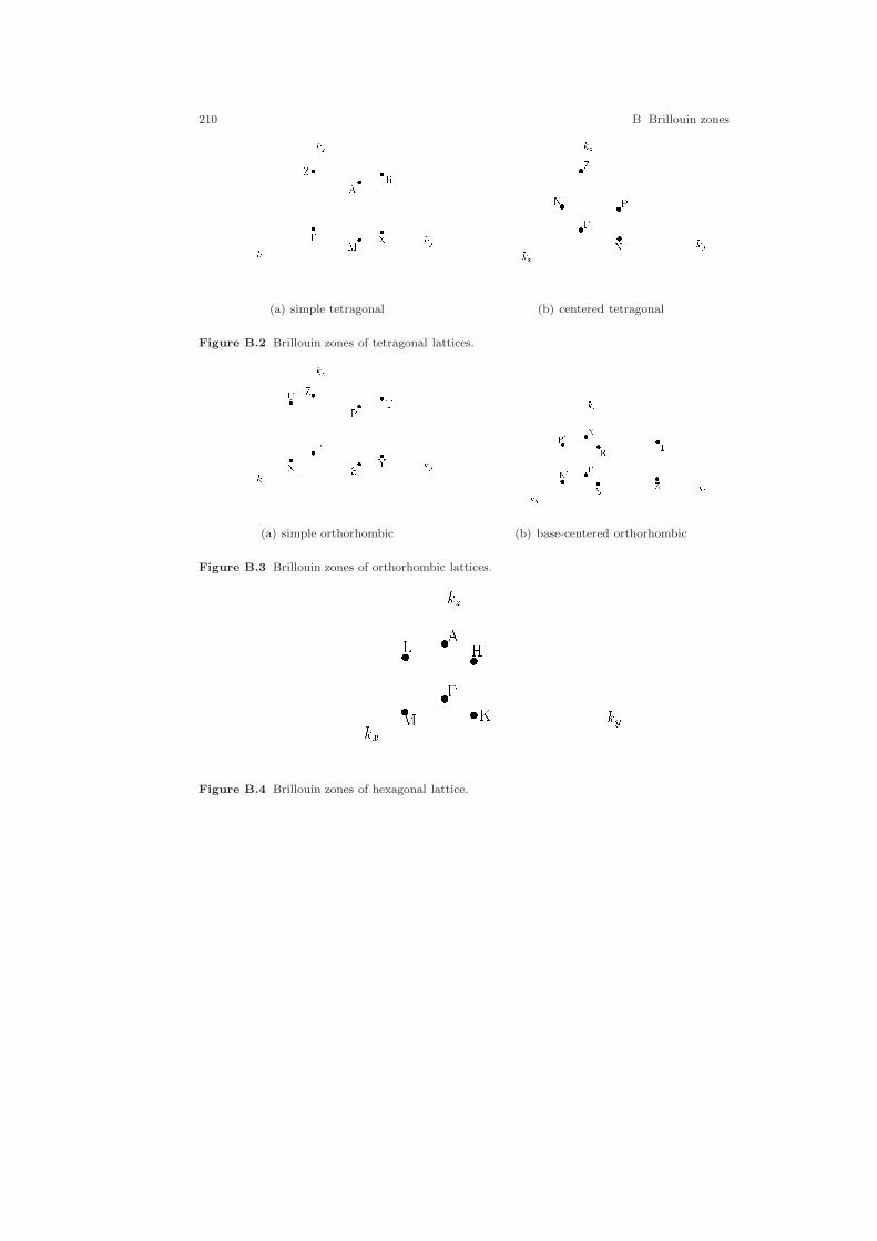
210 B Brillouin zones
................................................................................................................................................................................................................................................................................................................................................................................................................................................................................................................... ............................................................................................................................................................................................................................................................................................................................................................................... ............................................................................................................................................................................................................................................................................................................
................................................................................................................ .................................................................................................................................................................................................................................................................................................................................................................................................................................................................................................................................................................................................................................................................................................................................................................................................................................................................................................................................................................................................................................................................................................................................................................................................................................................................................................................................................................................................................................................................................................................................................................................................................................................................................................................................................................................................................................................................................................................................................................................................................................................................................................................................................................................................................................................................................................................................................................................................................................................................................................................................................................................................................................................................................................................................................................................................................................................................................................................................................................................................................................................................................................................................................................................................................................................................................................................................................................................................................................................................................................................................................................................................................................................................................................................................. .............................................................................................................................................................................................................................................................................................................
...................................................................................................................................................................................................................................................................................................................................................................................................................................................................................................................................................................................................................................................................................................................................... uu uuuukx kykz�Z RXMA
(a) simple tetragonal
............................................................................................................................................................................................................................................................................................................................................................................................................................................. ............................................................................................................................................................................................................................................................................................................................. ............................................................................................................................................................................................................................................................................................................................................................................................................................................................................................................................................................................................................................................................................................................................................................................................................................................................................................................................................................................................................................................................................................................................................................................................................................................................................................................................................................................................................................................................................................................................................................................................................................................................................................................................................................................................................................................................................................................................................................................................................................................................................................................................................................................................................................................................................................................................................................................................................................................................................................................................................................................. ........................................................................................................................................................................................................................................................................................................................................................... ............................................................................................................................................................................................................................................................................................................................................................................................................................... ........................................................................................................................................................................................................................................................................................................................................................................................................................................................................................................................................................................................................................................................................................................ ........................................................................................................................................................................................................................................................................................................................................................ uu uuukx kykz�Z XPN
(b) centered tetragonal
Figure B.2 Brillouin zones of tetragonal lattices.
................................................................................................................................................................................................................................................................................................................................................................................................................................................................................................................... ............................................................................................................................................................................................................................................................................................................................................................................... ............................................................................................................................................................................................................................................................................................................
................................................................................................................ ................................................................................................................................................................................................................................................................................................................................................................................................................................................................................................................................................................................................................................................................................................................................................................................................................................................................................................................................................................................................................................................................................................................................................................................................................................................................................................................................................................................................................................................................................................................................................................................................................................................................................................................................................................................................................................................................................................................................................................................................................................................................................................................................................................................................................................................................................................................................................................................................................................................................................................................................................................................................................................................................................................................................................................................................................................................................................................................................................................................................................................................................................................................................................................................................................................................................................ .................................................................................................................................................................................................................................................................................................................................................................................................................................................................................................................................................................................................................................................................................................................................................................................................................................................................................................................................................................................................................................................................................................................................................................................................................................................... ............................................................................................................................................................................................................................................................................................................
.................................................................................................................................................................uu uuuuuukx kykz�Z TYSRXU
(a) simple orthorhombic
..................................................................................................................................................................................................................................................................................................................................................................................................................................................................................................................... ................................................................................................................................................................................................................................................................................................................................................................... ....................................................................................................................................................................................................................................................................................................................................................................... .................................................................................................................................................................................................................................................................................................................................................................................................................................................................................................................................................................................................................................................................................................................................................................................................................................................................................................................................................................................................................................................................................................................................................................................................................................................................................................................................................................................................................................................................................................................................................................................................................................................................................................................................................................................................................................................
............................................................................................................................................................................................................................................................................................................................................................................................................................................................................................................................................................................................................................................................................................................................................................................................................................................................................................................................................................................................................................................................................................................................................................................................................................................................................................................................................................................................................................................................................................................................................................................................................................
......................................................................................................................................................................................................................................................................................................................................................................................................................................................................................................................................................................................................................................................................................................................................................................................................................................................................................................................................................................... ...................................................................................................................................................uu uuuuuu kxky kz�X TZSRN0P0
(b) base-centered orthorhombic
Figure B.3 Brillouin zones of orthorhombic lattices......................................................................................................................................................................................................................................................................................................................................................................................................................... .................................................................................................................................................................................................................................................................................................................. .............................................................................................................................................................................................................................................................................................................. .............................................................................................................................................................................................................................................................................................................................................................................................................................................................................................................................................................................................................................................................................................................................................................................................................................................................................................................................................................................................................................................................................................................................................................................................................................................................................................................................................................................................................................................................................................................................................................................................................................................................................................................................................................................................................................................................................................................................................................................................................................................................................................................................................................................................................................................................................................................................................................................................................................................................................................................................................................................................................................................................................................................................................................................................................................................................................................................................................................................................................................................................................................................................................................................................................................................................................................................................................................................................................................uuuu uukx kykz�ALM KHFigure B.4 Brillouin zones of hexagonal lattice.
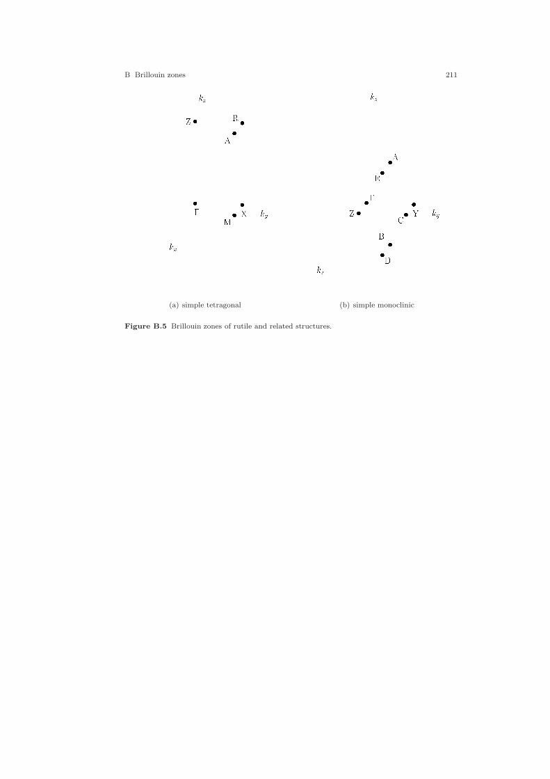
B Brillouin zones 211
.............................................................................................................................................................................................................................................................................................. .......................................................................................................................................................................................................................................................................................................................................................... ...................................................................................................................................................................................................................................................................................................................................................
........................................................................................................................................................................................................................................... .......................................................................................................................................................................................................................................................................................................................................................................................................................................................................................................................................................................................................................................................................................................................................................................................................................................................................................................................................................................................................................................................................................................................................................................................................................................................................................................................................................................................................................................................................................................................................................................................................................................................................................................................................................................................................................................................................................................................................................................................................................................................................................................................................................................................................................................................................................................................................................................................................................................................................................................................................................................................................................................................................................................................................................................................................................................................................................................................................................................................................................................................................................................................................................................................................................................................................................................................................................................................................................................................................................................................................................................................................................................................................................................................................................................................................................................................................................................................................................................................................................................................................................................................
..............................................................................................................................................................................................................................................................................................................
...............................................................................................................................................................................................................................................................................................................................................................................................................................................................................................................................................................................................................................................................................................................................................................................................................................................................................................................................................................................................................................................................................................................................................................................................................................................................................................................................................................................................................................................................................
....................................................................................................................................................................................................................uu
uu
uu
kx kykz�
ZX
RMA
(a) simple tetragonal
....................................................................................................................................................................................................................................................................................................................................................................................................... .......................................................................................................................................................................................................................................................................................................................................................... ..................................................................................................................................................................................................................................................................................................................................................
............................................................................................................................................................................................................................................ ......................................................................................................................................................................................................................................................................................................................................................................................................................................................................................................................................................................................................................................................................................................................................................................................................................................................................................................................................................................................................................................................................................................................................................................................................................................................................................................................................................................................................................................................................................................................................................................................................................................................................................................................................................................................................................................................................................................................................................................................................................................................................................................................................................................................................................................................................................................................................................................................................................................................................................................................................................................................................................................................................................................................................................................................................................................................................................................................................................................................................................................................................................................................................................................................................................................................................................................................................................................................................................................................................................................................................................................................................................................................................................................................................................................................................................................................................................................................................................................................................................................................................................................................
.............................................................................................................................................................................................................................................................................................................
.............................................................................................................................................................................
................................................................................................................................................................................................................................................................................................................................................................................................................................................................................................................................................................................................................................................................................................................................................................................................................................................................................................................................................................................................................................................................................................................................................................................................................................................................................................................................................
............................................................................................................................................................................................................................................................................................................................................................................................................................................................................................................................................................................................................................................................................................................................................................................................................................................................................................................................................................................................................................................................................................................................................................................................................................................................................................................................................................................................................................................................................................................................................................................................................................................................................................................................................................................................................................................................................ .......................................................................................................... .......................................................................................................... ..........................................................................................................
.................................................................................................................................................................................................................... ............................................................................................................................................................................................................................................................................................................................................................................................................................................................................................................................................................................................................................................................................................................................................................................................................................................................................................................................................................................................................................................................................................................................................................................................................................................................................................................................................................................................................................. .....................................................uu uuuu uukx ky
kz�Z YCAEBD
(b) simple monoclinic
Figure B.5 Brillouin zones of rutile and related structures.

References
1. M. Abramowitz and I. A. Stegun, Handbook of Mathematical Functions (Dover, New York1972)
2. H. Akai and P. H. Dederichs, J. Phys. C 18, 2455 (1985)3. P. B. Allen, Boltzmann theory and resistivity of metals. In: Quantum Theory of Real Mate-
rials, ed by J. R. Chelikowsky and S. G. Louie (Kluwer, Boston 1996) pp 219–2504. C. Ambrosch-Draxl and J. O. Sofo, Comput. Phys. Commun. 175, 1 (2006)5. D. E. Amos, ACM Trans. Math. Software 6, 365 (1980)6. D. E. Amos, ACM Trans. Math. Software 6, 420 (1980)7. D. E. Amos, ACM Trans. Math. Software 9, 467 (1983)8. D. E. Amos, ACM Trans. Math. Software 9, 525 (1983)9. O. K. Andersen, Comments on the KKR-Wavefunction; Extension of the Spherical Wave
Expansion beyond the Muffin-Tins. In: Computational Methods in Band Theory, ed byP. M. Marcus, J. F. Janak, and A. R. Williams (Plenum Press, New York 1971) pp 178–182
10. O. K. Andersen, Solid State Commun. 13, 133 (1973)11. O. K. Andersen, Phys. Rev. B 12, 3060 (1975)12. O. K. Andersen, Linear Methods in Band Theory. In: The Electronic Structure of Complex
Systems, ed by P. Phariseau and W. Temmerman (Plenum Press, New York 1984) pp 11–6613. O. K. Andersen, Muffin-Tin Orbital Theory. Lecture Notes from the ICTP workshop on
Methods on Electronic Structure Calculations, (International Center for Theoretical Physics,Trieste 1992)
14. O. K. Andersen and O. Jepsen, Phys. Rev. Lett. 53, 2571 (1984)15. O. K. Andersen, O. Jepsen, and D. Glotzel, Canonical Description of the Band Structures of
Metals. In: Highlights of Condensed-Matter Theory, Proceedings of the International Schoolof Physics “Enrico Fermi”, Course LXXXIX, ed by F. Bassani, F. Fumi, and M. P. Tosi(North-Holland, Amsterdam 1985) pp 59–176
16. O. K. Andersen, O. Jepsen, and G. Krier, Exact Muffin-Tin Orbital Theory. In: Methods
of Electronic Structure Calculations, ed by V. Kumar, O. K. Andersen, and A. Mookerjee(World Scientific, Singapore 1994) pp 63–124
17. O. K. Andersen, O. Jepsen, and M. Sob, Linearized Band Structure Methods. In: Electronic
Band Structure and its Applications, ed by M. Yussouff (Springer, Berlin 1986) pp 1–5718. O. K. Andersen and R. V. Kasowski, Phys. Rev. B 4, 1064 (1971)19. O. K. Andersen and R. V. Kasowski, Solid State Commun. 11, 799 (1972)20. O. K. Andersen, Z. Pawlowska, and O. Jepsen, Phys. Rev. B 34, 5253 (1986)21. O. K. Andersen, A. P. Postnikov, and S. Yu. Savrasov, The Muffin-Tin Orbital Point of View.
In: Applications of Multiple Scattering Theory to Materials Science, ed by W. H. Butler,P. H. Dederichs, A. Gonis, and R. L. Weaver, Mat. Res. Soc. Symp. Proc. 253, 37 (1992)
22. O. K. Andersen, H. L. Skriver, H. Nohl, and B. Johansson, Pure Appl. Chem. 52, 93 (1979)
213

214 References
23. O. K. Andersen and R. G. Woolley, Mol. Phys. 26, 905 (1973)24. D. G. Anderson, J. Assoc. Comput. Mach. 12, 547 (1965)25. V. I. Anisimov, F. Aryasetiawan, and A. I. Liechtenstein, J. Phys.: Condens. Matter 9, 767
(1997)26. V. I. Anisimov and O. Gunnarsson, Phys. Rev. B 43, 7570 (1991)27. V. I. Anisimov, I. V. Solovyev, M. A. Korotin, M. T. Czyzyk and G. A. Sawatzky,
Phys. Rev. B 48, 16929 (1993)28. V. I. Anisimov, J. Zaanen, and O. K. Andersen, Phys. Rev. B 44, 943 (1991)29. V. N. Antonov, P. M. Oppeneer, A. N. Yaresko, A. Y. Perlov, and T. Kraft, Phys. Rev. B
56, 13012 (1997)30. N. W. Ashcroft and N. D. Mermin, Solid State Physics (Holt-Saunders, Philadelphia 1976)31. K. Atkinson, J. Austral. Math. Soc. B 23, 332 (1982)32. R. F. W. Bader and P. M. Beddall, J. Chem. Phys. 56, 3320 (1972)33. A. Baldereschi, Phys. Rev. B 7, 5212 (1973)34. U. von Barth, Density-Functional Theory for Solids. In: The Electronic Structure of Complex
Systems, ed by P. Phariseau and W. Temmerman (Plenum Press, New York 1984) pp 67–14035. U. von Barth, An Overview of Density-Functional Theory. In: Many-Body Phenomena at
Surfaces, ed by D. Langreth and H. Suhl (Academic Press, Orlando 1984) pp 3–5036. U. von Barth, Different Approximations Within Density-Functional Theory, Their Advan-
tages and Limitations. In: Methods of Electronic Structure Calculations, ed by V. Kumar,O. K. Andersen, and A. Mookerjee (World Scientific, Singapore 1994) pp 21–62
37. U. von Barth and L. Hedin, J. Phys. C 5, 1629 (1972)38. U. von Barth and A. Pedroza, Phys. Scr. 32, 353 (1985)39. Z. P. Bazant and B. H. Oh, Z. Angew. Math. Mech. 66, 37 (1986)40. A. D. Becke, Phys. Rev. A 38, 3098 (1988)41. A. D. Becke, J. Chem. Phys. 98, 5648 (1993)42. A. D. Becke and K. E. Edgecombe, J. Chem. Phys. 92, 5397 (1990)43. P. Bendt and A. Zunger, Phys. Rev. B 26, 3114 (1982)44. C. L. Berman and L. Greengard, J. Math. Phys. 35, 6036 (1994)45. G. Bester and M. Fahnle, J. Phys.: Cond. Matt. 13, 11541 (2001)46. F. Birch, Phys. Rev. 47, 809 (1947)47. M. A. Blanco, M. Florez, and M. Bermejo, J. Mol. Struct. (Theochem) 419, 19 (1997)48. F. Bloch, Z. Phys. 52, 555 (1929)49. P. E. Blochl, Gesamtenergien, Krafte und Metall-Halbleiter Grenzflachen. PhD thesis, Uni-
versitat Stuttgart (1989)50. P. E. Blochl, Phys. Rev. B 50, 17953 (1994)51. P. E. Blochl, O. Jepsen, and O. K. Andersen, Phys. Rev. B 49, 16223 (1994)52. S. Blugel, First Principles Calculations of the Electronic Structure of Magnetic Overlayers on
Transition Metal Surfaces. PhD thesis, Rheinisch-Westfalische Technische Hochschule Aachen(1987)
53. M. Born and M. Bradburn, Proc. Cambridge Phil. Soc. 39, 104 (1943)54. M. Born and R. Oppenheimer, Ann. Phys. (Leipzig) 84, 457 (1927)55. N. Bornsen, G. Bester, B. Meyer, and M. Fahnle, J. Alloys Comp. 308, 1 (2000)56. N. Bornsen, B. Meyer, O. Grotheer, and M. Fahnle, J. Phys.: Cond. Matt. 11, L287 (1999)57. L. P. Bouckaert, R. Smoluchowski, and E. P. Wigner, Phys. Rev. 50, 58 (1936)58. C. J. Bradley and A. P. Cracknell, The Mathematical Theory of Symmetry in Solids (Claren-
don Press, Oxford 1972)59. R. P. Brent, Algorithms for Minimization without Derivatives (Prentice Hall, Englewood
Cliffs 1973)60. M. S. S. Brooks and P. J. Kelly, Phys. Rev. Lett. 51, 1708 (1983)61. C. G. Broyden, Math. Comput. 19, 577 (1965)62. C. G. Broyden, Math. Comput. 21, 368 (1966)63. K. Burke, J. P. Perdew, and M. Ernzerhof, J. Chem. Phys. 109, 3760 (1998)64. G. D. Byrne and C. A. Hall, Numerical Solution of Systems of Nonlinear Algebraic Equations
(Academic Press, New York, London 1973)

References 215
65. J. Callaway, Energy Band Theory (Academic Press, New York 1964)66. J. Callaway, Quantum Theory of the Solid State (Academic Press, Boston 1991)67. J. Callaway and N. H. March, Density-Functional Methods: Theory and Applications. In:
Solid State Physics vol 38, ed by F. Seitz, D. Turnbull, and H. Ehrenreich (Academic Press,Orlando 1983) pp 136–223
68. R. Car and M. Parrinello, Phys. Rev. Lett. 55, 2471 (1985)69. R. Car and M. Parrinello, Phys. Rev. Lett. 60, 204 (1988)70. F. Casula and F. Herman, J. Chem. Phys. 78, 858 (1983)71. D. M. Ceperley, Phys. Rev. B 18, 3126 (1978)72. D. M. Ceperley and B. J. Alder, Phys. Rev. Lett. 45, 566 (1980)73. D. J. Chadi, Phys. Rev. B 16, 1746 (1977)74. D. J. Chadi and M. L. Cohen, Phys. Rev. B 8, 5747 (1973)75. J. P. A. Charlesworth and W. Yeung, Comput. Phys. Commun. 88, 186 (1995)76. J. Chen, J. B. Krieger, Y. Li, and G. J. Iafrate, Phys. Rev. A 54, 3939 (1996)77. C. Chiccoli, S. Lorenzutta, and G. Maino, J. Comput. Phys. 78, 278 (1988)78. C. Chiccoli, S. Lorenzutta, and G. Maino, Computing 45, 269 (1990)79. C. H. Choi, J. Ivanic, M. S. Gordon, and K. Rudenberg, J. Chem. Phys. 111, 8825 (1999)80. N. E. Christensen, Phys. Rev. B 29, 5547 (1984)81. H. J. H. Clercx and P. P. J. M. Schram, J. Math. Phys. 34, 5292 (1993)82. M. H. Cohen and F. Reif, Quadrupole Effects in Nuclear Magnetic Resonance Studies of
Solids. In: Solid State Physics, vol 5, ed by F. Seitz and D. Turnbull (Academic Press,Orlando 1970) pp 321–438
83. P. T. Coleridge, J. Molenaar, and A. Lodder, J. Phys. C 15, 6943 (1982)84. P. Cortona, S. Doniach, and C. Sommers, Phys. Rev. B 31, 2842 (1985)85. G. Czycholl, Theoretische Festkorperphysik, (Springer, Berlin 2004)86. M. T. Czyzyk and G. A. Sawatzky, Phys. Rev. B 49, 14211 (1995)87. M. Danos and L. C. Maximon, J. Math. Phys. 6, 766 (1965)88. P. H. Dederichs and R. Zeller, Phys. Rev. B 28, 5462 (1983)89. F. M. F. de Groot, J. C. Fuggle, B. T. Thole, and G. A. Sawatzky, Phys. Rev. B 42, 5459
(1990)90. J. E. Dennis, Jr., and J. J. More, SIAM Review 19, 46 (1977)91. H.-Q. Ding, N. Karasawa, and W. A. Goddard, Chem. Phys. Lett. 196, 6 (1992)92. J. F. Dobson, J. Chem. Phys. 94, 4328 (1991)93. R. M. Dreizler and E. K. U. Gross, Density-Functional Theory (Springer, Berlin 1990)94. R. M. Dreizler and J. de Providencia, Density-Functional Methods in Physics (Plenum Press,
New York 1985)95. R. Dronskowski and P. E. Blochl, J. Phys. Chem. 97, 8617 (1993)96. K. J. Duff, Int. J. Quant. Chem. 5, 111 (1971)97. H. Ebert, Rep. Prog. Phys. 59, 1665 (1996)98. N. Elyashar and D. D. Koelling, Phys. Rev. B 13, 5362 (1976)99. E. Engel and S. H. Vosko, Phys. Rev. B 47, 2800 (1993)
100. E. Engel and S. H. Vosko, Phys. Rev. B 47, 13164 (1993)101. E. Engel and S. H. Vosko, Phys. Rev. B 50, 10498 (1994)102. H. Eschrig, Optimized LCAO Method and the Electronic Structure of Extended Systems
(Springer, Berlin 1989)103. H. Eschrig, The Fundamentals of Density-Functional Theory (Edition am Gutenbergplatz,
Leipzig 2003)104. P. P. Ewald, Ann. Phys. 49, 1 (1916)105. P. P. Ewald, Ann. Phys. 64, 253 (1921)106. V. Eyert, Entwicklung und Implementation eines Full-Potential-ASW-Verfahrens. PhD the-
sis, Technische Hochschule Darmstadt (1991)107. V. Eyert, J. Comput. Phys. 124, 271 (1996)108. V. Eyert, Electronic structure calculations for crystalline materials. In: Density-Functional
Methods: Applications in Chemistry and Materials Science, ed by M. Springborg (Wiley,Chichester 1997) pp 233–304

216 References
109. V. Eyert, Octahedral Deformations and Metal-Insulator Transition in Transition MetalChalcogenides. Habilitation thesis, University of Augsburg (1998)
110. V. Eyert, Basic notions and applications of the augmented spherical wave method,Int. J. Quantum Chem. 77, 1007 (2000)
111. V. Eyert, Electronic Structure of Crystalline Materials, 2nd edn (University of Augsburg,Augsburg 2005)
112. V. Eyert and K.-H. Hock, Phys. Rev. B 57, 12727 (1998)113. R. Feder, F. Rosicky, and B. Ackermann, Z. Phys. 52, 31 (1983)114. B. U. Felderhof and R. B. Jones, J. Math. Phys. 28, 836 (1987)115. L. G. Ferreira, J. Comput. Phys. 36, 198 (1980)116. R. P. Feynman, Phys. Rev. 56, 340 (1939)
117. G. E. Forsythe and C. B. Moler, Computer Solution of Linear Algebraic Systems (PrenticeHall, Englewood Cliffs 1967); Computer-Verfahren fur lineare algebraische Systeme (Olden-bourg, Munchen 1971)
118. D. L. Foulis, J. Math. Phys. 34, 2004 (1993)119. L. Fritsche and J. Yuan, Phys. Rev. A 57, 3425 (1998)120. S. Froyen, Phys. Rev. B 39, 3168 (1989)121. K. Fuchs, Proc. Roy. Soc. A 151, 585 (1935)122. E. R. Fuller and E. R. Naimon, Phys. Rev. B 6, 3609 (1972)123. R. Gaspar, Acta Phys. Hung. 3, 263 (1954)124. W. Gautschi, SIAM Rev. 9, 24 (1967)125. W. Gautschi, Commun. ACM 12, 635 (1969)126. W. Gautschi, SIAM J. Numer. Anal. 7, 187 (1970)127. W. Gautschi, ACM Trans. Math. Software 5, 466 (1979)128. W. Gautschi, ACM Trans. Math. Software 5, 482 (1979)129. C. D. Gelatt, Jr., H. Ehrenreich, and R. E. Watson, Phys. Rev. B 15, 1613 (1977)130. D. K. Ghosh, Phys. Rev. Lett. 27, 1584 (1971)131. G. Gilat and N. R. Bharatiya, Phys. Rev. B 12, 3479 (1975)132. S. Goedecker, Phys. Rev. B 48, 17573 (1993)133. D. E. Goldberg, Genetic Algorithms in Search, Optimization, and Machine Learning
(Addison-Wesley, Reading 1989)134. H. Gollisch and L. Fritsche, phys. stat. sol. (b) 86, 145 (1978)135. A. Gonis, Phys. Rev. B 33, 5914 (1986)136. A. Gorling, Phys. Rev. A 47, 2783 (1993)137. A. Gorling, Phys. Rev. B 53, 7024 (1996)138. A. Gorling and M. Levy, Phys. Rev. A 50, 196 (1994)139. I. S. Gradshteyn and I. M. Ryzhik, Table of Integrals, Series and Products (Academic Press,
New York 1980)140. E. K. U. Gross and R. M. Dreizler, Density-Functional Theory (Plenum Press, New York
1995)141. O. Gunnarsson, J. Phys. F 6, 587 (1976)142. O. Gunnarsson, J. Harris, and R. O. Jones, Phys. Rev. B 15, 3027 (1977)143. O. Gunnarsson, J. Harris, and R. O. Jones, J. Chem. Phys. 67, 3970 (1977)144. O. Gunnarsson and R. O. Jones, Phys. Rev. B 31, 7588 (1985)145. O. Gunnarsson and B. I. Lundqvist, Phys. Rev. B 13, 4274 (1976)146. O. Gunnarsson, B. I. Lundqvist, and J. W. Wilkins, Phys. Rev. B 10, 1319 (1974)147. D. Hackenbracht, Berechnete elektronische und thermomechanische Eigenschaften einiger
La-In und Al-Ni - Verbindungen. Diploma thesis, Ruhr-Universitat Bochum (1979)148. F. S. Ham and B. Segall, Phys. Rev. 124, 1786 (1961)149. J. Hama and M. Watanabe, J. Phys.: Cond. Matt. 4, 4583 (1992)150. J. Hama, M. Watanabe, and T. Kato, J. Phys.: Cond. Matt. 2, 7445 (1990)151. A. Haug, Theoretical Solid State Physics (Pergamon Press, New York 1972)152. J. Harris, Phys. Rev. B 31, 1770 (1985)153. J. Harris and G. S. Painter, Phys. Rev. B 22, 2614 (1980)

References 217
154. J. Harris, Density-Functional Calculations for Atomic Clusters. In: The Electronic Structure
of Complex Systems, ed by P. Phariseau and W. Temmerman (Plenum Press, New York1984) pp 141–182
155. W. A. Harrison, Electronic Structure and the Properties of Solids (Freeman, San Fransisco1980)
156. L. Hedin, Phys. Rev. 139, A796 (1965)157. L. Hedin and B. I. Lundqvist, J. Phys. C 4, 2064 (1971)158. V. Heine, Electronic Structure from the Point of View of the Local Atomic Environment. In:
Solid State Physics, vol 35, ed by H. Ehrenreich, F. Seitz, and D. Turnbull (Academic Press,New York 1980) pp 1–127
159. D. M. Heyes, Phys. Lett. A 187, 273 (1994)
160. L. Hodges, R. E. Watson, H. Ehrenreich, Phys. Rev. B 5, 3953 (1972)161. R. Hoffmann, Solids and Surfaces: A Chemist’s View of Bonding in Extended Structures
(VCH Verlagsgesellschaft, New York 1988)162. P. Hohenberg and W. Kohn, Phys. Rev. 136, B864 (1964)163. G. Hummer, Chem. Phys. Lett. 235, 297 (1995)164. J. Ivanic and K. Rudenberg, J. Phys. Chem. 100, 6342 (1996)165. A. Jablonski, J. Comput. Phys. 111, 256 (1994)166. J. D. Jackson, Classical Electrodynamics (Wiley, New York 1975)167. D. A. H. Jacobs, The State of the Art in Numerical Analysis (Academic Press, London 1977)168. J. F. Janak, Phys. Rev. B 9, 3985 (1974)169. J. F. Janak, V. L. Moruzzi, and A. R. Williams, Phys. Rev. B 12, 1257 (1975)170. O. Jepsen and O. K. Andersen, Solid State Commun. 9, 1763 (1971)171. O. Jepsen and O. K. Andersen, Phys. Rev. B 29, 5965 (1984)172. O. Jepsen, O. K. Andersen, and A. R. Mackintosh, Phys. Rev. B 12, 3084 (1975)173. O. Jepsen, J. Madsen, and O. K. Andersen, Phys. Rev. B 26, 2790 (1982)174. O. Jepsen and O. K. Andersen, Z. Phys. B 97, 35 (1995)175. D. D. Johnson, Phys. Rev. B 38, 12807 (1988)176. R. O. Jones and O. Gunnarsson, Rev. Mod. Phys. 61, 689 (1989)177. R. Jones and A. Sayyash, J. Phys. C 19, L653 (1986)178. W. Jones and N. H. March, Theoretical Solid State Physics (Wiley, London 1973)179. S. Kaprzyk and P. E. Mijnarends, J. Phys. C 19, 1283 (1986)180. R. V. Kasowski, Phys. Rev. B 25, 4189 (1982)181. R. V. Kasowski, M.-H. Tsai, T. N. Rhodin, and D. D. Chambliss, Phys. Rev. B 34, 2656
(1986)182. P. Keast, J. Comput. Appl. Math. 17, 151 (1987)183. P. Keast and J. C. Diaz, SIAM J. Numer. Anal. 20, 406 (1983)184. J. Keller, J. Phys. C 4, L85 (1971)185. G. P. Kerker, Phys. Rev. B 23, 3082 (1981)186. C. Kittel, Introduction to Solid State Physics (Wiley, New York 1986)187. C. Kittel, Quantum Theory of Solids (Wiley, New York, 1987)188. L. Kleinman, Phys. Rev. B 28, 1139 (1983)189. J. Kohler, Polarer, magneto-optischer Kerr-Effekt in kollinear und nicht-kollinear magnetis-
chen, metallischen Verbindungen. PhD thesis, Technische Universitat Darmstadt (1998)190. D. D. Koelling, J. Comput. Phys. 67, 253 (1986)191. D. D. Koelling and G. O. Arbman, J. Phys. F 5, 2041 (1975)192. D. D. Koelling and B. N. Harmon, J. Phys. C 10, 3107 (1977)193. W. Kohn and N. Rostoker, Phys. Rev. 94, 1111 (1954)194. W. Kohn and L. J. Sham, Phys. Rev. 140, A1133 (1965)195. W. Kohn and P. Vashishta, General Density-Functional Theory. In: Theory of the Inhomo-
geneous Electron Gas, ed by S. Lundqvist and N. H. March (Plenum Press, New York 1983)pp 79–147
196. J. Korringa, Physica 13, 392 (1947)197. J. Korringa, Phys. Rep. 238, 341 (1994)

218 References
198. G. F. Koster, Space Groups and Their Representations. In: Solid State Physics, vol 5, ed byF. Seitz and D. Turnbull (Academic Press, Orlando 1970) pp 173–256
199. T. Kotani, Phys. Rev. B 50, 14816 (1994)200. T. Kotani, Phys. Rev. Lett. 74, 2989 (1995)201. T. Kotani and H. Akai, Phys. Rev. B 52, 17153 (1995)202. T. Kotani and H. Akai, Phys. Rev. B 54, 16502 (1996)203. O. V. Kovalev, Irreducible Representations of Space Groups (Gordon and Breach, New York
1965)204. A. Kratzer and W. Franz, Transzendente Funktionen (Akademische Verlagsgesellschaft,
Leipzig 1960)205. G. Kresse and J. Furthmuller, Phys. Rev. B 54, 11169 (1996)206. J. B. Krieger, Y. Li, and G. J. Iafrate, Phys. Lett. A 146, 256 (1990)207. J. B. Krieger, Y. Li, and G. J. Iafrate, Phys. Lett. A 148, 470 (1990)208. J. B. Krieger, Y. Li, and G. J. Iafrate, Phys. Rev. A 45, 101 (1992)209. J. B. Krieger, Y. Li, and G. J. Iafrate, Phys. Rev. A 46, 5453 (1992)210. B. C. H. Krutzen and F. Springelkamp, J. Phys.: Cond. Matt. 1, 8369 (1989)211. E. S. Kryachko, E. V. Ludena, Energy Density-Functional Theory of Many-Electron Systems
(Kluwer Academic Publishers, Dordrecht 1990)212. J. Kubler and V. Eyert, Electronic structure calculations. In: Electronic and Magnetic Prop-
erties of Metals and Ceramics, ed by K. H. J. Buschow (VCH Verlagsgesellschaft, Weinheim1992) pp 1–145;vol 3A of Materials Science and Technology, ed by R. W. Cahn, P. Haasen, and E. J. Kramer(VCH Verlagsgesellschaft, Weinheim 1991-1996)
213. J. Kubler, K.-H. Hock, J. Sticht, and A. R. Williams, J. Phys. F 18, 469 (1988)214. J. Kubler, K.-H. Hock, J. Sticht, and A. R. Williams, J. Appl. Phys. 63, 3482 (1988)215. R. Kutteh, E. Apra, and J. Nichols, Chem. Phys. Lett. 238, 173 (1995)216. P. Lambin and P. Senet, Int. J. Quant. Chem. 46, 101 (1993)217. P. Lambin and J. P. Vigneron, Phys. Rev. B 29, 3430 (1984)218. W. R. L. Lambrecht and O. K. Andersen, Phys. Rev. B 34, 2439 (1986)219. D. A. Langs, J. Appl. Cryst. 29, 481 (1996)220. F. Lechermann, Ab-initio Betrachtungen zur Elektronenstruktur und Statistischen Mechanik
von mehrkomponentigen intermetallischen Systemen am Beispiel Ni-Fe-Al. PhD thesis, Uni-versity of Stuttgart (2003)
221. G. Lehmann, phys. stat. sol. 38, 151 (1970)222. G. Lehmann, P. Rennert, M. Taut, and H. Wonn, phys. stat. sol. 37, K27 (1970)223. G. Lehmann and M. Taut, phys. stat. sol. (b) 54, 469 (1972)224. H. van Leuken, Electronic Structure of Metallic Multilayers. PhD thesis, University of Ams-
terdam (1991)225. M. Levy, Proc. Natl. Acad. Sci. (USA) 76, 6062 (1979)226. M. Levy, Phys. Rev. A 26, 1200 (1982)227. M. Levy and J. P. Perdew, Phys. Rev. B 48, 11638 (1993)228. M. Levy and J. P. Perdew, Int. J. Quant. Chem. 49, 539 (1994)229. Y. Li, J. B. Krieger, M. R. Norman, and G. J. Iafrate, Phys. Rev. B 44, 10437 (1991)230. A. I. Liechtenstein, V. I. Anisimov, and J. Zaanen, Phys. Rev. B 52, R5467 (1995)231. E. H. Lieb, Int. J. Quant. Chem. 24, 243 (1983)232. P. O. Lowdin, Adv. Phys. 5, 1 (1956)233. T. Loucks, Augmented Plane Wave Method (Benjamin, New York 1967)234. W. Ludwig, Festkorperphysik (Akad. Verlagsgesellschaft, Heidelberg 1970)235. W. Ludwig and C. Falter, Symmetries in Physics (Springer, Berlin 1996)236. S. Lundqvist and N. H. March, Theory of the Inhomogeneous Electron Gas (Plenum Press,
New York 1983)237. A. H. MacDonald, J. Phys. C 16, 3869 (1983)238. A. H. MacDonald, W. E. Pickett, and D. D. Koelling, J. Phys. C 13, 2675 (1980)239. A. H. MacDonald and S. H. Vosko, J. Phys. C 12, 2977 (1979)240. A. H. MacDonald, S. H. Vosko, and P. T. Coleridge, J. Phys. C 12, 2991 (1979)

References 219
241. A. R. Mackintosh and O. K. Andersen, The electronic structure of transition metals In:Electrons at the Fermi Surface, ed by M. Springford (University Press, Cambridge 1980)pp 149–224
242. J. M. MacLaren, D. P. Clougherty, and R. C. Albers, Phys. Rev. B 42, 3205 (1990)243. J. M. MacLaren, D. P. Clougherty, M. E. McHenry, and M. M. Donovan, Comput. Phys. Com-
mun. 66, 383 (1991)244. G. K. H. Madsen and D. J. Singh, Comput. Phys. Commun. 175, 67 (2006)245. W. Magnus, F. Oberhettinger, and R. P. Soni, Formulas and Theorems for the Special Func-
tions of Mathematical Physics (Springer, Berlin 1966)246. G. D. Mahan and J. O. Sofo, Proc. Natl. Acad. Sci. USA 93, 7436 (1996)247. P. M. Marcus, J. F. Janak, and A. R. Williams, Computational Methods in Band Theory
(Plenum Press, New York 1971)248. L. F. Mattheiss, Phys. Rev. 133, A1399 (1964)249. L. F. Mattheiss and D. R. Hamann, Phys. Rev. B 33, 823 (1986)250. T. Maurer, Berechnung des magneto-optischen Kerr-Effekts. Diploma thesis, Technische
Hochschule Darmstadt (1991)251. A. D. McLaren, Math. Comput. 17, 361 (1963)252. A. Messiah, Quantum Mechanics, vol 1 (North Holland, Amsterdam 1976)253. A. Messiah, Quantum Mechanics, vol 2 (North Holland, Amsterdam 1978)254. M. S. Methfessel, Zur Berechnung der Losungswarme von Metallhydriden. Diploma thesis,
Ruhr-Universitat Bochum (1980)255. M. S. Methfessel, Multipole Green Functions for Electronic Structure Calculations. PhD
thesis, University of Nijmegen (1986)256. M. S. Methfessel, Phys. Rev. B 38, 1537 (1988)257. M. S. Methfessel and J. Kubler, J. Phys. F 12, 141 (1982)258. M. S. Methfessel and A. T. Paxton, Phys. Rev. B 40, 3616 (1989)259. M. S. Methfessel, C. O. Rodriguez, and O. K. Andersen, Phys. Rev. B 40, 2009 (1989)260. M. S. Methfessel and M. van Schilfgaarde, Phys. Rev. B 48, 4937 (1993)261. M. S. Methfessel, M. van Schilfgaarde, and R. A. Casali, A full-Potential LMTO Method
Based on Smooth Hankel Functions. In: Electronic Structure and Physical Properties of
Solids. The Uses of the LMTO Method, ed by H. Dreysse (Springer, Berlin, Heidelberg,2000) pp 114–147
262. M. S. Methfessel, M. van Schilfgaarde, and M. Scheffler, Phys. Rev. Lett. 70, 29 (1993)263. M. S. Milgram, Math. Comput. 44, 443 (1985)264. R. D. Misra, Proc. Cambridge Phil. Soc. 36, 173 (1940)265. H. J. Monkhorst and J. D. Pack, Phys. Rev. B 13, 5188 (1976)266. P. M. Morse and H. Feshbach, Methods of Theoretical Physics (McGraw-Hill, New York
1953)267. V. L. Moruzzi, J. F. Janak, and A. R. Williams, Calculated Electronic Properties of Metals
(Pergamon Press, New York 1978)268. I. P. Mysovskih, Sov. Math. Dokl. 18, 925 (1977)269. F. D. Murnaghan, Am. J. Math. 49, 235 (1937)270. F. D. Murnaghan, Proc. Nat. Acad. Sci. 30, 244 (1944)271. B. R. Nag, Electron Transport in Compounds Semiconductors, (Springer, Berlin 1980)272. A. Nagy, Phys. Rev. A 55, 3465 (1997)273. V. Natoli and D. M. Ceperley, J. Comput. Phys. 117, 171 (1995)274. W. Nolting, Grundkurs: Theoretische Physik, vol 3: Elektrodynamik (Springer, Berlin 2004)275. W. Nolting, Grundkurs: Theoretische Physik, vol 5, part 1: Quantenmechanik – Grundlagen
(Springer, Berlin, 2004)276. H. J. Nowak, O. K. Andersen, T. Fujiwara, O. Jepsen, and P. Vargas, Phys. Rev. B 44, 3577
(1991)277. R. Nozawa, J. Math. Phys. 7, 1841 (1966)278. P. M. Oppeneer and A. Lodder, J. Phys. F 17, 1885 (1987)279. P. M. Oppeneer, J. Sticht, and F. Herman, J. Magn. Soc. Jpn. 15, Suppl. S1, 73 (1991)280. P. M. Oppeneer, T. Maurer, J. Sticht, and J. Kubler, Phys. Rev. B 45, 10924 (1992)

220 References
281. P. M. Oppeneer, J. Sticht, T. Maurer, and J. Kubler, Z. Phys. B 88, 309 (1992)282. J. M. Ortega and W. C. Rheinboldt, Iterative Solution of Nonlinear Equations in Several
Variables (Academic Press, New York 1970)283. H. Ou-Yang and M. Levy, Phys. Rev. Lett. 65, 1036 (1994)284. G. S. Painter, Phys. Rev. B 24, 4264 (1981)285. D. A. Papaconstantopoulos, Handbook of the Band Structure of Elemental Solids (Plenum
Press, New York 1986)286. R. G. Parr and W. Yang, Density-Functional Theory of Atoms and Molecules (Oxford Uni-
versity Press, Oxford 1989)287. J. P. Perdew, Phys. Rev. B 33, 8822 (1986)288. J. P. Perdew, Physica B 172, 1 (1991)
289. J. P. Perdew, Unified Theory of Exchange and Correlation Beyond the Local Density Approx-imation. In: Electronic Structure of Solids ’91, ed by P. Ziesche and H. Eschrig (AkademieVerlag, Berlin 1991) pp 11–20
290. J. P. Perdew, K. Burke, and M. Ernzerhof, Phys. Rev. Lett. 77, 3865 (1996)291. J. P. Perdew, K. Burke, and M. Ernzerhof, Phys. Rev. Lett. 80, 891 (1998)292. J. P. Perdew, K. Burke, and Y. Wang, Phys. Rev. B 54, 16533 (1996)293. J. P. Perdew, J. A. Chevary, S. H. Vosko, K. A. Jackson, M. R. Pederson, D. J. Singh, and
C. Fiolhais, Phys. Rev. B 46, 6671 (1992)294. J. P. Perdew and M. Levy, Phys. Rev. Lett. 51, 1884 (1983)295. J. P. Perdew and Y. Wang, Phys. Rev. B 33, 8800 (1986)296. J. P. Perdew and Y. Wang, Phys. Rev. B 45, 13244 (1992)297. J. P. Perdew and A. Zunger, Phys. Rev. B 23, 5048 (1981)298. H. G. Petersen, D. Soelvason, J. W. Perram, and E. R. Smith, J. Chem. Phys. 101, 8870
(1994)299. A. G. Petukhov, I. I. Mazin, L. Chioncel, and A. I. Liechtenstein, Phys. Rev. B 67, 153106
(2003)300. C. J. Pickard and M. C. Payne, Phys. Rev. B 59, 4685 (1999)301. W. E. Pickett, H. Krakauer, and P. B. Allen, Phys. Rev. B 38, 2721 (1988)302. E. Polak, Computational Methods in Optimization (Academic Press, New York 1971)303. E. L. Pollock and J. Glosli, Comput. Phys. Commun. 95, 93 (1996)304. G. P. M. Poppe and C. M. J. Wijers, ACM Trans. Math. Software 16, 38 (1990)305. A. S. Popov, Comput. Math. Math. Phys. 35, 369 (1995)306. M. Posternak, H. Krakauer, A. J. Freeman, and D. D. Koelling, Phys. Rev. B 21, 5601 (1980)307. W. H. Press, B. P. Flannery, S. A. Teukolsky, and W. T. Vetterling, Numerical Recipes –
The Art of Scientific Computing (Cambridge University Press, Cambridge 1989)308. D. L. Price and B. R. Cooper, Phys. Rev. B 39, 4945 (1989)309. P. Pulay, Mol. Phys. 17, 197 (1969)310. P. Pulay, Mol. Phys. 18, 473 (1970)311. P. Pulay, Chem. Phys. Lett. 73, 393 (1980)312. P. Pulay and F. Torok, Mol. Phys. 25, 1153 (1973)313. A. K. Rajagopal, J. Phys. C 11, L943 (1978)314. A. K. Rajagopal, Adv. Chem. Phys. 41, 59 (1980)315. A. K. Rajagopal and J. Callaway, Phys. Rev. B7, 1912 (1973)316. G. Rajagopal and R. J. Needs, J. Comput. Phys. 115, 399 (1994)317. M. V. Ramana and A. K. Rajagopal, J. Phys. C 12, L845 (1979)318. M. V. Ramana and A. K. Rajagopal, Adv. Chem. Phys. 54, 231 (1983)319. M. Rasolt and D. J. W. Geldart, Phys. Rev. B 34, 1325 (1986)320. J. Rath and A. J. Freeman, Phys. Rev. B 11, 2109 (1975)321. H. W. A. M. Rompa, R. Eppenga, and M. F. H. Schuurmans, Physica 145B, 5 (1987)322. M. E. Rose, Elementary Theory of Angular Momentum (Wiley, New York 1957)323. M. E. Rose, Relativistic Electron Theory (Wiley, New York 1961)324. A. Savin, A. D. Becke, J. Flad, R. Nesper, H. Preuß, and H. G. von Schnering,
Angew. Chem. 103, 421 (1991); Angew. Chem. Int. Ed. Engl. 30, 409 (1991)

References 221
325. A. Savin, O. Jepsen, J. Flad, O. K. Andersen, H. Preuß, and H. G. von Schnering,Angew. Chem. 104, 186 (1992)
326. S. Y. Savrasov and D. Y. Savrasov, Phys. Rev. B 46, 12181 (1992)327. T. J. Scheidemantel, C. Ambrosch-Draxl, T. Thonhauser, J. V. Badding, and J. O. Sofo,
Phys. Rev. B 68, 125210 (2003)328. W. W. Schulz, P. B. Allen, and N. Trivedi, Phys. Rev. B 45, 10886 (1992)329. B. Segall and F. S. Ham, In: Methods in Computational Physics, ed by B. Alder, S. Fernbach,
and M. Rotenberg (Academic Press, New York 1968) pp 251–293330. A. Seidl, A. Gorling, P. Vogl, J. A. Majewski, and M. Levy, Phys. Rev. B 53, 3764 (1996)331. W. F. Shadwick, J. D. Talman, and M. R. Norman, Comput. Phys. Commun. 54, 95 (1989)332. L. J. Sham and M. Schluter, Phys. Rev. Lett. 51, 1888 (1983)333. R. T. Sharp and G. K. Horton, Phys. Rev. 90, 317 (1953)334. A. B. Shick, A. I. Liechtenstein, and W. E. Pickett, Phys. Rev. B 60, 10763 (1999)335. C. A. Sholl, Proc. Phys. Soc. 91, 130 (1967)336. C. A. Sholl, Proc. Phys. Soc. 92, 434 (1967)337. R. Sinclair and F. Ninio, J. Phys.: Cond. Matt. 2, 2143 (1990)338. D. J. Singh, Planewaves, Pseudopotentials and the LAPW Method (Kluwer Academic Pub-
lishers, Boston 1994)339. D. Singh, H. Krakauer, and C. S. Wang, Phys. Rev. B 34, 8391 (1986)340. H. L. Skriver, The LMTO Method (Springer, Berlin 1984)341. J. C. Slater, Phys. Rev. 51, 846 (1937)342. A. P. Smith and N. W. Ashcroft, Phys. Rev. B 38, 12942 (1988)343. J. Soler and A. R. Williams, Phys. Rev. B 40, 1560 (1989)344. J. Soler and A. R. Williams, Phys. Rev. B 42, 9728 (1990)345. J. Soler and A. R. Williams, Phys. Rev. B 47, 6784 (1993)346. I. V. Solovyev, P. H. Dederichs, and V. I. Anisimov, Phys. Rev. B 50, 16861 (1994)347. M. Springborg and O. K. Andersen, J. Chem. Phys. 87, 7125 (1987)348. M. Springborg, Density-Functional Methods: Applications in Chemistry and Materials Sci-
ence, (Wiley, Chichester 1997)349. G. P. Srivastava, J. Phys. A 17, L317 (1984)350. G. P. Srivastava and D. Weaire, Adv. Phys. 36, 463 (1987)351. M. Stadele, J. A. Majewski, P. Vogl, and A. Gorling, Phys. Rev. Lett. 79, 2089 (1997)352. J. Sticht, Bandstrukturrechnung fur Schwere-Fermionen-Systeme. PhD thesis, Technische
Hochschule Darmstadt (1989)353. J. Sticht, K.-H. Hock, and J. Kubler, J. Phys.: Cond. Matt. 1, 8155 (1989)354. J. Stoer, Numerische Mathematik 1, (Springer, Berlin 1993)355. P. Strange, J. Staunton, B. L. Gyorffy, J. Phys. C 17, 3355 (1984)356. A. H. Stroud, Approximate Calculation of Multiple Integrals (Prentice-Hall, Englewood Cliffs
1971)357. A. H. Stroud, SIAM J. Numer. Anal. 10, 559 (1973)358. H. Takayama, M. Tsukuda, H. Shiba, F. Yonezawa, M. Imada, and Y. Okabe, Computational
Physics as a New Frontier in Condensed Matter Research (The Physical Society of Japan,Tokyo 1995)
359. T. Takeda, Z. Phys. B 32, 43 (1978)360. T. Takeda, J. Phys. F 9, 815 (1979)361. T. Takeda, J. Phys. F 10, 1135 (1980)362. J. D. Talman, Comput. Phys. Commun. 54, 85 (1989)363. J. D. Talman and W. F. Shadwick, Phys. Rev. A 14, 36 (1976)364. M. Taut, Phys. Rev. B 57, 2217 (1998)365. M. P. Tosi, Cohesion of Ionic Solids in the Born Model. In: Solid State Physics, vol 16, ed
by F. Seitz and D. Turnbull (Academic Press, New York 1964) pp 1–120366. A. Y. Toukmaji and J. A. Board, Jr., Comput. Phys. Commun. 95, 73 (1996)367. D. Vanderbilt and S. G. Louie, Phys. Rev. B 30, 6118 (1984)368. G. Vignale and M. Rasolt, Phys. Rev. Lett. 59, 2360 (1987)369. G. Vignale and M. Rasolt, Phys. Rev. B 37, 10685 (1988)

222 References
370. S. H. Vosko, L. Wilk, and M. Nusair, Can. J. Phys. 58, 1200 (1980)371. C. S. Wang and J. Callaway, Phys. Rev. B9, 4897 (1974)372. Y. Wang and J. P. Perdew, Phys. Rev. B 43, 8911 (1991)373. Y. Wang and J. P. Perdew, Phys. Rev. B 44, 13298 (1991)374. J. L. Warren and T. G. Worlton, Comput. Phys. Commun. 8, 71 (1974)375. G. N. Watson, Theory of Bessel Functions (University Press, Cambridge 1966)376. R. E. Watson, H. Ehrenreich, and L. Hodges, Phys. Rev. Lett. 15, 829 (1970)377. S.-H. Wei, H. Krakauer, and M. Weinert, Phys. Rev. B 32, 7792 (1985)378. P. Weinberger, Electron Scattering Theory for Ordered and Disordered Matter (Clarendon
Press, Oxford 1990)379. M. Weinert, J. Math. Phys. 22, 2433 (1981)
380. M. Weinert, R. E. Watson, and J. W. Davenport, Phys. Rev. B 32, 2115 (1985)381. M. Weinert, E. Wimmer, and A. J. Freeman, Phys. Rev. B 26, 4571 (1982)382. K.-H. Weyrich, Solid State Commun. 54, 975 (1985)383. K.-H. Weyrich, Phys. Rev. B 37, 10269 (1988)384. K.-H. Weyrich, L. Brey, and N. E. Christensen, Phys. Rev. B 38, 1392 (1988)385. K.-H. Weyrich and R. Siems, Jap. J. Appl. Phys., Suppl. 24, 201 (1985)386. K.-H. Weyrich and R. Siems, Z. Phys. 61, 63 (1985)387. J. A. White and D. M. Bird, Phys. Rev. B 50, 4954 (1994)388. A. R. Williams and U. von Barth, Applications of Density-Functional Theory to Atoms,
Molecules and Solids. In: Theory of the Inhomogeneous Electron Gas, ed by S. Lundqvistand N. H. March (Plenum Press, New York 1983) pp 189–307
389. A. R. Williams, J. F. Janak, and V. L. Moruzzi, Phys. Rev. B 6, 4509 (1972)390. A. R. Williams, J. Kubler, and C. D. Gelatt, Jr., Phys. Rev. B 19, 6094 (1979)391. A. R. Williams and J. van W. Morgan, J. Phys. C 7, 37 (1974)392. A. R. Williams and J. Soler, Bull. Am. Phys. Soc. 32, 562 (1987)393. E. Wimmer, H. Krakauer, M. Weinert, and A. J. Freeman, Phys. Rev. B 24, 864 (1981)394. R. Winkler, J. Phys.: Cond. Matt. 5, 2321 (1993)395. H. Wondratschek and J. Neubuser, Acta. Cryst. 23, 349 (1967)396. T. G. Worlton and J. L. Warren, Comput. Phys. Commun. 3, 88 (1972)397. J. W. Wrench, Jr., Math. Comput. 22, 617 (1968)398. Z. Wu and R. E. Cohen, Phys. Rev. B 73, 235116 (2006)399. W. Yeung, J. Phys.: Cond. Matt. 4, L467 (1992)400. R. Zeller, Modelling Simul. Mater. Sci. Eng. 1, 553 (1993)401. Y. Zhang and W. Yang, Phys. Rev. Lett. 80, 890 (1998)402. J. M. Ziman, Principles of the Theory of Solids (University Press, Cambridge 1965)403. J. M. Ziman, Electrons and Phonons (Clarendon Press, Oxfort 2001)404. V. Eyert, The Augmented Spherical Wave Method – A Comprehensive Treatment, Lect.
Notes Phys. 719 (Springer, Berlin Heidelberg 2007)405. A. Kokalj, Comp. Mater. Sci. 28, 155 (2003).406. G. A. Burdick, Phys. Rev. 129, 138 (1963)407. V. Eyert (unpublished results, 1995).408. Th. Straub, R. Claessen, P. Steiner, S. Hufner, V. Eyert, K. Friemelt, and E. Bucher,
Phys. Rev. B 55, 13473-13478 (1997).409. V. Eyert, K.-H. Hock, S. Fiechter and H. Tributsch, Phys. Rev. B 57, 6350 (1998).410. K. Schwarz, J. Phys. F16, L211 (1986).411. S. Matar, G. Demazeau, J. Sticht, V. Eyert, and J. Kubler, J. Phys. I France 2, 315 (1992);
J. Phys. I France 4, 1259 (1994).412. S. Matar, V. Eyert, J. Sticht, J. Kubler, and G. Demazeau, J. Phys. I France 4, 1199 (1994).413. A. A. Bolzan, C. Fong, B. J. Kennedy, and C. J. Howard, Acta Cryst. B 53, 373 (1997).

Index
All-electron, 3ATLAS, 8, 10
Atomic file, 153–156category, 153–156
CORE, 153–154, 166, 171
ESJH, 153–154GEN, 153–154
LDMT, 153–154MOPT, 153–154
RLOC, 153–154, 166, 171VLOC, 153–154, 166, 171
VMTA, 153–154check, 18
Atomic label, 16, 17
Atomic sphere approximation, 3
Bader analysis, see Electron density
Band structure, 5projected, 5
BLAS, 2, 8, 10Bloch theorem, 3
Born-Oppenheimer approximation, 3Brillouin zone, 209
Bulk modulus, 5
Category, 16, 163–205
BZSMP, 185–192CHARGE, 192–193CLASS, 174–177
CONTROL, 193–197ENVEL, 183–185
HEADER, 164IO, 165–167
MIXING, 197–198OPTIONS, 167–171
PACK, 181–183PLOT, 204–205
SITE, 177–178STRUC, 171–174
SUPCELL, 198–202SYMGRP, 178–180SYMLIN, 202–204
VERSION, 164–165Chemical bonding, 5
Cohesive energy, 5Cohesive properties, 5
Commercial version, 1Conductivity
electrical, 6Hall, 6optical, 6
thermal, 6Core level, 5
Covalence energy, 5Crystal orbital Hamiltonian population, 5
Crystal orbital overlap population, 5CTRL file, 134–135, 163–205
database, 207extended, 18minimum, 16
standard, 17
Database, 207–208
README, 208Density functional theory, 3
Density of statespartial, 5
total, 5Dielectric function, 6
Dimension parameters, 8small memory, 8
Eigenvalue problem, 4Elastic constant, 5
223
224 Index
Elastic properties, 2, 3, 5
Electric field gradient, 5Electrical conductivity, 6Electrical resistivity, 6
Electron densityBader analysis, 5Laplacian, 5
Electron density, 5Electronic properties, 5
Energy-loss function, 6Executable, 119External software, 9–12
data exchange, 9interface, 6, 9
Extinction coefficient, 6
Fermi surface, 5
Figure of merit, 6File, 133–134
atomic file, 153–156
BNDE, 157BNDV, 157
CALL, 135CBAK, 135CNEW, 135
COOP, 157COPYRIGHT, 12, 134CTRL, 134–135, see CTRL file
database, 207DOS, 157EIGE, 159
EIGV, 159EIGVC, 159
EIGVO, 159FERM, 158FREE, 156
HELP, 136–143INSTALL, 134LICENSE, 134
MACH, 120MIX, 159OPT, 157
PLI*, 129, 159–160README, 133RHO, 158
ROTS, 160SPCGRP, 143–153
STRU, 156STRX, 157TRAP, 158
ftnchek, 6, 9–10Full potential, 1–3
Generalized Gradient Approximation, 3
Genetic algorithm, 46Gnuplot, 2, 6, 11, 129, 130
GotoBLAS, 8, 11
Hall coefficient, 6Hall conductivity, 6Hyperfine field, 5
Index of refraction, 6Installation, 7–9
GNU make, 9make all, 8make clean, 9
make install, 9make realclean, 9Makefile, 133shell script, 133
Isomer shift, 5
Job queuing system, 7, 119
LAPACK, 2, 6, 8, 10Laplacian, see Electron density
LDA+U method, 3Legal matters, 12–13
copyright, 12, 134Linear method, 1, 4Local density approximation, 3
Magnetic moment, 5Magnetic ordering, 5
Magnetic properties, 5Main input file, see CTRL fileMain program, 119–129Minimal basis set, 4Muffin-tin approximation, 3
Number of atomsmaximum, 8
Optical absorption, 6Optical conductivity, 6
Optical properties, 5Optical reflectivity, 6Output file, 158
Phonon frequency, 2, 3, 5Plasma frequency, 6Plot infromation files, 159–160Plot program, 119, 129–132
Plot title, 129, 164Portability
compiler, 6platforms, 6
Index 225
Power factor, 6
Programming, 6–7Properties
cohesive, 5
elastic, 5electronic, 5magnetic, 5optical, 5
transport, 6
RasMol, 6, 11–12, 20, 48, 129, 130, 156Renormalized atom, 1Root tracing, 4
rozen phonon approach, 2
Shape approximation, 3Shell script, 119
main program, 119–129
plot program, 129–132Space group number, 124Space group symbol, 123
Sphere geometry optimization, 5Sphere packing, 5Spin
non-collinear, 1Spin density, 5Symmetry check, 123
Symmetry generator, 124
TAB, see TabulatorTabulator, 16, 163Thermal conductivity, 6
Thermopower, 6Token, 16, 163–205
ADJLAT=, 174
ADJPOS=, 178AFSYM=, 168ALAT=, 171, 198ALPHA=, 173, 200
ASW-, 13, 164–165ATOM=, 174–175, 178BBYA=, 172, 199
BETA=, 173, 200BETAA=, 198BETAB=, 197
BEXT=, 168BLAT=, 172, 199BZINT=, 186–188
CARTE=, 204CARTN=, 204CARTP=, 177CARTQ=, 201
CARTR=, 179CARTS=, 201
CARTT=, 179
CARTV=, 204CBYA=, 173, 200
CCOR=, 170
CHARWIN=, 193CHOUT=, 177–178
CLAT=, 173, 200CLEAN=, 166
CNTR=, 173–174, 200–201CNVG=, 196
CNVGET=, 196CNVGQA=, 196–197
CONF=, 176
COORB=, 176CORDRD=, 166, 170–171
CPNORM=, 203CTYPE=, 190–191
DISTL=, 170EETA=, 192
EKAP=, 184
EKPV0=, 203EMAX=, 189
EMAXC=, 193EMIN=, 188–189
EMINC=, 193ENDPT=, 204
EQUIV=, 201ESBONS=, 182
EWPAR=, 184
EWTOL=, 185EXTENS=, 167
FILLNG=, 181FREE=, 195
GAMMA=, 173, 200GENPOS=, 179
GGA=, 169
HELP=, 165INCBB=, 198
JVAL=, 177LABEL=, 204
LDA+U=, 169LMXI=, 175–176
LMXL=, 175LSCPL=, 167
MSPLIT=, 191
MVAL=, 176NBAS=, 177
NCEMAX=, 182NCLASS=, 174
NDOS=, 189NETA=, 192
NITATM=, 196
NITBND=, 195–196NKABC=, 185–186

226 Index
NKAP=, 183NKBAB=, 185NMIXA=, 198NMIXB=, 197NORD=, 190NPAN=, 202NPDIV1=, 205NPDIV2=, 205NPDIV3=, 205NPTS=, 202NSPIN=, 167
OBYDMX=, 181OBYRMX=, 181ORBWGT=, 202–203ORIGIN=, 179, 205OVLCHK=, 170PLAT=, 171, 198POS=, 178POSACC=, 183PSHIFT=, 201QSWAVE=, 202QUIT=, 194–195QVAL=, 176R/RA=, 175R=, 175RADACC=, 183RADAXN=, 182RADMIN=, 182REL=, 167RPLOT1=, 205
RPLOT2=, 205RPLOT3=, 205SAVCOOP=, 190SAVDOS=, 190SAVELF=, 193SAVFERM=, 191SAVOPT=, 191SAVRHO=, 192SAVTRAP=, 192SGNUM=, 180SGSYM=, 179
SHOW=, 165SLAT=, 172, 198–199SPATH=, 203SPIN=, 178START=, 193–194SYMOPS=, 180TEMPFD=, 191UNITS=, 171UVAL=, 177VERBOS=, 165–166WIDTH=, 190WRITE=, 167XCPAR=, 168–169Z=, 175
Transport properties, 6
Upward compatibility, 13–14, 208
XCrysDen, 6, 11, 129