ISSN 0105-3027

The Boundary Element Method

for Sound Field Calculations

THE A C O U ST IC S LABORATORY

TECHNICAL UNIVERSITY OF DENM ARK

Report No. 55, 1993

3

PREFACE

This thesis is submitted in partial fulfilment of the require­ments for the Danish Ph.D. degree. The work has been carried out under guidance of associate professor Finn Jacobsen at the Acoustics Laboratory, Technical University of Denmark, from February 1, 1991, to August 16, 1993.

First of all I would like to thank Finn Jacobsen for his encouragement and for many valuable discussions during the course of this study.

I would also like to thankKnud Rasmussen and Erling Sandermann Olsen for providing experimental data and for valuable discussions during the work presented in chapter 7.

- Karsten Bo Rasmussen for his interest in my work and for good co-operation during our joint work presented in chap­ter 8.Finally, I would like to thank Soren Laugesen for very

careful proofreading of the manuscript, and everybody at the Acoustics Laboratory for providing a pleasant atmosphere.

Lyngby, August 1993

Peter Moller Juhl

5

SU M M A R Y

This thesis is concerned with the numerical solution of the steady state wave equation - Helmholtz equation - exterior to one or several bodies positioned in free space. The current work may without complications be applied to interior problems and problems concerning other fluids in which Helmholtz equa­tion is valid.

The approximate numerical solution to an acoustic radiation or scattering problem is obtained by bringing Helmholtz equa­tion to its integral form: Helmholtz integral equation. Helm­holtz integral equation is then solved numerically by means of the Boundary Element Method (BEM). The boundary element method is suitable for the approximate numerical solution of exterior acoustic problems due to two features: i) the radiation con­dition is automatically satisfied, and ii) only the boundary of the domain in interest needs to be discretized.

During the course of this study computer programs have been developed for calculating the sound field exterior to bodies of axisymmetric or general three-dimensional shape, positioned in free space.

Since this is the first study of the boundary element method in acoustics carried out at the Acoustics Laboratory, the emphasis has been on general aspects of the method rather than on details.

The author hopes that this thesis may serve as a basis for further investigations of the boundary element method.

7

RESUME

Denne rapport omhandler den numeriske losning af bolgeligningen for tidsharmoniske bolger - Helmholtz ligning - i luft omkring et eller flere legemer. Dette arbejde kan direkte overfores til beregninger af lydfeltet i hulrum og i andre medier hvor Helm­holtz ligning gaelder.

Den approximative numeriske losning til et sprednings- eller udstralingsproblem findes ved at bringe Helmholtz ligning til dens integralform: Helmholtz integralligning. Helmholtz integralligning loses numerisk ved hjaalp af boundary element metoden. Boundary element metoden er saerligt velegnet til den numeriske losning af akustiske feltproblemer af to grunde:1) Udstralingsbetingelsen er automatisk opfyldt, og2) kun graenserne af losningsomradet behover at modelleres

numerisk.I lobet af dette studium er udviklet programmer til be-

regning af lydfeltet omkring bade rotationssymmetriske og ge- nerelle tre-dimensionale legemer i frit rum.

Eftersom naervaerende rapport repraesenterer det forste arbej­de med boundary element metoden pa Laboratoriet for Akustik er en generel gennemgang af metoden prioriteret hojere end en detaljeret undersogelse af nogle af de saerlige aspekter der er knyttet til boundary element metoden.

Forfatteren haber at denne rapport kan tjene som basis for videre undersogelser af boundary element metoden.

Bo u n d a r y El e m e n t m e t h o d - t a b l e o f c on t e n t s 9

TABLE OF CONTENTS

PREFACE ................................................................. 3

S U M M A R Y ...............................................................5

RESUME ................................................................. 7

TABLE OF C O N T E N T S ...............................................9

1. IN T R O D U C T IO N ................................................ 13

2 . BASIC THEORY ................................................... 17

2.1 GREEN'S FUNCTION .................................. 182.2 SOMMERFELD'S RADIATION CONDITION ................. 182.3 A MATHEMATICAL DEVELOPMENT OF

HELMHOLTZ INTEGRAL EQUATION ....................... 192.4 A PHYSICAL INTERPRETATION OF

HELMHOLTZ INTEGRAL EQUATION ....................... 242.5 CONCLUDING REMARKS ................................ 26

3. AN AXISYMMETRIC INTEGRAL FO RM ULAT IO N

FOR N O N-AX ISYM M ETR IC BO U N D A R Y C O N D IT IO N S 28

3.1 PRELIMINARY CONSIDERATIONS ....................... 283.2 DEVELOPMENT OF AXISYMMETRIC INTEGRAL FORMULATION . 29

3.2.1 COSINE EXPANSION ............................. 303.2.2 EXPRESSION USING ELLIPTIC INTEGRALS ............. 32

3.3 CONCLUDING REMARKS ................................ 38

4. NU M ER ICAL IM P L E M E N T A T IO N ........................... 39

4.1 A ROUGH NUMERICAL SOLUTION OFHELMHOLTZ INTEGRAL EQUATION ....................... 39

4.2 A DISCUSSION OF THE SURFACE FORMULATIONAND THE INTERIOR FORMULATION..................... 4 3

4.3 NUMERICAL INTEGRATION AND THE CONCEPT OF ORDER . . 454.3.1 THE LEFT RIEMAN S U M ........................... 4 54.3.2 THE TRAPEZIODAL R U L E .............................. 47

10 T he Bo u n d a r y E le m ent M eth od for So un d F ield c a l c u l a t i o n s

4.3.3 A SIMPLE EXAMPLE ....................................4 84.3.4 INTEGRALS OF SINGULAR FUNCTIONS .................... 524.3.5 CONCLUDING REMARKS .................................... 53

4.4 IMPLEMENTATION OF THE AXISYMMETRICINTEGRAL EQUATION FORMULATION .......................... 544.4.1 LINEAR E L E M E N T S ..........................................544.4.2 QUADRATIC ELEMENTS .................................... 594.4.3 SUPERPARAMETRIC ELEMENTS ............................ 624.4.4 THE PRESSURE ON A PULSATING S P H E R E ..................... 634.4.5 DISCONTINUOUS VELOCITY DISTRIBUTION ............... 65

4.5 TEST C A S E S ...........................................664.5.1 APPLICATIONS TO SCATTERING .......................... 664.5.2 APPLICATIONS TO RADIATION ............................ 704.5.3 CONCLUDING REMARKS .................................... 72

4.6 C O N V E R G E N C E ....................................................724.6.1 SCATTERING BY A RIGID SPHERE ......................... 744.6.2 SCATTERING BY A RIGID CIRCULAR CYLINDER ............ 764.6.3 RADIATION FROM A PULSATING SPHERE .................... 794.6.4 RADIATION FROM A VIBRATING CYLINDER ............... 804.6.5 QUARTER-POINT TECHNIQUE ............................ 824.6.6 CONCLUDING R E M A R K S....................................8 6

4.7 IMPLEMENTATION OF THE THREE-DIMENSIONAL FORMULATION 874.7.1 LINEAR TRIANGULAR ELEMENTS .......................... 874.7.2 QUADRATIC TRIANGULAR ELEMENTS ..................... 894.7.3 LINEAR QUADRILATERAL ELEMENTS ..................... 914.7.4 QUADRATIC QUADRILATERAL ELEMENTS .................. 924.7.5 SUPERPARAMETRIC TRIANGULAR ELEMENTS ................ 944.7.6 NUMBERING OF N O D E S .....................................954.7.7 NUMERICAL INTEGRATION OF TRIANGULAR ELEMENTS . . . 994.7.8 NUMERICAL INTEGRATION OF QUADRILATERAL ELEMENTS . . 1004.7.9 SINGULAR INTEGRALS .................................. 1004.7.10 TEST CASES ........................................... 1024.7.11 CONCLUDING REMARKS .................................. 105

5. THE N O N -U N IQ U E N E SS P R O B L E M .................... io6

5.1 ACTIVE CONTROL RELATED EXPLANATIONOF THE NON-UNIQUENESS PROBLEM .......................... 107

Bo u n d a r y E l e m ent M ethod - T a bl e o f c o n t e n t s 11

5.1.1 THE SURFACE FORMULATION .............................. Ill5.1.2 THE ’RELATED INTERIOR' FORMULATION .................. 1135.1.3 CONCLUDING REMARKS .................................... 115

5.2 THE COMBINED HELMHOLTZINTEGRAL EQUATION FORMULATION ....................... 116

5.3 THE BURTON AND MILLER M E T H O D ........................... 1175.4 OTHER METHODS

TO OVERCOME THE NON-UNIQUENESS PROBLEM ............. 1185.5 A BRIEF NUMERICAL STUDY OF THE CHIEF METHOD . . . . 120

6. SO LU T IO N OF LINEAR ALGEBRAIC EQ U AT IO N S . 1 2 1

6.1 LU-FACTORIZATION ......................................... 1286.2 THE SINGULAR VALUE DECOMPOSITION....................... 1296.3 THE QR-FACTORIZATION......................................1346.4 USING RANK REVEALING FACTORIZATIONS WITH METHODS TO

OVERCOME THE NON-UNIQUENESS PROBLEM .................. 1366.4.1 USING THE SINGULAR VALUE DECOMPOSITION

IN BOUNDARY ELEMEMT CALCULATIONS .................... 1366.4.2 NUMERICAL RANK ........................................ 1386.4.3 ADDING A CHIEF P O I N T ................................. 14 06.4.4 THE SINGULAR VALUE DECOMPOSITION AT HIGHER FREQUENCIES 1436.4.5 CONCLUDING REMARKS .................................... 144

7. APPLICATION OF THE BO U N A D R Y ELEMENT

M E T H O D TO INVESTIGATION OF STANDARD

C O N D E N SER M IC R O P H O N E S ............................ i 46

7.1 NUMERICAL IMPLEMENTATION ............................... 1477.2 MICROPHONE CHARACTERISTICS ............................ 148

7.2.1 FREE-FIELD CORRECTION CURVE .......................... 1487.2.2 MOVEMENT OF THE DIAPHRAGM.............................. 1517.2.3 ACOUSTIC C E N T R E ........................................ 152

7.3 RESULTS ........................................................1537.3.1 FREE-FIELD CORRECTION CURVES ....................... 1547.3.2 ACOUSTIC CENTRES .................................... 159

12 T he Bo u n d a r y El e m e n t M eth od f or Sou n d F ield Ca l c u l a t i o n s

7.4 DISCUSSION..........................................1627.5 CONCLUDING REMARKS ................................ 164

8. APPLICATION OF THE BO U N D A RY ELEMENT

M E T H O D TO SPECTRAL STEREO T H E O R Y .............. i 65

8.1 M O T IVATION..........................................1658.2 CALCULATION OF THE DIFFRACTION

CAUSED BY THE IMPROVED HEAD SHAPE................. 1678.3 CONCLUDING REMARKS ............................... 169

9. D ISC U SS IO N .................................................... 1 7 0

9.1 DISCUSSION OF CONVERGENCE ......................... 1709.2 FURTHER APPLICATIONS OF THE QR FACTORIZATION . . . 171

9.2.1 u p d a t i n g the q r f a c t o r i z a t i o n .................. 1719.2.2 USING THE RANK REVEALING QR FACTORIZATION AS

AN ALTERNATIVE TO THE SINGULAR VALUE DECOMPOSITION . 172

10. C O N C L U S IO N S ............................................... 1 7 4

R E F E R E N C E S ........................... 177

APPENDIX A 3 88

Bo u n d a r y E l e m e n t M e t h o d - In t r o d u c t i o n 13

1. IN T R O D U C T IO N

During the last few decades the development of digital com­puters has caused numerical calculations to be a discipline of increasing importance. Nowadays computers have changed from being a relatively expensive tool available to a very limited group of scientists to being a tool on almost every desk in the offices of scientists, consulting engineers ect. Thus the interest for numerical calculations is now as great as ever.

In some scientific areas, such as structural mechanics and stress analysis, a very powerful numerical method - the Finite Element Method (FEM) - appeared as an alternative to the finite difference method, which was the first widespread numerical method able to solve differential equations by dividing the domain of interest into elements. One of the main advantages of the finite element method over the finite difference method is its ability to handle elements of different sizes.

The finite element method was developed almost at the same time as powerful computers appeared, and this fact combined with the universal usability of the finite element method meant an enormous success for the finite element method. Thus the finite element method was for many years practically the only numerical method used in structural mechanics, and still today the finite element method is the dominating numerical method in that area. From this starting point the use of the finite element method then became more widespread and was also applied to acoustics. However, the finite element method has never become as successful in acoustics as it has in mechanics. This is probably due to two facts:a) A large class of acoustical problems involves domains of

infinite extent. As the finite element method requires a discretization of the entire domain into elements, any infinite domain must be handled by approximating the infi­nite domain with a finite one. Thus certain conditions must be imposed far away from the part of the domain of inter­est .

14 THE BOUNDARY ELEMENT METHOD FOR SOUND FIELD CALCULATIONS

b) For a large class of interior problems, such as room acous­tics, the frequency range for which numerical calculations would be desirable extend to so high frequencies, that a very large number of elements must be used if a usable sol­ution is to be obtained. Still with the explosive develop­ment of modern computers, where the speed and storage capacity are approximately doubled every second year, the size of the domain in these problems imposes a severe upper limit on the frequency range in which calculations can be carried out for the next several years.

Hence, in acoustics the finite element method has mainly been used for calculations in relatively small enclosures or in enclosures for which the dimension of the problem could be reduced due to e.g. symmetry.

Due to the problem of the finite element method with respect to domains of infinite extent, integral equation methods received interest from scientists working in areas such as elasticity and potential theory. The main advantage of these integral equation methods compared to the finite element and the finite difference methods is the representation of the field in the entire domain by means of the field on the bound­ary of the domain only. The dimension of the problem is thereby reduced by one, and the problem with domains of infinite extend simply vanishes! The study of integral equation methods spread relative quickly to scientists in acoustics, and numerical formulations based on integral equations for constant frequency sound fields were reported during the sixties in Banaugh 1963 [5], Chen & Schwikert 1963 [17], Chertock 1964 [20], Copley 1967 [27], and Schenck 1967 [78]. A very recommendable histori­cal survey of boundary integral equation methods has recently been given by R.P.Shaw [92]. During the years several integral equation methods which operates by dividing the boundary of the domain into elements was proposed, and they may therefore all be referred to as Boundary Element Methods (BEM) [43,47,57,66, 91,94,104]. However, one of these numerical methods based on the surface Helmholtz integral equation has turnes out to be a particular powerful and yet general method, and in the later

Bo u n d a r y E l e m e n t M eth od - In t r o d u c t i o n 15

years this method has almost become synonymous to the boundary element method. This last method is the subject of the present study.

In the early years, the numerical implementation of Helm­holtz integral equation was most often carried out by assuming that the acoustic variables were constant on each element. A milestone in the development of boundary element methods was therefore the introduction of more advanced interpolation functions to represent both the variation of the acoustic variables and the geometry over the elements. These advanced interpolation functions were adopted from the finite element method by Seybert and his co-workers [18-19,80-90,93,106-110].

Apart from alleviating the problem with domains of infinite extend, the reduction of the three-dimensional partial differ­ential equation to a two-dimensional integral equation has another important advantage, which is related to the generation of the mesh. At the present stage automatic three-dimensional mesh generators exist for special geometries only, and gener­ating a mesh is often required to be an interactive process. Much effort has been put into visualizing such a three-dimen­sional mesh in order to allow the user to check the mesh. It is clear that a two-dimensional mesh, which suffies for boundary element calculations, is much easier to handle. Another advan­tage is the much less effort required to regenerate a two- dimensional mesh compared to the regeneration of a three- dimensional mesh, when a slight change of the geometry has been made, as often is the case when using numerical calculations for design. Hence, it is expected that the boundary element method will become a valuable tool even for problems where the finite element method is faster with respect to computer time, becaurse of the less required pre-processing time needed to generate and alter the mesh.

The present thesis presents the first work on the boundary element method carried out at The Acoustics Laboratory besides the authors M.Sc. thesis. The author has therefore attempted to write a text which hopefully may serve as a part of the basis for further investigation of the method. On one hand generality

16 T he Bo u n d a r y El e m e n t M eth od for Sound F ield Ca l c u l a t i o n s

and clarity has been stressed in the text, but on the other hand some details are given which may help the reader in implementing the formulations. Hence, at certain stages the level of detail is beyond the requirements of the average reader.

The thesis consists of four parts:I) Theory, chapter 2 and 3II) Numerical aspects, chapter 4,5, and 6III) Applications, chapters 7 and 8IV) Discussion and Conclusions, chapters 9 and 10Chapter 2 concerns the basic theory, which is the developmentof Helmholtz integral equation and its physical interpretation. Chapter 3 contains a development of an axisymmetric integral equation formulation. Chapter 4 addresses the numerical treat­ment of the axisymmetric and the three-dimensional formulation from an integral equation into a set of linear equations. In this chapter test cases are also provided, and the topic of convergence is introduced. Chapter 5 addresses the non-unique­ness problem, which - albeit not being a numerical problem - becomes severe due to the numerical treatment. In chapter 6 some methods of solving a set of linear equations are outlined. Chapter 7 concerns the application of the axisymmetric formula­tion to calculations on standard microphones, and chapter 8 shows an application of the boundary element method to spectral stereo theory. Chapter 9 contains a discussion with some suggestions for further work, and chapter 10 collects the conclusion of each chapter to a general conclusion.

Bo u n d a r y E lem e n t M eth od - Ba s i c T heo ry 17

2. BASIC THEORY

In a homogeneous, inviscid, compressible fluid the propagation of sound waves is governed by the wave equation:

v W _ L ^ £ , (2-Dc2 dt2

where p±ns is the instant variation of pressure from the equi­librium pressure often termed the sound pressure, the acoustic pressure or just the pressure when the context is clear. The speed of sound c is given by c2= (~fPQ/p0) , where P0 is the static fluid pressure, p0 the static density and 7 is the ratio of specific heats. Equation (2.1) may be derived assuming that the linear terms of the continuity equation and the momentum equation are much larger than the non-linear terms. For waves propagating in air, which is the main subject of the present study, this assumption is valid for a large class of problems. However, the results presented here are valid in any fluid for which equation (2.1) is valid. For a derivation of equation(2.1) the reader could refer to e.g. Pierce [69] or Morse & Ingard [65].

For the mathematical treatment of equation (2.1) it is convenient to assume time-harmonic waves, so that pins(x,y,z, t)=Re{p(x,y, z)e:L<A>t), where i is the imaginary unit and a> is the circular frequency o>=2jtf, where f is the fre­quency. The complex sound pressure p(x,y,z) is often shortened to p for convenience. Problems with non-harmonic time depend­ence may be analyzed by means of Fourier transformation. Introducing time-harmonic waves allows equation (2.1) to be reduced to the Helmholtz equation:

V2p + k 2p = 0 , (2.2)

where the time factor elwt is omitted. The wavenumber k is defined as k-o/c. If the particle velocity v (a complex vector) is desired, it can be found from

18 THE BOUNDARY ELEMENT METHOD FOR SOUND FIELD CALCULATIONS

V = — L_Vp , (2.3)up o

where bold lettering denotes vectors. Thus the velocity poten­tial is not used in this text.

2.1 GREEN'S FUNCTIONFor the following development the concept of the acoustic

monopole or point source is essential. The point source is a mathematical abstraction, which can not be realized physically. However, it proves to be a convenient tool for the mathematical describtion of quite a large class of acoustic phenomena, e.g. far-field radiation from a source with dimensions much smaller than a wavelenght. The point source may be considered as the limiting case of a radially oscillating (pulsating) sphere, where the radius of the sphere tends to zero in such a manner that the source strength remains constant. The Green's function may be shown (see Pierce [69]) to be the solution to the following inhomogeneous equation:

(V2 + k2) Gk(r,r0) =-4n6(r-r0) , (2.4)

where there is a point source with unit source strength located at rQ = (x0,y0,z0). The Green's function depends on the spec­ified boundary conditions, which are assumed to be passive. The free-space Green's function G(R) is the solution to equation (2.4) for unbounded medium:

where R=\r-r0\ is the distance between the point source and the observation point. Note that some authors do not use the factor 47r on the right side of equation (2.4) - this results in a factor 1/ (4 7T) on the right side of equation (2.5).

2.2 SOMMERFELD'S RADIATION CONDITIONFor one or several sources that are within a finite region

Bo u n d a r y E l e m e n t M eth od - Ba si c T heo ry 19

centered at the origin of a spherical coordinate system, the Sommerfeld1s radiation condition holds. In spherical coordinates this condition states

limr-*a>

ins + 1 dPinsdr dt = 0 , (2 .6 )

and for time-harmonic waves

limr~*00

= 0 (2.7)

The derivation of Sommerfeld's radiation condition is outlined in Pierce [69]. By using equation (2.5) in equation (2.7) it is simple to show that the free-space Green's function satisfies Sommerfeld's radiation condition. If one considers the fact that far away from the sources any radiated wave locally resembles a plane wave and thus v « np/(p0c), Sommerfeld's radiation condition may be stated:

lim[r(p-Pocvr) ] = 0 ,2**+oo ( 2 . 8 )

where vr is the radial particle velocity. Equation (2.8) allows p 0c to be identified as the apparent impedance z0=p/v associ­ated with a sphere when the radius of the sphere tends to infinity. This quantity is also often denoted the specific acoustic impedance or the characteristic impedance. Hence energy may dissapear at infinity - and this appears to be an important condition for uniqueness of acoustic boundary value problems (see e.g. Pierce [69]).

2.3 A MATHEMATICAL DEVELOPMENT OF HELMHOLTZ INTEGRAL EQUATION The following development (see Pierce [69]) takes its

starting point in the vector identity:

G(v2+k2)p - p(V2+/c2) G = V • (G Vp - pVG) , (2.9)

which easily may be shown to be true by writing out the term on the right side. Integrating (2.9) over the volume V consisting of all points outside a surface S that are within a large

20 T he Bo u n d a r y E le m e n t M eth od for Sou n d F ield Ca l c u l a t i o n s

sphere of radius A results in

-Jv P(V2+/c2)G V. (GVp-pVG) dV (2.10)

as (V2+k2)p=0 within V. See figure 2-1 for definition of geometry but note that the sphere A is not shown in the figure

Figure 2-1. Sketch of the closed surface S, with indications of r, r0, Q, P and n.

The integral on the right side of equation (2.10) may be transformed into a surface integral over S and over the outer sphere using Gauss' theorem:

-Jv p(V2+k2)G dV = -Js (GVp-pVG) -n dS + IA , (2.11)

where n is the unit vector perpendicular to S pointing into V, and

Bo u n d a r y E le m e n t M e t h o d - Ba s i c T heo ry 21

G^-E -p — \sind dd d<f> . ( 2 . 1 2 )

Note that IA is the only term in equation (2.11) which depends on A and hence IA must be a constant. Now, let G be a Green's function Gk{r\r0) . If G and p both satisfy Sommerfeld's radi­ation condition and goes towards zero at least as fast as 1/A for A-*<x>, it may be shown by using equation (2.7) in equation(2.12) that IA vanishes as A goes to infinity, and hence JA=0 for all A . Using equations (2.3) and (2.4) in equation (2.11) allows equation (2.11) to be rewritten as

where v is the particle velocity perpendicular to the surface S - also termed the normal velocity. Clearly the left side of equation (2.13) is zero for r0 within S and 4?rp(r0) for r0 outside S. For r0 on the surface the left hand side equals C(r0)p(r0) where C(r0) is the solid angle measured from V [22]. This may be understood intuitively by approximating the delta function with a small sphere Ve of radius € centered at r0 so that

In the limit of small e, p is constant within this small sphere, and hence it follows that the left side of equation(2.13) may be approximated as follows:

A (r-r0) = • (2.14)

0 , | r-r01 >e .

P(r o) A(r-r0) dV

= p(r0)3/(4,r£3)JvfK 1 d V

= P(r0) V* /

(2.15)

where V is the solid angle measured from V. Alternatively it may be shown [81] that for r0 on the surface S

22 THE BOUNDARY ELEMENT METHOD FOR SOUND FIELD CALCULATIONS

(2.16)

which is generally valid for any body having edges or corners. If the points P and Q are associated with r0 and r respective­ly, eguation (2.13) may be rewritten as

Hence eguation (2.17) etablishes a relationship between the pressure p(P) outside a vibrating body, and the pressure p(Q) and the normal velocity v(Q) on the body. Note that the pres­sure p(Q) and the normal velocity v(Q) on the body are related - only one of the two, or the ratio between them, may be spec­ified independently on any part of the surface. Hence, if either the pressure or the normal velocity or the ratio between the two are known all over a closed body containing all sources, the pressure outside the body is uniguely given, and may be determined using eguation (2.17). Note that the surface S may be any closed surface, and must not necessarily coincide with the surface of e.g. a radiating body.

Scattering problems may be handled by the traditional division of the total sound field into an incoming wave and a scattered wave [69]:

absence of the body. The scattered wave psc satisfies Helmholtz equation and Sommerfeld's radiation condition. If an incoming wave is specified the scattering problem may be solved as an equivalent radiation problem where the boundary condition is fulfilled (e.g. v=0 for a rigid body). Hence equation (2.17) may be modified for scattering problems:

C(P)p(P) = JsP(Q) 3G(^ Q) +ikz0v(Q)G(P,Q) dS + An p 1 (P) ,(2.19)

where the incoming field is multiplied by 4* in order to match the factor 4n on the left side of equation (2.17) when P is

C(P)p(P) = Js p(Q) lliLiQl+ikz0v(Q)G(P,Q) dS . (2.17)

P = P J + P SC (2.18)

where p1 is the complex amplitude of the incoming wave in

Bo u n d a r y El e m e n t M eth od - Ba s i c T heory 23

outside S.Thus the tree-dimensional problem of acoustic radiation is

reduced to a two-dimensional integral equation. Since Sommer­feld 's radiation condition has been worked into equation (2.19) the solution to equation (2.19) will automatically satisfy the boundary condition at infinity. This gives numerical models based on equation (2.19) a major advantage over finite element and finite difference methods for calculating radiation or scattering problems.

Note that equations (2.17) and (2.19) allow some of the boundary conditions to be worked into the Green's function. If radiation or scattering from a body over a rigid plane is considered the half-space Green's function may be used to model the plane [87]. In this case only the surface of the radiating body rather than the entire surface of the body and the plane needs to be specified as the integration surface S, which is an important simplification for the numerical treatment. Hence, in some cases it is possible to take advantage of a 'trade-off' between the integration surface S and the Green's function.Vice versa equation (2.19) may be used to obtain Green's functions numerically for a complicated geometry by specifying the incoming field p1 as a point source and modelling the entire surface.

For interior problems a similar integral equation can be derived (see e.g. Baker and Copson [4]):

C°(P)p(P)=Js p(Q)i£^i£I+iJcz0vl/G(P/0) dS , (2.20)

where v is the inward normal unit vector to S. For P on the surface S the term C° (P) equals the solid angle measured from inside the body, and may alternatively be calculated by [81]

c 0 ( P ) = J s ^ ) d S - ( 2 - 21)

For P inside the surface S, C° (P) equals 4*, and for P outside the surface S, C° (P) vanishes.

24 T he Bo u n d a r y E l e m e n t M ethod for So un d F ield Ca l c u l a t i o n s

2.4 A PHYSICAL INTERPRETATION OF HELMHOLTZ INTEGRAL EQUATION In order to obtain a physical interpretation of Helmholtz

integral equation one may turn to Huygens' principle, see Baker & Copson [4]. The standard 'text-book' version of Huygens' principle is to predict the wave front at some time t0+At as the envelope of secondary waves generated by secondary point sources placed at the wave front at t-t0, see figure 2-2.

t= t0 + A t

Figure 2-2. A simple construction following Huygens' principle. The bold dashed curve re­presents the undesired interior field.

The secondary sources each produce a spherical wave centred at the wave front at t=t0 - their radii correspond to the speed of sound c multiplied by the elapsed time At. For this construc­tion to be valid, the spacing between the secondary sources should be infinitesimally small, whereas the radii of the spheres (corresponding to At; may have a finite value. Hence, the resulting sound field outside a closed surface S is con­structed by means of a distribution of monopoles over the surface. The corresponding numerical method of constructing the resultant sound field has been known as the simple source formulation.

In 1818 Fresnel made an important extention of Huygens' principle, see Baker & Copson [4]. For constant frequency

Bo u n d a r y E l e m ent M eth od - Ba s i c T heo ry 25

(monochromatic) fields, the resulting sound field should be constructed by interference of the field produced by sources placed on the surface S at some time t=t0. Furthermore, since Fresnel considered a system of expanding waves, the field produced inside the surface shold be zero. As sketched in figure 2-2 the simple approach using only spherical waves does not ensure a null-field effect inside S, since positive inter­ference also occurs at the bold dashed line in figure 2-2. Hence, an additional set of sources is needed in order to obtain the desired null-field inside S. Fresnel believed (although he never completed this programme) that this effect could be achived only by introducing a set of dipole sources on the surface. By introducing the set of dipoles on S the undesired field inside S can be cancelled without destoying the field outside S due to the direction dependance of the dipoles. The sound field outside S would then be generated by a combina­tion of monopole and dipole sources. Clearly the strengths of the monopoles are not equal to the strengths found by the simple source formulation. Note that a formulation making use of dipole sources only - often denoted the double layer poten­tial method - does not provide the desired null-effect inside S either.

Thus it is loosely justified that a formulation that satisfies Huygens' principle should contain a combination of monopole and dipole sources as does Helmholtz integral equa­tion.

For a more rigorous development of these monopole and dipole terms, the following proof may be given, see Baker & Copson [4). Consider a number of sources all lying inside a closed surface S as sketched in figure 2-1. Let Q be a typical point on S, P a point outside S and n the outward unit normal to S at Q. The distance between P and Q is r2. With the time factor elwt omitted, the pressure at Q is pQ. The particle velocity along n is given by equation (2.3):

v(Q) = — L_ aP(0) . (2.22)co p q dn

Thus air flows across the element dS at Q at the rate vdS. Due

26 T he Bo u n d a r y El e m e n t M eth od f o r s o u n d F ield Ca l c u l a t i o n s

to the pressure there is a force of magnitude p^ds at Q as well. Now suppose that all the sources and all of the air inside S are destroyed. In order to reconstruct the effect outside S as specified by the 'late' sources, new sources must be introduced with the following properties:

a) Air should be created at dS at the rate vdSb) A force pQdS perpendicular to dS should act on the air

in contact with dS.The source strength vds at Q gives rise to a pressure p2 at P of the magnitude [69]:

1 e ikri o ikriPi = itop0------- v0 d S = ikz0—-vQ dS . (2.23)r1 v v

According to Lamb [58, p.502] the force of magnitude pQdS gives rise to a dipole of strength pQdS/ (4tt) , and hence the pressure p2 at P due to the force is

_ Pg as(rl)<!|s _ (2 24)z 4tt dn

Thus the total pressure at P is the sum of p2 and p2 integrated over S:

P(P) = L dS , (2.25)Js 47r dn 4 7rwhich is seen to be in agreement with equation (2.17).

2.5 CONCLUDING REMARKSIn chapter two the Helmholtz integral equation has been

obtained by a mathematical development. The integral equation makes use of Green's function and automatically satisfies Sommerfeld's radiation condition. The integral equation was then justified from a more physical point of view using Huy- gen's principle. It may also be noted that the Helmholtz inte­gral equation can be obtained from a purely numerical basis as a weighted residual statement of Helmholtz equation as shown in Brebbia [9].

The development of chapter two is summarised for conveni­ence, and specialized to the case of exterior problems in free-

Bo u n d a r y El e m e n t M e t h o d - Ba s i c T heo ry 27

space.For time-harmonic waves and with the time factor eiWt

omitted, the Helmholtz integral formula can be expressed in terms of the complex pressure p and the complex surface veloc­ity normal to the body v:

C(P)p(P) = J s ^p(Q) I^^l*ikz0v(Q)G(P)jdS + 4*px(P) .(2.26)

This formula is valid in an infinite homogeneous medium (e.g. air) outside a closed body B with a surface S. In the medium p satisfies (V2+k2)p= 0. Q is a point on the surface S, and P is a point either inside, on the surface of, or outside the body B. The guantity R=\P-Q| is the distance between P and Q, and G(R) =e~xkR/R is the free-space Green's function? k=a>/c is the wavenumber, where w is the circular frequency and c is the speed of sound; i is the imaginary unit and z0 is the charac­teristic impedance of the medium; n is the unit vector perpen­dicular to the surface S at the point Q oriented away from the body. The quantity C(P) has the value 0 for P inside B and 4a for P outside B. In the case of P on the surface S, C(P) is the solid angle measured from the medium, and equals 2a for a smooth surface. In a scattering problem pJ is the complex pressure of the incident wave - in a radiation problem p1 van­ishes .

28 T he Bo u n d a r y E l e m e n t M e t h o d f o r Soun d F ield Cal c u l a t i o n s

3. AN AX ISYM M ETR IC INTEGRAL FO RM U LAT IO N FOR

N O N -AX ISYM M ETR IC BO U N D A RY C O N D IT IO N S

In this chapter a formulation of the Helmholtz integral equation specialized to the case of an axisymmetric body in free space is developed. The main motivation for this work is the fact that the boundary element method as well as other element methods is quite computationally intensive with respect to time and storage. Hence, it is important to make use of any property that may reduce the time or storage needed to solve a problem within the desired accuracy.

3.1 PRELIMINARY CONSIDERATIONSIf the body is axisymmetric a reduction of both time and

storage may be achieved. In this case the surface integral of the Helmholtz integral equation may be reduced to a combination of a line integral and an integral over the angle of revol­ution; only the former integral needs to be discretized, and thus the dimension of the problem is reduced to one. In order to allow for non-axisymmetric boundary conditions the sound field is expanded in a cosine series over the angle of revol­ution .

One of the complications in applying the boundary element method to a given problem is the evaluation of the integral in equation (2.26) when P is on the surface S. In this case the Green's function and its normal derivative becomes singular as Q approaches P. Although the singularities are integrable, they may give rise to numerical problems as will be demonstated in paragraph 4.3.4. This problem has been solved both for the general three-dimensional case [75,81], and for the case of an axisymmetric body with axisymmetric boundary conditions [82].In the latter case the problem was efficiently handled by isolating the singularities and integrating them analytically using elliptic integrals.

Another paper [2] has been concerned with radiation from an axisymmetric body with a non-axisymmetric movement of the

Bo u n d a r y E l e m ent M e t h o d - A x i s y m m e t r i c i n t e g r a l e q u a t i o n 29

surface using a cosine expansion around the axis of symmetry of the body. However, no use of elliptic integrals was made here and the integration over the angle of revolution had to be handled in a computationally inefficient manner.

Inspired by references [2] and [82] the author has develo­ped an axisymmetric integral formulation for non-axisymmetric boundary conditions using a cosine expansion. The formulation is valid for both radiation and scattering problems. In order to optimize the formulation from a numerical point of view, the singularities of Green's function and its derivative are isolated in the integral of revolution, and the integrations are performed analytically using sums of elliptic integrals. Note that the cosine expansion is as general as a full Fourier expansion, since the total field can be expressed as superpositions of cosine expanded fields, where the expansion is rotated a/(4m) with respect to the first expansion [2]. Here m refers to the m'th term in the cosine expansion as defined in equation (3.2). The result of this rotation corresponds to the sine term in a Fourier expansion. For scattering problems where the incident wave is plane or due to a point source, the coordinate system can always be chosen so that only a cosine expansion is needed; more general scattering problems (e.g. scattering problems where the incident wave is created by a dipole or several monopoles) must be treated by using the more general method mentioned above. The expansion is only useful for P on S, for P outside the body B, see Figure 3-1, the integral is non-singular and the integration is straightfor­ward.

3.2 DEVELOPMENT OF AXISYMMETRIC INTEGRAL FORMULATIONFor an axisymmetric body, as sketched in Figure 3-1 equa­

tion (2.26) becomes

C(P)p(P)= ^ P ~ ^ i k z 0v(Q)G(R)]jdd(Q)p(Q)dL(Q)

(3.1)+ 4 a p i (P),

where a cylindrical coordinate system (p,0,z) is used. The

30 T h e Bo u n d a r y E le m e n t M eth od for So u n d F ield Ca l c u l a t i o n s

expression for the C(P) constants (equation (2.16)) may be reduced to

C(P) = 4* + Jt Jo2* JL/l) do (0) p ( Q ) dL(Q) . (3.2)

In the fully symmetric case, (where the boundary conditions are axisymmetric as well, p(Q) and v(Q) are constants with respect to 9. Thus they can be set outside the integration with respect to 9, and thereby the discretization around the 0-axis can be omitted so that the dimension of the problem is reduced to one, as mentioned above.

Figure 3-1. An axisymmetric body B i a cylindrical coordi­nate system (p,d,z). The generator L is indicated as well as Q and P.

3.2.1 COSINE EXPANSIONNow suppose that p(Q) and v(Q) can be expanded in cosine

series:

Bo u n d a r y E l e m e n t M eth od - A x i s y m m e t r i c in t egra l e q u a t i o n 31

P(Q) = Y Pmcosm0Q 'm=0

V(Q) = Y vmcosmdQ .m=Q

(3.3)

Note that in the fully symmetric case all terms except m=0 vanish. Letting P be a point on the generator in the p-z plane (0p=O), and shortly writing 9 for eQ and making use of the orthogonality of the cosine terms yield the following equation for a given value of m:

C(P)pm (P) = pm(Q) cosmoJL e d 9R Pq dJL/

+i 'zoJJ*27r ecosme---o R

-LkRd 9 PQ d L, (3.4)

■4" P„(P) •For a scattering problem where the incident wave is created by a monopole, the coordinate system should be oriented so that the monopole is placed in the first or fourth quadrant of the p-z plane. For a plane wave the orientation should be so that the above condition holds when the plane wave is modeled by a very distant monopole. The equations for the expansion of the incident wave is then

Pm(P)

1 p2jr2n Jo1 2 n

- C* J0

, m = 0

— \Z*cosm9 P r (P) d0 ,771 = 1,2,*■ Jo

Because of the symmetry the integrals can be simplified to

1 f* I

(3.5)

Pm(P) = <- [ p r(P) d* , m = 07T JO

— [ncosm 6 p 1 (P) d 9 ,m = l,2,.. 7T Jo

(3.6)

For the cosine expansion of e.g. a prescribed normal velocity a

32 T he Bo u n d a r y E l em e n t M e t h o d f o r Soun d F ield Cal c u l a t i o n s

quite analogous formula is valid.In the special case where the incident wave is a plane wave

(dimensionless for convenience) with arg(pJ)=0 in the origin of the coordinate system and travelling along the negative p-axis (i.e. pJ = exkp = cos(kp) + i sin(kp)), the integrals in equa­tion (3.6) can be solved analytically, noting the 0 dependence of p=pp, where pp is the p-coordinate of P. The integral in equation (3.6) then becomes

in agreement with a solution given by Morse and Ingard [65, p.401]. In general cases equation (3.6) has to be integrated numerically.

3.2.2 EXPRESSION USING ELLIPTIC INTEGRALSThe integrals of revolution in equation (3.4) can be solved

partly analytically using elliptic integrals. For this purpose it is convenient to introduce the quantities

which equals [40, p.402]:

*cos~f Jrr\(kPp) + i*sin_Jljm(kpp) , (3.8)

and therefore the incident plane wave can be written asco

p J(P) = J 0(/cpp) + 2 £ i mJm(kpp) , (3.9)

e -i kR (3.10)R

and

FB(P,Q,m) = cos m $— d 0dn(3.11)

The distance R=R(P,Q) may be written as

Bo u n d a r y E l e m ent M eth od - A x i s y m m e t r i c i n t e g r a l e q u a t i o n 33

R — R (P, Q) — Pq + Pp + (Zq ~Zp ) ~ 2 p qp p cos 8 ,

from which it can be seen that the integrals in equations(3.10) and (3.11) are symmetric with respect to 0 and equals twice the integrals over only half a period. This is signifi­cant for the computational efficiency. In order to isolate the singularity in equation (3.10), equation (3.10) may be rewritten as

F A = F A(P,Q,m) = F* (P,Q,m) +F%(P,Q,m)

(3.13)

Since F A is non-singular, the attention is drawn to F A • Defin­ing

K 2 = (PQ + Pp)2 + (zQ -zp)2 (3.14)

gives

R = \]r 2 -2pQpp (1 + cos e ) (3.15)

and substituting this into equation (3.10) yields

(3.16)

where 7c2 = 4pQpp/R2 . Substituting

34 THE BOUNDARY ELEMENT METHOD FOR SOUND FIELD CALCULATIONS

0 = * - * ; = -2 (3.17a, 3.17b)2 2 d 0

into equation (3.16) then yields

„ a _ 2 pO cosjn(7r-20) (-2) d 0p r —= i r _____________^l-^2sin20

- (-1)™ i r 5 cos2m0 d0 (3.18)A-3f4sin4*

= (-D“ •

Since [95]

cos2m0 = -i|(2cos0) 2m- ( 2 c o s 0 ) 2w_2

+ 27n| 2.-3 j (2cos ,) 2„-4 . 2»| 2.-4 j (2cos^ 2m-&

^ ( 2”-5)(2c o s « 2”-8-...} , (3.19)

Xm in equation (3.18) can be written as linear combinations of integrals of the type

*n = [? COS"* dV> - , n = 0,2,4,6,... . (3.20)J0 \/l -7c2sin20

Integrals of this type can be looked up in tables [40, pp.158- 162]. For the first two terms

I0 = K(7?) (3.21)

and

I2 = J-E(Jc) - ^i-K(Jc) (3.22)7c2 7c

is found. Here H1 - 1 -7c2 . K and E are the complete ellipticintegrals of the first and the second kind defined as

Bo u n d a r y E lem e n t M eth od - A x i s y m m e t r i c i n t egra l e q u a t i o n 35

K(7c) = P , (3.23)j0 v/l-7c2sin2V»

E(7c) = J 2 \/l-7c2sin2^ di/> . (3.24)

Elliptic integrals are well known [15], and fast algorithms for calculation exist [1, pp.598-599]. Having evaluated the two integrals and thus equations (3.21) and (3.22), the recursive formula to calculate In may finally be used:

In = 7 T I + ITt K t 1''-* ; n = 4'6'” (3’25)

As 7c in equations (3.22) and (3.25) is the denominator of a fraction, special formulations have to be specified for the case of 7c=0. It is obvious from equation (3.23) that I0=n/2 for 7c=0, and by partial integration of equation (3.20) withX=0

In = In-2 ; 7C = 0 (3.26)

is obtained. The integral in equation (3.10) is now completely described.

A similar approach may be used to solve the integral in equation (3.11):

F B = F B(P,Q,m) = F°{P,Q,m) ^F^{P,Q,m)

= F* + F2b

dj;

= 2 I cosmdn

e -i-7cR_iR

(3.27)dO

+ 2 i :

By writing

r) 1cosm9 — do .dn R

36 T he Bo u n d a r y E l em e n t M eth od for Soun d F ield Ca l c u l a t i o n s

F? = 2

= 2i:

rn „ 8R 8 fe ~LkR-± , „cos me --— d 0Jo an R

dR l-e ~ikR (1 + ikR) dg(3.28)

cos mOdn R‘

it can be shown that the integrand in F2B is non-singular. Con­sider now F2D. Since the body is axisymmetric, the normal deri­vatives have no component in the 0-direction. Putting the differentiation outside the integration it is seen that the resulting integral equals F2A so that F2D becomes

F? =dn

(3.29)

In evaluating this expression the normal derivative of Xm is needed, and since Xm may be written as a linear combination of the integrals defined in equation (3.20) the derivatives

dIn = 37c d T dn dn 37c n

must be computed. Using [15]

(3.30)

J_K(7c) = l l = E(g)-^ K(7g)37c 37c 7c 7c/ 2

(3.31)

and

the result

JL e (Tc) = ~K ( ) /37c 7c

d T (2 -7c2) K (7c) -2E (7c)w 2 = P --------------

(3.32)

(3.33)

is obtained. As the derivatives of equation (3.21) and equation (3.22) are now known, the differentiation of equation (3.25) can be performed:

Bo u n d a r y E l e m ent M eth od - A x i s y m m e t r i c int e g r a l e q u a t i o n 37

3Jn _37c

1 2 -272-1

2 T . 27c2-l dIn-2 7c3 72-2 7c2 57c

(3.34)72-372-1

l-7c2 ^In-4 27c- 37c Pn~4 72 = 4,6,

Once again special care has to be taken when £=0. By dif­ferentiation of equation (3.20) with respect to £, and then setting £=0 one obtains

-£-In = 0 ; 7c = 0 .37c " (3.35)

The integrals around the axis of symmetry are now completely described, and equation (3.4) may be rewritten using the quan­tities Fa and FB:

C(P)pm(P) = JL [ pm (Q)FB(P,Q,m)+ikz0vm(Q)FA(P,Q,m)]pQ dLQ

(3.36)+ 4*p*(P) ,

where

C(P) = 4tt + F* (P,Q,0) p(Q) d Lq (3.37)

In a radiation or a scattering problem the total pressure on the body B may be found as a sum of cosine expanded pressures obtained by solving equation (3.36):

P(P,0) = Y, Pm(p)cosdm=0

(3.38)

In practice only a finite number of pm-terrns are needed to ensure an accurate prediction of the pressure p on the body. Having both the pressure p and the normal velocity v on the body, the pressure outside the body is most conveniently obtained by quadrature of equation (3.1), since equation (3.1) for P outside B is non-singular.

38 T h e Bo u n d a r y E le m e n t M eth od for So u n d F ield Ca l c u l a t i o n s

3.3 CONCLUDING REMARKSIn this chapter an axisymmetric integral equation that

allows for non-axisymmetric boundary conditions has been formu­lated. The formulation is a simplification of the general three-dimensional Helmholtz integral equation to bodies with axisymmetric shape. By making use of a cosine expansion, the unknown variable, which is usually the pressure, at any point on or outside the radiating or scattering body can be deter­mined by the value on the generator for each term of the expansion. One of the advantages of this formulation is that only the generator of the body needs to be discretized result­ing in shorter calculation time and less required storage for a given accuracy. Another advantage which significantly reduces the calculation time is associated with the analytical evalu­ation of the singularities in Green's function and its deriva­tive .

Bo u n d a r y El e m e n t M ethod - N u m e r i c a l Im p l e m e n t a t i o n 39

4. N U M ER ICAL IM PLEM ENTATIO N

Helmholtz integral equation (2.26) may be solved analyti­cally only for a small number of bodies with simple shapes. In order to solve problems where the body has a more complex shape, numerical methods must be used. The purpose of this chapter is to give a rough survey of how the integral equation may be solved numerically. Then a brief account of some numeri­cal concepts will be given in order to justify the reasons for the more sophisticated numerical methods commonly used.

4.1 A ROUGH NUMERICAL SOLUTION OF HELMHOLTZ INTEGRAL EQUATION For convenience the problem of scattering by a rigid body

is initially considered. In this case the normal velocity on the surface of the body v is zero, and hence equation (2.26) reduces to:

C(P)p(P) = r p(Q) 3G(J?) dS - 4*p*(P) . (4.1)J s dn

Figure 4-1. A body divided into triangular planar elements. The nodes in the centre of each element are shown as bold dots.

40 T he Bo u n d a r y E l em e n t M e t h o d f o r Sou n d F ield Ca l c u l a t i o n s

Now suppose that the body is divided in N triangular planar elements as sketched in Figure 4-1. Equation (4.1) may then be approximated by the following equation:

where the approximation is due to the representation of a general curved body by planar elements. Clearly the error due to this approximation tends to zero as the number of elements tends to infinity. In order to be able to evaluate the inte­grals of equation (4.2) the pressure is assumed to be constant within each element. Equation (4.2) may then be approximated by

where the pressures are constants representing the value of the sound pressure at the centre of each planar element - these values are termed the nodal values. The coefficients ofeach pj are integrals of the normal derivative of the Green's function over the j'th element, and hence these coefficients depend on the position of P and on the element in question. The assumption of constant pressure over each element causes the pressure to be discontinuous from one element to another on the surface of the scattering body, although the pressure will always be at least continuous when scattering from a closed rigid body is considered. However, the error due to the assump­tion of constant pressure over each element also tends to zero as the number of elements tends to infinity.

In order to obtain N equations to match the N unknown pressures of equation (4.3) two strategies may be chosen:a) The interior formulation (see e.g. Copley [27]), where

N calculation points are placed at different locations inside the body as sketched for the two-dimensional case in Figure 4-2 a). For each calculation point P± equation (4.3) now states:

(4.2)

(4.3)

= Pl*Pl+P2^P2+- +PwhPN + 47rpI(P) ,

Bo u n d a r y E l e m e n t M eth od - N u m e r i c a l Im p l e m e n t a t i o n 41

0 = Plh±l+P2h±2+- +PNhiN + 4 *PJ(-P_l) / <4*4)

since C(Pi)=0 for P± inside the body. Using N calculation points yields N equations and the problem may then be stated in matrix form:

Hp = -4?rp 1 , (4 • 5)

where capital bold symbols denote matrices and lower case bold symbols denote vectors. The p vector of equation (4.5) contains the unknown nodal pressures and the p1 vector on the right-hand side of the equation contains the nodal pressure of the incoming wave in absence of the body. The element h±j of matrix II is the integral of the normal derivative of Green's function over the j'th element with respect to the i'th calculation point.

a) b)

Figure 4-2. The position of calculation points P± in­dicated by + for a) the interior formulation and b) the surface formulation. The nodal points are also shown as bold dots with the nodal pressures indicated.

42 T he Bo u n d a r y E l e m e n t M eth od for So u n d F ield Ca l c u l a t i o n s

b) The surface formulation (see Chertock [20]), where theN calculation points are placed at the nodes on the surface of the body, see Figure 4-2 b). Due to the planar geometry of the elements the local solid angle C(Pi)=2n at all nodes. Hence, for P placed at node number m equation (4.3) states

2*Pm = Plhml+P2hm2*-+Pmhmm+- +P«hm» • (4-6>

The resulting matrix formulation is obtained by placing the N calculation points at the N nodes in the centre of the N elements:

(H-2nIN)p = -4tt p 1 , (4.7)

where IN is the N-by-N identity matrix. The symbols in equation (4.7) are similar to the symbols of equation (4.5) although the elements of the H matrix are not identical.

In order to be able to treat radiation problems an approach similar to the one outlined above may be used to discretize the surface integral concerning the normal velocity i.e. the second term of the integral in equation (2.26). Defining the normal velocity at the same nodes as for the pressure, and using the same surface mesh yields the following matrix equation for the discretized problem:

2n Ip = Hp + Gv + 47rpT 8 (4.8)(H-2nIN)p = Gv + 4 np1 ,

valid for the surface formulation. Here the element g^j of the matrix G is the integral of the function ikz0G(R) over the j'th element with respect to the i'th calculation point. For the interior formulation a similar equation arises with the left- hand side of equation (4.8) replaced by zero. Note that thematrices H and G also can be interpreted as integral operatorsthat exactly represent equation (2.26) [41,76]. Scattering frombodies with a finite surface impedance may be treated using the impedance relation p = -Zv, where Z is the impedance matrix -

b o u n d a r y E l e m e n t M ethod - N u m e r i c a l Im p l e m e n t a t i o n 43

the negative sign is due to the fact, that the velocity is calculated along the outward normal to the surface. For a locally reacting surface 7* has non-zero elements in the diag­onal only. In all these cases the matrix equation (4.8) may be transformed into the familiar system of N equations with N unknowns by specifing the boundary conditions and, if desired, the incoming wave.

Thus Helmholtz integral equation may be treated numerically by dividing the body into small elements. On each element the pressure and the normal velocity are assumed to be constant, so that the unknown continuous pressure distribution is replaced by a finite number (N) of nodal values. The N unknown pressures are then matched with N equations by evaluating the integral equation at N calculation points (also termed collocation points) either inside the body or on the surface of the body.

4.2 A DISCUSSION OF THE SURFACE FORMULATION AND THE INTERIORFORMULATIONThe major disadvantage of the surface formulation is

concerned v/ith the evaluation of the elements in the diagonal of the matrices H and G. Since the calculation point is placed on the surface of the body the Green's function and its normal derivative become singular in these integrals. Analytically there is no problem, since the integrals are integrable in the normal sence, but as will be demonstrated in paragraph 4.3.4 standard numerical methods of integration has problems v/ith singular integrals. Hence, special care must be taken v/hen evaluating these integrals as described in references [8,29, 75,81]. The advantage of the surface formulation is due to the 2tt terms, which are to be subtracted in the diagonal of the H matrix of equation (4.7). As the mesh is refined, the elements of H decrese towards zero and hence the resulting matrix H-2nl to be inverted tends to be increasingly more diagonal dominant. This is a very desirable behaviour from a computational point of view.

The interior formulation has no problems with singularities since the calculation points are placed inside the surface, but

44 T he Bo u n d a r y E l em e n t M eth od for So un d F ield Ca l c u l a t i o n s

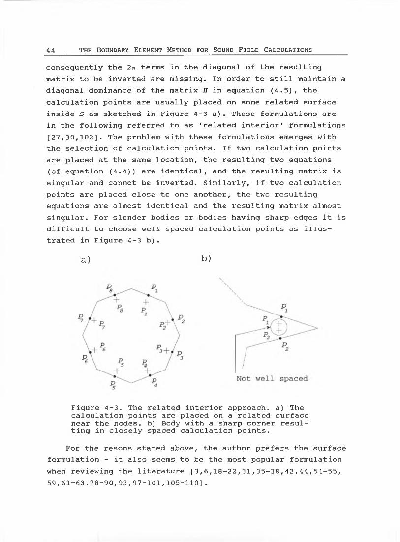
consequently the 2n terms in the diagonal of the resulting matrix to be inverted are missing. In order to still maintain a diagonal dominance of the matrix H in equation (4.5), the calculation points are usually placed on some related surface inside S as sketched in Figure 4-3 a). These formulations are in the following referred to as 'related interior' formulations [27,30,102]. The problem with these formulations emerges with the selection of calculation points. If two calculation points are placed at the same location, the resulting two equations (of equation (4.4)) are identical, and the resulting matrix is singular and cannot be inverted. Similarly, if two calculation points are placed close to one another, the two resulting equations are almost identical and the resulting matrix almost singular. For slender bodies or bodies having sharp edges it is difficult to choose well spaced calculation points as illus­trated in Figure 4-3 b).

a) b)

Figure 4-3. The related interior approach, a) The calculation points are placed on a related surface near the nodes, b) Body with a sharp corner resul­ting in closely spaced calculation points.

For the resons stated above, the author prefers the surface formulation - it also seems to be the most popular formulation when reviewing the literature [3,6,18-22,31,35-38,42,44,54-55, 59,61-63,78-90,93,97-101,105-110].

Bo u n d a r y El e m e n t M eth od - N u m e r i c a l Im p l e m e n t a t i o n 45

4.3 NUMERICAL INTEGRATION AND THE CONCEPT OF ORDERAs it has been demonstrated in section 4.1, the numerical

solution of Helmholtz integral equation may be divided into two major tasks: Numerical integration over the surface of the body in order to obtain the elements in the H and G matrices, and solution of the resulting system of linear equations. Hence numerical integration is an important part of the total numeri­cal solution, and is in fact often the most time consuming part of the total solution. Furthermore, some of the concepts of numerical integration may be used to explain the reasons for using more advanced functions to represent the variation of the pressure and the normal velocity than the constant value assumed in section 4.1.

4.3.1 THE LEFT RIEMAN SUMConsider the numerical evaluation of the integral

lba f w a x . (4.9)

where f(x) is a known function. Normally, a solution is desired which is suffiently accurate and obtained with as few evalu­ations of f(x) as possible, since the computational time comsumption almost always lies in the evaluation of f(x). For a simple numerical evaluation of equation (4.9) the interval [a,b] is divided into n small, equally sized elements of length h=(a-b)/n, as shown in Figure 4-4 a). The left Riemann sum is defined as the sum of the areas of the rectangular boxes with the height equal to the functions value in the start of each small interval and the width h=(b-a)/n:

n-1R„ = h 2 f (a+sh) . (4.10)

s=0

In order to investigate the convergence of the equation(4.10) it is assumed that feC1, where C1 is the set of func­tions for which the first derivative exists and is continuous.Consider the first element [a,a+h]; Taylor's formula for f states:

46 T he Bo u n d a r y E l em e n t M e t h o d f o r So u n d F ield Ca l c u l a t i o n s

a) b)

Figure 4-4. Numerical integration as a sum of areas, a) The left Rieman sum; b) The trapeziodal rule

f(x) = f(a) + (x-a) f'it) ; a<£<a+h , (4.11)

where f1 denotes df/dx, and £ is an unknown point in the interval. Integrating equation (4.11) over the interval [a,a+h] then yields

J a h t{x) dx = J a h f(a) +(a-h)f/(£) dx(4.12)

= hf (a) + iL. f ' ( 0 .

Adding n terms of this kind yields the integral over the entire interval [a,b]:

n ~1f f (x)dx = h f (a+sh) +h f1 ( rt) . (4.13)Ja s=o 2

Hence equation (4.10) calculates the desired integral with a certain error given by the difference between equations (4.13) and (4.10). This error is termed the truncation error since it is made by truncating the Taylor series for f(x) after a numberof terms, which in this case is one. If f1(x) is sufficiently smooth, the truncation error tends to zero asymptotically like h or 1/n when n tends to infinity. The left Rieman sum is said to be an integration formula of order one (g=l), since a reduc-

b o u n d a r y E lem e n t M eth od - N u m e r i c a l Im p l e m e n t a t i o n 47

tion of the element length from h to h/2 halves the truncation error, i.e. err2n/errn=( l/2)q=l/2 for g=l.

4.3.2 THE TRAPEZIODAL RULEIn order to obtain faster convergence one could consider

the trapezoidal rule. In this case the function is approximated by a straight line between the values of the endpoints of each element as shown in Figure 4-4 b). Hence, the integral is approximated by a sum of areas of trapezoids, which gives the formula its name. For the trapezoidal rule the following relation can be obtained [14]:

Ih f (x) dx = h a - h ^ f " U n )-i (f (a) +f (b)) + £ f (a+sh)z s-l

(4.14)where it is assumed that feC2. The order q of the trapeziodal rule is two since if h is reduced to h/2 the truncation error reduced to (1/2)2 = 1/4.

Roughly, these numerical integration formulas can be said to be constructed by dividing the interval to be integrated into elements. The function is then interpolated over each element by a polynomial, which may be integrated analytically. For the left Rieman sum the interpolation function is a con­stant, and for the trapeziodal rule the interpolation function is a first order polynomial. Generally, if f e Cw, an interpo­lation function of order 1 takes into account 1 + 1 terms of the function's Taylor series, resulting in an integration formula of order 1 + 1. However, using second order interpolation func­tions, which gives Simpson's rule, one should expect a formula of order three, but due to a fortunate cancellation of third order terms, Simpsons formula is of order four.

48 T he Bo u n d a r y El e m e n t M eth od f or So un d F ield C a l c u l a t i o n s

4 .3.3 a simple exampleConsider the numerical evaluation of the integral

Clearly, yfx is Cm in the interval [1,4]. Table 1 shows the error made by the left Rieman sum, the trapeziod rule and Simpsons rule for different element sizes. The results are shown in 15 digits precision - the machine precision is about 10“19. For each row in table 1 the number of elements n are doubled, and hence the order of the method may be estimated by taking the ratio of the error of two succeeding rowserr2n/errn, this ratio equals (1/2) , where qe is the estimate of the order of the numerical integration formula. It is evident that the formulas stabilize on a constant value of the order, which agrees very well with the theoretical value - for the first coarse divisions the assumption of smoothness of the first derivative, which is not taken into account by the formula, is not met, and hence the estimated order differs from the theoretical.

i Rieman sum estimated order for Riemam sum

Trapeziodal rule estimated order for Trapezio­dal rule

Simpsons rule estimated order for Simpsons rule

1 1,666666666666667 0,166666666666667 0,0043890064982872 0,794958421540382 1,06801 0,044958421540382 1,89030 0,000445958360282 3,298914 0,386574074155307 1,04013 0,011574074155307 1,95769 0,000035292872308 3,659468 0,190419988193058 1,02156 0,002919988193058 1,98686 0,000002407760470 3,8736116 0,094481802868617 1,01108 0,000731802868617 1,99644 0,000000154465166 3,9623432 0,047058066566029 1,00559 0,000183066566029 1,99909 0,000000009721116 3,9900264 0,023483273932344 1,00281 0,000045773932344 1,99977 0,000000000608639 3,99746128 0,011730193939565 1,00141 0,000011443939565 1,99994 0,000000000038057 3,99936256 0,005862236013434 1,00070 0,000002861013434 1,99999 0,000000000002379 3,99984512 0,002930402755143 1,00035 0,000000715255143 2,00000 0,000000000000149 3,99997

1024 0,001465022563897 1,00018 0,000000178813897 2,00000 0,000000000000009 3,999452048 0,000732466578481 1,00009 0,000000044703481 2,00000 0,000000000000001 3,997524096 0,000366222113371 1,00004 0,000000011175871 2,00000 0,0000000000000008192 0,000183108262718 1,00002 0,000000002793968 2,00000 0,000000000000000

Table 1. Error made by various numerical integration formulas. The estimated order is also shown.

VO

Boundary Element

Method

- Numerical

Implementation

50 T he Bo u n d a r y E l em e n t M e t h o d f o r Soun d F ield Ca l c u l a t i o n s

Another way of showing the convergence of numerical inte­gration formulas is to plot the error as a function of the number of function evaluations in double logaritmic scale, see Figure 4-5. The order qe may then be estimated as the slope of the curve.

number of function evaluations

Figure 4-5. The error vs. number of function evaluations of various numerical integration formulas.

It is evident from Figure 4-5 that Simpsons rule performs better than both the trapeziodal rule and the left Rieman sum in evaluating the integral of equation (4.15). Due to the high order of Simpsons rule compared to the order of the trapeziodal rule or the left Rieman sum, the superiority of Simpsons rule becomes increasingly pronounced as the demand of accuracy is raised.

The numerical integration formulas investigated so far are all based on equally spaced abscissas. Generally, when using a polynomial of order 1 requiring about 1 evaluations of the function per element, a numerical integration formula of order 1+1 is obtained. Now, if we allow for arbitrarily spaced

Bo u n d a r y E lem e n t M ethod - n u m e r i c a l i m p l e m e n t a t i o n 51

abscissas for evaluation of the function as well, twice the degree of freedom is obtained. In this case it may be shown [96] that a formula using 1 function evaluations per element has the order 21. These formulas are called Gaussian quadrature formulas, and the most common of these formulas is the Gauss- Legendre quadrature:

Tables over the abscissas x± and weights w± can be found in e.g. references [8,96]. The abscissas are also termed the Gauss points. The error made when using a 10 point Gauss-Legrendre quadrature (in the following often shortened to Gaussian quadrature) for the integral in equation (4.15) is also plotted in Figure 4-5, and it is evident that this formula performs far better than the other formulas considered. For a 10 point Gauss-Legendre formula the order is 20 (!), but the formula seldom behaves that well, since the assumption of a smooth 21st derivative is seldom met. Furthermore, v/hen increasing the number of elements the truncation error made by this formula quickly becomes less than the machine precision and hence the performance is limited by round-off errors. In Figure 4-5 round-off errors is seen to be dominating for more than 40 function evaluations.

Another advantage associated with Gauss-Legendre quadrature is that the function to be integrated is not evaluated at the endpoints of the interval. The Gauss-Legendre quadrature formula is therefore called an open formula, whereas formulas that do require the function to be evaluated at the endpoints, such as the trapeziodal rule and Simpsons rule, are termed closed formulas. If the Gauss-Legendra formula with an even number of points (like the 10 point formula) is chosen, the function is neither evaluated at the midpoint of the interval. These properties become important v/hen the function to be evaluated is singular or undefined at the midpoint or endpoints of the interval.

(4.16)

52 T he Bo u n d a r y El e m e n t M eth od for s o u n d F ield Ca l c u l a t i o n s

4 .3.4 integrals of singular functions The integral

r1 yfcdx = 1 (4.17)JO 3

is singular, since d (\[x ) /dx=l/ {2\fx) goes towards infinity as xgoes towards zero. The error made by the various formulations vs. the number of function evaluations is shown in Figure 4-6.

number of function evaluations

Figure 4-6. The error vs. number of function evaluations when the function to be integrated contains a singularity.

In this case we find that the high order formulas do not converge as quickly as they did for the non-singular integral in equation (4.15). Although the error made for a given number of function evaluations is still smaller when using Gaussian quadrature than when using e.g. Simpsons rule, the slope of the curves for the trapeziodal rule, Simpsons rule and Gaussian quadrature is the same. Hence the main benefit of using a high order formula has vanished. The slope of the curves for the trapeziodal rule, Simpsons rule and Gaussian quadrature is

Bo u n d a r y E lem ent m e t h o d - N u m e r i c a l Im p l e m e n t a t i o n 53

3/2=l/2+l, which corresponds to the fact that the function has a singularity of order 1/2 in its first derivative. Thus it is seen that for these numerical integration formulas the conver­gence is limited by singularities of the function, whereas the limiting factor of the left Rieman sum still is the order of the integration formula since the order of this formula is less than 3/2.

It can be seen from Figure 4-6 that the Gauss-Legendre quadrature formula still performs best in the singular case although the order benefit is destroyed. It can be shown [96] that the Gauss-Legendre quadrature formula will perform at least as good as any other formula with the same number of function evaluations, unless the formula is specially designed to deal with the singularity in question.

4.3.5 CONCLUDING REMARKSNumerical integration of a known function is carried out by

dividing the integration interval into small elements. For each element the function is evaluated at a finite number of points, and in between these points the function is approximated by an interpolation function. Thus the integral is approximated by a sum of products of the function evaluated at certain points and some weights. The weights are determined by the element length and the interpolation function.

If one uses an advanced interpolation function, a high order formula is obtained. However, a high order formula corresponds to high accuracy only if the function to be inte­grated is sufficiently smooth.

54 T he Bo u n d a r y E l e m e n t M ethod for S ound F ield C a l c u l a t i o n s

4.4 IMPLEMENTATION OF THE AXISYMMETRIC INTEGRAL EQUATIONFORMULATIONAs was shown in chapter 3, the surface integral of the

Helmholtz integral equation may be reduced to a line integral over the generator of the body and an integral over the angle of revolution. Since the angular dependance of the pressure and normal velocity could be described by their values on the generator due to the expansion in a cosine series, only the integral over the generator has to be discretized. The approach using constant elements would be to divide the generator into linear elements and place the nodes in the centre of each element, as sketched in Figure 4-2. However, the discussion in section 4.3 suggests a more advenced numerical treatment of the integral in equation (3.36). In this section three numerical implementations of equation (3.36) will be presented - one using linear interpolation functions, one using quadratic interpolation functions, and one using a combination of linear and quadratic elements. It should be noted that two fundamen­tally different types of interpolation are made in the numeri­cal treatment of equation (3.36). The first type concerns the interpolation of the pressure and the normal velocity between the nodes. The second type of interpolation concerns the geometry of the body; in practice the body is not described as a mathematical formula (or curve) but as a set of geometrical points: the nodes. In between these geometrical nodes the geometry is approximated with interpolation functions analogous to the interpolation of the pressure and the normal velocity. For this reason the interpolation functions are often referred to as shape functions.

4.4.1 LINEAR ELEMENTSConsider a linear variation of the pressure and the normal

velocity over each line element of the generator of the body. A body having N elements then has M=N+1 nodes, as sketched in Figure 4-7 a). Thus linear shape functions are used to repre­sent both the geometry and the acoustic variables. Dividing the generator of the body into linear elements allows equation

Bo u n d a r y E l e m e n t M ethod - N u m e r i c a l Im p l e m e n t a t i o n 55

(3.36) to be approximated byN

c(P)pra(P) * £ J-l

L P m ( Q ) F B ( P , Q , m ) dLg i Lj

N

+ ikz0 Y, [r vm {Q)FA{P,Q,m) dLQ j=1 )Lj

(4.18)

+ 4Jrpj;(P).

The procedure is then to put pm and vm outside the integration with respect to L.

■ >P

(Pj+1* zj+1)

Figure 4-7. Discretization of the generator of an axisymmetric body into linear elements. The z-axis is the axis of revol­ution. a) Total geometry with element number j indicated, b) Definition of local geometry for element number j.

Consider the first integral on the right-hand side of equation (4.18), where i is associated with the collocation point P:

56 T he Bo u n d a r y E l e m e n t M eth od for So un d F ield Ca l c u l a t i o n s

fr Pm (Q)FB(PilQ,m) dLj

= f pm (Q)FB(PifQ fm) dLj .(4.19)

Introducing the linear shape functions

= - *2 = -• €6[-l»l] (4.20)

allows the local geometry to be defined as

p(£) = Pj4>\{i) + Pj+3>2(£) z(0 = + z-/+i*2U)

(4.21)

The jacobian of this transformation J(£) =\/(dp/d£) 2 + (3z/302is J(£)=Lj/2, i.e. the ratio between the lengths of the inte­gration intervals in the two domains. The pressure is interpo­lated using the same shape function, as seen Figure 4-7 b), so that

PU) = Pj<*> iU) + Pj+i*2(0, (4.22)

where the expansion index m is omitted for convenience. It is now possible to express the integral of equation (4.19) in terms of the local coordinate £:

f p(Q)FB(PilQ,m) dL,

= J_\ {Pj(Z)*iU)+Pj+1(Z)4>2(t))FB(P±'Z'm)^-dZ (4‘23)

Pj^ij + Pj+l^ij •

where

h lj = J.\ d?

lj = ’t>2( ^ F B(Pi^,m)^2 d? ■(4.24)

It should be noted that the functions to be evaluated in the

BOUNDARY ELEMENT METHOD - NUMERICAL IMPLEMENTATION 57

1 2 • • integrals h±j and are almost identical. They consist of a

shape function (either or <f>2) which is fast to evaluate times a function FB. FB is quite computationally intensive since this function contains an integral over the angle of revolution as well as the evaluation of elliptic integrals.

1 2Hence, it is advantageous to evaluate the integrals and h±jsimultaneously reusing the evaluations of FB. It may also be noted that when using the open Gaussian quadrature formula, the function FB is not required at the nodal points (the endpointsof the integration interval), where it may be singular due tothe singularity in the Green's function.

The integrals containing vm are handled analogously. Con­sidering element number j, the integral in the second term of equation (4.18) can be transformed to

f v(Q)FA(Pi,Q,m) dLi

= J_\ (4.25)

= vj glj * vj+i9ij .

where the expansion index m is omitted, and

df(4.26)

For the i'th calculation point equation (4.18) is now approximated by (still with the index m omitted)

CiPi = Plhj2 +p2(ft|2+h|2) +~+pJ-(h?j_1+h}J) +-+pMhjN)

ikz0[v1gjI*v2(gj1 +g}2) +-+vj (gfj-^glj) *-*v„gfN)(4 •27)

+ 4*pf ,

since the pressure pj and the normal velocity Vj at node j con­tributes to the j-l'st element and the j'th element. Using M

58 T he Bo u n d a r y E l e m e n t M eth od f o r So un d F ield Ca l c u l a t i o n s

calculation points placed at the M nodes allows a matrix equation to be set up:

CPm = Hm pm * Gm v„ + 4np* , (4.28)

where m is the expansion index of equation (4.18).The matrices in equation (4.28) are defined as follows:

c =

C, 0

0 ... 0 Ci 0 - 0

0 cM

(4.29)

and

^ 1 1 h ll+h12 h lN-l+hlNL 2

h lN

Hm = *il *” h ±N-l+h±Nh 2iN

( 4r

hMl+hM2 hMN-l+hMN * MM

’ s r i i

2 1 911 912

2 ,„1 9 i n-1+9 in 9 in

ii

U6

2 1 9±l+9i2

2 1 ■■■ 9iN-l+9iN 9±m

( 4•

19Ml

2 1

9m l +9m 22 1

" • 9m n -i +9 mn 9m m

By introducing the boundary conditions, the matrix equation (4.28) is transformed into the familiar set of equations:

Amxm = Ym t (4.32)

where xm is the unknown vector and ym is the known vector. For the problem of scattering from a rigid surface Am equals C-Hm

b o u n d a r y El e m e n t M eth od - N u m e r i c a l Im p l e m e n t a t i o n 59

of equation (4.30) and ym equals p * , and for a radiation

problem where vm is known, equals C-Hm and ym equals Gm of equation (4.31) times vm: ym = Gmvm. In both these cases xm equals pm.

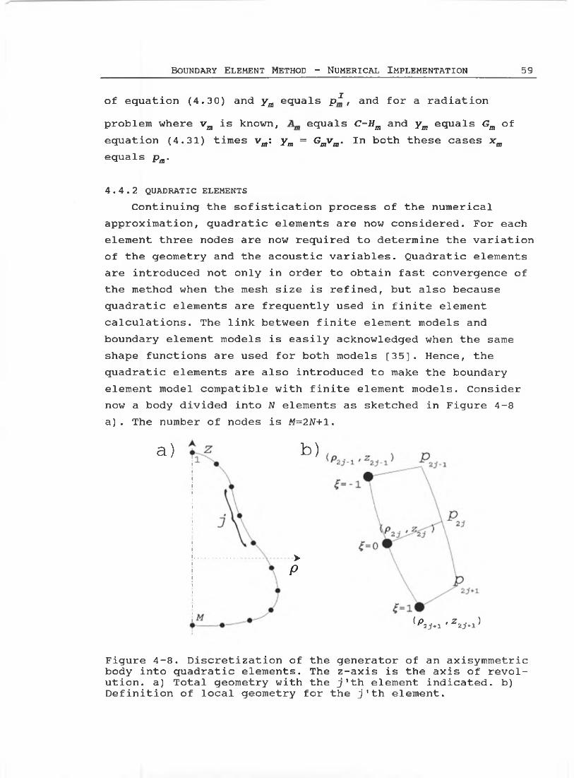
4.4.2 QUADRATIC ELEMENTSContinuing the sofistication process of the numerical

approximation, quadratic elements are now considered. For each element three nodes are now required to determine the variation of the geometry and the acoustic variables. Quadratic elements are introduced not only in order to obtain fast convergence of the method when the mesh size is refined, but also because quadratic elements are frequently used in finite element calculations. The link between finite element models and boundary element models is easily acknowledged when the same shape functions are used for both models [35]. Hence, the quadratic elements are also introduced to make the boundary element model compatible with finite element models. Consider now a body divided into N elements as sketched in Figure 4-8a). The number of nodes is M=2N+1.

a) b)

•>P

(P2>1 ' Z2j*l

Figure 4-8. Discretization of the generator of an axisymmetric body into quadratic elements. The z-axis is the axis of revol­ution. a) Total geometry with the j'th element indicated, b) Definition of local geometry for the j 1th element.

60 T h e Bo u n d a r y E lem e n t M eth od f o r Soun d F ield c a l c u l a t i o n s

Clearly, the quadratic shape functions represent a curved geometry better than the linear shape functions. Again, the integral over the generator is divided into a sum of integrals over each element as in equation (4.18), but for the same number of nodes the 'quadratic model1 has only half the elements of the 'linear model'. The integral over element number j with respect to collocation point i now states

f pm(Q)FB(Pi,Q,m) cLL- J LJ (4.33)=j pm {Q)FB{Pi,Q,rn) dLj .( 2J-1' z2j-l)

The shape functions for quadratic elements are [8,82]:

*1 = ^(g2~1) - *2 = !-«2 - *3 = {(V 1> ' • <4‘34>

Thus the local geometry, as seen in Figure 4-8 b) may now be described by

p(€) = />2 7-1^1 ( ) +P2 7 2 ( ) +^2 7+1^3 ( £ ) (4.35)Z(i) = Z2j-1<l>1(t)+Z2j<f>2(Z)+Z2j + 1<t>3(£) *

The jacobian of this transformation J (£.)=>! {d p/d$) 2 + (dz/d£)2 involves the derivatives of the shape functions:

-|t = ~2P2jt +P2j+l(^+^)(4.36)

=Z2J-l(?-|)-2z2j«+z2j+l(«+|) •

Note that for quadratic elements the unit normal vector n also varies with £. If the nodes are numbered clock-wise n may be found from the (p,z) coordinates by

n =(-£[£,£|). (4.37)

For counter clock-wise numbering the sign of the right side must be changed. For the linear elements described in the above paragraph the normal vector is constant within each element.

Bo u n d a r y E lem e n t M ethod - N u m e r i c a l Im p l e m e n t a t i o n 61

Using the same shape functions for the pressure:

P(£) = P2j-l^l (£ ) +P2j' 2 (£) +P2j'+1^3 (£) / (4.38)

where the expansion index m is omitted for convenience, allows equation (4.33) to be rewritten as

where

hh = J-i ■t‘l U ) F B(Pi,i,m)J(i)^ (4 . 40a, b, c)

hlj = <t‘3 U ) F B(Pi,Z ■

Once again a large amount of computational time may be saved by reusing the evaluation of FD when evaluating the integrals of equations (4.40a,b,c). Note that a Gaussian quadrature formula of even order should be used to evaluate the integrals of equations (4.40a,b,c) since then FB is not required for either <=-l,£=0 nor £=1, where FB may be undefined due to the singu­larity in Green's function.

The integrals containing vm are handled analogously, and placing M collocation points on the M nodes allows a matrix equation similar to equation (4.18) to be set up:

c Pn = HnPm + Gm vm * 4* Pm ■ (4-41)

where m is the expansion index of equation (4.18). The matrices of equation (4.41) are defined as follows (note that the middle node corresponding to £=0 is in contact with only one element):

62 T he Bo u n d a r y E le m e n t m e t h o d f o r s o u n d F ield Ca l c u l a t i o n s

c =

0 cM

(4.42)

and

^11 A?! h ll+h12 h212 •" h lN-l+hlN,2h lN IN

= I 'l l h il+hx2h212 *" h lN-l+tllN ,2

h±N h±N f(4.43)

I'm hMl+hM2u2 AM2 ^MN~1+ MN V,2

MN MN

*Ji 9ii3 1

9ll+9l2 9l2 9 i n -i +9 in2

9 IN

•9 IN

Gm = Sr]j 9il3 1

9il 9i2 9 2i2 •” 9 i n -i +9 in2

9 IN 9 IN •(4.44)

9mi 9m i3 1

9 Ml +9m22

9m 23 1

" • 9MM-1+9MM2

9m n3

9MN

The matrix equation (4.41) is transformed into the familiar set of equations by applying the boundary conditions.

4.4.3. SUPERPARAMETRIC ELEMENTSIf the same shape functions are used for discretizing both

the geometry and the acoustic variables the elements are termed 'isoparametric'. This is the case for the linear elements described in paragraph 4.4.1 and the quadratic elements described in paragraph 4.4.2. Isoparametric elements is by far the most well known element type in boundary element method formulations for acoustics. In fact, the use of non-iso- parametric formulation for acoustics has not been reported in the litterature as far as the author knows. However, as the isoparametric quadratic formulation was tested for radiation problems some annoying fluctuations of the solution was observed, which does not occur using isoparametric linear

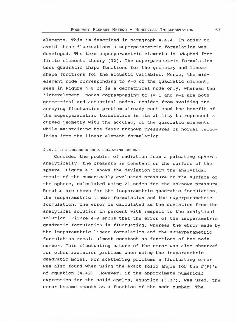
Bo u n d a r y E lem e n t M eth od - N u m e r i c a l Im p l e m e n t a t i o n 63

elements. This is described in paragraph 4.4.4. In order to avoid these fluctuations a superparametric formulation was developed. The term superparametric elements is adapted from finite elements theory [32]. The superparametric formulation uses quadratic shape functions for the geometry and linear shape functions for the acoustic variables. Hence, the mid­element node corresponding to £=0 of the quadratic element, seen in Figure 4-8 b) is a geometrical node only, whereas the 'interelement1 nodes corresponding to £=-1 and £=1 are both geometrical and acoustical nodes. Besides from avoiding the annoying fluctuation problem already mentioned the benefit of the superparametric formulation is its ability to represent a curved geometry with the accuracy of the quadratic elements while maintaining the fewer unknown pressures or normal veloc­ities from the linear element formulation.

4.4.4 THE PRESSURE ON A PULSATING SPHEREConsider the problem of radiation from a pulsating sphere.

Analytically, the pressure is constant on the surface of the sphere. Figure 4-9 shows the deviation from the analytical result of the numerically evaluated pressure on the surface of the sphere, calculated using 21 nodes for the unknown pressure. Results are shown for the isoparametric quadratic formulation, the isoparametric linear formulation and the superparametric formulation. The error is calculated as the deviation from the analytical solution in percent with respect to the analytical solution. Figure 4-9 shows that the error of the isoparametric quadratic formulation is fluctuating, whereas the error made by the isoparametric linear formulation and the superparametric formulation remain almost constant as functions of the node number. This fluctuating nature of the error was also observed for other radiation problems when using the isoparametric quadratic model. For scattering problems a fluctuating error was also found when using the exact solid angle for the C(P)' s of equation (4.42). However, if the approximate numerical expression for the solid angles, equation (3.37), was used, the error became smooth as a function of the node number. The

64 T he Bo u n d a r y E lem e n t M eth od for So un d F ield Ca l c u l a t i o n s

author has not yet found an expiation for this behaviour. Clearly, if calculating e.g. the radiated acoustic power, the resulting error would not be as large as the error observed for the pressure at each node, since in this case the error at each node would 'cancel out' to some extent. However, the error would still be unexpectedly large compared to the less sofisti- cated superparametric formulation.

Figure 4-9. Error made by the three formulations when calcu­lating the pressure on a pulsating sphere at ka=l .---□---,isoparametric quadratic formulation; ---+--- , isoparametriclinear formulation; ---*--- , superparametric formulation.

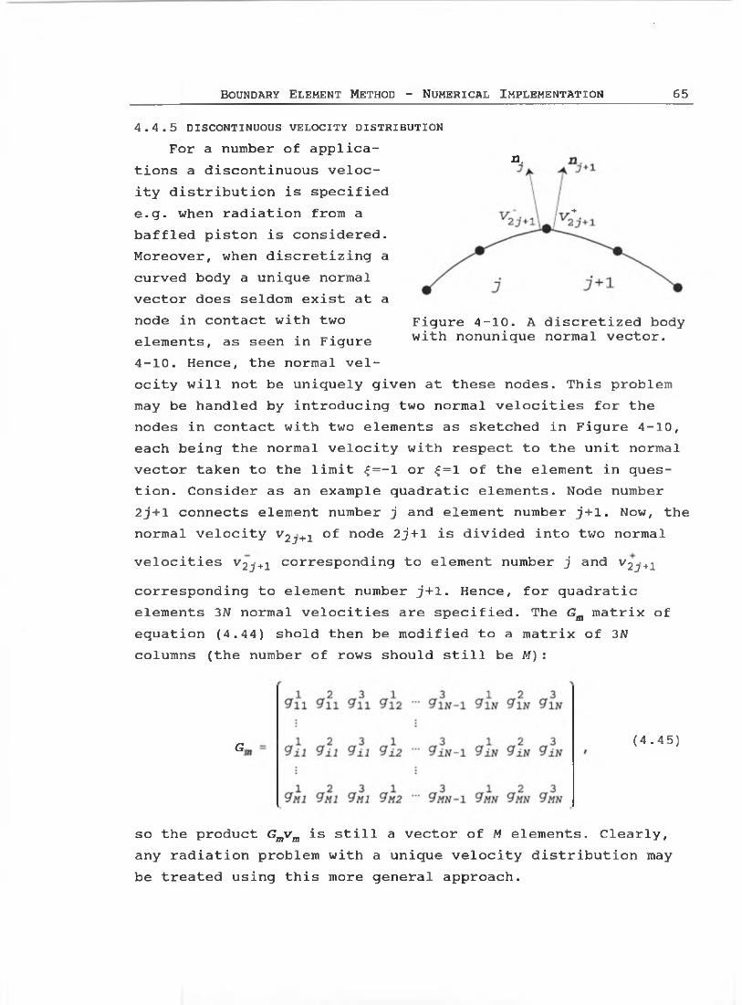
BOUNDARY ELEMENT METHOD - NUMERICAL IMPLEMENTATION 65

4.4.5 DISCONTINUOUS VELOCITY DISTRIBUTION For a number of applica­

tions a discontinuous veloc-n.

ity distribution is specified e.g. when radiation from a +baffled piston is considered. Moreover, when discretizing a curved body a unique normalvector does seldom exist at a node in contact with two Figure 4-10. A discretized body

with nonunique normal vector.elements, as seen in Figure4-10. Hence, the normal vel­ocity will not be uniquely given at these nodes. This problem may be handled by introducing two normal velocities for the nodes in contact with two elements as sketched in Figure 4-10, each being the normal velocity with respect to the unit normal vector taken to the limit £=-1 or £=1 of the element in ques­tion. Consider as an example quadratic elements. Node number 2j + l connects element number j and element number j+1. Now, the normal velocity v2j+1 of node 2j + l is divided into two normalvelocities v2j+1 corresponding to element number j and v2J+icorresponding to element number j+1. Hence, for quadratic elements 3N normal velocities are specified. The Gm matrix of equation (4.44) shold then be modified to a matrix of 3N columns (the number of rows should still be M):

G, (4.45)

so the product Gmvm is still a vector of M elements. Clearly, any radiation problem with a unique velocity distribution may be treated using this more general approach.

66 T h e Bo u n d a r y E le m e n t M eth od for So u n d F ield Ca l c u l a t i o n s

For linear elements an analogous approach may be used. In this case the Gm matrix consists of 2N columns and M rov/s.

4.5 TEST CASESTo verify the axisymmetric integral equation formulation

desbribed in chapter 3 and to demonstrate its advantages a number of test cases have been run using linear elements. Scattering as well as sound radiation has been tested.

4.5.1. APPLICATIONS TO SCATTERINGThe first test case is the scattering of a plane wave by a

rigid sphere of radius a. Since the sphere is axisymmetric v/ith respect to the z-axis, the plane wave is supposed to be travelling along the negative p-axis in order to involve all terms in the cosine expansion of equation (3.5).

Angle w (degrees)

Figure 4-11. Pressure on the surface of a sphere v/hen scatter­ing of a plane incoming wave for ka=1 is considered.-------- , analytical solution; boundary elementcalculation, 2 t e r m s / boundary element calculation, 3 terms; ■----, boundary element calculation, 4 terms.

Bo u n d a r y E l e m ent M e t h o d - N u m e r i c a l Im p l e m e n t a t i o n 67

Figure 4-11 shows the modulus of the complex pressure on the surface of the sphere as a function of the angle defined in the small inset in the figure for the case ka=l.

The generator is modelled by 11 nodes, and the pressure calculated by truncating the sum (3.38) at jn—1, m=2 and m=3, is shown compared to the analytical solution. It is apparent that 4 terms are sufficient to describe the sound field accurately at this frequency.

In order to observe the effect of an increased frequency the problem was also run for ka=5 and modelling the generator by 26 nodes. Figure 4-12 shows the calculated pressure obtained by truncating the sum (3.38) at m=6, m=1 and m=8.

Angle w (degrees)

Figure 4-12. Pressure on the surface of a sphere when scatter­ing of a plane incoming wave for ka=5 is considered_________ ,analytical solution; □, boundary element calculation, 6 terms; *, boundary element calculation, 7 terms; +, boundary element calculation, 8 terms.

68 T he Bo u n d a r y E lem e n t M eth od for So un d F ield Ca l c u l a t i o n s

At this frequency 8 terms must be calculated in order to obtain an accurate solution? adding more terms does not improve the accuracy significantly. In order to obtain a better accu­racy the discretization must be refined. It may also be notedthat at high frequencies the integral of revolution F* becomesstrongly oscillating, and hence the numerical integration of this integral must be refined.

The second test case concerns the scattering of a plane wave from two rigid spheres, where the axis of symmetry is parallel to the wavefront of the incoming wave. The two spheres both have radius a and the distance between their centres is d=5a. The problem was run for ka=l using a 16 node discretiza­tion for each sphere.

node

Figure 4-13. Pressure on the surface of the upper sphere when scattering of a plane incoming wave by 2 spheres for /ca=l andd=5a is considered--------- , boundary element calculation;....... , approximative analytical; , i sphere.

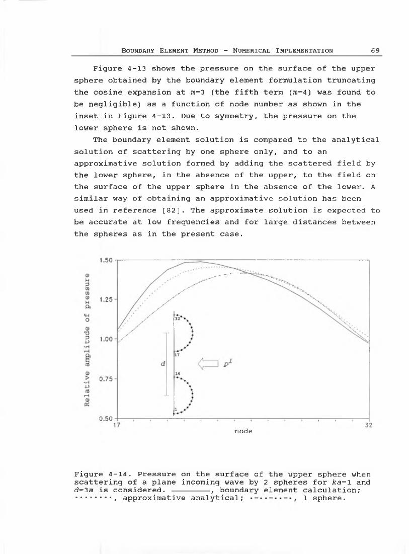
b o u n d a r y El e m e n t M e t h o d - N u m e r i c a l Im p l e m e n t a t i o n 69

Figure 4-13 shows the pressure on the surface of the upper sphere obtained by the boundary element formulation truncating the cosine expansion at m=3 (the fifth term (m=4) was found to be negligible) as a function of node number as shown in the inset in Figure 4-13. Due to symmetry, the pressure on the lower sphere is not shown.

The boundary element solution is compared to the analytical solution of scattering by one sphere only, and to an approximative solution formed by adding the scattered field by the lower sphere, in the absence of the upper, to the field onthe surface of the upper sphere in the absence of the lower. Asimilar way of obtaining an approximative solution has been used in reference [82]. The approximate solution is expected to be accurate at low frequencies and for large distances betweenthe spheres as in the present case.

node

Figure 4-14. Pressure on the surface of the upper sphere when scattering of a plane incoming wave by 2 spheres for ka=l andd=3a is considered. -------- , boundary element calculation;....... , approximative analytical; i sphere.

70 T he Bo u n d a r y El e m e n t M e th od for So un d F ield Ca l c u l a t i o n s

As the spheres become more closely spaced, the interacting scattering effect becomes more significant. Figure 4-14 shows the same results as seen in Figure 4-13, for the frequency ka=l but for a distance between the spheres of only c?=3a which means that the distance between the surfaces of the spheres is now only one radius.

In this case the boundary element solution formed by 4 terms of the cosine expansion (the fifth being negligible) differs more significantly from the approximate solution, although the approximate solution still provides a general image of the sound field.

4.5.2 APPLICATION TO RADIATIONAs an example of the application of this formulation to

radiation, the radiation from a vibrating sphere centered at (0,0,0) is considered.

w<D<DH<y>■c

<1JH3Ww<Daou<d

Angle w (degrees)

Figure 4-15. Pressure on the surface of a vibrating sphere for ka=1. -------- , mod(pressure) analytical; -------- , arg(pres­sure) analytical; *, mod(pressure) boundary element calcula­tion; #, arg(pressure) boundary element calculation.

In order to involve all terms in the cosine expansion, the normal velocity of the surface of the sphere is determined by

Bo u n d a r y E l e m ent M eth od - N u m e r i c a l Im p l e m e n t a t i o n 71

equating it with the velocity produced by a monopole q of unit strength (1 m3/s) placed at (pqfzq,dq)=(0.3,0.3,0). This method of generating the surface velocity of a sphere has been used in e.g. reference [78]. The boundary element formulation now produces a solution to this radiation problem, and this sol­ution may now be compared to the analytical solution of the monopole case. Figure 4-15 shows the pressure on the surface of the sphere as a function of the angle w to the p-axis for ka=l, using a 16 node discretization. Good agreement is found using four terms of the cosine expansion.

Finer discretization must be used to obtain a more accurate solution, since adding more terms of the cosine expansion does not improve the result at this frequency.

As a final testcase for radiation, the above problem was run for ka=2. Figure 4-16 shows that 4 terms of the cosine expansion still suffice to accurately predict the pressure on the surface of the sphere. However, finer discretization had to be used in order to calculate accurate values - in this case 30 nodes were used.

<3ft

(1)H303Wa>Hft•oe

(fi<DOu0)<D-o

OH2towowftcnuTJ

Angle w (degrees)

Figure 4-16. Pressure on the surface of a vibrating sphere for ka=2 . -------- , mod (pressure) analytical;---------, arg (pres­sure) analytical; *, mod(pressure) boundary element calcula­tion; #, arg(pressure) boundary element calculation.

72 T he Bo u n d a r y E l e m e n t M eth od f o r Soun d F ield Ca l c u l a t i o n s

4.5.3 CONCLUDING REMARKSThe axisymmetric integral equation formulation for non-

axisymmetric boundary conditions has been tested for radiation and scattering problems. For the problems considered only relatively few terms of the cosine expansion were required in order to obtain an accurate solution. Hence, the axisymmetric formulation requires much less calculation time and much less storage than a full three-dimensional numerical solution of the same problem - a comparison between the axisymmetric formula­tion and a three-dimensional formulation is given in paragraph 4.7.10. Further problems solved with the axisymmetric formula­tion using linear and quadratic elements are presented in chapters 7 and 8.

4.6 CONVERGENCEIn this section the convergence of the axisymmetric formu­

lations using isoparametric linear, isoparametric quadratic and superparametric elements will be discussed. Unfortunately, this situation is much less straightforward compared to the dis­cussion of convergence of numerical integration formulas in section 4.3, and in the literature only a few studys of conver­gence has been reported [59,99] In a boundary element formula­tion several approximations are made;a) The geometrical shape of the body is approximated using

shape functions.b) The acoustic variables are approximated using shape func­

tions.c) Numerical integrations of 'influence functions' are carried

out.d) The unknown acoustic variable are found numerically by

solving a set of linear equations.Suppose that the round-off errors made by solving the set of equations and the error made by the numerical integration are insignificant compared to the errors due to the first two approximations. For the 10 point guassian quadrature formula used here, this is indeed true. In fact, in order to optimize the formulation with respect to calculation time a more coarse

Bo u n d a r y E lem e n t M e t h o d - N u m e r i c a l Im p l e m e n t a t i o n 73

numerical integration formula should be used. In the test cases considered in the following, the frequency and body shape is chosen so that the resulting system of equations is well conditioned. Hence, round-off errors due to the numerical sol­ution of the set of equations are negligible.

Under these assumptions only the approximations related to the geometry and the acoustic variables are considered. If scattering from a rigid body is considered, only the pressure is discretized, since the normal velocity is zero, whereas radiation problems involve discretization of the normal veloc­ity as well. For this reason, the following discussion is divided into scattering and radiation problems.

The error made by discretizing the geometry corresponds to the difference between the solution of two problems. The first of these problems is the problem involving the 'real' body, and the second problem is the one where the body is subsituted with the discretized body as modelled by the shape functions. The behavior of this error is difficult to predict - it depends on the frequency, the shape of the body, and on the boundary conditions.

The error due to the discretization of the acoustic vari­ables should be comparable to the error made when interpolating a known function, which is to be integrated - i.e. similar to the error under study in section 4.3. In order for the problems considered here to resemble the situation described in section 4.3 as most as possible, the generator of the body is divided into elements of equal length. In practice elements of equal lenght would not be the optimum choice, and for several prob­lems such a division of the geometry would not even exist. For an optimal calculation (accuracy vs. calculation time) small elements should be used where the geometry or the acoustic variables vary quickly, whereas large elements should be used where the variation of these quantities is slow.

All in all, the curves presented in this section are expected to be straight lines in a double logarithmic coordinate system corresponding to an error proportional to hq, where q is the order of the formulation. However, becaurse of

74 T h e Bo u n d a r y E l e m e n t M eth od f o r So u n d F ield Ca l c u l a t i o n s

the unpredictable behaviour of the error due to the geometrical discretization, the curves might not be straight if this error is dominating.

4.6.1 SCATTERING BY A RIGID SPHEREIn Figure 4-17 scattering by a rigid sphere is considered.

In order to compare the three formulations, the error is shown as a function of the number M of acoustical nodes. For the isoparametric quadratic formulation the number of acoustical nodes equals 2N+1, where N is the number of elements. For both the isoparametric linear formulation and the superparametric formulation the number of nodes equals N+1. Since the time used for setting up the set of equations is proportional to M»N, the time used for setting up the set of equations is less for the isoparametric quadratic formulation than for the isoparametric linear formulation and the superparametric formulation. How­ever, the storage required for the set of equations and the time spend on solving the set of equations are the same in all three cases. For large M the total time used by all three formulations is dominated by the solution of the system of equations, since the time spend on matrix inversion grows as M3. For these reasons the author finds that the comparison between the three formulations is most fairly based on the number of unknowns M. The error is calculated as the length of the residual vector, which contains the difference between the analytical solution and the boundary element solution. Hence, when increasing the number of nodes, the number of terms in this error measure is also increased. Clearly, for each node the error is less than the error shown in Figure 4-17, but the error is generally not uniformly distributed over the nodes. This way of showing the error is a 'worst-case' method - the aforementioned fluctuating error of the isoparametric quadratic formulation for radiation is fully included, for instance. Figure 4-17 shows the error measure of the three formulations as functions of the number of acoustical nodes for ka=1, where a is the radius of the sphere. The incoming plane wave is of magnitude one (dimensionless for convenience). The figure shows

Bo u n d a r y El e m e n t M eth od - N u m e r i c a l Im p l e m e n t a t i o n 75

that the isoparametric formulation converges faster than the isoparametric linear formulation and also faster than the superparametric formulation.

Number of nodes

Figure 4-17. Error made by the three different boundary element formulations for scattering by a rigid sphere at ka-1. 0----, isoparametric quadratic formulation; +--,isoparametric linear formulation; ----*---- , superparametricformulation.

The slope of the curve for the isoparametric quadratic formulation is around -4, whereas the slope for both the iso­parametric linear formulation and the superparametric formula­tion is around -2. Since for scattering by a rigid sphere both the geometry and the pressure on the surface of the sphere have smooth high order derivatives, the convergence obtained here is expected to be close to the best possible.

When using isoparametric quadratic elements a rule of thumb is to choose the element size to be about half of the wave­length [107]. For the problem considered in Figure 4-17 this

76 T he Bo u n d a r y E le m ent M eth od f o r Soun d F ield Ca l c u l a t i o n s

discretization corresponds to 3 nodes, and the error found using the isoparametric quadratic formulation is 0.3. Note that the error is the squareroot of the sum of the squares of the error at each node. For the superparametric formulation the error using 3 nodes is 0.1, and for the isoparametric linear formulation the error using 3 nodes is 0.4. Hence, for this very coarse discretization the superparametric formulation performs best, whereas the isoparametric quadratic formulation performes best for finer discretizations.

4.6.2 SCATTERING BY A RIGID CIRCULAR CYLINDERIn order to investigate the

effect of discretizing the acoustic variables only, scattering by a rigid cylinder is now considered. In this case the geometry is completely described using 4 equally sized elements, as sketched in Figure 4-18.The length of the cylinder equals its diameter. Unfortunately, an analyti­cal solution of this problem does not exist. Hence, the 'analytical' sol­ution was produced as the boundary element solution with a very fine grid - the grid was refined until the difference between two calculations was negligible compared to the accu­racy obtained by the coarse division of the generator of the cylinder, used here to examine the convergence properties. Thus the 'analytical' solution is a boundary element solution using 160 isoparametric quadratic elements (321 nodes). Figure 4-19 shows the error made by the three formulations for the case of scattering by the rigid cylinder at ka=1. The incoming plane wave is again of magnitude one (dimensionless for convenience). Still, it appears that the isopametric quadratic formulation performes best. The curves for the isoparametric linear formulation and for the super-

Figure 4-18. The gene­rator of a cylinder divided into 4 ele­ments .

Bo u n d a r y E lem e n t M eth od - N u m e r i c a l Im p l e m e n t a t i o n 77

parametric formulation coincide. This is not unexpected, since the superparametric formulation may be regarded as a linear formulation with improved geometric interpolation. In the case of a circular cylinder, the generator consists of straight lines, which means that the improvement with respect to geometry has vanished.

Number of nodes

Figure 4-19. Error made by the three different boundary element formulations for scattering by a rigid cylinder at ka=1. □----, isoparametric quadratic formulation; n ,isoparametric linear formulation; ----*----, superparametricformulation.

The most noticeable feature of Figure 4-19 is the fact that all the curves have the same slope, which is around -0.7. This is probably due to the sharp edge of the cylinder, which theoretically causes the particle velocity to be infinite near the edge. In practice the particle velocity would be finite due to the viscosity of the fluid, of course. The asymptotic behaviour of the pressure near an edge may be found by the

78 T he Bo u n d a r y E l e m e n t M eth od for Soun d F ield Ca l c u l a t i o n s

following loose study. Consider the sound field near the edge of the cylinder. For the diffraction problem, the term of interest is kr, where r is the distance from the edge. Now, for any finite frequency kr tends to zero when r tends to zero, but since the diffraction problem is only governed by kr it is mathematically legitimate to keep r constant and let k tend to zero instead, and still draw the same conclusions from the approximative study. Hence, in the limit of small r Laplace's equation may be used. For Laplace's equation, traditionally used in the limit of small k, it is well known [58, p.69] that an edge of angle 3*/2 produces a r-1/3 behavior of the flow velocity at the edge - the general rule is that an angle a produces a r*/01-1 behavior of the flow velocity. Hence, the particle velocity tends to infinite as r tends to zero. The well known r-1/2 behaveior of the particle velocity near the edge of a thin screen [69, p.505,108-109] may also be explained in this way.

From the analysis of numerical integration it became clear that a singularity in a function would destroy the main benefit of a high order method, and this is what the author assumes is the reason for the behaveior of the curves in Figure 4-19. The case of scattering by a rigid cylinder is reconsidered in paragraph 9.1.2.

In fact, also the sphere has edges when modelled as dis­cussed in paragraph 4.4.5. However, since the order of the singularity depends of the opening angle, the singularities are so weak in this case that the benefit of a high order formula­tion is not destroyed. The problem of singularity may also be seen immediately from equation (3.1), where dG(R)/dn occurs - clearly the normal vector n is not defined at the edge of the cylinder. In fact the assumptions for setting up Helmholtz integral equation has been violated by the introduction of these discontinuities - the reason why the theory still works is that it is only violated in a region of vanishing area.

As an example, consider the most coarse mesh used in the calculations presented in Figure 4-19. This mesh consists of 9 acoustical nodes, which for the isoparametric quadratic for­

Bo u n d a r y E le m e n t M eth od - N u m e r i c a l Im p l e m e n t a t i o n 79

mulation corresponds to about 3 elements per wavelength at ka=l. The error made by the isoparametric quadratic formulation for this mesh is about 0.05. In order to obtain the same precision with the isoparametric linear model or the superpara­metric model about 25 nodes must be used.

4.6.3 RADIATION FROM A PULSATING SPHEREWhen radiation from a pulsating sphere is considered, both

the pressure and, of course, the normal velocity are constant on the surface of the sphere. Hence this test case should isolate the approximation made with respect to the geometry. Figure 4-20 shows the error made by the three formulations for ka=l. The magnitude of the pressure on the surface of the sphere is in this case about 33 Pa, and the errors shown should, of course, be compared to this number. The fluctuating error of the isoparametric quadratic formulation is again fully included, which means that if e.g. the radiated acoustic power was calculated the error would be smaller.

Figure 4-20. Error made by the three different boundary element formulations for radiation from a pulsating sphere at ka—1. □----, isoparametric quadratic formulation; 1-- ,isoparametric linear formulation; ----*---- , superparametricformulation.

80 T he Bo u n d a r y E l e m e n t M eth od f o r So un d F ield Ca l c u l a t i o n s

For the isoparametric quadratic and the superparametric formulations the error is significantly reduced when refining the mesh from 3 to 5 acoustical nodes. Further refinement of the mesh does not improve the accuracy very much - the slope of the curves for a large number of nodes is around -0.5 for the isoparametric quadratic formulation and -0.75 for the super­parametric formulation. For the isoparametric linear formula­tion the curve has a slight arch. At three nodes the slope is around -2, but at 21 nodes the slope is around -1.5. Hence, the convergence declines as the number of nodes increases. For this reason it is not expected that the isoparametric linear formu­lation will perform better than the superparametric for a very large number of nodes, although extrapolation of the curves in figure 4-20 could indicate that this was the case. Clearly, the superparametric formulation performs far better than the isoparametric quadratic formulation and the isoparametric linear formulation. The error for 3 nodes, which corresponds to an element length equal to half a wavelength for the quadratic formulation, is about 0.5 Pa for the superparametric formula­tion. For the isoparametric quadratic formulation the error isabout 9.5 Pa, which corresponds to an average of 3 Pa or 10 %of the analytically calculated pressure at each node. For the isoparametric linear formulation the error is about 23 Pa.

4.6.4 RADIATION FROM A VIBRATING CYLINDERIn order to investigate the effect of discretizing the

acoustic variables only, radiation from a cylinder is now con­sidered. The normal velocity of the surface was determined by equating it with the velocity produced by a monopole q of strength one (1 m3/s) placed at the centre of the cylinder (pq,zq,0q) = (0,0,0). This method for generating a surface velocity for an arbitrary shape was also used in paragraph4.5.2 and is sometimes termed a One Point Source test [78]. Thesolution for the pressure on the surface of the cylinder calculated by the boundary element formulations, for this pre­scribed velocity distribution and with the monopole removed,

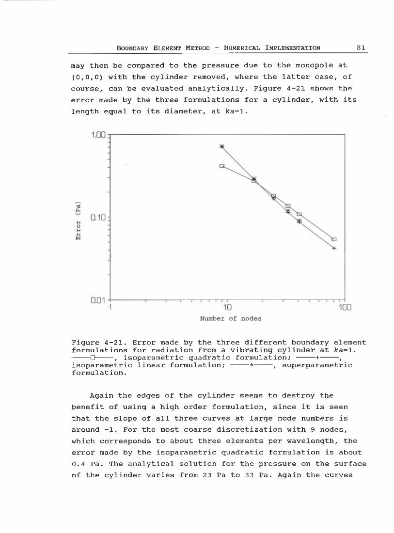
Bo u n d a r y E l em e n t M eth od - N u m e r i c a l Im p l e m e n t a t i o n 81

may then be compared to the pressure due to the monopole at (0,0,0) with the cylinder removed, where the latter case, of course, can be evaluated analytically. Figure 4-21 shows the error made by the three formulations for a cylinder, with its length equal to its diameter, at ka=l.

Figure 4-21. Error made by the three different boundary element formulations for radiation from a vibrating cylinder at ka=1. □----, isoparametric quadratic formulation; +--,isoparametric linear formulation; ----*---- , superparametricformulation.

Again the edges of the cylinder seems to destroy the benefit of using a high order formulation, since it is seen that the slope of all three curves at large node numbers is around -1. For the most coarse discretization with 9 nodes, which corresponds to about three elements per wavelength, the error made by the isoparametric quadratic formulation is about 0.4 Pa. The analytical solution for the pressure on the surface of the cylinder varies from 23 Pa to 33 Pa. Again the curves

82 T he Bo u n d a r y E le m e n t M e t h o d for Soun d F ield Ca l c u l a t i o n s

for the isoparametric linear formulation and the super­parametric formulation coincide due to the linear geometry.With 9 nodes the error made by these formulations is about 0.7 Pa. However, for more than 17 nodes the isoparametric linear formulation and the superparametric formulation performs slightly better than the isoparametric quadratic formulation.

4 .6.5 quarter-point techniqueIn paragraph 6.4.2 it was demonstrated that the benefit

with respect to convergence of using the high order quadratic shape functions was destroyed in the case of scattering of a plane wave by a rigid cylinder. It was justified that in this case the tangential flow velocity had a r-1/3 behavior near the edge of the cylinder. Hence, it was assumed that this singu­larity in the flow velocity destroyed the benefit of the high order formula. Recently Wu and Wan [108-109] has adopted the so-called quarter-point technique from the finite element method in order to efficiently handle the r-1/2 singularity of the flow velocity near a knife edge. It this case the pressure has a r1/2 behavior near the edge. Now suppose that the square- root function is to be approximated by the quadratic shape functions. The normal approach described in paragraph 4.4.2 ap­proximates the function by its values at the two endpoints and the midpoint of the interval, as shown in Figure 4-22 a). It can be seen in Figure 4-22 a) that when using the normal technique, the shape functions approximate the squareroot poorly. The quarter-point technique displaces the mid-element node to a position, where the distance to the singularity is one quarter of the lenght of the element. It can be seen in Figure 4-22 b) that when using this technique, the shape functions exactly model the squareroot function - in fact the two curves exactly coincides. It was shown in the paper by Wu and Wan [108] that the accuracy of the boundary element calcu­lations was dramatically improved when using this quarter-point technique.

Bo u n d a r y El e m e n t M e t h o d - N u m e r i c a l Im p l e m e n t a t i o n 83

Figure 4-22. Approximation of the squareroot function by quad­ratic shape functions, a) normal technique; b) quarter-point technique. -------- , squareroot function;-------- , approxima­tion by quadratic shape functions. The nodal points are indi­cated with bold dots on the x-axis.

Thus the idea of using a similar technique to model the r2/3 behavior of the pressure near the edge of the cylinder suggests itself. In order to do this, the r2/3 function was plotted and the mid-element node was displaced in order to obtain a good approximation of the r2/3 function near r=0. After a few attemp it was found that if the mid-element node was placed at a distance of 0.275 times the element length to the singularity,

84 T h e Bo u n d a r y E l e m e n t M eth od for So u n d F ield Ca l c u l a t i o n s

a good approximation of the r2/3 function was obtained as shown in Figure 4-23. Note, however, that the r2/3 function is not exactly represented by the shape functions, as was the case for the squareroot function.

x

Figure 4-23. Approximation of the r2 3 function by quadratic shape functions. -------- , r2/3 function; , approxima­tion by quadratic shape functions. The nodal points are indi­cated with bold dots on the x-axis.

The problem of scattering of a plane wave of unit magnitude by a rigid cylinder at ka=l was then re-calculated using this ge­neralized quarter-point technique. Figure 4-24 show the error of the original implementation using normal isoparametric quadratic elements and the error of the new implementation using isoparametric quadratic elements and the generalized quarter-point technique. The error is the length of the resid­ual vector, which contains the difference between the 'analy­tical' solution and the calculated solution at the two 'end- element' nodes. The reason for not including the mid-element

Bo u n d a r y El e m e n t M e t h o d - N u m e r i c a l Im p l e m e n t a t i o n 85

node was simply that the 'analytical' solution not readily produces a value at this node. The 'analytical' solution was the fine-meshed boundary element calculation also used in paragraph 4.6.2.

Number of nodes

Figure 4-24. Error made by the two boundary element formula­tions for scattering by a rigid cylinder at ka=l. n ,normal isoparametric quadratic formulation; ---+--- , general­ized quarter-point formulation.

It can be seen from Figure 4-24 that the formulation using the generalized quarter-point technique produces a much more accurate result than the normal formulation. Moreover, the generalized quarter-point technique seems to restore the high convergence rate of the isoparametric quadratic formulation.The author expects that any scattering problem with a singular­ity due to an edge, can be modelled accurately by an adequate placement of the mid-element node.

86 T he Bo u n d a r y E l e m e n t M eth od for So u n d F ield Ca l c u l a t i o n s

4.6.6 CONCLUDING REMARKSThe convergence of the three boundary element formulations

for the axisymmetric integral equation has been examined in four test cases. The test cases chosen should throw light on the effect of the approximations made regarding the geometry and the acoustic variables. The results presented here are mainly of theoretical interest, since an optimized formulation for practical use would be carried out with a more coarse integration over each element, so that the error due to this integration could not be neglected. Moreover, a pratical formulation would not use equally sized elements, as used for these test cases.

However, the test cases presented here may serve as an instrument to compare different boundary element formulations. It must be admitted that the calculations presented in this section merely outlines the topic of convergence, and some of the complications, which arise when this topic is examined. Much further theoretical work and further test cases should be made in order to investigate convergence of boundary element formulations adequately. It would also be interesting to evaluate the ability of different methods to overcome the non­uniqueness problem with respect to convergence, in a much more systematic manner than it has been done until now in the literature. The non-uniqueness problem is presented in chapter 5.

Finally, a generalized quarter-point technique was used to model the r2/3 behaviour of the pressure near the edge of a rigid cylinder when scattering an incoming plane wave. The generalized quarter-point technique improves the accuracy of the isoparametric formulation significantly and restores the high convergence rate of this formulation.

Bo u n d a r y E l e m e n t M e th od - N u m e r i c a l Im p l e m e n t a t i o n 87

4.7 IMPLEMENTATION OF THE THREE-DIMENSIONAL FORMULATIONA simple implementation of the Helmholtz integral equation

for three-dimensional problems using constant elements has been outlined in section 4.1. In this section the more advanced approaches, using elements corresponding to linear and quad­ratic shape functions, will be described [8,9,80,112]. Usually two types of elements are used: triangular and quadrilateral elements. The transformation of the three-dimensional Helmholtz integral equation into a set of linear equations will not be described as detailed as for the axisymmetric formulation, since the general ideas are the same. Thus, the elements of the difference formulations and the corresponding shape functions will merely be listed, and some comments on the transformation to a set of linear equations will be given. A three-dimensional boundary element formulation has been implemented using super­parametric elements, and test cases for this implementation will be presented.

4.7.1 LINEAR TRIANGULAR ELEMENTSIf the geometry is assumed to vary linearly between the

nodes, the global coordinates (x,y,z) are connected to the local coordinates of the elements as follows:

x = x 1£1+x 2<2+*3£3 'y = yi£i+y2<2+y3£3 * (4.46)Z = +z2^2+z3^3 *

Here ^3=l-^i~^2' anc* ibices for the global coordinatesrefer to the local node numbering defined in Figure 4-25. Clearly and |2 suffices in order to describe the planar tri­angular geometry - the reason for defining the dependant third coordinate is that the resulting equations then become neatly symmetric with respect to the ('s. Thus the shape functions for this case are simply

88 T h e Bo u n d a r y Ele m e n t M eth od f o r So un d F ield Ca l c u l a t i o n s

wi (£i'^2/£3) = £1 '^2 ^2/£3) = £2 • (4.47a,b,c)

tf3(*lr*2/*3> = ^3 /and the planar element described by the three sets of global coordinates (xl,y1,z1), {x2,y2,z2) > and (X3 >Y3 >Z3) is trans­formed into a planar triangular element in a (f j,t2'€3 ) system, as sketched in Figures 4-25 a) and 4-25 b). The (€1,£2,Z3) system is the well-known area-coordinate system frequently used in finite element methods, from where the term 'parent element1 for the element in Figure 4-25 b) is also adopted. The Jacobian of this transformation equals the ratio between the areas of the triangles, which is 2A, where A is the area of the element in Figure 4-25 a). Note that the parent element is shown in a way that underlines the symmetry with respect to the £'s and not in a right-angled coordinate system, and that the area of the parent element actually is 1/2.

a) b)

Figure 4-25. Transformation of a planar triangular element to its corresponding parent element, a) The planar element in the global coordinate system with local numbering of the nodes indicated, b) Corresponding parent element in local coordinate system with local node numbers indicated.

Bo u n d a r y El e m e n t M eth od - N u m e r i c a l Im p l e m e n t a t i o n 89

The pressure and the normal velocity may be expressed by the same shape functions:

3p(«l,«2»€3> = E wa(«l-f2'«3) Pc . (4.48)a=l

and3

= E Na(il'i2'(3) va • (4.49)a=l

In this case the element above is termed isoparametric linear triangular element.

4.7.2 QUADRATIC TRIANGULAR ELEMENTSIf a quadratic variation of the geometry is assumed 6 nodes

are required to describe the geometry. Figure 4-26 shows the transformation from the global coordinate system to the local coordinate system in this case.

a) b)

Figure 4-26. Transformation of a curved triangular element to its corresponding parent element, a) The curved element in the global coordinate system with local numbering of the nodes indicated, b) Corresponding parent element in local coordinate system with local node numbers indicated.

90 T he Bo u n d a r y E l e m e n t M eth od f or Sou n d F ield Ca l c u l a t i o n s

(4.50a-f)

The shape functions of this transformation are:

N2 (Sl'Z2>t3) = l2(2^2-D /^3 C^l/^2'^3) = £3(2^3”1) /

N4(*lt*2r*3) = 4^1^2/% ( ^ 1 ^ 2 ^ 3) = 4 2^ 3'N6(^lf^2'^3) = 4 £ l£ 3'

where €3=1-1i“£2• T^is leads to the following expression for the global coordinates for a point of the element, as a func­tion of the local coordinates (£j ,£2 **3):

6

* • ( « ! , e2*«3) = E wa ( e i , « 2 f?3) xQ ,a=l

6

y ( € l , ? 2 , « 3) = E nc « (€ i . « 2 - « 3 ) ya > (4 . 5 1 a , b , c )a-1

6

2 (€1 ,€2.«3> = E Nc ( « 1' «2-?3) za • a=l

The Jacobian of this transformation is

J ( « i , e 2,?3) = II O r / a ? 1) x ( a r / a ? 2) ||2 , (4 .52)

v/here r={x,y,z). Note that the Jacobian is the lenght of the normal vector:

n = , (4.53)8*1 8*2 K }

which is also needed to construct the normal derivative of Green's function.

The pressure and normal velocity are approximated using the same shape functions:

Bo u n d a r y E le m e n t M eth od - N u m e r i c a l Im p l e m e n t a t i o n 91

6

p(«l,«2»*3) = E Wa<fl'«2.*3) P a ' (4.54)a=l

and6

v (€1,«2/€3) = E »o(fl/f2»«3) - (4-55>

Thus, an isoparametric quadratic triangular element has been obtained.

4.7.3 LINEAR QUADRILATERAL ELEMENTSConsider the transformation of a plane quadrilateral

element to its parent element as sketched in Figure 4-27.

a) b)

( - 1 , - 1 )

(1,1)

fi

(1,-1)

Figure 4-27. Transformation of a planar quadrilateral element to its corresponding parent element, a) The planar element in the global coordinate system with local numbering of the nodes indicated, b) Corresponding parent element in local coordinate system with local node numbers indicated.

The shape functions of this transformation are:

92 T he Bo u n d a r y E le m e n t M ethod f or S oun d F ield Ca l c u l a t i o n s

W3(«l,«2) = 4(1+«l) (1+«2) »(4.56a-d)

(1+f, \ (1+?^) .

tf4Ui,*2> = (1 2) /

which leads to the following expression for the global coordinates for a point on the element in terms of the local coordinates:

4*Ul/C2) = Y, Ncc(tl't2)xa /a=l

4y«l»«2) = E *c.(«l- « 2)ya ■ (4.57a,b,c)a=l

4z (?l'«2> = E Wa<?l'?2) za • a=l

The Jacobian of this transformation equals A/A, where A is the area of the element in Figure 4-27 a). In order to obtain an isoparametric linear quadrilateral element, the pressure and normal velocity are approximated using the same shape func­tions :

4P(«l.«2> = E WQ(«l-«2) Pa ' <4‘58>a=l

and4

V(«l.f2) = E Na((lr(2) Va ■ <4-59>Q-l

Note that the unit normal vector is constant within each element.

4.7.4 QUADRATIC QUADRILATERAL ELEMENTSFinally, the quadratic quadrilateral element is considered.

In this case the geometry is assumed to vary in a quadratic

Bo u n d a r y E lem e n t M e th od - N u m e r i c a l Im p l e m e n t a t i o n 93

manner over each element. Now 8 nodes are needed for a descrip­tion of the geometry, as sketched in Figure 4-28.

a)

3 3'

b)

(-1,1) (0,1) 1,1)4 7 3

(-1,0)8 6 (1,0)

fi

1 5 2(-1 -l) (0.-i) (1,-l)

Figure 4-28. Transformation of a curved quadrilateral element to its corresponding parent element, a) The curved element in the global coordinate system with local numbering of the nodes indicated, b) Corresponding parent element in local coordinate system with local node numbers indicated.

The shape functions of this transformation are:

l-li) (i—£2) /

l+£i) (l-£2) U i-^2-1) >

l +€l ) ( 1 2) U l - ^ 2 " 1) '

l - £ i ) ( 1+C2) ( - l i +e2- l ) *

2 •

l'.

2 •

1

Ni U i,£2) = i■4 W i )

- 14 i+£i)

N3(tlfZ2) - 14 i+Ci)

N4(«i,|2) - 14 i-*i>

W5(^i^2) = 12 i-d)

^6(£ 1/£ 2) = 12 i-d)

tf7(*lf*2> = 12 i-d)

NQ(ii,s2) = 12 i-d)

(4.60a-h)

94 T he Bo u n d a r y E l e m e n t M eth od f or Sou n d F ield Ca l c u l a t i o n s

In this case the global coordinates of a point on the elementis related to the local coordinates as follows:

8

x («l-«2) = E Nc («1-«2) -Of = 1

8

y(€ 1»«2> = E Nc,(il’t2)ya ' (4 . 6 1a,b,c)a -1

8

z(«l,?2> = E Na((l'(2) zoc ■a=l

As was also the case for the quadratic triangular elements, theJacobian is the lenght of the normal vector n:

where r=(x,y,z). If now the pressure and normal velocity are expressed using the same shape functions:

8

P(«l.«2) = E Wc(«l'«2) Pa - <4-63>a=l

and8

v(«l.f2) = E Nc(t l.«2) - <4-64)a*l

an isoparametric quadratic quadrilateral element has been obtained.

4.7.5 s u p e r p a r a m e t r i c t r i a n g u l a r ele ment sIf the shape functions used to approximate the body are of

a higher order than the shape functions used to approximate the acoustics variables, the elements are termed superparametric [32]. Conversely, if the shape functions for the geometry are of a lower order than the shape functions of the acoustics variables, the elements are termed subparametric. In order to obtain superparametric elements, quadratic shape functions (equations (4.50a-f), (4.51a,b,c), (4.52), and (4.51)) are usedto discretize the geometry, whereas linear shape functions

Bo u n d a r y E le m e n t M eth od - N u m e r i c a l Im p l e m e n t a t i o n 95

(equations (4.48) and (4.49)) are used to discretize the acoustic variables.

As the quadratic shape functions was implemented for acoustic boundary element computations [80,81] it was stated that the main benefit of using these elements was the ability of the quadratic elements to represent curved surfaces, whereas the benefit of a better representation of the acoustic vari­ables was less significant. Furthermore, it was found in section 4.6, where convergence of the axisymmetric formulations was discussed, that singularities often caused the pressure to be only continuous. This destroys the main benefit of using high order shape functions, the benefit being faster conver­gence than obtained when using shape functions of lower order. Finally, since all programming of this project was carried out on a regular personal computer, it was important to use as few acoustical nodes as possible when calculating three-dimensional problems, in order to keep the sizes of the resulting matrices to within resonable limits. It was also found in section 4.6 that the error made by the axisymmetric superparametric formu­lation in three of the four test cases was smaller than, or of the same magnitude, as the error made by both the isoparametric linear formulation and the isoparametric quadratic formulation.

4.7.6 NUMBERING OF NODESFor the reasons outlined above a superparametric triangular

formulation was implemented for calculating three-dimensional problems.

When discretizing a three-dimensional problem, the relation between local and global node numbers are not as simple as when discretizing the generator of an axisymmetric body. Fortunate­ly, the numbering of nodes is not as critical for boundary element formulations as it is for the finite element method, where correct numbering is vital for the bandwidth of the resulting matrices and thus for the efficiency of the method. For boundary element calculations the resultating matrices are generally fully populated (all elements are non-zero), and the problem of reducing the bandwidth does nor occur.

96 T he Bo u n d a r y El e m e n t M eth od f o r So un d F ield Ca l c u l a t i o n s

10

Figure 4-29. Discretization of a sphere of radius one into 8 quadratic triangular elements, a) Perspective view, b) Upper hemisphere. The large number in the centre of each element is the element number, the normal sized numbers are the global node numbers, and the small numbers in brackets are the local node numbers.

Bo u n d a r y E le m e n t M e t h o d - N u m e r i c a l Im p l e m e n t a t i o n 97

As an example of how the data structures needed to describe the geometry are defined, and how the relation between local and global numbering of the nodes is obtained the discretiza­tion of a sphere is considered. Figure 4-29 a) shows the discretization of a sphere of radius one into 8 quadratic triangular elements, and Figure 4-29 b) shows the upper hemi­sphere. With the numbering indicated in Figure 4-29 the global (x,y,z)-coordinates of the geometrical nodes are listed in Table 2.

Globalnode

numberX y z

1 0 0 12 0,7071 0 0,70713 0 0,7071 0,70714 -0,7071 0 0,70715 0 -0,7071 0,70716 1 0 07 0,7071 0,7071 08 0 1 09 -0,7071 0,7071 010 -1 0 011 -0,7071 -0,7071 012 0 -1 013 0,7071 -0,7071 014 0,7071 0 -0,707115 0 0,7071 -0,707116 -0,7071 0 -0,707117 0 -0,7071 -0,707118 0 0 -1

Table 2. The global coordinates of the global geo­metrical nodes

A data structure is now needed which connects the local node number of each element to the global node number. An

98 T he Bo u n d a r y Ele m e n t M eth od for Soun d F ield Ca l c u l a t i o n s

example of this data structure for the sphere shown in Figure 4-29 is shown in Table 3. The table is read in the following way: For the 4'th local node of the 5'th element the global node number is 15, for instance.

elementnumber

local node 1

local node 2

local node 3

local node 4

local node 5

local node 6

1 1 6 8 2 7 32 1 8 10 3 9 43 1 10 12 4 11 54 1 12 6 5 13 25 18 8 6 15 7 146 18 10 8 16 9 157 18 12 10 17 11 168 18 6 12 14 13 17

Table 3. The global node numbers vs. the local node number and the element number.

For the superparametric formulation not all geometrical nodes are acoustical nodes as well - only the local geometrical nodes 1, 2 , and 3 of figure 4-29 b) are also acoustical nodes. For the discretized sphere in figure 4-29 there are 6 acousti­cal nodes with the global geometrical node numbers {1,6,8,10, 12,18}. Hence, for the superparametric formulation a further data structure must be defined, which establishes the relation­ship between the global geometrical node number and the global acoustical node number. This data structure, for the example of the sphere, is listed in Table 4.

In order to find the global (x,y,z) coordinates needed to calculate the source-receiver distance R of Green's function and its derivative, as a function of the integration variables £lf £2 and the dependent coordinate $3, the procedure is:Relate the local node number of the geometrical node to its global node number by a look-up in Table 3 and then find its global coordinates through Table 2.

Bo u n d a r y El e m e n t M eth od - N u m e r i c a l Im p l e m e n t a t i o n 99

Global acoustical node number

1 2 3 4 5 6

Global geometrical node number

1 6 8 10 12 18

Table 4. Relation between the global acoustical node number and the global geometrical node number.

The procedure for setting up the set of linear equations is as follows: Place the collocation point number i at the i'th acoustical node to form the i'th row of the 'influence' matrices H and G of equation (4.8). For each element a numeri­cal integration of the 'influence' functions is carried out and the result is referred to the corresponding local acoustical nodes (i.e. the local geometrical nodes 1, 2, and 3) through the acoustical shape functions of equations (4.48) and (4.49). The results of the integrations are referred to the global acoustical nodes through look-ups in Tables 3 and 4 and placed in the corresponding columns of the H and G matrices.

4.7.7 NUMERICAL INTEGRATION OF TRIANGULAR ELEMENTSFor the triangular elements in Figures 4-25 b) and 4-26 b)

special numerical integration formulas are given [8,112]. The formula used here is of order 6. The integration points and the corresponding weights is shown in Figure 4-30.

Note that the weights listed in Figure 4-30 adds up to one, and hence the result of the integration should be multiplied by the area of the triangle (1/2 for the triangular parent element).

100 T he Bo u n d a r y E lem e n t M eth od for Sou n d F ield Ca l c u l a t i o n s

Points Weightsa (1 /3 ,1/3 ,1/ 3 ) 0.2250000000

b (tr1,iS1 ,E 1) 0.1323941527

c ( flf i ) 0.1323941527

d <*1 , % , « ! > 0.1323941527

© < «2 ' * 2 ' * 2 > 0.1259391805

f ^ 2 ' a2'%) 0.1259391805

9 0.1259391805

with0.0597158717

0.4701420641

a ? ~ 0.7974269853

0.1012865073

Figure 4-30. Numerical integration formula for triangle. The Gauss points and the corresponding weights are also listed.

4.7.8 NUMERICAL INTEGRATION OF QUADRILATERAL ELEMENTSFor the quadrilateral parent elements of Figures 4-27 b)

and 4-28 b) numerical integration of a function f may be carried out by combining two one-dimensional Guassian quadrature formulas:

f. f , f(fl-<2) * E E t{Xi,Xj)WiW:i . (4.65)J-l J 1 J=1 i=l

Here the Gauss points (xi and Xj) and weights (w± and Wj) of the one-dimensional formula discussed in paragraph 4.3.3 are used.

4.7.9 SINGULAR INTEGRALSFor the integration over the elements in contact with the

collocation point, special care must be taken since the Green's function and its normal derivative contain singularities of order 1/R [75,81].

In reference [75] these integrals were handled by intro­

Bo u n d a r y El e m e n t M eth od - N u m e r i c a l Im p l e m e n t a t i o n 101

ducing a local polar coordinate system (r,9), such that the singularity was placed in r=0. In this way the singularity is neutral­ized due to the factor r in the Jacobian of the trans­formation. In references [8,29] specialized numerical integration formulas for tri­angles and quadrangles with an 1/R singularity is given.In the present work the idea due to Rizzo and Shippy [75] has been used, and the tech­nique will hence be outlined, for the case of a singularity at the corner of a triangle.

Consider the triangular parent element of Figures 4-25 b) and 4-26 b). If the singularity is placed at the local node number 1, the polar coordinate system (r,0) should be placed so that r=0 at the singularity as sketched in Figure 4-31. For this transformation

= l-rsin0 ,and = — rcosd + iirsintf (4.66)1 * 2 2

is found. The Jacobian of this transformation equals \fl/2 r.Note that mathematically this transformation is illegal due to the singularity of the function to be integrated, but this may be handled by excluding a small area of radius c around the singularity and then let c tend to zero. Thus the integral of the singular function f is transformed as follows:

JSj *<«,.«*> d?Jd?2 = 0 3 J01/rsin* t(r,e)^-rara6 ,(4.67)

Figure 4-31. Definition of lo­cal polar coordinate system for a triangular element with a singularity at the local node number 1.

and thereby the 1/R singularity of f is neutralized by the

102 T he Bo u n d a r y E le m e n t M e t h o d for So u n d F ield Ca l c u l a t i o n s

Jabobian of the trans­formation. The two-dimension­al integral on the right-hand side of equation (4.67) may be solved numerically by com­bining two one-dimensional Gaussian quadrature formulas as described in paragraph 4.7.8. Note that this method of numerically integrating the right side of equation (4.67) also has the advantage of close spacing of the Gauss points near the singularity as sketched in Figure 4-32.

Due to the symmetry of the £'s, the transformations in the cases where the singularity is placed at either local node 2 or 3 are easily found by suitable rotation of £2, £2, and in equations (4.66) and (4.67).

4.7.10 TEST CASESFor the superparametric triangular model a few test cases

has been calculated. The test cases all concern the very familiar case of scattering by a rigid sphere and they are compared to an analytical solution and to the superparametric axisymmetric formulation described in paragraph 4.4.3. The reason for not testing the three-dimensional formulation for a more complicated body shape is that the surface mesh is gener­ated 'by hand1 since at this moment no 'pre-processor' for generating the mesh is avaliable. Hence, at this stage, mesh generating is a quite time consuming task, and further verifi­cation of the three-dimensional formulation was not carried out.

Figure 4-33 a)-c) shows the pressure on the surface of a rigid sphere exposed to a plane wave of magnitude one (dimensionless for convenience) as functions of the angle

Figure 4-32. Gauss points for the element in Figure 4-31 using two one-dimensional 6 point Gaussian quadrature for­mulas .

Bo u n d a r y E l em e n t Me t h o d - N u m e r i c a l Im p l e m e n t a t i o n 103

Angle w (degrees)

Figure 4-33. Pressure on the surface of a sphere of radius a when scattering of a plane incoming wave is considered.a) ka=l, b) ka=2, c) ka=5. -------- , analytical solution;□, superparametric axisymmetric formulation; +, superparametric three-dimensional formulation.

104 T he Bo u n d a r y E l e m e n t M e t h o d for So un d F ield Ca l c u l a t i o n s

defined in the small inset in Figure 4-33 a). The test cases were run for ka=1 (Figure 4-33 a)), ka=2 (Figure 4-33 b) ) , and ka=5 (Figure 4-33 c) ) , where a is the radius of the sphere. In the figures three curves are shown: the analytical solution, the boundary element solution obtained by the superparametric axisymmetric formulation, and the boundary element solution obtained by the superparametric three-dimensional formulation. For the superparametric axisymmetric formulation 8 quadratic elements were used to model the generator of the sphere corre­sponding to 9 acoustical nodes on the generator. The super­parametric three-dimensional formulation used 168 quadratic triangular elements, which corresponds to 86 acoustical nodes. The acoustical nodes were placed in a manner, such that there were 9 acoustical nodes on the generator of the sphere for the three-dimensional formulation as well. Hence, the element size of the three-dimensional formulation is approximately equal to the element size of the axisymmetric formulation. The ratio of elements per wavelength is 16 for ka—1, 8 for ka=2, and 3 for ka=5. The figure shows that the results obtained by the axisym­metric formulation and the three-dimensional formulation are almost identical. Hence, it is concluded that the error made by the superparametric three-dimensional formulation for a given number of elements per wavelength is of the same size as the error made by the superparametric axisymmetric formulation for the same number of elements per wavelength. This indicates that the experience of accuracy vs. mesh fineness acquired in the case of the superparametric axisymmetric formulation can be transferred to the case of the superparametric three-dimension­al formulation.

For the highest frequency corresponding to ka=5 the maximum deviation between the analytical solution and the two boundary element calculations is about 0.15, or 15% of the magnitude of the incoming sound wave. The computation time used by the two numerical formulations for each frequency was about 560 seconds for the three-dimensional formulation and about 6 seconds for the axisymmetric formulation (on a personal computer with a 33 MHz 80486 Intel processor). This underlines the advantage of

Bo u n d a r y e l e m e n t M eth od - N u m e r i c a l Im p l e m e n t a t i o n 105

using the axisymmetric formulation instead of the three-dimen- tional formulation when problems with rotational symmetry are studied. In paragraph 4.5.1 it was found that 8 terms of the cosine expansion sufficed for an accurate prediction of the pressure on the surface of the sphere at ka=5 when the plane wave was supposed to travel along the negative p-axis, which is the situation requiring most cosine terms for a given fre­quency. Hence, the total time consumed by solving such a problem with the superparametric axisymmetric formulation would be about 8-6=48 seconds, which still is much less than the 560 seconds used in the full three-dimensional case.

4.7.11 CONCLUDING REMARKSIn section 4.7 the most common element types for three-

dimensional formulations have been presented along with numeri­cal integration schemes for these elements. Some comments concerning the practical implementation of the method were given in paragraph 4.7.6. A superparametric three-dimensional formulation using triangular elements was implemented and tested for a few test cases. The singular integrals were handled by changing to a local polar coordinate system as suggested by Rizzo and Shippy [75]. The use of superparametric elements for three-dimensional formulations in acoustics has not previously been reported in the literature, as far as the author knows. The three-dimentional formulation has been compared to the axisymmetric formulation in terms of accuracy vs. computation time, and the benefit of making use of axi- symmetry, when possible, was underlined.

106 T he Bo u n d a r y E le m e n t M ethod for So u n d F ield Ca l c u l a t i o n s

5. THE N O N -U N IQ U E N E SS PROBLEM

H.A.Schencks paper of 1967 [78] is perhaps the most cited paper in the literature on the boundary element method in acoustics. In his paper Schenck demonstrate how the simple source formulation breaks down at certain characteristic fre­quencies for exterior acoustics radiation problems. He also proves that at the same frequencies the surface Helmholtz integral equation formulation described in section 4.1 fails to obtain a unique solution. Finally he proposes a Combined Helmholtz Integral Equation Formulation, CHIEF, which can overcome this problem, which is termed the non-uniqueness problem. This combined formulation is described in section 5.2. Since the paper by Schenck the non-uniqueness problem has frequently been adressed in the literature [10,13,21-22,28,30, 34,36-37,41-43,48,50,56,62-63,68,73-74,76,79,83-84,89,91,100- 107,111].

The non-uniqueness problem is a purely mathematical prob­lem, inherent in the surface Helmholtz integral equation (equation (2.26) with P on the surface S), and was originally pointed out by Lamb [58, p.500]. Hence, the problem is not connected to any particular numerical implementation, but occurs regardless of the choice of e.g. shape functions. It was shown by Schenck, that the characteristics frequencies for a given exterior radiation problem (i.e. an exterior Neumann boundary value problem) are the eigenfrequencies of the related interior problem with the same body shape, when the pressure is required to be zero on the inner side of the surface S (i.e. an interior Dirichlet problem). For this reason the characteristic frequencies are also termed fictitious eigenfrequencies [80,

Later a more intuitive explanation has been given by Wu and Seybert [107] using the classical double-layer formulation [13]

91].

(5.1)

where n is the outward normal, and n is the initially unknown 'dipole' distribution on the surface S. In reference [107] it

Bo u n d a r y E lem e n t M eth od - T he n o n -u n i q u e n e s s p r o b l e m 107

was shown that when equation (5.1) was brought to the form required to solve the interior Dirichlet problem, it became of the same form as the Helmholtz integral equation for exterior Neumann problems. Since the solution of the interior Dirichlet problem has eigenfrequencies, where the solution is not unique, the exterior Helmholtz integral equation shares these eigenfrequencies, although physically no resonances occur for the exterior problem.

In the same paper it was finally made clear, that the characteristic frequencies of the Helmholtz integral equation for an exterior Dirichlet problem are the eigenfrequencies of the corresponding interior Dirichlet problem as well, and not the eigenfrequencies of the corresponding interior Neumann problem, as stated in some of the literature.

As explained in more detail in section 5.2, the combined formulation suggested by Schenck overcomes the non-uniqueness problem by adding additional constraints to the original system of equations, and thus the correct, unique solution is obtained. For the simple source formulation the 'breakdown' can not be repaired, since the solution produced by this formula­tion at characteristic frequencies is wrong, and not just non— unique.

The non-uniqueness problem occurs for exterior problems only. For interior problems all eigenfrequencies found by the numerical solution are the 'real' eigenfrequencies of the shape.

The theory behind the non-uniqueness problem is quite complicated, and in the following an intuitive explanation of this problem using terms from active sound control will be given. The author has found this analogy useful in order to grasp at least some of the essence of the non-uniqueness prob­lem.

5.1 ACTIVE CONTROL RELATED EXPLANATION OFTHE NON-UNIQUENESS PROBLEMAs stated above the non-uniqueness problem is independent

of the actual numerical implementation, since the problem is

108 T he Bo u n d a r y E l em e n t M e t h o d for Soun d F ield Ca l c u l a t i o n s

connected to the description of the sound field by means of an integral equation, where the integral is over the surface of the body. Hence, the following analogy will be exemplified in a constant element environment for simplicity. It must be empha­sized that the explanation given here merely is an analogy and that the explanation is not mathematically waterproof.

Consider a constant element implementation of Helmholtz integral equation as outlined in section 4.1. The strengths of the sources on the boundary are determined by the boundary conditions. One of the most prominent features of the Helmholtz integral equation is the fact that the relationship between the sources and the boundary conditions implies, that for a valid solution a null-field inside the body is obtained. Note again, that the simple source formulation for which the null-field could not be obtained inside the surface as discussed in section 2.4, breaks irrepairably down at the characteristic frequencies.

If the exterior Helmholtz integral equation (2.26) is divided by 4n

is obtained. Here all symbols are as defined in equation (2 . 26), and

If both the pressure p(Q) and the normal velocity v(Q) are known, the right-hand side of equation (5.1) defines an oper­ator with the property of producing a null-field inside the boundary S. In the following this operator is termed the Helmholtz integral operator. The null-field property was required for a formulation satisfying Huygens' principle, as discussed in section 2.4. Note that the operator is discontinu­ous as a function of the observation point P. The null-field

0 ; P inside S

a = • 1 ; P outside S (5.2)

1/2 ; P on S ( for smooth boundary)

Bo u n d a r y E lem e n t M e th od - T he n o n -u n i q u e n e s s p r o b l e m 109

inside the body is only obtained exactly with an infinite number of sources on the boundary. For a finite number of sources the null-field may be obtained approximately, and the deviation from the exact null-field tends to zero as the number of nodes tends to infinity. This is consistent with the behav­iour of the sound field outside the body, where it was found that the error decreases as the number of elements is increased. As a rule of thumb two isoparametric quadratic elements per wavelength are suggested [107]. It appears that there is a close relation between the deviation from a null- field inside the body and the error made when predicting the sound field outside the body. Actually, it has been suggested [83] that the deviation from a null-field inside a body shouldbe used as a quality indicator for a calculation of the soundfield outside the body. Consider as an example the familiar case of scattering of a plane wave of magnitude one by a rigidsphere of radius a at ka=2, which is well below the firstcharacteristic frequency of the sound field within sphere. Figure 5-1 shows the value of the right-hand side of equation(5.1) as a function of the position of the observation point P as defined in the small inset in Figure 5-1. The curves shownin Figure 5-1 are found by quadrature of the right-hand side ofequation (5.1), where the pressure has been as found approxi­mately by the boundary element formulation. For these calcula­tions the axisymmetric isoparametric quadratic formulation was used. The dashed curve corresponds to two elements per wave­length, whereas the solid curve corresponds to four elements per wavelength. The curves in Figure 5-1 show that the null- field is obtained approximately for a finite number of nodes. The deviation from an exact null-field is less that 0.12 forthe discretization using two elements per wavelength and lessthan 0.01 for the discretization using four elements per wavelength. Note that in an interval close to the surface of the sphere both curves show larger errors. This is due to the finite number of nodes. As the number of elements per wave­length is increased this interval becomes narrower.

Hence, although the analogy presented in the following is

110 T he Bo u n d a r y E lem e n t M eth od f o r So un d F ield Ca l c u l a t i o n s

based in the limit of an infinite number of sources, the results are approximately true for a finite number of sources, if the number of sources per wavelength is sufficiently large. One result of these approximations is that the boundary element coefficient matrix becomes not exactly singular, but only almost singular at the characteristic frequencies [34].

Zp/a

Figure 5-1. Magnitude of the Helmholtz integral operator for the case of scattering of a plane wave by a rigid sphere atka=2 . ------, two elements per wavelength; -------, fourelements per wavelength.

For the active control analogy the nodal points are associ­ated with the secondary sources, whereas the calculation points are associated with the error microphones. As an example, consider the case sketched in Figure 5-2 a). The sketch uses M=8 secondary sources but keep the the limit of an infinite number of sources in mind. At a non-characteristic frequency the same number of error microphones should be placed at different locations inside S in order to ensure the desired

Bo u n d a r y E l e m e n t M eth od - t h e n o n-u n i q u e n e s s p r o b l e m 111

null-field overall inside S. For the surface formulation the error microphones are placed so that the field is controlled on the inner surface of S as sketched in Figure 5-2 a), and for the 'related interior' formulation described in section 4.2 the error microphones are placed on a related surface inside S as sketched in Figure 5-2 b). Now, at a characteristic frequency a field exists which has zero pressure at all error microphones, but not null inside all of S.

a)

Figure 5-2. Position of the error microphones for the case of a discretized sphere with 8 sources, a) surface formulation; b) 'related interior' formulation; the dotted curve indicates the related boundary.

5.1.1 THE SURFACE FORMULATIONFor the surface formulation an example of this is shown in

Figure 5-3, where scattering of a plane wave by a rigid sphere at ka=3.1416, which is very close to the first characteristic frequency at ka=ir. Figure 5-3 shows the value of the Helmholtz integral operator as a function of the observation point zp as defined in the inset of Figure 5-1 when the pressures found by the standard Helmholtz integral equation are inserted. In the following the term standard Helmholtz integral equation is used

b)

112 T he Bo u n d a r y E le m e n t m e t h o d for s o u n d F ield Ca l c u l a t i o n s

for the original approach in order to distinguish from the modified approaches presented in the next three sections. For this calculation 10 isoparametric quadratic elements were used to model the generator of the sphere. At ka=3.1416 this corre­sponds to about 6.4 elements per wavelength, which at a non­characteristic frequency should give a very small deviation from the desired null-field as demonstrated in Figure 5-1.

Figure 5-3. Magnitude of the Helmholtz integral operator for the case of scattering of a plane wave by a rigid sphere at ka=3.1416. Definitions as in Figure 5-1.

However, the desired null-field is not obtained inside S, as seen in Figure 5-3 although the field is approximately null on the inner surface of the sphere. At this frequency the pressure calculated by the boundary element formulation on the outer surface has a large error, as can be seen from the results of calculations shown in section 5.5.

The next eigenfrequency corresponding to a rotationally symmetric eigenmode occurs at ka=2*. At this frequency the

Bo u n d a r y E l em e n t M eth od - T he n o n- u n i q u e n e s s p r o b l e m 113

eigenmode of the interior problem has a nodal surface, which is a sphere with the same centre as the sphere defining the problem but with the radius a/2. As shown in Figure 5-4 this nodal sphere is also found v/hen evaluating the right-hand side of equation (5.1) for P inside S at ka=6.2832, which is very close to ka=2n.

Figure 5-4. As Figure 5-3 but for ka=6.2832.

5.1.2 THE 'RELATED INTERIOR’ FORMULATIONThe analogy from active control may also be used to explain

the failure of the ‘related interior1 formulation. In this case the error microphones are placed on a related surface inside S. Consider again scattering of a plane wave from a rigid sphere as an example. For this problem a calculation (results not shown) was carried out at ka=3.1416, where the retracted surface was a sphere with the same centre as the original sphere but with the radius ai=0.9. This calculation was in excellent agreement with the analytical solution. However, at

114 T he Bo u n d a r y El e m e n t M eth od for So u n d F ield Ca l c u l a t i o n s

ka=3.4906585 («tt/0.9) a large error occur as shown in Figure 5- 5. Figure 5-5 shows the magnitude of the pressure on the surface of the sphere for this frequency as a function of the angle defined in the small inset in the figure. The generator of the sphere was modelled by 10 isoparametric quadratic elements in an axisymmetric formulation. The incoming plane wave has the dimensionless magnitude one.

Angle w (degrees)

Figure 5-5. Pressure on the surface of a sphere of radius a when scattering of a plane incoming wave at ka^n/0.9 is con­sidered. -------- , analytical solution; , 'relatedinterior' boundary element calculation, with radius of related surface a2=0.9. The observation angle w is defined in the small inset.

For this case the value of the Helmholtz integral operator is shown in Figure 5-6. It can be seen from Figure 5-6 that in this case the null-field is obtained on the surface of the related interior sphere, whereas the field is not null else­where inside S. Thus by using this analogy it is expected that the retracted formulation for exterior problems has non-unique

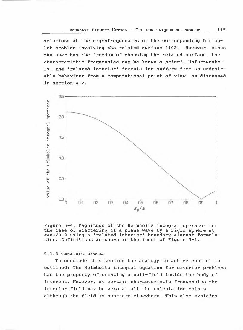
Bo u n d a r y El e m e n t M eth od - T he n o n-u n i q u e n e s s p r o b l e m 115

solutions at the eigenfrequencies of the corresponding Dirich- let problem involving the related surface [102]. However, since the user has the freedom of choosing the related surface, the characteristic frequencies may be known a priori. Unfortunate­ly, the 'related interior1 formulation suffers from an undesir­able behaviour from a computational point of view, as discussed in section 4.2.

oUaJw<1)ao<T3a>oc

•H

Ni->

<D22<D

•UU-lo<1><0>

Figure 5-6. Magnitude of the Helmholtz integral operator for the case of scattering of a plane wave by a rigid sphere at ka«jr/0.9 using a 'related interior' boundary element formula­tion. Definitions as shown in the inset of Figure 5-1.

5.1.3 CONCLUDING REMARKSTo conclude this section the analogy to active control is

outlined: The Helmholtz integral equation for exterior problems has the property of creating a null-field inside the body of interest. However, at certain characteristic frequencies the interior field may be zero at all the calculation points, although the field is non-zero elsewhere. This also explains

116 T he Bo u n d a r y E l e m ent m e t h o d for So un d F ield C a l c u l a t i o n s

why fictitious eigenfrequencies does not occur for interior problems, since in this case a null-field on the outer surface ensures a null-field overall outside S. In the next section it will be shown how this analogy may also be used to explain the problem of how to choose the so-called CHIEF points.

5.2 THE COMBINED HELMHOLTZ INTEGRAL EQUATION FORMULATIONThe Combined Helmholtz Integral Equation Formulation

(CHIEF) proposed by Schenck [78] combines the surface Helmholtz integral formulation with the interior Helmholtz integral formulation. The idea is to add a relatively small number of extra equations to the quadratic set of linear equations obtained by the surface Helmholtz integral formulation for the exterior problem. An extra equation is provided by requiring the interior formulation to be satisfied at an interior point. These points are termed CHIEF points. Using the active control analogy, the procedure is to place additional error microphones inside S in order to ensure a null-field overall inside S. This analogy also demonstrates the main problem using the CHIEF method: If the CHIEF point is placed on a nodal surface inside S, for instance at (p,zp) = (0,0.5) for the case considered in Figure 5-4, no additional constraint is obtained, and a non­zero field may still exist inside S. A numerical demonstration of this will be given in section 5.5. The term 'a good CHIEF point' is used for a CHIEF point, which really add an addi­tional constraint to the original system of equations, whereas the term 'a bad CHIEF point' is used for a CHIEF point, which does not add an additional constraint to the original system of equations.

Thus, there are two main problems using the CHIEF method:a) the determination of the number of good CHIEF points needed

to ensure a unique solution,b) and how to choose good CHIEF points.The problem of choosing good CHIEF points is coplicated by the fact that at higher frequencies the nodal surfaces of the corresponding interior problem generally are closely spaced.

Normally, the approach would be to distribute a number of

b o u n d a r y Ele m e n t M eth od - T he n o n -u n i q u e n e s s p r o b l e m 117

CHIEF points arbitrarily inside S hoping, that a sufficient number of CHIEF points will turn out as good. The resulting overdetermined set of equations is then solved in the least squares sense. The least squares solution of an overdetermined set of equations is discussed in chapter 6. The quality of the solution obtained may be estimated either by examining the Helmholtz integral operator [83] or the condition number of the coefficient matrix. The condition number is introduced in section 6.2.

5.3 THE BURTON AND MILLER METHODDue to the above mentioned problems with the CHIEF method,

several authors have adopted the Burton and Miller integral equation formulation [13]. The approach is to combine the Helmholtz integral equation with its normal derivative taken at P:

where np is the unit normal vector at P, and all other symbols are as defined in equation (2.26). Thus, equation (5.3) is multiplied with a constant and added to equation (2.26). The multiplicative constant has been a matter of interest [62,63, 97]. For real wave numbers it has been found [63,73] that the imaginary value i/k produces good results.

The main problem with the application of equation (5.3) for numerical calculations is that equation (5.3) contains a integral with a high order singularity. The evaluation of this so-called hypersingular integral is computational inefficient [13,22], and some regularization techniques are suitable for planar elements only [62,97]. For higher order elements certain conditions on the smoothness of the acoustic variables must be assumed a priori as explained in details in Chien [22]. In order to satisfy these conditions the collocation points must usually be placed inside each element [106], where the normal derivative of equation (5.3) is unique. (As discussed in para­graph 4.4.5 the normal direction is seldom unique at the

dG(R)dnp

3PZ(P)dnp

(5.3)

118 THE BOUNDARY ELEMENT METHOD FOR SOUND FIELD CALCULATIONS

intersection of two or several elements.) For three-dimensional implementations all this leads to a much larger amount of consumed time and storage. Recently a 'truncated' implementa­tion of the Burton and Miller method has been reported [36-37]. Here equation (5.3) was only applied at the local origins of quadratic isoparametric elements, where the normal direction is unique. Hence, the extra amount of work for this 'truncated' Burton and Miller formulation, which seems to be adequate to ensure uniqueness, was only about 35% compared to the standard surface Helmholtz integral formulation [37].

In order to conclude the discussion above it may be stated that although the Burton and Miller method may be proven to be a theoretically robust formulation for all frequencies [13,111] it is neither computationally efficient nor easy to implement in practice. However, it should be noted that equation (5.3) is the preferable method for calculating radiation and scattering for thin-walled shapes [54,60,108], since the standard surface Helmholtz integral equation method can not be applied directly in this case.

The Burton and Miller method has not been examined in this study.

5.4 OTHER METHODS TO OVERCOME THE NON-UNIQUENESS PROBLEMIn this section some of the other methods of dealing with

the nouniqueness problem will be outlined. Alternative numeri­cal formulations, which are not based on a direct solution of the Helmholtz integral equation have been proposed [43,47,57, 66,104]. The idea of these methods is generally to place a number of sources inside the body, and then to determine the strength of these sources by matching the boundary conditions in a variational sence on the surface S. The problem of apply­ing these methods to general shapes lies in the selection of the source points. Furthermore, these methods are not suited for slender bodies or bodies having sharp edges and/or corners, and they often have the same undesirable computational charac­teristics of the interior Helmholtz integral equation formula­tion discussed in section 4.2, due to the lack of diagonal

Bo u n d a r y El e m e n t M eth od - T he n o n -u n i q u e n e s s p r o b l e m 119

dominance in the resulting matrix of coefficients [47,78,94]. The author finds that a more comprehensive description of these methods is beyond the scope of this text. Hence, only formula­tions based on the Helmholtz integral equation are outlined in the following.

In a formulation due to Piaszyk and Klosner [68] a CHIEFpoint is placed outside the surface. Since the exterior fieldis unknown at the outset, this approach requires an iterative procedure to obtain a solution. The convergence of this pro­cedure was not proved rigorously. Another CHIEF method known as the 'enhanced' CHIEF method [89] or as SuperCHIEF [79] requires not only the original CHIEF equation to be satisfied inside Sbut also its derivatives. The 'enhanced CHIEF method uses firstorder derivatives, whereas the SuperCHIEF method used higher order derivatives. However, if the 'enhanced' CHIEF point falls on the intersection of two nodal surfaces no additional con­straint is obtained [107]. Finally, a CHIEF method that requires the CHIEF equation and its normal derivatives to be zero in a small interior region rather than at a point has been suggested [107]. This method is expected to eliminate the non­uniqueness problem, since for the corresponding interior problem only, the desired null solution has nodal 'blocks'.This method has been termed the CHIEF-block method.

At the other end of the spectrum Cunefare, Koopmann, and Brod [30] has suggested a variant of the Burton and Miller method, in which all calculation points are placed inside the body. The advantage of this scheme is that the hypersingular integral is avoided, since in this case the integration point Q never encounters the calculation point P. This 'interior Burton and Miller approach' was termed CHI for Coupled Helmholtz Inte­grals. Unfortunately, this method suffers from the well known undesirable computational characteristic: lack of diagonal dominance of the coefficient matrix, and the formulation encounters difficulties when applied to slender bodies or bodies with sharp edges.

Finally, Ursell [103] modified the Green's function such that uniqueness was ensured. However, this approach gives rise

120 T he Bo u n d a r y E l em e n t M eth od for So un d F ield C a l c u l a t i o n s

to an infinite series which converged slowly at high fre­quencies. Jones [48] replaced the infinite series with a finite, but uniqueness could then be guaranteed only in a range of frequencies.

5.5 A BRIEF NUMERICAL STUDY OF THE CHIEF METHODAnalytically, the characteristic frequencies exist at a

discrete set of frequencies only, and the problem of character­istic frequencies would not be severe if this was the case for the numerical implementation as well. However, due the numeri­cal approximation, the standard surface Helmholtz integral equation formulation encounters problems in a range of fre­quencies around a characteristic frequency. In this frequency band the solution produced by the standard surface Helmholtz integral equation formulation is largely in error.

Consider as an example scattering of a plane wave by a rigid sphere of radius a near ka=ir, which is the first charac­teristic frequency for the sphere. The plane wave has the dimensionless magnitude one. Figure 5-7 shows the error made by the standard formulation compared to the error made by the CHIEF method with one CHIEF point in the centre of the sphere. The error is calculated as the length of the residual vector as defined in paragraph 4.6.1. For these calculations the axisym­metric integral equation formulation was used. In Figure 5-7 three cases are considered: the CHIEF method using 4 isopara­metric elements to model the generator of the sphere, the standard formulation using 4 isoparametric elements to model the generator, and the standard formulation with 6 isoparame­tric elements on the generator. Note that using 4 elements corresponds to about 2,5 elements per v/avelength, which is close to the recommended discretization for coarse calcula­tions. In this case the CHIEF point is good, and hence this calculation is believed to represent the minimal error that may be obtained with the four element discretization. The two curves for the standard formulations can be used to acces the issue of the bandwidth of characteristic frequencies mentioned. It can be seen that the solution obtained by the two standard

Bo u n d a r y E l e m e n t M eth od - T he n o n -u n i q u e n e s s p ro blem 121

formulations has large errors in a range of frequencies around the characteristic freqiency, and that generally the 4 element model is in more error than the 6 element model. It can also be seen that the actual bandwidth, in which poor solutions are obtained, depends on the accuracy demanded by the user. If, for instance, the user demands the error to be less than 0.3, which is about 3 times the error obtained using the CHIEF method, then the bandwidth of poor solutions is about 0.013 for the 4 element model, and 0.005 for the 6 element model in this case. Thus, the effect of discretization is, that for a coarse discretization a larger error is encountered than for a finer discretization, as also found in [83].

3.129 3.131 3.133 3.135 3137 3139 3141 3143 3.145 3.147 3149 31513.133 3132 3134 3136 3.138 3.140 3142 3.144 3146 3.148 3150ka

Figure 5-7. Error made by three boundary element calculations in the case of scattering of a plane wave by a rigid spherenear ka=n. ---■---, CHIEF calculation using 4 quadraticelements? ---□---, standard calculation using 4 quadraticelements; ---+--- , standard calculation, using 6 quadraticelements.

122 T he Bo u n d a r y E l em e n t M eth od for Soun d F ield Ca l c u l a t i o n s

In order to observe the effect of the 'sophistication1 of the formulations in terms of the order of the shape functions used the same problem was run using the linear elements described in paragraph 4.4.1. Figure 5-8 shows the error made by an isoparametric linear CHIEF, an isoparametric linear standard formulation , and the isoparametric quadratic formula­tion used in Figure 5-7 as well. For all formulations 13 nodes were used.

ai30 3.132 3.134 ai36 3.138 3.140 3.142 ai44 ai46 3.140 3150ka

Figure 5-8. Error made by three boundary element calculations in the case of scattering of a plane wave by a rigid spherenear ka=*. ---■ , CHIEF calculation using 12 linear elements; □---, standard calculation using 12 linear elements; 1----, standard calculation using 6 quadratic elements.

It can be seen from the figure that the conclusions drawn considering the effect of discretization also holds when considering the effect of 'sophistication* of the methods: the more 'sophisticated' standard quadratic formulation performs generally better near a characteristic frequency than the

Bo u n d a r y E l e m e n t M e t h o d - T h e n o n-u n i q u e n e s s p r o b l e m 123

linear formulation with the same number of nodes.Similary, the nodal surfaces inside the body has a certain

spatial bandwidth due to the numerical modelling. Since an investigation of the spatial bandwidth leads to conclusions analogous to the conclusions drawn for the frequency bandwidth case [83], this effect is merely demonstrated in the case of scattering of a plane wave by a rigid sphere at ka=6.2832, which was the case also considered in Figure 5-4. Figure 5-9 shows the error as a function of the location of the CHIEF point zp as shown in the inset in the figure. Evidently, the CHIEF point should not be placed near the nodal surface or near the boundary surface. This calculation was carried out using a 29 element isoparametric linear formulation.

Figure 5-9. Error made by a 30 node isoparametric linear CHIEF calculation in the case of scattering of a plane wave by a rigid sphere at ka=6.2832. The error is shown as a function of the location of the CHIEF point as defined in the inset in Figure 5-1.

124 T he Bo u n d a r y El e m e n t M e th od f o r So u n d F ield Ca l c u l a t i o n s

To conclude this section it can be stated that due to the numerical treatment, the solution of the standard Helmholtz integral equation fails in a band around the characteristic frequencies. Likewise, a spatial bandwidth is observed for the locations at which the CHIEF points are 'bad'. Although these bands theoretically may be narrowed as much as the user wishes by increasing the number of elements, this strategy to overcome the non-uniqueness problem leads to an enormous amount of time and storage required. The problem of characteristic frequencies and nodal surfaces is further complicated by the fact that at higher frequencies the number of characteristic frequencies per octave increases and the spacing between the nodal surfaces decreases.

Bo u n d a r y El e m e n t M e t h o d - s o l u t i o n o f l i n e a r e q u a t i o n s 125

6. SO LU T IO N OF LINEAR ALGEBRAIC EQ U AT IO N S

In chapter 4 the Helmholtz Integral Equation was trans­formed into the matrix equation

(C-H) p = Gv + 47rpJ . (6 .1)

Thus the distribution of the pressure p and the normal velocity v is replaced by a finite number of nodal values, of which either p or v is known at each node. Alternatively, an impe­dance relation may be known:

P = -Zv , (6 .2)

where Z is an impedance matrix; the negative sign is due to the fact that the velocity is calculated along the outward normal to the surface. For a locally reacting surface Z has values in the diagonal only. Thus, when introducing the boundary condi­tions, equation (6.1) may be reduced to

A com x com _ com (6.3)

where A is a MxM matrix, and x and b are vectors of length M. M is the number of acoustical nodes. The superscript com in equation (6.3) refers to the fact, that the quantities are complex:

A com = A re + i A ^ ,^ com = X re + i x ^ , (6.4a,b,c)com = b re + ib*" .

The solution of a complex set of equations may either be found using a solution algoritm working with complex numbers or - as is the case in this work - by transformation of the complex set of equations (equation (6.3)) into an equivalent 2M*2M set of equations

imA r e - A

A im A rex re b rex ±m b im

(6.5)

where all elements are real numbers. Although the latter method requires twice the storage of the former, this method has been

126 T h e Bo u n d a r y E le m e n t M eth od for So u n d F ield Ca l c u l a t i o n s

chosen for the present work. This is mainly because many well- documented standard algoritms with program listings for solving a real set of equations are available [33,70], and secondly because handling complex number is quite difficult in Pascal, which is the programming language used in this project.

Keeping the transformation of a complex set of equations (equation (6.3)) into a real set of equations (equation (6.5)) in mind, the real system of equations

Ax = b (6.6)

is considered in the following.The purpose of this chapter is not to discuss the solution

of equation (6.6) in detail. The problem of solving a set of equations is the issue of numerous numerical methods, and are consequently well described in the literature. The author recommends Press et al. [70] for a short introduction to the subject, and Golub and Van Loan [39] for a more detailed treatment. In this chapter the three different algoritms used in this project for solving equation (6.6) will merely be outlined. The matrices produced by boundary element formula­tions are generally neither band limited nor symmetric, and hence general algorithms for solving a set of equations must be used.

The 'text-book' method of solving equation (6.6) is the Gauss-Jordan elimination, which implies the determination of the inverse of A by the means of 'row-operations'. A 'row- operation' is the replacement of a row in A by a linear combination of the row it selv and any other row.

However, a full inversion as obtained using the Gauss- Jordan elimination of A is not required for finding the unknown vector x, and hence modern and more efficient methods of solving a set of equations brings A to a form from which the solution of the set of equations is more easily obtained. This process is termed factorization or decomposition of A.

The factorization of A is independent of the right-hand side of equation (6.6), and hence the factorization of A may be reused for different right-hand sides. This feature is useful

Bo u n d a r y E lem e n t M eth od - So l u t i o n o f l i n e a r e q u a t i o n s 127

for several boundary element calculations e.g. solution of scattering problems involving several angles of incidence. Gauss-Jordan elimination requires the right-hand side to be known in advance, and is therefore not suitable for iterative methods, where the right-hand side depends on the result of the previous iteration. Iteration will be used in chapter 7.

Two other operations frequently carried out when solving a linear set of equations numerically are the interchanging of two rows or two columns of A. Interchanging two rows of A and the right-hand side of the equation simply corresponds to writing the system of equations in a different order. However, the proper interchanging of rows is vital for the numerical stabitity of the LU factorization to be described in section 6.1, and is termed partial pivoting or row pivoting [70]. For the so-called QR factorization to be described in section 6.3 interchanging of columns - column pivoting - may be performed in order to stabilize the algorithm numerically. In this case the rows of the unknown vector x is interchanged corresponding­ly, and the solution must be 'unscrambled1 to the original order afterwards. For more details about pivoting refer to e.g. Golub [39].

The number of floating point operations (flops) required by an algoritm is often used for measuring the efficiency when comparing different factorization algoritms. A flop is either a multiplication or an addition. Gauss-Jordan elimination of a NxN matrix requires 2N3 flops, for instance.

The most common factorization method used to solve a system of equations is the LU factorization, which will be described in the next section. However, it appears that alternative factorization methods may advantageously be used near a charac­teristic frequency as will be demonstrated in section 6.4. Two such factorization methods, the singular value decomposition, and the QR factorization, will be outlined in section 6.2 and section 6.3 respectively.

128 T he Bo u n d a r y E lem e n t M eth od for So u n d F ield C a l c u l a t i o n s

6.1 LU FACTORIZATIONIf A is quadratic (NxN) and regular (i.e. not singular) the

following factorization can always be made [39]:

A = L U ,

where I# is a lower triangular matrix:

L =

and U is an upper triangular matrix:

' 1 0 0 0 '221 1 0 0■*31 -*32 1 0■*41 -*42 -*43 1

(6.7)

(6 .8 )

U =

U11 u i2 u 13 “ 140 U 22 “ 23 “ 240 0 “ 33 “ 340 0 0 “44

(6.9)

The factorization is shown for a 4x4 matrix but is of course general for any NxN matrix N-2,3,4,...

Once the LU factorization of A is performed, the solution of equation (6.6) is easily obtained by the following two steps. First solve

and then

Ly = b

Ux = y .

( 6 . 1 0 )

(6 . 1 1 )

Equation (6.10) is easily solved by a technique called forward substitution:

y i = i>!i-1

y± = b ± ~ Y , 2± j y jj-i

(6 .1 2)

and equation (6.11) by back substitution

Bo u n d a r y E lem e n t M eth od - So l u t i o n o f l i n e a r e q u a t i o n s 129

x n =

x i =

y NU NN

1U±±

(6.13)N

y±- E uaxjj * i + i

The calculation of L and U requires 2/3N2 flops, whereas a total of 2N2 flops are required by equations (6.12) and (6.13) for each right-hand side. Hence, for large systems (say, W>100) and relatively few right-hand sides LU factorization is about three times as efficient as Gauss-Jordan elimination.

As stated in chapter 5 a solution to a system with more equations than unknowns might be wanted in order to ensure uniqueness of the solution. In this case the linear least squares solution is of interest. The linear least squares solution is the solution that comes closest to satisfing all equations silmutaneously in the sence that the sum of the squares of the differences between the left and right-hand side of equation (6.6) is minimized. The linear least squares solution may be shown to be the solution of the normal equa­tions :

(AtA) x = (ATb) , (6.14)

where Ar denotes the transpose of A. However, equation (6.14) is not generally the best way to find least squares solutions[70]. Note that ATA is symmetric, and hence almost half of the work may be saved in computing ATA. Furthermore, a specialized and time saving factorization scheme, which takes advantage of the symmetry of the matrix may by used to compute the solution to the normal equations. One such method is the Cholesky factorization [39].

6.2 THE SINGULAR VALUE DECOMPOSITIONBy the transformation of the integral equation to a linear

set of equations the problem of characteristic frequencies appears as an ill-conditioning of the coefficient matrix Acom. The condition number k may be roughly described as the factor a

130 THE BOUNDARY ELEMENT METHOD FOR SOUND FIELD CALCULATIONS

disturbance of an element in the matrix Acom or the right-hand side bcom may be multiplied with in the solution vector xcom. Thus the matrix is ill-conditioned if the condition number is large, and if the condition number is infinite the matrix is singular. As the elements of Aaom are the results of approxi­mations (discretization and numerical integration), the un­certainty related to these elements are usually much larger than the internal machine precision.

In handling singular/ill-conditioned matrices the Singular Value Decomposition (SVD) is often considered the ultimate tool, see e.g. Press et al.[70]. The Singular Value Decompo­sition of the real square NxN matrix A of equation (6.6) is defined as

A = U W V T . (6.15)

This decomposition is always possible [39,70], and programs to perform the SVD are available both for main-frames and for PC's (routines are listed e.g. in Press et al.[70]). The matrices U and V are orthogonal, i.e.

Nr „ „ = c l<k<Nuikuln 6 kn • 1<71<N1=1

N •V v x l<k<NZs jk jn 5kn ' i<n<N7=1

(6.16a,b)

where uik denotes the element in row i and column k of matrix U, and 8 is the Kronecker delta. W is a diagonal matrix, and the values wjj (or shortly wj) in the diagonal of W are called the singular values. Without loss of generality the columns of the matrices U, V, and W may be arranged in order of descending Wj's, so that wx is the largest element and wN is the smallest. Since U and V are orthogonal their inverses equal their trans­poses, and the inverse of A is thus

A -1 = V- [diagfl/wry) ] • U T . (6.17)

Analytically, this formula behaves well if none of the w^'s are zero, but numerical problems arise if one or several of the

Bo u n d a r y E l e m ent M eth od - So l u t i o n of l i n e a r e q u a t i o n s 131

w^'s are small compared to the accuracy of the elements of A. The condition number k of a matrix is defined as the ratio Wi/WN' and as previously mentioned the matrix is said to be ill-conditioned/singular if this ratio is large/infinite.

In order to investigate the properties of the SVD further, it is convenient to regard A as the matrix of a linear mapping:

y = Ax , (6.18)

i.e. the vector x is mapped on to the vector y by eguation (6.18). The columns in U and V calculated by a SVD are con­nected by the simple relation

Avj = WjUj . ( 6 . 1 9 )

Any vector xgEn may be expressed by the columns of V:

* = £lv i + t 2v 2 + * • - + ^ N V N / (6.20)

and the vector y onto which x is mapped by equation (6.18) maybe expressed using equation (6.19) and equation (6.20):

N

y = £ tjwjuj • (6.2i)j =i

Considering equation (6.19) the Wj's may thus be regarded as the magnification of the 1s when mapped onto the correspon­ding Uj's. Thus the Wj%s are, in some sense similar to a trans­fer function. If A is regular y will go through all possible combinations of the columns of U as x goes through all possiblecombinations of the columns of V, given by equation (6.20).Consequently the columns of V is an orthogonal basis for the solution space of A, and the columns of U is an orthogonal basis for the range of A . Range refers to what may be reached by the linear mapping defined by A.

If A is singular then one or several of the wj *s are zeroand the corresponding last column(s) of V are called singular vectors and are by equation (6.19) mapped on to the zero- vector:

Avj = 0 . ( 6 . 2 2 )

In this case A is said to be rank deficient, and if the rank of

132 T he Bo u n d a r y E l e m e n t M eth od f o r Soun d F ield Ca l c u l a t i o n s

A is R, then the last N-R of the wj's would be zero. In that case two additional subspaces are needed in the discussion of the mapping. The last N-R columns of V are called the null space of A since they are mapped into the zero-vector, and the corresponding last N-R columns of U are called the orthogonal complement of A, since this vector space may not be reached by the mapping defined by equation (6.18). The solution space of A is then spanned by the first R columns of V, and the range of A by the first R columns of C7. These properties are summarized in table 5:

name basis vectors dimensionrange U1 / / • • / UR R

orthog. compl. UR+1' • * * 'UN N-Rsolution space vn , v9, . . . , Vr R

null space VR+1'-- ' VN N-R

Table 5: The connection between the four fundamental subspaces and the singular value decomposition.

If A is the coefficient matrix of a system of equations to be solved for a known right-hand side b, such as

Ax = b , (6.23)

then A being singular corresponds to one of tv/o alternatives: Either the system of equations has no solution, which is b is not in the range of A, or the system of equations has one or several infinities of solutions, since in this case any combi­nation of the zero-vectors (vR+1,...,vN) may be added to a specific solution. In the latter case b is in the range of A, and may be expressed as a linear combination of the first R columns of A.

Turning now to the BEM, it is a fact that a solution is known to exist at the characteristic frequencies when using the Helmholtz integral equation, which is in contrast to e.g. the simple source formulation [78]. Hence, the latter of the above alternative must be the one encountered in the present case.The number of zero wj elements is, as previously stated, the

Bo u n d a r y E l e m e n t M eth od - So l u t i o n o f l i n e a r e q u a t i o n s 133

rank deficiency of the matrix A and is also the number of missing linearly independent equations that must be added in order to obtain a system where the number of linearly inde­pendent equations equals the number of unknowns. Thus the problem is to add additional constraints to the system of equations in order to obtain an unique solution out of the infinity many solutions to the sinqular system of equations.

Numerically, an exact singular matrix seldom occurs, and in fact it has been proved [34] that an exact singular matrix never occurs in boundary element matrices. However, the situ­ation described above presents it self in the shape of an ill- conditioned matrix. The numerical rank deficiency of a matrix may be defined as the number of 1s below a certain value. If equation (6.17) is used without modifications at a characteris­tic frequency, the solution vector may be wandering off towards infinity in a direction of an almost singular vector, or, in the case of a rank deficiency higher than one, any combination of the singular vectors.

Note that the SVD may also be used in the case of an MxN matrix (M>N). In this case U is a MxN column-orthogonal matrix, and the matrices V and W are both NxN. The solution produced by the SVD is the linear least squares solution. The generalized condition number is still defined as the ratio A matrixfor which the number of rows does not equal the number of columns is termed a rectangular matrix. In terms of accuracy the SVD is more favourable than the traditional least-squares procedure using AVA, since the matrix ATA has the condition number k 2 if the rectangular matrix A has the condition numberAC .

As demonstrated above, the singular value decomposition is the ultimate choice in terms of obtaining information about the set of equations. The price payed is in terms of effciency: In order to solve an NxN system 12«N3 flops are required. It will be demonstrated in section 6.4 that the information useful for boundary element calculations consists of the smallest singular values and the corresponding almost singular vectors. This information may be obtained considerably cheaper in terms of

134 T he Bo u n d a r y El e m e n t M eth od f o r Sou n d F ield Ca l c u l a t i o n s

flops using a superstructure based on the QR-factorization to be described in the next section.

6.3 THE QR-FACTORIZATIONThe matrix A of equation (6.6) may also be written as

A = QR , (6.14)

where Q is an orthogonal NxN matrix and R is upper triangular. Hence, the set of equations can be solved in two steps:

y = Q Tb (6.15)

and

Rx = y , (6.26)

where backsubstitution as in equation (6.13) is used to solve equation (6.26). The Rank Revealing QR (RRQR) factorization is a special QR factorization, for which the column pivoting is organized in a way which ensures that the numerical rank, and hence ill-conditioning, is revealed by producing good estimates of the smallest singular values. Furthermore, good estimationsof the singular vectors are also obtained. The algorithmicdetails and proofs may be found in [16). Here it suffices to say that the coefficient matrices produced by the boundary element method are well-suited for the RRQR algorithm, and that in all cases studied by the author, the RRQR factorization has provided qualitatively the same singular values and singular vectors as the singular value decomposition.

However, the RRQR factorization is much more efficient than the singular value decomposition. In order to compute a QR factorization of an NxN matrix 4/3»N3 flops are required. Although this number of flops is twice the number of flops for the LU-factorization, the QR factorization tends to be as effi­cient as the LU factorization in practice [39]. This is because the QR algorithm adresses the elements of A in the same order as they are stored in the computer, and thus reduces the memory traffic in the computer. The rank revealing superstructure on

Bo u n d a r y El e m e n t M eth od - So l u t i o n o f l i n e a r e q u a t i o n s 135

the QR algorithm requires only in the order of N2 flops for the estimation of each small singular value, and the corresponding singular vector. Hence the extra amount of work due to the rank revealing part is vanishing for large systems of equations with a small rank deficiency, compared to the work of the QR factorization.

If the matrix A is overdetermined (MxN where M>N), the QR factorization produces the linear least squares solution. In this case Q is an MxM orthogonal matrix and R is an MxN upper triangular matrix. Both in respect to accuracy and the time consumed, the QR factorization is preferable for solving the linear least squares problem when M-N is small compared to N , as usually is the case for boundary element calculations.

Finally, another important feature of the QR factorization should be mentioned: If the QR factorization of e.g. a square (NxN) system is known, the QR factorization may be updated rather than recalculated if more equations are added to the system [39]. For boundary element calculations this feature is very useful: If ill-conditioning has been found by the RRQR factorization due to the pressence of a nearby characteristic frequency, addition of further equations to the original system of equations will be required. This could be done by the CHIEF method or by a related approach, see sections 5.2 and 5.4. In this case a new QR factorization need not to be calculated from the start. The updating of the QR factorization requires an order less of flops than the QR factorization it self, and hence the time spend to update the QR factorization is vanish­ing for a large system of equations with a small number of extra equations added, which generally is the case using CHIEF or a related approach.

136 T he Bo u n d a r y E le m e n t M e t h o d for So u n d F ield C a l c u l a t i o n s

6.4 USING RANK REVEALING FACTORIZATIONS WITH METHODS TO OVERCOME THE NONUNIQUENESS PROBLEMIn section 5.2 it was concluded that there were two major

problems related to the CHIEF method:a) the determination of the number of good CHIEF points needed

to ensure a unique solution,b) and how to determine whether a CHIEF point is good.In this section it will be demonstated how both problem may be overcome by the use of rank revealing factorizations. For simplicity the approach will be described using the original CHIEF approach, although the scheme presented here is valid for the enhanced CHIEF [89], the SuperCHIEF [79], and the CHIEF- block [107] methods without modifications. For clarity the theory is described using the singular value decomposition although the rank revealing QR factorization is preferable from a computational point of wiev as discussed in sections 6.2 and 6.3. All calculations presented here has been re-calculated using the RRQR factorization and the same results were found.

6.4.1 USING THE SINGULAR VALUE DECOMPOSITION IN BOUNDARY ELEMEMT CALCU­LATIONS

The theory for the singular value decomposition in section6.2 was discussed for the case of a real matrix A. The handling of the complex boundary element method (BEM) coefficient matrix in equation (6.3) has been done by rewriting the complex system of equations in equation (6.3) as the real system of equations in equation (6.5). Now, if x0=x0ro+ix0iin is a singular vector so that

A re -A 210 A re

x,

X

re0im0

= 0 (6.27)

then it immediately follows that -x0I+ix0R is a singular vector as well, and this vector is evidently orthogonal to x0=XoR+ix0I. It can be shown that the singular values of the matrix in equation (6.5) always appear as pairs of the same value due to the special structure of the 2Mx2M matrix, and

Bo u n d a r y El e m e n t M eth od - So l u t i o n o f l i n e a r e q u a t i o n s 137

that the two columns in both U and V , corresponding to the two identical w^'s, have the property mentioned above. In the following examples only one value of the pair of wj's is shown. In order to investigate the behaviour of the singular values (the Wj's) near a fictitious eigenfrequency, the SVD has been performed on the square BEM coefficient matrix in the case of a rigid sphere. The axisymmetry of the geometry in the presented examples has been exploited, and hence the test cases have been calculated by means of an axisymmetric boundary element formu­lation, where only the generator of the body has been dis­cretized. The generator of the sphere was divided into 19 isoparametric linear elements.

One of the important properties of the SVD is demonstrated in figure 6.1, which shows the singular values of the BEM coefficient matrix in a frequency range near the first charac­teristic frequency at ka=n. From the figure it is evident that the first 19 singular values are practically constant in the range of ka=3.128 to ka=3.156, whereas the last singular value shows a strong dependence of the distance to the characteristic frequency. Since the first singular value w± is almost constant in this frequency range, the condition number k = w 1/ w m (M=20) is inversely proportional to the last singular value and thus becomes large as the frequency approaches the characteristic frequency. Hence the problem of characteristic frequencies is directly reflected in the last singular value in this case. Since only one singular value becomes small at ka=n, only one good CHIEF point is needed to add the sufficient constraint to the system of equations. Accordingly, the condition number calculated by the SVD for the overdetermined system of equa­tions, produced by the BEM coefficient matrix with a CHIEF point in the centre of the sphere, is k = 2.6, which is very close to the best possible theoretical value, unity.

138 T h e Bo u n d a r y E le m e n t M eth od for So u n d F ield Ca l c u l a t i o n s

Figure 6.1. The 20 singular values of the boundary element coefficient matrix for a 20 node discretization of a rigid sphere near the first characteristic frequency at ka=n.

6.4.2 NUMERICAL RANKAs briefly mentioned in section 6.2, an exact singular

matrix practically never occurs in boundary element calcula­tions [34]. Instead the problem of characteristic frequencies is reflected in an ill-conditioning of the boundary element coefficient matrix. Hence, a threshold for the wj's under which the matrix is said to be numerically rank deficient must be chosen. In order to investigate the connection between the smallest singular value and the error made by the BEM formu­lation without any CHIEF points the following testcase has been calculated. The error made by the isoparametric linear BEM formulation in the case of scattering of a plane wave of unit magnitude by a rigid sphere, and the smallest singular value have been calculated. The results are plotted as functions of the dimensionless wavenumber ka in Figure 6-2.

Bo u n d a r y E lem e n t M e t h o d - So l u t i o n of l i n e a r eq u a t i o n s 139

ka

Figure 6-2. Solution error and the smallest singular value near the first characteristic frequency at ka=ir. □, Smallest singu­lar value for 20 node discretization; *, smallest singularvalue for 40 node discretization; --------- , solution error for20 node discretization; -------- , solution error for 40 nodediscretization.

The error is as usual calculated as the length of the residual vector - the residual vector being the vector containing the difference between the analytical solution and the BEM solution at the nodes. For this figure two BEM calculations have been made: one using a 20 node discretization (the same as used for Figure 6-1), and one using a 40 node discretization.

The figure shows that for both discretizations, the smallest singular values are practically identical, whereas the error depends strongly on the discretization. This may be explained by the close relation between the smallest singular value and the condition number. As mentioned previously, the condition number may be regarded as the 'blow-up' factor for the error due to the approximations made by the BEM formula­tion, and evidently the degree of approximation is larger for

140 T h e Bo u n d a r y Ele m e n t M e t h o d for So u n d F ield Cal c u l a t i o n s

the 20 node formulation than for the 40 node formulation.Hence, although the smallest singular value is the same in the two situations, the resulting error is not. However, the smallest singular value obviously proves to be a good estimate of the error and thus it is possible to use the smallest singular value as an error indicator. Thus it is possible to choose a threshold for the singular values, and improve the standard BEM formulation e.g. by adding CHIEF points if this threshold is crossed. As mentioned above, the resulting error is not a function of the smallest singular value only, and hence the threshold should be chosen for each actual implemen­tation of the Helmholtz integral equation specifically. For any practical implementation the ratio of v/avelength to element could be kept size constant, and the error made by this par­ticular implementation could be examined for cases where the non-uniqueness problem does not occur. The threshold could then be defined by examining the smallest singular value for the implementation as the frequency is moved close to a character­istic frequency. The threshold would then be the largest of the smallest singular values in the band of frequency band where the error is unacceptably high compared to the level found in the first experiment.

6.4.3 adding a chief pointOnce the number of good CHIEF points needed to pick out the

correct solution to the problem has been determined by inspect­ing the singular values of the BEM coefficient matrix, it becomes important to be able to estimate the quality of a CHIEF point. Note that if the complex system of equations has been transformed to a real system by equation (6.5), a CHIEF point provides two independent equations to be satisfied along with the standard BEM coefficient matrix corresponding to the two singular vectors shown to exist in paragraph 6.4.2 for the pair of singular values.

The SVD provides a very good tool for deciding whether a CHIEF point is good: the singular vectors. When a matrix A is rank-one deficient, that is, when the smallest singular value

Bo u n d a r y E l e m e n t M eth od - So l u t i o n o f l i n e a r e q u a t i o n s 141

is zero, any constant times the singular vector may be added to a specific solution without altering the righthand side. Consider for simplicity the real system of equations

Ax = b (=A(x+tx0)) ; teR , (6.28)

where x0 is a singular vector. In order to pick out a solution from this infinity of solutions an extra equation may be added by means of a CHIEF point to impose the necessary constraint on the parameter t. This results in a rectangular system of equations. If the extra equation adds the necessary constraint, that is, the CHIEF point is good, then the rectangular system is non-singular. This implies that the singular vector xQ of equation (6.28) is not a singular vector for the rectangular system

A

C

aex ' x0 * (6.29b)

since Ax0 =0. If equation (6.29b) is true then the rectangular system of equations is non-singular, and the solution may be found as the least-squares solution of the rectangular system. In practice the left-hand side must be greater than a certain threshold, of course.

The lefthand side of equation (6.29b) may be used as a quality indicator of the extra equation, since a small product implies that no additional constraint has been obtained.

The theory described above is also valid for the case of the 2MX.2M real system transformed from the complex BEM coeffi­cient matrix. Here the combination of two singular vectors corresponding to the pair of singular values is to be found from the two extra equations added by a CHIEF point. Due to the special symmetry of the equations, the largest of the dot products of an extra equation and the singular vector may be used as the quality indicator.

(6.29a)

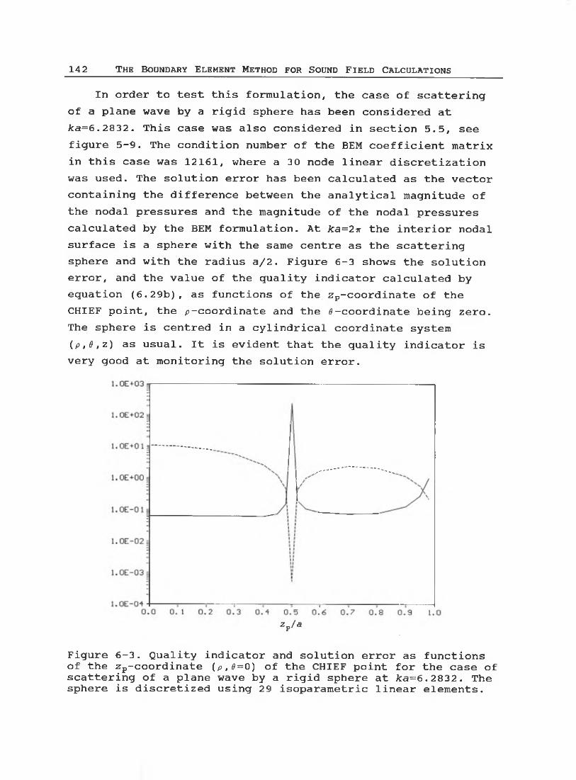
142 THE BOUNDARY ELEMENT METHOD FOR SOUND FIELD CALCULATIONS

In order to test this formulation, the case of scattering of a plane wave by a rigid sphere has been considered at ka=6.2832. This case was also considered in section 5.5, see figure 5-9. The condition number of the BEM coefficient matrix in this case was 12161, where a 30 node linear discretization was used. The solution error has been calculated as the vector containing the difference between the analytical magnitude of the nodal pressures and the magnitude of the nodal pressures calculated by the BEM formulation. At ka=2n the interior nodal surface is a sphere with the same centre as the scattering sphere and with the radius a/2. Figure 6-3 shows the solution error, and the value of the quality indicator calculated by equation (6.29b), as functions of the zp-coordinate of the CHIEF point, the p-coordinate and the 0-coordinate being zero. The sphere is centred in a cylindrical coordinate system (p,0,z) as usual. It is evident that the quality indicator is very good at monitoring the solution error.

z?/a

Figure 6-3. Quality indicator and solution error as functions of the Zp-coordinate (p,9=0) of the CHIEF point for the case of scattering of a plane wave by a rigid sphere at /ca=6.2832. The sphere is discretized using 29 isoparametric linear elements.

Bo u n d a r y El e m e n t M eth od - So l u t i o n of li n e a r e q u a t i o n s 143

6.4.4 THE SINGULAR VALUE DECOMPOSITION AT HIGHER FREQUENCIESAt higher frequencies the non-uniqueness problem becomes

more severe due to the close spacing of the characteristic frequencies and due to the associated 'bandwidth' as discussed in section 5.5. A situation where the bands of bad solutions no longer are distinct and the solution is corrupted by two or more characteristic frequencies near any chosen frequency may very well be encountered. This situation is reflected in two or more small singular values calculated by the SVD with corre­sponding singular vectors, and the numerical rank deficiency of the BEM coefficient matrix is thus greater than one. Now, the strategy is to choose a CHIEF point that satisfies equation (6.29b) for each singular vector, and thereby decrease the rank deficiency by one in the resulting rectangular matrix. When this has been done for all singular vectors, the resulting rectangular matrix is fully ranked, that is, the rank equals the column dimension, and thus the non-uniqueness problem is solved. Note that each CHIEF point need to concern only one singular vector in order to decrease the rank deficiency. Thus it is only required that equation (6.29b) is fulfilled for this particular singular vector, and not for any other singular vector, because they are taken care of by other CHIEF points.

In order to generate a higher rank deficiency, scattering of a plane wave with unit magnitude from a rigid sphere for the characteristic frequency at ka=15.0397 has been considered. The generator of the sphere has been discretized into 79 isoparametric linear elements. In this case two singular values become very small due to the presence of another fictitious eigenfrequency at ka=15.0335, which is reflected in the condi­tion number k=w1/wm=24 66, and the following ratios w1/wM_1=310 and w1/wM_2=:9.1. Thus the numerical rank deficiency of the BEM coefficient matrix is two. Figure 6-4 shows the magnitude of the pressure on the surface as a function of the angle defined in the small inset in the figure. It is evident that in this case two 'good' CHIEF points are required to obtain an accurate solution, since the difference between the curves representing the analytical solution and the BEM solution using two CHIEF

144 T h e Bo u n d a r y El e m e n t M e t h o d for So un d F ield Ca l c u l a t i o n s

points is hardly noticeable. The CHIEF points have been selected with respect to the quality indicator under consider­ation.

angle w (degrees)

Figure 6-4. Scattering by a rigid sphere at /ca=15.0397 wherethe numerical rank deficiency is two-------- , analyticalsolution; ------- , BEM solution using one CHIEF point; ....BEM solution using two CHIEF points.

6.4.5 CONCLUDING REMARKSIn this section the non-uniqueness problem of the exterior

BEM formulation has been investigated by means of the Singular Value Decomposition (SVD) . It has been shown that the rank deficiency of the BEM coefficient matrix at characteristic frequencies may be revealed by the SVD.

Furthermore, it has been shown that due to the 'bandwidth' of the characteristic frequencies the rank deficiency of the BEM coefficient matrix may be greater than one when two or

Bo u n d a r y E l e m e n t M e t h o d - S o l u t i o n o f l i n e a r e q u a t i o n s 145

several characteristic frequencies are near the frequency of interest.

The number of good CHIEF points needed to obtain a unique solution equals the rank deficiency of the BEM coefficient matrix, and it has been shown that by making use of the singu­lar vectors obtained by the SVD the quality of the CHIEF points can be determined reliably.

As mentioned in the beginning of section 6.4, the same information may be obtained using the far more efficient RRQR factorization. The extra cost with respect to computation time comsumed of the RRQR factorization is insignificant compared to the cost of the LU-decomposition, which is the standard method of solving a fully populated set of equations.

This approach may also be applied to more advanced methods to overcome the non-uniqueness problem.

It must be emphasized that the test cases presented in this section concern an axisymmetric model, where the rank defi­ciency problem is less severe than in a general three-dimen­sional formulation. However, the method is valid for general three-dimensional formulations as well. A paper describing this work has been accepted for publication [52].

146 T he Bo u n d a r y E l em e n t M eth od for Soun d F ield Ca l c u l a t i o n s

7. APPLICATION OF THE B O U N D A R Y ELEMENT

M E T H O D TO INVEST IGATION OF STAN DARD

C O N D EN SER M IC R O P H O N E S

Since 1989 an extensive work on free-field reciprocity calibra­tion has been carried out by The Acoustic Laboratory at the Technical University of Denmark. During this work a number of standard condenser microphones - of types Bruel & Kjaer 4160 and 4180 - have been calibrated with a high degree of accuracy [71]. This work has been organized by the Community Bureau of References under the Commission of the European Communities, and involves four European laboratories with The Acoustics Laboratory as the central laboratory. The purpose of this intercomparison has, among other things, been to obtain the correction curve to be added to the pressure sensitivity for measurements in free-field conditions.

These correction curves are important for e.g. noise measurements, which is a topic of increasing concern. The stan­dard correction curves used today are based on measurements that were carried out more than two decades ago, and they do not meet the requirements to accuracy that is needed nowadays.

The need for standard correction curves is caused by the fact that a free-field calibration is very cumbersome to carry out, whereas pressure calibration may easily be done: In general use it is assumed that the pressure sensitivity of a condenser microphone is independent of the frequency, and hence the microphone may be calibrated at one frequency only, using a pistonphone or a sound level calibrator.

As the experimental accuracy was improved it became appar­ent that various secondary characteristics associated v/ith the microphones (acoustic centre, acoustic impedance and range of the near field) had to be taken into account in order to increase the accuracy. Furthermore, it is not possible to determine correction curves experimentally for various angles of incidence and for diffuse incidence, with the same high accuracy as for axial incidence. As the axisymmetric integral

Bo u n d a r y El e m e n t M e th od - In v e s t i g a t i o n o f s t a n d a r d m i c r o p h o n e s 147

equation formulation described in chapter 3 was developed [49, 51], it became obvious to test the boundary element formulation against the experimental data and also to use the boundary element formulation to obtain correction curves for the cases of non-axial incidence. In order to obtain the desired high accuracy the movement of the diaphragm of the microphone had to be taken into account by the means of a coupled structural- acoustical model. The coupled problem is solved by means of a new iterative procedure. Hence the purpose of the present investigation is threefold:1) To compare the boundary element formulation to very accurate experimental data.2) To solve the coupled structural-acoustic problem by the means of an iterative procedure.3) To obtain pressure sensitivity correction curves for various angles of incidence and for a diffuse field.

Furthermore, some quantities of interest for microphone designers and calibration laboratories are examined - these quantities may be determined experimentally only with extreme difficulties.

7.1 NUMERICAL IMPLEMENTATIONSince the microphones B&K 4160 and B&K 4180 to be investi­

gated are almost perfectly axisymmetric, the axisymmetric integral equation formulation developed in chapter 3 are used for the present investigation. Hence, for the following study a boundary element formulation has been made using isoparametric quadratic elements as described in paragraph 4.4.2, for the approximation of equations (3.36) - (3.38). In order to solve the resulting set of equations the LU factorization described in section 6.1 was used. This is because both scattering by different angles of incidence and iteration is used in this study, so that a factorization method that allows the system of equations to be solved efficiently for different right-hand sides may be used with great advantage.

148 THE BOUNDARY ELEMENT METHOD FOR SOUND FIELD CALCULATIONS

7.2 MICROPHONE CHARACTERISTICSThe free-field correction is defined as the ratio between

the free-field and the pressure sensitivity. The pressure sensitivity is the ratio between the magnitudes of the open- circuit voltage and the pressure on the diaphragm when the microphone is exposed to a harmonic sound field in which the pressure is constant over the area of the diaphragm. The technique used for pressure reciprocity calibration of micro­phones has been developed into a high precision. Exposing the microphone to a freely propagating plane wave allows the free- field sensitivity to be determined as the ratio between the open-circuit voltage and the magnitude of the undisturbed plane wave. Normally zero degree incidence, where the wavefront is parallel to the diaphragm is assumed unless an angle of inci­dence is specified.

The main component of the free-field correction curve is due to the geometrical shape of the microphone. Investigating this component corresponds to determining the diffraction caused by the microphone when the diaphragm is blocked. Such investigations have been carried out experimentally on scale models of microphones [11,77].

The remaining component is due to the movement of the diaphragm. In normal use of the microphone the sound pressure is measured exactly because it sets the diaphragm of the microphone into movement. Evidently this movement has a certain small effect on the sound field, and hence a coupled struc­tural-acoustical problem arises.

7.2.1 FREE-FIELD CORRECTION CURVEIn order to determine the pressure sensitivity it is

necessary to relate the magnitude of the pressure on the membrane to an electrical output. If the diaphragm of a micro­phone is exposed to a harmonic point force, the electrical output will depend on the location of the point force. At low frequencies the open-circuit voltage will be at a maximum when the point force acts at the centre of the diaphragm, and the voltage will decrease towards zero as the point force moves to

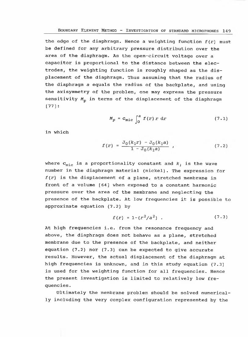
Bo u n d a r y E l e m e n t M ethod - In v e s t i g a t i o n of s t a n d a r d m i c r o p h o n e s 149

the edge of the diaphragm. Hence a weighting function f(r) must be defined for any arbitrary pressure distribution over the area of the diaphragm. As the open-circuit voltage over a capacitor is proportional to the distance between the elec­trodes, the weighting function is roughly shaped as the dis­placement of the diaphragm. Thus assuming that the radius of the diaphragm a equals the radius of the backplate, and using the axisymmetry of the problem, one may express the pressure sensitivity Mp in terms of the displacement of the diaphragm [77]:

Mp = Cmio Jo f(r)r dr (7.1)

in which

where cmic is a proportionality constant and k2 is the wave number in the diaphragm material (nickel). The expression for f(r) is the displacement of a plane, stretched membrane in front of a volume [64] when exposed to a constant harmonic pressure over the area of the membrane and neglecting the presence of the backplate. At low frequencies it is possible to approximate equation (7.2) by

f(r) = l-(r2/a2) . (7.3)

At high frequencies i.e. from the resonance frequency and above, the diaphragm does not behave as a plane, stretched membrane due to the presence of the backplate, and neither equation (7.2) nor (7.3) can be expected to give accurate results. However, the actual displacement of the diaphragm at high frequencies is unknown, and in this study equation (7.3) is used for the weighting function for all frequencies. Hence the present investigation is limited to relatively low fre­quencies.

Ultimately the membrane problem should be solved numerical­ly including the very complex configuration represented by the

150 T he Bo u n d a r y E l e m ent M eth od for So un d F ield Ca l c u l a t i o n s

backplate with holes. It would then be possible to express the sound field in terms of eigenfunctions of the membrane problem. Unfortunately, the geometry of this problem is very complex and may not be solved readily; furthermore the actual boundary condition at the edge of the diaphragm is unknown at this level of detail. In this line of thought the present investigation takes into account only the first order effect, by including the first term of the eigenfunction expansion, which is expected to be dominating by far at low frequencies.

When the microphone is exposed to a plane wave of zero degree incidence, the pressure is no longer constant over the area of the diaphragm but varies axisymmetric along the radius of the diaphragm. Defining its value relative to the undis­turbed incoming wave as p(r) allows one to establish an equa­tion for the free-field sensitivity;

Hence the sound field on the diaphragm is expanded into the eigenfunctions of the diaphragm problem (using only one term and neglecting all others), or explained in a more physical manner: the pressure acts through a certain weighting function.

Thus it is possible to derive an approximate expression for the free-field correction curve by combining equations (7.1) and (7.4);

Normally the free-field correction curve is given in a logar­ithmic scale: Fc = 2 0 log10/c.

If the angle of incidence differs from 0 or 180 degrees the pressure on the surface is no longer axisymmetric. In this case the incoming field should be dissolved in terms of eigenfunctions to the membrane problem including non-axisym­metric terms. However, due to the very careful crafting of the microphone and to the geometry of the volume between the diaphragm and the backplate, the diaphragm is very unlikely to

(7.4)

(7.5)

Bo u n d a r y E lem e n t M e th od - In v e s t i g a t i o n o f s t a n d a r d m i c r o p h o n e s 151

move non-axisymmetric, and even if a non-axisymmetric movement of the diaphragm could be provoked, the electrical output for each such mode would be zero due to cancelation. Hence only the axisymmetric part of the incoming wave contributes to the free- field correction curve. The axisymmetric part of the incident wave pI(P) is by equation (3.5):

Knowing the free-field correction curve for all angles of incidence makes it is possible to obtain an expression for the case of a microphone placed in a diffuse sound field:

7.2.2 MOVEMENT OF THE DIAPHRAGMIn order to increase the accuracy of the model, the move­

ment of the diaphragm must be taken into account. The movement of the diaphragm corresponds to a finite acoustic impedance of the microphone. From experimental results [71] the acoustic impedance is given in terms of the resonance frequency f0, the equivalent volume Veq and a loss factor d:

7 Ps•1 - _L}2 ♦ id-L

i»Veq f0j f0

where 7=1.4 is the ratio of specific heats and ps is the refer­ence static pressure (101.325 kPa). The movement of the dia­phragm could be taken into account by the means of a coupled structural-acoustic model, but in this study the coupled problem is decoupled at the interacting surface (the dia­phragm) , so that the structural and the acoustic problem may be handled separately. Defining the complex weighted pressure

the solution to the coupled problem may be found using an

(7.6)

(7.7)

JQa f (r) rdr(7.9)

152 T he Bo u n d a r y El e m e n t M e t h o d f o r So un d F ield Ca l c u l a t i o n s

iterative procedure: First the diaphragm is assumed to be blocked (volume velocity q0=0). This gives rise to a weighed pressure . Equation (7.8) then gives a first order approxi­

mation for the volume velocity g1=p^/Za. The correspondingdiaphragm velocity is vx (r) =2 (1-(r/a) 2) (wa2) , since themovement of the diaphragm is assumed to be parabolic. Then a combined radiation/scattering problem is solved to obtain a first order weighted pressure pj. This gives rise to a secondorder volume velocity, and so forth. The iteration is stopped when the difference between the modulus of two succeeding weighted pressures is sufficiently small (say, below 0*001 dB).

As another approximation for the movement of the diaphragm, scattering by a body shaped as a microphone may be considered, where the diaphragm is replaced with a locally reacting surface with the admittance:

S's = 2(l-(r/a)2)/Za/(*a2) . (7.10)

The two models would give the same result if the pressure was constant over the area of the diaphragm, since in this case the corresponding particle velocity on the surface would be para- bolically shaped as is the displacement of the diaphragm. Hence equation (7.10) is valid at low frequencies.

7.2.3 acoustic centreIn a reciprocity calibration arrangement the microphones

are used as receivers as well as sources. When the microphone is used as a source it is convenient to regard the microphone as a monopole. This simplification is valid at large distances from the microphone. However, the location of this equivalent monopole varies with the frequency, and is not exactly at the surface of the diaphragm. The location of the equivalent monopole for a given microphone and a given frequency is called the acoustic centre of the microphone. For the standard axial incidence arrangement the acoustic centre is located on the axis of the microphone, but for a general angle of observation

Bo u n d a r y El e m e n t M e t h o d - In v e s t i g a t i o n o f s t a n d a r d m i c r o p h o n e s 153

the acoustic centre will normally be located off-axis. The position of the acoustic centre is important for the determina­tion of the exact effective distance between the microphones in a reciprocity calibration arrangement, and for the B&K 4160 a standard table is provided [45-46]. Unless specified, the angle of observation is zero degrees (standard axial arrangement) in what follows.

7.3 RESULTSA number of calculations has been made on the B&K 4160 and

the 4180 condenser microphones. For the type 4160 microphone the protection grid was removed. In the free-field reciprocity calibration arrangement at the Acoustics Laboratory, the micro­phones are mounted on long rods, according to the requirements of reference [46], Hence the microphones can be assumed to be of semi-infinite shape. However, the BEM used here deals with finite bodies only, and hence the length of the microphones in the BEM code must be so large that the reflection from the end of the microphone is sufficiently small. For this purpose a length of 20 times the radius was found to be sufficient, whereas a length of 10 times the radius, which is approximately the length of a common preamplifier used with the microphones, was found to be too short. The microphones were then terminated with a hemisphere in the code. Figure 7.1 shows the geometry of the microphones as used in the code. All dimensions are in mm.

Since the standard condenser microphone B&K 4160 is more well-known through experiments than the B&K 4180, the results for the B&K 4160 are examined in details, whereas the results for the B&K 4180 are merely listed.

154 T he Bo u n d a r y E l e m ent M e t h o d f o r So un d F ield Ca l c u l a t i o n s

a) : b)

Figure 7-1. Simplified microphone geometry as used in the boundary element model. All dimensions are in mm. a) B&K 4160; b) B&K 4180

7.3.1 FREE-FIELD CORRECTION CURVESFor the B&K 4160 a series of three calculations was made.

For each calculation the mesh size was halved in order to examine the convergence of the method. In this way the calcula­tions were estimated to have converged to within 0*02 dB. The results shown are the ones determined with the finest mesh using 160 elements along the generator of the microphone model. Figure 7-2 shows the free-field correction curves obtained by measurements [71] and by calculation using the structural- acoustical model described in paragraph 7.2.2. The curve provided by Briiel and Kjaer [12] is also plotted, but it is hardly distinguishable from the measurements made at The Acoustics Laboratory in the scale of Figure 7-2. For the B&K 4160 an equivalent volume Veq = 150-10“9 m3, a loss factor d=l and a resonance frequency f0 = 8000 Hz were used in the model.

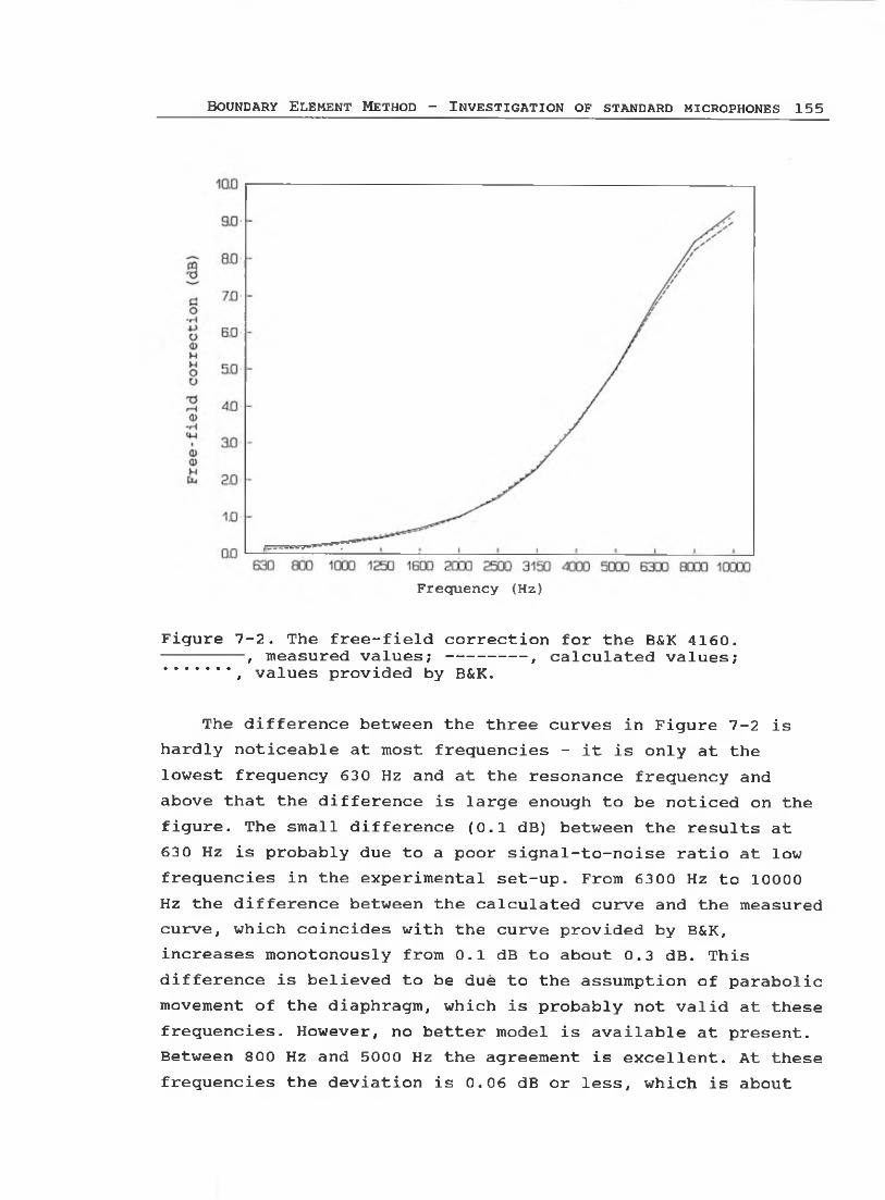
Bo u n d a r y E l e m e n t M e t h o d - In v e s t i g a t i o n of s t a n d a r d m i c r o p h o n e s 155

Frequency (Hz)

Figure 7-2. The free-field correction for the B&K 4160.-------- , measured values; -------- , calculated values;...... , values provided by B&K.

The difference between the three curves in Figure 7-2 is hardly noticeable at most frequencies - it is only at the lowest frequency 630 Hz and at the resonance frequency and above that the difference is large enough to be noticed on the figure. The small difference (0.1 dB) between the results at 630 Hz is probably due to a poor signal-to-noise ratio at low frequencies in the experimental set-up. From 6300 Hz to 10000 Hz the difference between the calculated curve and the measured curve, which coincides with the curve provided by B&K, increases monotonously from 0.1 dB to about 0.3 dB. This difference is believed to be due to the assumption of parabolic movement of the diaphragm, which is probably not valid at these frequencies. However, no better model is available at present. Between 800 Hz and 5000 Hz the agreement is excellent. At these frequencies the deviation is 0.06 dB or less, which is about

156 T he Bo u n d a r y E l e m ent M e t h o d f o r So un d F ield Ca l c u l a t i o n s

the total (numerical plus experimental) accuracy.In Figure 7-3 the ratio between the free-field correction

obtained with the structural-acoustical model and that obtained with a rigid model is shown. It can be seen that the movement of the diaphragm has no significance at the lowest frequencies as one would expect, since the acoustic impedance given by equation (7.8) increases towards infinity as the frequency goes towards zero. However, the effect increases with the frequency and is as large as 0.23 dB below the resonance frequency. As this effect is much larger than the deviation between the calculated and the measured free-field correction seen in Figure 7-2 it is concluded that the structural-acoustical model can be expected to give reliable results. The number of iter­ations used with this model was between 3 (for 630 Hz) and 7 (for 10000 Hz), and since each iteration makes use of the same factorization of A and therefore involves only an order of N2 flops, the time consumed by the iterations is negligible in comparison with the time used for the factorization of A, involving 2/3*W3 flops (for the 160 element model N=321).

F requen cy (Hz)

Figure 7-3. Influence of the finite impedance of the diaphragm of the B&K 4160. The curve is the ratio between the free-field corrections in dB obtained with the structural-acoustical model and with the rigid model.

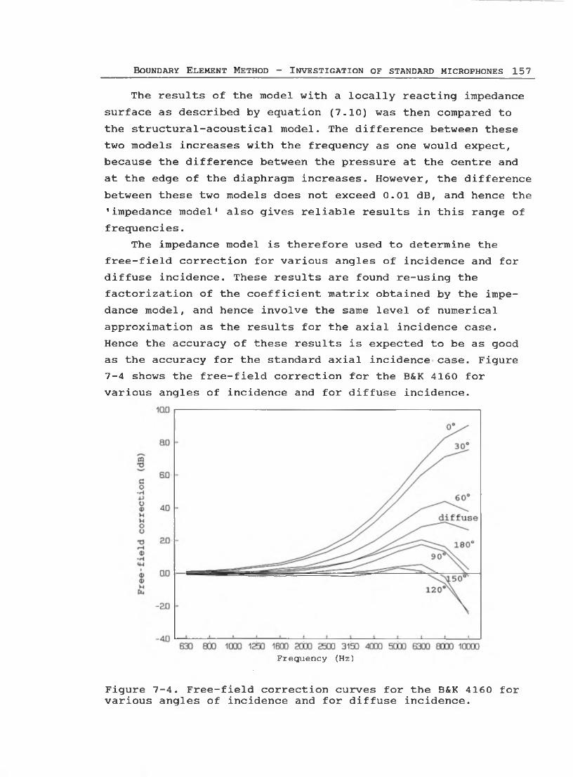
Bo u n d a r y E l e m e n t M e t h o d - In v e s t i g a t i o n o f s t a n d a r d m i c r o p h o n e s 157

The results of the model with a locally reacting impedance surface as described by equation (7.10) was then compared to the structural-acoustical model. The difference between these two models increases with the frequency as one would expect, because the difference between the pressure at the centre and at the edge of the diaphragm increases. However, the difference between these two models does not exceed 0.01 dB, and hence the 'impedance model' also gives reliable results in this range of frequencies.

The impedance model is therefore used to determine the free-field correction for various angles of incidence and for diffuse incidence. These results are found re-using the factorization of the coefficient matrix obtained by the impe­dance model, and hence involve the same level of numerical approximation as the results for the axial incidence case.Hence the accuracy of these results is expected to be as good as the accuracy for the standard axial incidence case. Figure 7-4 shows the free-field correction for the B&K 4160 for various angles of incidence and for diffuse incidence.

Frequency (Hz)

Figure 7-4. Free-field correction curves for the B&K 4160 for various angles of incidence and for diffuse incidence.

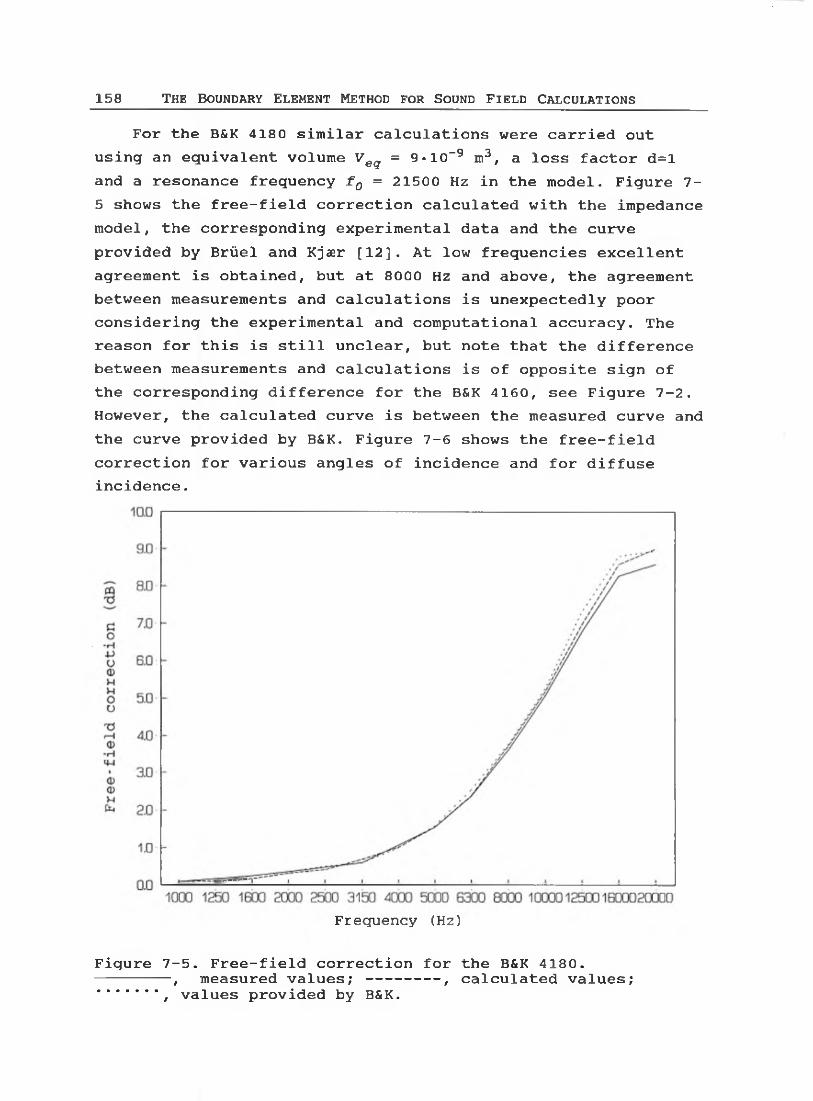
158 T he Bo u n d a r y E l em e n t M e t h o d for Soun d F ield Ca l c u l a t i o n s

For the B&K 4180 similar calculations were carried out using an equivalent volume Veq = 9*10"9 m3, a loss factor d=l and a resonance frequency f0 = 21500 Hz in the model. Figure 7- 5 shows the free-field correction calculated with the impedance model, the corresponding experimental data and the curve provided by Briiel and Kjaer [12]. At low frequencies excellent agreement is obtained, but at 8000 Hz and above, the agreement between measurements and calculations is unexpectedly poor considering the experimental and computational accuracy. The reason for this is still unclear, but note that the difference between measurements and calculations is of opposite sign of the corresponding difference for the B&K 4160, see Figure 7-2. However, the calculated curve is between the measured curve and the curve provided by B&K. Figure 7-6 shows the free-field correction for various angles of incidence and for diffuse incidence.

Frequency (Hz)

Figure 7-5. Free-field correction for the B&K 4180.-------- , measured values; -------- , calculated values;......., values provided by B&K.

Bo u n d a r y El e m e n t M eth od - In v e s t i g a t i o n o f s t a n d a r d m i c r o p h o n e s 159

10.0

8.0

§~ 6.0

-H4->© 4B uMOUTJ 2Di—io•H4-10) OB 0 w b

- 2.0

-4.0

Figure 7-6. Free-field correction curves for the B&K 4180 for various angles of incidence and for diffuse incidence.

7.3.2 acoustic centresIn the numerical model the acoustic centre was determined

by assuming a parabolic movement of the diaphragm. Having calculated the resulting pressure on the surface of the micro­phone, the calculation point P was moved outside the body in order to calculate the on-axis pressure at various distances from the diaphragm. In the far-field the pressure follows the 1/r-law, where r is the distance to the diaphragm minus the value of the acoustic centre, r = dd±a-dac. Note that the acoustic centre is defined to be positive outside the micro­phone. Hence the product of the magnitude of the calculated pressure and the effective distance r should remain constant in the far-field, and the estimate of the acoustic centre is adjusted until this condition is met. Figure 7-7 shows the calculated deviations from the 1/r-law on-axis for two fre-

Frequency (Hz)

160 T h e Bo u n d a r y E l e m e n t M eth od for So u n d F ield Ca l c u l a t i o n s

quencies for the B&K 4160 microphone versus the distance to the diaphragm. The effect of altering the estimate of the acoustic centre by 0.5 mm is also shown, and the figure indicates an uncertainty of about 0.2 mm on the value of the acoustic centre.

Distance to diaphragm (mm)

Figure 7-7. Calculated deviations from the 1/r-law for the B&K4160. -------- , 630 H z ? --------- 10000 Hz. The two centralcurves correspond to the final estimate of the acoustic centre. The two upper and the two lower curves correspond to alter­ations of +0.5 mm of the estimate of the acoustic centre.

Figure 7-7 suggests that at both frequencies the near-field extends to about 200 mm, and this is also the case for the fre­quencies in between. The extent of the near-field is important for the experimental set-up: The microphones should be placed in the far-field but as close as possible in order to maintain an acceptable signal-to-noise ratio at low frequencies.

Figure 7-8 shows the acoustic centres for the B&K 4160 microphone versus frequency. The calculated values are shown together with the measured value and the values stated in IEC publication 486 [45].

Bo u n d a r y E l e m e n t M eth od - In v e s t i g a t i o n o f s t a n d a r d m i c r o p h o n e s 161

Frequency (Hz)

Figure 7-8. Acoustic centre for the B&K 4160. -------- ,measured; ........ , IEC 486; , calculated estimate.

Due to reflections from the end of the microphone model in the code, the calculated values oscillate around a smooth dependence of frequency. The figure shows a good agreement between the calculated and the measured values up to about 6300 Hz. The deviation from 6300 Hz and above is believed to be due to the assumption of parabolic movement of the diaphragm, which is probably not valid at high frequencies. However, the agree­ment with the values stated in IEC Publication 486 [45] is good.

In Figure 7-9 the calculated acoustic centres for the B&K 4180 are shown together v/ith the measured data. Such values has not yet been published for the B&K 4180. The agreement between the calculated and measured values is acceptable at low fre­quencies when the experimental uncertainty is taken into account: a change of 1 mm in the position of the acoustic

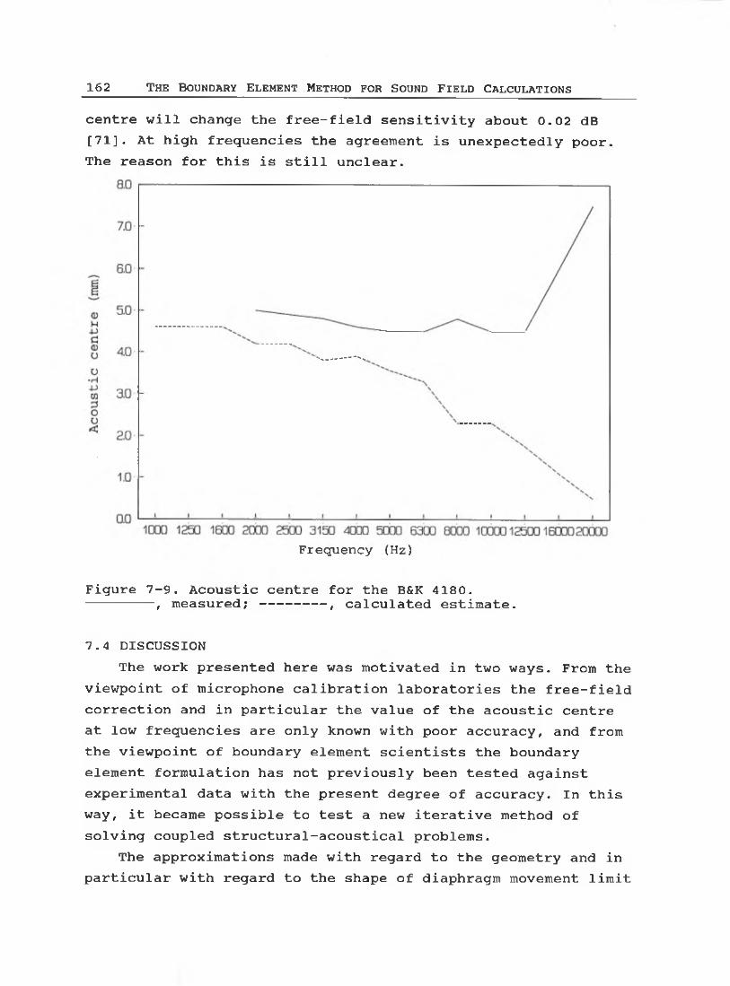
162 T he Bo u n d a r y E l e m e n t M eth od f o r Soun d F ield C a l c u l a t i o n s

centre will change the free-field sensitivity about 0.02 dB[71]. At high frequencies the agreement is unexpectedly poor. The reason for this is still unclear.

Frequency (Hz)

Figure 7-9. Acoustic centre for the B&K 4180.-------- , measured;--------, calculated estimate.

7.4 DISCUSSIONThe work presented here was motivated in two ways. From the

viewpoint of microphone calibration laboratories the free-field correction and in particular the value of the acoustic centre at low frequencies are only known with poor accuracy, and from the viewpoint of boundary element scientists the boundary element formulation has not previously been tested against experimental data v/ith the present degree of accuracy. In this way, it became possible to test a new iterative method of solving coupled structural-acoustical problems.

The approximations made with regard to the geometry and in particular with regard to the shape of diaphragm movement limit

Bo u n d a r y E le m e n t M eth od - In v e s t i g a t i o n o f s t a n d a r d m i c r o p h o n e s 163

the model to frequencies below the first resonance of the diaphragm. At these frequencies the calculated data are in excellent agreement with the measured data. A better knowledge of the diaphragm movement would be required for improving the results at higher frequencies. All frequencies considered in this study are below the undesirable 'characteristic frequen­cies' discussed in chapter 5, and hence no special care had to be taken of this phenomenon.

Structural-acoustical coupling is in particular of interest in problems where the coupling is strong, e.g. scattering and radiation by structures submerged in water [6]. Usually such calculations are accomplished by using finite element calcula­tions for the structure and boundary element calculations for the fluid. Normally these calculations are carried out by combining the boundary element equations with the finite element matrix. Hence the elements of the finite element matrix corresponding to the nodes on the interacting surface are changed. However, this approach may give rise to some problems: The very large systems of equations of the finite element method may only be solved effectively if the coefficient matrices are bandlimited and symmetric, but unfortunately the equations from the boundary element method are unsymmetric and may increase the 'bandwidth' of the finite element matrices. Furthermore, it is often desirable to operate with different mesh-sizes for the structural model and for the boundary element model, since the wavelength normally differs in the two domains [67]. The iterative method described in this study may readily be used for different mesh-sizes as well as for differ­ent interpolation functions, whereas special care must be taken to handle such cases with the standard approach. Finally, for cases where the number of nodes of the interacting surface is small compared to the number of nodes in both the finite element and the boundary element models, the iterative method might be faster than the standard approach, since the factorization of the two matrices from the respective methods will be 'cheaper' in terms of flops than the factorization of the larger combined matrix, due to the N3 behaviour of matrix

164 T h e Bo u n d a r y E l e m e n t M eth od f o r s o u n d F ield Ca l c u l a t i o n s

factorization. Note that when taking the bandlimited structure of the finite element matrix into account a more complex formula for the number of flops required arises, but the general trend of flops versus matrix size remains.

7.5 CONCLUDING REMARKSIn this chapter the free-field correction curve for stan­

dard condenser microphones has been calculated by means of the boundary element method. Due to approximations made in the modelling the microphones this investigation is limited to frequencies below the first resonance of the diaphragm. In this range of frequencies the calculated results agree excellently with measured data. The free-field correction curve for various angles of incidence and for diffuse incidence has been calcu­lated as well. For calibration laboratories various secondary characteristics associated with the microphones are important. These quantities are extremely difficult to determine experi­mentally and the calculation of these may therefore prove to be valuable for calibration laboratories and microphone designers.

In order to achieve the desired high precision, the move­ment of the diaphragm had to be taken into account. Hence a coupled structural-acoustical problem was considered. In this study a new iterative method of solving coupled structural- acoustic problems has been presented. This method allows the coupled problem to be separated at the surface of interacting, so that the structural and the acoustic problem may be treated separately. The benefits of this method are its simplicity and its flexibility with respect to the handling of problems where different numerical methods, mesh-sizes and interpolation functions are used in the two domains. A paper describing this work has been accepted for publication [53].

Bo u n d a r y E l e m e n t M e t h o d - S p e c t r a l St e r e o T heory 165

8. APPLICATION OF THE B O U N D A R Y ELEMENT

M E T H O D TO SPECTRAL STEREO THEORY

In a collaborative work with associate professor Karsten Bo Rasmussen the axisymmetric integral equation formulation was used to calculate the diffraction caused by a body with a shape that to some extent resembles the human head. The diffraction caused by the head of a listener is important for determining the relation between the loudspeaker signals in a spectral stereo setup. This work resulted in a paper, which has been published in Journal of the Audio Engineering Society [72]. In this chapter the work will be shortly motivated and the bound­ary element calculations will be presented. Finally, the con­clusions of the joint work will be outlined. The paper in its full length is included as appendix A of this thesis.

8.1 MOTIVATIONCooper and Bauck have established an elaborate model for

the relationship between stereo loudspeaker signals and an equivalent phantom source [23-26]. They have developed math­ematical expressions for the determination of loudspeaker signals, which should be able to produce any specified phantom source in the mind of the listener.

The approach is that when superimposed at the ears, loud­speaker signals should closely resemble a plane wave coming from a well defined horizontal direction - the so-called phantom direction. When this assumption is met, the loudspeaker signals will supposedly provide the listener with a clear and unambiguous sense of direction of the sound. Free field condi­tions are assumed in the sense that the listening room is nottaken into account. This may be justified by means of the Haaseffect or the law of the first wavefront [7] stating that thefirst part of the sound field is very important for localiz­ation.

Thus a plane wave represent the direction of the phantom source - the direction which should be simulated by the loud­speaker signals. Hence, the loudspeaker signals should be

166 T he Bo u n d a r y E lem e n t M e th od for So un d F ield Ca l c u l a t i o n s

adjusted so that the total sound field from both speakers at the ear positions of the artificial head is identical to the sound field due to a plane incoming wave from the phantom direction. In order to obtain the relation between the loud­speaker signals, which lead to any particular phantom direc­tion, the diffraction caused by the listener must be taken into account.

Cooper and Bauck have treated the situation as ideal in the sense that room reflections have not been taken into account and that the head was regarded as being spherical. It is the latter assumption regarding the head shape that is investigated further in this study. Obviously the shape of a human head is not spherical, but this simple approximation becomes plausible when combined with ear locations shifted tov/ards the back of the head rather than placed along a diameter. It is of import­ance to determine the validity of this simple approximation. Ultimately one could wish to make accurate calculations on a dummy head including the effect of the pinna and the torso, but doing this would still with modern computing be quite a time and storage consuming task. In order to be able to solve the problem on a normal PC the improved head shape has been chosen to be axisymmetric so that the axisymmetric integral equation formulation developed in chapter 3 may be used. This is obvi­ously not yet an accurate model of the shape of the human head. However, it becomes possible to take into account the fact that the head is higher than it is wide (frontal view) without any loss of generality as far as the location of the ears is concerned. Since horizontal localisation is to be investigated, the generator of the axisymmetric shape is chosen to be a horizontal section of the Briiel & Kjasr 4128 Head-And-Torso- Simulator (HATS) passing through the ear positions as sketched in Figure 8-1. The improved head shape was assumed to be rigid.

Bo u n d a r y E l e m e n t M e t h o d - S p e c t r a l S t e r e o T heo ry 167

Front up

Figure 8-1. Cross sections through the centre of improved head model. The horizontal cross section is that of the Briiel & Kjaer 4128 head-and-torso simulator passing through the ear posi­tions. The positions of the ears are indicated by arrows. All measures are in millimetres. The model is symmetrical around horizontal axis through the centre.

8.2 CALCULATION OF THE DIFFRACTION CAUSED BY THE IMPROVEDHEAD SHAPE.Calculations were made using the axisymmetric integral

equation formulation described in chapter 3. Isoparametric linear elements were used to discretize the generator of the improved head shape shown in Figure 8-1. Calculations were carried out in the frequency range 100Hz - 6400Hz. In the frequency range 100Hz - 2000Hz 37 elements were used to model the generator, whereas 75 elements were used in the frequency range 2000Hz- 6400Hz. For all frequencies it was found that four terms of the cosine expansion of equation (3.38) sufficed for an accurate calculation. Figure 8-2 shows the pressure at the left ear of the improved head shape relative to the pres­sure of thje undisturbed plane wave as a function of the frequency and the angle of incidence as defined in the inset in the figure.

168 T h e Bo u n d a r y El e m e n t M e t h o d for Sou n d F ield Ca l c u l a t i o n s

Frequency (Hz)

Figure 8-2. Relative magnitude of the pressure at the left ear of the improved head shape when scattering of a plane wave is considered. The relative magnitude of the pressure is shown as a function of the frequency and of the angle of incidence as defined in the small inset in the figure.

Bo u n d a r y Ele m e n t M e t h o d - S p e c t r a l S t e r e o T heo ry 169

8.3 CONCLUDING REMARKSIn the paper included in appendix A the results obtained

with the improved head shape were then compared to the results obtained with the original spherical head shape. It was found that since the angles of incidence used for an ideal stereo setup are close to frontal incidence e.g. -30°<a<300, the spherical head shape assumption produces results of sufficient accuracy. However, it was found that the diameter of 175 mm of the equivalent sphere commonly used was too large, whereas a diameter of 137 mm appeared to be more appropriate.

170 T h e Bo u n d a r y E l e m e n t M e t h o d f o r So u n d F ield Ca l c u l a t i o n s

9. D ISC U SS IO N

The present study has mainly been discussed current with the development of the text in the partial conclusions. How­ever, the author thinks that a few ideas for further work deserves to be emphasized in this chapter. Hence, in this chapter a few suggestions for further work will be given. Section 9.1 deals with the topic of convergence, which was introduced in section 4.6, and section 9.2 outlines some problems for which the QR factorization may advantagously be used.

9.1 DISCUSSION OF CONVERGENCEThe topic of convergence was introduced in section 4.6, and

a few test cases were studied. However, the situation turned out to be far more complicated than it was the case with convergence of numerical integration formulas, as discussed in section 4.6. In the following some remarks to a further inves­tigation of convergence of boudary elements formulations are given.

The error made by a boundary element formulation may be divided into two parts. The first part is the initial error, which is the error due to a given discretization, say, two elements per wavelength. If this initial error is altered it corresponds to a vertical displacement of the curves shown in figures 4-17, 4-19, 4-20, 4-21, and 4-24. The second part is associated with the convergence rate of the methods i.e. the rate by which the error decreases when the mesh is refined.This part corresponds to the slope of the curves mentioned above. The desirable behavior of a boundary element implementa­tion is to possess both a small initial error and a high rate of convergence. In the study of numerical integration it was found that a high order formula generally produces both a smaller initial error and a higher rate of convergence than a low order formula. Although the situation is much less clear when studying the error made by boundary element formulations, this conclusion generally holds for the formulations considered in section 4.6 as well. In section 4.6 convergence was investi-

Bo u n d a r y El e m e n t M eth od - D i sc ussi on 171

gated at a relatively low frequency, ka=1, where a was a typical dimension of the body. At higher frequencies the non­uniqueness problem must be taken into account when examining the convergence, since the error made by the boundary element model increases when there is a characteristic frequency in the neighbourhood of the frequency of interest. Although the accuracy of different methods to overcome the non-uniqueness problem has been adressed in the literature [42,84] no system­atic investigation of the convergence of different formulations used to overcome the non-uniqueness problem discussed in chapter 5 has been reported. The author believes that a study of the convergence of the different boundary element formula­tions would be very valuable at this stage. Such a study should involve higher frequencies, as well as bodies of more complex shapes, such as thin bodies and bodies with sharp edges.

9.2 FURTHER APPLICATIONS OF THE QR FACTORIZATIONThe QR factorization is a relatively unknown factorization

method for scientists that are working outside the area of numerical linear algebra. Moreover, since the RRQR factorization is a very recent development of the standard QR factorizations, the knownledge of this factorization is even less widespread. However, the QR factorization is almost as efficient as the well-known LU factorization, more stable for solving large systems of equations [39], and more efficient in solving overdetermined systems of equations. Furthermore, the ease with which the QR factorization may be updated when a row or a column of the boundary element coefficient matrix is appended or deleted may be used advantagously in boundary element calculations, as will be described in paragraph 9.2.1. The rank revealing QR factorization may for some applications be used as an alternative to the singular value decomposition, as will be described in paragraph 9.2.2.

9.2.1 UPDATING THE QR FACTORIZATIONIn the beginning of section 4.6 it was mentioned that

elements of equal size would seldom be the optimal choice with

172 T he Bo u n d a r y E le m e n t M eth od f o r Sou n d F ield Ca l c u l a t i o n s

respect to accuracy vs. calculation time for practical boundary element calculations. It was stated that small elements should be used where the geometry or the acoustic variables vary quickly. However, since the variation of the unknown acoustic variable is not known initially, the optimale sizing of the elements is rarely known in advance. In this connexion the ability of the QR factorization to be updated may prove valu­able.

Consider for simplicity a constant element implementation of a boundary element formulation. Now, if a given problem has been calculated using a coarse discretization it might be required to refine the mesh locally, where a quick variation of e.g. the pressure is observed. In the boundary element coeffi­cient matrix the refinement of an element corresponds to deleting the row and the column which correspond to that element, and then adding a number of rows and columns corre­sponding to the new elements. If the number of elements that are refined is small compared to the total number of elements, an updating of the QR factorization may advantagously be carried out instead of calculating a new factorization from scratch. Note that the same technique may be used if the position of a small number of elements is altered, which is the case when making slight changes to the geometry. Slight changes to the geometry is often made in a design process. For higher order elements the general idea is the same - although an element corresponds to several rows and columns in the coeffi­cient matrix in this case.

Updating the QR factorization may also be advantagous when new equations are added to the orginal system of equations by the CHIEF method or a related approach as mentioned in the end of section 6.3.

9.2.2 USING THE RANK REVEALING QR FACTORIZATION AS AN ALTERNATIVE TO THE SINGULAR VALUE DECOMPOSITION

In a recent paper by Bai [3], the singular value decomposi­tion was used to find the eigenfrequencies and eigenmodes of an enclosure. It was demonstrated that an eigenfrequency could be

Bo u n d a r y E lem e n t M e th od - D i sc ussi on 173

detected by examining the smallest singular value, which becomes small near an eigenfrequency. For the case of multiple eigenfrequencies a number of singular values corresponding to the multiplicity of the eigenfrequency become small. The corresponding singular vectors contains the eigenmode(s) corresponding to the eigenfrequency [3]. In this case the RRQR factorization could provide the same information as the singu­lar value decomposition much cheaper in terms of computational time. Since the boundary element method operates in the fre­quency domain the eigenfrequencies was found by generating the boundary element coefficient matrix in a frequency range using a coarse resolution (3). The estimate of an eigenfrequency was then improved by a so-called golden search algorithm [3]. Recently a frequency interpolation technique has been described [6,90], by which the sound field within an enclosure was obtained approximately in a range of frequencies by means of an interpolation scheme using a small number of key frequenicies, and very recently Wu et al. [110] has proposed a so-called 'Green's function interpolation technique' for speeding-up multi-frequency run. These interpolation schemes might advan­tagously be used instead of the much more time consuming initial frequency sweep used by Bai [3].

174 T he Bo u n d a r y El e m e n t M e t h o d for Soun d F ield Ca l c u l a t i o n s

10. C O N C L U S IO N S

In this study a boundary element method based on Helmholtz integral equation has been considered. During the work computer programs have been developed for calculating the sound field exterior to bodies of axisymmetric or general three-dimensional shape, positioned in free space. The study involved the follow­ing partial accomplishments.

In chapter 2 some fundamental concepts were presented. Helmholtz integral equation was derived mathematically, and a more intuitive physical explanation was given following that of Baker and Copson [4].

In chapter 3 an axisymmetric integral equation formulation for non-axisymmetric boundary conditions was developed. Non- axisymmetric boundary conditions were handled by expanding the sound field in a circumferential cosine series. In relation to the existing literature [2,82] this work presents a novel way of handling the singularities in the resulting integrals of the expansion by means of elliptic integrals, as suggested for the fully axisymmetric case in reference [82]. However, as this work was submitted for publication [51] it turned out that similar work had been carried out simultaneously by other researchers [55,93].

Chapter 4 concerns the numerical implementation of the boundary element formulations. The benefit of using high order shape functions adopted from the finite element method by Seybert and his co-workers, was intuitively justified by observing the convergence of various numerical integration formulas. A brief investigation of the convergence properties of three implementations of the axisymmetric integral equation formulation, using different shape functions, was then carried out. For the case of scattering by a rigid cylinder it was shown that a new generalized quarter-point technique could improve the accuracy. In this chapter a superparametric imple­mentation of both the axisymmetric and the three-dimensional formulations was proposed. Superparametric elements has not previously been used for acoustic boundary element calcula­tions, as far as the author knows.

Bo u n d a r y E lem e n t M e t h o d - Co n c l u s i o n s 175

Chapter 5 concerns the non-uniqueness problem. The term non-uniqueness problem refers to the fact that the surface Helmholtz integral equation is unable to obtain a unique sol­ution at certain characteristic frequencies. One of the methods- the Combined Helmholtz Integral Equation Formulation (CHIEF)- proposed in the literature for partially circumventing the non-uniqueness problem was studied in detail, and a short survey of other methods proposed in the literature was given. Furthermore, this chapter contains a new explanation of the non-uniqueness problem by means of an analogy to active sound control.

Chapter 6 addresses the problem of solving a set of linear equations. It was demonstrated that the non-uniqueness problem appears as a numerical rank deficiency of the boundary element coefficient matrix. In chapter 6 the use of rank revealing factorizations of the boundary element coefficient matrix, with the CHIEF method or related methods, was then proposed. The combination of the CHIEF method and a rank revealing factorization efficiently ensures a unique solution at charac­teristic frequencies. The use of rank revealing factorizations in this connexion has not previously been reported, as far as the author knows. For the solution of the system of equations produced by the boundary element method, the author highly recommends the QR factorization, as described in section 6.3. This is due to the rank revealing properties of the RRQR factorization, the efficiency and stability of this factorization when solving overdetermined systems of equations, and the ability of this factorization to be updated efficient­ly, which is of great importance when adding CHIEF points or making slight changes to the geometry, as discussed in chapter 9.

In chapter 7 the boundary element method was used to calculate the pressure sensitivity correction curves for two standard microphones. The boundary element calculations were tested against very accurate experimental results, allowing the axisymmetric formulation to be verified for more complicated shapes than the sphere extensively used throughout the study.

176 T he Bo u n d a r y E le m e n t M eth od for Soun d F ield Ca l c u l a t i o n s

In this chapter the coupled structural-acoustic problem of the diaphragm of the microphone and the surrounding air was solved by means of an iterative process. Even though this iterative process is straightforward and therefore supposedly has been used by other researchers the author is not aware of any description of this approach in the literature.

Chapter 8 describes a final application of the axisymmetric formulation to spectral stereo theory, where the assumption of spherical head shape was tested against a more realistic head shape. It appeared that the common assumption of spherical head shape is reasonable for angles of incidence close to frontal incidence, but that a smaller diameter of the sphere than usually used, should be preferred.

Finally, chapter 9 contains a discussion of the work with some suggestions for further work.

Bo u n d a r y E lem e n t M e t h o d - Re f e r e n c e s 177

REFERENCES

The references are listed alphabetically. A recent list of State-of-the-Art references has recently been given inBoundary Element Methods in Acoustics (R.D. Ciskowski and C.A. Brebbia, editors). Appendix State-of-the-Art References in Boundary Element Applications to Acoustics. Computational Mechanics Publications Co-published with Elsevier Applied Science.1. A bramowitz M. , and Stegun I.A. 1965

Handbook of Mathematical Functions. National Bureau of Standards.

2. AKYOL T.P. 198 6Acustica 61, 200-212. Schallabstrahlung von Rota- tionskorpern. (In German).

3. Bai M.R. 1992Journal of the Acoustical Society of America 91, 2529-2538. Study of acoustic resonance in enclo­sures using eigenanalysis based on boundary element methods.

4. Baker B.B. and Copson E.T. 1953The Mathematical Theory of Huygens' Principle.Second Edition Oxford University Press.

5. Banaugh R.P., and Goldsmith W. 1963Journal of the Acoustical Society of America 35, 1590-1601. Diffraction of Steady Acoustic waves by Surfaces of Arbitrary shape.

6. Benthien G.w. and Schenck H.A. 1991in Boundary Element Methods in Acoustics (R.D. Ciskowski and C.A. Brebbia, editors). Chapter 6. Structural-Acoustic Coupling. Computational Mecha­nics Publications Co-published with Elsevier Appli­ed Science.

7. Blauert J. 1983Spartial Hearing. M.I.T.Press, Cambridge, Mass.

8. Brebbia C.A., Telles J.C.F., and W robel L.C. 1984Boundary Element techniques. New York: Springer.

9. Br e b b i a C.A., and W a l k e r S. 1980Boundary Element techniques in engineering. Newnes - Butterworths London.

178 T he b o u n d a r y El e m e n t M e t h o d f o r Soun d F ield Ca l c u l a t i o n s

10 .

1 1 .

12.

13.

14 .

15.

16.

17.

18.

19.

20.

BROD K. 1984Journal of the Acoustical Society of America 76, 1238-1243. On the uniqueness of solution for all wavenumbers in acoustic radiation.

Bruel P.V. and Rasmussen G. 1959Briiel & Kjaer, Technical Review no.2. Free-field responce of condenser microphones (Part II).

Bruel & Kjsr 1986Instruction Manual. Condenser Microphones One-Inch Type 4160 and Half-Inch Type 4180

Burton A.J., and Miller G.F. 1971Proceedings of the Royal Society of London A323, 201-210. The application of integral equation met­hods to the numerical solutions of some exterior boundary value problems.

Busk T. 1977Polyteknisk forlag/Special-Trykkeriet a-s Viborg. Numerisk integration (Numerical Integration). (In Danish).

Byrd P.F., and Friedman M.D. 1971Handbook of Elliptic Integrals for Engineers and Scientists. New York: Springer.

Chan t .f . 1987Linear Algebra and its Applications 88/89, 67-82. Rank revealing QR factorizations.

Chen L.H., and Schweikert 1963Journal of the Acoustical Society of America 35, 1626-1632. Sound radiation from an Arbitrary Body.

Cheng C.Y.R., Seybert A.F. 1987SAE 1987 Noise and Vibration Conference. Recent applications of the Boundary Element Method to Problems in Acoustics.

Cheng C.Y.R., Seybert A.F., and Wu T.W. 1991Journal of Sound and Vibration 151, 119-129. A multi domain boundary element solution for silencer and muffler performance prediction.

Chertock G., 1964Journal of the Acoustical Society of America 36, 1305-1313. Sound Radiation from Vibrating Surfaces.

Chertock G. , 1969Journal of the Acoustical Society of America 47, 387-388. Solutions for Sound-Radiation Problems by Integral Equations at the Critical Wavenumbers.

Bo u n d a r y E lem e n t M e th od - R ef e r e n c e s 179

22 .

23 .

24.

25.

26.

27.

28.

29.

30.

31.

32.

Chien C.C., Rajiyah H., and Atluri S.N. 1990Journal of the Acoustical Society of America 88, 918-937. An effective method for solving the hyper­singular integral equations in 3-D acoustics.

Cooper D.H. 1982Journal Audio Engineering Society 30, 34-38. Cal­culator program for Head-Related Transfer Function.

Cooper D.H. 1983Journal Audio Engineering Society 31, 760. Phase Reference in HRTF calculation.

Cooper D.H. 1987Journal Audio Engineering Society 35, 629-642. Problems with Shadowless Stereo Theory.

Cooper D.H., and Bauck J.L. 1987Journal Audio Engineering Society 37, 3-19. Pro­spects for Transaural Recording.

Copley L.G. 1967Journal of the Acoustical Society of America 41, 807-816. Integral Equation Method for Radiation from Vibrating Bodies.

Copley L.G. 1968Journal of the Acoustical Society of America 44, 28-32. Fundamental results concerning integral representations in acoustic radiation.

Cristescu M. , and Loubignac G. 1978in Recent Advances in Boundary Element Methods (C.A. Brebbia, editor). Gaussian Quadrature For­mulas for Functions with Singularities in 1/R over Triangles and Quadrangles. Pentech Press, London.

Cunefare K.A. , Koopmann G.,and Brod K. 1989Journal of the Acoustical Society of America 85,39-48. A boundary element method for acoustic radi­ation valid for all wavenumbers.

Cunefare K.A. , Koopmann G.H. 1992Journal of Vibration and Acoustics - Transactions of the ASME 114, 178-186. Acoustic Design Sensiti­vity for Structural Radiators.

Dankert J. 1977Numerische Methoden der Mechanik 202-206. Springer- Verlag Wien New York. (In German)

Dongarra J.J. et al. 1979LINPACK User's Guide Philadelphia: Society for Industrial and Applied Mathematics.

180 T he Bo u n d a r y E l e m e n t M eth od f o r Sou n d F ield Ca l c u l a t i o n s

34.

35.

36.

37.

38.

39.

40.

41.

42.

43 .

DOKUMACI E. 1990Journal of Sound and Vibration 139, 83-97. A study of the failure of numerical solutions in boundary element analysis of acoustic radiation problems.

Engblom J.J., and Nelson R.B. 1975Journal of Applied Mechanics - Transactions of the ASME, ASME paper no. 75-AMPW-54, 295-300. Consist­ent Formulation of Sound Radiation From Arbitrary Structure.

Francis D.T.I. 1991Journal of Sound and Vibration 145, 495-498. Parti­al use of the Helmholtz Gradient Formulation to obtain unique solutions to acoustic radiation pro­blems at characteristic frequencies.

Francis D.T.I 1993Journal of the Acoustical Society of America 93, 1700-1709. A gradient formulation of the Helmholtz integral equation for acoustic radiation and scat­tering.

Fyfe K.R., and Ismail F. 1989Journal of Sound and Vibration 128, 361-376. An investigation of the acoustic properties of vibra­ting finite cylinders.

Golub G.H.,and Van Loan C.F. 1989Matrix Computations, 92-104. The John Hopkins Uni­versity Press, 2nd Edition.

Gradshteyn I.S., and Ryzhik I.M. 1965Table of Integrals, Series, and Products. New York and London: Academic Press.

Hahn S.R., Ferri A.A., and Ginsberg J.H. 1991in Structural Acoustics (R.F.Keltie, A.F.Seybert,D.S.Kang, L.Olson and P.Pinsky, editors), NCA- Vol.12/AMD-Vol.128, ASME, New York, 223-234. A review and evaluation of methods to alleviate non­uniqueness in the surface Helmholtz integral equa­tion.

Hall W.S., and Robertson W.H. 1988Journal of Sound and Vibration 126, 367-368. Stan­dard Helmholtz integral equation calculations near characteristic frequencies.

Hwang J.-Y., and Chang S.-C. 1991Journal of the Acoustical Society of America 90, 1167-1180. A retracted boundary integral equation for exterior acoustic problem with unique solution for all wavenumbers.

Bo u n d a r y E le m e n t M eth od - R e f e r e n c e s 181

44.

45.

46.

47.

48 .

49.

50.

51.

52 .

53.

Henwood D.J. 1993Journal Audio Engineering Society 41, 485-496. The Boundary-Element Method and Horn Design.

IEC Publication 486 1974Precision method for free-field of one-inch stan­dard condenser microphones by the reciprocity tech­nique,

IEC Publication 1094-3: WG-draft 1992Measurement microphones, Part 2: Primary method for free-field calibration of laboratory standard mi­crophones by the reciprocity technique.

J eans R, and Mathews I.e. 1992Journal of the Acoustical Society of America 92, 1156-1166. The wave superposition method as a ro­bust technique for computing acoustic fields.

Jones D.S. 1974Quarterly Journal of Mechanics and Applied Mathema­tics 27, 129-142. Integral Equations for the ex­terior acoustic problem.

JUHL P.M. 1991Report no. 47, The Acoustics Laboratory, Technical University of Denmark. Axisymmetric integral for­mulation for non-axisymmetric boundary conditions.

J UHL P.M. 1992Proceedings. Second International Congress on Re­cent Developments in Air. and Structure-Borne Sound and Vibration 965-972. On selecting CHIEF to over­come the nonuniqueness problem in boundary element methods.

JUHL P.M. 1993Journal of Sound and Vibration 163, 397-406. An axisymmetric integral equation formulation for free space non-axisymmetric radiation and scattering of a known incident wave.

JUHL P.M. 1994 (?)To appear in Journal of Sound and Vibration. A numerical study of the coefficient matrix of the boundary element method near characteristic frequ­encies .

J uhl P.M. 1994 (?)To appear in Journal of Sound and Vibration. A numerical investigation of standard condenser mi­crophones.

182 T he Bo u n d a r y Ele m e n t M eth od for Sou n d F ield Ca l c u l a t i o n s

54.

55.

56.

57.

58.

59.

60.

61.

62.

63.

64 .

65.

Kawai Y., and T erai T. 1990Applied Acoustics. The Application of Integral Equation Methods to the Calculation of Sound Atte­nuation by Barriers.

K im H .S . , K im J.S., and Kang H.J. 1993Journal of Sound and Vibration 163, 385-396. Acous­tic wave scattering from axisymmetric bodies.

K leinmann R.E., Roach G.F., Schuetz L.S., and Shirron J.1988

Journal of the Acoustical Society of America 84, 385-391. An iterative solution to acoustic scat­tering by rigid objects.

Koopmann G.H., Song L. , and Fahnline J.B. 1989Journal of the Acoustical Society of America 86, 2433-2438. A method for computing acoustic fields based on the principle of wave superposition.

Lamb H. 1932hydrodynamics Sixth Edition. New York Dover Publications 1945.

Malbequi P., Candel S.M., and R ignot E. 1987Journal of the Acoustical Society of America 82,1771-1781. Boundary integral calculations of scat­tered fields: Application to a spacecraft launcher.

Martinez R. 1991Journal of the Acoustical Society of America 90,2728-2738. The thin-shape breakdown (TSB) of theHelmholtz integral equation.

Mathews I.e. 1986Journal of the Acoustical Society of America 79, 1317-1325. Numerical techniques for three-dimensio­nal steady-state fluid-structure interaction.

Meyer W.L., Bell W.A. , Zinn B.T. , and Stallybrass M.P. 1978 Journal of Sound and Vibration 59, 245-262. Boun­dary integral solutions of three dimensional acoustic radiation problems.

M eyer W.L. , Bell W.A., Stallybrass M.P., and Z inn B.T. 1979 Journal of the Acoustical Society of America 65, 631-638. Prediction of the sound field radiated from axisymmetric surfaces.

MORSE P.M. 1948Vibration and Sound. McGraw-Hill; (second edition).

Morse P.M., and Ingard K.U. 1986Theoretical Acoustics. New York: McGraw-Hill.

Bo u n d a r y E lem e n t M e t h o d - R e f e r e n c e s 183

6 6.

67.

68.

69.

70.

71.

72.

73.

74.

75.

76.

OCHMANN M. 1990Acustica 72, 233-246. Die Multipolstrahlersynthese - ein effektives Verfahren zur Berechnung der Schallabstrahlung von schwingenden Strukturen be- liebiger Oberflachengestalt. (In German)

OCHMANN M. , and Wellner F. 1991Acustica 73, 177-190. Berechnung der Schallabstrah­lung dreidimensionaler schwingender Korper mit Hilfe eines Ranselemente-Mehrgitterverfahrens. (In German)

Piaszczyk C.M. , and Klosner J.M. 1984Journal of the Acoustical Society of America 75, 363-375. Acoustic radiation from vibrating surfaces at characteristic frequencies.

Pierce a .d . 1981Acoustics: An Introduction to its Physical Prin­ciples and Applications McGraw-Hill Book Company.

Press W.H., Flannery B.P., Teukolsky S.a ., and VetterlingW.T. 1986

Numerical Recipes. Cambridge University Press.Rasmussen K. , and Olsen E.S. 1992

Report PL-07, The Acoustics Laboratory, Technical University of Denmark. Intercomparison on free- field calibration of microphones, Draft.

Rasmussen K.B., and Juhl P.M. 1993Journal Audio Engineering Society 41, 135-142. The Effect of Head Shape on Spectral Stereo Theory.

Reut Z. 1985Journal of Sound and Vibration 103, 297-298. On the boundary integral methods for the exterior acoustic problem.

Reut Z. 1989Journal of Sound and Vibration 132, 523-524. Nu­merical solution of acoustic problems by integral equations.

Rizzo F. J. , and S hip py D.J. 1977International Journal for Numerical Methods in Engineering 11, 1753-1768. An advanced boundary integral equation method for three-dimensional thermoelasticity.

Rogers P.H. 1973Journal of the Acoustical Society of America 54, 1662-1666. Formal solution of the Helmholtz inte­gral equation at a nondegenerate characteristic frequency.

184 T he Bo u n d a r y E l e m ent M eth od f o r So un d F ield Ca l c u l a t i o n s

77.

78.

79.

80.

81.

82.

83.

84.

85.

86.

RUBAK P. 1967MSc. Thesis, The Acoustics Laboratory, Technical University of Denmark. A theoretical and an experi­mental determination of the difference between the pressure sensitivity and the free-field sensitivity of 1 in condenser microphones. (In Danish.)

Schenck H.A. 1968Journal of the Acoustical Society of America 44, 41-58. Improved integral formulation for acoustic radiation problems.

Segalman D.J., and Lobitz D.W. 1992Journal of the Acoustical Society of America 91, 1855-1861. A method to overcome computational dif­ficulties in the exterior acoustics problem.

Seybert A.F. 1985Proceedings. Noise-Con 85. A review of the boundary element method in acoustics.

Seybert A.F., Soenarko B. , Rizzo F.J., and Shippy D.J. 1985 Journal of the Acoustical Society of America 77, 362-368. An advanced computational method for radi­ation and scattering of acoustic waves in three dimensions.

Seybert A.F., Soenarko B. , Rizzo F.J. , and Shippy D.J. 1986 Journal of the Acoustical Society of America 80, 1241-1247. A special integral equation formulation for acoustic radiation and scattering for axisym­metric bodies and boundary conditions.

Seybert A.F., and Rengarajan t.k. 1987Journal of the Acoustical Society of America 81, 1299-1306. The use of CHIEF to obtain unique solu­tions for acoustic radiation using boundary inte­gral equations.

Seybert A.F. 1987Journal of Sound and Vibration 115, 171-172. A note on methods for circumventing non-uniqueness v/hen using integral equations.

Seybert A.F., and Casey D.K. 1988Journal of the Acoustical Society of America 84, 379-384. An integral equation method for coupled fluid/fluid scattering in three dimensions.

Seybert A.F., Wu T.W., and Wu X.F. 1988Journal of the Acoustical Society of America 84, 1906-1912. Radiation and scattering of acoustic waves from elastic solids and shells using the boundary element method.

Bo u n d a r y E l e m e n t M eth od - R e f e r e n c e s 185

87.

8 8 .

89.

90.

91.

92.

93.

94.

95.

96.

Seybert A.F., and Wu T.W. 1989Journal of the Acoustical Society of America 85, 19-23. Modified Helmholtz integral equation for bodies sitting on an infinite plane.

Se y b e r t A.F., Ch en g C.Y.R, and Wu T.W. 1990Journal of the Acoustical Society of America 88, 1612-1618. The solution of coupled interior / ex­terior acoustics problems using the boundary ele­ment method.

Se y b e r t A.F., and Wu T.W. 1991in Boundary Element Methods in Acoustics (R.D. Ciskowski and C.A. Brebbia, editors). Chapter 3. Acoustic Radiation and Scattering. Computational Mechanics Publications Co-published v/ith Elsevier Applied Science.

Seybert A.F., and Wu T.W. 1991in Boundary Element Methods in Acoustics (R.D. Ciskowski and C.A. Brebbia, editors). Chapter 9. Applications in Industrial Noise Control. Computa­tional Mechanics Publications Co-published with Elsevier Applied Science.

Shaw R.P., and Huang S.-C. 1989Journal of the Acoustical Society of America 88, 839-842. The fictitious eigenvalue difficulty in the T-matrix and the BEM methods for exterior wave scattering.

Shaw R.P. 1991in Boundary Element Methods in Acoustics (R.D. Ciskowski and C.A. Brebbia, editors). Chapter 1. A Brief History of "Boundary Integral Equation/Ele­ment Methods" in Acoustics. Computational Mechanics Publications Co-published with Elsevier Applied Science.

SOENARKO B. 199 3Journal of the Acoustical Society of America 93, 631-639. A boundary element formulation for radia­tion of acoustic waves from axisymmetric bodies with arbitrary boundary conditions.

So n g L. , Ko o p m a n n G.H., and Fa h n l i n e J.B. 1991Journal of the Acoustical Society of America 89, 2625-2633. Numerical errors associated with the method of superposition for computing acoustic fields.

SPIEGEL M.R. 1968Mathematical Handbook, 17. New York: McGraw-Hill.

Stroud A.H., and Secrest D. 1960Gaussian Quadrature Formulas Prentice-Hall.

186 T h e Bo u n d a r y E l e m e n t M eth od for So u n d F ield Ca l c u l a t i o n s

97.

98.

99.

1 0 0.

1 0 1.

1 0 2 .

103.

104.

105.

106.

107.

TERAI T. 1980Journal of Sound and Vibration 69, 71-100. On cal­culation of sound fields around three dimensional objects by integral equation methods.

TOBOCMANN W. 1984Journal of the Acoustical Society of America 76, 599-607. Calculation of acoustic wave scattering by means of the Helmholtz integral equation. I.

TOBOCMANN W. 1984Journal of the Acoustical Society of America 76, 1549-1554. Calculation of acoustic wave scattering by means of the Helmholtz integral equation. II.

TOBOCMANN W . 198 6Journal of the Acoustical Society of America 80, 1828-1837. Extension of the Helmholtz integral equation method to shorter wavelengths.

Tobocmann W . 1987Journal of the Acoustical Society of America 82, 704-706. Extension of the Helmholtz integral equa­tion method to shorter wavelengths. II.

Toyoda I., Matsuhara M. , and Kumagai N. 1988IEEE Transactions on Antennas and Propagation 36, 1580-1586. Extended Integral Equation Formulation for Scattering from a Cylindrical Scatterer.

URSELL F. 1973Proceedings of the Cambridge Philosophical Society 74, 117-125. On the exterior problem of acoustics.

Waterman P.C. 1969Journal of the Acoustical Society of America 45, 1417-1429. New formulation of acoustic scattering.

Wu S.F. 1993Journal of the Acoustical Society of America 93, 683-695. Nonuniqueness of solutions to extended Kirchhoff integral formulations.

Wu T.W., Seybert A.F., and Wan G.C. 1991Journal of the Acoustical Society of America 90, 554-560. On the numerical implementation of a Cau­chy principal value integral to insure a unique solution for acoustic radiation and scattering.

Wu T.W., and Seybert A.F. 1991Journal of the Acoustical Society of America 90, 1608-1614. A weighted residual formulation for the CHIEF method in acoustics.

Bo u n d a r y El e m e n t M e t h o d - R ef e r e n c e s 187

108.

109.

1 1 0 .

1 1 1.

112.

Wu T.W., and Wan G.C. 1992Journal of the Acoustical Society of America 92, 2900-2906. Numerical modelling of acoustic radition and scattering from thin bodies using a Cauchy principal integral equation.

Wu T.W. , and Wan G.C. 1992Proceedings. Second International Congress on Re­cent Developments in Air. and Structure-Borne Sound and Vibration 993-999. Isoparametric boundary ele­ment modeling of acoustical cracks.

Wu T.W., Li W.L., and Seybert A.F. 1993Journal of the Acoustical Society of America 94, 447-452. An efficient boundary element algorithm for multi-frequency acoustical analysis.

Wu X.-F., and Pierce A.D. 1990Journal of Vibration and Acoustics - Transactions of the ASME 112, 263-267. Uniqueness of Solutions to Variationally Formulated Acoustic Radiation Problems.

Zienkiewicz O.C. 1979The finite element Method Third Edition. McGraw- Hill Book Company (UK) Limited.