the closure of spectral curves of constant mean curvature ... · university of mannheim department...

University of MannheimDepartment of Business Mathematics and Business Informatics

Bachelor's Thesis

The Closure of Spectral Curves of

Constant Mean Curvature Tori of

Spectral Genus 2

by

Benedikt Schmidt

supervised by

Prof. Dr. Martin Schmidt

04.12.2017

Abstract

Constant mean curvature tori are of special interest in the fieldof surface theory. They can be described through the solution of theelliptic sinh-Gordon equation. Its solutions are defined on the spaceof potentials. Hence they can be described in terms of spectral curves.We investigate the space of the spectral curves of spectral genus twothat describe constant mean curvature tori with some additional condi-tions. We can show that this special space is a 2-dimensional submani-fold of the space of spectral curves of spectral genus two. Furthermore,we use Whitham deformations to get the tangent vector fields on thetangent space.

CONTENTS

Contents1 Introduction 1

2 Preliminaries 3

3 Spectral curves of CMC tori in R3 63.1 S2

1 submanifold of H2 . . . . . . . . . . . . . . . . . . . . . . . 83.2 The closure of P2 . . . . . . . . . . . . . . . . . . . . . . . . . 10

4 Whitham deformations 114.1 Uniqueness of solutions . . . . . . . . . . . . . . . . . . . . . . 124.2 Vector field V1 . . . . . . . . . . . . . . . . . . . . . . . . . . . 294.3 Vector field V2 . . . . . . . . . . . . . . . . . . . . . . . . . . . 42

5 Commuting vector fields 475.1 Rotation of the spectral parameter . . . . . . . . . . . . . . . 475.2 Commutation in T . . . . . . . . . . . . . . . . . . . . . . . . 47

6 Cayley transform and Witham deformations 486.1 Whitham equation under Cayley transform . . . . . . . . . . . 486.2 Vector field V1 . . . . . . . . . . . . . . . . . . . . . . . . . . . 50

7 Conclusion 61

8 References 62

1 INTRODUCTION 1

1 IntroductionAn interesting topic in the field of constant mean curvature surfaces is theconstruction of constant mean curvature (CMC) tori. In 1984 Wente dis-proved the Hopf conjecture that any closed, compact surface with constantmean curvature is a sphere by showing that there exists a CMC torus, theso-called Wente torus. Since then, a rich theory has been developed. It ispossible to construct many more examples than just the Wente torus. Thesetori are described by solutions of the so-called sinh-Gordon equation

∆u+ sinh(2u) = 0,

which are in return described through potentials, which are polynomials withmatrices as coefficients. The determinants of these solutions are called spec-tral curves and will be of special interest in this thesis. They have thefollowing form

y2 = λa(λ) = (−1)gλ

g∏j=1

ηj|ηj|

(λ− ηj)(λ− η−1j ).

The number g is called spectral genus. It can be shown that the space S21,

which is a space of special spectral curves, is a two-dimensional submanifoldof H2. Ultimately, the goal of this work is to examine this submanifold. Todo this we want to complement the elements a ∈ S2

1 with a basis (b1, b2) ofthe two-dimensional vector space Ba. Then, a will be in S2

1 if and only ifboth polynomials of degree 3 (b1, b2) have a root at λ = 1. Through With-ham deformations we want to obtain two vector fields V1 and V2 that map(a, b1, b2) → (a, b1, b2). With these vector fields we want to examine a map-ping from S2

1 → S1 × S1.

In chapter two we will introduce some preliminaries regarding manifolds,submanifolds and vector fields.

The third chapter introduces spectral data, spectral curves, the space ofspectral curves and elaborates on the polynomials a, b1 and b2. With a bet-ter understanding of the special space of spectral curves we can start arguingthat it is in fact a submanifold. Furthermore, we refer to [CS16] to arguethat we determined the closure of the space of spectral curves of constantmean curvature tori with spectral genus 2.

In chapter four we will use Whitham deformations to obtain two vectorfields V1, V2 : (a, b1, b2) → (a, b1, b2). In order to do so we introduce two

2 1 INTRODUCTION

polynomials of degree 3, which will be called c1 and c2, and a third poly-nomial of degree 2, which will be called Q. All three of these polynomialswill satisfy the reality condition. Through the Whitham deformation we willget two partial differential equations and a regular equation depending ona, b1, b2, c1, c2 and Q. We want to solve them for polynomials a, b1 and b2.This chapter is divided into a theoretical part, in which we derive the sytemof equations and prove that given a, b1 and b2 we can uniquely solve it, andinto a second part, in which we try to explicitly calculate the vector fields V1

and V2.

In the fifth chapter we demonstrate that these vector fields commute.

In the sixth chapter we use Cayley transforms and try to get simpler re-sults through Whitham deformations than in chapter four.

Finally in chapter seven we draw a conclusion.

2 PRELIMINARIES 3

2 PreliminariesSince this work covers topics that are not treated equally in every bachelor’sprogram, first of all this chapter will provide some necessary basics of anAnalysis III/Differential Topology course based on [For09], [Die73], [Bal15]and [JJ11]. We assume a basic understanding of the notion of a manifold.

Definition 2.1 (Immersion). Let T ⊂ Rk be open. A continuously differen-tiable function

φ = (φ1, ..., φk) : T → Rn

is called immersion if

rank(dφ(t)) = k for all t ∈ T.

Definition 2.2 (Submanifold). Let X, Y be two differentiable manifolds andf : X → Y an immersion. If f is a homeomorphism of X into f(X) ⊂ Y ,then f(X) is a submanifold of Y and f : X → f(X) is a diffeomorphism.

Since we are interested in vector fields that map points to their tangentvectors the following definition is useful to understand chapter three andfour.

Definition 2.3 (Tangents). Let M be a differentiable manifold and p ∈ M .Two smooth curves γ0 and γ1 passing through p. They are called equivalentif for a chart x around p

d(x ◦ γ0)

dt

∣∣∣∣t=0

=d(x ◦ γ1)

dt

∣∣∣∣t=0

holds.

This equivalence is independent from the choice of x and therefore defines aequivalence class on the set of smooth curves passing through p. Hence weuse the following definitions:

i) The tangent vector on M in p denotes the corresponding equivalence class.

ii) TpM denotes the set of all tangent vectors and is called the tangent space.

iii) TM =⋃p∈M

TpM is called the tangent bundle.

Theorem 2.4. Let f : M → N be a differentiable map, dimM = m, dimN =n,m ≥ n, p ∈ N . Let df(x) have rank n for all x ∈ M with f(x) = p. Thenf−1(p) is a union of differentiable submanifolds of Mof dimension m-n.

4 2 PRELIMINARIES

Proof. Let x ∈M thus we can write x = (x1, x2, ..., xn, xn+1, ..., xm). Assumep = f(x) ∈ N and rank(df(x)) = n. By the implicit function theorem thereexists an open neighborhood Ux and a differentiable map

g(xn+1, ..., xm) : U2 ⊂ Rm−n → U1 ⊂ Rn

with

Ux = U1 × U2

and

f(x) = p⇔ (x1, ..., xn) = g(xn+1, ..., xm).

With

yk =

{xk − g(xn+1, ..., xm), for k ∈ {1, ..., n}xk, for k ∈ {n+ 1, ...,m}

we then get coordinates for which

f(x) = p⇔ yk = 0fork ∈ {1, ..., n}.

Thus (yn+1, ..., ym) yield local coordinates for {f(x) = p} and this impliesthat in some neighborhood of x {f(x) = p} is a submanifold of M of dimen-sion m− n.

We want to show that a special space of spectral curves is a two-dimensionalsubmanifold. We will achieve this with the following corollary.

Corollary 2.5 (Implicit function theorem). If df of f : M → N is onto forany chart y of N around f(p) with y(f(p)) = 0 there exists a chart x of Maround p with x(p) = 0 such that

(y ◦ f ◦ x−1)(u1, ..., um) = (u1, ..., un).

If additionally q is a regular (smooth point) point of f L = f−1(q) is asubmanifold of M of diemsion m− n with TpL = ker(df)∀p ∈ L.

Proof. If df is onto in p ∈M then it is also onto in a neighborhood of p.

Since we work with polynomials to a large extent the following definition isvery useful.

2 PRELIMINARIES 5

Definition 2.6 (Greatest common divisor of Polynomials). The greatestcommon divisor (gcd) of two polynomials is a polynomial of the maximaldegree such that it is a factor in both of them.

Example: gcd((x+ 1)(x+ 2), (x+ 1)(x+ 3)) = (x+ 1)

We will also make use of the concept of Resultants, which are defined in[GKZ94] as follows.

Definition 2.7 (Resultant). The Resultant of two polynomialsf(x) = amx

m + am−1xm−1 + ... + a0 and g(x) = bnx

n + bn−1xn−1 + ... + b0

is denoted by Res(f, g) and is defined as the determinant of the Sylvester−Matrix. Thus it can be written as

Res(f, g) =

∣∣∣∣∣∣∣∣∣∣∣∣∣∣∣∣∣

am am−1 . . . a0

am am−1 . . . a0

. . . . . .am am−1 . . . a0

bn bn−1 . . . b0

bn bn−1 . . . b0

. . . . . .bn bn−1 . . . b0

∣∣∣∣∣∣∣∣∣∣∣∣∣∣∣∣∣.

6 3 SPECTRAL CURVES OF CMC TORI IN R3

3 Spectral curves of CMC tori in R3

This section will briefly summarize chapter 2 of [CS16] and introduce theconcept of spectral curves. Some constant mean curvature immersions ofgenus one surfaces (surfaces with one hole) in R3 can be described by so-called spectral data. That is the correspondence to the spectral curve X,which is an algebraic curve, a degree two meromorphic function λ, an anti-holomorphic involution ρ, a point on the unit circle λ0 and a quarternionicline bundle L on the curve X. The immersions that can be described in such away are said to be of finite type. However, in the case that the spectral datadescribes a CMC torus certain periodicity conditions need to be satisfied. Itis an important fact that all doubly-periodic such immersions correspond tospectral data and hence are of finite type. The arithmetic genus of X iscalled spectral genus. In this work it will remain equal two.

We say a polynomial f(λ) of degree n satisfies the reality condition if

λnf(λ−1) = f(λ) holds.

The space of those polynomials is called P nR . Now as mentioned in the intro-

duction solutions of the sinh-Gordon equation

∆u+ sinh(2u) = 0,

describe CMC tori. The solution of this equation is defined on the spaceof potentials in [KHS17] the space of potentials for genus two solutions isdescribed as follows:

P2 :=

{ζ =

(αλ− αλ2 −γ−1 + βλ− γλ2

γλ− βλ2 + γ−1λ3 −αλ+ αλ2

) ∣∣∣∣∣ α, β ∈ C, γ ∈ R+

}

The determinant of these matrices will now help us to describe the spectralcurve X which will from now on be denoted as Xa. It is a Riemann surfaceand will be described by the equation

y2 = λa(λ) = (−1)2λ2∏j=1

ηj|ηj|

(λ− ηj)(λ− η−1j ).

Then a ∈ H2 := {space of spectral curves of CMC immersions of finitetype} are polynomials of degree four that satisfy certain conditions, which

3 SPECTRAL CURVES OF CMC TORI IN R3 7

are:

1. the reality condition λ4a(λ−1) = a(λ)

2. λ−2a(λ) > 0 for all λ ∈ S1

3. the highest coefficient isη1η2

|η1||η2|thus it has absolute value 1

4. the roots of a are pairwise distinct, therefore Xa is smooth

The roots η1, η2 of a are in B1(0) \ {0}. The periodicity conditions can bedescribed through two meromorphic differentials Θb1 ,Θb2 on Xa. To definethese differentials we need to define the polynomials b1 and b2 first. Forany a ∈ H2 let Ba denote the space of polynomials b of degree three thatsatisfy the reality condition. Also Θbk := bk(λ)dλ

λyhas to have purely imaginery

periods, that is the periodicity condition. All b ∈ Ba are uniquely defined upto adding a holomorphic differential by b(0) ∈ C. Furthermore, each familyof connstant mean curvature immersions of a CMC torus corresponds to apair (a, λ0) ∈ H2 × S1 such that there exist linearly independent b1, b2 ∈ Ba

and functions µ1, µ2 on Xa. The µ satisfy:

1. log(µ1), log(µ2) are holomorphic except inx0 = λ−1{0} and x∞ = λ−1{∞},which are simple poles with linearly independent residues

2. Θb1 = dlog(µ1),Θb2 = dlog(µ2)

3. µ1(λ0) = µ2(λ0) = ±1

4. b1(λ0) = 0 = b2(λ0)

λ0 is called the sym point. We can define the set

P2λ0

:= {a ∈ H2 | Xa is the spectral curve of a CMC torus in R3},

which is contained in the subset

S2λ0

:= {a ∈ H2 | all b ∈ Ba satisfy b(λ0) = 0}.

The sym point we want to use in this work is one therefore we will chooseλ0 = 1 later on. Thus we get

P2 := {a ∈ H2 | Xa is the spectral curve of a CMC torus in R3}S2

1 := {a ∈ H2 | all b ∈ Ba satisfy b(1) = 0}.R2 := {a ∈ H2 | all b ∈ Ba have a common root }

S2 :=⋃λ0∈S1

S2λ0


Corollary 3.1. a is in S21 if and only if b1(1) = 0 = b2(1). Thus S2

1 can beidentified with

T := {(a, b1, b2) | a ∈ S21, b1, b2 is basis of Ba with b1(1) = 0 = b2(1)}.

Proof. By Definition of S21.

This is a subset and a real subvariety of

F2 := the frame bundle of B2,

where B2 := H2 × (P3R)2. Its elements are triplets of the form (a, b1, b2).

For spectral genus two

R2 = P2 = S2

holds. The proof is included in chapter (3.2).

3.1 S21 submanifold of H2

In chapter 3 of [CS16] Carberry and Schmidt introduce an integer invariantof a ∈ H2 the so-called winding number. It is defined as

n(f) := deg(f).

Where f : S1 → S1 is the mapping f = b0b∞

with b0, b∞ ∈ P 3R. For unique

b1, b2 ∈ Ba with b1(0) = 1 and b2(0) = i these polynomials become b0 =b2 − ib1 and b∞ = b2 + ib1. Another usefull mapping is

f :=b1

b2

with b1, b2 ∈ Ba.

Together f becomes

f =ib0

−ib∞=b1 + ib2

b1 − ib2

=f + i

f − i.

The polynomials b1 and b2 have degree three, therefore

deg(f) = deg(b1

b2

)= 3− deg(gcd(Ba)).

Chapter 3 also contains a very important Lemma, which is briefely writtenbelow. It is Lemma 3.2, which is:

3 SPECTRAL CURVES OF CMC TORI IN R3 9

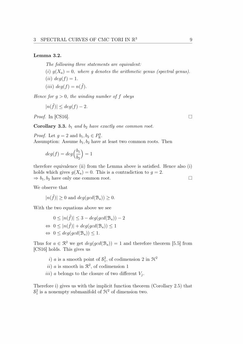
Lemma 3.2.

The following three statements are equivalent:(i) g(Xa) = 0, where g denotes the arithmetic genus (spectral genus).(ii) deg(f) = 1.

(iii) deg(f) = n(f).

Hence for g > 0, the winding number of f obeys

|n(f)| ≤ deg(f)− 2.

Proof. In [CS16].

Corollary 3.3. b1 and b2 have exactly one common root.

Proof. Let g = 2 and b1, b2 ∈ P 3R.

Assumption: Assume b1, b2 have at least two common roots. Then

deg(f) = deg(b1

b2

)= 1

therefore equivalence (ii) from the Lemma above is satisfied. Hence also (i)holds which gives g(Xa) = 0. This is a contradiction to g = 2.⇒ b1, b2 have only one common root.

We observe that

|n(f)| ≥ 0 and deg(gcd(Ba)) ≥ 0.

With the two equations above we see

0 ≤ |n(f)| ≤ 3− deg(gcd(Ba))− 2

⇔ 0 ≤ |n(f)|+ deg(gcd(Ba)) ≤ 1

⇔ 0 ≤ deg(gcd(Ba)) ≤ 1.

Thus for a ∈ R2 we get deg(gcd(Ba)) = 1 and therefore theorem [5.5] from[CS16] holds. This gives us

i) a is a smooth point of S21, of codimension 2 in H2

ii) a is smooth in R2, of codimension 1iii) a belongs to the closure of two different Vj.

Therefore i) gives us with the implicit function theorem (Corollary 2.5) thatS2

1 is a nonempty submanifold of H2 of dimension two.


3.2 The closure of P2

We want to determine P2. In fact we will see the following Lemma.

Lemma 3.4.

R2 = P2 = S2

The proof resembles some of the key outcomes of [CS16].

Proof. First of all we are going to look at the set R2. We notice that thecondition that all b ∈ Ba have a common root is equivalent to gcd(deg(B2)) ≥1. Thus

R2 ={a ∈ H2 | deg(gcd(Ba)) ≥ 1}Cor. 3.3

= {a ∈ H2 | deg(gcd(Ba)) = 1}

=⋃λ0∈S1{a ∈ H2 | b1(λ0) = 0 = b2(λ0)}

=S2

.

Now it remains to show that also P2 is equal to both sets. Therefore we wantto show that

i) P2 ⊆ R2

ii) S2 ⊆ P2.

The first point i) is a consequence of chapter five of [CS16]. The four con-ditions [A-D] force a ∈ P2 to be in R2. The second point ii) follows directlybecause any sym point λ0 is contained in the unit circle S1. Thus we obtainequality throughout these sets.

This only holds true for the spectral genus two. For higher spectral genusthe conjecture of [CS16] gives that only Sg ⊂ Rg holds and hence equalitycannot be proved.

4 WHITHAM DEFORMATIONS 11

4 Whitham deformationsThis chapter is mainly based on chapter 4 from[CS16]. We will now use theso-called Whitham deformations to construct two vector fields with certainconditions from (a, b1, b2) 7−→ (a, b1, b2). The vector (a, b1, b2) denotes thetangent vector at t = 0 and preserves the periods of Θb1 and Θb2 . Sincethe meromorphic differential forms d

dt

∣∣t=0

Θb1 and ddt

∣∣t=0

Θb2 have vanishingperiods and no residues there exist meromorphic functions q1 and q2 on theRiemann surface Xa that satisfy

dqk =d

dt

∣∣∣∣t=0

Θbk

for k = 1, 2. This gives

qk =ick(λ)

y

with ck ∈ P 3R and y =

√λa(λ). Together with the equation above we get the

Whitham equation

∂

∂λ

ick(λ)

y=

∂

∂t

bk(λ)

yλ

∣∣∣∣t=0

.

Using product and chain rule we get the following expression

ic′k(λ)y − ick(λ)y′

y2=bk(λ)yλ− bk(λ)yλ

(yλ)2

here a dot (e.g. a) denotes the derivative with respect to t, evaluated att = 0 and a prime (e.g. a′) denotes the derivative with respect to λ. By thedefinition of y we get

ic′k(λ)√λa(λ)− ick(λ)(a(λ)+λa′(λ)

2√λa(λ)

)

λa(λ)=bkλ√λa(λ)− bk(λ)( λ2a(λ)

2√λa(λ)

)

λ2λa(λ).

This term can be transformed into

ic′k(λ)√λa(λ)

− ick(a(λ) + λa′(λ))

2√λa(λ)

3 =bk(λ)

λ√λa(λ)

− bk(λ)a(λ)

2√λa(λ)

3 .

Multiplying both sides by 2√λa(λ)

3yields

2ic′k(λ)λa(λ)− ick(λ)a(λ)− ickλa′(λ) = 2bk(λ)a(λ)− bka(λ).

12 4 WHITHAM DEFORMATIONS

Therefore for k = 1 we get

(2λac′1 − ac1 − λa′c1)i = 2ab1 − ab1 (1)

and for k = 2

(2λac′2 − ac2 − λa′c2)i = 2ab2 − ab2. (2)

These two equations are exactly equations [7] and [8] from [CS16]. Sinceequation (1) and equation (2) are compatible we can calculate c2·equation(1)-c1·equation (2), which gives us

ic22λac′1 − ic2ac1 − ic2λa′c1 − ic12λac′2 + ic1ac2 + ic1λa

′c2

= c22ab1 − c2ab1 − c12ab2 + c1ab2.

This expression can be simplified to

2a(ic′1c2λ− ic′2c1λ+ c1b2 − c2b1) = a(c1b2 − c2b1).

Therefore both sides need to vanish at all roots of a. If a does not vanish atall roots of a, c1b2− c2b1 needs to vanish at the remaining ones. Additionallyequation (1) and equation (2) yield that c1 and c2 also vanish at the rootsthat a and a have in common. Thus we get the following expression

c1b2 − c2b1 = Qa, (3)

where Q ∈ P 2R. Q also satisfies the reality condition. We have seen how

starting with a given tangent vector (a, b1, b2) one can first use equation (1)and equation (2) to get two polynomials c1, c2 ∈ P 3

R and then secondly solveequation (3) for Q ∈ P 2

R. Our goal is now to reverse this process. To do thiswe will proceed as follows.

1. Solve equation (3) with given (a, b1, b2) ∈ F2and Q ∈ P 2R for c1, c2 ∈ P 3

R.

2. Solve equation (1) and equation (2) with given (a, b1, b2, Q, c1, c2) for

the tangent vector (a, b1, b2).

4.1 Uniqueness of solutions

First of all we are going to prove that we can indeed solve these equationsuniquely with polynomials that satisfy the reality condition. Secondly wewant to explicitly solve them given the values of c1(1), c2(1). We will be ableto derive certain conditions depending on these values such that we can solvethe equations (1)-(3) with unique solutions. The first c1, c2 we are interestedin are such that c1(1) = 1 and c2(1) = 0, while the second c1, c2 are such thatc1(1) = 0 and c2(1) = 1. Additionally we want b1, b2 to have a root at λ = 1.


Lemma 4.1. If the polynomials b1, b2 have a root at λ = 1, then Q also hasa root at λ = 1, i.e. gcd(Ba) divides Q.

Proof. Assume b1, b2 have a root at λ = 1, then equation (3) evaluated atλ = 1 gives us 0 = Q(1)a(1). So either Q or a needs to have a root at λ = 1.Case 1: Q has root of maximal order 2 at λ = 1.This case already implies that Q has a root at λ = 1 and is therefore fairlytrivial.Case 2: a has a root at λ = 1.Due to the distinctness of the roots of a the order of the root λ = 1 is 1.Therefore a′ does not have a root at λ = 1. Evaluating equation (1) at λ = 1then yields −a′(1)c1(1)i = 0. Since a′ cannot have a root at λ = 1 c1 needs tohave a root at λ = 1. The same argumentation applied to equation (2) givesus that also c2 has to have a root at λ = 1. Now the right side of equation(3) has a root at λ = 1 of order 2. Thus Qa also needs to have a root oforder 2 at λ = 1. Since all roots of a only have order 1 Q also needs to havea root at λ = 1.In both cases Q has a root at λ = 1.

Corollary 4.2. If either c1 or c2 has no root at λ = 1 a has no root at λ = 1.

Proof. Assume a has a root at λ = 1, then with the same argumentation asin the proof of Lemma (4.1) we get due to equation (1) and (2) that c1 andc2 have to have a root at λ = 1. This is a contradiction to the prequisite thatone of both has no root at λ = 1 (in fact we want to have c1, c2 such thateither of them is one at λ = 1).

Thus a does not have a root at λ = 1 in the cases we are interested in.

Lemma 4.3. If a, b1 and b2 are such that b1 and b2 have only one commonroot of first order and this root is at λ = 1 and a(1) 6= 0 then there are uniquesolutions of equation (1), (2) and (3) such that b1 and b2 vanish at λ = 1.They are uniquely defined through c1(1) and c2(1).

Proof. If we set λ = 1 in equation (1) we get:

(2a(1)c′1(1)− a(1)c1(1)− a′(1)c1(1))i = 0

⇔ 2a(1)c′1(1) = a(1)c1(1) + a′(1)c1(1)

⇔ c′1(1) =1

2a(1)(a(1)c1(1) + a′(1)c1(1))

⇔ c′1(1) =c1(1)

2+a′(1)c1(1)

2a(1)


And if we set λ = 1 in equation (2) we get:

(2a(1)c′2(1)− a(1)c2(1)− a′(1)c2(1))i = 0

⇔ 2a(1)c′2(1) = a(1)c2(1) + a′(1)c2(1)

⇔ c′2(1) =1

2a(1)(a(1)c2(1) + a′(1)c2(1))

⇔ c′2(1) =c2(1)

2+a′(1)c2(1)

2a(1)

Since we are interested in special c1, c2 we can later explicitly calculate thesepolynomials through these conditions. We will now see that the values ofQ′(1) and Q′′(1) are defined by c1(1) and c2(1). To get this result we willdifferentiate equation (3) with respect to lambda and set λ = 1

c′1b2 + c1b′2 − c′2b1 − c2b

′1 = Q′a+Qa′. (3’)

Setting λ = 1 gives us

c′1(1)b2(1) + c1b′2(1)− c′2(1)b1(1)− c2(1)b′1(1) = Q′(1)a(1) +Q(1)a′(1)

b1(1)=0,b2(1)=0,Q(1)=0⇔ c1(1)b′2(1)− c2(1)b′1(1) = Q′(1)a(1)

⇔ Q′(1) =c1(1)b′2(1)− c2(1)b′1(1)

a(1).

We also want to obtain the second derivative of Q at λ = 1 that is Q′′(1).Therefore we differentiate (3’) with respect to λ to get

c′′1b2 + 2c′1b′2 + c1b

′′2 − c′′2b1 − 2c′2b

′1 − c2b

′′1 = Q′′a+ 2Q′a′ +Qa′′. (3”)

This expression evaluated at λ = 1 together with b1(1) = 0, b2(1) = 0 and


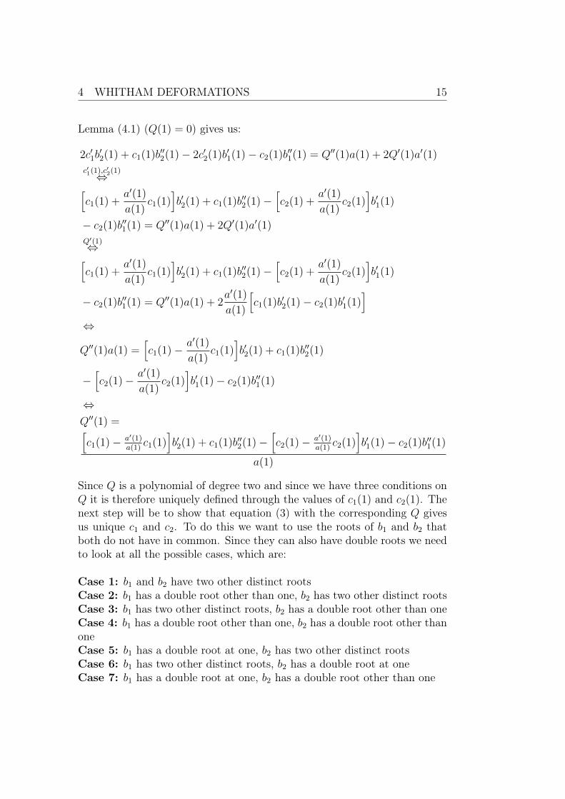
Lemma (4.1) (Q(1) = 0) gives us:

2c′1b′2(1) + c1(1)b′′2(1)− 2c′2(1)b′1(1)− c2(1)b′′1(1) = Q′′(1)a(1) + 2Q′(1)a′(1)

c′1(1),c′2(1)⇔[

c1(1) +a′(1)

a(1)c1(1)

]b′2(1) + c1(1)b′′2(1)−

[c2(1) +

a′(1)

a(1)c2(1)

]b′1(1)

− c2(1)b′′1(1) = Q′′(1)a(1) + 2Q′(1)a′(1)

Q′(1)⇔[c1(1) +

a′(1)

a(1)c1(1)

]b′2(1) + c1(1)b′′2(1)−

[c2(1) +

a′(1)

a(1)c2(1)

]b′1(1)

− c2(1)b′′1(1) = Q′′(1)a(1) + 2a′(1)

a(1)

[c1(1)b′2(1)− c2(1)b′1(1)

]⇔

Q′′(1)a(1) =[c1(1)− a′(1)

a(1)c1(1)

]b′2(1) + c1(1)b′′2(1)

−[c2(1)− a′(1)

a(1)c2(1)

]b′1(1)− c2(1)b′′1(1)

⇔Q′′(1) =[c1(1)− a′(1)

a(1)c1(1)

]b′2(1) + c1(1)b′′2(1)−

[c2(1)− a′(1)

a(1)c2(1)

]b′1(1)− c2(1)b′′1(1)

a(1)

Since Q is a polynomial of degree two and since we have three conditions onQ it is therefore uniquely defined through the values of c1(1) and c2(1). Thenext step will be to show that equation (3) with the corresponding Q givesus unique c1 and c2. To do this we want to use the roots of b1 and b2 thatboth do not have in common. Since they can also have double roots we needto look at all the possible cases, which are:

Case 1: b1 and b2 have two other distinct rootsCase 2: b1 has a double root other than one, b2 has two other distinct rootsCase 3: b1 has two other distinct roots, b2 has a double root other than oneCase 4: b1 has a double root other than one, b2 has a double root other thanoneCase 5: b1 has a double root at one, b2 has two other distinct rootsCase 6: b1 has two other distinct roots, b2 has a double root at oneCase 7: b1 has a double root at one, b2 has a double root other than one


Case 8: b1 has a double root other than one, b2 has a double root at oneCase 9: one of the bk has a triple root at λ = 1 for k = 1, 2

Case 1: Let b1 have two distinct roots at β11 and β12 and let b2 have twodistinct roots at β21 and β22. Now let us look at equation (3) evaluated atthese roots. (3) evaluated at λ = β11 yields

c1(β11)b2(β11) = Q(β11)a(β11)

c1(β11) =Q(β11)a(β11)

b2(β11)

for λ = β12 we get

c1(β12)b2(β12) = Q(β12)a(β12)

c1(β12) =Q(β12)a(β12)

b2(β12).

Together with the value of c1(1) and the derivative c′1(1) we obtain fourconditions on c1(λ):

I. c1(1)

II. c′1(1) =c1(1)

2+a′(1)

2a(1)c1(1)

III. c1(β11) =Q(β11)a(β11)

b2(β11)

IV. c1(β12) =Q(β12)a(β12)

b2(β12)

Likewise we get the following four conditions for c2, where β21 and β22 denotethe two distinct roots of b2:

I. c2(1)

II. c′2(1) =c2(1)

2+a′(1)

2a(1)c2(1)

III. c2(β21) =Q(β21)a(β21)

b1(β21)

IV. c2(β22) =Q(β22)a(β22)

b1(β22)

Because c1 and c2 are both polynomials of degree three they both have amaximum of four different coefficients that need to be determined. Since we


found four conditions on each of these polynomials we can now solve themto get the desired coefficients. Since we already showed that Q is uniquleydefined by c1(1) and c2(1) the obtained solutions will also be unique. Thuswe obtain unique c1 and c2.

Case 2: Let b1 have a double root at β11 and b2 have two distinct rootsat β21 and β22. Then the conditions on c2 will not change. So we only haveto look at c1. Due to the fact that b1 has a double root at β11 the old condi-tions III and IV are equal. Therefore we need to replace one of them througha new condition. Following the previous reasoning it is intuitive to look atthe derivatives of (3) with respect to λ evaluated at β11, which yields

c′1(β11)b2(β11) + c1(β11)b′2(β11)− c′2(β11)b1(β11)− c2(β11)b′1(β11)

= Q′(β11)a(β11) +Q(β11)a′(β11).

Since b1 has a double root at β11 we get b1(β11) = 0 and b′1(β11) = 0. Thusthe expression above simplifies to

c′1(β11)b2(β11) + c1(β11)b′2(β11) = Q′(β11)a(β11) +Q(β11)a′(β11).

This equation gives us a fourth equation to uniquely determine c1. The fourconditions for c1 in this case are:

I. c1(1)

II. c′1(1) =c1(1)

2+a′(1)

2a(1)c1(1)

III. c1(β11) =Q(β11)a(β11)

b2(β11)

IV. c′1(β11)b2(β11) + c1(β11)b′2(β11) = Q′(β11)a(β11) +Q(β11)a′(β11)

The conditions on c2 remain the same and are therefore:

I. c2(1)

II. c′2(1) =c2(1)

2+a′(1)

2a(1)c2(1)

III. c2(β21) =Q(β21)a(β21)

b1(β21)

IV. c2(β22) =Q(β22)a(β22)

b1(β22)

Case 3: Let b1 have two distinct roots at β11 and β12 and b2 have a double


root at β21. Then we get the converse conditions to case 2. Thus the con-ditions on c1 remain the same as in case 1 and the conditions on c2 can bederived as the conditions for c1 in case 2. Therefore we obtain the followingconditions on c1:

I. c1(1)

II. c′1(1) =c1(1)

2+a′(1)

2a(1)c1(1)

III. c1(β11) =Q(β11)a(β11)

b2(β11)

IV. c1(β12) =Q(β12)a(β12)

b2(β12)

Taking the derivative of equation (3) with respect to λ evaluated at λ = β22

gives us

I. c2(1)

II. c′2(1) =c2(1)

2+a′(1)

2a(1)c2(1)

III. c2(β21) =Q(β21)a(β21)

b1(β21)

IV. c′2(β21)b1(β21) + c2(β21)b′1(β21) = Q′(β21)a(β21) +Q(β21)a′(β21).

Hence we again get that c1 and c2 can be uniquely defined.

Case 4: Let b1 have a double root at β11 and let b2 have a double rootat β21. This is clearly a combination of case 2 and case 3. We can thereforesimply take the conditions on c1 from case 2 and the conditions from case 3on c2 to get that both are uniquely defined. Thus our conditions on c1 are

I. c1(1)

II. c′1(1) =c1(1)

2+a′(1)

2a(1)c1(1)

III. c1(β11) =Q(β11)a(β11)

b2(β11)



While the conditions on c2 are:

I. c2(1)

II. c′2(1) =c2(1)

2+a′(1)

2a(1)c2(1)

III. c2(β21) =Q(β21)a(β21)

b1(β21)


Case 5: Let b1 have a double root at λ = 1 and a single root at λ = β11.While b2 has three distinct roots at λ = 1, β21, β22. The conditions on c2

remain the same, whereas the conditions on c1 differ slightly. Thus we get

I. c1(1)

II. c′1(1) =c1(1)

2+a′(1)

2a(1)c1(1)

III. c1(β11) =Q(β11)a(β11)

b2(β11)

IV. c′1(1)b2(1) + c1(1)b′2(1) = Q′(1)a(1) +Q(1)a′(1)

andI. c2(1)

II. c′2(1) =c2(1)

2+a′(1)

2a(1)c2(1)

III. c2(β21) =Q(β21)a(β21)

b1(β21)

IV. c2(β22) =Q(β22)a(β22)

b1(β22).

Case 6: Let b2 have a double root at λ = 1 and a single root at λ = β21.While b1 has three distinct roots at λ = 1, β11, β12. The conditions on c1

remain the same, whereas the conditions on c2 differ slightly. Thus we get

I. c1(1)

II. c′1(1) =c1(1)

2+a′(1)

2a(1)c1(1)

III. c1(β11) =Q(β11)a(β11)

b2(β11)

IV. c1(β12) =Q(β12)a(β12)

b2(β12)


and

I. c2(1)

II. c′2(1) =c2(1)

2+a′(1)

2a(1)c2(1)

III. c2(β21) =Q(β21)a(β21)

b1(β21)

IV. c′2(1)b1(1) + c2(1)b′1(1) = Q′(1)a(1) +Q(1)a′(1).

Case 7: Let b1 have a double root at λ = 1 and a single root at λ = β11.While b2 has a single root at λ = 1 and a double root at λ = β21. This is acombination of case (3) and (5). Thus we get

I. c1(1)

II. c′1(1) =c1(1)

2+a′(1)

2a(1)c1(1)

III. c1(β11) =Q(β11)a(β11)

b2(β11)

IV. c′1(1)b2(1) + c1(1)b′2(1) = Q′(1)a(1) +Q(1)a′(1)

and

I. c2(1)

II. c′2(1) =c2(1)

2+a′(1)

2a(1)c2(1)

III. c2(β21) =Q(β21)a(β21)

b1(β21)


Case 8: Let b1 have a double root at β11 and b2 have a double root atλ = 1 and a single root at β21. Since this combines case 2 and case 6 we get

I. c1(1)

II. c′1(1) =c1(1)

2+a′(1)

2a(1)c1(1)

III. c1(β11) =Q(β11)a(β11)

b2(β11)



and

I. c2(1)

II. c′2(1) =c2(1)

2+a′(1)

2a(1)c2(1)

III. c2(β21) =Q(β21)a(β21)

b1(β21)

IV. c′2(1)b1(1) + c2(1)b′1(1) = Q′(1)a(1) +Q(1)a′(1).

Case 9: Since bk has a triple root at λ = 1 we need to find another fourthcondition on ck for k = 1, 2. While c3−k is already uniquley defined throughany of the conditions form case 1-8. We can find the additional condition forck through equation (3”) evaluated at λ = 1. Thus we get:

I. ck(1)

II. c′k(1) =c1(1)

2+a′(1)

2a(1)c1(1)

III. c′k(1)b3−k(1) + ck(1)b′3−k(1) = Q′(1)a(1) +Q(1)a′(1)

IV : c′′k(1)b3−k(1) + 2c′k(1)b′3−k(1) + ckb′′2(1)

= Q′′(1)a(1) + 2Q′(1)a′(1) +Qa′′(1)

Since b1 and b2 can only have exactly one common root due to Corollary (3.3)and we require that this common root is at λ = 1 we covered all possiblecases. And since all cases yield unique solutions for c1 and c2 we can alwaysobtain a unique solution. The next and final step to get the result that wecan uniquely solve equations (1),(2) and (3) for a, b1 and b2 is to simply solveequations (1) and (2) for these polynomials with the derived polynomials c1

and c2. We will start by determining a. Since a(λ) =∏2

j=1

ηj|ηj |(λ−ηj)(λ−η

−1j )

all we need to do is to find η1, η2. Since the complex conjugation commuteswith differentiation with respect to real variables this will immediately implyη−1

1 , η−1

2 and therefore a. We will first calculate the derivatives of a withrespect to λ and with respect to t eveluated at t = 0.

a′(λ) =η1η2

|η1||η2|((λ− η−1

1 )(λ− η2)(λ− η−12 ) + (λ− η1)(λ− η2)(λ− η−1

2 )

+ (λ− η1)(λ− η−11 )(λ− η−1

2 ) + (λ− η1)(λ− η−11 )(λ− η2))


and

a(λ) =(η1η2 + η1η2)|η1||η2| − η1η2( ˙|η1||η2|+ |η1| ˙|η2|)

(|η1||η2|)2((λ− η1)(λ− η−1

1 )

(λ− η2)(λ− η−12 )) +

η1η2

|η1||η2|(−η1(λ− η−1

1 )(λ− η2)(λ− η−12 )

− η−1

1 (λ− η1)(λ− η2)(λ− η−12 )− η2(λ− η1)(λ− η−1

1 )(λ− η−12 )

− η−1

2 (λ− η1)(λ− η−11 )(λ− η2))

Equation (1) and (2) suggest now to evaluate both at the roots of a, whichare η1, η2, η

−11 , η−1

2 . From the calculations above we get e.g. for λ = η1

a′(η1) =η1η2

|η1||η2|(η1 − η−1

1 )(η1 − η2)(η1 − η−12 ).

and

a(η1) =η1η2

|η1||η2|(−η1)(η1 − η−1

1 )(η1 − η2)(η1 − η−12 )

⇒ a(η1) =− η1a′(η1)

likewise for η2, η−11 and η−1

2

a(η2) =− η2a′(η2)

a(η−11 ) =− η−1

1 a′(η−11 )

a(η−12 ) =− η−1

2 a′(η−12 ).

By looking at a one may realize that it suffices to calculate η1 and η2. Toobtain these one can use equation (1) or equation (2) both yield similarresults. We will evaluate the respective equation at either η1 or η2. Withoutloss of generality we will use equation (1).

(2η1a(η1)c′1(η1)− a(η1)c1(η1)− η1a′(η1)c1(η1))i =2a(η1)b1(η1)− a(η1)b1(η1)

⇔ −η1a′(η1)c1(η1)i =− a(η1)b1(η1)

a(ηk)=−ηka′(ηk)⇔ −η1a′(η1)c1(η1)i =η1a

′(η1)b1(η1)

⇔ η1 =−η1a

′(η1)c1(η1)i

a′(η1)b1(η1)

⇔ η1 =−η1c1(η1)i

b1(η1)


With the same calculations one gets

−η2a′(η2)c1(η2)i =− a(η2)b1(η2)

a(ηk)=−ηka′(ηk)⇔ −η2a′(η2)c1(η2)i =η2a

′(η2)b1(η2)

⇔ η2 =−η2a

′(η2)c1(η2)i

a′(η2)b1(η2)

⇔ η2 =−η2c1(η2)i

b1(η2).

These calculations with equation (2) yield

η1 =−η1c2(η1)i

b2(η1)

and

η2 =−η2c2(η2)i

b2(η2).

This acutally provides a nice backcheck with equation (3), which eveluatedat ηk yields

c1(ηk)b2(ηk)− c2(ηk)b1(ηk) =0

⇔ c1(ηk)b2(ηk) =c2(ηk)b1(ηk)

⇔ c1(ηk)

b1(ηk)=c2(ηk)

b2(ηk).

Since we can now write a(λ) down we automatically get b1(λ) from equation(1) and b2(λ) from equation (2). Which are as follows

(2λac′1 − ac1 − λa′c1)i = 2ab1 − ab1

⇔(2λac′1 − ac1 − λa′c1)i+ ab1

2a= b1

and

(2λac′2 − ac2 − λa′c2)i = 2ab2 − ab2

⇔(2λac′2 − ac2 − λa′c2)i+ ab2

2a= b2

Since we uniquely determined c1, c2 and a above we also get uniquely definedb1, b2. Thus we have finally proved Lemma (4.3).


Corollary 4.4. If ck vanishes at λ = 1 then so does c′k, whilst c′l = 12

+ a′(1)a(1)

for k = 1, 2 and l 6= k.

Proof. Let without loss of generality c1(1) = 1 and c2(1) = 0. We will nowevaluate equation (1) and (2) at λ = 1. Equation (1) yields

2a(1)c′1(1)− a(1)c1(1)− a′(1)c1(1) = 0

⇔ 2a(1)c′1 = a(1)c1(1) + a′(1)c1(1)

c1(1)=1⇔ c′1(1) =1

2+a′(1)

a(1).

Equation (2) yields

2a(1)c′2(1)− a(1)c2(1)− a′(1)c2(1) = 0

⇔2a(1)c′2(1) = a(1)c2(1) + a′(1)c2(1)

c2(1)=0⇔ c′2(1) = 0.

It remains to show that Q, c1 and c2 satisfy the reality condition. To do thiswe will use the conditions obtained in the proof of Lemma (4.3). First of allwe will prove some basic facts about polynomials of degree three that satisfythe reality condition.

Lemma 4.5. Let p ∈ P 3R therefore p is a polynomial of degree three that

satisfies the reality condition λ3p(λ−1) = p(λ). Then p also satisfies:

i) p(1) ∈ R

ii) (p′(1)− 3

2p(1)) ∈ iR

iii) i=(p′′(1)) = 2p′(1)− 3p(1)

Proof. Since p satisfies the reality condition we know that it has the formp3λ

3 + p2λ2 + p2λ+ p3 with p3, p2 ∈ C

i) Thus p(1) = p3 + p2 + p2 + p3 = 2<(p3) + 2<(p20) ∈ R.

ii) By differentiating p with respect to λ we get p′(λ) = 3p3λ2 + 2p2λ+ p2.

Thus

p′(1)− 3

2p(1) =3p3 + 2p2 + p2 −

3

2p3 −

3

2p2 −

3

2p2 −

3

2p3

=3i=(p3) + i=(p2) ∈ iR


iii) By differentiating p′ with respect to λ we get p′′(λ) = 6p3λ + 2p2. Wethen observe that

p′′(1) =6p3 + 2p2 = 6<(p3) + 6i=(p3) + 2<(p2) + 2i=(p2),

⇒ i=(p′′(1)) =6i=(p3) + 2i=(p2)

p′(1) =3p3 + 2p2 + p2 = 3<(p3) + 3i=(p3) + 3<(p2) + i=(p2)

p(1) =2<(p3) + 2<(p2)

⇒ 2p′(1)− 3p(1) =6i=(p3) + 2i=(p2) = i=(p′′(1)).

Lemma 4.6. The polynomial Q satisfies the reality condition.

Proof. From the conditions on Q we get:

Q(λ) = (1− λ)Q′(1) + (1− λ)2Q′′(1)

2

=Q′′(1)

2λ2 + (Q′′(1)−Q′(1))λ+Q′(1) +

Q′′(1)

2

with

Q′(1) =c1(1)b′2(1)− c2(1)b′1(1)

a(1)

and

Q′′(1) =[c1(1)− a′(1)

a(1)c1(1)

]b′2(1) + c1(1)b′′2(1)−

[c2(1)− a′(1)

a(1)c2(1)

]b′1(1)− c2(1)b′′1(1)

a(1)

The reality condition λ2Q(λ−1) = Q(λ) is equivalent to

Q′(1) ∈ iRQ′(1)−Q′′(1) ∈ R

We observe that true to Lemma (4.5) if c1 and c2 satisfy the reality conditionc1(1) and c2(1) both are real and therefore can be neglected. In fact we areonly interested in the cases c1(1) = 1, c2(1) = 0 and c1(1) = 0, c2(1) = 1, thuswe can focus on the polynomials a, b1 and b2 to check the reality conditions.We immediately get that a(1) and a(1)2 are real. Thus a(1), c1(1) and c2(1)are real. Furthermore, we are in the case that b1(1) = 0 and b2(1) = 0. Since


the polynomials b1 and b2 satisfy the reality conditions Lemma (4.5) holds.Especially (ii) becomes b′1(1) ∈ iR and b′2(1) ∈ iR. Thus c1(1)

a(1)and c2(1)

a(1)are

real. Since the product of a real and an imaginary number is again imaginarywe obtain that Q′(1) = c1(1)

a(1)b′2(1)− c2(1)

a(1)b′1(1) consists of two imaginary terms

and is therefore imaginary.

It remains to show that the imaginary part of Q′(1)−Q′′(1) vanishes. Firstof all we will use a(1)2 as the common denominator of all terms. Thus weget:

c1(1)a(1)

a(1)2− c1(1)

a(1)2a′(1)b′2(1) +

c1(1)a(1)

a(1)a(1)b′′2(1)

−c2(1)a(1)

a(1)2+c2(1)

a(1)2a′(1)b′1(1)− c2(1)a(1)

a(1)a(1)b′′1(1)

Since c1(1)a(1)a(1)2

, c1(1)a(1)2

, c1(1)a(1)a(1)

, c2(1)a(1)a(1)2

, c2(1)a(1)2

and c2(1)a(1)a(1)

are real due to the rea-soning above, it suffices to look at

a′(1)b′1(1)− a(1)b′′1(1)− a′(1)b′2(1) + a(1)b′′2(1).

Now we observe that for a(λ) = a4λ4 +a3λ

3 +a2λ2 +a3λ+a4, with a4, a3 ∈ C

and a2 ∈ R

a(1) = 2<(a4) + 2<(a3) + a2

and

a′(1) = 4<(a4) + 4i=(a4) + 4<(a3) + 2i=(a3) + 2a2

holds. Thus we get <(a′(1)) = 2a(1).

⇒ a′(1)− 2a(1) ∈ iR

If we substitute i=(b′′1(1)) and i=(b′′2(1)) through 2b′1(1)−3b1(1) and 2b′2(1)−3b2(1) as described in Lemma (4.5) (iii) we obtain

a′(1)b′1(1)− a(1)(2b′1(1)− 3b1(1) + <(b′′1(1))

− a′(1)b′2(1) + a(1)(2b′2(1)− 3b2(1) + <(b′′2(1))

=b′1(1)(a′(1)− 2a(1))− a(1)(−3b1(1) + <(b′′1(1))

− b′2(1)(a′(1)− 2a(1)) + a(1)(−3b2(1) + <(b′′2(1)).

Since b1(1) = 0 = b2(1) we get

b′1(1)(a′(1)− 2a(1))− a(1)<(b′′1(1)− b′2(1)(a′(1)− 2a(1)) + a(1)<(b′′2(1)).


Since b′1(1), (a′(1)−2a(1)), b′2(1) and (a′(1)−2a(1)) are imaginary their prod-uct is real and since a(1)<(b′′1(1) and a(1)<(b′′2(1)) are real, the whole termis real. Hence Q satisfies the reality condition.

It only remains now to show that c1 and c2 satisfy the reality conditions aswell. Since both are polynomials of degree three, which are uniquely definedthrough four conditions it suffices to prove that λ3c1(λ−1) and λ3c2(λ−1)satisfy the corresponding four conditions as well. If this is the case thepolynomials have to be the same due to the unqiueness.

Lemma 4.7. If ck(λ) satisfies the four conditions from the proof of Lemma(4.3) then so does ck(λ) := λ3ck(λ−1) for k = 1, 2.

Proof. Let ck for k = 1, 2 be parametrized through

ck(λ) = ck3λ3 + ck2λ

2 + ck1λ+ ck0

⇒ c1(λ) = ck0λ3 + ck1λ

2 + ck2λ+ ck3λ.

The first condition is ck(1) ∈ R. We have to show that this also impliesthat ck(1) ∈ R. Since ck(1) = ck3 + ck2 + ck1 + ck0 is real we know thati=(ck3 + ck2 + ck1 + ck0) = 0. This implies that −i=(ck3 + ck2 + ck1 + ck0) = 0,which is i=(ck3 + ck2 + ck1 + ck0). Therefore we see that ck(1) = ck3 + ck2 +ck1 + ck0 = ck3 + ck2 + ck1 + ck0 = ck(1). Hence the first condition satisfiesthe reality condition.

The second condition refers to the derivative of ck at λ = 1. We wantto show that

c′k(1) =1

2ck(1) +

a′(1)

2a(1)ck(1) = ck

′(1)

with

ck = λ3ck(λ−1).

To do this we will parametrize ck again as follows

ck = ck3λ3 + ck2λ

2 + ck1λ+ ck0

⇒ c′k(λ) = 3ck3λ2 + 2ck2λ

2 + ck1

⇒ c′k(λ) = 3ck0λ2 + 2ck1λ+ ck2.

Thus c′k(1) = 12ck(1) + a′(1)

2a(1)ck(1) becomes

3ck3 + 2ck2 + ck1 =1

2(ck3 + ck2 + ck1 + ck0) +

a′(1)

2a(1)(ck3 + ck2 + ck1 + ck0).


From the proof of Lemma (4.6) we remember that <(a′(1)) = 2a(1). Apllyingthis we get:

3ck3 + 2ck2 + ck1 =1

2(ck3 + ck2 + ck1 + ck0)

+2a(1) + i=(a′(1))

2a(1)(ck3 + ck2 + ck1 + ck0)

⇔ 3ck3 + 2ck2 + ck1 =3

2(ck3 + ck2 + ck1 + ck0)

+i=(a′(1))

2a(1)(ck3 + ck2 + ck1 + ck0)

⇔ 3

2ck3 +

1

2ck2 −

1

2ck1 −

3

2ck0 =

i=(a′(1))

2a(1)ck(1)

Since ck(1), a(1) ∈ R the right-hand side is imaginary hence we get <(32ck3 +

12ck2 − 1

2ck1 − 3

2ck0) = 0. Thus

i=(3

2ck3 +

1

2ck2 −

1

2ck1 −

3

2ck0) =

i=(a′(1))

2a(1)c1(1)

⇔ 3

2i=(ck3) +

1

2i=(ck2)− 1

2i=(ck1)− 3

2i=(ck0) =

i=(a′(1))

2a(1)ck(1)

¯⇔ − 3

2i=(ck3)− 1

2i=(ck2) +

1

2i=(ck1) +

3

2i=(ck0) = −i=(a′(1))

2a(1)ck(1)

⇔ 3

2ck3 +

1

2ck2 −

1

2ck1 −

1

2ck0 = −i=(a′(1))

2a(1)ck(1)

⇔ − 3ck0 − 2ck1 − ck2 +3

2(ck3 + ck2 + ck1 + ck0) = −i=(a′(1))

2a(1)ck(1)

⇔ − 3ck0 − 2ck1 − ck2 = −1

2ck(1)− ck(1)− i=(a′(1))

2a(1)ck(1)

ck(1)=ck(1)⇔ −3ck0 − 2ck1 − ck2 = −1

2ck(1)− 2a(1)

2a(1)ck(1)− i=(a′(1))

2a(1)ck(1)

2a(1)==(a′(1))⇔ − 3ck0 − 2ck1 − ck2 = −1

2ck(1)− a′(1)

2a(1)ck(1)

⇔ − c′k(1) = −1

2ck(1)− a′(1)

2a(1)ck(1)

·(−1)⇔ c′k(1) =1

2ck(1) +

a′(1)

2a(1)ck(1)

⇔ c′k(1) = c′k(1)

Thus the second condition satisfies the reality condition.


The third and fourth condition in the case that polynomial bk has distinctroots can be seen from equation (3). Let β denote any root other than oneof the polynomial bk. First of all we observe that

bk(β) = 0reality condition⇒ β3bk(β−1) = 0⇒ bk(β−1) = 0.

We know that:

ck(β) =Q(β)a(β)

b3−k(β)

⇔ck(β) =β6Q(β−1)a(β−1)

β3b3−k(β−1)

⇔β−3ck(β) =Q(β−1)a(β−1)

b3−k(β−1)

We will now look at equation (3) and start with λ = β−1. Thus bk vanishesand we obtain

ck(β−1)b3−k(β−1) = Q(β−1)a(β−1)

⇔ck(β−1) =Q(β−1)a(β−1)

b3−k(β−1).

With both calculations together we get

ck(β−1) = β−3ck(β)

⇔β3ck(β−1) = ck(β).

Since this holds for both β = βk1 and β = βk2 the third and fourth conditionalso satisfy the reality condition. Thus in this case the reality condition issatisfied and c1 and c2 satisfy the reality condition due to uniqueness. Itremains to look at the case when any of the two polynomials b1 or b2 has adouble root. Since these cases are just limit cases of the case treated above weget a term fully dependend on polynomials that satisfy the reality condition.Thus it satisfies the reality condition. Hence c1 and c2 satisfy the realitycondition in any of the eight cases from the proof of Lemma (4.3).

4.2 Vector field V1

We now want to apply Lemma (4.3) for given c1(1), c2(1). Let V1 denote thevector field corresponding to the conditions c1(1) = 1 and c2(1) = 0. We just


proved additional conditions for (a, b1, b2, Q, c1, c2) such that we can solveequations (1),(2) and (3) to obtain (a, b1, b2), which is exactly what we aregoing to do. First of all a short overview of all conditions:

1. b1(1) = 0, b1(1) = 0

2. b2(1) = 0, b2(1) = 0

3. c1(1) = 1

4. c2(1) = 0

5. Q(1) = 0

6. a(1) 6= 0

7. all polynomials satisfy the reality condition8. c1, c2 satisfy the additional conditions from the proof of Lemma (4.3)

From these conditions we can immediately see what the polynomials b1, b2, Qlook like. That is

b1 = (λ− 1)(b10λ2 + b11λ+ b12), where b10, b11, b12 ∈ C

b2 = (λ− 1)(b20λ2 + b21λ+ b22), where b20, b21, b22 ∈ C

Q = (λ− 1)(q0λ+ q1), where q0, q1 ∈ C.

The first step is now to find aQ that satisfies all these conditions from Lemma(4.3) to solve equation (3) for c1, c2.

Q = (λ− 1)(q0λ+ q1)

= q0λ2 + q1λ− q0λ− q1

Hence we obtain

Q′(λ) = 2q0λ+ q1 − q0

⇒Q′(1) = q0 + q1

Q′′(λ) = 2q0

⇒Q′′(1) = 2q0.

The conditions from the Lemma were:

I. Q′(1) =c1(1)b′2(1)− c2(1)b′1(1)

a(1)

II. Q′′(1) =[c1(1)− a′(1)

a(1)c1(1)

]b′2(1) + c1(1)b′′2(1)−

[c2(1)− a′(1)

a(1)c2(1)

]b′1(1)− c2(1)b′′1(1)

a(1)


Given c1(1) = 1 and c2(1) = 0 we get

I. Q′(1) =b′2(1)

a(1)

II. Q′′(1) =

[1− a′(1)

a(1)

]b′2(1) + b′′2(1)

a(1)

Thus we get

q0 + q1 =b′2(1)

a(1)

2q0 =

[1− a′(1)

a(1)

]b′2(1) + b′′2(1)

a(1).

This yields

q0 =

[1− a′(1)

a(1)

]b′2(1) + b′′2(1)

2a(1)

and therefore

q1 =b′2(1)

a(1)− q0

⇒q1 =b′2(1)

a(1)−

[1− a′(1)

a(1)

]b′2(1) + b′′2(1)

2a(1)

⇒q1 =2b′2(1)−

[1− a′(1)

a(1)

]b′2(1)− b′′2(1)

2a(1)

⇒q1 =

[1 + a′(1)

a(1)

]b′2(1)− b′′2(1)

2a(1).

Hence we obtain Q as follows

Q(λ) = (λ− 1)(q0λ+ q1)

⇔Q(λ) = (λ− 1)([1− a′(1)

a(1)

]b′2(1) + b′′2(1)

2a(1)λ+

[1 + a′(1)

a(1)

]b′2(1)− b′′2(1)

2a(1)

)

⇒Q(λ) = (λ− 1)

([1− a′(1)

a(1)

]b′2(1) + b′′2(1)

)λ+ [1 + a′(1)

a(1)

]b′2(1)− b′′2(1)

2a(1)(4)


⇒Q(λ) = (λ− 1)(λ+ 1)b′2(1) + (1− λ)a

′(1)a(1)

b′2(1)− (1− λ)b′′2(1)

2a(1). (5)

Before we continue we want to assure that Q satisfies the reality conditionthat is basically Lemma (4.6).

λ2Q(λ−1) =λ2( b′2(1)

2a(1)λ−2 − a′(1)b′2(1)

2a(1)2λ−2 +

b′′2(1)

2a(1)λ−2 +

b′2(1)

2a(1)λ−1

+a′(1)b′2(1)

2a(1)2λ−1 − b′′2(1)

2a(1)λ−1 − b′2(1)

2a(1)λ−1 +

a′(1)b′2(1)

2a(1)2λ−1

− b′′2(1)

2a(1)λ−1 − b′2(1)

2a(1)− a′(1)b′2(1)

2a(1)2+b′′2(1)

2a(1)

)=b′2(1)

2a(1)− a′(1)b′2(1)

2a(1)2+b′′2(1)

2a(1)+a′(1)b′2(1)

a(1)2λ− b′′2(1)

a(1)λ

− b′2(1)

2a(1)λ2 − a′(1)b′2(1)

2a(1)2λ2 +

b′′2(1)

2a(1)λ2

(4.6)=

b′2(1)

2a(1)λ2 − a′(1)b′2(1)

2a(1)2λ2 +

b′′2(1)

2a(1)λ2 +

a′(1)b′2(1)

a(1)2λ− b′′2(1)

a(1)λ

− b′2(1)

2a(1)− a′(1)b′2(1)

2a(1)2+b′′2(1)

2a(1)

=Q(λ)

With this polyonmial of degree 2 we now want to solve equation (3) forpolynomials c1, c2. First of all we are going to use c1(1) = 1 on the conditionsfound in the proof. We limit ourselves to the case where b1 and b2 have twodistinct roots other than one. We did this because all cases led to rather longterms. Thus these calculations only lead to an exemplary vector field. Byapplying Corollary (4.4) we get

I. c1(1) = 1

II. c′1(1) =1

2+a′(1)

2a(1)

III. c1(β11) =Q(β11)a(β11)

b2(β11)

IV. c1(β12) =Q(β12)a(β12)

b2(β12).


The first condition already tells us that:

c1(λ) = 1 + (λ− 1)(c10λ2 + c11λ+ c12)

⇒c′1(λ) = c10λ2 + c11λ+ c12 + (λ− 1)(2c10λ+ c11)

⇒c′1(1) = c10 + c11 + c12

andc1(β11) = 1 + (β11 − 1)(c10β

211 + c11β11 + c12)

c1(β12) = 1 + (β12 − 1)(c10β212 + c11β12 + c12)

Thus it remains to solve the remaining three conditions for the three coef-ficients. First of all let us replace c1 in equations II-IV with its definition.This yields

II. c10 + c11 + c12 =1

2+a′(1)

2a(1)

III. 1 + (β11 − 1)(c10β211 + c11β11 + c12) =

Q(β11)a(β11)

b2(β11)

IV. 1 + (β12 − 1)(c10β212 + c11β12 + c12) =

Q(β12)a(β12)

b2(β12)

⇔

II. c10 + c11 + c12 =1

2+a′(1)

2a(1)

III. c10β211 + c11β11 + c12 =

Q(β11)a(β11)− b2(β11)

b2(β11)(β11 − 1)

IV. c10β212 + c11β12 + c12 =

Q(β12)a(β12)− b2(β12)

b2(β12)(β12 − 1).

344

WHIT

HAM

DEFO

RMATIO

NS

III − II := III ′. c10(β211 − 1) + c11(β11 − 1) =

Q(β11)a(β11)− b2(β11)

b2(β11)(β11 − 1)− 1

2− a′(1)

2a(1)

IV − II := IV ′. c10(β212 − 1) + c11(β12 − 1) =

Q(β12)a(β12)− b2(β12)

b2(β12)(β12 − 1)− 1

2− a′(1)

2a(1)

−β12 − 1

β11 − 1III ′ + IV ′ := IV ′′. c10(β2

12 − 1)− β12 − 1

β11 − 1(β12 − 1)c10 =

Q(β12)a(β12)− b2(β12)

b2(β12)(β12 − 1)− 1

2− a′(1)

2a(1)

− (β12 − 1)(Q(β11)a(β11)− b2(β11))

(β11 − 1)b2(β11)(β11 − 1)+

β12 − 1

2(β11 − 1)+

(β12 − 1)a′(1)

2(β11 − 1)a(1)

⇔ IV ′′. c10(β2

12 − 1)(β11 − 1)− (β12 − 1)(β211 − 1)

β11 − 1=Q(β12)a(β12)− b2(β12)

b2(β12)(β12 − 1)− 1

2− a′(1)

2a(1)

− (β12 − 1)(Q(β11)a(β11)− b2(β11))

(β11 − 1)b2(β11)(β11 − 1)+

β12 − 1

2(β11 − 1)+

(β12 − 1)a′(1)

2(β11 − 1)a(1)

⇔ c10 =β11 − 1

(β212 − 1)(β11 − 1)− (β12 − 1)(β2

11 − 1)

[Q(β12)a(β12)− b2(β12)

b2(β12)(β12 − 1)− 1

2− a′(1)

2a(1)

− (β12 − 1)(Q(β11)a(β11)− b2(β11))

(β11 − 1)b2(β11)(β11 − 1)+

β12 − 1

2(β11 − 1)+

(β12 − 1)a′(1)

2(β11 − 1)a(1)

]

III ′. c11 =1

(β11 − 1)

(Q(β11)a(β11)− b2(β11)

b2(β11)(β11 − 1)− 1

2− a′(1)

2a(1)− (β2

11 − 1)c10

)II. c12 =

1

2+a′(1)

2a(1)− c10 − c11

4W

HIT

HAM

DEFO

RMATIO

NS

35

⇒ c11 =1

(β11 − 1)

(Q(β11)a(β11)− b2(β11)

b2(β11)(β11 − 1)− 1

2− a′(1)

2a(1)

− (β11 − 1)(β211 − 1)

(β212 − 1)(β11 − 1)− (β12 − 1)(β2

11 − 1)

[Q(β12)a(β12)− b2(β12)

b2(β12)(β12 − 1)− 1

2− a′(1)

2a(1)

− (β12 − 1)(Q(β11)a(β11)− b2(β11))

(β11 − 1)b2(β11)(β11 − 1)+

β12 − 1

2(β11 − 1)+

(β12 − 1)a′(1)

2(β11 − 1)a(1)

])

⇒ c12 =1

2+a′(1)

2a(1)− β11 − 1

(β212 − 1)(β11 − 1)− (β12 − 1)(β2

11 − 1)

[Q(β12)a(β12)− b2(β12)

b2(β12)(β12 − 1)− 1

2− a′(1)

2a(1)

− (β12 − 1)(Q(β11)a(β11)− b2(β11))

(β11 − 1)b2(β11)(β11 − 1)+

β12 − 1

2(β11 − 1)+

(β12 − 1)a′(1)

2(β11 − 1)a(1)

]− 1

(β11 − 1)

(Q(β11)a(β11)− b2(β11)

b2(β11)(β11 − 1)− 1

2− a′(1)

2a(1)− (β11 − 1)(β2

11 − 1)

(β212 − 1)(β11 − 1)− (β12 − 1)(β2

11 − 1)[Q(β12)a(β12)− b2(β12)

b2(β12)(β12 − 1)− 1

2− a′(1)

2a(1)− (β12 − 1)(Q(β11)a(β11)− b2(β11))

(β11 − 1)b2(β11)(β11 − 1)+

β12 − 1

2(β11 − 1)+

(β12 − 1)a′(1)

2(β11 − 1)a(1)

])

364

WHIT

HAM

DEFO

RMATIO

NS

c1(λ) = 1 + (λ− 1)

(β11 − 1

(β212 − 1)(β11 − 1)− (β12 − 1)(β2

11 − 1)

[Q(β12)a(β12)− b2(β12)

b2(β12)(β12 − 1)− 1

2− a′(1)

2a(1)

− (β12 − 1)(Q(β11)a(β11)− b2(β11))

(β11 − 1)b2(β11)(β11 − 1)+

β12 − 1

2(β11 − 1)+

(β12 − 1)a′(1)

2(β11 − 1)a(1)

]λ2

+λ

(β11 − 1)

(Q(β11)a(β11)− b2(β11)

b2(β11)(β11 − 1)− 1

2− a′(1)

2a(1)− (β11 − 1)(β2

11 − 1)

(β212 − 1)(β11 − 1)− (β12 − 1)(β2

11 − 1)[Q(β12)a(β12)− b2(β12)

b2(β12)(β12 − 1)− 1

2− a′(1)

2a(1)− (β12 − 1)(Q(β11)a(β11)− b2(β11))

(β11 − 1)b2(β11)(β11 − 1)+

β12 − 1

2(β11 − 1)+

(β12 − 1)a′(1)

2(β11 − 1)a(1)

])+

1

2+a′(1)

2a(1)− β11 − 1

(β212 − 1)(β11 − 1)− (β12 − 1)(β2

11 − 1)

[Q(β12)a(β12)− b2(β12)

b2(β12)(β12 − 1)− 1

2− a′(1)

2a(1)

− (β12 − 1)(Q(β11)a(β11)− b2(β11))

(β11 − 1)b2(β11)(β11 − 1)+

β12 − 1

2(β11 − 1)+

(β12 − 1)a′(1)

2(β11 − 1)a(1)

]− 1

(β11 − 1)

(Q(β11)a(β11)− b2(β11)

b2(β11)(β11 − 1)− 1

2− a′(1)

2a(1)− (β11 − 1)(β2

11 − 1)

(β212 − 1)(β11 − 1)− (β12 − 1)(β2

11 − 1)

[Q(β12)a(β12)− b2(β12)

b2(β12)(β12 − 1)− 1

2− a′(1)

2a(1)− (β12 − 1)(Q(β11)a(β11)− b2(β11))

(β11 − 1)b2(β11)(β11 − 1)+

β12 − 1

2(β11 − 1)+

(β12 − 1)a′(1)

2(β11 − 1)a(1)

]))


Now we want to calculate c2 with the following conditions:

I. c2(1) = 0

II. c′2(1) = 0

III. c2(β21) =Q(β21)a(β21)

b1(β21)

IV. c2(β22) =Q(β22)a(β22)

b1(β22)

The first two conditions yield that c2 has the form

c2(λ) = (λ− 1)2(c20λ+ c21)

⇒c2(β21) = (β21 − 1)2(c20β21 + c21)

⇒c2(β22) = (β22 − 1)2(c20β22 + c21).

Therefore it remains to solve condition III and IV for c20 and c21.

III. (β21 − 1)2(c20β21 + c21) =Q(β21)a(β21)

b1(β21)

IV. (β22 − 1)2(c20β22 + c21) =Q(β22)a(β22)

b1(β22)

⇔

III. (c20β21 + c21) =Q(β21)a(β21)

b1(β21)(β21 − 1)2

IV. (c20β22 + c21) =Q(β22)a(β22)

b1(β22)(β22 − 1)2

III − IV := III ′. c21β21 − c21β22 =Q(β21)a(β21)

b1(β21)(β21 − 1)2− Q(β22)a(β22)

b1(β22)(β22 − 1)2

⇔c21(β21 − β22) =Q(β21)a(β21)

b1(β21)(β21 − 1)2− Q(β22)a(β22)

b1(β22)(β22 − 1)2

⇔c21 =Q(β21)a(β21)

(β21 − β22)b1(β21)(β21 − 1)2− Q(β22)a(β22)

(β21 − β22)b1(β22)(β22 − 1)2

Now IV gives us:

c22 =Q(β21)a(β21)

b1(β21)(β21 − 1)2− c21β22

⇔ c22 =Q(β21)a(β21)

b1(β21)(β21 − 1)2

− β22

( Q(β21)a(β21)

(β21 − β22)b1(β21)(β21 − 1)2− Q(β22)a(β22)

(β21 − β22)b1(β22)(β22 − 1)2

)

384

WHIT

HAM

DEFO

RMATIO

NS

Thus we also obtain c2:

c2(λ) =(λ− 1)2

(( Q(β21)a(β21)

(β21 − β22)b1(β21)(β21 − 1)2− Q(β22)a(β22)

(β21 − β22)b1(β22)(β22 − 1)2

)λ+

Q(β21)a(β21)

b1(β21)(β21 − 1)2

− β22

( Q(β21)a(β21)

(β21 − β22)b1(β21)(β21 − 1)2− Q(β22)a(β22)

(β21 − β22)b1(β22)(β22 − 1)2

))

Using the definition of Q we get:

c2(λ) =(λ− 1)2

(((β21 − 1)([

1− a′(1)a(1)

]b′2(1) + b′′2(1)

)β21 + [1 + a′(1)

a(1)

]b′2(1)− b′′2(1)a(β21)

2a(1)(β21 − β22)b1(β21)(β21 − 1)2

−(β22 − 1)

([1− a′(1)

a(1)

]b′2(1) + b′′2(1)

)β22 + [1 + a′(1)

a(1)

]b′2(1)− b′′2(1)a(β22)

2a(1)(β21 − β22)b1(β22)(β22 − 1)2

)λ

+(β21 − 1)

([1− a′(1)

a(1)

]b′2(1) + b′′2(1)

)β21 + [1 + a′(1)

a(1)

]b′2(1)− b′′2(1)a(β21)

2a(1)b1(β21)(β21 − 1)2

− β22

((β21 − 1)([

1− a′(1)a(1)

]b′2(1) + b′′2(1)

)β21 + [1 + a′(1)

a(1)

]b′2(1)− b′′2(1)a(β21)

2a(1)(β21 − β22)b1(β21)(β21 − 1)2

−(β22 − 1)

([1− a′(1)

a(1)

]b′2(1) + b′′2(1)

)β22 + [1 + a′(1)

a(1)

]b′2(1)− b′′2(1)a(β22)

2a(1)(β21 − β22)b1(β22)(β22 − 1)2

))


The remaining step to obtain V1 is to solve equation (1) and (2) for a, b1, b2.From Lemma (4.3) we can take the derivatives of η with respect to t eveluatedat t = 0. Which were

η1 =−η1c1(η1)i

b1(η1)

˙η−11 =

−η−11 c1(η−1

1 )i

b1(η−11 )

η2 =−η2c1(η2)i

b1(η2)

˙η−12 =

−η−12 c1(η−1

2 )i

b1(η−12 )

we can calculate ˙|ηk| with chain rule

˙|ηk| =ηk|ηk|

ηk

for k = 1, 2. Since the derivation with respect to t, which is a real variable,and the complex conjugation commute we get

ηk = ηk ⇒ ηk =−ηkc1(ηk)i

b1(ηk)for k = 1, 2.

Now we can use the expression for a from the proof of Lemma (4.3), whichwas

a(λ) =(η1η2 + η1η2)|η1||η2| − η1η2( ˙|η1||η2|+ |η1| ˙|η2|)

(|η1||η2|)2((λ− η1)(λ− η−1

1 )

(λ− η2)(λ− η−12 )) +

η1η2

|η1||η2|(−η1(λ− η−1

1 )(λ− η2)(λ− η−12 )

− η−1

1 (λ− η1)(λ− η2)(λ− η−12 )− η2(λ− η1)(λ− η−1

1 )(λ− η−12 )

− η−1

2 (λ− η1)(λ− η−11 )(λ− η2)).

Using the derived expressions for the derivatives of the absolute value andthe complex conjugation we get

a(λ) =

(−η1c1(η1)ib1(η1)

η2 + η1−η2c1(η2)ib1(η2)

)|η1||η2| − η1η2( η1|η1| η1|η2|+ |η1| η2|η2|)

(|η1||η2|)2

|η1||η2|η1η2

a(λ)

+η1η2

|η1||η2|(−η1(λ− η−1

1 )(λ− η2)(λ− η−12 )− η−1

1 (λ− η1)(λ− η2)(λ− η−12 )

− η2(λ− η1)(λ− η−11 )(λ− η−1

2 )− η−1

2 (λ− η1)(λ− η−11 )(λ− η2)).


Finally we plug in the derivatives of the roots of a with respect to t to get a.

a(λ) =

(−η1c1(η1)ib1(η1)

η2 + η1−η2c1(η2)ib1(η2)

)|η1||η2| − η1η2( η1|η1|−η1c1(η1)ib1(η1)

|η2|+ |η1| η2|η2|−η2c1(η2)ib1(η2)

)

(|η1||η2|)2

|η1||η2|η1η2

a(λ) +η1η2

|η1||η2|(−−η1c1(η1)i

b1(η1)(λ− η−1

1 )(λ− η2)(λ− η−12 )

− −η−11 c1(η−1

1 )i

b1(η−11 )

(λ− η1)(λ− η2)(λ− η−12 )− −η2c1(η2)i

b1(η2)(λ− η1)

(λ− η−11 )(λ− η−1

2 )− −η−12 c1(η−1

2 )i

b1(η−12 )

(λ− η1)(λ− η−11 )(λ− η2)).

(6)

Since we can now write a(λ) down we automatically get b1(λ) from equation(1) and b2(λ) from equation (2). Which are as follows

(2λac′1 − ac1 − λa′c1)i = 2ab1 − ab1

⇔(2λac′1 − ac1 − λa′c1)i+ ab1

2a= b1

⇔ b1 =(2λac′1 − ac1 − λa′c1)i

2a+b1

a2a (7)

and

(2λac′2 − ac2 − λa′c2)i = 2ab2 − ab2

⇔(2λac′2 − ac2 − λa′c2)i+ ab2

2a= b2

⇔ b2 =(2λac′2 − ac2 − λa′c2)i

2a+b2

2aa. (8)

4W

HIT

HAM

DEFO

RMATIO

NS

41

b1 =(2λac′1 − ac1 − λa′c1)i

2a+b1

2a

(−η1c1(η1)ib1(η1)

η2 + η1−η2c1(η2)ib1(η2)

)|η1||η2| − η1η2( η1|η1|−η1c1(η1)ib1(η1)

|η2|+ |η1| η2|η2|−η2c1(η2)ib1(η2)

(|η1||η2|)2)

|η1||η2|η1η2

a(λ) +η1η2

|η1||η2|(−−η1c1(η1)i

b1(η1)(λ− η−1

1 )(λ− η2)(λ− η−12 )− −η

−11 c1(η−1

1 )i

b1(η−11 )

(λ− η1)(λ− η2)(λ− η−12 )

− −η2c1(η2)i

b1(η2)(λ− η1)(λ− η−1

1 )(λ− η−12 )− −η

−12 c1(η−1

2 )i

b1(η−12 )

(λ− η1)(λ− η−11 )(λ− η2))

b2 =(2λac′2 − ac2 − λa′c2)i

2a+b2

2a

(−η1c1(η1)ib1(η1)

η2 + η1−η2c1(η2)ib1(η2)

)|η1||η2| − η1η2( η1|η1|−η1c1(η1)ib1(η1)

|η2|+ |η1| η2|η2|−η2c1(η2)ib1(η2)

)

(|η1||η2|)2

|η1||η2|η1η2

a(λ) +η1η2

|η1||η2|(−−η1c1(η1)i

b1(η1)(λ− η−1

1 )(λ− η2)(λ− η−12 )− −η

−11 c1(η−1

1 )i

b1(η−11 )

(λ− η1)(λ− η2)(λ− η−12 )

− −η2c1(η2)i

b1(η2)(λ− η1)(λ− η−1

1 )(λ− η−12 )− −η

−12 c1(η−1

2 )i

b1(η−12 )

(λ− η1)(λ− η−11 )(λ− η2)).


4.3 Vector field V2

We want to proceed almost like in 4.1 to get another vector field, which wewill call V2. We will again limit ourselves on the case that b1 and b2 have twodistinct roots other than one. Thus the obtained vector field is again onlyexemplary. This time we want to have c1(1) = 0 and c2(1) = 1. Thus manyof the conditions from 4.1 simply switch to the other corresponding equation.This gives us the following conditions:

1. b1(1) = 0, b1(1) = 0

2. b2(1) = 0, b2(1) = 0

3. c1(1) = 0

4. c2(1) = 1

5. Q(1) = 0

6. a(1) 6= 0

7. all polynomials satisfy the reality condition8. c1, c2 satisfy the additional conditions from the proof of Lemma (4.3)

We already now that Q has the form

Q(λ) = (λ− 1)(q0λ+ q0) , where q0, q1 ∈ C.

We also know that

Q′(1) = q0 + q1

and

Q′′(1) = 2q0.

Now we want to repeat the procedure from the proof of Lemma 4.3, wherewe differentiated equation (3) with respect to λ and then evaluated it at 1.Thus we get

q0 + q1 =b1(1)

a(1)

and

2q0 =

[1− a′(1)

a(1)

]b′1(1) + b′′1(1)

a(1).


The latter yields

q0 =

[1− a′(1)

a(1)

]b′1(1) + b′′1(1)

2a(1).

Which in return gives us

q1 =b1(1)

a(1)− q0

⇒ q1 =b1(1)

a(1)−

[1− a′(1)

a(1)

]b′1(1) + b′′1(1)

2a(1)

⇒ q1 =

[1 + a′(1)

a(1)

]b′1(1)− b′′1(1)

2a(1).

Therefore we can already write down Q corresponding to V2.

Q(λ) = (λ− 1)(q0λ+ q1)

⇔Q(λ) = (λ− 1)([1− a′(1)

a(1)

]b′1(1) + b′′1(1)

2a(1)λ+

[1 + a′(1)

a(1)

]b′1(1)− b′′1(1)

2a(1)

)

⇒Q(λ) = (λ− 1)

([1− a′(1)

a(1)

]b′1(1) + b′′1(1)

)λ+ [1 + a′(1)

a(1)

]b′1(1)− b′′1(1)

2a(1)(9)

⇒Q(λ) = (λ− 1)(λ+ 1)b′1(1) + (1− λ)a

′(1)a(1)

b′1(1)− (1− λ)b′′1(1)

2a(1)(10)

For simplicity we also assume that b1 has two additional distinct roots at β11

and at β12 and that b2 has two additional distinct roots at β21 and at β22.Thus we are in case 1 of the proof and get the following conditions on c1:

I. c1(1) = 0

II. c′1(1) = 0

III. c1(β11) =Q(β11)a(β11)

b2(β11)

IV. c1(β12) =Q(β12)a(β12)

b2(β12)


By solving this system of equations for the coefficients of c1 we obtain

c1(λ) =

(λ− 1)2(( Q(β21)a(β21)

(β21 − β22)(β21 − 1)2b1(β21)− Q(β22)a(β22)

(β21 − β22)(β22 − 1)2b1(β22)

)λ

+Q(β22)a(β22)

(β22 − 1)2b1(β22

− β21

( Q(β21)a(β21)

(β21 − β22)(β21 − 1)2b1(β21)

− Q(β22)a(β22)

(β21 − β22)(β22 − 1)2b1(β22)

).

(11)

Likewise we get the following four conditions for c2, where β21 and β22 denotethe two distinct roots of b2:

I. c2(1) = 1

II. c′2(1) =1

2+a′(1)

2a(1)

III. c2(β21) =Q(β21)a(β21)

b1(β21)

IV. c2(β22) =Q(β22)a(β22)

b1(β22)

Solving these four conditions yields the following result for c2.

4W

HIT

HAM

DEFO

RMATIO

NS

45

c2(λ) = 1 + (λ− 1)

(β21 − 1

(β222 − 1)(β21 − 1)− (β22 − 1)(β2

21 − 1)

[Q(β22)a(β22)− b1(β22)

b1(β22)(β22 − 1)− 1

2− a′(1)

2a(1)

− (β22 − 1)(Q(β21)a(β21)− b2(β21))

(β21 − 1)b1(β21)(β21 − 1)+

β22 − 1

2(β21 − 1)+

(β22 − 1)a′(1)

2(β21 − 1)a(1)

]λ2 +

λ

(β21 − 1)

(Q(β21)a(β21)− b1(β21)

b1(β21)(β21 − 1)

− 1

2− a′(1)

2a(1)− (β21 − 1)(β2

21 − 1)

(β222 − 1)(β21 − 1)− (β22 − 1)(β2

21 − 1)

[Q(β22)a(β22)− b1(β22)

b1(β22)(β22 − 1)− 1

2− a′(1)

2a(1)− (β22 − 1)(Q(β21)a(β21)− b1(β21))

(β21 − 1)b1(β21)(β21 − 1)+

β22 − 1

2(β21 − 1)+

(β22 − 1)a′(1)

2(β21 − 1)a(1)

])+

1

2+a′(1)

2a(1)− β21 − 1

(β222 − 1)(β21 − 1)− (β22 − 1)(β2

21 − 1)

[Q(β22)a(β22)− b1(β22)

b2(β22)(β22 − 1)− 1

2− a′(1)

2a(1)

− (β22 − 1)(Q(β21)a(β21)− b1(β21))

(β21 − 1)b1(β21)(β21 − 1)

+β22 − 1

2(β21 − 1)+

(β22 − 1)a′(1)

2(β21 − 1)a(1)

]− 1

(β21 − 1)(Q(β21)a(β21)− b1(β21)

b1(β21)(β21 − 1)− 1

2− a′(1)

2a(1)− (β21 − 1)(β2

21 − 1)

(β222 − 1)(β21 − 1)− (β22 − 1)(β2

21 − 1)[Q(β22)a(β22)− b1(β22)

b1(β22)(β22 − 1)− 1

2− a′(1)

2a(1)− (β22 − 1)(Q(β21)a(β21)− b1(β21))

(β21 − 1)b1(β21)(β21 − 1)+

β22 − 1

2(β21 − 1)+

(β22 − 1)a′(1)

2(β21 − 1)a(1)

])


For a we get

a(λ) =

(−η1c1(η1)ib1(η1)

η2 + η1−η2c1(η2)ib1(η2)

)|η1||η2| − η1η2( η1|η1|−η1c1(η1)ib1(η1)

|η2|+ |η1| η2|η2|−η2c1(η2)ib1(η2)

)

(|η1||η2|)2

|η1||η2|η1η2

a(λ) +η1η2

|η1||η2|(−−η1c1(η1)i

b1(η1)(λ− η−1

1 )(λ− η2)(λ− η−12 )

− −η−11 c1(η−1

1 )i

b1(η−11 )

(λ− η1)(λ− η2)(λ− η−12 )− −η2c1(η2)i

b1(η2)(λ− η1)

(λ− η−11 )(λ− η−1

2 )− −η−12 c1(η−1

2 )i

b1(η−12 )

(λ− η1)(λ− η−11 )(λ− η2))

(12)

with c1 as listed above. Finally we can also calculate b1 and b2, which are

b1 =(2λac′1 − ac1 − λa′c1)i

2a+b1

2aa (13)

and

b2 =(2λac′2 − ac2 − λa′c2)i

2a+b2

2aa. (14)

5 COMMUTING VECTOR FIELDS 47

5 Commuting vector fieldsUnfortunately the vector fields V1 and V2 have a rather unwieldy form. Wewant to show that they commute. That means that their Lie bracket needsto vanish. However since these terms are so unhandy the commutation inthe most general case is too big of an effort. Therefore we will restrain thischapter on the commutation in the space T.

5.1 Rotation of the spectral parameter

In [5.3] of [CS16] it is shown that the rotation λ 7→ ei∗ϕλ acts on the framebundle F2 by

aϕ(λ) = a(eiϕλ), b1ϕ(λ) = b1(eiϕλ) and b2ϕ = b2(eiϕλ)

and preserves the spectral curves. Thus we can rotate λ in a way that werotate η1η2

|η1||η2| , which is also on S1, to one.

5.2 Commutation in T

We need to divide the c1 and c2 in both vector fields by yito obtain q from

chapter (4). With this small adaption we see that since a change in b1 onlychanges b1 and not b2 and vice versa these vector fields change µ1 and µ2

uniquely at λ = 1. Hence we get a mapping

ϕ : S21 → S1 × S1.

This mapping is in fact a composition that maps a ∈ S21 to the flows corre-

sponding to V1 and V2. That in return map again to S1 × S1.

In [Hoe15] [6,7] it is shown that any a that has four pairwise distinct rootsand additionally has one as highest and also as lowest coefficient induces aperiod lattice. Due to [CS16] [5.3] or (5.1) any a in S2

1 can be transformedinto an aω that has one as highest. Hence for any such a ∈ S2

1 there ex-ists a period lattice that can be uniquely defined by two generators. Thisincludes unique b1 and b2. Since the Witham deformations are continuousdeformations it is uniquely defined how b1 and b2 move along when t changes.Furthermore, we notice that T is locally bijective to S2

1. Since the derivativeof ϕ is invertible we obtain local (a, b1, b2) with the corresponding µ1, µ2 thatbelong to the generators of the lattice at λ = 1. Thus ϕ is differentiableand locally invertible. Thus by Schwarz’s Theorem the vector fields have tocommute in T.

48 6 CAYLEY TRANSFORM AND WITHAM DEFORMATIONS

6 Cayley transform and Witham deformationsCayley transformations are special Möbius transformations. We try to trans-form the polynomial y to eventually get simpler expressions of the vectorfields V1 and V2. Let y denote the transformed polynomial. We need toreverse the mapping from definition (2.8), which is

λ(x) =x− ix+ i

⇔ λ(x+ i) = (x− i)⇔ xλ− x = −i− iλ⇔ x(λ− 1) = −i− iλ

⇔ x =−i− iλλ− 1

.

Then

y2 = λa(λ)Cayley Transform⇒ y2 = (1 + x2)a(x), (15)

where

i) x ∈ Rii) a(x) ∈ R ∀x ∈ Riii) the highest coefficient of a is one.

6.1 Whitham equation under Cayley transform

With the same argumentation as in section (4) we get

dqk = 2πibk(x)

(1 + x2)ydx,

Θbk =2πibkdx

y(1 + x2)

and

q =2πick(x)

y. (16)

Thus we can start with the Whitham equation

∂q

∂x=

∂

∂t

2πibky(1 + x2)

∣∣∣∣t=0

⇔ ∂

∂x

2πick(x)

y=

∂

∂t

2πibky(1 + x2)

∣∣∣∣t=0

.

6 CAYLEY TRANSFORM AND WITHAM DEFORMATIONS 49

By differentiating with chain and product rule we get:

⇒2πic′ky − y′2πicky2

=2πibky(1 + x2)− ˙y(1 + x2)2πibk

y2(1 + x2)2

∣∣∣∣t=0

⇔2πic′k

√(1 + x2)a− 2xa+(1+x2)a′

2√

(1+x2)a2πick

(1 + x2)a

=2πibk√a(1 + x2)

− (1 + x2)a2πibk

2a(1 + x2)3√a(1 + x2)

⇔ 2πic′k√a(1 + x2)

− (2xa+ (1 + x2)a′)πick√(1 + x2)3a3

=2πibk√a(1 + x2)3

− πibka√a3(1 + x2)3

·√a3(1+x2)3

πi⇔ 2(1 + x2)ac′k − (2xa+ (1 + x2)a′)ck = 2bka− bka

Hence we get equations (1C) and (2C), which are the corresponding equationsto (1) and (2) under the Cayley transformation.

2(1 + x2)ac′1 − (2xa+ (1 + x2)a′)c1 = 2b1a− b1a (1C)

2(1 + x2)ac′2 − (2xa+ (1 + x2)a′)c2 = 2b2a− b2a (2C)

The operation c2·(2C)-c1·(1C) yields:

c22(1 + x2)ac′1 + c2(2xa+ (1 + x2)a′)c1 − c12(1 + x2)ac′2

− c1(2xa+ (1 + x2)a′)c2 = 2b1ac2 − c2b1a− 2c1b2a+ c1b2a

⇔2(1 + x2)ac′1c2 − 2(1 + x2)ac′2c1 − 2b1ac2 + 2c1b2a = a(c1b2 − c2b1)

With the same reasoning regarding the vanishing at roots of a as in section(4) we get

c1b2 − c2b1 = Qa (3C)

with deg(b1) = deg(b2) = 2, deg(Q) = 1 and deg(a) = 4. One of the c poly-nomials has degree three, while the other one has degree two. Hence bothsides are of degree five.

Equation (16) yields that for ck with degree three the highest coefficientck3 is one.


6.2 Vector field V1

By looking at equation (1C) in the case that c1 has degree three one mightbe tempted to think that the left-hand side has degree 8 while the right-handside only has degree 6. We will resolve these issues by simple calculations.In this case we know:

deg(b1) = deg(b2) = 2 and deg(b1) = deg(b2) = 2

deg(a) = 4⇒ deg(a′) = 3 and deg(a) = 3

deg(c1) = 3⇒ deg(c′1) = 2

deg(c2) = 2⇒ deg(c′2) = 1

Thus deg(2(1 + x2)ac′1) = 8 and deg((2xa+ (1 + x2)a′)c1) = 8 while we onlyget deg(b1a) = 6. We will use the following parametrizations:

a(x) = a4x4 + a3x

3 + a2x2 + a1x+ a0

c1(x) = c13x3 + c12x

2 + c11x+ c0

We will simply look at the sum of coefficients of x8 which is

2x2a4x43c13x

2 − 2xa4x4c13x

3 − x24a4x3c13x

3

= 6a4c13x8 − 2a4c13x

8 − 4a4c13x8 = 0.

Thus the right-hand side has maximal degree seven. But it needs to havedegree six therefore we will also look at the coefficients of x7.

2x2a4x42c12x+ 2x2a3x

33c13x2 − 2xa4x

14c12x2 − 2xa3x

3c13x2

− x24a4x13c12x

2 − 3x2a3x2c13x

3

= 4a4c12x7 + 6a3c13x

7 − 2a4c12x7 − 2a3c13x

7 − 4a4c12x7 − 3a3c13x

7

= a3c13x7 − 2a4c12x

7

So these coefficients do not vanish on their own. But we still require the leftside to have degree six. Thus we need

a3c13 − 2a4c12 = 0

⇒ a3c13 = 2a4c12

⇔ c12 =a3c13

2a4

a4=1⇒ c12 =a3c13

2c13=1⇒ c12 =

a3

2


In chapter four we mainly collected conditions to solve these three equations.With the condition above we already found one. We will now gain anothercondition through (2C). We are in the case that deg(c1) = 3 and deg(c2) = 2and a has degree four. Therefore the left-hand side of (2C) has maximaldegree seven whereas the right-hand side only has degree six. Thus we needto look at the coefficients of x7 on the left side. These are

2x2a4x42c22x− 2xa4x

4c22x2 − x24a4x

3c22x22

= 4a4c22x7 − 2a4c22x

7 − 4a4c22x7

= −2a4c22x7.

Since we require the right-hand side to have degree six and a4 = 1 we canconclude that

c22 = 0.

We will now look at (3C) to already determine the two highest coefficientsof Q, which has degree two. Let Q be parametrized through

Q(x) = q1x+ q0.

Equation (3c) has degree five on both sides. Thus we want to compare thecoeffcients of x5. By equating the coefficients we gain

c13b22 = q1a4

⇔ q1 =c13b22

a4

c13=1=a4⇔ q1 = b22.

Equating the coefficients of x4 yields:

c13b21 + c12b22 + c22b12 = q1a3 + q0

c12=a32⇒ c13b21 +

a3b22

2+ c22b12 = q1a3 + q0

c22=0⇒ c13b21 +a3b22

2= q1a3 + q0

c13=1⇒ b21 +a3b22

2= q1a3 + q0

q1=b22⇒ b21 +a3b22

2= b22a3 + q0

⇔ q0 = b21 −a3b22

2


Thus we already get an expression for Q, which is

Q(x) = b22x+ b21 −a3b22

2. (17)

Now we want to solve equation (3C) for the polynomials c1 and c2. Since wewant to equate the coefficients it is a good idea to recap the parametrizationof the polynomials a,Q, b1, b2, c1 and c2.

a(x) = x4 + a3x3 + a2x

2 + a1x+ a0

Q(x) = b22x+ b21 −a3b22

2b1(x) = b12x

2 + b11x+ b10

b2(x) = b22x2 + b21x+ b20

c1(x) = x3 +a3

2x2 + c1x+ c0

c2(x) = c21x+ c20

With these parametrizations equation (3C) becomes

b22x5 + b21x

4 + b20x3 +

a3b22

2x4 +

a3b21

2x3 +

a3b20

2x2 + c11b22x

3 + c11b21x2

+ c11b20x+ c10b22x2 + c10b21x+ c10b20 − c21b12x

3 − c21b11x2 − c21b10x

− c20b12x2 − c20b11x− c20b10 = b22x

5 + b22a3x4 + b22a2x

3 + b22a1x2

+ b22a0x+ (b21 −a3b22

2)x4 + (b21 −

a3b22

2)a3x

3 + (b21 −a3b22

2)a2x

2

+ (b21 −a3b22

2)a1x+ (b21 −

a3b22

2)a0.

With equating the coefficients of x3, x2, x and x0 we get the following systemof equations.

I. b20 +a3b21

2+ c11b22 − c21b12 = b22a2 − (b21 −

a3b22

2)a3

II.a3b10

2+ c11b21 + c10b22 − c21b11 − c20b12 = b22a1 + (b21 −

a3b22

2)a2

III. c11b20 + c10b21 − c21b10 − c20b11 = b22a0 + (b21 −a3b22

2)a1

IV. b20c10 − b10c20 = (b21 −a3b22

2)a0


This is equivalent to:

I. b22c11 − b12c21 =22 a2 − (b21 −a3b22

2)a3 − b20 −

a3b21

2

II. b21c11 + b22c10 − b11c21 − b12c20 = b22a1 + (b21 −a3b22

2)a2 −

a3b10

2

III. c11b20 + c10b21 − c21b10 − c20b11 = b22a0 + (b21 −a3b22

2)a1

IV. b20c10 − b10c20 = (b21 −a3b22

2)a0

Solutions to it are:c11 = (a2

3b210b21b22 − a2

3b10b11b20b22 − a3b310b22 + a3b

210b12b20

− a3b210b

221 − a2a3b

210b

222 + a3b10b11b20b21 + a1a3b10b11b

222 + a2a3b10b12b20b22

− a1a3b10b12b21b22 + a0a3b10b12b222 − a0a3b

211b

222 + a0a3b11b12b21b22

− a0a3b212b20b22 + 2b2

10b20b21 + 2a1b210b

222 − 2b10b11b

220 + 2a2b10b11b20b22

+ 2a1b10b12b221 + 2a0b

211b21b22 − 2a0b11b12b

221 + 2a0b

212b20b21)

/(2(b210b

222 − b10b11b21b22 − 2b10b12b20b22 + b10b12b

221

+ b211b20b22 − b11b12b20b21 + b2

12b220))

c10 = −(a23b

210b

222 − a2

3b10b11b21b22 − a23b10b12b20b22 + a2

3b211b20b22

+ a3b210b12b21 − a3b

210b21b22 − a3b10b11b12b20 + a3b10b11b

221 + a3b10b12b20b21

+ a2a3b10b12b21b22 − a1a3b10b12b222 − a3b

211b20b21 − a2a3b11b12b20b22

+ a0a3b11b12b222 + a1a3b

212b20b22 − a0a3b

212b21b22 + 2b2

10b20b22 − 2a2b210b

222

− 2b10b11b20b21 + 2a2b10b11b21b22 − 2b10b12b220 + 2a2b10b12b20b22

− 2a2b10b12b221 + 2a0b10b12b

222 + 2b2

11b220 − 2a2b

211b20b22

+ 2a2b11b12b20b21 + 2a1b11b12b20b22 − 2a0b11b12b21b22

− 2a1b212b20b21 − 2a0b

212b20b22 + 2a0b

212b

221)

/(2(b210b

222 − b10b11b21b22 − 2b10b12b20b22 + b10b12b

221

+ b211b20b22 − b11b12b20b21 + b2

12b220))

c21 = −(2b11b320 + 2a0b12b

321 − 2b10b

220b21 − a0a3b10b

322 − a3b10b12b

220

+ 2a0b10b21b222 + 2a0b11b20b

222 − 2a1b10b20b

222 − 2a0b11b

221b22 − 2a1b12b20b

221

+ a3b10b20b221 + 2a1b12b

220b22 − 2a2b11b

220b22 + 2a2b12b

220b21 − a3b11b

220b21

+ a3b210b20b22 + a2

3b11b220b22 − 4a0b12b20b21b22 + 2a1b11b20b21b22

+ a0a3b11b21b222 + a0a3b12b20b

222 − a1a3b11b20b

222 + a2a3b10b20b

222

− a0a3b12b221b22 − a2a3b12b

220b22 − a2

3b10b20b21b22 + a1a3b12b20b21b22)

/(2(b210b

222 − b10b11b21b22 − 2b10b12b20b22 + b10b12b

221

+ b211b20b22 − b11b12b20b21 + b2

12b220))


c20 = (2b12b320 − 2a0b10b

322 − a3b10b

321 + 2b10b20b

221 − 2b10b

220b22 − 2b11b

220b21

− a0a3b11b322 + a1a3b10b

322 + 2a0b11b21b

222 + 2a0b12b20b

222 − 2a1b11b20b

222

+ 2a2b10b20b222 − 2a0b12b

221b22 + a3b11b20b

221 − 2a2b12b

220b22 − a3b12b

220b21

− a3b210b21b22 − a2

3b10b20b222 + a2

3b10b221b22 + a2

3b12b220b22 + a3b10b11b20b22

+ 2a1b12b20b21b22 + a3b10b20b21b22 + a0a3b12b21b222 − a1a3b12b20b

222

− a2a3b10b21b222 + a2a3b11b20b

222 − a2

3b11b20b21b22)

/(2(b210b

222 − b10b11b21b22 − 2b10b12b20b22 + b10b12b

221

+ b211b20b22 − b11b12b20b21 + b2

12b220))

We notice that

Resultant(b1, b2) =

∣∣∣∣∣∣∣∣b12 b11 b10 00 b12 b11 b10

b22 b21 b20 00 b22 b21 b20

∣∣∣∣∣∣∣∣ = b210b

222 − b10b11b21b22 − 2b10b12b20b22

+ b10b12b221 + b2

11b20b22 − b11b12b20b21 + b212b

220.

That is exactly one half times the denominator of c11, c10, c21 and c20. Ittherefore becomes 2Resultant(b1, b2).

We also want to show a more sophisticated approach to solving (3C) forc1 and c2. Therefore let them be parametrized through

c1(x) = (γ11x+ γ10) + (γ13x+ γ12)b1(x), with γ13, γ12, γ11 and γ10 ∈ R

and

c2(x) = (γ21x+ γ20) + (γ23x+ γ22)b2(x), with γ23, γ22, γ21 and γ20 ∈ R.

To obtain these polynomials we will first solve for the polynomial of degreeone multiplied with bk for k = 1, 2. As above we will pursue the case that c1

has degree three while c2 has degree two, which means respectively that ithas degree one. We will start with c1. After multiplying we obtain

c1(x) = γ13b12x3 +(γ13b11 +γ12b12)x2 +(γ11 +γ13b10 +γ12b11)x+γ10 +γ12b10.

Since the highest coefficient of c1 has to be one we get

γ13b12 = 1 ⇒ γ13 =1

b12

.


We also know that the second highest coefficient of c1 is a32thus we obtain

γ13b11 + γ12b12 =a3

2

⇔ b11

b12

+ γ12b12 =a3

2

⇔ γ12 =a3

2b12

− b11

b212

.

Now we also want to obtain γ11 and γ10. To do this we will use the rootsβ11 and β12 of b1 and plug these in equation (3C). Since both b1 and b2 arereal polynomials of degree two we can easily calculate their roots with thequadratic formula. Thus we get

β11 =−b11 +

√b2

11 − 4b12b10

2b12

,

β12 =−b11 −

√b2

11 − 4b12b10

2b12

,

β21 =−b21 +

√b2

21 − 4b22b20

2b22

,

and

β22 =−b21 −

√b2

21 − 4b22b20

2b22

.

For x = β11 we get

c1(β11)b2(β11) = Q(β11)a(β11)

⇔ γ11β11 + γ10 =Q(β11)a(β11)

b2(β11). (18)

For x = β12 we get

c1(β12)b2(β12) = Q(β12)a(β12)

⇔ γ11β12 + γ10 =Q(β12)a(β12)

b2(β12). (19)

Thus it only remains to solve the system of equations (18) and (19) for γ11

and γ10. By (18)-(19) we get

γ11 =Q(β11)a(β11)b2(β12)−Q(β12)a(β12)b2(β11)

(β11 − β12)b2(β12)b2(β11). (20)


Inserting (20) in (18) gives us

γ10 =β11Q(β12)a(β12)b2(β11)− β12Q(β11)a(β11)b2(β12)

(β11 − β12)b2(β12)b2(β11). (21)

Thus we received c1. As we already know the denominator of these coeffi-cients needs to contain the Resultant of b1 and b2. And we can easily seethat this is true by calculating b2(β12)b2(β11):(

b22

(−b11 −√b2

11 − 4b12b10

2b12

)2

+ b21−b11 −

√b2

11 − 4b12b10

2b12

+ b20

)(b2

(−b11 +√b2

11 − 4b12b10

2b12

)2

+ b21−b11 +

√b2

11 − 4b12b10

2b12

+ b20

)= b2

20 +b10b

221

b12

+b2

10b222

b212

− 2b10b20b22

b12

− b11b20b21

b12

+b2

11b20b22

b212

− b10b11b21b22

b212

=Res(b1, b2)

b212

Thus we have the Resultant in the denominator. We will now use the sameprocedure again to obtain c2. We know that the degree of c2 is one due to thecalculations on page 51. Thus the polynomial of degree one that is multipliedby b2 needs to vanish. Hence γ13 = γ12 = 0. It remains to solve for γ11 andγ10. We will do this by inserting the roots β21 and β22 of b2 in equation (3C).For x = β21 we obtain

c2(β21)b1(β21) = Q(β21)a(β21)

⇔ γ21β21 + γ20 =Q(β21)a(β21)

b1(β21). (22)

For x = β22 we obtain

c2(β22)b1(β22) = Q(β22)a(β22)

⇔ γ22β22 + γ20 =Q(β22)a(β22)

b1(β22). (23)

By (22)-(23) we receive

γ21 =Q(β21)a(β21)b1(β22)−Q(β22)a(β22)b1(β21)

(β21 − β22)b1(β22)b1(β21). (24)

By inserting the expression from (24) in (22) we get

γ20 =β21Q(β22)a(β22)b1(β21)− β22Q(β21)a(β21)b1(β22)

(β21 − β22)b1(β22)b1(β21). (25)


With the same calculations as above we can show that

b1(β22)b1(β21) =Res(b1, b2)

b222

.

Thus we already solved equation (3C) for Q, c1 and c2. Now we can commitourselves to find a, b1 and b2. We will start by creating a new equation (4C)out of (1C) and (2C) by calculating b2·(1C)−b1·(2C). This gives us:

2b2(1 + x2)ac′1 − 2(2xa+ (1 + x2)a′)(c1b2 − c2b1)− 2b1(1 + x2)ac′2

= 2b1ab2 − 2b2ab1

(3C)⇔2b2(1 + x2)ac′1 − 2(2xa+ (1 + x2)a′)Qa− 2b1(1 + x2)ac′2

= 2b1ab2 − 2b2ab1

:2a⇔

b2(1 + x2)c′1 − (2xa+ (1 + x2)a′)Q− b1(1 + x2)c′2 = b1b2 − b2b1 (4C)

We will now paramterize b1 as follows

b1(x) = b11x+ b10 + κb1b1(x),

where b11, b12 and κb1 are real numbers and b2 through

b2(x) = b21x+ b20 + κb2b2(x),

where b21, b22 and κb2 are real numbers. We will undergo the same procedureto determine these coefficients as we did for the polynomials c1 and c2. Thuswe will start to determine b11 and b12 through the roots of b1. Inserting β11

in (4C) gives us

b2(β11)(1 + β211)c′1(β11)− 2β11c1(β11)b2(β11)− (1 + β2

11)a′(β11)Q(β11)

= b1(β11)b2(β11)

⇔

b11β11 + b10 =

b2(β11)(1 + β211)c′1(β11)− 2β11c1(β11)b2(β11)− (1 + β2

11)a′(β11)Q(β11)

b2(β11).(26)

For β12 we get

b11β12 + b10 =

b2(β12)(1 + β212)c′1(β12)− 2β12c1(β12)b2(β12)− (1 + β2

12)a′(β12)Q(β12)

b2(β12).(27)


Now (26)-(27) gives us

b11(β11 − β12) =

b2(β11)(1 + β211)c′1(β11)− 2β11c1(β11)b2(β11)− (1 + β2

11)a′(β11)Q(β11)

b2(β11)

− b2(β12)(1 + β212)c′1(β12)− 2β12c1(β12)b2(β12)− (1 + β2

12)a′(β12)Q(β12)

b2(β12).

Hence we get

b11 = [b2(β12)(b2(β11)(1 + β211)c′1(β11)− 2β11c1(β11)b2(β11)

− (1 + β211)a′(β11)Q(β11))− b2(β11)(b2(β12)(1 + β2

12)c′1(β12)

− 2β12c1(β12)b2(β12)− (1 + β212)a′(β12)Q(β12))]

/[(β11 − β12)b2(β11)b2(β12)].

(28)

Since we know that b2(β11)b2(β12)b212 = Res(b1, b2) and that c1 is a polynomial

with Res(b1, b2) in its denominator b11 is an expression with Res(b1, b2)2 inits denominator. With b11 and (26) we will now obtain b10, which is as follows

b10 = [β11b2(β11)(b2(β12)(1 + β212)c′1(β12)− 2β12c1(β12)b2(β12)

− (1 + β212)a′(β12)Q(β12))− β12b2(β12)(b2(β11)(1 + β2

11)c′1(β11)

− 2β11c1(β11)b2(β11)− (1 + β211)a′(β11)Q(β11))]/[(β11 − β12)b2(β11)b2(β12)].

(29)

This expression can also be written with Res(b1, b2) in its denominator. Itremains now to determine the constant κb1 . We will do this by using equation(1C) and equating coefficients of x6. With the latest parametrization of c1

the left-hand side of (1C) becomes

2(1 + x2)(x4 + a3x3 + a2x

2 + a1x+ a0)(γ11 + (γ13 + γ12)(2b12x+ b11)

+ γ13(b12x2 + b11x+ b10))− 2x(x4 + a3x

3 + a2x2 + a1x+ a0)(γ11x+ γ10

+ (γ13x+ γ12)(b12x2 + b11x+ b10))− (1 + x2)(4x3 + 3a3x

2 + 2a2x+ a1)

(γ11x+ γ10 + (γ13x+ γ12)(b12x2 + b11x+ b10)).

Thus the coefficients of x6 on the left side are4γ13b12 + 2γ11 + 2γ12b11 + 2γ13b10 + 2γ13b10 + 2a3γ13b11

+ 4a3γ12b12 + 2a3γ13b11 + 4a2γ13b12 + 2a2γ13b12 − 2γ11

− 2γ13b10 − 2γ12b11 − 2a3γ13b11 − 2a3γ12b12 − 2a2γ13b12

− 4γ13b12 − 4γ11 − 4γ13b10 − 4γ12b11 − 3a3γ13b11

− 3a3γ12b12 − 2a2γ13b12

= −a3γ12b12 − 4γ11 − 4γ13b10 − 4γ12b11 − a3γ13b11.


Due to the special parametrization of b1 the coefficient on the right side isκb1b12. Thus we get

κb1 =a3γ12b12 − 4γ11 − 4γ13b10 − 4γ12b11 − a3γ13b11

b12

. (30)

Therefore we calculated all coefficients of b1. Now we want to do the sameprocedure once again to determine all coefficients of b2. We will start withb21 and b20, which we will get through the roots of b2. Inserting β21 in (4C)gives us

b1(β21)(1 + β221)c′2(β21)− 2β21c2(β21)b1(β21)− (1 + β2

21)a′(β21)Q(β21)

= b2(β21)b1(β21)

⇔

b21β21 + b20 =

b1(β21)(1 + β221)c′2(β21)− 2β21c2(β21)b1(β21)− (1 + β2

21)a′(β21)Q(β21)

b1(β21).(31)

For β22 we get

b21β22 + b20 =

b1(β22)(1 + β222)c′2(β22)− 2β22c2(β22)b1(β22)− (1 + β2

22)a′(β22)Q(β22)

b1(β22).(32)

Through (31)-(32) we obtain

b21 = [b1(β22)(b1(β21)(1 + β221)c′2(β21)− 2β21c2(β21)b1(β21)

− (1 + β221)a′(β21)Q(β21))− b1(β21)(b1(β22)(1 + β2

22)c′2(β22)

− 2β22c2(β22)b1(β22)− (1 + β222)a′(β22)Q(β22))]

/[(β21 − β22)b1(β21)b1(β22)].

(33)

With b21 and (31) we will now obtain b20, which is as follows

b20 = [β21b1(β21)(b1(β22)(1 + β222)c′2(β22)− 2β22c1(β22)b1(β22)

− (1 + β222)a′(β22)Q(β22))− β22b1(β22)(b1(β21)(1 + β2

21)c′2(β21)

− 2β21c2(β11)b1(β21)− (1 + β221)a′(β21)Q(β21))]/[(β21 − β22)b1(β21)b1(β22)].

(34)

Now it remains to calculate κb1 . We will equate the coefficients of x6 inequation (2C). Due to the parametrization of c2 = γ21x + γ20 the left-handside becomes

2(1 + x2)(x4 + a3x3 + a2x

2 + a1x+ a0)γ21 − 2x(x4 + a3x3 + a2x

2 + a1x

+ a0)(γ21x+ γ20)− (1 + x2)(4x3 + 3a3x2 + 2a2x+ a1)(γ21x+ γ20).


Thus the coefficients of x6 are

2γ21 − 2γ21 − 4γ21 = −4γ21.

The coefficient of x6 on the right-hand side is 2κb2b22. Thus we get

κb2 =−2γ21

b22

. (35)

The final step is to obtain a from either (1C) or (2C) since the solution ofb2 is much shorter we will use (2C) to solve for a. By subtracting b2a anddividing by −b2 we get

a =2(1 + x2)ac′2 − (2xa+ (1 + x2)a′)c2 − 2b2a

−b2

. (36)

With the parametrizations of the polynomials we get:

a =2(1 + x2)aγ21 − (2xa+ (1 + x2)a′)(γ21x+ γ20)− 2(b21x+ b20 + κb2b2)a

−b2

In the way we determined the polynomials a, b1 and b2 under the conditionsthat deg(c2) = 2 we could now also determine them again in the same wayunder the condition that deg(c1) = 2 that would lead to another vector fieldV2. In this case c1 would actually have degree one as did c2 in the previouscase. Therefore the terms for b2 would be longer. All the procedures used inthis chapter can be applied to the second case. The next task would be totry simplifying these polynomials.

7 CONCLUSION 61

7 ConclusionAt the end of this work we want to summarize the findings and observationswe obtained in this thesis and point to interesting topics that could be in-vestigated in another thesis or even in research papers.

We have seen that the space S21 is a submanifold of the space of spectral

curves H2 that describe constant mean curvature tori. To investigate thissubmanifold we introduced infinitisemal Whitham deformations, which ledto tangent vector fields on the frame bundle F. We were able to prove thatgiven the values of c1(1) and c2(1) we can uniquely solve three equations forthese tangent vectors.

In a second step we calculated two explicit vector fields V1 and V2. Un-fortunately the formulas that describe these vector fields are rather long andunwieldy. Thus further calculations were left out. Nevertheless we concludedthat the entries of b1 and b2 were linearly independent. Thus these vectorfields commute in T.

With these vector fields we could define a mapping ϕ : S21 → S1 × S1. It

would be necessary to extend this mapping to boundary points of S21 to get

(a, b1, b2) in the boundary of T. It would then be possible to integrate thesevector fields.

In [KHS17] the corresponding solutions of the Sinh-Gordon equation arecalculated with the restrain that the highest coefficient of a is one. We gavea rotation of λ such that all the coefficients of a can be transformed to an aωwith highest coefficient one.

An interesting step for future research would be to find reasoning for ϕ tobe a bijection. Thus any point on S1 × S1 would be in one to one and ontocorrespondence to a spectral curve in S2

1.

At the end of this thesis we used Cayley transforms on the spectral pa-rameter to transform it into a real variable. We obtained real polynomialswith shorter terms than in chapter four. Hence it was a success. But thepolynomials are still very long. Nevertheless one could try to calculate theLie bracket or use computer programs to simplify the polynomials in anotherthesis.

62 8 REFERENCES

8 References[Bal15] Werner Ballmann. Einführung in die Geometrie und Topologie.

Springer-Verlag, 2015.

[CS16] Emma Carberry and Martin Ulrich Schmidt. The prevalence oftori amongst constant mean curvature planes in r3. Journal ofGeometry and Physics, 106(Supplement C):352 – 366, 2016.

[Die73] Jean Dieudonné. Treatise on analysis, volume 3. Academic Press,1973.

[For09] O. Forster. Analysis 3. Analysis. Vieweg + Teubner, 2009.

[GK06] Robert Everist Greene and Steven George Krantz. Function theoryof one complex variable, volume 40. American Mathematical Soc.,2006.

[GKZ94] Israel M. Gelfand, Mikhail M. Kapranov, and Andrei V. Zelevin-sky. Discriminants and Resultants for Polynomials in One Vari-able. Birkhäuser Boston, Boston, MA, 1994.

[Hoe15] Ricardo Peña Hoepner. Solutions of the sinh-gordon equation ofspectral genus two. Master’s thesis, University of Mannheim, 2015.

[JJ11] Jürgen Jost and J Jost. Riemannian geometry and geometric anal-ysis, volume 42005. Springer, 2011.

[KHS17] Markus Knopf, Ricardo Pena Hoepner, and Martin U Schmidt.Solutions of the sinh-gordon equation of spectral genus two andconstrained willmore tori i. arXiv preprint arXiv:1708.00887, 2017.

Declaration of Authenticity

I, the undersigned, hereby declare that material presented in this paper ismy own work or fully or specifically acknowledged whereever adopted fromother sources.

I declare that all statements and information contained herein are true, cor-rect and accurate to the best of my knowledge and belief.

04.12.2017 MannheimBenedikt Schmidt Date Place

the closure of spectral curves of constant mean curvature ... · university of mannheim department...

Documents