the composition of the interstellar medium in the galaxy as seen
TRANSCRIPT

The composition of the interstellar mediumin the Galaxy as seen through X-rays
Ciro Pinto
Cover image: The central regions of the Milky Way as seen by NASA’s three Great Ob-servatories. Blue and violet represents the X-ray observations of Chandra. X-rays areemitted by gas heated to millions of degrees by stellar explosions and by outflowsfrom the supermassive black hole in the Galaxy center. Yellow represents the near-infrared observations of Hubble. They outline the energetic regions where stars arebeing born as well as reveal hundreds of thousands of stars. Red represents the in-frared observations of Spitzer. The radiation and winds from stars create glowingdust clouds that exhibit complex structures from compact, spherical globules to long,stringy filaments. (Image courtesy: X-ray: NASA/CXC/UMass/D. Wang et al.; Op-tical: NASA/ESA/STScI/D.Wang et al.; IR: NASA/JPL-Caltech/SSC/S.Stolovy. Thisimage has been edited by adding an artistic view of the Andromeda constellation andof an aquatic electric guitar, which underline my passions for arts and music.
This work is part of the research program of the Netherlands Institute for Space Re-search (SRON), which is part of the Dutch Organization for Scientific Research (NWO).
c© 2012 Ciro PintoAll rights reserved.
ISBN: 978-94-6203-256-9
The composition of the interstellar medium in the Galaxy
as seen through X-rays
Proefschrift
ter verkrijging van de graad van doctoraan de Radboud Universiteit Nijmegen
op gezag van de rector magnificus prof. mr. S.C.J.J. Kortmann,volgens besluit van het college van decanen
in het openbaar te verdedigen op dinsdag 26 februari 2013om 13.30 uur precies
door
Ciro Pinto
geboren op 9 april 1982te Napoli, Italie

PROMOTOR: Prof. dr. F.W.M. Verbunt
COPROMOTOR: Dr. J.S. Kaastra, SRON UtrechtMANUSCRIPTCOMMISSIE: Prof. dr. D.H. Parker
Prof. dr. W. Hermsen Universiteit van AmsterdamProf. dr. M. Mendez Universiteit GroningenProf. dr. P.J. GrootProf. dr. G. Nelemans

Contents
1 Introduction 11.1 The multiphase structure of the ISM . . . . . . . . . . . . . . . . . . . . . 11.2 Metal enrichment and composition of the ISM . . . . . . . . . . . . . . . 41.3 First observational evidence of the ISM . . . . . . . . . . . . . . . . . . . 61.4 X-ray spectroscopy of the ISM . . . . . . . . . . . . . . . . . . . . . . . . . 81.5 Thesis aims and structure . . . . . . . . . . . . . . . . . . . . . . . . . . . 11
2 High-resolution X-ray spectroscopy of the Interstellar Medium 132.1 Introduction . . . . . . . . . . . . . . . . . . . . . . . . . . . . . . . . . . . 142.2 Observations and data reduction . . . . . . . . . . . . . . . . . . . . . . . 152.3 Spectral modeling . . . . . . . . . . . . . . . . . . . . . . . . . . . . . . . . 16
2.3.1 Simultaneous EPIC−RGS fits . . . . . . . . . . . . . . . . . . . . . 182.3.2 The high-resolution RGS spectra . . . . . . . . . . . . . . . . . . . 192.3.3 ISM model complexity . . . . . . . . . . . . . . . . . . . . . . . . . 262.3.4 ISM abundances . . . . . . . . . . . . . . . . . . . . . . . . . . . . 28
2.4 Discussion . . . . . . . . . . . . . . . . . . . . . . . . . . . . . . . . . . . . 302.4.1 The continuum . . . . . . . . . . . . . . . . . . . . . . . . . . . . . 302.4.2 ISM structure . . . . . . . . . . . . . . . . . . . . . . . . . . . . . . 312.4.3 Comparison with previous results . . . . . . . . . . . . . . . . . . 31
2.5 Conclusion . . . . . . . . . . . . . . . . . . . . . . . . . . . . . . . . . . . . 35
3 A phenomenological model for the X-ray spectrum of nova V2491 Cygni 373.1 Introduction . . . . . . . . . . . . . . . . . . . . . . . . . . . . . . . . . . . 383.2 Data and brief description of the spectra . . . . . . . . . . . . . . . . . . . 403.3 The basic model . . . . . . . . . . . . . . . . . . . . . . . . . . . . . . . . . 40
3.3.1 Application to spectrum A.3 . . . . . . . . . . . . . . . . . . . . . . 45
ii CONTENTS
3.3.2 Application to Spectra A.1, A.2 and B . . . . . . . . . . . . . . . . 463.4 Variant models . . . . . . . . . . . . . . . . . . . . . . . . . . . . . . . . . 48
3.4.1 The hot absorption shells and the bolometric luminosity . . . . . 493.4.2 The changes between Spectra A.2 and A.3 . . . . . . . . . . . . . . 513.4.3 Derived mass loss rates and model consistency . . . . . . . . . . . 52
3.5 Discussion . . . . . . . . . . . . . . . . . . . . . . . . . . . . . . . . . . . . 533.6 Conclusions and prospects . . . . . . . . . . . . . . . . . . . . . . . . . . . 55
4 Multiwavelength campaign on Mrk 509 IX. The Galactic foreground 574.1 Introduction . . . . . . . . . . . . . . . . . . . . . . . . . . . . . . . . . . . 584.2 The data . . . . . . . . . . . . . . . . . . . . . . . . . . . . . . . . . . . . . 604.3 Spectral features . . . . . . . . . . . . . . . . . . . . . . . . . . . . . . . . . 61
4.3.1 The COS spectrum . . . . . . . . . . . . . . . . . . . . . . . . . . . 614.3.2 The FUSE spectrum . . . . . . . . . . . . . . . . . . . . . . . . . . 624.3.3 The RGS spectrum . . . . . . . . . . . . . . . . . . . . . . . . . . . 65
4.4 Spectral modeling of the ISM . . . . . . . . . . . . . . . . . . . . . . . . . 654.4.1 UV spectral fits . . . . . . . . . . . . . . . . . . . . . . . . . . . . . 654.4.2 X-ray spectral fits . . . . . . . . . . . . . . . . . . . . . . . . . . . . 734.4.3 Alternative models . . . . . . . . . . . . . . . . . . . . . . . . . . . 80
4.5 Discussion . . . . . . . . . . . . . . . . . . . . . . . . . . . . . . . . . . . . 814.5.1 ISM multi-phase structure . . . . . . . . . . . . . . . . . . . . . . . 814.5.2 ISM column densities . . . . . . . . . . . . . . . . . . . . . . . . . 844.5.3 ISM abundances . . . . . . . . . . . . . . . . . . . . . . . . . . . . 854.5.4 The characteristics of LVC, IVCs and HVCs . . . . . . . . . . . . . 864.5.5 Comparison with previous results . . . . . . . . . . . . . . . . . . 91
4.6 Conclusion . . . . . . . . . . . . . . . . . . . . . . . . . . . . . . . . . . . . 92
5 ISM composition through X-ray spectroscopy of LMXBs 955.1 Introduction . . . . . . . . . . . . . . . . . . . . . . . . . . . . . . . . . . . 965.2 The data . . . . . . . . . . . . . . . . . . . . . . . . . . . . . . . . . . . . . 985.3 Spectral features . . . . . . . . . . . . . . . . . . . . . . . . . . . . . . . . . 995.4 Spectral modeling of the ISM . . . . . . . . . . . . . . . . . . . . . . . . . 101
5.4.1 Results . . . . . . . . . . . . . . . . . . . . . . . . . . . . . . . . . . 1055.4.2 Limitations . . . . . . . . . . . . . . . . . . . . . . . . . . . . . . . 106
5.5 Discussion . . . . . . . . . . . . . . . . . . . . . . . . . . . . . . . . . . . . 1085.5.1 The nature of the gas phases . . . . . . . . . . . . . . . . . . . . . 1085.5.2 Is the ISM chemically homogeneous ? . . . . . . . . . . . . . . . . 1095.5.3 ISM column densities . . . . . . . . . . . . . . . . . . . . . . . . . 1105.5.4 ISM abundances . . . . . . . . . . . . . . . . . . . . . . . . . . . . 112
5.6 Conclusion . . . . . . . . . . . . . . . . . . . . . . . . . . . . . . . . . . . . 115
6 Conclusions & Prospects 1176.1 Structure and homogeneity of the diffuse ISM . . . . . . . . . . . . . . . 1176.2 Distinguishing clouds in the ISM, CGM, and IGM . . . . . . . . . . . . . 1186.3 Nova ejecta and CSM . . . . . . . . . . . . . . . . . . . . . . . . . . . . . . 119
CONTENTS iii
6.4 Prospects . . . . . . . . . . . . . . . . . . . . . . . . . . . . . . . . . . . . . 119
7 Nederlandse Samenvatting 1237.1 De Melkweg en zijn ziel: het ISM . . . . . . . . . . . . . . . . . . . . . . . 1237.2 Verrijking van het ISM met metalen . . . . . . . . . . . . . . . . . . . . . 1257.3 Rontgentelescopen: kijken naar het heelal met een nieuwe bril . . . . . . 1277.4 Dit proefschrift: doelen en resultaten . . . . . . . . . . . . . . . . . . . . . 1287.5 Vooruitzichten . . . . . . . . . . . . . . . . . . . . . . . . . . . . . . . . . . 130
8 Sommario italiano 1338.1 La Galassia e la sua anima: l’ISM . . . . . . . . . . . . . . . . . . . . . . . 1338.2 Arricchimento di metalli dell’ISM . . . . . . . . . . . . . . . . . . . . . . . 1368.3 Telescopi a raggi X: nuovi occhi puntati sull’Universo . . . . . . . . . . . 1368.4 Questa tesi: obiettivi e risultati . . . . . . . . . . . . . . . . . . . . . . . . 1388.5 Prospettive per il futuro . . . . . . . . . . . . . . . . . . . . . . . . . . . . 141
A Appendix to Chapter 2: Absorption by oxygen molecules 143
References 145
Curriculum Vitae 151
Acknowledgements 153

iv CONTENTS

Chapter 1
Introduction
The term “Milky Way” usually refers to the hundreds billion stars of our Galaxy, whichemit most of its visible light. This name derives from its appearance as a weak ”milky”band which arches across the night sky. It is made of individual stars that cannot bedistinguished by the naked eye as it is also the case for the other galaxies. However,the environment around the stars is not empty, it hosts a very tenuous medium whichis called ”interstellar medium” (ISM). The ISM contains matter in the form of gas anddust as well as cosmic rays (relativistic charged particles) and magnetic fields. Ther-monuclear fusion in stellar interiors enrich the ISM with heavy elements like oxygenand iron in a gradual and continuous way through stellar winds or instantaneouslythrough supernova explosions. Eventually dust and molecules are produced. Theseprocesses also alter the physical structure of the ISM as their different energy releasesheat the matter and give rise to a multiphase structure. Part of the interstellar matteris then used to give birth to new stars whose chemical structure and metallicity differfrom the previous generations (for an image of a big star forming region, see Fig.1.1).Cosmic rays and magnetic fields affect the dynamics of the interstellar matter throughthe electromagnetic force and provide it a support against the gravitational force. Thematter confines the former ones to the Galaxy, accelerates cosmic rays and amplifiesthe magnetic fields. The ISM is therefore an active component of the Galaxy which ex-changes matter and energy with stars and affects many of their properties, and highlyinfluences the Galactic evolution.
1.1 The multiphase structure of the ISM
In the Milky Way - and in general in spiral galaxies - gas and dust are mostly foundwithin a thin disk with a thickness of a few hundred pc (see Finkbeiner 2003 and
2 Introduction
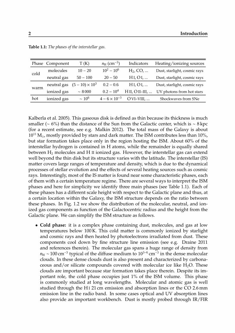
Table 1.1: The phases of the interstellar gas.
Phase Component T (K) nH (cm−3) Indicators Heating/ionizing sources
coldmolecules 10− 20 102 − 106 H2, CO, ... Dust, starlight, cosmic rays
neutral gas 50− 100 20− 50 H I, O I, ... Dust, starlight, cosmic rays
warmneutral gas (5− 10)× 103 0.2− 0.6 H I, O I, ... Dust, starlight, cosmic rays
ionized gas ∼ 8 000 0.2− 104 H II, O II–III, ... UV photons from hot stars
hot ionized gas ∼ 106 4− 6× 10⁻³ O VI–VIII, ... Shockwaves from SNe
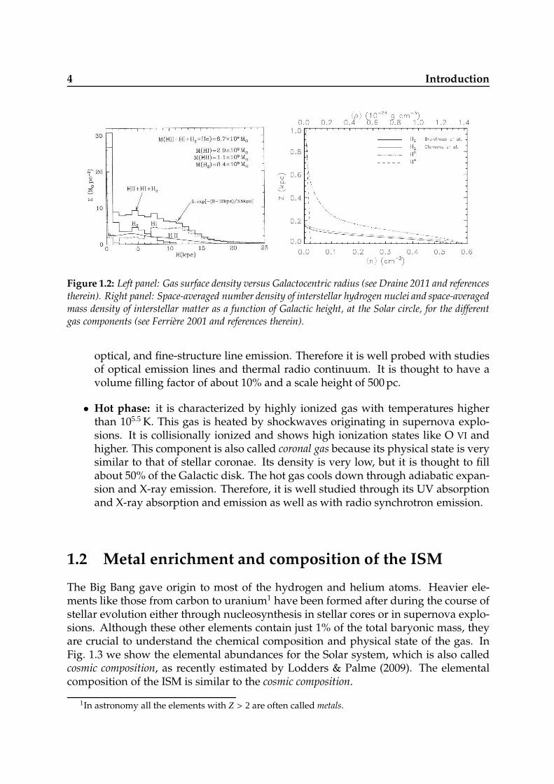
Kalberla et al. 2005). This gaseous disk is defined as thin because its thickness is muchsmaller (∼ 6%) than the distance of the Sun from the Galactic center, which is ∼ 8 kpc(for a recent estimate, see e.g. Malkin 2012). The total mass of the Galaxy is about1011 M⊙, mostly provided by stars and dark matter. The ISM contributes less than 10%,but star formation takes place only in the region hosting the ISM. About 60% of theinterstellar hydrogen is contained in H atoms, while the remainder is equally sharedbetween H2 molecules and H II ionized gas. However, the interstellar gas can extendwell beyond the thin disk but its structure varies with the latitude. The interstellar (IS)matter covers large ranges of temperature and density, which is due to the dynamicalprocesses of stellar evolution and the effects of several heating sources such as cosmicrays. Interestingly, most of the IS matter is found near some characteristic phases, eachof them with a certain temperature regime. There are several ways to interpret the ISMphases and here for simplicity we identify three main phases (see Table 1.1). Each ofthese phases has a different scale height with respect to the Galactic plane and thus, ata certain location within the Galaxy, the ISM structure depends on the ratio betweenthese phases. In Fig. 1.2 we show the distribution of the molecular, neutral, and ion-ized gas components as function of the Galactocentric radius and the height from theGalactic plane. We can simplify the ISM structure as follows.
• Cold phase: it is a complex phase containing dust, molecules, and gas at lowtemperatures below 100 K. This cold matter is commonly ionized by starlightand cosmic rays and then heated by photoelectrons irradiated from dust. Thesecomponents cool down by fine structure line emission (see e.g. Draine 2011and references therein). The molecular gas spans a huge range of density fromnH ∼ 100 cm−3 typical of the diffuse medium to 103−6 cm−3 in the dense molecularclouds. In these dense clouds dust is also present and characterized by carbona-ceous and/or silicate compounds covered with molecular ice like H2O. Theseclouds are important because star formation takes place therein. Despite its im-portant role, the cold phase occupies just 1% of the ISM volume. This phaseis commonly studied at long wavelengths. Molecular and atomic gas is wellstudied through the H I 21 cm emission and absorption lines or the CO 2.6 mmemission line in the radio band. In some cases optical and UV absorption linesalso provide an important workbench. Dust is mostly probed through IR/FIR
1.1 The multiphase structure of the ISM 3
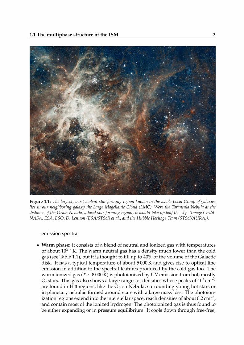
Figure 1.1: The largest, most violent star forming region known in the whole Local Group of galaxieslies in our neighboring galaxy the Large Magellanic Cloud (LMC). Were the Tarantula Nebula at thedistance of the Orion Nebula, a local star forming region, it would take up half the sky. (Image Credit:NASA, ESA, ESO, D. Lennon (ESA/STScI) et al., and the Hubble Heritage Team (STScI/AURA)).
emission spectra.
• Warm phase: it consists of a blend of neutral and ionized gas with temperaturesof about 103−4 K. The warm neutral gas has a density much lower than the coldgas (see Table 1.1), but it is thought to fill up to 40% of the volume of the Galacticdisk. It has a typical temperature of about 5 000 K and gives rise to optical lineemission in addition to the spectral features produced by the cold gas too. Thewarm ionized gas (T ∼ 8 000K) is photoionized by UV emission from hot, mostlyO, stars. This gas also shows a large ranges of densities whose peaks of 104 cm−3
are found in H II regions, like the Orion Nebula, surrounding young hot stars orin planetary nebulae formed around stars with a large mass loss. The photoion-ization regions extend into the interstellar space, reach densities of about 0.2 cm−3,and contain most of the ionized hydrogen. The photoionized gas is thus found tobe either expanding or in pressure equilibrium. It cools down through free-free,
4 Introduction
Figure 1.2: Left panel: Gas surface density versus Galactocentric radius (see Draine 2011 and referencestherein). Right panel: Space-averaged number density of interstellar hydrogen nuclei and space-averagedmass density of interstellar matter as a function of Galactic height, at the Solar circle, for the differentgas components (see Ferriere 2001 and references therein).
optical, and fine-structure line emission. Therefore it is well probed with studiesof optical emission lines and thermal radio continuum. It is thought to have avolume filling factor of about 10% and a scale height of 500 pc.
• Hot phase: it is characterized by highly ionized gas with temperatures higherthan 105.5 K. This gas is heated by shockwaves originating in supernova explo-sions. It is collisionally ionized and shows high ionization states like O VI andhigher. This component is also called coronal gas because its physical state is verysimilar to that of stellar coronae. Its density is very low, but it is thought to fillabout 50% of the Galactic disk. The hot gas cools down through adiabatic expan-sion and X-ray emission. Therefore, it is well studied through its UV absorptionand X-ray absorption and emission as well as with radio synchrotron emission.
1.2 Metal enrichment and composition of the ISM
The Big Bang gave origin to most of the hydrogen and helium atoms. Heavier ele-ments like those from carbon to uranium1 have been formed after during the course ofstellar evolution either through nucleosynthesis in stellar cores or in supernova explo-sions. Although these other elements contain just 1% of the total baryonic mass, theyare crucial to understand the chemical composition and physical state of the gas. InFig. 1.3 we show the elemental abundances for the Solar system, which is also calledcosmic composition, as recently estimated by Lodders & Palme (2009). The elementalcomposition of the ISM is similar to the cosmic composition.
1In astronomy all the elements with Z > 2 are often called metals.

1.2 Metal enrichment and composition of the ISM 5
Figure 1.3: Elemental present-day Solar system abundances as function of atomic number normalizedto 106 Si atoms (Lodders & Palme 2009).
Absorption and emission lines produced by different ionization states of metals pro-vide the temperatures, velocities, and other important physical parameters. Moreoverthe ratios between the column densities of interstellar metals and that of hydrogen, alsoknown as absolute abundances, directly yields the contribution of the stellar evolutionto the metal enrichment of the ISM. The heavy elements such as oxygen (the mostabundant one) and iron are produced in high-mass stars. Nitrogen atoms, moleculesand dust compounds are mainly formed in AGB stars and then grow in the diffuse ISM(see e.g. Mattsson & Andersen 2012). The asymptotic giant branch (AGB) is the regionof the Hertzsprung-Russell diagram characterized by evolved low to medium-mass(0.6-10 solar masses) stars. Elements heavier than Si, such as Ca, Fe, and Ni, are mostlyprovided by supernova type Ia (SN Ia). A SN Ia is a sub-category of supernovae thatresults from the violent explosion of a white dwarf star. A white dwarf is the remnantof a star that has completed its normal life cycle and has ceased nuclear fusion. If awhite dwarf gradually accretes mass from a binary companion, the general hypothesisis that its core will reach the ignition temperature for carbon fusion as it approaches thelimit. Within a few seconds after initiation of nuclear fusion, a substantial fraction ofthe matter in the white dwarf undergoes a runaway reaction, releasing enough energyto unbind the star in a supernova explosion. A Type II supernova (SN II, also known as
6 Introduction
core-collapse supernova) results from the rapid collapse and violent explosion of a mas-sive star. A star must have at least 8 times, and no more than 40− 50 times the mass ofthe Sun for this type of explosion. It is distinguished from other types of supernovaeby the presence of hydrogen in its spectrum. SN II provide most of the interstellar oxy-gen and neon. Therefore, it is clear that heavy elements directly witness the history ofthe past stellar evolution.
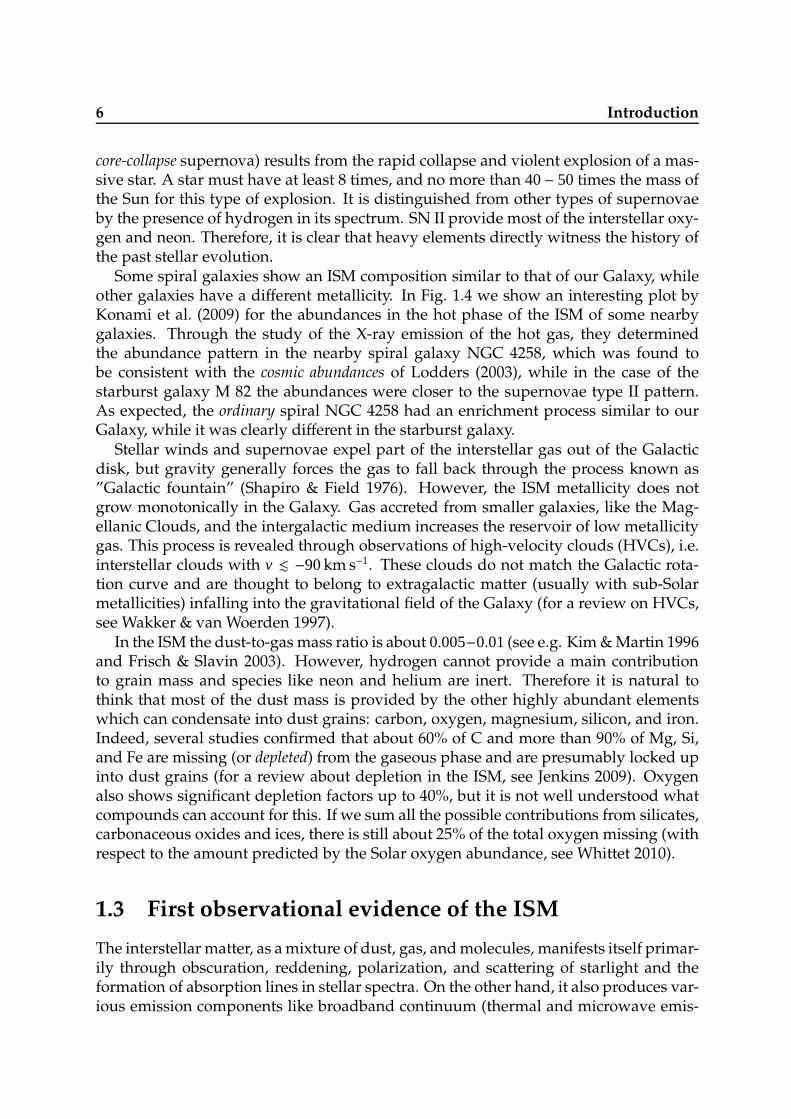
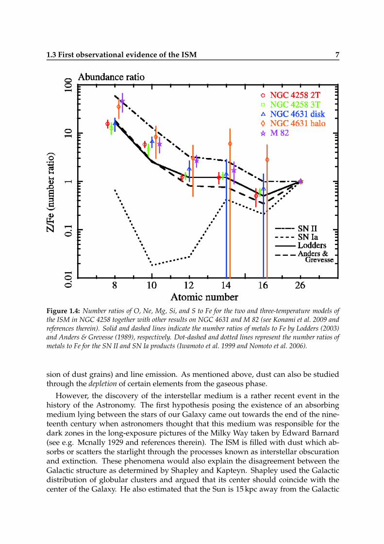
Some spiral galaxies show an ISM composition similar to that of our Galaxy, whileother galaxies have a different metallicity. In Fig. 1.4 we show an interesting plot byKonami et al. (2009) for the abundances in the hot phase of the ISM of some nearbygalaxies. Through the study of the X-ray emission of the hot gas, they determinedthe abundance pattern in the nearby spiral galaxy NGC 4258, which was found tobe consistent with the cosmic abundances of Lodders (2003), while in the case of thestarburst galaxy M 82 the abundances were closer to the supernovae type II pattern.As expected, the ordinary spiral NGC 4258 had an enrichment process similar to ourGalaxy, while it was clearly different in the starburst galaxy.
Stellar winds and supernovae expel part of the interstellar gas out of the Galacticdisk, but gravity generally forces the gas to fall back through the process known as”Galactic fountain” (Shapiro & Field 1976). However, the ISM metallicity does notgrow monotonically in the Galaxy. Gas accreted from smaller galaxies, like the Mag-ellanic Clouds, and the intergalactic medium increases the reservoir of low metallicitygas. This process is revealed through observations of high-velocity clouds (HVCs), i.e.interstellar clouds with v . −90km s−1. These clouds do not match the Galactic rota-tion curve and are thought to belong to extragalactic matter (usually with sub-Solarmetallicities) infalling into the gravitational field of the Galaxy (for a review on HVCs,see Wakker & van Woerden 1997).
In the ISM the dust-to-gas mass ratio is about 0.005−0.01(see e.g. Kim & Martin 1996and Frisch & Slavin 2003). However, hydrogen cannot provide a main contributionto grain mass and species like neon and helium are inert. Therefore it is natural tothink that most of the dust mass is provided by the other highly abundant elementswhich can condensate into dust grains: carbon, oxygen, magnesium, silicon, and iron.Indeed, several studies confirmed that about 60% of C and more than 90% of Mg, Si,and Fe are missing (or depleted) from the gaseous phase and are presumably locked upinto dust grains (for a review about depletion in the ISM, see Jenkins 2009). Oxygenalso shows significant depletion factors up to 40%, but it is not well understood whatcompounds can account for this. If we sum all the possible contributions from silicates,carbonaceous oxides and ices, there is still about 25% of the total oxygen missing (withrespect to the amount predicted by the Solar oxygen abundance, see Whittet 2010).
1.3 First observational evidence of the ISM
The interstellar matter, as a mixture of dust, gas, and molecules, manifests itself primar-ily through obscuration, reddening, polarization, and scattering of starlight and theformation of absorption lines in stellar spectra. On the other hand, it also produces var-ious emission components like broadband continuum (thermal and microwave emis-
1.3 First observational evidence of the ISM 7
Figure 1.4: Number ratios of O, Ne, Mg, Si, and S to Fe for the two and three-temperature models ofthe ISM in NGC 4258 together with other results on NGC 4631 and M 82 (see Konami et al. 2009 andreferences therein). Solid and dashed lines indicate the number ratios of metals to Fe by Lodders (2003)and Anders & Grevesse (1989), respectively. Dot-dashed and dotted lines represent the number ratios ofmetals to Fe for the SN II and SN Ia products (Iwamoto et al. 1999 and Nomoto et al. 2006).
sion of dust grains) and line emission. As mentioned above, dust can also be studiedthrough the depletion of certain elements from the gaseous phase.
However, the discovery of the interstellar medium is a rather recent event in thehistory of the Astronomy. The first hypothesis posing the existence of an absorbingmedium lying between the stars of our Galaxy came out towards the end of the nine-teenth century when astronomers thought that this medium was responsible for thedark zones in the long-exposure pictures of the Milky Way taken by Edward Barnard(see e.g. Mcnally 1929 and references therein). The ISM is filled with dust which ab-sorbs or scatters the starlight through the processes known as interstellar obscurationand extinction. These phenomena would also explain the disagreement between theGalactic structure as determined by Shapley and Kapteyn. Shapley used the Galacticdistribution of globular clusters and argued that its center should coincide with thecenter of the Galaxy. He also estimated that the Sun is 15 kpc away from the Galactic
8 Introduction
center, which is a factor of 2 higher than what we currently know (see Sect. 1.1). Her-schel and Kapteyn used the distribution of stars across the sky assuming that they havethe same intrinsic brightness and that the interstellar space was transparent to starlight(both assumptions were wrong). Therefore, they estimated that the Galaxy was about1 kpc large and thus much smaller than the current estimates (rdisk ∼ 25− 30kpc), andthat the Sun was located near the Galactic center. The presence of obscuring inter-stellar matter gave Herschel and Kapteyn the false impression that the spatial densitydecreases isotropically in any direction away from us and brought them to misplace theSun near the center of the Galaxy. Shapley did not encounter the same problem withglobular clusters, because they are intrinsically much brighter and easier to recognizethan individual stars and because most of them lie outside the thin layer of obscuringmaterial.
The first direct evidence of the ISM was the discovery of stable Ca II absorption linesin the spectrum of the spectroscopic binary δ Orionis (Hartmann 1904). Lines intrin-sic to the binary systems are generally variable and Doppler-shifted. Trumpler (1930)first discovered that the reddening of stars of a certain spectral type (i.e. the absorp-tion of the blue / short wavelengths) increases with the distance, which brought theidea that the interstellar space contains dust that produces absorption and extinction.Strong evidence of the interstellar medium and spatial distribution of interstellar H I
was obtained in the second half of the twentieth century through observations withradio telescopes (see e.g. Binney & Merrifield 1998 chapter 10 and references therein).These observations showed that the interstellar H I follows a spiral structure similar tothat observed in external galaxies. The Sun was indeed far away from the center of thespiral arms but at a two times smaller distance than that predicted by Shapley.
1.4 X-ray spectroscopy of the ISM
In X-rays the ISM produces several emission or absorption phenomena, neverthelessX-ray astrophysics of the ISM is a very young science, whose development startedwith the discovery of the ISM hot phase. Spitzer (1956) predicted the existence of a hotcoronal phase in the ISM, which was required to provide sufficient pressure to confineobserved high-altitude clouds. However, only in the seventies the first evidence ofthe hot gas was revealed in the UV energy domain with the Copernicus satellite (York1974) and in X-rays with rocket missions (Williamson et al. 1974). The analysis of thesoft X-ray background at 0.25 keV indicated that most of the emitting gas was locatedwithin the Local Bubble with temperatures of about 106 K (see Cox & Reynolds 1987and McCammon & Sanders 1990a). Important improvements in the study of the emis-sion of the hot gas were provided by the launch of the ROSAT satellite (see Fig. 1.5),which brought discovery of emission from regions outside the Local Bubble and evenfrom extragalactic space (Snowden et al. 1998). The launch of new X-ray missions likeChandra, XMM-Newton, and Suzaku improved the study of the ISM. However, X-rayemission lines are suitable only for determining the physics and chemistry of the hotphase of the ISM either in the Milky Way (see e.g. Hagihara et al. 2011) or in externalgalaxies such as M 31 (Liu et al. 2010) and NGC 4258 (Konami et al. 2009).
1.4 X-ray spectroscopy of the ISM 9
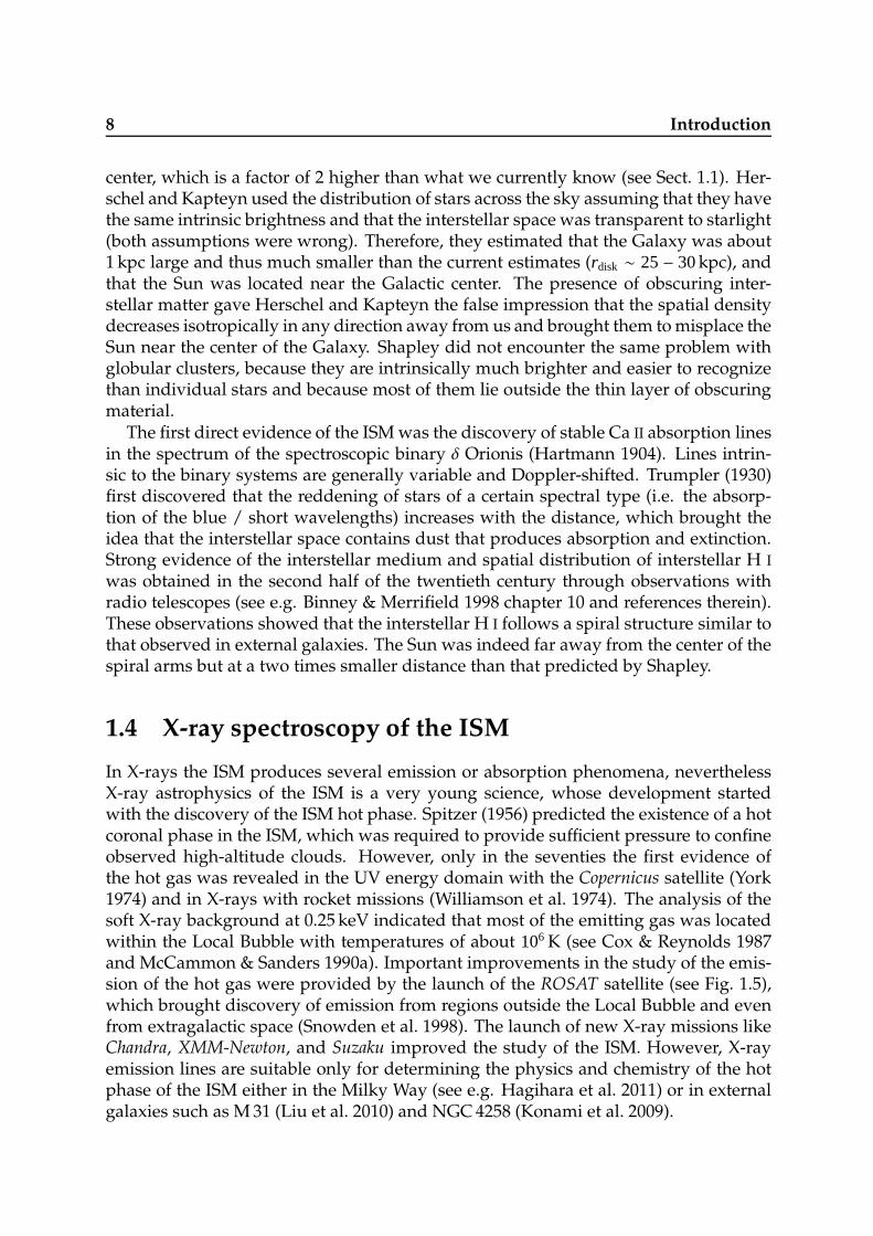
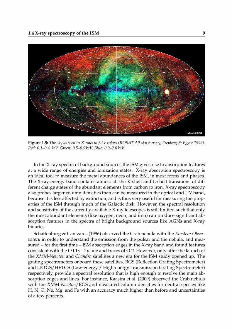
Figure 1.5: The sky as seen in X-rays in false colors (ROSAT All-sky Survey, Freyberg & Egger 1999).Red: 0.1–0.4 keV. Green: 0.5–0.9 keV. Blue: 0.9–2.0 keV.
In the X-ray spectra of background sources the ISM gives rise to absorption featuresat a wide range of energies and ionization states. X-ray absorption spectroscopy isan ideal tool to measure the metal abundances of the ISM, in most forms and phases.The X-ray energy band contains almost all the K-shell and L-shell transitions of dif-ferent charge states of the abundant elements from carbon to iron. X-ray spectroscopyalso probes larger column densities than can be measured in the optical and UV band,because it is less affected by extinction, and is thus very useful for measuring the prop-erties of the ISM through much of the Galactic disk. However, the spectral resolutionand sensitivity of the currently available X-ray telescopes is still limited such that onlythe most abundant elements (like oxygen, neon, and iron) can produce significant ab-sorption features in the spectra of bright background sources like AGNs and X-raybinaries.
Schattenburg & Canizares (1986) observed the Crab nebula with the Einstein Obser-vatory in order to understand the emission from the pulsar and the nebula, and mea-sured – for the first time – ISM absorption edges in the X-ray band and found featuresconsistent with the O I 1s− 2p line and traces of O II. However, only after the launch ofthe XMM-Newton and Chandra satellites a new era for the ISM study opened up. Thegrating spectrometers onboard these satellites, RGS (Reflection Grating Spectrometer)and LETGS/HETGS (Low-energy / High-energy Transmission Grating Spectrometer)respectively, provide a spectral resolution that is high enough to resolve the main ab-sorption edges and lines. For instance, Kaastra et al. (2009) observed the Crab nebulawith the XMM-Newton/RGS and measured column densities for neutral species likeH, N, O, Ne, Mg, and Fe with an accuracy much higher than before and uncertaintiesof a few percents.
10 Introduction
Some years before, Paerels et al. (2001) observed the low-mass X-ray binary (LMXB)4U 0614+091 with the aim of probing emission lines intrinsic to the source, which werediscovered a few years before. They did not find any of those lines, but detect K-shellabsorption by interstellar O and Ne, and L-shell absorption by Fe. From this momentit became clear that X-ray spectroscopy has indeed the power to probe the ISM. A firstdedicated study on the ISM was carried by Juett et al. (2004). They observed a smallsample of X-ray binaries with the HETGS onboard Chandra and measured column den-sities of neutral, singly and doubly ionized oxygen. They constrained some ionizationratios for the interstellar gas: O II / O I ∼ 0.1 and O III / O I . 0.1. They also estimatedthe velocity dispersion of the neutral lines to be . 200km s−1, which suggests that theabsorption lines originate in the ISM rather than in a circumstellar environment localto the binaries. A couple of years later, Juett et al. (2006) extended the analysis to the Neand Fe edges and measured interesting abundance ratios: O/Ne = 5.4±1.6 and Fe/Ne= 0.20± 0.03. The first was consistent with the standard ISM abundances (Wilms et al.2000), while the latter was significantly lower. They attributed this difference to irondepletion into dust grains in the interstellar medium. They also measured large de-grees of ionization: Ne II / Ne I ∼ 0.3 and Ne III / Ne I ∼ 0.07. This was just the preludeto a big series of discoveries.
Yao & Wang (2005) systematically studied the hot gas towards a sample of 12 sour-ces, mostly LMXBs, and obtained a typical temperature of about 2× 10⁶ K and a scale-height of about 1 kpc. Yao & Wang (2006) first constrained the multiphase structureof the ISM through high-resolution X-ray spectroscopy of the cold, warm, and hotphases. They measured column densities of oxygen on a broad range of ionizationstates as well as oxygen abundances (by comparing their oxygen column densities withthe hydrogen measurements at 21 cm). The cold and warm gas respectively providedO/H = 0.2 − 0.6 and 1.1 − 3.5 (in units of Solar abundances, see Anders & Grevesse1989), which was interpreted as a result of molecule/dust grain destruction and recentmetal enrichment in the warm ionized and hot phases. Recently, Yao et al. (2009a)found high-ionization absorption lines of ions such as O VI to O VIII and Ne VIII to Ne X
in the HETGS spectrum of the low-mass X-ray binary Cyg X-2, and argued that thebulk of the O VI should originate from the conductive interface between the cool andthe hot gas in accordance with Richter (2006).
Other work has revealed a complex structure around the oxygen K-shell absorptionedge (de Vries et al. 2003). Lee & Ravel (2005) proposed to use the iron absorptionedges for determining quantity and composition of interstellar dust. This was suc-cessfully applied to Chandra/HETGS observations of the X-ray binary Cygnus X-1 byLee et al. (2009), who found evidence for hematite and iron silicates. More work oninterstellar dust followed. Costantini et al. (2005) argued that the feature near the O I
K-edge of the scattering halo of Cyg X-2 can be attributed to dust towards the source,with a major contribution from silicates such as olivine and pyroxene. In their paperon Sco X-1, observed with XMM-Newton, de Vries & Costantini (2009) found clear indi-cations of extended X-ray absorption fine structures (EXAFS) maybe due to dust nearthe absorption edge of oxygen. Costantini et al. (2012) combined Chandra and XMM-Newton spectra of the bright LMXB 4U 1820-303 and found the dust to provide about20% of oxygen and 90% of iron. They also suggested a major contribution of Mg-rich

1.5 Thesis aims and structure 11
silicates, with metallic iron inclusion, and a composition similar to the well studieddust constituent (GEMS), sometimes proposed as a silicate constituent in our Galaxy.
The current X-ray satellites will be operating for most of this decade and a new X-ray mission (ASTRO–H, Takahashi et al. 2010) will be launched in two years from now.The soft X-ray Calorimeter Spectrometer (SXS) onboard this satellite will provide forthe first time a high spectral resolution in the broad 0.3−12keV energy band combinedwith high sensitivity and the possibility of a simultaneous analysis of the Fe K and Ledges as well as high quality Mg and Si absorption spectra. Lee et al. (2009) showedthat it is indeed possible to differentiate dust constituents with the SXS.
1.5 Thesis aims and structure
It is clear that high-resolution X-ray spectroscopy provides an important workbenchfor the study of the ISM and it is worth to say that we are in the golden age of the ISM X-ray spectroscopy. The current and future X-ray satellites provide accurate estimates ofinterstellar column densities, ionization states, and depletion factors, which are usefulto determine the chemical and physical state of all the phases of the ISM. However, asystematic study on this field is yet to be done and there are several open questionson the ISM. What is the exact molecular structure of the cold interstellar phase? What arethe depletion factors? Is any phase in a certain equilibrium state and which one? What arethe total elemental abundances? How do all these parameters relate to the specific Galacticenvironment? How do the abundances vary in the Galaxy and how are they correlated with themetal enrichment provided by AGB stars, supernovae and other sources?
This thesis aims to find and provide a solution to some of these problems. In partic-ular we focus on the study of the ISM through high-resolution X-ray spectroscopy ofbright background sources. The analysis of its absorption lines provides us with accu-rate measurements of column densities and abundances for several elemental species.This allows us to determine the multiphase structure and the chemical compositionof the ISM. We also measure the metallicity gradient of the ISM in the Galaxy whichdepends on the stellar elemental yields, and it is thus linked to the evolution of theGalaxy.
• In Chapter 2 we show a simple approach to determine the multiphase structureof the ISM through the observation of its absorption lines and edges in the high-quality X-ray spectrum of the LMXB GS 1826−238. We provide an unprecedent-edly detailed treatment of the absorption features caused by the dust and boththe neutral and ionized gas of the ISM. We constrain the column density ratioswithin the different phases of the ISM and measure the abundances of elementssuch as O, Ne, Fe, and Mg. There are significant deviations from the proto-Solarabundances, which are consistent with the Galactic metallicity gradient: the ISMappears to be metal-rich in the inner regions. Up to about 10% of the gas is ion-ized. Signatures of dust and molecules are also clearly detected: they account formost iron and between 10 and 40% of oxygen.
12 Introduction
• The metal enrichment in the ISM is a product of stellar evolution, but each typeof star releases a certain amount of metals in the surrounding space dependingon the detailed nucleosynthesis. Novae are a subclass of cataclysmic variablesconsisting of a white dwarf (WD) that accretes gas (mostly hydrogen) from acompanion star. When the accretion of matter surpasses a certain limit then hy-drogen in the WD outer layer starts to burn into helium and pulls out matter fromthe WD into the surrounding medium, which is enriched by metals and dust. InChapter 3 we show that the deep absorption lines of the X-ray spectrum of novaV2491 Cyg are well described by a phenomenological model consisting of threehighly ionized expanding shells. Rest-frame absorption lines are produced bycold circumstellar and interstellar matter that includes dust. The abundances ofthe shells indicate that they were ejected from an O-Ne white dwarf. High abun-dances of O and N in the cold absorbing gas shows that the surrounding mediumis significantly enriched of metals by the nova ejecta.
• The ISM structure varies with the Galactic altitude. Near the Galactic plane mostof the matter is stored in cold gas and dust, while at higher altitudes the ionizedgas has a predominant role. AGNs are optimal background sources for the anal-ysis of the ISM in the disk and halo of the Galaxy as several of them are brightand have column densities high enough to show strong interstellar absorptionfeatures. In Chapter 4 we use high-quality X-ray and UV spectra of AGN Mrk509, located at intermediate-high Galactic latitudes obtained with XMM-Newton,HST and FUSE. We use advanced absorption models consisting of photo- andcollisional-ionization in order to constrain the column density ratios of the differ-ent phases of the interstellar medium (ISM) and measure the abundances of C,N, O, Ne, Mg, Al, Si, S, and Fe. The high-resolution UV spectra allow to differen-tiate between up to seven velocity components, which belong to different kindsof interstellar clouds. We determine their origin and location within the Galacticenvironment.
• In Chapter 5 we show a simple method to probe the ISM dust composition, to-tal abundances, and abundance gradients through the study of interstellar ab-sorption features in the high-quality spectra of nine LMXBs taken with XMM-Newton. We measure the column densities of O, Ne, Mg, and Fe with an em-pirical model and estimate the Galactic abundance gradients. We find that solidoxygen is mostly provided by ices and silicates. 15–20% and 70–90% of the totalamount of O I and Fe I is found in dust, respectively. The amount and composi-tion of dust seems to be consistent along all lines-of-sight (LOS). On a large scalethe ISM appears to be chemically homogeneous showing similar gas ionizationratios and dust mixtures. The agreement between the abundances of the ISM andthe stellar objects suggests that the local Galaxy is also chemically homogeneous.
Chapter 2
High-resolution X-ray spectroscopy ofthe Interstellar Medium
C. Pinto1, J. S. Kaastra1,2, E. Costantini1, F. Verbunt2
1 SRON Netherlands Institute for Space Research, Utrecht, The Netherlands2 Astronomical Institute, Utrecht University, Utrecht, The Netherlands
Received 21 April 2010 / Accepted 13 July 2010
Published in Astronomy & Astrophysics, volume 521, pages A79–89, 2010
Abstract
The interstellar medium (ISM) has a multiphase structure characterized by gas, dust,and molecules. The gas can be found in different charge states: neutral, weakly ion-ized (warm) and highly ionized (hot). It is possible to probe the multiphase ISMthrough the observation of its absorption lines and edges in the X-ray spectra of back-ground sources. We present a high-quality RGS spectrum of the low-mass X-ray binaryGS 1826−238 with an unprecedentedly detailed treatment of the absorption featurescaused by the dust and both the neutral and ionized gas of the ISM. We constrain thecolumn density ratios within the different phases of the ISM and measure the abun-dances of elements such as O, Ne, Fe, and Mg. We found significant deviations fromthe protosolar abundances: oxygen is over-abundant by a factor 1.23± 0.05, neon by1.75± 0.11, iron by 1.37± 0.17, and magnesium by 2.45± 0.35. The abundances are
14 High-resolution X-ray spectroscopy of the Interstellar Medium
consistent with the measured metallicity gradient in our Galaxy: the ISM appears tobe metal-rich in the inner regions. The spectrum also shows the presence of warm andhot ionized gas. The gas column has a total ionization degree of less than 10%. We alsoshow that dust plays an important role as expected from the position of GS 1826−238:most iron appears to be bound in dust grains, while 10−40% of oxygen consist of amixture of dust and molecules.
2.1 Introduction
The interstellar medium of our Galaxy (ISM) is a mixture of dust and gas in the form ofatoms, molecules, ions, and electrons. It manifests itself primarily through obscuration,reddening and polarization of starlight and the formation of absorption lines in stellarspectra, and secondly through various emission mechanisms (broadband continuumand line emission). The gas is found in both neutral and ionized phases (for a review,see Ferriere 2001). The neutral phase is a blend of cold molecular gas (T ∼ 20− 50K),found in the so-called dark clouds, and cold atomic gas (T ∼ 100K) inherent in thediffuse clouds, while the warm atomic gas has temperatures of up to 104 K. The atomicgas is well traced by H I and mainly concentrated in the Galactic plane with clouds upto few hundreds pc above it. The warm ionized gas is a weakly ionized gas, with atemperature of ∼ 104 K. It is mainly traced by Hα-line emission and pulsar dispersionmeasures; it can reach a vertical height of 1 kpc. The hot ionized gas is characterized bytemperatures of about 106 K. It is heated by supernovae and stellar winds from massivestars; it gives rise to high-ionization absorption lines and the soft X-ray backgroundemission. The study of the ISM is very interesting because of its connection with theevolution of the entire Galaxy: the stellar evolution enriches the interstellar mediumwith heavy elements, while the ISM acts as a source of matter for the star-formingregions.
High-resolution X-ray spectroscopy has become a powerful diagnostic tool for con-straining the chemical and physical properties of the ISM. Through the study of theX-ray absorption lines in the spectra of background sources it is possible to probe thevarious phases of the ISM of the Galaxy. First of all, the K-shell transitions of low-Zelements, such as oxygen and neon, and the L-shell transitions of iron fall inside thesoft X-ray energy band. Secondly, the different charge states for each element allow usto constrain the multiphase ISM, e.g. its ionization state and temperature distribution.
Schattenburg & Canizares (1986) first measured ISM absorption edges in the X-rayband with the Einstein Observatory and found features consistent with the O I 1s − 2pline and traces of O II. After the launch of the XMM-Newton and Chandra satellitesa new era for the ISM study opened up. The grating spectrometers onboard thesesatellites, RGS and LETGS/HETGS respectively, provide a spectral resolution that ishigh enough to resolve the main absorption edges and lines. Recently, Yao et al. (2009a)found high-ionization absorption lines of ions such as O VI to O VIII and Ne VIII to Ne X
in the HETGS spectrum of the low-mass X-ray binary Cyg X-2, and argued that thebulk of the O VI should originate from the conductive interface between the cool andthe hot gas. Other work has revealed a complex structure around the oxygen K-shell
2.2 Observations and data reduction 15
Table 2.1: Observations used in this paper. We report the total exposure length together with the netexposure time remaining after screening of the background and removal of bursts.
ID Date Length RGS PN(ks) (ks) (ks)
0150390101 2003 April 6 108 67.8 63.80150390301 2003 April 8 92 77.8 67.8
absorption edge (Paerels et al. 2001; de Vries et al. 2003; Juett et al. 2004). Costantiniet al. (2005) argued that the feature of the scattering halo of Cyg X-2 near the O I K-edgecan be attributed to dust towards the source, with a major contribution from silicatessuch as olivine and pyroxene. In their paper on Sco X-1, observed with XMM-Newton,de Vries & Costantini (2009) found clear indications of extended X-ray absorption finestructures (EXAFS) near the absorption edge of oxygen.
In this work we report the detection of absorption lines and edges in the high-qualityspectrum of the low-mass X-ray binary (LMXB) GS 1826−238 obtained with the XMM-Newton Reflection Grating Spectrometer (RGS, den Herder et al. 2001). In order to con-strain the continuum parameters we also used the EPIC-pn (Struder et al. 2001) datasetof this source. Thompson et al. (2008), using the XMM-Newton and RXTE observationsof April 2003, derived a high unabsorbed bolometric flux F ∼ 3.5 × 10⁻¹² W m−2. Thesource is well suited for the analysis of the ISM also because of its column densityNH ∼ 4×1025 m−2 (see Table 2.3), which is sufficiently high to produce prominent O andFe edges. We assume the distance of the source to be 6.1± 0.2kpc (Heger et al. 2007).
We analyze the absorption in the spectrum as follows. We first remove the bursts,because they add a strongly variable component to the spectrum. Then we determinethe source continuum by simultaneously fitting EPIC and RGS data. In a second in-stance we use only the high-resolution RGS spectra to constrain the absorption contri-butions. We search for statistically significant features by adding several absorbers insequence: cold gas, warm gas, hot gas, dust, and molecules. All of these appear to beimportant.
2.2 Observations and data reduction
The source GS 1826−238 (Galactic coordinates l = 9.27, b = −6.09) has been observedtwice with XMM-Newton for a total length of 200 ks (see Table 5.1 for details). The dataare reduced with the XMM-Newton Science Analysis System (SAS) version 9.0.1.
GS 1826−238 is a bursting LMXB with a regular time separation between the bursts.Because the primary aim of the XMM-Newton observations was the study of the bursts,the EPIC-pn detector was operated in timing mode, which means that imaging is madeonly in one dimension, along the RAWX axis. Along the row direction (RAWY axis),data from a predefined area on one CCD chip are collapsed into a one-dimensional rowfor a fast read-out. Then source photons are extracted between RAWX values 30− 45and background photons are extracted between rows 2 − 16, as recommended by thestandard procedure.
16 High-resolution X-ray spectroscopy of the Interstellar Medium
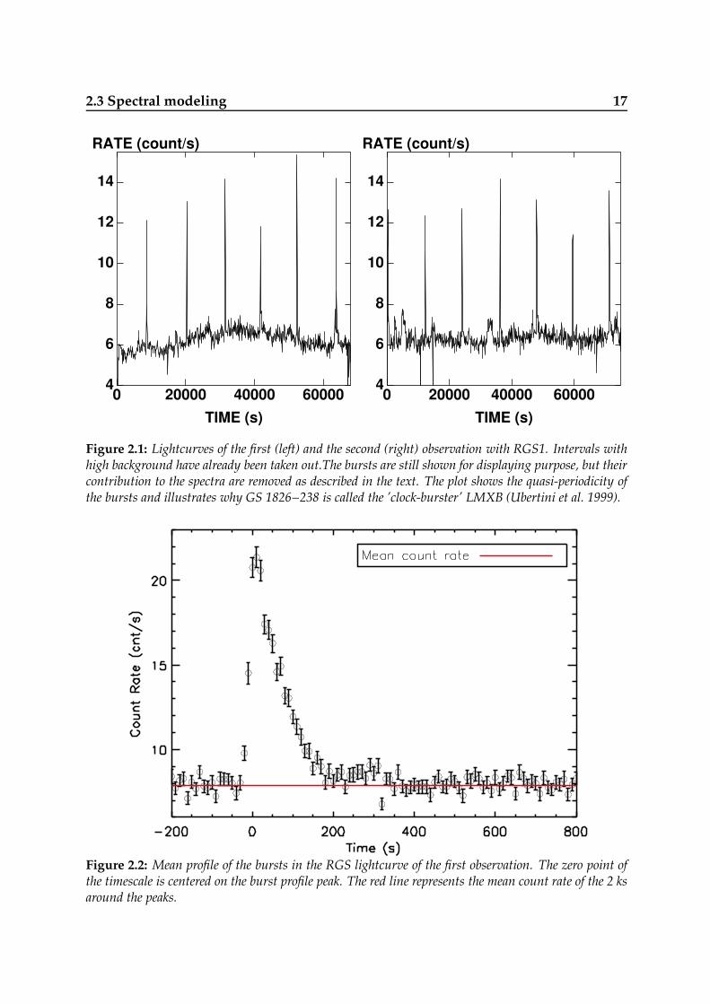
We produced pn lightcurves mainly to remove the burst intervals and to extract thespectra of the persistent part of the lightcurve. In the first observation nine bursts wedetected, in the second observation seven bursts. We plot the burst profiles of these 16bursts in Fig. 2.2. We estimate a mean duration of about 300 s for the bursts, and weremoved for each burst 50 s before the peak to 250 s after it. Recently in’t Zand et al.(2009) suggested a mean duration of about 1 ks for the bursts, but they also arguedthat after the first 100 s the inferred emission decreases sharply by at least one order ofmagnitude, contributing only about 3% to the fluence in the burst. After 250 s the fluxof the burst has decreased by almost two orders of magnitude and its profile mergeswith the persistent lightcurve. Thus, by removing 300 s for each burst, we retain lessthan ∼ 1% burst emission, which is negligible compared to the persistent emission.
We processed the RGS data with the SAS task rgsproc. We produced the lightcurvesfor the background in CCD9 following the XMM-SAS guide1 in order to remove softproton flares and spurious events. We created good time intervals (GTI) by removingintervals with count rates higher than 0.5 c s−1. We reprocessed the data again withrgsproc by filtering them with the GTI for background screening and bursts removal.We extracted response matrices and spectra for the two observations. The final netexposure times are reported in Table 5.1.
Our analysis focuses on the 7 − 31 Å (0.4 − 1.77 keV) first order spectra of the RGSdetector. In order to fit the spectral continuum properly, we also use the 0.5− 10 keVEPIC spectra of both observations. We performed the spectral analysis with SPEX2
version 2.01.05 (Kaastra et al. 1996). We scaled the elemental abundances to the pro-tosolar abundances of Lodders (2003): N/H = 7.943×10⁻⁵, O/H = 5.754×10⁻⁴, Ne/H =8.912×10⁻⁵, Mg/H = 4.169×10⁻⁵, Fe/H = 3.467×10⁻⁵. We use the C-statistic throughoutthe paper and adopt 1σ errors.
2.3 Spectral modeling
The first step of the spectral analysis consists of the determination of the continuumemission and the dominant absorption component. The best way to do this is to fitthe spectra of RGS and EPIC-pn simultaneously. The XMM-Newton cross-calibrationis very complex, not only because of the different energy bands, but mainly because oftheir different features: RGS is sensitive in the soft X-ray energies with high spectralresolution, showing narrow absorption features, while pn has a low spectral resolution,therefore blurring the absorption features seen with RGS. EPIC-pn has a higher countrate compared to RGS and a broader energy band. The original RGS spectra are binnedby a factor of 10 in this simultaneous fit. This is necessary to temporarily remove thenarrow features due to the absorption lines. The pn spectra are resampled in bins ofabout 1/3 of the spectral resolution (FWHM ∼ 50−150 eV between 0.5−10 keV), whichis the optimal binning for most spectra.
A better local fit for absorption edges and lines is obtained from a separate RGS fit.In the RGS local fit we rebin the spectra only by a factor of two, i.e. about 1/3 FWHM
1http://heasarc.nasa.gov/docs/xmm/abc/2www.sron.nl/spex
2.3 Spectral modeling 17
0 20000 40000 600004
6
8
10
12
14
TIME (s)
RATE (count/s)
0 20000 40000 600004
6
8
10
12
14
TIME (s)
RATE (count/s)
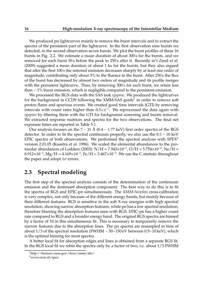
Figure 2.1: Lightcurves of the first (left) and the second (right) observation with RGS1. Intervals withhigh background have already been taken out.The bursts are still shown for displaying purpose, but theircontribution to the spectra are removed as described in the text. The plot shows the quasi-periodicity ofthe bursts and illustrates why GS 1826−238 is called the ’clock-burster’ LMXB (Ubertini et al. 1999).
Figure 2.2: Mean profile of the bursts in the RGS lightcurve of the first observation. The zero point ofthe timescale is centered on the burst profile peak. The red line represents the mean count rate of the 2 ksaround the peaks.
18 High-resolution X-ray spectroscopy of the Interstellar Medium
(the first order RGS spectra provide a resolution of 0.06−0.07 Å). This gives at least 10counts/bin and a bin size of about 0.02 Å.
2.3.1 Simultaneous EPIC−RGS fits
At first we followed the spectral modeling of Thompson et al. (2008). The continuumspectrum is modeled by emission from a blackbody and two comptonization mod-els. The blackbody component arises from the thermal emission of the accretion diskaround the neutron star. The first comptonization component (hereafter C1) describesthe energy gain of the disk soft photons by scattering in the accretion disk corona. Thesecond comptonization component C2 corresponds to scattered seed photons originat-ing from regions closer to the NS surface, i.e. the boundary layer. Thompson et al.(2008) applied a neutral absorber to the continuum mentioned above and fitted XMM-Newton, Chandra, and RXTE data. For this purpose we used the absm model in SPEX:the model calculates the continuum transmission of neutral gas with cosmic abun-dances as published by Morrison & McCammon (1983). In our case the same modeldoes not give a satisfactory fit, especially around the neon and oxygen edges, and can-not fit the O I line. This could be expected because the Morrison & McCammon (1983)model does not take into account the absorption lines and the possible variations in theabundances. Therefore we replace the absm component with a hot component, whichdescribes the transmission through a layer of collisionally ionized plasma. At low tem-peratures it calculates the absorption of (almost) neutral gas (for further informationsee the SPEX manual). We left the temperature and the O, Ne, Mg, and Fe abundancesof this absorber free in the fit. In the fits we ignored two small regions (17.2 − 17.7 Åand 22.7 − 23.2 Å), close to the iron and oxygen edges respectively. The presence ofdust and molecules affects the fine structure of the edge, thus these regions will beanalyzed with more complex models in Sect. 2.3.2. However, the ISM abundanceswere determined by the depth of the absorption edges, thus ignoring these small re-gions we could still constrain the abundances of these elements (Kaastra et al. 2009).Indeed, in Sect. 5.5.4 and Table 2.6 we will validate this assumption. We obtained agood fit with C-stat/dof 3
= 2451/1705and 2579/1710in the two observations (see Fig.2.3). The parameters for both observations are listed in Table 4.1. We call this simplemodel, where the ISM is modeled with one (neutral) gas component, Model A. Theabundances mostly agree between the two observations, but they are not reliable. InSects. 4.4.2 and 5.5.4 we show that the RGS fit provides a column density higher by10%, which significantly changes the abundance estimates. There are also small dif-ferences in the continuum parameters, such as the electron temperatures. Indeed wefind different temperatures for both comptonization components (see Table 4.1). Thesesmall deviations affect the broadband spectral slope and forbid to fit the two EPIC-pnobservations simultaneously, while this is possible with the RGS spectra.
We also tested alternative continuum models in order to show that the adoptedmodel is the best one. Thompson et al. (2008) showed that the spectral modeling ofGS 1826−238 can be done with other continuum models: 1) blackbody emission plus
3Here and hereafter dof means degrees of freedom.
2.3 Spectral modeling 19
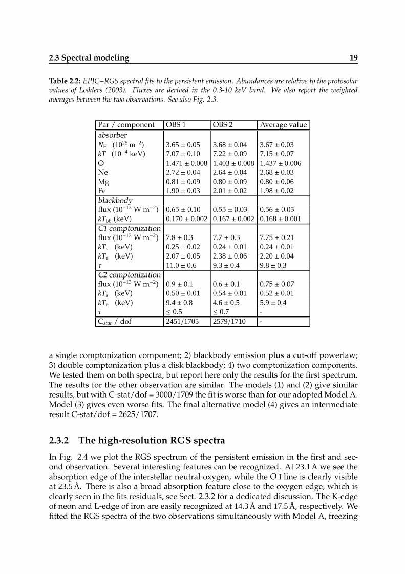
Table 2.2: EPIC−RGS spectral fits to the persistent emission. Abundances are relative to the protosolarvalues of Lodders (2003). Fluxes are derived in the 0.3-10 keV band. We also report the weightedaverages between the two observations. See also Fig. 2.3.
Par / component OBS 1 OBS 2 Average value
absorberNH (1025 m−2) 3.65± 0.05 3.68± 0.04 3.67± 0.03kT (10−4 keV) 7.07± 0.10 7.22± 0.09 7.15± 0.07O 1.471± 0.008 1.403± 0.008 1.437± 0.006Ne 2.72± 0.04 2.64± 0.04 2.68± 0.03Mg 0.81± 0.09 0.80± 0.09 0.80± 0.06Fe 1.90± 0.03 2.01± 0.02 1.98± 0.02blackbodyflux (10−13 W m−2) 0.65 ± 0.10 0.55 ± 0.03 0.56 ± 0.03kTbb (keV) 0.170± 0.002 0.167± 0.002 0.168± 0.001C1 comptonizationflux (10−13 W m−2) 7.8 ± 0.3 7.7 ± 0.3 7.75 ± 0.21kTs (keV) 0.25± 0.02 0.24± 0.01 0.24± 0.01kTe (keV) 2.07± 0.05 2.38± 0.06 2.20± 0.04τ 11.0± 0.6 9.3± 0.4 9.8± 0.3C2 comptonizationflux (10−13 W m−2) 0.9 ± 0.1 0.6 ± 0.1 0.75 ± 0.07kTs (keV) 0.50± 0.01 0.54± 0.01 0.52± 0.01kTe (keV) 9.4± 0.8 4.6± 0.5 5.9± 0.4τ ≤ 0.5 ≤ 0.7 -
Cstat / dof 2451/1705 2579/1710 -
a single comptonization component; 2) blackbody emission plus a cut-off powerlaw;3) double comptonization plus a disk blackbody; 4) two comptonization components.We tested them on both spectra, but report here only the results for the first spectrum.The results for the other observation are similar. The models (1) and (2) give similarresults, but with C-stat/dof = 3000/1709 the fit is worse than for our adopted Model A.Model (3) gives even worse fits. The final alternative model (4) gives an intermediateresult C-stat/dof = 2625/1707.
2.3.2 The high-resolution RGS spectra
In Fig. 2.4 we plot the RGS spectrum of the persistent emission in the first and sec-ond observation. Several interesting features can be recognized. At 23.1 Å we see theabsorption edge of the interstellar neutral oxygen, while the O I line is clearly visibleat 23.5 Å. There is also a broad absorption feature close to the oxygen edge, which isclearly seen in the fits residuals, see Sect. 2.3.2 for a dedicated discussion. The K-edgeof neon and L-edge of iron are easily recognized at 14.3 Å and 17.5 Å, respectively. Wefitted the RGS spectra of the two observations simultaneously with Model A, freezing
20 High-resolution X-ray spectroscopy of the Interstellar Medium
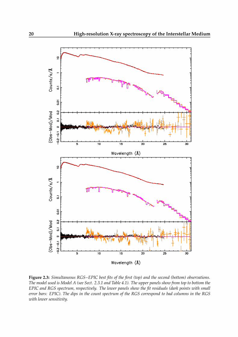
Figure 2.3: Simultaneous RGS−EPIC best fits of the first (top) and the second (bottom) observations.The model used is Model A (see Sect. 2.3.1 and Table 4.1). The upper panels show from top to bottom theEPIC and RGS spectrum, respectively. The lower panels show the fit residuals (dark points with smallerror bars: EPIC). The dips in the count spectrum of the RGS correspond to bad columns in the RGSwith lower sensitivity.
2.3 Spectral modeling 21
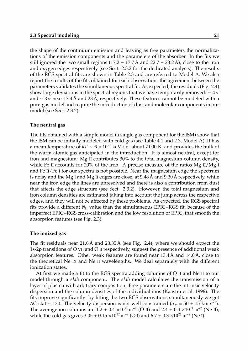
the shape of the continuum emission and leaving as free parameters the normaliza-tions of the emission components and the parameters of the absorber. In the fits westill ignored the two small regions (17.2 − 17.7 Å and 22.7 − 23.2 Å), close to the ironand oxygen edges respectively (see Sect. 2.3.2 for the dedicated analysis). The resultsof the RGS spectral fits are shown in Table 2.3 and are referred to Model A. We alsoreport the results of the fits obtained for each observation: the agreement between theparameters validates the simultaneous spectral fit. As expected, the residuals (Fig. 2.4)show large deviations in the spectral regions that we have temporarily removed: ∼ 4σand ∼ 3σ near 17.4 Å and 23 Å, respectively. These features cannot be modeled with apure-gas model and require the introduction of dust and molecular components in ourmodel (see Sect. 2.3.2).
The neutral gas
The fits obtained with a simple model (a single gas component for the ISM) show thatthe ISM can be initially modeled with cold gas (see Table 4.1 and 2.3, Model A). It hasa mean temperature of kT ∼ 6 × 10⁻⁴ keV, i.e. about 7 000 K, and provides the bulk ofthe warm atomic gas anticipated in the introduction. It is almost neutral, except foriron and magnesium: Mg II contributes 30% to the total magnesium column density,while Fe II accounts for 20% of the iron. A precise measure of the ratios Mg II/Mg I
and Fe II/Fe I for our spectra is not possible. Near the magnesium edge the spectrumis noisy and the Mg I and Mg II edges are close, at 9.48 Å and 9.30 Å respectively, whilenear the iron edge the lines are unresolved and there is also a contribution from dustthat affects the edge structure (see Sect. 2.3.2). However, the total magnesium andiron column densities are estimated taking into account the jump across the respectiveedges, and they will not be affected by these problems. As expected, the RGS spectralfits provide a different NH value than the simultaneous EPIC−RGS fit, because of theimperfect EPIC−RGS cross-calibration and the low resolution of EPIC, that smooth theabsorption features (see Fig. 2.3).
The ionized gas
The fit residuals near 21.6 Å and 23.35 Å (see Fig. 2.4), where we should expect the1s-2p transitions of O VII and O II respectively, suggest the presence of additional weakabsorption features. Other weak features are found near 13.4 Å and 14.6 Å, close tothe theoretical Ne IX and Ne II wavelengths. We deal separately with the differentionization states.
At first we made a fit to the RGS spectra adding columns of O II and Ne II to ourmodel through a slab component. The slab model calculates the transmission of alayer of plasma with arbitrary composition. Free parameters are the intrinsic velocitydispersion and the column densities of the individual ions (Kaastra et al. 1996). Thefits improve significantly: by fitting the two RGS observations simultaneously we get∆C-stat ∼ 130. The velocity dispersion is not well constrained (σV = 50 ± 15 km s−1).The average ion columns are 1.2 ± 0.4 ×10²¹ m−2 (O II) and 2.4 ± 0.4 ×10²¹ m−2 (Ne II),while the cold gas gives 3.05 ± 0.15 ×10²² m−2 (O I) and 6.7 ± 0.3 ×10²¹ m−2 (Ne I).
22 High-resolution X-ray spectroscopy of the Interstellar Medium
0
50
100
150
Pho
tons
m−
2 s−
1 Å
−1
O K
−I E
dge
O 1s−2pN
e K
−I E
dge
Fe
L−I E
dge
Mg
K−
I Edg
e
COLD GAS MODEL
10 15 20 25 30−1
−0.5
0
0.5
1
Obs
/Mod
−1
Wavelength (Å)
DUST
DUSTO IIO VII
Figure 2.4: Continuum best-fit to the RGS spectrum of the first (black) and the second (orange) obser-vation. Here we use the simple model used for EPIC−RGS fits (see Sect. 2.3.1). In the fits we excludedtwo small regions near the O I K-edge and the Fe I L-edge (see Sect. 4.4.2), which are indicated by twored horizontal strips in the top panel. See Sect. 2.3.2 for the detailed analysis. The results of the fits areshown in Table 2.3, they refer to model A.
In second instance we add another slab component to take into account the contri-bution by the hot gas. The columns are 1.1 ± 0.5 ×10²⁰ m−2 (both O VII and O VIII) and3.5 ± 2.5 ×10¹⁹ m−2 (Ne IX). The addition of the hot gas provides ∆C-stat = 30, whichis significantly less than the improvement we obtained by adding the weakly ionizedgas. Moreover we can only put an upper limit to the velocity dispersion of the hotionized gas (250 km s−1).
However, in order to take care of every absorption feature created by all ions inthe warm-hot phases and to deal with physical models, we substituted the two slabcomponents with two hot components. We coupled the elemental abundances of thewarm-hot components to those of the cold gas, assuming all ISM phases have the sameabundances. This is a reasonable assumption, especially for the warm (low-ionization)ionized gas, as its temperature is not too different from the temperature of warm neu-tral gas. The additional free parameters are the hydrogen column density, the temper-ature and the velocity dispersion. In summary, the additional warm and hot phasesgive an average improvement of ∆C-stat ∼ 80 for only six free parameters added. We
2.3 Spectral modeling 23
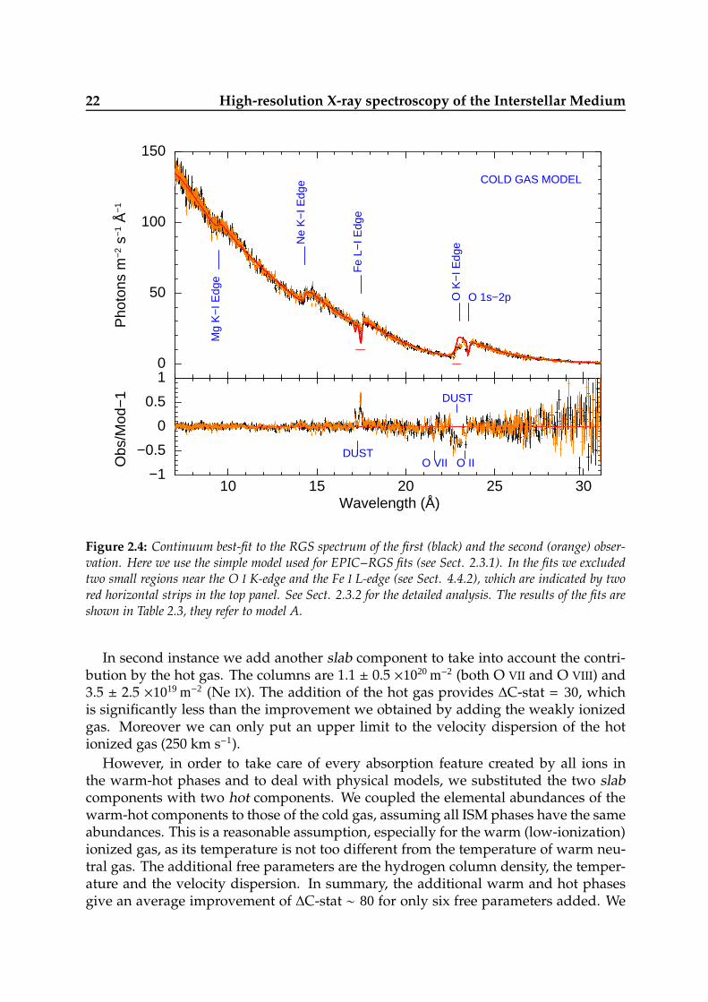
Table 2.3: RGS spectral fits to the persistent emission. (a) We give the separate fits for the two observa-tions only for Model A in order to show that they are consistent within the errors and thus can be fittedtogether. C-Stat / dof (*) refers to the statistics obtained by including the wavelength ranges 17.2-17.7Å and 22.7-23.2 Å, which in fits are ignored except in the case of the complete model. (b) All columns forthe dabs and amol components are reported in units of 1021m−2. (c) Each amol component is displayedtogether with its molecular index as reported in Table A.1.
Mod A (a) Mod B Mod C
Component Parameter OBS 1 OBS 2 OBS 1+2 OBS 1+2 OBS 1+2
Cold
NH (1025m−2) 4.18± 0.01 4.22± 0.07 4.21± 0.09 3.88± 0.07 3.94± 0.05
kT (10−4 keV) 5.90± 0.14 6.13± 0.12 6.02± 0.09 6.04± 0.10 8.6± 0.4
σV (km s−1) 27± 15 18± 6 13± 7 < 12.6 < 24
O 1.30± 0.02 1.29± 0.02 1.29± 0.01 1.29± 0.02 1.17± 0.03
Ne 2.08± 0.04 1.86± 0.07 1.95± 0.07 2.19± 0.10 1.75± 0.11
Mg 2.27± 0.12 2.14± 0.16 2.21± 0.16 1.93± 0.15 1.30± 0.25
Fe 1.39± 0.02 1.42± 0.06 1.39± 0.05 1.65± 0.08 < 0.1
Warm
NH (1025m−2) - - - 0.46± 0.06 0.15± 0.05
kT (10−3 keV) - - - 5.4± 0.3 4.5± 0.5
σV (km s−1) - - - 50± 25 < 150
Hot
NH (1025m−2) - - - 0.042± 0.008 0.047± 0.011
kT (keV) - - - 0.20± 0.02 0.20± 0.03
σV (km s−1) - - - < 160 < 200
Dabs (b) NFe - - - - 2.6± 0.1
NMg - - - - 2.3± 0.1
Amol (b, c)
NO (i=14, Silicates) - - - - 2.5± 0.5
NO (i=7, H2O Ice) - - - - < 0.7
NO (i=2, CO) - - - - < 0.4
NO (i=23, Aluminates) - - - - < 0.4
StatisticsC-Stat / dof 2239/1595 2170/1589 4587/3232 4435/3226 4818/3398
C-Stat / dof (*) 2930/1684 3040/1710 5757/3410 6064/3404 4818/3398
label such a three-gas model as Model B and display all results in Table 2.3. We plotthe individual absorption edges of O, Fe, Ne and Mg in Figs. 2.5, 2.6, 2.7 and 2.8, re-spectively. We discuss these results in Sect. 5.5.2. The predicted deviations near theoxygen and iron edges, clearly seen in Fig. 2.5 and 2.6, still confirm that pure inter-stellar gas cannot reproduce all the absorption features and that we need to take intoaccount different states of matter, such as solids.
Finally, we also considered the model where the cold gas component is forced to beneutral by freezing its temperature to 5× 10⁻⁴ keV, i.e. 5 800K. In this case, we got analmost equal fit (C-stat/dof = 4466/3227), with the exception that the warm componenthas a significantly lower temperature (∼ 1.4 × 10⁻³ keV, i.e. 10− 20 000K), to accountfor the O II that in our nominal fit is partially produced by the cold component. Thistemperature value is more representative than our previous value of 5.4× 10⁻³ keV forthe warm ionized gas in the ISM (Ferriere 2001). However, both fits are acceptable,thus we report only results obtained with the cold-gas temperature as free parameterin Table 2.3.
24 High-resolution X-ray spectroscopy of the Interstellar Medium
21 22 23 24
05
1015
20
Flu
x (
Pho
tons
m−
2 s−
1 Å
−1 )
Wavelength (Å)
O I
O II
O K−I EdgeO I + O III
O VII
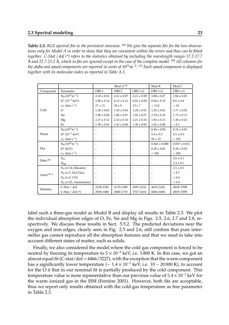
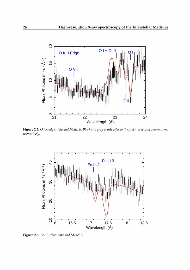
Figure 2.5: O I K-edge: data and Model B. Black and grey points refer to the first and second observation,respectively.
16 16.5 17 17.5 18 18.51020
3040
Flu
x (
Pho
tons
m−
2 s−
1 Å
−1 )
Wavelength (Å)
Fe I L3Fe I L2
Figure 2.6: Fe I L-edge: data and Model B.
2.3 Spectral modeling 25
13.5 14 14.5 15
4050
60
Flu
x (
Pho
tons
m−
2 s−
1 Å
−1 )
Wavelength (Å)
Ne IX
Ne K−I
Ne IIINe II
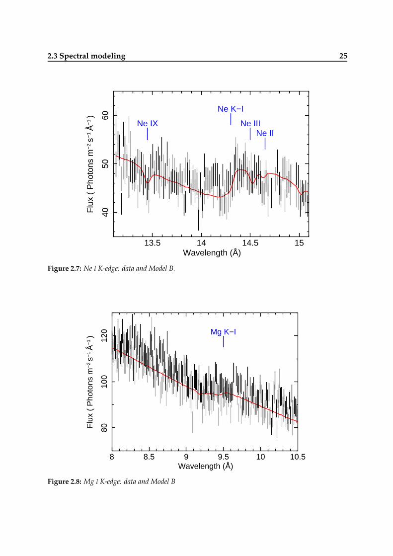
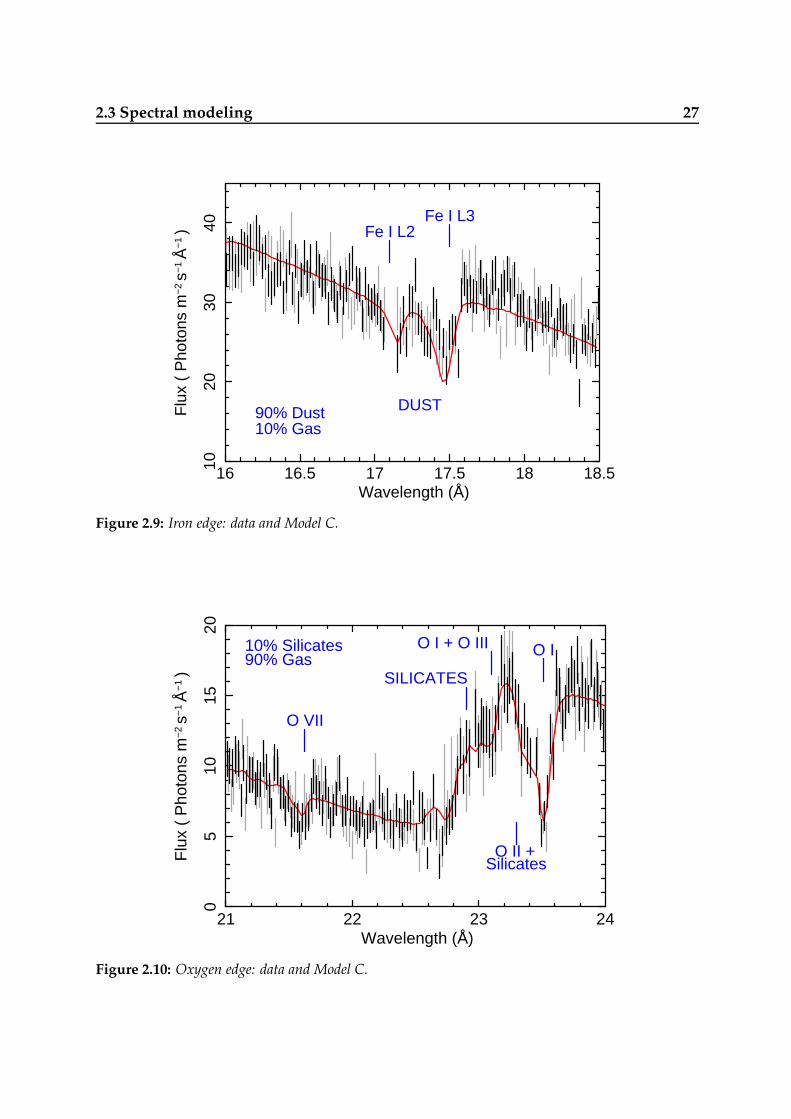
Figure 2.7: Ne I K-edge: data and Model B.
8 8.5 9 9.5 10 10.5
8010
012
0
Flu
x (
Pho
tons
m−
2 s−
1 Å
−1 )
Wavelength (Å)
Mg K−I
Figure 2.8: Mg I K-edge: data and Model B
26 High-resolution X-ray spectroscopy of the Interstellar Medium
Fine structures: Dust and molecules
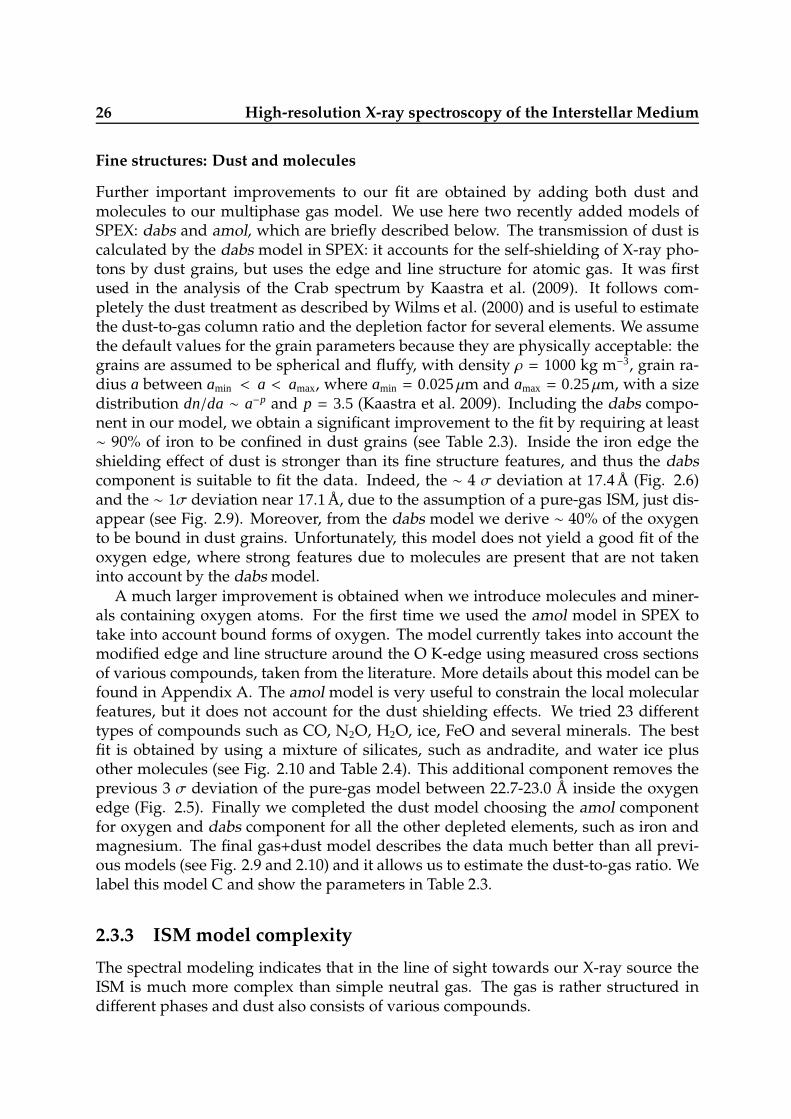
Further important improvements to our fit are obtained by adding both dust andmolecules to our multiphase gas model. We use here two recently added models ofSPEX: dabs and amol, which are briefly described below. The transmission of dust iscalculated by the dabs model in SPEX: it accounts for the self-shielding of X-ray pho-tons by dust grains, but uses the edge and line structure for atomic gas. It was firstused in the analysis of the Crab spectrum by Kaastra et al. (2009). It follows com-pletely the dust treatment as described by Wilms et al. (2000) and is useful to estimatethe dust-to-gas column ratio and the depletion factor for several elements. We assumethe default values for the grain parameters because they are physically acceptable: thegrains are assumed to be spherical and fluffy, with density ρ = 1000kg m−3, grain ra-dius a between amin < a < amax, where amin = 0.025µm and amax = 0.25µm, with a sizedistribution dn/da ∼ a−p and p = 3.5 (Kaastra et al. 2009). Including the dabs compo-nent in our model, we obtain a significant improvement to the fit by requiring at least∼ 90% of iron to be confined in dust grains (see Table 2.3). Inside the iron edge theshielding effect of dust is stronger than its fine structure features, and thus the dabscomponent is suitable to fit the data. Indeed, the ∼ 4 σ deviation at 17.4 Å (Fig. 2.6)and the ∼ 1σ deviation near 17.1 Å, due to the assumption of a pure-gas ISM, just dis-appear (see Fig. 2.9). Moreover, from the dabs model we derive ∼ 40% of the oxygento be bound in dust grains. Unfortunately, this model does not yield a good fit of theoxygen edge, where strong features due to molecules are present that are not takeninto account by the dabs model.
A much larger improvement is obtained when we introduce molecules and miner-als containing oxygen atoms. For the first time we used the amol model in SPEX totake into account bound forms of oxygen. The model currently takes into account themodified edge and line structure around the O K-edge using measured cross sectionsof various compounds, taken from the literature. More details about this model can befound in Appendix A. The amol model is very useful to constrain the local molecularfeatures, but it does not account for the dust shielding effects. We tried 23 differenttypes of compounds such as CO, N2O, H2O, ice, FeO and several minerals. The bestfit is obtained by using a mixture of silicates, such as andradite, and water ice plusother molecules (see Fig. 2.10 and Table 2.4). This additional component removes theprevious 3 σ deviation of the pure-gas model between 22.7-23.0 Å inside the oxygenedge (Fig. 2.5). Finally we completed the dust model choosing the amol componentfor oxygen and dabs component for all the other depleted elements, such as iron andmagnesium. The final gas+dust model describes the data much better than all previ-ous models (see Fig. 2.9 and 2.10) and it allows us to estimate the dust-to-gas ratio. Welabel this model C and show the parameters in Table 2.3.
2.3.3 ISM model complexity
The spectral modeling indicates that in the line of sight towards our X-ray source theISM is much more complex than simple neutral gas. The gas is rather structured indifferent phases and dust also consists of various compounds.
2.3 Spectral modeling 27
16 16.5 17 17.5 18 18.51020
3040
Flu
x (
Pho
tons
m−
2 s−
1 Å
−1 )
Wavelength (Å)
Fe I L3Fe I L2
DUST90% Dust10% Gas
Figure 2.9: Iron edge: data and Model C.
21 22 23 24
05
1015
20
Flu
x (
Pho
tons
m−
2 s−
1 Å
−1 )
Wavelength (Å)
O I
O II +
10% Silicates O I + O III
O VII
SILICATES
Silicates
90% Gas
Figure 2.10: Oxygen edge: data and Model C.

28 High-resolution X-ray spectroscopy of the Interstellar Medium
The gas consists of three components (see Table 2.3): cold gas with a temperaturekT ∼ 5−10×10−4 keV (5.8−10 ×103 K), warm ionized gas with kT ∼ 1−5×10⁻³ keV (1−6×10⁴ K) and hot ionized gas with kT ∼ 0.2keV (& 2× 10⁶ K). The column densities NH
of these three components span over 2 orders of magnitude: the cold gas accounts for∼ 90−95% of the total column N tot
H , NwarmH ∼ 5−10% of N tot
H , while the hot gas contributes∼ 1%.
The warm component produces the low-ionization absorption lines of O II and O III,at 23.35 Å and 23.1 Å respectively (see Fig. 2.5). It also provides a better modeling ofthe neon edge (see Fig. 2.7). Using model B we estimate NO II = 2.0 ± 0.5 × 10²¹ m−2
and NO III = 1.4 ± 0.5 × 10²¹ m−2, respectively ∼ 7% and ∼ 5% of the total oxygen col-umn. However, the derived column density of the warm ionized gas is affected by thepresence of dust and molecules in the line of sight. Indeed, the absorption featuresthat we see near 23.35 Å and 23.1 Å are contaminated by dust and molecule effects.Contributions from dust and molecules (Model C in Table 2.3) are confirmed by theimprovements to the fit (see also Fig. 2.9 and 2.10), and the column density of thewarm gas is finally reduced to about 5% of the full gas column (see Table 2.4).
The column density of hot gas is about two orders of magnitude lower than the coldgas column and its temperature is around two million K. As expected, the hotter gashas a higher velocity dispersion (see Table 2.3). The hot gas model gives a good fit ofthe O VII absorption line at 21.6 Å, together with the small feature at 13.4 Å producedby Ne IX.
According to the analysis of the oxygen edge, the solid phase of the ISM towardsGS 1826−238 consists of a mixture of minerals (such as andradite silicates) and tracesof CO and water ice. We cannot yet distinguish between amorphous and crystallinephases. As reported in Table 2.4 the bulk of the oxygen, ∼ 90%, appears to be in thegas phase, while the remaining ∼ 10% is made mostly of solids, such as silicates andwater ice. Obviously, there could be substances able to reproduce these features in thespectrum other than our few dozen test molecules. For the iron, instead, we obtain adifferent composition: at least ∼ 90%of Fe appears to be bound in dust grains. In ourdust model we assume a depletion factor of 0.8 for magnesium, as suggested by Wilmset al. (2000). The derived gas (2.0± 0.4× 10²¹ m−2) and dust (2.3± 0.1× 10²¹ m−2) columndensities for the Mg are identical within the errors (see also Table 2.3).
2.3.4 ISM abundances
We estimated the abundances of Mg, Ne, Fe, O, and N (Table 2.5). The column densityof each element refers to the sum of the contributions from all gas and dust phases.The abundances do not differ significantly between the two observations (see Table2.3). This is expected if the absorption is mainly caused by the interstellar medium,because the ISM is stable on short timescales. The zero shift of the O I line, the positionof the O, Fe, Ne, and Mg edges (see Fig. 2.5 to 2.10) and the low velocity dispersionsuggest that the absorber matter is a mixture of gas and dust without outflows or in-flows, not broadened owing to Keplerian motion around the X-ray source. This is alsoconsistent with an ISM origin. For a more detailed discussion on the abundances andcomparisons with previous work see Sect. 2.4.3.
2.3 Spectral modeling 29
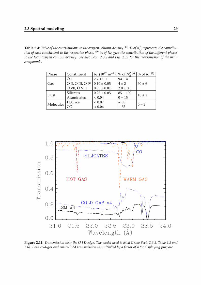
Table 2.4: Table of the contributions to the oxygen column-density. (a) % of N pO represents the contribu-
tion of each constituent to the respective phase. (b) % of NO give the contribution of the different phasesto the total oxygen column density. See also Sect. 2.3.2 and Fig. 2.11 for the transmission of the maincompounds.
Phase Constituent NO (1022 m−2) % of N pO
(a) % of NO(b)
GasO I 2.7± 0.1 94± 4O II, O III, O IV 0.10± 0.05 4± 2 90± 6O VII, O VIII 0.05± 0.01 2.0± 0.5
DustSilicates 0.25± 0.05 85− 100
10± 2Aluminates < 0.04 0− 15
MoleculesH2O ice < 0.07 ∼ 65
0− 2CO < 0.04 ∼ 35
Figure 2.11: Transmission near the O I K-edge. The model used is Mod C (see Sect. 2.3.2, Table 2.3 and2.6). Both cold-gas and entire-ISM transmission is multiplied by a factor of 4 for displaying purpose.
30 High-resolution X-ray spectroscopy of the Interstellar Medium
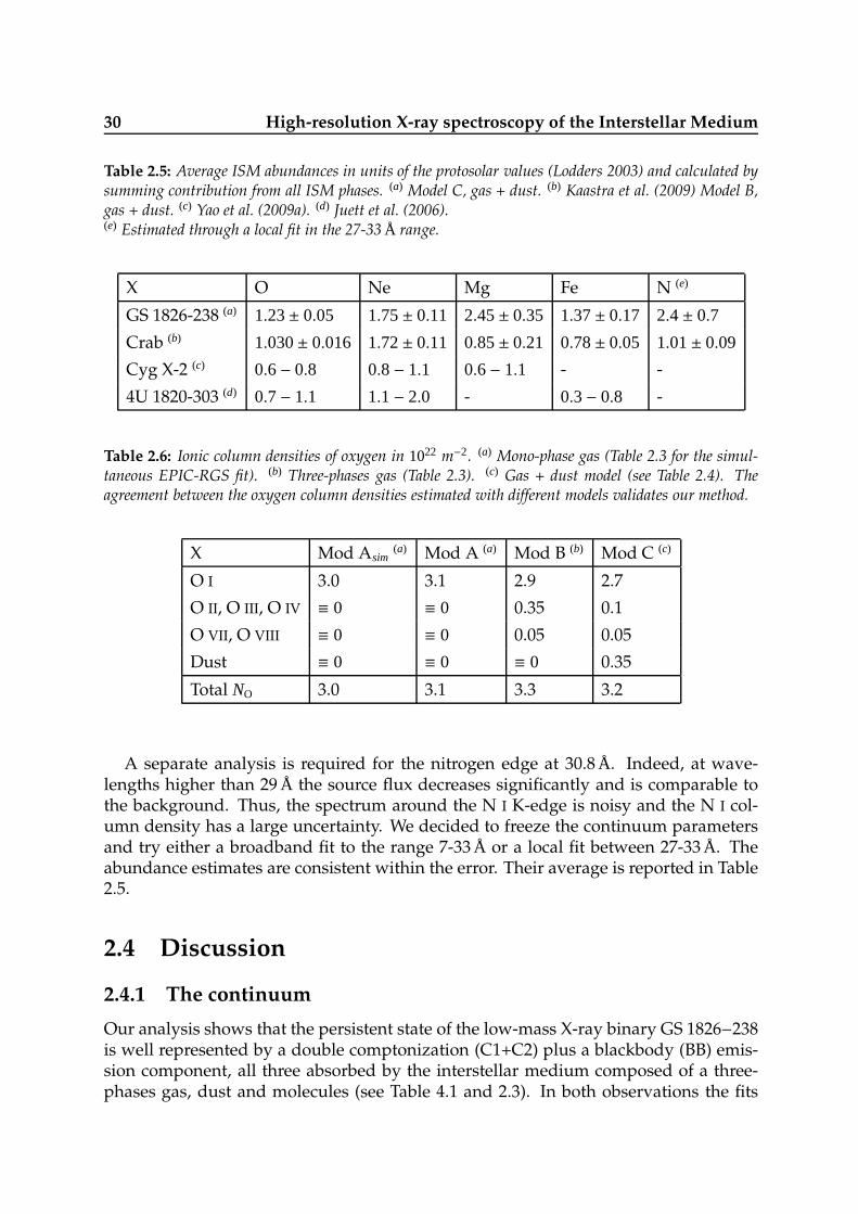
Table 2.5: Average ISM abundances in units of the protosolar values (Lodders 2003) and calculated bysumming contribution from all ISM phases. (a) Model C, gas + dust. (b) Kaastra et al. (2009) Model B,gas + dust. (c) Yao et al. (2009a). (d) Juett et al. (2006).(e) Estimated through a local fit in the 27-33 Å range.
X O Ne Mg Fe N (e)
GS 1826-238 (a) 1.23± 0.05 1.75± 0.11 2.45± 0.35 1.37± 0.17 2.4± 0.7
Crab (b) 1.030± 0.016 1.72± 0.11 0.85± 0.21 0.78± 0.05 1.01± 0.09
Cyg X-2 (c) 0.6− 0.8 0.8− 1.1 0.6− 1.1 - -
4U 1820-303 (d) 0.7− 1.1 1.1− 2.0 - 0.3− 0.8 -
Table 2.6: Ionic column densities of oxygen in 1022 m−2. (a) Mono-phase gas (Table 2.3 for the simul-taneous EPIC-RGS fit). (b) Three-phases gas (Table 2.3). (c) Gas + dust model (see Table 2.4). Theagreement between the oxygen column densities estimated with different models validates our method.
X Mod Asim(a) Mod A (a) Mod B (b) Mod C (c)
O I 3.0 3.1 2.9 2.7
O II, O III, O IV ≡ 0 ≡ 0 0.35 0.1
O VII, O VIII ≡ 0 ≡ 0 0.05 0.05
Dust ≡ 0 ≡ 0 ≡ 0 0.35
Total NO 3.0 3.1 3.3 3.2
A separate analysis is required for the nitrogen edge at 30.8 Å. Indeed, at wave-lengths higher than 29 Å the source flux decreases significantly and is comparable tothe background. Thus, the spectrum around the N I K-edge is noisy and the N I col-umn density has a large uncertainty. We decided to freeze the continuum parametersand try either a broadband fit to the range 7-33 Å or a local fit between 27-33 Å. Theabundance estimates are consistent within the error. Their average is reported in Table2.5.
2.4 Discussion
2.4.1 The continuum
Our analysis shows that the persistent state of the low-mass X-ray binary GS 1826−238is well represented by a double comptonization (C1+C2) plus a blackbody (BB) emis-sion component, all three absorbed by the interstellar medium composed of a three-phases gas, dust and molecules (see Table 4.1 and 2.3). In both observations the fits
2.4 Discussion 31
agree: all the ISM parameters appear to be fully consistent, thus we can discuss theresults from the simultaneous fit of the high-resolution RGS data.
2.4.2 ISM structure
In Sect. 5.5.2 we showed that in our line of sight the ISM has a clear multiphase struc-ture. There are media with different ionization states, dust grains, and molecules.As confirmed by Fig. 2.11, the bulk of the matter responsible for X-ray absorption isfound in the form of cold gas with a temperature ∼ 7 000 K and low-velocity dispersion(σV . 13 km s−1). At this temperature the gas is almost neutral: only iron and magne-sium are partially ionized. Part of the cold matter is found in solid compounds, such asdust grains and molecules. Most of the iron is bound in dust grains. About 10% of theoxygen is found in compounds: the silicates contribute up to ∼ 80% of this phase, whilethe remaining fraction consists of a mixture of other oxides (such as iron aluminates)together with ices and CO molecules in similar quantities (see Table 2.4). The best fit isobtained using as compound the andradite silicate Ca3 Fe2 (SiO4)3, but we need highersignal-to-noise data to distinguish among the different silicates, because also olivineand pyroxene are good candidates. Moreover, at the present stage our model doesnot take into account simultaneously the shielding and fine structure effects of oxygencompounds, thus the fraction of oxygen bound in solids could be higher, e.g. up to 40%(see Sect. 2.3.2). However, we are working to the development of models that take intoaccount all the possible effects and we postpone a deeper analysis of the oxygen dustphase to a forthcoming paper.
About 5% of the gas is ionized (see Mod C in Table 2.3). Most of it is a warm plasmawith T ∼ 10− 50 000K. It has a low-ionization degree and accounts for the interstellarO II and O III. Only 1-2% of the ISM gas appears to be highly ionized. Such a hot plasmareaches temperatures of ∼ 2×10⁶ K and contributes to all O VII and O VIII present in theISM. As we expect, the higher the temperature of the gas phase, the higher its velocitydispersion. Unfortunately the velocity dispersion is not well constrained, especiallyfor the hot ionized gas. This is not surprising because the lines are unresolved.
2.4.3 Comparison with previous results
ISM constituents
The average total column density of the multi-phase gas we estimate is about (4.14±0.07)×1025 m−2. This is not consistent with the value of (3.19±0.01)×1025 m−2 found byThompson et al. (2008). They combined data from Chandra, XMM-Newton and RXTEin the 0.5−100keV band, but we know that the bulk of the absorption is at lower energy.Instead we have used both EPIC and RGS data. The latter detector has a higher spectralresolution between 0.3− 2keV and allows us to better estimate the absorption column.Also, Thompson et al. (2008) used the Morrison & McCammon (1983) model to fit theabsorbing medium, which takes into account only contribution by cold neutral gas. InSect. 2.3.1 we have shown that this model is not optimal, because it does not includelines. Furthermore, abundances and temperature cannot be free parameters. Instead
32 High-resolution X-ray spectroscopy of the Interstellar Medium
our estimate of NH is obtained by summing the contribution from all phases of the gasand by accounting for all absorption features found in the spectrum.
The multiphase structure of the ISM that we constrained is consistent with recentresults (Ferriere 2001; Yao & Wang 2006; Yao et al. 2009a). First of all, there is a goodagreement in the fractions between the cold, warm, and hot phases of the gas. Inparticular the estimated amount of O VII, ∼ 1.6 × 10²⁰ m−2, is fully consistent with thevalue found by Yao & Wang (2006) by fitting both O VII 1s−2p and 1s−3p lines in thespectrum of 4U 1820−303, which is another LMXB near the center of the Galaxy. Thehot gas accounts for 1 − 2% of the total column density and represents the averagefraction of hot plasma in the Galaxy. Indeed it agrees with previous estimates and canbe fully explained by the heating of supernovae (McCammon & Sanders 1990b). Thevelocity dispersion σV estimates agree with recent work. Yao & Wang (2006) combinedoxygen and neon ionization lines in the Chandra spectrum of the LMXB 4U 1820−303,obtaining σV < 350km s−1. Juett et al. (2004) found σV < 200km s−1 from oxygen linesfits to the Chandra spectra of several LMXBs.
Moreover, we found clear indications of dust depletion in some heavy elements,such as oxygen, iron, and magnesium. According to the different dust models that weused (dabs and dabs+amol), we find ∼ 50% of Mg, more than 90% of Fe and 10−40% ofoxygen in the form of dust grains and molecular compounds. These results are mostlyconsistent with previous estimates (Wilms et al. 2000; Kaastra et al. 2009). The irondust-to-gas ratio found towards GS 1826−238 is among the highest measured in theGalaxy. Williams & Taylor (1996) showed that the higher the density of a molecularcloud, the higher is the probability of forming dust and molecules from gas particles.Thus the higher dust-to-gas ratio we estimated towards the center of the Galaxy sug-gests high-density regions.
The presence of silicates and ice in the ISM, constrained by the O I K-edge analysis, issupported by other work. Paerels et al. (2001) found similar features within 22.7−23.0 Åin the spectrum of the LMXB X0614+091, and they argued that it should be due to ironoxides or oxygen generally bound in dust. Costantini et al. (2005) found indicationsof silicates such as olivine and pyroxene by modeling the feature of the scattering haloof Cyg X−2. Recently, de Vries & Costantini (2009) found evidence for EXAFS in theshort-wavelength side of the oxygen edge in the spectrum of Sco X−1, and their resultssuggest the presence of amorphous water ice.
We have checked CO surveys (Dame et al. 2001) in order to test the presence ofmolecular clouds. There is no clear evidence for these clouds in our line of sight(x, y)GAL ∼ (9.3,−6.1), while there is an important amount of diffuse dust (see alsoSchlegel et al. 1998). This is consistent with the fact that we can only put upper limitsto ice and CO columns. Thus the absorption should arise from a solid phase consistingmostly of minerals.
ISM abundances
The abundances are displayed in Table 2.5, they are reported relative to the recom-mended protosolar values of Lodders (2003). We also show the abundances obtainedby Juett et al. (2006) towards the LMXB 4U 1820−303, which like GS 1826−238 is close

2.4 Discussion 33
Figure 2.12: Map of the X-ray sources compared in this paper. GC is the Galactic Center and the Sunis assumed to be 8.5 kpc far away from it.
to the Galactic center. Even more interesting is the comparison with the abundancesestimated by Kaastra et al. (2009) in the direction of the Crab nebula and those esti-mated by Yao et al. (2009a) towards Cyg X−2, which are two different lines of sight inour Galaxy (see the map in Fig. 5.1).
The derived abundances slightly depend on the model used: the pure-gas modeland the complete gas+dust model yield different results on Ne, Fe, and Mg (Table 2.3).First, their abundances are more uncertain than the oxygen abundance. Secondly, Feand Mg are the most depleted elements: as dust grains give rise to absorption featuresdifferent from gas particles, modeling the edges of highly depleted elements providesdifferent results if we account for dust effects or not. These deviations are probablyintensified because we observed through a high-density region: here high metal de-pletion is expected (Williams & Taylor 1996).
All the heavy elements are over-abundant with respect to the protosolar values.Neon is over-abundant by a factor ∼ 1.7, as found by Kaastra et al. (2009) in the XMM-Newton observations of the Crab nebula. The solar abundance of neon is probablyunder-estimated (see Lodders & Palme 2009), so our estimate may be not really differ-ent from the real solar value. As we will show in the next paragraph, the metallicitygradient could also be responsible for part of the Ne over-abundance.
The reason for the over-abundances of O, Fe, and Mg is rather different from theneon excess. First of all, we are able to measure both gas and dust contributions for O,Fe and Mg, without the risk of missing important fractions. Secondly, deviations in theabundances with respect to the average Galactic values are also due to their metallicity
34 High-resolution X-ray spectroscopy of the Interstellar Medium
gradient. If A(X) is the abundance of a certain element X in the vicinity of GS 1826−238,we can write (see Esteban et al. 2005)
A(X)A(X)⊙
= 10αX (DGS−D⊙), (2.1)
where D⊙ and DGS are the galactocentric radii of the Sun and GS 1826−238, respec-tively ∼ 8.5 kpc and ∼ 2 kpc; αX is the abundance gradient of the element along theline of sight and A(X)⊙ is its abundance near the Sun. In this way, we can compare ourestimates of abundance changes with the values predicted by the gradient estimates.Unfortunately, the gradient estimates in the literature are quite uncertain and are avail-able only for a limited range of radii, i.e. between 4-16 kpc (see Pedicelli et al. 2009).Thus we can trust only in the abundance changes in 4 − 5kpc along our line of sight.Moreover, the column density estimated for each element refers to its integral alongthe line of sight, where we also expect a density increase towards the Galactic Center.Because the density increases towards the Galactic center, the predicted abundance atthe galactocentric distance of GS 1826−238 should be close to the weighted averageabundance along the sightline:
• Oxygen is over-abundant by about 20−30% (see Table 2.5). According to Estebanet al. (2005), the oxygen gradient is αO = (−0.04±0.01) kpc−1, which should providean increment (equation 2.1) of at least ∼ 32% in the oxygen abundance. This isconsistent with our estimate.
• The iron abundance ∼ 1.20−1.54 (see Table 2.5) almost agrees with the & 50%increment derived by the accepted iron gradient in the Galactic disk αFe = (−0.06±0.02) kpc−1 (Friel et al. 2002; Pedicelli et al. 2009).
• Neon is over-abundant by more than 70%. It is difficult to compare it withthe Galactic gradient because this is quite uncertain, on average αNe = (−0.06±0.04) kpc−1 (Simpson et al. 1995; Maciel & Quireza 1999). From equation (2.1) wepredict a lower limit A(Ne) ∼ 1.3. The sum of this a value to the revisited pro-tosolar abundance (∆A(Ne) ∼ 30 %, see Lodders & Palme 2009) provides A(Ne)∼ 1.6, which is fully consistent with our estimate. This result suggests that theneon over-abundance that we constrain is due to both the Galactic gradient andthe previous under-estimate found in the literature.
• Nitrogen shows a steeper Galactic gradient of about ∼ −0.08 kpc−1 (Gummersbachet al. 1998), which provides ∆A(N) ∼ 100 % (equation 2.1) and agrees with ourestimate (see Table 2.5). Of course, both of them are quite uncertain and we arenot able to provide more information.
• Also magnesium should be at least twice the protosolar value as we found (seeTable 2.5). However, it is difficult to compare our result with the Mg Galacticgradient found in the literature, because the results differ widely in the literature(Rolleston et al. 2000). According to Gummersbach et al. (1998) αMg ∼ −0.08 kpc−1,which together with equation (2.1) implies an abundance increment of at least100%. This is fully consistent with what we found.
2.5 Conclusion 35
The iron and oxygen abundances towards 4U 1820−303 (Table 2.5) appear to dis-agree with our results despite its similar location near the Galactic center. Juett et al.(2006) attribute this low iron abundance to depletion into dust grains in the interstellarmedium, and they also report that oxygen could be middle-depleted. In Sect. 2.3.2we have shown that iron is among the most depleted elements in the ISM, oxygen isalso partially depleted and a pure-gas model cannot reproduce all the ISM spectral fea-tures. This indicates that the differences between the Fe and O abundances are due tothe capability of our gas+dust model to measure the contribution from solid phases,which are absent in the pure-gas model of Juett et al. (2004, 2006).
The Crab nebula is relatively close to the Solar System, i.e. ∼ 2 kpc, but opposite tothe Galactic Center (see Fig. 5.1). Thus we expect abundances close to the protosolarvalues of Lodders (2003), which is just what Kaastra et al. (2009) found.
The source LMXB Cyg X-2 is also far away from the center of the Galaxy and about10 kpc away from the Sun. The abundances estimated for this source are lower thanthose measured towards the Crab and GS 1826−238 (see Table 2.5). This agrees withthe assumed abundance gradients we have discussed.
In summary, the differences with respect the protosolar abundances that we estimateare consistent with the literature. The increase of metallicity towards the center of theGalaxy should be due to evolutionary effects like supernovae explosions, which enrichthe ISM with heavy elements, especially in the higher density region of the bulge andthe disk of our Galaxy. A deeper analysis is required: we need to study more sources,even in the same region, and further improve our models in order to account for everycontribution to the column densities.
2.5 Conclusion
We have presented a complete treatment of the interstellar medium towards the low-mass X-ray binary GS 1826−238, which is a bright X-ray source near the Galactic Center.We have shown that in the line of sight the ISM is composed of a complex mixture of amulti-phase gas, dust, and molecules.
The gas is almost neutral and the ionization degree is about 5%. Significant fractionsof the column density of some heavy elements are in the form of molecules or dustgrains: at least 10% of oxygen, 50% of magnesium, and 90% of iron. Such a solid phaseshould consist of a mixture of silicates (& 60%), CO (. 10%), ice (. 20%) and other ironoxides (. 10%).
We have found over-abundances for all the elements for which we have been ableto measure the individual column density. The Ne over-abundance that we estimateis consistent with other recent work in different lines of sight, such as towards theCrab (Kaastra et al. 2009), suggesting that the solar value is underestimated. However,our agreement with the predicted Ne gradient in the Galaxy is also consistent with anabundance increase owing to stellar evolution: towards the Galactic center there arehigh-density regions with evolved star that could have enriched the ISM with heavyelements such as neon.
36 High-resolution X-ray spectroscopy of the Interstellar Medium
Differently from the previous X-ray spectroscopy work, we have found over-abun-dances for oxygen (1.2), iron (1.4) and magnesium (2.4). These elements are also inthe form of dust and molecules. Thus our estimates are partially due to the fact thatwe are also able to measure the contributions from the solid phase. The abundance ofmetals agrees with the metallicity gradients and shows the chemical inhomogeneity ofthe interstellar medium.
The diagnostic of the ISM constituents fits the predicted models for both its ther-mal and chemical structures, showing a good agreement with the current state of art(Ferriere 2001). The dust column is consistent with the multi-wavelength, X-ray versusIR, observations. All this supports our research method and justifies new observationsand analyses of other sources in different lines of sight. These analyses provide indeeda better mapping of the ISM and a deeper study of its chemical composition, togetherwith its role in the evolution of the entire Galaxy.
Acknowledgements
We are grateful to Jean in’t Zand for the useful discussion and clarification about thephysics of low-mass X-ray binaries. This work is based on observations obtained withXMM-Newton, an ESA science mission with instruments and contributions directlyfunded by ESA Member States and the USA (NASA). SRON is supported financiallyby NWO, the Netherlands Organization for Scientific Research.
Chapter 3
A phenomenological model for theX-ray spectrum of nova V2491 Cygni
C. Pinto1, J.-U. Ness2, F. Verbunt3, J. S. Kaastra1, E. Costantini1, R. G. Detmers1
1 SRON Netherlands Institute for Space Research, Utrecht, The Netherlands2 ESAC European Space Astronomy Center, Villanueva de la Canada, Madrid, Spain3 Department of Astrophysics, Radboud University, Nijmegen, The Netherlands
Received 9 August 2011 / Accepted 10 June 2012
Published in Astronomy & Astrophysics, volume 543, pages A134–144, 2012
Abstract
The X-ray flux of nova V2491 Cyg reached a maximum some forty days after opticalmaximum. The X-ray spectrum at that time, obtained with the RGS of XMM-Newton,shows deep, blue-shifted absorption by ions of a wide range of ionization. We showthat the deep absorption lines of the X-ray spectrum at maximum, and those observednine days later, are well described by a phenomenological model with emission from acentral blackbody and from a collisionally ionized plasma (CIE). The blackbody spec-trum (BB) is absorbed by three main highly ionized expanding shells; the CIE andBB are absorbed by cold circumstellar and interstellar matter that includes dust. Theoutflow density does not decrease monotonically with distance. The abundances ofthe shells indicate that they were ejected from an O-Ne white dwarf. We show that
38 A phenomenological model for the X-ray spectrum of nova V2491 Cygni
the variations on time scales of hours in the X-ray spectrum are caused by a combina-tion of variation in the central source and in the column density of the ionized shells.Our phenomenological model gives the best description so far of the supersoft X-rayspectrum of nova V2491 Cyg, but underpredicts, by a large factor, the optical and ul-traviolet flux. The X-ray part of the spectrum must originate from a very different layerin the expanding envelope, presumably much closer to the white dwarf than the layersresponsible for the optical/ultraviolet spectrum. This is confirmed by the absence ofany correlation between the X-ray and UV/optical observed fluxes.
3.1 Introduction
The sensitivity to soft X-rays of the EXOSAT satellite enabled the first discovery of X-rays from a classical nova, GQ Mus, in April 1984 (Oegelman et al. 1984). The ROSATsatellite detected it almost eight years later, in February 1992, and found it to have avery soft blackbody-like spectrum with kTeff ∼ 28eV (Oegelman et al. 1993). ROSATobservations of other novae in our galaxy showed that only a small fraction of novaeare detected in X-rays (Oegelman et al. 1993; Orio et al. 2001).
The spectrum of GQ Mus is very soft, comparable to the spectra of a new class ofsupersoft X-ray sources (SSS) discovered with ROSAT in the Large Magellanic Cloud,with temperatures ∼< 100 eV in blackbody fits to their spectra (Trumper et al. 1991;Greiner et al. 1991). The favored explanation for the X-ray spectra of the supersoftsources such as for GQ Mus is hydrogen burning at the surface of a white dwarf, ofmaterial accreted from a companion star. The class of supersoft X-ray sources showsa large variety, some sources being permanent and others transient, and with widedifferent types of companion stars (see review by Kahabka & van den Heuvel 1997).Observation campaigns with ROSAT, XMM-Newton and Chandra in M31 show thatmost of the supersoft sources are classical novae (Pietsch et al. 2005; Henze et al. 2010).Recently, Henze et al. (2011) argued that the high fraction of novae without detectedSSS emission might be explained by the incomplete coverage.
The model fits of the supersoft X-ray spectra have become increasingly sophisticatedover the years. Blackbody fits indicated high super-Eddington luminosities for theROSAT sources. Heise et al. (1994) showed that the fit of local thermodynamic equilib-rium (LTE) model atmospheres to the ROSAT data brought their bolometric luminositybelow the Eddington limit for temperatures ≤ 60eV. For temperatures ≥ 100eV, Hart-mann & Heise (1997) showed that the differences between bolometric luminosities forROSAT supersoft sources derived from blackbody, LTE and NLTE models are muchsmaller, the main difference being that NLTE models may give appreciable flux above0.4 keV (i.e. in the ‘hard’ ROSAT band). A new level of sophistication is reached byPetz et al. (2005), who fit NLTE model spectra of expanding atmospheres, thus takinginto account the outflow inherent in the nova phenomenon. Even the most sophisti-cated model fails to fit the observed continuum of the nova V4743 Sgr at λ < 30 Å, andalso does not match the depth of the absorption lines (Fig. 3 of Petz et al. 2005; Rauch& Werner 2010). With regard to the X-ray spectra of V2491 Cyg, the best publishedatmosphere model does not reproduce the observed line velocities or the observed line
3.1 Introduction 39
depths, as clearly visible in Fig. 11 of Ness et al. (2011), for example in the N VII 1s-2p line at 24.8 Å. Atmosphere models so far also fail to reproduce the wide range ofionization levels simultaneously present in the observed spectra: e.g. O V to O VIII inV2491 Cyg (see Figs. 3.1-3.4 below).
What is the reason for this failure? If there are shocks in the expanding nova enve-lope, the assumption of a standard atmosphere whose density decreases monotonicallyoutward, breaks down. The rapid X-ray variability observed in some novae indicatesthat the expanding envelope and/or the luminosity from the deeper layers are not sta-tionary and/or not spherically symmetric, invalidating another assumption in atmo-sphere models. In this paper we therefore investigate a pilot model of a quite differentnature, in which separate expanding shells absorb the spectrum of an underlying cen-tral source. In this first study, we describe the central source as a blackbody spectrum.We apply our simple model to the XMM-Newton RGS spectra obtained from the novaV2491 Cyg to investigate whether this model gives a better description of the contin-uum and line absorption; whether the short-term variability is due to changes in thesource or in the absorption; and whether the model allows determining of the chemicalabundances in the expanding envelope.
Nova V2491 Cyg was discovered on April 10, 2008, at V = 7.7 (Nakano et al. 2008).The optical flux declined from this peak in the course of the following months, inter-rupted by a brief second maximum at the end of April. Ultraviolet and X-ray fluxesof the V2491 Cyg were obtained with the Swift satellite: the ultraviolet flux declinedin tandem with the optical flux (measured through May and June), whereas the X-rayluminosity rose from a marginal detection on April 11 to a peak more than a thousandtimes brighter some 40 days later (Page et al. 2010). Lightcurves of optical, ultravioletand X-ray are shown in Fig. 4 of Page et al. (2010). In the Swift X-ray range (0.3-8 keV)the spectrum peaks strongly near 0.4-0.5 keV during the X-ray maximum and has aflatter (i.e. harder) energy distribution before and after X-ray maximum (see Fig. 3 ofPage et al. 2010).
From a relation between maximum magnitude of novae and their rate of decline,a distance of 10.5 kpc has been estimated for V2491 Cyg by Helton et al. (2008). Theoptical flux was already declining during the first measurements, and therefore theactual flux maximum may have been higher than the flux of the first measurement:this would imply a smaller distance.
The interstellar reddening E(B−V) = 0.43has been estimated from the ratio of the OI lines at 0.84 and 1.13 micron (Rudy et al. 2008), and may be converted into a hydrogencolumn NH = 2.4× 1025m2 using the relation determined by Predehl & Schmitt (1995).
The X-ray spectra described in this paper were obtained with XMM-Newton justbefore the X-ray maximum, and some nine days later, when the X-ray flux had declinedby an order of magnitude.
Our paper is structured as follows. In Section 2 we describe the XMM-Newton dataand provide a brief description of the four spectra that we will analyze. In Section 3we describe a basic model and apply it to the spectra. In Section 4 we discuss severalvariant models and their applications. In Section 5 we discuss our model fits and inSection 6 we summarize our conclusions and outline prospects for improvements tothe models.
40 A phenomenological model for the X-ray spectrum of nova V2491 Cygni
3.2 Data and brief description of the spectra
The data discussed in this paper were obtained during two observations with XMM-Newton, as described in Ness et al. (2011). The first observation started at day 39.86,measured from the initial optical discovery on 2008 April 10.73 UT, and lasted 39280 s.During this first observation the RGS countrate varied strongly: from about 15 cts/sduring the first 7500 s it dropped to a minimum near 3 cts/s lasting some 6000 s, andthen rose to a maximum of about 18 cts/s for the final 16000 s of the observation.We follow Ness et al. (2011) in defining three spectra for this first observation, spec-trum A.1 obtained during the initial plateau; spectrum A.2 during the minimum flux;and spectrum A.3 during the final high-flux plateau, (see Fig. 3 of Ness et al. 2011).The second observation started on day 49.62, and showed a countrate that varied onlymildly around 3 cts/s during the 31700 s observation. All data from this observationare collected in the fourth spectrum, spectrum B.
We analyzed the 7-38 Å (1.77-0.33 keV) first order spectra of the RGS detector, usingSPEX version 2.02.03 (Kaastra et al. 1996).
We show the four spectra derived from the XMM-Newton RGS observations in Figs.3.1-3.4 (see also Figs. 6 and 7 of Ness et al. 2011). The most prominent features are theneutral oxygen absorption edge near 23 Å with the corresponding 1s-2p absorptionline at 23.5 Å. The neutral nitrogen 1s-2p absorption line near 31.2 Å is also visible,but the neutral iron L2 and L3 edges that one expects near 17.15 and 17.45 Å are weak.Ness et al. (2011) identify 1s-3p and 1s-4p lines of O VII near these wavelengths. In-deed, absorption lines from O V to O VIII are detected, blueshifted with respect to therest frame wavelength; examples include O VIII near 19 Å, O VII at 21.5 Å, and N VII at24.5 Å. The blueshift indicates that the absorbing matter is expanding, and the widerange of ionization levels indicates that several expansion shells are involved.
Lines of highly ionized neon and oxygen are also detected at the rest frame wave-lengths; examples are Ne X at 12.1 Å, Ne IX at 13.4 Å, O VIII at 19.0 Å, and O VII at 21.6 Å.A strong feature is also seen near 29.3 Å, close to the forbidden N VI line at 29.5 Å.
3.3 The basic model
As a first attempt to describe the spectrum Fλwe used a multi-component model whichmay be written symbolically as
Fλ =
Fλ,BB
3∏
i=1
Xi + Fλ,C
· Xg · Xd . (3.1)
The components in this model and their parameters are
• the blackbody flux Fλ,BB(R, Teff) characterized by the radius R and effective tem-perature Teff ,
• three photo-ionized absorbers Xi(Ni,O, ξi, vi, σi, (A/O)i), each characterized by thecolumn density for oxygen Ni,O, the ionization parameter ξi, the outflow velocity

3.3
Th
eb
asic
mo
de
l4
1
0 200 400 600 800 1000
Flux ( photons m−2 s−1 Å−1 )
O VIII α
O VIII βO VIII γ
O VII α
O VII β
O VII edge
SILICATES
O VII γ
O VIII edge
O I
N I 1s−2p
C VI α
N VI αC VI β
C VI γ
N VII α
O VO VI
N VII β
N VII γ
N VI (f)
C VI edge
DA
Y 39.93
810
1214
0 5 10 15
Flux
Ne IX
Ne X
Mg XIMg XII
1015
2025
3035
−5 0 5
χ
Wavelength (Å
)
Fig
ure
3.1
:B
estfi
tto
thefi
rstobservation
A.1
(seealso
Table
3.1).T
herest-fram
ew
avelengths
ofall
main
transition
sare
displayed.
0 50 100 150 200 250
Flux ( photons m−2 s−1 Å−1 )
O VIII α
O VIII βO VIII γ
O VII α
O VII β
O VII edge
SILICATES
O VII γ
O VIII edge
O I
N I 1s−2p
C VI α
N VI αC VI β
C VI γ
N VII α
O VO VI
N VII β
N VII γ
N VI (f)
C V
I edge
DA
Y 40.03
810
1214
0 5 10 15
Flux
Ne IX
Ne X
Mg XIMg XII
1015
2025
3035
−5 0 5
χ
Wavelength (Å
)
Fig
ure
3.2
:B
estfi
tto
thesecon
dobservation
A.2.

42
Ap
he
no
me
no
log
ical
mo
de
lfo
rth
eX
-ray
spe
ctrum
of
no
va
V2
49
1C
yg
ni
0 500 1000
Flux ( photons m−2 s−1 Å−1 )
O VIII α
O VIII βO VIII γ
O VII α
O VII β
O VII edge
SILICATES
O VII γ
O VIII edge
O I
N I 1s−2p
C VI α
N VI αC VI β
C VI γ
N VII α
O VO VI
N VII β
N VII γ
N VI (f)
C VI edge
DA
Y 40.18
810
1214
0 5 10 15
Flux
Ne IX
Ne X
Mg XIMg XII
1015
2025
3035
−10 0 10
χ
Wavelength (Å
)
Fig
ure
3.3
:B
estfi
tto
thethird
observationA
.3.
0 50 100 150
Flux ( photons m−2 s−1 Å−1 )
O VIII α
O VIII βO VIII γ
O VII α
O VII β
O VII edge
SILICATES
O VII γ
O VIII edge
O I
N I 1s−2p
C VI α
N VI αC VI β
C VI γ
N VII α
O VO VI
N VII β
N VII γ
N VI (f)
C VI edge
DA
Y 49.62
810
1214
0 5 10 15
Flux
Ne IX
Ne X
Mg XIMg XII
1015
2025
3035
−5 0 5
χ
Wavelength (Å
)
Fig
ure
3.4
:B
estfi
tto
thefou
rthobservation
B.

3.3 The basic model 43
vi, the velocity width σi, and the abundances of various elements with respect tooxygen (A/O)i. The number of absorbers is in principle free: we added absorbersuntil the fit did not significantly improve anymore (as indicated by the ∆ χ2; seeTable 3.1). In this case, this leads to at least three absorbers.
• the flux from a collisionally ionized plasma Fλ,C(EM, T, σC, (ANe)C , (Mg/Ne)C),characterized by the emission measure EM ≡
∫
nenXdV , the temperature T , theturbulent velocity σC, the neon abundance (ANe)C , and the abundance ratio ofmagnesium to neon (Mg/Ne)C ,
• the absorption by interstellar or circumstellar gas Xg(NH , Tg, Ag), characterized bythe hydrogen column NH , the temperature Tg, and the abundances for each ele-ment Ag, and
• the absorption by interstellar dust Xd(Nd,O), characterized by the column of oxy-gen in the dust Nd,O.
To correctly describe the interstellar absorption Xg with high spectral resolution,we used the SPEX model hot, adjusting its temperature Tg at a low value (near 1 eV),suitable for the (nearly) neutral component of the ISM. This model describes the trans-mission through a layer of collisionally ionized plasma. We give abundances of theISM normalized on proto-solar values; here and in the following, when we refer toproto-solar values we use those given by Lodders & Palme (2009).
The detailed form of the Fe L edge near 17.2-17.7 Å and the O K edge near 22.7-23.2 Åmay be affected by the presence of these elements in molecules in dust (Paerels et al.2001). The absorption Xd by such molecules is described in SPEX with amol (Pinto et al.2010). In the spectra of V2491 Cyg, the iron feature is weak, and thus we only constrainoxygen compounds in the interstellar dust.
A highly ionized absorber Xi is modeled in SPEX with the xabs model, which givesthe transmission of a slab of photo-ionized material. Before this model is applied, onemust compute the ionization levels, and for this we used version C08.00 of Cloudy(for a description of an earlier version, see Ferland et al. 1998). Cloudy computes theionization balance of a gas for the ionization parameter ξ ≡ L/(nr2), a measure of thenumber of photons per particle (for a light source with luminosity L at distance r ofthe gas with number density n), and a given spectral energy distribution (SED). Theform of the energy distribution is important, because a soft irradiating spectrum leadsto a different ionization equilibrium than a hard irradiating spectrum with the sameluminosity. The energy distribution that we used for V2491 Cyg is shown in Fig. 3.5.It has been computed through all available archival data from IR to X-ray energies: IRfluxes from Naik et al. (2009), optical from Hachisu & Kato (2009), UV and soft X-rayfrom Ness et al. (2011), and hard X-ray from Page et al. (2010). We have taken theirfluxes and models in each wavelength band and corrected for the Galactic interstellarextinction by assuming a NH = 2.5×1025m−2, which represents an average between ourfits and those found in the literature. The total luminosity of this SED is 1.15× 1033 W,of which the X-rays, roughly described as a blackbody with the temperature of 110 eV(blue dash-dotted line in Fig. 3.5), contribute 6.23× 1032 W.

44 A phenomenological model for the X-ray spectrum of nova V2491 Cygni
Figure 3.5: Unabsorbed SED used for V2491 Cyg (solid line and data points). We also show theunabsorbed blackbody emission (blue dashed-dotted line) and the observed absorbed fluxes (red dottedline).
The abundances of the highly ionized absorber are obviously also important for cal-culating the ionization structure. To compute the ionization levels we used proto-solarabundances. In principle, once we determined the abundances of the highly ionizedabsorbers from our spectral fit, the computation of the ionization structure should be it-erated for these new abundances. In this pilot study, however, we have not performedthis iteration.
To limit the number of free parameters, we limited the number of independent abun-dances in the basic model as follows. The flux Fλ,C of collisionally ionized plasmadominates only at wavelengths λ < 15 Å in the spectra of V2491 Cyg and at these wave-lengths only magnesium and neon contribute to the emission. We determined the Mgand Ne abundances from this part of the spectrum, and assumed that the abundancesthus determined for the collisionally ionized plasma are also valid for the highly ion-ized absorbers Xi. Conversely, we determined the column of O, and the number ratiosof C, N, Si, S, Ar, Ca, Fe with respect to oxygen from the absorption lines of the highlyionized absorbers Xi, assuming that these ratios are the same for all three highly ion-ized absorbing shells. We then assumed that the ratios found for the highly ionizedabsorbing shells also apply to the collisionally ionized plasma.
The reason for listing abundances with respect to oxygen is that these are much bet-ter constrained by the observed spectrum than abundances with respect to hydrogen,because hydrogen only contributes to the X-ray spectrum as a source of free electrons.The ionized hydrogen of the hot nova shell only affects the spectral normalization, but
3.3 The basic model 45
not the shape in the RGS spectra.
3.3.1 Application to spectrum A.3
We applied the basic model first to the spectrum with the highest signal-to-noise ratio,spectrum A.3. To be able to use χ2 statistics, we binned the RGS data in bins of about1/3 of the spectral resolution of ∼0.065Å of the first-order RGS spectrum. To ensurea minimum of 10 counts/bin we in addition rebinned the raw data at the shortestwavelengths. This led to rebinning by factors 10, 5 and 2 in the ranges 7-11 Å, 11-15 Å,and 15-38 Å, respectively.
In a first step we fit a preliminary model, in which we ignore the highly ionizedabsorption shells Xi and the dust absorption lines Xd, This provided us with initialestimates for the blackbody and collisionally ionized plasma, which we then entered asstarting values in the full model fitting. The value that we derived for the temperatureof the collisionally ionized plasma was determined mostly from the spectrum at λ <15 Å, and more specifically from the ratio between the Ne IX and Ne X 1s-2p lines inthis region. For this reason we fixed the plasma temperature T in the full model fittingat the value found from the preliminary fit.
The resulting values of the parameters for the full model are listed in Table 3.1, andthe resulting model spectrum is shown in Fig. 3.3.
The radius of the blackbody emitter, 17 600 km, is several times the radius of a whitedwarf (which decreases from ≃9000 km for a 0.6 M⊙ white dwarf to ≃3000 km at 1.3 M⊙;see Eq.(27) of Nauenberg 1972, and Provencal et al. 2002). This implies that the pho-tospheric surface lies in the expanding layers. With the temperature of 1.4× 10⁶ K, theblackbody has a bolometric luminosity LBB = 8.5× 1032 W.
To describe the high-ionization absorption lines, we required three distinct Xi com-ponents. An outflow with constant velocity and constant mass flux M, has nr2 ∝ M/vand therefore ξ is constant with radius. If the velocity increases with radius, as ina homologous expansion, we expect ξ to increase with radius. This agrees with ourfinding that the shell with the highest ionization parameter ξi has the highest velocity.However, our finding that the shell with the intermediate velocity has the lowest ξi ispuzzling. This result may be due to systematic errors in the velocities of weak shells2 and 3, caused by the difficulty in separating the velocity dispersion and shift in theabsorption lines of these relatively weak shells (see also Sect. 3.3.1).
The lines of C VI, Ar XVI and S XIV are weak compared to the oxygen lines, and thisresults in number ratios C/O, Ar/O and S/O much lower than solar. For Ca we canonly give an upper limit to the Ca/O ratio. We estimated the hydrogen column byassuming a proto-solar O/H ratio.
The relative strengths of the O VII γ plus Fe I L edge at 17.2-17.7 Å and the oxygenfeatures at 22.7-23.2 Å indicate an Fe/O ratio lower than proto-solar. This suggests thatFe may be depleted by dust. Indeed, we prefer to describe the broad absorption featureat 22.7-23.3 Å with a dusty-molecule component of silicates plus a gaseous componentof O II, with about 10% of the total oxygen in each of these two components. The alter-native explanation with low-ionization O II-IV in gaseous form only is less appealingbecause it requires a very high velocity dispersion.

46 A phenomenological model for the X-ray spectrum of nova V2491 Cygni
Deviations
There are some features that limit the quality of the fit. Most of them show broademission-like features and are much more relevant in the low-continuum spectra. In-deed, in the high-flux spectra these features are well hidden by both strong continuumand absorption lines. The strongest lines are at 18.4 Å, 19.0 Å, 19.2 Å, 21.5 Å, 21.9 Å,26.5 Å, 27.5 Å, and 29.35 Å. Most of the emission lines are less blueshifted than the ab-sorption line of the same transition, thus the emission should originate from a broaderregion of the shell. This would explain the whole line shape similar to a P Cygni pro-file. There are also a few absorption lines not reproduced by the model at 19.8 Å, 25.8 Å,29.1 Å, and 29.7 Å, which have already been reported by Ness et al. (2011) as unidenti-fied lines. These lines could represent an additional slower (−2 000km s−1) expandinglayer because their projected wavelengths are consistent with O V, Ca XIII, Ar XIII, andFe XVI/Al XI transitions. However, as mentioned above, these absorption lines are somuch weaker than the strong ones that the inclusion of an additional layer does notprovide a significant improvement to the fit.
Systematic errors
In Table 3.1, only the relatively small statistical parameter errors are given, which arelikely much smaller than the combined statistical plus systematic uncertainties. Thestatistical errors are a proxy for the quality data, while systematic uncertainties are themain limitation for the accuracy of our results. A few parameters are highly model-dependent or have a degenerate value. Both the velocity dispersion and the blueshiftof the shell layers have this problem. The complexity of the absorption lines plus thepresence of weak emission lines complicate the modeling because the different com-ponents could mix with each other. This can happen to the components that refer tothe weak unresolved emission lines (layers 2 and 3). Thus, the conclusion of differentexpansion velocities in two low-ionization layers is less certain than, e.g., the fact thatthe highest-ionization layer has a higher velocity shift and broadening.
3.3.2 Application to Spectra A.1, A.2 and B
In fitting the other X-ray spectra of V2491 Cyg, which have somewhat lower signal-to-noise ratio, we fixed the velocity dispersion of the collisionally ionized plasma, aswell as the (relative) abundances of this plasma, of the highly ionized absorbers Xi, andof the cold absorption component Xg to the values determined for spectrum A.3. Theresulting values of the other parameters are collected in Table 3.1, and the spectral fitsare shown in Figs. 3.1, 3.2 and 3.4, respectively.
The blackbody radius of spectrum A.1 is similar to that of spectrum A.3, but thetemperature is lower by a quarter, and as a result the bolometric luminosity is lowerby 50%; within the RGS band the blackbody flux is lower by 60%. For the collision-ally ionized plasma, the temperature is same in the spectrum A.1 as in spectrum A.3,but the emission measure, and therefore also the luminosity, is lower by 45% in theformer. As regards the highly ionized absorption shells, all parameters are similar in

3.3 The basic model 47
Table 3.1: RGS best-fit parameters to the four observations (see also Figs. 3.1, 3.2, 3.3, and 3.4). (a) TheCIE temperature is kept frozen to the value estimated with a local fit to the 7 − 15 Å spectral range. (b)
We can only provide an upper limit for Ca relative abundance. (c) All errors are statistical, systematiceffects are not considered here (for further information see Sect 3.3.1).
Component Parameter A.1 A.2 A.3 B
BlackbodyR (107 m) 2.1± 0.2 1.0± 0.1 1.76± 0.03 0.19± 0.05kTeff (eV) 91± 1 81± 1 121± 2 95± 1LRGS (1032 W) 2.20 0.23 5.70 0.03LBOL (1032 W) 4.39 0.57 8.49 0.04
CIE
ne nH V (1063 m−3) 5.6± 0.7 7.1± 0.7 9.6± 0.4 5.2± 0.4kT (keV) (a) 0.39± 0.05 0.39± 0.05 0.37± 0.05 0.71± 0.05LRGS (1028 W) 0.79 1.05 1.40 0.94LBOL (1028 W) 1.24 1.65 2.24 1.45σC (km s−1) ≡ 3000 ≡ 3000 3000± 300 ≡ 3000Mg / Ne ≡ 1.2 ≡ 1.2 1.2± 0.2 ≡ 1.2∆χ2 / dof 85/2 136/2 709/4 255/2
Abundances
C / O ≡ 0.13 ≡ 0.13 0.13± 0.01 ≡ 0.13N / O ≡ 2.41 ≡ 2.41 2.41± 0.01 ≡ 2.41Si / O ≡ 0.015 ≡ 0.015 0.015± 0.005 ≡ 0.015
in the shell S / O ≡ 0.11 ≡ 0.11 0.11± 0.01 ≡ 0.11Ar / O ≡ 0.20 ≡ 0.20 0.20± 0.01 ≡ 0.20Ca / O (b) ≡ 0.01 ≡ 0.01 . 0.01 ≡ 0.01Fe / O ≡ 0.47 ≡ 0.47 0.47± 0.01 ≡ 0.47
Layer 1
H Col. (1028 m−2) 0.73± 0.02 2.13± 0.01 0.48± 0.01 1.22± 0.07O Col. (1025 m−2) 0.44± 0.01 1.29± 0.01 0.29± 0.01 0.74± 0.04Log ξ (10−9 Wm) & 5.0 4.25± 0.02 & 4.9 4.38± 0.06σV (km s−1) 1230± 20 225± 35 1470± 10 55± 20v (km s−1) −3730± 30 −3360± 70 −3620± 20 −4560± 130∆χ2 / dof 526/4 609/4 4083/11 449/4
Layer 2
H Col. (1028 m−2) 2.0± 0.2 0.1± 0.05 4.15± 0.02 0.013± 0.002O Col. (1025 m−2) 1.2± 0.1 0.06± 0.03 2.51± 0.01 0.008± 0.001Log ξ (10−9 Wm) 3.61± 0.01 2.50± 0.05 3.76± 0.01 2.18± 0.03σV (km s−1) 10± 5 10± 5 20± 5 160± 10v (km s−1) −2790± 20 −3260± 20 −2810± 10 −3080± 40∆χ2 / dof 526/4 62/4 2951/11 373/4
Layer 3
H Col. (1025 m−2) 8.1± 0.2 0.5± 0.1 8.1± 0.2 2.6± 0.2O Col. (1022 m−2) 4.9± 0.1 0.30± 0.06 4.9± 0.1 1.6± 0.1Log ξ (10−9 Wm) 1.40± 0.05 . 0.01 1.36± 0.01 1.18± 0.05σV (km s−1) 235± 10 70± 20 200± 10 180± 20v (km s−1) −3400± 30 & −3040 −3340± 20 −3300± 50∆χ2 / dof 448/4 25/4 781/11 399/4
Cold gas
Col. (1025 m−2) 2.85± 0.01 2.81± 0.01 2.24± 0.01 1.97± 0.02kT (eV) 1.13± 0.01 1.21± 0.01 1.04± 0.01 0.99± 0.02N / H ≡ 2.14 ≡ 2.14 2.14± 0.02 ≡ 2.14O / H ≡ 2.71 ≡ 2.71 2.71± 0.01 ≡ 2.71Fe / H ≡ 1.19 ≡ 1.19 1.19± 0.03 ≡ 1.19
DustO I (1021 m−2) 3.8± 0.1 6.3± 0.1 3.2± 0.1 5.3± 0.2∆χ2 / dof 497/1 356/1 1300/1 948/1
Statistics χ2 / dof 3538/1474 3980/1474 10380/1462 3390/1474
48 A phenomenological model for the X-ray spectrum of nova V2491 Cygni
the Spectra A.1 and A.3, with the exception of the column of the shell with the highestionization, 1.5 times bigger in A.1, and the column of the shell with the middle ioniza-tion, which in spectrum A.1 was 0.5 times that of A.3. Finally, the columns of the coldabsorbers Xg and Xd both are markedly higher, by factors 1.3 and 1.2, respectively, inspectrum A.1 with respect to A.3.
The blackbody radius of spectrum A.2 is only 10 000 km, and thus closer to thewhite dwarf surface. One might expect a higher temperature there, but the obser-vation shows a lower temperature, ten percent lower even than the low temperatureof spectrum A.1. The luminosity of the blackbody accordingly is just 10% in spec-trum A.2 of that in spectrum A.1. The emission measure of the collisionally ionizedplasma in spectrum A.2 is intermediate between those before in spectrum A.1 and afterin spectrum A.3, at unchanged temperature. The ionization parameter of all three high-ionization absorption shells is lower in spectrum A.2. The column of the shell with thehighest ionization has increased by a factor of almost three between spectrum A.1 andspectrum A.2; in contrast, the columns of the other two shells have plunged. The col-umn of the cold absorbing gas is the same in spectrum A.2 and spectrum A.1, but thecolumn of the dust is much higher in spectrum A.2.
The strong changes in the spectral components well within the eleven hours of thefirst XMM-Newton observation are striking; we will investigate these in more detail inSects. 3.4 and 3.5.
Almost ten days later, during the second observation of V2491 Cyg with XMM-Newton, the radius of the blackbody component had shrunk to 1900 km. This remark-ably low value would imply that only part of the surface of the white dwarf has thishigh temperature; or alternatively that the white dwarf is more massive than 1.3 M⊙.The luminosity of the blackbody component has declined to LBB = 3.8 × 1030 W. Theemission measure of the collisionally ionized plasma has decreased, but its tempera-ture has increased, and as a result its luminosity now is LCIE = 1.45× 1028 W, to a largeextent within the RGS band (see Table 3.1).
The ionization levels of the three highly ionized absorbers have dropped, as have thecolumns of shells 2 and 3, between Spectra A.1 or A.3 and spectrum B; the column ofthe highest ionization shell, shell 1, has increased. The column of the cold gas absorberhas dropped by some 10%, but the column of the dust component has increased by afactor 1.7. In general, the relative changes of the parameters of spectrum B with respectto those of Spectra A.1 and A.3 are similar qualitatively, if not quantitatively, to thechanges of the spectrum with the lowest countrate during the first observation, i.e.spectrum A.2.
3.4 Variant models
To test the robustness of some of the results from the basic models, we have fitted somevariant models. The topics that we wish to investigate in particular are the nature ofthe hot absorption shells and the cause of the changes during the first observation.
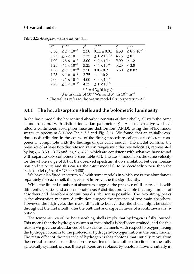
3.4 Variant models 49
Table 3.2: Absorption measure distribution.
ξb f a,b,c ξb f a,b,c ξb f a,b,c
0.50 ≤ 2× 10⁻² 2.50 0.11± 0.01 4.50 ≤ 6× 10⁻³
0.75 ≤ 5× 10⁻⁶ 2.75 ≤ 1× 10⁻¹⁵ 4.75 ≤ 0.11.00 ≤ 5× 10⁻⁴ 3.00 ≤ 2× 10⁻² 5.00 ≥ 1.21.25 ≤ 1× 10⁻³ 3.25 ≤ 4× 10⁻⁸ 5.25 ≤ 3.91.50 ≤ 1× 10⁻¹¹ 3.50 0.8± 0.2 5.50 ≤ 0.021.75 ≤ 1× 10⁻² 3.75 1.1± 0.22.00 ≤ 1× 10⁻¹⁰ 4.00 ≤ 4× 10⁻⁴
2.25 ≤ 1× 10⁻¹⁵ 4.25 ≤ 1× 10⁻³
a f = d NH/d log ξb ξ is in units of 10−9 Wm and NH in 1028 m−2
c The values refer to the warm model fits to spectrum A.3.
3.4.1 The hot absorption shells and the bolometric luminosity
In the basic model the hot ionized absorber consists of three shells, all with the sameabundances, but with distinct ionization parameters ξi. As an alternative we havefitted a continuous absorption measure distribution (AMD), using the SPEX modelwarm, to spectrum A.3 (see Table 3.2 and Fig. 3.6). We found that an initially con-tinuous distribution in the course of the fitting procedure collapses to discrete com-ponents, compatible with the findings of our basic model. The model confirms thepresence of at least two discrete ionization ranges with discrete velocities, representedby log ξ = 3.50− 3.75 and log ξ ≥ 4.75, which are consistent with what we have foundwith separate xabs components (see Table 3.1). The warm model uses the same velocityfor the whole range of ξ, but the observed spectrum shows a relation between ioniza-tion and velocity, and this causes the warm model fit to be decidedly worse than thebasic model (χ2/dof = 17300 / 1480).
We have also fitted spectrum A.3 with some models in which we fit the abundancesseparately for each shell; this does not improve the fits significantly.
While the limited number of absorbers suggests the presence of discrete shells withdifferent velocities and a non-monotonous ξ distribution, we note that any number ofabsorbers and therefore a continuous distribution is possible. The two strong peaksin the absorption measure distribution suggest the presence of two main absorbers.However, the high velocities make difficult to believe that the shells might be stablethroughout the first month after the outburst and argue in favor of a continuous distri-bution.
The temperatures of the hot absorbing shells imply that hydrogen is fully ionized.This means that the hydrogen column of these shells is badly constrained, and for thisreason we give the abundances of the various elements with respect to oxygen, fixingthe hydrogen column to the proto-solar hydrogen-to-oxygen ratio in the basic model.The main effect of the presence of hydrogen is that photons that initially move fromthe central source in our direction are scattered into another direction. In the fullyspherically symmetric case, these photons are replaced by photons moving initially in

50 A phenomenological model for the X-ray spectrum of nova V2491 Cygni
Figure 3.6: Absorption measure distribution (see also Table 3.2).
other directions that are scattered into our direction by Thompson scattering. The slabmodel that we used for the absorbing shell assumes that each photon from the centralsource that is scattered within the shell does not reach the observer, and is not replacedby photons from initially other directions. In the presence of hydrogen, the numberof electrons in the shell is much higher than in the absence of hydrogen, and a muchhigher number of photons is scattered. For a given observed number of photons, theslab model with hydrogen leads to a much higher number of source photons incidenton the shell than the model without hydrogen.
Whether this implementation of the model is valid for V2491 Cyg is not clear. Therapid variations between spectra A.1, A.2 and A.3 may suggest that spherical symme-try does not apply. If spherical symmetry does apply, however, the number of photonsshould not be corrected for scattering, i.e. the luminosity of the central source will bemuch lower than found with the slab model. To investigate the magnitude of this effectwe considered first a variant model in which we set the hydrogen content of the threeshells to zero, but kept the helium. To good approximation, the electron scattering ofthe photons from the central source does not depend on energy within the RGS range,and thus the parameters of the fit are not affected, other than that the luminosity ofthe central source is reduced. In particular, the temperature of the blackbody is thesame as in the basic model. Therefore we computed the luminosity for the blackbodyemitter for the model in which the photon number is not corrected for electron scatter-ing in the absorption shells by fixing all parameters to the values of the basic model,and then recomputed the luminosity of the emitter for spectrum A.3. This luminosity,at 3.92 1031W, and with it the radius, at 3780 km, are much smaller than in the basicmodel.
This reasoning applies equally to a second variant model where we set the hydrogen
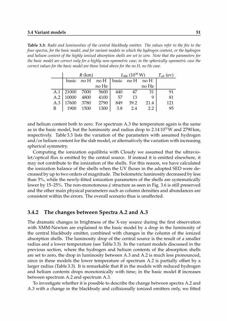
3.4 Variant models 51
Table 3.3: Radii and luminosities of the central blackbody emitter. The values refer to the fits to thefour spectra, for the basic model, and for variant models in which the hydrogen content, or the hydrogenand helium content of the highly ionized absorption shells are set to zero. Note that the parameters forthe basic model are correct only for a highly non-symmetric case; in the spherically symmetric case thecorrect values for the basic model are those listed above for the no H, no He case.
R (km) LBB (1030 W) Teff (ev)basic no H no H basic no H no H
no He no HeA.1 21000 7000 5600 440 47 31 91A.2 10000 4800 4100 57 13 9 81A.3 17600 3780 2790 849 39.2 21.4 121B 1900 1500 1300 3.8 2.4 2.2 95
and helium content both to zero. For spectrum A.3 the temperature again is the sameas in the basic model, but the luminosity and radius drop to 2.14 1031W and 2790 km,respectively. Table 3.3 lists the variation of the parameters with assumed hydrogenand/or helium content for the slab model, or alternatively the variation with increasingspherical symmetry.
Computing the ionization equilibria with Cloudy we assumed that the ultravio-let/optical flux is emitted by the central source. If instead it is emitted elsewhere, itmay not contribute to the ionization of the shells. For this reason, we have calculatedthe ionization balance of the shells when the UV fluxes in the adopted SED were de-creased by up to two orders of magnitude. The bolometric luminosity decreased by lessthan 5%, while the newly-fitted ionization parameters of the shells are systematicallylower by 15–25%. The non-monotonous ξ structure as seen in Fig. 3.6 is still preservedand the other main physical parameters such as column densities and abundances areconsistent within the errors. The overall scenario thus is unaffected.
3.4.2 The changes between Spectra A.2 and A.3
The dramatic changes in brightness of the X-ray source during the first observationwith XMM-Newton are explained in the basic model by a drop in the luminosity ofthe central blackbody emitter, combined with changes in the column of the ionizedabsorption shells. The luminosity drop of the central source is the result of a smallerradius and a lower temperature (see Table 3.3). In the variant models discussed in theprevious section, where the hydrogen and helium contents of the absorption shellsare set to zero, the drop in luminosity between A.3 and A.2 is much less pronounced,since in these models the lower temperature of spectrum A.2 is partially offset by alarger radius (Table 3.3). It is remarkable that R in the models with reduced hydrogenand helium contents drops monotonically with time; in the basic model R increasesbetween spectrum A.2 and spectrum A.3.
To investigate whether it is possible to describe the change between spectra A.2 andA.3 with a change in the blackbody and collisionally ionized emitters only, we fitted
52 A phenomenological model for the X-ray spectrum of nova V2491 Cygni
spectrum A.2 with an alternative model, in which all parameters related to the absorp-tion components were fixed to the values for spectrum A.3, and only the parameters forthe blackbody and for the collisionally ionized plasma were allowed to change. The re-sulting fit is significantly worse (χ2 ≃ 5000, as compared to the best basic fit χ2 ≃ 4000).The χ2 for this fit is dominated by the bad fit to the emission between 25-29 Å, andaround 16 Å.
To investigate whether the lower luminosity may be explained by increased absorp-tion due to increased columns of the ionized shells only, we fit spectrum A.2 with amodel in which the parameters for the central emitters are fixed to the best values ofthe basic model for spectrum A.3, and only the columns and ionization parameters ofthe shells were allowed to vary. The best fit with this variant model has χ2 ≃ 5500,significantly worse than the basic fit for spectrum A.2.
To investigate whether the lower luminosity may be explained by increased absorp-tion due to an increased column of the neutral gas and/or an increased column of thedust, we fit spectrum A.2 with a model in which the columns of the neutral gas and ofthe dust are fitted, but all other parameters were fixed to the best-fit parameters of thebasic model for spectrum A.3. This gives a poor fit, with χ2 ≃ 8000. A model in whichthe central emitter is only partially absorbed by an increased neutral hydrogen columndoes not fit the spectrum at all, because the H I absorption is strongest at λ ∼> 24 Å, apart of the spectrum that remains relatively bright. Therefore, we can exclude absorp-tion by cold clumpy material.
Finally, we have checked whether an addition of a radiative recombination contin-uum (RRC) to the model of spectrum A.2 improves the fit. The presence of this emis-sion is suggested by emission features near 16.8 Å and 18.4 Å. We take into account therecombination of the most relevant ions of took, nitrogen and oxygen. The addition ofRRC to the model does not lead to a significant improvement of the fit.
3.4.3 Derived mass loss rates and model consistency
Our fits to the spectra imply a mass loss rate
Mw =
(
Ω
4π
)
4πr2µmH fc nHv =
(
Ω
4π
)
4πµmHvLξ, (3.2)
where µ is the mean atomic weight in units of the hydrogen mass mH, fc is a factorallowing for clumpiness of the density distribution ( fc ≤ 1), and where Ω = 4π in thecase of spherical symmetry. The observed spectrum gives ξ and v for each shell, almostindependent of L. With the parameters of the standard model fit to spectrum A.3, weobtained the mass loss rates listed in Table 3.4. Note that these values are valid for onetime interval only – i.e. the time of maximum X-ray flux, and thus may overestimatethe outflow-rate averaged over the outburst. From Eq. 3.2 we note in addition that thederived value of Mw scales with the luminosity L of the central source, and thus willbe smaller when the layers are hydrogen- and/or helium-poor (see Table 3), and alsowhen the layers are spherically symmetric, in which case the xabsmodel overestimatesthe central luminosity.
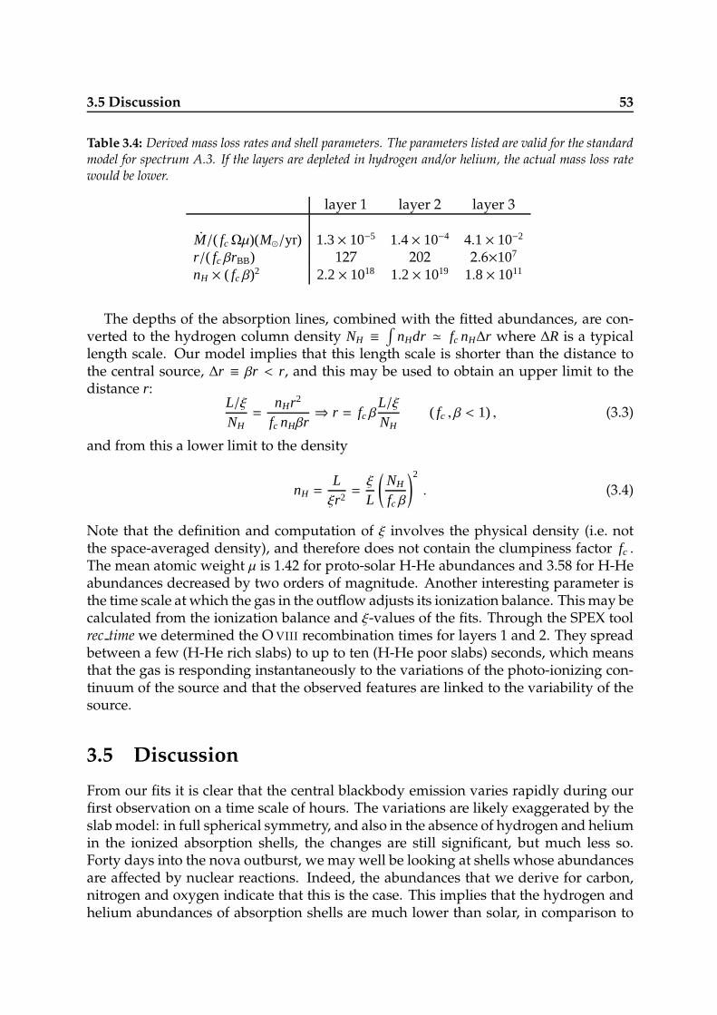
3.5 Discussion 53
Table 3.4: Derived mass loss rates and shell parameters. The parameters listed are valid for the standardmodel for spectrum A.3. If the layers are depleted in hydrogen and/or helium, the actual mass loss ratewould be lower.
layer 1 layer 2 layer 3
M/( fcΩµ)(M⊙/yr) 1.3× 10⁻⁵ 1.4× 10⁻⁴ 4.1× 10⁻²
r/( fc βrBB) 127 202 2.6×10⁷
nH × ( fc β)2 2.2× 10¹⁸ 1.2× 10¹⁹ 1.8× 10¹¹
The depths of the absorption lines, combined with the fitted abundances, are con-verted to the hydrogen column density NH ≡
∫
nHdr ≃ fc nH∆r where ∆R is a typicallength scale. Our model implies that this length scale is shorter than the distance tothe central source, ∆r ≡ βr < r, and this may be used to obtain an upper limit to thedistance r:
L/ξNH=
nHr2
fc nHβr⇒ r = fc β
L/ξNH
( fc , β < 1) , (3.3)
and from this a lower limit to the density
nH =Lξr2=ξ
L
(
NH
fc β
)2
. (3.4)
Note that the definition and computation of ξ involves the physical density (i.e. notthe space-averaged density), and therefore does not contain the clumpiness factor fc .The mean atomic weight µ is 1.42 for proto-solar H-He abundances and 3.58 for H-Heabundances decreased by two orders of magnitude. Another interesting parameter isthe time scale at which the gas in the outflow adjusts its ionization balance. This may becalculated from the ionization balance and ξ-values of the fits. Through the SPEX toolrec time we determined the O VIII recombination times for layers 1 and 2. They spreadbetween a few (H-He rich slabs) to up to ten (H-He poor slabs) seconds, which meansthat the gas is responding instantaneously to the variations of the photo-ionizing con-tinuum of the source and that the observed features are linked to the variability of thesource.
3.5 Discussion
From our fits it is clear that the central blackbody emission varies rapidly during ourfirst observation on a time scale of hours. The variations are likely exaggerated by theslab model: in full spherical symmetry, and also in the absence of hydrogen and heliumin the ionized absorption shells, the changes are still significant, but much less so.Forty days into the nova outburst, we may well be looking at shells whose abundancesare affected by nuclear reactions. Indeed, the abundances that we derive for carbon,nitrogen and oxygen indicate that this is the case. This implies that the hydrogen andhelium abundances of absorption shells are much lower than solar, in comparison to

54 A phenomenological model for the X-ray spectrum of nova V2491 Cygni
the elements just mentioned. Even in the absence of spherical symmetry, therefore, thevariation of the central source is less pronounced than implied by our basic model, andprobably agrees better with the numbers found for the models in which the absorptionshells contain no hydrogen and/or helium.
The response time required for the ionization equilibrium of shells to respond tochanges in the ionizing continuum is a few seconds, which means that the photo-ionization balance of the shells responds almost instantaneously to variations in thesource flux and that its luminosity might indeed have changed. The mass loss ratein our standard model for spectrum A.3 for the third shell in particular is rather highcompared to the common limits 10−4 − 10−3M⊙/yr found for other novae (Kovetz et al.1987; Kato & Hachisu 1989; Smith & Owocki 2006). The derived mass loss rates for allthree layers are lower in the models with reduced hydrogen and/or helium content ofthe absorbing shells.
As discussed in Section 4.1, the blueshifted absorption lines are caused by photonsfrom the central source that initially move in our direction and are scattered into an-other direction. If the dimension of the shell is large with respect to the size of the whitedwarf, and if the optical depth of the shell in the lines is not too high, this will lead to aP Cygni profile, because we see photons initially moving in other directions and thenscattered into our direction in emission, both blue- and red-shifted. The emission andabsorption should have equal strength. In the spectrum of V2491 Cyg this is clearly notthe case. One explanation is that the shell is not large with respect to the white dwarf,so that a large part of the receding half is occulted. Similarly, a high optical depth in theshell may cause photons scattered from the receding half of the shell to be reabsorbedbefore escaping in our direction. And finally, a large asymmetry in the shell may alsoreduce the strength of the redshifted emission.
Carbon and sulfur are about an order of magnitude less abundant than nitrogen andoxygen, and elements such as silicon, argon and calcium are much less abundant. Thissuggests that the white dwarf in V2491 Cyg is an O-Ne and not a C-O white dwarf. Thestrength of the Ne IX-X lines as compared to the C V-VI lines supports this conclusion,as do observations in other wavelength regions (Lynch et al. 2008; Helton et al. 2008;Naik et al. 2009; Munari et al. 2011).
The strongest feature in all X-ray spectra is the rest frame O I K-edge around 23.0 Å,which is well reproduced in the fits together with the corresponding O I 1s-2p absorp-tion line at 23.5 Å. Other features of the cold CSM/ISM are the Fe I L-edge around17.5 Å and the N I 1-2p absorption line at 31.2 Å, both well fitted by our models. Neu-tral oxygen and nitrogen are highly overabundant, whereas iron is slightly overabun-dant, with respect to solar abundances. This suggests that part of the cold absorptionoriginates in enriched circumstellar matter close to V2491 Cyg. The reduction of thecolumn and the decrease in temperature of the cold absorber between spectra A.1 andB suggests that the CSM column is mostly derived from the current nova outburst,and still expanding, albeit slowly. Page et al. (2010a) suggested that the reduction ofthe column stops at 2.2×1025 m−2 some time after our second observation. This finalvalue then corresponds to the interstellar component. If the total O I column is equallydivided between CSM and ISM, the ISM may have a near-solar abundance for oxygen,and sub-solar abundance for iron, implying that iron is depleted by dust.
3.6 Conclusions and prospects 55
The optical flux defines the nova outburst, and thus clearly must come from theexpanding nova envelope; the ultraviolet flux changes in tandem with the optical flux,and therefore also originates from the nova envelope. As can be seen from Fig. 3.5, ourmodel fails to predict the correct level of the ultraviolet and optical fluxes by severalorders of magnitude. This indicates that our model applies only, if at all, to the X-raypart of the spectrum, which must originate from a very different layer in the expandingenvelope, presumably much closer to the white dwarf than the layers responsible forthe optical/ultraviolet spectrum. This conclusion is confirmed by the observation thatthe marked changes in the X-ray flux during the first XMM-Newton observation arenot accompanied by changes in the optical and/or ultraviolet fluxes.
Because the absorption lines from the shells are shifted from the rest wavelengths bythe high outflow velocities, and because hot atmospheres do not show deep absorptionlines even at the rest wavelengths using a blackbody spectrum as the central source isnot as poor choice as might appear at first sight. As a first test we have tried a model at-mosphere spectrum that replaces the blackbody as the central source. Following Nesset al. (2011) we used the best fitting TMAP model of Rauch & Werner (2010) (007, withlog g = 9 and T = 106 K). This provides an even worse fit with χ2 = 15 with three shells,18 with two shells, 32 with just one shell and 59 without any photo-ionized absorber(instead of 7 from the BB fit) because O VIII / N VII line ratio (the most important inthe spectrum) cannot be reproduced by the atmosphere model. It may be necessaryto consider models with different abundances and outflows which, however, are cur-rently not available and we therefore refrain from a systematic parameter study of theatmosphere model parameters.
3.6 Conclusions and prospects
Our spectral analysis of nova V2491 Cyg suggests that the absorption by highly-ion-ized ions is caused by non-monotonous, possibly discrete, ejecta shells with differentoutflow velocities and ionization levels. Variations on time scales of hours occur bothin the luminosity of the central source and in the ionization level and columns of theabsorption shells. We find that in our scenario of photo-ionization equilibrium theexpanding gas is responding almost instantaneously to the variations in the sourceionizing continuum. Our upper limits for the mass loss rate of each shell agree withthose estimated for other novae, especially if the shells are depleted in hydrogen.
The values derived from the fits for the luminosity and radius of the central sourcedepend on the nature of the models that are applied, and therefore must be considereduncertain. In the spherically symmetric case, however, the radius of the central emitterof X-rays decreases monotonically with time, and therefore must be in the increasinglytransparent expanding nova envelope. The values derived for the abundances in theionized absorption shells do not depend on the details of the models, and thereforemay be considered more secure. These abundances indicate that the white dwarf inV2491 Cyg is an O-Ne white dwarf.
Improvements to our pilot models can be made in several ways. First, it would beuseful to replace the central blackbody emitter with an appropriate white-dwarf at-
56 A phenomenological model for the X-ray spectrum of nova V2491 Cygni
mosphere model. We have tested a model in which the TMAP model substitutes theblackbody, but is still absorbed by the three shells. However, this model provides evenpoorer results than those obtained with our standard fits with a blackbody continuum.In the future atmosphere models must take into account different abundances and out-flows.
Second, it will be necessary to iterate between the computation of the ionizationstructure of the ionizing shells for a given spectral energy distribution, and the com-putation of the spectral energy distribution and elemental abundances from the fit, foreach of the four observed spectra separately. For this improvement it is also necessaryto determine the distance more reliably: a close distance implies a lower luminosityand thereby a lower ionization parameter of the shells. Finally, it would be usefulto obtain constraints on the hydrogen contents of the hot ionized absorption shells,perhaps from ultraviolet observations. Ultraviolet observations may also help in de-termining the location of origin of the optical/ultraviolet flux.
Acknowledgements
This work is based on observations obtained with XMM-Newton, an ESA science mis-sion with instruments and contributions directly funded by ESA Member States andthe USA (NASA). SRON is supported financially by NWO, the Netherlands Organiza-tion for Scientific Research. We also acknowledge financial support from the Facultyof the European Space Astronomy Centre. We also thank the referee for importantsuggestions, which improved the quality of the paper.
Chapter 4
Multiwavelength campaign on Mrk 509IX. The Galactic foreground
C. Pinto1, G. A. Kriss2,3, J. S. Kaastra1,4, E. Costantini1, J. Ebrero1, K. C. Steenbrugge5,6,M. Mehdipour7, G. Ponti8
1 SRON Netherlands Institute for Space Research, Utrecht, The Netherlands2 Space Telescope Science Institute, Baltimore, USA3 Department of Physics and Astronomy, Johns Hopkins University, Baltimore, USA4 Astronomical Institute, Utrecht University, Utrecht, The Netherlands5 Instituto de Astronomia, Universidad Catolica del Norte, Antofagasta, Chile6 Department of Physics, University of Oxford, Oxford, UK7 Mullard Space Science Laboratory, University College London, Surrey, UK8 School of Physics and Astronomy, University of Southampton, Southampton, UK
Received 19 December 2011 / Accepted 22 March 2012
Published in Astronomy & Astrophysics, volume 541, pages A147–165, 2012
Abstract
The diffuse gas in and nearby the Milky Way plays an important role in the evolu-tion of the entire Galaxy. It has a complex structure characterized by neutral, weaklyand highly ionized gas, dust, and molecules. We probe this gas through the obser-vation of its absorption lines in the high-energy spectra of background sources. We
58 Multiwavelength campaign on Mrk 509 IX. The Galactic foreground
use high-quality spectra of AGN Mrk 509, located at high Galactic latitudes obtainedwith XMM-Newton, HST and FUSE. We use advanced absorption models consistingof photo- and collisional-ionization. We constrain the column density ratios of the dif-ferent phases of the interstellar medium (ISM) and measure the abundances of C, N, O,Ne, Mg, Al, Si, S, and Fe. We detect seven discrete interstellar clouds with different ve-locities. One is a typical low-velocity cloud (LVC) and three belong to the family of theintermediate-velocity clouds (IVCs) found near the Galactic disk. These four cloudsshow large deviation from Solar abundances in the gas phase, mostly caused by dustdepletion. The other three clouds are ionized high-velocity clouds (HVCs) and are lo-cated either in the Galactic environment or in the Local Group halo as suggested by thesignatures of collisional ionization. The similar abundances and ionization structure ofthe HVCs suggest a common location and origin: they might belong to the remainderof an extragalactic cloud which was captured by the Galaxy.We have shown that com-bined UV / X-ray spectroscopy is a powerful tool to investigate the ISM. In commonGalactic clouds, like LVCs and IVCs, the ISM shows a complex structure consisting ofat least three different temperature phases.
4.1 Introduction
The interstellar medium (ISM) drives the evolution of the Galaxy: it is enriched withheavy elements during the course of stellar evolution, and it also provides the sourceof material for the subsequent star formation. In the spectra of background sources theISM gives rise to reddening and absorption lines. The ISM shows a clear multi-phasestructure (for a review, see Ferriere 2001). The cold phase is a blend of dust, moleculesand gas below 104 K. The warm ionized gas is weakly ionized, with a temperature of∼ 104 K. The hot ionized gas is characterized by temperatures of about 106 K.
The multi-phase medium plays an important role in the evolution of the Galaxy.One of the parameters that affect the stellar evolution is the metallicity of the starforming regions. Stellar winds and supernovae expel part of the interstellar gas outof the Galactic disk, but gravity generally stops the gas from escaping, such that itfalls back through the process known as ”Galactic fountain” (Shapiro & Field 1976).Gas accreted from smaller galaxies, e.g. the Magellanic Clouds, and the intergalacticmedium increases the reservoir of low metallicity gas. High-velocity clouds (HVCs)play a crucial role in this process.
HVCs contain neutral hydrogen at velocities incompatible with a simple model ofdifferential Galactic rotation. In practice one uses a Local Standard of Rest veloc-ity VLSR ≥ 90 km s−1 to define HVCs (for a review see Wakker & van Woerden 1997).ISM absorbers with 30 . VLSR . 90 km s−1 are usually defined as intermediate-velocityclouds (IVCs). Both IVCs and HVCs might originate from our Galaxy or have an ex-ternal origin. They could be debris from Galactic fountains or infalling Local Groupgas (Blitz et al. 1999). Of course, a Galactic fountain origin would imply metallicitiesnear solar, while infall from the Local Group or the intergalactic medium (IGM) wouldimply metal poor gas. The presence of infalling matter is required in order to maintainstar formation in the Galaxy: without a substantial replenishing of the gas available
4.1 Introduction 59
the star formation would stop in a period much shorter than the Hubble Time. HVCsare thought to contain enough mass to sustain star formation rate (SFR) in the Galaxy(Lehner & Howk 2011).
A multiwavelength approach provides the means to analyze the ISM in a completeway. For instance, combined UV and X-ray spectroscopy provides accurate columndensities and the velocity structure of the most abundant ionic species. Ionic specieslike Si II-IV, C II-IV, N V and O VI especially, are quite common in HVCs (Sembach et al.2003). In the last decade interstellar absorption lines in UV spectra of background starshave provided the distances of several IVCs and HVCs (see e.g. Richter 2006; Lehner &Howk 2011, and references therein). In summary, all the main H I complexes are knownto be Galactic. IVCs are at typical distances of . 2kpc, while HVCs with 90 . VLSR .
170 km s−1 are found between 4–13 kpc. No cloud is found at VLSR ≥ 170 km s−1 towardshalo stars, while several of them are found towards AGNs, which suggests that thesevery-high velocity clouds (VHVCs) are at larger distances. However all are thought tobe within 40 kpc (Richter 2006), except the Magellanic Stream which is at about 50 kpc,much closer than the typical distances in the Local Group halo. A plausible scenario isthat VHVCs are the next generation of HVCs infalling towards the Galactic disk andslowing down during their interaction with it (Lehner & Howk 2011).
The AGN Mrk 509 has been intensively studied for both its intrinsic spectral fea-tures and its interesting line-of-sight. The Galactic latitude for Mrk 509 is –30 degreesand crosses the halo of our Galaxy, resulting in an important contribution of ionizedgas. First evidence for ionized gas was found by York et al. (1982), who discoveredsignificant absorption from Si II, Fe II and C IV in the spectra taken with the IUE satel-lite. They also observed strong Lyα absorption as well as red-shifted lines from Ca II
and Na II in optical spectra. Blades & Morton (1983) attributed these shifted lines tocorotating gas in our halo. This was confirmed by the detection of neutral hydrogenwith VLSR ∼ 60 km s−1 (McGee & Newton 1986). Sembach et al. (1995) and Sembachet al. (1999) discovered two sets of lines of Si III-IV and C IV with large velocities, i.e.VLSR ∼ −230 km s−1 and −280 km s−1, which were attributed to absorption by HVCs.Sembach et al. (2003) argued that these clouds are photo-ionized by the extra-Galacticbackground, but the presence in large quantities of hot gas such as O VI cannot be ex-plained by the photo-ionization models and suggests that these clouds are probablyinteracting with the hot Galactic corona or the Local Group medium. To explain theionized C, Si and O column densities Collins et al. (2004) concluded that the HVCshave multiple phases. They showed that the Si III-IV and C IV can be produced by aQSO photo-ionizing background, while the O VI indicates collisional ionization due tothe interaction with the Galactic corona. We note that the presence of molecular H2 inthe LOS (Wakker 2006) affects the spectral region near the O VI UV line and its columndensity estimate.
More than fifteen years after the discovery of these HVCs, their structure is not yetwell understood. To solve these questions improved collisional and photo-ionizationmodels are needed to constrain the ionization processes occurring in HVCs, as wellas a multiwavelength approach which uses all the available archival data in order toincrease the number of ions detected as well as the ionization parameter range that wecan sample, and to disentangle the molecular H2 and the O VI absorption.
60 Multiwavelength campaign on Mrk 509 IX. The Galactic foreground
This article is one of a series of papers analyzing the deep and broad multiwave-length campaign on Mrk 509. The overview of the campaign is presented in Kaastraet al. (2011b), hereafter paper I. Here we present the analysis of the interstellar cloudsin the LOS towards Mrk 509 through a combined UV / X-ray analysis of the spec-tra taken with the Hubble Space Telescope / Cosmic Origin Spectrograph (HST/COS)(Green et al. 2012) and the XMM-Newton Reflection Grating Spectrometer (RGS, denHerder et al. 2001). Our analysis is focused on both the LVC, IVCs and HVCs and thedust present along the LOS towards Mrk 509. We constrain velocity, ionization andchemical structure of the ISM for the different ionic species.
The paper is organized as follows. In Sect. 5.2 we present the data. In Sect. 5.3we report the relevant spectral features that we analyze. In Sect. 5.4 we describe themodels we use and the results of our analysis. The discussion and the comparison withprevious work are given in Sect. 5.5. Conclusions are reported in Sect. 5.6.
4.2 The data
As part of our multiwavelength campaign we observed Mrk 509 in the far-ultravioletwavelength band between 1155 Å and 1760 Å using the Far-Ultraviolet Channel andthe medium resolution gratings of the Cosmic Origins Spectrograph (COS) onboardthe Hubble Space Telescope (HST). A detailed explanation of the observing strategy,instrument performance, data reduction, and calibration can be found in Kriss et al.(2011), hereafter paper VI. They also present a full-scale plot of the high-resolutionspectrum.
To summarize the data briefly, the observations were taken on 2009 December 10and 11 simultaneously with the Chandra LETGS observations in our campaign (Ebreroet al. 2011). Using the COS gratings G130M and G160M, we obtained total exposuretimes of 9470 s and 16452 s, respectively. With each grating, we used only two differentgrating tilts with a single FP-POS for each to avoid creating gaps in the spectral regionsof interest including the AGN outflow features. The data were processed with theCOS calibration pipeline v2.11b at STScI. With central wavelengths of 1309 and 1327for G130M, 1577 and 1589 for G160M, and two exposures at each tilt, we obtained asufficient variety of independent placements of the spectrum on the detector to identifyinstrumental features in our high signal-to-noise spectrum. Known features such asdead spots were excluded from the combined data; correctable features such as grid-wire shadows were removed via a customized flat-field treatment described by Krisset al. (2011). Kriss et al. (2011) also describe improved wavelength calibration appliedto the data. Finally, they deconvolved the spectra using a Lucy-Richardson algorithmto remove the effects of the broad wings of the COS line-spread function (Ghavamianet al. 2009; Kriss 2011). This correction is essential to recover the true depths of narrowinterstellar absorption lines; comparison to prior STIS spectra of Mrk 509 validatesthe effectiveness of the deconvolution. We use the original spectrum to identify weakspectral features, while we use the deconvolved spectrum for measuring the depth andwidth of identified absorption lines.
For the X-ray portion of our study we use the stacked XMM-Newton RGS spectrum
4.3 Spectral features 61
of Mrk 509 that consists of ten ∼60 ks individual observations. The observations anddata reduction for this stacked RGS spectrum are described by Kaastra et al. (2011a),hereafter paper II. Briefly, they used the SAS 9.0 software package to reduce the tenindividual observations. They then created a fluxed spectrum for each observationand stacked these, using RGS 1 and 2 and both spectral orders, and taking the effectsof the XMM-Newton multi-pointing mode into account.
In addition to the COS and RGS spectra, we also use an archival spectrum obtainedwith the Far Ultraviolet Spectroscopic Explorer (FUSE) for the O VI 1032 Åabsorption line.The FUSE data are described in paper VI.
For our spectral analysis we use SPEX1 version 2.03.00 (Kaastra et al. 1996). SPEXis a software package optimized for the analysis and interpretation of high-resolutionUV and X-ray spectra. In SPEX one can simultaneously use different components forcontinuum emission as well as absorption by photo-ionized or collisionally-ionizedgas (see the SPEX manual). We scale elemental abundances to the proto-Solar valuesrecently recommended by Lodders & Palme (2009). We use a linear scale for the abun-dances. Throughout this paper we use SI units which are also the units system used inour spectral codes, adopt 1σ errors, and use χ2 statistics unless otherwise stated. Wedefine high-ionization ions to be more than four times ionized, like O VI-VIII, whilesingle to four times ionized ions are defined as low / intermediate-ionization ions, ascommonly done in X-ray spectroscopy.
4.3 Spectral features
4.3.1 The COS spectrum
Most features in the COS spectrum are foreground absorption lines due to the ISM ofthe Galaxy. We detected absorption lines from seven discrete ISM components (seeTable 7, paper VI). We also found three absorption lines due to the diffuse intergalacticmedium in the LOS towards the AGN. In Figs. 4.1, 4.2 and 4.3 we plot the prominentinterstellar lines present in the COS spectrum. The lines are sorted according to theirionization state and ionization potential. All lines are plotted in velocity space andin units of normalized flux. The zero-velocity of the scale is given by the laboratorywavelength of each transition. For consistency and easy comparison with previouswork we then convert velocities to the Local Standard of Rest (LSR). The conversionfrom the laboratory to the LSR scale is given by vLSR =vLab + 11.16km s−1 (Blades &Morton 1983).
In the COS spectrum the ISM features are resonance lines and encompass up to 5ionization states, e.g. from N I to N V. The strongest lines are the N I triplet around1200 Å, the O I line at 1302 Å, and the Fe II and Al II lines at 1608.4 and 1670.8 Å, re-spectively. Multiple strong transitions from both Si II and S II are shown, as well asC IV and Si IV doublets. The C II and Si III lines are heavily saturated. We confirm thepresence of several discrete absorbers, seven in the case of C IV as found in paper VI,
1www.sron.nl/spex

62 Multiwavelength campaign on Mrk 509 IX. The Galactic foreground
00.
51
C I 1277.2 Å
AB CD E F G
00.
51
N I 1200.7 Å(Triplet)
1200.21199.5
A B C D E F G
00.
51
C I 1328.8 Å
00.
51
O I 1302.2 Å
00.
51
Nor
mal
ilzed
Flu
x
C I 1560.3 Å0
0.5
1
Nor
mal
ilzed
Flu
xAl II 1670.8 Å
−400 −200 0 200 400
00.
51
V LSR (km s−1)
C I 1656.9 Å
−400 −200 0 200 400
00.
51
V LSR (km s−1)
Fe II 1608.4 Å
Figure 4.1: HST/COS absorption lines from the cold phase (ionization states I-II). The flux is normalizedto the continuum emission and the lines are displayed in the Local Standard of Rest system. The restframe wavelength of each resonance line is also given. The dotted lines represent the average velocities ofthe seven cloud systems (Kriss et al. 2011), which are also labeled as A to G.
with vLSR of about -295, -240, -125, -65, +5, +65 and +90 to +130 km s−1. We label theseabsorbers with alphabetical letters ranging from A to G and sort them according totheir vLSR (Table 4.1). Moreover, we adopt the standard nomenclature for the clouds:the absorbers that produce components A, B and C are HVCs as their velocity modulusis greater than 100 km s−1. The absorbers responsible for components D, F, and G areintermediate velocity clouds (IVC). Component E is a low-velocity cloud (LVC).
4.3.2 The FUSE spectrum
FUSE observed Mrk 509 in 1999 for about 52 ks (Kriss et al. 2000) and in 2000 for 62.1 ks(paper VI). We use only the last observation because of its higher S/N ratio. We use theFUSE spectrum mostly for the analysis of the absorption lines due to the interstellarO VI (see Fig. 4.5).
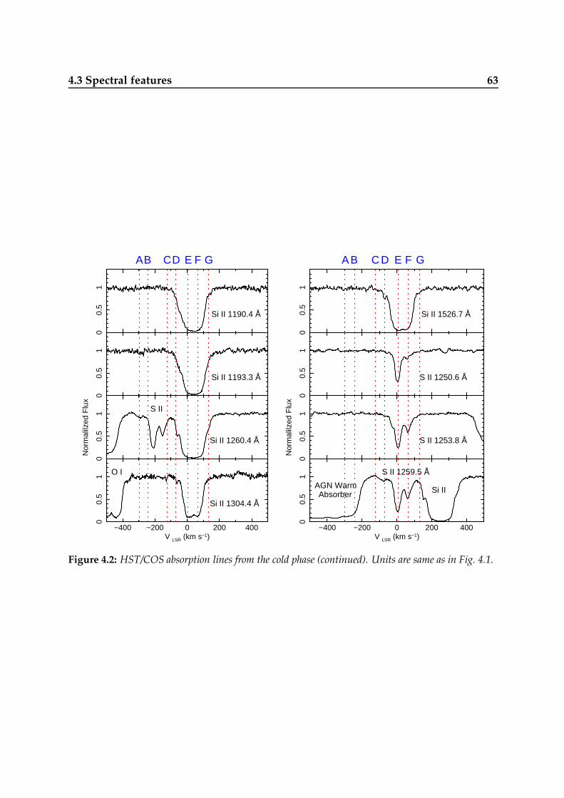
4.3 Spectral features 63
00.
51
Si II 1190.4 Å
AB CD E F G
00.
51
Si II 1526.7 Å
A B C D E F G
00.
51
Si II 1193.3 Å
00.
51
S II 1250.6 Å
00.
51
Nor
mal
ilzed
Flu
x
Si II 1260.4 Å
S II
00.
51
Nor
mal
ilzed
Flu
x
S II 1253.8 Å
−400 −200 0 200 400
00.
51
V LSR (km s−1)
Si II 1304.4 Å
O I
−400 −200 0 200 400
00.
51
V LSR (km s−1)
Si II
S II 1259.5 Å
AGN WarmAbsorber
Figure 4.2: HST/COS absorption lines from the cold phase (continued). Units are same as in Fig. 4.1.

64 Multiwavelength campaign on Mrk 509 IX. The Galactic foreground
00.
51
C II 1334.5 Å
HVC C II*
AB CD E F G
00.
51
C IV 1548.2 Å
HVC HVC (1550)
A B C D E F G
00.
51
Si III 1206.5 Å
HVC
00.
51
C IV 1550.8 Å
HVC
00.
51
Nor
mal
ilzed
Flu
x
Si IV 1393.8 ÅHVC
00.
51
Nor
mal
ilzed
Flu
x
N V 1238.8 Å
Mg II Mg II
+ IGMHVC
−400 −200 0 200 400
00.
51
V LSR (km s−1)
Si IV 1402.8 ÅHVC
−400 −200 0 200 400
00.
51
V LSR (km s−1)
N V 1242.8 Å
HVC
Figure 4.3: HST/COS absorption lines from the warm phase (ionization states III-V). Units are sameas in Fig. 4.1.
4.4 Spectral modeling of the ISM 65
4.3.3 The RGS spectrum
The XMM-Newton RGS spectrum of Mrk 509 is complex because most of the observedfeatures are intrinsic to the AGN and some of them blend with foreground absorptionlines as shown in paper II. Absorption and emission lines intrinsic to the AGN canbe distinguished from the ISM lines as the former are significantly red-shifted. For acomplete analysis of the AGN intrinsic absorption we refer to Detmers et al. (2011),hereafter paper III. The strongest ISM features are the O I and N I absorption lines at23.5 Å and 31.3 Å, respectively. Clear evidence of highly ionized gas is provided bythe O VII-VIII lines at 21.6 and 19.0 Å. We plot the individual RGS absorption edges ofneutral O, Fe, and N together with the most prominent high-ionization lines in Fig. 4.7.
4.4 Spectral modeling of the ISM
Our analysis focuses on the absorption lines of the ISM along the LOS towards Mrk 509.These lines are narrower than the features intrinsic to the AGN and always narrowerthan 1 Å. The only exception is the H I Lyα absorption line at 1215.67 Å, which hasa FWHM of 20 Å (see Fig. 4.4). In order to reproduce both the AGN continuum andnarrow and broad emission lines, we use the continuum emission model of paper VI.The spectral ranges that are strongly affected by intrinsic absorption were excludedas the AGN analysis is carried in other paper (Kriss et al. 2011). For the RGS spectralmodeling we used the continuum plus line emission model (Model 2) given in paper IIIfor the warm absorber. First we analyze the ISM in the UV and in the X-rays separatelydue to the different resolution of the instruments. The different velocity componentsare resolved in the UV spectra (see Fig. 4.1, 4.2 and 4.3), but this it is not yet possible inthe X-ray band.
4.4.1 UV spectral fits
We have performed the UV analysis in two steps. First, we use an empirical modelto estimate the velocity shift and dispersion of each absorption line and the ionic col-umn density. This model provides information on the significance and kinematics ofall the components. It further gives hints of their ionization state and location withinthe Galaxy. In the second method we use physical models to provide a more realisticdescription of the several foreground absorbers. These models provide important in-formation on the ionization state, abundances and the sources responsible for heatingthe ISM. A final simultaneous fit to the UV and X-ray spectra was performed to obtainrobust results by covering the entire range of ionization states.
An empirical slab model for the COS–UV spectra
The first ISM model we use consists of seven slab components, which are required inorder to reproduce the 7 different kinematic ISM absorbers observed in the COS andFUSE spectra. Only C IV clearly shows all seven components (see Fig. 4.3). Excluding
66 Multiwavelength campaign on Mrk 509 IX. The Galactic foreground
C II, the low-ionization absorption lines require no more than four components. Thuslow-ionization gas is not detected for the HVCs. The slab model in SPEX calculatesthe transmission of a slab of material, where all ionic column densities can be chosenindependently. This has the advantage that the spectrum can be fitted without anyprior knowledge of the ionization balance. The slab model jointly fits all the lines thatare are produced by the same ion. After an acceptable spectral fit is obtained, we cancompare the observed column densities with those predicted from photo-ionizationmodels. Free parameters in the slab model are the velocity dispersion σv, the Dopplervelocity shift v and the ionic column density NX .
For some UV saturated lines there is a degeneracy between the velocity dispersionand column density, hence the determined column density is uncertain. For severalions we only detect saturated lines in the UV spectrum, thus we have performed si-multaneous fits for lines with similar ionization potential, like H I, N I and Mg II (seeFig. 4.4), tying their v and σv. All lines of the same ion were simultaneously fitted likethe four C I lines (see Fig. 4.1), the five Si II and three S II lines (see Fig. 4.2), as well asthe Si IV, C IV and N V doublets (see Fig. 4.3). In order to simplify our model and toshorten the CPU time we force the component A, B and C (HVCs) to have the samevelocity dispersion, and similarly for components E, F and G (IVCs, see Table 4.1). Apreliminary fit to the strong, resolved lines of N I, Fe II, S II, C IV and S IV did give con-sistent values for the velocity dispersion σv within these groups. Only component Dshows a rather smaller σv, thus we treat it separately. In the cases where componentD was too weak or blended, we froze σv to the value obtained for O I, the strongestline in component D. The N V 1238.8 Å line is affected by IGM absorption (paper VI)and the O VI HVC lines are affected by the presence of molecular H2 (Wakker 2006).To reproduce the IGM line we added a slab of H I with v = 5700 km s−1, σv = 40 km s−1
and very small column density logNH i = 17.2 m−2 in agreement with paper VI. TwoGaussians were added to model the H2 absorption at 1031.2 Å. These Gaussians havevelocity shifts of +3 and +60 km s−1, σv = 8 km s−1, and equivalent widths of 0.06 and0.03 Å, respectively in agreement with Wakker (2006). Thus, both the N V and O VI col-umn densities, as given in Table 4.1, are corrected by IGM and H2 contamination. TheC II absorption lines appear to be different from the other low-ionization ions like S II
and Si II. Among the low ions, only C II clearly shows high-velocity absorption. More-over, a separate fit of the C II and C I absorption lines provides a column density ratioC II/C I ∼ 100and a velocity dispersion ratio σC ii/σC i > 3, which are inconsistent withthe other column density ratios of low ions like O I-II and N I-II. This suggests that thebulk of the neutral carbon in the cold phase is depleted into dust grains and that mostof the C II is provided by the warm phase as confirmed by our physical models (seeSect. 4.4.2.) For these reasons we prefer to fit the C II absorption lines together with theintermediate ions. We empirically model the H I absorption assuming that it is all inthe cold phase. Our physical model confirms that the the neutral hydrogen present inthe cold phase is indeed two orders of magnitude larger than that in the warm and hotphases.
In Figs. 4.4 and 4.5 we show the data and best fit models for the most prominent linesof the cold, warm and hot ISM phases. The results of the best fit with the seven slabcomponents are reported in Table 4.1. They are sorted according to the velocity shift

4.4 Spectral modeling of the ISM 67
(columns) and ionization potential (rows). We also group the ions which have beenfitted together: H I, N I and Mg II; Si II and Al II; Fe II and Ni II; C II-IV, Si III-IV and N V.We generally detect low-ionization lines only for the LVC and IVCs (components E andD, F and G), thus four slab components are sufficient to model these low-intermediatevelocity absorbers. However, we need seven slab components for modeling the mildlyionized gas providing the bulk of C II and all two or more times ionized ions. We notethat the σv on average increases with the ionization state. A comparison of the columndensities of the three HVCs (component A to C) shows that the fastest component A isthe least ionized.
In order to simultaneously fit the absorption lines of the mildly ionized gas, we ap-plied a few wavelength shifts to certain ions to match both the IVC and HVC features.These shifts are likely due to residual errors in the COS and FUSE wavelength cali-bration. We applied no shift for both C IV and Si IV as their profiles perfectly match(see Fig. 4.5). The Si III lines have been shifted by −8 km s−1, the C II and N V lines by−10 km s−1. We also shifted the FUSE O VI lines by −14.5 km s−1 to obtain a match withthe COS C IV HVC lines. Because the O VI features are blended and affected by H2
absorption, in the spectral fits we prefer to fix all the O VI LOS velocities to those of theC IV and S II lines, which are well constrained.
A physical analysis of the interstellar absorbers requires more realistic models. Inthe next subsection we test two different SPEX models to reproduce both the neutraland ionized gas phases: the hot and the xabs models, which reproduce collisional andphoto-ionization respectively.
A collisionally-ionized model for the cold gas
The hot model in SPEX calculates the transmission of a collisionally-ionized equilib-rium (CIE) plasma. For a given temperature and set of abundances, the model calcu-lates the ionization balance and then determines all the ionic column densities by scal-ing to the prescribed total hydrogen column density. At low temperatures this modelmimics the neutral interstellar gas (see SPEX manual and Kaastra et al. 2009). Free pa-rameters in the hot model are the hydrogen column density NH, the temperature T , thevelocity dispersion σv and shift v and the abundances.
Following the ISM analysis of Pinto et al. (2010), we have first modeled the cold gaswith a low-temperature collisionally-ionized gas. The interstellar cold gas is responsi-ble for the low ionization absorption lines: H I, C I, N I, O I, Mg II, Al II, Si II, S II, Ni II,and Fe II. These lines arise from the LVC and IVCs (components D-G) and no signif-icant low-ionization absorption is detected at high outflow velocities (see Table 4.1).Thus, we modeled the cold gas with just four CIE components, one for the LVC andthree for the IVCs. As previously assumed for the slab model, we take the same σv
for the three reddest absorbers, E-F-G. We also adopted the same abundances for com-ponents D to G: the poor statistics and the line blending give degenerate fits that donot allow us to constrain the abundances of these four absorbers separately. For thestrongest components E and F we performed a fit with decoupled abundances for S,Fe and N. The abundances of both components were consistent within the errors.
At first we assumed proto-Solar abundances. The fit was not satisfactory for any

68 Multiwavelength campaign on Mrk 509 IX. The Galactic foreground
Table 4.1: Spectral fits to the COS and FUSE spectra using the empirical model with 7 slab components.Dashes are non detections.
A (a) B (a) C (a) D (a) E (a) F (a) G (a)
σ (b) — — — ≡ 2.0 (e) 4.5± 0.4
v (b) — — — −50± 10 −1± 1 62± 1 100± 10
C I (c) — — — 15.7± 0.3 17.6± 0.1 16.8± 0.1 16.2± 0.1
σ (b) < 10(d) — — 2.0± 0.4 9± 1
v (b) −290± 5 — — −64± 1 +7± 3 71± 5 131± 10
O I (c) > 16.4 (d) — — 19.2± 0.4 21.1± 0.2 20.7± 0.1 17.1± 0.1
σ (b) — — — ≡ 2.0 (e) 7.5± 0.5
v (b) — — — −64± 5 +8± 2 70± 1 100± 5
H I (c) — — — — 24.53± 0.02 23.2± 0.1 —
N I (c) — — — 16.4± 0.4 19.5± 0.2 18.6± 0.1 17.4± 0.1
Mg II (c) — — — 18.1± 0.1 19.8± 0.1 18.6± 0.3 18.2± 0.1
σ (b) < 4 (d) — — ≡ 2.0 (e) 13± 1
v (b) −300± 10 — — −65± 5 5± 5 65± 5 131± 10
Si II (c) 16.7± 0.2 — — 17.9± 0.3 19.5± 0.4 19.4± 0.2 16.8± 0.3
Al II (c) 16± 1 — — 17.3± 0.1 18.2± 0.1 17.5± 0.2 15.5± 0.5
σ (b) < 7.6 (d) — — 1.1± 0.4 7.3± 0.3
v (b) −300± 5 — — −72.1± 0.3 2.8± 0.2 58± 1 89± 1
Fe II (c) > 16.7 (d) — — 17.5± 0.1 19.3± 0.1 18.47± 0.05 17.56± 0.03
Ni II (c) — — — 16.7± 0.2 17.53± 0.02 17.30± 0.03 16.93± 0.07
σ (b) — — — 3.6± 0.6 6.4± 0.7
v (b) — — — −71.4± 0.3 4.9± 0.1 61.7± 0.5 89± 2
S II (c) — — — 17.7± 0.1 20.6± 0.1 18.78± 0.02 17.8± 0.1
σ (b) 12.0± 0.2 2.6± 0.6 18± 1
v (b) −297.6± 0.2 −244± 1 −124± 3 −69± 1 6± 1 66± 2 132± 5
C II (c) 17.62± 0.03 17.0± 0.1 < 16.4 (d) 19.2± 0.5 20.00± 0.05 19.10± 0.05 17.4± 0.1
Si III (c) 17.53± 0.02 16.59± 0.03 15.8± 0.2 16.0± 0.1 19.01± 0.05 18.40± 0.06 16.5± 0.1
Si IV (c) 17.34± 0.01 16.35± 0.07 15.6± 0.3 15.9± 0.2 17.70± 0.01 17.43± 0.01 15.9± 0.1
C IV (c) 18.26± 0.01 17.52± 0.02 16.7± 0.2 16.6± 0.2 18.34± 0.01 18.14± 0.01 16.9± 0.1
N V (c) 16.7± 0.1 16.5± 0.2 < 16.2 (d) 16.5± 0.2 17.30± 0.07 17.2± 0.1 < 16.7 (d)
σ (b) 14± 2 6± 4 40± 6
v (b) ≡ −297.6 (e) ≡ −244(e) ≡ −124(e) ≡ −69(e) ≡ 6 (e) ≡ 66(e) ≡ 132(e)
O VI(c) 17.6± 0.1 17.74± 0.05 17.5± 0.1 16.2± 0.2 18.25± 0.03 18.34± 0.08 17.3± 0.1
(a) The different slab components.(b) Both the velocity dispersion σ and the LSR v are in units of km s−1.(c) The ionic column densities NX are in log (m−2) units.(d) 2σ lower / upper limits, respectively.(e) Fixed parameters.

4.4 Spectral modeling of the ISM 69
NH (χ2ν > 10) due to the over-predicted ionic column densities: C I ∼ 3 × 10²⁰ m−2, Si I
∼ 4×10¹⁸ m−2 and Mg II ∼ 2.4×10²⁰ m−2. The column densities as measured for both C I
and Mg II using the fit with the empirical slab models are much lower (see Table 4.1)and the Si I lines are not detected in the spectrum.
A fit with free abundances provides only a partial improvements and the main prob-lems are the high Si II/Si I and C II/C I column density ratios. These ratios can be re-
−2000 −1000 0 1000 2000
00.
20.
40.
60.
81
Nor
mal
ized
Flu
x
HI 1215.7
IGM
−400 −200 0 200
00.
20.
40.
60.
81
NI 1200.7
−100 0 100 200
0.8
0.9
1
V LSR (km s−1)
MgII 1239.9
Figure 4.4: Best fit to the HST/COS absorption lines of the cold gas with the slab model (see alsoTable 4.1).
70 Multiwavelength campaign on Mrk 509 IX. The Galactic foreground
produced only through the combined effect of a high gas temperature and depletiononto dust. A satisfactory fit is reached when we assume that at least 80% of Mg and90% of C and Si are depleted from the gaseous phase into dust grains.
The weakly ionized gas of the LVC and IVCs shows rather high temperatures ofabout 15 000–20 000 K as expected by the significant S II column density and the ab-sence of S I (which cannot be attributed to depletion into dust). This suggests that animportant fraction of hydrogen is ionized. Component E, the one at rest, provides 90%of the total NH i, while component F is the second strongest but accounts for only ∼ 5%.The measured σv are consistent with those estimated through the slab model. The H I
column densities measured by the two different models are consistent with each other,but their total H I column is only about 75% of the value measured at 21 cm (Murphyet al. 1996), which might be due to the high saturation of the UV line or most likely tothe difference in beam-size between the 21 cm radio observation and the pencil-beamUV observation. Because the O I 1302.2 Å line is heavily saturated, it is difficult to mea-sure the oxygen abundance. Thus we freeze it to the proto-Solar value. For a completeanalysis of the abundances we refer to Sect. 4.4.2, in which we fit the entire UV / X-raydataset. We have also tested an alternative photo-ionization model for the cold gas andobtained similar results (see Sect. 5.5.1).
A photo-ionized model for the warm ionized gas
To model the warm (mildly) ionized gas responsible for the C II-IV and Si III-IV ab-sorption observed in all velocity components, we tried a collisional ionization model.However, it is not possible to obtain a satisfactory fit with seven collisionally-ionizedgas components for any of the HVCs (A to C) and LVC / IVCs (D to G). This is be-cause collisional ionization results in a narrow peak in ionization, while a wide rangeof ionization states is observed. An alternative solution might be multi-phase CIE gas,which we have tested without obtaining satisfactory results (see Sect. 5.5.1), or cool-ing gas out of ionization equilibrium (see e.g. Gnat & Sternberg 2007). Here we use aphoto-ionization model for the mildly ionized gas, which provides a good solution.
For the photo-ionization modeling we use the xabs model in SPEX. The xabs modelcalculates the transmission of a slab of material, where all ionic column densities arelinked through a photo-ionization model. The relevant parameter is the ionization pa-rameter ξ = L/nr2, with L the source ionizing luminosity between 1 − 1000Ryd, n thedensity and r the distance from the ionizing source. Free parameters in the xabs modelare the hydrogen column density NH, the ionization parameter ξ, the velocity disper-sion σv, the Doppler velocity shift v, and the abundances. We have created a modelconsisting of seven photo-ionized xabs components, one for each velocity componentdetected. Similar to the slab and hot models, we have coupled the σv and abundanceswithin the two LVC / IVC and HVC groups (see Sect. 4.4.1 and Fig. 4.5), i.e. compo-nents A-B-C and E-F-G.
The spectral energy distribution (SED) plays a crucial role in determining the ion-ization balance in the photo-ionized layers (see e.g. Chakravorty et al. 2009). Unfortu-nately, the SED which determines the ionization balance of the interstellar gas is notwell known. For this reason, we have tested different SEDs on the seven ISM absorbers

4.4 Spectral modeling of the ISM 71
−400 −200 0 200
00.
51
CII 1334.5
−400 −200 0 200
00.
51
SiIII 1206.5
−400 −200 0 200
0.4
0.6
0.8
1
Nor
mal
ized
Flu
x
SiIV 1402.8
−400 −200 0 200
00.
51
CIV 1548.2
−400 −200 0 200
0.6
0.8
1
V LSR (km s−1)
NV 1238.8
IGM
−400 −200 0 200
0.2
0.4
0.6
0.8
1
V LSR (km s−1)
OVI 1031.9
H2
Figure 4.5: Simultaneous fit to the HST/COS and FUSE warm and hot gas components with the slabmodel (see also Table 4.1).
(see also Fig. 4.6):
1. local emissivity (LE) of all the galaxies and QSOs, i.e. the integrated emission ofgalaxies and QSOs as seen in the local Universe at z = 0;
2. local emissivity (at z = 0) of only QSOs;
3. cosmic background radiation plus X-ray background as measured by HEAO1and BeppoSAX;
4. interstellar field SED (entirely due to starlight);
5. powerlaw (PL) SEDs.
The first three SEDs represent a purely extragalactic ionizing source and have beentaken from Haardt & Madau (2001, 2012). The interstellar field SED refers to the onespecified in the CLOUDY ”Hazy” manual (Ferland 2005). For the last case (SED 5) wehave created a grid of powerlaw SEDs (Fν ∝ να) with slopes ranging from −4.0 to −0.1

72 Multiwavelength campaign on Mrk 509 IX. The Galactic foreground
Figure 4.6: SEDs which have been used in the fit of the warm photo-ionized gas. Arbitrary units areused in order to compare the shape of the SEDs. LE SED refers to QSO + galaxies. See also Sect. 4.4.1.
with steps of 0.05 and with a low-energy cut-off below 1 Ryd. We calculate the ion-ization balance through the SPEX xabsinput tool: it receives as input the ionizing SEDand the abundances of the gas, and determines the ionization balance using Cloudyversion 08.00 (see the SPEX manual for more details).We have used the normalizationfor the physical SEDs as given in the literature, but we note that the absolute normal-ization of the SED does not matter while the SED shape does (see e.g. Sect. 6.2 in theSPEX manual). In order to have a sufficiently broad energy band, xabsinput adds aminimum flux value at energies of 10−8 and 109 Ryd, which does not affect the results.Because we do not know the abundances a priori, we have decided to fix them to theproto-Solar values of Lodders & Palme (2009). We have adopted the same SED andabundances for the IVC group, and similarly for the HVC group. This choice is sug-gested by the fact that large deviations in ionization balance and metallicity are mostlyexpected by comparing LVC / IVCs lying in the Galactic disk with the halo HVCs (seebelow).
Among the four physically motivated SEDs, only the local emissivity (LE) SED in-cluding galaxies plus QSOs provides a satisfactory fit with proto-Solar abundances(χν ∼ 1.3, see Table 4.2) for all seven absorbers. The other physical SEDs do not providegood fits even when allowing for highly non-solar abundances. The powerlaw SEDsprovide results similar to the best fitting LE SED. For absorption from both IVCs andHVCs the best fit is obtained by assuming a PL SED with slope α ∼ −2, and proto-Solar abundances. The main difference between the PL and LE SEDs are the derivedξ values. The ionization parameters are systematically higher for a LE SED (see Table
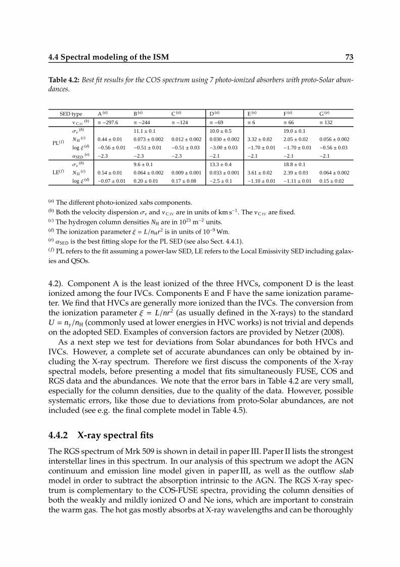
4.4 Spectral modeling of the ISM 73
Table 4.2: Best fit results for the COS spectrum using 7 photo-ionized absorbers with proto-Solar abun-dances.
SED type A (a) B (a) C (a) D (a) E (a) F (a) G (a)
v C iv
(b) ≡ −297.6 ≡ −244 ≡ −124 ≡ −69 ≡ 6 ≡ 66 ≡ 132
PL( f )
σv(b) 11.1± 0.1 10.0± 0.5 19.0± 0.1
N H(c) 0.44± 0.01 0.073± 0.002 0.012± 0.002 0.030± 0.002 3.32± 0.02 2.05± 0.02 0.056± 0.002
log ξ (d) −0.56± 0.01 −0.51± 0.01 −0.51± 0.03 −3.00± 0.03 −1.70± 0.01 −1.70± 0.01 −0.56± 0.03
αSED(e) −2.3 −2.3 −2.3 −2.1 −2.1 −2.1 −2.1
LE( f )
σv(b) 9.6± 0.1 13.3± 0.4 18.8± 0.1
N H(c) 0.54± 0.01 0.064± 0.002 0.009± 0.001 0.033± 0.001 3.61± 0.02 2.39± 0.03 0.064± 0.002
log ξ (d) −0.07± 0.01 0.20± 0.01 0.17± 0.08 −2.5± 0.1 −1.10± 0.01 −1.11± 0.01 0.15± 0.02
(a) The different photo-ionized xabs components.(b) Both the velocity dispersion σv and v C iv are in units of km s−1. The v C iv are fixed.(c) The hydrogen column densities NH are in 1023 m−2 units.(d) The ionization parameter ξ = L/nHr2 is in units of 10−9 Wm.(e) αSED is the best fitting slope for the PL SED (see also Sect. 4.4.1).( f ) PL refers to the fit assuming a power-law SED, LE refers to the Local Emissivity SED including galax-
ies and QSOs.
4.2). Component A is the least ionized of the three HVCs, component D is the leastionized among the four IVCs. Components E and F have the same ionization parame-ter. We find that HVCs are generally more ionized than the IVCs. The conversion fromthe ionization parameter ξ = L/nr2 (as usually defined in the X-rays) to the standardU = nγ/nH (commonly used at lower energies in HVC works) is not trivial and dependson the adopted SED. Examples of conversion factors are provided by Netzer (2008).
As a next step we test for deviations from Solar abundances for both HVCs andIVCs. However, a complete set of accurate abundances can only be obtained by in-cluding the X-ray spectrum. Therefore we first discuss the components of the X-rayspectral models, before presenting a model that fits simultaneously FUSE, COS andRGS data and the abundances. We note that the error bars in Table 4.2 are very small,especially for the column densities, due to the quality of the data. However, possiblesystematic errors, like those due to deviations from proto-Solar abundances, are notincluded (see e.g. the final complete model in Table 4.5).
4.4.2 X-ray spectral fits
The RGS spectrum of Mrk 509 is shown in detail in paper III. Paper II lists the strongestinterstellar lines in this spectrum. In our analysis of this spectrum we adopt the AGNcontinuum and emission line model given in paper III, as well as the outflow slabmodel in order to subtract the absorption intrinsic to the AGN. The RGS X-ray spec-trum is complementary to the COS-FUSE spectra, providing the column densities ofboth the weakly and mildly ionized O and Ne ions, which are important to constrainthe warm gas. The hot gas mostly absorbs at X-ray wavelengths and can be thoroughly
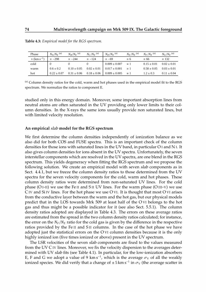
74 Multiwavelength campaign on Mrk 509 IX. The Galactic foreground
Table 4.3: Empirical model for the RGS spectrum.
Phase NA/NE(a) NB/NE
(a) NC/NE(a) ND/NE
(a) NE/NE(a) NF/NE
(a) NG/NE(a)
v (km s−1) ≡ −298 ≡ −244 ≡ −124 ≡ −69 ≡ 6 ≡ 66 ≡ 132
cold 0 0 0 0.009± 0.007 ≡ 1 0.15± 0.01 0.02± 0.01
warm 0.6± 0.2 0.10± 0.05 0.02± 0.01 0.017± 0.001 ≡ 1 0.58± 0.05 0.03± 0.01
hot 0.22± 0.07 0.31± 0.06 0.18± 0.06 0.009± 0.005 ≡ 1 1.2± 0.3 0.11± 0.04
(a) Column density ratios for the cold, warm and hot phases used in the empirical model fit to the RGS
spectrum. We normalize the ratios to component E.
studied only in this energy domain. Moreover, some important absorption lines fromneutral atoms are often saturated in the UV providing only lower limits to their col-umn densities. In the X-rays the same ions usually provide non saturated lines, butwith limited velocity resolution.
An empirical slab model for the RGS spectrum
We first determine the column densities independently of ionization balance as wealso did for both COS and FUSE spectra. This is an important check of the columndensities for those ions with saturated lines in the UV band, in particular O I and N I. Italso gives column densities for ions absent in the UV spectra. Unfortunately, the seveninterstellar components which are resolved in the UV spectra, are one blend in the RGSspectrum. This yields degeneracy when fitting the RGS spectrum and we propose thefollowing solution. We create an empirical model with seven slab components as inSect. 4.4.1, but we freeze the column density ratios to those determined from the UVspectra for the seven velocity components for the cold, warm and hot phases. Thesecolumn density ratios were determined from non-saturated UV lines. For the coldphase (O I-II) we use the Fe II and S II UV lines. For the warm phase (O III-V) we useC IV and Si IV lines. For the hot phase we use O VI. It is thought that most O VI arisesfrom the conductive layer between the warm and the hot gas, but our physical modelspredict that in the LOS towards Mrk 509 at least half of the O VI belongs to the hotgas and thus might be a possible indicator for it (see also Sect. 5.5.1). The columndensity ratios adopted are displayed in Table 4.3. The errors on these average ratiosare estimated from the spread in the two column density ratios calculated; for instance,the error on the NF/NE ratio for the cold gas is given by the difference in the respectiveratios provided by the Fe II and S II columns. In the case of the hot phase we haveadopted just the statistical errors on the O VI column densities because it is the onlyhighly ionized ion (five times ionized or above) present in the UV spectrum.
The LSR velocities of the seven slab components are fixed to the values measuredfrom the UV C IV lines. Moreover, we fix the velocity dispersion to the averages deter-mined with UV slab fits (see Table 4.1). In particular, for the low-ionization absorbersE, F and G we adopt a value of 9 km s−1, which is the average σV of all the weaklyionized species. We did verify that a change of ± 5km s−1 in σV (the average scatter in
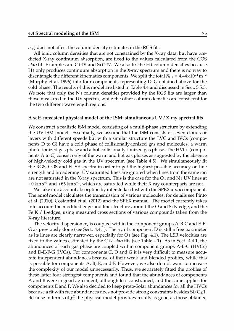
4.4 Spectral modeling of the ISM 75
σV) does not affect the column density estimates in the RGS fits.All ionic column densities that are not constrained by the X-ray data, but have pre-
dicted X-ray continuum absorption, are fixed to the values calculated from the COSslab fit. Examples are C I-IV and Si II-IV. We also fix the H I column densities becauseH I only produces continuum absorption in the X-ray spectrum and there is no way todisentangle the different kinematics components. We split the total NH i = 4.44×1024 m−2
(Murphy et al. 1996) into four components representing D–G obtained above for thecold phase. The results of this model are listed in Table 4.4 and discussed in Sect. 5.5.3.We note that only the N I column densities provided by the RGS fits are larger thanthose measured in the UV spectra, while the other column densities are consistent forthe two different wavelength regions.
A self-consistent physical model of the ISM: simultaneous UV / X-ray spectral fits
We construct a realistic ISM model consisting of a multi-phase structure by extendingthe UV ISM model. Essentially, we assume that the ISM consists of seven clouds orlayers with different speeds but with a similar structure the LVC and IVCs (compo-nents D to G) have a cold phase of collisionally-ionized gas and molecules, a warmphoto-ionized gas phase and a hot collisionally-ionized gas phase. The HVCs (compo-nents A to C) consist only of the warm and hot gas phases as suggested by the absenceof high-velocity cold gas in the UV spectrum (see Table 4.5). We simultaneously fitthe RGS, COS and FUSE spectra in order to get the highest possible accuracy on linestrength and broadening. UV saturated lines are ignored when lines from the same ionare not saturated in the X-ray spectrum. This is the case for the O I and N I UV lines at+0km s−1 and +65km s−1, which are saturated while their X-ray counterparts are not.
We take into account absorption by interstellar dust with the SPEX amol component.The amol model calculates the transmission of various molecules, for details see Pintoet al. (2010); Costantini et al. (2012) and the SPEX manual. The model currently takesinto account the modified edge and line structure around the O and Si K-edge, and theFe K / L-edges, using measured cross sections of various compounds taken from theX-ray literature.
The velocity dispersion σv is coupled within the component groups A-B-C and E-F-G as previously done (see Sect. 4.4.1). The σv of component D is still a free parameteras its lines are clearly narrower, especially for O I (see Fig. 4.1). The LSR velocities arefixed to the values estimated by the C IV slab fits (see Table 4.1). As in Sect. 4.4.1, theabundances of each gas phase are coupled within component groups A-B-C (HVCs)and D-E-F-G (IVCs). For components C, D and G it is very difficult to measure accu-rate independent abundances because of their weak and blended profiles, while thisis possible for components A, B, E, and F. However, we also do not want to increasethe complexity of our model unnecessarily. Thus, we separately fitted the profiles ofthese latter four strongest components and found that the abundances of componentsA and B were in good agreement, although less constrained, and the same applies forcomponents E and F. We also decided to keep proto-Solar abundances for all the HVCsbecause a fit with free abundances does not provide strong constraints besides Si/C&1.Because in terms of χ2
ν the physical model provides results as good as those obtained
76 Multiwavelength campaign on Mrk 509 IX. The Galactic foreground
Table 4.4: RGS spectral fits: empirical model with 7 slab absorbers. All the units are same as inTable 4.1.
Par A B C D E F G
v ≡ −298 ≡ −244 ≡ −124 ≡ −69 ≡ 6 ≡ 66 ≡ 132
σ — — — ≡ 2.0 ≡ 9
H I — — — ≡ 22.2 ≡ 24.6 ≡ 23.6 ≡ 22.6
N I — — — 18.3 20.27± 0.06 19.5 18.6
N II — — — 16.7 18.5± 0.5 17.8 17.0
O I — — — 19.2 21.4± 0.1 20.5 19.6
O II — — — 17.9 19.8± 0.3 19.0 18.2
Ne I — — — 18.6 20.7± 0.1 19.9 19.0
Ne II — — — < 18.4 < 20.4 < 19.6 < 18.7
Mg I — — — < 18.7 < 20.7 < 19.9 < 19.0
Mg II — — — < 18.7 < 20.7 < 19.9 < 19.0
Fe I — — — 17.8 19.7± 0.3 18.9 18.1
Fe II — — — < 17.8 < 19.8 < 19.0 < 18.1
σ ≡ 12 ≡ 2.6 ≡ 18
C V 18.9 18.1 17.4 17.3 19.1± 0.3 18.9 17.5
O III 19.2 18.4 17.6 17.6 19.5± 0.2 19.2 17.8
O IV 19.0 18.2 17.5 17.4 19.3± 0.3 19.0 17.6
Ne III 19.8 18.9 18.1 18.1 20.0± 0.2 19.7 18.3
σ ≡ 14 ≡ 6 ≡ 40
C VI 18.5 18.7 18.5 17.1 19.2± 0.1 19.3 18.2
N VI 18.3 18.5 18.2 16.9 19.0± 0.1 19.1 18.0
N VII 18.2 18.3 18.1 16.8 18.9± 0.3 19.0 17.9
O VI 18.2 18.3 18.1 16.8 18.9± 0.3 19.0 17.9
O VII 19.4 19.6 19.3 17.9 20.14± 0.05 20.2 19.1
O VIII 19.0 19.1 18.9 17.5 19.7± 0.1 19.8 18.6
Ne IX 18.9 19.0 18.8 17.4 19.6± 0.2 19.7 18.6
Ne X 18.5 18.7 18.4 17.0 19.2± 0.5 19.3 18.2
Fe XVII 16.6 16.7 16.5 15.3 17.2± 0.2 17.3 16.3
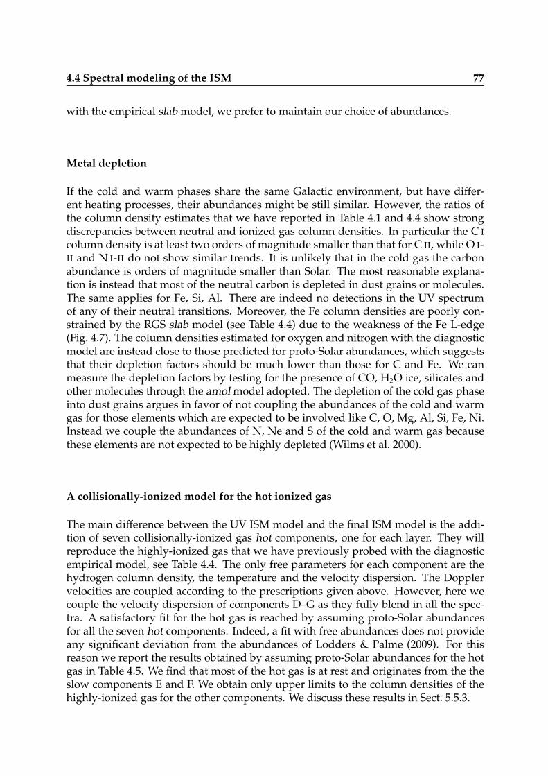
4.4 Spectral modeling of the ISM 77
with the empirical slab model, we prefer to maintain our choice of abundances.
Metal depletion
If the cold and warm phases share the same Galactic environment, but have differ-ent heating processes, their abundances might be still similar. However, the ratios ofthe column density estimates that we have reported in Table 4.1 and 4.4 show strongdiscrepancies between neutral and ionized gas column densities. In particular the C I
column density is at least two orders of magnitude smaller than that for C II, while O I-II and N I-II do not show similar trends. It is unlikely that in the cold gas the carbonabundance is orders of magnitude smaller than Solar. The most reasonable explana-tion is instead that most of the neutral carbon is depleted in dust grains or molecules.The same applies for Fe, Si, Al. There are indeed no detections in the UV spectrumof any of their neutral transitions. Moreover, the Fe column densities are poorly con-strained by the RGS slab model (see Table 4.4) due to the weakness of the Fe L-edge(Fig. 4.7). The column densities estimated for oxygen and nitrogen with the diagnosticmodel are instead close to those predicted for proto-Solar abundances, which suggeststhat their depletion factors should be much lower than those for C and Fe. We canmeasure the depletion factors by testing for the presence of CO, H2O ice, silicates andother molecules through the amol model adopted. The depletion of the cold gas phaseinto dust grains argues in favor of not coupling the abundances of the cold and warmgas for those elements which are expected to be involved like C, O, Mg, Al, Si, Fe, Ni.Instead we couple the abundances of N, Ne and S of the cold and warm gas becausethese elements are not expected to be highly depleted (Wilms et al. 2000).
A collisionally-ionized model for the hot ionized gas
The main difference between the UV ISM model and the final ISM model is the addi-tion of seven collisionally-ionized gas hot components, one for each layer. They willreproduce the highly-ionized gas that we have previously probed with the diagnosticempirical model, see Table 4.4. The only free parameters for each component are thehydrogen column density, the temperature and the velocity dispersion. The Dopplervelocities are coupled according to the prescriptions given above. However, here wecouple the velocity dispersion of components D–G as they fully blend in all the spec-tra. A satisfactory fit for the hot gas is reached by assuming proto-Solar abundancesfor all the seven hot components. Indeed, a fit with free abundances does not provideany significant deviation from the abundances of Lodders & Palme (2009). For thisreason we report the results obtained by assuming proto-Solar abundances for the hotgas in Table 4.5. We find that most of the hot gas is at rest and originates from the theslow components E and F. We obtain only upper limits to the column densities of thehighly-ionized gas for the other components. We discuss these results in Sect. 5.5.3.
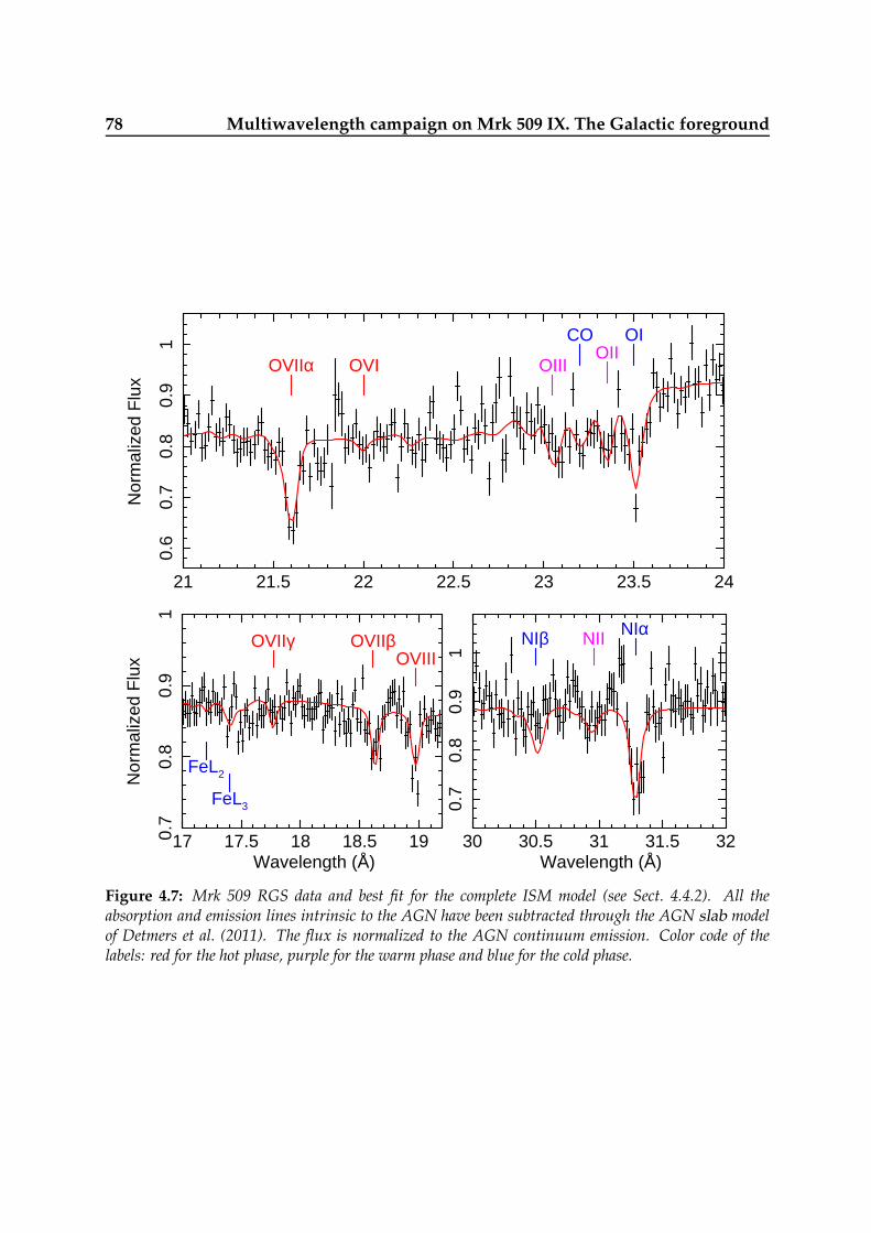
78 Multiwavelength campaign on Mrk 509 IX. The Galactic foreground
21 21.5 22 22.5 23 23.5 24
0.6
0.7
0.8
0.9
1
Nor
mal
ized
Flu
x
OVIIα OVI OIII
COOII
OI
17 17.5 18 18.5 190.7
0.8
0.9
1
Nor
mal
ized
Flu
x
Wavelength (Å)
FeL3
OVIIγ OVIIβOVIII
FeL2
30 30.5 31 31.5 32
0.7
0.8
0.9
1
Wavelength (Å)
NIβ NII NIα
Figure 4.7: Mrk 509 RGS data and best fit for the complete ISM model (see Sect. 4.4.2). All theabsorption and emission lines intrinsic to the AGN have been subtracted through the AGN slab modelof Detmers et al. (2011). The flux is normalized to the AGN continuum emission. Color code of thelabels: red for the hot phase, purple for the warm phase and blue for the cold phase.

4.4 Spectral modeling of the ISM 79
Table 4.5: UV / X-ray simultaneous fits with the final complete ISM model.
Phase Par A B C D E F G
v (a) ≡ −297.6 ≡ −244 ≡ −124 ≡ −69 ≡ 6 ≡ 66 ≡ 132
Cold gas
σv(a) — — — < 2 9.6± 0.1
NH(b) — — — 0.9± 0.1 44± 1 8± 1 0.09± 0.04
T (eV) — — — < 0.6 1.26± 0.01 1.24± 0.02 2.7± 0.1
C/H (c) — — — < 0.1
N/H (c) — — — 0.8± 0.1
O/H (c) — — — 0.5± 0.1
Ne/H (c) — — — 1.3± 0.1
Mg/H (c) — — — 0.41± 0.04
Al/H (c) — — — 0.06± 0.01
Si/H (c) — — — 0.14± 0.04
S/H (c) — — — 0.67± 0.01
Fe/H (c) — — — 0.07± 0.01
Ni/H (c) — — — 0.07± 0.01
Warm gas
σv(a) 9.8± 0.1 4.7± 0.2 18.5± 0.1
NH(b) 0.52± 0.01 0.065± 0.002 0.010± 0.002 0.034± 0.002 5.4± 0.3 2.9± 0.1 0.013± 0.002
logξ (b) −0.03± 0.01 0.17± 0.01 0.22± 0.08 −2.3± 0.2 −1.13± 0.01 −1.12± 0.01 0.7± 0.2
C/H (c) ≡ 1 ≡ 1
O/H (c) ≡ 1 0.5± 0.1
Al/H (c) ≡ 1 0.33± 0.08
Si/H (c) ≡ 1 0.60± 0.01
Fe/H (c) ≡ 1 0.90± 0.06
Hot gas
σv(a) < 11 16± 6
NH(b) < 0.3 < 0.4 < 0.5 1.7± 0.5 19± 3 4± 1 < 1
T (eV) 40± 10 55± 15 51± 14 14± 1 160± 10 70± 10 55± 15
Molecules
CO (d) — — — — 7.5± 1.5 — —
H2O ice (d) — — — — < 1.0 — —
MgSiO3(d) — — — — < 0.8 — —
Fe (d) — — — — < 0.6 — —
Fe2O3(d) — — — — < 0.3 — —
H2(d, e) — — — — 10− 50 4− 6 —
(a) Velocity units are same as in Table 4.1. Doppler velocities v are fixed.(b) The hydrogen column densities NH are in units of 1023 m−2. The ionization parameter ξ is in units of
10−9 Wm.(c) Abundances ratios are in the linear proto-Solar abundance units of Lodders & Palme (2009).(d) Molecular column densities are in units of 1020 m−2.(e) H2 column densities are taken from Wakker (2006).
80 Multiwavelength campaign on Mrk 509 IX. The Galactic foreground
4.4.3 Alternative models
In this section we report several tests to check the validity and uniqueness of ourmodel.
The first issue concerns the physical state of the cold weakly ionized gas. We haveused a collisionally-ionized model in SPEX because at low temperatures this mimicswell the cold interstellar gas (see Sect. 4.4.1). However, at these temperatures photo-ionization could also provide a significant contribution. Thus, we tried an alternativemodel in which four additional photo-ionized xabs components (E to G) substitute forthe cold collisionally-ionized ones. The fit slightly worsens and absolute abundances,i.e. relative to hydrogen, are not well constrained. They show systematic deviationsof about 25–50% from the values obtained with the collisionally-ionized model, whileabundances relative to oxygen or other well constrained ions have smaller deviations.In summary, a photo-ionized plasma provides a worse fit to the cold phase, but inprinciple part of the cold component might be photo-ionized.
Excluding C II, ions like O I-II and O III-IV have been put in two different phasesin the slab model (see Sect. 4.4.1). Although the physical model takes into accountcontributions to each ion from any phase, we have to justify the choice adopted forthe empirical slab model. At first we chose to fit the C II together with the C IV andSi III-IV because it was the only ‘low’ ion clearly showing high-velocity absorption. Thephysical model validates this choice as most of the carbon in the cold phase turns out tobe locked into dust and the bulk of C II comes from the warm photo-ionized phase. Forcompleteness we have tested a photo-ionization model for each velocity componentin order to fit the entire set of neutral to doubly ionized ions (and ignoring all theother lines), assuming they are from a warm weakly-ionized phase and decoupledfrom the remaining more highly ionized ions. However, the fit is worse than before(∆χ2
ν ∼ +1.0); the observed C II/C I, Si II/Si III and S II/S III column density ratios arenot well reproduced. Even if we add dust depletion for carbon and silicon we cannotobtain satisfactory results (at any NH).
We have also considered an alternative interpretation of the warm mildly-ionizedgas that produces most of C III-IV and Si III-IV. Instead of seven photo-ionized ab-sorbers (see Sect. 4.4.1) we used multiphase collisionally-ionized gas: each velocitycomponent has been fitted with 2 or even 3 CIE components. This model provides theworst fit so far. It might be that the gas is out of equilibrium, but we cannot check thisfurther with the current spectral models in SPEX. However, the goodness of fit of ourstandard model suggests that photo-ionization is a likely interpretation.
The last important issue concerns O VI. We have so far considered this ion, togetherwith O VII-VIII, as a tracer of the hot highly-ionized gas. However, as we have previ-ously mentioned in Sect. 4.4.2, most of O VI is thought to arise from a cooling colderphase with temperatures 1 − 5 × 10⁵ K (see e.g. Richter 2006). Therefore, we have ap-plied a collisionally-ionized model for this conductive phase that produces N V andO VI assuming a temperature of 2.1 − 4.4 × 10⁻² keV (2.5 − 5.1 × 10⁵ K). However, thismodel is incompatible with another collisionally-ionized phase producing O VII-VIII.In order to explain the O VIII/O VII and Ne X/Ne IX ratios this highest-ionization gasalso provides at least half of the observed O VI. In summary, either half of the O VI is
4.5 Discussion 81
contained in the hot ionized gas, or a significant amount of O VII belongs to the cool-ing intermediate phase. In both cases there is a link between the column densities ofthe O VI-VII ions. For this reason we prefer our standard model and fit together allhighly-ionized ions including and exceeding those five times ionized, like O VI.
4.5 Discussion
Our analysis shows that the ISM in the LOS of Mrk 509 has a multi-phase structure (seeTable 4.1 and 4.5) and complex dynamics. The ISM structure is similar for the differentvelocities components A–G, but the LVC and IVCs show a three-phase structure whilethe HVCs show only two ionized phases. We first discuss the general structure of theISM that we have probed, its constituents and chemistry. Then, we will characterizethe several absorbers, describe their heating processes and locate them in the Galacticenvironment.
4.5.1 ISM multi-phase structure
In the LOS towards Mrk 509 the ISM is found in different physical and chemical forms.We found the gas at various temperatures with different heating processes. Our UVspectral modeling has revealed a large sample of ionization states (see Table 4.1) whichis further enlarged by including the X-ray detected absorption. The velocity dispersionis the same within clouds which belong to the same family, such as the IVCs. We haveindeed obtained a very good fit by coupling the velocity dispersion of the LVC andIVC components E, F, and G (see Figs. 4.4 and 4.5). Component D is an exception.
The cold phase
We have successfully modeled the interstellar gas with three main phases (see Ta-ble 4.5). For the cold gas we have used a collisionally-ionized gas with low temper-atures kT ∼ 0.5− 2.7eV (6 000− 30 000K). It provides the bulk of the neutral and low-ionization lines, such as O I-II, N I-II, Fe I-II and S II. We detect the cold gas only for theLVC and IVCs, no neutral gas is found at high speed (see Table 4.1). More than 90% ofthe neutral gas is provided by the LVC component E. Component F (VLSR = 65 km s−1)is the second in order of column density and has an ionization state consistent with theLVC (for both the cold and warm gas), which suggests a similar environment for thetwo clouds.
In Sect. 4.4.1 we have already shown that the C I column densities are too low withrespect to those of O I and N I for the C I / C II ratio to be explained only by heating ofthe cold gas phase. We also argued that at least 90% of C and Si from the cold phaseis locked into molecules and dust grains. We confirm this with the complete physicalmodel detailed in Table 4.5. We have indeed obtained a 2σ upper limit of 0.1 for boththe carbon and silicon abundances with respect to the proto-Solar value of Lodders &Palme (2009). This strongly suggests the presence of both carbonaceous and silicatecompounds in the LOS. We have thus tested all the molecules available in the SPEX
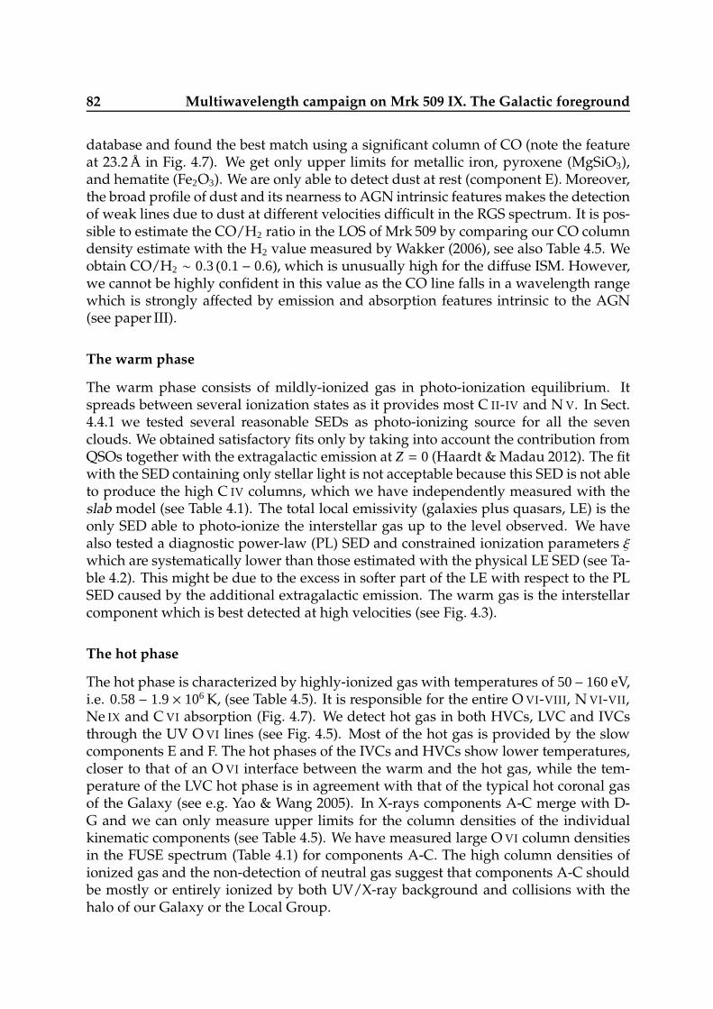
82 Multiwavelength campaign on Mrk 509 IX. The Galactic foreground
database and found the best match using a significant column of CO (note the featureat 23.2 Å in Fig. 4.7). We get only upper limits for metallic iron, pyroxene (MgSiO3),and hematite (Fe2O3). We are only able to detect dust at rest (component E). Moreover,the broad profile of dust and its nearness to AGN intrinsic features makes the detectionof weak lines due to dust at different velocities difficult in the RGS spectrum. It is pos-sible to estimate the CO/H2 ratio in the LOS of Mrk 509 by comparing our CO columndensity estimate with the H2 value measured by Wakker (2006), see also Table 4.5. Weobtain CO/H2 ∼ 0.3 (0.1− 0.6), which is unusually high for the diffuse ISM. However,we cannot be highly confident in this value as the CO line falls in a wavelength rangewhich is strongly affected by emission and absorption features intrinsic to the AGN(see paper III).
The warm phase
The warm phase consists of mildly-ionized gas in photo-ionization equilibrium. Itspreads between several ionization states as it provides most C II-IV and N V. In Sect.4.4.1 we tested several reasonable SEDs as photo-ionizing source for all the sevenclouds. We obtained satisfactory fits only by taking into account the contribution fromQSOs together with the extragalactic emission at Z = 0 (Haardt & Madau 2012). The fitwith the SED containing only stellar light is not acceptable because this SED is not ableto produce the high C IV columns, which we have independently measured with theslab model (see Table 4.1). The total local emissivity (galaxies plus quasars, LE) is theonly SED able to photo-ionize the interstellar gas up to the level observed. We havealso tested a diagnostic power-law (PL) SED and constrained ionization parameters ξwhich are systematically lower than those estimated with the physical LE SED (see Ta-ble 4.2). This might be due to the excess in softer part of the LE with respect to the PLSED caused by the additional extragalactic emission. The warm gas is the interstellarcomponent which is best detected at high velocities (see Fig. 4.3).
The hot phase
The hot phase is characterized by highly-ionized gas with temperatures of 50− 160eV,i.e. 0.58− 1.9× 10⁶ K, (see Table 4.5). It is responsible for the entire O VI-VIII, N VI-VII,Ne IX and C VI absorption (Fig. 4.7). We detect hot gas in both HVCs, LVC and IVCsthrough the UV O VI lines (see Fig. 4.5). Most of the hot gas is provided by the slowcomponents E and F. The hot phases of the IVCs and HVCs show lower temperatures,closer to that of an O VI interface between the warm and the hot gas, while the tem-perature of the LVC hot phase is in agreement with that of the typical hot coronal gasof the Galaxy (see e.g. Yao & Wang 2005). In X-rays components A-C merge with D-G and we can only measure upper limits for the column densities of the individualkinematic components (see Table 4.5). We have measured large O VI column densitiesin the FUSE spectrum (Table 4.1) for components A-C. The high column densities ofionized gas and the non-detection of neutral gas suggest that components A-C shouldbe mostly or entirely ionized by both UV/X-ray background and collisions with thehalo of our Galaxy or the Local Group.

4.5 Discussion 83
In order to estimate the location of the hot gas of components E and F we performa test on the 620 ks MOS 1-2 data (paper I). We selected an annular region between10-12’ around Mrk 509 in both the MOS detectors and obtained their spectra. We havefitted the 0.5–1.0 keV MOS spectra with a power-law continuum and three Gaussiansto describe the O VII-VIII and N VII emission lines. The counts and fluxes are correctedfor vignetting. The line fluxes in photons m−2 s−1 sr−1 are: fOvii = (4.50± 0.35)× 104,fOviii = (1.39± 0.15)× 104, fNvii = (1.11± 0.12)× 104. From the O VIII / O VII line ratiowe estimate that the hot gas has an average temperature of 0.186± 0.006keV, which isclose to that of component E (see Table 4.5). For a source with a solid angle of 1 sr, ata nominal distance of 1022 m, with the observed flux given by the O VIII lines, at themeasured temperature above, we obtain a CIE emission measure Y = 1.024× 1070 m−3.The emission measure is also given by Y = (ne/nH) n2
H A dR, where A = 1044 m2 is the sur-face area, V = A dR the volume, ne/nH = 1.198, and dR is the depth of the gas layer. Wederive n2
H dR = (8.5±0.9)×1025 m−6 m, which does not depend on the adopted distance.We consider three scenarios - In our first scenario, the gas emitting O VII and O VIII
is the same gas responsible for the high ionization absorption. This gas then providesthe column density that we have measured for the absorption (Table 4.5) and the emis-sion measure n2
H dR and because NH = nH dR we can determine the thickness of the gaslayer dR = 1.6 × 10⁶ pc and its density nH = 40m−3. This would suggest that the hotgas is related to the warm-hot intergalactic medium (WHIM). So, it would be phys-ically decoupled from the other two (cold and warm) ISM phases. In Sect. 4.5.4 weshow that components E–G can be assigned to the Galactic disk. The broad and un-resolved profiles of the high ionization O VI-VIII lines are blended. As a test, we havefitted all the high-ionization lines with the velocities free to vary. In this fit only twoIVCs are required (E and F) with vLSR = 30 and 95 km s−1, kT = 65 and 185 eV, NH = 9and 6×10²³ m −2, respectively. Most of the O VII-VIII is produced by the 185 eV gas,whose column density provides a depth of 700 kpc according to the equations men-tioned above. In this case the hot gas should be embedded in the halo of the LocalGroup. This means that the 1.6Mpc value determined above is not plausible.
In our second scenario, the emitting and absorbing plasmas are decoupled and havedifferent location. Generally, both the Local Hot Bubble (LHB), the diffuse Galacticdisk/halo and extragalactic background provide important and different contributions(see e.g. Kaastra et al. 2008; Wang 2009). The LHB is important at lower temperatureswith a significant O VII 1s-1p emission line at 0.57 keV. Most of the observed O VIII
emission belongs to the hot gas of the Galactic disk and halo, which is hotter than theLHB. Extragalactic sources provide the bulk of the X-ray background emission above0.7 keV. For instance, if we assume that the emitting gas has a density of 104 m−3 (a com-mon value in the local ISM) and nemi/nabs∼ 100, we obtain that the emitting region hasa depth of a few tens of parsec, close to the LHB. According to this scenario, most of theO VII emission originates from the Local Hot Bubble, while the bulk of the absorptionwould be due to the diffuse hot interstellar gas present in the Galactic disk and halo.This means that our absorption measures are consistent with a Galactic origin for theinterstellar clouds in the LOS towards Mrk 509 (and not WHIM) in agreement withprevious UV work (Savage et al. 2003; Sembach et al. 2003; Collins et al. 2004).
We can probe the hot gas structure and location with a third alternative way. Fol-
84 Multiwavelength campaign on Mrk 509 IX. The Galactic foreground
Table 4.6: Column densities comparison for LVC component E.
Par Method 1(b) Method 2(c) Method 3(d)
N I (a) 19.5± 0.2 20.27± 0.06 20.44± 0.06
O I (a) 21.1± 0.2 21.4± 0.1 21.05± 0.08
Mg II (a) 19.8± 0.1 < 20.7 19.83± 0.05
Fe II (a) 19.3± 0.1 < 19.8 19.00± 0.07
O VI (a) 18.25± 0.03 18.9± 0.3 18.31± 0.08
(a) The column densities NX are in log (m−2) units.(b) Method 1 is the UV slab model in Table 4.1.(c) Method 2 refers to the X-ray slab model in Table 4.4.(d) Method 3 gives the predictions of the physical model (Table 4.5).
lowing Yao et al. (2009b) we predict the O VII-VIII line emission and column densitiesusing their vertical exponential Galactic disk model. In their model, the gas densitydecays exponentially as a function of the height above the Galactic plane with a scaleheight of 2.8 kpc and a central value of 1.4×10³ m−3, and the temperature has a scaleheight of 1.4 kpc and a central value of 3.6×10⁶ K. Their model parameters have largeuncertainties, but can still provide useful constraints. Assuming a Galactic latitude of30 degrees, on average this model predicts column densities of O VII = 6+5
−2 × 10¹⁹ m−2
and O VIII = 2+3−1 × 10¹⁹ m−2, originating from within a few kpc range from the Galactic
plane. These column densities might contribute up to the 50% of the absorbing hot gasin our LOS (see Table 4.4). The remaining & 50% of highly-ionized gas should belongto the more distant Galactic halo and the circumgalactic medium (CGM) and/or to theWHIM.
4.5.2 ISM column densities
Most of the UV and X-ray interstellar lines in our spectra are not trivial to disentangle.The component groups HVCs (A, B, C), IVCs (D, F, G) and LVC (E) provide smoothprofiles, especially in the X-ray band where their blended profiles appear like a singleline. In UV, the HVCs are well separated from the IVCs. However, each componentproduces only a handful of strong and not heavily saturated lines like those of Fe II,S II and C IV (see Figs. 4.1, 4.2 and 4.3). The lines in the X-ray spectrum are not sat-urated, but due to the lower resolution the different velocity components form oneblend. Moreover, both the emission and absorption lines intrinsic to the AGN partlyaffect the interstellar spectral range we fitted (see paper II).
We have computed the ionic column densities predicted by the three different mod-els (see Table 4.6). We compare only the results obtained for component E, as this com-ponent provides the best constrained column densities and actually they are the only

4.5 Discussion 85
Table 4.7: Total abundances for the cold and warm phases of IVCs.
Cold gas Cold phase(b) Warm phase
C/H (a) < 0.1 0.7± 0.1 ≡ 1N/H (a,c) 0.8± 0.1 0.8± 0.1 0.8± 0.1O/H (a) 0.5± 0.1 0.7± 0.1 0.5± 0.1 (+0.4)(e)
Ne/H (a,c) 1.3± 0.1 1.3± 0.1 1.3± 0.1Mg/H (a,c) 0.41± 0.04 ≤ 1.0 (d) 0.4− 1.0Al/H (a) 0.06± 0.01 ≤ 1.3 (d) 0.33± 0.08 (+0.3)(e)
Si/H (a) 0.14± 0.04 ≤ 0.62(d) 0.60± 0.01S/H (a,c) 0.67± 0.01 0.67± 0.01 0.67± 0.01Fe/H (a) 0.07± 0.01 ≤ 1.0 (d) 0.90± 0.06Ni/H (a,c) 0.07± 0.01 ≤ 1.8 (d) 0.7− 1.8
(a) Abundances ratios in proto-Solar units of Lodders & Palme (2009).(b) The cold phase includes cold gas and molecules from Table 4.5.(c) Cold and warm phase abundances are coupled.(d) Molecules and dust predicted upper limits.(e) Systematic errors (see also Sect. 4.5.3).
free parameters in the RGS fits. The reason for using an empirical model for both theUV and X-ray spectra is to identify discrepancies due to saturation between the UV andX-ray determined ionic column densities. The UV (Method 1) and X-ray (Method 2)column densities are mostly consistent (see Table 4.6). Higher values for N I and O VI
column densities are obtained from the RGS spectrum. The column in UV for N I isclearly under-estimated because of saturation as confirmed by the different line ratiosof the components E and F in the 1200 Å triplet (see Figs. 4.1 and 4.4). The O VI col-umn density discrepancy is smaller, about 2σ. The difference is most likely due to theweakness of the O VI 1s-2p line at 22 Å and the spectral noise (see Fig. 4.7). Apart fromthe already discussed N I, the UV/X-ray model (Method 3) provides column densitiesconsistent with the UV slab model.
4.5.3 ISM abundances
The ISM abundances are computed by taking into account the contribution from gas,dust and molecules. A thorough and accurate analysis can be done only for the restframe component, which is detected in all gas and molecular phases (see Table 4.5).We sum the gas and dust contributions to the cold phase for component E, calculatethe total abundances and compare them to those of the warm phase in Table 4.7.
There are some limitations to determining the abundances, for instance the non-detection of aluminates allows us only to give the gas contribution to the aluminumabundance. Aluminates absorption features are weak and a fit of the O K edge withadditional FeAl2O4 just provides an upper limit to the aluminum abundance of about1.3 in units of Lodders & Palme (2009), see Table 4.7. The CO column density can be
86 Multiwavelength campaign on Mrk 509 IX. The Galactic foreground
estimated, while for the other molecules only upper limits are obtained. Thus, we cangive only the predicted upper limits to the abundances of Mg, Si, and Fe. Moreover,Mg cannot be detected in the warm phase because most Mg II is already provided bythe cold gas, and intermediate-ionization ions do not provide relevant absorption linesin our energy domain, thus its abundance has been coupled to that of the cold gas (seealso Sect. 4.4.2). The same applies to Ni, for we have tested a fit with additional NiOmolecules, which have provided an upper limit to the nickel abundance of about 1.8.As mentioned above the abundances of N, Ne and S have been coupled between thetwo phases as those elements are not suspected to be depleted from the cold phase intodust grains.
A comparison between the cold and the warm phases is worthwhile despite theselimitations. First, we find consistent abundances for O, Si and Fe for both phases oncedust is accounted for. The total iron and nitrogen abundance is close to the proto-Solarvalue. Differently, α elements like O, Al, Si and S appear to be under-abundant. TheSi and S abundance measurements have a high confidence due to the several linesthat have been used. The Al and O abundances might be under-estimated. The Alcolumn density has been measured with the 1670.8 Å absorption line which is heavilysaturated. If we fit the Al absorption line by ignoring its saturated bottom, we get asystematic error on the abundance of about 0.3, i.e. about 100% (see Table 4.7). Theoxygen low-ionization lines are highly affected by the AGN intrinsic features. Indeed,within 1σ error of the AGN model (see paper III) we obtain a systematic error on theISM oxygen abundance of 0.4 for the warm gas. We might also miss some additionalcontribution to the ISM oxygen from molecules as previously discussed (see Sect. 4.5.1).The carbon abundance in the cold phase appears to be lower than in the warm phase,which likely means that we miss some additional molecules like hydrocarbons. Modelspredict an optical depth of about 0.1 at 43 Å, but here the S/N ratio is too low even forthe LETGS spectrum in order to measure column densities (see paper V). Neon is theonly over-abundant element, which might suggest that the proto-Solar Ne abundancewe use is under-estimated (see e.g. Drake & Testa 2005; Pinto et al. 2010).
Unfortunately statistics are not high enough to estimate the abundances of the hotionized gas because its lines are much weaker than those of the cold and warm gas.We note, however, that the high-ionization phase can be well fitted by adopting proto-Solar abundances.
4.5.4 The characteristics of LVC, IVCs and HVCs
The separation between IVCs and HVCs is justified if we compare the properties ofthe two groups (see Table 4.5). The HVCs are clouds highly ionized by both UV / X-ray background photons and collisions with the surrounding hot gas. Neutral gasis absent at these high speeds in this LOS. The HVCs show proto-Solar Si / C ratio,while the IVCs have a carbon excess. Moreover, the ionization parameters ξ of theHVC warm gas are higher than those of the IVCs (see also Fig. 4.9). If the clouds areeffectively photo-ionized by the same QSO / Galactic SED, consistent with our best-fitresults, this might suggest that the slow components E and F are in a region closer tothe Galactic disk, where less UV and X-ray photons penetrate.

4.5 Discussion 87
LVC location: metallicity method
In order to locate the interstellar absorbers we can compare our measurement of theiron abundance with the Galactic metallicity gradient (see also Pinto et al. 2010). Weuse the abundance for the warm phase of component E as it is well constrained. Weadopt a Galactic altitude of zero for the Sun as it is less than 30 pc distant from theGalactic plane, which is much smaller than the kpc scales we are interested in. If Ais the abundance of element X in an interstellar cloud, r the difference between theGalactocentric radii of the cloud and that of the Sun, and h the cloud altitude, then theabundance change in the line of sight can be written as
∆ A = rdAdr+
dAdh
h. (4.1)
The radial and vertical dependence of the abundance can be expressed as Ar = A⊙ 10αr r
and Ah = A⊙ 10αh h (see e.g. Pedicelli et al. 2009), where αr and αh are the radial andvertical slopes of the abundance gradient, and A⊙ is the proto-Solar value (Lodders& Palme 2009). We estimate the slopes by calculating the average metallicity valuesfound in the literature (Yamagata & Yoshii 1994; Maciel & Costa 2009; Pedicelli et al.2009; Chen et al. 2011). We find αr ∼ −0.06 and αh ∼ −0.11 for iron, which means thatthe vertical gradient is steeper than the radial one. From Eq. (4.1) we obtain
AA⊙=
(
αr r · 10αr r+ αh h · 10αh h
)
· ln 10+ 1. (4.2)
Through Eq. (4.2) we calculate the Fe abundances for a grid of distances d startingfrom 0.1 kpc and compare them with our Fe abundance measurement for the warmgas of component E (see Table 4.7). This provides d ≤ 0.5kpc for component E, whichmeans that the bulk of the warm interstellar absorption is local and belongs to theGalactic disk. The cold gas exactly follows the kinematics of the warm gas and thus isco-located in the Galactic disk as well.
LVC and IVCs location: kinematics method
It is possible to probe the location of the LVC and IVCs by comparing their LSR veloci-ties with the Galactic rotation. For HVCs this is not possible as their LSR velocities areoutside the observed range for Galactic rotation. In Fig. 4.8 we show the rotation curveof the Galaxy as function of the distance as measured in the LOS towards Mrk 509 (seechapter 9 of Binney & Merrifield 1998).
Component E, with vLSR = 0 − 10km s−1 (see Table 4.1), is consistent with distancesof 0− 1kpc or 13− 15kpc. However, we note that the density strongly decreases withthe height from the Galactic plane. At a distance of 14 kpc along the LOS of Mrk 509,the height above the Galactic plane is 7 kpc, where there is much less neutral gas aswithin a few hundred pc from the Galactic plane. This would imply that component Eis thus < 1 kpc far away, consistent with our earlier conclusion in Sect. 4.5.4.
Component F shows velocities of 60−70km s−1 and for the same reason, namely thedecrease in density, it must be at a distance of 4−6kpc. The large distance from both the
88 Multiwavelength campaign on Mrk 509 IX. The Galactic foreground
Earth and the Galactic plane is confirmed by the smaller neutral column densities ofcomponent F, which are lower than those of component E by at least an order of mag-nitude (see Table 4.1). The small distance between component E and F also explainswhy a very good fit is obtained by adopting the similar abundances, temperatures andionization parameters found for both clouds (Table 4.5).
The location of the remaining two IVCs is not as easy to determine because theuncertainties are larger. If component D (vLSR ∼ −65km s−1) belongs to the Galacticcorotating gas, then it must have a distance of 25− 30kpc (residing at the other sideof the Galaxy) and a height from the plane larger than 12kpc, which explains why itscolumn densities are two orders of magnitude lower than those for component E.
It is more difficult to determine the position of component G. Fitting the differentions has shown a spread of about 40km s−1 in the measured velocities. Fe II and S II
are consistent with vLSR = 90km s−1, while most ions show velocities near 130km s−1
(see Table 4.1). The spread is larger than the COS wavelength calibration uncertaintiesand seems to suggest a double nature of component G. The smallest contribution mightrefer to corotating gas moving at ∼ 80−90km s−1 with a distance of 6−8kpc. The bulk ofcomponent G is represented by the warm phase and moving with a velocity consistentin modulus with those of the HVCs. Unfortunately, the signal-to-noise ratio is small forcomponent G and the χ2
ν does not significantly change by dividing this component intotwo subcomponents, one at 90and the other at 130km s−1. If the fast component refersto a Galactic fountain, then it should be close to the Galactic plane as these fountainsare expected to reach heights of at most a few kpc. In fact, the high temperaturesmeasured for the cold and warm gas of component G might be signatures of shocksdue to interaction with its surrounding (see Table 4.5). An alternative explanation forcomponent G is that it is part of a captured extragalactic cloud, although a satisfactoryfit is obtained assuming the same abundances as for Galactic components D, E, and F.
HVCs location: ionization structure
A different approach is required to determine the location of the three HVCs (compo-nents A, B and C). All three components have been successfully modeled by adoptingthe same abundances and photo-ionizing source, extra collisional ionization, and ahigh ionization state. Interestingly, no sign of fast neutral gas was detected along thisLOS, but Sembach et al. (1999) found evidence for H I 21 cm emission at these velocitiesat a distance of about 2 degrees from Mrk 509. One plausible scenario is that the threeionized HVCs are the outskirt of one large captured cloud, maybe matter strippedfrom a satellite galaxy, which has fallen into the gravitational well of the Milky Way(see also Fig. 4.10). The hot collisionally-ionized gas suggests that the cloud is impact-ing the halo of the Galaxy or the Local Group. The fastest cloud, component A, is lessionized than the other 2 HVCs, possibly because it is more distant and thus has cur-rently a smaller interaction with the Galactic halo. This implies that the interactioncauses the infalling gas to slowdown.
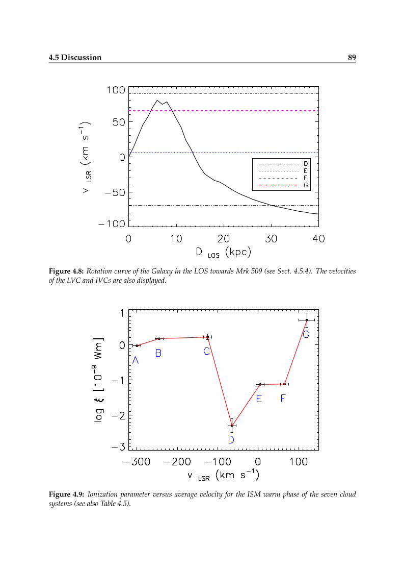
4.5 Discussion 89
Figure 4.8: Rotation curve of the Galaxy in the LOS towards Mrk 509 (see Sect. 4.5.4). The velocitiesof the LVC and IVCs are also displayed.
Figure 4.9: Ionization parameter versus average velocity for the ISM warm phase of the seven cloudsystems (see also Table 4.5).
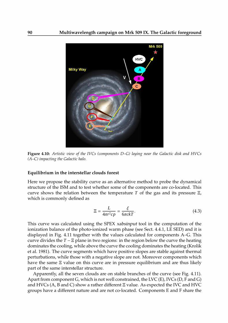
90 Multiwavelength campaign on Mrk 509 IX. The Galactic foreground
Figure 4.10: Artistic view of the IVCs (components D–G) laying near the Galactic disk and HVCs(A–C) impacting the Galactic halo.
Equilibrium in the interstellar clouds forest
Here we propose the stability curve as an alternative method to probe the dynamicalstructure of the ISM and to test whether some of the components are co-located. Thiscurve shows the relation between the temperature T of the gas and its pressure Ξ,which is commonly defined as
Ξ =L
4πr2cp=
ξ
6πckT. (4.3)
This curve was calculated using the SPEX xabsinput tool in the computation of theionization balance of the photo-ionized warm phase (see Sect. 4.4.1, LE SED) and it isdisplayed in Fig. 4.11 together with the values calculated for components A–G. Thiscurve divides the T −Ξ plane in two regions: in the region below the curve the heatingdominates the cooling, while above the curve the cooling dominates the heating (Kroliket al. 1981). The curve segments which have positive slopes are stable against thermalperturbations, while those with a negative slope are not. Moreover components whichhave the same Ξ value on this curve are in pressure equilibrium and are thus likelypart of the same interstellar structure.
Apparently, all the seven clouds are on stable branches of the curve (see Fig. 4.11).Apart from component G, which is not well constrained, the LVC (E), IVCs (D, F and G)and HVCs (A, B and C) show a rather different Ξ value. As expected the IVC and HVCgroups have a different nature and are not co-located. Components E and F share the
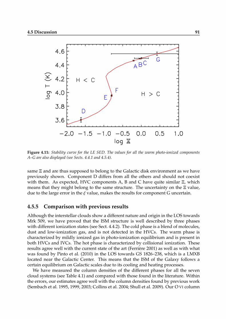
4.5 Discussion 91
Figure 4.11: Stability curve for the LE SED. The values for all the warm photo-ionized componentsA–G are also displayed (see Sects. 4.4.1 and 4.5.4).
same Ξ and are thus supposed to belong to the Galactic disk environment as we havepreviously shown. Component D differs from all the others and should not coexistwith them. As expected, HVC components A, B and C have quite similar Ξ, whichmeans that they might belong to the same structure. The uncertainty on the Ξ value,due to the large error in the ξ value, makes the results for component G uncertain.
4.5.5 Comparison with previous results
Although the interstellar clouds show a different nature and origin in the LOS towardsMrk 509, we have proved that the ISM structure is well described by three phaseswith different ionization states (see Sect. 4.4.2). The cold phase is a blend of molecules,dust and low-ionization gas, and is not detected in the HVCs. The warm phase ischaracterized by mildly ionized gas in photo-ionization equilibrium and is present inboth HVCs and IVCs. The hot phase is characterized by collisional ionization. Theseresults agree well with the current state of the art (Ferriere 2001) as well as with whatwas found by Pinto et al. (2010) in the LOS towards GS 1826–238, which is a LMXBlocated near the Galactic Center. This means that the ISM of the Galaxy follows acertain equilibrium on Galactic scales due to its cooling and heating processes.
We have measured the column densities of the different phases for all the sevencloud systems (see Table 4.1) and compared with those found in the literature. Withinthe errors, our estimates agree well with the column densities found by previous work(Sembach et al. 1995, 1999, 2003; Collins et al. 2004; Shull et al. 2009). Our O VI column

92 Multiwavelength campaign on Mrk 509 IX. The Galactic foreground
densities for the HVCs A–C and the IVC G agree within 1σwith those measured by Foxet al. (2006), who take into account the H2 absorption, which affects this wavelengthrange (see Fig. 4.5). They consider the blend of components A and B as one absorber,but their column density estimate matches the sum of the values that we have obtainedseparately for components A and B. Our total H I column density differs from the valuemeasured at long wavelengths (see Sect. 4.4.1). This is most likely due to the differencebetween the beam-size of the UV and radio observations.
Our determination of the location of the different clouds agrees with previous work,but improves upon the previous results. As discussed in Sect. 4.5.4, the HVCs (A–C)are likely at the outskirts of an extragalactic cloud captured by the Galaxy or the LocalGroup and interacting with them as suggested by Sembach et al. (1999). Component Bhas a |v| lower than component A maybe due to a stronger impact with the Galactic hotgas, as suggested by its higher ionization state. This might indicate that the externallayers of the cloud slewdown during the infall, in agreement with the scenario pro-posed by Lehner & Howk (2011). Such clouds, known also as VHVCs (see Sect. 5.1),are thought to lose their H I and a significant amount of speed during the infall andinteraction with the Galaxy. Moreover, from the similar total pressure and tempera-ture properties measured for the warm phase, we conclude that they likely belong tothe same cloud structure (see Fig. 4.11). Components E (∼ 0km s−1) and F (∼ 60km s−1)have very similar properties for their cold and warm phases and clearly correspond tointerstellar gas which follows the Galactic rotation and are expected to reside at lessthan 1 and 5 kpc, respectively (see Fig. 4.8 and Sect. 4.5.3). This is fully consistent withthe conclusions by Blades & Morton (1983). Component D (∼ −60km s−1) is most likelylocated off the Galactic plane as previously suggested by Morton & Blades (1986), butshould be located at high altitudes.
4.6 Conclusion
We have presented a complete analysis of the interstellar and circumgalactic mediumtowards the AGN Mrk 509, which is a bright X-ray source with a high Galactic latitudeof about −30, through high-quality grating spectra taken with XMM-Newton / RGS,HST / COS and FUSE.
• On average the ISM, as found in the form of LVCs and IVCs near the Galacticdisk, preserves a structure consisting of three distinct main phases with differentionization states. HVCs, which usually probe the halo and CGM, have a differentstructure and in the LOS towards Mrk 509 they show two main phases.
• We have probed seven different cloud systems along the LOS. Our study of theirkinematics and abundances has revealed the nature and location of the cloudswith respect to the Galactic environment assuming Galactic rotation.
• The HVCs (components A–C) are highly ionized most likely as the result of alarger exposure to the X-ray background and the interaction with the circum-galactic medium. The similar abundances and ionization structure suggest a

4.6 Conclusion 93
common origin for these HVCs. They might be at the outskirt of an extragalacticcloud captured by the Galaxy.
• The LVC (component E) and IVC (component F) refer to interstellar gas co-rota-ting with the Galactic disk, as confirmed by the detection of dust and moleculesat rest wavelengths.
• The location of the IVCs (components D and G) is not well constrained, theymight belong either to disk co-rotating gas or to Galactic fountains.
• The column densities, ionization states and locations probed by our alternativemodels/methods agree with each other and with the results in the literature. Allthis supports our research method and justifies extension to more lines-of-sightand/or new observations. These analyses will provide indeed a better mappingof the ISM and a deeper study of its chemical composition and interaction withthe entire Galaxy.
Acknowledgements
This work is based on observations obtained with XMM-Newton, an ESA science mis-sion with instruments and contributions directly funded by ESA Member States andthe USA (NASA). SRON is supported financially by NWO, the Netherlands Organi-zation for Scientific Research. We acknowledge support from NASA/XMM-NewtonGuest Investigator grant NNX09AR01G. Support for HST Program number 12022 wasprovided by NASA through grants from the Space Telescope Science Institute, whichis operated by the Association of Universities for Research in Astronomy, Inc., underNASA contract NAS5-26555. We also acknowledge Rob Detmers for providing us withthe AGN continuum model of Mrk 509. We thank Ken Sembach for helpful discussionson Galactic halo gas and HVCs. We also acknowledge the referee for the useful sug-gestions provided to us, which improve the quality of the paper.

94 Multiwavelength campaign on Mrk 509 IX. The Galactic foreground
Chapter 5
ISM composition through X-rayspectroscopy of LMXBs
C. Pinto1,2, J. S. Kaastra1,3, E. Costantini1, C. de Vries1
1 SRON Netherlands Institute for Space Research, Utrecht, The Netherlands2 Department of Astrophysics, Radboud University, Nijmegen, The Netherlands3 Astronomical Institute, Utrecht University, Utrecht, The Netherlands
Submitted 2 October 2012
Submitted to Astronomy & Astrophysics, 2012
Abstract
The diffuse interstellar medium (ISM) is an integral part of the evolution of the entireGalaxy. Metals are produced by stars and their abundances are the direct testimonyof the history of stellar evolution. However, the interstellar dust composition is notwell known and the total abundances are yet to be accurately determined. We probeISM dust composition, total abundances, and abundance gradients through the studyof interstellar absorption features in the high-resolution X-ray spectra of Galactic low-mass X-ray binaries (LMXBs). We use high-quality grating spectra of nine LMXBstaken with XMM-Newton. We measure the column densities of O, Ne, Mg, and Fewith an empirical model and estimate the Galactic abundance gradients. The columndensities of the neutral gas species are in agreement with those found in the literature.

96 ISM composition through X-ray spectroscopy of LMXBs
We find that solid oxygen is mostly provided by ices and silicates. Respectively, 15–20% and 70–90% of the total amount of O I and Fe I is found in dust. The dust amountand mixture seem to be consistent along all the lines-of-sight (LOS). Our estimates ofabundance gradients and predictions of local interstellar abundances are in agreementwith those measured at longer wavelengths. Our work shows that X-ray spectroscopyis a very powerful method to probe the ISM. For instance, on a large scale the ISMappears to be chemically homogeneous showing similar gas ionization ratios and dustmixtures. The agreement between the abundances of the ISM and the stellar objectssuggests that the local Galaxy is also chemically homogeneous.
5.1 Introduction
The interstellar medium (ISM) is one of the most important component of galaxiesbecause it influences their evolution: the ISM is enriched with heavy elements by stel-lar evolution, and it provides the source of material for following generation of stars.There are several physical processes that alter the metallicity of the ISM. Stellar windsand supernovae expel part of the interstellar gas out of the Galactic disk, but gravitygenerally forces the gas to fall back through the process known as ”Galactic fountain”(Shapiro & Field 1976). Gas accreted from smaller galaxies, like the Magellanic Clouds,and the intergalactic medium increases the reservoir of low metallicity gas. The ISMalso shows a complex structure consisting of phases at different equilibrium temper-atures (for a review, see Draine 2011). The cold phase is a blend of dust, moleculesand almost neutral gas below 104 K. The warm and hot phases are mostly gaseous.The warm gas is weakly ionized, with a temperature of ∼ 104 K. The hot gas is highlyionized, with temperatures of about 106 K. These three main phases are not entirelyseparated from each other. For instance, it is thought that a conductive cooling layer,revealed by O VI, lies between the warm and hot ionized phases (see e.g. Richter 2006).
In the spectra of background sources the ISM produces reddening and absorptionlines. High resolution X-ray spectroscopy has become a powerful diagnostic tool forconstraining the chemical and physical properties of the ISM. The K-shell transitionsof carbon, nitrogen, oxygen, neon, and magnesium, and the L-shell transitions of ironfall in the soft X-ray energy band. The presence of different ionization states constrainsthe multi-phase temperature structure of the ISM. A summary of the results obtainedby X-ray spectroscopy on the ISM in the last decades is given by Pinto et al. (2010).
Briefly, Schattenburg & Canizares (1986) first constrained interstellar oxygen in theX-ray band using the Einstein Observatory, but a thorough study of the ISM was pos-sible only after the launch of the XMM-Newton and Chandra satellites, provided withhigh-resolution gratings. Absorption structure due to ionized gas and dust was foundaround the interstellar oxygen K-shell absorption edge in the spectra of several sources(Paerels et al. 2001; de Vries et al. 2003; Juett et al. 2004; Costantini et al. 2005, 2012; deVries & Costantini 2009; Kaastra et al. 2009; Pinto et al. 2010, 2012a,b).
However, in the last decades, the most important discoveries on the physics of theISM phases have been obtained with UV, IR, optical, and radio spectroscopy. Dust isusually studied in IR, molecules in radio and IR, while the neutral and warm phases

5.1 Introduction 97
of the interstellar gas are also probed with UV data (see Ferriere 2001 and referencestherein). The hot gas is the only ISM phase which is more often studied in X-rays. How-ever, despite the very high resolution and signal-to-noise ratio at long wavelengths,both the chemistry and physics of the interstellar medium are still under debate. Ele-mental abundances, dust depletion factors and dust chemistry are not yet well deter-mined and thus provide an open and interesting research field. The heavy elementssuch as oxygen (the most abundant one) and iron are produced in high-mass stars.Molecules and dust compounds are mainly formed in AGB stars and then grow inthe diffuse ISM (see e.g. Mattsson & Andersen 2012). Heavy elements directly wit-ness the history of the past stellar evolution. In the last years there have been manyattempts to measure the interstellar abundances, but in many cases only lower limitswere obtained due to the depletion of the elements from the gaseous phases into dustgrains and to strong line saturation at long wavelengths. The dust depletion factorsand especially the compounds mixture are not yet well known and thus the total ISMabundances are affected by strong systematic uncertainties. For instance, a significantfraction of the oxygen which is bound in the solid phase is still unknown: silicates andcarbonaceous compounds are not abundant enough to cover the amount of depletedoxygen. Ices may solve this problem, but they are hard to detect (for a review aboutdepletion factors in the ISM see Jenkins 2009). Therefore, our work focuses on an alter-native method to determine ISM column densities, dust depletion factors, molecularcompounds, total abundances (gas + dust), and abundance gradients through X-rayspectroscopy.
In this work we report the detection and modeling of interstellar absorption linesand edges in the high-quality spectra of nine LMXBs: GS 1826−238, GX 9+9, GX 339−4,Aql X−1, SAX J1808.4−3658, Ser X−1, 4U 1254−690, 4U 1636−536, and 4U 1735−444.The observations are taken with the XMM-Newton Reflection Grating Spectrometer(RGS, den Herder et al. 2001), see Table 5.1 for details. These sources are well suitedfor the analysis of the ISM because of their brightness and column densities NH ∼
1 − 5 × 1025 m−2 (see Table 5.2), which are high enough to produce prominent O, Fe,and Ne absorption edges in the soft X-ray energy band. This paper provides a signifi-cant extension of the previous work on the ISM in the line-of-sight (LOS) towards GS1826−238 done by Pinto et al. (2010). We have used updated atomic and moleculardatabase and extended the analysis to several LOS (see Fig. 5.1).
Our analysis focuses on the 7 − 38 Å first order spectra of the RGS detectors. Wehave not used the EPIC spectra of the observations because they have much lowerspectral resolution and we were not interested in determining the source continuumat energies higher than the RGS band. Most of interstellar X-ray features are indeedfound in the soft X-ray energy band. We performed the spectral analysis with SPEX1
version 2.03.03 (Kaastra et al. 1996). We scaled the elemental abundances to the proto-Solar abundances of Lodders & Palme (2009). We use the χ2-statistic throughout thepaper and adopt 1σ errors.
The paper is organized as follows. In Sect. 5.2 we present the data. In Sect. 5.3we report the relevant spectral features that we analyze. In Sect. 5.4 we describe the
1www.sron.nl/spex
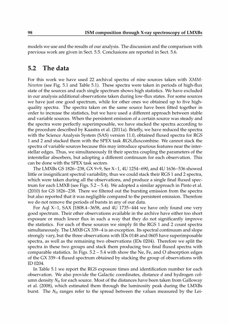
98 ISM composition through X-ray spectroscopy of LMXBs
models we use and the results of our analysis. The discussion and the comparison withprevious work are given in Sect. 5.5. Conclusions are reported in Sect. 5.6.
5.2 The data
For this work we have used 22 archival spectra of nine sources taken with XMM-Newton (see Fig. 5.1 and Table 5.1). These spectra were taken in periods of high-fluxstate of the sources and each single spectrum shows high statistics. We have excludedin our analysis additional observations taken during low-flux states. For some sourceswe have just one good spectrum, while for other ones we obtained up to five high-quality spectra. The spectra taken on the same source have been fitted together inorder to increase the statistics, but we have used a different approach between stableand variable sources. When the persistent emission of a certain source was steady andthe spectra were perfectly superimposable, we have stacked the spectra according tothe procedure described by Kaastra et al. (2011a). Briefly, we have reduced the spectrawith the Science Analysis System (SAS) version 11.0, obtained fluxed spectra for RGS1 and 2 and stacked them with the SPEX task RGS fluxcombine. We cannot stack thespectra of variable sources because this may introduce spurious features near the inter-stellar edges. Thus, we simultaneously fit their spectra coupling the parameters of theinterstellar absorbers, but adopting a different continuum for each observation. Thiscan be done with the SPEX task sectors.
The LMXBs GS 1826−238, GX 9+9, Ser X−1, 4U 1254−690, and 4U 1636−536 showedlittle or insignificant spectral variability, thus we could stack their RGS 1 and 2 spectra,which were taken during all the observations, and produce a single final fluxed spec-trum for each LMXB (see Figs. 5.2 – 5.4). We adopted a similar approach in Pinto et al.(2010) for GS 1826−238. There we filtered out the bursting emission from the spectrabut also reported that it was negligible compared to the persistent emission. Thereforewe do not remove the periods of bursts in any of our data.
For Aql X−1, SAX J1808.4−3658, and 4U 1735−444 we have only found one verygood spectrum. Their other observations available in the archive have either too shortexposure or much lower flux in such a way that they do not significantly improvethe statistics. For each of these sources we simply fit the RGS 1 and 2 count spectrasimultaneously. The LMXB GX 339−4 is an exception. Its spectral continuum and slopestrongly vary, but the three observations with IDs 0148 and 0605 have superimposablespectra, as well as the remaining two observations (IDs 0204). Therefore we split thespectra in these two groups and stack them producing two final fluxed spectra withcomparable statistics. In Figs. 5.2 – 5.4 with show the Ne, Fe, and O absorption edgesof the GX 339−4 fluxed spectrum obtained by stacking the group of observations withID 0204.
In Table 5.1 we report the RGS exposure times and identification number for eachobservation. We also provide the Galactic coordinates, distance d and hydrogen col-umn density NH for each source. Most of the distances have been taken from Gallowayet al. (2008), which estimated them through the luminosity peak during the LMXBsburst. The NH ranges refer to the spread between the values measured by the Lei-
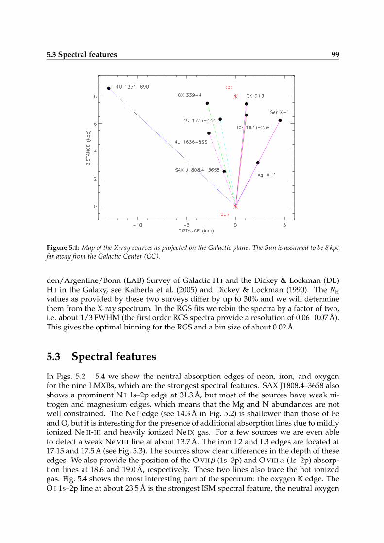
5.3 Spectral features 99
Figure 5.1: Map of the X-ray sources as projected on the Galactic plane. The Sun is assumed to be 8 kpcfar away from the Galactic Center (GC).
den/Argentine/Bonn (LAB) Survey of Galactic H I and the Dickey & Lockman (DL)H I in the Galaxy, see Kalberla et al. (2005) and Dickey & Lockman (1990). The NH
values as provided by these two surveys differ by up to 30% and we will determinethem from the X-ray spectrum. In the RGS fits we rebin the spectra by a factor of two,i.e. about 1/3 FWHM (the first order RGS spectra provide a resolution of 0.06−0.07 Å).This gives the optimal binning for the RGS and a bin size of about 0.02 Å.
5.3 Spectral features
In Figs. 5.2 – 5.4 we show the neutral absorption edges of neon, iron, and oxygenfor the nine LMXBs, which are the strongest spectral features. SAX J1808.4–3658 alsoshows a prominent N I 1s–2p edge at 31.3 Å, but most of the sources have weak ni-trogen and magnesium edges, which means that the Mg and N abundances are notwell constrained. The Ne I edge (see 14.3 Å in Fig. 5.2) is shallower than those of Feand O, but it is interesting for the presence of additional absorption lines due to mildlyionized Ne II-III and heavily ionized Ne IX gas. For a few sources we are even ableto detect a weak Ne VIII line at about 13.7 Å. The iron L2 and L3 edges are located at17.15 and 17.5 Å (see Fig. 5.3). The sources show clear differences in the depth of theseedges. We also provide the position of the O VII β (1s–3p) and O VIII α (1s–2p) absorp-tion lines at 18.6 and 19.0 Å, respectively. These two lines also trace the hot ionizedgas. Fig. 5.4 shows the most interesting part of the spectrum: the oxygen K edge. TheO I 1s–2p line at about 23.5 Å is the strongest ISM spectral feature, the neutral oxygen

100 ISM composition through X-ray spectroscopy of LMXBs
Table 5.1: XMM-Newton/RGS observations used in this paper.
Source ID (a) Length (ks) (b) l, b (c) d (kpc) (d) NH (1025 m−2) (e)
4U 1254–690
0060740901 28.5
303.5,−6.4 15.5 ( f ) 2.2–2.90405510301 60.6
0405510501 60.7
4U 1636–536
0105470401 20.6
332.9,−4.8 5.95 ( f ) 2.6–3.60303250201 30.9
0500350301 31.5
0606070201 28.8
4U 1735–444 0090340201 20.6 346.1,−7.0 6.5 ( f ) 2.6–3.0
Aql X–1 0406700201 52.6 35.7,−4.1 3.9 ( f ) 2.8–3.4
GS 1826–2380150390101 106.3
9.3,−6.1 6.7 ( f ) 1.7–1.90150390301 91.5
GX 339–4
0148220201 20.3
338.9,−4.3 8 (g) 3.7–5.3
0148220301 13.7
0204730201 13.3
0204730301 13.4
0605610201 32.9
GX 9+90090340101 10.6
8.5, 9.0 7.5 (h) 2.0–2.10090340601 21.7
SAX J1808.4–3658 0560180601 63.7 335.4,−8.1 2.77 ( f ) 1.1–1.3
Ser X–1
0084020401 21.5
36.1, 4.8 7.7 ( f ) 4.0–4.70084020501 21.7
0084020601 21.8
(a, b) Identification number and duration of the observation. (c, d, e) Source Galactic coordinates in degrees,
distance from the Sun, and hydrogen column density (see Kalberla et al. 2005 and Dickey & Lockman
1990). ( f ) Distance estimates are taken from Galloway et al. (2008). (g) For GX 339-4 we adopt the
distance as suggested by Zdziarski et al. (2004). (h) The distance for GX 9+9 is the mean value between
those ones provided by Christian & Swank (1997) and Zdziarski et al. (2004).
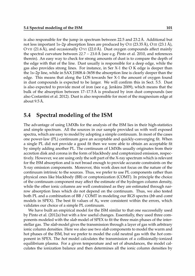
5.4 Spectral modeling of the ISM 101
is also responsible for the jump in spectrum between 22.5 and 23.2 Å. Additional butnot less important 1s–2p absorption lines are produced by O II (23.35 Å), O III (23.1 Å),O VII (21.6 Å), and occasionally O VI (22.0 Å). Dust oxygen compounds affect mainlythe spectral curvature between 22.7 − 23.0 Å (see e.g. Pinto et al. 2010, and referencestherein). An easy way to check for strong amounts of dust is to compare the depth ofthe edge with that of the line. Dust usually is responsible for a deep edge, while thegas also provides strong lines. For instance, in Ser X-1 the O K edge is deeper thanthe 1s–2p line, while in SAX J1808.4–3658 the absorption line is clearly deeper than theedge. This means that along the LOS towards Ser X-1 the amount of oxygen foundin dust compounds is expected to be larger. We will confirm this in Sect. 5.5. Dustis also expected to provide most of iron (see e.g. Jenkins 2009), which means that thebulk of the absorption between 17–17.5 Å is produced by iron dust compounds (seealso Costantini et al. 2012). Dust is also responsible for most of the magnesium edge atabout 9.5 Å.
5.4 Spectral modeling of the ISM
The advantage of using LMXBs for the analysis of the ISM lies in their high-statisticsand simple spectrum. All the sources in our sample provided us with well exposedspectra, which are easy to model by adopting a simple continuum. In most of the casesone power-law (PL) continuum gave an acceptable and quickly-converging fit. Whena single PL did not provide a good fit then we were able to obtain an acceptable fitby simply adding another PL. The continuum of LMXBs usually originates from theiraccretion disk and corona in the form of blackbody and comptonized emission, respec-tively. However, we are using only the soft part of the X-ray spectrum which is relevantfor the ISM absorption and is not broad enough to provide accurate constraints on theX-ray emission components. Moreover, this work does not focus on the nature of thecontinuum intrinsic to the sources. Thus, we prefer to use PL components rather thanphysical ones like blackbody (BB) or comptonization (COMT). In principle the choiceof the continuum component may affect the estimate of the hydrogen column density,while the other ionic columns are well constrained as they are estimated through nar-row absorption lines which do not depend on the continuum. Thus, we also testedboth PL and a combination of BB / COMT in modeling our RGS spectra (bb and comtmodels in SPEX). The best fit values of NH were consistent within the errors, whichvalidates our choice of a simple PL continuum.
We have built an empirical model for the ISM similar to that one successfully usedby Pinto et al. (2012a) but with a few useful changes. Essentially, they used three com-ponents modeled with the slab model of SPEX to fit the three main phases of the inter-stellar gas. The slab model gives the transmission through a layer of gas with arbitraryionic column densities. Here we also use two slab components to model the warm andhot phases of the ISM, but we prefer to model the cold neutral gas with the hot com-ponent in SPEX. The hot model calculates the transmission of a collisionally-ionizedequilibrium plasma. For a given temperature and set of abundances, the model cal-culates the ionization balance and then determines all the ionic column densities by

102 ISM composition through X-ray spectroscopy of LMXBs
4050
60
NeIX
NeINeIII
NeII
4U 1254−690
9010
011
012
0
Flu
x (p
hoto
ns m
−2
s−1
A−
1 )
GS 1826−238
13.5 14 14.5 15100
120
140
160
Wavelength (Å)
Ser X−1
100
120
140
NeIX
NeINeIII
NeII
4U 1636−536
250
300
350
GX 9+9
13.5 14 14.5 154050
6070
Wavelength (Å)
GX 339−4
200
250
300
NeIX
NeI
NeIII
NeII
4U 1735−444
150
200
250
Aql X−1
13.5 14 14.5 15200
220
240
260
Wavelength (Å)
SAX J1808.4−3658
Figure 5.2: Data and best-fitting models: the Ne K edge.
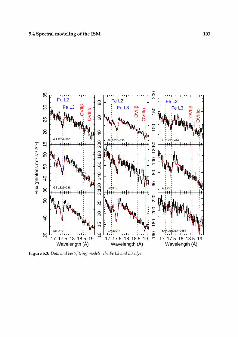
5.4 Spectral modeling of the ISM 103
1520
2530
35
Fe L2
Fe L3
OV
IIβO
VIII
α
4U 1254−690
3040
5060
Flu
x (p
hoto
ns m
−2
s−1
A−
1 )
GS 1826−238
17 17.5 18 18.5 192040
60
Wavelength (Å)
Ser X−1
4060
80Fe L2
Fe L3
OV
IIβO
VIII
α4U 1636−536
120
140
160
180
200
GX 9+9
17 17.5 18 18.5 191015
2025
30
Wavelength (Å)
GX 339−4
5010
015
020
0
Fe L2Fe L3
OV
IIβO
VIII
α
4U 1735−444
6080
100
120
Aql X−1
17 17.5 18 18.5 19160
180
200
220
Wavelength (Å)
SAX J1808.4−3658
Figure 5.3: Data and best-fitting models: the Fe L2 and L3 edge.
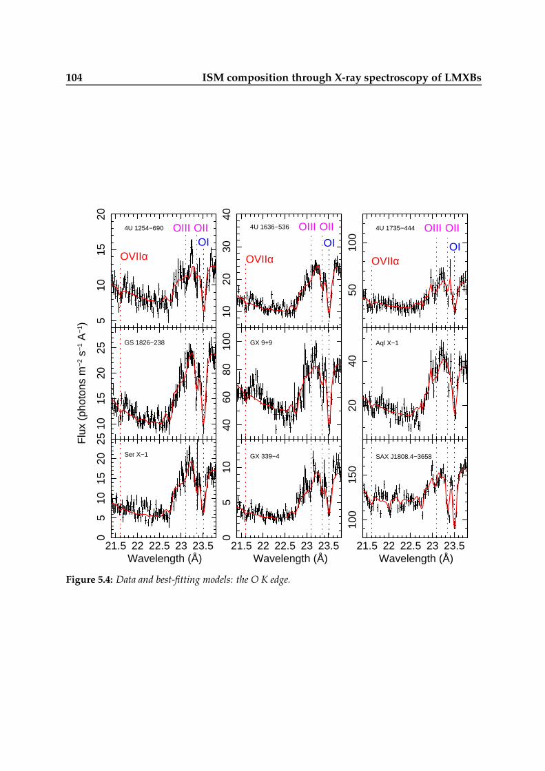
104 ISM composition through X-ray spectroscopy of LMXBs
510
1520
OVIIα
OIII OIIOI
4U 1254−690
1015
2025
Flu
x (p
hoto
ns m
−2
s−1
A−
1 )
GS 1826−238
21.5 22 22.5 23 23.5
05
1015
2025
Wavelength (Å)
Ser X−1
1020
3040
OVIIα
OIII OII
OI
4U 1636−53640
6080
100
GX 9+9
21.5 22 22.5 23 23.5
05
10
Wavelength (Å)
GX 339−4
5010
0
OVIIα
OIII OII
OI
4U 1735−444
2040
Aql X−1
21.5 22 22.5 23 23.5
100
150
Wavelength (Å)
SAX J1808.4−3658
Figure 5.4: Data and best-fitting models: the O K edge.

5.4 Spectral modeling of the ISM 105
scaling to the prescribed total hydrogen column density. At low temperatures thismodel mimics very well the neutral interstellar gas (see SPEX manual and Kaastraet al. 2009). Free parameters in the hot model are the hydrogen column density NH,the temperature T , the velocity dispersion σv, the systematic velocity v, and the abun-dances. However, in X-rays the spectral resolution is not high enough to constrain thevelocities with sufficient accuracy, thus we assume that the interstellar gas is at rest.We also assume a temperature of 0.5 eV (about 5800 K), the lowest value available inthe SPEX hot model, because in this way the gas is mostly neutral. In X-rays withthe current satellites it is not possible to resolve the narrow lines of the interstellarmedium. A spectral fit can easily provide a wrong value of velocity dispersion σv andconsequently of column density because they are degenerate. Therefore it is more ap-propriate adopting a physically reasonable value for the σv and just fitting the columndensity of each ion. We adopt a nominal value of 10 km s−1 for the velocity dispersionof the cold (O I) and warm (O II-V) gas components, which is similar to that foundby Pinto et al. (2012a) using a higher-resolution UV spectrum. For the hot gas (O VI
and higher ionization states) we adopt σv =100 km s−1, which is an average value be-tween those suggested in the literature (see for instance the work by Yao & Wang 2005and Yao et al. 2009a on high-resolution Chandra X-ray spectra of several LMXBs). Wetook into account absorption by interstellar dust with the SPEX amol component. Theamol model calculates the transmission of various molecules, for details see Pinto et al.(2010), Costantini et al. (2012) and the SPEX manual. The model currently takes intoaccount the modified edge and line structure around the O and Si K-edge, and the FeK / L-edges, using measured cross sections of various compounds taken from the lit-erature. Relevant and abundant silicates, ices and organic molecules are present in theour database. In fitting the molecular models we limit the range of column densitiesto physical values. For instance, we took care that the column density of each weakly-abundant element did not exceed the proto-Solar value predicted by the best-fittingNH. This is important especially for Ca and Al (contained respectively in andraditeand hercinite), whose abundances are much lower than oxygen.
5.4.1 Results
The results of our best fitting model obtained on the X-ray sources are shown in Ta-ble 5.2 and plotted in Figs. 5.2–5.4. The model fits very well both the absorption edgesand lines. We show the absolute abundances and hydrogen column density for thecold gas, the column densities for all ions and molecules that we were able to detect.In the cases of no detection we report the 2σ upper limits. We also report the formulafor each compound and the total amount of iron and oxygen found in dust. We willdiscuss the results in Sect. 5.5. Briefly, we have found a general agreement in the spec-tra of the different sources. Ions like O V-VI and molecular compounds like hematite(Fe2O3), and CO are hard to detect. Instead, O VII-VIII, H2O ices, and compounds ofCa (andradite), and Al (Hercinite) are detected along any LOS. The cold neutral gasprovides on average O I ∼ 1− 3× 10²² m−2, which means that most oxygen is found inthe neutral phase. We have summed all the contributions to the molecular oxygen aswell as all the ionic column densities of the mildly ionized (O II-V) and heavily ionized
106 ISM composition through X-ray spectroscopy of LMXBs
(O VI-VIII) gas, and compare them in Table 5.3. As we have mentioned above, mostof the oxygen is provided by the neutral gas phase. Dust also seems to be ubiquitous.The warm and hot ionized gas phases generally contribute less to oxygen, but there aresome cases in which they constitute significant portions of the total column density.
5.4.2 Limitations
There are some factors that may limit and affect the uniqueness of our best-fitting mod-els. First of all, the features produced by molecules in a certain absorption edge aresimilar and degenerate. Near the Fe L-edge the RGS absorption lines blend and maynot give unique solutions. Chandra spectra are provided with higher resolution, butthey give accurate results only for a few sources even brighter than ours. Therefore,in our standard modeling we have simultaneously fitted all the molecules and all theabsorption edges and lines in order to obtain the best-fitting mixture and to break asmuch as possible the degeneracy. Unfortunately, for some compounds, such as mag-netite and pyroxene, we only have the transmission near the oxygen edge, while forthe other edges we simply use the pure atomic cross-section without absorption lines(for details consult the amol model in the SPEX manual). As we already mentioned,we performed additional fits with different combinations of molecules by excludingsome of them. However, the total amount of oxygen and iron in dust did not stronglydepend on the chosen dust mixture. Therefore, their depletion factors are not highlyeffected, while the detailed chemical structure may be.
On another hand, the molecular database is not complete. We have tested all themolecules available in the SPEX database, which are about 40 (carbon oxides, ices, ironand magnesium silicates, and more complex molecules). Although these compoundsare among the most abundant in the ISM, we could still miss important contributionfrom other species like forsterite (Mg2 Si O4, see e.g. Jones 2000). For instance, we mayhave overestimated the presence of water ice, as in the diffuse interstellar mediumits amount should be small (Jenkins 2009). As mentioned in Sect. 5.4 concerning thespectral fitting, we have limited the column densities of the molecules responsible forAl (hercinite) and Ca (andradite). If the O/Ca and O/Al ratios in the ISM moleculesare higher than those of our sample, then the amount of oxygen in silicates and otheroxides can increase at the expense of ices. Moreover, there is some degeneracy due tothe similarity of the absorption profiles of ice and pyroxene (see e.g. Costantini et al.2012), which would require spectra with higher signal-to-noise ratios.
The results obtained on the various absorption edges have different weights. Theoxygen edge is the deepest and the column densities of oxygen compounds are con-strained better than for iron. The Mg edge is very weak for hydrogen column densitieslike those of our sources and the estimates of magnesium abundances and depletionfactors are much more uncertain. This does not apply to neon as it is supposed to beonly in a gaseous phase. This work mostly focuses on measurements of interstellaroxygen, iron, and neon column densities. A deep analysis of magnesium and siliconwould require the use of both the XMM-Newton RGS and the Chandra HETG gratings(which have higher effective area and resolution than RGS at short wavelength) incombination with sources with higher hydrogen column densities.
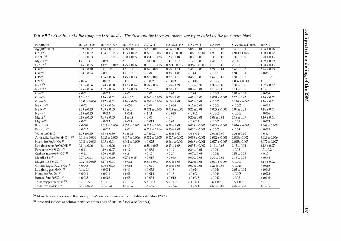
5.4
Sp
ectra
lm
od
elin
go
fth
eIS
M1
07
Table 5.2: RGS fits with the complete ISM model. The dust and the three gas phases are represented by the four main blocks.
Parameter 4U1254–690 4U 1636–536 4U 1735–444 Aql X–1 GS 1826–238 GX 339–4 GX 9+9 SAX J1808.4–3658 Ser X-1
NH (1025 m−2) 2.69 ± 0.02 3.58 ± 0.07 3.28 ± 0.01 5.21 ± 0.03 4.14± 0.06 5.08 ± 0.01 2.15 ± 0.05 1.40 ± 0.01 4.98 ± 0.16
O/H (a) 0.92 ± 0.02 0.840± 0.013 0.93 ± 0.02 0.878 ± 0.007 0.915± 0.009 1.061 ± 0.004 0.99 ± 0.02 0.913± 0.025 0.90 ± 0.02
Ne/H (a) 0.91 ± 0.03 1.315± 0.015 1.00 ± 0.05 0.951 ± 0.025 1.23± 0.04 1.05 ± 0.05 1.35 ± 0.07 1.37± 0.05 1.20± 0.05Mg/H (a) 1.7 ± 0.3 < 0.20 2.0 ± 0.3 1.00 ± 0.13 1.41± 0.12 1.17 ± 0.05 0.41 ± 0.25 < 0.16 0.89 ± 0.09
Fe/H (a) 0.16 ± 0.05 0.176 ± 0.017 0.25 ± 0.06 0.113 ± 0.015 0.224± 0.017 0.365 ± 0.006 0.19 ± 0.03 < 0.02 0.50± 0.03O II (b) 0.33 ± 0.10 1.4 ± 0.2 0.6 ± 0.2 0.04 ± 0.02 0.60 ± 0.11 1.41 ± 0.06 0.27 ± 0.04 1.67 ± 0.03 2.24 ± 0.13
O III (b) 0.08 ± 0.04 < 0.1 0.2 ± 0.1 < 0.04 0.08 ± 0.05 < 0.04 < 0.05 0.34 ± 0.01 < 0.03
O IV (b) 0.5 ± 0.1 0.86 ± 0.06 0.45 ± 0.13 0.37 ± 0.07 0.79 ± 0.13 0.48 ± 0.03 0.62 ± 0.07 0.31 ± 0.03 1.5 ± 0.2
O V (b) < 0.04 < 0.013 < 0.1 < 0.032 < 0.063 < 0.013 < 0.002 0.006 ± 0.001 0.3 ± 0.1
Ne II (b) 0.11 ± 0.06 1.70 ± 0.08 0.47 ± 0.14 0.66 ± 0.14 1.58 ± 0.24 1.17 ± 0.32 0.32 ± 0.06 1.32 ± 0.06 0.32 ± 0.07
Ne III (b) 0.25 ± 0.06 0.82 ± 0.06 0.52 ± 0.13 1.2 ± 0.2 0.79 ± 0.15 0.85 ± 0.04 0.18 ± 0.05 1.14 ± 0.08 0.8 ± 0.1
O VI (b) < 0.01 < 0.025 < 0.01 < 0.05 < 0.02 < 0.01 < 0.003 0.02 ± 0.01 < 0.016
O VII (b) 2.3 ± 0.1 0.16 ± 0.01 4.4 ± 0.3 0.046 ± 0.003 0.23 ± 0.06 4.42 ± 0.06 0.038 ± 0.002 2.25 ± 0.42 0.20 ± 0.02
O VIII (b) 0.082 ± 0.006 0.17 ± 0.01 0.24 ± 0.09 0.089 ± 0.004 0.10 ± 0.01 0.42 ± 0.01 < 0.005 0.110 ± 0.005 0.24 ± 0.01
Ne VIII (b) < 0.02 0.08 ± 0.04 < 0.056 < 0.09 < 0.004 0.12 ± 0.04 < 0.004 < 0.003 < 0.003
Ne IX (b) 2.48 ± 0.13 0.09 ± 0.03 3.5 ± 0.4 0.071 ± 0.003 0.028 ± 0.003 0.21 ± 0.01 0.025 ± 0.003 0.05 ± 0.02 0.14 ± 0.01
Ne X (b) 0.15 ± 0.13 < 0.003 < 0.074 < 1.11 < 0.025 < 0.002 < 0.006 < 0.008 < 0.006
Mg XI (b) 0.16 ± 0.03 0.08 ± 0.03 1.1 ± 0.9 < 0.05 < 0.1 0.20 ± 0.04 0.08 ± 0.02 0.18 ± 0.09 0.10 ± 0.04
Mg XII (b) < 0.01 < 0.002 < 0.008 < 0.013 < 0.02 < 0.0013 < 0.005 < 0.01 < 0.003
Fe XVII (b) < 0.001 0.023 ± 0.006 0.025 ± 0.012 0.017 ± 0.004 0.03 ± 0.01 0.016 ± 0.002 0.008 ± 0.004 0.026 ± 0.005 0.006 ± 0.003
Fe XVIII (b) < 0.017 < 0.013 < 0.011 0.029 ± 0.014 0.03 ± 0.02 0.012 ± 0.007 < 0.003 < 0.04 < 0.003
Water ice H2 O (b) 2.05 ± 0.35 0.88 ± 0.30 3.4 ± 0.6 2.7 ± 0.2 2.63 ± 0.45 4.4 ± 0.2 2.01 ± 0.05 0.34 ± 0.10 < 0.42Andradite Ca3 Fe2 Si3 O12
(b) 0.016 ± 0.004 0.023 ± 0.003 0.017 ± 0.006 0.032 ± 0.005 0.027 ± 0.002 0.033 ± 0.002 0.012 ± 0.004 0.008± 0.002 0.029 ± 0.006
Hercinite Fe Al2 O4(b) 0.041 ± 0.003 0.05 ± 0.01 0.041 ± 0.009 < 0.025 0.061 ± 0.004 0.069 ± 0.001 0.027 ± 0.007 0.015± 0.007 0.072 ± 0.007
Lepidocrocite Fe O (OH) (b) 0.11 ± 0.06 0.41 ± 0.06 < 0.13 0.58 ± 0.05 0.43 ± 0.08 0.035 ± 0.002 0.19 ± 0.03 0.15 ± 0.04 0.15 ± 0.07
Pyroxene Mg Si O3(b) < 0.11 1.19 ± 0.07 < 0.12 < 0.088 < 0.19 0.34 ± 0.01 < 0.014 < 0.03 1.7 ± 0.2
Carbon monoxide CO (b) < 0.11 0.29 ± 0.15 < 0.2 < 0.12 < 0.29 0.07 ± 0.05 < 0.046 0.58 ± 0.03 < 0.17
Metallic Fe (b) 0.27 ± 0.01 0.25 ± 0.10 0.27 ± 0.15 < 0.017 < 0.033 0.60 ± 0.01 0.33 ± 0.02 0.13 ± 0.01 < 0.044
Magnetite Fe3 O4(b) 0.027 ± 0.015 0.17 ± 0.01 < 0.032 0.34 ± 0.01 0.31 ± 0.03 0.20 ± 0.01 0.011 ± 0.007 < 0.005 0.18 ± 0.02
Olivine Mg1.6 Fe0.4 SiO4(b) < 0.043 0.06 ± 0.03 < 0.084 < 0.041 0.05 ± 0.03 0.07 ± 0.01 0.21 ± 0.05 < 0.026 < 0.085
Laughing gas N2O (b) 0.4 ± 0.1 < 0.034 < 0.11 < 0.033 < 0.18 < 0.024 < 0.026 0.03 ± 0.02 < 0.043
Hematite Fe2 O3(b) < 0.041 < 0.011 < 0.08 < 0.014 < 0.16 < 0.003 < 0.016 < 0.008 < 0.022
Iron sulfate Fe SO4(b) < 0.035 < 0.006 < 0.05 < 0.034 < 0.012 < 0.0035 < 0.042 < 0.03 < 0.016
Total oxygen in dust (b) 3.2 ± 0.5 7 ± 1 4.2 ± 0.7 5.7 ± 0.6 5.6 ± 0.8 7.3 ± 0.4 3.6 ± 0.5 1.5 ± 0.2 7 ± 1
Total iron in dust (b) 0.54 ± 0.07 1.3 ± 0.2 0.5 ± 0.2 1.7 ± 0.1 1.5 ± 0.2 1.4 ± 0.1 0.65 ± 0.05 0.32 ± 0.03 0.8 ± 0.1
(a) Abundances ratios are in the linear proto-Solar abundance units of Lodders & Palme (2009).
(b) Ionic and molecular column densities are in units of 1021 m−2 (see also Sect. 5.4).
108 ISM composition through X-ray spectroscopy of LMXBs
Our estimates of column densities and abundances provide interstellar propertiesas integrated along the LOS and on a large scale. This is reasonable for the diffusegas, which is almost uniformly distributed between 3–15 kpc from the Galactic Centerand whose warm phase may reach a few kpc height from the Galactic place (see e.g.Ferriere 2001). This scale-height is indeed comparable to the average altitude of oursources (see Table 5.1). However, this assumption may not be correct for dust andmolecules, which follow the Galactic spirals and are usually found at lower altitudes.This means that dust sampling towards our targets may be closer to the Sun ratherthan in the middle of the path. In the cold phase, iron and magnesium are stronglydepleted into dust. Therefore, the average location of the Fe and Mg absorbers canbe found at shorter distances than those referring to oxygen and neon. However, inSect. 5.5.2 we will show that along our low-latitude LOS the different scale-heights ofgas and dust will not affect the results.
5.5 Discussion
Our analysis shows that the ISM has a multi-phase structure characterized by cold neu-tral gas (and dust), mildly ionized gas and heavily ionized gas. This complex structureis found towards any of the studied sources (see Table 5.2) and is consistent with ourprevious work (see e.g. Kaastra et al. 2009; Pinto et al. 2010, 2012a; Costantini et al.2012). Signatures of dust are always present with main contributions by ices and sili-cates. The oxygen edge and lines provide the most accurate results due to their largedepth, but the results are even more robust because of the simultaneous modeling of allthe absorption edges. This was crucial especially for fitting dust and molecules whichaffect both O, Fe, and Mg edges. An interesting and simple check of different amountsof oxygen in dust is provided by the comparison of the O K edge in Fig. 5.4. As we an-ticipated in Sect. 5.3, the O I 1s–2p absorption line is deeper than the oxygen edge forSAX J1808.4−3658, while for Ser X–1 and GX 339–4 they are comparable. We attributethis to oxygen depleted from the gas phase into dust grains, which is confirmed by themeasurement of a larger amount of oxygen in solids in the LOS towards the two lattersources (see Table 5.2).
5.5.1 The nature of the gas phases
In our standard model we have used a collisionally-ionized model in SPEX because atlow temperatures this mimics well the cold interstellar gas. However, at these temper-atures photo-ionization could also provide a significant contribution. Therefore, wetried an alternative model in which a photo-ionized component (xabs in SPEX) substi-tutes the cold collisionally-ionized hot component. The fits are equivalent, the gas isalmost neutral with a very low ionization parameter ξ. Abundances and χ2 are consis-tent with our standard model. The main difference is that the fit with the photo-ionizedmodel takes more time to converge and the absolute abundances, i.e. relative to hy-drogen, have larger uncertainties (see also Pinto et al. 2012a). Therefore, we prefer tokeep our standard model even if photo-ionization is not ruled out.
5.5 Discussion 109
We have also considered an alternative, physical model for the warm mildly-ionizedgas that produces most of the O II-IV and Ne II-III absorption lines. Instead of a slababsorber we have tested a photo-ionized xabs component, which was successfully usedby Pinto et al. (2012a) in the deep UV and X-ray spectra of the AGN Mrk 509. The fitwas bad because a single photo-ionized component is not able to fit all the large columndensities as measured by our empirical standard model and shown in Table 5.2. Weneed a low-ionization component which provides the bulk of O II and Ne II togetherwith an intermediate-ionization component for the other ions. Interestingly, a good fitis obtained when using the same abundance pattern as provided by the cold neutralgas, while proto-Solar abundances give a bad fit. However, a thorough study of thewarm gas requires longer exposures and complementary UV data, which is beyondthe scope of this paper.
The heavily ionized gas is usually found to be in collisional equilibrium. However,it is thought that this hot gas in the Galaxy is not characterized by a single phase,but it is constituted of two main phases. Most O VII-VIII should arise from a very hot(∼ 2 × 10⁶ K) collisionally-ionized phase, while the bulk of O VI is thought to be em-bedded in a cooling phase with temperatures 1− 5 × 10⁵ K (see e.g. Richter 2006). Wehave tested both single-phase and two-phase models by substituting the slab compo-nent responsible for the O VI-VIII absorption with one and two collisionally-ionizedhot components in SPEX. The fits are comparable due to the weakness of their absorp-tion lines. We would need UV O VI data in order to put strong constraints, but mostof our targets have not been observed with COS/HST or FUSE. However, Table 5.2shows a spread larger than 10 in the O VII / O VIII column ratio, which for a single gascomponent would provide a very large scatter in temperature between the nine LOS(from 1.2 to 2.6 million K). We think that combinations of two stable, but different hot(cooling and coronal) phases is a more likely description.
5.5.2 Is the ISM chemically homogeneous ?
On small scales the ISM is not expected to be highly homogeneous because there aresignificant physical and chemical differences between the interstellar environmentslike H II regions, PNe nebulae, dark clouds, etc. However, the diffuse medium in ourGalaxy may be homogeneous on large scales. Some chemical and physical proper-ties may be possibly consistent when comparing distant regions which underwent asimilar evolution. This is possible for dust as most of it is expected to grow in the ISMrather than in stars (see e.g. Mattsson & Andersen 2012). It is thus worth to compare itschemical properties as integrated along the different LOS. First of all, we notice that themolecular composition is similar in any direction. Aluminates and calcium silicates arefound to provide most of Al and Ca, which are indeed expected to be highly depletedinto dust. Even more interesting is the detection of water ice which was suggested byJenkins (2009) as a possible principal resource of oxygen in dust and a solution to theproblem of oxygen depletion. The same applies to metallic iron. We remark that theamount of water ice as measured by us may be overestimated due to the small sam-ple of molecules in the current database (see Sect. 5.4.2). Cross-sections of additionalcompounds are currently being measured and may provide more accurate results. To

110 ISM composition through X-ray spectroscopy of LMXBs
understand the role of dust, we have summed all the contributions to oxygen fromsolids and molecules and compared it with the hydrogen column density that we haveobtained in our best fits (see Fig. 5.5). We show the trends of both the total column den-sity of dusty oxygen and its fraction with respect to the total amount of neutral oxygen(gas + dust) as function of the NH. The oxygen dust column correlates well with thehydrogen column density (slope = (1.4± 0.1)× 10−4) and the fraction of oxygen boundin dust is constant (18± 3%) along any LOS. These results suggest that on average thecold ISM phase is chemically homogeneous. We notice that the total amount of oxygenin dust is solidly measured as it does not strongly depend on the dust mixture. Forinstance, we tested different molecular combinations by removing some of the maincompounds from the fit, but in the end the sum of all the oxygen molecular columndensities provide the same results in the fits. The same applies for iron, whose dustfraction does not depend on the NH and the LOS, but it has a larger uncertainty andspreads between 70–90%. This occurs because the iron L edge is shallower than theoxygen K edge. As we mentioned in Sect. 5.4.2, the scale-height of the interstellar dustis smaller than for the gas, thus, due to the altitudes of the targets, the dust is expectedat shorter distances from the Sun. This means that the analysis of the dust in thesedifferent LOS probes properties of the ISM as measured on a large scale, but proba-bly smaller than with the gas. As additional check we have computed the dust-to-gasratio for our sources as the ratio between the total amount of oxygen in dust and thehydrogen column density. The dust-to-gas ratio is constant (slope = −0.027± 0.034) atany value of Galactic latitude as shown in Fig. 5.6. This result and the trend seen inFig. 5.5 suggest that the distribution of the dust should not deviate from the gas. Thismay be due to the low latitudes of our sources, which was also one of the reasons forus to choose these targets as representatives of the Galactic (inner) disk.
5.5.3 ISM column densities
Our empirical model provides us with estimates of column densities for several molec-ular and ionic species (see Table 5.2). In some cases we could only obtain upper limits,but we prefer to show them as they may be useful for future work. In order to furthercheck the robustness of our model we compare our column density estimates withthose found in the literature. In most cases our best-fit values of NH agree with thosemeasured at longer wavelength (see Table 5.1). On average our values are slightlyhigher that the 21 cm H I estimates probably because the curvature as measured in theX-ray above 25 Å takes into account the contributions from H I and H2. Our valuesare consistent with other papers (see e.g. Xiang et al. 2005; Caballero-Garcıa et al. 2009;Bhattacharyya & Strohmayer 2007; Patruno et al. 2009). Our column density estimatefor GS 1826–238 agrees with what we found with a different model in Pinto et al. (2010),i.e. NH = 4.14±0.07×1025 m−2. All the neutral column densities that we have measuredfor 4U 1636–536, 4U 1735-444, GX 339–4, GX 9+9, and Ser X-1 are consistent with Juettet al. (2004, 2006). We found a disagreement between our average values of O II/O I
and O III/O I column density ratios, ∼0.06 and ∼0.01 respectively, with those obtainedby Juett et al. (2004) of about 0.1. This may be due to the fact that their model does nottake into account any contribution by dust or molecules near 23 Å and thus may over-

5.5 Discussion 111
Figure 5.5: Amount of O I in dust and its fraction with respect to the total neutral oxygen (gas + dust)versus the hydrogen column density.
Figure 5.6: Ratio between the Amount of O I in dust and the hydrogen column density versus theabsolute value of the Galactic latitude.

112 ISM composition through X-ray spectroscopy of LMXBs
estimate the amount of ionized oxygen. Our O VII column densities are significantlylarger than those estimated by Miller et al. (2004) for GX 339–4 probably because theyhave adopted a much larger velocity dispersion or because of saturation which usu-ally affects absorption lines with σ > 60km s−1 (see e.g. Yao & Wang 2005). We pointout that many of the high-resolution X-ray (RGS) spectra of these sources have beenanalyzed for the first time by us.
5.5.4 ISM abundances
We have also estimated the total abundances of O, Ne, Mg, and Fe for the cold phasein units of Lodders & Palme (2009) by summing, for each element, the contributionsfrom neutral gas, dust, and molecules (see Table 5.4). In most cases all the elementsappear to be over-abundant with respect to the proto-Solar values. This is expected asall LOS cross inner Galactic regions where the abundances are higher. It is very diffi-cult to estimate the location of the absorbing medium for several reasons. At first, weintegrate over the LOS and thus our abundances have to be considered as large-scaleproperties of the ISM. Moreover, the ISM mass-density distribution within the Galaxyis not well known and the LMXB distances are affected by a large uncertainty whichwill dominate the error on the ISM absorber location. Therefore, we adopt half of thedistance to each LMXB as a first-order, average-distance indicator. This means thatthe Galactocentric radius RG of each ISM absorber will be defined as the distance fromthe Galactic Center (hereafter GC) to the mean point of the segment which connectsthe Sun to each target. We show the abundance trends for O, Ne, Mg, and Fe withrespect to RG (in kpc) in Fig. 5.7. These trends were fitted with a linear function and weobtained the following abundance gradients:
12+ log (O/H) = (8.98± 0.03)− (0.023± 0.006)× RG ,
12+ log (Fe/H) = (7.75± 0.13)− (0.033± 0.023)× RG ,
12+ log (Ne/H) = (8.33± 0.03)− (0.031± 0.006)× RG ,
12+ log (Mg/H) = (7.87± 0.10)− (0.028± 0.020)× RG .
The plots show that only the oxygen abundance is clearly anti-correlated with the dis-tance from the GC. Neon also shows a gradient but with a large scatter probably dueto contribution intrinsic to the sources (see e.g. Juett & Chakrabarty 2003 and Madejet al. 2010). However, the linear fits show negative gradients for all the abundanceswhich is consistent with the fact that stellar evolution proceeds faster in the Galacticinner regions. Interestingly, our abundance gradients agree with those estimated withdifferent methods and in different wavelength regimes (Maciel & Quireza 1999; Rolle-ston et al. 2000; Esteban et al. 2005; Pedicelli et al. 2009). On average our values areslightly smaller than those found in the literature. An explanation may be that weoverestimated the distance of the absorbers by a (small) systematic factor. In fact, theLMXBs are not exactly in the Galactic Plane, but are above or below by some hundredsparsec. This means that the distance of each ISM absorber, as projected on the Galacticplane, should be smaller than what we have adopted. The altitudes of the LMXBs alsoaffect the abundance estimates because of the (negative) vertical metallicity gradient

5.5 Discussion 113
(see e.g. Pedicelli et al. 2009). The slopes of the radial and vertical gradients are similar(we have compared their effects in Pinto et al. 2012a). The sources have low latitudes(see Table5.1), on average we obtained b ∼ 6.1, which implies that the radial abun-dance variations are about 10 times larger than the vertical ones. This explains whyignoring the vertical gradient may only marginally affect our results. We may haveunderestimated the Mg and Fe abundance gradients also because in the cold phasethese elements are locked up into dust. In fact, as reported in Sect. 5.4.2, dust could befound at distances shorter than the gas along our LOS. This means that the average dis-tances of the Fe and Mg absorbers may be smaller and the gradients higher than thoseestimated. However, once taken all this into account, our estimates of abundance gra-dients agree even better with the literature.
We can also predict the local proto-Solar interstellar abundances and check if theyagree with those found in the Solar system. According to the equation above, we cal-culate that at the Galactocentric radius of the Sun, which is ∼8.0 kpc (see e.g. Malkin2012), the predicted proto-Solar abundances are
12+ log (O/H)⊙ = (8.80± 0.05),
12+ log (Fe/H)⊙ = (7.48± 0.23),
12+ log (Ne/H)⊙ = (8.08± 0.05),
12+ log (Mg/H)⊙ = (7.66± 0.19).
These values agree very well with the abundances in the Solar System as measuredby Lodders & Palme (2009) [O/H]= 8.76, [Fe/H]= 7.54, [Ne/H]= 7.95, [Mg/H]= 7.62,and further validate our method. Interestingly, the interstellar oxygen abundance, asmeasured by previous work, is always lower than the abundance estimates for theSolar System, OB stars, H II regions, planetary nebulae, Cepheids, and Sun-like stars(see e.g. Stasinska et al. 2012 and Nieva & Przybilla 2012). Instead, our measurementsand predictions agree very well with the abundances of these stellar indicators, whichconfirms that the local Galaxy is chemically homogeneous (see also Stasinska et al.2012).
As clearly seen in Fig. 5.7, our work is optimal to probe ISM abundances within4–8 kpc from the GC, but this range could be easily extended by using more sources.This may be an interesting proxy for a future work extended to more LOS and back-ground source types like LMXBs, novae and AGN (especially Blazars, which do notshow significant intrinsic features).
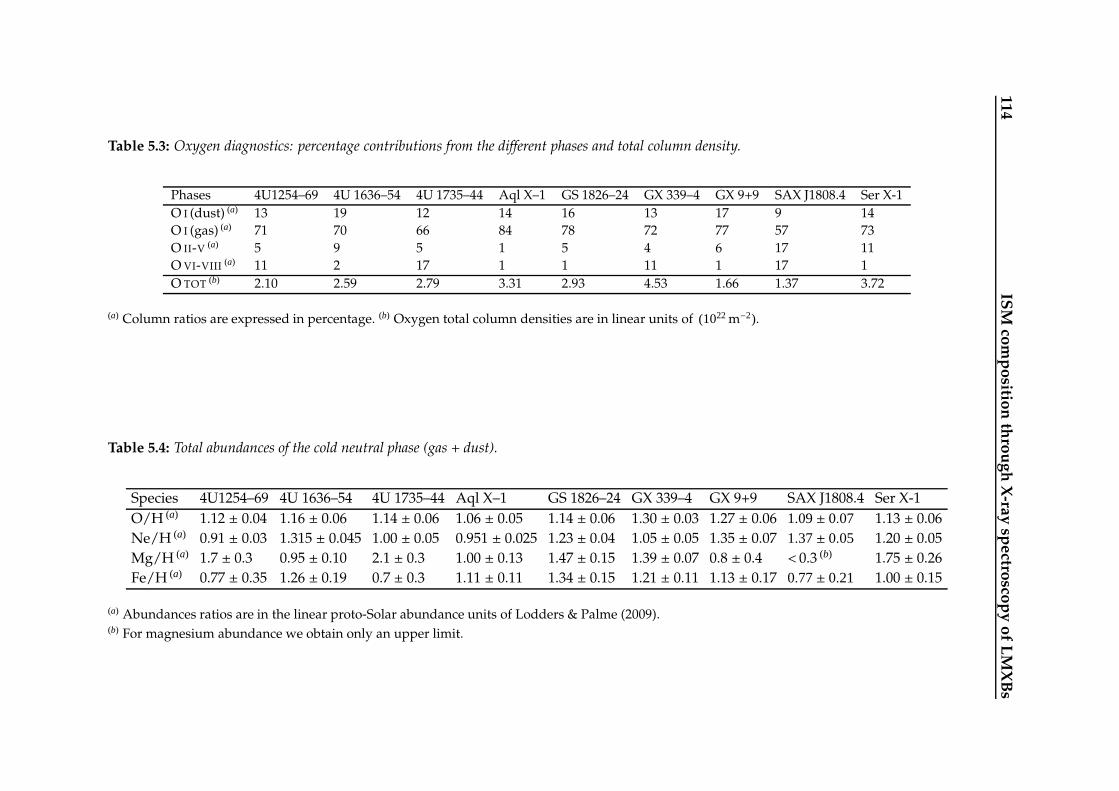
11
4IS
Mco
mp
ositio
nth
rou
gh
X-ra
ysp
ectro
scop
yo
fL
MX
Bs
Table 5.3: Oxygen diagnostics: percentage contributions from the different phases and total column density.
Phases 4U1254–69 4U 1636–54 4U 1735–44 Aql X–1 GS 1826–24 GX 339–4 GX 9+9 SAX J1808.4 Ser X-1
O I (dust) (a) 13 19 12 14 16 13 17 9 14
O I (gas) (a) 71 70 66 84 78 72 77 57 73
O II-V (a) 5 9 5 1 5 4 6 17 11
O VI-VIII (a) 11 2 17 1 1 11 1 17 1
O TOT (b) 2.10 2.59 2.79 3.31 2.93 4.53 1.66 1.37 3.72
(a) Column ratios are expressed in percentage. (b) Oxygen total column densities are in linear units of (1022 m−2).
Table 5.4: Total abundances of the cold neutral phase (gas + dust).
Species 4U1254–69 4U 1636–54 4U 1735–44 Aql X–1 GS 1826–24 GX 339–4 GX 9+9 SAX J1808.4 Ser X-1
O/H (a) 1.12 ± 0.04 1.16 ± 0.06 1.14 ± 0.06 1.06 ± 0.05 1.14 ± 0.06 1.30 ± 0.03 1.27 ± 0.06 1.09± 0.07 1.13 ± 0.06
Ne/H (a) 0.91 ± 0.03 1.315 ± 0.045 1.00 ± 0.05 0.951 ± 0.025 1.23 ± 0.04 1.05 ± 0.05 1.35 ± 0.07 1.37± 0.05 1.20 ± 0.05
Mg/H (a) 1.7 ± 0.3 0.95 ± 0.10 2.1 ± 0.3 1.00 ± 0.13 1.47 ± 0.15 1.39 ± 0.07 0.8 ± 0.4 < 0.3 (b) 1.75 ± 0.26
Fe/H (a) 0.77 ± 0.35 1.26 ± 0.19 0.7 ± 0.3 1.11 ± 0.11 1.34 ± 0.15 1.21 ± 0.11 1.13 ± 0.17 0.77± 0.21 1.00 ± 0.15
(a) Abundances ratios are in the linear proto-Solar abundance units of Lodders & Palme (2009).(b) For magnesium abundance we obtain only an upper limit.
5.6 Conclusion 115
5.6 Conclusion
We have presented a detailed treatment of the interstellar medium towards the nineLMXBs: GS 1826−238, GX 9+9, GX 339−4, Aql X−1, SAX J1808.4−3658, Ser X−1, 4U1254−690, 4U 1636−536, and 4U 1735−444. These bright X-ray sources are spread overabout 100 degrees in longitude and are located near the Galactic plane, which makesthem a very good workbench for a study focused on the ISM in the Galactic disk.
We probed the ISM dust composition, total abundances, and abundance gradients.We have shown that along these LOS the ISM is composed of a complex mixture ofa multi-phase gas, dust, and molecules. The analysis of all ionic species of oxygenshowed that the gas is mostly neutral. The column densities of the neutral gas speciesare in agreement with those found in the literature. The column densities that we es-timated for the mildly ionized gas are generally lower because previous work did nottake into account that a significant part of the ISM transmission may be provided bydust. Oxygen in solids is mostly provided by ices and silicates. About 15–20% and 70–90% of the total amount of neutral oxygen and iron, respectively, is found in dust. Thisresult provides a solution to the problem recently raised on the oxygen depletion andtotal abundance in the interstellar medium. Interestingly, the dust contribution andthe compounds mixture seem to be consistent along all the lines-of-sight (LOS). Theratios between the different ionization states are also similar between the LOS. Thissuggests that on a large scale the ISM is chemically homogeneous. Finally, using ourX-ray data we confirm the abundance gradients in the Galaxy and the local proto-Solarabundances as derived at longer wavelengths. Through the comparison between ourestimates of oxygen abundance and those obtained by other work on nearby youngstars and other indicators such as H II regions and planetary nebulae, we also confirmthat the local Galaxy is chemically homogeneous. This work shows that X-ray spec-troscopy is a very powerful method to probe the ISM.
Acknowledgements
This work is based on observations obtained with XMM-Newton, an ESA science mis-sion with instruments and contributions directly funded by ESA Member States andthe USA (NASA). SRON is supported financially by NWO, the Netherlands Organiza-tion for Scientific Research. We are grateful to Jean in’t Zand and Frank Verbunt for theuseful discussion about the physics and distances of the low-mass X-ray binaries.
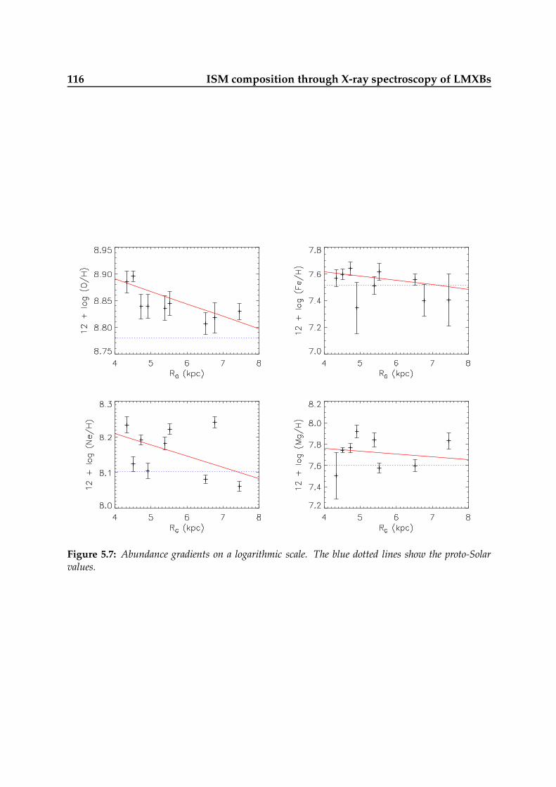
116 ISM composition through X-ray spectroscopy of LMXBs
Figure 5.7: Abundance gradients on a logarithmic scale. The blue dotted lines show the proto-Solarvalues.
Chapter 6
Conclusions & Prospects
The interstellar medium (ISM) is the ideal partner of the stars in the evolutionary cycleof the Galaxy. Heavy elements from carbon to uranium are produced by stellar evo-lution and are released in the surrounding ISM. Part of the interstellar (IS) matter isused to give birth to new stars. Abundances of heavy elements in the ISM are there-fore important to probe the past stellar evolution. However, the IS abundances arestill to be accurately determined, even for the most abundant metals such as Fe and O.Strong systematic uncertainties are due to the unknown detailed chemical compositionof these elements which are significantly depleted in dust. Therefore this thesis aimsto provide a successful method to measure the amounts of metals and dust in the ISMthrough observations of their absorption lines in X-ray spectra of background sources.
6.1 Structure and homogeneity of the diffuse ISM
In the previous chapter we have shown that X-ray absorption spectroscopy is a pow-erful tool to investigate the ISM. Through the study of its absorption lines in the X-rayspectra of background sources like active galactic nuclei (AGN) and X-ray binaries itwas indeed possible to measure column densities for several molecular, atomic, andionized gas species for heavy elements like C, N, O, Ne, Mg, Si, and Fe. Once we tookinto account all the contributions from dust and gas, we have accurately determinedthe total abundances for the cold interstellar phase. We also determined abundancegradients in the Galaxy for interstellar O, Ne, Mg, and Fe. They were consistent withabundances gradients estimated with different methods (see e.g. Chapter 2, 4, and 5).Briefly, all the abundances increase towards the center of the Galaxy confirming thatstellar evolution proceeds faster in the inner regions of the Galaxy. However, the gra-dients generally differ between the various elements, which suggests that the ratios
118 Conclusions & Prospects
between the contributions to ISM metal enrichment provided by giant evolved starsand supernovae vary within the Galaxy. A thorough dedicated study to this field isrequired in order to provide more accurate estimates. However, we have confirmedthat along any line-of-sight (LOS) the diffuse ISM is composed of a complex mixture ofa multi-phase gas and dust. The analysis of all ionic species of oxygen showed that thegas is mostly neutral. Oxygen in solids is mostly provided by ices and silicates. About15–20% and 70–90% of the total amount of neutral oxygen and iron, respectively, isfound in dust. This result provides a solution to the problem recently raised on the oxy-gen depletion and total abundance in the ISM. Interestingly, the dust contribution andthe compounds mixture seem to be consistent along any LOS. The ratios between thedifferent ionization states do not strongly vary within the Galactic disk. This suggeststhat on a large scale the ISM is chemically homogeneous. Finally, through the compar-ison between our estimates of IS oxygen abundance and those obtained by other workon nearby young stars and other indicators such as H II regions and planetary nebulae,we also confirm that the local Galaxy is chemically homogeneous.
6.2 Distinguishing clouds in the ISM, CGM, and IGM
The multiwavelength analysis provides us with an even more interesting workbenchfor the study of the ISM. For Instance, the combined UV and X-ray spectroscopy ofbackground AGN allows to search for clouds that belong to the circumgalactic (CGM)or to the intergalactic (IGM) medium. The study of these clouds probes the evolutionof the Galactic halo and its interaction with the surrounding CGM. In Chapter 4 wehave presented a complete analysis of the interstellar and circumgalactic medium to-wards the bright AGN Mrk 509 through high-quality spectra taken with XMM-Newton,Hubble Space Telescope, and FUSE. We have detected and analyzed seven different cloudsystems along this LOS. The single low- and three intermediate-velocity clouds (LVCand IVCs, v . 100km/s) are characterized by three distinct main phases with differ-ent ionization states. The high-velocity clouds (HVCs, v & 100km/s), which usuallyprobe the Galactic halo and the CGM, have a different structure and in the LOS to-wards Mrk 509 they show just two ionized phases. They are highly ionized most likelyas the result of the large exposure to the X-ray background and the interaction withthe circumgalactic medium. The similar abundances and ionization structure suggesta common origin for these HVCs. They may be at the outskirt of an extragalactic cloudcaptured by the Galaxy. The LVC and one of the IVCs belong to interstellar gas co-rotating with the Galactic disk, as confirmed by the detection of dust and molecules atrest wavelengths. The location of two other IVCs is not well constrained, they mightbelong either to disk co-rotating gas or to Galactic fountains. The most accepted sce-nario suggests that LVCs represent gas commonly found in the Galactic disk, IVCsmostly indicate Galactic fountains, while HVCs originate in the extragalactic environ-ment and are captured by the Galactic gravitational field. Extending this work to moreLOS would give a reply to many open questions concerning the origin of these cloudsand their effects on the metallicity of the Galactic ISM.
6.3 Nova ejecta and CSM 119
6.3 Nova ejecta and CSM
Stars enrich with metals the ISM, but the ratios between the metallic yields providedby certain types of stars are not yet well determined. Models of stellar evolution andmetallic yields are not always in agreement. The observations can provide accurate andalternative results through which is possible to discriminate between different evolu-tionary models. Novae are an interesting subclass of cataclysmic variables consisting ofan exploding white dwarf (WD) that pulls out its metal-rich matter in the surroundingmedium. In Chapter 3 we have reported our analysis of the XMM-Newton spectrumof nova V2491 Cyg and showed that its ejecta are well described by highly (photo-)ionized and metal-rich expanding shells. Their abundances indicate that they wereejected from an O-Ne white dwarf. Cold circumstellar and interstellar matter includ-ing dust is also present. High abundances of O and N shows that the surroundingmedium is significantly enriched with metals by the nova ejecta. Variations on timescales of hours occur both in the luminosity of the central source and in the ionizationlevel and columns of the absorption shells. The expanding gas is responding almostinstantaneously to the variations in the source ionizing continuum. This work is apioneer, new approach to the study of nova ejecta and might provide a powerful al-ternative method to probe their interaction with the surrounding medium and theirrole in the enrichment of metals. There are several nova spectra in the archive of theChandra and XMM-Newton satellites onto which this analysis can be easily extended.This will provide important information on the structure and chemistry of nova ejectaand their effects on the metallicity of the surrounding medium.
6.4 Prospects
It is worth to say that we are in the golden age of the ISM X-ray spectroscopy. The cur-rent and future X-ray satellites allow for accurate measurements of interstellar columndensities, ionization states, depletion factors, abundances, and dynamics, which areuseful to determine the chemical and physical states of all the phases of the ISM. Thisthesis is the first systematic, thorough study carried over this field and provided somepowerful methods useful to investigate the ISM. We also succeeded in solving some ofthe issues concerning the ISM composition and chemistry raised in Chapter 1. How-ever, it will be necessary to extend this work on a large scale involving more targetspointing to different Galactic regions and more instruments. More targets will providea mapping of the diffuse ISM and more accurate estimates of abundance gradients inthe Galaxy. More instruments, possibly also covering different energy domains suchas far-UV and X-ray, will provide independent measurements for same ionic species.Moreover, some energy regimes contain transitions from species which are missing atother energies (see e.g. Chapter 4).
The exact molecular composition of the cold IS phase is still an issue. Si, Mg, Fe,and O are among the elements that most contribute to the total mass of moleculargas and dust, but are often found in the same molecular compound. Therefore, thesimultaneous fits of their absorption edges respectively located at 6.7, 9.5, 17.5, and

120 Conclusions & Prospects
6.2 6.4 6.6 6.8 7
125
130
135
140
Pho
tons
m−
2 s−
1 Å
−1
Si K
13.5 14 14.54045
5055
60
Pho
tons
m−
2 s−
1 Å
−1
Wavelength (Å)
Ne IX
Ne K
Ne II−III
16.5 17 17.5 18
2025
3035
Wavelength (Å)
FeL2
FeL3
8.5 9 9.590
100
110
120
Mg XIMg K
Figure 6.1: Simulated spectrum of GS 1826–238 for a 100 ks observation with Astro-H/SXS.The spectral model refers to the (gas + dust) Model C as given in Chapter 2.
23.0 Å are required. No current instrument is provided with high effective area andspectral resolution at these wavelengths, simultaneously. Therefore, the contemporaryuse of the spectrometers on board different satellites will provide the best workbenchfor this analysis. For instance, Chandra/HETGS is the best detector at wavelengths upto the Fe L-edge (λ . 17.5 Å), while XMM-Newton/RGS is the most sensible near the OK-edge (λ ∼ 23.0 Å). Our working team at SRON is currently working on this multi-wavelength analysis and accurately measuring depletion factors and dust compositionfor both iron and oxygen (see e.g. Costantini et al. 2012).
The current X-ray satellites will be operating for most of this decade and a new X-ray mission (Astro-H, Takahashi et al. 2010) will be launched in two years from now.The soft X-ray Calorimeter Spectrometer (SXS) on board this satellite will combine forthe first time high sensitivity and spectral resolution in the broad 0.3 − 12keV energy
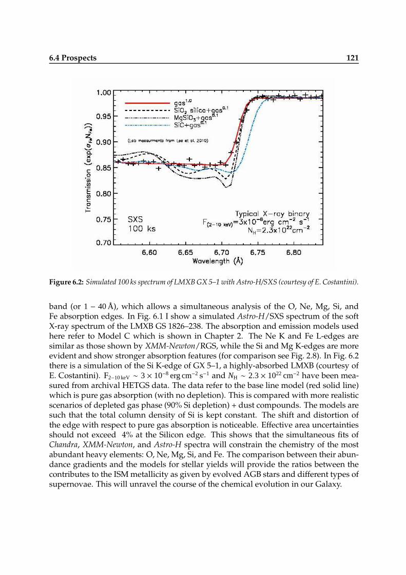
6.4 Prospects 121
Figure 6.2: Simulated 100 ks spectrum of LMXB GX 5–1 with Astro-H/SXS (courtesy of E. Costantini).
band (or 1 − 40 Å), which allows a simultaneous analysis of the O, Ne, Mg, Si, andFe absorption edges. In Fig. 6.1 I show a simulated Astro-H/SXS spectrum of the softX-ray spectrum of the LMXB GS 1826–238. The absorption and emission models usedhere refer to Model C which is shown in Chapter 2. The Ne K and Fe L-edges aresimilar as those shown by XMM-Newton/RGS, while the Si and Mg K-edges are moreevident and show stronger absorption features (for comparison see Fig. 2.8). In Fig. 6.2there is a simulation of the Si K-edge of GX 5–1, a highly-absorbed LMXB (courtesy ofE. Costantini). F2−10 keV ∼ 3× 10⁻⁸ erg cm−2 s−1 and NH ∼ 2.3× 1022 cm−2 have been mea-sured from archival HETGS data. The data refer to the base line model (red solid line)which is pure gas absorption (with no depletion). This is compared with more realisticscenarios of depleted gas phase (90% Si depletion) + dust compounds. The models aresuch that the total column density of Si is kept constant. The shift and distortion ofthe edge with respect to pure gas absorption is noticeable. Effective area uncertaintiesshould not exceed 4% at the Silicon edge. This shows that the simultaneous fits ofChandra, XMM-Newton, and Astro-H spectra will constrain the chemistry of the mostabundant heavy elements: O, Ne, Mg, Si, and Fe. The comparison between their abun-dance gradients and the models for stellar yields will provide the ratios between thecontributes to the ISM metallicity as given by evolved AGB stars and different types ofsupernovae. This will unravel the course of the chemical evolution in our Galaxy.

122 Conclusions & Prospects

Chapter 7
Nederlandse Samenvatting
Ons galactisch stelsel, ook wel bekend als “de Melkweg”, ziet eruit als een grote stadmet honderden miljarden sterren. De sterren zijn ingebed in een zeer ijl gas dat ”inter-stellair medium” (ISM) wordt genoemd. Het ISM bevat materie in de vorm van gas,stof en moleculen vergelijkbaar met sigarettenrook. Tijdens de oerknal werden alleenlichte elementen gevormd, zoals waterstof en helium, terwijl de meeste zwaardere ele-menten, zoals koolstof en uranium, later zijn gevormd door thermonucleaire explosiesin het binnenste van sterren. Dit proces, ook wel bekend als “sterevolutie”, verrijkt hetISM met metalen en moleculen. Uit een deel van de interstellaire (IS) materie ontstaannieuwe sterren, waarvan de chemische samenstelling verschilt van de vorige generatiesterren. Het ISM is dan ook de ideale partner van de sterren in de galactische evolu-tie en de hoeveelheid zware elementen in het ISM is een maat voor eerdere stellaireevolutie.
Rontgenspectroscopie is een krachtig instrument geworden om de chemische en fy-sische eigenschappen van het ISM te onderzoeken. In dit proefschrift presenteer ikeen succesvolle methode om de hoeveelheid metalen en stof in het ISM te meten doormiddel van observatie van hun absorptielijnen in de rontgenspectra van achtergronds-bronnen. Bijvoorbeeld, de hoeveelheid (of abundantie) van metalen neemt toe in derichting van het galactisch centrum, en dat duidt op een snellere ontwikkeling in debinnenste regionen.
7.1 De Melkweg en zijn ziel: het ISM
Het grootste deel van het zichtbare licht in de Melkweg wordt uitgezonden door ster-ren en wordt deels geabsorbeerd door een donker, koud interstellair (IS) stof dat inde buurt van het melkwegvlak ligt. Deze materie is bijna onzichtbaar voor het blote
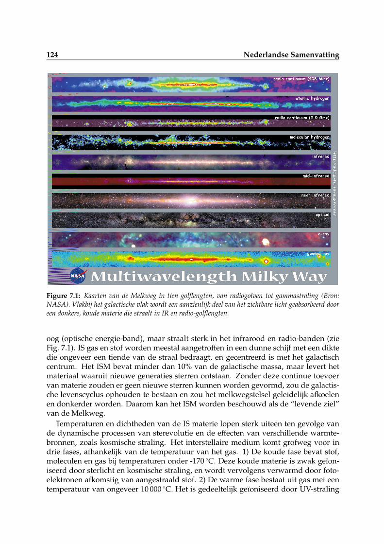
124 Nederlandse Samenvatting
Figure 7.1: Kaarten van de Melkweg in tien golflengten, van radiogolven tot gammastraling (Bron:NASA). Vlakbij het galactische vlak wordt een aanzienlijk deel van het zichtbare licht geabsorbeerd dooreen donkere, koude materie die straalt in IR en radio-golflengten.
oog (optische energie-band), maar straalt sterk in het infrarood en radio-banden (zieFig. 7.1). IS gas en stof worden meestal aangetroffen in een dunne schijf met een diktedie ongeveer een tiende van de straal bedraagt, en gecentreerd is met het galactischcentrum. Het ISM bevat minder dan 10% van de galactische massa, maar levert hetmateriaal waaruit nieuwe generaties sterren ontstaan. Zonder deze continue toevoervan materie zouden er geen nieuwe sterren kunnen worden gevormd, zou de galactis-che levenscyclus ophouden te bestaan en zou het melkwegstelsel geleidelijk afkoelenen donkerder worden. Daarom kan het ISM worden beschouwd als de “levende ziel”van de Melkweg.
Temperaturen en dichtheden van de IS materie lopen sterk uiteen ten gevolge vande dynamische processen van sterevolutie en de effecten van verschillende warmte-bronnen, zoals kosmische straling. Het interstellaire medium komt grofweg voor indrie fases, afhankelijk van de temperatuur van het gas. 1) De koude fase bevat stof,moleculen en gas bij temperaturen onder -170 C. Deze koude materie is zwak geıon-iseerd door sterlicht en kosmische straling, en wordt vervolgens verwarmd door foto-elektronen afkomstig van aangestraald stof. 2) De warme fase bestaat uit gas met eentemperatuur van ongeveer 10 000 C. Het is gedeeltelijk geıoniseerd door UV-straling

7.2 Verrijking van het ISM met metalen 125
van hete jonge sterren. 3) De hete fase is sterk geıoniseerd en verhit tot ongeveer 1miljoen C door schokgolven, die afkomstig zijn van supernova-explosies. Het wordtook wel “coronaal gas” genoemd, omdat de fysische toestand zeer vergelijkbaar is metdie van stercorona’s.
Hoewel het meeste ISM-licht wordt uitgezonden bij golflengten buiten de zichtbareband, is er een aantal interstellaire wolken die mooie figuren aan de hemel creeren.De zogenaamde paardenkopnevel is een wolkencomplex dat kenmerken van verschil-lende interstellaire fasen laat zien (zie Fig. 7.2). De koude en donkere stofwolken (metde vorm van een paardenkop) verduisteren het licht afkomstig van de achterliggendeemissienevel. De emissienevel bestaat uit warm geıoniseerd gas dat wordt verhit doorde nabijgelegen jonge sterren. De heldere blauwe nevels zijn wolken van interstellairstof die het licht van nabijgelegen sterren reflecteren. De energie van deze sterren isonvoldoende om het gas van de nevel te ioniseren zodat een emissienevel ontstaat,maar het is genoeg om stof zichtbaar te maken.
7.2 Verrijking van het ISM met metalen
Na de oerknal bestond de materie in het heelal alleen maar uit lichte elementen, zoalswaterstof (H), helium (He), lithium (Li) en beryllium (Be). Zwaardere elementen, zoalskoolstof en uranium (in de astronomie worden alle elementen zwaarder dan heliumook wel metalen genoemd), zijn later gevormd in de loop van de stellaire evolutiedoor nucleosynthese in de kernen van sterren. De chemische samenstelling van hetISM is vergelijkbaar met die van de zon: ongeveer 75% van de massa bestaat uit H,en 24% uit He. Hoewel de metalen slechts 1% van de totale massa uitmaken zijn zevan cruciaal belang om de chemische samenstelling en fysische toestand van het gas teverklaren.
Aggregaten bestaande uit stikstofatomen, moleculen en stof worden voornamelijkgevormd in geevolueerde middelzware (AGB) sterren. Elementen zwaarder dan Si(silicium), zoals Ca (calcium), Fe (ijzer) en Ni (nikkel) worden meestal door type Iasupernova’s (SN Ia) geproduceerd. Dit is een spectaculaire explosie van een wittedwergster, die geleidelijk massa opneemt van een begeleider tot het moment dat deontstekingstemperatuur voor koolstoffusie wordt bereikt. Binnen een paar secondenondergaat een aanzienlijk deel van de materie in de witte dwerg een kettingreactie,waarbij genoeg energie vrijkomt om de ster te laten exploderen als een supernova.Een type II supernova (SN II, ook wel supernova met kern-implosie genoemd) ontstaatuit de snelle ineenstorting en krachtige explosie van een zware ster. SN II producerenhet merendeel van de interstellaire zuurstof (O) en neon (Ne). Het gehalte aan zwareelementen is zodoende een directe afspiegeling van geschiedenis van de sterevolutie.In het jonge heelal is de verrijking van metalen sterk beınvloed door SN II, omdat eentype Ia supernova meer tijd nodig heeft om tot explosie te komen. Dit geeft aan dathet interstellaire gas in het begin verrijkt werd met elementen als zuurstof en silicium(Si). Later, toen SN Ia supernovae begonnen te exploderen, nam ook het gehalte vanzwaardere elementen zoals ijzer (Fe) en nikkel (Ni) in de ISM toe.
Zware elementen zoals koolstof, zuurstof, magnesium, silicium en ijzer zijn ook be-
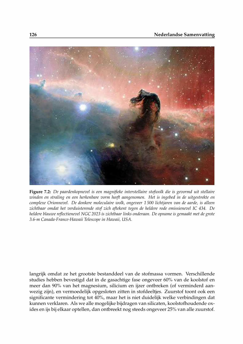
126 Nederlandse Samenvatting
Figure 7.2: De paardenkopnevel is een magnifieke interstellaire stofwolk die is gevormd uit stellairewinden en straling en een herkenbare vorm heeft aangenomen. Het is ingebed in de uitgestrekte encomplexe Orionnevel. De donkere moleculaire wolk, ongeveer 1 500 lichtjaren van de aarde, is alleenzichtbaar omdat het verduisterende stof zich aftekent tegen de heldere rode emissienevel IC 434. Deheldere blauwe reflectienevel NGC 2023 is zichtbaar links onderaan. De opname is gemaakt met de grote3.6-m Canada-France-Hawaii Telescope in Hawaii, USA.
langrijk omdat ze het grootste bestanddeel van de stofmassa vormen. Verschillendestudies hebben bevestigd dat in de gasachtige fase ongeveer 60% van de koolstof enmeer dan 90% van het magnesium, silicium en ijzer ontbreken (of verminderd aan-wezig zijn), en vermoedelijk opgesloten zitten in stofdeeltjes. Zuurstof toont ook eensignificante vermindering tot 40%, maar het is niet duidelijk welke verbindingen datkunnen verklaren. Als we alle mogelijke bijdragen van silicaten, koolstofhoudende ox-ides en ijs bij elkaar optellen, dan ontbreekt nog steeds ongeveer 25% van alle zuurstof.
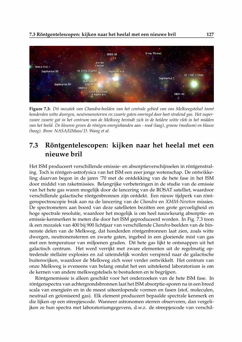
7.3 Rontgentelescopen: kijken naar het heelal met een nieuwe bril 127
Figure 7.3: Dit mozaıek van Chandra-beelden van het centrale gebied van ons Melkwegstelsel toonthonderden witte dwergen, neutronensterren en zwarte gaten omringd door heet stralend gas. Het super-zware zwarte gat in het centrum van de Melkweg bevindt zich in de heldere witte vlek in het middenvan het beeld. De kleuren geven de rontgen-energiebanden aan - rood (laag), groene (medium) en blauw(hoog). Bron: NASA/UMass/ D. Wang et al.
7.3 Rontgentelescopen: kijken naar het heelal met een
nieuwe bril
Het ISM produceert verschillende emissie- en absorptieverschijnselen in rontgenstral-ing. Toch is rontgen-astrofysica van het ISM een zeer jonge wetenschap. De ontwikke-ling daarvan begon in de jaren ’70 met de ontdekking van de hete fase in het ISMdoor middel van raketmissies. Belangrijke verbeteringen in de studie van de emissievan het hete gas waren mogelijk door de lancering van de ROSAT satelliet, waardoorverschillende galactische rontgenbronnen zijn ontdekt. Een nieuw tijdperk van ront-genspectroscopie brak aan na de lancering van de Chandra en XMM-Newton missies.De spectrometers aan boord van deze satellieten bezitten een grote gevoeligheid enhoge spectrale resolutie, waardoor het mogelijk is om heel nauwkeurig absorptie- enemissie-kenmerken te meten die door het ISM geproduceerd worden. In Fig. 7.3 toonik een mozaıek van 400 bij 900 lichtjaar van verschillende Chandra-beelden van de bin-nenste delen van de Melkweg, dat honderden rontgenbronnen laat zien, zoals wittedwergen, neutronensterren en zwarte gaten, ingebed in een gloeiende mist van gasmet een temperatuur van miljoenen graden. Dit hete gas lijkt te ontsnappen uit hetgalactisch centrum. Het werd verrijkt met zware elementen uit de regelmatig op-tredende stellaire explosies en zal uiteindelijk worden verspreid naar de galactischebuitenwijken, waardoor de Melkweg zich weer verder ontwikkelt. Het centrum vanonze Melkweg is eveneens van belang omdat het een uitstekend laboratorium is omde kernen van andere melkwegstelsels te bestuderen en te begrijpen.
Rontgenemissie is alleen geschikt voor het onderzoeken van de hete ISM fase. Inrontgenspectra van achtergrondsbronnen laat het ISM absorptie-sporen na in een breedscala van energieen en in de meest uiteenlopende vormen en fasen (stof, moleculen,neutraal en geıoniseerd gas). Elk element produceert bepaalde spectrale kenmerk endie lijken op een streepjescode. Wanneer astronomen sterren observeren, dan vergeli-jken ze hun spectra met laboratoriumgegevens, d.w.z. de streepjescode van verschil-
128 Nederlandse Samenvatting
lende elementen, zoals zuurstof, neon, magnesium en ijzer. Sterke pieken (emissieli-jnen) of diepe dalen (absorptielijnen) in de waargenomen spectra zijn karakteristiekvoor bepaalde elementen, en het is zo ook mogelijk om de hoeveelheid van elk elementaf te leiden (zie bijvoorbeeld Fig. 7.4). Absorptie-kenmerken van de ISM werden be-gin deze eeuw bij toeval ontdekt en wezen op de aanwezigheid van neutrale zuurstof,neon en ijzer. Speciale studies leidden tot de ontdekking van neutrale, enkelvoudigeen dubbel geıoniseerde atomen (vooral zuurstof en neon). De eerste metingen vande abundantieverhouding Fe/H in de ISM en hun vergelijking met de abundantiev-erhouding Fe/H van de zon lieten zien dat ijzer duidelijk ontbreekt (of verminderdaanwezig is) in de IS gasfase, en mogelijk is vastgelegd in stofdeeltjes. Complexe struc-turen nabij de K-absorptiekant van zuurstof laten zien dat zuurstof misschien voor eendeel zit opgesloten in IS stof of moleculen zoals hematiet, silicaten en ijs.
7.4 Dit proefschrift: doelen en resultaten
Het is duidelijk dat rontgenspectroscopie een belangrijk hulpmiddel is voor verder on-derzoek van het ISM. De huidige rontgensatellieten leveren nauwkeurige schattingenvan de hoeveelheid en ontbrekende fractie van metalen in de ISM en hun tempera-turen. Diverse open vragen moeten nog beantwoord worden. Wat is de moleculairesamenstelling van de koude interstellaire fase? Welke fractie van ieder element zit opgeslagenin stof? Verkeren bepaalde fasen in een zekere evenwichtstoestand en zo ja, welke? Wat zijn detotale abundanties van de elementen? Hoe verhouden al deze parameters zich tot het specifiekegalactische milieu? Hoe correleren abundantiepatronen in de Melkweg met de metaal-verrijkingdie door AGB sterren en supernovae worden geproduceerd? Dit proefschrift beantwoordteen aantal van deze vragen door middel van de analyse van de IS absorptielijnen inrontgenspectra van heldere achtergrondsbronnen.
Het diffuse ISM: structuur, samenstelling en homogeniteit
Ik heb IS absorptielijnen in de rontgenspectra van actieve galactische kernen (AGN) enrontgendubbelsterren bestudeerd, en ik heb gemeten welke fractie van de elementenC, N, O, Ne, Mg, Si en Fe aanwezig is in de vorm van moleculen, atomen en geıoniseerdgas. Het diffuse ISM is meestal samengesteld uit een complex mengsel van gas in di-verse fasen, stof en moleculen. De totale abundanties (gas + stof) van de koude IS fasenemen toe in de richting van het galactisch centrum, waaruit blijkt dat de stellaire evo-lutie in binnenste regionen van het melkwegstelsel sneller verloopt. In het algemeenverschilt de toenamesnelheid per element en dat suggereert dat de metaal-verrijkingvan het ISM door AGB sterren, SN I en SN II binnen het melkwegstelsel varieert. Stofis alomtegenwoordig en bevat ongeveer 15–20% van alle zuurstof en 70–90% van hetijzer. De hoeveelheid en samenstelling van stof lijkt constant te zijn in de galactischeschijf. Ongeveer 10% van het gas is geıoniseerd, en de verhouding tussen de verschil-lende ionisatietoestanden (die de temperatuur van elke fase bepalen) is ongeveer con-stant over de schijf. Dit suggereert dat het ISM op grote schaal chemisch homogeen is.Tot slot, de overeenstemming tussen de IS zuurstof abundantie en de gemeten waar-

7.4 Dit proefschrift: doelen en resultaten 129
050
010
00
Flu
x (
phot
ons
m−
2 s−
1 Å
−1
)
O V
III α
O V
III β
O V
III γ
O V
II α
O V
II β
O V
II ed
ge
SIL
ICA
TE
S
O V
II γ
O V
III e
dge
O I
N I
1s−
2p
C V
I α
N V
I αC
VI β
C V
I γ
N V
II α
O V
O V
I
N V
II β
N V
II γ
N V
I (f)
C V
I edg
e DAY 40.18
8 10 12 14
05
1015
Flu
x
Ne
IX
Ne
X
Mg
XI
Mg
XII
10 15 20 25 30 35
−10
010
χ
Wavelength (Å)
Figure 7.4: XMM-Newton spectrum van nova V2491 Cyg. De uitgestoten materie werd gemodelleerddoor schillen van foto-geıoniseerd gas met een snelheid van 3000 km/s. Let op de sterke absorptielijnenvan hoog-geıoniseerd O en N.
den voor nabijgelegen jonge sterren, H II gebieden en planetaire nevels, bevestigt datde Melkweg lokaal ook chemisch homogeen is.
Het lokale CSM en nova ejecta
De metaalproductie van bepaalde soorten sterren is nog steeds niet goed bekend. Ster-evolutie-modellen zijn niet altijd met elkaar in overeenstemming en soms leveren dewaarnemingen bruikbaardere resultaten. Nova’s zijn exploderende witte dwergster-ren (WD), die een deel van haar metaalrijke materie in het omringende circumstel-laire medium (CSM) blazen. Het XMM-Newton spectrum van nova V2491 Cyg lietzien dat de ejecta goed kunnen worden beschreven als schillen materie die met eensnelheid van 3000 km/s uitzetten, en die foto-geıoniseerd en verhit worden door deexploderende WD (zie Fig. 7.4). Absorptie door koud gas met lage snelheden (v <100km/s) vindt plaats in circumstellaire en interstellaire materie die stof bevat. Deabundanties van de schillen geven aan dat ze werden uitgeworpen door een O–Ne/N

130 Nederlandse Samenvatting
witte dwerg. De hoge O en N gehaltes in het koude absorberende gas laten zien dathet omringende medium aanzienlijk verrijkt is met metalen door de nova ejecta.
Verschillende omgevingen: ISM, CGM en IGM
Met spectraalanalyse in diverse golflengtegebieden (ultraviolet (UV) en rontgen) vanactieve galactische kernen (AGN) kan men ook wolken onderzoeken die deel uitmakenvan het circumgalactisch (CGM) of het intergalactisch medium (IGM), en hun interac-tie met de halo van de Melkweg. Ik heb het ISM en het CGM in de richting van deheldere AGN Mrk 509 geanalyseerd door middel van traliespectra van hoge-kwaliteitgenomen met XMM-Newton (rontgen), de Hubble Space Telescope en FUSE (UV-band).Langs de gezichtslijn liggen zeven complexe wolkensystemen. De hoge-snelheid wolk-en (v & 100km/s) zijn sterk geıoniseerd, waarschijnlijk ten gevolge van botsing met degalactische halo en een grotere blootstelling aan de rontgen-achtergrondstraling. Hunabundanties en ionisatie-structuur zijn vergelijkbaar, hetgeen suggereert dat zij zichmogelijk bevinden op de rand van een enkele extragalactische wolk (zie Fig. 7.5). Dewolken met een lage en middelmatige snelheid (v . 100km/s) bestaan zeer waarschi-jnlijk uit interstellair gas dat mee-roteert met de galactische schijf.
7.5 Vooruitzichten
We bevinden ons in de gouden eeuw van de ISM rontgenspectroscopie. De huidige entoekomstige rontgensatellieten zorgen voor nauwkeurige metingen van de tempera-turen, de hoeveelheid en samenstelling van het stof, de metaalabundanties en de snel-heden die de chemische en fysische structuur van het ISM bepalen. Dit proefschrift isde eerste systematische, grondige studie uitgevoerd op dit gebied en presenteert eenkrachtige methode om het ISM te onderzoeken. Het is echter noodzakelijk om dit werkgrootschaliger op te zetten met meerdere gezichtslijnen (d.w.z. meer bronnen) en ver-schillende instrumenten om het ISM nog beter in kaart te brengen, en nauwkeurigeschattingen van abundantiepatronen in de Melkweg te verkrijgen. De huidige ront-gensatellieten zullen voor het merendeel van dit decennium operationeel zijn, en denieuwe rontgenmissie Astro-H zal binnen twee jaar worden gelanceerd. De soft X-rayCalorimeter Spectrometer aan boord van deze satelliet zal voor het eerst een hoge spec-trale resolutie in een brede energieband van 0.3 tot 12keV (or 1− 40 Å), in combinatiemet een hoge gevoeligheid, waardoor een gelijktijdige analyse van de Fe, Ne, Mg enSi spectra mogelijk wordt. Samen met Chandra en XMM-Newton zal Astro-H de chemievan zware elementen zoals O, Mg, Si en Fe ontrafelen. De vergelijking van hun abun-dantiepatronen met de modellen van stellaire evolutie zal onthullen hoe het ISM isverrijkt met metalen van AGB sterren en verschillende soorten supernova’s. En hier-mee wordt het verloop van de chemische evolutie van ons melkwegstelsel vastgelegd.
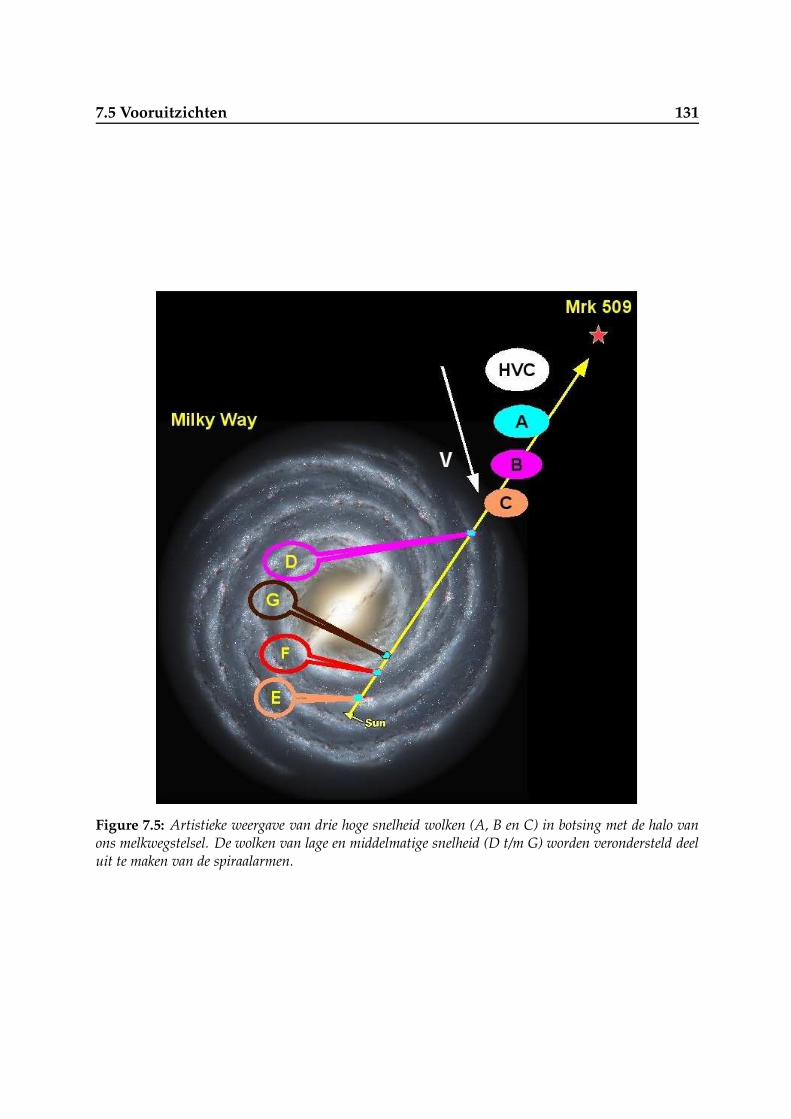
7.5 Vooruitzichten 131
Figure 7.5: Artistieke weergave van drie hoge snelheid wolken (A, B en C) in botsing met de halo vanons melkwegstelsel. De wolken van lage en middelmatige snelheid (D t/m G) worden verondersteld deeluit te maken van de spiraalarmen.

132 Nederlandse Samenvatting
Chapter 8
Sommario italiano
La nostra Galassia, nota anche come “Via Lattea”, si presenta come una grande cittadove vivono centinaia di miliardi di stelle. Le stelle sono circondate da nubi moltorade detto “mezzo interstellare” (ISM). L’ISM contiene materia sotto forma di gas epolvere simile al fumo di sigaretta. Il Big Bang ha creato solo gli elementi leggericome l’idrogeno e l’elio nei primi istanti di vita dell’Universo, mentre la maggior partedegli elementi piu pesanti dal carbonio all’uranio sono stati prodotti in seguito du-rante le reazioni termonucleari nei nuclei delle stelle. Questo processo, noto anchecome evoluzione stellare, ha arricchito l’ISM di metalli e molecole. Parte della materiainterstellare viene poi utilizzata per generare nuove stelle la cui composizione chimicadifferisce da quella delle precedenti generazioni. L’ISM e quindi il partner ideale dellestelle nell’evoluzione Galattica e la quantita di elementi pesanti nell’ISM sono la tes-timonianza dell’evoluzione stellare precedente. Tuttavia, nonostante i numerosi studisull’ISM, la sua composizione chimica non e stata ancora determinata con accuratezza.
La spettroscopia a raggi X e diventata un potente strumento per studiare le proprietachimiche e fisiche dell’ISM. In questa tesi mostro infatti un metodo efficace per mis-urare le quantita di metalli e polvere nell’ISM attraverso l’osservazione delle loro righedi assorbimento negli spettri a raggi X di sorgenti di fondo. Per esempio, la quantita(o abbondanza) di metalli risulta aumentare verso il centro della Galassia indicandoun’evoluzione piu veloce nelle sue regioni interne.
8.1 La Galassia e la sua anima: l’ISM
La maggior parte della luce visibile nella Via Lattea e emessa dalle stelle e viene inparte assorbita da una polvere interstellare oscura e fredda che si trova in prossimitadel piano galattico. Questa materia e quasi invisibile all’occhio nudo (banda di energia

134 Sommario italiano
Figure 8.1: Mappe della Via Lattea a dieci lunghezze d’onda, dalle onde radio ai raggi gamma (Credito:NASA). In prossimita del piano galattico una frazione significativa della luce ottica viene assorbita dauna materia oscura e fredda che emette a lunghezze d’onda infrarosse e radio.
ottica), ma emette fortemente nelle bande infrarosse e radio (vedi in Fig. 8.1). Gas epolveri interstellari si trovano principalmente all’interno di un disco sottile, il cui cen-tro concide con quello della Galassia. Questo disco gassoso viene detto sottile in quantoil suo spessore e circa 10 volte piu piccolo del suo raggio. L’ISM contiene meno del 10%della massa galattica, ma fornisce la fonte di materia per le nuove generazioni di stelle.Senza questo continuo apporto di materia nessuna nuova stella verrebbe creata, il ciclodi vita galattica si fermerebbe, e la Galassia si spegnerebbe progressivamente. Pertanto,l’ISM puo essere considerato come l’anima vivente della Galassia.
La materia interstellare possiede temperature e densita molto varie, che sono dovuteai diversi processi dinamici di evoluzione stellare e agli effetti di diverse fonti di calore,come ad esempio i raggi cosmici. Tuttavia, la maggior parte della materia si strutturain tre fasi caratteristiche, ognuna delle quali con un certo regime di temperatura.1) La fase fredda contiene polvere e gas a temperature inferiori a circa -170 C. Questamateria fredda e debolmente ionizzato dalla luce delle stelle e dei raggi cosmici e vienepoi riscaldata da fotoelettroni irradiati dalla polvere.2) La fase tiepida e costituita da gas con temperature di circa 10 000C. Essa e in partefotoionizzata dall’emissione UV di stelle giovani e calde.
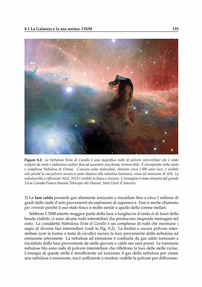
8.1 La Galassia e la sua anima: l’ISM 135
Figure 8.2: La Nebulosa Testa di Cavallo e una magnifica nube di polvere interstellare che e statascolpita da venti e radiazioni stellari fino ad assumere una forma riconoscibile. E incorporata nella vastae complessa Nebulosa di Orione. L’oscura nube molecolare, distante circa 1 500 anni luce, e visibilesolo perche la sua polvere oscura si pone dinanzi alla nebulosa luminosa, rossa ad emissione IC 434. Lanebulosa blu a riflessione NGC 2023 e visibile in basso a sinistra. L’immagine e stata ottenuta dal grande3,6 m Canada-France-Hawaii Telescope alle Hawaii, Stati Uniti d’America.
3) La fase calda possiede gas altamente ionizzato e riscaldato fino a circa 1 milione digradi dalle onde d’urto provenienti da esplosioni di supernova. Esso e anche chiamatogas coronale perche il suo stato fisico e molto simile a quello delle corone stellari.
Sebbene L’ISM emette maggior parte della luce a lunghezze d’onda al di fuori dellabanda visibile, ci sono alcune nubi interstellari che producono stupende immagini nelcielo. La cosiddetta Nebulosa Testa di Cavallo e un complesso di nubi che mostrano isegni di diverse fasi interstellari (vedi la Fig. 8.2). La fredda e oscura polvere inter-stellare (con la forma a testa di cavallo) oscura la luce proveniente dalla nebulosa ademissione retrostante. La nebulosa ad emissione e costituita da gas caldo ionizzato eriscaldato dalla luce proveniente da stelle giovani e calde nei suoi pressi. Le luminosenebulose blu sono nubi di polvere interstellare che riflettono la luce delle stelle vicine.L’energia di queste stelle e insufficiente ad ionizzare il gas della nebulosa per creareuna nebulosa a emissione, ma e sufficiente a rendere visibile la polvere per diffusione.

136 Sommario italiano
8.2 Arricchimento di metalli dell’ISM
Il Big Bang diede origine soltanto agli elementi leggeri come idrogeno (H), elio (He),litio (Li) e berillio (Be). Elementi piu pesanti come quelli dal carbonio all’uranio (inastronomia tutti gli elementi piu pesanti dell’elio sono spesso chiamati metalli) sonostati formati dopo nel corso dell’evoluzione stellare attraverso la nucleosintesi nei nu-clei stellari. La composizione chimica dell’ISM e simile a quella del Sole: circa il 75%e il 24% in massa vengono forniti da H ed He, rispettivamente. Sebbene i metalli con-tengono solo il restante 1% della massa totale, essi sono cruciali per comprendere lacomposizione chimica e lo stato fisico del gas.
Azoto atomico, molecole e polveri si formano principalmente in stelle evolute dimedia massa (stelle AGB). Gli elementi piu pesanti del silicio, come ad esempio calcio,ferro e nichel, sono principalmente forniti dalla supernova di tipo Ia (SN Ia). Si trattadi una violenta esplosione di una nana bianca che accresce a poco a poco materia dauna stella compagna fino al punto in cui si raggiunge la temperatura sufficiente adinnescare la fusione di carbonio. Nel giro di pochi secondi una frazione sostanzialedella materia della nana bianca subisce una reazione a catena, rilasciando energia suf-ficiente ad esplodere la stella in una supernova. Un supernova di tipo II (SN II, notaanche come supernova a collasso nucleare) rappresenta il rapido collasso e l’esplosioneviolenta di una stella massiccia. Supernove di questo tipo forniscono la maggior partedell’ossigeno e del neon interstellari. Pertanto, e chiaro che gli elementi pesanti testi-moniano direttamente la storia della passata evoluzione stellare. Nei primi anni di vitadell’Universo, l’arricchimento di metalli e stato guidato dalle SN II, perche il tipo Iarichiede molto piu tempo per esplodere. Questo indica che il gas interstellare e statodapprima arricchito di elementi come ossigeno e silicio. Successivamente, quando leSN Ia hanno iniziato a esplodere, gli elementi piu pesanti come il ferro e nichel sonodivenuti piu abbondanti.
Carbonio, ossigeno, magnesio, silicio e ferro sono anche importanti perche con-tengono la maggior parte della massa in polvere. Diversi studi hanno confermatoche circa il 60% di carbonio e piu del 90% di magnesio, silicio e ferro mancano (osono esauriti) nella fase gassosa e sono presumibilmente rinchiusi in granuli di pol-vere. L’ossigeno mostra fattori di esaurimento fino al 40%, ma non si capisce benequali composti molecolari possano giustificare tali valori. Se sommiamo tutti i pos-sibili contributi forniti da silicati, ossidi di carbonio e ghiacci, c’e ancora un 25% diossigeno mancante (se confrontati con l’abbondanza di ossigeno nel sistema solare).
8.3 Telescopi a raggi X: nuovi occhi puntati sull’Universo
Nei raggi X l’ISM produce svariati fenomeni di emissione ed assorbimento, tuttavial’astrofisica nei raggi X dell’ISM e una scienza molto giovane, il cui sviluppo e in-iziato con la scoperta della fase interstellare calda negli anni ’70 attraverso il lancio dirazzi e satelliti muniti di rivelatori per raggi X. Miglioramenti importanti nello studiodell’emissione del gas caldo sono stati forniti dal lancio del satellite ROSAT, che ha por-tato alla scoperta di diverse sorgenti galattiche di raggi X. Dopo il lancio delle missioni

8.3 Telescopi a raggi X: nuovi occhi puntati sull’Universo 137
Figure 8.3: Questo mosaico di immagini Chandra della regione centrale della nostra Galassia rivelacentinaia di nane bianche, stelle di neutroni e buchi neri circondati da gas caldo in emissione. Il buconero al centro della Galassia si trova all’interno della chiazza bianca e luminosa nel centro dell’immagine.I colori indicano bande di energia di raggi X - rosso (bassa), verde (media) e blu (alta). Credito: NASA /UMass / D.Wang et al.
Chandra e XMM-Newton una nuova era per la spettroscopia a raggi X e stata inaugu-rata. Gli spettrometri a bordo di questi satelliti sono dotati di sensibilita e risoluzionespettrale elevate in grado di misurare con precisione profili di assorbimento ed emis-sione prodotti dall’ISM. In Fig. 8.3 mostro un mosaico di 400 x 900 anni luce di diversiimmagini Chandra delle regioni piu interne della Via Lattea, che rivela centinaia di sor-genti di raggi X, come nane bianche, stelle di neutroni e buchi neri incorporati in unanebbia incandescente di gas di svariati milioni gradi. Questo gas caldo sembra esserein fuga dal centro galattico. Il gas e stato arricchito di elementi pesanti dalla frequentedistruzione stellare e li distribuira nei sobborghi del sistema galattico influenzandonel’evoluzione. Il centro della nostra Galassia e importante anche perche fornisce uneccellente laboratorio per conoscere i nuclei di altre galassie.
Tuttavia, lo studio dell’emissione di raggi X e adatto solo per sondare la fase caldadell’ISM. Negli spettri a raggi X delle sorgenti di fondo le varie forme e fasi inter-stellari (polvere, molecole, gas atomico e ionizzato) producono profili di assorbimentoper una vasta gamma di energie. Ogni elemento produce una certa quantita di traccespettrali simili ad un codice a barre. Quando gli astronomi osservano le stelle, con-frontano i loro spettri con quelli presi in laboratorio per diversi tipi di elementi comeossigeno, neon, magnesio e ferro (i suddetti “codici a barre”). Intensi picchi (noti comerighe di emissione) o avvallamenti (righe di assorbimento) negli spettri osservati sonoquindi identificati come le tracce lasciate da certi elementi. Dalle loro intensita e an-che possibile ricavare la quantita di ciascun elemento (si veda ad esempio la Fig. 8.4).Nei primi “anni 2000”, profili e righe di assorbimento vennero scoperti per caso e riv-elarono la presenza di ossigeno, neon e ferro neutri nell’ISM. Studi accurati hannoportato alla scoperta di molte specie neutre e ionizzate (per lo piu di ossigeno e neon).Le prime misure dei rapporti di abbondanza tra ferro e idrogeno nell’ISM e succes-sivo confronto con i rispettivi valori solari ha dimostrato che il ferro e significativa-mente mancante (o esaurito) nella fase interstellare gassosa e, eventualmente, rinchiusoin granuli di polvere. Strutture complesse scoperte vicino al profilo di assorbinento
138 Sommario italiano
della shell K dell’ossigeno hanno mostrato che una parte significativa dell’ossigeno in-terstellare potrebbe essere immagazzinata in polvere o molecole come ematite, silicatie ghiacci.
8.4 Questa tesi: obiettivi e risultati
E chiaro che la spettroscopia a raggi X fornisce un banco di lavoro importante perstudiare l’ISM. Gli attuali satelliti a raggi X consentono stime accurate di metallicita,temperature, e fattori di esaurimento. Molte sono le domande ancora aperte in questocampo di ricerca. Qual e la composizione molecolare della fase interstellare fredda? Qual e lapercentuale in polvere di ogni elemento? Ogni fase e in uno certo stato di equilibrio, se si quale?Quali sono le abbondanze totali degli elementi? Come si relazionano tutti questi parametricon lo specifico contesto galattico? Come correlano i gradienti di abbondanza nella Galassiacon l’arricchimento di metalli fornito da stelle AGB e supernove? Questa tesi risponde adalcune di queste domande attraverso l’analisi di righe di assorbimento interstellarenegli spettri dei raggi X di sorgenti luminose di fondo.
ISM diffuso: struttura, composizione e omogeneita
Ho studiato righe di assorbimento interstellare negli spettri di raggi X di nuclei galatticiattivi (AGN) e binarie di fondo ed ho misurato le quantita di gas molecolare, atomicoe ionizzato per svariate forme di C, N, O, Ne, Mg, Si e Fe. L’ISM diffuso e general-mente composto da una miscela complessa di gas multi-fase e polveri. Tutte le ab-bondanze totali (gas + polvere) della fase fredda aumentano verso il centro galattico eindicano che l’evoluzione stellare procede piu velocemente nelle regioni interne dellaGalassia. I gradienti delle abbondanze dei vari elementi sono generalmente diversi esuggeriscono che i contributi arricchimento di metalli nell’ISM forniti da stelle AGB,SN Ia e SN II variano all’interno della Galassia. La polvere e sempre presente nel discogalattico e contiene circa il 15–20% e il 70–90% di ossigeno e ferro, rispettivamente. Laquantita e la composizione della polvere interstellare sembrano non variare all’internodi tale disco. Circa il 10% del gas e ionizzato, ma i rapporti tra le quantita di gastrovato ai diversi stati di ionizzazione sono simili attraverso il disco, essi fornisconola temperatura di ciascuna fase. Questo suggerisce che su larga scala l’ISM diffusoe chimicamente omogeneo. Infine, l’accordo tra la abbondanza di ossigeno interstel-lare e il lavore misurato per giovani stelle, regioni h II e le nebulose planetarie vicineconferma che localmente anche la Galassia e chimicamente omogenea.
CSM locale e materia espulsa intorno ad una nova
Il rendimento in metalli fornito da alcuni tipi di stelle non e stato ancora ben de-terminato. I modelli di evoluzione stellare non sono sempre consistenti e qualchevolta le osservazioni possono fornire risultati piu precisi ed alternativi. Le cosid-dette stelle nove consistono di una nana bianca che esplode ed espelle parte dellasua materia ricca di metalli nel mezzo circumstellare circostante (CSM). Lo spettro
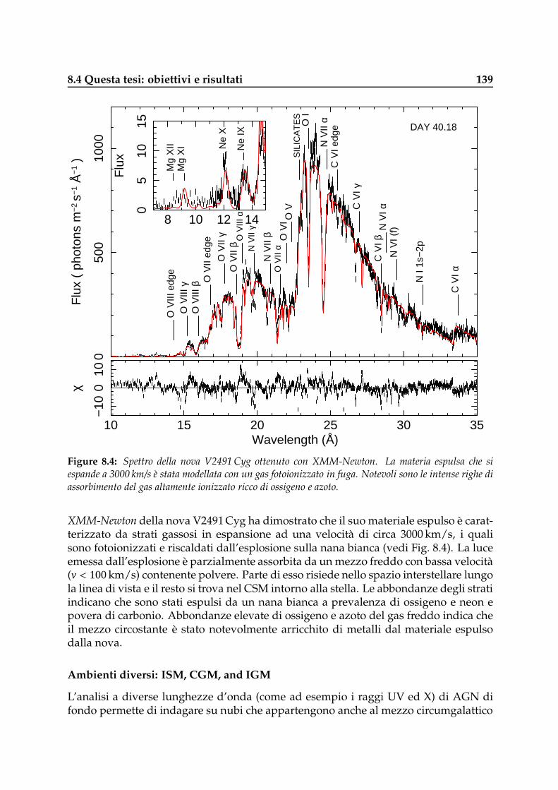
8.4 Questa tesi: obiettivi e risultati 139
050
010
00
Flu
x (
phot
ons
m−
2 s−
1 Å
−1
)
O V
III α
O V
III β
O V
III γ
O V
II α
O V
II β
O V
II ed
ge
SIL
ICA
TE
S
O V
II γ
O V
III e
dge
O I
N I
1s−
2p
C V
I α
N V
I αC
VI β
C V
I γ
N V
II α
O V
O V
I
N V
II β
N V
II γ
N V
I (f)
C V
I edg
e DAY 40.18
8 10 12 14
05
1015
Flu
x
Ne
IX
Ne
X
Mg
XI
Mg
XII
10 15 20 25 30 35
−10
010
χ
Wavelength (Å)
Figure 8.4: Spettro della nova V2491 Cyg ottenuto con XMM-Newton. La materia espulsa che siespande a 3000 km/s e stata modellata con un gas fotoionizzato in fuga. Notevoli sono le intense righe diassorbimento del gas altamente ionizzato ricco di ossigeno e azoto.
XMM-Newton della nova V2491 Cyg ha dimostrato che il suo materiale espulso e carat-terizzato da strati gassosi in espansione ad una velocita di circa 3000 km/s, i qualisono fotoionizzati e riscaldati dall’esplosione sulla nana bianca (vedi Fig. 8.4). La luceemessa dall’esplosione e parzialmente assorbita da un mezzo freddo con bassa velocita(v < 100km/s) contenente polvere. Parte di esso risiede nello spazio interstellare lungola linea di vista e il resto si trova nel CSM intorno alla stella. Le abbondanze degli stratiindicano che sono stati espulsi da un nana bianca a prevalenza di ossigeno e neon epovera di carbonio. Abbondanze elevate di ossigeno e azoto del gas freddo indica cheil mezzo circostante e stato notevolmente arricchito di metalli dal materiale espulsodalla nova.
Ambienti diversi: ISM, CGM, and IGM
L’analisi a diverse lunghezze d’onda (come ad esempio i raggi UV ed X) di AGN difondo permette di indagare su nubi che appartengono anche al mezzo circumgalattico

140 Sommario italiano
Figure 8.5: Vista artistica di tre nubi ad alta velocita (A-to-C) che impattano l’alone galattico. In questoscenario le nubi a bassa e media velocita (D-to-G) appartengono a bracci di spirale della Galassia.
(CGM) o intergalattico (IGM) e sulla loro interazione con l’alone galattico. Ho anal-izzato l’ISM e il CGM verso il luminoso AGN Mrk 509 con spettri di elevata qualitaottenuti con XMM-Newton (nei raggi X), Hubble Space Telescope e FUSE (nella bandaUV). Sette sistemi complessi di nubi si trovano lungo questa linea di vista. Le nubiad alta velocita (v & 100km/s) sono altamente ionizzate molto probabilmente a causadell’elevata esposizione al fondo di raggi X e dell’interazione collisionale con l’alonegalattico. Le loro abbondanze e gradi di ionizzazione simili suggeriscono che potreb-bero trovarsi nella periferia di una nube extragalattica (vedi Fig. 8.5). Le nubi a bassae media velocita (v . 100km/s) sono piu probabilmente gas interstellare che ruota conil disco galattico.
8.5 Prospettive per il futuro 141
8.5 Prospettive per il futuro
Ci troviamo nell’eta d’oro della spettroscopia a raggi X del mezzo interstellare. I satellitia raggi X attuali e futuri consentono di misurare con precisione temperature, quantitae composizione in polvere, abbondanze metalliche e dinamiche delle nubi interstellariovvero quei parametri che determinano la struttura chimica e fisica dell’ISM. Questatesi e il primo studio sistematico ed approfondito svolto in questo settore e fornisce unmetodo efficace per studiare l’ISM. Tuttavia, e necessario estendere questo lavoro suuna larga scala che coinvolga piu linee di vista (ovvero piu sorgenti) e diversi strumentiper una mappatura migliore dell’ISM e per stime accurate dei gradienti di abbondanzaall’interno della Galassia. Gli attuali satelliti a raggi X saranno operativi per la maggiorparte di questo decennio e la nuova missione nei raggi X Astro-H sara lanciata in dueanni a partire da adesso. Lo spettrometro a calorimetro nei raggi X a bordo di questosatellite fornira per la prima volta un’alta risoluzione spettrale nella banda di energia0, 3 − 12keV (ovvero 1 − 40 Å) combinata con un’elevata sensibilita e la possibilita diuna analisi simultanea di Fe, Ne, Mg e Si. Insieme a Chandra ed XMM-Newton, Astro-Hsbrogliera la chimica di elementi pesanti come O, Mg, Si e Fe. Il confronto tra i lorogradienti di abbondanza ed i modelli di evoluzione stellare riveleranno come l’ISMe stato arricchito di metalli dalle stelle AGB e dai diversi tipi di supernove. Questolavoro descrivera il corso dell’evoluzione chimica della nostra Galassia.

142 Sommario italiano
Appendix A
Appendix to Chapter 2: Absorption byoxygen molecules
The amol model calculates the transmission of various molecules. Presently only theoxygen edge is taken account of. Updates of this model, once made, will be reported inthe manual of SPEX. The following compounds are presently taken into account (seeTable A.1).
The chemical composition of these minerals was mainly taken from the MineralogyDatabase of David Barthelmy1. We take the cross-sections from the references as listedin Table A.1 in the energy interval where these are given, and use the cross section forfree atoms Verner & Yakovlev (1995) outside this range. van Aken et al. (1998) do notlist the precise composition of iron oxide. We assume here that x = 0.5.
Some remarks about the data from Barrus et al. (1979): not all lines are given intheir tables because they suffered from instrumental effects (finite thickness absorbercombined with finite spectral resolution). However, Barrus et al. have estimated thepeak intensities of the lines based on measurements with different column densities,and they also list the FWHM of these transitions. We have included these lines in thetable of cross sections and joined smoothly with the tabulated values.
For N2O, the fine structure lines are not well resolved by Barrus et al. Instead wetake here the relative peaks from Wight & Brion (1974), that have a relative ratio of 1.00: 0.23 : 0.38 : 0.15 for peaks 1, 2, 3, and 4, respectively. We adopted equal FWHMs of 1.2eV for these lines, as measured typically for line 1 from the plot of Wight & Brion (1974).We scale the intensities to the peak listed by Barrus et al. (1979). Further, we subtractthe C and N parts of the cross section as well as the oxygen 2s/2p part, using the crosssections of Verner & Yakovlev (1995). At low energy, a very small residual remains,
1http://webmineral.com/
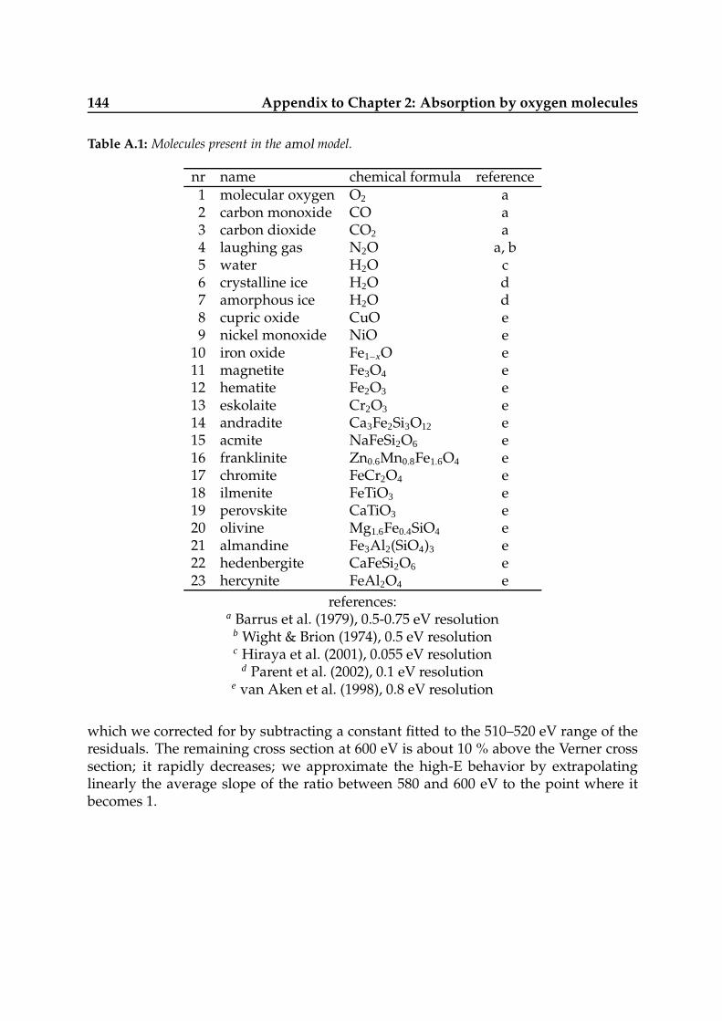
144 Appendix to Chapter 2: Absorption by oxygen molecules
Table A.1: Molecules present in the amol model.
nr name chemical formula reference1 molecular oxygen O2 a2 carbon monoxide CO a3 carbon dioxide CO2 a4 laughing gas N2O a, b5 water H2O c6 crystalline ice H2O d7 amorphous ice H2O d8 cupric oxide CuO e9 nickel monoxide NiO e
10 iron oxide Fe1−xO e11 magnetite Fe3O4 e12 hematite Fe2O3 e13 eskolaite Cr2O3 e14 andradite Ca3Fe2Si3O12 e15 acmite NaFeSi2O6 e16 franklinite Zn0.6Mn0.8Fe1.6O4 e17 chromite FeCr2O4 e18 ilmenite FeTiO3 e19 perovskite CaTiO3 e20 olivine Mg1.6Fe0.4SiO4 e21 almandine Fe3Al2(SiO4)3 e22 hedenbergite CaFeSi2O6 e23 hercynite FeAl2O4 e
references:a Barrus et al. (1979), 0.5-0.75 eV resolution
b Wight & Brion (1974), 0.5 eV resolutionc Hiraya et al. (2001), 0.055 eV resolution
d Parent et al. (2002), 0.1 eV resolutione van Aken et al. (1998), 0.8 eV resolution
which we corrected for by subtracting a constant fitted to the 510–520 eV range of theresiduals. The remaining cross section at 600 eV is about 10 % above the Verner crosssection; it rapidly decreases; we approximate the high-E behavior by extrapolatinglinearly the average slope of the ratio between 580 and 600 eV to the point where itbecomes 1.

References
Anders, E. & Grevesse, N. 1989, Geochim. Cosmochim. Acta, 53, 197Barrus, D. M., Blake, R. L., Burek, A. J., Chambers, K. C., & Pregenzer, A. L. 1979,
Phys. Rev. A, 20, 1045Bhattacharyya, S. & Strohmayer, T. E. 2007, ApJ, 664, L103Binney, J. & Merrifield, M. 1998, Galactic Astronomy, ed. Binney, J. & Merrifield, M.Blades, J. C. & Morton, D. C. 1983, MNRAS, 204, 317Blitz, L., Spergel, D. N., Teuben, P. J., Hartmann, D., & Burton, W. B. 1999, ApJ, 514, 818Caballero-Garcıa, M. D., Miller, J. M., Trigo, M. D., et al. 2009, ApJ, 692, 1339Chakravorty, S., Kembhavi, A. K., Elvis, M., & Ferland, G. 2009, MNRAS, 393, 83Chen, Y. Q., Zhao, G., Carrell, K., & Zhao, J. K. 2011, AJ, 142, 184Christian, D. J. & Swank, J. H. 1997, ApJS, 109, 177Collins, J. A., Shull, J. M., & Giroux, M. L. 2004, ApJ, 605, 216Costantini, E., Freyberg, M. J., & Predehl, P. 2005, A&A, 444, 187Costantini, E., Pinto, C., Kaastra, J. S., et al. 2012, A&A, 539, A32Cox, D. P. & Reynolds, R. J. 1987, ARA&A, 25, 303Dame, T. M., Hartmann, D., & Thaddeus, P. 2001, ApJ, 547, 792de Vries, C. P. & Costantini, E. 2009, A&A, 497, 393de Vries, C. P., den Herder, J. W., Kaastra, J. S., et al. 2003, A&A, 404, 959den Herder, J. W., Brinkman, A. C., Kahn, S. M., et al. 2001, A&A, 365, L7Detmers, R. G., Kaastra, J. S., Steenbrugge, K. C., et al. 2011, A&A, 534, A38, (paper III)Dickey, J. M. & Lockman, F. J. 1990, ARA&A, 28, 215Draine, B. T. 2011, Physics of the Interstellar and Intergalactic MediumDrake, J. J. & Testa, P. 2005, Nature, 436, 525Ebrero, J., Kriss, G. A., Kaastra, J. S., et al. 2011, A&A, 534, A40, (paper V)Esteban, C., Garcıa-Rojas, J., Peimbert, M., et al. 2005, ApJ, 618, L95Ferland, G. J. 2005, Hazy, A Brief Introduction to Cloudy 05.07, ed. Ferland, G. J.Ferland, G. J., Korista, K. T., Verner, D. A., et al. 1998, PASP, 110, 761Ferriere, K. M. 2001, Reviews of Modern Physics, 73, 1031Finkbeiner, D. P. 2003, ApJS, 146, 407Fox, A. J., Savage, B. D., & Wakker, B. P. 2006, ApJS, 165, 229
146 References
Freyberg, M. J. & Egger, R. 1999, in Highlights in X-ray Astronomy, ed. B. Aschenbach& M. J. Freyberg, 278
Friel, E. D., Janes, K. A., Tavarez, M., et al. 2002, AJ, 124, 2693Frisch, P. C. & Slavin, J. D. 2003, ApJ, 594, 844Galloway, D. K., Muno, M. P., Hartman, J. M., Psaltis, D., & Chakrabarty, D. 2008,
ApJS, 179, 360Ghavamian, P., Aloisi, A., Lennon, D., et al. 2009, Preliminary Characterization of the
Post- Launch Line Spread Function of COS, Tech. rep.Gnat, O. & Sternberg, A. 2007, ApJS, 168, 213Green, J. C., Froning, C. S., Osterman, S., et al. 2012, ApJ, 744, 60Greiner, J., Hasinger, G., & Kahabka, P. 1991, A&A, 246, L17Gummersbach, C. A., Kaufer, A., Schaefer, D. R., Szeifert, T., & Wolf, B. 1998, A&A,
338, 881Haardt, F. & Madau, P. 2001, in Clusters of Galaxies and the High Redshift Universe
Observed in X-rays, ed. D. M. Neumann & J. T. V. TranHaardt, F. & Madau, P. 2012, ApJ, 746, 125Hachisu, I. & Kato, M. 2009, ApJ, 694, L103Hagihara, T., Yamasaki, N. Y., Mitsuda, K., et al. 2011, PASJ, 63, 889Hartmann, H. W. & Heise, J. 1997, A&A, 322, 591Hartmann, J. 1904, ApJ, 19, 268Heger, A., Cumming, A., Galloway, D. K., & Woosley, S. E. 2007, ApJ, 671, L141Heise, J., van Teeseling, A., & Kahabka, P. 1994, A&A, 288, L45Helton, L. A., Woodward, C. E., Vanlandingham, K., & Schwarz, G. J. 2008, Central
Bureau Electronic Telegrams, 1379, 1Henze, M., Pietsch, W., Haberl, F., et al. 2010, A&A, 523, A89Henze, M., Pietsch, W., Haberl, F., et al. 2011, A&A, 533, A52Hiraya, A., Nobusada, K., Simon, M., et al. 2001, Phys. Rev. A, 63, 042705in’t Zand, J. J. M., Keek, L., Cumming, A., et al. 2009, A&A, 497, 469Iwamoto, K., Brachwitz, F., Nomoto, K., et al. 1999, ApJS, 125, 439Jenkins, E. B. 2009, ApJ, 700, 1299Jones, A. P. 2000, J. Geophys. Res., 105, 10257Juett, A. M. & Chakrabarty, D. 2003, ApJ, 599, 498Juett, A. M., Schulz, N. S., & Chakrabarty, D. 2004, ApJ, 612, 308Juett, A. M., Schulz, N. S., Chakrabarty, D., & Gorczyca, T. W. 2006, ApJ, 648, 1066Kaastra, J. S., de Vries, C. P., Costantini, E., & den Herder, J. W. A. 2009, A&A, 497, 291Kaastra, J. S., de Vries, C. P., Steenbrugge, K. C., et al. 2011a, A&A, 534, A37, (paper II)Kaastra, J. S., Mewe, R., & Nieuwenhuijzen, H. 1996, in UV and X-ray Spectroscopy of
Astrophysical and Laboratory Plasmas, ed. K. Yamashita & T. Watanabe, 411Kaastra, J. S., Paerels, F. B. S., Durret, F., Schindler, S., & Richter, P. 2008, Space Sci. Rev.,
134, 155Kaastra, J. S., Petrucci, P.-O., Cappi, M., et al. 2011b, A&A, 534, A36, (paper I)Kahabka, P. & van den Heuvel, E. P. J. 1997, ARA&A, 35, 69Kalberla, P. M. W., Burton, W. B., Hartmann, D., et al. 2005, A&A, 440, 775Kato, M. & Hachisu, I. 1989, ApJ, 346, 424Kim, S.-H. & Martin, P. G. 1996, ApJ, 462, 296
147
Konami, S., Sato, K., Matsushita, K., et al. 2009, PASJ, 61, 941Kovetz, A., Prialnik, D., & Shara, M. M. 1987, Ap&SS, 131, 419Kriss, G. A. 2011, Improved Medium Resolution Line Spread Functions for COS FUV
Spectra, Tech. rep.Kriss, G. A., Arav, N., Kaastra, J. S., et al. 2011, A&A, 534, A41, (paper VI)Kriss, G. A., Green, R. F., Brotherton, M., et al. 2000, ApJ, 538, L17Krolik, J. H., McKee, C. F., & Tarter, C. B. 1981, ApJ, 249, 422Lee, J. C. & Ravel, B. 2005, ApJ, 622, 970Lee, J. C., Xiang, J., Ravel, B., Kortright, J., & Flanagan, K. 2009, ApJ, 702, 970Lehner, N. & Howk, J. C. 2011, Science, 334, 955Liu, J., Wang, Q. D., Li, Z., & Peterson, J. R. 2010, MNRAS, 404, 1879Lodders, K. 2003, ApJ, 591, 1220Lodders, K. & Palme, H. 2009, Meteoritics and Planetary Science Supplement, 72, 5154Lynch, D. K., Russell, R. W., Rudy, R. J., Woodward, C. E., & Schwarz, G. J. 2008,
IAU Circ., 8935, 1Maciel, W. J. & Costa, R. D. D. 2009, in IAU Symposium, Vol. 254, IAU Symposium, ed.
J. Andersen, J. Bland-Hawthorn, & B. Nordstrom, 38PMaciel, W. J. & Quireza, C. 1999, A&A, 345, 629Madej, O. K., Jonker, P. G., Fabian, A. C., et al. 2010, MNRAS, 407, L11Malkin, Z. 2012, arXiv:1202.6128Mattsson, L. & Andersen, A. C. 2012, MNRAS, 423, 38McCammon, D. & Sanders, W. T. 1990a, ARA&A, 28, 657McCammon, D. & Sanders, W. T. 1990b, ARA&A, 28, 657McGee, R. X. & Newton, L. M. 1986, Proceedings of the Astronomical Society of Aus-
tralia, 6, 358Mcnally, P. A. 1929, PASP, 41, 351Miller, J. M., Raymond, J., Fabian, A. C., et al. 2004, ApJ, 601, 450Morrison, R. & McCammon, D. 1983, ApJ, 270, 119Morton, D. C. & Blades, J. C. 1986, MNRAS, 220, 927Munari, U., Siviero, A., Dallaporta, S., et al. 2011, New Astronomy, 16, 209Murphy, E. M., Lockman, F. J., Laor, A., & Elvis, M. 1996, ApJS, 105, 369Naik, S., Banerjee, D. P. K., & Ashok, N. M. 2009, MNRAS, 394, 1551Nakano, S., Beize, J., Jin, Z., et al. 2008, IAU Circ., 8934, 1Nauenberg, M. 1972, ApJ, 175, 417Ness, J.-U., Osborne, J. P., Dobrotka, A., et al. 2011, ApJ, 733, 70Netzer, H. 2008, New Astron. Rev., 52, 257Nieva, M.-F. & Przybilla, N. 2012, A&A, 539, A143Nomoto, K., Tominaga, N., Umeda, H., Kobayashi, C., & Maeda, K. 2006, Nuclear
Physics A, 777, 424Oegelman, H., Beuermann, K., & Krautter, J. 1984, ApJ, 287, L31Oegelman, H., Orio, M., Krautter, J., & Starrfield, S. 1993, Nature, 361, 331Orio, M., Covington, J., & Ogelman, H. 2001, A&A, 373, 542Paerels, F., Brinkman, A. C., van der Meer, R. L. J., et al. 2001, ApJ, 546, 338Page, K. L., Osborne, J. P., Evans, P. A., et al. 2010, MNRAS, 401, 121Parent, P., Laffon, C., Mangeney, C., Bournel, F., & Tronc, M. 2002, The Journal of Chem-

148 References
ical Physics, 117, 10842Patruno, A., Rea, N., Altamirano, D., et al. 2009, MNRAS, 396, L51Pedicelli, S., Bono, G., Lemasle, B., et al. 2009, A&A, 504, 81Petz, A., Hauschildt, P. H., Ness, J.-U., & Starrfield, S. 2005, A&A, 431, 321Pietsch, W., Fliri, J., Freyberg, M. J., et al. 2005, A&A, 442, 879Pinto, C., Kaastra, J. S., Costantini, E., & Verbunt, F. 2010, A&A, 521, A79Pinto, C., Kriss, G. A., Kaastra, J. S., et al. 2012a, A&A, 541, A147Pinto, C., Ness, J.-U., Verbunt, F., et al. 2012b, A&A, 543, A134Predehl, P. & Schmitt, J. H. M. M. 1995, A&A, 293, 889Provencal, J. L., Shipman, H. L., Koester, D., Wesemael, F., & Bergeron, P. 2002, ApJ,
568, 324Rauch, T. & Werner, K. 2010, Astronomische Nachrichten, 331, 146Richter, P. 2006, in Reviews in Modern Astronomy, Vol. 19, Reviews in Modern Astron-
omy, ed. S. Roeser, 31Rolleston, W. R. J., Smartt, S. J., Dufton, P. L., & Ryans, R. S. I. 2000, A&A, 363, 537Rudy, R. J., Lynch, D. K., Russell, R. W., Woodward, C. E., & Covey, K. 2008, IAUC,
8938, 2Savage, B. D., Sembach, K. R., Wakker, B. P., et al. 2003, ApJS, 146, 125Schattenburg, M. L. & Canizares, C. R. 1986, ApJ, 301, 759Schlegel, D. J., Finkbeiner, D. P., & Davis, M. 1998, ApJ, 500, 525Sembach, K. R., Savage, B. D., Lu, L., & Murphy, E. M. 1995, ApJ, 451, 616Sembach, K. R., Savage, B. D., Lu, L., & Murphy, E. M. 1999, ApJ, 515, 108Sembach, K. R., Wakker, B. P., Savage, B. D., et al. 2003, ApJS, 146, 165Shapiro, P. R. & Field, G. B. 1976, ApJ, 205, 762Shull, J. M., Jones, J. R., Danforth, C. W., & Collins, J. A. 2009, ApJ, 699, 754Simpson, J. P., Colgan, S. W. J., Rubin, R. H., Erickson, E. F., & Haas, M. R. 1995, ApJ,
444, 721Smith, N. & Owocki, S. P. 2006, ApJ, 645, L45Snowden, S. L., Egger, R., Finkbeiner, D. P., Freyberg, M. J., & Plucinsky, P. P. 1998,
ApJ, 493, 715Spitzer, Jr., L. 1956, ApJ, 124, 20Stasinska, G., Prantzos, N., Meynet, G., et al., eds. 2012, EAS Publications Series,
Vol. 53, Oxygen in the UniverseStruder, L., Briel, U., Dennerl, K., et al. 2001, A&A, 365, L18Takahashi, T., Mitsuda, K., Kelley, R., et al. 2010, in Society of Photo-Optical Instru-
mentation Engineers (SPIE) Conference Series, Vol. 7732Thompson, T. W. J., Galloway, D. K., Rothschild, R. E., & Homer, L. 2008, ApJ, 681, 506Trumper, J., Hasinger, G., Aschenbach, B., et al. 1991, Nature, 349, 579Trumpler, R. J. 1930, Lick Observatory Bulletin, 14, 154Ubertini, P., Bazzano, A., Cocchi, M., et al. 1999, ApJ, 514, L27van Aken, P. A., Liebscher, B., & Styrsa, V. J. 1998, Physics and Chemistry of Minerals,
25, 494Verner, D. A. & Yakovlev, D. G. 1995, A&AS, 109, 125Wakker, B. P. 2006, ApJS, 163, 282Wakker, B. P. & van Woerden, H. 1997, ARA&A, 35, 217
149
Wang, Q. D. 2009, in American Institute of Physics Conference Series, Vol. 1156, Amer-ican Institute of Physics Conference Series, ed. R. K. Smith, S. L. Snowden, &K. D. Kuntz, 257–267
Whittet, D. C. B. 2010, ApJ, 710, 1009Wight, G. & Brion, C. 1974, Journal of Electron Spectroscopy and Related Phenomena,
3, 191Williams, D. A. & Taylor, S. D. 1996, QJRAS, 37, 565Williamson, F. O., Sanders, W. T., Kraushaar, W. L., et al. 1974, ApJ, 193, L133Wilms, J., Allen, A., & McCray, R. 2000, ApJ, 542, 914Xiang, J., Zhang, S. N., & Yao, Y. 2005, ApJ, 628, 769Yamagata, T. & Yoshii, Y. 1994, in IAU Symposium, Vol. 161, Astronomy from Wide-
Field Imaging, ed. H. T. MacGillivray, 420Yao, Y., Schulz, N. S., Gu, M. F., Nowak, M. A., & Canizares, C. R. 2009a, ApJ, 696, 1418Yao, Y. & Wang, Q. D. 2005, ApJ, 624, 751Yao, Y. & Wang, Q. D. 2006, ApJ, 641, 930Yao, Y., Wang, Q. D., Hagihara, T., et al. 2009b, ApJ, 690, 143York, D. G. 1974, ApJ, 193, L127York, D. G., Songaila, A., Blades, J. C., et al. 1982, ApJ, 255, 467Zdziarski, A. A., Gierlinski, M., Mikołajewska, J., et al. 2004, MNRAS, 351, 791

150 References
Curriculum Vitae
I was born on 9th of April 1982 in Naples, Italy. I developed first interests in Astronomysince the last year of my primary school when I asked my father to buy me a smalltelescope to search for stars invisible to the naked eye. Later during the first schoollectures on the birth of the Solar system I completely devoted my self to stars and theirmysteries. Sunce then I already knew what would be my future.
After the scientific lyceum, I attended the University of Naples and obtained thedegree in physics. Here I followed interesting laboratories for the solar observation andspecialized in astrophysics in May 2008. At the Observatory of Capodimonte, Naples, Ifamiliarized with different kinds of telescopes and devices through which I developedmy observational skills. In Naples, I did my master degree research with GiuseppeLongo and Maurizio Paolillo focusing on the X-ray variability of active galactic nucleias probe of black hole masses and accretion of matter.
I started my PhD research at SRON in November 2008 working on X-ray spec-troscopy of the interstellar medium of our Galaxy with Frank Verbunt and Jelle Kaas-tra. I have traveled around the world and attended several interesting conferences thatimproved the quality of my work. Through the working visit at Jan-Uwe NEss (ESAC,Madrid, Spain) and Jerry Kriss (STScI, Baltimore, USA) I could work in rather differentresearch fields concerning nova ejecta and circumgalactic medium. I have also workedas tutor in the University of Utrecht in the courses of General Relativity (with PeterHoyng and John Heise) and Galaxies (with Dr. Soeren Larsen). This thesis summa-rizes the results of my PhD research obtained between November 2008 and October2012. I will spend the next two / three years as post doc at the Institute of Astronomyin University of Cambridge, UK, in the research group of Andy Fabian.

152 Curriculum Vitae
Acknowledgements
I was younger than 10 when me and my parents tried to understand why those littlepoints in the sky had different colors. We did not really know the reasons for sucha difference. This was just the beginning. My mother, Maria, subscribed me to themonthly journal “Video Astronomy” and as soon as I read about stars which cannotbe seen with the naked eye, I asked my father, Ettore, to buy me a small efficient tele-scope to search for “invisible stars” and special features on planets and moons. A littleamateur was just born. My interests in the Solar system were improved during thelectures at the intermediate and high school. Finally, I realized that stars have differentcolors due to their temperatures and chemistry, but how were the elements producedin the stars? How were they shared with the other stars in the Galaxy - this beauti-ful city hosting billions of different astronomical objects? These matters were part ofthe several interests which brought me to undergo physics studies and to specialize inastrophysics. It took me a while to understand that the more I learned, the wider theamount of question was. My eagerness in understanding the sky continuously grewup in these early 30 years of my life. I really hope that this trend will stand!
The development of this thesis was possible first of all because I reached SRON. Thishappened because my supervisors in Naples, Giuseppe Longo, Maurizio Paolillo, andBetty De Filippis, provided me the hints for carrying out a very interesting and up-to-date master thesis. Before them Massimo Capaccioli and Ester Piedipalumbo enabledme to write a bachelor thesis on the gravitational lensing phenomenon which turnedout to be very helpful during my teaching in the Utrecht University with great personslike Peter Hoyng, John Heise, and Soeren Larsen. This manuscript shows the work ofthese last four years in the Netherlands. The most beautiful period of my life withoutany doubt. I am very thankful to my advisors Frank Verbunt, Jelle Kaastra and ElisaCostantini who guided me to the production of a highly interesting work. They taughtme how to study scientific matters, to criticize results and to find solutions to differentkinds of problems. Thanks to them I am not anymore the little, afraid student thatcame here 4 years ago. I want also to thank Jan-Uwe Ness (ESAC, Spain) and JerryKriss (STScI, US) who helped me to carry out this work with new ideas and invitation

154 Acknowledgements
to visit them abroad. The LKBF (Leids Kerkhoven-Bosscha Fonds) provides me withthe funds necessary for deepening my research through several business trips.
These four years at SRON were really amazing thank to the people that surroundedme, especially in the beginning, such as Jacobo and Silvana, Rob, Ton, Manuel, Jelle dePlaa, Peter Jonker, Daniel, Lucien, Remco and Nynke, Wim, Jan-Willem, Jean, Estherand Marlies, Eva and Gio, Oliwia, Enya, Norbert, Peter den Hartog, Marianne, Chris,Pourja, Theo, Hiroki, and Artur. Many thanks also to Matthijs for the several amazingand useful discussions! Special thanks and hugs will be always reserved to my firstofficemate zen power Yan (and his wife Froukje), the only person able to handle withmy fancy and funny jokes 24/7. He has been the best colleague, a good friend, andthe living fun for me at SRON. I cannot imagine how would have been here withouthim. After he left, I luckily shared the office with Marianne, thanks to whom I stillhad a great time therein. Many thanks to all those colleagues that shared with me nicemoments during the SRON science days, the Sinterklaas nights, the social meetings atthe Utrecht University, and the work conferences I have attended.
These four “Dutch” years have been the most beautiful of my life thank to the manyfriends I made. I cannot name all, but the most important for me were Ariadne, Vi-tor, Chantal, Gerry, Andre, Claudia, Ken, Renata, Jesse, Louise, Simona, Nita, Ro-han, Rosa, Andrew, Ratna, Raffa, Rafael, Susha, Kyoko, Maarten and Cecille, Miguel,Sam, Emmy, Ivano, Davide, Edouard, Petteri, Rianna, Paulius, Giuseppe, Sheba, Paulo,Geza, Oluchi, Father Herman, Loraine, Thais, Rajani, Pawel, Brigitte, Sylvia, Eline, aswell as my overseas friend and colleague Pierluigi. It is worth to say that you all mademe a better person. Last but not least, I want to thank Peter Hoyng and my friendWendy for helping me translating the summary of this thesis into Nederlandse. Thankyou Peter for let it appearing suitable also for the public audience and still many thanksfor the nice lectures of General Relativity we gave together at the Utrecht University.Wendy, mijn zielsverwant, the good and female version of me, thank you very muchfor the Dutch summary and for being the special between my friends. The beautifultime spent with you in the last Dutch summer showed me that I can feel like home evenin a foreigner country. Thank you very much also for the many motivations providedme to complete my thesis and to continue my profession in UK. I will always keep youin my heart wherever we’ll be. Special thanks to Jelle de Plaa, the genius, for alwayshelping me to solve software issues and to prepare such a beautiful thesis cover!
Una parte dei ringraziamenti, in Italiano, va dedicata alla mia stupenda famiglia.Come gia detto, senza il supporto morale - e non solo - dei miei genitori, io non sareiarrivato certamente qui. Mi avete dato la forza ed il coraggio necessari per andareavanti nei miei studi e avete fatto di me un vero e proprio uomo. Sono svariate lepersone della mia famiglia che amo e che mi hanno sempre supportato azzerando ledistanze in questi quattro anni. Su tutti figurano i miei nonni, zii e cugini paterni,i miei suoceri e le mie sorelle Mara, Monica e Adele. Tuttavia, se per tutte questepersone riesco a trovare una maniera per essere riconoscente, credo che non troveromai parole sufficienti a ringraziare mia moglie, Valentina, la mia compagna di vita da10 anni a questa parte: un punto fermo nella mia esistenza, la pazienza e la forza graziealle quali sono riuscito a superare ogni sorta di difficolta. In tutti questi anni hai datoun senso alla mia vita e sei stata una compagna fedele e giudiziosa. Grazie amore mio.