the conductivity, dielectric constant, …

THE CONDUCTIVITY, DIELECTRIC CONSTANT, MAGNETORESISTIVITY, 1/f NOISE AND THERMOELECTRIC POWER IN PERCOLATING RANDOM GRAPHITE--HEXAGONAL BORON NITRIDE COMPOSITES

JUNJIE WU

A thesis submitted to the Faculty of Science, University of the Witwatersrand, Johannesburg, in partial fulfilment of the requirements for the degree of Doctor of Philosophy.

Johannesburg, January 1997

DECLARATION

I DECLARE THAT THIS THESIS IS MY OWN, UNAIDED WORK. IT IS BEING SUBMITTED FOR THE DEGREE OF DOCTOR OF PHILOSOPHY IN THE UNIVERSITY OF THE WITWATERSRAND, JOHANNESBURG. IT HAS NOT BEEN SUBMITTED BEFORE FOR ANY DEGREE OR EXAMINATION IN ANY OTHER UNIVERSITY

/

(SIGNATURE OF CANDIDATE)

i

ACKNOWLEDGMENTS

I would like to express my sincere thanks to my supervisor, Professor David S.

McLachlan, for providing support, guidance and encouragement. lowe special thanks

to Dr. A. Albers, not only for helpful discussions and suggestions, but also for his

assistance in set-up the data acquisition system and in writing the computer program

for the magnetoresistance and Hall coefficient measurements. I am particularly grate

ful to Professors M. J. R. Hoch and J. D. Comins for their constant support in the

Physics Department.

I wish to extend my thanks to many people who helped me to produce this thesis.

Mr. A. Voorvelt and Mr. C. J. Sandrock contributed to the design and construction

of electronic circuits and apparatus used in this project. The staff of the mechani

cal workshop in the Physics Department produced numerous pieces of experimental

apparatus. Professor L. Schoning assisted in the interpretation of the X-ray results,

obtained by Mrs. J. Salemi. Professor Harahan of the Electrical Engineering De

partment lent me the HP3562A signal analyzer that made the 1/ f noise experiments

possible. Professor M. H. Moys and Mr. M. Van Nierop of the Chemical Engineer

ing Department made the results of grain size distributions available. Professor D.

Chandler of the Mechanical Engineering Department assisted with the work on the

universal testing machine. Many of the figures in chapter three have benefitted from

the excellent artwork of R. Smith. Fellow students Mr. D. Dube and Mr. C. Chiteme

helped me to prepare the powder samples for some grain shape experiments on the

scanning electron microscope, and to correct grammar and punctuation.

Most of all, however, I wish to express my deep gratitude to my wife Sijia and

my daughter Tianshu. Without their indispensable support, tireless enthusiasm, and

great patience through the years of this project, none of the works presented in this

thesis would have been possible.

ii

ABSTRACT

Percolation phenomena involving the electrical conductivity, dielectric constant,

Hall coefficient, magnetoconductivity, relative magnetoresistivity, 1/ f noise and ther

moelectric power are investigated in graphite (G) and hexagonal boron-nitride (BN)

powder mixtures. Two kinds of systems are used in the experiments: highly com

pressed discs and parallelepipeds, cut from these discs, as well as 50%G-50%BN and

55%G-45%BN powder mixtures undergoing compression.

The measured DC conductivities follow the power-laws 0"( <p, 0) ex: (<p-<Pc)t ( <Pc)

and O"(<p, 0) ex: (<Pc-<Pti (<p < <Pc), and the low frequency (lOOHz & 1000Hz) dielectric

constant varies as c( <p, W ~ 0) ex: (<Pc - <P )-S( <P < <Pc), where <Pc is the percolation

threshold, t and s are the conductivity exponents, and s is the dielectric exponent.

Near the percolation threshold and at high frequencies, the AC conductivity varies

with frequency as 0"( <p, w) ex: WX and the AC dielectric constant varies as c( <p, w) ex: w-Y,

where the exponents x and y satisfy the scaling relation x + y = 1. The crossover

frequency We scales with DC conductivity as Wc ex: O"q( <p, 0) ( <Pc), while on the

insulating side, Wc ~ 1, resulting in q ~O for the three G-BN systems. The loss

tangent tan t5( <p, w) (<p < <Pc) is found to have a global minimum, in contrary to the

results of computer simulations.

The Hall constant could not be measured using existing instrumentation. The

measured magnetoconductivity and relative magnetoresistivity follow the power-laws

- 6. 0" ex: (<p - <Pc)3.08 and 6.R/ R ex: (<p - <Pc)O.28 respectively. These two exponents,

iii

3.08 and 0.28, are not in agreement with theory.

The 1/ f noise was measured for the conducting discs and parallelepipeds. The

normalized 1/ f noise power varies as Sv I V 2 ex RW with the exponents w = 1.47 and

1.72 for the disc and parallelepiped samples respectively. Furthermore, the normalized

noise power near the percolation threshold is, for the first time, observed to vary

inversely with the square-root of sample volume.

Based on the Milgrom-Shtrikman-Bergman-Levy (MSBL) formula, thermoelectric

power of a binary composite is shown to be a linear function of the Wiedeman

Franz ratio. A scaling scheme for the Wiedeman-Franz ratio for percolation systems

is proposed, which yields power-law behavior for the thermoelectric power. The

proposed power-laws for the thermoelectric power can be written as (Sm - Md ex

( <Pc and as (Sm - /~1d ex (<Pc - <p)-h2 for <p < <Pc, where Sm is

the thermoelectric power for the composites, Afl is a constant for a given percolation

system, and hI and h2 are the two critical exponents. The experimental thermoelectric

power data for the G-BN conducting parallelepipeds was fitted to the above power

law for <Pc. A least squares fit yielded the exponent hI = -1.13 and parameter

MI =9.511l V I I< respectively.

Contents

List of Figures

List of Tables

1 INTRODUCTION

2 THEORY 2.1 Introduction . 2.2 Geometric Percolation ............ . 2.3 Percolation in Binary Continuum Composites

2.3.1 Critical Volume Fraction ....... . 2.3.2 Electrical Conductivity and Dielectric Constant 2.3.3 GEM Equation ............ . 2.3.4 Hall Coefficient and Magnetoresistance . . . 2.3.5 1/ f (flicker) Noise ............. . 2.3.6 Thermoelectric Power (Seebeck Coefficient)

2.4 The Nonuniversality of Critical Exponents .....

3 APPARATUS AND EXPERIMENTAL METHODS 3.1 Sample Fabrication . . . . . . . . . . 3.2 Sample Characterization . . . . . . .

3.2.1 Porosity of the Disc Samples. 3.2.2 X-ray diffraction ...... . 3.2.3 Stress-Strain Tests ..... . 3.2.4 Grain Size Distribution and Shape

3.3 Measurements of the Conductivity and Dielectric Constant 3.3.1 Measurements on the Disc and Parallelepiped Samples 3.3.2 Measurements on the Powder Samples ..... . . .

3.4 Measurements of the Magnetoresistance and Hall Coefficient 3.5 1/ f Noise Measurements .......... . 3.6 Measurements of the Thermoelectric Power. 3.7 Data Fitting Technique. . . ........ .

1

3

6

7

13 13 14 21 23 26 31 32 34 37 40

43 43 47 47 49 52 57 63 63 65 70 75 77 80

2

4 THE ELECTRICAL CONDUCTIVITY, DIELECTRIC CONSTANT AND MAGNETORESISTANCE 82 4.1 Introduction............................ 82 4.2 The DC Conductivity and Low Frequency Dielectric Constant 83

4.2.1 Results.......... 84 4.2.2 Discussion........ 91

4.3 The Complex AC Conductivity 101 4.3.1 The Exponents x and y 101 4.3.2 The Crossover Frequency We and Exponent q . 121 4.3.3 The Loss Tangent tan 8 129

4.4 The Magnetoresistance 135 4.5 Summary . . . . . . . . . . . . 139

5 THEl/jNOISE 5.1 Introduction................. 5.2 Sv jV2 as a Function of Sample Resistance 5.3 Dependence of Sv /V2 on Sample Size. 5.4 Summary . . . . . . . . . . . . . . . .

6 THE THERMOELECTRIC POWER 6.1 Introduction............... 6.2 New Power-Laws for the Thermoelectric Power. 6.3 Experimental Results and Discussion 6.4 Summary . . . . . . . . . . . . . . . . . . . . .

141 141 143 154 158

160 160 161 165 171

7 SUMMARY, CONCLUSION AND PROPOSALS FOR FUTURE WORK 172

Bibliography 177

List of the Figures

Fig. 2.1 Percolation network on a 50 x50 square lattice

Fig. 2.2 Relationship between the percolation threshold <Pc and the ratio Ii/1m

Fig. 3.1 Resistance vs. time( days) for a disc sample

Fig. 3.2 Porosity vs. the volume fraction <p for the disc samples

Fig. 3.3 X-ray traces for the disc samples

3

Fig. 3.4 The X-ray diffraction data for G-BN powders as a function of pressure

Fig. 3.5 A typical stress-strain relationship, obtained during compression, as used

in the disc making process

Fig. 3.6a Bond strength tests for a compressed graphite bar

Fig. 3.6b Bond strength tests for a compressed 50%G-50%BN bar

Fig. 3.6c Bond strength tests for a compressed BN bar

Fig. 3.7a Grain size distribution for <p = 0.82 (pure G)

Fig. 3.7b Grain size distribution for <p = 0.00 (pure BN)

Fig. 3.7c Grain size distribution for <p = 0.153

Fig. 3.7d Grain size distribution for <p = 0.164

Fig. 3.8 Photographs of the grain in powders: (a) <p=0.158; (b) <p=0.41

Fig. 3.9 Schematic diagram of the system used to measure the complex AC

conductivity of the powders

4

Fig. 3.10 Schematic diagram of the system used to measure the magnetoresistance

and l! all coefficient

Fig. 3.11 Apparatus used to measure the thermoelectric power

Fig. 4.1 The axial a( <p, 0) against <Pc) on a log-log

scale for the disc samples

Fig. 4.2b The axial a( <p, 0) against (<Pc - <p) (<p < <Pc) on a log-log scale for the disc

samples

Fig. 4.2c The axial low-frequency dielectric constant c( <p, 0) against (<Pc - <p) on a

log-log scale, for the disc samples

Fig. 4.3 The axial a( <p, 0) against <P for the disc samples over the full range of <Pc)

Fig. 4.5b The axial and transverse a( <p, 0) against (<p - <Pc) on a log-log scale for

the powders (<p < <Pc)

Fig. 4.5c The axial and transverse low frequency dielectric constant against (<p

<Pc) on a log-log scale for powders (<p < <Pc)

Fig. 4.6a The axial a( <p, w) against frequency for the disc samples

Fig. 4.6b The axial a( <p, w) against frequency for the 50%G-50%BN powder sys-

tem

Fig. 4.6c The axial a( <p, w) against frequency for the 55%G-45%BN powder system

Fig. 4.7 a a( <p, w) / a( <p, 0) against w / Wc for the disc samples

Fig. 4.7b a(<p,w)/a(<p, O) against w/wc for the 50%G-50%BN powder system

Fig. 4.7c a(<p,w)/a(<p, 0) against w/wc for the 55%G-45%BN powder system

Fig. 4.8a c( <p, w) (<p < <Pc) against frequency for the disc samples

Fig. 4.8b c( <p, w) (<p < <Pc) against frequency for the 50%G-50%BN powder system

Fig. 4.8c c( <p, w) (<p < <Pc) against frequency for the 55%G-45%BN powder system

Fig. 4.9a w . c( <p, w) (<p < <Pc) against frequency for the disc samples

5

Fig. 4.9b W • c-( ¢;, w) (¢; < ¢;e) against frequency for the 50%G-50%BN powder

system

Fig. 4.9c W • c-( ¢;, w) (¢; < ¢;e) against frequency for the 55%G-45%BN powder

system

Fig. 4.10a We against 11( ¢;, 0) for the disc samples

Fig. 4.lOb We against 11( ¢;, 0) for the 50%G-50%BN powder system

Fig. 4.10c We against 11( ¢;, 0) for the 55%G-45%BN powder system

Fig. 4.11a [w· c-(¢;,w)]/I1(¢;,O) (¢;:S ¢;e) against frequency for the disc samples

Fig. 4.11b [w, c-(¢;,w)]/I1(¢;,O) (¢; < ¢;e) against frequency for the 50%G-50%BN

powder system

Fig. 4.11c [w, c-(¢;,w)]/I1(¢;,O) (¢; < ¢;e) against frequency for the 55%G-45%BN

powder system

Fig. 4.12a tan 8 against frequency for the disc samples near ¢;e

Fig. 4.12b tan 8 against frequency for the 50%G-50%BN powder system near ¢;e

Fig. 4.12c tan 8 against frequency for the 55%G-45%BN powder system near ¢;e

Fig. 4.13 [11(H = 0) - I1(H = 1.5T)] against (¢; - ¢;e) on a log-log scale

Fig. 4.14 6R/ R against (</> - ¢;e) on a log-log scale

Fig. 5.1a Sv /V2 against frequency in the axial direction

Fig. 5.1 b Sv /V 2 against frequency in the transverse direction

Fig. 5.2a Sv against DC current in the axial direction

Fig. 5.2b Sv against DC current in the transverse direction

Fig. 5.3 Sv /V 2 against the sample resistance

Fig. 5.4 Sv /V 2 against the sample volume

Fig. 6.1 Sm against ¢; for the G-BN parallelepipeds

Fig. 6.2a Sm against ¢; for the AI-Ge films, showing the theoretical curve obtained

using a fixed ¢;e of 0.56

Fig. 6.2b Sm against ¢; for the Al - Ge films, showing the theoretical curves ob

tained using ¢;e as a fitting parameter

List of the Tables

Table 2.1 The percolation thresholds for a variety of lattices

Table 4.1 The <Pc, t, 5, and s for the G-BN systems

Table 4.2 The measured and calculated crossover frequency Wc

Table 5.1 The measured exponents I and {)

6

7

Chapter 1

INTRODUCTION

Percolation theory deals with both macroscopically and microscopically disordered

systems. The origin of percolation theory is attributed to Broadbent and Hammersley

(1957), who introduced lattice models for the flow of a fluid through a static random

medium, and showed, using geometrical and probabilistic concepts, that no fluid will

flow if the concentration of active medium is smaller than some nonzero threshold

value - a percolation threshold. Since the 70s, percolation models have involved the

concepts of scaling, which emphasizes particularly the so-called critical phenomena.

Percolation theory has become one of few theoretical techniques that is available to

describe strongly disordered materials.

Percolation theory is marked by the fact that it provides a well-defined, simple,

and intuitively satisfying model for granular binary composites, in which the rele

vant physical properties of the individual components differ widely. To be specific,

consider compacted random binary mixtures of conducting (metallic) and insulating

(dielectric) components, for which only an average grain size and overall composition

are known. Then, if the concentration of dielectric is not too large, electrons can

move through the sample via an "infinite" metallic cluster, resulting in conducting

sample. As the dielectric concentration increases the infinite metallic cluster becomes

less dense, and eventually breaks into isolated clusters embedded in dielectric ma

trix, resulting in insulating sample. Denoting the volume fraction of the conducting

8

component in the sample by <p, percolation theory predicts that there is a critical

value fract,ion <Pc, called a percolatiofL threshold, at which t,n infinite metallic cluster

spanning whole sample first appears, and the system undergoes a percolative metal

insulator transition (MIT). This percolation transition is the most fundamental and

striking feature of the percolation model, and makes percolation a natural model for

describing a diversity of physical processes.

In many aspects, the percolation transition is an analogue of second order phase

transition in thermodynamic systems. Near the percolation threshold, the percolation

quantity Q follows a power-law given by

(1.1 )

where a is a critical exponent characterizing the asymptotic behavior of Q as <Pc is

approached from below or above. Scaling laws relate the different exponents which

occur in a given percolation system, which means that the critical exponents appeared

in a percolation system are not independent of each other. The exponent a can be

positive or negative depending on what physical property is under study in the per

colation system. The values of a, found from computer simulations, are dependent

only on the dimensionality of system [Stauffer and Aharony 1994]. Exponents of this

nature are described as universal. Recent experimental and theoretical results show

that, in three dimensional continuum systems, the values of the same exponent could

differ considerably from system to system[Carmona et al. 1984, Kogut and Straley

1979, Feng et al. 1987, Balberg 1987a, and Nan 1993 and references therein]. It has

been shown that the particle size distribution, shape and orientation can influence

the percolation threshold <Pc [Kusy 1977, Balberg 1987b, and Dovzhenko and Zhirkov

1995] . Note that the power-law (1.1) is expected to hold only close to the percolation

threshold and then only if the investigated physical properties of the two components

are drastically different. If it is not the case, a variety of effective-medium theories

can be employed to model the properties of the composites.

9

The electrical transportation properties which have been studied experimentally

on continuum percolation systems include: electrical conducti lity, dielectric con

stant, 1/ f noise, Hall constant, magneto conductivity, and thermoelectric power (

thermopower). In addition the critical current density and critical field have also

been investigated, using a percolation approach, for inhomogeneous superconductors

[Deutscher and Rappaport 1979; Grave, Deutscher and Alexander 1982]. For perco

lation systems, the electrical conductivity and the dielectric constant are the most

extensively studied quantities. Some of the continuum percolation systems that have

been previously investigated include: amorphous carbon-teflon composites [ Song et

al. 1986], carbon-epoxy composites [McLachlan et al. 1990, Lee et al. 1993], nickel

polypropylene composites [Chen and Johnson 1991], carbon-wax mixtures [Chen and

Chou 1985; Chou and Jaw 1988; Chakrabarty et al. 1993], carbon-polymer composites

[Michels et al. 1989], carbon-PVC composites [Balberg and Bozowski 1982]' polyethy

lene gels-conducting polymer system [Fizazi et al. 1990], carbon fibers-polymer com

posites [Carmona et al. 1984], Ag-KCI composites [Grannan et al. 1981], glass-iron

balls mixtures [Benguigui 1985], plain and silver-coated glass microbead mixtures

[Laugier 1982, Laugier et al. 1986], glass-In mixtures [Lee et al. 1986], PrBa2Cu307-

Ag composites [Lin 1991], sintered silver beams [Deptuck et al. 1985], thin gold films

[Laibowitz and Gefen 1984; Hundley and Zettl 1988], granular Sn-Ar films [Rohde

and Micklitz 1989], thick bismuth ruthenate films [Nitsch et al. 1990], thick glass

Ru02 films [Pike 1978], and microemulsions [Van Dijk 1985, Van Dijk et al. 1986,

Moha-Ouchane et al. 1987, Peyrelasse et al. 1988, and Clarkson and Smedley 1988].

The Hall constants of only two percolation systems has been studied: AI-Ge films

[Dai et al. 1987] and Sn-Ar films [Rohde and Micklitz 1989]. The latter reference also

reported the investigation of the magnetoconductivity and relative magnetoresistivity.

The 1/ f noise is a sensitive probe of the microstructure of the infinite clusters

in percolation systems [Rammal, Tannous and Tremblay 1985]. Percolation systems,

in which 1/ f noise has been investigated, include: carbon-wax mixtures [Chen and

Chou 1985], copper particle-polymer composites [Pierre et al. 1990], Ah03-Pt cer-

10

mets [Mantese and Webb 1985 and Mantese et a1. 1986], thin gold films [Williams

and Budett 1969 and Koch et al. 1985], silver films [Octavio et a1. 1987], thin AI,

In, and Cr foils [Garfunkel and Weissman 1985], and AgPt-TFE mixtures [Rudman

et a1. 1986].

The percolation behavior of the thermoelectric power in AI-Ge films was investi

gated by Hurvits et a1. (1993).

The experimental results obtained from the above-mentioned continuum percola

tion systems have verified many aspects of percolation theory and provide a significant

experimental data for the application of percolation models. However, some discrep

ancies between theory and experiment still exist, and, therefore more experiments

are necessary to further advance the development of theoretical models, especially for

non universal exponents.

It should be noted that in most previous studies of a single continuum percola

tion system only one or two of the physical percolation properties were measured,

discussed, and compared with other experimental results and theoretical predictions.

In many cases, other percolation phenomena could have been measured on the same

system. This situation makes it difficult to compare and correlate the different expo

nents that have been obtained from experiments done on various percolation systems.

It should also be noted that for the Hall coefficient, magnetoresistivity and thermo

electric power only one or two previous sets of experimental data are available.

The primary objective of the study presented in this thesis is to observe as many

of these percolation phenomena as possible in a single reliable continuum percolation

system. The measured critical exponents and percolation thresholds are then used

to, where possible, test various theoretical models and the exponents are compared

with those obtained from other previous experiments. This full spectra of critical

exponents, all from the same system, should help to provide a more complete under

standing of percolation theory.

11

Various mixtures of graphite (G) and hexagonal boron-nitride (BN) powders, un

dergoing compression in the appropriate cell, compacted discs and the parallelepipeds

cut from these discs, were chosen as the subject of this study. In these systems the

graphite powder is the conducting component, while the hexagonal boron-nitride is

the insulating component. The reasons for choosing these systems are as follows.

Firstly, the insulating and conducting components have a very small conductivity

ratio ~ lxl0-17. Secondly, they have the same densities, 2.25g/cm3

, and nearly the

same unit hexagonal cell dimensions at room temperature: a = b = 2.464A and

c = 6.736A for graphite, while a = b = 2.504A and c = 6.661A for hexagonal boron

nitride [Lide 1994] . These properties made the two components indistinguishable

by the usual X-ray methods and easy to mix together to form random composites.

Thirdly, single crystals of G and BN show very similar stress-strain relationships along

either the c-axis or the a-b layer planar [Lynch and Drickamer 1966]. These properties

of two components appear to make the G-BN powder mixtures nearly ideal percola

tion systems, on which the critical volume fractions and many of the exponents that

appear in the percolation equations can be measured.

No previous investigation on the G-BN percolation systems has been reported in

the literature. Phenomena studied at room temperature include the DC conductivity,

AC conductivity and dielectric constant, magnetoconductivity or relative magnet ore

sistivity, 1/ f noise and thermoelectric power. It was not possible to measure the Hall

coefficient at room temperature or at liquid nitrogen temperature.

In Chapter two the various theoretical percolation equations, relevant to the mea

surements made on the G-BN percolation systems, are presented. The topics include

the geometric phase transition, where the basic concepts and elementary results are

introduced, the percolation equations for the various electrical transportation prop

erties, 1/ f noise and thermoelectric power for a binary continuum medium, as well

as recent progresses in the understanding of the nonuniversality of the critical expo

nents. Chapter three describes the experimental techniques and apparatus used in

this study. The results for the disc porosity, grain orientation, grain size distribution,

12

and the comparative strength of the interparticle bonds are given here. The various

powder cells employed for measuring the DC and AC conductivities and dielectric

constant in the axial (along the direction of compression) and transverse (perpendic

ular to the direction of compression) directions for SO%G-SO%BN and SS%G-4S%BN

powders and powder pouring methods are described in detail. The principles of

measurement, schematic diagrams and electrical circuits are given for the apparatus

and techniques used to measure the electrical conductivity, dielectric constant, Hall

constant, magnetoconductivity, 1/ f noise and thermoelectric power. Chapter four

presents the experimental results of the electrical conductivity, dielectric constant

and magnetoconductivity. Chapter five presents the experimental 1/ f noise results

obtained from the compressed conducting disc and parallelepiped samples near the

percolation threshold. In Chapter six, power-laws to describe the Wiedeman-Franz

ratio in continuum percolation systems are proposed, which in turn lead to new

power-laws for the thermoelectric power near the percolation threshold. Measured

thermoelectric power data for the G-BN parallelepipeds, on the conducting side of

percolation threshold, is presented and fitted using one of the new power-laws for

the thermoelectric power, developed in this chapter. In all cases, the experimental

results are illustrated using a large number of graphs, while the observed or fitted

parameters, obtained from various theoretical expressions, namely the critical volume

fractions and exponents, are given in tables or the text where appropriate. Where

possible, comparisons between the present experimental results and those obtained

from other continuum percolation systems are made. Chapter seven of the thesis

summarizes and discusses the main results, and makes several suggestions for the

further investigations.

In order to look for signs of weak localization near percolation threshold, the tem

perature dependences of the resistances were studied using conducting G-BN paral

lelepipeds at temperatures from 1.8K to 300K, using a DIP system [Albers 1994].

Some of these samples, which had ¢> values very near the percolation threshold, were

also measured at temperatures from 1.4K to 30K and in magnetic fields up to 8.ST.

Since these experimental results were inconclusive, they are not included in this thesis.

13

Chapter 2

THEORY

2.1 Introduction

This chapter deals with the percolation theory of a number of phenomena in het

erogeneous conductor-insulator composites. A fairly complete overview of the theo

retical developments in this field is given. Some relevant numerical and experimental

results will also be discussed in this section, but only when it is necessary to prove or

to supplement the line of the theoretical arguments.

Since the 70s, percolation theory and its applications have been the subject of a

large number of review articles and some books. Some of the review articles quoted

here in chronological order are by Kirkpatrick (1973), Essam(1980), Deutscher et al.

(Ed., 1983), Clerc et al. (1990), Bergman and Stroud(1992), and Nan (1993). Stauffer

and Aharony's revised textbook (1994) provides the most recent complete review of

geometrical aspects of the percolation problem, with emphasis on cluster statistics,

renormalization group techniques, and numerical algorithms.

This chapter is organized as follows. Section 2.2 contains a detailed presentation

of the geometrical percolation problem, with emphasis on the critical exponents and

scaling laws. Section 2.3 presents the application of percolation theory to the mea

surements of various physical quantities measured in this thesis, and again emphasizes

14

the critical volume fraction and the existence of scaling laws. The microstructures

leading to differen~ ¢>cs are presented first. The percohtion equations, describing the

electrical conductivity, dielectric constant, magnetoresistance, Hall coefficient, 1/ f noise, and thermoelectric power, are then discussed. In addition, the GEM equation,

which interpolates between the two percolation equations, is discussed in this section.

The chapter ends with Section 2.4, in which the current models accounting for the

nonuniversality of the conductivity exponent are reviewed.

2.2 Geometric Percolation

The geometric phase transition can be studied, either as a bond or as a site per

colation problem. The bond percolation problem may always be converted into its

dual site percolation problem [Fisher, 1961]. The converse is however not true: not

every site percolation problem corresponds to a bond percolation problem. For this

reason, the site process is considered to be more fundamental. In this section, the ba

sic concepts and elementary results of geometric percolation are illustrated using the

site percolation model, which is also the most appropriate one for continuum systems.

A site percolation system, using a 50 x 50 square lattice, is shown in Fig. 2.1.

Each site is occupied (black squares) at random with probability P or empty (white

squares) with the complementary probability (l-p). The neighboring squares are

called nearest neighbours if they have one side in common but not if they touch

only at one corner. A group of occupied squares, connected through nearest neigh

bours, is called a cluster. A s-site cluster is a cluster containing s sites. When P is

small, most occupied squares are isolated or form very small clusters. The occupied

squares become more interconnected and form larger clusters as p is increased. At

percolation threshold Pc, an infinite cluster spanning the entire lattice appears.

For all p < Pc, there is no infinite cluster, and for p > Pc the infinite cluster co-exists

with smaller finite clusters, which join the infinite one as p is further increased.

(a) p = 0.1

(b) p = 0.3 :::::-.:: I a::. :-.:'::: •• :':'.::: :.:.: •••• . ........ .. ..... ... . ......... . .. ........... ..... ...............• .. ....... . . . .............. ...... . ......... .

'I .: •••• :':"::.::':'" ::.::~::- :::::.:'.:.:

I' .............. _..... . ................ .

I ..... ... . .......... . ............... . · .................................... . · ... .. ... ... ... ... . ............. . · .. ......... ...... .... ... ........ .. ... . ............. .. .. .. ... . .. . I:::', • ':- :':. I::: ••• : •• : •• ::': :: : ::: I:. ... ... .. . ........................... . ..... .... . ........ . ....... . ....... . .. ... .... ............ . ............. . .... ...... . . .... ........ ... ......... . II' ........ -........ ....... . ........ .

::1::' •• :':': .: ••••• :: : •• :: ••••• : • :.:" · ........................ _......... . ..... . ... .... ...... ........ . ..... . ......... . · ........ .... ....... . ......... . ..... . . ..... ..... .. ............ . ....... . · ............ ... .......... ........ ., ..... ...... ....... ..... ........ . .... . ... ....... ..... ... . ................. . 'i' . .... ... ... ...... ... ... . .. • '1 .. :.:::::.": -:.:':::'::'::.:':. :::::::.'. .... . ..... ....... ............. . ... . ::1. '::::.:: :::::::.:::::::. ::.' ::::::::::::. 'E: I •••••• •• •• ••• • • •• • ••••••••••••• •• . . . . ..... ...... .... . .. . . :: ..... ::: .. :: :' .. ::'.:::': ':::":' .. ::.:::.: I" II':.:':. :: : •••• '::.:' •• ::::::: : ••••• ::: • • :1":.:: •• '.:::.:':.:.:'::::. :.: :.: •••• '::.':: I ••• •• •••••••• •• •.•• •••• • ••••••••

I ····· . ....... ........ .. . .. . · .......... ..... ...... ........... ... .. ..... . .... .. ..... ...... .... . .. . · ... ........... ..... ... ... . ........ . . .. ..... .......... . ............. .

(c) p=0.6 .... . .... . . .. . ... : ... " '.. .. :':.' ........ :: ... .

I •••• • •••••• -::c' .. -.. : .: .::"': . :: .. :-.. '.: .:::: . ".: .:: ... ~:': ::::. : . : •••••• y: ••••.••• ::" •••••• :.. : ••••••

~;~::.:::;:: :~:. :;:i::~} ~; .. : ::;~;::;~~::r ::' : .. : ..... :.:: :: ':.:'.: ': '. .... .': . . ... ........ . ...... . · ... . . .... . .. :': .. : . - : .. :::: .. :.. : .:.::: :.: .::-. . : ...... :: ......... :: .. :: .. . · .. .. .... .... ...... . : '. :.: ::: ::: ;:::;:::~~~:. '. : .... :: .::: :: .. .... . ::.. .: .... :: .. ':: .:.' .. :.. . .:. ': .. ' .. : .. :.. . ....... : .•.•. : .... : · :' ::: .. - .::. '::.: :',:: : .::::' . '.' ::;: ;:;=:.';: .:;:.' ':;':.'. ::::.:: .. ' .::.:. '.: .'::.:: : .. :'::.:.: : .. : .. ': :::.: .... : (d) • Pl"rl·tllalin~ dusler .................... . ................... . ....................... .. . ................ . ..•. :.: ...• :.:.:.:.:.:.:.:.:.:.:.: .•.• :.:.:...... . ................. . ::::::::::::::::::.: ::: r:: .:.:::.~~.~:;E.E.E.E.E.:.:.EE.:.:E.:.: ...... ......... . ........ ........ . .... . .......... . ..... ..... ... . .. :.... . ......... . ~~~~:.:::~::~~~;~~;~~~m;·:... ::~~~~~~~~~~ .. ::: · . ...... ......... ... . ... . . · . ........... . .. . · .:.. . ... :::::::::.: ........ : . '.';:: .. . :':::: .;.' : "::::.: ':.' . ~. : .:: '.' .:: .. .. .... .. . ..... " . . ....... .. . .. ... .... . . .. '.' ::.:.:: •..... : .•.. :.: ...... .. :. .: :m:m~~:::mg:. , .... : .;;;'~;: :.~:: .... . ................... .. ... . .. · ..................... .... . .. :.. ':::::::::::::::::::.. . ... : .. :::::::: .. : ............ _........... . .....•..........

::::::::::::::::::::::::' : ... ::::::::::::::: .. . .......... _........ . ............... . . .................• . ............... . .... . .................... . ............ . · ........................................... . :. . :::::::::::::::::::::::.:::::::::::::::: .. , .......... _ .................. _ ......... .

15

Fig. 2.1 Percolation network on a 50 x 50 square lattice for three values of P is shown in the figures. Occupied and empty sites are represented by black and white squares, respectively. The 'infinite' (percolating) cluster near the percolation threshold Pc =0.59 is also shown. The arrow indicates that (d) is obtained from (c) by deleting all clusters except for the percolating one. (Reproduced from Smilauer 1991)

16

The geometric phase transition from isolated clusters to an infinite cluster, plus

small isolated ones, is r:alled the percolation transition. The percolation threshold Pc

is a critical point, such as occur in second-order phase transitions in thermodynamic

systems, at which many properties of a percolation system change dramatically, as

a consequence of the appearance of the infinite cluster. The percolation threshold is

the key to understand the percolation phenomena of many physical systems. Table

2.1 shows the Pc values known either exactly (in one and two dimensions) or from

numerical work (in three or higher dimensions). It is evident from this table that

the value of the percolation threshold Pc varies with the type of lattice and with the

dimensionality of lattice. In two dimensions, the pc values extend from 0.35 to 0.70;

in three dimensions, pc spans the range from 0.12 to 0.43 for regular crystal lattices.

The volume fraction, <p, is defined as

<P = vp, (2.1 )

where v is the filling factor of the lattice. The volume fraction <P is, in general, the

fraction of space that is taken up by the occupied sites. The two dimensional case

is shown in Fig. 2.1, where the volume fraction is the ratio of shaded area to that

of the whole lattice area. The critical volume fraction <Pc is defined as the value of <P

at the percolation threshold, that is, <Pc = VPc. Scher and Zallen (1970) pointed out

that <Pc, in contrast to Pc, is remarkably insensitive to lattice structures with the same

dimensionality. This is seen by comparing the fourth and eighth columns of Table

2.1. To within a few percent, the critical area or volume fraction for site percolation

is 0.45 in two dimensions and 0.16 in three dimensions. The approximate dimensional

invariance of the critical volume fraction <Pc suggests that <Pc is a more fundamental

quantity than Pc, in site lattice percolation problems. For this reason, Pc is used only

to present lattice percolation models, while <Pc will be used in all future discussions

on continuum percolation systems, both theoretical and experimental.

In addition to the percolation threshold Pc or critical volume fraction <Pc, six

other basic quantities or concepts are used to describe the geometrical properties and

Table 2.1 The bond (p~ond) and site (p~ite) percolation thresholds on a variety of lattices (after Zallen 1983).

Dimension- Filling ali~ Lattice or Coordination Factor

d Stnu:ture Pcbond p/" z v

Chain 2

2 Triangular 0.3473 0.5000 6 0.9069 2 Square 0.5000 0.593 4 0.7854 2 Kagome 0.45 0.6527 4 0.6802 2 Honeycomb 0.6527 0.698 3 0.6046

3 fcc 0.119 0.198 12 0.7405 3 bee 0.179 0.245 8 0.6802 3 sc 0.247 0.311 6 0.5236 3 Diamond 0.388 0.428 4 0.3401

4- sc 0.160 0.197 8 0.3084 4- fcc 0.098 24 0.6169

5 sc 0.118 0.141 10 0.1645 5 fcc 0.054 40 0.4653

6 sc 0.094 0.107 12 0.0807

zPcbond "Pc"" ill cPc

2

2.08 0.45 2.00 0.47 1.80 0.44 1.96 0.42

2.0 ± 0.2 0.45 ± 0.03

1.43 0.147 1.43 0.167 t.48 0.163 1.55 0.146

1.5 ± 0.1 0.16 ± 0.02

1.3 0.061 0.060

1.2 0.023 0.025

1.1 0.009

~

~

18

statistics of clusters in a percolation lattice [Stauffer and Aharony 1994, and refer

ences therein]. These additional concepts are: the corrdation length, cluster size,

order parameter, density-density correlation function, scaling law and universality,

and fractal structures. Before discussing these six concepts, the distribution function

of cluster size should be introduced.

The cluster number ns is defined as the density of finite clusters, consisting of

s occupied and connected sites. It is nothing but the number of such clusters per

unit volume in the thermodynamic limit [Clerc et al. 1990]. Near the percolation

threshold Pc, the distribution of cluster numbers is assumed to follow the scaling form

(2.2)

where z = Ip - Pc Is"", ( and T/ are both critical indices, and f( z) is a universal scaling

function, where f(O) = 1. Equation (2.2) is fundamental in the scaling theory of

percolation phenomena, as will be seen below. Consider the k-th moment of the site

number s in a cluster, which is given by Ls sk ns . For P near Pc, the singular part of

this k-th moment can be calculated by replacing the sum with an integration. This

replacement is valid since only large clusters are responsible for singularity. Direct

calculation [Stauffer and Aharony 1994] yields

= qo Ip _ Pc I (<;-l-k)/.,., t;o Izl(1+k-<;)/.,., Z-l f(z)dz, T/ Jo (2.3)

Evaluation of the integral on the right-hand side of the above equation gives

L .'/ns ex: Ip - Pc I (<;-l-k)/.,., . (2.4) s

(1) The correlation length e

19

Mathematical calculations show that the correlation length measures the mean

distance between tWI) sites belonging to the same clusterl which contributes to the

divergences of the k-th moment of the site number. As the percolation threshold is

approached, large clusters join, becoming larger and larger, and the correlation length

diverges according to the power-law

(2.5)

where v is a constant. ~ is measured in units of the site length ao, implying that the

correlation length is actually ao~. Computer simulations [See Table I of Harris 1983]

yield v=1.35 and 0.88 in two and three dimensions respectively.

(2) The cluster size

The number of sites within the largest cluster near pc is s(, which diverges as

1 1-1/11

s( ex P - Pc . (2.6)

The average size sav.of the clusters near Pc, derived from Equation (2.4), is

2:s sns 1 1 'Y Sav. = ex p - Pc - , 2:s ns

(2.7)

where I is an exponent.

(3) The order parameter P 00

P 00 is defined as the probability that any occupied site, chosen at random, belongs

to the infinite cluster. At p < Pc there is no infinite cluster and Poo = 0; at p = 1,

all sites are connected together, therefore Poo = 1. In general Ex> can be expressed,

according to its definition, as

1 Poo=l--~sns.

p s

Near the percolation threshold pc, P 00 follows the power-law

(2.8)

(2.9)

20

(4) The density-density correlation function g(l)

This function g(1) gives the probability for two occupied sites separated by distance

1 to belong to the same cluster, and can be written as

9(1) = ~-~ F(l/O, (2.10)

where F(u) denotes a scaling function with F(u« 1)", u-(i/I/ and F(u» 1)~1.

(5) The scaling laws and universality

The exponents in Equations (2.5) to (2.9) are called critical exponents in the

study of percolation phenomena. From (2.4) it is clear that these exponents are not

independent of each other. Comparing (2.4) with (2.5) - (2.9), one obtains the

following scaling laws

2 - a = (~ - 1) /ri, (3 = (c; - 2) /7J, -, = (c; - 3) /7J, (2.11)

and

2 - a = , + 2(3, lid = (3 + l/ri, (2.12)

where d is the Euclidean spatial dimensionality of the lattice. From these scaling laws

it can be shown that only two of these exponents are independent. Universality in

the percolation transition requires that these exponents depend only on the lattice

dimensionality, and not on the local structure of the lattices. The scaling laws and

universality provide one of the most compelling arguments to apply lattice percola

tion theory to continuum percolation systems, to test whether these concepts hold

for continuum systems

(6) The fractal structure

The geometry of the percolation cluster near <Pc is described by irregular geometric

fractals, or statistically self-similar fractals, within the length scale L such that ao < <

21

L < < ~. For L > > ~, the percolation cluster appears homogeneous and the detailed

structure of the percolation network is unimportant in determining the network's

physical properties. Combining equations (2.5) and (2.7), one obtains

(2.13)

where the exponent dj is the fractal dimension of the percolation cluster. The scal

ing laws relate the fractal dimension dj to other critical exponents and the lattice

dimensionality d (d < 6) as

dj = d - (3/v. (2.14)

This fractal dimension d j is found to be 1. 9 in two dimensions and about 2.5 in

three dimensions [Stauffer and Aharony 1994]. Since (3/v>O, the finite clusters at the

percolation threshold are fractals such that their fractal dimension d j is smaller than

their lattice dimension d.

2.3 Percolation in Binary Continuum Composites

A binary continuum percolation system is a topologically disordered mixture

of two components with drastically different physical properties, e.g. conductor

insulator, conductor-superconductor, and sol-gel. In this section, only conductor

insulator composites will be discussed, as this is the subject of the thesis. Conductor

insulator composites consist of a conductor, with conductivity (7c, and an insulator,

with conductivity (7i and dielectric constant Ci, such that (7i/ (7c < < 1. The con

ducting volume fraction <P is defined, by analogy to the site lattice problem, as the

fraction of the volume taken up by the conducting component. Such systems undergo

a metal-insulator transition at a critical conducting volume fraction <Pc, at which the

conducting component first forms a continuously connected infinite cluster through

the sample. In this infinite cluster, the current is carried only by the backbone, which

is obtained from the infinite cluster by removing all the dead or "dangling" ends,

22

which do not participate in the conduction.

The underlying concept of topological disorder is important in distinguishing con

tinuum percolation systems from the lattice problem. II). lattice percolation, the

structural starting point is that of a regular geometrical object-a periodic lattice.

Disorder is introduced by superimposing on the sites or bonds of such a lattice, a ran

domly assigned two-state property (empty/occupied). The bimodal statistical vari

able, imposed on a regular geometrical structure, gives rise to a stochastic-geometry

situation [Frisch and Hammersly, 1963]. The situation in the continuum system, how

ever, represents a higher order of stochastic geometry, because the disorder-generating

statistical variable (conductor/insulator) is superimposed on a structure that is itself

topologically disordered.

The universality and scaling laws discussed in the previous section suggest that

one may apply lattice results to continuum percolation systems. Recent developments

in understanding the continuum system have revealed many special features of such

systems, that make this branch of percolation studies attractive and practical in its

own right. One of these aspects, the nonuniversality of critical exponents, or so called

"continuum correction", will be discussed in Section 2.4.

Scaling theory predicts that many physical properties of percolation systems will

scale with the conducting volume fraction <P as a power-law with the form I<p - <PcI C\

where the critical exponent a can be positive or negative depending upon the prop

erty being studied, and <Pc is the critical conducting volume fraction. The critical

exponents used in this thesis are:

l/, correlation length exponent

t, DC conductivity exponent on the conducting side

s, DC conductivity exponent on the insulating side

s, dielectric constant exponent

'" and w, 1/ f noise exponents

g, Hall coefficient exponent

t m , ma,gnetoconductiv'ity exponent

hI, thermoelectric exponent on the conducting side

h2' thermoelectric exponent on the insulating side

23

The following subsections will discuss the critical volume fraction and the various

percolation equations, which will be used to describe the percolation phenomena

associated with the G-BN percolation systems.

2.3.1 Critical Volume Fraction

The introduction of the critical volume fraction marked a milestone in the study

of lattice percolation systems because <Pc, as was discussed in the last section, is a

lattice invariant. Recognizing that the random-dose-packed structure is another form

of lattice [Zallen 1983], one expects that the continuum parameter (<p - <Pc) should

play the same role as the lattice parameter (p - Pc). It must be emphasized that in

the lattice percolation problem the empty sites and occupied ones are equal in size

and shape. This is hardly the case for all continuum systems. In fact the percolation

thresholds for binary composites can vary from less than 0.01 to greater than 0.5, de

pending upon the structural parameters such as relative size, shape and distribution

of two component grains [Malliaris and Turner 1971, Kusy 1977, Balberg et al. 1984,

McLachlan 1991, and Dovzhenko and Zhirkov 1995].

The conductor and the insulator are assumed to consist of spherical or near spher

ical grains, where Ie and Ii are the radii of the conductor and the insulator grains.

When Ie ~ Ii, the critical metal volume fraction <Pc obtained is about 0.16 in agree

ment with Scher and Zallen's invariant, as was discussed in the previous section. In

the case Ie f. Ii, the <Pc values will deviate from the invariant value of about 0.16. For

Ie < < Ii, the conducting grains coats the surface of and/or fills the interstitial space

between the insulator grains. An example of this is that a conducting liquid fills the

pores in a sedimentary rock. An early model is due to Malliaris and Turner (1971),

24

who assumed that each insulator grain is covered completely, with a monolayer of the

conductor grains at cPe. Under this assumpti.m they calculated <Pc; as a function of

the ratio of Ii and Ie, to be

(2.15)

where a = 1.11, 1.27, and 1.38 and Pc =0.38, 0.50 and 0.67, respectively, for coordi

nation numbers, in two dimensions, of 6 (hexagonal), 4 (square), and 3 (triangular).

The ¢e values calculated using Equation (2.15) are often several times smaller than

the observed experimental ones, as Kusy (1977) noted. This is due to the fact that

many of the conducting grains can be trapped in voids between the large insulator

grains where they are unable to contribute to the percolation backbone. Kusy (1977)

considered the situation where the conducting grains do not have to cover completely

the insulating grains in order to form a conducting network. In this case a two di

mensional percolation network is formed on the surfaces of the insulating grains at

<Pc, which is about one-half of that needed for Malliaris and Turner's model. He also

derived <Pc as a function of the ratio Idle, which can be written, only in the case of

cubic symmetry, as

cPe = 1 + (_a )(1.)' 4Xe Ie

1 (2.16)

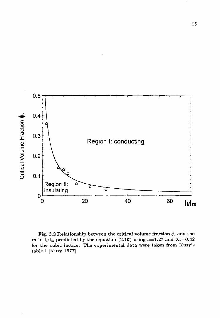
where a=1.27 and X e=0.42 for a cubic lattice. The <Pc values predicted by this model

are in good agreement with the many experimental results for Idle 2::2.0, as shown in

Fig. 2.2.

It should be noted that the two models discussed above do not account for any

" interactions", such as attractions and repulsions, between two grains and do not

apply to nonspherical grains.

A further development in the modeling of the critical volume fraction <Pc was the

introduction of the concept of the excluded volume in continuum percolation systems

[Balberg 1987b and references therein]. The excluded volume is defined as the vol

ume around an object v;'x into which the centre of another object is not allowed to

0

-e-c 0

+=i c..> co ~

u.. Q)

E :J 0 > cu c..>

+=i ·c ()

25

0.4

0.3 Region I: conducting

0.2

0.1 Region II: insulating 0

0 0 20 40 60 Ii/1m

Fig. 2.2 Relationship between the critical volume fraction cPc and the ratio ~/Ln predicted by the equation (2.16) using a=1.27 and X c=0.42 for the cubic lattice. The experimental data were taken from Kusy's table I [Kusy 1977].

26

enter, if overlap of these two permeable objects is to be completely avoided. Using

the excluded volume concept, ¢e ha3 been derived as

¢e = 1 - exp [- (Be V / < Vex > ) 1 ' (2.17)

where V is the grain volume, < Vex > the proper average of the objects' excluded

volumes, and Be the Z ~ 00 limit value of PeZ, where Z is the coordination num

ber of the lattice (see Table 2.1). Be turns out to be invariant for a given object

shape. For example, the numerical values of Be and V /Vex are Be=2.7 and 4.5, and

V /Vex=1/8 and 1/4, for spheres (3d) and disks (2d), respectively. Consequently from

Equation (2.17) ¢e=0.286 and 0.675 for spheres (3d) and discs (2d) with excluded

volume effects, respectively. Note that this is a "soft" overlapping sphere model in

contrast to the hard sphere model which gives ¢e = 0.16.

The excluded volume theory predicts that the percolation threshold also depends

on any macroscopic anisotropy of a system. The anisotropy considered arises from

the orientation distribution (partially or completely parallel to a certain direction or

plane) of nonspherical grains in space. In this case ¢e is generally larger than its

counterpart in the situation with completely random orientation, and depends both

on the aspect ratio of the particles and orientation states [Nan 1992 and references

therein].

2.3.2 Electrical Conductivity and Dielectric Constant

As in lattice percolation problems, the critical behavior of physical properties of

binary continuum percolation systems is always controlled by the single correlation

length ~, which diverges as ¢e is approached from both sides, and is given by

(2.18)

27

where ao is the mean grain size, and v is the critical exponent.

The DC conductivity of a binary conductor-insulator composite behaves in a singu

lar fashion near the critical conducting volume fraction <Pc, at which the first electrical

conducting path spanning the whole samples is formed, if Ui is zero. The DC conduc

tivity u( <p, 0) of conductor-perfect insulator composites vanishes as <Pc is approached

from the conducting side ( <Pc) as

(2.19)

where t is the conductivity exponent, which depends only on the dimensionality of

system in lattice and ideal continuum systems. Computer simulations give t=1.1 -

1.3 in two dimensions and t = 1.6 - 2.0 in three dimensions [Stauffer and Aharony

1994]. On the other hand, u( <p, 0) diverges as <p approaches <Pc from below, if U c is

infinite, as

(2.20)

where the exponent s describes the divergence behavior of conductivity on the in

sulating side. The numerical calculations suggest s= 1.1 - 1.3 in two dimensions

and s=0.7 - 1.0 in three dimensions [Nan 1993 and reference therein]. When the

conductivity ratio of real continuum conductor-insulator percolation systems is finite,

the so-called crossover (critical) region is defined as

(2.21 )

Here the DC conductivity can be shown to be constant [Straley 1977 and Kirkpatrick

1979], as

(2.22)

The low frequency dielectric constant c( <p, 0) of percolation systems diverges as

(2.23)

28

where 8 is the dielectric exponent, and ¢>c ~ ¢>. The scaling ansatz predicts 8 = S

[Nan 1993].

The AC conductivity a( ¢>, w) and dielectric constant c( ¢>, w) for a percolation

system have been studied using the scaling ansatz with a complex AC conductivity

E(¢>,w) = a(¢>,w) + jWE(¢>,W) [Efros and Shklovskii 1976, Bergman and Imry 1977,

Straley 1977, Stephen 1978, Webman 1981, Stroud and Bergman 1982, Wilkinson et

al. 1983, and Clerc et al. 1990]. The form of this scaling equation is

t (JW) E(¢>,w)ex:I¢>-¢>cI9± We ' (2.24)

where j = vi=T, 9+ and 9_ are two different scaling functions for above and below

¢>c respectively, and We is the critical frequency given by

(2.25)

Here q is an exponent, expected to be (t + 8)lt on the conducting side and to be

-( t + 8) Is on the insulating side of percolation. At ¢> = ¢>c and at low frequencies,

(2.24) reduces to

where

Defining

(jW)X

E(¢>c,w) ex: We '

t x---8+(

8

Y=8+(

The analytic properties of Equation (2.26) then lead to

(2.26)

(2.27)

(2.28)

(2.29)

29

and

(2.30)

where x and yare critical exponents. It is easily to see from (2.27) and (2.28) that

the critical exponents x and y satisfy the following scaling relation

x+y=l. (2.31)

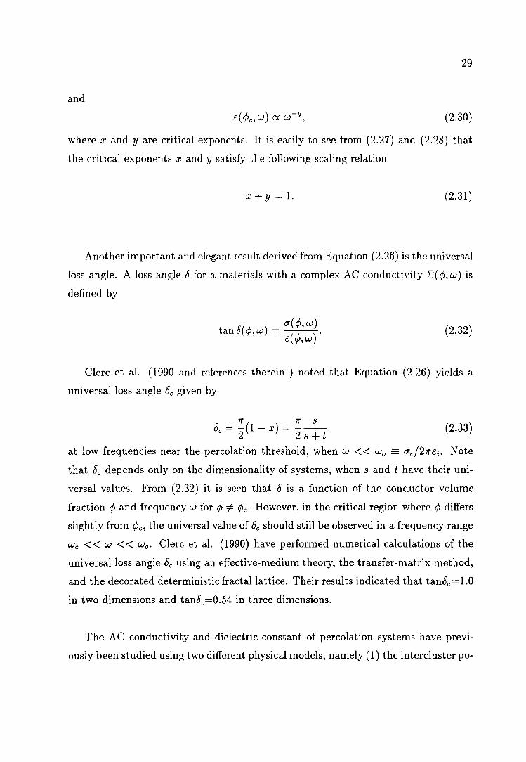
Another important and elegant result derived from Equation (2.26) is the universal

loss angle. A loss angle b for a materials with a complex AC conductivity ~(<p, w) is

defined by

u(<p,w) tanb(<p,w) = c(<p,w)' (2.32)

Clerc et al. (1990 and references therein) noted that Equation (2.26) yields a

universal loss angle be given by

7r 7r S b =-(l-x)=--

e 2 2s+t (2.33)

at low frequencies near the percolation threshold, when w « Wo _ Ue/27rci. Note

that be depends only on the dimensionality of systems, when sand t have their uni

versal values. From (2.32) it is seen that b is a function of the conductor volume

fraction <p and frequency w for <p =1= <Pe. However, in the critical region where <p differs

slightly from <Pe, the universal value of be should still be observed in a frequency range

We « w «Wo. Clerc et al. (1990) have performed numerical calculations of the

universal loss angle be using an effective-medium theory, the transfer-matrix method,

and the decorated deterministic fractal lattice. Their results indicated that tanbe=l.O

in two dimensions and tanbe=0.54 in three dimensions.

The AC conductivity and dielectric constant of percolation systems have previ

ously been studied using two different physical models, namely (1) the intercluster po-

30

larization model [Bergman and Imry 1977], also known as R-C model [Clerc et al. 1990]

and (2) the :tnomalous diffusion model ~Gefen et al. 1983]. A1.though these two theo

ries are based on different starting assumptions, they both predict the scaling relations

(2.29)' (2.30) and (2.31) but differ in the expressions they predict for the exponents

x and y.

In the intercluster polarization model, the conducting component is considered

as "pure" conductor while the insulating component is identified as perfect dielec

tric. Within the framework of intercluster polarization, Efros and Shkolovskii (1976),

Bergman and Imry (1977), Stroud and Bergman (1982), Webman (1981), and Wilkin

son et al. (1983), derived the relations (2.27) and (2.28). In fact the percolation equa

tions for the electrical conductivity, dielectric constant and dielectric loss, discussed

above, all belong to the intercluster polarization picture.

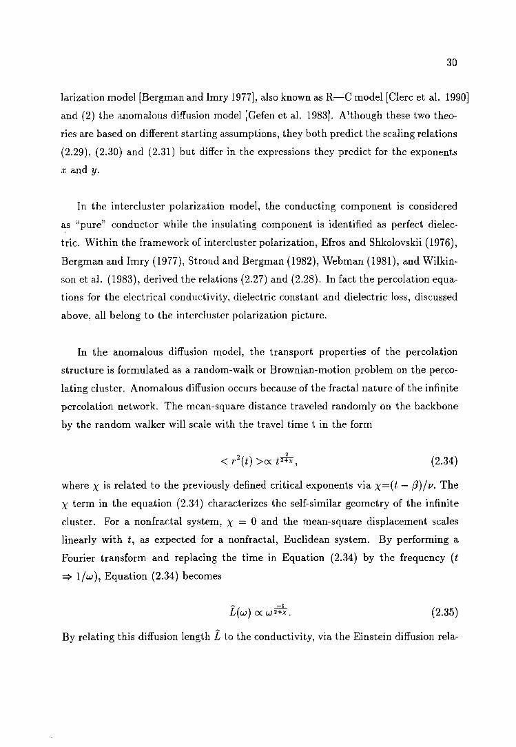
In the anomalous diffusion model, the transport properties of the percolation

structure is formulated as a random-walk or Brownian-motion problem on the perco

lating cluster. Anomalous diffusion occurs because of the fractal nature of the infinite

percolation network. The mean-square distance traveled randomly on the backbone

by the random walker will scale with the travel time t in the form

(2.34)

where X is related to the previously defined critical exponents via X=(t - (3)/v. The

X term in the equation (2.34) characterizes the self-similar geometry of the infinite

cluster. For a nonfractal system, X = 0 and the mean-square displacement scales

linearly with t, as expected for a nonfractal, Euclidean system. By performing a

Fourier transform and replacing the time in Equation (2.34) by the frequency (t

'* l/w), Equation (2.34) becomes

~ -1

L(w) cx:w2+x. (2.35)

By relating this diffusion length L to the conductivity, via the Einstein diffusion rela-

31

tion, and averaging over the contributions of the charge carriers in different clusters,

Gefen et al. (1983) calculated the dispers;on for electrir:al conductivi ~y and dielectric

constant, and obtained

t x=----

211 - f3 + t'

211 - f3 y=

211 - f3 + (

(2.36)

(2.37)

Note that these exponents x and y also obey the scaling relation (2.31), because a

single time scale for both resistance and capacitance is assumed in the calculation.

More recently, (2.36) and (2.37) have been derived using, instead of the generalized

Einstein relation, the Miller-Abrahams equivalent network which has the same elec

trodynamic behavior as the random-walk system [Schirmacher 1994]. No model exists

which unifies the intercluster polarization and anomalous diffusion mechanisms.

2.3.3 GEM Equation

In Subsection 2.3.2, separate equations, (2.19) and (2.20), have been used to

describe the DC conductivities of a percolation system on each side of critical volume

fraction. McLachlan (1986 and 1996) developed a generalized effective media (GEM)

equation, which can, however, be used to fit the conductivity data obtained from

percolation systems. This equation can be written as

(1 - <p)( (}"V' - (}"l/s) + <p( (}"~/t - (}"l/t) = 0, l/s + l-t/>c l/s l/t +!.::.!e£ l/t (2.38)

()" i ~ ()" ()" c t/>c ()"

where the symbols have their usual meaning. This equation is a continuous interpo

lation between the two percolation equations (2.19) and (2.20), which describe the

divergent behavior of conductivity near the percolation threshold. When (}"i=O, the

GEM equation reduces to

( <P - <PC)t

()" = ()" C 1 - <Pc ' (2.39)

32

and when O"c=OO, it reduces to

(2.40)

Both of these equations have the mathematical form of the percolation equations.

Letting C/>C = 0 in Equation (2.39) and C/>C = 1 in (2.40), one arrives at the Bruggeman

asymmetric equations. Furthermore, in the case of t=s=l, the GEM equation reduces

to the Bruggeman symmetric equation.

The GEM equation has been used to accurately fit the conductivity data for

a number of binary percolation composites [McLachlan et al. 1990 and references

thereinJ. It has also been shown [Deprez et al. 1988J that the electrical conductivity,

thermal conductivity and permeability can all be fitted to the GEM equation with

the same two morphology parameters C/>C and t=s.

2.3.4 Hall Coefficient and Magnetoresistance

The magnetoresistance and Hall coefficient of percolation systems involve the

coupling of electrical and magnetic fields, and have been less thoroughly investi

gated than the electrical conductivity and dielectric constant. For the magnetoresis

tance, Bergman (1987) calculated, using the scaling ansatz, the magnetoconductivity

6.0" (H) and the relative magnetoresistance [R(H)-R(O)J/ R(O) in low magnetic fields,

near the critical volume fraction. Bergman's is the only theory for magnetoresistivity

and as only the transverse magnetoresistances of the G-BN conducting parallelepiped

samples are measured in this thesis, the critical behavior of the transverse magne

toresistance in conducting regime is quoted first. Bergman (1987) gave

6.R = R(H) - R(O) ('" _ '" )tm-t R R(O) ex 'f' 'f'c ,

(2.41 )

and

- 6. 0" = -[O"(H) - O"(O)J ex (c/> - c/>c)tm, (2.42)

33

where tm is the critical exponent describing the critical behavior of the second order

Hall contribution to the low field m:1gnetoresistance, and H is the magnetic field.

Bergman (1987) also made the prediction that t = tm , implying that the relative

magnetoresistance [R(H) - R(O)]I R(O) is constant near the percolation threshold.

Many authors [Skal and Shklovskii 1974, Levinshtein et al. 1975 and Straley 1980]

have predicted that the Hall coefficient RH of a percolation system diverges, as the

critical volume fraction ¢c is approached from the conducting side of the percolation

transition, as

(2.43)

Here 9 is the "Hall" critical exponent with predicted values of 0.5 - 0.6 in three di

mensions and 9 = 0 in two dimensions. However, according to Bergman and Stroud

(1985), the effective Hall coefficient RH of conductor-insulator composite on the con

ducting side can be described by scaling theory, as

(2.44)

where Rc and Ri are the Hall coefficients of the conductor and insulator respectively

and t is the conductivity exponent defined in Subsection 2.3.2. The theoretical values

of the exponent 9 in Equation (2.44) are 9=0 in two dimensions and 9=0.31"V0.8 for

three dimensional systems. The second term dominates the right-hand side of (2.44)

only when ¢ is close enough to <Pc for the condition

(2.45)

to be satisfied. Dai et al. (1987) investigated experimentally the exponents t and 9

for the AI-Ge films and found that the measured values of t=1.75 and 9 =3.8 (~2t)

and 0.38, close to the threshold of Al and the threshold of Ge respectively, are in

good agreement with Equation (2.44).

34

2.3.5 1/ f (flicker) Noise

The voltage drop across almost any resistor fluctuates about its average value with

or without a constant current flowing through it. In the absence of a driving current,

these voltage fluctuations are known as Johnson or Nyquist noise, which originates

from the thermal motion of the charge carriers. In an equilibrium situation this

thermal motion has an average energy 3/2kBT, where kB is the Boltzman's constant

and T is the absolute temperature. The power spectrum Sv(J) (J=frequency) of the

voltage fluctuations is related to its resistance R, through a fluctuation-dissipation

theorem, by

Sv(J) = 4kBTR. (2.46)

Since the relaxation time of thermal motion is extremely fast, 7=10-12S, the Johnson

noise is frequency independent ( or white) at low frequencies ( < 1012 Hz).

When a DC current is passing through a resistor two "excess" noises, depending

upon the magnitude of the DC current, are often observed. The first of these is shot

noise. Its spectral density SI(J) of the current fluctuations is also "white" or constant

at low frequencies and is given by

Sr(J) = 2eI, (2.4 7)

where e is the electronic charge, and I is the DC current flowing through the sample.

The shot noise arises because of the finite size of the electrical charge carriers which

leads to current pulses at the electrodes of the sample. In practice, the shot noise

is large only at low current where the discreteness of the electrical charge carriers

is important. The details of the transport processes of the charge carriers have no

influence on the shot noise, provided there is no interaction between them and their

statistics are close to Boltzman [Hooge et al. 1981].

At sufficiently low frequencies, the "1/ f" or "flicker" noise is the dominant excess

noise. Unlike the Johnson noise and the shot noise, which are well understood, the

35

source of 1/ f noise has been the subject of innumerable controversies [Dutta and Horn

1981, Hooge, Kleinpeening, and Vandamme 1981 and Weissman 19'38 J. Hooge (1969)

proposed an empirical formula for the 1/ f noise in homogeneous samples, which in

terms of the voltage fluctuations can be written in a general form as:

O'V19

Sv(J) = NrJ f'Y' (2.48)

where, in Hooge's original paper, 0' is a dimensionless constant, with a value of

about 2 x 10-3 for 111-V compound semiconductors and not greatly dependent on

the temperature, 19=2 for ohmic samples, 1]=1, I is a number close to unity over a

wide frequency range typically from 10-2 Hz to 104 Hz, and N the total number of

charge carriers; usually proportional to the sample volume. In more recent years,

the observed value of 0' has been found to vary from 10-5 to 10-1 in small volume

metallic samples [Testa et al. 1988J and to be as high as 103 to 107 in granular high

T c superconductors [Song et al. 1990J. Although the relation between the noise power

and DC voltage is usually given by the square-law, i.e., 19=2, for most electrical 1/ f noise systems, a linear dependence of Sv(J) on V, for a limited DC current range, has

very recently been observed in superconductors [Kang et al. 1994J. The exponent I

is usually found to be 1. 0±0.1 over six or more decades of frequency. However, a great

controversy over the factor N still exists. The inverse dependence on N was postulated

by Hooge (1969) to unify the noise process in metals and semiconductors with 0' ~

2 X 10-3 . The physical idea behind this postulate is that independent fluctuations are

occurring on each of the mobile carriers, that is, the noise process for each carrier is

independent.

For an ohmic resistor, the voltage fluctuation 8V under a constant bias current

arises from resistance fluctuations 8R, and 8V = 18R. In this case, the normalized

spectrum is independent of the type of stimulation, e.g. constant current or voltage,

and [Hooge et al. 1981 J

Sv(J) _ SR(J) _ S/(J) __ 0'_

V2 - R2 - /2 - NrJ f'Y . (2.49)

36

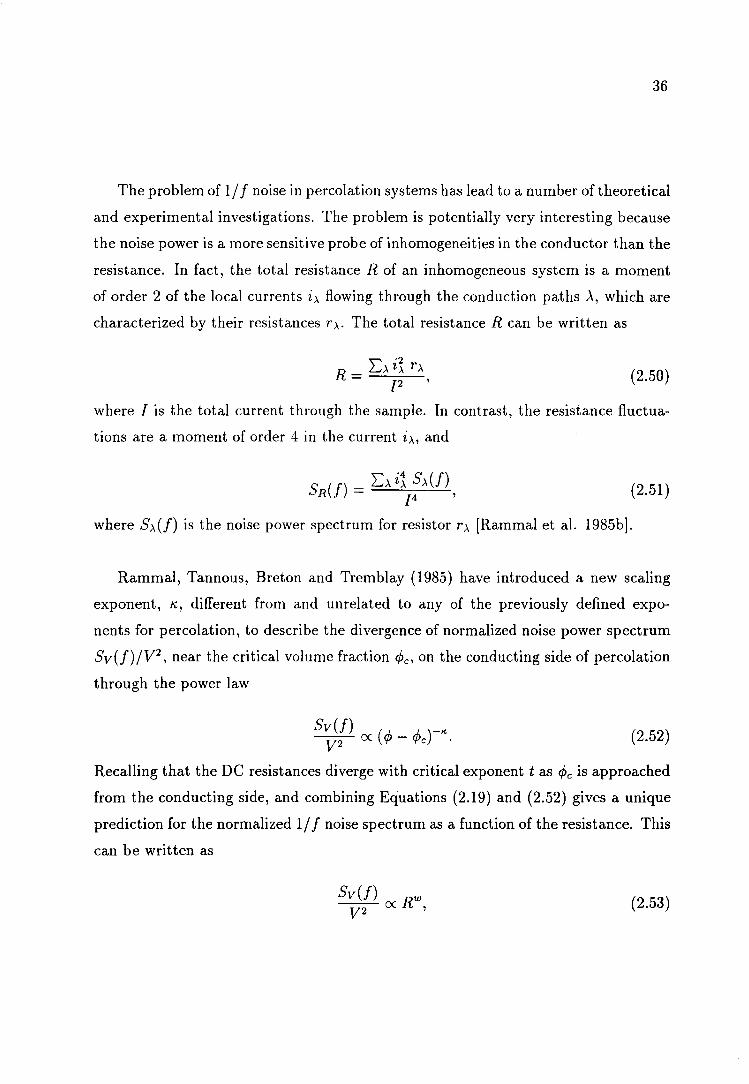
The problem of 1/ f noise in percolation systems has lead to a number of theoretical

and experimental investigations. The problem is potentially very interesting because

the noise power is a more sensitive probe of inhomogeneities in the conductor than the

resistance. In fact, the total resistance R of an inhomogeneous system is a moment

of order 2 of the local currents i>. flowing through the conduction paths A, which are

characterized by their resistances r>.. The total resistance R can be written as

(2.50)

where I is the total current through the sample. In contrast, the resistance fluctua

tions are a moment of order 4 in the current i>., and

(2.51 )

where S>.(f) is the noise power spectrum for resistor r>. [Rammal et al. 1985b].

Rammal, Tannous, Breton and Tremblay (1985) have introduced a new scaling

exponent, K, different from and unrelated to any of the previously defined expo

nents for percolation, to describe the divergence of normalized noise power spectrum

Sv(f)/V2, near the critical volume fraction <Pc, on the conducting side of percolation

through the power law

Sv(f) (,I., _ ,I., )-K. V2 ex: 'P 'Pc . (2.52)

Recalling that the DC resistances diverge with critical exponent t as <Pc is approached

from the conducting side, and combining Equations (2.19) and (2.52) gives a unique

prediction for the normalized 1/ f noise spectrum as a function of the resistance. This

can be written as

Sv(f) RW lf2 ex: , (2.53)

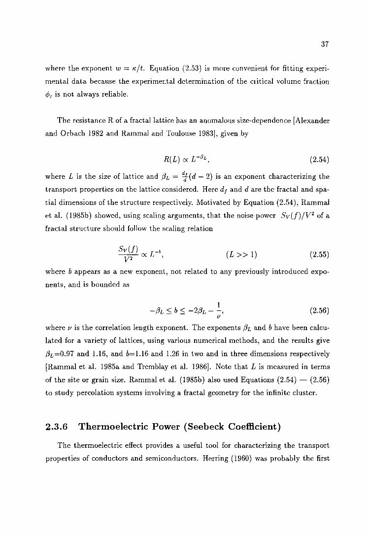
37

where the exponent w = ;;,ft. Equation (2.53) is more convenient for fitting experi

mental data because the experimedal determin .. tion of the clitical volume !raction

<Pc is not always reliable.

The resistance R of a fractal lattice has an anomalous size-dependence [Alexander

and Orbach 1982 and Rammal and Toulouse 1983], given by

(2.54)

where L is the size of lattice and (3L = 1-( d - 2) is an exponent characterizing the

transport properties on the lattice considered. Here df and d are the fractal and spa

tial dimensions of the structure respectively. Motivated by Equation (2.54), Rammal

et al. (1985b) showed, using scaling arguments, that the noise power Sv(f)fV2 of a

fractal structure should follow the scaling relation

S~!) <X L-b, (L» 1) (2.55)

where b appears as a new exponent, not related to any previously introduced expo

nents, and is bounded as

1 -(3L ::; b::; -2(3L - -,

v (2.56)

where v is the correlation length exponent. The exponents (3L and b have been calcu

lated for a variety of lattices, using various numerical methods, and the results give

(3L=0.97 and 1.16, and b=1.16 and 1.26 in two and in three dimensions respectively

[Rammal et al. 1985a and Tremblay et al. 1986J. Note that L is measured in terms

of the site or grain size. Rammal et al. (1985b) also used Equations (2.54) - (2.56)

to study percolation systems involving a fractal geometry for the infinite cluster.

2.3.6 Thermoelectric Power (Seebeck Coefficient)

The thermoelectric effect provides a useful tool for characterizing the transport

properties of conductors and semiconductors. Herring (1960) was probably the first

38

to study this problem for composites, but only where the differences in the physical

quantiti~s b~tween the various components were assumed to be small. Webman et

al. (1977) studied the thermal conductivity and the thermoelectric power of binary

inhomogeneous materials consisting of conductor and nonconductor components with

electrical conductivities U c and Ui, thermal conductivities f{c and f{i, and Peltier

coefficients Pc and Pi respectively. They derived a self-consistent effective-medium

approximation for the thermoelectric power, which can be written as

where

and

6f{m < S'D' > Sm = ------------

1 - 3 < f{' D' > '

S'= p'. u'

(2.57)

(2.58)

(2.59)

Here the subscript m refers to composite materials having a thermoelectric power

Sm, an effective electrical conductivity U m and an effective thermal conductivity f{m.

p', u' and f{' are the local Peltier coefficient, electrical conductivity and thermal

conductivity, respectively; and the average < - > was taken over all space or over all

local configurations around a given point.

Equation (2.57) exhibits two interesting features. First, in the case where Ui ~ Uc

and Pi ~ Pc, it reduces to

(2.60)

where ¢> > ¢>c+0.1, that is, well above the percolation threshold, Sm(¢» is independent

of ¢>.

Second, in the insulating region, ¢> < ¢>c, Sm (¢» shows a pronounced rise with

decreasing ¢>, given by

39

(2.61 )

provided that O'i ~ O'e, Si ~ Se, and I( ~ Ke. In summary, Sm(<P) is proportional to

0'-1 (<p) below <Pc and is constant above it.

More recently Milgrom and Shtrikman (1989) and Bergman and Levy (1991) made

theoretical studies of thermoelectric properties of binary composites, using the field

decoupling transformation discovered by Straley (1981). They obtained an expression

for the effective thermoelectric power of binary composites, given by

(2.62)

where the symbols have the meanings already given in this section. Starting from

this equation, the thermoelectric power Sm of composites can be expressed in a form

showing an explicit interpolation between the thermoelectric power values of the

metallic component Se and insulating component Si, which is

(2.63)

The behavior of Sm near a percolation threshold has been studied in detail, using

the scaling arguments, by Levy and Bergman (1992). In their scaling scheme, both

Ki/ Ke and O'i/O'e are assumed to be very small compared to unity. Furthermore, the

dependence of Sm upon both the electrical conductivity ratio O'i/ O'c and the thermal

conductivity ratio Ki/ Kc, which can sometimes be described by qualitatively different

expressions of <p, can make the scaling behavior very complex, in contrast to the

familiar simple power-law for the electrical conductivity. It is surprising that the

coupling of electric and temperature fields does not cause the appearance of any new

exponent, necessary to describe the critical behavior of thermoelectric power, as Levy

and Bergman could use only the exponents t and s to achieve their objectives. For

graphite and hexagonal boron-nitride, one has Ki 2: Kc [Lide 1994]. Therefore Levy

and Bergman's scaling scheme for thermoelectric power of percolation systems is not

40

applicable to the G-BN systems. New power-laws for the thermoelectric power near

percolation threshold are proposed in th~s thesis and will be presented in Chapter

SIX.

2.4 The Nonuniversality of Critical Exponents

The applications of the scaling laws of lattice percolation to continuum systems,

as discussed in Section 2.3, are probably attributed to the concept of the universality

of the scaling behaviors, i.e. they depend only on the dimension of the percolation

system, and do not on the details of geometric structure or the interactions between

the conducting particles. For the critical exponents sand t, the most widely accepted

universal values in three dimensions are 0.87 and 2.0 respectively. Although many

computer simulations and experiments support this belief, some experimental results

on continuum systems have shown that the value of exponent t can be 3 or even

larger [Pike 1978, Carmona et al. 1984, Chen and Chou 1985, and McLachlan et al.

1990], which implies that the critical exponents are not necessarily universal in some

continuum systems.

Kogut and Straley (1979) first realized that peculiar conductance distributions

in an infinite percolation resistor network could yield nonuniversal conductivity ex

ponents. Consider a network where the conductances of the occupied sites are dis

tributed according to the distribution function h( G) '" G-Of as G --+ 0 for G < Ge ,

where O<a<1. The value Ge is defined as the minimum conductance in a subset of

conductances, which give rise to percolation when the conductances are placed into

the lattice in descending order. Since close to the percolation threshold, the resis

tance of the sample is determined by the intercluster links, and the total resistance

of a link is determined largely by a series connection of the resistors G-I, the average

conductance of the system is given by

(2.64)

Therefore the universal exponent t should be replaced by

, { t t -t+~

1-01

if a < 0

if 0 < a < 1.

41

(2.65)

Note that this model does not allow t' to be smaller than the accepted universal

values of t. The first percolation system found, that yielded a theoretical distribu

tion function of the G-OI class, leading to nonuniversal behavior of the conductivity,

was the 'Swiss-cheese' (or random-void) model [Halperin et al. 1985]. In this sys

tem, uniformly-sized overlapping insulating spheres are placed randomly in a uniform

conducting matrix. Near the percolation threshold <Pc, the resistance behavior of the

Swiss-cheese model is dominated by the narrow conducting necks which join the larger

regions of the conducting medium. The local conductance G of these narrow necks

depends on their neck 'width' 8 as G '" 8Y+l, where y = a/(l - a). For y 2': 0 or

O<a ~ 1, the critical exponent is in the range

Max[y+l+(d-2)1I, t] ~ t' ~ t+y. (2.66)

For y ~O or a ~O, i.e. in the inverted Swiss-cheese model, the roles of the two com

ponents are interchanged. A similar argument, analogous to the Swiss-cheese model,

can then be made. However, in this case the conductance distribution does not result

in any correction to the conductivity exponents.

Balberg (1987a) suggested another system which gives nonuniversal behaviour. In

this system, the conducting particles are embedded in an insulating matrix, similar to

the inverted Swiss-cheese model, but where the inter-particle conduction mechanism

is tunneling and the particles are arranged onto a percolating network. In this model,

the tunneling conductance between two hard spherical conducting particles of radius

bo , separated by a distance r (»bo), is given by

G ex exp( -r/l), (2.67)

where I IS the tunneling distance (typically lO",lOOA). To find the conductance

42

distribution, a distribution function for the distance between the surfaces of two

adjacent particles, h(r), was pro~osed. This is

(2.68)

where ao is the average closest distance between two particles. Using the relation in

elementary probability theory h(G) = h(r)· drjdG, for large values of r, Equations

(2.67) and (2.68) give rise to the distribution G( alo )-1 = G-a for small G, yielding a

nonuniversal critical exponent

(2.69)

The nonuniversality of the conductivity exponent t has also been found in per

colation systems with macroscopic anisotropy [Yoon and Lee 1990; Carmona et al.,

1984]. More recently, Lin (1991) found in the PrBa2Cu307-Ag percolation system,

that the conductivity exponent t increases monotonically from 1.48 to 1.91 with in

creasing conductivity ratio acjai, from 3.2x104 to 2.2x1011. The mechanisms for the

breakdown of the universality of t in these last two cases are not well understood.

43

Chapter 3

APPARATUS AND

EXPERIMENTAL METHODS

3.1 Sample Fabrication

All the samples studied in this thesis are mixtures of Graphite powder (G: Lonza,

KS75) as the conducting component and hexagonal Boron-Nitride powder (BN: Ad

vanced Ceramic Corporation) as the insulating component. Since the actual bulk

resistivity of the graphite and BN powders, and the actual dielectric constant of the

BN powder, used in the present study, are not known, they had to be measured ex

perimentally, as will be described in this chapter. Compressed pellets of the BN have

a resistivity of 10160 - em in the axial direction and 4.2 x 10140 - em in the trans

verse direction, and a relative dielectric constant of 2.8 in the axial direction. Similar

compressed Graphite pellets have a resistivity of 0.120 - em and 2.9x10-3 0 - em

in the axial and transverse directions respectively. This measured axial resistivity is

consistent with that of 0.15 '" 0.250 - em along the c-axis observed in a good single

graphite crystal at room temperature, while the measured transverse resistivity is

close to that of 4.2x 10-5 0 - em in the a-b plane [Reynolds 1968]. Therefore the

measured bulk graphite resistivity is thought to be mainly bulk resistivity of graphite

grains and not intergrain contacts.

44

Two classes of powder mixtures were made using these materials: the first, com

pressed discs and parallelepipeds cut from the discs, :tnd the second, a powder mixture

undergoing compression. In this section, the relevant details of the method of sample

preparation and fabrication are discussed.

A predetermined amount of graphite and BN powder was weighed out with the ap

propriate weight percentage of the two components. This weight percentage is equal

to the relative volume percentage, since these two constituents have the same densi

ties: 2.25gms/cm3 [Lide 1994]. The preweighted amounts of G and BN powder were

then put into an agate container, together with agate balls, and ground and mixed

in a planetary mill. At the end of this process, the powders had become a random

mixture of grains, since the two constituents are mechanical isomorphs, with the same

crystal structure (hexagonal) and almost the same crystal structure parameters, as

discussed in Chapter one. Carefully poured 50%G-50%BN and 55%G-45%BN powder

mixtures, with a total weight of 35gms each, were used in this form for conductivity

and dielectric constant measurements, in the appropriate sample cell. To make the

compressed discs, about 3gms of the appropriate powder mixture was poured into

a die of 26mm diameter and compressed into a disc using a pressure of 200MPa.

The discs were typically about 2.5mm thick. Bar shaped samples (50x5x5mm) were

also made, using a square cylinder with a cross-section of 50x5mm and a pressure of

200MPa, perpendicular to the 50x5mm surface.

For the measurements of the axial conductivity, dielectric constant and 1/ f noise,

silver colloid paste was painted on two surfaces of the discs, forming both the elec

trodes and capacitor plates. During this procedure a circle of thin copper wire, with

a diameter of about 16mm for the current/voltage contacts, was embedded in the

electrodes. For samples with a resistance less than lOOn, a separate wire near the

centre of the disc, for a separate voltage contact, was also embedded in the elec

trodes. When all the measurements in the axial direction were finished, the silver

paste was stripped off the faces of the discs and the discs were cut and polished into

24(length)x8(width)x2(thickness)mm and 18x3x2mm parallelepipeds. The former,

45

using silver paste and embedded copper wire on the two 8x2mm surfaces as electrical

contacts, were used for the IPeasnrements of the transverse DC conductivity, Hall

coefficient, 1/ f noise and thermoelectric power. The smaller parallelepipeds, with

the electrical contacts on the two 18x2mm opposite surfaces, were used only for the

transverse magnetoresistance measurements, which are described in Section 3.4.

Because of the slow relaxation after mechanical compression, it was found that

the resistance of the disc samples, especially those near the percolation threshold,

increased with time, so that an aging period was allowed before performing the various

measurements on these samples. In an effort to determine the correct aging time, the

resistance of the sample with d> =0.156 was measured twice daily for a period of 35

days. The results are plotted in Fig. 3.1, in which the solid curve is a best fit to the

data using the following equation

(3.1)

where Rl is the initial (t=0) resistance, t is time, and 7 is the relaxation time.

For this particular sample, a least squares fit gave Rl =73.7H!, R2 = 38.4k!1 and

7 = 20.5days. For 99% accuracy of the final resistance R( t = 00), a simple calculation

based on Equation (3.1) shows that minimum aging time tmin = 3.57 = 72days is

required. All the measurements reported in this thesis were made on disc samples

that had aged for at least three months. Samples measured a year later were found

to have altered by less than 1 %.

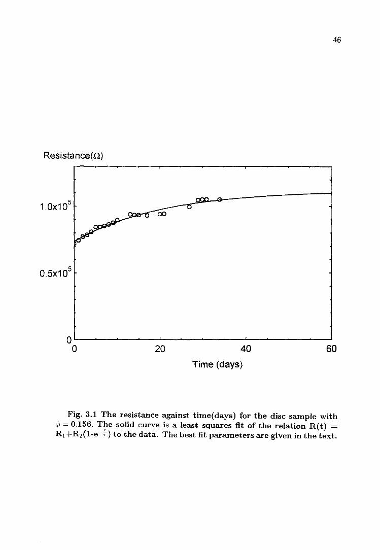
Resistance(n)

5 1.0x10

5 0.5x10

OL-~--~--~~--~~--~--~~--~--~~

46

o 20 40 60

Time (days)

Fig. 3.1 The resistance against time(days) for the disc sample with IjJ = 0.156. The solid curve is a least squares fit of the relation R( t) = R 1+R2 (1-e-;) to the data. The best fit parameters are given in the text.

47

3.2 Sample Characterization

3.2.1 Porosity of the Disc Samples

The apparent densities of disc samples were obtained by measuring their mass

and thickness only, as their diameters were constant (26.0mm). The porosity of the

discs is calculated using the formula

w porosity = 1 - 2

P 6, 1fT •

where

W = the mass of disc, grams;

w = 1 - 0.0838 6,

p= the density of disc without porosity, 2.25gjem3;

r= the radius of disc, 1.30cm;

~ = the thickness of disc, em.

(3.2)

Fig. 3.2 shows the results of these measurements in the form of disc porosity

against the volume fraction of graphite. As the mass of the discs can be measured

with uncertainty of ±O.lmg in the total mass of about 2.5g, the experimental error

in porosity comes mainly from the thickness measurements which have 2% relative

error. Therefore the error bars for the porosity data in Fig. 3.2 are all less than

the size of the symbols. It is seen from this plot that the average porosity is about

18% for all the compressed disc samples, this is consistent with previous results on

pure graphite measured using a similar method [Reynolds 1968]. Furthermore, near

the percolation threshold <7>c=0.150 (see Chapter 4) there is a small peak of porosity.

This could possibly be attributed to the fractal structure of the infinite percolation

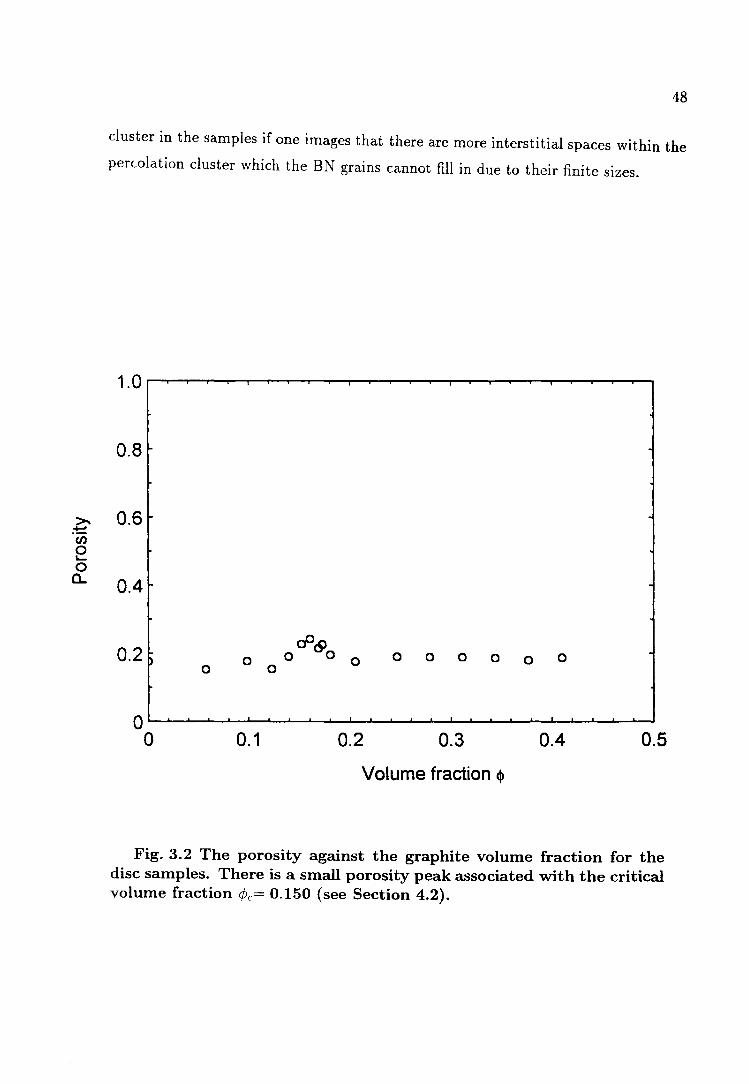
>-~ en 0 ~

0 a..

48

cluster in the samples if one images that there are more interstitial spaces within the

percolation cluster which the BN grains cannot fill in due to their finite sizes.

0.8

0.6

0.4

0.2 ~ ~c9

0 0 o 0 0 0 0 0 0 0 0 0

o~~~~~~~~~~~~~~~~~~~~

o 0.1 0.2 0.3 0.4 0.5

Volume fraction cj)

Fig. 3.2 The porosity against the graphite volume fraction for the disc samples. There is a small porosity peak associated with the critical volume fraction ¢c= 0.150 (see Section 4.2).

49

3.2.2 X-ray diffraction

X-ray diffraction (XRD) was principally used to examine the grain orientation in

the discs. A Phillips PW 1010 X-ray diffraction spectrometer was used and operated

at 40kv, 20ma, and a scanning rate of 10/ minute. A nickel filter was placed in po

sition so as to produce nearly monochromatic radiation from a copper source. The

results are shown in Fig. 3.3. As graphite and hexagonal BN have the same crystal

structure and nearly the same parameters and density, they are indistinguishable by

the usual X-ray methods. Therefore, any detectable impurity should show up as un

expected peaks in the traces of graphite and/or BN. The traces in Fig. 3.3 show that

no significant contamination was introduced during sample preparation.

To monitor the grain orientation or anisotropy in the powders and discs, a powder

mixture was poured into a copper cup of 26mm in diameter and 4mm in depth. The

powder always filled the cup and the X-rays scanned the flat upper surface. Different

densities of powder in the cup were obtained by pressing the top surface using a

piston with the same diameter as that of the copper cup. A filling and pressing

process was repeated until the desired density was obtained. The relative intensity

of peaks changed accordingly with the apparent density of the powder in the cup, as

shown in Fig. 3.4. The X-ray trace of a lightly poured and unpressed powder was

treated as the reference, i.e. grains distributed randomly without any orientation.

The anisotropy of discs with the same compositions was determined by comparison

with the reference. The results and calculations indicate that the Graphite and BN

crystals in the discs have about 80% of their c-axis within 10 of the direction of the

pressure or axis of the disc. This orientation effect is later qualitatively confirmed

from the very anisotropic resistivity measured in the compressed samples.

,-. . o . < '-"

~ .... til c: CD

= ~

,-. . R < '-"

~ .... ~ CD

-= ~

f--/' ~ 20

(a) cjJ = 0.00

20

(b) ¢ = 0.82

A

125 105

125° 1050

j

J \ ~ -" ~ f--.) ~ -./ '---/ - ,- - r----- -

85 6n 45 25"

j

85° 65 45° 25"

Fig. 3.3 X-ray scattering data on the disc samples with the graphite volume fractions indicted on each curve.

5°

5°

CJl o

-. . :;J . -< --.0 .... ~ Q)

1: ~

20 55° 45° 35° 25" 55°

(a)

I

I u l-, -- M

45° 35° 25° 55° 45" 35°

(b) (c)

Fig. 3.4 Comparison of X-ray scattering data of the G-BN powder with decreasing pressure from (a) to (c).

The densities of the samples from (a) to (c) are 1.81g/cm3, O.76g/cm3 and O.34g/cm3 respectively.

25()

en ~

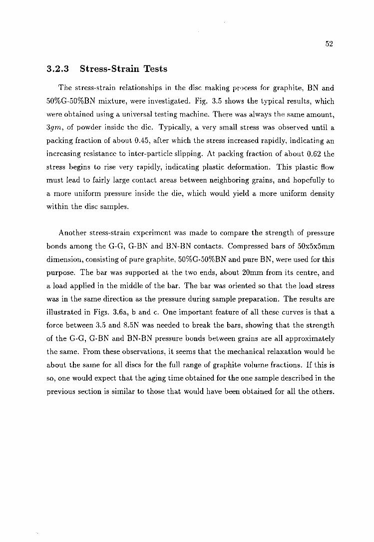
52

3.2.3 Stress-Strain Tests

The stress-strain relationships in the disc making process for graphite, BN and

50%G-50%BN mixture, were investigated. Fig. 3.5 shows the typical results, which

were obtained using a universal testing machine. There was always the same amount,

39m, of powder inside the die. Typically, a very small stress was observed until a

packing fraction of about 0.45, after which the stress increased rapidly, indicating an

increasing resistance to inter-particle slipping. At packing fraction of about 0.62 the

stress begins to rise very rapidly, indicating plastic deformation. This plastic flow

must lead to fairly large contact areas between neighboring grains, and hopefully to

a more uniform pressure inside the die, which would yield a more uniform density

within the disc samples.

Another stress-strain experiment was made to compare the strength of pressure

bonds among the G-G, G-BN and BN-BN contacts. Compressed bars of 50x5x5mm

dimension, consisting of pure graphite, 50%G-50%BN and pure BN, were used for this

purpose. The bar was supported at the two ends, about 20mm from its centre, and

a load applied in the middle of the bar. The bar was oriented so that the load stress

was in the same direction as the pressure during sample preparation. The results are

illustrated in Figs. 3.6a, band c. One important feature of all these curves is that a

force between 3.5 and 8.5N was needed to break the bars, showing that the strength

of the G-G, G-BN and BN-BN pressure bonds between grains are all approximately

the same. From these observations, it seems that the mechanical relaxation would be

about the same for all discs for the full range of graphite volume fractions. If this is

so, one would expect that the aging time obtained for the one sample described in the

previous section is similar to those that would have been obtained for all the others.

-ro 0--Q) L. ::l IJJ IJJ

~ 0-

53

1.Sx108

1.0x108

O.5x108

1 2 3 4 Strain(mm)

Fig. 3.5 A typical relationship of stress-strain in the disc making· process. T: the packing fraction=0.45; 1'1: the packing fraction =0.62.

5

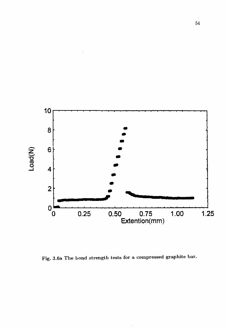
54

8 • • • - 6 • z -'U • co

0 4 • ...J

• • 2 • -,

• 0 0 0.25 0.50 0.75 1.00 1.25

Extention(mm)

Fig. 3.6a The bond strength tests for a compressed graphite bar.

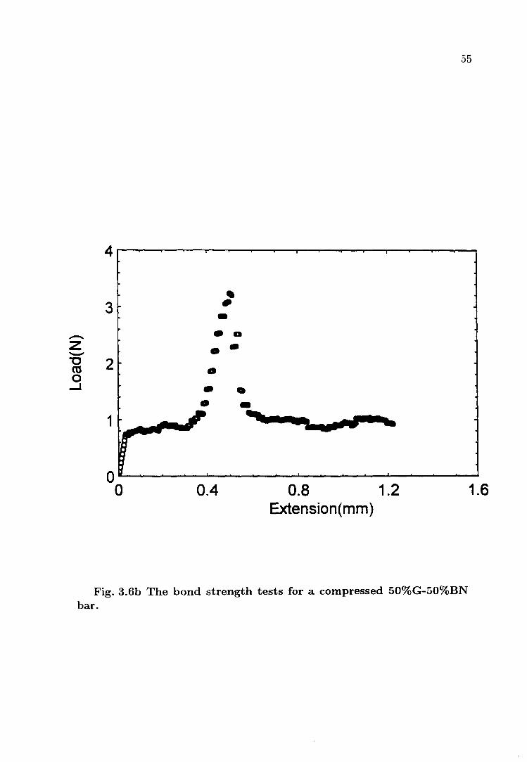
55

• 3 • -- • a

Z • • -"C 2 CO • 0 --1 • • •

1 .. o----~~--~--~~--~~~~--~~~~~

o 0.4 0.8 1.2 1.6 Extension(mm)

Fig. 3.6b The bond strength tests for a compressed 50%G-50%BN bar.

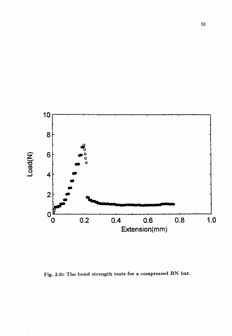
56

8

~ - 6 .0 z - 0

"0 co _ 0

0 4 • ....J

• •

2 • • " 0

0 0.2 0.4 0.6 0.8 1.0 Extension(mm)

Fig. 3.6c The bond strength tests for a compressed BN bar.

57

3.2.4 Grain Size Distribution and Shape

The grain 'size distributions of composites were investigated using the Mastersizer

( Malvern Instruments) and the "paste sampling" method. This instrument employs

a low angle laser scattering technique, using a He-Ne gas laser of wave length 0.63flm,

and has high resolution, differentiating up to 100 size classes in the range of 0.1 -

80flm. The ground powder was mixed with water and stirred thoroughly. Then the

powder-water mixture was pumped through (in a transparent plastic pipe) the laser

beam of length 2.2mm, and a diffraction pattern was obtained from all grains. A

volume distribution was generated directly by the instrument. This is equal to the

weight distribution since the density of the two components in this case is constant.

Over 2000 measurement sweeps were averaged to obtain the final results. Figs. 3.7a,

b, c, and d show some results of the grain size distributions obtained for G, BN,

18.7wt%G and 20wt%G powders. This data shows that the particle size distributions

of the powders are a log-normal or Gaussian, as expected. The average grain diam

eters are found to be 18.8±2.5flm (G), 12A±1.8flm (BN), 16.0±2Aflm (¢ = 0.153),

and 12.6±2.0flm(¢>=0.164) respectively. Note that the diameter used above, to spec

ify a grain diameter, is the volume equivalent spherical diameter. For example, the

volume equivalent spherical diameter for a cylinder of 200flm height and 20flm in

diameter is 49.3flm. This means that one cannot relate the grain sizes (diameters),

obtained from the grain-size distribution experiment, to their true shapes. As a re

sult, the grain shapes have to be obtained using other methods. This was done using

both an optical microscope and an electron scanning microscope. In Fig. 3.8 are

optical micrographs of the grain in powders with ¢ =0.158 and 0041. It is clear that

the graphite and BN grains have an irregular shape, but are definitely not "rod" or

"disc" shaped. A reasonably good approximation for the shapes is spherical or near

spherical.

58

Upper ~/o Lower 0/0 Upper 0/0 Lolter 0/0 Result source = Sample Size in Size under Size in Size under Sample: G

180 100 10.3 6.1 8.48 16.0 Focal length = 100 180 0.4 149 99.6 8.48 4.6 7.01 11.4 Presentation=stand 149 0.5 123 99.2 7.01 3.2 5.79 8.2 Volume distribution 123 0.7 102 98.5 5.79 2.2 4.79 6.0 Beam length = 2.2 102 1.2 83.9 97.3 4.79 1.5 3.95 4.5 Obscuranon = 0.1826 83.9 2.1 69.3 95.2 3.95 1.0 3.27 3.4 Volume Conc. = 0.0339 % 69.3 3.3 57.3 91.9 3.27 0.7 2.70 2.7 Residual =0.306% 57.3 4.7 47.3 97.3 2.70 0.5 2.23 2.2 Model indp 47.3 6.0 39.1 S1.3 2.23 0.4 1.84 1.7 39.1 7.0 32.3 74.3 1.84 0.3 1.52 1.4 D(v,0.5) = 18.83 11m 32.3 7.8 26.7 66.4 1.52 0.3 1.26 1.1 D(v,0.9) = 53.00 11m 26.7 8.7 22.0 57.7 1.26 0.2 1.04 0.9 D(v,O.I) = 6.44 11m 22.0 9.3 18.2 48.4 1.04 0.2 0.86 0.7 D(4,3) = 24.20 11m 18.2 9.6 15.1 38.8 0.86 0.2 0.71 0.5 D(3.2) = 13.86 11m 15.1 9.0 12.4 29.8 0.71 0.2 0.59 0.3 Span = 2.5 12.4 7.S 10.3 22.1 0.59 0.2 0.48 0.2 Spec. surf. area

0.5525 sq.m./cc.

%50

OL--+-+~~~~~mu~~Wil4ill~~~~~ . 1 1 10 100

Particle size (11m)

Fig. 3.7a The grain size distribution for ¢ = 0.82 (pure G). The average grain size is 18.8J.Lm.

10

o

59

Upper % Lower % Upper 0/0 Lower % Result source = Sample Size in Size under Size in Size under Sample:BN

180 100 10.3 9.0 8.48 29.7 Focal length = 100 180 0.0 149 100 8.48 7.0 7.01 22.7 Presentation=stand 149 0.0 123 100 7.01 5.2 5.79 17.5 Volume distribution 123 0.0 102 100 5.79 3.8 4.79 13.7 Beam length = 2.2 102 0.0 83.9 100 4.79 2.8 3.95 11.0 Obscuration = 0.2204 83.9 0.0 69.3 100 3.95 2.1 3.27 8.9 Volume Cone. = 0.0247 % 69.3 0.1 57.3 99.8 3.27 1.6 2.70 7.3 Residual =0.393% 57.3 0.4 47.3 99.4 2.70 1.2 2.23 6.1 Model indp 47.3 1.1 39.1 98.4 2.23 0.9 1.84 5.2 39.1 2.3 32.3 96.1 1.84 0.7 1.52 4.6 D(v,0.5) = 12.40 J.lm 32.3 4.2 26.7 91.9 1.52 0.6 1.26 4.0 D(v,0.9) = 25.45 J.lm 26.7 7.0 22.0 84.9 1.26 0.6 1.04 3.3 D(v,O.I) = 3.62 J.lm 22.0 10.0 18.2 74.9 1.04 0.7 0.86 2.7 0(4,3) = 13.46 J.lm 18.2 12.4 15.1 62.5 0.86 0.6 0.71 2.0 0(3,2) = 7.56 J.lm 15.1 12.6 12.4 50.0 0.71 0.6 0.59 1.5 Span = 1.8 12.4 11.3 10.3 38.7 0.59 0.7 0.48 0.8 Spec. surf. area

1.0432 sq.m./cc.

%50

0L--4-+~~~~~~~~~~~~~~--~ . 1 1 10 100

Particle si ze (11 m )

Fig. 3.7b The grain size distribution for ¢ = 0.00 (pure BN). The average grain size is 12.4J..Lm.

10

o

60

-Upper 0/0 Lower 0/0 Upper 0/0 Lower 0/0 Result source = Sample Size in Size under Size in Size under Sample: rp = 0.153

180 100 10.3 6.6 8.48 23.2 Focal length = 100 180 0.1 149 99.9 8.48 5.2 7.01 18.0 Presentation=stand 149 0.1 123 99.8 7.01 4.0 5.79 14.0 Volume distribution 123 0.2 102 99.6 5.79 3.0 4.79 11.0 Beam length = 2.2 102 0.5 83.9 99.1 4.79 2.2 3.95 8.8 Obscuration =0.1972 83.9 1.0 69.3 98.1 3.95 1.7 3.27 7.1 Volume Conc. = 0.0266 % 69.3 1.9 57.3 96.1 3.27 1.3 2.70 5.9 Residual =0.319% 57.3 3.3 47.3 92.8 2.70 1.0 2.23 4.8 Model indp 47.3 4.7 39.1 88.1 2.23 0.8 1.84 4.1 39.1 6.2 32.3 81.9 1.84 0.6 1.52 3.4 D(v,0.5) = 15.98 j.lm 32.3 7.4 26.7 74.6 1.52 0.6 1.26 2.9 D(v,0.9) = 42.27 j.lm 26.7 8.6 22.0 66.0 1.26 0.5 1.04 2.3 D(v,O.l) = 4.37 j.lm 22.0 9.4 18.2 56.6 1.04 0.5 0.86 1.8 0(4,3) = 19.54 j.lm 18.2 9.7 15.1 46.9 0.86 0.5 0.71 1.3 0(3,2) = 9.78 j.lm 15. I 9.1 12.4 37.8 0.71 0.4 0.59 0.9 Span = 2.4 12.4 8.0 10.3 29.8 0.59 0.4 0.48 0.5 Spec. surf. area

0.8178 sq.m.!cc.

%50

OL-~~~~~~~~~~~Bil~~~~~~ . 1 1 10 100

Particle sIze (j.lm)

Fig. 3.7c The grain size distribution for ¢ = 0.153. The average grain

size is 16.0J.Lm.

10

o

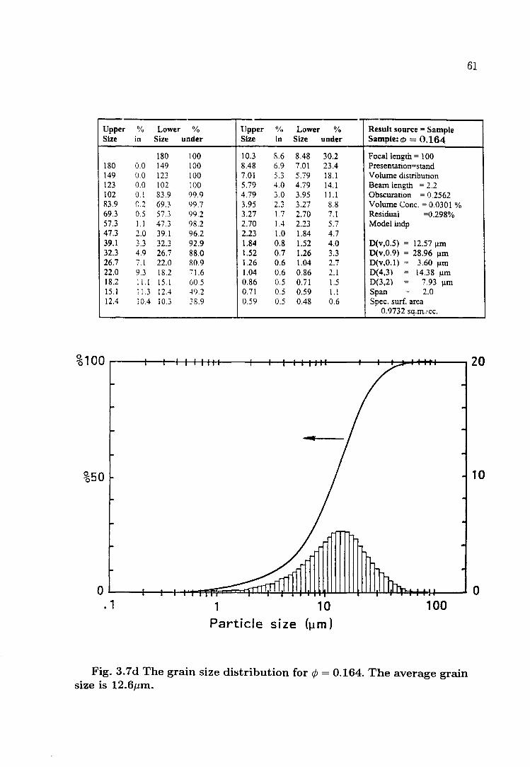
61

Upper 0/0 Lower 0/0 Upper 0/0 Lower % Result source = Sample Size in Size under Size in Size under Sample: <D = 0.164

180 100 10.3 8.6 8.48 30.2 Focal length = 100 180 0.0 149 100 8.48 6.9 7.01 23.4 Presentation=stand 149 0.0 123 100 7.01 5.3 5.79 18.1 Volume distribunon 123 0.0 102 100 5.79 4.0 4.79 14.1 Beam length = 2.2 102 0.1 83.9 99.9 4.79 3.0 3.95 11.1 Obscuranon = 0.2562 83.9 0.2 69.3 99.7 3.95 2.3 3.27 8.8 Volume Conc. = 0.0301 % 69.3 0.5 57.3 99.2 3.27 1.7 2.70 7.1 Residual =0.298% 57.3 1.1 47.3 98.2 2.70 1.4 2.23 5.7 Model indp 47.3 2.0 39.1 96.2 2.23 1.0 1.84 4.7 39.1 3.3 32.3 92.9 1.84 0.8 1.52 4.0 D(v,0.5) = 12.57 Ilm 32.3 4.9 26.7 88.0 1.52 0.7 1.26 3.3 D(v,0.9) = 28.96 Ilm 26.7 7.1 22.0 80.9 1.26 0.6 1.04 2.7 D(v,O.l) = 3.60 Ilm 22.0 9.3 18.2 71.6 1.04 0.6 0.86 2.1 0(4,3) = 14.38 Ilm 18.2 11.1 15.1 60.5 0.86 0.5 0.71 1.5 0(3,2) = 7.93 Ilm 15.1 11.3 12.4 49.2 0.71 0.5 0.59 1.1 Span = 2.0 12.4 10.4 10.3 38.9 0.59 0.5 0.48 0.6 Spec. surf. area

0.9732 sq.m./cc.

%50

O~--r-~~~~~~~~~~~~~~~~~~~ . 1 1 10 100

Particle size (~m)

Fig. 3.7d The grain size distribution for ¢ = 0.164. The average grain size is 12.6Jlm.

10

o

(a)

Scale: 122 . 05 um I I I

(b)

Scale: 122 . 05 um i I

Fig. 3.8 Optical micrographs of the grain in a powder with: (a) 1> = 0.158; (b) 1> = 0.41.

62

63

3.3 Measurements of the Conductivity and Dielec

tric Constant

3.3.1 Measurements on the Disc and Parallelepiped Samples

Axial Conductivity and Dielectric Constant Measurements

The DC resistances of the disc samples for 1> < 1>c were all measured using a

Keithley 617 electrometer in V / I mode ( two probe configuration) operated at 100V.

Because in this case the sample resistances can be as high as 5x1014 0 and the mea

surement current can go down to O.2pA, an electrical shield around both the sample

and current lead is absolutely necessary. The shielded box required for this purpose

was made in the laboratory. The insulation of the sample holder from current lead

to ground was examined by measuring the resistance of an open circuit, i.e. with no

sample between current and voltage leads. This measurement shows that the insu

lation resistance is higher than 2xl0160, which is at least 40 times larger than the

maximum resistance of the insulating discs measured. Therefore, this procedure made

resistance measurements on insulating discs reliable. A 100V DC signal was always

applied for 30minutes to allow the sample to reach equilibrium, before the reading

of the resistance was taken. For 1> > 1>c, the two-probe method was also employed,

using the Keithley 617 electrometer operating in an Ohm-meter (constant current)

mode for resistances larger than 1000. When the resistance was below lOOn, separate

voltage and current leads embedded in each of the electrodes had to be used. In these

measurements, the DC current, which was controlled by a combination of the voltage

source and buffer resistors, is in the range of 0.05 - 5mA. The voltage and current

were measured simultaneously using two digital volmeters. Good linearity was ob

tained for the range of currents used and no heating effects were observed during the

experiments.

64

The AC resistance and capacitance of the disc samples were measured in an R-C

parallel circuit mode at room temperature in the frequency range 30Hz to 100MH z

and with two equidistant points per decade on a log-scale. An ESI 2150 Video Bridge

was employed in the frequency range 30Hz to 100kHz. The bridge was always set

up to auto-average over twenty (the maximum) consecutive measurements, and was

calibrated prior to use by making open and short circuit corrections, in order to get

rid of the effects of lead resistances and stray capacitances. The bridge was operated

in either the constant voltage or constant current mode depending on the resistance

of the sample measured. For the samples with a DC resistance larger than 1000n,

a constant voltage method was used together with the standard oscillator level of

1 Vrms, in order to get good signal-to-noise ratio. A constant current, with arms

value of 1 mA, was used to measure the samples of a DC resistance less than 1000n.

In the high-frequency regime, 300kH z - 100MH z, a Hewlett-Packard (HP) 4592A

network/spectrum analyzer, with a HP45925A impedance test kit, was used. The

analyzer was operated in the impedance mode and routinely calibrated using three

standard terminations: short, open and a 50n load. The data was averaged over 300-

500 readings to reject random noise. In both the low- and high-frequency regimes,

care was taken to ensure that the levels of signal used did not cause heating. The

conductivity and dielectric constant were derived from the equivalent parallel resis

tance and capacitance readings given out by the instruments.

Transverse DC Conductivity Measurements

The measurements of DC conductivity of the conducting parallelepiped samples

(4) > 4>c only) were carried out using a conventional four-lead geometry. The voltage

across the two voltage leads and current flowing through the sample were measured

directly and simultaneously using two digital volmeters.

Because of an unsuitable geometry (i.e. a small cross-section area (8x2mm) rela-

65

tive to a larger length (24mm)), measurements of the AC resistance and capacitance

for insulating parallelepiped samples "were not feasihle or unreliable, and consequently

are not included in this work.

3.3.2 Measurements on the Powder Samples

It was probably the equal densities of graphite and hexagonal boron-nitride that

made the powder experiments possible since there is no relative precipitation between

the graphite and boron-nitride powders during powder pouring and while they are

being compressed. Any humidity inside the powder can lead to a large spurious

conductivity, as the BN component has a very high resistivity. Therefore all the

powder experiments, including the pouring and the electrical measurements, had to

be performed in an air-conditioned room with a relative humidity of less than 12%

at room temperature. To check for inconsistencies, each powder experiment was

repeated three times.

Measurements in the Axial Direction

The axial DC conductivities of 50%G-50%BN and 55%G-45%BN powders were

measured in a polyethylene cylindrical vessel of 42mm internal diameter with a smooth

brass bottom, which together with a close fitting non-rotating brass plunger formed

the electrodes. The vessel and the plastic framework, which supported the plunger,

were mounted on a plastic base. The plunger could be moved downwards using a

0.5mm pitch precision thread mechanism, which was calibrated before performing

the experiments. This measurement system is very similar to that used to measure

the axial AC conductivity and dielectric constant (see Fig. 3.9). The resistance of

the empty vessel is above 2xlO16!1, which is over 50 times larger than the maximum

resistance of any powder measured.

To have a very low and constant initial apparent powder density in the vessel,

special pouring methods had to be used. The plunger, together with the plastic

66

framework supporting it, was first removed. The powder was first poured into a

cylind~r with a sieve bottor.1, which was placed over and coverin6 the orifice of the

sample vessel. A solid bar, of the same length as the internal diameter of the cylindri

cal sieve and resting on the sieve bottom, was slowly rotated around a central pivot

to agitate the powder, causing it to fall slowly through the sieve into the vessel. After

this procedure, the plunger and the plastic framework were put back in the position,

as illustrated in Fig. 3.9, and the whole system was then placed in an electrically

shielded metal box. The voltage and shielded current leads from the electrometer

were connected to the electrodes of the powder cell. To increase the volume fraction

of graphite, the plunger was moved down gradually, and the corresponding volume

fraction was calculated from the weight and density of the graphite in the powder and

the total volume between the bottom plate and the plunger, whose position relative to

the bottom plate is accurately known at all times from the micrometer or calibrated

thread position. Near the percolation threshold the volume fraction increments were

very small, 0.001 (0.1%). The following formula was used in the graphite volume

fraction calculations for a cylindrical vessel in the powder experiments:

Here

M· wp·!' 4> = p

h . 7rr2

wp = 4.955 x hr2 '

M = the mass of powder mixture, 35.00±0.01grams;

(3.3)

wp= 0.50 for the 50%G-50%BN powder and 0.55 for the 55%G-45%BN powder;

p= the density of the graphite or boron-nitride, 2.259/ em3;

h= the separation between the bottom plate and plunger, em;

r= the internal radius of the cylindrical vessel, em.

At the beginning of an experiment the apparent density was about 0.369/ em3

which corresponds to a packing fraction for the G-BN powder of about 0.16. The

67

downward motion of the plunger was limited by the torque that could safely be ap

plied to the calibrated thread. Th,~ resulting maximum apparent density was about

0.639 I cm3 and packing fraction of about 0.28. This packing fractions mean that there

were always cavities in these powders during the measurements.

The DC resistance was measured using the Keithley 617 electrometer in the VI I mode. A voltage of 100V was used for resistances larger than 200CO and the voltage

was lowered to 10V and then down to 0.5V, as the powder became more conductive

with increasing graphite volume fraction while the plunger was moved down. The

minimum resistance of powder in these experiments was larger than 1000 due to the

limitation of maximum torque which can be safely applied to the plastic framework

and the thread. After the resistance had been read for a particular volume fraction,

the Keithley electrometer was set to the zero check state, and then the plunger was

slowly advanced to the next volume fraction position. After a pause of 5minutes to let

the grains settle down, the zero check state was removed and the resistance recorded,

after the reading had become stable. This usually took 15mins on insulating side and

less than 1min on conducting side. Resistances between 200CO and 20CO, where

<P ~ <Pc, were too unstable to be measured.

Because the powder experiments gave extraordinary high values of the exponent

t, a second pouring method had to be developed to check if the pouring procedure

played a role. For this second method, a close fitting perspex piston, with a 1cm slot

in the middle, was placed in the cylindrical cells. The slot was then filled and kept

full of powder as the piston was moved upwards, with a rotating action, using a 1mm

pitch threaded rod, and the powder was stroked into position with a "twist" motion.

Fig. 3.9 shows the system used to measure the axial AC conductivity and dielec

tric constant. In this case the cylindrical capacitive vessel consisted of a glass wall of

70mm internal diameter, a close fitting non-rotating plunger and the bottom plate.

The plunger and the bottom plate, which were made from circuit boards backed by

polyethylene plates, formed the two capacitor plates. The plunger was moved down

glass tube --+-1.."1

polyethelene plate --+-N?'

copper layers

perspex plate

micrometer

- metal

sample power

teflon rod

s pect .. n''nD,r Dr"

circuit board plates

Fig. 3.9 Schematic diagram of the system used to measure the axial AC electrical conductivity and dielectric constant for powders.

68

69

using a 25mm micrometer head. The methods of pouring the powder into the ves

sel were the same as de~cribed above and the similar sieves with the appropriate

diameters were used. An ESI 2150 bridge (30Hz - 100kHz) and a HP4592A net

work/spectrum analyzer with HP45925A impedance test kit (300kHz - lOMH z)

were used to measure the AC resistance and capacitance in the parallel circuit mode

at room temperature. The calibration and set up of these two instruments are ex

actly the same as those for measuring the discs described in the previous subsection.

Whenever the volume fraction was changed, the leads of either the ESI bridge or the

impedance test kit were first disconnected from the sample vessel. Then the plunger

and the bottom plate were electrically shorted out and the plunger was moved to

a new volume fraction position. After a few minutes pause, the short circuit was

removed and the four leads of the ESI bridge were reconnected to the vessel for low

frequency measurements. The leads of the ESI were then replaced by two leads of

HP45925A for the high frequency measurements. In this experiment, the leads were

kept as short as possible, and great care was taken to ensure that the leads of the

instruments were always in the same configuration when performing the measurement

as they had been during the calibration procedure.

Measurements in the Transverse Direction

The apparatus and methods used to measure the transverse resistances and capac

itances of the powders are very similar to those used for axial direction measurements.

Therefore only the major differences in the design of the sample cells are described

below.

The DC Measurements

To keep the stress distribution within the powder as close to that in the axial

measurements as possible, the "powder cell " of the measurement system for the

transverse DC conductivity was designed to be nearly the same as that used for axial

measurements. The principal differences are that the walls of the cylindrical vessel

70

now consist of two 90° brass sectors separated by two 90° polyethylene sectors, and

the plunger and bottom of the vessel are both polyethylene. In this case, the geomet

ric factor, which is used to derive the conductivity from the resistance data, could

not be calculated in a straightforward manner, and was therefore determined exper

imentally by painting 90° silver electrodes on the sides of 42mm diameter graphite

cylinders of known resistivity and different lengths.

The AC Measurements

In this case the sample cell had to have a parallelepiped shape, with fixed thick

ness and variable cross-sectional area. Two 170x115mm copper/fibre glass circuit

boards, with 150xl15mm copper sheet in the middle, formed the two capacitance

plates. These two circuit boards, backed by polyethylene sheet, were separated by

two 10xlOx115mm polyethylene spacers, and screwed to a polyethylene base. The

plunger was a close fitting polyethylene section with a cross-section of 10x150mm,

and was driven downwards by the same 0.5mm pitch precision screw as used in the

axial DC measurements. The capacitance of the empty cell was calibrated against

plunger height, so that the capacitance between the area of the capacitor plates cov

ered by the plunger could be corrected for. A slot shaped sieve was used to pour the

powders and a soft brush was moved backwards and forwards in the sieve to get the

powder to flow through the mesh and into the cell.

3.4 Measurements of the Magnetoresistance and

Hall Coefficient

The magnetoresistances of the conducting G-BN parallelepipeds near the perco

lation threshold were measured at room temperature in magnetic fields up to 1.5T.

Fig. 3.10 shows a block diagram of the electric circuits and instruments used for

automated measurements of the magnetoresistance and Hall coefficient. The data

acquisition program is an analogue to the so-called DIP system, which is used to

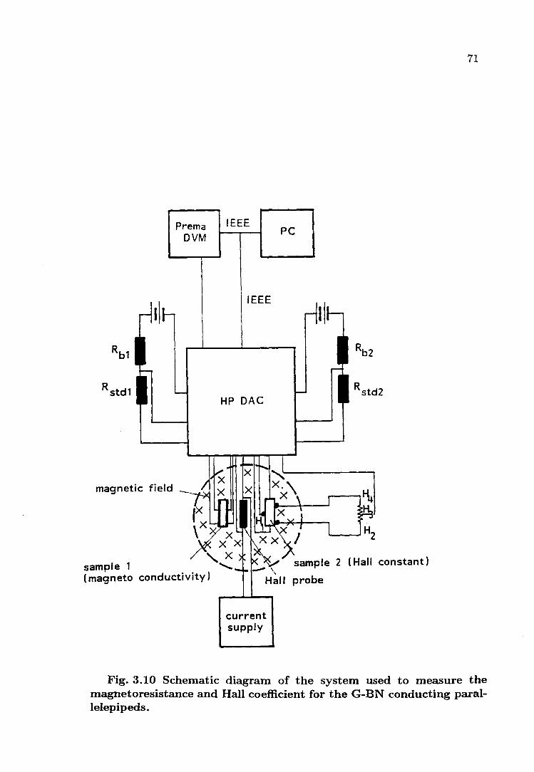
RStd1

magnetic field

Prema DVM

sample 1 (magneto conductivity)

IEEE PC

IEEE

HP DAC

Hall

current supply

71

Rstd2

2 (Hall constant)

Fig. 3.10 Schematic diagram of the system used to measure the magnetoresistance and Hall coefficient for the G-BN conducting parallelepipeds.

72

measure the temperature dependence of various resistances in a range 1.8 - 300K,

and was fully describecl by Albers (1994). The one major difference is that the Hall

probe reading replaced the thermometer reading and the magnetic field replaced the

temperature.

The desired currents through each sample were obtained by choosing appropriate

values of the buffer resistors RbI and Rb2 (see Fig. 3.10). The polarity and magni

tude of the magnetic field was controlled manually by reversing and varying the DC

current in the windings of the magnet. A relay in the HP DAC (a HP3497 A Data

Acquisition/Control Unit) was used to reverse the direction of the sample current

at every data point. The resistance of the sample was determined from the voltages

across the sample and across the standard resistor. In order to cancel the spurious

voltage due to misalignment and thermomagnetic effects, the average was taken for

four readings: two by reversing the directions of the current and a further two by

changing the polarity of the magnetic field. The HP DAC connected in turn the Hall

probe leads and the many other voltage leads to the Prema 5000 Digital Voltmeter

(DVM). When the circuit, which was being connected to DVM, is stable, the read-out

digital signal from DVM is transferred to the PC for data reduction.

Several other salient features of this measurement system are described below.

The sample geometry

The length-to-width ratio of a rectangular parallelepiped sample influences the

measured magnetoresistance and Hall coefficient in opposite ways [Putley 1960, Chap

ter 2]. Here the length is defined along the edge of sample with the same direction of

the current, while the width is along the edge perpendicular to both the directions

of the current and magnetic field. For the Hall coefficient, if the Hall voltage is mea

sured on a short wide sample, with large area current electrodes at each end, then

the voltage measured would be less than that expected from the simple theoretical

expression. The reason for this is that the current electrodes at the ends tend to

short out the Hall field. Quantitative calculations have shown that to eliminate this

shorting effect the length-to-width ratio must be greater than 3 or 4. On the other

hand, the Hall electric field ')ends to prevent the curva.ture of the mean free path in

the presence of a magnetic field, which is responsible for the increase in resistance.

Therefore if the Hall field is shorted out, the measurement of the resistance change

due to magnetic field will be more accurate. Therefore, while a large length-to-width

ratio ( ~ 3 ) is recommended for Hall effect measurements, a much smaller ratio is

better for measuring the magnetoresistance.

Because of this, two different sample geometries were used to measure the magne

toresistance and Hall constant in the present study. For the magnetoresistance, the

parallelepiped samples with a length-to-width ratio of 1/6 were chosen in order to get

a larger differential voltage signal due to an external magnetic field. Since the length

of the sample is now too short to allow two voltage leads to be connected on its edge,

a quasi-four probe method has to be employed to measure the magnetoresistance.

For the Hall coefficient, parallelepipeds with length-to-width ratio of 3, which

were also used to measure the transverse conductivity, 1/ f noise and thermoelectric

power, were selected. As shown in Fig. 3.10, one Hall contact HI was applied at the

geometrical middle point on one side of sample along the direction of the current,

and on the another side a IMf! (low noise) metal film potential divider H2H3H4 was

connected. With the magnet off, the position of the wiper (H3) was adjusted to give

zero potential difference between HI and H3. With this circuit, when the magnet is

switched on, the Hall voltage should appear between HI and H3.

The Hall probe

A Siemens SBV538 Hall probe, driven by a 30mA DC current, was used to mea

sure the magnetic field. It was calibrated at room temperature against the NMR

(Nuclear Magnetic Resonance) Gaussmeter in the EPR laboratory of the physics de

partment. The Hall voltage from the probe was measured during the experiment and

converted to the magnetic field magnitude using the calibration data.

74

The magnet

A commercial electric-magnet (Newport Instruments), with conical pole pieces of

145mm initial and 70mm final pole diameters, was used to generate the magnetic

field which ranged from OT to 1.5T. Tapwater flowed though the cooling tubes in the

coils. Two HP6528A DC power sources were connected in a master-slave mode to

supply the current to the magnet. The direction of the magnetic field was reversed

by changing the direction of the coil current, at nearly zero current, using a reversing

switch.

The sample and Hall probe holder (not shown in Fig. 3.10)

The two samples to be measured were mounted on a flat polyethylene base, while

the Hall probe was mounted on the underside of the base. The polyethylene base was

supported by a wooden frame on the side of the magnet and adjusted to be parallel to

the pole surfaces. Since the samples were held flat on the surface of the polyethylene

base, the magnetic field and the direction of sample current were always vertical to

each other during the measurements.

Because no Hall voltage signal could be detected at room temperature using the

measurement system described above, measurements were also made at liquid ni

trogen temperature, as the Hall coefficient for pure graphite increases rapidly with

decreasing temperature. In the low temperature experiment, the sample was mounted

on a teflon bar inserted in a stainless steel tube. This tube was then placed in a glass

dewar of 17mm inter diameter, filling with liquid nitrogen, and the dewar was clasped

vertically in magnetic field. At liquid nitrogen temperature, in addition to the DC

method shown in Fig. 3.9 and discussed above, an AC method using a lock-in am

plifier, operated at a low frequency, was also used to try to detect the Hall voltages.

Unfortunately no Hall voltage was detected at liquid nitrogen temperature, using

either the DC or the AC method. Because of the time limitations for this project,

75

further improvements of the Hall measurement system could not be carried out.

3.5 1/ f Noise Measurements

The 1/ f noise experiments were carried out on conducting discs and parallelepipeds,

near the percolation threshold. The measurements can be classified into two types

according to their final objective: first, to measure the power-law for the normal

ized noise power against the sample resistances; second, to measure the sample size

dependence of the normalized noise power for the samples near the critical volume

fraction, where the fractal structure of the infinite cluster could dominate the physical

properties of the sample.

The 1/ f noise measurements were all made at room temperature over the fre

quency range 1Hz - lOOOH z. A number of fresh 9V alkaline batteries connected in

series formed the DC voltage source. A wire wound buffer resistor, or buffer resistors

in series, with at least ten times the sample DC resistance, was connected in series

with the sample to be measured. The voltage drop across the sample was amplified

by a Stanford Applied Research SR560 Preamplifier, with the bandpass filter set at

O.3H z and 3kHz in the low noise mode and running on its internal rechargeable

batteries. The alkaline batteries, sample, buffer resistor(s), and preamplifier were all

placed inside a grounded steel box. The output of the preamplifier was transmitted

to a HP3562A signal/spectrum analyzer, which performs the analogue Fast-Fourier

Transform (FFT) to give a noise power spectrum. A PC computer, connected to

HP3562A through the IEEE bus line, recorded and plotted the spectrum. The DC

current through the sample was varied by changing either the number of batteries in

series or the resistance of the wire wound buffer resistor( s). The background noise

from the batteries and preamplifier was examined by measuring the noise generated

by a wire wound resistor, which replaced the sample in the circuit and had approxi

mately the same resistance. This measured background noise is about four orders of

magnitude smaller than the smallest 1/ f noise level measured for the samples. The

76

contribution of the noise from the contacts between the sample and the electrical leads

to the measured 1/ f noise was also found to be negligible in these experiments. This

conclusion was made because when one doubled the resistance of the buffer resistor

and the voltage of the DC source (therefore the current through the sample is the

same but the ratio of buffer resistance to sample resistance was doubled), no change

in the slope and the magnitude of the noise power spectrum was observed [Leeman

et al. 1980].

The 1/ f noise spectrum between 1Hz and 1000H z was taken for each sample and

averaged for between 300 to 1000 sweeps by the signal analyzer. The background or

thermal noise (i.e. zero current noise), which superposed on the 1/ f noise spectrum

generated by the current, was recorded first and later subtracted from the 1/ f noise

spectrum. In order to verify the /2 or V2-dependence of the 1/ f noise spectrum,

six or seven selected DC currents were used for each sample. The DC resistance

of sample was also measured with the same electrical lead configuration, and using

the same six or seven DC currents as that for the 1/ f noise measurements. The re

sults of these resistance measurements showed that the noise measurements were all

taken within the Ohmic regime of the samples, and no heating effect was taking place.

The experiment to investigate the sample size dependence of the normalized 1/ f noise power was performed in the following way. Disc shaped samples with a graphite

volume fraction 4> in the range 0.154 - 0.175 were made and selected. These discs

were first cut into the largest rectangular shape possible and the 1/ f noise was mea

sured, in the transverse direction. Several DC currents were used to check the ]2_

dependence of the noise power and the linearity of the resistance. Next, while keeping

the sample thickness constant, the length and width were cut down so as to keep an

approximately constant length-to-width ratio. The noise and resistance were mea

sured in the same way as before, and then the size of the sample was reduced again.

The series of sizes for two typical samples are given below:

</> = 0.1537 : (1) 2.78x15.9x16.4mm, (2) 2.78x12.8x13.9mm, (3) 2.78x9.90x11.1mm, (4) 2.78x7.70x8.60mm, (5) 2.78x3.50x3.90mm.

</> = 0.1785 : (1) 2.20x18.1x18.1mm, (2) 2.20x16.3x16.3mm, (3) 2.20x14.6x14.6mm, (4) 2.20x12.3x12.3mm, (5) 2.20x10.2x10.2mm, (6) 2.20x8.40x8.40mm, (7) 2.20x6.20x6.20mm.

3.6 Measurements of the Thermoelectric Power

77

The thermoelectric power measurements were made on conducting parallelepiped

samples with graphite volume fractions from 0.154 to 0.82. The temperatures of the

hot and cold ends of the sample to be measured were controlled so as to be 5±0.2°C

and 45±0.2°C respectively. The apparatus, which was placed in an evaporation plant,

is shown in Fig. 3.11. Two 50x60x 1 Omm copper blocks formed the heat sink (cold

block) and heat source (hot block) respectively. A heater coil was wound onto the

hot block, which was thermally and electrically insulated from the copper base plate

by four nylon screws. The heat sink is thermally and electrically connected to the

copper base plate through two copper screws. The base plate was thermally coupled

(welded) to the copper tube, through which the chilled cooling water passed. Two

calibrated PTlOO thermometers were embedded in each copper block to measure the

temperatures. A standard four-probe method was employed to measure the resis

tances of these two thermometers. A constant current of 1mA from two Lakeshore

123 current sources passed through each thermometer. The voltage drops across the

two thermometers were monitored continuously by two digital voltmeters. The volt

age drop across the PTIOO in the hot copper block and the 1mA current signal were

simultaneously fed to the temperature sensor of a homemade PTe (positive temper

ature coefficient) temperature controller. The output of the temperature controller

was fed to the heater coil on the hot block, which provided the power necessary to

control the temperature of the hot block.

Silver paste was painted on the two 8x2mm ends of parallelepiped sample. The

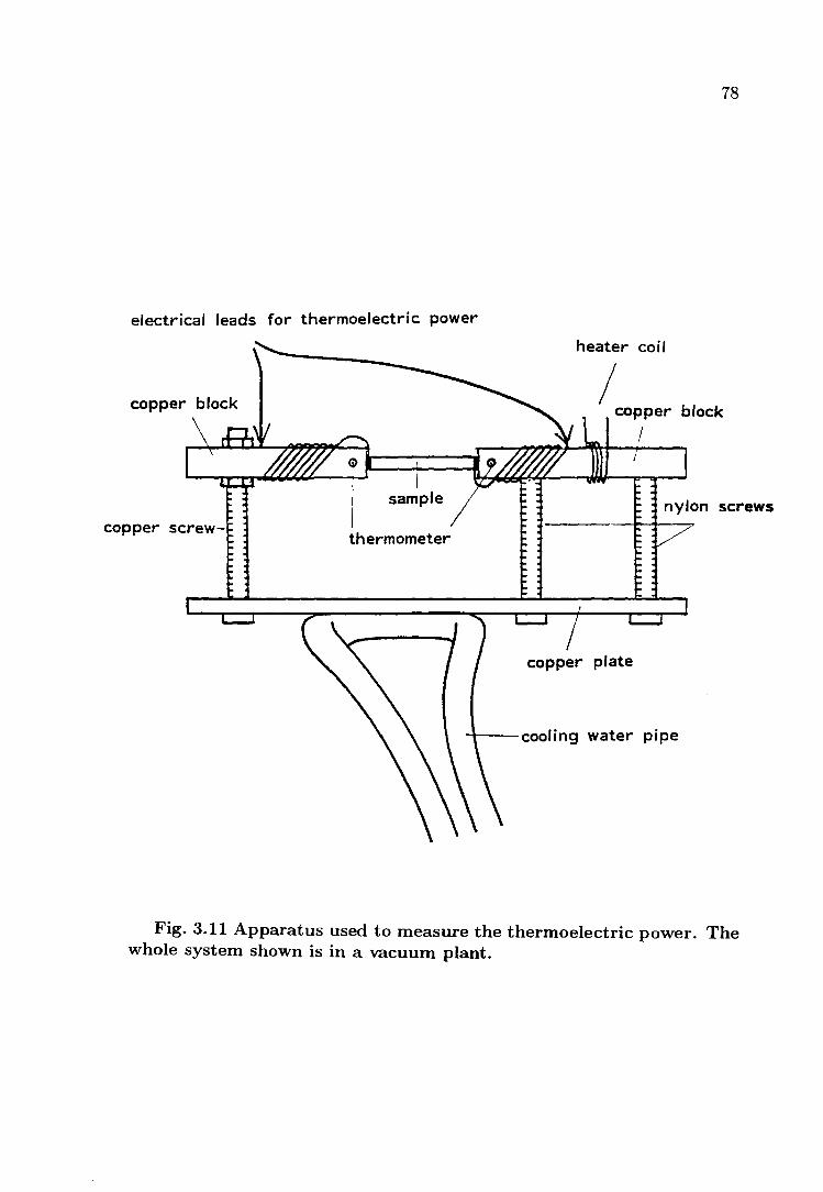
78

electrical leads for thermoelectric power

heater coil

copper block / copper block

I

I sample

thermometer

4---cooling water pipe

Fig. 3.11 Apparatus used to measure the thermoelectric power. The whole system shown is in a vacuum plant.

79

sample was then mounted, with the silver paint still wet, between the two copper

blocks, after two electrical leads (copper wires) had been embedded in silver paint ..

These leads, between the sample and each copper block, were used to measure the

electrical potential difference. In order to avoid unwanted heat gradients, all the

electrical leads, including all the leads for the two thermometers, were heat sunk by

winding several turns of each wire around the corresponding copper blocks. A Prema

5000 6i digital voltmeter with resolution of O.II1V was used to measure the voltage

between the cold and hot ends of sample. During the experiment, iced water was

pumped through the cooling tube which cooled the heat sink (cold block) down to

5±0.2°C, while the hot copper block was warmed up to 45±0.2°C by the temperature

controller and heater. Inside the belljar the pressure was less than l.OxIO-sTorr. The

potential difference between the two ends of the sample being measured was read

from the DVM, when the temperatures of two PTIOO thermometers had been stable

for about half an hour. It should be noted that in the temperature range from 5°C

to 45°C there is no thermodynamic phase transition in the G-BN samples, so that a

constant thermoelectric power is a reasonably good approximation for these samples.

This was later confirmed in the experiments since approximately the same thermo

electric power data was obtained when the temperature of the hot end of sample was

set-up in the range 10° - 45°C, but a larger temperature difference was preferred as

it gave more accurate voltage readings on the DVM.

Before performing the measurements on the samples, the entire system was cali

brated by soldering a constantan wire between the two copper wires wound onto both

the cold and the hot copper blocks, and making measurements under the same condi

tions as the sample experienced during the experiment. The thermoelectric power of

copper-constantan thermocouple measured in this system was 38.411 V /K, reasonably

close to the generally accepted value 40.211 V /K.

80

3.7 Data Fitting Technique

The least squares fitting program of a commercial software package "Microsci

entist" was used to fit the relevant percolation equations to the experimental data

obtained for the G-BN samples. A statistical program in the package gave the stan

dard deviation with 95% confidence for each estimated parameter. For a parameter,

which was obtained from fitting the experimental data from different runs, a weighted

average was taken over all the estimated values in the following way

(3.4)

where "ii is the best final estimation of parameter a, "iij is a least squares fitting of the

data obtained from the j-th run, and OJ is the corresponding standard deviation. 0*,

the standard deviation given for "ii, is obtained from

0* = --==1== JLj~·

(3.5)

The critical volume fraction <Pc is the most fundamental parameter used to de

scribe a particular percolation system, as it explicitly appears in all the expressions

involving various critical exponents. The following method was used for fitting the

data to obtain the best values for <Pc and the critical exponents.

First, <Pc and conductivity exponents t and s were obtained by simultaneously fit

ting the two percolation equations for DC conductivity on each side of the percolation

transition to the DC conductivity data. In this step, <Pc, the two pre-factors and the

two exponents t and s, were treated as free parameters and were determined as the

values for which a minimum residual was obtained.

Secondly, the <Pc value obtained in step one was fixed, the pre-factor and the expo

nent in the relevant percolation equations, other than those for the DC conductivity,

were allowed to vary. An estimation of the pre-factor and the exponent and their

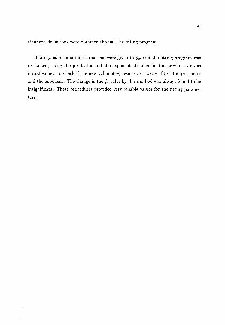
81

standard deviations were obtained through the fitting program.

Thirdly, some small perturbations were given to <Pc, and the fitting program was

re-started, using the pre-factor and the exponent obtained in the previous step as

initial values, to check if the new value of <Pc results in a better fit of the pre-factor

and the exponent. The change in the <Pc value by this method was always found to be

insignificant. These procedures provided very reliable values for the fitting parame

ters.

Chapter 4

THE ELECTRICAL

CONDUCTIVITY, DIELECTRIC

CONSTANT AND

MAGNETORESISTANCE

4.1 Introduction

82

As previously stated, the electrical conductivity and dielectric constant of random

metal-insulator mixtures are the most widely investigated physical properties in per

colation studies. Like other second order phase transitions, metal-insulator transitions

are observed by a steep change of electrical conductivity in a narrow range of metal

volume fractions. As already discussed in Chapter two, scaling theory predicts that,

near the percolation threshold <Pc, the DC conductivity follows the power-laws (2.19)

and (2.20) and that the low frequency dielectric constant follows another power-law

(2.23). It also predicts that the AC conductivity and dielectric constant scale with

frequency as described by (2.29), (2.30) and (2.31). Two physical models, namely

intercluster polarization and anomalous diffusion, have been suggested to explain the

AC scaling behaviour. They give rise to different expressions for the exponents x and

y in (2.27) and (2.28), and (2.36) and (2.37) respectively.

83

The experimental dcta for the DC conductivity and the real part of the low fre

quency dielectric constant obtained from the disc samples, and the 50%G-50%BN and

55%G-45%BN powders are presented and analyzed in Section 4.2. The experimen

tal results for the complex AC conductivity measurements are given and discussed

in Section 4.3. The measured relative magnetoresistivity and magnetoconductivity

are presented in Section 4.4. The chapter ends with a summary of the finding and

discussions in Section 4.5.

In this chapter, the vacuum permittivity Co is left out in both c(</>,O) and c(</>,w),

i.e. they are relative dielectric constant, in contrast to that used in Chapter 2.

4.2 The DC Conductivity and Low Frequency Di

electric Constant

The axial DC conductivity was measured for two sets of disc samples below and

above the percolation thresholds, while the transverse DC conductivity was measured

only on parallelepipeds cut from the second set of disc samples on the conducting side.

Except where otherwise stated hereafter, the disc and parallelepiped samples referred

to are the second set. For the 50%G-50BN and 55%G-45%BN powders, the mea

surements of the axial and transverse DC conductivities were made, using different

cells, as described in Subsection 3.3.2. All the low frequency dielectric constants were

measured at lOOH z and 1000Hz.

In this section, the experimental results on the DC conductivity and the real part

of the low frequency dielectric constant for G-BN disc samples and powders are pre

sented. The discussion and comparison with other previously published experimental

results are given, usually by a comparison of the critical volume fraction </>c and the

critical exponents t, sand s.

84

4.2.1 Results

Fig. 4.1 shows the logarithm of the room-temperature axial DC conductivities

0"( <p, 0) as a function of the volume fractions for the second set of disc samples and

a typical run on 55%G-45%BN powder. Both the conductivities vary by more than

14 orders of magnitude over the range of 0:;:; <P :;:; 0.23, with a relatively small scat

ter of the data near the critical volume fraction. The crossover or critical region, 1 1

defined by (O"i/O"c)t+-; '" (10-16/102 )t+"', is too small to observe. Similar results have

been obtained for the first set of disc samples and other runs on the 55%G-45%BN

and 50%G-50%BN powders. The two percolation equations, (2.19) and (2.20) with a

common <Pc, are fitted simultaneously to the axial DC conductivity data for the discs.

This fit gives a small uncertainty in and equally good statistical properties of the es

timated parameters on both sides of the percolation threshold. The data and best fit

results are shown in Figs. 4.2a and b, where both fits use the same value of <Pc(0.150).

The transverse DC conductivity data, obtained from the parallelepiped samples cut

from the disc samples with <Pc, together with its best fit line (<Pc = 0.150), are also

given in Fig. 4.2a. Fig. 4.2c shows axial dielectric constant data for the discs, where

the solid line is a least squares fit of the power-law relationship of (2.23) to both the

lOOH z and lOOOH z data. In this fit <Pc was fixed at the value of 0.150, obtained from

the best fit of the disc DC conductivity data plotted in Figs. 4.2a and b. The pa

rameters <Pc, t, sand s for the disc samples are summarized in Table 4.1. Transverse

DC conductivity and dielectric measurements on the parallelepiped samples on the

insulating side were not possible due to unsuitable geometric factor. The capacitive

measurements on the samples well above <Pc could not be made because of the high

conductances of the samples and the limitation of the instruments used.

The conductivity data for all the discs from <p = 0 to <p=0.82 is plotted as a function

of volume fraction on a semi-log scale in Fig. 4.3. The theoretical curve in this case

is a best fit to the GEM equation and the parameters are <Pc=0.150±0.002, log O"i=-

15.86±0.04, log O"c=1.89±0.02, s=1.05±0.18 and t=3.03±0.07. These parameters are

very close to those (Table 4.1) obtained using a simultaneous fit to the two percola-

..I .-E u

I

c: -.-a

-5

o-55%G-45%BN Powder V-Disc-Shaped Samples a:P v v

00 v o v

8 v o o o

o

v

85

v v

-e--- -10 b

-15

o

v o~vv

v

v v

0.05 0.10 0.15 0.20

VOLUME FRACTION 

0.25

Fig. 4.1 The axial DC conductivity 0"(4),0) versus the volume fractions on semi-log scale for disc shaped samples and a typical run on 55%G-

45 %BN powder.

~ I .-E (.) , c: --.-a -~ --b C) 0 ...J

86

-2

-4

'V-Transverse o-Axial

-6

-8L-~~~----~~----~~~~~~~~--~

-2.5 -2.0 -1.5 -1.0

LOG(<j>-0.150)

Fig. 4.2a The axial and transverse DC conductivities against ( <Pc· The critical volume fraction is found to be mc=O.150 ±O.OOl, and the values of t exponent are t = 2.63±O.07 and 2.68±O.13 in the axial and transverse directions respectively.

...... I .-. E u

I

C --.-. a --e---b (9 0 .....I

87

-14.5

-15.0

-15.5

-16.0 ,--",----,---,"---o......-JI.....-....o----,----,---,---....JI.....-....o----,----,--o---'--o----o.----l:....-...--.....J

-2.5 -2.0 -1.5

LOG(0.150-<t»

-1.0 -0.5

Fig. 4.2b The axial DC conductivity against (cPc-cP) for cP < 1Jc, where CPr =0.150. The value of s is found to be 1.01±0.05.

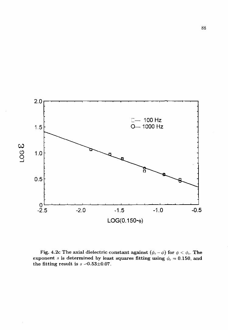
1.5

w

0- 100 Hz 0-1000 Hz

88

8 1.0 ....J

0.5

O~~~~~--~~~~~--~~~~~--~~~~~~

-2.5 -2.0 -1.5

LOG(O.150-q,)

-1.0 -0.5

Fig. 4.2c The axial dielectric constant against (¢c - ¢) for ¢ < c/Jc. The exponent s is determined by least squares fitting using ¢c = 0.150, and the fitting result is s =0.53±0.07.

89

Table 4.1 The observed critical volume fraction cPc and exponents s, sand t.

SAMPLE cPc s s t Discs

Axial AC 0.150 ± 0.001 0.53 ± 0.07 Axial DC 0.150 ± 0.001 1.01 ± 0.05 2.63 ± 0.07

Transverse DC 0.150 ± 0.001 2.68 ± 0.13

Axial AC 0.153 ± 0.001 0.40 ± 0.02 Axial DC 0.153 ± 0.001 1.06 ± 0.04 2.90 ± 0.20

'Poured Powder' 50%G

Axial AC 0.114 ± 0.001 0.60 ± 0.01 Axial DC 0.120 ± 0.001 0.42 ± 0.01 4.85 ± 0.46

Transverse AC 0.108 ± 0.002 0.91 ± 0.02 Transverse DC 0.116 ± 0.003 0.26 ± 0.05 6.10 ± 0.16

55%G Axial AC 0.124 ± 0.001 0.72 ± 0.01 Axial DC 0.123 ± 0.001 0.47 ± 0.01 4.80 ± 0.14

Transverse AC 0.109 ± 0.001 0.83 ± 0.06 Transverse DC 0.124 ± 0.001 0.46 ± 0.01 6.06 ± 0.13

'Twist' Powder 50%G

Axial AC 0.127 ± 0.001 0.53 ± 0.01 Axial DC 0.123 ± 0.001 0.93 ± 0.13 4.64 ± 0.04

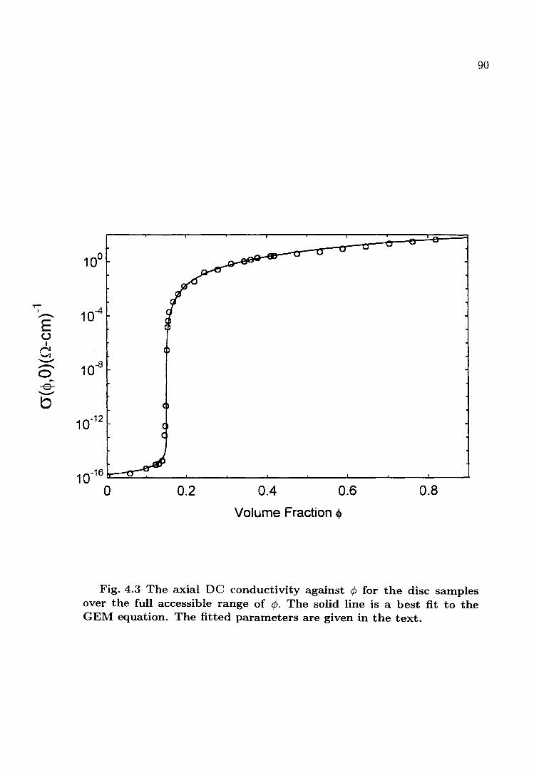
..-I .-E (,)

I c: --.-0 -e---b

90

10-4

10-8

10-12

10-16~~~----~--~----~--~----~--~----~--~ o 0.2 0.4 0.6 0.8

Volume Fraction cjl

Fig. 4.3 The axial DC conductivity against ¢ for the disc samples over the full accessible range of ¢. The solid line is a best fit to the GEM equation. The fitted parameters are given in the text.

91

tion equations, to the data in the volume fraction range from < 0.24 the GEM equation gives <Pc=0.150±0.002, logO"i=15.86±0.0l,

log O"c=1.50±0.13, s=1.05±0.04 and t=2.7±0.24 in excellent agreement with the val

ues given in Table 4.1.

Using <Pc = 0.150, Equation (2.19) is also fitted to the axial disc conductivity

data in the range 0.150<<p<0.82, as shown in Fig. 4.4. In this case, the conductivity

exponent t is found to be 2.74, consistent with the value obtained from the data over

the narrower volume fraction range 0.150 '" 0.240. Similar observations, that the

percolation equations can, in some cases, fit the DC conductivity data over a wide

range of volume fractions, were also noted by many authors [McLachlan 1986 and

Kolek and Kusy 1991, and references therein].

The parameters <Pc, t and s for the axial and transverse DC powder conductivity

data, on both sides of the metal-insulator transition, were also obtained using simul

taneous fits of the data to Equations (2.19) and (2.20). Again due to the limitation

of the instruments, the axial and transverse dielectric constant data at lOOH z and

1000H z could be obtained for <P :::; <Pc only. Therefore in this case both <Pc and shad

to be treated as fitting parameters. Figs. 4.5a, b, and c show the data and fitted

results for a typical run of powder experiments. The parameters <Pc, t, sand s ob

tained by fitting the experimental data were averaged over three runs of the powder

experiments, and the results are summarized in Table 4.1. It is seen from the table

that the values of <Pc for the transverse capacitive measurements are somewhat lower

than those for the axial. This is attributed to the very different geometry of the two

capacitive cells used. The dielectric exponent s, found at 100Hz and 1000Hz, are

virtually equal.

4.2.2 Discussion

The critical volume fractions

The observed critical volume fractions for the two sets of discs of 0.150±0.00l

..-I ...-E u

I c: --...-a --e---b (9 0 .....J

0

-2.5

-5.0

-7.5

Fig. 4.4 The axial DC conductivity for the conducting disc samples against (rP - rPc) over the full accessible range of rP, where rPc= 0.150. The solid line is a least squares fit to the data, which yields t=2. 74.

92

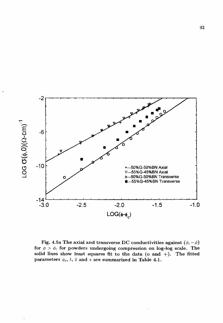
~ I ..-E u

I

c: -..-a -e---b (9 o .....J

-6

-10 +-SO%G-SO%BN Axial V-SS%G-4S%BN Axial o--SO%G-SO%BN Transverse .-5S%G-4S%BN Transverse

-14~~~~~~~~~~--~~~~~~~~~~~

-3.0 -2.5 -2.0

LOG(cI»-cI» ) c

-1.5 -1.0

Fig. 4.5a The axial and transverse DC conductivities against (cPc - cP) for cP > cPc for powders undergoing compression on log-log scale. The solid lines show least squares fit to the data (0 and +). The fitted parameters CPo t, sand s are summarized in Table 4.1.

93

..-I .-E C,.)

I c: --.-a -Er --b (9 0 .....J

94

-14.0

V-55%G-45%BN Axial o-50%G-50%BN Axial

-14.5 v v l&- v --s- __ V ,... ,.. v v v V

-15.0 - .

~ .-55%G-45%BN Transverse

-15.5 +-50%G-50%BN Transverse r--. - - --+ -

-16.0 r + + + + -+ + + + +-

-16.5 -2.8 -2.4 -2.0 -1.6

LOG(cpc-cp)

Fig. 4.5b The axial and transverse DC conductivities against (cPr - ¢) for ¢ < ¢c. The CPr values used are the same as those used in Fig. 4.5a.

w (9 o .....J

1.3

1.1

0.9

0.7

v-55%G-45%BN Axial o-50%G-50%BN Axial +-55%G-45%BN Transverse .-50%G-50%BN Transverse

0.5L-~~--~~~--~~~--~~~~~~~~~

95

-2.5 -2.0 -1.5 -1.0

Fig. 4.5c The axial and transverse dielectric constants against (cPc-cP) for dJ < cPc· The (jJ, values used are the same as those used in Fig. 4.5a.

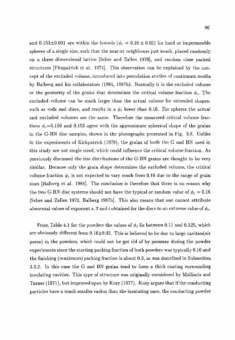
96

and 0.153±0.001 are within the bounds (¢>c = 0.16 ± 0.02) for hard or impermeable

spheres of a single size, such that the near =st neighbours just tOllch, placed randomly

on a three dimensional lattice [Scher and Zallen 1970], and random close packed

structures [Fitzpatrick et al. 1974]. This observation can be explained by the con

cept of the excluded volume, introduced into percolation studies of continuum media

by Balberg and his collaborators (1984, 1987b). Normally it is the excluded volume

or the geometry of the grains that determines the critical volume fraction ¢>c' The

excluded volume can be much larger than the actual volume for extended shapes,

such as rods and discs, and results in a ¢>c lower than 0.16. For spheres the actual

and excluded volumes are the same. Therefore the measured critical volume frac

tions ¢>c=0.150 and 0.153 agree with the approximate spherical shape of the grains

in the G-BN disc samples, shown in the photographs presented in Fig. 3.8. Unlike

in the experiments of Kirkpatrick (1979), the grains of both the G and BN used in

this study are not single sized, which could influence the critical volume fraction. As

previously discussed the size distributions of the G-BN grains are thought to be very

similar. Because only the grain shape determines the excluded volume, the critical

volume fraction ¢>c is not expected to vary much from 0.16 due to the range of grain

sizes [Balberg et al. 1984]. The conclusion is therefore that there is no reason why

the two G-BN disc systems should not have the typical or random value of ¢>c = 0.16

[Scher and Zallen 1970, Balberg 1987b]. This also means that one cannot attribute

abnormal values of exponent s, sand t obtained for the discs to an extreme value of ¢>c'

From Table 4.1 for the powders the values of ¢>c lie between 0.11 and 0.125, which

are obviously different from 0.16±0.02. This is believed to be due to large cavities{ air

pores) in the powders, which could not be got rid of by pressure during the powder

experiments since the starting packing fraction of both powders was typically 0.16 and

the finishing (maximum) packing fraction is about 0.3, as was described in Subsection

3.3.2. In this case the G and BN grains tend to form a thick coating surrounding

insulating cavities. This type of structure was originally considered by Malliaris and

Turner (1971), but improved upon by Kusy (1977). Kusy argues that ifthe conducting

particles have a much smaller radius than the insulating ones, the conducting powder

97

will tend to coat the insulating particles. Then, if the two or three dimensional

two phase powder coating the voids is beyond the pe!"colation limi~, the resulting

composite will be conducting but with a low value of <Pc. The practical minimum <Pc

for this model is about 0.03. For <Pc ~ 0.1, according to Kusy's curve shown in Fig.

2.2, the ratio of the radii is about 7. Therefore, if the average size of cavities is of

about 7 times the typical size of graphite grains, this could leads to a <Pc of about

0.10.

The conductivity exponent t

From the stress-strain experimental results, given in Subection 3.2.3, the structure

of the G-BN disc system belongs to the inverted Swiss-cheese model, which predicted

universal values of 1.7"-'2.0 for the conductivity exponent. The observed conductivity

exponents, t = 2.6 ,,-,2.9 for the disc and parallelepiped systems, are very different

from the universal value. Within the inverted Swiss-cheese model, Balberg (1987a)

suggested that barrier tunnelling of the charge carriers between the conducting grains

in the backbones can give rise to a larger t exponent. As there is no oxide or polymer

coating between the conducting G grains or clusters, tunnelling on the backbones of

the G-BN percolation systems can be ignored. In Fig. 4.4, it is seen that one can

fit the conductivity data in the range of 0.15 < <P <0.82, with a single conductivity

exponent and nearly equally good statistical probability near and far away from <Pc.

Furthermore, Fig. 4.5a shows that the powder conductivity data, in the axial and

transverse directions, can be fitted to the percolation equation on the conducting side

over a range of about seven orders of magnitude in the conductivity, including points

very near the critical volume fraction. This is strong evidence that a single metal

conduction mechanism controls the conduction process on the conducting side.

A further consideration is the influence of the "hollow" cavities. As previously

discussed in this subsection the powders should be visualized as a conductor-insulator

mixture of two components, which coats the air filled cavities. As a powder system

approaches and goes through the percolation threshold, the powder "coating" density

increases and the cavities shrink (some may even vanish). Although the axial and

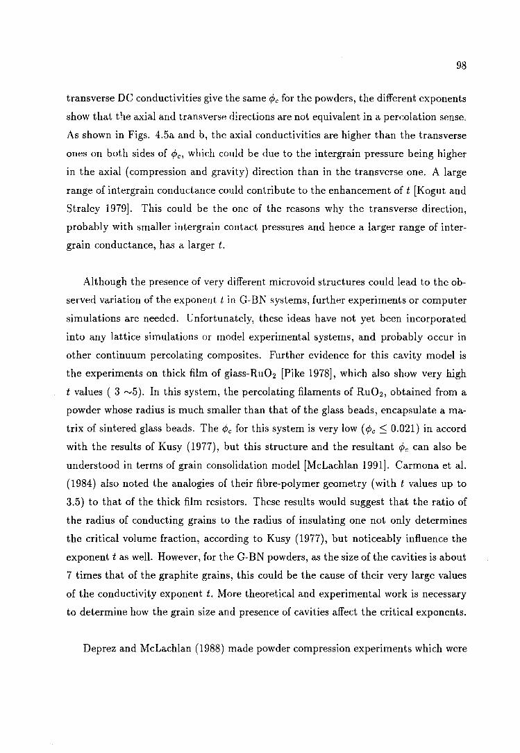
98

transverse DC conductivities give the same cPc for the powders, the different exponents

show that t b.e axial and transversp- directions are not equivalent in a percolation sense,

As shown in Figs. 4.5a and b, the axial conductivities are higher than the transverse

ones on both sides of cPc, which could be due to the intergrain pressure being higher

in the axial (compression and gravity) direction than in the transverse one. A large

range of intergrain conductance could contribute to the enhancement of t [Kogut and

Straley 1979]. This could be the one of the reasons why the transverse direction,

probably with smaller intergrain contact pressures and hence a larger range of inter

grain conductance, has a larger t.

Although the presence of very different microvoid structures could lead to the ob

served variation of the exponent t in G-BN systems, further experiments or computer

simulations are needed. Unfortunately, these ideas have not yet been incorporated

into any lattice simulations or model experimental systems, and probably occur in

other continuum percolating composites. Further evidence for this cavity model is

the experiments on thick film of glass-Ru02 [Pike 1978], which also show very high

t values ( 3 "-'5). In this system, the percolating filaments of RU02, obtained from a

powder whose radius is much smaller than that of the glass beads, encapsulate a ma

trix of sintered glass beads. The cPc for this system is very low (cPc :S 0.021) in accord

with the results of Kusy (1977), but this structure and the resultant cPc can also be

understood in terms of grain consolidation model [McLachlan 1991]. Carmona et al.

(1984) also noted the analogies of their fibre-polymer geometry (with t values up to

3.5) to that of the thick film resistors. These results would suggest that the ratio of

the radius of conducting grains to the radius of insulating one not only determines

the critical volume fraction, according to Kusy (1977), but noticeably influence the

exponent t as well. However, for the G-BN powders, as the size of the cavities is about

7 times that of the graphite grains, this could be the cause of their very large values

of the conductivity exponent t. More theoretical and experimental work is necessary

to determine how the grain size and presence of cavities affect the critical exponents.

Deprez and McLachlan (1988) made powder compression experiments which were

99

analogous to the present ones, except that the measurements were made using four

different pllfe graphite powders and therefore for <Pc < <P < 1. They obtained t( <Pc) val

ues, for the axial and the transverse directions respectively, of 1.94(0.295) & 2.8(0.27),

2.7(0.315) & 2.7(0.33), 1.52(0.27) & 2.1(0.25), and 1.5(0.38) & 2.4(0.37). These re

sults show that both an anisotropic conductivity and different shapes of particles can

give rise to different t and <Pc values, in single powder compression experiments. In

the present case, the abnormally large t value in the powders is attributed to the

number and nature of the cavities and voids as well as a larger range of intergrain

conductances.

Another possible explanation for the large t values that must be considered is the

anisotropy of the conductivity. To date this phenomenon has only been extensively in

vestigated experimentally and numerically in two dimensional systems[Nan 1993 and

references therein]. It has been found that while the t value in one direction increases

with anisotropy, in other direction it decreases. This could be, but is probably not, a

feature of two dimensional systems only. Therefore as t is larger than the universal

value in both systems and approximately equal in both directions for the compressed

discs, this "mechanism" can probably be ruled out.

The differences in the <Pc and t values measured for the "fully" compressed discs

and powders undergoing compression, show that they belong to different classes of

conductivity experiments. The conclusion of the above arguments is that the porosi

ties, including large cavities, in continuum samples give rise to changes in the critical

volume fraction <Pc and possibly in the conductivity exponent t.

The exponents sand s

The expected value for the exponent s from computer simulations is in a range

of 0.87 ",,0.89 [Stauffer and Aharony 1994]. From Table 4.1 it can be seen that a

large range of sand s values have been observed in the present experiments. For the

compressed discs, the s values, obtained from the real part of the dielectric constant,

is clearly smaller than s, obtained from DC conductivity data on the insulating side,

100

while for the poured powders undergoing compression the reverse is usually the case.

U Dfortunately, br powders poured by rotrttion, this is again reversed. An '~xamina

tion of the powder results show that the ¢>c values observed from different pouring

methods are closer to each other than either the s or s values. This shows that the

exponent sand s are probably more sensitive to the microstructures of the discs and

powders than is ¢>c. However, this does not appear to be the case for the exponent

t. As previously argued for the exponent t, the DC axial s value, which is greater

than the universal value of s, cannot be accounted for using the inverted Swiss-cheese

structure of the G-BN discs.

The values of s in this thesis appear to be the first obtained by ultra high resistiv

ity measurements. It should be noted that the s values observed from the resistivity

measurements are generally in disagreement with the s value obtained from dielectric

measurements. In case of the two sets of disc samples, the s values from dielectric

measurements is about half that from resistivity measurements. This would imply

that the exponent s obtained from resistivity measurements could belong to another

class of critical exponents. However, it could be due to the anisotropic conductivity

of the graphite or some other specific feature of the G-BN systems. Further progress

in this direction could not be made in this thesis.

An examination of previous values obtained for s from experimental dielectric

measurements gives s = 0.73 for silver particles embedded in KCI matrix [Grannan

et al. 1981], s = 0.68 for amorphous carbon in teflon [Song et al. 1986], and s = 0.55

and s = 0.62 for filamentary and nodular nickel in polypropylene respectively [Chen

and Johnson 1991]. These values are higher than those obtained from disc dielectric

measurements for both sets of the G-BN disc samples. However, a pattern is emerg

ing that the values of s for comparable three dimensional continuum systems tend

to be lower than the ("theoretical" or "universal") values obtained from computer

simulations.

101

4.3 The Complex AC Conductivity

All the measurements of frequency-dependences of AC conductivity and dielectric

constant were made in axial direction at room temperature in a frequency range from

30H z to 1 OOMH z for the disc samples and from 30H z to lOMH z for the powders un

dergoing compression. The relevant experimental details for these experiments have

been described in Section 3.3.

The experimental results for A C conductivity a-( <p, w) and dielectric constant

c( <p, w), obtained from G-BN disc samples, 50%G-50%BN and 55%G-45%BN pow

ders, will be presented and discussed in terms of the intercluster polarization model,

as discussed in Subsection 2.3.2.

4.3.1 The Exponents x and y

Figs. 4.6a, band c show the AC conductivities versus the applied frequency on a

log-log scale, for the selected samples, with graphite volume fractions near the perco

lation threshold. For <P < <Pc, the AC conductivities increase linearly with the signal

frequency. Above <Pc, the samples show no dispersion in the low frequency range, as

the conductivity is seen to be essentially constant. A DC-AC crossover frequency Wc

exists, beyond which the conductivity starts to increase with frequency, and eventu

ally, in some cases very close to <Pc, shows a linear behavior on a log-log plot, i.e. a

power-law behavior. The crossover frequency Wc increases continuously as (<p - <Pc), or

the DC conductivity, increases. It should be noted that, at high frequencies, there is

no difference in the dispersion of the insulating and conducting samples close to the

critical volume fraction, as the slopes have approximately the same value. In contrast,

the lack of dispersion in the low-frequency range distinguishes the conducting samples

from insulating ones, which allows an estimate of the critical volume fraction <Pc to

be made. For example, it can be seen from Fig. 4.6a that there is a flat response for

.-8 -e---b

102

10-2

a a a a a a a a a a a a a a

• • iI . 10-4 • • I • • • • • • • • • v • ij! ~ • V

8 • 8 + v 10-0 8 + • V 8

8 8 8 8 8 + • 8 V + • v

+ • 10-8 + V • + • v + + • v

• v +

10-10 • V • V V

v

10-12

101 103 105 107

CO(Hz)

Fig. 4.6a The axial AC conductivities against frequency for the disc samples. ¢ =0.168(0), 0.158(.), 0.152(8), 0.150(+), 0.148(_),0.139(\7). The CPc obtained from the DC conductivity data is 0.150±0.001.

.-8

-e---b

103

10-4 " e e e e e e e e e e e e 0

0 0

I 0 <> <> <> <> <> <> <> <>

I )I 8 10-6 )I I

)I )I II i 8 )I )I )I )I )I )I II i II e 8

II II + g

II II II II e i 1 0-8 ~

e + e + A g .

e • e e e A 8 + • + A 8 • + A 8

10-10 • + A 8 • + A 8 • A 8 • l!J 10-12

101

103

105 10

7

m(Hz)

Fig. 4.6b The axial AC conductivities against frequency for the 50%G-50%BN powder. Here cPc= 0.114±0.001. ¢ = 0.130(8), 0.124(0),0.118(*), 0.116(~), 0.115(EB), 0.113(+), 0.111(6), 0.109(_), 0.107(\7), 0.101(0)·

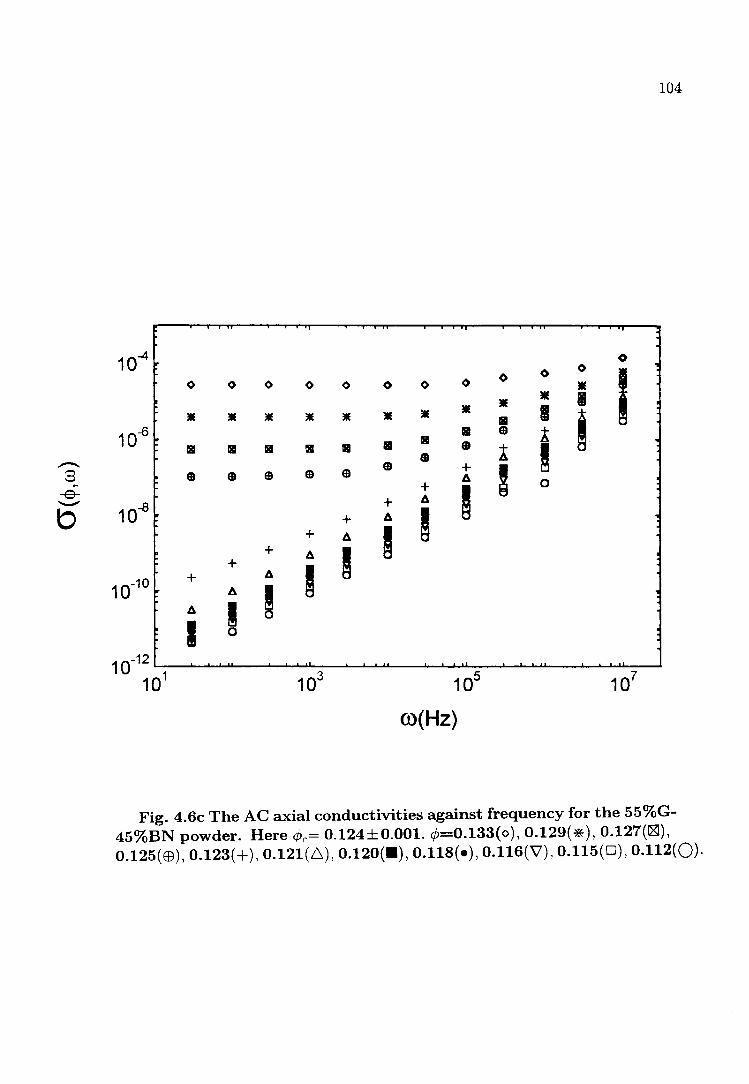
.-S

-e---b

104

10-4 <> , <> <>

I <> <> <> <> <> <> <> <> <> • • • I • • • • • • • • I I III

10-6 III ED i III III III III III III III ED +

~ ED ED A-

ED ED ED ED ED + ! A-+ !

0

10-8 + A-

+ A- I + A- ! + A- ! +

10-10 + A- I A- I A- I 0

I 0

10-12

101 103 105 107

c:o(Hz)

Fig. 4.6c The AC axial conductivities against frequency for the 55%G-45%BN powder. Here cPc= 0.124±0.001. ¢=0.133(o), 0.129(*), 0.127(~), 0.125(63),0.123(+),0.121(6),0.120(_), 0.118(-), 0.116(V'), 0.115(D), 0.112(0)·

105

frequencies lower than 10kHz for cP=0.152 sample, while the frequency response is

linec.rly increasing over the whol~ frequen':y range for the cP=0.150 si\mple. There is

no sample with a volume fraction cP between 0.152 and 0.150. Therefore the value of

the critical volume fraction cPe for the disc system can be estimated to be in the range

of 0.150", 0.152, which is in agreement with cPe=0.150±0.001 obtained by fitting the

two percolation equations simultaneously to the DC conductivity data.

The observed frequency dependence of the conductivity can be explained qualita

tively in terms of the intercluster polarization, as was done by Song et al. (1986), and

Chen and Johnson (1991). For cP > cPe and in the low frequency range, the current

through a sample is almost entirely carried by the backbone, which consists of inter

connected metal (graphite, in this case) clusters, because the capacitive "junctions",

between neighboring finite clusters, form very high-impedance paths at the low fre

quencies. Consequently, the AC conductivity at these low frequencies differs only

slightly from its DC value. As the frequency increases, the impedance of the inter

cluster capacitive junctions decreases and as a result the current can also flow along

these low reactive impedance paths, which do not always incorporate into the back

bone. Therefore the observed AC conductivity near cPe results from two mechanisms:

the capacitive impedance paths shunted by the backbone. At higher frequencies, the

capacitive paths offer lower impedances as they have become more conducting and

can finally short circuit most of the conducting path along the backbone, which results

in the power-law behavior in w for the insulating samples. Near the critical volume

fraction cPe (cP ~ cPe), there exist only a few filamentary percolating paths consisting of

very small clusters and this makes the impedance of the capacitive paths comparable

to that of the resistive ones at low frequencies. Thus We will become lower than that

of samples well above cPe. For cP < cPe, the impedances of the capacitive junctions

will be predominant over whole frequency range, as there is no DC percolating path

through the sample.

According to the scaling law discussed in Subsection 2.3.2, the scaling function

g+ depends only on wjwe • Figs. 4.7a, b, and c show the reduced AC conductivity

--e-'-' b

106

100

1

0.01~7--~~--~-4--~~~~1--~~--~2--~~--~5~

10- 10 10- 10 10

m/roe

Fig. 4.7a The scaled axial AC conductivity cr(¢,w)/cr(¢, 0) against the scaled frequency w jwc for the disc samples. The straight line is a powerlaw fit to the scaled data in the high-frequency regime. The slope is x = 0.82 ± 0.02. cjJ =0.168(0), 0.158(-), 0.152(8).

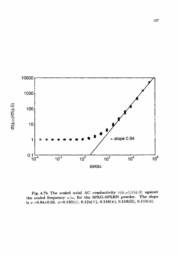
107

10000r-----~----~------------------------

1000

..-o -e- 100 -b -..-8 ~ -b

10

1 9....... (-slope 0.94

OJ/OJc

Fig.4.7h The scaled axial AC conductivity cr(¢,w)/cr(¢,O) against the scaled frequency w/wc for the 50%G-50%BN powder. The slope is x =0.94±0.02. ¢=0.130(e), 0.124(<», 0.118(*), 0.116([81), 0.115(EB).

--a -e-""--' b -....-.. 8

108

1000

100

10

1 ~ slope 0.87

0.1~-4~~~~L2~~~~~O~~~~~2~~--~74~~~~6

10 10- 10 10 10 10

m/mc

Fig. 4.7c The scaled axial AC conductivity CJ(c/J,w)/CJ(c/J,O) against the scaled frequency w/w(, for the 55%G-45%BN powder. The slope is x = 0.87 ± 0.02. c/J=0.133(o), 0.129(*), O.127(rgJ), 0.125(EB).

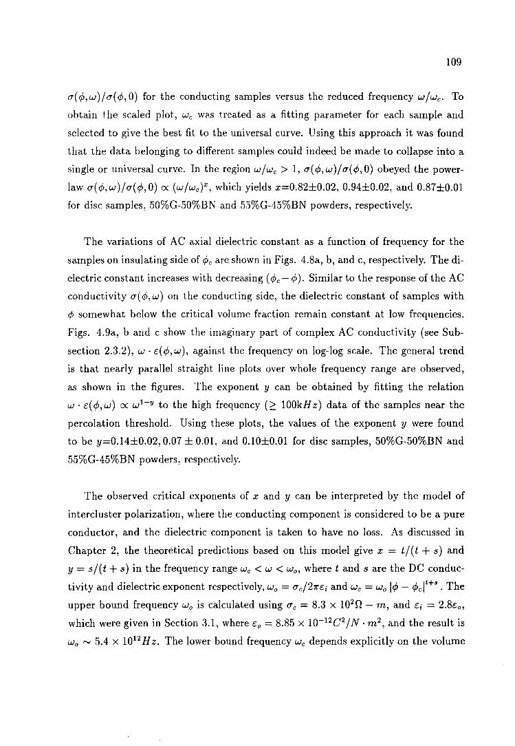
109

(7(e/>,W)/(7(e/>,O) for the conducting samples versus the reduced frequency w/we. To

obtain t he scaled plot., We W?,s treated as a fitting parameter for each sample and

selected to give the best fit to the universal curve. Using this approach it was found

that the data belonging to different samples could indeed be made to collapse into a

single or universal curve. In the region w/we > 1, (7(e/>,w)/(7(e/>,O) obeyed the power

law (7(e/>,w)/(7(e/>,O) ex (w/we)X, which yields x=0.82±0.02, 0.94±0.02, and 0.87±0.01

for disc samples, 50%G-50%BN and 55%G-45%BN powders, respectively.

The variations of AC axial dielectric constant as a function of frequency for the

samples on insulating side of e/>e are shown in Figs. 4.8a, b, and c, respectively. The di

electric constant increases wi th decreasing (e/>e - e/». Similar to the response of the AC

conductivity (7( e/>, w) on the conducting side, the dielectric constant of samples with

e/> somewhat below the critical volume fraction remain constant at low frequencies.

Figs. 4.9a, band c show the imaginary part of complex AC conductivity (see Sub

section 2.3.2), W . c( e/>, w), against the frequency on log-log scale. The general trend

is that nearly parallel straight line plots over whole frequency range are observed,

as shown in the figures. The exponent y can be obtained by fitting the relation

W . c( e/>, w) ex w1- y to the high frequency (~ 100kHz) data of the samples near the

percolation threshold. Using these plots, the values of the exponent y were found

to be y=0.14±0.02, 0.07 ± 0.01, and 0.1O±0.01 for disc samples, 50%G-50%BN and

55%G-45%BN powders, respectively.

The observed critical exponents of x and y can be interpreted by the model of

intercluster polarization, where the conducting component is considered to be a pure

conductor, and the dielectric component is taken to have no loss. As discussed in

Chapter 2, the theoretical predictions based on this model give x = t / (t + s) and

y = s/(t + s) in the frequency range We < W < Wo, where t and s are the DC conduc

tivity and dielectric exponent respectively, Wo = (7e/21rci and We = WO Ie/> - e/>el t+s • The

upper bound frequency Wo is calculated using (7e = 8.3 x 1020 - m, and Ci = 2.8£0'

which were given in Section 3.1, where Co = 8.85 x 1O-12 C2/N· m 2, and the result is

Wo '" 5.4 X 1012 Hz. The lower bound frequency We depends explicitly on the volume

.-8

-e--W

110

100 + + + + + + + + + +

b. b. b. b. b. b. b. b. + b. b. b. + b. A

10 • • • • • • • • • • • • ! • • • • • • • • • • • • • • • • v v v v v v v v v v v v v V 0 0 0 0 0 0 0 0 0 0 0 0 0 0 a a a a a a a a a a a a a a

1 101 103 105 107

CO(Hz)

Fig. 4.8a The axial AC dielectric constant c( ¢, w) (¢ < cPc) against frequency for the disc samples. ¢ = 0.150(+),0.139(6),0.131(_),0.123(-), 0.098(V'), 0.057(D), 0.000(0).

-8 -e--~

111

+ 20

+ + + + A +

A + + A A A + A • • • A A + • • A + • • • • A + • • A 11

10 v • • • • • • • • v • • v v v v v v v • • • 0 8 0 0 0 0 8 8 v B v 0 0 0 0 0 8 8 0 8

5~~~~--~~~~~~--~~~~~~--~~~~

101 103 105 107

co (Hz)

Fig. 4.8b The axial AC dielectric constant E(¢,W) (¢ < ¢c) against frequency for the 50%G-50%BN powder. ¢ =0.113(+), 0.111(6), 0.109(_), 0.107(-), 0.105(V'), 0.103(0), 0.101(0)·

..--.. ':::l '-.J

~ ---W

112

50 + +

+ +

+ +

Ii Ii + + Ii Ii Ii + 20 Ii Ii + • • • • Ii + • • Ii • • • + • • • • Ii • • • • • Ii

V V V • • • v v v v v • • v • v v v 10 0 0 0 0 0 0 0 0 0 0 0 0

a a a a a a a a a a a a

5 10

1 103 105 10

7

ro(Hz)

Fig.4.8c The axial AC dielectric constant c(¢,w) (¢ < ¢c) against frequency for 55%G-45%BN powder. ¢=0.123(+), 0.121(6), 0.120(_), 0.118(.), 0.116(V'), 0.115(D), 0.112(0).

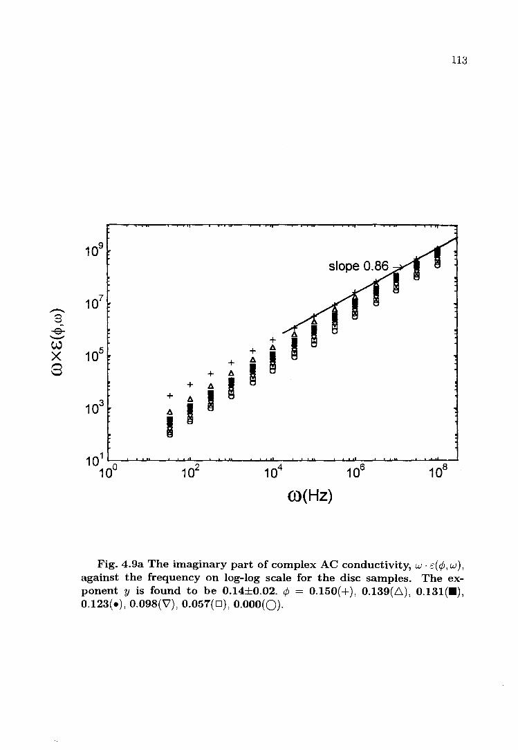
.-8

-e--W X 8

113

107

105 + + ~

+ ~ I + ~ I + ~ I 103 ~ I I

101

10° 102 104 106 108

ro{Hz)

Fig. 4.9a The imaginary part of complex AC conductivity, W· E(¢,W), against the frequency on log-log scale for the disc samples. The exponent y is found to be 0.14±0.02. ¢ = 0.150(+), 0.139(6), 0.131(_), 0.123(-),0.098(\7), 0.057(D), 0.000(0).

114

slope 0.93 ~

Fig. 4.9b The imaginary part of complex AC conductivity, w· E(c/J,w), against the frequency on log-log scale for the 50%G-50%BN powder. The exponent y is found to be 0.07±0.01. c/J =0.113( +),0.111(6),0.109(_), 0.107(-),0.105(\7), 0.103(D), 0.101(0).

115

Fig. 4.9c The imaginary part of complex AC conductivity, w· c(¢,w), against the frequency on log-log scale for the 55%G-45%BN powder. The exponent y is found to be 0.10±0.01. ¢ =0.123(+), 0.121(6), 0.120(.),0.118(-),0.116(\7), 0.115(D), 0.112(0).

116

fraction cPo The calculated and observed values of We (see the next subsection) for

each sample are given in Table 4.2. These results !Show that the frequency ranges

used to derive the exponents x and yare within the estimated frequency bounds of

the scaling law (we < W < wo). Using the values of the critical exponents t=2.63 and

s=0.53, given in Table 4.1 for disc samples measured in the axial direction, one gets

x=0.83 and y = 0.17, which are consistent with the observed values based on the AC

conductivity and dielectric constant data for the disc samples. For the 50%G-50%BN

powder, the values of x and y derived from its DC conductivity exponent t = 4.85

and the low frequency dielectric exponent s = 0.60 are to be 0.89±0.01 and 0.11±0.01

respectively. These values of the exponents x and yare just outside the experimental

error bars of the directly observed values of x = 0.94 ± 0.02 and y = 0.07 ± 0.01.

For the 55%G-45%BN powder, the values of t = 4.80 and s = 0.72 give x = 0.87

and y = 0.13, which are in excellent agreement with the directly observed values

x = 0.87 and y = 0.11. All measured values of two exponents x and y in the three

G-BN systems satisfy the scaling relation x + y = 1 (Equation (2.31)), within the ex

perimental uncertainty. Therefore, the finite cluster polarization can probably model

the AC electric conductivity and dielectric constant near the percolation threshold

for all the three G-BN percolation systems.

In addition to the intercluster polarization effects, the anomalous diffusion of the

charge carriers in the percolation clusters could also make a contribution to the elec

trical conduction of the samples. At higher frequencies, electrons can scan or diffuse

only over a distance Lw '" w-1/(2+ II) < ~ on the conducting clusters, if the clusters are

self-similar fractals. Since the conductivity is predicted to increase with decreasing

Lw [Gefen et al., 1983], the observed conductivity should also increase with increas

ing w. Within the framework of this model, using the Einstein relation between the

diffusion and conduction, and averaging over the contributions of charge carriers sit

uated in different clusters, Gefen et al. (1983) showed that x = t/1/(2 + (}) and

y = (21/ - (3)/1/(2 + ()), where the critical exponents t, 1/, (3 and () have been intro

duced in Section 2.3. Because the exponents 1/, (3 and () cannot be determined for

the samples studied here, one can only use their universal values in three dimensions,

117

Table 4.2 Comparison of the observed cross-over frequencies We (Hz) on the conducting side of the percolation threshold and the theoretical predictions of the R-C model, using the observed exponents t and s.

Discs

<P we(th.) we(exp.) O"de( exp.) 0.152 1.6 x 104 8.3 X 103 2.50 X 10-7

0.158 5.2 x 105 2.0 X 106 4.56 X 10-5

0.168 1.7 x 107 5.7 X 107 1.10 X 10-3

50%G 0.115 2.4 x 10-4 3.0 X 101 2.49 X 10-9

0.116 1.1 x 10-2 3.0 X 102 4.10 X 10-8

0.118 4.6 x 10-1 2.9 X 103 3.43 X 10-7

0.124 6.8 x 101 3.0 X 104 7.37 X 10-6

0.130 8.8 x 102 1.0 X 105 4.69 X 10-5

55%G 0.125 8.9 x 10-3 1.0 X 103 1.02 X 10-7

0.127 3.6 x 10-1 4.0 X 103 5.35 X 10-7

0.129 3.2 x 10° 2.0 X 104 3.82 X 10-6

0.133 5.2 x 101 9.5 X 104 2.71 X 10-5

118

which gives x = 0.58 and y = 0.42. The observed values of the exponents x and

b in all three G-BN semple systems are then clearly in disagreement with the pre

diction of anomalous diffusion model, implying that anomalous electron diffusion in

the backbone does not playa role in the electric conduction mechanism of the G-BN

sample systems in the frequency range observed. It is believed [Gefen et al. 1983]

that anomalous diffusion will only become more important at frequencies higher than

those used in the present work.

The critical exponents x and y have been previously studied experimentally on

various continuum percolation systems. The AC conductivity and dielectric constant

of thin gold films near the percolation threshold were measured by Laibowitz and

Gefen (1984). The thickness of the thin Au films used in their experiments were

in a range 6 "" 10nm and spanned the metal-insulator transition. The frequency

range covered was from 100H z to 10MH z. The power-laws, (2.29) and (2.30), were

observed. These experimental results gave x=0.95±0.05 and y=0.13±0.05. These

values are in agreement with (2.31) within the experimental uncertainty, but are in

dividually different from any of the universal values, which are in two dimensions,

x = y = 0.5, predicted by the intercluster polarization (R-C) model, and x = 0.33

and y = 0.67 from anomalous diffusion model, or in three dimensions, x = 0.72,

y = 0.28 from the R - C model and x = 0.58, y = 0.42 from the anomalous diffusion

model. Nevertheless this experiment was an important step in the characterization

of the full AC response of a percolation system. However, several points remain to

be investigated, such as the influence of the substrate (ShN4 ) at higher frequencies

and the two-dimensional structure of the metallic clusters [Clerc et al. 1990].

Song et al. (1986) studied the AC electrical properties of three-dimensional

amorphous carbon-teflon compacted mixtures, in the frequency range from 10Hz to

13MH z. The experimental values of exponents x and yare 0.86 ±0.06 and 0.12 ±0.04

respectively. These values of the exponent x and yare similar to those obtained for

the G-BN disc samples in the present study, but are also different from the universal

values in three dimensions, predicted by either the R-C model or the anomalous

119

diffusion model. These authors also noted that their exponents were closer to those

found by Laibowitz and Gefen (1984), therefore the thin gold films studied by the

latter might have some three-dimensional properties.

Chakrabarty et al. (1993) measured the complex AC conductance of carbon

paraffin wax mixtures, as a function of frequency from 7Hz to lOOkH z near the per

colation threshold. The exponents were found to be x =0.72±0.01 and y = 0.23±0.05,

which are remarkably close to the three dimensional universal values based on the

R - C model as discussed in Chapter 2. In a recent paper, Lee et al. (1993) in

vestigated the AC conductivity and dielectric constant of carbon black-epoxy bulk

composites over a very wide frequency range from lOOH z to lOGH z. Near the per

colation threshold, the AC conductivity scales as Equation (2.29) with an exponent

x=0.65±0.05 over the full frequency range while the dielectric constant scales as Equa

tion (2.30) with an exponent y=0.26±0.01, in a limited frequency range of 2kHz'"

1.5MH z. In these two carbon-polymer systems, the carbon grains were thought to

be coated with the polymers during the sample preparation. This microstructure is

very different from that of G-BN systems, although the conducting components are

similar in their conductivities. Therefore, as in the G-BN case, there is thought to be

no intergranular tunneling, the difference of the values of critical exponents x and y

between the carbon-polymers and G-BN systems, is not too surprising.

Chen and Johnson (1991) also studied the complex AC impedance of three dif

ferent random metal-insulator composites near their percolation thresholds. Their

three systems include filamentary and nodular shaped nickel particles embedded in

the polypropylene matrix, abbreviated as Ni/F-PP and Ni/N-PP respectively, and

silver particles in the matrix of potassium chloride (Ag-KC1). The AC conductance,

capacitance and dielectric loss tangent of these metal-insulator composites were mea

sured between 5H z and 13MH z. They observed the critical exponents x and y, which

are x = 0.88 ± 0.01, 0.81±0.01 and 0.77±0.01, and y = 0.14 ± 0.01, 0.13±0.04, and

0.22±0.01, for Ni/F-PP, Ni/N-PP and Ag-KCI respectively. Using their DC conduc

tivity and dielectric constant exponents t = 3.1,2.2, and s = 0.55, 0.62 for Ni/F-PP

120

and Ni/N-PP respectively, one can calculate the theoretical values for the exponent

x and y, expected from the R-C model, th!'ough EquatiGns (2.29) and (2.30), whit:h

are x = 0.85, 0.78, and y=0.15, 0.22, respectively. Thus good agreement between

theory and experiment has been obtained for Ni/F-PP and Ni/N-PP, but only if the

experimental (non-universal) sand t values are used.

Hundley and Zettl (1988) investigated the temperature dependence of the expo

nents x and y for a thin-gold-film percolation system, at temperatures between 4.2

and 300K and at frequencies between lOOH z and 1GH z. Their gold films were very

similar to these of Laibowitz and Gefen (1984). Above lOOK, their observed exponents

of x = 0.35 ± 0.05 and y = 0.71 ± 0.05 displayed no apparent temperature effects.

Between 23 and lOOK, both the AC conductivity and the AC dielectric constant still

appeared to scale with frequency but became very temperature dependent. With

decreasing temperatures in this range, the exponent x decreased from 0.35 down to

zero while the y increased from 0.71 up to unity. Below 23K, the AC conductivity

showed no frequency-scaling behaviour, like a homogeneous metal, while the dielectric

measurements became unreliable. Above lOOK, their observed exponent x of 0.35 is

less than the observed exponent y of 0.71, which is contrary to that for the G-BN

systems as well as the other percolation systems discussed above. This difference has

not yet been resolved.

In conclusion, the values of exponents x and y, obtained by Chen and Johson

(1991), and the present work, seem to be fairly similar. These results can all be rea

sonably interpreted by the intercluster polarization model, using the experimentally

measured values of exponents t and s. However, it must also be noted that the values

of the conductivity exponents t for these systems are noticeably different from one

another.

121

4.3.2 The Crossover Frequency We and Exponent q

Figs. 4.10a, b, and c show the experimental crossover frequency We as a function

of sample DC conductivity 0-( <p, 0) on a log-log scale for the samples on the conduct

ing side. The same results are also presented in Table 4.2 (page 117) for comparison

with the theoretical predictions. It is seen from this table that for the G-BN discs

the observed values of the crossover frequency We are in fairly good agreement with

the predictions of the R-C model, using the measured exponents t and s. One salient

feature of this table is that for the powders the calculated We, which explicitly depends

on the t value, is several orders of magnitude smaller than the directly observed one,

partially due to the extraordinarily large values of t. However, the trend of We as

a function of sample DC conductivity agrees with the predictions of scaling theory,

as illustrated in Figs. 4.lOa, band c. Using least-squares fitting to the power-law

We ex o-q(<p, 0), the exponent q is found to be q=1.03±0.01, 0.84±0.01, and 0.82±0.01

for the disc samples, 50%G-50%BN and 55%G-45%BN powders, respectively. These

measured values of q are consistent with the result, q=0.82, obtained from the thin

gold films at temperatures from 100 to 300K by Hundley and Zettl (1988). Benguigui

(1985) obtained q =1.1 from the mixtures of glass and iron balls with a diameter of

1.2 - 1.5mm. More recently, Chakrabarty et al. (1993) measured q=1.1 in carbon

wax mixtures at room temperature.

Scaling theory, based on the intercluster polarization effects, which was discussed

in Section 2.3, gives an expression for the exponent q in terms of the conductivity

exponent t and dielectric exponent s, which is q=(t + s )/t on the conducting side.

This implies that the values of exponent q can never be less than unity. The directly

observed exponents q = 1.03, 0.84 and 0.82 in this study are in disagreement with the

predicted values of 1.20,1.15 and 1.06, using the measured values of the DC conduc

tivity exponent t and dielectric constant exponent s. A large discrepancy between

the observed exponent ( 0.82 ) and the theoretical value (1.66 in that case) was also

noted in Hundley and Zettl's paper (1988). Although the value of exponent q=1.1,

reported by Benguigui (1985) and Chakrabarty et al. (1993) respectively, are larger

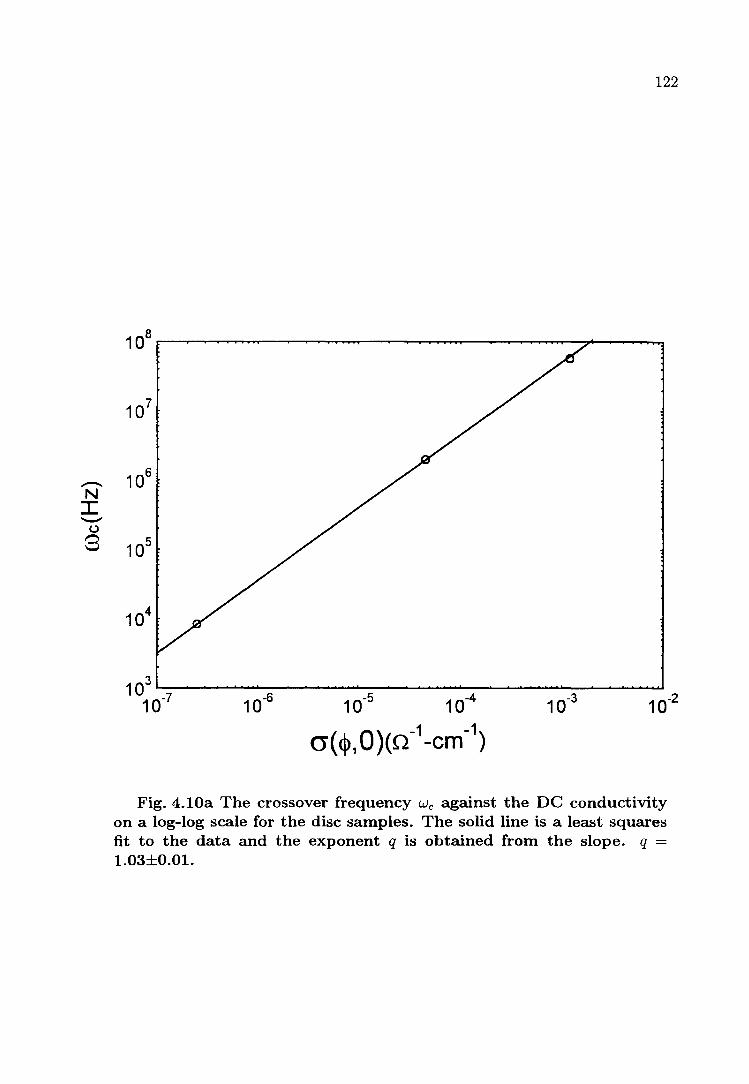
.-. N I -u 8

122

103~--~--~--~~~~--~~~--~~~~--~~~ 1 0-7 1 0-6 1 0-5 1 0-4 1 0-3 1 0-2

cr( <\>,0 )(Q-1_Cm -1)

Fig. 4.10a The crossover frequency We against the DC conductivity on a log-log scale for the disc samples. The solid line is a least squares fit to the data and the exponent q is obtained from the slope. q =

l.03±O.Ol.

123

-N I -(,) 8 103

101~~~~~~~~~--~~~~~~~~~~~~ 10-9 10-8 10-7 10-6 10-5 10-4

(j(~,O)(n-1_cm-1)

Fig. 4.10b The crossover frequency We against the DC conductivity on a log-log scale for the 50%G-50%BN powder. q =O.84±O.Ol.

.-N I -(,J

124

8 104

10~ 10~

(j(~,O)(n-1-cm -1)

Fig. 4.10c The crossover frequency We against the DC conductivity on a log-log scale for the 55%G-45%BN powder. q =O.82±O.Ol.

125

than unity, these values are still about 30% smaller than the predicted exponents of

1.4 in both cases. Chakrabarty et al. daimed that (;l,n insufficient range of data, which

only span just over one decade in frequency and in the DC conductivity, was responsi

ble for the discrepancy between the observed value and the theoretical prediction for

q. This limitation does not apply to the present study, or that of Hundley and Zettl,

which spans 7 decades and gives still lower values of q. It is clearly observed in Figs.

4.10a, band c that both the crossover frequency data and the DC conductivity data

cover four or more decades, and obey a power-law with a very small scatter in the data.

From Figs. 4.9a, band c, when W • c( <p, w) is scaled (normalized) by the DC con

ductivity 0"( <p, 0) for each value of <p, one gets the scaled plots shown in Figs. 4.lla,

band c, which correspond to Figs. 4.9a, band c respectively. Except the data for

the <p = 0.150 sample shown in FigA.lla, all the curves in each figures almost col

lapse into a single straight line. Since the disc sample with <p=0.150 is just on the

percolation threshold, its different behaviour could probably be ignored. Because no

frequency scaling is necessary to scale the plots of W· c(<p,w), Figs. 4.11a, band c

show that the crossover frequency is We '" 1 for nearly all the G-BN samples on the

insulating side. These results also lead to the conclusion that, using the theoretical

relation We ex:: O"q( <p, 0) and taking into account the different values of the DC con

ductivities of the insulating samples, the exponent q is zero below the percolation

threshold for the three G-BN systems. This value of q=O is in disagreement with the

predictions made by the R-C model, which gives q = - (t + s) /s on the insulating

side. Using the observed values of the exponents t, sand s, the exponents q are found

to be -3, -13 and -12 for the G-BN discs, 50%G-50BN and 55%G-45%BN powder

systems, respectively. Therefore on the insulating side of percolation, the intercluster

polarization model seems not apply to the G-BN systems. No previous experimental

result for We on the insulating side of the percolation threshold is, to the author's best

knowledge, available for comparison.

It has been shown in Section 3.3 that the porosity of the disc samples is about 0.18

while the 50%G-50%BN and 55%G-45%BN powders undergoing compression are even

-0 -v --b -.. ~ -8 V --w x 8 ~

126

25 10

i i 23 i 10 i

i i 21 i + 10 l-

i + + i + I!

i + 19 i + 10 l!- i + i + ,

i + 17 +

10 + . +

+ +

15 10 0 2 4 6

108

10 10 10 10

ro(Hz)

Fig. 4.11a The normalized imaginary part of complex AC conductivity, W· c( 1;, w) / rJ( 1;,0), against the frequency on a log-log scale for the disc samples. q; = 0.150(+), 0.139(6), 0.131(_), 0.123(.), 0.098(\7), 0.057(D), 0.000(0)·

-a --e--b ......... r-'O -8 -e--W x 8 ---..

127

, • • • • • • • • • •

1015~~~~--~~~--~~~~~~--~~~--~~--~

101 103 105 107

CO(Hz)

Fig. 4.11h The normalized imaginary part of complex AC conductivity, W . E(¢,W)/(J'(¢, 0), against the frequency on a log-log scale for the 50%G-50%BN powder (¢ < ¢c). ¢=0.113(+), 0.111(6), 0.109(_), 0.107(.), 0.105(V'), 0.103(0), 0.101 (0).

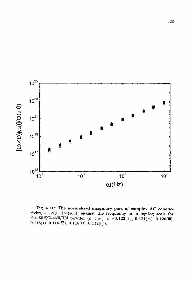
...-a --e---b ........ .....-...-8

-e---W X 8 .......

128

1023

III III ,

1021 l- I • •

1019 I- ~

@I

~ ~

~ • 1017 Ir

1015L-~~~--~~~~~~--~~~--~~~~--~~ 10

1 10

3 10

5 10

7

CO{Hz}

Fig. 4.11c The normalized imaginary part of complex AC conductivity, W . E( ¢, w) / CJ( ¢, 0), against the frequency on a log-log scale for the 55%G-45%BN powder (¢ < ¢c). ¢ =0.123(+), 0.121(6), 0.120(.), 0.118(-),0.116(\7),0.115(0),0.112(0).

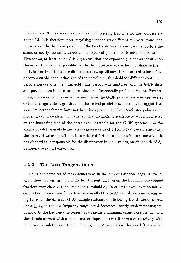
129

more porous, 0.70 or more, as the maximum packing fractions for the powders are

about 0.3. It is therefore most surprising that the very different microstructures and

porosities of the discs and powders of the two G-BN percolation systems produce the

same, or nearly the same, values of the exponent q on the both sides of percolation.

This shows, at least in the G-BN systems, that the exponent q is not as sensitive to

the microstructure and possibly also to the anisotropy of conducting phase as is t.

It is seen from the above discussions that, up till now, the measured values of ex

ponent q on the conducting side of the percolation threshold for different continuum

percolation systems, viz. thin gold films, carbon-wax mixtures, and the G-BN discs

and powders, are in all cases lower than the theoretically predicted values. Further

more, the measured cross-over frequencies in the G-BN powder systems are several

orders of magnitude larger than the theoretical predictions. These facts suggest that

some important factors have not been incorporated in the intercluster polarization

model. Even more alarming is the fact that no model is available to account for q ~O

on the insulating side of the percolation threshold for the G-BN systems. As the

anomalous diffusion of charge carriers gives q value of 1.4 for ¢Y > ¢Yc, even larger than

the observed values, it will not be considered further in this thesis. In summary, it is

not clear what is responsible for the discrepancy in the q values, on either side of ¢Yc,

between theory and experiment.

4.3.3 The Loss Tangent tan [)

Using the same set of measurements as in the previous section, Figs. 4.12a, b,

and c show the log-log plots of the loss tangent tan 8 versus the frequency for volume

fractions very close to the percolation threshold ¢Yc. In order to avoid overlap not all

curves have been shown for each ¢Y value in all of the G-BN sample systems. Compar

ing tan 8 for the different G-BN sample systems, the following trends are observed.

For ¢Y ~ ¢Yc, in the low frequency range, tan 8 decreases linearly with increasing fre

quency. As the frequency increases, tan 8 reaches a minimum value, tan 8m at W m , and

then bends upward with a much smaller slope. This result agrees qualitatively with

numerical simulations on the conducting side of percolation threshold [Clerc et al.

r~

C ro +-'

10

1

0.1

0.01 1 10

~ 6 <> 8 ~ • •

~ slope -0.80

a a

<> <> <> <> ~

~ ~ ~ • • • •

a a <> & ~

• •

105

ro(Hz}

a & •

130

a a i i A A • • •

Fig. 4.12a The loss tangent tanb for the samples very close to the percolation threshold against the frequency on a log-log scale for the disc samples. ¢ =0.152(0),0.150(0),0.139(6),0.131(.).

'.0 C ro .....

131

+-- slope -0.84 10

1 • • • + • • • • + + + i + + + + + + + l.

0.1 l. l. • l. l. l. • l. l. l. l. l. • • • • • • • • • 0.01 1

10 103 105 107

CO{Hz)

Fig. 4.12h The loss tangent tanb for the samples very close to the percolation threshold against the frequency on a log-log scale for the 50%G-50%BN powder. ¢; =0.115(ffi), 0.113(+),0.111(6),0.109(_).

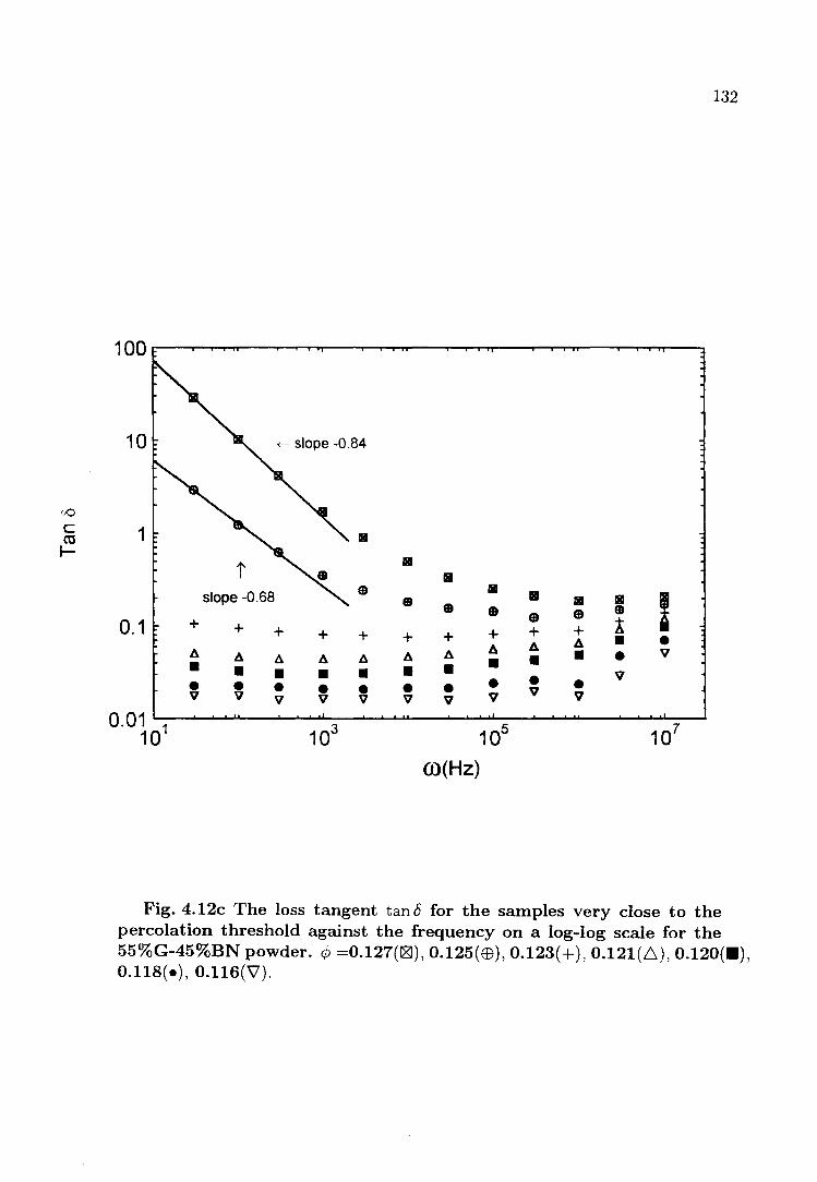
'A)

c CO ~

132

10 ~ slope -0.84

1 III

III t III

slope -0.68 ED II III

! ED II III ED ED ED ED ED

0.1 + + + + + X + + + + + 11 • • 11 11 11 • V 11 11 11 11 A 11 • • • • • • • • • • v • • • • • • • • • • v v v v v v v v v v

0.01 1 10 103 105 107

m(Hz)

Fig. 4.12c The loss tangent tan 8 for the samples very close to the percolation threshold against the frequency on a log-log scale for the 55%G-45%BN powder. ¢ =0.127(1ZI), 0.125(EB), 0.123(+), 0.121(6), 0.120(.), 0.118(.),0.116(\7).

133

1990]. As Chen and Johnson (1991) argued in their paper, for a sample above <Pc, a

l/w dependence of the loss tangent, tan D =l/wRC = r.Tc-/wci ex: l/w, is expected in the

low frequency regime w < W c , where the energy loss in the dielectric is due to the DC

conductance along the backbone. The slopes for the samples just above <Pc are found

to be -0.80 (<p = 0.152), -0.84 (<p = 0.115), and -0.68(<p=0.125) for the discs, 50%G-

50%BN and 55%G-45%BN powders respectively. These values, somewhat different

from -1, may show that the metal-insulator transition of these samples has not yet

been completed. For <P < <Pc, a flat minimum, with a slight dip, in tan D is observed.

As <P approaches <Pc from below, tan D tends to become a constant, or less frequency

dependent, in agreement with the prediction based on the intercluster polarization

model. This phenomenon is attributed mostly to the fact that, below <Pc, there is no

continuous percolating cluster in the samples and the insulating barrier between the

larger conducting clusters dominates the electric (now mainly dielectric) behaviour,

resulting in a smaller, less frequency-dependent, loss tangent [Chen and Johson 1991].

The observed minimum in the loss tangent tan D, as a function of frequency, for

G-BN samples below <PC) is qualitatively inconsistent with the results of computer

simulations in three dimensions reported by the French group [Clerc et al. 1990, and

references therein]. They showed, using the effective-medium approximation (EM A)

and the transfer-matrix algorithm of the R-C model, that there is a global maximum

of loss tangent at the crossover frequency Wc (see Subsection 4.3.2) below the percola

tion threshold. Since the very similar trends in tan D against frequency are observed

in both disc and powder G-BN systems, the difference in the porosities and the bad

electrical contacts between graphite grains in the powder samples are probably not

the cause of the discrepancy between the present experiment and the numerical calcu

lations. Further theoretical and experimental work is required to clarify this "puzzle".

From the minimum of tan D against the frequency just below <Pc, the values of tan Dc

are estimated from Figs. 4.12a, band c, and found to be 0.22±0.02, 0.13 ± 0.02,and

0.09±0.01 for the discs, 50%G-50%BN and 55%G-45%BN powders respectively. Us

ing Dc = Y * (1r /2) (see Section 2.3), the critical exponent y can be calculated from

134

the minima, tan 8e , which gives y=0.14±0.01, 0.08±0.02, and 0.06±0.01 respectively,

These results are reasonably dose to those obtained from the plots of imagina~y part

of the complex AC conductivity versus the frequency, as shown in Figs. 4.9a, b, and Co

Therefore, these two reasonably consistent values of y obtained by different methods

of analysis show that there are some consistencies in the R-C model when applied

to the G-BN continuum systems.

The loss tangent as a function of frequency for percolation systems has been ex

perimentally studied by many authors. Laugier et al. (1986) performed AC electrical

measurements on random mixtures of plain and silver-coated glass microbeads, for

<P < <Pc, in the frequency range from DC to 50MHz. The mean diameter of the beads

was roughly 30jlm, with a dispersion in size of around 50%. They found the min

imum of tan 8 (w) to be 0.55±0.05, in good agreement with the value of 0.47±0.04

expected from the R - C model. They also noted an unexpected increase in the loss

tangent on the low-frequency side of the minimum. This was attributed to the non

vanishing DC conductivity of the glass beads, and was confirmed by the computer

simulation, using a non-zero DC conductivity for the insulating component [Laugier

1987]. This explanation, however, does not apply to the present case of study as the

DC resistivity of BN powder is about 1 x 10160hm-cm and the "dry" air pores in the

powders are even more resistive, because the relative humidity in the air pores is less

than 12% at room temperature when the measurements were made. Therefore it is

not clear what physical information is contained in the slight increase of tan 8 with

decreasing frequency at lower frequencies for <p ::; <Pc in the G-BN percolation systems.

The frequency dependence of AC conductivity and dielectric constant of water / AOT / oil

microemulsions (AOT being the surface-active agent, or surfactant) has been stud-

ied by Van Dijk (1985) and Van Dijk et al. (1986). In this system the water forms

droplets, 5 f'V lOnm in diameter, coated by the AOT, which are far more conductive

than the continuous oil phase because of the ions dissolved in the water. The AC

conductivity was measured in the frequency range from 10kHz to 13MH z. A plot

of tan 8 shows a plateau over nearly two decades of frequency for two or more sam-

135

pIes near </>c, with a value of tan bc=0.67±0.04, which gives y=0.35 from bc=y*( 7r /2).

This is consistent with their value of x=0.62±0.02 and hence y=0.38, obtained us·

ing the method described in Subsection 3.3.1. Chen and Johnson (1991) observed a

frequency-independent loss tangent for Ni/F-PP samples (</>=0.06 and 0.05) close to

the percolation threshold with </> :::; </>c, similar to the G-BN sample systems. They

showed that the measured loss tangent, tan 15, at a given frequency diverges as the

metal volume fraction approaches the percolation threshold from below. This diver

gence obeyed an empirical percolation equation tan 15 ex (</>c - </> )-(t-2s), proposed by

the same authors. However, the power law for the loss tangent that they reported

may be due to an incorrect critical volume fraction </>c=0.08±0.01, which was obtained

by fitting the DC conductivity data on the conducting side only. This value of </>c

is also inconsistent with the AC conductivity data shown in their Fig. 6, where the

samples with </>=0.070 and 0.081 show a plateau as a function of frequency at low

frequencies, indicating that they are on conducting side of the percolation threshold.

Furthermore, as these are the only authors to observe a tan 15 ex (</>c - </> )-(t-2s) re

lationship, one must conclude that this power law may only apply to their (or very

similar) system.

4.4 The Magnetoresistance

Measurements of the Hall coefficient were attempted at room temperature and at

liquid-nitrogen temperature using the previously described G-BN parallelepiped sam

ples, with a length-to-width ratio of 3 [Putley 1960j. A lock-in amplifier, operating

at low frequencies (5,,", 33Hz), and Prema 5000 digital voltmeter with a resolution

of O.1j.lm were both used to try to detect the Hall voltage. Unfortunately, no Hall

signal could be detected by the instruments used, using maximum available magnetic

field of 1.5Tesla and the largest current, typically about 2mA, which can be safely

used without heating the samples. Due to the time limitation of this thesis, further

attempts to improve the Hall instrumentation had to be given up.

The transverse magnetoresistance was measured on the samples (</> > </>c) with the

136

length-to-width ratio of 1/6 at room temperature. The data acquisition was comput

erized so that the measure .nent could be repeated "J 1 0 times at each field to improve

the signal to noise ratio. For the experimental details, see Section 3.4.

The magnetic field induced a change of conductivity, i.e. magneto conductivity.

It is observed that -60-(H= loST) tends to vanish as the percolation threshold <Pc = 0.150 is approached from above, as shown on a log-log scale in Fig. 4.13. The solid line

is the result of a least squares fit of the equation -60- ex (<p - <pc)tm to the data, which

yields the critical exponent tm = 3.07 ± 0.06, using the <Pc of 0.150 found from the

DC conductivity measurements. Fig. 4.14 shows that the relative magnetoresistance

6R(lo5T)/ R also decreases with decreasing graphite volume fraction <p, and varies

as (<p - <Pc)gc, with the critical exponent gc=0.28±0.Olo The difference between the

exponent tm (=3.07±0.06) and t (=2.68±0.13) is 0.39±0.19, which is consistent with

the observed value of the exponent gc, within the quoted experimental errors.

As discussed in Subsection 2.3.4, the magnetoconductivity or relative magnetore

sistance of random metal-insulator percolation composites has been investigated the

oretically by Bergman (1987). In this pioneering work, he used scaling arguments

to predict the behavior of 60- and 6R/ R near a percolation threshold. As Rohde

and Micklitz (1989) pointed out, this calculation gives a critical exponent tm for

the magneto conductivity which is same as the t for the conductivity. Consequently

gc = tm - t = 0, implying that 6R/ R does not vary near the percolation threshold.

These theoretical predictions are in disagreement with the measurements made on

the G-BN samples, shown in Fig. 4.14, where the relative magnetoresistivity exhibits

a dependence upon (<p - <Pc).

The only other experimental study of magneto conductivity and relative magne

toresistivity was made in situ on granular Sn-Ar films with a thickness of 800 -

1000A at a temperature of 4.2K, by Rohde and Micklitz (1989). The films were fab

ricated by coevaporating the metal and the rare gas on a sapphire substrate. They

found the critical volume fraction <Pc to be 0.26 and the critical exponents t, tm and

gc to be 1.6±0.1, lo90±0.15 and 0.30 respectively. This value of gc is consistent with

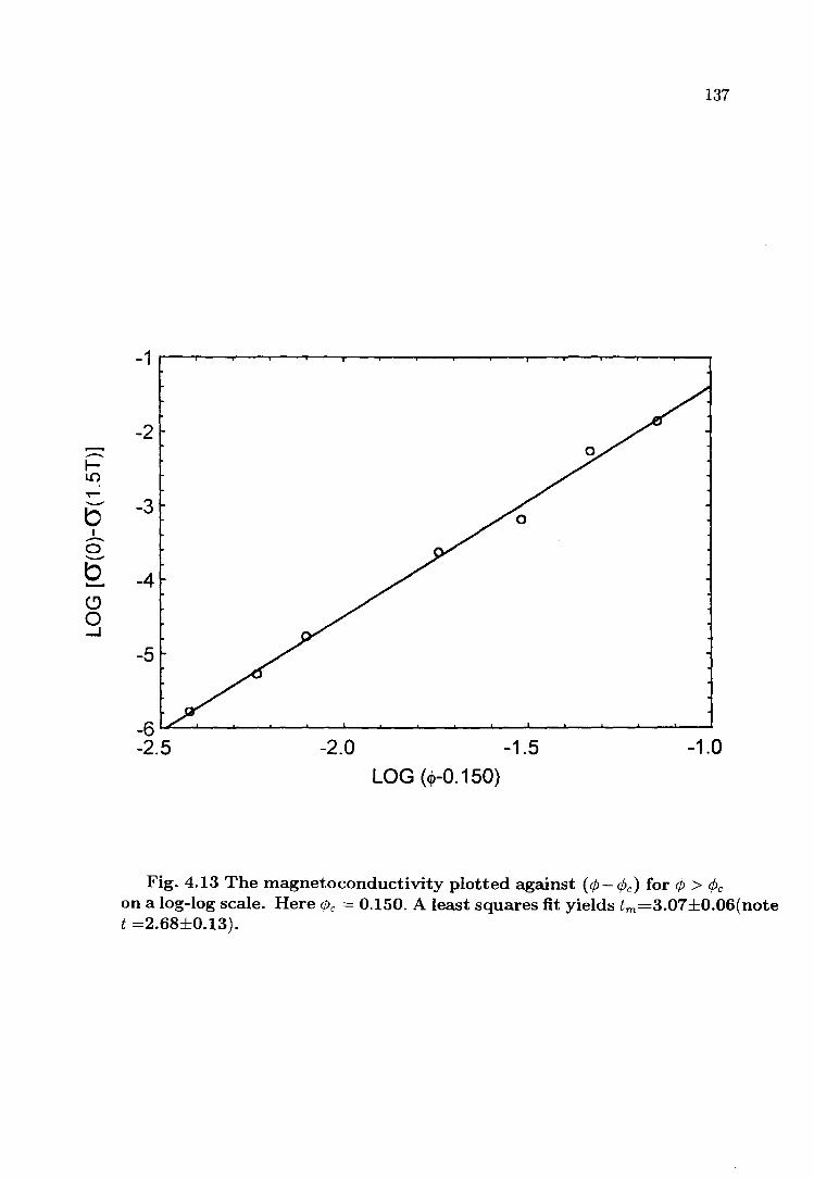
..--. .-I-LO T"" -b

I .-a -b ........ (9 0 ...J

137

-2

-3

-4

-5

-6~~~~~~--~~--~~--~~--~~--~~~

-2.5 -2.0 -1.5 -1.0

LOG (<j)-0.150)

Fig. 4.13 The magneto conductivity plotted against (¢ - ¢c) for q; > ¢c on a log-log scale. Here ¢c = 0.150. A least squares fit yields tm=3.07±0.06(note t =2.68±0.13).

,........, -. o -- -1.7 a::: ----. -. o --a::: -1.8

I -. ~ LO

~ -1.9 --a::: -~ <.!) o -2.0 ....J

138

-2.1~~~~~~--~~----~~----~~----~~--~~~

-2.5 -2.0 -1.5 -1.0

LOG{q,-0.150)

Fig. 4.14 The relative magnetoresistance 6R/R plotted against (1;<P,:) for 1; > 1;c on a log-log scale. Here 1;c =0.150. A least squares fit to the data yields the exponent gc of 0.28±0.01.

139

the one obtained from the G- BN system. Comparing the experimental observations

from the percolation systems G-BN and Sn-Ar, the values of gc are very similar, but

the values of the exponent tm are very different for the two systems and disagree with

the theoretical prediction that tm = t. The G-BN composites and Sn-Ar mixture are

physically very different percolation systems, as indicated by the different conductiv

ity exponents and the different percolation thresholds. The Sn-Ar mixtures gave the

critical exponent t = 1.6 ± 0.1, slightly lower than the generally accepted range of

1.7 - 2.0, while the observed conductivity exponent t = 2.68 ± 0.13 for the G-BN

parallelepiped samples is much larger and definitely nonuniversal. Because they have

the same crystal structures and densities, the graphite and hexagonal boron-nitride

phases in the composites are indistinguishable by topological methods, in contrast to

that of the Sn-Ar mixtures [Rohde and Micklitz 1989J. The agreement in the critical

behavior of the magnetoresistivity in such very different systems indicates that the

observed discrepancy between theory and experiments could be fundamental. Further

measurements of the magnetoresistivity are necessary to check if a gc of 0.28 - 0.30

is "universal" for all disordered systems.

4.5 Summary

Critical volume fractions <Pc=0.150 and 0.153 were observed for two sets of G-BN

disc samples, which are close to the "random" value of 0.16±0.02. For the powders,

the measured values of <Pc are from 0.11 to 0.12, smaller than the random value in

three dimensions. This difference is attributed to the presence of a large number of

cavities, as the packing fraction is about 0.25 at <Pc in the G-BN powders undergoing

compression. Nonuniversal t values were obtained in all three G-BN percolation sys

tems. For the disc samples, the observed t values are about 2.6 and 2.7 in the axial

and transverse directions respectively. For the powders, the values of exponent tare

found to be 4.8 and 6.1 in the axial and transverse direction respectively, which are

approximately three times the universal value in three dimensions. The observed s and s values distributed in a rather broad range 0.4 - 1.1. The observed nonuniver-

140

sal exponent t, sand s cannot be explained by the existing models for non universal

exponents, e.g. the Swiss-cheese model and the inverted Swiss-cheese moriel with

tunnelling.

For the AC conductivity, all the measured exponents x and y for the G-BN discs

and powders have been interpreted in a satisfactory way, using the intercluster polar

ization model and the measured values of t and s. Above the percolation threshold,

the scaling law We ex: a q( </>,0) is observed. Although the measured values of the expo

nent q are smaller than their theoretical predictions using the observed exponents t

and s for the G-BN systems, these somewhat lower than expected values are consistent

with other experimental observations. Below the percolation threshold, the crossover

frequency We is found to be unity and consequently q "" 0, which cannot be explained

using existing percolation theories. A nearly constant or frequency-independent loss

tangent tan be near the critical volume fraction on the insulating side is observed, and

the exponents y derived from the plots of loss tangent versus frequency agrees with

those obtained from W • c( </>, w) versus frequency plots on a log-log scale. The global

minimum in tan b as a function of frequency below </>e cannot be accounted for by the

intercluster polarization model.

The magnetoresistivity exponent (0.28) obtained from the G-BN system at room

temperature and in a magnetic field of 1.5T agrees with the value (0.30) obtained

at 4.2I< in a field of 2T for the three-dimensional granular films of Sn-Ar mixtures

[Rohde and Micklitz 1989]. Both these experimental results are in disagreement

with the theoretical prediction made by Bergman (1987). This discrepancy between

experiment and theory shows the necessity of further experimental and theoretical

magnetoconductivity studies.

141

Chapter 5

THE 1/ f NOISE

5 .1 Introduction

The purpose of the study of 1/ f noise in the G-BN compressed conducting sam

ples (discs and parallelepipeds) close to the percolation threshold is twofold. First,

to verify the power-laws Sv /V2 ex: RW and (<p - <Pc)k in the critical region, which may

assist in the identification of the conduction mechanism on the conducting side of the

percolation threshold. Secondly, to investigate the inhomogeneous structure of the

samples near <Pc, since the voltage fluctuations are more sensitive than the resistance

because the voltage fluctuation is a fourth order moment of the local current whereas

the resistance is of second order [Ram mal et al. 1985b].

There are several theoretical models dealing with the 1/ f noise in percolation

systems. These models include lattice resistor networks, Swiss-cheese and inverted

Swiss-cheese models, and two component effective-medium theories. However, it must

be noted that there is no single 1/ f noise model, which can explain all the experimen

tal results obtained from all measurements to date of continuum percolation systems.

Also many models are designed to explain the results for a single experimental system.

As previously stated in Section 3.5, the 1/ f noise in the conducting G-BN disc

samples near the percolation threshold was measured in both the axial and transverse

142

directions in the frequency range 1Hz", 1000Hz at room temperature. Six or seven

different DC currents were used to check th~ F-dependence. The noise power spectra

measured as a function of the frequency are found to be close to 1/ f in all the G-BN

conducting samples measured and at all current levels used. The measured noise

spectrum can be characterized by the Hooge's empirical formula (2.48), which is

rewritten here for convenience as

a V'I? Sv---- NT/ f'Y' (5.1 )

where the symbols are already defined in Section 2.3.3.

Using the fractal structure of infinite percolation cluster near <Pc, Rammal and

his co-workers (1985b) predicted that near the percolation threshold the normalized

1/ f noise power scales as Sv /V 2 ex L -b, where L (>0 is the linear dimension of

the sample and b=1.18",1.26 in a three dimensional resistor network lattice. Unfor

tunately, this theoretical prediction still lacks experimental support. This chapter

will give the experimental results of the sample size dependence of the 1/ f noise in

the compressed G-BN samples. The measurements of size dependence of normalized

1/ f noise power were, to a certain extent, to try to reveal the fractal structure of

the percolation cluster in the G-BN disc samples. The 1/ f noise was measured on

several conducting samples near the percolation threshold, where the sample volume

was decreased in such a way that the thickness of sample was kept constant, while the

length and width were decreased with the same length-to-width ratio for each sample.

The rest of this chapter is organized as follows. The experimental results, with

constant sample volume, are presented and discussed in Section 5.2. The sample

size dependence of the normalized 1/ f noise is given in Section 5.3. The chapter is

concluded in Section 5.4.

143

5.2 Sv/V2 as a Function of Sample Resistance

Figs. 5.la and b show the normalized noise power spectra Sv(J)/V2 (with the

background noise subtracted off) against the frequency for seven samples both in the

axial direction (disc-shaped ) and in the transverse direction ( parallelepipeds of the

same dimensional size) respectively. These figures show that the noise spectrum can

be fitted to the relation Sv(J)/V2 ex f-'Y. The values of the exponents, are obtained

by using least squares fits, and the values are summarized in the columns 2 and 3

of Table 5.1. The exponent, varied in the range 0.95-1.08 with a weighted mean

(see Section 3.7) of 1.0l±0.01 in the axial and 1.06±0.01 in the transverse direction

respectively. It is seen from these plots that, within the experimental error, there is

no significant difference in the values of the exponent, in the transverse and axial

directions.

The current dependences of noise power magnitude at 10Hz for each sample are

illustrated on a log-log scale in Figs. 5.2a and b. The lines drawn through each

sample data points are the results of least squares fits to the data. The columns 4

and 5 of Table 5.1 list all the values of exponent {) determined by the slopes of lines

through the data points. Similar results are obtained at other fixed frequencies in

the range 1Hz", 1000Hz. In general the noise varies with I, for small currents and

independent of frequency, with a power just less than 2. The averaged values of the

exponents {) are found to be 1.96±0.01 and 1.93±0.02 in the axial and transverse

directions respectively. From Equation (5.1) an I2-dependence is expected for noise

generated by resistance fluctuations in the composites probed by DC current, and is

usually found for "1/ f " noise systems

Fig. 5.3 shows the normalized noise power at 10Hz, as a function of the sam

ple resistance, near the percolation threshold, in the axial and transverse directions.

The least squares fits of a straight line to the relevant data yield two exponents

N

< > en

144

10-8 • 9 9 0 999 0 0

0 o c Cc 000

10-10 • • • ••• • •

10-12 A • •• A A AAA

10-14

slope -1.0

10-16 a 1 10 100 1000

f (Hz)

Fig. 5.1a The normalized noise power against the frequency in the axial direction. The volume fractions from top to bottom are ¢ =0.152("9), 0.158(0), 0.156(0), 0.168(.), 0.180(_), 0.197(6), 0.221(+). The values of the exponents I are given in Table 5.1.

N

< > en

145

10-6 0 v 0

0 v '11 000 v V'll

10-8 0 0

DOD

• ... 0:---10-10 • • ... • • ••• a

0. 0.*:", , 10-:2

* III :* L 10-14

slope -1.0

• 10-16

1 10 100 1000

f (Hz)

Fig. 5.1b The normalized noise power against the frequency in the transverse direction. The volume fractions from top to bottom are ¢ =0.152(0), 0.156(V'), 0.158(0), 0.168(-), 0.180(_), 0.221(+), 0.197(6). The values of the exponents, are given in Table 5.1.

146

Table 5.1 The observed values of the exponents, and {) in the axial and transverse directions respectively.

Axial ¢ , uncertainty {) uncertainty Ill, in {)

0.152 1.024 0.002 1.977 0.045 0.156 0.976 0.002 1.868 0.035 0.158 1.019 0.002 1.940 0.038 0.168 1.018 0.002 1.990 0.020 0.180 1.027 0.003 2.020 0.031 0.197 1.015 0.002 1.952 0.032 0.221 1.039 0.005 1.980 0.035

Transverse 0.152 1.134 0.004 1.817 0.055 0.156 1.047 0.003 1.826 0.044 0.158 1.045 0.003 1.804 0.082 0.168 1.045 0.002 2.068 0.056 0.180 1.029 0.003 2.093 0.053 0.197 1.065 0.002 1.980 0.037 0.221 1.095 0.004 1.810 0.066

...-N I 0 ~ ---> U)

<.9 0 --l

147

-9.0

-10.5

-12.0

-13.5

-1 5. 0 1L....&.--£.......i.-...L--1.......J,.---'----"--'--.J..........I____'_--'--~...L.......I:'___'____'_'II~__'__..&...._..I____'_~ -6 -5 -4 -3

LOG I(amp)

-2 -1

Fig. 5.2a The noise power in the axial direction against the DC current on a log-log scale. The solid lines are least squares fits to the data. From right to left ¢ =0.221, 0.197, 0.180, 0.168, 0.158, 0.156, 0.152. The slopes are given in Table 5.1.

..-N I 0 ~ --> en <.9 0 ..J

148

-9

-12

-15~~~~~~~~~~~~~~~~~~~~~

-6 -5 -4 -3 -2 -1

LOG I(amp)

Fig.5.2b The noise power in the transverse direction against the DC current on a log-log scale. The solid lines are least squares fits to the data. From right to left 1; =0.221, 0.197, 0.180, 0.168, 0.158, 0.156, 0.152. The slopes are given in Table 5.1.

N

< .-N I 0 -r----> C/)

(9 0 .-..J

149

-5.0 v-Axial 0-Transverse

-7.5

-10.0

-12.5

-15.0~~--~--~~--~--~--~~--~--~--~~

o 2 4 6 LOG R(Ohm)

Fig. 5.3 The normalized noise power against the sample DC resistance on a log-log scale. The solid lines are least squares fits to the data. The slopes are 1.47±O.05 and 1.72±O.08 in the axial and transverse directions respectively.

150

w = 1.47 ±0.08 in the axial and 1. 72±0.08 in the transverse direction. The differ

ence between these two exponents is proSably due to. the anisotropy of the sample

microstructures. The two values of the exponent K are obtained using the relation

W = K/t, and the results are K=3.87±0.31 (t = 2.63±0.07) in the axial and 4.61±0.43

(t=2.68±0.13) in the transverse direction.

The discrete lattice model was the first to be developed to explain 1/ f noise in

percolation systems. In calculating the noise in a percolation lattice model of re

sistors, Tremblay et al. (1989) assumed that the spatial correlation length of 1/ f noise is much shorter than the lattice spacing, as has been experimentally observed

in many situations of interest [Tremblay et al. 1989 and references therein]' and that

the resistance of each resistor fluctuates around an average value, independent of all

the other resistances. Computer simulations of the noise using this model system

gave that 1.0 ::; K ::; 1.56 in three dimensions. This model gives too weak a (<p - <Pc)

dependence for the noise power to account for the results shown in Fig. 5.3, where

two values of the exponent w correspond to K=3.9 and 4.6 respectively. The reason

for this inconsistency is probably the so-called continuum correction [Rammal 1985]

for the G-BN samples.

The present results for the noise exponents are close to those obtained by Chen

and Chou (1985) on three dimensional carbon powder and wax mixtures. Their

samples were made by mixing the two components at a temperature slightly higher

than the melting point of wax. The resistance and 1/ f noise were measured at room

temperature, and it was found that the isotropic DC conductivity could be fitted to

(<p - <Pc)t, where t=2.3, and that the magnitude of the 1/ f noise followed the power

law Sv /V2 ex (<p - <Pc)". The two critical noise exponents K and w were found to

be 5 and 1.7 respectively. To try to explain Chen and Chou's data, Rammal (1985)

calculated these exponents using the Swiss-cheese model and obtained t = 2.38 and

K = 5.14 for three dimensional systems, yielding w = K/t = 2.2, which agrees fairly

well with Chen and Chou's data. The exponents t, K, and w obtained from the G-BN

samples are not in good agreement with the calculation made by Rammal. Chen and

151

Chou (1985) claimed that inter granular tunneling is responsible for the noise process

in their samples. Indeed the W"LX may form thin layers between the carbon clusters

in these samples near the critical volume fraction. Thus the tunneling of electrons

between the carbon clusters, separated by a very thin wax layer, could playa major

role in conduction and noise generation.

Garfunkel and Weissman (1985) studied the 1 If noise power as a function of sam

ple resistance for AI, In and Cr foils. The metal volume fraction of films was changed

by sand-blasting. Most of the samples were found to have exponents between 3.4

and 6.0 in the rather limited range of resistances measured. These high values of

w were explained by the authors using a Swiss-cheese continuum percolation model,

in which the size 8m of the smallest neck scales as (cP - cPc)2 to minimize the power

dissipation in the Links-Nodes-Blobs (LNB) model [Garfunkel and Weissman, 1985].

This version of the Swiss-cheese model makes the prediction that the exponent w,

after taking into account the nonuniformities of the samples, should be in the range

3.5 - 6.5, in contrast to 2.0 - 3.8 for the original Swiss-cheese model in which 8m is

taken to be proportional to (cP - cPc) [Halperin et al., 1985].

Rudman et al. (1986) observed a noise exponent w ~ 3 in their three dimensional

granular AgPt-TFE samples near the percolation. In an effort to explain this large

exponent w, they modified in a straightforward way the ideal Swiss-cheese model,

where the insulating spheres in a conducting matrix are replaced by interpenetrating

conducting spheres in an insulating matrix (i.e. inverted Swiss-cheese model). In this

case, with the assumption that the interpenetration cutoff length (the smallest neck

size) 8m varies as (cP - cPc)2, they obtained t = 1.88, K = 5.64 and correspondingly

w = Kit = 3. Note that all the Swiss-cheese and the inverted Swiss-cheese models

discussed above assume a single conduction mechanism, that also generates the noise.

Pierre and his collaborators (1990) observed a R1.5 dependence in copper-particle

polymer samples on conducting side of cPc. For high resistances (>lMO and <P < <Pc),

their data can be fitted to a R1.0 law, which is characteristic of tunneling through a

152

metallic oxide barrier [Mantese and Webb 1985]. Pierre et al. (1990) then proposed

a two component effective-medium th~ory to explain their experimental results. This

model showed that the values of the noise exponent above and below <Pc are consistent

with a transition from metallic conduction to tunneling conduction in their samples,

as they pass from above to below the critical volume fraction. Note that only a single

value of the noise exponent in both the axial and transverse directions, which fits the

data over five decades of resistances, was observed in the G-BN samples. This obser

vation indicates that, if the noise in the G-BN system is due to the inter contact noise

only, a single type of metal-metal contact in the backbone probably dominates the

noise process in the G-BN sample system. This observation is also consistent with

the DC conductivity data wheTe the volume fraction varies from 0.150 to 0.82, as

shown in Fig. 4.4, and the conductivity data can be fitted with the single conductiv

ity exponent t = 2.7 (in the axial direction), implying a single conduction mechanism

both near to and far from the percolation threshold above <Pc.

The measured noise exponent w=1.47 in the axial direction agrees very well with

the two component effective-medium theory proposed by Pierre et al. (1990) in the

metal-metal contact noise regime, in which the Sharvin contact prevails. The value

of w = 1.5 predicted by this model is also only just outside the error bars of the

observed value of w = 1.72 in the G-BN system in the transverse direction. This

small discrepancy in w can probably be explained qualitatively using the following

extension of the metal-to-metal contact model. The metal-to-metal (G-G) contact

bonds in transverse direction are slightly and mechanically weaker than those in axial

direction, along which the pressure was applied during the making of the discs. For

these weaker transverse bonds the contact resistances are higher than those of the

bonds in the axial direction, resulting in a relatively large noise amplitude, since the

noise exponent w for single contact resistor is never less than unity [Takagi et al. 1986

and Vandamme 1987]. Taking into account the noise contribution from these weaker

bonds, the sample (averaged) noise power would increase faster (i.e. a larger value

of the w) in the transverse direction than that in the axial direction. U nfortunatly,

models based on this idea have not yet been explored.

153

Another effective-medium model for the 1/ f noise in percolation systems, pro

posed by Mantese et al. (1986), was used to model the normalized 1/ f noise as

a function of the conductor volume fraction for Pt-Ah03 metal-oxide composites.

In these composites, above the percolation threshold, the electrical conduction is

dominated by metallic conduction along the backbone, while below the percolation

threshold, electron tunneling between the metal clusters is the primary conduction

mechanism. However, Mantese et al. (1986) proposed that the noise is dominated by

tunneling resistance fluctuations over the entire range of volume fractions. Therefore,

according to their model, the conduction and noise in the composites above <Pc stem

from completely different mechanisms. As the tunnel junctions are always in parallel

with some metal contacts, the tunneling eliminates the divergence of the noise power

at <Pc and there is no change in noise mechanisms as <P goes from above to below <Pc

in the Pt-A1203 system. A saturation of the normalized 1/ f noise magnitude below

<Pc was also observed in these composites [Mantese and Webb 1985 and Mantese et

al. 1986], and explained by Mantese et al. (1986), using the same effective-medium

theory. This model does not give explicit quantitative predictions of the noise expo

nent K or w, even though there only is a single noise mechanism (tunnelling) in the

percolation system above and below <Pc. As tunneling does not occur in the G-BN

samples, it cannot be the source of the 1/ f noise in the G-BN samples above <Pc.

Therefore, Mantese et al. 's model probably does not apply to the present study.

Many authors observed a R2-dependence of the normalized 1/ f noise power in thin

film systems. Koch et al. (1985) reported that, at room temperature, the 1/ f noise

source changed from metallic to hopping in the ion-milled thin gold films near the

percolation threshold. Over a resistance range between lkf! and 100kf! on conducting

side, the exponent w that they observed was 2.0. This result fits neither the lattice nor

the Swiss-cheese percolation models, because in this system the microscopic metallic

islands are connected by both necks and hopping paths, which is not the case for

either a lattice system or a Swiss-cheese type continuum. A R2-dependence of the

normalized 1/ f noise power has also been observed by Octavio et al. (1987) for

154

ion-milled silver films at liquid-nitrogen temperature and by Williams and Burdett

(1969) br evaporated thin gold films. However, the latter interpretl~d their results as

coming from noisy tunneling conduction. The similarity in the experimental results,

obtained from the thin films, suggests that some important considerations have been

neglected in the various calculations for the exponent w for the noise in these systems.

Since there is no oxide layer or thin polymer coating between the graphite grains in

the G-BN samples, the 1/ f noise source from the electron tunneling and thermally

activated hopping can probably be ruled out in the present study.

5.3 Dependence of Sv jV2 on Sample Size

The compressed disc samples used in this experiment were made using exactly the

same procedures as all the other compressed disc samples previously used, and then

cut into parallelepipeds of ever decreasing size. The full experimental details have

been described in Section 3.5. The noise powers of these samples, with both different

sizes and compositions, were successfully checked for 1/ f-like and f2-dependence.

Fig. 5.4 is a log-log plot of the normalized noise power at 10 Hz, in the transverse

direction, versus the sample volumes. The straight lines in the figure are the best

linear fits to the data for each sample. The broken lines and the corresponding

data have been shifted up or down to avoid overlap. The slopes and corresponding

volume fraction from top to bottom are -0.49±0.09[4>=0.156], -0.65±0.04[4>=0.164], -

0.50±0.03[4>=0.164], -0.58±0.02[4>=0.168], -0.41±0.07[4>=0.164], -0.52±0.17[4>=0.172],

and -0.64±0.09[4>=0.168]. The weighted average of the slopes, obtained by using (3.4)

and (3.5), is -0.56±0.02. Therefore a nearly inverse square root dependence of the

normalized 1/ f noise power on the sample volume is observed such that

Sv(10H z) (V 1 )-0.56 V 2 ex: 0 ume . (5.2)

Since the mean grain size is about lO/lm (=a o), the maximum correlation length

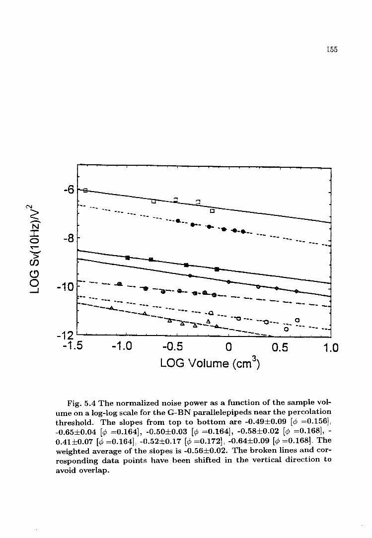
LOG

Sv(

10H

z)/V

155

LOG Volume (cm3)

Fig- 5.4 The normalized noise power as a function of the sample volume on a log-log scale for the G-BN parallelepipeds near the percolation threshold. The slopes from top to bottom are -0.49±0.09 [0 =0.156], -0.65±0.04 [0 =0.164], -0.50±0.03 [0 =0.164], -0.58±0.02 [0 =0.168], - 0.41±0.07 [0 =0.164], -0.52±0.17 [0 =0.172], -0.64±0.09 [0 =0.168], The weighted average of the slopes is -0.56±0.02. The broken lines and corresponding data points have been shifted in the vertical direction to avoid overlap.

156

e for all the G-BN samples used in the sample size experiments can be estimated as

emax= ao/(<fJ - <fJc)!f~ ~10JLm/(0.156-0.150)o.85 ~]mm, which is smaller than and at

the same order of magnitude of the thickness of the samples and the minimum length

and width in decreasing sample volumes. In addition it is obvious (see Section 3.5)

that L > > 1 (measured in the grain size) in the sample size dependent experiments.

Therefore it can be assumed that the samples were approximately three dimensional

and in the region from the crossover (L '" e) to macroscopic homogeneous (L > e).

This implies that (5.2) should correspond to a L -1.68-dependence. However, one could

make the argument that the sample volume was decreased in two dimensions. This

means that Volume ex: L2, which results in a L -1.12-dependence from (5.2). The ar

gument, leading to the value of b = 1.12, is very debatable and suspect, but is given,

because the value of b= 1.12 obtained in this way is very close to the lower bound

obtained from computer simulations on discrete lattice networks in three dimensions

(see the next paragraph). If this were correct it would contrast with the other critical

exponents from the G-BN systems where, as often stated, the values of these critical

exponents are obviously different from the ones for discrete lattices, probably due to

a continuum correction.

These appear to be the first measurements where the size dependence of the 1/ f noise power near the percolation threshold has been obtained experimentally for a

three dimensional percolation continuum system. Computer simulations on the three

dimensional standard discrete percolation networks give a lower and upper bounds of

the exponent b to be -/h = 1.1 and -2{h - 1/11 = 1.26 respectively [Tremblay et

al. 1986]. Therefore the observed exponent b = 1.68 ± 0.06 for the G-BN samples is

much larger than those permissible for discrete lattice networks according to Trem

blay et al. (1986). This fact suggests that the continuum correction in the G-BN

samples could also playa significant role in the size dependence of noise exponent b.

But there are, to the author's best knowledge, no previous experimental result and

existing theoretical model for the exponent b in continuum percolation systems.

The existing predicted values of the noise exponent b are strictly speaking only

157

applicable to conducting samples for which L < ~ [Rammal et al. 1985b]. This

impli~s that the measured value of the noise exponent b would b~ higher if sample is

in the region L > ~. Hence the value of b=1.68 seems quite reasonable because the

G-BN samples, with volume fractions or L > > ~, depending

on <P and the direction. However, these samples could all lie in a transition region

from a fractal character (Sv/V 2 ex: L-b) to a homogeneous one where the Hooge's

law applies (Sv /V 2 ex: L -3). Therefore the observed anomalous size dependence of

Sv /V 2, which deviates from the Hooge's empirical formula, could still be due to the

fractal geometry of the backbone in all the samples (0.156:::; <P :::; 0.172). The value

1.68 of the exponent b is very close to the exponent DB of 1. 74 in three dimensions.

Here the DB is defined as [Chapter 5, Stauffer and Aharony 1994]

(5.3)

where MB is the backbone mass. This could mean that only the mass of graphite on

the backbone gives contributions to the 1/ f noise. This implies that, similar to most

cases where the 1/ f noise is a bulk effect and inversely proportional to the sample vol

ume [Dutta and Horn 1981 and Weissman 1988], the relation Sv /V2 ex: (Volume)-o.56

observed in the G-BN samples could still suggest a bulk source of 1/ f noise on the

backbone.

It has been shown in the previous section that the metal-to-metal (G-G) contacts

on the backbone were possibly responsible for the 1/ f noise in the compacted con

ducting G-BN samples. Therefore, if this is the case, the 1/ f noise and resistance

in the G-BN samples measured come from different mechanisms, both involving the

graphite grains on the backbone. These are intergranular contacts between neigh

bouring graphite grains on the backbone for the former and bulk resistivity for the

later.

The only other experimental study of size effects on the 1/ f noise has been made

158

by Girand et al. (1987) for a two dimensional deterministic fractal lattice. They

measmed the 1/ f noise on a special hierarchical netwo:-k, built from capacitors, with

immeasurable 1/ f noise, and selected carbon layer resistors, all with the same normal

ized noise power. With n=O,1 ,2,3 experimental iterations, they found the exponent

b to be 1, which is half of the value of the exponent b=2 expected from the Hooge's

law for two dimensional Euclidean networks. Moreover, the value of b observed in

this discrete model system is consistent with numerical calculations which gave lower

and upper bounds for the exponent b, in two dimensional lattice percolation models,

of O.97±O.OI and 1.19±O.Ol respectively [Tremblay et al. 1986]. Exact values for the

exponent b for two dimensional continuum percolation systems cannot be obtained

from the above experimental result, because the system studied is a discrete perco

lation network and, as mentioned in the last paragraph, percolation exponents for

a continuum system and for a discrete lattice model can be considerably different.

Therefore, one cannot directly relate these two observed values of the exponent b for

the G-BN system and for the hierarchical network to each other due to their different

dimensionality [two and three dimensions] and characteristics [discrete and contin

uum]. The above hierarchical network study was, nevertheless, an important step in

characterization of size dependence of 1/ f noise in percolation systems.

5.4 Summary

The experimental results for the 1/ f noise in G-BN compressed conducting sam

ples near the percolation threshold have been presented in this chapter. The noise

power spectra were measured in both the axial and transverse directions and have

typical 1/ f behavior. The P- law of the noise power is evidence of the ohmic be

havior of the resistance of the samples and that the noise originates from resistance

fluctuations. The normalized noise powers follow a power-law R1.47 in the axial direc

tion and R1.72 in the transverse direction, where R is the sample DC resistance. These

results can best be explained using a model involving intergranular metal-to-metal

(G-G) contact resistance noise in the Sharvin regime, derived using a self-consistent

159

effective-medium approximation. The most important new result from the 1/ f noise

experiments on the G-BN sample~l is probably the (Volume ).-o.56-dependence of t!le

normalized 1/ f noise magnitude, which applies from near to far from the percolation

threshold on the conducting side. The value of the noise exponent b has been found

to be 1.68±O.04, which is considerably larger than the predictions made for discrete

lattice models.

160

Chapter 6

THE THERMOELECTRIC

POWER

6 .1 Introduction

While the conductivity, dielectric constant and 1/ J noise have been studied exten

sively in percolation systems, the behavior of thermoelectric power near the percola

tion threshold has not been extensively investigated for binary percolation composites.

As mentioned in Section 2.3, Levy and Bergman (1992) proposed a scaling scheme

for the thermoelectric power in percolation systems. Their expressions for the thermo

electric power near the percolation threshold are quite complex and depend in part on

the relation between the electrical and thermal conductivity ratios. In order to obtain

their analytic results, both the ratio (J'i/ (J' c and kif kc must be very small compared to

unity. The physical meaning of these requirements is that the good electrical conduc

tor is also a good thermal conductor and vice versa. Since ki > kc for the graphite

and hexagonal boron nitride, Levy and Bergman's scaling results are not applicable

to the G-BN percolation system. On the experimental side, only one experimental

study on the AI-Ge percolation thin films has been reported and analyzed [Hurvits,

Rosenbaum and McLachlan 1993] following the two theoretical papers [Bergman and

Levy 1991; Levy and Bergman 1992]. As an extension to these previous works, new

power-laws for the thermoelectric powers in binary continuum percolation systems

161

are proposed, and measurements of the thermoelectric power were made on the G

BN parallelepiped samples. T~e new power-laws fo~ the thermoelectric power near

the percolation threshold are developed in Section 6.2. The experimental results for

the thermoelectric power in the G-BN composites are given and analyzed, using the

newly proposed power-laws, in Section 6.3. The thermoelectric data obtained from

the AI-Ge films [ Hurvits et al. 1993] is also re-analyzed in this section. The results

are summarized in Section 6.4.

6.2 New Power-Laws for the Thermoelectric Power

The Milgrom-Shtrikman-Bergman-Levy (MSBL) formula for thermoelectric power

in binary composites is an analytic result [Milgrom and Shtrikman 1989 and Bergman

and Levy 1991] and has previously been used to develop power-laws for thermoelectric

power in percolation systems [Levy and Bergman 1992]. As stated in Subsection

2.3.6, the power-laws proposed by Levy and Bergman are very complex and are not

applicable to the percolation systems in which the electrical insulator is a better

thermal conductor than the another component. In an attempt to improve the Levy

and Bergman's scaling scheme, new power-laws for the thermoelectric power near

the percolation threshold are proposed and will be presented in this section. For

convenience, the MSBL formula is re-written here

Km/Kc _ 1

Sm = Se + (Si - Se) ~ _ 1 ' (6.1 ) Ui/<7c

where the symbols have been defined in Subsection 2.3.6.

To obtain simple and well-defined scaling form for the thermoelectric power in

percolation systems, the terms on the right-hand side of Equation (6.1) have to be

rewritten in the following way

162

(6.2)

where M1(Se,Si, Ke/O"e,I{i/O"i) and M2(Se,Si,Ke/O"e,l{i/O"i), abbreviated as Ml and

M2 respectively, are defined by

(6.3)

(6.4)

For a given set of composites, both Ml and M2 are constant since they depend only

on the electrical and thermal properties of the two components but do not on the

composition of samples. Equation (6.2) shows that the thermoelectric power Sm

of binary composites should be linear function of the ratio of thermal conductivity

and electrical conductivity, i.e. the Wiedeman-Franz ratio Km/O"m and vice versa.

Furthermore, of the three composite variables Sm, J{m and O"m, only two of them are

independent. Equation (6.2) also shows that, at a fixed temperature, the variation

of Sm in binary continuum percolation composites is entirely determined by their

Wiedeman-Franz ratio, which depends on the compositions of sample. Therefore the

problem of how to describe the thermoelectric power in binary continuum percolation

systems can be reduced to how to describe the behavior of the Wiedeman-Franz ratio

in the percolation systems. Before proceeding further in this direction, it is worthy

to recall some fundamental results for the Wiedeman-Franz ratio in homogeneous

materials [Busch and Schade 1976 and references therein]. For homogeneous metals

and at high temperature (T>OD, OD=Debye temperature), the Wiedeman-Franz ratio

vanes as

(6.5)

163

where T is the absolute temperature, and L = 1r32(~)2 = 2.45 X 1O-8(V/k)2 is the

universal Lorenz number. The physical requirement for T>()D is that the relaxation

time must be unchanged when an electrical field and temperature gradient are act

ing, that is, the same scattering processes must be responsible for both the electrical

resistance and the thermal resistance. This condition is satisfied for temperatures

above the Debye temperature, when inelastic scattering is dominant. However, these

considerations do not apply to a semi-metal, such as graphite, where the thermal

conductivity due to the electrons is low compared to that due to the phonons. The

Wiedeman-Franz ratio for an insulator will be defined as Kd Ui, which is a very large

number and is completely unrelated to free electron theory. Note that the Wiedeman

Franz ratio for percolation systems varies drastically with the compositions of samples

as Km and especially U m vary strongly close to the percolation threshold. But there

is, to the author's knowledge, no theoretical model dealing with the ratio Km/um for

binary continuum percolation composites.

In order to use the scaling theory to describe the Wiedeman-Franz ratio near

percolation threshold, consider the case where

Kc Ui - . -, ~ 1 and Ui =I- o. (6.6) U c Iii

Near the percolation threshold and at constant temperature, the Wiedeman-Franz

ratio Km/um is assumed to have the scaling form [Straley 1976, Efros and Shklovskii

1976, and Bergman and Imry 1977J

Km = 1<; I <Pc

for Izl ~ 1, 1

Regime I

Regime II

Regime III

(6.7)

(6.8)

164

The parameters A, B' and A", that appear in (6.8), can only be determined experi

mentally. From the asymptotic forms of A(z), and using the relation (6.2), one can

deduce the following power-laws for the thermoelectric power

for <Pc (6.9)

for <P < <Pc (6.10)

(6.11)

where hI and h2 are two, probably new, critical exponents. Note that the power-laws

(6.9) and (6.10) are similar in form to the percolation equation for the magnetocon

ductivity given in (2.42). This similarity is probably attributed to "two field" coupling

in both these cases: the electrical and external magnetic fields for the magnetocon

ductivity, and the electrical and temperature fields for the thermoelectric power.

Therefore "field coupling" would appear to lead to a difference (off-set), rather than

a directly measured physical quantity, obeying a power-law. One advantage of the

newly proposed percolation equations (power-laws) for thermoelectric power is that

the electrical conductivity and thermal conductivity data for the composites need not

be known or modelled separately when one uses (6.9) and (6.10) to fit the thermo

electric data. It is important to note that the condition (6.6), which is necessary

to use the scaling theory, should apply to the present experimental study of the

graphite and hexagonal boron-nitride composites in which I( and f{c are at the same

order of magnitude, but ui/um «< 1. Note that (6.11) shows that the data for a

system obeying (6.9), (6.10) and (6.11) will go smoothly through the <P = <Pc point, if

f{cui/ f{iuc is not zero.

165

6.3 Experimental Results and Discussion

The thermoelectric power for conducting G-BN parallelepiped samples, with graphite

volume fractions from 0.154 to 0.82, was measured in an evaporation plant at a pres

sure of less than 1 x 10-5 Torr. The sample was mounted between two copper blocks,

of which one was warmed up to 45°C by a heater and the other was cooled down

to 5°C by cold water. Because of the very large resistance of samples on the insu

lating side of the percolation, the thermoelectric power for these samples could not

be measured using the existing instruments. More experimental details are given in

Section 3.6.

The measured thermoelectric power as a function of the graphite volume fraction

is shown in Fig. 6.1, where the solid line is a best fit to the percolation equation

(6.9). From this figure it is observed that the thermoelectric power over a large

range of the graphite volume fractions on the conducting side is nearly constant and

equal to that of <P = 0.82 graphite sample. Very near the percolation threshold,

the thermoelectric power shows a sudden upturn. These results are qualitatively in

good agreement with the predictions made by Webman et al. (1977), using the self

consistent effective-media approximation. The thermoelectric power for the G-BN

samples above the percolation threshold <Pc can be estimated by using the MSBL

formula (6.1). In fact the following approximation holds

(6.12)

Note that Min{I{i, J(c} ~ J(m ~ Max{I{i, J(c} for any binary composites and 1~

J(i/ /{c ~ 10 [Lide 1994] for the G-BN system, so that one has

(6.13)

---~ ........ >

::1. --E en

166

40

20

t~ """"- 0 0 v 0 U - ....

0 0 0.2 0.4 0.6 0.8

Volume fraction 

Fig. 6.1 The thermoelectric power against the volume fraction ¢ for the G-BN parallelepipeds. The solid curve is a best. fit to data, using 0,· =O.150±O.OOl and the power-law (6.9). The best fit parameters are given in the text.

167

On the conducting side, from Fig. 4.2a,

(6.14)

Inserting (6.12), (6.13) and (6.14) into (6.1) or (6.2), one concludes that, to first order,

there is no significant change in Sm on the conducting side for the G-BN system.

As mentioned early in this section, the thermoelectric power data could be fit

ted to the percolation equation (Sm - Mt)cx (fjJ - fjJe)hl. Since only the data on the

conducting side are available, the critical volume fraction fjJe is fixed at 0.lS0±0.00l,

which was obtained from the electrical conductivity data (see Section 4.2), in the

fitting program, while 1~11' pre-factor and exponent hI are allowed to vary to give

the best result. Note that for the G-BN system, MI is equal to the thermoelectric

power of pure graphite sample, according to its definition given in the previous section

and using the approximation (6.12). The best fit values of the parameter Mt, pre

factor and exponent hI are (9.S1±0.01)Jl VI I<, (0.003S±0.001)Jl V II<, and -1.13±0.OS

respectively. The theoretical curve through the data points can thus be written as

Sm = 9.S1 + 0.003S( fjJ - 0.lS0t1.l3. This relation gives the value of Se for graphite

to be 9.S1Jl V I I< in agreement with the measured value on the fjJ=0.82 graphite par

allelepiped of (9.10±0.07)Jl VII<.

In order to test the MSBL equation (6.1), Hurvits, Rosenbaum and McLachlan

(1993) measured the thermoelectric power and electrical conductivity at room tem

perature on the AI-Ge films with varying aluminum volume fractions in the range 0.20

'" 1.0. As the thermal conductivity for the AI-Ge films on glass substrates cannot be

measured experimentally, they used both the GEM equation and another effective

medium equation to calculate the I<m from I<e(AI) and I<i(Ge). Using this data and

the fitted and experimental data for (Jm, (Ji and (Je ((Ji/(Je ~ 10-7), together with a

fixed value of fjJe = 0.S6 obtained from superconducting measurements, they found

that the MSBL formula described their experimental thermoelectric power data rea

sonably well. Shown in Fig. 6.2a is the data of Hurvits et al. (1993) for the AI-Ge

...-:::s:::: -> -J ....... -E Cf)

168

1000r-~--~--~--~--~--~~--~--~--~

750

500

250

q)

0 o~ 00 0

o 0.2 0.4 0.6 0.8 1.0

Volume fraction ~

Fig. 6.2a The thermoelectric power against the volume fraction ¢ for Al - Ge system. The solid curve is a best fit to data, using a fixed ¢c of 0.56 and the power-law (6.9). The experimental data were taken from Hurvits et al. (1993). The best fit parameters are given in the text.

169

system. Since I<i(Ge)/ I<c(Al) ~ 0.12, the Levy and Bergman's power-laws for ther

moelectric power are not applicable to the Al-Ge system. Equation (6.10) can be

fitted to the data, using a fixed ¢c of 0.56. The best fit is Sm=-5.61+4290(0.56-¢)1.90,

which is plotted in Fig. 6.2a. A visual comparison of this fit to that made by Hurvits

et al. (1993) shows that these two best fit theoretical lines are virtually identical.

The advantage of using (6.9) and/or (6.10) is that full details of (J"m(¢) and I<m(¢)

do not have to be known or modelled.

An alternative is to fit the thermoelectric data for the Al-Ge films simultaneously

using equations (6.9) and (6.10), where the critical volume fraction ¢c, the param

eter M I , the prefactors and the two exponents hI and h2 are all allowed to vary

to give a best fit. The two solid curves through the data in Fig. 6.2b show the

best fit. The common parameters in (6.9) and (6.10) are ¢c=0.427±0.001 and MI =

(2.56±0.14)J.lV/ I<. On the conducting side, the exponent hI and pre-factor are found

to be -1.19±0.02 and (0.28±0.04)J.lV/ I< while on the insulating side, h2 and pre-factor

are determined to be -0.7 4±0.01 and (1702±23)J.l V / I<, respectively. In summary,

their thermoelectric power data can also be fitted to the relations Sm =2.56+0.28( ¢-

0.427)-1.19 for ¢ > 0.427 and Sm=2.56+1702(0.427-¢)O.74 for ¢ < 0.427. It is noted

that the apparent critical volume fraction ¢c of 0.427 obtained here is smaller than

that of 0.56 from the electrical conductivity and superconductivity data. This dis

crepancy is qualitatively consistent with computer simulations made by Webman et

al. (1977) and Levy and Bergman (1992), who found that the thermoelectric power

at ¢c, or even slightly smaller than it, is still nearly equal to that of the conducting

component. These results imply that the percolation threshold ¢c, obtained directly

from fitting experimental thermoelectric power data, as given above in this paragraph

, could be smaller than those obtained from the measurements for other percolation

physical properties, such as electrical conductivity.

These measurements of thermoelectric power on the systems G-BN and Al-Ge

seem to be the only experimental studies of the critical behavior of thermoelectric

power in percolation systems. The good agreement between theory and experiment

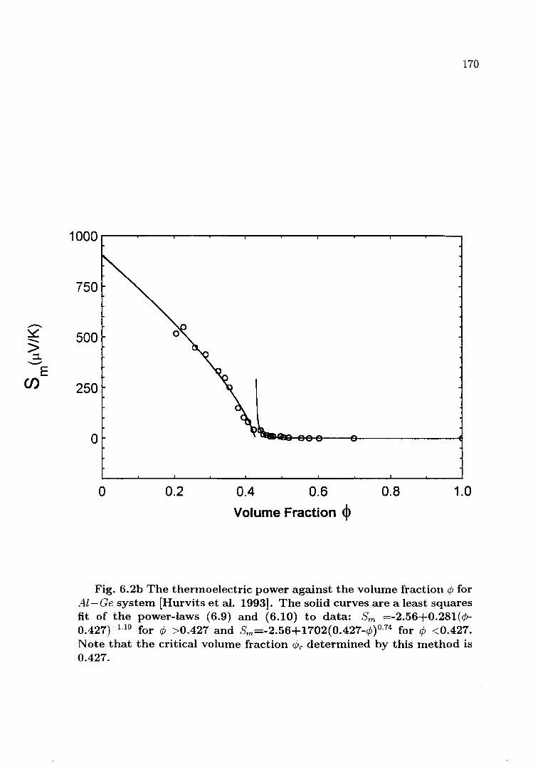
170

750

.-~ 500 ~ --E en 250

o

o 0.2 0.4 0.6 0.8 1.0

Volume Fraction <p

Fig. 6.2b The thermoelectric power against the volume fraction cjJ for Al-Ge system [Hurvits et al. 1993]. The solid curves are a least squares fit of the power-laws (6.9) and (6.10) to data: 8m =-2.56+0.281(ci>-0.427t1.l9 for ci> >0.427 and 8m =-2.56+1702(0.427-ci»o.74 for ci> <0.427. Note that the critical volume fraction cPc determined by this method is 0.427.

171

III both these two cases shows the validity of the two percolation equations (6.9)

and (6.10) derived from the MSBL formula (6.1). However, the two percolation

equations (6.9) and (6.10) for the thermoelectric power on both sides of percolation

threshold, proposed in this thesis, need to be tested by more accurate experimental

investigations, preferably with very good data on both sides of <l>c.

6.4 Summary

Based on the MSBL formula, it has been shown that the thermoelectric power of

binary continuum composites is a linear function of the Wiedeman-Franz ratio. A

scaling scheme for the Wiedeman- Franz ratio near the percolation threshold in bi

nary continuum percolation systems has been proposed. When incorporated into a

modified MSBL formula, this scaling hypothesis results in the two new percolation

equations (power-laws) for the thermoelectric power near and on both sides of the

percolation threshold. The new power-laws for thermoelectric power have a form sim

ilar to the one for the magnetoconductivity, probably due to "two field" coupling in

these two cases. The thermoelectric power data obtained from the G-BN samples on

the conducting side are in accordance with the self-consistent effective-media approx

imation due to Webman et al. (1977), and the MSBL formula. The newly proposed

percolation equations for thermoelectric power can fit the experimental thermoelec

tric data obtained both from the G-BN percolation system and from the AI-Ge one

very well. Levy and Bergman's percolation equations are not suitable for fitting the

data for these two systems.

172

Chapter 7

SUMMARY, CONCLUSION AND

PROPOSALS FOR FUTURE

WORK

The G- BN compressed disc system and powder mixtures undergoing compression

have proved to be very good continuum percolation systems, upon which a number

of typical percolation measurements have been made, and many theoretical percola

tion models have been tested. The various critical exponents measured for the G-BN

systems cannot be explained using a single percolation model.

The critical volume fraction <Pc=0.150 for the G-BN disc samples can be explained

by the existing models [Kusy 1977 and Balberg et al. 1984]. The slightly smaller value

of <Pc ~ 0.12 obtained from the four different types of power experiments (in axial

direction: DC and AC; in transverse direction: DC and AC) are attributed to the

presence of cavities of approximately 7 times the size of the graphite grains. The

conductivity exponents are found to be t = 2.63 and 2.68 in the axial and transverse

directions, respectively, for the disc samples, and t ~ 4.8 and 6.1 in the axial and

transverse directions for both the 50%G-50%BN and 55%G-45%BN powders. As one

can fit the conductivity data with a single conductivity exponent of t=2. 74 over entire

volume fraction range on the conducting side (0.150 '" 0.82), a single metallic con-

173

duct ion mechanism must be responsible to the electrical conduction for all the disc

s"l.mples with cP > cPe. The exponent 5 obtained froT. the conducti vity measurements

on the insulating side does not appear to be related to the dielectric constant expo

nent s. However, the values of exponent 5, which describes the divergence behavior of

conductivity for cP < cPe, are not well understood [Chpater 15, Deutscher et al. (Ed.)

1983].

Close to the percolation threshold it has been observed that the AC conductivity

and dielectric constant vary with frequency as u( cP, w) <X WX and c( cP, w) <X w-y • The

measured exponents x and y for the disc system and two powders are in excellent

agreement with the predictions of intercluster polarization model in spite of the un

usual large values of conductivity exponent t obtained from the DC conductivity data.

Unfortunately, the anomalous -diffusion model cannot be checked quantitatively due

to the lack of knowledge of exponents /J and () for the G-BN systems. The exponent

q, which describes the power-law behavior of the crossover frequency We against the

DC conductivity, has also been measured. On the conducting side, the measured q

values are all less than the predictions of the intercluster polarization model, even

using the observed exponents t and s. Furthermore, the observed values of We for

the powders undergoing compression are several orders of magnitude larger than the

theoretically predicted ones. On the insulating side, the frequency response of the

imaginary part of the AC complex conductivity, W • c( cP, w) against w, collapsed into

a single straight line when normalized by the DC conductivities for the same sample.

This behavior results in a measured We '" 1 and consequently q '" 0, for all the insu

lating samples. This result can not be explained using any of the existing percolation

models and there is no published experimental result available for comparison. The

shallow global minima in the loss tangent tan D as a function of frequency for the in

sulating samples near the percolation threshold are not in agreement with computer

simulations based on the R-C model [Clerc et al. 1990]. These two anomalies cannot

be resolved in this study.

The magneto conductivity exponent tm in a field of lo5T is found to be 3.08. This

174

value is clearly larger than the measured cQnductivity eXPQnent Qf t=2.68. This re

sult contradicts the only existing theQretical mQdel [Bergman 19E'7], which predicts

the same value fQr the cQnductivity eXPQnent t and magnetQcQnductivity eXPQnent

t m. The Qbserved relative magnetQresistivity eXPQnent gc Qf 0.28 is in agreement with

that Qbtained frQm granular percQlatiQn Sn-Ar films [RQhde and Micklitz 1989]. Since

the micrQstructures Qf the G-BN and Sn-Ar are tQPQIQgically very different, the same

magnetQresistivity eXPQnent suggests that the difference between the two. experimen

tal results and the single theQretical predictiQn is a fundamental Qne.

The excess nQise measured in the G-BN cQnducting disc and parallelepiped sam

ples is typically 1/ f"l with the eXPQnent , ranging from 0.98 to. 1.08. Near the

percQlatiQn threshQld the nQrmalized 1/ f nQise PQwer diverges as SV2/V2 ex RW with

eXPQnents w = 1.47 and 1.72 in the axial and transverse directiQns respectively. These

two. eXPQnents are clQse to. the predictiQn Qf a metal-metal CQntact nQise mQdel in the

Sharvin regime and using the self-cQnsistent effective medium apprQximatiQn.

The relatiQn Sv /V2 ex (Volume to.56 fQr the samples near the percQlatiQn thresh

Qld is the first experimental investigatiQn in binary cQntinuum percQlatiQn systems,

and the results CQuid be used to. test the theoretical mQdels develQped by Rammal et

al. (1985b). The nQise eXPQnent b, appeared in the relatiQn Sv /V 2 ex L -b, is fQund

to. be 1.68. This value fQr b is Qutside the estimated range 1.1 '" 1.26, Qbtained frQm

cQmputer simulatiQns Qn three dimensiQnal discrete lattices [Rammal et al. 1985a,

Tremblay et al. 1986].

The thermQelectric PQwer in a binary cQmpQsite has been shQwn to. be a linear

functiQn Qf the Wiedeman-Franz ratio.. A scaling scheme fQr the Wiedeman-Franz ra

tio. in percQlatiQn systems has been prQPQsed in this thesis. This scaling hYPQthesis,

when used in cQnjunctiQn with the MSBL fQrmula, results in two. new PQwer-Iaws fQr

the thermQelectric PQwer, Qne Qn each side Qf the percQlatiQn threshQld. These two.

PQwer-Iaws can be written as (Sm - Mt) ex (<p - <Pc)h1 Qn the cQnducting side Qf the

percQlatiQn and as (Sm - M1) ex (<Pc - <P )-h2 Qn the insulating side. One advantage Qf

175

these two percolation equations is that the electrical conductivity and thermal con

ductivii;y data for the composites 10 not have to be kno'vn separately when one uses

these equations to fit experimental thermoelectric data.

The thermoelectric power data obtained from the G-BN samples with <P ~ <Pc

are in good agreement with predictions based on the self-consistent effective-medium

approximation [Webman et al. 1977J and the MSBL theory. The new power-laws for

thermoelectric power fit the experimental data, obtained from the G-BN percolation

system and from a series of AI-Ge granular films [Hurvits et al. 1993J.

The studies of percolation phenomena associated with the G-BN systems point out

that several investigations still need to be done. For example, on experimental side,

a systematic study of grain size dependence of conductivity exponent t is required as

this dependence has been noted by Chen and Jonhson (1991). This suggestion is mo

tivated and imitated by the investigations carried out by Kusy (1977) and Dovzhenko

and Zhirkov (1995) in which it is found that the critical volume fraction varies with

the ratio of the conducting grain size to the insulating grain size.

As only two experiments on the magnetoconductivity of percolation systems have

been performed up till now, more data, using different percolation systems, is needed

to resolve the fundamental differences between the two observations and the single

theory.

The power-laws for the thermoelectric power in percolation systems, proposed in

this thesis, need to be tested using more and more accurate experimental data.

On the theoretical side, it has been noted in Chapter 5 that, for the Swiss-cheese

model the scaling behavior of the smallest neck width, b cx:( <P - <Pc)'+', determines the

conductivity exponent t and noise exponent w [Halperin et al. ·1985, Garfunkel and

Weissman 1985J. Only two cases, with <p = 1 and 2, have been studied. Neither of

these calculations can explain the t and w values that have been observed in the G-BN

176

systems. Further investigation on the relation between the values of the exponents t

and wand that of the exponent 'P :s needed.

177

Bibliography

[1] Albers A., Ph.D thesis, University of the Witwatersrand (1994).

[2] Alexander S. and Orbach R., J. Physique Lett. (Paris), 43, L625 (1982).

[3] Balberg I. and Bozowski S., Solid St. Commun. 44, 551 (1982).

[4] Balberg I., Anderson C. H., Alexander S. and Wagner N., Phys. Rev. B30, 3933

(1984).

[5] Balberga I., Phys. Rev. Lett. 59, 1305 (1987).

[6] Balbergb I., Phil. Mag. B56, 991 (1987).

[7] Benguigui 1., J. Physque Lett. 46, L-1015 (1985).

[8] Bergman D. J. and Imry Y., Phys. Rev. Lett. 39, 1222 (1977).

[9] Bergman D. J. and Stroud D., Phys. Rev. B32, 6097 (1985).

[10] Bergman D. J., Phil. Mag. B56, 983 (1987).

[ll] Bergman D. J. and Stroud D., in Solid State Physics 46, edited by Ehrenneich

H. and Turnbull D., Academic Press, San Diego (1992).

[12] Bergman D. J. and Levy 0., J. Appl. Phys. 70, 6821 (1991).

[13] Broadbent S. R. and Hammersley J. M., Proc. Camb. Philos. Soc., 53, 629

(1957).

[14] Busch G. and Schade H., Lectures on Solid State Physics, Pergamon (1976).

178

[15] Carmona F., Prudhon P., and Barreau F., Solid St. Commun. 51, 255 (1984).

[16] Chakrabarty R. K., Bardhan K. K. and Basu A., J. Phys.: Condens. Matter 5,

2377 (1993).

[17] Chen C. C. and Chou Y. C., Phys. Rev. Lett. 54, 2529 (1985).

[18] Chen 1. G. and Johnson W. B., J. Mat. Science 26, 1565 (1991).

[19] Chou Y. C. and Jaw T. S. , Solid St. Commun. 67, 753 (1988).

[20] Clarkson M. T. and Smedley S. I., Phys. Rev. A 37, 2070 (1988).

[21] Clerc J. P., Giraud G., Laugier J. M. and Luck J. M., Adv. Phys. 39, 191

(1990).

[22] Dai U., Palevski A. and Deutscher G., Phys. Rev. B36, 790 (1987).

[23] Deprez N. and McLachlan D. S., J. Phys. D.: Appl. Phys. 21, 101 (1988).

[24] Deptuck D., Harrison J. P. and Zawadski P., Phys. Rev. Lett. 54, 913 (1985).

[25] Deutscher G. and Rappaport M. L., J. Phys. Lett. (Paris) 40, L219 (1979).

[26] Deutscher G., Zallen R. and Adler J. (editors), Percolation Structures and Pro

cesses, Annals of the Israel Physical Society, Vo1.5 (1983).

[27] Dovzhenko A. Y. and Zhirkov P.V., Phys. Lett. A204, 247 (1995).

[28] Dutta P. and Horn P. M., Rev. Mod. Phys. 53, 497 (1981).

[29] Efros A. 1. and Shklovskii B. I., Phys. Stat. Sol. (b) 76, 475 (1976).

[30] Essam J. W., Rep. Prog. Phys., 43,833 (1980).

[31] Feng S., Halperin B. I. and Sen P. N., Phys. Rev. B35, 197 (1987).

[32] Fisher M.E., Physics, 3, 255 (1961).

[33] Fitzpatrick J. P., Malt R. B. and Spaepen F., Phys. Lett. A47, 207 (1974).

179

[34] Fizazi A., Moulton J., Pakbaz K., Rughooputh S. D. D. V., Smith P. and Heeger

A. J., Phys. Rev. Lett. 64, 2180 (1990).

[35] Frisch H. 1. and Hammersley J. M., J. Soc. Indust. Appl. Math. 11,894 (1963).

[36] Garfunkel G. A. and Weissman M. B., Phys. Rev. Lett. 55, 296 (1985).

[37] Gefen Y., Aharony A. and Alexander S., Phys. Rev. Lett. 50, 77 (1983).

[38] Girand G., Clerc J. P., Orsal B. and Laugier J. M., Europhys. Lett. 3(8), 935

(1987).

[39] Grannan D. M., Garland J. C. and Tanner D. B., Phys. Rev. Lett. 46, 375

(1981 ).

[40] Grave 1., Deutscher G. and Alexander S., Phys. Rev. Lett. 48, 1497 (1982).

[41] Halperin B. 1., Feng S. and Sen P. N., Phys. Rev. Lett. 54, 2391 (1985).

[42] Harris A. B., Phys. Rev. B28, 2614 (1983).

[43] Herring C., J. Appl. Phys. 31, 1939 (1960).

[44] Hooge F. N., Phys. Lett. A29, 139 (1969).

[45] Hooge F. N., Kleinpenning T. G. M. and Vandamme 1. K. J., Rep. Prog. Phys.,

44, 480 (1981).

[46] Hundley M. F. and Zettl A., Phys. Rev. B38, 10290 (1988).

[47] Hurvits G., Rosenbaum R. and McLachlan D. S., J. Appl. Phys. 73, 7441 (1993).

[48] Kang W. N., Kim D. H., Park J. H., Hahn T. S., Choi S. S. and Gray K. E.,

Physica C233, 402 (1994).

[49] Kirkpatrick S., Rev. Mod. Phys. 45, 574 (1973).

180

[50] Kirkpatrick S., in Proceedings of Les Houches Summer School on Ill-Condensed

Matter (edited cy B3.lian R., Maynard R. and Toulolse G.), North-Holland,

Amsterdam (1979).

[51] Koch R. H., Laibowitz R. B., Alessandrini E. I. and Viggiano J. M., Phys. Rev.

B32, 6932 (1985).

[52] Kogut P. M. and Straley J. P., J. Phys. C.: Solid State Phys. 12,2151 (1979).

[53] Kolek A. and Kusy A., Phys. Rev. B43, 11274 (1991).

[54] Kusy R. P., J. Appl. Phys. 48, 5301 (1977).

[55] Laibowitz R. B. and Gefen Y., Phys. Rev. Lett. 53, 380 (1984).

[56] Laugier J. M., These de Troisieme cycle, Universite de Provence, Marseille

(1982).

[57] Laugier J. M., These d'Etat, Universite de Provence, Marseille (1987).

[58] Laugier J. M., Clerc J. P. and Girand G., in Proceedings of International AMSE

Conference, edited by Mesnard G., Lyon: AMSE (1986).

[59] Lee J.-W., See S. K., Kim J.-J. and Kim H. C., J. Korean Phys. Soc. 26,683

(1993).

[60] Lee S., Song Y., Noh T., Chen X. and Gaines J. R., Phys. Rev. B34, 6719

(1986).

[61] Leeman C., Skove M. J. and Stillwell E. P., Solid State Commun. 35, 97 (1980).

[62] Levinshtein M. E., Shur M. S. and Efros A. 1., Zh. Eksp. Teor. Fiz. 69,

2203(1975)(Sov. Phys. -JETP, 42, 1120 (1976)).

[63] Levy O. and Bergman D. J., J. Phys. A: Math. Gen. 25, 1875 (1992).

[64] Lide D. R. (editor-in-chief), CRC Handbook of Chemistry and Physics, CRC

Press (1994).

181

[65] Lin J. J., Phys. Rev. B44, 789 (1991).

[66] Lynch R. W. and Drickamer H. G., J. Chern. Phys. 44, 181 (1966).

[67] Malliaris A. and Turner D. T., J. Appl. Phys. 42,614 (1971).

[68] Mantese J. V., Curtin W. A. and Webb W. W. Phys. Rev. B33, 7897 (1986).

[69] Mantese J. V. and Webb W. W., Phys. Rev. Lett. 55,2212 (1985).

[70] McLachlan D. S., J. Phys. C19, 1339 (1986).

[71] McLachlan D. S., Electrically Based Microstructural Characterization, edited

by Gerhardt R. A., Taylor S. R., and Garboczi E. J., MRS Proceedings 411

(1996).

[72] McLachlan D. S., Blaskiewicz M. and Newnham R. E., J. Am. Ceram. Soc. 73,

2187 (1990).

[73] McLachlan D. S., J. Appl. Phys. 70, 3681 (1991).

[74] Michels M. A. J., Brokken-Zijp J. C. M., Groenewoud W. M. and Knoester A.,

Physica A 157, 529 (1989).

[75] Milgrom M. and Shtrikman S., Phys. Rev. Lett. 62, 1979 (1989).

[76] Moha-Ouchane M., Peyrelasse J. and Boned C., Phys. Rev. A 35, 3027 (1987).

[77] Nan Ce-Wen, Prog. in Mat. Science 37,1 (1993).

[78] Nitsch K., Dziedzic A. and Golonka 1., lnt. J. Electronics 69, 515 (1990).

[79] Octavio M., Gutierrez G. and Aponte J., Phys. Rev. B36, 2461 (1987).

[80] Peyrelasse J., Moha-Ouchane M. and Boned C., Phys. Rev. A38, 904 (1988).

[81] Pierre C., Deltour R., Van Bentum J., Perenboom J. A. A. J. and Rammal R.,

Phys. Rev. B42, 3386 (1990).

182

[82] Pike G. E., in Electrical Transport and Optical Properties of Imhomogeneous

Media, Edited by GarlaI'd J. C. and Tanner D. B., AlP Conf. Proc. 40, 356

(1978).

[83] Putley E. H., The Hall Effect and Related Phenomena, Butterworths, London

(1960).

[84] Rajab M. and Coleman D. S., Powder Metall. 28, 207 (1985).

[85] Rammal R. and Toulouse G., ibid, 44, L13 (1983).

[86] Rammal R., Phys. Rev. Lett. 55, 1428 (1985).

[87] Rammala R., Tannous C., Breton P. and Tremblay A. M. S., Phys. Rev. Lett.

54, 1718 (1985).

[88] Rammalb R., Tannous C. and Tremblay A. M. S., Phys. Rev. A31, 2662 (1985).

[89] Reynolds W. N., Physical Properties of Graphite, Elsevier Materials Science

Series (1968).

[90] Rohde M. and Micklitz H., Physica A157, 120 (1989).

[91] Rudman D. A., Caladreze J. J. and Garland J. C., Phys. Rev. B33, 1456 (1986).

[92] Scher H. and Zallen R., J. Chern. Phys. 53, 3759 (1970).

[93] Schirmacher W., J. Phys. A: Math. Gen. 27, L727 (1994).

[94] Skal A. S. and Shklovskii B.I., Fiz. Tekh. Poluprov., 8, 1586(1974)( Sov. Phys.

Semicond., 8, 1029 (1975)).

[95] Smilauer P., Contemporary Physics, 32,89 (1991).

[96] Song Y., Lee S.-I. and Gaines J. R., Phys. Rev. B46, 14 (1992).

[97] Song Y., Misra A., Cao Y. Querubin A., Chen Xiao-Deng, Crooker P. P. and

Gaines J. R., Physica C172, 1 (1990).

183

[98] Song Y., Noh T. W., Lee S. 1. and Gaines J. R., Phys. Rev. B33, 904 (1986).

[99] Stauffer D. S. and Aharony A., Introduction to Percolation Theory, 2nd Ed.,

Taylor and Francis (1994).

[100] Stephen M. J., Phys. Rev. B17, 4444 (1978).

[101] Straley J. P., J. Phys. C: Solid St. Phys. 9, 783 (1976).

[102] Straley J. P., Phys. Rev. B15, 5733 (1977).

[103] Straley J. P., J. Phys. C: Solid St. Phys. 13, L773 (1980).

[104] Straley J. P., J. Phys. D14, 2101 (1981).

[105] Stroud D. and Bergman D. J., Phys. Rev. B25, 2061 (1982).

[106] Takagi K., Mizunami T., Suzuki J. I. and Masuda S., IEEE Trans. Components,

Hybrids, Manuf. Technol., Vol. CHMT-9, 141 (1986).

[107] Testa J. A., Song Y., Chen X. D., Golben J., Lee S. 1., Patton B. R. and Gaines

J. R., Phys. Rev. B38, 2922 (1988).

[108] Tremblay A. M. S., Feng S. and Breton P., Phys. Rev. B33, 2077 (1986).

[109] Tremblay A. M. S., Fourcade B. and Breton P., Physica A157, 89 (1989).

[110] Van Dijk M. A., Phys. Rev. Lett., 55, 1003 (1985).

[111] Van Dijk M. A., Casteleijn G., Joosten J. G. H., and Levine Y. K., J. Chern.

Phys. 85, 626 (1986).

[112] Vandamme 1. K. J., IEEE Trans. Components, Hybrids, Manuf. Technol., Vol.

CHMT-10, 290 (1987).

[113] Webman 1., Jortner J. and Cohen M. H., Phys. Rev. B16, 2959 (1977).

[114] Webman I., Phys. Rev. Lett. 47, 1496 (1981).

[115] Weissman M. B., Rev. Mod. Phys. 60, 537 (1988).

[116] Wilkinson D., Langer J. S. and Sen P. N., Phys. Rev. B28, 1081 (1983).

[117] Williams J. 1. and Burdett R. K., J. Phys. C 2, 298 (1969).

[118] Yoon S. and Lee S.-I., Physica B167, 133 (1990).

[119] Zallen R., The Physics of Amorphous Solids, Wiley, New York (1983).

184

the conductivity, dielectric constant, …

Documents