the design and use of the icru/aapm ct radiation dosimetry … · 2020-02-14 · the design and use...

AAPM REPORT NO. 200

The Design and Use of the ICRU/AAPM CT Radiation Dosimetry Phantom:

An Implementation of AAPM Report 111

The Report of AAPMTask Group 200

January 2020

DISCLAIMER: This publication is based on sourcesand information believed to be reliable, but theAAPM, the authors, and the editors disclaim any war-ranty or liability based on or relating to the contents ofthis publication.

The AAPM does not endorse any products, manufac-turers, or suppliers. Nothing in this publication shouldbe interpreted as implying such endorsement.

© 2020 by American Association of Physicists in Medicine

This page intentionally left blank.

The Design and Use of the ICRU/AAPMCT Radiation Dosimetry Phantom:

An Implementation of AAPM Report 111

The Report of AAPM Task Group 200

Donovan M. Bakalyar1, Chair, Erin Angel2, Kirsten Lee Boedeker3, John Boone4,

Kish Chakrabarti5, Huaiyu Heather Chen-Mayer6, Dianna Cody7, Robert Dixon8,

Sue Edyvean9, Wenzheng Feng10, Shuai Leng11, Sarah McKenney12,

Michael McNitt-Gray13, Richard Morin14, J. Thomas (Tom) Payne15,

Robert Pizzutiello16, Jeffrey Siewerdsen17,

Keith Strauss18, and Paul Sunde19

Additional Contributors:

Lars Herrnsdorf, Marcus Söderberg, Rob Morrison,

Elisabeth Nilsson, and George W. Burkett

1Henry Ford Health System, Detroit, MI2Canon Medical Systems, Tustin, CA3Canon Medical Systems, Los Angeles, CA4University of California–Davis Medical Center, Sacramento, CA5CDRH/FDA, Silver Spring, MD6NIST, Gaithersburg, MD7University of Texas MD Anderson Cancer Center, Houston, TX8Wake Forest University, Winston-Salem, NC9Centre for Radiation, Chemical and Environmental Hazards (CRCE), Chilton, Oxfordshire, UK10Saint Barnabas Medical Center, Livingston, NJ11Mayo Clinic, Rochester, MN12Stanford University, Stanford, CA13David Geffen School of Medicine at UCLA, Los Angeles, CA14Mayo Clinic, Jacksonville, FL15Midwest Radiation Consultants, Inc., Ora Valley, AZ16Upstate Medical Physics (retired), Victor, NY17Johns Hopkins University, Baltimore, MD18Children’s Hospital Medical Center, Cincinnati, OH19Radcal Corporation, Monrovia, CA

DISCLAIMER: This publication is based on sources and information believed to be reliable,but the AAPM, the authors, and the publisher disclaim any warranty or liability

based on or relating to the contents of this publication.

The AAPM does not endorse any products, manufacturers, or suppliers. Nothing in thispublication should be interpreted as implying such endorsement.

ISBN: 978-1-936366-74-3ISSN: 0271-7344

© 2020 by American Association of Physicists in Medicine

All rights reserved

Published by

American Association of Physicists in Medicine1631 Prince Street

Alexandria, VA 22314

THE REPORT OF AAPM TASK GROUP 200:The Design and Use of the ICRU/AAPM CT Radiation Dosimetry Phantom: An Implementation of AAPM Report 111

5

Contents

1. Background and Rationale . . . . . . . . . . . . . . . . . . . . . . . . . . . . . . . . . . . . . . . . . . . 6

2. Glossary . . . . . . . . . . . . . . . . . . . . . . . . . . . . . . . . . . . . . . . . . . . . . . . . . . . . . . . . . . 6

3. Description of the ICRU/AAPM Phantom . . . . . . . . . . . . . . . . . . . . . . . . . . . . . . 73.1 Assembly of the Phantom . . . . . . . . . . . . . . . . . . . . . . . . . . . . . . . . . . . . . . . . . . . . . . . . . . . . . . . . . . . . . 93.2 Alignment of the Phantom on the Table . . . . . . . . . . . . . . . . . . . . . . . . . . . . . . . . . . . . . . . . . . . . . . . . . . 9

4. Measurement Methodology . . . . . . . . . . . . . . . . . . . . . . . . . . . . . . . . . . . . . . . . . 104.1 Background. . . . . . . . . . . . . . . . . . . . . . . . . . . . . . . . . . . . . . . . . . . . . . . . . . . . . . . . . . . . . . . . . . . . . . . . 104.2 Determining Deq and H(L) . . . . . . . . . . . . . . . . . . . . . . . . . . . . . . . . . . . . . . . . . . . . . . . . . . . . . . . . . . . . 114.3 An Example Using Real-Time Data Acquisition . . . . . . . . . . . . . . . . . . . . . . . . . . . . . . . . . . . . . . . . . . . 11

4.3.1 Using Real-Time Dose Measurements along the Axis . . . . . . . . . . . . . . . . . . . . . . . . . . . . . . . . 124.3.2 Using Real-Time Dose Measurements near the Periphery . . . . . . . . . . . . . . . . . . . . . . . . . . . . 124.3.3 Choosing Scanning Parameters for the Peripheral Dose Profile . . . . . . . . . . . . . . . . . . . . . . . . 144.3.4 Determining h(L) for Small Values of L . . . . . . . . . . . . . . . . . . . . . . . . . . . . . . . . . . . . . . . . . . . . 15

5. Step-by-Step Procedure for Measurements on the Phantom . . . . . . . . . . . . . . 155.1 Data Acquisition, Single Scan Method . . . . . . . . . . . . . . . . . . . . . . . . . . . . . . . . . . . . . . . . . . . . . . . . . . . 155.2 Data Acquisition, Serial Method . . . . . . . . . . . . . . . . . . . . . . . . . . . . . . . . . . . . . . . . . . . . . . . . . . . . . . . 165.3 Additional Collimations and Pitch Values . . . . . . . . . . . . . . . . . . . . . . . . . . . . . . . . . . . . . . . . . . . . . . . . 165.4 Data Analysis . . . . . . . . . . . . . . . . . . . . . . . . . . . . . . . . . . . . . . . . . . . . . . . . . . . . . . . . . . . . . . . . . . . . . . 165.5 Comparison to CTDI100 Measurements . . . . . . . . . . . . . . . . . . . . . . . . . . . . . . . . . . . . . . . . . . . . . . . . . 17

6. Practical Implementation of the Measurement Methodology . . . . . . . . . . . . . 186.1 Measurements in the Full (3 Sections, 60 cm Length) Phantom. . . . . . . . . . . . . . . . . . . . . . . . . . . . . . . 186.2 Measurements in a Single Section of the ICRU/AAPM Phantom . . . . . . . . . . . . . . . . . . . . . . . . . . . . . . 186.3 Measurements in Air . . . . . . . . . . . . . . . . . . . . . . . . . . . . . . . . . . . . . . . . . . . . . . . . . . . . . . . . . . . . . . . . 186.4 Measurements in Very Wide Beams and Using Stationary Tables . . . . . . . . . . . . . . . . . . . . . . . . . . . . . 20

7. Conclusions . . . . . . . . . . . . . . . . . . . . . . . . . . . . . . . . . . . . . . . . . . . . . . . . . . . . . . 21

8. References . . . . . . . . . . . . . . . . . . . . . . . . . . . . . . . . . . . . . . . . . . . . . . . . . . . . . . . 21

Appendix 1: Measurements in Other Geometries . . . . . . . . . . . . . . . . . . . . . . . . . . . 23

Appendix 2: Measurement Equipment Note . . . . . . . . . . . . . . . . . . . . . . . . . . . . . . . 24

Appendix 3: Supplemental Material Available . . . . . . . . . . . . . . . . . . . . . . . . . . . . . . 25Data Recording . . . . . . . . . . . . . . . . . . . . . . . . . . . . . . . . . . . . . . . . . . . . . . . . . . . . . . . . . . . . . . . . . . . . . . . . . . 25Animations . . . . . . . . . . . . . . . . . . . . . . . . . . . . . . . . . . . . . . . . . . . . . . . . . . . . . . . . . . . . . . . . . . . . . . . . . . . . . 25Tutorial and Example for Fine-Tuning the Determination of Deq . . . . . . . . . . . . . . . . . . . . . . . . . . . . . . . . . . . . 25Machine Drawings for Phantom . . . . . . . . . . . . . . . . . . . . . . . . . . . . . . . . . . . . . . . . . . . . . . . . . . . . . . . . . . . . . 25

Appendix 4: Corresponding Human Size using Water-Equivalent Diameter . . . . . 33

Appendix 5: Fine Tuning Deq . . . . . . . . . . . . . . . . . . . . . . . . . . . . . . . . . . . . . . . . . . . . . 35


6

1. Background and Rationale

Although the CTDI phantom and its associated pencil ionization chamber measurement methodologyhave proven to be very useful, they suffer from limitations that have been critically examined over thepast several years. As a consequence, Task Group 111 was formed by the AAPM to address some ofthe concerns that had been raised. Among these concerns are the following:

1. CTDI100 is a surrogate for the dose at the center of a scan of a single, fixed length, 100 mm, and excludes the dose that would accumulate for longer scans. “This underestimation is systematic, applying to narrow and wide beams alike, and slowly becomes larger with increasing width of the z-axis collimation.”1

2. Some scanners employ very wide beams, approaching or even wider than the length of the 100 mm pencil chamber, rendering the CTDI paradigm completely unsuitable for characterizing the dose.

3. CTDI may be inappropriate for stationary table applications, particularly for beams wider than 100 mm. AAPM Report 1111 offered several recommendations for a new measurement methodology and suggested several phantom designs.

Task Group 200 and the ICRU’s Committee on Radiation Dose and Image-Quality Assessment inComputed Tomography have jointly developed a phantom design and robust measurement schemesthat follow the methodology of AAPM Report 111 and are suitable for a wide range of CT scannerdesigns and scanning conditions. Several prototype phantoms were built by a research group at theUniversity of California–Davis (UC Davis), and these phantoms have been tested at several centersaround the United States as well as in England.

The purpose of this current report is to (a) describe the design of the phantom and (b) suggest abroadly applicable measurement methodology that overcomes the limitations of CTDI100 and the met-rics derived from it, such as CTDIvol. The resulting measurement procedures have been developed forconventional MDCT scanners, including models with wide (16 cm, for example) beams. However, theapplication of this methodology to flat panel and specialized cone-beam CT systems presents specialchallenges that are briefly discussed in Appendix 1. The solutions to these particular problems arebeyond the scope of this report.

2. Glossary

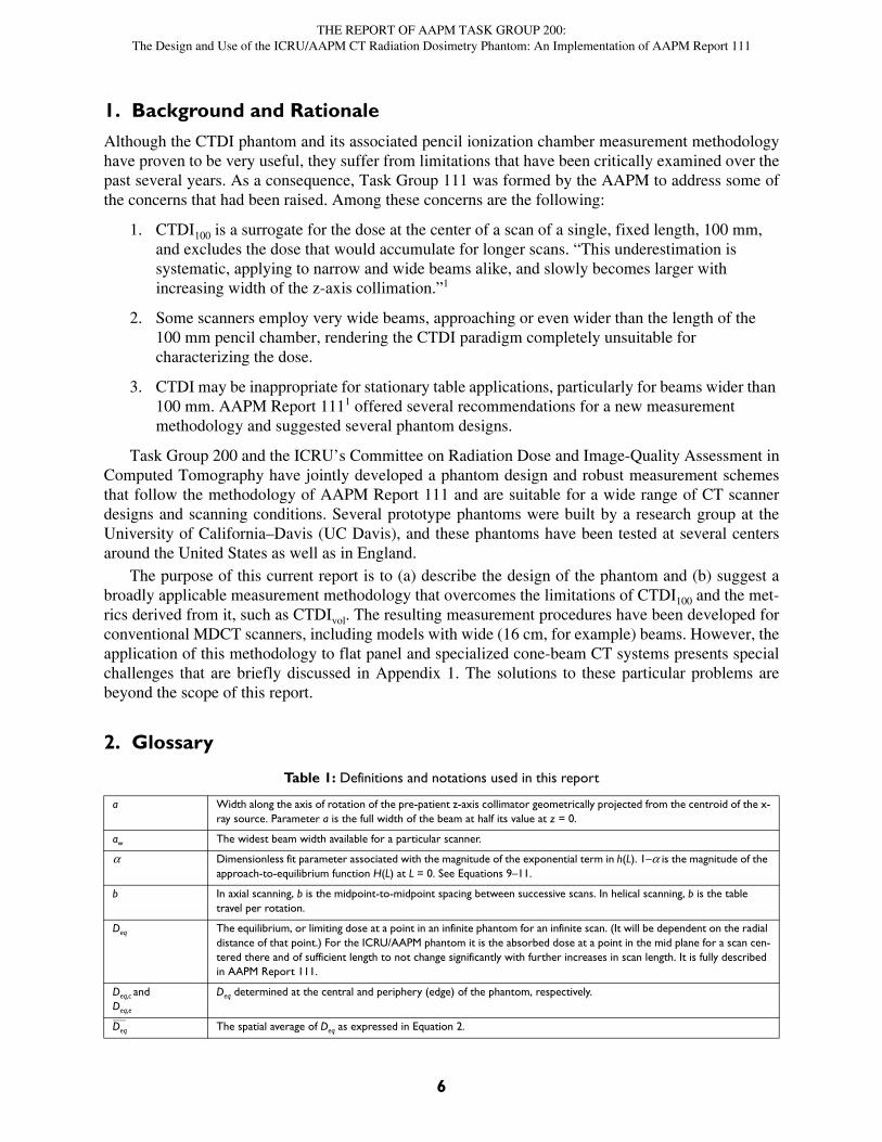
Table 1: Definitions and notations used in this report

a Width along the axis of rotation of the pre-patient z-axis collimator geometrically projected from the centroid of the x-ray source. Parameter a is the full width of the beam at half its value at z = 0.

aw The widest beam width available for a particular scanner.

Dimensionless fit parameter associated with the magnitude of the exponential term in h(L). 1– is the magnitude of the approach-to-equilibrium function H(L) at L = 0. See Equations 9–11.

b In axial scanning, b is the midpoint-to-midpoint spacing between successive scans. In helical scanning, b is the table travel per rotation.

Deq The equilibrium, or limiting dose at a point in an infinite phantom for an infinite scan. (It will be dependent on the radial distance of that point.) For the ICRU/AAPM phantom it is the absorbed dose at a point in the mid plane for a scan cen-tered there and of sufficient length to not change significantly with further increases in scan length. It is fully described in AAPM Report 111.

Deq,c andDeq,e

Deq determined at the central and periphery (edge) of the phantom, respectively.

Deq The spatial average of Deq as expressed in Equation 2.


7

3. Description of the ICRU/AAPM Phantom

The assembled ICRU/AAPM phantom is shown in Figure 1. It can be divided into three sections tomake it more manageable. When assembled, the three sections form a cylinder 30 cm in diameter and60 cm in length. The phantom is made of high-density (0.97 g/cm3) polyethylene, which was selectedbecause it is (a) relatively light in weight, (b) closely mimics the absorption properties of human adi-pose tissue, and (c) is readily available and relatively inexpensive. In addition, at the particular diame-ter of 30 cm, Monte Carlo calculations show that the dose in-medium (as opposed to the air kerma) atthe phantom’s center is nearly the same as it would be for a water phantom of the same diameter.1

Each of the three sections has a mass of around 13.7 kg (weighing about the same as a fullyassembled 32-cm CTDI phantom). Thus, when assembled, the total mass is 41.1 kg (around 91 lb).Channels, parallel to the cylinder axis, are bored deep into the phantom so that a radiation dosimetercan be positioned within the central transverse plane of the phantom, as shown in Figure 1.

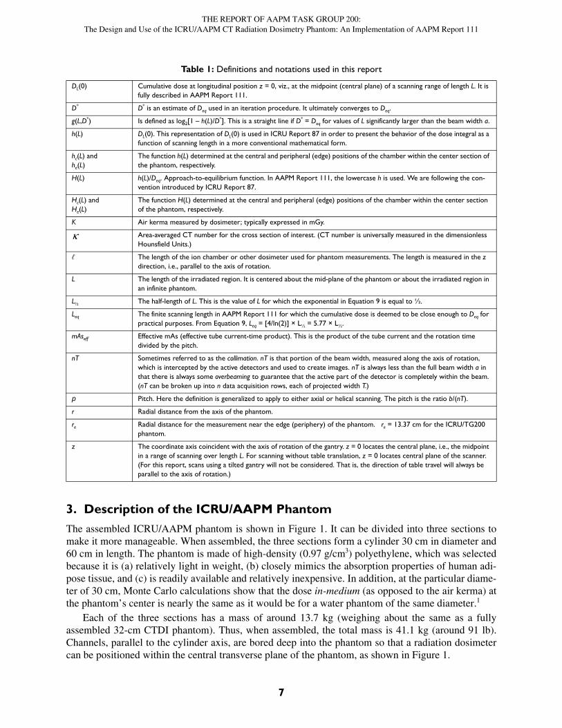
DL(0) Cumulative dose at longitudinal position z = 0, viz., at the midpoint (central plane) of a scanning range of length L. It is fully described in AAPM Report 111.

D* D* is an estimate of Deq used in an iteration procedure. It ultimately converges to Deq.

g(L,D*) Is defined as log2[1 – h(L)/D*]. This is a straight line if D* = Deq for values of L significantly larger than the beam width a.

h(L) DL(0). This representation of DL(0) is used in ICRU Report 87 in order to present the behavior of the dose integral as a function of scanning length in a more conventional mathematical form.

hc(L) andhe(L)

The function h(L) determined at the central and peripheral (edge) positions of the chamber within the center section of the phantom, respectively.

H(L) h(L)/Deq. Approach-to-equilibrium function. In AAPM Report 111, the lowercase h is used. We are following the con-vention introduced by ICRU Report 87.

Hc(L) andHe(L)

The function H(L) determined at the central and peripheral (edge) positions of the chamber within the center section of the phantom, respectively.

K Air kerma measured by dosimeter; typically expressed in mGy.

Area-averaged CT number for the cross section of interest. (CT number is universally measured in the dimensionless Hounsfield Units.)

ℓ The length of the ion chamber or other dosimeter used for phantom measurements. The length is measured in the z direction, i.e., parallel to the axis of rotation.

L The length of the irradiated region. It is centered about the mid-plane of the phantom or about the irradiated region in an infinite phantom.

L½ The half-length of L. This is the value of L for which the exponential in Equation 9 is equal to ½.

Leq The finite scanning length in AAPM Report 111 for which the cumulative dose is deemed to be close enough to Deq for practical purposes. From Equation 9, Leq = [4/ln(2)] × L½ = 5.77 × L½.

mAseff Effective mAs (effective tube current-time product). This is the product of the tube current and the rotation time divided by the pitch.

nT Sometimes referred to as the collimation. nT is that portion of the beam width, measured along the axis of rotation, which is intercepted by the active detectors and used to create images. nT is always less than the full beam width a in that there is always some overbeaming to guarantee that the active part of the detector is completely within the beam. (nT can be broken up into n data acquisition rows, each of projected width T.)

p Pitch. Here the definition is generalized to apply to either axial or helical scanning. The pitch is the ratio b/(nT).

r Radial distance from the axis of the phantom.

re Radial distance for the measurement near the edge (periphery) of the phantom. re = 13.37 cm for the ICRU/TG200 phantom.

z The coordinate axis coincident with the axis of rotation of the gantry. z = 0 locates the central plane, i.e., the midpoint in a range of scanning over length L. For scanning without table translation, z = 0 locates central plane of the scanner. (For this report, scans using a tilted gantry will not be considered. That is, the direction of table travel will always be parallel to the axis of rotation.)

Table 1: Definitions and notations used in this report


8

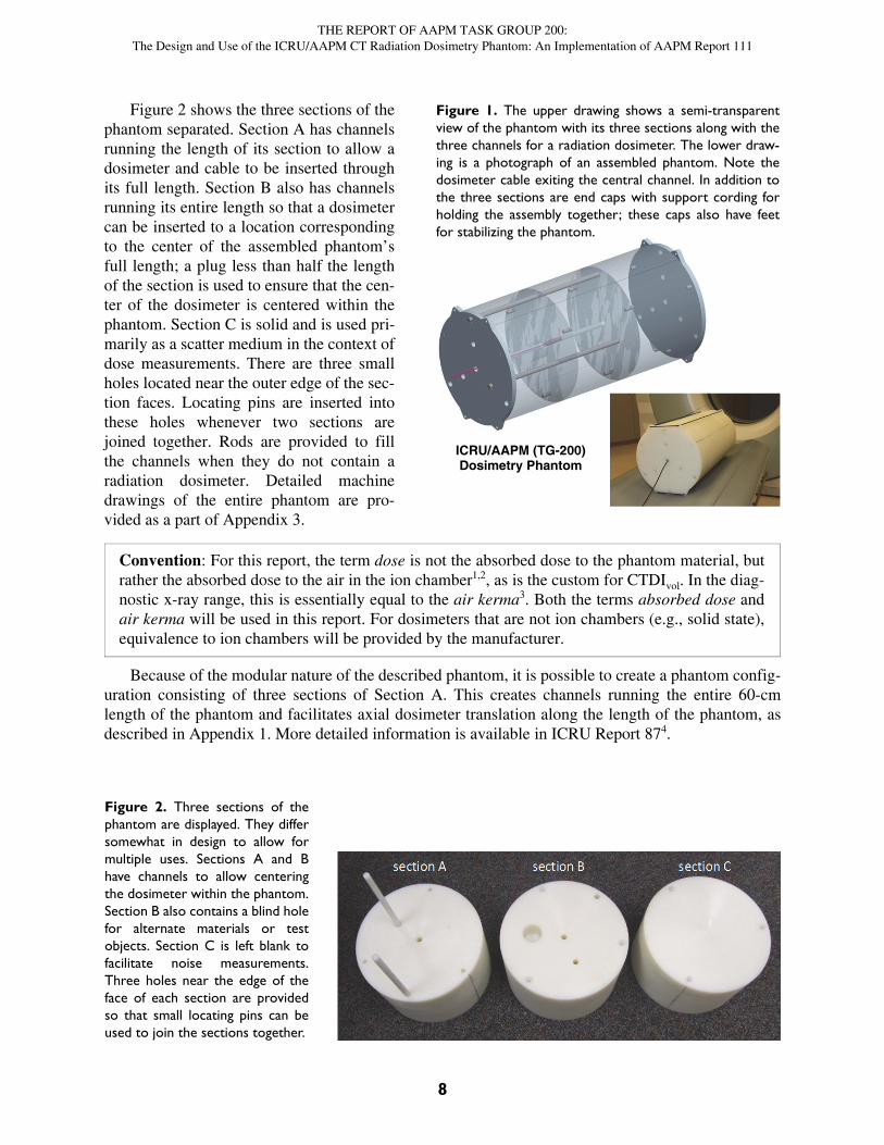
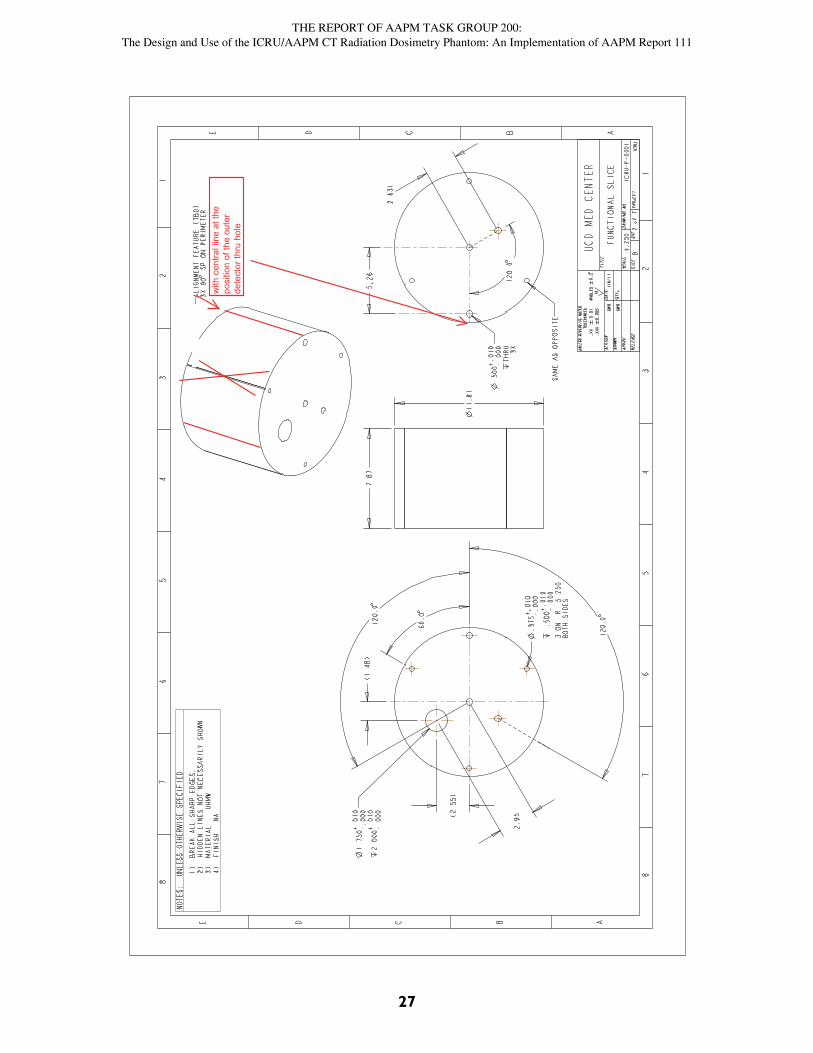
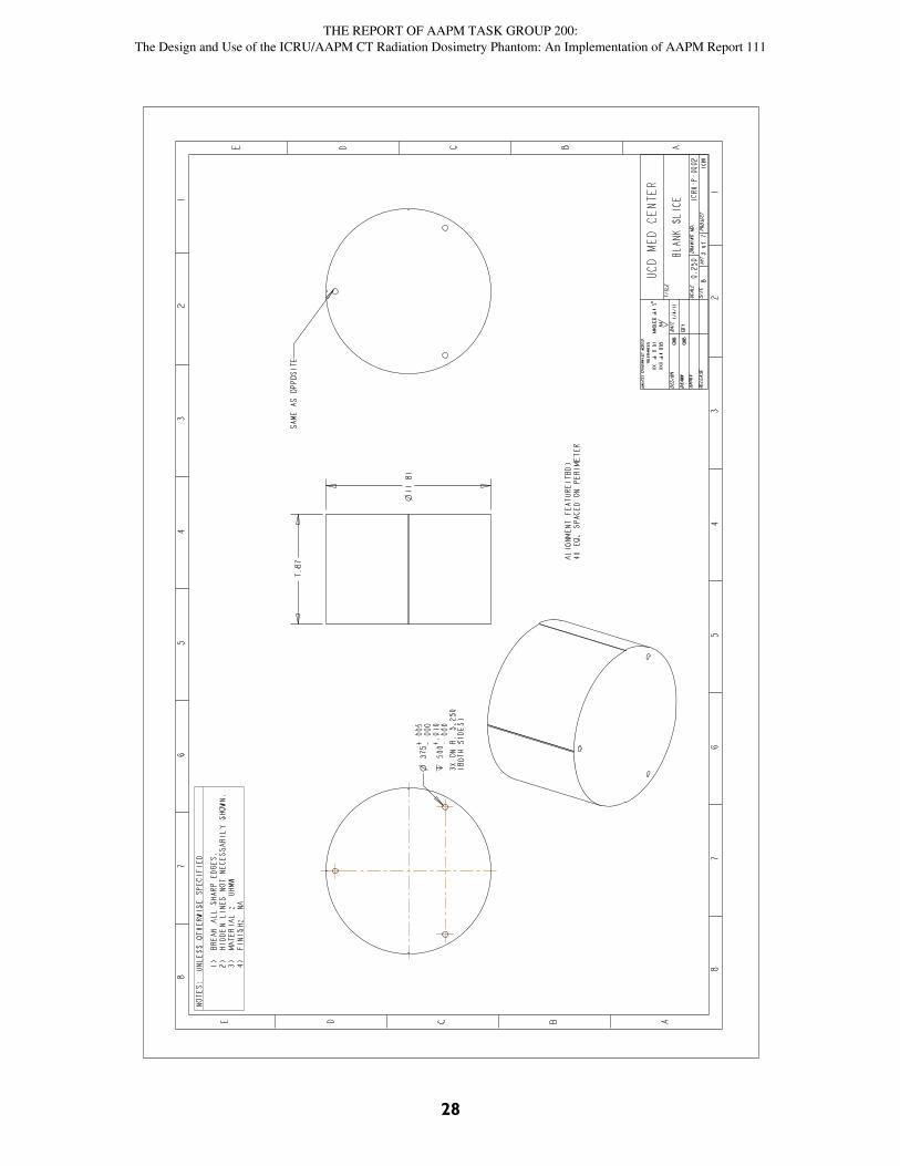
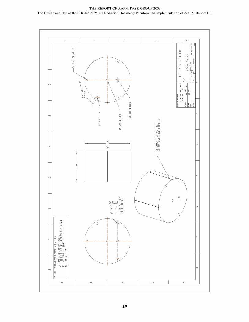
Figure 2 shows the three sections of thephantom separated. Section A has channelsrunning the length of its section to allow adosimeter and cable to be inserted throughits full length. Section B also has channelsrunning its entire length so that a dosimetercan be inserted to a location correspondingto the center of the assembled phantom’sfull length; a plug less than half the lengthof the section is used to ensure that the cen-ter of the dosimeter is centered within thephantom. Section C is solid and is used pri-marily as a scatter medium in the context ofdose measurements. There are three smallholes located near the outer edge of the sec-tion faces. Locating pins are inserted intothese holes whenever two sections arejoined together. Rods are provided to fillthe channels when they do not contain aradiation dosimeter. Detailed machinedrawings of the entire phantom are pro-vided as a part of Appendix 3.

.

Because of the modular nature of the described phantom, it is possible to create a phantom config-uration consisting of three sections of Section A. This creates channels running the entire 60-cmlength of the phantom and facilitates axial dosimeter translation along the length of the phantom, asdescribed in Appendix 1. More detailed information is available in ICRU Report 874.

Figure 1. The upper drawing shows a semi-transparentview of the phantom with its three sections along with thethree channels for a radiation dosimeter. The lower draw-ing is a photograph of an assembled phantom. Note thedosimeter cable exiting the central channel. In addition tothe three sections are end caps with support cording forholding the assembly together; these caps also have feetfor stabilizing the phantom.

ICRU/AAPM (TG-200)Dosimetry Phantom

Convention: For this report, the term dose is not the absorbed dose to the phantom material, butrather the absorbed dose to the air in the ion chamber1,2, as is the custom for CTDIvol. In the diag-nostic x-ray range, this is essentially equal to the air kerma3. Both the terms absorbed dose andair kerma will be used in this report. For dosimeters that are not ion chambers (e.g., solid state),equivalence to ion chambers will be provided by the manufacturer.

Figure 2. Three sections of thephantom are displayed. They differsomewhat in design to allow formultiple uses. Sections A and Bhave channels to allow centeringthe dosimeter within the phantom.Section B also contains a blind holefor alternate materials or testobjects. Section C is left blank tofacilitate noise measurements.Three holes near the edge of theface of each section are providedso that small locating pins can beused to join the sections together.


9

3.1 Assembly of the Phantom

The three sections are lifted to the CT table separately for assembly. Rotate sections A and B alongtheir longitudinal axis to align the channels. Three small locating pins are positioned in matchingholes around the periphery to join the two sections together. The sections are pressed together to com-pletely close the gap between them. The process is repeated for the junction between sections B andC; in this case, there are no channels to match.

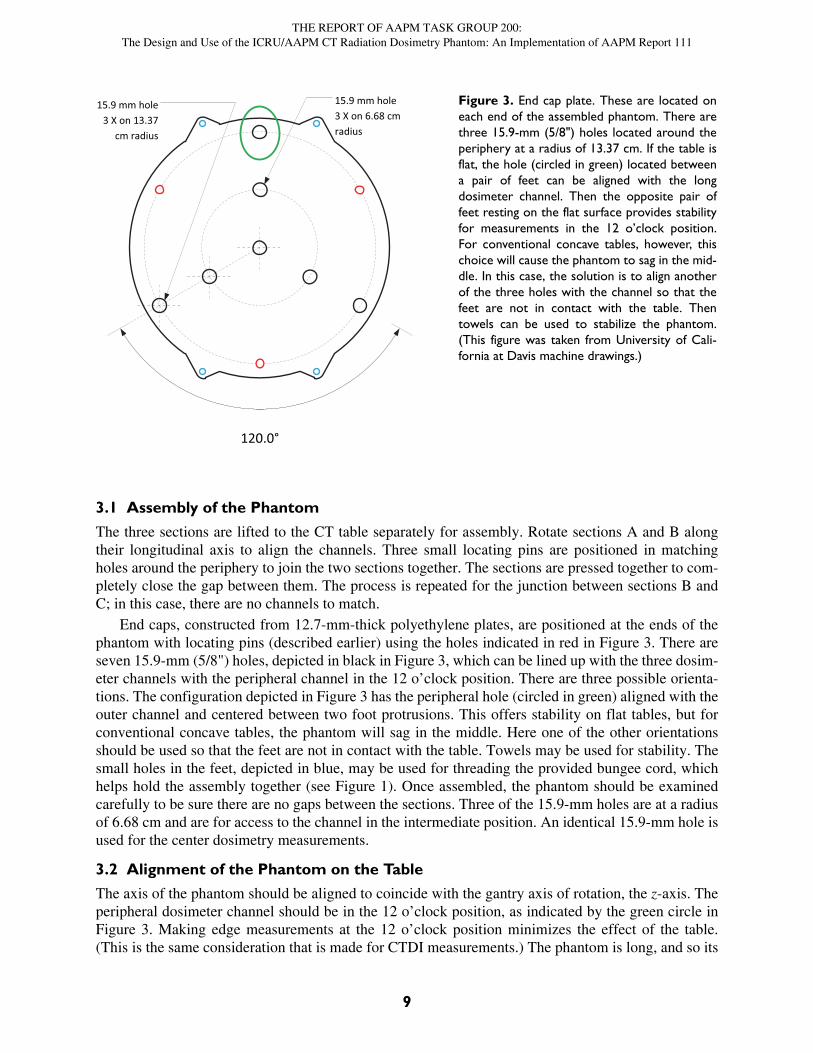
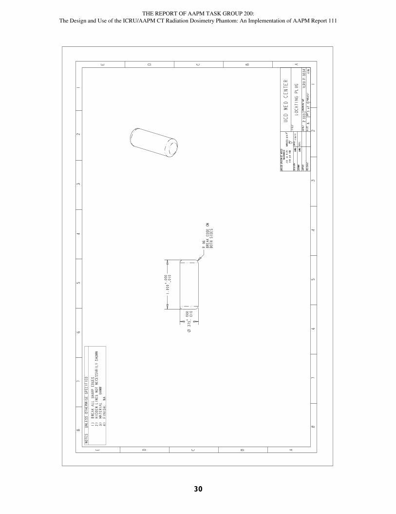
End caps, constructed from 12.7-mm-thick polyethylene plates, are positioned at the ends of thephantom with locating pins (described earlier) using the holes indicated in red in Figure 3. There areseven 15.9-mm (5/8") holes, depicted in black in Figure 3, which can be lined up with the three dosim-eter channels with the peripheral channel in the 12 o’clock position. There are three possible orienta-tions. The configuration depicted in Figure 3 has the peripheral hole (circled in green) aligned with theouter channel and centered between two foot protrusions. This offers stability on flat tables, but forconventional concave tables, the phantom will sag in the middle. Here one of the other orientationsshould be used so that the feet are not in contact with the table. Towels may be used for stability. Thesmall holes in the feet, depicted in blue, may be used for threading the provided bungee cord, whichhelps hold the assembly together (see Figure 1). Once assembled, the phantom should be examinedcarefully to be sure there are no gaps between the sections. Three of the 15.9-mm holes are at a radiusof 6.68 cm and are for access to the channel in the intermediate position. An identical 15.9-mm hole isused for the center dosimetry measurements.

3.2 Alignment of the Phantom on the Table

The axis of the phantom should be aligned to coincide with the gantry axis of rotation, the z-axis. Theperipheral dosimeter channel should be in the 12 o’clock position, as indicated by the green circle inFigure 3. Making edge measurements at the 12 o’clock position minimizes the effect of the table.(This is the same consideration that is made for CTDI measurements.) The phantom is long, and so its

120.0°

15.9 mm hole3 X on 6.68 cm radius

15.9 mm hole3 X on 13.37

cm radius

Figure 3. End cap plate. These are located oneach end of the assembled phantom. There arethree 15.9-mm (5/8") holes located around theperiphery at a radius of 13.37 cm. If the table isflat, the hole (circled in green) located betweena pair of feet can be aligned with the longdosimeter channel. Then the opposite pair offeet resting on the flat surface provides stabilityfor measurements in the 12 o’clock position.For conventional concave tables, however, thischoice will cause the phantom to sag in the mid-dle. In this case, the solution is to align anotherof the three holes with the channel so that thefeet are not in contact with the table. Thentowels can be used to stabilize the phantom.(This figure was taken from University of Cali-fornia at Davis machine drawings.)


10

alignment with system isocenter should be assured by moving the table back and forth within the gan-try, checking the alignment of the phantom from end to end.

4. Measurement Methodology

4.1 Background

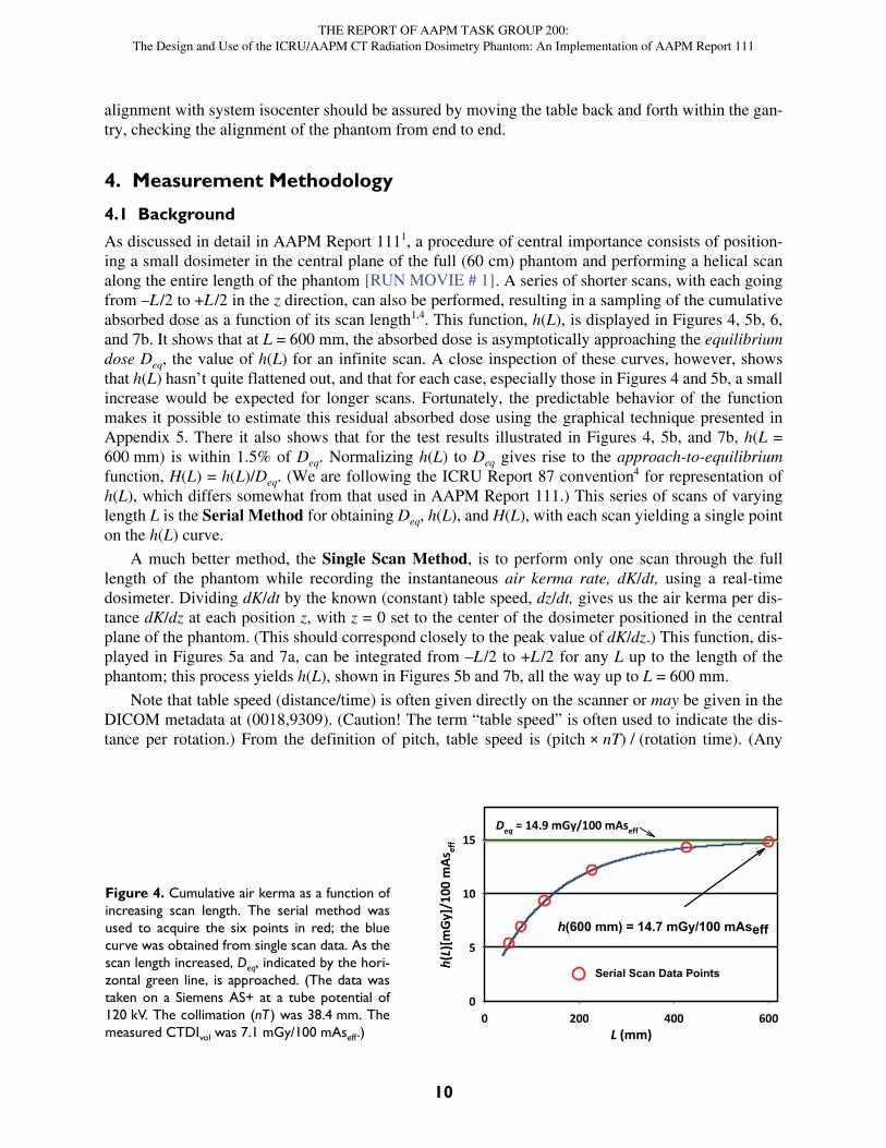
As discussed in detail in AAPM Report 1111, a procedure of central importance consists of position-ing a small dosimeter in the central plane of the full (60 cm) phantom and performing a helical scanalong the entire length of the phantom . A series of shorter scans, with each goingfrom –L/2 to +L /2 in the z direction, can also be performed, resulting in a sampling of the cumulativeabsorbed dose as a function of its scan length1,4. This function, h(L), is displayed in Figures 4, 5b, 6,and 7b. It shows that at L = 600 mm, the absorbed dose is asymptotically approaching the equilibriumdose Deq, the value of h(L) for an infinite scan. A close inspection of these curves, however, showsthat h(L) hasn’t quite flattened out, and that for each case, especially those in Figures 4 and 5b, a smallincrease would be expected for longer scans. Fortunately, the predictable behavior of the functionmakes it possible to estimate this residual absorbed dose using the graphical technique presented inAppendix 5. There it also shows that for the test results illustrated in Figures 4, 5b, and 7b, h(L =600 mm) is within 1.5% of Deq. Normalizing h(L) to Deq gives rise to the approach-to-equilibriumfunction, H(L) = h(L)/Deq. (We are following the ICRU Report 87 convention4 for representation ofh(L), which differs somewhat from that used in AAPM Report 111.) This series of scans of varyinglength L is the Serial Method for obtaining Deq, h(L), and H(L), with each scan yielding a single pointon the h(L) curve.

A much better method, the Single Scan Method, is to perform only one scan through the fulllength of the phantom while recording the instantaneous air kerma rate, dK/dt, using a real-timedosimeter. Dividing dK/dt by the known (constant) table speed, dz/dt, gives us the air kerma per dis-tance dK/dz at each position z, with z = 0 set to the center of the dosimeter positioned in the centralplane of the phantom. (This should correspond closely to the peak value of dK/dz.) This function, dis-played in Figures 5a and 7a, can be integrated from –L/2 to +L /2 for any L up to the length of thephantom; this process yields h(L), shown in Figures 5b and 7b, all the way up to L = 600 mm.

Note that table speed (distance/time) is often given directly on the scanner or may be given in theDICOM metadata at (0018,9309). (Caution! The term “table speed” is often used to indicate the dis-tance per rotation.) From the definition of pitch, table speed is (pitch × nT) / (rotation time). (Any

[RUN MOVIE # 1]

L (mm)0 200 400 600

h(L)

[mGy

]/10

0 m

Asef

f

0

5

10

15Deq = 14.9 mGy/100 mAseff

h(600 mm) = 14.7 mGy/100 mAseff

Serial Scan Data Points

Figure 4. Cumulative air kerma as a function ofincreasing scan length. The serial method wasused to acquire the six points in red; the bluecurve was obtained from single scan data. As thescan length increased, Deq, indicated by the hori-zontal green line, is approached. (The data wastaken on a Siemens AS+ at a tube potential of120 kV. The collimation (nT) was 38.4 mm. Themeasured CTDIvol was 7.1 mGy/100 mAseff.)

https://player.vimeo.com/video/386978404


11

doubts over which parameter is actually being displayed by the machine may be resolved by measur-ing the table speed directly using a tape measure and a stopwatch.)

4.2 Determining Deq and h(L)Both the serial and single scan methods use a small dosimeter embedded in the central plane of thephantom. (The measurements presented in this document were obtained using a small thimble ionchamber, 0.6 cc in volume and 19.7 mm in length (Radcal 10X5-0.6CT). Other dosimeters aredescribed in Appendix 2.) For the serial method, integrating electronics provide the accumulated airkerma for each scan. This approach was used to acquire the six points in red on the h(L) curve in Fig-ure 4. The single scan method requires electronics that can deliver the instantaneous air kerma rate.The single scan method was used to determine the blue curve in Figure 4. The limiting value Deq isapproached as L grows in length with h(600 mm) = 14.7 mGy/100 mAseff. This is well within 1.5% of14.9 mGy/100 mAseff, the value for Deq determined using the method of Appendix 5.

The equivalence of the two techniques is confirmed by the data shown in Figure 4. While theserial method is directly analogous to patient scanning, it is overly burdensome; a separate scan isrequired for every point on the h(L) curve. On the other hand, the single scan method yields the entirecurve with one pass and should, therefore, be used whenever possible.

Though L for the single scan method is simply the distance between the limits of integration, L forthe serial method can be affected by complications, such as overscanning and active collimation.Since these considerations also apply to patient scanning, the definition of L must be general enoughto include both techniques, even though h(L) is to be determined using the single scan method when-ever possible. Thus it is valuable to think in terms of generalizing the concept of directly irradiatedlength. This term was introduced by Dixon and Boone5 to underscore the equivalence between twocommon scanning methods: (1) a conventional scan using a moving table to irradiate a length longerthan a, the width of the beam at the axis of rotation, and (2) a fixed table where the irradiated length isthe beam width a. Application of this concept can be broadened further since only the length that wasdirectly irradiated is important, not the details as to how this was accomplished. (When the scan iscomplete, the important question to ask is, “What was the irradiated length?”)

For helical scans, the International Electrotechnical Commission (IEC) Glossary6 defines thedose-length product, DLP, as CTDIvol × L. In this glossary, L (taken from IEC 60601-2-44, Ed. 3) isdescribed as “the FWHM along a line perpendicular to the tomographic plane at isocenter of the free-in-air dose profile for the entire scan.” This description is consistent with the concept of irradiatedlength, as described in the previous paragraph. Since values for CTDIvol and DLP are provided by theCT scanner, L = DLP/CTDIvol is the value to be used for helical scans. This is how L was determinedfor Figure 4, and there was excellent agreement between the two methods for several other manufac-turers and models using this definition as well7. (Note: the Exposed Range, defined in Part 16 of theDICOM Standard8 for use in CT radiation dose structured reports, is taken from the same IEC reportand so should be equal to the calculated value of L above. Again, this definition is for helical scansonly, and so it is a special case of the general concept of irradiated length.)

4.3 An Example Using Real-Time Data AcquisitionThe following describes the measurement of h(L) using the single scan method (a) at the central axisand (b) at the edge position, which is near the periphery at the point (12 o’clock) farthest from thetable.

Figures 5 and 7 show the data taken from helical scans of the AAPM/ICRU phantom on a PhilipsBrilliance 6 CT machine. The data was acquired using Radcal Accu-Gold electronics with a 10X5-0.6CT ion chamber. Scans were performed at a tube potential of 120 kV, a tube current of 105 mA, arotation time of 0.5 s, a pitch of 0.656, and a collimation, nT, of 4.5 mm (6 × 0.75 mm detector config-


12

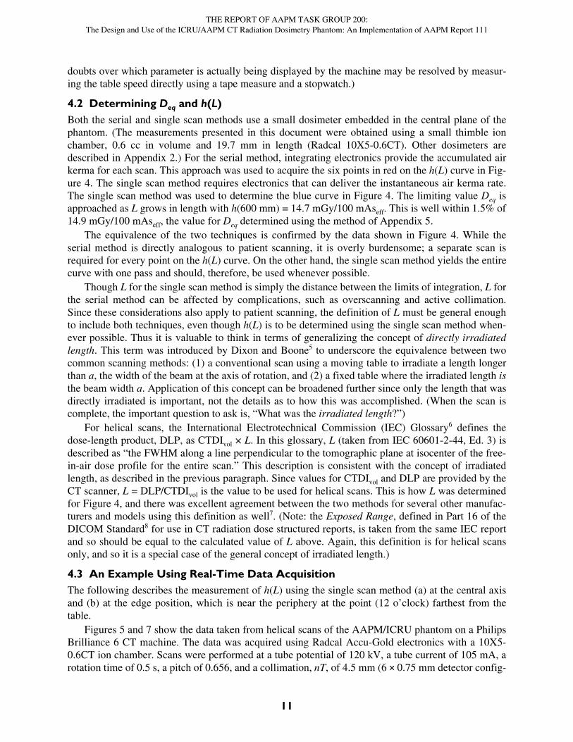
uration). The effective tube current-time product, mAseff, = 0.5 s × 105 mA/0.656 was 80. The tabletravel per rotation b was pitch × collimation = 4.5 mm × 0.656 = 2.95 mm/rotation. The table speed,5.904 mm/s, is b divided by the rotation time. (The scanner reported CTDIvol for these scans, con-firmed by measurement, was 10 mGy/100 mAseff. Note that for the central axis scan for the Philipsscanner in Figure 5, the ratio Deq/CTDIvol is close to that for the Siemens scanner in Figure 4.)

4.3.1 Using Real-Time Dose Measurements along the AxisFigure 5a shows dK/dz as a function of position z, obtained along the central axis of the AAPM/ICRUphantom. (The table speed has been used to convert dK/dt and time, as described in section 3.1.) Fig-ure 5b is a plot of the integral taken over L/2 about the center of the peak of the profile shown in Fig-ure 5a. A limiting value is approached as L is increased beyond 500 mm. (Applying the standardCTDI methodology on this phantom where the table is stationary, the 100-mm pencil chamber wouldcapture only a single point, h(100 mm), on the h(L) curve of Figure 5b. This point is the integral of thedK/dz data between –50 mm and +50 mm in Figure 5a.)

Although at first glance the profile in Figure 5a appears to be noisy, most of the amplitude fluctu-ations are due to the table attenuation occurring during part of every gantry rotation. The contributionto dK/dz due to table attenuation is modulated at a spatial frequency of 1/b. This effect is shown in theinset where a magnified 10-mm portion of the profile is shown. The table travel per rotation b wasshort enough so that the cyclic variation due to table modulation is almost completely smoothed overby the integration process, giving rise to the smooth curve in Figure 5b.

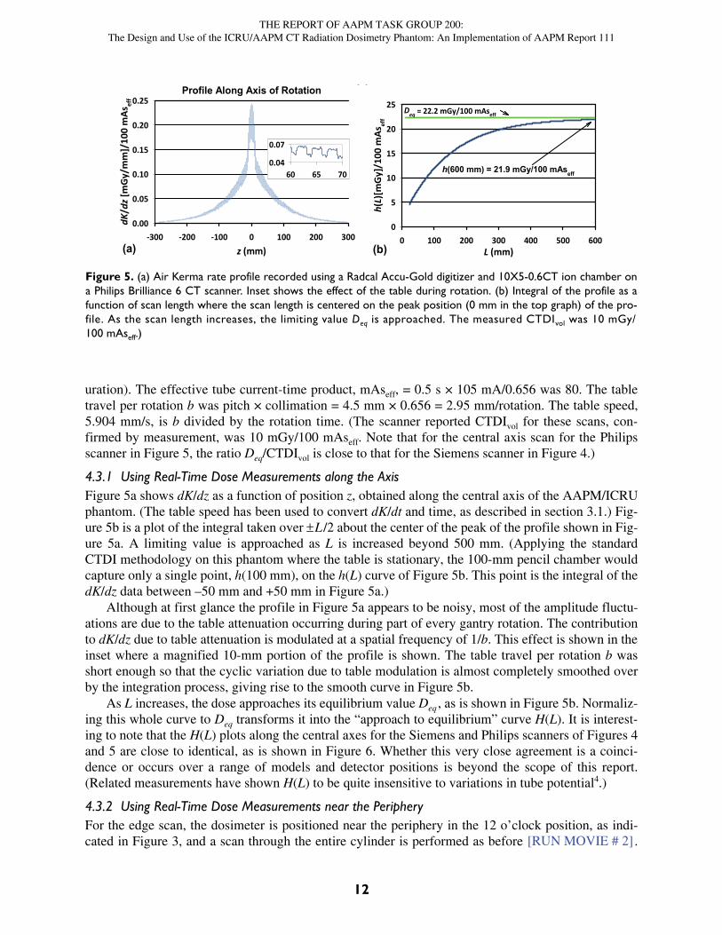
As L increases, the dose approaches its equilibrium value Deq , as is shown in Figure 5b. Normaliz-ing this whole curve to Deq transforms it into the “approach to equilibrium” curve H(L). It is interest-ing to note that the H(L) plots along the central axes for the Siemens and Philips scanners of Figures 4and 5 are close to identical, as is shown in Figure 6. Whether this very close agreement is a coinci-dence or occurs over a range of models and detector positions is beyond the scope of this report.(Related measurements have shown H(L) to be quite insensitive to variations in tube potential4.)

4.3.2 Using Real-Time Dose Measurements near the PeripheryFor the edge scan, the dosimeter is positioned near the periphery in the 12 o’clock position, as indi-cated in Figure 3, and a scan through the entire cylinder is performed as before .

(a) (b)

Profile Along Axis of Rotation

z (mm)-300 -200 -100 0 100 200 300

dK/d

z [m

Gy/

mm

]/10

0 m

Asef

f

0.00

0.05

0.10

0.15

0.20

0.25

60 65 700.04

0.07

L (mm)0 100 200 300 400 500 600

h(L)

[mG

y]/1

00 m

Asef

f

0

5

10

15

20

25 Deq = 22.2 mGy/100 mAseff

h(600 mm) = 21.9 mGy/100 mAseff

Figure 5. (a) Air Kerma rate profile recorded using a Radcal Accu-Gold digitizer and 10X5-0.6CT ion chamber ona Philips Brilliance 6 CT scanner. Inset shows the effect of the table during rotation. (b) Integral of the profile as afunction of scan length where the scan length is centered on the peak position (0 mm in the top graph) of the pro-file. As the scan length increases, the limiting value Deq is approached. The measured CTDIvol was 10 mGy/100 mAseff.)

[RUN MOVIE # 2]



13

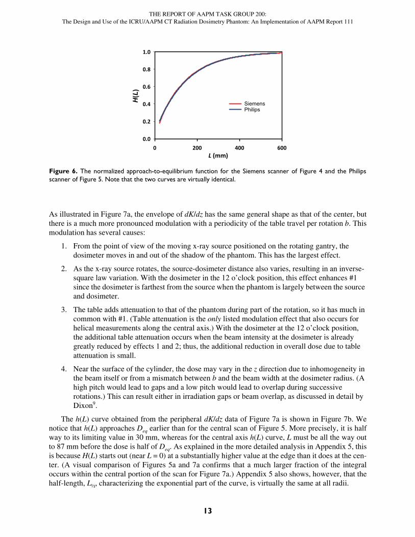
As illustrated in Figure 7a, the envelope of dK/dz has the same general shape as that of the center, butthere is a much more pronounced modulation with a periodicity of the table travel per rotation b. Thismodulation has several causes:

1. From the point of view of the moving x-ray source positioned on the rotating gantry, the dosimeter moves in and out of the shadow of the phantom. This has the largest effect.

2. As the x-ray source rotates, the source-dosimeter distance also varies, resulting in an inverse-square law variation. With the dosimeter in the 12 o’clock position, this effect enhances #1 since the dosimeter is farthest from the source when the phantom is largely between the source and dosimeter.

3. The table adds attenuation to that of the phantom during part of the rotation, so it has much in common with #1. (Table attenuation is the only listed modulation effect that also occurs for helical measurements along the central axis.) With the dosimeter at the 12 o’clock position, the additional table attenuation occurs when the beam intensity at the dosimeter is already greatly reduced by effects 1 and 2; thus, the additional reduction in overall dose due to table attenuation is small.

4. Near the surface of the cylinder, the dose may vary in the z direction due to inhomogeneity in the beam itself or from a mismatch between b and the beam width at the dosimeter radius. (A high pitch would lead to gaps and a low pitch would lead to overlap during successive rotations.) This can result either in irradiation gaps or beam overlap, as discussed in detail by Dixon9.

The h(L) curve obtained from the peripheral dK/dz data of Figure 7a is shown in Figure 7b. Wenotice that h(L) approaches Deq earlier than for the central scan of Figure 5. More precisely, it is halfway to its limiting value in 30 mm, whereas for the central axis h(L) curve, L must be all the way outto 87 mm before the dose is half of Deq. As explained in the more detailed analysis in Appendix 5, thisis because H(L) starts out (near L = 0) at a substantially higher value at the edge than it does at the cen-ter. (A visual comparison of Figures 5a and 7a confirms that a much larger fraction of the integraloccurs within the central portion of the scan for Figure 7a.) Appendix 5 also shows, however, that thehalf-length, L½, characterizing the exponential part of the curve, is virtually the same at all radii.

L (mm)0 200 400 600

H(L

)0.0

0.2

0.4

0.6

0.8

1.0

SiemensPhilips

Figure 6. The normalized approach-to-equilibrium function for the Siemens scanner of Figure 4 and the Philipsscanner of Figure 5. Note that the two curves are virtually identical.


14

4.3.3 Choosing Scanning Parameters for the Peripheral Dose Profile

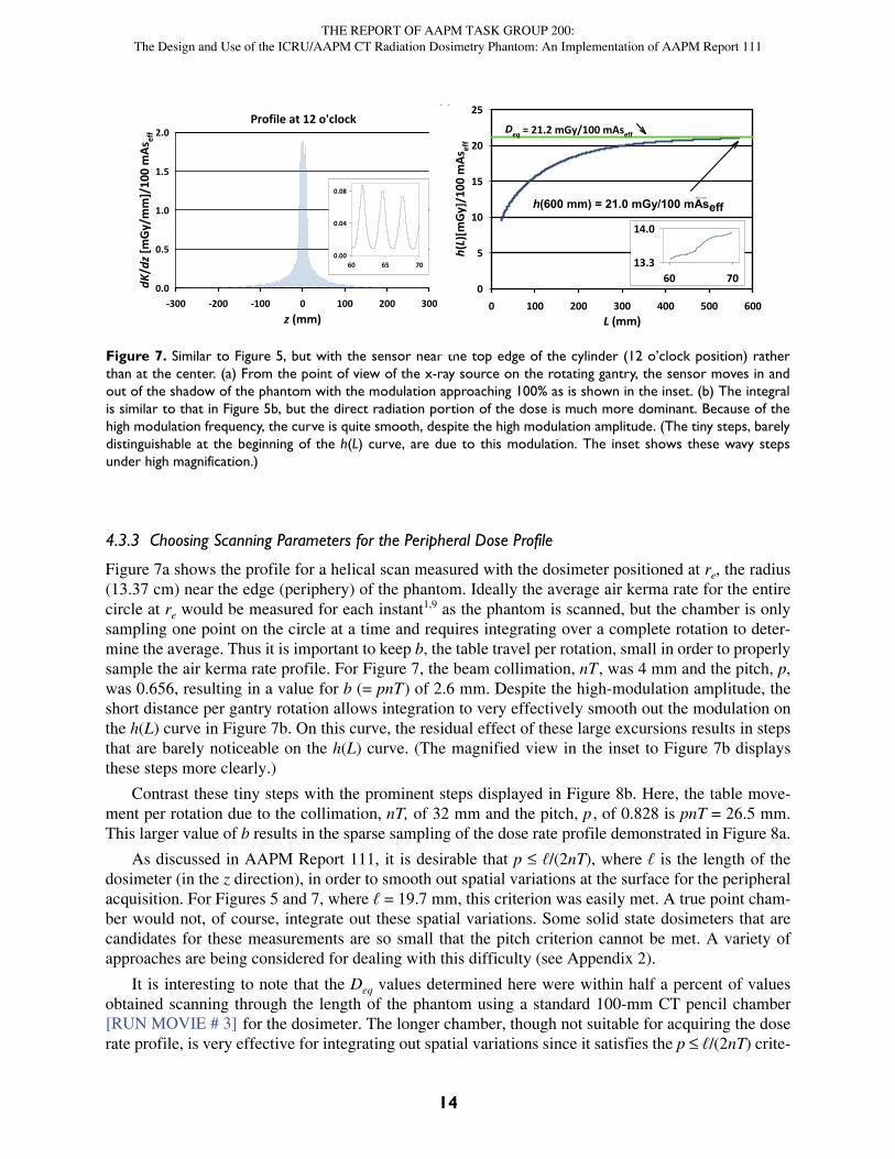
Figure 7a shows the profile for a helical scan measured with the dosimeter positioned at re, the radius(13.37 cm) near the edge (periphery) of the phantom. Ideally the average air kerma rate for the entirecircle at re would be measured for each instant1,9 as the phantom is scanned, but the chamber is onlysampling one point on the circle at a time and requires integrating over a complete rotation to deter-mine the average. Thus it is important to keep b, the table travel per rotation, small in order to properlysample the air kerma rate profile. For Figure 7, the beam collimation, nT , was 4 mm and the pitch, p,was 0.656, resulting in a value for b (= pnT) of 2.6 mm. Despite the high-modulation amplitude, theshort distance per gantry rotation allows integration to very effectively smooth out the modulation onthe h(L) curve in Figure 7b. On this curve, the residual effect of these large excursions results in stepsthat are barely noticeable on the h(L) curve. (The magnified view in the inset to Figure 7b displaysthese steps more clearly.)

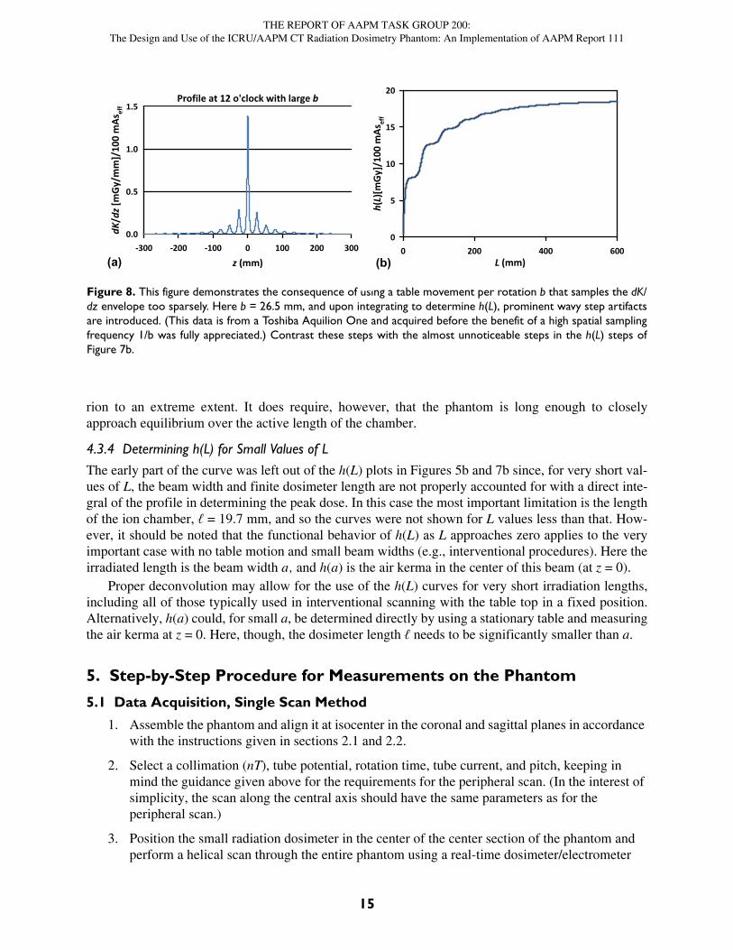
Contrast these tiny steps with the prominent steps displayed in Figure 8b. Here, the table move-ment per rotation due to the collimation, nT, of 32 mm and the pitch, p , of 0.828 is pnT = 26.5 mm.This larger value of b results in the sparse sampling of the dose rate profile demonstrated in Figure 8a.

As discussed in AAPM Report 111, it is desirable that p ℓ/(2nT), where ℓ is the length of thedosimeter (in the z direction), in order to smooth out spatial variations at the surface for the peripheralacquisition. For Figures 5 and 7, where ℓ = 19.7 mm, this criterion was easily met. A true point cham-ber would not, of course, integrate out these spatial variations. Some solid state dosimeters that arecandidates for these measurements are so small that the pitch criterion cannot be met. A variety ofapproaches are being considered for dealing with this difficulty (see Appendix 2).

It is interesting to note that the Deq values determined here were within half a percent of valuesobtained scanning through the length of the phantom using a standard 100-mm CT pencil chamber

for the dosimeter. The longer chamber, though not suitable for acquiring the doserate profile, is very effective for integrating out spatial variations since it satisfies the p ℓ/(2nT) crite-

(a) (b)

Profile at 12 o'clock

z (mm)-300 -200 -100 0 100 200 300

dK/d

z [m

Gy/m

m]/

100

mAs

eff

0.0

0.5

1.0

1.5

2.0

L (mm)0 100 200 300 400 500 600

h(L)

[mGy

]/10

0 m

Asef

f

0

5

10

15

20

25

Deq = 21.2 mGy/100 mAseff

h(600 mm) = 21.0 mGy/100 mAseffh(L) inset

60 7013.3

14.0

60 65 700.00

0.04

0.08

Figure 7. Similar to Figure 5, but with the sensor near the top edge of the cylinder (12 o’clock position) ratherthan at the center. (a) From the point of view of the x-ray source on the rotating gantry, the sensor moves in andout of the shadow of the phantom with the modulation approaching 100% as is shown in the inset. (b) The integralis similar to that in Figure 5b, but the direct radiation portion of the dose is much more dominant. Because of thehigh modulation frequency, the curve is quite smooth, despite the high modulation amplitude. (The tiny steps, barelydistinguishable at the beginning of the h(L) curve, are due to this modulation. The inset shows these wavy stepsunder high magnification.)

[RUN MOVIE # 3]



15

rion to an extreme extent. It does require, however, that the phantom is long enough to closelyapproach equilibrium over the active length of the chamber.

4.3.4 Determining h(L) for Small Values of L

The early part of the curve was left out of the h(L) plots in Figures 5b and 7b since, for very short val-ues of L, the beam width and finite dosimeter length are not properly accounted for with a direct inte-gral of the profile in determining the peak dose. In this case the most important limitation is the lengthof the ion chamber, ℓ = 19.7 mm, and so the curves were not shown for L values less than that. How-ever, it should be noted that the functional behavior of h(L) as L approaches zero applies to the veryimportant case with no table motion and small beam widths (e.g., interventional procedures). Here theirradiated length is the beam width a, and h(a) is the air kerma in the center of this beam (at z = 0).

Proper deconvolution may allow for the use of the h(L) curves for very short irradiation lengths,including all of those typically used in interventional scanning with the table top in a fixed position.Alternatively, h(a) could, for small a, be determined directly by using a stationary table and measuringthe air kerma at z = 0. Here, though, the dosimeter length ℓ needs to be significantly smaller than a.

5. Step-by-Step Procedure for Measurements on the Phantom

5.1 Data Acquisition, Single Scan Method

1. Assemble the phantom and align it at isocenter in the coronal and sagittal planes in accordance with the instructions given in sections 2.1 and 2.2.

2. Select a collimation (nT), tube potential, rotation time, tube current, and pitch, keeping in mind the guidance given above for the requirements for the peripheral scan. (In the interest of simplicity, the scan along the central axis should have the same parameters as for the peripheral scan.)

3. Position the small radiation dosimeter in the center of the center section of the phantom and perform a helical scan through the entire phantom using a real-time dosimeter/electrometer

Figure 8. This figure demonstrates the consequence of using a table movement per rotation b that samples the dK/dz envelope too sparsely. Here b = 26.5 mm, and upon integrating to determine h(L), prominent wavy step artifactsare introduced. (This data is from a Toshiba Aquilion One and acquired before the benefit of a high spatial samplingfrequency 1/b was fully appreciated.) Contrast these steps with the almost unnoticeable steps in the h(L) steps ofFigure 7b.

(a) (b)

Profile at 12 o'clock with large b

z (mm)-300 -200 -100 0 100 200 300

dK/d

z [m

Gy/m

m]/

100

mAs

eff

0.0

0.5

1.0

1.5

L (mm)0 200 400 600

h(L)

[mGy

]/10

0 m

Asef

f

0

5

10

15

20


16

combination. The real-time data and table speed can be used to determine dK/dz, as described earlier.

4. Repeat for all tube potentials and bowtie/flat filter combinations of interest.

5. Position the small dosimeter in the central plane of the phantom at radius re in the 12 o’clock position. Perform a helical scan through the entire phantom using a real-time dosimeter/electrometer combination. Again, the real-time data and table speed can be used to determine dK/dz, as described earlier.

6. Repeat for the tube potentials and bowtie/flat filter combinations used in step 4.

5.2 Data Acquisition, Serial Method

With the setup the same as above, the serial scan method could be used as an alternative. The inte-grated dose for each scan as a function of increasing scan length is the function h(L) where L = DLP/CTDIvol, as described in section 3.1. As previously stated, the single scan method should be usedwherever possible.

5.3 Additional Collimations and Pitch Values

As discussed in detail in AAPM Report 111 and the references cited therein, (particularly Dixon,Munley and Bayram10 and Dixon and Ballard19) the results for all collimations and all pitch values arereadily determined from the particular values chosen for the measurements at one specific collimationand pitch. Note that these results are robust, even in the presence of the heel effect. Thus, the collima-tion and pitch utilized for measurement should be chosen to meet the requirements discussed above(i.e., a small value for b) to ensure accuracy.

5.4 Data Analysis

1. For the long helical scans, dK/dz can be determined from the recording of dK/dt and the table speed, as described above.

2. If the real-time chamber is used, the integrated value may also be displayed directly for a useful check of the numerical integration. This should be recorded along with the dose rate data.

3. The zero of the distance scale is set to mid-peak of the dose profile, which occurs when the dosimeter is passing through the center of the beam. A further refinement is to view the dose profile data using a log scale for the ordinate and using that to determine the approximate center of symmetry.

4. The dose rate profile dK/dz(z) is integrated from –L/2 to +L/2. The result is plotted as a function of L, where L is varied from zero to a value such that the integral no longer increases with integration length. The resultant function is h(L), and its limiting value is, of course, Deq. When h(L) is divided by Deq, the approach to equilibrium function H(L), which varies from zero to 1, is obtained.

5. For the serial method described in 4.2, specific points of the h(L) curve are obtained directly. To get H(L), divide by Deq, the value for a scan encompassing the entire phantom.

Both the central and edge functions hc(L) and he(L), respectively, are to be retained. Equivalently,we can retain Hc(L) and He(L) along with their limiting values, Deq,c and Deq,e, respectively. The H(L)


17

values alone are not enough since the central and edge values have different limits. For example, if weestimate the spatial average value of H(L) with the familiar 1/3 and 2/3 coefficients from CTDIvol,

The important parameter from AAPM Report 111 can be expressed as

Then

where is an estimate of the spatial average of H over the entire cross section at position L.

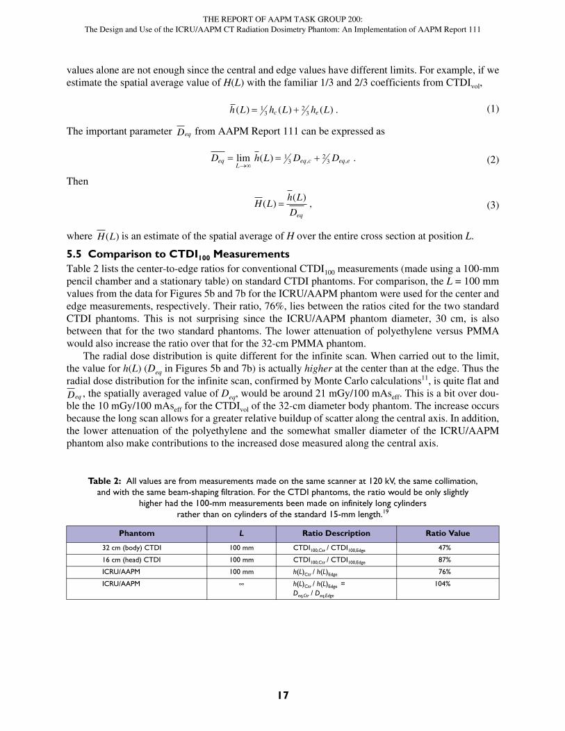
5.5 Comparison to CTDI100 MeasurementsTable 2 lists the center-to-edge ratios for conventional CTDI100 measurements (made using a 100-mmpencil chamber and a stationary table) on standard CTDI phantoms. For comparison, the L = 100 mmvalues from the data for Figures 5b and 7b for the ICRU/AAPM phantom were used for the center andedge measurements, respectively. Their ratio, 76%, lies between the ratios cited for the two standardCTDI phantoms. This is not surprising since the ICRU/AAPM phantom diameter, 30 cm, is alsobetween that for the two standard phantoms. The lower attenuation of polyethylene versus PMMAwould also increase the ratio over that for the 32-cm PMMA phantom.

The radial dose distribution is quite different for the infinite scan. When carried out to the limit,the value for h(L) (Deq in Figures 5b and 7b) is actually higher at the center than at the edge. Thus theradial dose distribution for the infinite scan, confirmed by Monte Carlo calculations11, is quite flat and

, the spatially averaged value of Deq, would be around 21 mGy/100 mAseff. This is a bit over dou-ble the 10 mGy/100 mAseff for the CTDIvol of the 32-cm diameter body phantom. The increase occursbecause the long scan allows for a greater relative buildup of scatter along the central axis. In addition,the lower attenuation of the polyethylene and the somewhat smaller diameter of the ICRU/AAPMphantom also make contributions to the increased dose measured along the central axis.

Table 2: All values are from measurements made on the same scanner at 120 kV, the same collimation,and with the same beam-shaping filtration. For the CTDI phantoms, the ratio would be only slightly

higher had the 100-mm measurements been made on infinitely long cylindersrather than on cylinders of the standard 15-mm length.19

Phantom L Ratio Description Ratio Value

32 cm (body) CTDI 100 mm CTDI100,Ctr / CTDI100,Edge 47%

16 cm (head) CTDI 100 mm CTDI100,Ctr / CTDI100,Edge 87%

ICRU/AAPM 100 mm h(L)Ctr / h(L)Edge 76%

ICRU/AAPM h(L)Ctr / h(L)Edge = Deq,Ctr / Deq,Edge

104%

(1)h L h L h Lc e( ) ( ) ( ) . 13

23

Deq

(2)D h L D DeqL

eq c eq e

lim ( ) ., ,1

32

3

(3)H Lh L

Deq

( )( )

,

H L( )

Deq


18

6. Practical Implementation of the Measurement Methodology

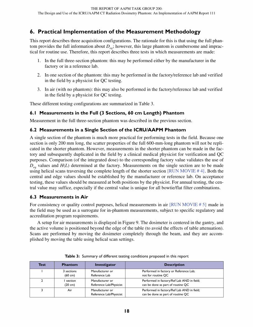
This report describes three acquisition configurations. The rationale for this is that using the full phan-tom provides the full information about Deq; however, this large phantom is cumbersome and imprac-tical for routine use. Therefore, this report describes three tests in which measurements are made:

1. In the full three-section phantom: this may be performed either by the manufacturer in the factory or in a reference lab.

2. In one section of the phantom: this may be performed in the factory/reference lab and verified in the field by a physicist for QC testing.

3. In air (with no phantom): this may also be performed in the factory/reference lab and verified in the field by a physicist for QC testing.

These different testing configurations are summarized in Table 3.

6.1 Measurements in the Full (3 Sections, 60 cm Length) Phantom

Measurement in the full three-section phantom was described in the previous section.

6.2 Measurements in a Single Section of the ICRU/AAPM Phantom

A single section of the phantom is much more practical for performing tests in the field. Because onesection is only 200 mm long, the scatter properties of the full 600-mm-long phantom will not be repli-cated in the shorter phantom. However, measurements in the shorter phantom can be made in the fac-tory and subsequently duplicated in the field by a clinical medical physicist for verification and QCpurposes. Comparison (of the integrated dose) to the corresponding factory value validates the use ofDeq values and H(L) determined at the factory. Measurements on the single section are to be madeusing helical scans traversing the complete length of the shorter section . Both thecentral and edge values should be established by the manufacturer or reference lab. On acceptancetesting, these values should be measured at both positions by the physicist. For annual testing, the cen-tral value may suffice, especially if the central value is unique for all bowtie/flat filter combinations.

6.3 Measurements in Air

For consistency or quality control purposes, helical measurements in air made inthe field may be used as a surrogate for in-phantom measurements, subject to specific regulatory andaccreditation program requirements.

A setup for air measurements is displayed in Figure 9. The dosimeter is centered in the gantry, andthe active volume is positioned beyond the edge of the table (to avoid the effects of table attenuation).Scans are performed by moving the dosimeter completely through the beam, and they are accom-plished by moving the table using helical scan settings.

Table 3: Summary of different testing conditions proposed in this report

Test Phantom Investigator Description

1 3 sections(60 cm)

Manufacturer or Reference Lab

Performed in factory or Reference Lab; not for routine QC

2 1 section(20 cm)

Manufacturer or Reference Lab/Physicist

Performed in factory/Ref Lab AND in field; can be done as part of routine QC

3 Air Manufacturer or Reference Lab/Physicist

Performed in factory/Ref Lab AND in field; can be done as part of routine QC

[RUN MOVIE # 4]

[RUN MOVIE # 5]




19

It should be noted that for in-air measurements, one scan per condition (tube potential, bowtie/fil-ter combination—See #4 of Section 4.1) is performed with the dosimeter at isocenter.

In addition to serving as a replacement for actual phantom measurements, in-air measurementscan serve other purposes, so it is important that they are made carefully. They can be used to establishtube current linearity—thus allowing a phantom measurement to be made at a tube current and rota-tion time chosen for convenience—and signal-to-noise considerations. They also can be used to con-firm the linear scaling of integrated dose with changes in z-axis collimation aperture a1, greatlyreducing the required number of phantom measurements. (Indeed, this may be the best place to mea-sure or verify the values of a. The vendor’s relative values of a can be deduced from the CTDIvol orefficiency values displayed on the machine. The air scans present a simple and straightforwardmethod for the verification of the indicated values.)

The integrated value (directly displayed by either the integrating electrometer or the real-timeelectrometer) is all that is necessary for properly scaling tube current-time product and collimation. Arecording of the dose profile in air may be used to verify beam uniformity and with care might be ofsome value in determining beam width a. However, the finite length of the small chamber needs to beaccounted for if used for this purpose. Chamber length is not relevant for determining tube current-time product, effective tube current-time product, or collimation dependence since, as the chamberpasses through the beam, every point in the beam is sampled by the entire chamber. Verifying tubecurrent-time product or effective tube current-time product linearity is conveniently done in air(though we recognize that the manufacturers may have established more direct and precise means fordoing this).

It is understood that the in-air measurements, as described, sample the beam only along the axis ofrotation. In principle, it is possible that two bowtie designs would have the same central beam proper-ties and yet be quite different when the entire beam is explored. We do not expect this coincidental

Figure 9. A figure from the TG-111 report. Thimble ionization chamber free-in-air and aligned along the axis ofrotation. The chamber is attached to an extender rod from a lab stand, and the assembly is illuminated by the CTsystem alignment laser lights.


20

behavior to be of much consequence for annual physics testing. However, in order to eliminate thispossibility in acceptance testing, the single-section test described for acceptance testing in section 5.2should be performed along with the air measurement. As in section 5.2, if the air measurement isunique for each bowtie/flat filter combination, the air measurement should suffice for annual physicstesting. If there is an ambiguity, an off-axis air measurement12 could be used to resolve any equivocal-ity.

6.4 Measurements in Very Wide Beams and Using Stationary Tables

An example CT system with a very wide (e.g., 16 cm) beam width is the Toshiba Aquilion ONE. Inthe helical scan mode this machine may be tested as described in the procedure above for beam widthsup to 8 cm. The full detector width of 16 cm is used only with a stationary table in the volume acquisi-tion mode. Although Dixon and Boone5 have rigorously demonstrated self-consistency between thetwo types of scans, an alternative—the pseudohelical scan method described by Lin and Herrns-dorf13—has been specifically developed for acquiring dK/dz using a stationary table with the tube onand with the gantry continuously rotating continuously rotating . This is a specialcase of the single scan method. Here the dosimeter is mounted on an assembly that is pushed or pulledat constant speed through the phantom. In this case, the dosimeter channels must pass completelythrough the phantom, end to end. One way to accomplish this is to assemble the phantom from threesections of type A. For the edge position at 12 o’clock, high spatial frequency modulation is bestachieved by moving the dosimeter slowly through the phantom along with the utilization of a highgantry rotation frequency. (This may be thought of as using a low pseudopitch.) This results in high-frequency sampling of the dose profile envelope. The limiting dose Deq and approach to equilibriumfunction H(L) are determined in precisely the same way as they are for the helical scans describedabove.

There is also a form of the serial method that can be implemented for this special case. This isdescribed in AAPM Report 111 where the notion of irradiated length is utilized when a scan is madewith a stationary table and a wide beam. Here the dosimeter is positioned in the central plane of thephantom, as before, and the phantom is centered in the beam. The integrated dose per rotation is deter-mined. The length L is simply the width of the beam. The point h(L) is thus determined for each valueof L used. L may be defined, for example, as the FWHM of the beam along the central axis, or it maybe deduced by comparison of measurements using a long helical scan. Without moving the phantom,this limits us to values of L up to that of the widest beam available, aw. This limitation presents prob-lems in establishing Deq. One way to obtain h(L) for values of L that go beyond aw and capture more ofthe scatter tail is to do the following:

1. First be sure that h(aw) has been determined.

2. Choose a beam width a* for the scanner (where a* aw).

3. Translate the phantom (in the z direction) so that the dosimeter is positioned at z = aw/2 + a*. (The dosimeter remains in the central plane of the phantom; the phantom is no longer centered in the beam.)

4. Perform a fixed-table scan (with the same techniques used to acquire h(L) for values of L < aw) and record the reading on the dosimeter.

5. Move the phantom and dosimeter to the opposite side of the scanning plane, i.e., to z = –(aw/2 + a*).

6. Repeat step 3.

[RUN MOVIE # 6]



21

7. Add the two readings from steps 3 and 5 to the value recorded for L = aw. This will be h(aw + 2a*).

When establishing position, it will be important to match the half-maximum end points of aw and a*.This method can be used to extend L up to 3aw and then extended again to go from L = 3aw to L = 5aw,7aw, etc. Clearly, if possible to implement, a single-scan method is much preferred.

7. ConclusionsBy extending the scan length to that required for approaching the limiting value, Deq, the ICRU/AAPM phantom and measurement techniques described here address, in a simple and natural way, thelimitations of the CTDI methodology presented in the introduction. These include the systematicexclusion of dose accumulating for scans longer than 100 mm, exclusion of primary beam for scan-ners with beam widths in excess of 100 mm, and potential unsuitability for stationary table applica-tions. Together, Deq and the remarkably robust “approach to equilibrium function” H(L) promise topresent a simple and intuitive picture describing the radiation output of the machine by describing it interms of the dose to a standard (infinite) phantom. Further, a high correlation between Deq and CTDImeasurements has been demonstrated4,14. This is not altogether surprising, since both are indicators ofmachine output. This correlation will facilitate the adoption of the ICRU/AAPM phantom as a futurestandard.

8. References1 American Association of Physicists in Medicine. “Comprehensive methodology for the evalua-

tion of radiation dose in x-ray computed tomography.” Report of AAPM Task Group 111: The Future of CT Dosimetry. College Park, MD: AAPM, 2010.

2 Boone, J. M. (2007). “The trouble with CTDI100.” Med. Phys. 34(4):1364–71.3 Attix, F. H. Introduction to Radiological Physics and Radiation Dosimetry. New York: John

Wiley & Sons, Inc., 1986.4 Boone, J. M., et al. (2012). “CT Dosimetry in Phantoms.” In ICRU Report 87, Radiation Dose

and Image-Quality Assessment in Computed Tomography. JICRU 12(1):67–87.5 Dixon, R. L. and J. M. Boone. (2010). “Cone beam CT dosimetry: A unified and self-consistent

approach including all scan modalities—With or without phantom motion.” Med. Phys. 37(6):2703–18.

6 International Electrotechnical Commission. Glossary. Available at std.iec.ch/glossary. Search for “doselength product” and select “English.”

7 Data and analysis by Sarah McKenney.8 DICOM Standard of NEMA PS3 / ISO 12052. Part 16. Digital Imaging and Communications in

Medicine (DICOM) Standard. Rosslyn, VA: National Electrical Manufacturers Association. Available free at https://www.dicomstandard.org/.

9 Dixon, R. L. (2003). “A new look at CT dose measurement: Beyond CTDI.” Med. Phys. 30(6):1272–80.

10 Dixon, R. L., M. T. Munley, and E. Bayram. (2005). “An improved analytical model for CT dose simulation with a new look at the theory of CT dose.” Med. Phys. 32(12):3712–28.

11 Bakalyar, D. M., W. Feng, and S. McKenney. (2014). “Diameter Dependency of the Radial Dose Distribution in a Long Polyethylene Cylinder.” Med. Phys. 41:405.

12 Boone, J. M. (2009). “Method for evaluating bow tie filter angle-dependent attenuation in CT: Theory and simulation results.” Med. Phys. 37(3):40–48.

https://www.dicomstandard.org/


22

13 Lin, P. J. and L. Herrnsdorf. (2010). “Pseudohelical Scan for the Dose Profile Measurements of 160-mm-Wide Cone-Beam MDCT.” AJR194:897–902.

14 McKenney, SE. “Computed Tomography Dose and Image Quality Characterization Using Real-Time Dosimeter Measurements.” (Doctoral dissertation). Retrieved from ProQuest Dissertations Publishing (Accession No. 3614244); 2013.

15 American Association of Physicists in Medicine. “Use of Water Equivalent Diameter for Calcu-lating Patient Size and Size-Specific Dose Estimates (SSDE) in CT.” Report of AAPM Task Group 220: Determination of a Patient Size Metric for CT Size Specific Dose Estimation. Col-lege Park, MD: AAPM, 2014.

16 American Association of Physicists in Medicine. “Size Specific Dose Estimates (SSDE) in Pedi-atric and Adult CT Examinations.” Report of AAPM Task Group 204. College Park, MD: AAPM, 2011.

17 Ford, E. S., L. M. Maynard, and C. Li. (2014). “Trends in Mean Waist Circumference and Abdominal Obesity Among US Adults, 1999–2012.” JAMA 312(11):1151–53.

18 Bakalyar, D. M. (2016). “In Search of Infinity: Finding the Limiting Dose for An Infinite CT Scan On a Cylinder of Finite Length.” Med. Phys. 43(6):3395.

19 Dixon, R. L. and A. C. Ballard. (2007). “Experimental validation of a versatile system of CT dosimetry using a conventional ion chamber: Beyond CTDI100.” Med. Phys. 34(8):3399–413.


23

Appendix 1:

Measurements in Other GeometriesEven though related systems (e.g., C-arm cone-beam CT) have much in common with MDCT, specialchallenges place the application of our methodology to these systems well beyond the scope of thisreport. These problems include, but are not limited to, sub-360° acquisition and the inability for theoperator to directly control the tube potential. Also, in many cases, the extent of the beam in the xyplane is such that it does not intercept the entire patient. For example, it is often only 25 cm, whereasin diagnostic CT machines, the beam can usually span 50 cm for body scans. So, for the ICRU/AAPMphantom as well as the 32-cm CTDI body phantom an outer circular region of the phantom is not irra-diated in the same way as the inner part . This is acceptable for imaging if only theinner part is of interest. However, the radial behavior of the dose profile will differ from that of aphantom completely enveloped by a broad beam, and further study may be necessary to properly esti-mate in these systems. (A smaller-diameter phantom is a partial solution but leaves unaddressedthe problem of dose delivery when the breadth of a body is not contained within a beam—an occa-sional problem in MDCT but common in these other systems.)

[RUN MOVIE # 7]

Deq



24

Appendix 2:

Measurement Equipment NoteThe serial method has been successfully applied using small ion chambers (Model 2571 Farmer cham-ber) by several members of TG-200. Small solid-state dosimeters with their potentially high spatialresolution and sensitivity, coupled with appropriate recording electronics, present another possibilityfor the single-scan method. It should be noted that such devices may present some unique challenges.The first is that the device may be sensitive to energy dependencies (e.g., beam hardening). For mea-surements performed at the edge position, the change in energy spectrum caused by the phantom canvary significantly during gantry rotation. Therefore, if this device is to be used in the single-scanmethod, care should be taken and the manufacturer consulted to ensure the proper corrections areused.

Ironically, the high spatial resolution that can be a desirable feature of these small dosimeters maymean that the pitch criterion noted at the end of section 4.3 is not met. One possible solution for thisproblem is to average several scans together with the dosimeter position shifted slightly (in the z direc-tion) relative to the phantom for each scan. Here it is necessary to take care that the dosimeter posi-tions (or, equivalently, dK/dz envelope positions) are matched for the different scans prior toaveraging.


25

Appendix 3:

Supplemental Material AvailableData RecordingA sample Excel workbook, ICRU-AAPM_phantom.xlsx, is provided. This may be modified as expe-rience, need, or convenience dictates. Note that for each kV, only one set of data measurements usingthe phantom is required. Additional rows in the spreadsheet are for air measurements at different col-limation settings or at settings designed to check the linearity of tube current, rotation time, or effec-tive tube current-time product. Separate blank sheets are provided for determining H(L) for each tubepotential. A sample dose profile and integral is included with notes.

AnimationsReferences to seven animations are found in this report. Look for the words in brack-ets. By clicking on this text, a hyperlink will take you to the AAPM website where the animations arestored and can be played.

Tutorial and Example for Fine-Tuning the Determination of Deq.An Excel workbook and a brief document are included for augmenting the discussion in Appendix 5.

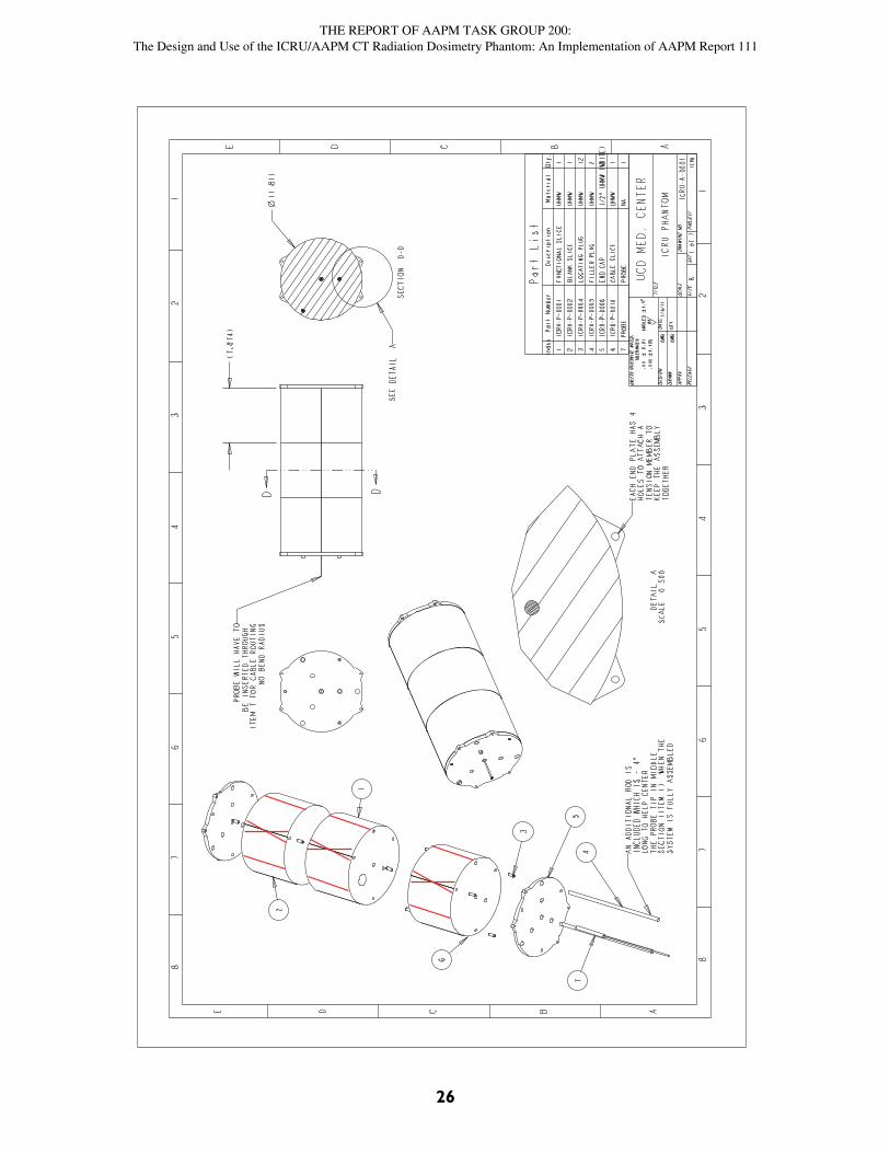
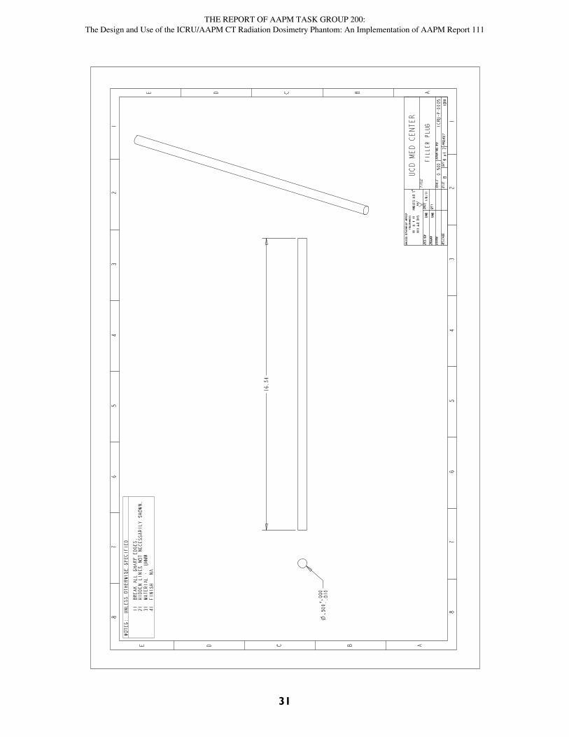
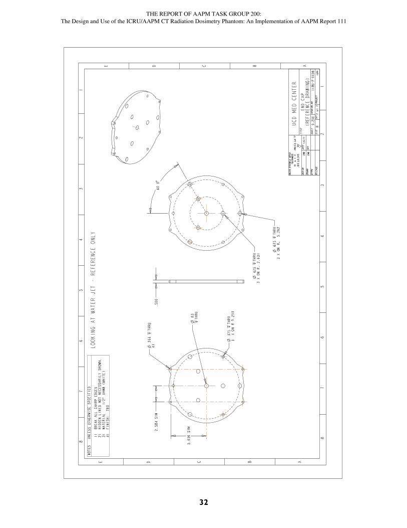
Machine Drawings for PhantomSee the next four pages for phantom construction drawings.

[RUN MOVIE]


26


27

withcentrallineatthe

positionoftheouter

detectorthruhole


28


29


30


31


32


33

Appendix 4:

Corresponding Human Size using Water-Equivalent Diameter

It is instructive to look at the water-equivalent diameter dw discussed at length in AAPM Report No.22015. This is the diameter of a water cylinder having the same mean absorbed dose as the section ofthe patient or phantom under consideration. AAPM Report No. 220 expands the concept of size-spe-cific dose estimate (SSDE) described in AAPM Report No. 20416 to include, in addition to geometry,the effects of the composition and density of the imaged tissue. Utilizing Equation 4 from AAPMReport No. 220,

where is the area-average CT number for the cross-sectional area A of the subject (patient or phan-tom) under consideration. (The definition of d in terms of A is implicit in Equation 4.) With waterequivalence as a metric, we equate the water-equivalent diameter of our phantom to the diameter cor-responding to the waist of human subjects. Thus,

where dH and dP are the human and phantom diameters and H and P are the corresponding CT num-bers. For all phantoms under consideration and in the region of the waist, | | is ≪ 1000, which allowsus to expand the radicals in Equation 5 to lowest order in /1000. Rearranging terms,

How do our phantoms correspond to waist size? A recent study17 puts the current average (men andwomen combined) waist size at 98.5 cm (38.7 inches) with the measurements being made just abovethe iliac crest. (Note that the point of this publication is that the average waist size has increased sig-nificantly over the last decade and that 98.5 cm is an average, not an ideal.) The area average CTnumber (H in Equations 5 and 6) is around zero at the waist. For the 30-cm-diameter ICRU/AAPMphantom, P was –74 for the scans used for Figures 5 and 7. Substituting into Equation 6, this corre-sponds to a human waist size of

(36 inches). The 32-cm CTDI phantom corresponds to a larger person, more likely one with signifi-cant body fat. Set H to –40 to account for the additional adipose tissue in many of these larger people.The CT number for PMMA is around 124. Again substituting into Equation 6, the 32-cm CTDI phan-tom corresponds to a human waist size of

(4)dA A

dww

2 2 1

10001

1000

,

(5)d dHH

PP1

10001

1000

,

(6)d dH PP H

1

2000

.

(7)CH TG, . . .200 30 174 0

200094 2 0 96 90 8

cm cm cm

(8)CH CTDI,( )

.

32 1

124 40

2000101 1 08 109cm cm cm


34

(43 inches). Using this metric, the ICRU/AAPM phantom represents a moderate waist size for westernpopulations, whereas the CTDI phantom better characterizes individuals somewhat larger than aver-age. Both are well within the normal range of adult waist sizes in western populations.


35

Appendix 5:

Fine Tuning DeqFigures 4, 5b, 6, and 7b show that h(L) is closing in on its limiting value Deq when the entire 600 mmof the phantom is scanned. However, it is clear that even at this length (see Section 4.1) h(L) is stillincreasing, i.e., a slightly higher dose would result from a scan through a longer phantom. In what fol-lows, we describe a method for including this residual dose, giving us a more accurate assessment ofDeq.

In its simplest form, the h(L) curve is known to be that of an exponential rise (like that of acharging capacitor) to a limiting value which, in our case, is Deq. That is,

where L½ is the value of L for which the exponential in Equation 9 is equal to ½. Deq(1–) is the valuefor h when L = 0.

is the finite scanning length for which AAPM Report 111 suggests that the cumulative dose is closeenough to Deq for practical purposes. The two forms of Equation 9 are equivalent, but the second formis more convenient for what follows. Rearranging,

Next define the function g(L, D*) using the following relationship:

Take the logarithm (base 2) of Equation 11. Then, using the definition in Equation 12,

which is a straight line (with L as the abscissa and g as the ordinate) as long as h(L) follows the formof an exponential rise to a limit. Because base 2 was used in taking the logarithm, each increase in Lby the half-length L½ results in a decrease in g by 1. (This decrease by 1 corresponds to a reduction ofthe distance between h(L) and its asymptotic limit Deq by half.)

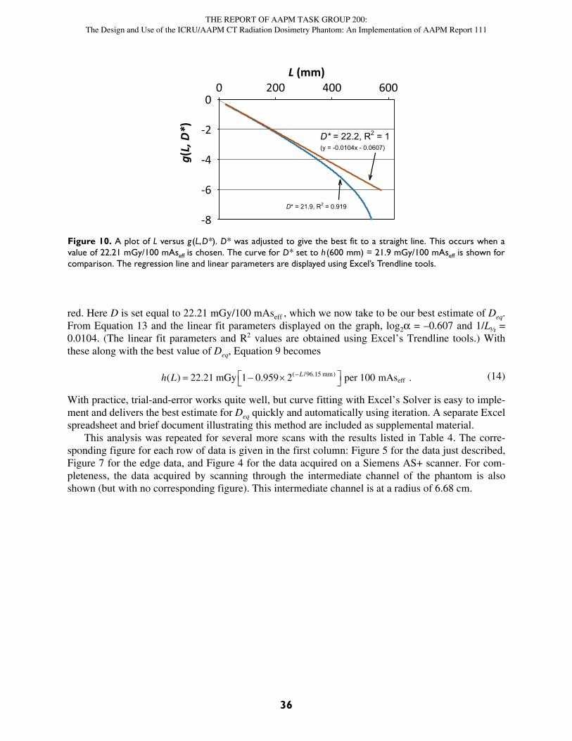
On the other hand, if D* does not equal Deq, a plot of g(L, D*) versus L will deviate from a straightline. This gives us a means of determining the best estimate of Deq from h(L). As an example, considerFigure 10, which uses the experimentally determined h(L) from Figure 5. First assume that followinga scan of the entire phantom, the dose has essentially reached its limiting value and set D* =h(600 mm) = 21.87 mGy/100 mAseff. The plot of g for this value of D* is the blue line in Figure 10;the curvature is obvious, and the coefficient of determination (R2)—which we can get by using theTrendline option in Excel—is only 0.92. By trial and error, we can get the very straight line shown in

(9)h L D L L Deq eq eqL L

( ) exp( / )/

1 4 1 2

12

(10)L L Leq 4

25 771

21

2ln( ).

(11)1 21

2

h L

Deq

L L( ).

/

(12)g L Dh L

D( , ) log

( ).*

*

2 1

(13)g L DL

Leq( , ) log , 2

12


36

red. Here D is set equal to 22.21 mGy/100 mAseff , which we now take to be our best estimate of Deq.From Equation 13 and the linear fit parameters displayed on the graph, log2 = –0.607 and 1/L½ =0.0104. (The linear fit parameters and R2 values are obtained using Excel’s Trendline tools.) Withthese along with the best value of Deq, Equation 9 becomes

With practice, trial-and-error works quite well, but curve fitting with Excel’s Solver is easy to imple-ment and delivers the best estimate for Deq quickly and automatically using iteration. A separate Excelspreadsheet and brief document illustrating this method are included as supplemental material.

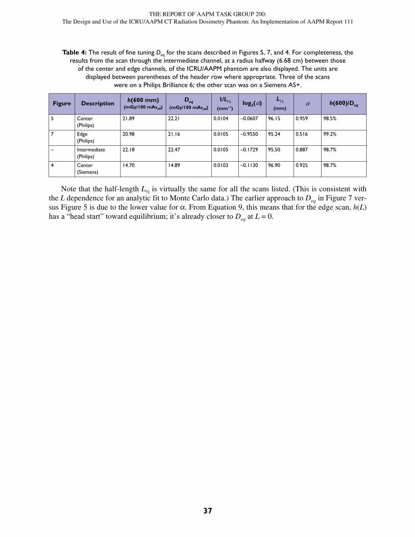
This analysis was repeated for several more scans with the results listed in Table 4. The corre-sponding figure for each row of data is given in the first column: Figure 5 for the data just described,Figure 7 for the edge data, and Figure 4 for the data acquired on a Siemens AS+ scanner. For com-pleteness, the data acquired by scanning through the intermediate channel of the phantom is alsoshown (but with no corresponding figure). This intermediate channel is at a radius of 6.68 cm.

(14)h L L( ) . . .( / . ) 22 21 1 0 959 2 10096 15mGy per mAsmm

eff

Figure 10. A plot of L versus g(L,D*). D* was adjusted to give the best fit to a straight line. This occurs when avalue of 22.21 mGy/100 mAseff is chosen. The curve for D* set to h(600 mm) = 21.9 mGy/100 mAseff is shown forcomparison. The regression line and linear parameters are displayed using Excel’s Trendline tools.

L (mm)0 200 400 600

g(L,

D*)

-8

-6

-4

-2

0

D* = 22.2, R2 = 1(y = -0.0104x - 0.0607)

D* = 21.9, R2 = 0.919


37

Note that the half-length L½ is virtually the same for all the scans listed. (This is consistent withthe L dependence for an analytic fit to Monte Carlo data.) The earlier approach to Deq in Figure 7 ver-sus Figure 5 is due to the lower value for . From Equation 9, this means that for the edge scan, h(L)has a “head start” toward equilibrium; it’s already closer to Deq at L = 0.

Table 4: The result of fine tuning Deq for the scans described in Figures 5, 7, and 4. For completeness, theresults from the scan through the intermediate channel, at a radius halfway (6.68 cm) between those

of the center and edge channels, of the ICRU/AAPM phantom are also displayed. The units aredisplayed between parentheses of the header row where appropriate. Three of the scans

were on a Philips Brilliance 6; the other scan was on a Siemens AS+.

Figure Description h(600 mm)(mGy/100 mAseff)

Deq(mGy/100 mAseff)

1/L½(mm–1)

log2()L½

(mm) h(600)/Deq

5 Center(Philips)

21.89 22.21 0.0104 –0.0607 96.15 0.959 98.5%

7 Edge(Philips)

20.98 21.16 0.0105 –0.9550 95.24 0.516 99.2%

– Intermediate(Philips)

22.18 22.47 0.0105 –0.1729 95.50 0.887 98.7%

4 Center(Siemens)

14.70 14.89 0.0103 –0.1130 96.90 0.925 98.7%

the design and use of the icru/aapm ct radiation dosimetry … · 2020-02-14 · the design and use...

Documents