the development, validation, and integration of aircraft
TRANSCRIPT

The Development, Validation, and
Integration of Aircraft Carrier Airwakes for
Piloted Flight Simulation
Thesis submitted in accordance with the requirements of the University of
Liverpool for the degree of Doctor in Philosophy
by
Michael Francis Kelly
School of Engineering
University of Liverpool
March 2018

i
Abstract
This thesis reports on an investigation into the effects of ship airwake upon
piloted aircraft operating to the United Kingdom’s newly commissioned Queen
Elizabeth Class (QEC) aircraft carriers. Piloted flight simulation has been used to
inform operation of aircraft to the ship, helping to identify potential wind-
speeds/directions requiring high pilot workload prior to First of Class Flight
Trials (FOCFT) aboard HMS Queen Elizabeth.
The air flow over the QEC was generated using full-scale, time-accurate
Computational Fluid Dynamics (CFD) at a range of wind azimuths, with the
resultant airwakes incorporated into the flight simulators at both the University
of Liverpool and BAE Systems Warton, enabling unsteady aerodynamic loads to
be imposed upon rotary-wing and fixed-wing aircraft models, respectively.
An additional CFD airwake was generated around a US Navy LHA helicopter
carrier, and a comparison was made with real-world anemometer data in an
attempt to validate the CFD method used for QEC. LHA at-sea measurements
were found to be unreliable for CFD validation due to the inherent
unpredictability of at-sea testing. As a result, an experimental validation
experiment was recommended to validate the QEC CFD airwakes. A comparison
was made between LHA and QEC, with the twin-island QEC found to have
increased turbulence gradient across the flight deck when compared with the
single-island LHA.
A description is given of the development of a novel Acoustic Doppler
Velocimetry (ADV) experiment in a recirculating water channel, for which a
1:202 scale (1.4m) physical model of QEC was produced. To ensure spatial
accuracy of ADV probe measurements during validation, an electronic,
programmable three degree-of-freedom traverse system has also been
incorporated into the water channel, allowing automated positioning of the ADV
probes along the SRVL glideslope with sub-millimetre accuracy.
Finally, the validated CFD airwakes were incorporated into the HELIFLIGHT-R
piloted flight simulator at Liverpool, for which a QEC simulation environment has
been developed. Two former Royal Navy test pilots then performed a series of
landings to the deck of the QEC in a Sikorsky SH-60 Seahawk, to demonstrate this
newly developed capability at Liverpool, and to provide an initial assessment of
pilot workload in varying wind speeds and azimuths, prior to real-world FOCFTs.
The findings of this initial flight testing is reported in this thesis, as are
conclusions and recommendations for future work.

ii
Acknowledgements
The work reported in this thesis was joint funded by EPSRC and BAE Systems
under an Industrial CASE Award (voucher 12220109). The author is also pleased
to acknowledge the contribution of the IMechE Whitworth Senior Scholarship
Award in supporting this research.
Additional thanks go to ANSYS UK Ltd. for their continued support in the ongoing
research at the University of Liverpool.
Thank you to my supervisors Prof Ieuan Owen and Dr Mark White for your
endless patience and guidance, and to my industrial supervisor Dr Steve Hodge,
without whom this project would not be possible.
Thank you to all my colleagues and friends in the School of Engineering,
particularly Becky Mateer, Jade Adams-White, Wajih Memon, Neale Watson and
Sarah Scott – our shared adventures will be the highlight of my time at Liverpool.
Finally, thank you to my parents Vincent and Marian Kelly for always being there
for me when I need you; I am who I am because of your unconditional love and
support.
This thesis is dedicated to the loving memory of my grandparents Catherine and
Jim Beaman, and Catherine and Frank Kelly.
iii
Table of Contents
Abstract ............................................................................................................................................... i
Acknowledgements ....................................................................................................................... ii
Nomenclature ................................................................................................................................ vii
Abbreviations ................................................................................................................................. ix
Chapter 1 – Introduction and Literature Review .............................................................. 1
1.1 Ship-Air Qualification Testing ....................................................................................... 4
1.2 F-35B QEC Carrier Integration ...................................................................................... 7
1.3 Previous Ship-Air Dynamic Interface Research ................................................... 10
1.3.1 Genesis of Aircraft Carrier Airwake Research .............................................. 11
1.3.2 Empirical Estimations of Carrier Airwake ..................................................... 14
1.3.3 Contemporary Ship Airwake Research ........................................................... 16
1.4 Aims and Objectives ........................................................................................................ 22
1.5 Chapter Summary ............................................................................................................ 23
Chapter 2 – CFD Airwake Generation .................................................................................. 25
2.1 Requirements..................................................................................................................... 25
2.2 CFD Approach .................................................................................................................... 26
2.2.1 Identification of Focus Region ............................................................................ 27
2.2.2 Domain Sizing ............................................................................................................ 28
2.2.3 QEC Geometry and Mesh Generation ............................................................... 29
2.2.4 Wind Azimuth and Magnitude ............................................................................ 31
2.2.5 Atmospheric Boundary Layer ............................................................................. 34

iv
2.3 CFD Solver ........................................................................................................................... 38
2.3.1 CFD Solver Setup ...................................................................................................... 38
2.3.2 Turbulence Modelling ............................................................................................ 42
2.3.3 Numerical Settings .................................................................................................. 43
2.3.4 Time Step Sizing ....................................................................................................... 45
2.4 CFD Execution .................................................................................................................... 46
2.4.1 Initialisation ............................................................................................................... 46
2.4.2 Simulation Settling Period .................................................................................... 47
2.4.3 Airwake Data Export and Interpolation .......................................................... 49
2.5 Initial Visualisation and Discussion of QEC Airwakes ....................................... 49
2.6 Chapter Summary ............................................................................................................ 53
Chapter 3 – CFD Validation Procedure ................................................................................ 54
3.1 USS Peleliu Validation ..................................................................................................... 55
3.1.1 Geometry and Meshing .......................................................................................... 56
3.1.2 Full-Scale Data Format ........................................................................................... 58
3.1.3 Results .......................................................................................................................... 60
3.1.3.1 General Observations .................................................................................... 60
3.1.3.2 Comparison with Experimental Data ...................................................... 61
3.1.3.3 Comparison Between LHA and QEC Airwakes .................................... 67
3.1.4 Summary of LHA CFD Validation ....................................................................... 69
3.2 Water Channel Validation Experiment .................................................................... 70
3.2.1 Rationale for use of a Water Channel ............................................................... 71
3.2.2 QEC Physical Model ................................................................................................. 72
3.2.1.1 Material Selection and Manufacture ....................................................... 74
3.2.2.2 Water Channel Attachment Method ........................................................ 77
3.2.3 Acoustic Doppler Velocimetry ............................................................................ 80
3.2.3.1 ADV Literature Review ................................................................................. 80

v
3.2.3.2 ADV Experimental Procedure .................................................................... 85
3.2.4 ADV Traverse System ............................................................................................. 90
3.2.5 Experimental Validation Results........................................................................ 93
3.2.5.1 SRVL Glideslope ............................................................................................... 95
3.2.6 Expanding the Project ............................................................................................ 98
3.3 Chapter Summary ......................................................................................................... 103
Chapter 4 – Flight Simulator Integration ........................................................................ 105
4.1 HELIFLIGHT-R Flight Simulator .............................................................................. 105
4.2 Aircraft Model ................................................................................................................. 107
4.3 WOD Conditions ............................................................................................................. 109
4.4 CFD Interpolation Sizing ............................................................................................. 112
4.5 HELIFLIGHT-R airwake checks ................................................................................ 114
4.6 Chapter Summary ......................................................................................................... 117
Chapter 5 – Piloted Flight Testing ...................................................................................... 118
5.1 Flight Test Procedure .................................................................................................. 118
5.1.1 Mission Task Elements ....................................................................................... 119
5.1.2 Test Data Recording ............................................................................................. 122
5.2 Flight Trial 1 – Ahead WOD ....................................................................................... 124
5.2.1 Results ....................................................................................................................... 125
5.2.1.1 Spot 5 ................................................................................................................ 127
5.2.1.2 Spot 6 ................................................................................................................ 132
5.3 Flight Trial 2 – Green 25° WOD ................................................................................ 136
5.3.1 Results ....................................................................................................................... 138
5.3.1.1 Spot 1 ................................................................................................................ 140
5.3.1.2 Spot 2 ................................................................................................................ 141
5.3.1.3 Spot 3 ................................................................................................................ 141
5.3.1.4 Spot 4 ................................................................................................................ 142

vi
5.3.1.5 Spot 5 ................................................................................................................ 143
5.4 Chapter Summary ......................................................................................................... 147
Chapter 6 – Conclusions and Recommendations ......................................................... 150
6.1 Conclusions ...................................................................................................................... 150
6.1.1 Aircraft Carrier CFD Generation ..................................................................... 150
6.1.2 Experimental Validation .................................................................................... 151
6.1.3 QEC Rotary-Wing Flight Testing ..................................................................... 152
6.1.4 General Conclusions ............................................................................................. 153
6.2 Recommendations ........................................................................................................ 154
References ................................................................................................................................... 156
Appendix A: Publications....................................................................................................... 177

vii
Nomenclature
Roman Notation
A Cross-sectional area m2
Aship Ship cross-sectional area m2
Atunnel Working section cross-sectional area m2
B Beam, ship m
C Courant number
D Draft, ship m
d Uniform depth m
f Frequency Hz
Fr Froude number
g Acceleration due to gravity m/s2
Hdeck Height of QEC flight deck, 18.3m ASL m
k Turbulent kinetic energy J/kg
l Turbulent length scale m
L Characteristic length m
ṁ Mass flow rate kg/s
N Number of samples
Smax Maximum allowable model scale
St Strouhal number
tset Estimated CFD settling time s
u Velocity in x direction m/s
𝑢∗ Friction velocity m/s
v Velocity in y direction m/s
V Velocity m/s
V1 Wind speed measured at height z1 m/s

viii
Vfs Freestream velocity m/s
Vinlet Water channel working section inflow velocity m/s
Vref Reference wind speed m/s
Vship Ship forward speed kt
Vwind Natural wind speed kt
Vwod Relative wind speed over deck kt
vx Vector sum of natural wind and ship speed in x kt
vy Vector sum of natural wind and ship speed in y kt
w Velocity in z direction m/s
W Width m
X Longitudinal distance from ship CG m
Y Lateral distance from ship CG m
Z Height above ASL m
z0 Surface roughness length m
z1 Height at which wind speed V1 is estimated m
zref Height ASL of reference wind speed m
Greek Notation
ω Specific dissipation s-1
δ Boundary layer thickness m
Δt Time-step size s
Δx Computational cell size in x m
Δy Computational cell size in y m
Δz Computational cell size in z m
ε Turbulence dissipation rate J/kg.s
κ Karman constant
ψwod Relative wind heading, relative to ship heading °
ψwind Natural wind heading, relative to ship heading °
α Surface roughness constant
ρ Density kg/m3

ix
Abbreviations
ABL Atmospheric Boundary Layer
ABS Acrylonitrile Butadiene Styrene
ACA Aircraft Carrier Alliance
ACP Aerodynamic Computation Point
ADV Acoustic Doppler Velocimetry
AFDD Aero Flight Dynamics Directorate
AirDyn Airwake Dynamometer
AO Auxiliary Oiler
ART Advanced Rotorcraft Technology Inc.
ASCII American Standard Code for Information Interchange
ASL Above Sea Level
ASTOVL Advanced Short Take Off and Vertical Landing
BAES BAE Systems
BSPT British Standard Pipe Thread
CASE Collaborative Award in Science and Engineering
CAUM Corrected All Up Mass
CFD Computational Fluid Dynamics
CFL Courant-Friedrichs-Lewy condition
CG Centre of Gravity
CIWS Close-In Weapon System
CPU Central Processing Unit
CRADA Cooperative Research and Development Agreement
CV Carrier Variant
CVN US Navy aircraft carrier, nuclear powered
DDES Delayed Detached Eddy Simulation

x
DDR Double Data Rate
DERA Defence Evaluation and Research Agency
DES Detached Eddy Simulation
DI Dynamic Interface
DIPES Deck Interface Pilot Effort Scale
DMLS Direct Metal Laser Sintering
EPDM Ethylene Propylene Diene Monomer
EPSRC Engineering and Physical Sciences Research Council
FDM Fused Deposition Modelling
FHFA Flying Hot Film Anemometry
FLYCO Flying Control
FOCFT First of Class Flight Trials
FS&T Flight Science and Technology research group
GIS Grid Induced Separation
HPC High Performance Computer
ILES Implicit Large Eddy Simulation
LCD Liquid Crystal Display
LCoS Liquid Crystal on Silicon
LDV Laser Doppler Velocimetry
LES Large Eddy Simulation
LHA Landing Helicopter Assault
LHA-5 USS Peleliu
LSO Landing Signals Officer
MILES Monotone Integrated Large Eddy Simulation
MOD UK Ministry of Defence
MoU Memorandum of Understanding
MTE Mission Task Element
MUSCL Monotonic Upwind Scheme for Conservation Laws
NATO North Atlantic Treaty Organisation
NAVAIR US Naval Air Systems Command
NIWA New Zealand Institute for Water and Atmospheric Research
NLDE Non-Linear Disturbance Equations
xi
NPL National Physical Laboratory
NRC National Research Council Canada
PBCS Pressure-Based Coupled Solver
PBNS Pressure-Based Navier-Stokes
PUR Polyurethane
QEC Queen Elizabeth Class
RANS Reynolds Averaged Navier-Stokes
RFA Royal Fleet Auxiliary
RMS Root Mean Square
RN Royal Navy
SDRAM Synchronous Dynamic Random Access Memory
SFS Simple Frigate Shape
SGS Sub-Grid Scale
SHOL Ship Helicopter Operating Limits
SHWA Stationary Hot Wire Anemometry
SNR Signal-to-Noise Ratio
SRS Scale-Resolving Simulation
SRVL Shipborne Rolling Vertical Landing
SSD Solid State Disk
SST Shear Stress Transport
STL Stereolithography file format
STOVL Short Take Off and Vertical Landing
T23 Type 23 frigate
T26 Type 26 frigate
T45 Type 45 destroyer
TTCP The Technical Cooperation Program
UAV Unmanned Aerial Vehicle
UoL University of Liverpool
URANS Unsteady Reynolds Averaged Navier-Stokes
USB Universal Serial Bus
USN US Navy
VL Vertical Landing

xii
VTOL Vertical Take Off and Landing
WES Waterways Experiment Station
WOD Wind Over Deck

CHAPTER 1 – INTRODUCTION AND LITERATURE REVIEW
1
Chapter 1 – Introduction and Literature Review
Operating aircraft from ships is a highly demanding task for both pilot and
aircraft; in particular, the launch and recovery phases present significant
challenges, for both fixed- and rotary-wing aircraft. Compared to land-based
operations, the ship’s flight deck is small and constantly moving in roll, pitch and
heave. Visual cueing is also often impaired, due to the close proximity of the ship’s
superstructure to the landing spot, sea spray upon the aircraft
windscreen/canopy, and night time operational requirements for reduced levels
of lighting on the flight deck. An additional major challenge is the highly turbulent
air flow around the ship’s superstructure and over the flight deck, which is due
to a combination of the prevailing wind and the ship’s speed. This turbulent flow,
known as the ship’s ‘airwake’, can adversely affect aircraft performance,
disturbing the aircraft’s flight path and requiring immediate corrective action
from the pilot to compensate. Consequently, pilot workload will be increased and
margins for error will be reduced, directly affecting the safe operational envelope
of the combined aircraft/ship system. Even for Advanced Short Take Off &
Vertical Landing (ASTOVL) aircraft with highly-augmented digital Flight Control
Systems (such as the F35-B Lightning II aircraft being acquired as a replacement
for the Harrier), a ship’s airwake could potentially have an undesirable impact
upon the response of the aircraft’s Air Data Systems. Therefore, even advanced
aircraft with generally low pilot workload are not immune to the effects of ship
airwake.
It is highly desirable therefore to have prior knowledge and understanding of the
airwake characteristics before the ship goes to sea. It has traditionally been
common practice for wind tunnel tests to be used to measure the air flow around
a model-scale ship; however, there has been growing confidence in the use of

CHAPTER 1 – INTRODUCTION AND LITERATURE REVIEW
2
computer modelling and Computational Fluid Dynamics (CFD) is now a viable
alternative to wind tunnel testing (as will be demonstrated in this thesis),
particularly as CFD software has become more advanced and computer
resources have become more available and affordable.
Ship airwake models have three important application areas:
1. Ship Design: During the design process, many operational requirements
which affect aircraft launch and recovery are taken into account.
However, this is not the case for the ship’s airwake. The impact of the
ship’s superstructure design on an approaching aircraft is not fully
appreciated until First-of-Class Flight Trials (FOCFT), at which point
either expensive modifications are required or, alternatively, a reduced
operational capability may have to be accepted. High-fidelity simulations
of the aircraft and ship, including the airwake, would provide designers
with a better appreciation of the impact of superstructure design choices
on the aircraft and its systems at an early stage in the design process, thus
avoiding costly ‘surprises’ during qualification testing.
2. First-of-Class Flight Trials: The qualification and clearance of an aircraft to
operate from the deck of a ship is currently achieved through a series of
flight trials, known as First-of-Class Flight Trials. These trials are
expensive, hazardous and time-consuming and their scope is often limited
by the available wind and sea conditions. High-fidelity simulations would
enable some of these trials to be conducted in a piloted flight simulator,
thus reducing time and costs, and increasing safety. Furthermore, since
the simulator provides a safe and controllable environment, testing could
be conducted at the edges of the flight envelope, potentially leading to a
greater operational capability. At the very least test pilots would be better
prepared for the conditions at the ship.
3. Pilot Training: It is generally accepted that pilot training is increasingly
being conducted in high-fidelity full-mission simulators. However, there
is currently no requirement to include a fully validated ship airwake in
current flight simulator training standards, with most training simulators
providing little more than a generic representation of the ship’s airwake.

CHAPTER 1 – INTRODUCTION AND LITERATURE REVIEW
3
This is not an acceptable situation, particularly for single-seat aircraft,
where a pilot may be operating from the ship for the first time on their
own. This issue is made particularly acute in situations where pilots have
not operated from the ship for an extended period, or when introducing a
new pilot or one who is converting from a different type of aircraft, during
currency retraining or building-up a new capability (e.g. introducing a
new ship or aircraft, or using a new recovery technique such as Shipborne
Rolling Vertical Landings (SRVL)). Improving operational safety in these
circumstances is a priority, and high-fidelity flight simulation could play
an important role.
As discussed above, the risks associated with not predicting or fully appreciating
the impact of ship airwake at the design and clearance stages are high. The
potential consequences of costly design changes or limited in-service capability,
of aircraft or ship, to the business and reputation of both the navy and the
equipment manufacturer is a significant consideration. However, the impact of
the ship’s airwake can never be completely mitigated and so the prospect of
developing improved flight simulators, which better prepare pilots for ship
conditions, is an attractive one, and the University of Liverpool (UoL) has been at
the forefront of research in this area, for example in Hodge, et al., (2012). The
University has a number of facilities to support this research, including a multi-
CPU High Performance Computing (HPC) cluster, experimental wind/water
tunnels, and an advanced piloted flight simulation laboratory.
Using its expertise in naval flight simulation, UoL has an established track record
of working with both BAE Systems and the UK Ministry of Defence (MoD) in this
area, providing ship airwake models to the MoD for the Type 23 frigate and the
Wave Class Auxiliary Oiler, in addition to providing airwakes for several
iterations of the evolving Type 26 Global Combat Ship during the design stage.
The tools and techniques used to develop these models at UoL are world-leading,
but they have so far only been applied to “single-spot” ships, which have one
landing spot for rotary-wing operation. Further, experimental validation of the
unsteady airwakes has so far been limited to frigate/destroyer-sized ships, with
CHAPTER 1 – INTRODUCTION AND LITERATURE REVIEW
4
no consideration yet given to fixed-wing operation to a much larger aircraft
carrier.
1.1 Ship-Air Qualification Testing
As part of the preparations for operation of aircraft to a new class of ship,
considerable effort is invested to minimise the risk to life and equipment during
future operational use. A procedure for determining safe operational limits
during take-off/landings has been developed, which allows crews to perform a
risk assessment according to helicopter load, sea state, visibility, and wind
speed/direction. These Ship Helicopter Operating Limits (SHOL) are used to
provide a guide for pilots and crew on identifying the maximum permissible
limits for a given helicopter landing on a given ship deck.
SHOLs are currently determined on behalf of the Royal Navy (RN) by performing
FOCFTs for every possible ship-helicopter combination, using test pilots to
perform numerous landings in a wide range of conditions at sea. During FOCFT
testing, ratings are given by a pilot to each landing, and are assigned according to
perceived workload for an average fleet pilot (Forrest, 2009). The Deck Interface
Pilot Effort Scale (DIPES), a typical pilot rating scale for determining SHOL, is
shown in Fig 1. When producing SHOL diagrams, ratings of 1-3 are deemed
permissible, while ratings of 4-5 are considered outside of safe operating limits.
A rating of 3 can be considered to be the limit of safe operation for a given ship-
helicopter combination, for a fleet pilot of average ability. (Carico, et al., 2003)
Once the pilot rating for each wind speed, direction, and sea state has been
determined using a combination of flight testing and predictive
interpolation/extrapolation, the completed wind envelope for a given ship-
helicopter combination can be produced. An example of an operational SHOL
diagram is shown in Fig 2. As can be seen, the diagram illustrates the safety
boundaries for each wind speed and direction, at a range of Corrected All Up Mass
(CAUM). Maximum permissible deck motion angles are also listed in the SHOL
diagram. It should be noted that “Red” denotes a wind incoming from the port
side of a ship, while “Green” denotes a wind from the starboard side of a ship.

CHAPTER 1 – INTRODUCTION AND LITERATURE REVIEW
5
Fig 1: DIPES rating scale (Carico, et al., 2003)
This method of determining the SHOL for a given ship-aircraft combination, while
reliable, evidently carries numerous practical difficulties. It is clear that this

CHAPTER 1 – INTRODUCTION AND LITERATURE REVIEW
6
FOCFT qualification process will incur considerable expense, with crews and
equipment engaged for several weeks in the task of determining SHOLs for a new
ship-helicopter combination. Even after several weeks at sea, the desired
environmental conditions for determining a complete SHOL might not be
encountered, with crews depending upon the forecast of wind and sea state
within reach of the ship to complete testing. Indeed, helicopter mass is often the
only fully controllable variable during SHOL testing (Carico, et al., 2003). As a
result of this unpredictability, several techniques can be employed to obtain the
required SHOL data for a given ship-helicopter combination. For example, certain
environmental conditions can be altered during testing by changing ship heading
relative to the wind or wave direction; however, these conditions cannot always
be changed independently, and the degree of modification is often limited. Often,
where a full range of conditions are not met at sea, interpolation or extrapolation
of the recorded data must later be performed to obtain a full set of results.
Fig 2: Typical SHOL diagram – UK presentation (Carico, et al., 2003)

CHAPTER 1 – INTRODUCTION AND LITERATURE REVIEW
7
With increasing defence budget constraints now facing many nations, a more
cost-effective method of performing FOCFTs for a given ship-aircraft
combination is desirable. Simulation can offer a cost-effective aid to real-world
SHOL testing, and improvements in simulation are making this option
increasingly more feasible.
1.2 F-35B QEC Carrier Integration
The Queen Elizabeth Class (QEC) aircraft carriers are the largest warships ever
constructed in the UK, and will be three times the size of their RN predecessors,
the Invincible Class aircraft carriers. Having a displacement of 70,600 tonnes,
each ship will provide the UK armed forces with a four-acre military operating
base, which can be deployed anywhere in the world.
BAE Systems is the lead member of the Aircraft Carrier Alliance (ACA), a unique
partnership between BAE Systems, Babcock, Thales, and the MoD, working to
deliver the two QEC aircraft carriers to the RN. HMS Queen Elizabeth, the lead
ship of the class, is currently on-track to be fully operational by 2020, while the
second, HMS Prince of Wales, is, at the time of submission of this thesis, currently
under construction at Rosyth in Scotland and expected to be ready for
deployment in 2023. HMS Queen Elizabeth, which is intended to be the future RN
Flagship, can be seen in Fig 3. The take-off ramp, or ski jump as it is often called,
can be seen at the bow of the aircraft carrier. The unusual twin island
configuration can also be seen, where the forward island is used for ship control,
while the aft island is for flying control (FLYCO). The QEC aircraft carriers have
been designed to accommodate the AW101 Merlin and AW159 Wildcat
helicopters of the Fleet Air Arm and Commando Helicopter Force, in addition to
the Army Air Corps’ AH64 Apache and RAF’s Chinook aircraft. Indeed, both the
QEC hangers and aircraft lifts have been specifically designed to accommodate
Chinook with no blade folding required. With these assets, a flexible combination
of rotary-wing aircraft can be accommodated aboard QEC, providing a platform
that can be adapted to specific mission requirements.

CHAPTER 1 – INTRODUCTION AND LITERATURE REVIEW
8
Fig 3: Aircraft carrier HMS Queen Elizabeth underway
However, the chief wartime advantage of an aircraft carrier is in its fixed-wing
complement, and so the primary weapon system to be equipped aboard QEC will
be the highly augmented Advanced Short Take-Off and Vertical Landing
(ASTOVL) variant of the Lockheed Martin F-35 Lightning II fighter aircraft
(Bevilaqua, 2009). F-35 is the world’s largest defence program in terms of cost,
with Lockheed Martin the prime contractor, while BAE Systems and Northrop
Grumman are Tier 1 partners in the delivery of this fifth-generation multi-role
fighter. One of BAE Systems’ primary responsibilities is the integration of the F-
35B with the UKs new QEC carriers. The ASTOVL version of F-35, known as F-
35B, is being developed concurrently with the QEC program, presenting a unique
opportunity to optimise the air-ship interface and maximise the combined
capabilities of these two assets (Lison, 2009). The F-35A is a conventional take-
off and landing variant, while the F-35C is the carrier variant that uses catapult
and arrestor wires (cats and traps). The F-35B variant employs ASTOVL, with
take-off from QEC also aided by the ski-jump.
While the parallel development of QEC and F-35B presents an opportunity to
optimise integration, there is also considerable uncertainty in the incorporation
of these two multi-billion pound projects as neither QEC nor F-35B has yet (at the

CHAPTER 1 – INTRODUCTION AND LITERATURE REVIEW
9
time of writing) been fully cleared for operational use. In particular, it is not fully
understood how F-35B will perform in the complex airwake of the QEC while at
sea and, therefore, the impact this will have on the cleared flight envelope and
hence operational availability is as yet unknown. This uncertainty also has
implications on pilot training for a single-seat aircraft, where the first time that
the pilot experiences the airwake will be during their first sortie to the ship
without the presence of an experienced instructor. Furthermore, while the UK
has significant legacy experience of shipborne STOVL operation to ships, due to
the retirement of the Harrier fleet from RN service in 2010, recent operational
experience has been largely limited to rotary-wing operation to ships, creating a
shortage of experienced RN crew.
To address the uncertainty around fixed- and rotary-wing operations to QEC, it
is intended that piloted flight simulation be used to de-risk FOCFT, provide a
platform for high-fidelity QEC pilot and aircrew training, and inform future
operational use of aircraft to the ship. In this endeavour, a £2 million dedicated
F-35B/QEC carrier simulation facility has been created by BAE Systems at
Warton in Lancashire, with the purpose of de-risking future flight trials,
informing operational procedure, and providing a high fidelity synthetic test
environment for both pilots and crew. The F-35B/QEC simulation environment
at Warton incorporates a realistic F-35B cockpit mounted in a six-degree-of-
freedom motion base, a ship visual model (including accurate deck markings and
visual landing aids), ship motions up to sea state 6 (taken from QEC
hydrodynamic model testing), and a mathematical flight dynamics model of the
F-35B. Additionally, a QEC Flying Control (FLYCO) simulation has also been
produced, and incorporated into the same virtual world as the simulator used by
the test pilot, allowing the Landing Signals Officer (LSO) to sit at an accurate
representation of their workstation aboard the ship, and interact in real time
with the pilot during a simulated landing. The F-35B simulator and LSO station
are shown in Fig 4.
Perhaps the most critical aspect of an accurate piloted flight simulation
environment around the QEC aircraft carriers is the inclusion of a set of high-
fidelity simulated ship airwakes, created using advanced unsteady CFD. BAE

CHAPTER 1 – INTRODUCTION AND LITERATURE REVIEW
10
Systems is therefore leveraging the considerable research experience of UoL in
this area to develop, validate, and integrate a range of airwakes for QEC into the
flight simulation facility at Warton. This work has been carried out under an
Industrial CASE Award, joint funded by BAE Systems and The Engineering and
Physical Sciences Research Council (EPSRC), and pursued via the PhD project
described in this thesis.
Fig 4: F-35B Simulation Facility at BAE Systems Warton, clockwise from top left: six
degree-of-freedom motion base, LSO station, realistic F-35B cockpit and QEC visual
environment (courtesy: BAE Systems)
1.3 Previous Ship-Air Dynamic Interface Research
This section contains a review of the previous studies upon which the research
presented in this thesis is based, allowing the project to be placed in its historical
context. A large body of literature exists in the area of simulating the aircraft-ship

CHAPTER 1 – INTRODUCTION AND LITERATURE REVIEW
11
dynamic interface and in particular the simulation of ship airwakes. The dynamic
interface (DI) is the region over and around the ship’s landing deck where the
dynamics of the moving ship and the unsteady airwake combine to produce a
challenging flying environment for the aircraft and the pilot.
The majority of research related to the simulation of aircraft carrier airwakes, as
opposed to single-spot combat ships, originated at the US Naval Air Systems
Command (NAVAIR), with significant research effort invested in this field by the
US Navy, which has a large fleet of aircraft carriers including eleven nuclear-
powered supercarriers, in addition to a further nine large amphibious assault
ships in active service.
Topics covered as part of this literature review include general airwake
simulation and flow phenomena analysis, piloted flight simulation, ship-
helicopter qualification testing, and use of CFD to improve ship superstructure
aerodynamics during the design stage.
1.3.1 Genesis of Aircraft Carrier Airwake Research
The potential impact of a ship’s turbulent airwake upon naval aviation has been
apparent since the earliest days of aircraft operation to ships, from the first
successful landings to a moving ship performed by Squadron Commander E.H.
Dunning to HMS Furious in August 1917. HMS Furious was a modified
battlecruiser, fitted with a 49 metre flight deck over her forecastle, and with the
ship superstructure located amidships. During his third landing attempt to the
ship, a sudden and unexpected updraft caught Dunning’s port wing, rolling his
Sopworth Pup overboard and killing him (Gilbert, 2004). This fatal accident, after
just the third successful landing of an aircraft to a moving ship, demonstrated to
the Admiralty the critical importance of ship airwake upon flight safety during
operation at sea. In light of this incident, it was recommended that a second
landing-on flight deck be installed at the aft end of the ship to simplify the landing
procedure, with the forward deck used exclusively for take-off. These
modifications were completed in 1918, and views of the topside arrangement of
HMS Furious after the refit can be seen in Fig 5.

CHAPTER 1 – INTRODUCTION AND LITERATURE REVIEW
12
Despite the modifications to HMS Furious, landing to the ship remained a
hazardous task due to the highly turbulent airwake shedding from the ship’s
large superstructure and passing over the flight decks. To address this,
aerodynamic experiments were performed by the National Physical Laboratory
(NPL), who recommended that Furious be converted to a full-length, flat-deck
aircraft carrier; this refit was carried out between June 1921 and September
1925, and can be seen in Fig 6 (Burt, 1993). Two other notable outcomes of the
research conducted by the NPL aboard Furious were the first examples of
arrestor wires aboard a ship, and the introduction of rounding along the forward
and stern edges of the flight deck. This rounding of the flight deck edges was
demonstrated during experiments to steady the airflow in the lee of the ship, thus
increasing the safety of landing, and can be seen in Fig 6. (Darling, 2009)
Fig 5: Views of HMS Furious circa 1918, fitted with separate fore and aft flight decks
divided by the ship’s large superstructure
The lessons learned from HMS Furious on the negative effects of superstructure
aerodynamics upon aircraft landings were applied in HMS Argus, the first full-
length, flat-deck aircraft carrier, commissioned in 1918. HMS Argus can be seen
in Fig 7. As work on Argus was commenced prior to the sea trial lessons gained
aboard Furious, Argus was originally intended to have twin islands, located on
the port and starboard edges of the ship, and with the flight deck running
between them. Additionally, it was intended that the islands would be connected
by braces, with the ship’s bridge mounted atop this bracing, at 6.1 metres height
above the flight deck. During the design of Argus, further wind tunnel tests were
performed at the NPL to determine the effect of this superstructure design upon

CHAPTER 1 – INTRODUCTION AND LITERATURE REVIEW
13
aircraft during take-off and landing to the ship. Although the twin-island
superstructure was found to significantly increase levels of turbulence passing
over the flight deck, these findings were largely ignored when they were
presented in mid-1917. It was not until the experience of the persistent airwake
problems aboard Furious that all superstructure above flight deck level on Argus
was deleted, very late in the build of Argus in April 1918. (Friedman, 1988)
Fig 6: HMS Furious after 1925 refit, with full-length flight deck. Fore (bottom, left) and
aft (bottom, right) flight deck rounds were fitted to reduce ship airwake turbulence
Although HMS Argus was commissioned too late to participate in the First World
War, the ship was used extensively by the Royal Navy and the NPL as a test bed
for development of future aircraft carrier design and operation. Notably, Argus
was fitted with a dummy island and smoke generators as part of aerodynamic
design optimisation for HMS Hermes, with Hermes finally commissioned in 1924
having a single island after extensive design changes. It was in this way that

CHAPTER 1 – INTRODUCTION AND LITERATURE REVIEW
14
aerodynamic investigation of turbulent ship airwake set the template for aircraft
carrier designs for the next 90 years, with Hermes, shown in Fig 8, entering
service having a hurricane bow, longitudinal arresting gear, two aircraft lifts, and
a characteristic island offset to starboard. (Darling, 2009)
Fig 7: HMS Argus circa 1918, featuring full-length flight deck and no superstructure to
reduce turbulence over the flight deck
Fig 8: HMS Hermes, circa 1931
1.3.2 Empirical Estimations of Carrier Airwake
Given the challenges faced by pilots performing landings to early aircraft carriers,
incorporation of airwake into flight simulators was understood as critical to the
fidelity of a carrier simulation. Prior to the advent of high-power computing,

CHAPTER 1 – INTRODUCTION AND LITERATURE REVIEW
15
empirical methods were developed to estimate the influence of aircraft carrier
airwake upon fixed-wing Carrier Variant (CV) trials in flight simulation
environments, allowing engineers to predict the effect of the massively separated
unsteady airwake region in the lee of the ship known as the “burble”. This burble
effect occurs when the aircraft traverses through the unsteady airwake of an
aircraft carrier on approach and is characterised by a sudden downwash
immediately aft of the ship, which causes fixed wing aircraft to lose altitude and
deviate from the desired glideslope during the most critical phase of a landing.
Experienced pilots learn to anticipate this sudden downwash and make
compensatory inputs to the aircraft controls to maintain an accurate glideslope
and reduce the chances of being waved-off by the Landing Signals Officer (LSO)
(Naval Air Systems Command, 2001).
Prior to the development of today’s advanced CFD capabilities, and to assist
engineers in determining the ability of a given aircraft to fly through the aircraft
carrier burble region, Military Specification (MILSPEC) steady wind ratios were
developed, which apply a mean wind velocity to fixed-wing aircraft during a
simulated landing approach (Naval Air Systems Command, 1980). Additionally, a
quasi-random “unsteady” element is also added to give the effect of turbulence.
The MILSPEC burble is shown in Fig 9. As can be seen, a mean velocity is applied
to the simulated aircraft in the u- (longitudinal) and w- (vertical) components of
the flow, subject to a reference velocity, Vref, with the mean velocity varying with
distance from the pitch-centre of the ship. It can be seen that the pilot will begin
to experience the w-component of the MILSPEC burble at 800m (2600ft, 0.5
miles) aft of the ship pitch-centre, while beginning to experience variation in the
mean u-component at 550m (1800ft, 0.34 miles).
Although the MILSPEC Burble provides a useful approximation of the mean flow
velocities experienced by a fixed-wing aircraft passing along the glideslope
during a landing, it was originally developed for use with the CV approach, which
typically traverses along a 3° glideslope during approach to an angled deck. The
applicability of the MILSPEC burble to other forms of approach such as the
proposed SRVL manoeuvre, which traverses along a nominal 7° glideslope, is
uncertain (Hodge & Wilson, 2008). Further, the MILSPEC burble is merely an

CHAPTER 1 – INTRODUCTION AND LITERATURE REVIEW
16
approximation of turbulence downstream of an aircraft carrier, and so airwake
features unique to a particular class of ship will be omitted. The empirical
MILSPEC burble is therefore being superseded by CFD airwake simulation
techniques as powerful computers have become more affordable.
Fig 9: CVA ship burble steady wind ratios (Naval Air Systems Command, 1980)
1.3.3 Contemporary Ship Airwake Research
With the development of various computer-based simulation tools, ship
superstructure design and flight operations are being influenced by these
technologies. Early development in the field of aircraft-ship simulation research
was progressed as part of The Technical Cooperation Program (TTCP), which is
an international collaborative framework for the defence agencies of member
countries to share research progress and to combine research effort. The TTCP
nations are the UK, US, Canada, Australia and New Zealand. Wilkinson, et al.
(1998) reported progress of a collaborative piece of work on what came to be
known as the Simple Frigate Shape (SFS). The SFS is a simplified representation
of the landing deck of a single-spot frigate, allowing early efforts at CFD to be
performed by researchers in an attempt to produce simulated airwakes. The SFS
can be seen as the rear part of the geometry in Fig 10, comprising a hanger, flight
deck, and funnel. A particular benefit of the SFS research was the sharing of the
geometry amongst TTCP researchers, allowing replication and validation of
results to be made between the defence agencies of the different countries.

CHAPTER 1 – INTRODUCTION AND LITERATURE REVIEW
17
Additionally, by performing a comprehensive wind tunnel analysis with which to
compare results, SFS was intended to become a high-quality tool for CFD
validation of member countries. Wilkinson, et al. (1998) outlined the progress of
the UK defence agency, who were using steady-state Euler computations to
produce a flow characterised by the forming of large vortices with clearly defined
separation points; efforts were also underway by the UK to incorporate early
turbulence modelling to the Advanced Flight Simulator at DERA Bedford.
Wilkinson also outlined efforts to perform full-scale airwake measurements
aboard the ships of member countries and discussed the difficulty in predicting
the effects of helicopter downwash on airwakes during piloted flight simulation.
Fig 10: SFS (Simple Frigate Shape) and SFS2 geometries (Roper, et al., 2006)
Also in 1998, Lumsden and Padfield outlined the major challenges faced during
the operation of helicopters to ships. The airwake of the ship superstructure was
found to be a critical factor in the operational difficulty encountered by crews
during landing and take-off, with a particular Royal Fleet Auxilliary (RFA) Wave
Class oiler shown to have one virtually unusable landing spot at most WOD
angles. Other difficulties frequently encountered were also discussed, such as
operating close behind ship hangar faces, which can cause flow recirculation and
re-ingestion of rotor downwash during landing and take-off. Lumsden discussed
the increasing feasibility of helicopter-ship DI simulation, which he felt could be

CHAPTER 1 – INTRODUCTION AND LITERATURE REVIEW
18
exploited to provide pilot training, aiding FOCFTs and informing ship design to
avoid airwake problems such as those encountered by the RFA Wave Class oilers.
Another development in the fidelty of ship-helicopter DI simulation was the SFS
unsteady CFD simulations successfully produced by Liu, et al. (1998) who used
the CFL3d solver to obtain a steady state solution, before using an inviscid
Navier-Stokes solver based upon the Non-Linear Disturbance Equations (NLDE)
to obtain the unsteady components of the airwake. The results offered good
agreement with experimental studies performed by Rhoades and Healey (1992),
although oil-flow visualisations performed by Cheney and Zan (1999) and later
by Zan (2001) showed poor agreement with the unsteady results, perhaps due to
the inviscid nature of the simulation. The unsteady simulation produced by Liu,
et al. (1998) showed large disturbances in the flow over the flight deck of SFS.
In 2000, Reddy, et al. performed steady computations of SFS, using the Fluent
Navier-Stokes solver and the k-Ɛ turbulence model. Results were shown to be
highly sensitive to grid density, particular in regions where vortical flow was
apparent. The computed airwakes showed re-circulation zones and numerous
vortices. Flow features identified by Cheney and Zan (1999) during oil-flow
visualisation experiments were shown to be well represented using this CFD
method.
Also in 2000, Polsky and Bruner published the first of several time-accurate CFD
computations of a Tarawa-Class Landing Helicopter Assault (LHA) ship. This was
the first published attempt at using CFD to simulate the airwake over an aircraft
carrier. Polsky and Bruner used the COBALT Navier-Stokes solver with
Monotone Integrated Large Eddy Simulation (MILES) to perform the simulations.
Model-scale CFD computations were compared with experimental wind tunnel
data, and were shown to offer good agreement between mean velocity
components in most cases. It was observed that the time-averaged unsteady CFD
and steady-state CFD results differed, with the unsteady CFD data offering closer
agreement with experimental data. Polsky and Bruner also observed Reynolds
number independence for the full-scale flow field, and demonstrated that 15kt
and 30kt computations at 330 degrees were almost identical when scaled; this

CHAPTER 1 – INTRODUCTION AND LITERATURE REVIEW
19
meant one wind speed need be computed for each WOD angle, dramatically
reducing the computational effort required to obtain a full set of airwake data
(kt: knot, nautical mile per hour = 0.514m/s). In 2002, Polsky observed that peak
frequencies over LHA Spot 7 were between 0.1-0.5Hz, offering good agreement
with experimental data.
In 2003 and 2004, Lee and Zan performed a wind tunnel study of a rotorless Sea
King helicopter fuselage immersed in the turbulent airwake of a Canadian Patrol
Frigate. Lee and Zan found the ship airwake frequency range which impacts pilot
workload is between 0.2 – 2.0Hz, demonstrating that the peak frequencies earlier
observed by Polsky (2002) would affect helicopter operation to LHA. Lee and Zan
(2004) surmised that frequencies above 2.0Hz would typically be experienced by
a Sea King helicopter as vibration, rather than as disturbances requiring
corrective action by the pilot, while frequencies below 0.2Hz would occur so
gradually that they would not adversely impact workload.
In 2003, Polsky reported an investigation of ships experiencing beam winds. It
was argued that simulated ship airwake studies tended to show decreasing
agreement with experimental data as WOD angles deviated from ahead and
became more oblique. Polsky suggested that this deviation from experimental
data might be a combination of poor mesh quality, lack of Atmospheric Boundary
Layer (ABL), and inaccurate readings from the measurement system used on the
ship. CFD was performed on both the SFS and LHA at a WOD angle of 90 degrees,
with the SFS CFD compared with wind tunnel data and the LHA CFD compared
with full-scale experimental data. Computations were performed in parallel
using grids of between 4 and 7 million cells. A comparison of SFS CFD versus wind
tunnel experimental data showed excellent agreement. Comparison of the LHA
CFD and full-scale experimental data showed that inclusion of an ABL improved
the agreement of the simulation near one landing spot, however satisfactory
agreement could not be reached at another deck spot, despite improvements to
both meshing and model detail. Polsky felt that this lack of agreement between
CFD and experimental results could be due to the lack of turbulence model in the
MILES code, and suggested employing Direct Eddy Simulation (DES) for future
work.

CHAPTER 1 – INTRODUCTION AND LITERATURE REVIEW
20
In 2004, Silva, et al. performed a wind tunnel study of a V-22 VTOL tilt rotor on
the deck of a LHA carrier in a variety of WOD angles. Silva observed numerous
flow characteristics of LHA, in particular an increased lift over deck edges
thought to be caused by flow seperation, and a strong vortex which passed over
the entire flight deck when the LHA was positioned at a Red 15° WOD angle.
In 2004, Czerwiec and Polsky performed investigations into the effect of a bow
flap on the flow seperation characteristics of an LHA in a headwind. It was
demonstrated that the addition of a flap over the bow significantly reduced the
length of the separation zone and subsequent turbulence. It was discovered that
a more refined mesh was needed in the bow region to obtain good fidelity with
wind tunnel results. In 2004 and further in 2008, Polsky and Ghee analysed the
effects of very small features such as railings and antenna masts upon the fidelity
of CFD data. Results showed good agreement with turbulence aft of the model,
however power spectral density results showed less clear agreement. It was
demonstrated that mesh density, time-step, and longer time-histories are
important to the fidelity of CFD in comparison with model-scale spectral data. It
was concluded that the “sub-grid scale” method of modelling small features was
suitable for approximating first-order effects.
In 2005, Zan produced a comprehensive review of the current state-of-the-art in
the simulation of the ship-helicopter DI. Zan acknowledged that both
experimental and CFD approaches to airwake modelling had much to offer, with
the simulated ship-helicopter DI being particularly well suited to pilot training,
even if it was not yet suitable for SHOL determination. Zan argued that a key
challenge for future airwake simulation was the superstructure effects of ships
designed for “stealth” , and the application of current simulation knowledge to
the operation of UAVs from ships.
Also in 2005, Shipman, et al. performed a study to determine the effects of model
detail on the fidelity of CFD results for the air flow over an aircraft carrier. CFD
and wind tunnel tests were performed upon both a high- and low-fidelity model
of a US Navy Nimitz Class aircraft carrier. It was shown that immediately
downstream of the island, the simplified model had a significantly higher
turbulence intensity. It was suggested that the inclusion of finer detail on aircraft

CHAPTER 1 – INTRODUCTION AND LITERATURE REVIEW
21
carrier towers could help to break up larger scale vortices into smaller ones, thus
reducing the impact of the flow turbulence on an airrcraft. Shipman concluded
that the increased cost in simulation time should be weighed against the likely
increase in accuracy of the solutions.
At UoL, Roper, et al., (2005) and Roper (2006) developed a method to simulate
steady airflow over the SFS and SFS2 geometries (see Fig 10), using the Fluent
solver. The CFD airwakes offered good agreement with previous experimental
work performed by Cheney and Zan (1999). These validated airwakes were then
used by Roper (2006) to populate look-up tables, and were incorporated into the
University of Liverpool’s HELIFLIGHT full-motion flight simulator. Piloted flight
simulation was then performed to produce a steady-state SHOL diagram for a
SFS2/Augusta Westland Lynx combination. Although steady-state airflow was
felt to be present, the pilot workload was deemed to be too low due to the lack of
unsteadiness in the simulated airwakes. For this reason, inviscid unsteady CFD
was later used to produce unsteady airwakes for flight simulation by Hodge, et
al., (2009), although short time-histories were used due to the excessive
computational time required for the unsteady calculations.
In 2010, Forrest and Owen used Fluent with the Detached Eddy Simulation (DES)
method to produce a set of unsteady airwake data for a Type-23 frigate. The CFD
results were compared with at-sea air velocity measurements, and were shown
to have good agreement in both the mean and RMS velocities. Further
improvements were achieved by including the ABL in simulations. It was also
noted that time-accurate CFD airwake modelling had significant effects upon
simulated SHOL envelopes.
Kääriä, et al., (2012) and Kääriä, et al., (2013) outlined the development of an
experimental technique, known as the Airwake Dynamometer (AirDyn), to better
understand the dynamic relationship between ship superstructure and
helicopter rotor loadings. The AirDyn was shown to be an effective tool for
characterising the unsteady loading of a model helicopter in a ship airwake, and
was demonstrated to agree well with qualitative at-sea and simulated flying
experience for a range of WOD angles and ship geometries. Several modifications
were applied to a simplified ship geometry, with the effect of reducing the

CHAPTER 1 – INTRODUCTION AND LITERATURE REVIEW
22
unsteady aerodynamic loads on the helicopter model. Kääriä highlighted the
need for better guidance in the design of warship superstructures to minimise
adverse airwakes at different WOD angles. Kääriä also highlighted that further
work needed to be undertaken to allow helicopter rotors to influence the airwake
of ships in CFD simulations.
1.4 Aims and Objectives
The overall aim of the project reported in this thesis was to develop a set of
validated simulations of the air flow around the QEC aircraft carriers at a range
of wind speeds and angles over deck, and successfully integrate these airwakes
into both the HELIFLIGHT-R flight simulator at Liverpool (White, et al., 2012),
and the F-35B QEC simulation facility at BAE Systems Warton (Atkinson, et al.,
2013). Once successfully integrated, the QEC simulation environments will then
be used in preparations for FOCFTs to the ships, and later to inform future QEC
landing procedures and aid pilot and crew training prior to operational
deployment of HMS Queen Elizabeth in 2020.
The objectives of the project were to develop the following:
Advanced CFD tools and techniques specific to the creation of very large
unsteady aircraft carrier airwakes;
A method to validate the generated airwakes using a combination of
experimental techniques and full-scale experimental data to provide
confidence in the solution;
A procedure for integrating the ship airwake models with a range of
aircraft flight mechanics models in the piloted flight simulation facilities
at both Liverpool and BAE Systems Warton; and to
Demonstrate this newly developed capability by performing an initial
rotary-wing flight trial to QEC using the HELIFLIGHT-R flight simulator,
prior to execution of full-scale at-sea FOCFT.
The flow diagram shown in Fig 11 was used from the outset as a guide to meet
the project’s objectives, and the general layout of this thesis is reflected as such.
As can be seen in Fig 11, validation was pursued using a two-pronged approach,

CHAPTER 1 – INTRODUCTION AND LITERATURE REVIEW
23
with the first stage using full-scale at-sea anemometer data from a US Navy
helicopter carrier to perform a comparison with CFD for this ship, generated
using the method intended for the final QEC airwakes described in Chapter 2. The
second stage of validation was performed using experimental measurements
obtained in the UoL recirculating water channel, described in Chapter 3. Once a
satisfactory comparison was obtained between at-sea anemometer data,
experimental water channel data, and CFD, the integration of these airwakes into
the flight simulators was carried out (described in Chapter 4), and an initial flight
trial was performed, described in Chapter 5.
Fig 11: Flow diagram for the QEC research project
With modelling, validation, and integration of the airwakes completed, a full set
of airwakes was then created on behalf of BAE for their ongoing programme of
simulated FOCFTs that are being performed in the F-35B flight simulation facility
at BAE Systems Warton.
1.5 Chapter Summary
Understanding and mitigating the airwake characteristics of ships, and aircraft
carriers particularly, for aircraft operations has been shown to have been an

CHAPTER 1 – INTRODUCTION AND LITERATURE REVIEW
24
important consideration since the beginning of naval flying operations.
Development of both ship airwake and flight simulation in the latter half of the
21st Century has enabled engineers to better understand the air flow over a ship,
and to prepare for FOCFT trials using flight simulation to both reduce cost and
risk by minimising time spent at sea dedicated to trials. While much international
research effort has been spent on simulation of the aircraft-ship dynamic
interface, there are still several areas of future research to be investigated in an
effort to improve the fidelity of flight simulation. In particular, the development
of synthetic ship airwakes for STOVL flight simulation has received little
published research effort to date. There is therefore a requirement for the
development of CFD airwakes for the purpose of STOVL flight trials to an aircraft
carrier, in tandem with development of an experimental procedure to validate
this new class of CFD airwake.

CHAPTER 2 – CFD AIRWAKE GENERATION
25
Chapter 2 – CFD Airwake Generation
This chapter gives details of the CFD approach used to compute a set of realistic
full-scale airwakes around the QEC aircraft carriers for the purpose of fixed-wing
and rotary-wing piloted flight simulation. The mathematical methods and
approach used are described and justified for this application.
2.1 Requirements
CFD airwakes were to be generated for the QEC aircraft carriers to be
incorporated into both the fixed-wing ASTOVL F-35B Lightning II piloted flight
simulator at BAE Systems Warton, and the HELIFLIGHT-R flight simulator at the
UoL’s School of Engineering for rotary-wing applications. The computed
airwakes must meet the differing requirements of these two simulation facilities,
with several end-user requirements placed upon the finished product. Prior to
the development of a solution strategy, it was first necessary to decide upon what
these requirements were and quantify them where possible to enable a better
understanding of how successfully these requirements were met by each
iteration of the CFD solution. The primary requirements for the CFD solution
were as follows:
The computed airwake simulations must be transient (i.e. changing with
respect to time) as recommended by Roper (2006), and able to accurately
simulate the unsteady ship airwake at the frequency range 0.2 – 2.0 Hz,
for any wind passing over the ship in a 360° range of azimuths (Lee & Zan,
2003) (Lee & Zan, 2004).
The CFD “focus region” must encompass operation of the fixed-wing F-
35B Lightning II fighter aircraft to the ship, resolving turbulent free shear
flow to an acceptable distance for flight operations; this includes: take-off,

CHAPTER 2 – CFD AIRWAKE GENERATION
26
wave-off, VL, and the SRVL glideslope. The solution setup should be
optimised to reproduce unsteady airwake throughout this region,
including along the SRVL glideslope at up to 0.25 miles aft of the ship.
Domain boundary sizing and implementation should be sufficient to
prevent spurious boundary effects upon the QEC region of interest, while
inflow and outflow conditions should be demonstrated to approximate an
at-sea ABL. Temporal stability should also be shown, both in terms of
iterative convergence of transient residual RMS error values, and by
observation of solution monitor points to give confidence that mean
variables do not vary significantly with time.
An experimental study of the flow around a QEC aircraft carrier model of
suitable scale must also be carried out to quantify the accuracy of the
computed airwake solution.
A standardised method for conversion of CFD solution data into a format
suitable for incorporation into BAE Systems and UoL flight simulators
must be developed, including procedures for data transfer and storage.
Checks to ensure correct incorporation of CFD airwakes into both flight
simulators must also be developed and performed to ensure the airwake
experienced by the pilots is within an acceptable tolerance of those
computed using HPC at UoL.
2.2 CFD Approach
The Flight Science and Technology (FS&T) research group at UoL has a proven
track record of performing CFD studies around Royal Navy ships for the purpose
of piloted flight simulation, with these previous studies typically performed
around single-spot frigates and destroyers. Building upon this experience, a new
approach was required to meet the demanding requirements of CFD around a
much larger multi-spot aircraft carrier, intended to be used in preparations for
fixed-wing and rotary-wing flight testing to the ship.
The primary difference between CFD generation for a single-spot frigate and CFD
for a multi-spot ship is the increased cell count required for the multi-spot
computational grid. To adequately resolve the turbulent eddies passing over a

CHAPTER 2 – CFD AIRWAKE GENERATION
27
ship’s landing spot, it is necessary for the mesh sizing in the region of the spot to
be sufficiently fine to allow the eddies to be resolved. If the mesh size is too coarse
it will be larger than the smallest of the eddies, and so will impact upon the
fidelity of the solution by dampening out the smaller eddies which contribute to
larger eddies, and so resulting in an unphysical dissipation of the turbulent
energy in the region of the landing spot. To prevent the occurrence of this
unphysical dissipation of turbulent energy, it is necessary that the relationship
between mesh density and turbulent length scale is properly understood for any
given CFD problem.
2.2.1 Identification of Focus Region
When setting up a CFD solution for analysis of free shear flow, it is necessary to
identify the region of particular interest that will be the focus of the study. In the
case of CFD for piloted landings to QEC, this “focus region” will be the areas
through which aircraft will pass on approach to the ship during the VL and SRVL
manoeuvres, in addition to take-off and wave-off (i.e. an abortive SRVL landing
attempt). These areas can be seen in Fig 12, where locus plots of fixed-wing
ASTOVL operation around QEC are shown, including VL landings to Spot 3 and
Spot 4, SRVL landings, wave-off, and take-off.
Fig 12: Piloted fixed-wing operation to QEC, including VL, SRVL, take-off, and wave-off

CHAPTER 2 – CFD AIRWAKE GENERATION
28
For the case of CFD generation for SRVL landings to the QEC aircraft carrier, the
focus region will necessarily extend beyond the SRVL glideslope, and up to the
point at which pilots will be expected to begin to experience the airwake from the
ship. Previous studies have indicated CV pilots report beginning to experience
aircraft carrier airwake at up to 800 metres (0.5 miles) away from the ship prior
to landing, with the CV glideslope typically following a 3.5° glideslope (Urnes, et
al., 1981). However, landings to QEC will be performed using the SRVL glideslope,
which follows a 7° glideslope (Atkinson, et al., 2013), and as a result, the SRVL
approach can be estimated to begin to experience turbulence from the ship at half
the distance from a CV approach as the aircraft descends into the wake of the
ship, and thus the resolution of turbulence up to 400 metres (0.25 miles) from
the ship for the QEC CFD airwakes was targeted. For reference, the SRVL
approach to the ship is shown in Fig 12, up to a distance of 400m from the stern.
The VL approaches must also be included in the QEC focus region, where both
rotary-wing and fixed-wing VL landings will be performed to the six primary
landing spots on the deck. For Spots 1-5, along the port side of the flight deck,
aircraft will perform an approach from the port side of the ship as they do for RN
frigates and destroyers, with fixed-wing VL to Spot 3 and Spot 4 shown in Fig 12.
(The distribution of the six landing spots will be illustrated later in Chapter 5). As
can be seen in Fig 12, the test pilots typically begin the traverse across deck from
about 60 metres from the ship centre-line, with one traverse beginning at 100
metres from the ship centre-line. These positions at the port side of the ship will
likely experience turbulence in oblique green (i.e. from starboard) winds, and so
this region to the port side of QEC must be included in the focus region to ensure
resolved turbulence in this region.
2.2.2 Domain Sizing
For the selection of QEC domain size and shape, there were two main
considerations. First, the requirement to produce a 360° WOD around QEC
necessitates a cylindrical domain, as employed by Forrest (2009), allowing any
wind azimuth to be easily imposed upon the ship without the need for labour
intensive re-meshing of the domain that would be required for a more usual

CHAPTER 2 – CFD AIRWAKE GENERATION
29
cuboid domain. Secondly, the domain should be large enough to ensure that the
fluid flow in the focus region is not impacted by spurious effects occurring near
to the domain boundaries.
As the focus region contains the 280 metre ship, 400m SRVL approach behind the
stern, and 100m VL approach over the port side, the domain will necessarily be
large to ensure boundaries are kept at a sufficient distance from these areas to
prevent any interference upon the computed fluid flow. However, a large domain
will not significantly increase the cell count of the mesh as the tetrahedral cells
in the region of the far field will be large (up to 10 metre edge length). The domain
height was set at 0.75 ship length, while radius was set to 4.5 ship length, placing
the ship geometry and focus region at a sufficient distance from far-field
boundaries to avoid interference from non-physical boundary interactions; these
dimensions are consistent with Forrest (2009). The position of QEC geometry
and focus region relative to the far-field boundaries can be seen below in Fig 13.
Fig 13: QEC computational domain dimensions
2.2.3 QEC Geometry and Mesh Generation
Prior to performing the CFD study, it was necessary to produce a suitable 3D CAD
model of QEC using top-side ship’s drawings provided by BAE Systems. With
these drawings, a CAD model was produced, primarily using ANSYS ICEM and
SpaceClaim software. The QEC geometry was intended to accurately recreate the

CHAPTER 2 – CFD AIRWAKE GENERATION
30
ship, while providing a good quality grid with a 30cm surface triangle edge
length, with this edge-length recommended by previous grid-dependence studies
for helicopter-ship CFD (Forrest, 2009). An orthographic projection of the final
QEC geometry, as used for all CFD studies reported in this thesis, is shown in Fig
14.
Fig 14: Orthographic projection of the final QEC Geometry used for CFD studies
To achieve a good quality tetrahedral mesh with a 30cm surface triangle size, QEC
geometry features smaller than 30cm were removed, while some slightly larger
features were also necessarily simplified to meet this aim. As it was intended that
prism layers would be grown from all no-slip ship surfaces, geometry surfaces in
close proximity were also manipulated to ensure fidelity while minimising the
incidence of low quality cells in the prism layer. Surfaces intersecting at acute
angles were found to be particularly susceptible to poor quality prisms, and so
care was taken in the meshing of these areas of the ship. Two examples of how
proximity of geometry can impact upon prism layer growth can be seen in Fig 15;
while geometry intersecting at right-angles can be seen to permit a smooth
transition of each prism layer between intersecting surfaces, geometry surfaces
that come into close contact, having acute angles, will cause the prism layers at

CHAPTER 2 – CFD AIRWAKE GENERATION
31
each surface to interfere with each other, significantly reducing prism quality and
producing pyramids in the worst cases.
Fig 15: Examples of low quality prism layer formation due to geometry proximity,
occurring during USS Peleliu (LHA-5) meshing
Geometry representation was carefully considered during creation of the
complex geometry for CFD meshing, often requiring compromise in the final
geometry to achieve a mesh of sufficient quality. In this way, geometry creation
and mesh generation were part of an iterative process, with the ship geometry
modified to improve mesh quality each time an inferior quality mesh was
generated, until global mesh quality was found to be satisfactory. For the
generation of unstructured tetrahedral grids for ANSYS Fluent, quality should not
be less than 0.3 in the tetrahedral cells, where a perfect cell is defined as being
equilateral, and has a quality equal to 1. Once prism layers are grown from the
no-slip surfaces of the tetrahedral domain, quality below 0.01 should be avoided
in the final discretised grid to avoid poor convergence, and the possibility of grid-
induced inconsistencies in the solution. ANSYS Fluent is intolerant of pyramid
cells, and so they should be avoided when repairing low quality prism cells in the
grid.
2.2.4 Wind Azimuth and Magnitude
Critical to the accuracy of the airwake passing over the ship is the correct
specification of wind speed and direction for a given condition. When specifying
boundary conditions, the inlet velocities (input as an ABL profile in units of Mach

CHAPTER 2 – CFD AIRWAKE GENERATION
32
number) must be specified in addition to the normalised vector components of
the flow. As a complete 360° set of airwakes was intended to be simulated for
QEC (approximately 20 CFD airwakes) and given that each simulated airwake
required approximately one month of wall-clock time to produce, it was
necessary that priority be given to wind conditions deemed to be most important
to the acceptance trials for the F-35B. This allowed flight trials to be performed
upon the highest-priority QEC WODs earlier in the programme, while lower
priority WODs were, and are, still being generated. Airwake priorities were
specified according to the conditions likely to be encountered at sea in an
operational context. At the time of publication of this thesis, 15 QEC WOD
azimuths and magnitudes have been generated, and are shown in Fig 16 as
yellow points.
Fig 16: Examples of WOD azimuths for QEC airwakes
In addition to freestream WOD conditions, the ship speed was also taken into
account when specifying wind speed and direction across the domain. This is
because at sea, an aircraft carrier will ideally be travelling into the wind with
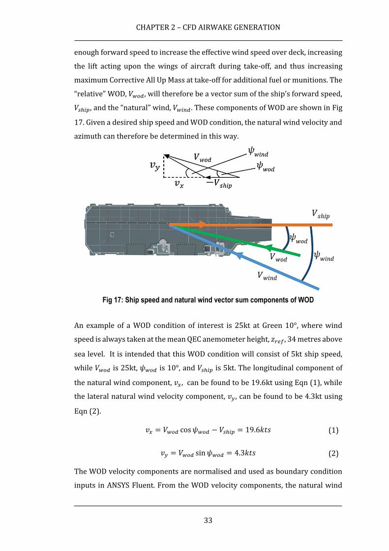
CHAPTER 2 – CFD AIRWAKE GENERATION
33
enough forward speed to increase the effective wind speed over deck, increasing
the lift acting upon the wings of aircraft during take-off, and thus increasing
maximum Corrective All Up Mass at take-off for additional fuel or munitions. The
“relative” WOD, 𝑉𝑤𝑜𝑑, will therefore be a vector sum of the ship’s forward speed,
𝑉𝑠ℎ𝑖𝑝, and the “natural” wind, 𝑉𝑤𝑖𝑛𝑑. These components of WOD are shown in Fig
17. Given a desired ship speed and WOD condition, the natural wind velocity and
azimuth can therefore be determined in this way.
Fig 17: Ship speed and natural wind vector sum components of WOD
An example of a WOD condition of interest is 25kt at Green 10°, where wind
speed is always taken at the mean QEC anemometer height, 𝑧𝑟𝑒𝑓, 34 metres above
sea level. It is intended that this WOD condition will consist of 5kt ship speed,
while 𝑉𝑤𝑜𝑑 is 25kt, 𝜓𝑤𝑜𝑑 is 10°, and 𝑉𝑠ℎ𝑖𝑝 is 5kt. The longitudinal component of
the natural wind component, 𝑣𝑥, can be found to be 19.6kt using Eqn (1), while
the lateral natural wind velocity component, 𝑣𝑦, can be found to be 4.3kt using
Eqn (2).
𝑣𝑥 = 𝑉𝑤𝑜𝑑 cos 𝜓𝑤𝑜𝑑 − 𝑉𝑠ℎ𝑖𝑝 = 19.6𝑘𝑡𝑠 (1)
𝑣𝑦 = 𝑉𝑤𝑜𝑑 sin 𝜓𝑤𝑜𝑑 = 4.3𝑘𝑡𝑠 (2)
The WOD velocity components are normalised and used as boundary condition
inputs in ANSYS Fluent. From the WOD velocity components, the natural wind

CHAPTER 2 – CFD AIRWAKE GENERATION
34
speed and azimuth can also be determined using Eqn (3) and Eqn (4),
respectively, to determine the ambient conditions for a given ship speed and
WOD.
𝑉𝑤𝑖𝑛𝑑 = √𝑣𝑥2 + 𝑣𝑦
2 = 20.1𝑘𝑡𝑠 (3)
𝜓𝑤𝑖𝑛𝑑 = tan−1(𝑣𝑦 𝑣𝑥⁄ ) = 12.5° (4)
2.2.5 Atmospheric Boundary Layer
Accurate modelling of boundary layer formation is known to be critical to the
fidelity of CFD simulations involving turbulent flow. This is because without the
sudden variation in flow velocity near walls, vorticity cannot be generated in the
absence of density fluctuations. Wall bounded flows exist at all scales, with the
largest boundary layer heights forming the lowest part of the Earth’s atmosphere,
the ABL. As with smaller scale wall-bounded flows, the behaviour of the ABL is
directly affected by its contact with the surface of the Earth, and in oceanic
conditions will typically have a boundary layer height of 213m above sea level
(Chen & Lui, 2005). A representation of an at-sea ABL is shown superimposed
over CFD generated for QEC for Ahead WOD in Fig 18. As can be seen from Fig 18,
the reference anemometer height is taken as the mean height of the ships’ three
primary anemometers. Previous research has demonstrated the importance of
correctly modelling this ABL in ensuring the fidelity of CFD for ship airwake
simulations (Healey, 1991).
For the QEC CFD, the increase in wind speed with height inside the oceanic ABL
was varied using the logarithmic profile shown in Eqn (5), where a single
reference velocity, Vref, at a given height, zref, is known. This ABL equation used
for the QEC CFD was obtained from Prandtl’s Law of the Wall divided by itself
(the derivation of which is given in, for example, Blakander and Tennekes (1968),
Wieringa and Rijkoort (1983), and Garratt (1992)).

CHAPTER 2 – CFD AIRWAKE GENERATION
35
Fig 18: Example of an at-sea Atmospheric Boundary Layer
𝑉1 = 𝑉𝑟𝑒𝑓 (𝑙𝑛(
𝑧1𝑧0
)
𝑙𝑛(𝑧𝑟𝑒𝑓
𝑧0)) (5)
Prandtl’s Law of the Wall is represented by Eqn (6), yielding a profile of velocity,
V, at any given height, z. This logarithmic velocity law has been validated for large
Reynolds number wind-tunnel flows for both aerodynamically smooth and rough
cases (in Hinze (1975), and Schlichting (1979)), and has also been validated for
prediction of atmospheric boundary layer for true neutral conditions (Plate,
1971).
𝑉 =𝑢∗
𝜅ln (
𝑧
𝑧0) (6)
Taking Eqn (6), and dividing an unknown velocity, V1, at a chosen height, z1, by a
known velocity, Vref, will cancel out 𝑢∗ (the friction velocity) and 𝜅 (the Karman
constant), as shown in Eqn (7), which can then be rearranged to yield Eqn (5):
𝑉1
𝑉𝑟𝑒𝑓=
ln(𝑧1 𝑧0⁄ )
ln(𝑧𝑟𝑒𝑓 𝑧0⁄ ) (7)
Note that the sea surface roughness length, z0, is the theoretical height at which
horizontal wind speed is equal to zero in a logarithmic velocity profile, with

CHAPTER 2 – CFD AIRWAKE GENERATION
36
experiment recommending a value in the order of 10-3m for oceanic conditions
due to the complex interaction between fluid boundaries (Garratt, 1992). As 𝑧0 is
defined as the height of 𝑧1 at which velocity 𝑉1 is equal to zero, its exact value to
close the equations can be obtained from Eqn (8) (Charnock, 1955), where the
surface roughness constant, 𝛼, is 0.013 for oceanic conditions (Smith & Banke,
1975), and acceleration due to gravity, g, is 9.81m/s².
𝑧0 = 𝛼𝑢∗2 𝑔⁄ (8)
𝑢∗ can be determined using Eqn (6) and substituting known values for V and z
(e.g. using values determined experimentally with an anemometer at a known
height). If we substitute V = 12.86m/s (i.e. 25kt) at z = 34m (i.e. QEC mean ship’s
anemometer height), with a “first guess” z0 = 1.0mm, and a Karman-constant
𝜅 =0.41 (Charnock, 1955), Eqn (6) will yield 𝑢∗ = 0.51m/s. It should be noted
that the von Karman constant has been found to be 𝜅 = 0.40 via numerous wind-
tunnel experiments; however atmospheric measurements have found this value
to be in the range 𝜅 = 0.38 – 0.42. Consult the review of Dyer (Dyer, 1972), and
Garratt - Appendix 4 (Garratt, 1992) for more information.
The value obtained for friction velocity 𝑢∗ can now be input into Eqn (8) to yield
a “second guess” of z0 = 0.34mm. Repeating this procedure by using the 2nd
iteration of z0 into Eqn (6), and then inputting the updated 𝑢∗ into Eqn (8), the
solution converges at the 8th iteration z0 = 0.27mm. After the 8th iteration, the
solution of z0 will converge to a tolerance of 10−7m (i.e. it does not change from
iteration 7 to iteration 8), and so z0 was taken as 0.27mm. This value for z0 is in
good agreement with the terrain classification from Davenport (1960) adapted
by Wieringa (1980), by whom a constant value of z0 = 0.2mm was obtained.
However, this value for z0 disagrees slightly with the experimental work of
Miyake, et al., (1970), by whom a constant value for 𝑧0 between 2.0 and 3.0mm
was obtained directly for a sea surface.
For practical purposes, this minor variation of 𝑧0 in the literature is largely due
to the highly changeable conditions at sea, and so z0 was taken to equal 1.0mm
for QEC CFD inlet conditions. The difference between z0 of 1.0mm and 0.27mm
upon the velocity profile is shown in Fig 19. The flow velocity near to the surface

CHAPTER 2 – CFD AIRWAKE GENERATION
37
(z = 0.05m) was found to be 0.90m/s (7.0% freestream velocity) faster for z0 =
0.27mm than for z0 = 1.0mm, due to the effect of surface roughness upon the flow
near to the wall. However, at maximum measured height (z=250m) the flow for
z0 = 1.0mm was found to have a higher velocity than z0 = 0.27mm by 0.28m/s
(2.2% freestream velocity).
The orange horizontal lines shown in Fig 19 indicate the lower and upper vertical
heights at which the velocity difference between the two curves exceeds 1% of
freestream velocity (Vfs =12.86m/s). Between these two orange markers, the
difference in velocity of the curves does not exceed this tolerance, and so can be
deemed to be acceptable. Note that this 1% difference (i.e. ±0.13m/s) was chosen
arbitrarily as one possible indicator of acceptable tolerance. The lower marker
occurs at z = 13.44m, while the upper marker occurs at 88.27m.
Fig 19: Variation in ABL velocities with differing surface roughness heights
It should also be noted z0 will increase with velocity (i.e. a higher velocity and/or
a lower reference height). For z0 = 1.0mm, using a = 0.016 in Eqn (8) will yield u*
= 0.61. Substituting this value into Eqn (6), using k = 0.4, and z1 = 34m, therefore
we determine that z0 =1.0mm when v1 =15.99m/s (31.1kt).

CHAPTER 2 – CFD AIRWAKE GENERATION
38
2.3 CFD Solver
The ANSYS Fluent CFD tool was used for the airwake computations around QEC.
ANSYS Fluent is a well-validated industry solver and is widely used across a
range of CFD and multi-physics applications. ANSYS Fluent is also particularly
well optimised for the running of massively parallel CFD cases using HPC, making
it ideal for use with the very large computational grids required for CFD around
QEC. The FS&T research group has significant experience of using Fluent to
compute unsteady airwake around ships, having a long-standing research
collaboration with ANSYS UK Ltd.
2.3.1 CFD Solver Setup
The collaboration between ANSYS and the Flight Science and Technology
research group began with the work of Roper (2006), who demonstrated the
importance of implementing transient velocity perturbations around the ship for
piloted flight simulation, however the employed realizable k-ε RANS turbulence
model failed to properly satisfy the available validation data. Later work by
Forrest (2009) instead used a Scale Resolving Simulation (SRS) technique known
as Detached Eddy Simulation (DES), which is a hybrid formulation of RANS and
LES. This approach was found to better match experimental data and yielded
more realistic pilot workload ratings for landings to a ship using a flight
simulator.
The advantage of DES is in its ability to fully resolve turbulent length scales above
the grid size using LES, while modelling turbulence with sub-grid length scales
using a RANS Sub-Grid Scale (SGS) model. RANS models are well validated for
simulating wall-bounded flows, where their calibration according to the law-of-
the-wall (and subsequent optimisation for a particular set of problems) allows
for realistic modelling of the boundary layer without the computationally
prohibitive refinement of the grid close to the Kolmogorov microscales, as would
be required for a purely LES-based solution strategy. Unlike RANS, a LES grid
would also need to be close to isotropic in the near-wall region due to the
inherently isotropic nature of turbulence, with a comparison of grid
requirements shown in Fig 20. As can be imagined, for a practical industrial

CHAPTER 2 – CFD AIRWAKE GENERATION
39
geometry such as a 280m ship, while the RANS grid (left) might require several
million cells to mesh the ship surfaces, the isotropic LES grid (right) will likely
require in the order of billions of cells to adequately mesh the whole geometry
and thereby avoid excessive filtering of turbulent length scales in the boundary
layer. Additionally, the LES time-step size would also need to be significantly
refined in tandem with this reduced grid size to maintain the Courant-Friedrichs-
Lewy (CFL) condition (as LES filters SGS turbulence both spatially and
temporally), further increasing computational cost. This is currently the primary
limitation of LES, as the computational power required to resolve the near-wall
region is not yet viable for problems with all but the lowest Reynolds numbers
and simplest geometries (Spalart, et al., 1997).
Fig 20: Comparison of RANS/DES (left) and LES (right) meshes across the near-wall
boundary layer. A grid with a more ambiguous spacing is also shown (bottom), similar
to that used in some regions of the QEC geometry
In the separated region of turbulent flow, however, LES becomes much more
practically applicable, as the dominant turbulent length scales in this region will
be much larger, and so both grid density and time-step size in this region become
more computationally affordable for practical applications. This is advantageous
as, while optimised unsteady RANS models are both well-validated and efficient
in simulating forces (e.g. lift, drag) acting upon complete vehicle configurations,

CHAPTER 2 – CFD AIRWAKE GENERATION
40
LES is well known to be superior in predicting time-accurate turbulent dynamics
of massively separated flow (Menter, et al., 2003) (Strelets, 2001).
The superiority of LES for wind engineering studies is partly because URANS
simulations characteristically produce an unphysical single-mode vortex street
dominated by the Reynolds-averaged turbulent length scale, while an LES
simulation will resolve the complete turbulent spectrum with a full range of
length scales down to the grid size, beyond which scales are disregarded using
low-pass (i.e. high frequency) filtering. These behaviours can be seen in Fig 21,
which compares a URANS (left) and SRS (right) simulated vortex street shedding
from a three-dimensional cylinder. As can be clearly seen, the URANS simulation
will generate an unphysical single-mode wake behind the cylinder, as a result of
the Reynolds averaging process which removes turbulence from the domain. In
contrast, the wake shedding behind the cylinder generated by SRS (right) in Fig
21 shows a wide spectrum of resolved turbulent length scales, as would be
observed in an experimental setting using flow visualisation.
Fig 21: Comparison of RANS (left), and SRS (right) simulations of flow around a 3D
cylinder, Re=106 (ANSYS, 2016)
Additionally, URANS can also be said to be generally more dissipative than LES
(provided a sufficiently refined grid to avoid excessive LES filtering) in massively
separated regions of flow as a result of the Boussinesq hypothesis, which is the
basis for all one and two-equation RANS turbulence models. Analogous with
momentum transfer due to molecular viscosity in gases, the Boussinesq
hypothesis assumes that momentum transfer between turbulent eddies can be
modelled with an effective “eddy viscosity”. While this assumption offers a useful
approximation for many flows, the Boussinesq hypothesis incorrectly assumes

CHAPTER 2 – CFD AIRWAKE GENERATION
41
turbulent diffusion is isotropic (i.e. eddy viscosity is a scalar), and so under-
predicts turbulent stresses in highly unsteady three-dimensional flows, as will be
encountered in high Reynolds number separated flows. This was found to result
in lower than expected pilot workload ratings during flight trials performed by
Roper (2006), who reported a simulated flight trial using ship airwakes produced
with the realizable k-ε URANS turbulence model.
It is clear that for massively separated flow problems the DES hybrid formulation
of RANS and LES, which offers the advantages of each (i.e. where eddies are only
resolved away from the wall, while boundary layers are simulated using a RANS
SGS model), can yield improved resolution of time-accurate separated flow at a
more affordable computational cost than pure LES for practical industrial
applications. However, while DES is intended to treat the entire boundary layer
region with RANS and apply LES to the separated flow region, one consideration
when using this model is in the presence of a “grey area” between these two
regions where DES can exhibit incorrect behaviour due to ambiguous grid
spacing across the boundary layer. This is a well-known feature of DES, having
been described by the first paper outlining DES (Spalart, et al., 1997). The “grey
area” exists where the streamwise grid spacing becomes shorter than the height
of the boundary layer thickness (δ) at a given location, and can cause premature
switching in these areas from RANS to LES inside the boundary layer where the
grid is not sufficiently isotropically refined to support LES content. This can result
in the phenomenon of “grid induced separation” (GIS) which is resultant from
under-resolved Reynolds stresses and thus artificially reduced skin friction at
these unphysical separation points (Menter & Knutz, 2004). An example of an
ambiguously spaced near-wall grid can be seen in comparison with standard
RANS/DES and LES grids in Fig 20. As can be seen, the streamwise grid spacing
for the RANS/DES grid is longer than the boundary layer height, ensuring the DES
scheme does not incorrectly switch to LES inside the boundary layer. This is not
the case for the ambiguous grid, and it is likely that a pure DES scheme will switch
to LES in the upper third of the boundary layer, resulting in incorrect turbulent
behaviour and potentially impacting upon the fidelity of the simulation. For a
highly complex geometry such as a 280-metre-long aircraft carrier, experiencing

CHAPTER 2 – CFD AIRWAKE GENERATION
42
a range of wind azimuths, it is very difficult to ensure that the near-wall grid is
unambiguous everywhere.
To prevent DES from exhibiting incorrect behaviour in the presence of
potentially ambiguous grids, a modification of DES, called Delayed Detached
Eddy Simulation (DDES) was felt to be a better candidate for the simulation of
massively separated flow, and comes strongly recommended over “pure” DES by
Spalart, et al., (2006) for this application. Using DDES, maximum edge length of
cells in the boundary layer region of flow can be as small as one fifth the boundary
layer height, significantly increasing the robustness of the solution without any
negative effects. While, for a bluff frigate or destroyer, Grid Induced Separation
caused by DES will not be expected to impact significantly upon the solution, for
the QEC aircraft carrier, which features an aerodynamic ski-jump ramp and large
flat-plate flight deck, DDES was felt to be more suitable.
2.3.2 Turbulence Modelling
For bluff body aerodynamics, such as in the prediction of unsteady flow around
a ship superstructure, the massively separated airwake shedding from the ship
will be largely independent of the attached flow in the boundary layers near to
its surfaces. Separation will typically occur as a result of flow around the ship’s
sharp-edged geometry, with the character of the associated separated turbulence
largely unaffected by the attached boundary layers, as demonstrated by Shipman,
et al., (2005). As a result, previous studies of ship airwakes have entirely
neglected resolution of these boundary layers, arguing that the impact of the
boundary layers upon the separated flow region does not justify the
computational expensive of refining the grid near to walls (Polsky, 2006). An
example of this approach to ship airwake CFD is presented by Thornber (2010),
where LES was used across the entire domain with an unstructured tetrahedral
grid lacking any near-wall prism layer, with this approach increasingly referred
to as Implicit Large Eddy Simulation (ILES) (that is, the LES filtering is performed
implicitly, recognising that SGS turbulence will be passively dissipated, as
opposed to the more usual explicit filtering employed via an LES filter). While
this approach can provide a good approximation of the massively separated flow

CHAPTER 2 – CFD AIRWAKE GENERATION
43
in the lee of a bluff object such as a frigate (where a sharp edged hangar will
typically be immediately upstream of the helicopter landing spot focus region), a
more complex geometry such as the QEC will have a combination of both bluff
and streamlined features upstream of its focus region, and so accurate prediction
of boundary layers over curved surfaces is more likely to impact upon the
separated flow through which aircraft are required to travel. For an aerofoil-like
shape, such as the QEC ski-jump, the attached boundary layer will typically have
an increased influence upon the unsteady flow separating from the ski-jump and
cascading across the flight deck. This is because the behaviour in the attached
boundary layer will determine the separation point over these aerofoil features,
thereby defining both the size and the character of this separated flow. As a
result, it was considered necessary to carefully simulate the boundary layer
formation across QEC, using DDES.
For the RANS (boundary layer) region of the QEC domain, the k-ω SST turbulence
model was selected. The k-ω SST turbulence model is widely used due to its
robustness and extensive validation in predicting a range of flows, particularly
those possessing adverse pressure gradients (Menter, et al., 2003).
2.3.3 Numerical Settings
As previously outlined, in the LES region of an SRS simulation the majority of the
turbulent spectrum is resolved, down to turbulent length scales near to the grid
edge-length. Below this limit, turbulent energy is dissipated using a subgrid-scale
model, while the eddy viscosity is defined to ensure correct levels of dissipation
at the larger LES length scales. This low-level eddy viscosity in the LES region of
a simulation enables the transfer of turbulent energy from larger eddies into
smaller eddies in a naturalistic way. Critical to this arrangement is the
assumption that all turbulent dissipation is as a result of the LES model, and so
the spatial numerical settings in a simulation must be carefully selected so as to
minimise numerical dissipation relative to the dissipation due to LES eddy
viscosity across the domain. If the numerical scheme is too dissipative, this “false
diffusion” will add to the diffusion due to eddy viscosity defined by LES, and
excessively dampen out turbulence in an unphysical way.

CHAPTER 2 – CFD AIRWAKE GENERATION
44
Another approach is to entirely remove eddy viscosity from the LES subgrid-scale
model and instead provide all turbulent dissipation across the domain as
numerical dissipation via the spatial discretisation scheme; this alternative
method is known as Monotone Integrated Large Eddy Simulation (MILES) (Boris,
et al., 1992). In particular, MILES has been widely used for some years by
research engineers at the US Navy’s NAVAIR for performing wind engineering
simulations around ships (Polsky, 2006). MILES is currently not available in
ANSYS Fluent, which uses the standard approach for generating dissipation using
an LES eddy viscosity model, rather than relying upon numerical dissipation.
In an effort to achieve the low numerical diffusion required when using explicit
LES filtering in ANSYS Fluent, the MUSCL third order discretization scheme was
used for momentum as with previous CFD studies at UoL around ships (Forrest,
2009), owing to its reduced numerical diffusion and therefore spatial accuracy
particularly for highly unsteady three-dimensional flows on unstructured
meshes (ANSYS, 2016).
Spatial discretisation for turbulent kinetic energy (k) and specific turbulence
dissipation rate (ω) are not critical to solution accuracy for DES-based
simulations, with the two-equation turbulence model used by the RANS region of
the grid largely unaltered, while the LES region disregards these values. While
the first order upwind scheme would likely be sufficient for these terms, the
second order upwind scheme was selected for spatial discretisation of these
terms to ensure improved accuracy. Discretisation for pressure was set to the
second order scheme for the same reason.
The Pressure-Based Coupled Solver (PBCS) was used, with momentum and
pressure solved simultaneously at each time-step. The coupled solver was
selected as, although it will typically take longer to compute per iteration, it
typically yields better convergence characteristics when compared with a
segregated approach.
For the evaluation of gradients across unstructured cells in the domain (i.e.
estimating values of a flow property at a cell boundary from the cell’s centre
where values are stored), the Green-Gauss node-based gradient scheme was

CHAPTER 2 – CFD AIRWAKE GENERATION
45
selected, as this scheme is known to be more accurate for unstructured meshes
over complex geometry, where mesh quality might be sub-optimal (ANSYS,
2016). The Green-Gauss node-based gradient scheme preserves second-order
spatial accuracy in the construction of the nodal values from the weighted
average of values at the surrounding cell centres, albeit at a small increase in
computational expense, using the method outlined by Holmes and Connell
(1989), and Rauch, et al., (1992).
2.3.4 Time Step Sizing
Correct time-step sizing is critical in DES-based simulations, to ensure the explicit
subgrid scale filter is not unduly activated in the LES region of the grid. When
determining time-step size for any DES-based simulation, the CFL condition
should be obeyed, with the Courant number not exceeding unity throughout the
LES region of the grid. For the one-dimensional case, Courant number, C, can be
obtained from Eqn (9), where u is the fluid velocity in x, Δt is the time-step size,
and Δx is the cell size in x.
𝐶 =𝑢 ∆𝑡
∆𝑥≤ 1 (9)
The Courant number tells the user how the motion of a fluid relates to the
discretised grid for a given time-step, with C ≤ 1 ensuring that a fluid particle will
not move from more than one cell to another within one time-step. Where C ≥ 1,
a fluid particle will travel through more than one cell in each time-step, negatively
impacting the ability of the solver to achieve a converged solution. In the ANSYS
Fluent pressure-based solver, Courant number is not specified by the user, and
so the correct grid-spacing and time-step size should be specified to ensure the
CFL condition is satisfied throughout the domain. The robust design of Fluent
provides some tolerance for cells with Courant numbers in excess of one,
however this should be avoided where possible as an increased number of sub-
iterations will be required per time-step to achieve a converged solution.
To ensure the CFL condition was obeyed across the QEC domain, it was
considered good practice to aim for a Courant number equal to ½ to provide

CHAPTER 2 – CFD AIRWAKE GENERATION
46
sufficient tolerance for increases in flow velocity near to the ship’s complex
geometry. The optimum time-step for the three-dimensional case was therefore
evaluated using Eqn (10) with preliminary QEC steady-state RANS testing and
found to be approximately Δt = 0.01 seconds for a typical 30kt freestream wind
speed.
𝐶 ≈
∆𝑡
2(
|𝑢𝑥|
∆𝑥+
|𝑢𝑦|
∆𝑦+
|𝑢𝑧|
∆𝑧) ≈ 0.5 (10)
2.4 CFD Execution
The following sections give an outline of how the unsteady CFD airwakes were
produced.
2.4.1 Initialisation
Prior to the running of any SRS solution, it is recommended that a “precursor”
steady state RANS simulation should be completed to aid convergence by
approximating the mean flow across the domain, and so each QEC WOD was
preceded by steady-state RANS computation with this aim (ANSYS, 2016). As for
the RANS region of the DDES solution, the SST k-ω turbulence model was used
for the precursor RANS simulation to maintain consistency in the boundary layer
between the time-averaged initialisation and the unsteady DDES simulation that
would follow. All boundary conditions were kept the same, including the
implementation of the ABL, to facilitate convergence.
As the purpose of the steady-state RANS simulation is to provide an
approximation of flow behaviour in each cell to initialise the unsteady solution,
first order accuracy was sufficient for this purpose. As a result, the 1st Order
Upwind discretization scheme was used for momentum, turbulent kinetic
energy, and specific turbulence dissipation rate, while the Standard scheme was
employed for pressure discretisation. Pressure-velocity coupling was achieved
using the SIMPLEC segregated solver. All other parameters were unchanged from
the DDES simulation, which was to follow.

CHAPTER 2 – CFD AIRWAKE GENERATION
47
The steady-state SST k-ω RANS simulation was run for 3000 iterations to achieve
an acceptable level of convergence, requiring approximately 9.5 wall-clock hours
using 300 cores on UoL’s “Chadwick” HPC cluster. Once completed, synthetic
instantaneous turbulence was added to the steady-state solution to initiate
unsteadiness in the DDES simulation.
2.4.2 Simulation Settling Period
The flight simulation requires a 30 second airwake time history, which is then
looped in the simulation software; however, prior to reaching the desired 30
recorded time history, the CFD calculations must first be permitted to “settle”
into periodic turbulence to ensure a repeatable solution. An increased ship length
results in an increased CFD simulation settling time. As an unsteady solution
begins, the fluid should pass over the length of the ship several times for the flow
to acquire a fully unsteady state. For a 130m long frigate at a wind speed of 40kt,
it will take approximately 15 seconds for the flow to pass over the ship 2.5 times.
For a 280m long aircraft carrier at 25kt, it will take approximately 60 seconds for
the flow to begin to achieve a settled transient solution, requiring several hours
of CPU time per second of CFD simulation. The freestream velocity can be
increased to reduce settling time, provided flow remains incompressible;
however, it is important that the CFL condition is obeyed across the ship,
requiring a compromise between settling time and time-step in the simulation
set-up.
In practice, numerous sampling points were placed throughout the domain, and
were monitored until the mean velocity in three components was seen to
converge. From this experience, Eqn (11) has been adopted as a useful
approximation of the simulation settling period, where tset is the settling time, L
is the characteristic length over which the fluid will pass, and Vwod is the
freestream velocity (with units of m/s).
𝑡𝑠𝑒𝑡 ≈2.5𝐿
𝑉𝑤𝑜𝑑 (11)

CHAPTER 2 – CFD AIRWAKE GENERATION
48
It should be noted that this settling time was used as a rule-of-thumb only, with
actual settling time varying in practice due to a range of factors (e.g. time-step,
iterations per time-step, mesh quality, boundary conditions). The total wall-clock
time required per run was found to be approximately 21.5 days using 256
processors, depending upon settling behaviour for a given wind strength and
direction. A typical wall-clock time required for each period of the solution is
shown in Fig 22, which represents a complete time history of u-velocity at a
sampled point in the QEC airwake for Red 18° at 35kt. It can be seen that the
recorded time history period requires more wall-clock time to complete than the
settling period, despite the settling period representing 38.9 seconds while the
recorded data period represents just 30 seconds; this is due to the large amount
of data recorded during the recorded data period, with a 4.68GB instantaneous
airwake file recorded 25 times per second during this period (751 files, 3.52TB
total).
Fig 22: Time history of u-velocity at a sampled point in QEC airwake for Red 18° case
Also shown in Fig 22 is the 10-second moving average of velocity, which varies
considerably over the first 30 seconds and does not begin to converge until at
least 35 seconds, with the velocity minima/maxima also beginning to display
periodicity after this 35 second point. Using Eqn (11) with a 35kt freestream

CHAPTER 2 – CFD AIRWAKE GENERATION
49
wind speed (18 m/s), the required minimum settling period is expected to be
38.9 seconds, in agreement with this observation of settling at the sampling point
in Fig 22.
2.4.3 Airwake Data Export and Interpolation
Once initialisation and settling of each CFD simulation was completed, the
solution was recorded for a period of time, referred to during this study as the
recorded time history. This recorded data period of the QEC simulation was the
part of the airwake time history to be exported and implemented into the piloted
flight simulators at both UoL and BAE Systems – Warton. Due to both the
significant wall-clock time required per second of simulation time, and the
storage requirements for recording this period (each time step was 4.95GB), it
was important to keep the recorded data period as short as possible without
impacting upon the fidelity of the piloted flight simulation trials. However, while
an excessively long recorded data period will result in increased computational
and data storage requirements, an insufficiently long recorded data history will
fail to capture longer frequency turbulent features of the flow in sufficient
numbers, and so impacting upon the fidelity of the simulated airwake
experienced by test pilots.
2.5 Initial Visualisation and Discussion of QEC Airwakes
With the airwake methodology successfully developed, 15 airwakes were
generated around QEC, at a range of azimuths as outlined previously in Fig 16. A
visualisation of the vortices passing over the flight deck for the Ahead WOD
condition is shown in Fig 23, with vortices identified using isosurfaces of Q-
criterion. As can be seen from Fig 23, the majority of turbulent flow passing over
the flight deck in the Ahead condition is caused by separation from the ship’s twin
islands. Vortices are also formed by separation from the ship’s ski-jump and
forward deck edges, however these vortices can be seen to be typically smaller
than those shedding from the twin islands in the Ahead WOD condition. This is

CHAPTER 2 – CFD AIRWAKE GENERATION
50
partly due to the rounded forward edges and ski-jump of QEC, which encourages
flow to largely remain attached over these surfaces.
Fig 23 Isosurfaces of Q-criterion passing over QEC in the Ahead WOD condition
At all Green WOD azimuths, turbulence across the flight deck was dominated by
flow separation from the ship’s twin islands. The effect of the twin-island
arrangement upon aerodynamics across the flight deck is shown in Fig 24, where
contours of turbulence intensity are overlaid with instantaneous velocity vectors
at five wind azimuths. As can be seen, in the Ahead and Green 10° cases, free
shear flow from the forward island cascades over the aft island and combines
with the aft island’s wake over the stern. However, in the Green 25°, 45° and 90°
cases, the wakes from each island become more independent of each other,
forming separate vortex streets that periodically overlap, with each having its
own cyclical period. This is in contrast to a single-island ship, where the vortex
street in the lee of its island will typically be easier to predict, as can be seen in
Fig 25, where isosurfaces of vorticity for an LHA ship are shown.
The interaction of the two vortex streets shedding from the twin-islands and
cascading across the flight deck is highly complex and periodic, creating
additional uncertainty for piloted flight operations to the ship. When compared
with the aerodynamics around a single-island arrangement, as in Polsky &
Bruner (2001), it has been observed that the flow around a twin-island aircraft
carrier will be more uncertain due to the complex interaction between each

CHAPTER 2 – CFD AIRWAKE GENERATION
51
island’s free shear regions in oblique winds, warranting analysis to better
understand flow behaviour. For this reason, a piloted flight simulation trial was
undertaken during this project to gain an understanding of the potential impact
upon flight operations in Green winds, with this piloted flight trial described in
Chapter 5.
In addition to turbulence over the flight deck originating from the ship’s twin-
islands, as the WOD azimuth becomes increasingly oblique (i.e. beam-wise,
rather than longitudinal winds), separation begins to occur from the sharp
longitudinal edges of the flight deck along the port and starboard sides of the
ship. This is also shown in Fig 24, where instantaneous velocity vectors at five
wind azimuths are plotted over contours of normalised turbulence intensity,
positioned at aircraft hover-height 10 metres above the flight deck. As can be
seen, a distinct region of separation occurs from the starboard deck edge near to
the stern in the Green 45° azimuth, increasing levels of turbulence to
approximately 30% across the starboard landing spot (Spot 6, highlighted in
magenta). In the Green 90° condition, significant flow separation can be seen to
occur from the starboard flight deck edge, with turbulence intensities of up to
45% over both the stern landing spots, and over the ski-jump attributable to
starboard deck edge separation. As a result, it is recommended that where
possible, rounded edges be fitted around the port, starboard, and stern deck
edges of aircraft carriers, as they are for the forward deck edges at present.

CHAPTER 2 – CFD AIRWAKE GENERATION
52
Fig 24 Instantaneous velocity vectors plotted over turbulence intensity contours 10m
above flight deck for Ahead (top), Green 10° (upper middle), Green 25° (middle), Green
45° and Green 90° (bottom) airwakes.
Ahead
Green 10°
Green 25°
Green 90°
Green 45°

CHAPTER 2 – CFD AIRWAKE GENERATION
53
Fig 25 Isosurfaces of vorticity over a single-island LHA ship at Ahead, Red 30°, Red
60°, and Red 90° azimuths (Polsky & Bruner, 2001)
2.6 Chapter Summary
This chapter has described the CFD methodology that has been applied in this
research. To create the unsteady velocity field for use in the piloted simulators it
has been necessary to compute the airwakes over the full-scale ship, and at a
frequency of 100 Hz. This has led to grid sizes of ~120 million cells, total
computational times of 30 days, and total file size per airwake of 4.12 TB. The
CFD requirements have far exceeded those of previous studies where the
airwakes over frigates were calculated and then compared with experimental
data. An initial inspection of QEC aerodynamics was performed, with the effects
of the ship’s twin-island arrangement shown to result in complex flow behaviour
across the flight deck in Green winds. The following chapter describes how
experimental data was obtained to compare with the CFD predictions.

CHAPTER 3 – CFD VALIDATION PROCEDURE
54
Chapter 3 – CFD Validation Procedure
Compared with previous ship airwake studies performed at UoL around single
spot frigates, the primary challenge of generating CFD around an aircraft carrier
is the requirement to capture the carrier burble region, along the fixed-wing
glideslope and up to 400 metres (0.25 miles) aft of the ship. The challenge in
accurately capturing this region of the airwake by minimising turbulent energy
dissipation in the CFD solution necessitates experimental validation to ensure
solution accuracy for this new class of airwake problem. The term “burble” is one
used in naval aviation to describe the turbulent air behind the aircraft carrier,
along the flight path and including the area immediately aft of the ship where
there is a downdraught which is felt by the approaching aircraft and pilot.
This chapter outlines the approach used to obtain the experimental validation
data for the CFD results. The first part of this chapter outlines comparisons made
between a CFD airwake generated around a US Navy helicopter carrier (USS
Peleliu, LHA-5) and over-deck ultrasonic anemometer measurements performed
at sea. The anemometers allowed instantaneous three-component velocities to
be recorded at 20Hz at a range of locations across the flight deck and directly
compared with CFD, the purpose of which was to assist in the development of the
aircraft carrier CFD methodology outlined in Chapter 2, ensuring it was suitable
for a large (250m length) flat-deck ship. The second part of this chapter describes
the design, build, and implementation of a novel Acoustic Doppler Velocimetry
(ADV) experiment in a recirculating water channel, for which a 1:202 scale
(1.4m) physical model of QEC was produced using 3D printing techniques. The
design and installation of an electronic, fully programmable three degree-of-
freedom traverse system is also outlined in this chapter, allowing automated

CHAPTER 3 – CFD VALIDATION PROCEDURE
55
positioning of the ADV probes along the SRVL glideslope with sub-millimetre
accuracy. Comparisons are made between experimental ADV measurements
around the QEC experimental model and CFD results, demonstrating the
suitability of the generated airwakes for use in piloted flight simulation studies.
3.1 USS Peleliu Validation
Prior to performing WOD simulations for QEC, it was decided that the proposed
CFD method would initially be applied to a US Navy LHA ship, specifically USS
Peleliu (LHA-5). LHA-5 was selected for the study due to its comparable size to
QEC, as shown in Fig 26, and due to its similar flat-deck arrangement. Real-world
WOD data was made available for USS Peleliu, with at-sea measurements were
performed by NAVAIR using ultrasonic anemometers in 2000. These
anemometers were used to record three-component velocities at 20Hz across the
flight deck of the ship. The intention was that once a CFD simulation of USS Peleliu
was successfully run, this would allow LHA CFD and NAVAIR experimental
results to be compared, allowing the proposed method for modelling of large
scale aircraft carriers to be validated.
Fig 26: Comparison of QEC and LHA-5 dimensions

CHAPTER 3 – CFD VALIDATION PROCEDURE
56
As with the previously described QEC CFD, a pre-processor, solver, and post-
processor was required to successfully produce an LHA-5 airwake. These would
be ANSYS ICEM, ANSYS Fluent, and ANSYS CFDPost, respectively. Additionally,
Creo Elements/ Pro 5.0 (formerly Pro/Engineer) was used to assist with
geometry modelling, while Tecplot 360 was used to assist with post-processing
of CFD data.
3.1.1 Geometry and Meshing
To successfully produce CFD airwakes for USS Peleliu, an accurate CAD
representation of the ship geometry was needed. USS Peleliu (LHA-5) circa 2000
is shown in Fig 27.
Fig 27: USS Peleliu (LHA-5) at sea, circa 2000
The FS&T research group keeps a catalogue of various ship models for use as
visual representations in the HELIFLIGHT-R flight simulator, as part of which two
LHA models were found in the STL file format which could be used for CFD
meshing. The LHA geometry selected for use offered a very high level of detail,
down to very fine features such as door handles and rivets around windows. This
would clearly be an excessive level of detail for the purposes of CFD for piloted
flight simulation, where a minimum surface mesh size of 30cm was to be used.
Simplification and sealing of the LHA geometry was carried out, with the finished

CHAPTER 3 – CFD VALIDATION PROCEDURE
57
model shown in Fig 28, below. It was necessary to modify the CAD to better
replicate features unique to USS Peleliu, such as removal of the bow guns, and
addition of the Close-In Weapon System (CIWS) tower and radar dome forward
of the main super-structure.
Fig 28: Final LHA geometry used for CFD
Once completed, the geometry was then sealed (i.e. any gaps removed), before
being trimmed at the water line. Finally, the model was placed in a circular prism
domain of 0.75 ship length in height (187.5m) by 4.5 ship lengths diameter
(1125m), to minimise blockage effects and reduce the potential for spurious
effects from far-field boundaries acting upon the ship’s near-field. Although
comparisons were only to be performed at one wind azimuth, a circular prism
domain was used for LHA-5 as to ensure similarity of boundary conditions with
QEC for validation purposes.
Once the LHA-5 geometry was successfully modelled and placed into the
computational domain, a mesh was generated to discretise the domain. The LHA-
5 domain was meshed using an unstructured grid with Delayed Detached Eddy
Simulation (DDES) and the shear stress transport (SST) k – ω turbulence model
employed in the RANS region of the solution, as was done for QEC and described
in Chapter 2.

CHAPTER 3 – CFD VALIDATION PROCEDURE
58
A minimum surface-mesh cell size of 0.3m was specified, allowing structures
such as masts and radomes to be modelled, while ignoring smaller features which
would have little effect upon the LHA-5 airwake in the amplitudes/frequencies
likely to impact upon ship aircraft operations. An unstructured mesh was then
grown from this surface mesh, using a growth function to slowly grow the cell
size from 0.3m at a surface up to a maximum of 10.0m in the far field. A maximum
cell size of 1.0m was specified in the region of interest, near to the ship’s
geometry and encompassing where the NAVAIR anemometer data was recorded;
this approach yielded a total cell count of 52 million cells, while maintaining
similarity with the QEC computational grid.
Boundary surfaces for the LHA-5 geometry were set as no-slip walls, while the
sea surface was specified as a slip wall, preserving the ABL specified at the inlet.
The cylindrical outer surface of the domain was specified as a far-field, allowing
the WOD angle to be changed by simply adjusting the x-y components of the fluid
flow. The top surface was also set as a far-field, ensuring zero normal gradients
at the boundary surface.
3.1.2 Full-Scale Data Format
Experimental data taken aboard USS Peleliu was provided to UoL by NAVAIR
under a NATO Memorandum of Understanding (MoU) for the purpose of QEC CFD
validation. The NAVAIR experimental data was measured at sea using a row of
ultrasonic anemometers fitted to a mobile jig, with each anemometer mounted
atop a 5.84m mast, as shown aboard USS Tarawa (LHA-1) in Fig 29. The mobile
jig facilitated movement of the anemometers between points, both increasing
spatial accuracy between masts and reducing set-up time, so maximising the
number of data points that could be recorded in the time available.
The anemometers used aboard USS Peleliu were able to record three velocity
components at a relatively high frequency (20Hz) and were set to record for a
period of 120 seconds at each location. The anemometers were used to measure
44 points at both Spot 2 and Spot 7 on the ship’s flight deck, as shown

CHAPTER 3 – CFD VALIDATION PROCEDURE
59
schematically in Fig 30. During data measurement, the ship was kept at a steady
course to maintain a 16kt, Red 34° relative WOD.
Fig 29: Anemometer rig aboard LHA-1 (Polsky, 2008)
Fig 30: Schematic of anemometer positions on LHA-5 flight deck, at Spot 2 and Spot 5
As it was intended to use this experimental anemometer data to validate the LHA-
5 CFD data generated at UoL, it was necessary to extract data from the CFD at

CHAPTER 3 – CFD VALIDATION PROCEDURE
60
these points, and in the same format as the NAVAIR data. An ANSYS Fluent script
was written to identify these points and extract three component velocities from
each point in 3D space, so enabling a comparison to be made between real-world
and CFD data. 88 CFD data points were recorded for a period of 105 seconds, with
the first 75 seconds discarded due to the requirement for a settling period in the
simulation.
3.1.3 Results
The following sections discuss the comparison of the velocities measured over
the deck of USS Peleliu with the computed values.
3.1.3.1 General Observations
Inspection was performed of the completed LHA-5 WOD envelope at 16kt, Red
34° WOD, with Fig 31 showing a top-down view of USS Peleliu. In Fig 31,
streamlines are shown representing the character of the flow over the flight deck,
with Spot 2 (fore) and Spot 7 (aft) outlined in black.
Fig 31: LHA-5 in Red 34°, 16kt relative wind
As can be seen upstream from the ship, the flow is travelling at the freestream
velocity and direction, according to the inlet conditions. Upon reaching the port

CHAPTER 3 – CFD VALIDATION PROCEDURE
61
edge of the flight deck, the upwash from the vertical surface of the ship’s hull
causes the flow to separate, before re-attaching to the flight deck near to the ship
centre-line; this flow re-attachment is well captured by both the CFD and
experimental data, shown as a tendency of the w-component velocity to reduce
towards zero prior to the ship centre-line in Fig 32 and Fig 33. The flow over
Spot 2 has also become more oblique due to the upstream presence of the ship’s
island as it is channelled across the front of this obstruction in a beam-wise
direction. The flow over Spot 7 is affected differently by the island, as instead of
becoming more oblique as with Spot 2, the flow is instead channelled along the
centre-line of the ship by the large single island, before passing around it over the
starboard edge of the ship. These findings are intuitive, and it was expected they
would be borne out by both CFD and NAVAIR experimental data.
3.1.3.2 Comparison with Experimental Data
The experimental anemometer data and the CFD point data were compared in an
attempt to determine their fidelity. Velocities were compared at both Spot 2 and
Spot 7, with Fig 32 and Fig 33 comparing the experimental (left-hand plots) and
CFD (right-hand plots) data for the three velocity-components (u – top, v –
middle, w – bottom). Each line represents one row across the deck spot, as
illustrated in Fig 30. It is important to note the global coordinate system used for
the analysis, with u-component being considered positive from the bow to stern,
the v-component considered positive from port to starboard, and the w-
component of the flow considered positive from the flight deck upwards. As can
be seen from Fig 32, the experimental and CFD results for Spot 2 show general
agreement, particularly in the w-component, which is less affected by minor
variations in real-world freestream conditions due to the strong separation and
reattachment occurring from the port edge of the flight deck. The u- and v-
components, however, show reduced agreement with experimental data at Spot
2. The u-, and v-components of velocity can be seen to vary considerably between
anemometer rows for Spot 2, where variations in real-world freestream
conditions have the largest impact. For example, at Spot 2 the u-component of
wind speed can be seen to vary between 14kt at Row 1, to 8.2kt at Row 8, even in

CHAPTER 3 – CFD VALIDATION PROCEDURE
62
the absence of nearby ship geometry. This variation in velocity between
anemometer rows is a result of at-sea conditions changing during the time taken
to perform measurements from Row 1 to Row 8; it is clear this is an inherent
challenge in the gathering of real-world at-sea data, and this is especially true
when the aim is to gather a consistent dataset for the purposes of CFD validation.
Fig 33 compares the experimental (left) and CFD (right) results for Spot 7. As can
be seen, all three components show moderate agreement between experimental
and CFD results. The u-component of the Spot 7 flow shows a relatively high
velocity despite the general reduction in flow speed around this point. This is due
to the channelling effect of the LHA-5 tower, diverting the flow along the x
direction, thus simultaneously reducing the flow in the v-component. To provide
better insight into the differences in the u-component of the WOD, quiver (arrow)
plots were produced to allow a visual comparison of experimental versus CFD
results, scaled according to the deck position of each point.
As shown below, Fig 34 compares experimental versus CFD results at Spot 2,
while Fig 35 performs the same comparison for Spot 7. The discrepancy between
experimental and CFD data for the u- and v-components at Spot 2 is apparent in
Fig 32, with the starboard three points of Rows 1-4 showing significant
disagreement. When compared with the u- and v-components of Rows 1-4 in Fig
34, this discrepancy represents the velocity spikes in the region between -0.2 and
zero of deck position normalised by beam (y/B). In other areas, the experimental
and CFD velocity arrows overlap in several places, indicating some agreement.
WOD at Point 7 is shown in Fig 35. Poor agreement can be seen at numerous
points, with many points disagreeing in both magnitude and direction. Some
points can be seen to show good agreement, particularly along columns 6 and 7,
although these appear to be the exception. Referring back to Fig 33, it can be seen
that the mean of Rows 1-8 shows good agreement between experimental and
CFD at Point 7, however it is clear that each point offers poor individual
agreement. The clear observation is that the experimental data is not reliable
because the differences in velocities at adjacent points are unrealistic and will be
due to wind conditions changing during the test period.

CHAPTER 3 – CFD VALIDATION PROCEDURE
63
Fig 32: LHA-5 Spot 2 experimental (left) versus CFD (right) comparisons for u-, v-, w-
components

CHAPTER 3 – CFD VALIDATION PROCEDURE
64
Fig 33: LHA-5 Spot 7 experimental (left) versus CFD (right) comparison for u-, v-, w-
components

CHAPTER 3 – CFD VALIDATION PROCEDURE
65
Fig 34: LHA-5 Spot 2 experimental versus CFD quiver plot
Fig 35: LHA-5 Spot 7 experimental versus CFD quiver plot

CHAPTER 3 – CFD VALIDATION PROCEDURE
66
During analysis of the LHA-5 CFD data for potential sources of error, it was
observed that the settling time and running time may not have been optimal for
a large sized ship such as an aircraft carrier. For previous ship airwake studies at
UoL, a standard settling time of 15 seconds is removed from the beginning of
airwake computations, to allow a period of settling prior to sampling of data. For
previous studies, the airwake computation is run for a period of 45 seconds,
leaving 30 seconds of usable data after the first 15 seconds has been omitted
(Forrest, 2009). Fig 36 illustrates the u- and v-components of the LHA-5 WOD at
Spot 2, Point 1.
Fig 36: LHA-5 Spot 2-1 u- and v-component variation during CFD settling period
In Fig 36, the 15 second and 45 second points are highlighted using red vertical
lines, with the data falling between these lines being the data that was used for
analysis. As can be seen, the recorded period between 15 and 45 seconds has not
yet settled, with the mean velocity still varying with time. However, by recalling
Eqn (11) and the associated discussion in Chapter 2, we can calculate an
approximate setting period for the 250m long USS Peleliu which results in a
period of 75 seconds, and this is reinforced by analysis of data from CFD runs, as
shown for example in Fig 36.

CHAPTER 3 – CFD VALIDATION PROCEDURE
67
3.1.3.3 Comparison Between LHA and QEC Airwakes
Although outside the aims of the project reported in this thesis, an initial
comparison was made between the airwakes generated for LHA and QEC to gain
an insight into the aerodynamic differences between a single-island and twin-
island arrangement. For the purposes of this comparison, the QEC Red 43°
airwake was chosen as it offered the closest comparison with the LHA airwake
generated at Red 36°. It was felt that for a preliminary analysis this difference of
7° wind azimuth would be acceptable to obtain an impression of the aerodynamic
differences between the two ships.
A comparison of turbulence intensity contours between LHA and QEC is shown
at 10 metres above the flight deck in Fig 37, from which an impression of the flow
over the two ships can be obtained. The flow is channeled around the ships’
islands in both cases, with this having varying effects upon turbulence across
their flight decks. For LHA, much of the flow is deflected along the island,
travelling parallel to the keel towards the lift. This results in reduced flow
disturbance in this region of the flight deck, to port of the island. Upon passing
the island however, the deflected flow meets streamwise turbulence flow
separating from the aircraft lift and port deck edge, resulting in turbulent eddies
travelling across much of the aft part of the flight deck. Meanwhile, the forward
third of the LHA flight deck is comparatively free of turbulence, having no ski-
jump or other geometry features to cause free shear flow in this region.
For QEC, flow is accelerated near to the bow due to the proximity of the ski-jump
to the 10 metre contour plane, with the interaction between the ski-jump, deck
edges, and forward island resulting in a highly turbulent region inboard and
slightly forward of the forward island. The increased levels of turbulence shown
along the port deck edge of QEC in Fig 37 are thought to be due to the slightly
more oblique wind azimuth of Red 43°, which will cause more flow to separate
from the port deck edge and cascade across the flight deck, rather than being
channelled along the ship hull, as would be the case for a less oblique wind such
as the Red 36° azimuth used for LHA.
Across the twin-islands of QEC, there is a notable variation in turbulnce along the
aircraft landing spots due to the channelling of flow between, and around, the

CHAPTER 3 – CFD VALIDATION PROCEDURE
68
islands. It should be noted that the variation in turbulence across the QEC landing
spots will be further increased in Green winds, as demonstrated previously in Fig
24. The increased variation in turbulence across the flight deck of QEC has been
observed to be a feature of a twin-island aircraft carrier configuration, and its
potential effects upon flying operations warrants further investigation in a future
study using flight simulation.
Fig 37 Comparison of velocity between QEC and LHA geometries at aircraft hover
height, approximately 10 metres above flight deck

CHAPTER 3 – CFD VALIDATION PROCEDURE
69
3.1.4 Summary of LHA CFD Validation
Performing a CFD study around USS Peleliu (LHA-5) enabled the development of
a simulation strategy for use with an aircraft carrier of a similar scale to the QEC,
allowing lessons to be learned in the areas of CAD model clean-up and
simplification, meshing approach, and solver set-up; several conclusions were
drawn, particularly in the development of Eqn (11) for determining an estimate
of the required simulation settling time for this new class of problem. Once
generated, the aim was then to validate the LHA-5 CFD using experimental data
obtained aboard the ship and provided to the UoL by the US Navy’s NAVAIR
under a NATO MoU. This experimental data was recorded using a set of ultrasonic
anemometers mounted to 5.84 metre poles, positioned around Spot 2 and Spot 7
on the deck on USS Peleliu.
Overall comparison between LHA-5 CFD and experimental data was encouraging,
particularly for the w-component of the flow which will tend to be less affected
by periodic changes in freestream atmospheric wind conditions. The u- and v-
components of flow were also shown to generally agree, with dominant flow
features such as the channelling of flow around the ship’s island captured by both
CFD and experiment. However, due to the necessary time required to perform
ultrasonic anemometer measurements across 44 points for each landing spot
aboard LHA-5, the highly changeable conditions at sea meant that the freestream
wind speed and direction could not be closely controlled. The variability of the
freestream conditions during data recording can best be seen in Fig 34, where
measurements over Spot 2 show significant variation in wind direction recorded
at several of the points which are located just 3 metres apart. As the Spot 2
anemometers were positioned near to the bow of the ship and thus away from
any ship superstructure at 5.84 metres above deck, it is clear that the notable
differences between WOD at these experimental points was likely due to the
effects of variable freestream conditions during testing, rather than due to the
effects of ship superstructure upon the airwake. As a result, a further validation
experiment was proposed using the experimental facilities at UoL, where
freestream conditions could be controlled to enable higher resolution of complex

CHAPTER 3 – CFD VALIDATION PROCEDURE
70
flow features across the QEC. This experiment is described in the next part of this
chapter.
3.2 Water Channel Validation Experiment
Previous ship airwake research at UoL has been carried out for single-spot ships,
where the CFD-generated airwakes were validated against available
experimental data (Roper, 2006). Due to the inherent unreliability of full-scale
testing at sea, described above, for the QEC it was deemed necessary to design an
experiment to provide validation data for this new class of problem. In particular,
the requirement to accurately capture airwake features up to 400m (0.25 miles)
aft of the ship pitch-centre places new requirements upon the CFD solution, with
the implication that the current method requires new validation at this larger
scale.
A validation experiment was developed to be undertaken using the University’s
90,000 litre re-circulating water channel, a schematic of which can be seen in Fig
38. Flow is driven, by a 75kW motor-driven axial-flow impeller, through the
working section, which has a 1.176m2 cross-section and a length of 3.7m. Flow
speeds up to 6 m/s can be achieved (Preston, 1966), and previous Laser Doppler
Anemometer measurements have shown the freestream turbulence through the
working section to be approximately 3%, varying with flow speed (Tedds, 2014).
When used in a free-surface configuration, the contraction guide-vanes at the
inlet ensure a largely uniform velocity across the working section, with small
boundary layers forming in the immediate vicinity of walls (approximately
16mm thick at the centre of the working section) (Tedds, 2014). A thin water jet
is added to the surface flow as it emerges from the contraction, preventing a
velocity deficit at the free-surface. This jet is shown in Fig 38, with the 1 mm high
nozzle spanning the width of the channel (Millward, et al., 1980).

CHAPTER 3 – CFD VALIDATION PROCEDURE
71
Fig 38: Schematic of UoL recirculating water channel
A scale model of the QEC was produced using 3D printing techniques; the model
was to be submerged and attached to the floor of the channel working section.
The flow over the QEC scale model was then measured, with water-flow at model-
scale representing air-flow at full scale.
3.2.1 Rationale for use of a Water Channel
The difference in Reynolds number between full-scale CFD and model-scale
experiment is an inevitable result of the very large size of an aircraft carrier
compared with the comparatively small size of its corresponding experimental
model. No aerodynamic testing facility exists which can measure aircraft carrier
aerodynamics at full scale, and, as demonstrated above, carrying out at-sea
measurements under consistent and controlled conditions is impractical and so
testing must be performed at a reduced scale. To ensure equivalence of
experimental results, model-scale Reynolds number should ideally be matched
to full-scale Reynolds number, particularly for model testing of an aerodynamic
shape such as a wing. This requirement is because the complex behaviour of flow
separation and re-attachment around an aerodynamic shape is dependent upon
Reynolds number, and so failure to match Reynolds number between full-scale
and experiment will lead to differing results. For a bluff body with sharp edges,
flow separation occurs at these edges, and so the behaviour of the flow around
such a body will be less dependent upon Reynolds number. In the specific case of

CHAPTER 3 – CFD VALIDATION PROCEDURE
72
an aircraft carrier, flow around the ship has been found to be largely Reynolds
number independent (Polsky & Bruner, 2000).
Despite this, it is good practice to ensure Reynolds number matching where
possible, and to minimise the difference in Reynolds number between full-scale
and model-scale where matching is not possible. At model-scale, Reynolds
number can be brought closer to the full-scale value by varying the density,
viscosity, or velocity of the fluid to offset the difference in characteristic length
scale between full- and model-scale.
An effective means of preserving Reynolds number at model-scale is by
substituting the fluid used at full-scale with a denser fluid in the experimental
domain. Where air is the fluid used at full-scale, water is a candidate at model
scale, as its properties will increase Reynolds number by a factor of
approximately 15.7 compared with its full-scale equivalent (at 20°C). For this
reason and given the availability of the UoL recirculating water channel for this
study, water was selected as the model-scale fluid in an effort to match Reynolds
number as closely as possible.
3.2.2 QEC Physical Model
An important consideration when selecting an appropriate test model scale is
keeping blockage to acceptable levels. Blockage is defined as the ratio of model
frontal area to the experimental wind/water tunnel cross-sectional area; with
levels of aerodynamic blockage typically kept below 7.5% to avoid a flow
contraction that accelerates fluid flow past the vehicle model in a way that would
not occur in the real world, and thus impacts upon the validity of any
measurements taken near to the vehicle (Barlow, et al., 1999).
For the QEC full-scale ship, the frontal area, Aship, was estimated at 1515m2 as
shown in Fig 39. This was also checked against a CAD estimation, which yielded
a similar value. Given a water tunnel maximum cross-sectional area, Atunnel, of
1.176m2, and a maximum acceptable blockage, Smax, of 5%, using Eqn (12) the
maximum model scale was determined to be approximately 1:160, yielding a
model ship length 1.75m and beam 0.44m.

CHAPTER 3 – CFD VALIDATION PROCEDURE
73
Fig 39: QEC 1:1 frontal area estimation
As part of the current validation effort, it was important that the CFD is compared
with experimental results along the SRVL glideslope. The SRVL tip-over point is
approximately 115 metres above sea-level, which at 1:160 scale would require
measurements to be performed 0.72 metres above the floor of the water channel.
Given the 0.84 metre height of the water channel free surface, it was decided
there would be a risk of interference in the measurements taken this close to the
free surface. As a result, QEC model scale was revised to 1:202, having length
1.4m, beam 0.35m, blockage 3.2%, and SRVL tip-over height 0.58m.
Further, the option to rotate the ship 360° within the water channel was also
considered beneficial for practical reasons during testing, and therefore it was
decided that the ship length should be less than the 1.4m width of the channel to
facilitate this. As a result, the QEC model scale was further revised, and finally
produced at 1:202 scale, having a length 1.39m, beam 0.35m, and aerodynamic
blockage ratio remaining approximately 3.2%.
𝑆𝑀𝑎𝑥. = √𝐴𝑠ℎ𝑖𝑝
120 𝐴𝑡𝑢𝑛𝑛𝑒𝑙
(12)

CHAPTER 3 – CFD VALIDATION PROCEDURE
74
3.2.1.1 Material Selection and Manufacture
Once the model size had been determined, a multi-component, fully sealed STL
geometry of the 1:202 model was generated. A completed CAD representation of
the QEC aircraft carrier can be seen in Fig 40, below. The model was produced
using a combination of Fused Deposition modelling (FDM) for Acrylonitrile
butadiene styrene (ABS) components, and Direct Metal Laser Sintering (DMLS)
for cobalt chrome components. Production was carried out at BAE Systems
Warton’s Stereolithography department.
Fig 40: STOVL QEC model STL geometry
Due to the large size and comparatively high detail of the QEC model, several
design considerations were discussed prior to production of the physical model.
Perhaps the most important consideration was material selection for the QEC
model. It was decided that the model should be produced using a combination of
FDM and DMLS.
As the largest 3D printing machine at BAE Systems Warton has a maximum
working section of 0.6m2, it was deemed necessary to split the 1.4m QEC model
into three pieces. Additionally, the weight of the model could make a three-piece
design a practical necessity from a manual handling perspective; the QEC model
was hollowed out using an internal honeycomb structure for this reason. Re-
sealable drainage holes were required to allow trapped air to escape from within
the model during flooding of the water tunnel.
It was originally intended that Accura Bluestone be used for the majority of the
QEC model. Accura Bluestone (produced using stereolithography) offers a high
stiffness and excellent geometric accuracy, however comparatively low impact
strength means that a model produced from this material could be vulnerable to

CHAPTER 3 – CFD VALIDATION PROCEDURE
75
accidents in the laboratory which could result in shattering. ABS produced using
FDM offered a low-cost alternative with improved impact strength, at the
expense of a slight reduction in stiffness. Mock-ups were produced of the ship
geometry in both Bluestone and ABS, as shown on the left in Fig 41.
Fig 41: Comparison of ABS with Accura Bluestone (left), cobalt chrome with ABS
(right)
Analysis of these samples showed the stiffness of ABS to be sufficient for the
purposes of water tunnel testing in all areas except the slender main mast, which
is located on the aft island. As a result, a decision was taken to produce the ship
geometry from ABS, with a separate, detachable main mast produced from cobalt
chrome, produced using DMLS. The advantages of cobalt chrome are both a high
hardness and a high toughness, resulting in a mast which will not deflect during
water tunnel testing, nor be likely to easily break in the event of accidental
impact. The primary disadvantages of cobalt chrome are its high cost, and a very
limited maximum model size in the DMLS machine used. This is why it was only
used for one part of the model. The cobalt chrome main mast is shown on the
right of Fig 41 (silver coloured), and the ABS mast (black coloured) can also be
seen next to it.
The QEC model was produced in seven sections: the two islands and main mast,
mentioned above, the ski-jump ramp, in addition to the hull – which was
produced in three sections. After producing a clearance test-piece, it was decided
that the two islands and ramp would locate into recesses in the hull, with a 0.2mm

CHAPTER 3 – CFD VALIDATION PROCEDURE
76
clearance fit. Additionally, the islands and ski-jump ramp should also be
mechanically attached to the hull sections by 6mm cap bolts, using HeliCoil
thread inserts. The hull was produced in three interlocking sections, with the
interlocks having a 0.2mm clearance fit, secured by internal fixings. The full,
assembled QEC model is shown in Fig 42, below. The completed model has an
exact length of 1.38m, a 0.37m beam, and a height of 0.28m.
Fig 42: Assembled QEC 1:202 scale model
As the ABS components of the model were produced with a 0.2mm layer height,
the surface finish of the model was of variable quality, with rasterisation
(stepping) occurring on some curved surfaces. An example of this can be seen in
the curved ski-jump ramp, as shown in Fig 43. This rasterisation of curved
surfaces arises from the FDM process, which builds the model layer-by-layer,
reducing the quality of surfaces non-normal to the FDM print bed. In the QEC CFD
airwakes, walls were considered to be smooth, and so it was deemed necessary
to smooth the ABS model to reduce potential sources of error in the validation
experiment.
Smoothing of ABS components using acetone was performed on test pieces, with
the component dimensional size measured before and after smoothing; the ABS
test pieces were shown to change by ~0.5mm, which was deemed to be tolerable.
ABS smoothing was therefore agreed to be used for most surfaces of the model
in addition to sanding, except for the flight deck, which was block-sanded only.

CHAPTER 3 – CFD VALIDATION PROCEDURE
77
Fig 43: Effects of rasterisation shown on ski-jump profile upper surface
3.2.2.2 Water Channel Attachment Method
For the validation experiments, the QEC model needed to be securely fastened to
the centre of the bottom surface of the water tunnel working section, whilst
minimising exposed fixings which might affect the flow and thereby impact upon
experimental accuracy. The bottom surface of the water tunnel cannot be drilled,
so a method was devised to securely fasten the model to the water tunnel floor
using suction pads. It was decided that the QEC model should be fitted with three
suction blocks, with one block per hull section, as arranged in Fig 44. The three
suction blocks were fitted in series via BSPT ¼” fixings connected to
polyurethane tubing which allows connection to an external suction pump, with
the aft block mounted normal to the others due to space restrictions in the aft
hull section. Due to the neutral buoyancy of the QEC model, for each suction block
a 1kg stainless steel spacer was added, acting as ballast to ensure the model sank
to the bottom of the water channel in the event of air being trapped in the ABS
honeycomb structure.
Two competing designs of suction block were investigated to determine which
would be most suitable for attachment of the 1:202 scale QEC model to the water
channel floor. Both designs were similar in that they were constructed of Nylon
66 blocks. The first design used 80mm polyurethane (PUR) suction cups fastened
to the nylon block via ¼” BSPT connections, with two suction cups on both the
mid and aft blocks and a single suction cup fitted to the forward block – due to
space constraints inside the QEC forward section. The second design was

CHAPTER 3 – CFD VALIDATION PROCEDURE
78
developed using an 8mm diameter Ethylene Propylene Diene Monomer (EPDM)
synthetic rubber sealing cord to produce a bespoke suction pad, and in theory
significantly increasing the total suction for no increase in vacuum applied by the
suction pump. Shown in Fig 45 are the PUR suction cup concept fitted to the QEC
model (upper), and the competing EPDM concept (lower).
Fig 44: Final suction-block model arrangement
To determine the preferred suction block design, a 1:202 bow-section was
produced from ABS for testing the two designs, which would be exposed to water
speeds up to 1.25m/s. The bow section was to be used, as its drag coefficient
would be most comparable to that of the assembled ship model. The test bow
section is shown below in Fig 46, fitted with PUR suction cup block design, while
the EPDM suction blocks prototypes are shown in Fig 47.
The two suction block designs were fitted to the 1:202 bow-section model and
tested in stationary water prior to dynamic testing. Despite the addition of the
1kg stainless steel spacer to the suction block, the large amount of air trapped in
the ABS bow-section honeycomb structure meant that although the model rested
submerged on the floor of the water channel, it was not applying sufficient force
for the EPDM synthetic rubber sealing cord to deform and form a seal with the
water channel floor. The PUR suction cups however, were found to form a seal
more easily with the water channel floor, and so were selected for use with the
experimental model.

CHAPTER 3 – CFD VALIDATION PROCEDURE
79
Fig 45: Competing QE-Class suction-block arrangements
Fig 46: Prototype QEC bow section fitted with PUR suction cups
Fig 47: Prototype EPDM suction blocks

CHAPTER 3 – CFD VALIDATION PROCEDURE
80
3.2.3 Acoustic Doppler Velocimetry
There is a considerable body of literature covering the use of ADV and Laser
Doppler Velocimetry (LDV) for measurement of water flows in a range of
settings, as outlined in the next part of this chapter. Given the suitability of ADV
for performing measurements in UoL’s recirculating water channel, it was
decided that an ADV study would be used to perform measurement around the
QEC experimental model to compare with the CFD airwakes.
3.2.3.1 ADV Literature Review
ADV uses an acoustic probe to perform instantaneous velocity measurements
over a finite volume at a high frequency. It can be used to obtain accurate three-
component mean velocities at a given point and can yield accurate unsteady
turbulent statistics in one component, depending upon the orientation of the ADV
probe. The two ADV probes used in this study, and a diagram showing their
operation, are both shown in Fig 48.
ADV was originally developed by Sontek, as reported by Kraus et al. (1994),
under contract by the US Army Corps of Engineers Waterway Experiment Station
(WES) to meet a requirement for an accurate 3D flow measurement tool with a
sub-centimetre spatial resolution and a minimum 25Hz sampling frequency. It
was intended that the system be cost effective (less than $10,000 USD), with
importance given in the design brief to performance of measurements near to
solid surfaces in both laboratory and field conditions, enabling measurement of
near-wall boundary layers (Kraus, et al., 1994). Early comparisons between ADV
and the better established Laser Doppler Velocimetry (LDV) technique showed
good qualitative agreement of mean velocity components in three-dimensions
(within 1%), while the reduced set-up time required to obtain mean values in
three-dimensions was demonstrated as a significant advantage over LDV
(Lohrmann, et al., 1994).
Voulgaris and Trowbridge (1998) performed a comparison between ADV and
two-dimensional LDV in the turbulent near-wall region of a fully-developed
open-channel flow, to determine the ability of ADV to accurately capture

CHAPTER 3 – CFD VALIDATION PROCEDURE
81
unsteady turbulent statistics across the boundary layer. Voulgaris and
Trowbridge also compared their findings with near-wall open-channel LDV
measurements presented by Nezu and Rodi (1986), and with the hybrid of semi-
empirical turbulence models first proposed by Coles (1956). This comprehensive
validation of ADV carried out by Voulgaris and Trowbridge demonstrated its
suitability for measuring turbulent flow, including near to solid surfaces, where
accurate (within 1% of LDV) three-dimensional mean velocity measurements
were successfully obtained down to 0.75cm above the floor of the water channel,
while unsteady turbulent statistics were shown to match empirical estimations
down to 3cm above solid surfaces. Probe misalignment was highlighted by
Voulgaris and Trowbridge (1998) as a potential cause of experimental error, with
this most easily detected in freestream one-dimensional flow, resulting in some
percentage of the freestream velocity recorded in one or both of the other
velocity components. Using a downward-facing probe, turbulence intensity in the
vertical component was shown to be accurate, however high levels of noise were
present in the streamwise and lateral components of the instantaneous velocity.
This behaviour is a known limitation of ADV, due to the fundamental nature of
the Doppler effect, on which the technique is based, and is commonly referred to
as “Doppler noise” (McLelland & Nicholas, 2000).
Fig 48: Nortek Vectrino ADV side- and down-looking probes and schematic showing
sampling volume (red cylinder) relative to the probe transmitter and receivers
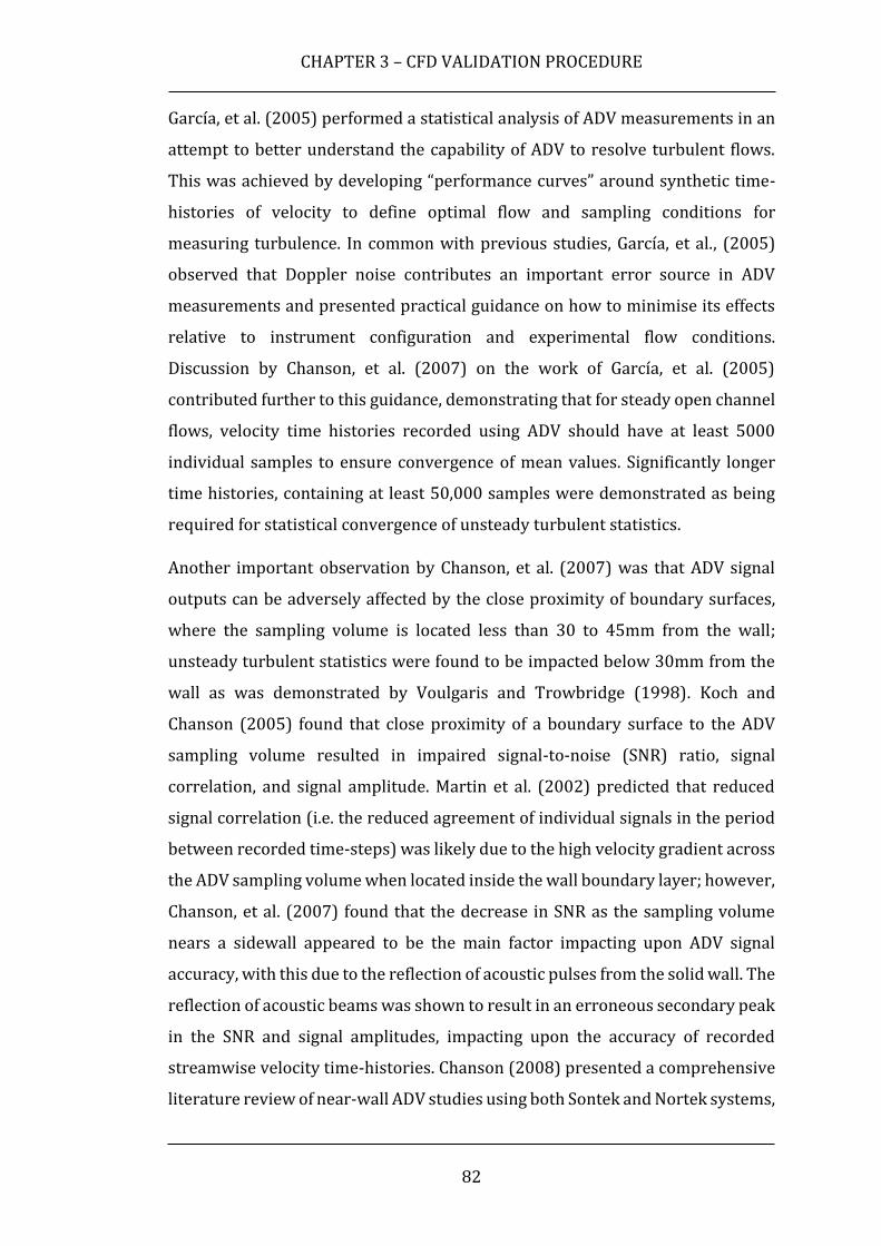
CHAPTER 3 – CFD VALIDATION PROCEDURE
82
García, et al. (2005) performed a statistical analysis of ADV measurements in an
attempt to better understand the capability of ADV to resolve turbulent flows.
This was achieved by developing “performance curves” around synthetic time-
histories of velocity to define optimal flow and sampling conditions for
measuring turbulence. In common with previous studies, García, et al., (2005)
observed that Doppler noise contributes an important error source in ADV
measurements and presented practical guidance on how to minimise its effects
relative to instrument configuration and experimental flow conditions.
Discussion by Chanson, et al. (2007) on the work of García, et al. (2005)
contributed further to this guidance, demonstrating that for steady open channel
flows, velocity time histories recorded using ADV should have at least 5000
individual samples to ensure convergence of mean values. Significantly longer
time histories, containing at least 50,000 samples were demonstrated as being
required for statistical convergence of unsteady turbulent statistics.
Another important observation by Chanson, et al. (2007) was that ADV signal
outputs can be adversely affected by the close proximity of boundary surfaces,
where the sampling volume is located less than 30 to 45mm from the wall;
unsteady turbulent statistics were found to be impacted below 30mm from the
wall as was demonstrated by Voulgaris and Trowbridge (1998). Koch and
Chanson (2005) found that close proximity of a boundary surface to the ADV
sampling volume resulted in impaired signal-to-noise (SNR) ratio, signal
correlation, and signal amplitude. Martin et al. (2002) predicted that reduced
signal correlation (i.e. the reduced agreement of individual signals in the period
between recorded time-steps) was likely due to the high velocity gradient across
the ADV sampling volume when located inside the wall boundary layer; however,
Chanson, et al. (2007) found that the decrease in SNR as the sampling volume
nears a sidewall appeared to be the main factor impacting upon ADV signal
accuracy, with this due to the reflection of acoustic pulses from the solid wall. The
reflection of acoustic beams was shown to result in an erroneous secondary peak
in the SNR and signal amplitudes, impacting upon the accuracy of recorded
streamwise velocity time-histories. Chanson (2008) presented a comprehensive
literature review of near-wall ADV studies using both Sontek and Nortek systems,

CHAPTER 3 – CFD VALIDATION PROCEDURE
83
with the primary conclusion that ADV will tend to under-predict the streamwise
mean velocity component when a solid wall is less than 30 to 45mm from the
ADV sampling volume; this effect was argued by Chanson, et al., (2007) to be
primarily resultant from a reduction in SNR with decreasing distance from the
wall.
More recently, Khorsandi, et al. (2012) performed a comprehensive ADV study,
comparing Flying Hot Film Anemometry (FHFA) measurements around
turbulent jets with those recorded using a Nortek Vectrino ADV system. The
streamwise FHFA measurements were validated against Stationary Hot Wire
Anemometry (SHFA) and LDV data presented by Hussein et al. (1994), while
Khorsandi, et al. (2012) also used the SHFA measurements presented by
Panchapakesan and Lumley (1993) to compare with the vertical velocity
components recorded by a downward-facing ADV. The Vectrino ADV probe was
configured to sample instantaneous velocities at 25Hz and at least 10,000
samples were recorded to ensure statistical convergence; the ADV probe could
also be arranged in either a downward-facing, or spanwise-facing orientation,
allowing the effect of probe orientation upon results to be investigated.
Khorsandi, et al. (2012) initially performed measurements using the downward-
facing ADV probe orientation, which showed increased levels of Doppler noise in
the span-wise and streamwise instantaneous velocity signals, in common with
the findings of Voulgaris and Trowbridge (1998). The presence of noise in the
streamwise velocity component caused an over-estimation of standard deviation
by up to 10%, although the mean velocity in all components were unaffected as
Doppler noise is essentially white noise, and thus has zero mean (García, et al.,
2005). The standard deviation in the vertical component of velocity was found to
be accurate in both standard deviation and mean velocity, again in agreement
with Voulgaris and Trowbridge (1998). Khorsandi, et al. (2012) then re-
orientated the ADV probe with its ultra-sonic signal emitter in the spanwise
direction, before performing further measurements. This time, it was observed
that high levels of Doppler noise were present in the streamwise and vertical
velocity components, while the spanwise component (i.e. the velocity component
aligned with the ultra-sonic signal emitter) showed good agreement for standard

CHAPTER 3 – CFD VALIDATION PROCEDURE
84
deviation. Again, accurate mean velocities were recorded for all velocity
components. This showed that while accurate mean velocities will be recorded
in three-components, only the component aligned with the ultrasonic signal
emitter will yield reliable unsteady turbulent statistics, due to the presence of
Doppler noise in the other two components.
In addition to the presence of random Doppler noise in the two velocity
components not aligned with the ADV signal emitter, additional sampling errors
will inevitably intrude into all three flow components through a variety of
mechanisms. Indeed, it is known that a combination of sampling errors,
installation vibrations, and Doppler noise can change the character of measured
turbulence considerably (McLelland & Nicholas, 2000) (Nikora & Goring, 1998).
As a result, a good understanding of proper ADV experimental set-up is necessary
to minimise noise during data recording, while post-processing must be
employed to eliminate spurious data samples where possible. The critical
importance of this post-processing of ADV data was shown conclusively by
Chanson et al. (2008), who used ADV in a small estuary, concluding “turbulent
properties cannot be derived from unprocessed ADV signals”. Some of the more
commonly used methods of detecting erroneous data were outlined by Wahl
(2000), before describing the WinADV program, a publicly-available signal
filtering tool developed for use with ADV, and designed to intelligently filter
unwanted sources of noise during post-processing of results. This filtering is
performed using a range of techniques, including an adaption of the “spike
detection” filter discussed by Wahl (2003) and first proposed by Goring and
Nikora (2002) at the New Zealand Institute for Water and Atmospheric Research
(NIWA). In experimental studies, any unfiltered ADV data is generally not
recommended for analyses. Given the susceptibility of ADV to signal noise, the
WinADV program, written in Visual Basic and compiled for use with a standard
Windows computer, is now widely used for post-processing of output ADV data.
Khorsandi et al. (2012) used WinADV in an effort to remove noise from ADV data
with some success, with ADV standard deviations reduced to levels closer to
those recorded using FHFA, however standard deviations were found to still be

CHAPTER 3 – CFD VALIDATION PROCEDURE
85
higher in signals containing Doppler noise, in comparison with signals recorded
using other experimental approaches.
Experience during recent studies using ADV at UoL were consistent with the
literature, with ADV shown to offer a reliable method of measuring three-
component mean velocities in a given sampling volume, and providing reliable
unsteady turbulence measurement in one direction aligned with the ADV
ultrasonic emitter. At Liverpool in 2014, Tedds found that for ADV measurement,
“Different probe orientations [measuring at the same point] give the same mean
but different Reynolds normal stresses”, before concluding that, “ADVs are good
at showing trends in the flow and provide a good qualitative data set to compare
general flow characteristics.” (Tedds, 2014)
Further studies by Henriques, et al. (2014) in the recirculating water channel at
Liverpool have confirmed these findings, with ADV demonstrated to be a useful
method for determining the mean and RMS flow for a given fluid volume,
provided its limitations are well understood. For this reason, ADV was used for
measuring the mean velocities in addition to unsteady turbulent statistics at
various locations around the model QEC, to provide a quantifiable measure of
accuracy for the CFD airwakes.
3.2.3.2 ADV Experimental Procedure
For this study, a Nortek Vectrino+ ADV system was used complete with two
measurement probes, as shown earlier in Fig 48. The first probe is a downward-
looking probe attached to the Vectrino+ unit via a one metre flexible cable,
allowing unsteady velocity to be measured in the vertical (z) flow direction at
maximum depth in the water channel, while the second probe is side-looking -
also on a one metre cable - allowing the span-wise (y) unsteady velocity
component of the flow to be measured.
As previously discussed, the Nortek Vectrino+ can measure the three velocity
components at up to 200Hz, however it will yield useful unsteady statistics only
in the direction of the acoustic transmit transducer. While the other two velocity
components can be used to give a reliable mean velocity (typically within 1%),

CHAPTER 3 – CFD VALIDATION PROCEDURE
86
they cannot be used to determine instantaneous velocity due to increased levels
of signal noise present in the two velocity components normal to the transmit
transducer. To illustrate this point, Fig 49 shows a time history recorded using
the Vectrino+ ADV down-looking probe. The time history was recorded in the
centre of the water channel with undisturbed flow, running at a 1m/s flow speed.
The water channel has been calibrated in a previous study using LDV (Tedds,
2014). The flow was sampled at 200Hz for a period of 50 seconds, yielding 10,000
total samples as advised by Chanson, et al. (2007) for the determination of usable
flow statistics.
As can be seen in Fig 49, the mean velocities are close to expected values, with
the u-component and w-component being outside expected values by 3% and -
2%, respectively. The mean velocity for the v-component can be seen to be at
exactly the expected value of 0.0m/s; this is because rotation of the Vectrino+
probe about its vertical axis, and thus adjustment of the v-component, is capable
of the most precise adjustment in the experimental arrangement, as outlined
later in this chapter. For the u- and w-components however, precise alignment is
more difficult, and therefore it is anticipated that the minor discrepancy in w-
component velocity is due to the probe not being positioned in a perfectly vertical
orientation, causing some of the stream-wise velocity to be experienced as w-
component (vertical) velocity. Using trigonometry, the ADV transmitter was
estimated to be slightly out of alignment by -1.18° in the pitch degree of freedom,
with the net velocity magnitude virtually unchanged from the u-component
velocity at 0.971m/s. The ADV probe can be seen to yield a reliable mean in three
velocity components in its own “local” coordinate frame; however, the accurate
orientation of the probe is critical to ensure the local coordinate frame of the ADV
probe aligns with the “global” coordinate system of the water channel, to enable
a meaningful comparison between the individual velocity components of
experimental and computational results. The accurate positioning of the ADV
probes in six degrees of freedom was given consideration during the design of
the traverse system, discussed later in this chapter.
The effect of Doppler signal noise, discussed above, upon ADV velocity
components measured using a down-facing probe can be immediately seen in Fig

CHAPTER 3 – CFD VALIDATION PROCEDURE
87
49. Measured in uniform flow, signal noise can be seen to be present in the two
velocity components normal to the acoustic transmitter – u and v – while the
velocity component orientated with the transmitter can be seen to have
markedly reduced levels of noise present in the recorded velocity time history.
Fig 50 shows histograms of these three velocity components recorded by the
down-facing probe. The three components are shown as frequency distributions,
with the u-component and v-component similar in their sample deviations from
their respective means, having 95% of instantaneous velocity samples occurring
within a range of 0.16m/s (i.e. ±2σ). The w-component velocity however, occurs
over a much narrower velocity range as expected for steady flow conditions, with
95% of samples occurring within a range of 0.04m/s (±2σ).
Changing the down-looking probe for a side-looking probe will allow accurate
unsteady turbulence statistics to instead be measured along the v-component of
velocity, as shown in Fig 51. With the side-looking probe now fitted, the mean
velocities are comparable to those measured previously using the down-facing
probe. Reduced levels of signal noise are now present in the v-component of
velocity, at the expense of increase noise in the w-component. Due to the inherent
design of ADV, low noise streamwise u-component velocity can never be
captured however, resulting in diminished accuracy of three-dimensional RMS
measured using ADV, with over-prediction occurring due to over-estimation of
unsteadiness in the streamwise component from signal noise. As can be seen in
Fig 52, the v-component of velocity now has a much reduced velocity range,
having a range of 0.04m/s (±2σ).
Another important consideration when designing an experimental study using
ADV is spatial accuracy. ADV measures velocity within a small volume rather than
at a single point, and so there will inevitably be some uncertainty when
performing comparison with CFD measured at a single point. The ADV probe
used in this study was configured to measure a cylindrical domain, having a 7mm
diameter, and height 15mm. The ADV transducer is positioned 50mm from the
centroid of this measurement volume, further complicating the accurate
positioning of the probe.

CHAPTER 3 – CFD VALIDATION PROCEDURE
88
Fig 49: Time History of Velocity Components Measured with Down-Looking Probe
Fig 50: Histogram of Down-Looking Probe Velocity Components

CHAPTER 3 – CFD VALIDATION PROCEDURE
89
Fig 51: Time History of Velocity Components Measured with Side-Looking Probe
Fig 52: Histogram of Side-Looking Probe Velocity Components

CHAPTER 3 – CFD VALIDATION PROCEDURE
90
When performing measurements around a scale model, minor variation in the
exact measurement point at model scale can correspond to significant spatial
variation at full-scale. For the QEC 1:202 scale model ADV measurements, a
spatial variation of ±7.5mm at model scale (i.e. the height of the measurement
volume) will equate to a ±1.515m variation at full scale. While not a significant
variation across the length of a 280m aircraft carrier, when measuring the wake
of smaller features with correspondingly smaller turbulent length scales, this
spatial variation becomes more significant. For example, when performing a
comparison between ADV and CFD at a point in the lee of the QEC forward island,
where complex vortex shedding results in flow reversal, such spatial variation in
measured points can potentially impact significantly upon the agreement of the
results. It is therefore important to design an ADV experiment to ensure accurate
positioning of the probe in the water channel, with a procedure in place to
determine the exact location of the ADV measurement volume centroid relative
to the ship. This positioning will minimise systematic errors in the measurements
around the model. Consideration was given to the accurate positioning of the
ADV measurement volume centroid, during the calibration of the probe.
The advantages of using ADV for experimental validation of CFD simulations have
been outlined in this section. ADV can yield accurate three-dimensional
components of mean velocity inside a known measurement volume, in addition
to providing accurate unsteady statistics for two velocity components, by
performing two measurements at a point (with a down-facing, then side-facing
probe). However, the limitations of ADV should be understood during the
experimental design phase to ensure reliability of measurement. ADV is an
excellent tool in the pursuit of CFD validation, as the two approaches are mutually
complementary. ADV allows validation of unsteady CFD computations at high
frequency, while the newly-validated CFD computations can then be used to gain
a better understanding of the unsteady flow in the region of interest.
3.2.4 ADV Traverse System
In previous studies at UoL, the Vectrino ADV unit was positioned in the water
tunnel using a steel cross-beam fixed across the top of the working section. This
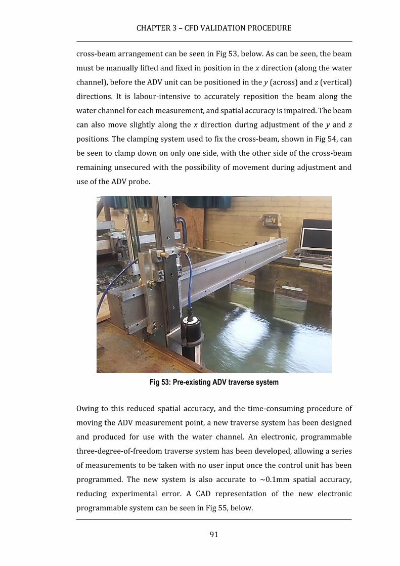
CHAPTER 3 – CFD VALIDATION PROCEDURE
91
cross-beam arrangement can be seen in Fig 53, below. As can be seen, the beam
must be manually lifted and fixed in position in the x direction (along the water
channel), before the ADV unit can be positioned in the y (across) and z (vertical)
directions. It is labour-intensive to accurately reposition the beam along the
water channel for each measurement, and spatial accuracy is impaired. The beam
can also move slightly along the x direction during adjustment of the y and z
positions. The clamping system used to fix the cross-beam, shown in Fig 54, can
be seen to clamp down on only one side, with the other side of the cross-beam
remaining unsecured with the possibility of movement during adjustment and
use of the ADV probe.
Fig 53: Pre-existing ADV traverse system
Owing to this reduced spatial accuracy, and the time-consuming procedure of
moving the ADV measurement point, a new traverse system has been designed
and produced for use with the water channel. An electronic, programmable
three-degree-of-freedom traverse system has been developed, allowing a series
of measurements to be taken with no user input once the control unit has been
programmed. The new system is also accurate to ~0.1mm spatial accuracy,
reducing experimental error. A CAD representation of the new electronic
programmable system can be seen in Fig 55, below.

CHAPTER 3 – CFD VALIDATION PROCEDURE
92
Fig 54: Pre-existing ADV traverse attachment clamp (left), and free-standing foot (right)
Fig 55: CAD model of a 3DOF fully programmable traverse system
The traverse system is comprised of two traverses along the length of the water
channel, with one configured as a “master” (driven by a stepper motor), and the
second “slave” unit driven by a driveshaft connected to the master unit. A third
traverse is fitted across the water channel, supported by a simple slide-rail. The
slide-rail is required due to the susceptibility to torsion of the Y-axis traverse
unit. The system is driven by three stepper motors (one per degree of freedom),
which are in turn driven by three stepper cards mounted to a control unit. User
inputs are then made via a Windows computer, connected to the control unit
using a USB cable.
As outlined previously, the orientation of the ADV probe relative to the water
channel flow is important for the accurate representation of the three measured

CHAPTER 3 – CFD VALIDATION PROCEDURE
93
velocity components, and so consideration was given to ensure accurate
positioning of the traverse system relative to the fluid flow. The traverse system
was attached using dowels to four one-inch thick locating pads, with one pad
fitted to each corner of the system. Laser alignment was used to ensure accurate
location of the traverse in the u-component (streamwise), before the pads were
carefully machined to ensure the traverse ran parallel to the water surface,
ensuring alignment in the w-component (upwards). The locating dowels were
located using a clearance fit, allowing the traverse system to be easily removed if
required for future experimental studies, and later accurately refitted relative to
the fluid flow.
3.2.5 Experimental Validation Results
Once the Nortek Vectrino+ ADV probes and three-dimensional electronic
traverse systems were successfully integrated with the recirculating water
channel, measurements were performed across the QEC experimental model for
the purposes of comparison with CFD results to gain an understanding of the
accuracy of the generated airwakes; the results of this comparison are discussed
in this section.
Comparisons between QEC CFD and water channel experiment have shown
overall favourable results, with the character of the ship’s airwake well captured
by the simulated airwakes. However, it should be noted there are expected to be
some minor differences between the full-scale ship CFD and the model-scale
water channel experimental model. The main differences between experiment
and CFD are the differing inlet velocities and boundary conditions, and the lack
of Reynolds number matching between experiment and full-scale QEC. Each of
these points are outlined as follows:
As outlined in Chapter 2, the full-scale QEC CFD features a velocity profile
at the inlet representative of an oceanic ABL, while the water channel
working section has a largely uniform velocity inlet. This has been
corrected for in the data presented in this section by normalising mean
velocity data in the CFD results by the freestream anemometer velocity

CHAPTER 3 – CFD VALIDATION PROCEDURE
94
value. This has proven to be generally effective in providing a comparison
between model-scale and full-scale, however the impact of this variation
in velocity cannot be properly understood without computing additional
CFD of the water channel working section at the model-scale. The
computation of model-scale CFD was recommended to better understand
the subtle differences between model-scale and full-scale.
Differing boundary conditions between full-scale and model-scale are
inevitable, due to the size limitations of the recirculating water channel
working section. While the full-scale ship CFD was intended to represent
oceanic conditions, and so lack any no-slip walls in the computational
domain, the water channel is bounded by no-slip walls and floor, in
addition to the free surface 0.84m above the QEC experimental model. The
effects of differing boundary conditions upon the solution were
considered earlier in this chapter, with the experimental model scale
carefully designed to limit the maximum fluid acceleration due to
blockage at 3.3%.
The difference in Reynolds number between full-scale CFD and model-
scale experiment is an inevitable result of the very large size of an aircraft
carrier compared with the comparatively small size of its corresponding
experimental model, as discussed earlier in this chapter. Despite the
positive impact of using water instead of air at the model-scale (Re~106),
Reynolds number was not matched to full-scale (Re~108). Although
previous studies have demonstrated aircraft carrier airwake to be
Reynolds number independent (Polsky & Bruner, 2000), the exact effect
upon the airwake at model-scale are not fully understood and further
investigation is recommended.
Given the above differences between full-scale CFD and model-scale experiment
of the QEC, generally good agreement has been found, demonstrating that the
QEC CFD is a suitable representation of airwake passing over the ship in oceanic
conditions. Examples of this validation are presented in the remainder of this
chapter.

CHAPTER 3 – CFD VALIDATION PROCEDURE
95
3.2.5.1 SRVL Glideslope
The SRVL glideslope is an important area of the QEC airwake when used for fixed-
wing piloted flight simulation; it is also the most difficult to accurately capture
using CFD, due to the potential for non-physical numerical dissipation which can
occur, as outlined in Chapter 2. The CFD computations along the SRVL flight path,
which follows a 7° glideslope on approach to the touchdown point, must be
reliable at up to 400m (~1.5 ship lengths) behind the stern of the ship to ensure
a realistic experience for the test pilots, and so turbulence must be preserved in
the CFD solution up to this distance.
An experimental run was performed using the ADV probe along the 7° SRVL
approach path, downstream of the QEC model. A total of 103 individual test
points were measured by the probe along the SRVL glideslope, with a spatial
increment of 2.5cm in x along the ship centre-line. The ADV probe was
programmed to sample at 200Hz for 60 seconds at each measurement point,
yielding 12,000 data samples per point to ensure convergence of turbulent
statistics. The accuracy in the measurement of the mean flow velocity
components is quoted by the ADV manufacturer to be ±0.5%; experience with
the probe suggests there is an additional uncertainty due to the size of the
measurement volume and so an estimate of the experimental uncertainty in the
probe is ±1% (Tedds, 2014).
An initial comparison was made between CFD and the ADV experiment results
along the SRVL 7° centre-line; this comparison can be seen in Fig 56. It should be
noted that due to the presence of the ABL profile obtained from Eqn (5) in the
CFD data, which results in varying u-component velocity with height above sea
level, unlike the uniform inlet velocity profile in the experiment, it was necessary
to normalise each CFD data-point by ABL streamwise velocity at each height
above sea level. The normalisation of CFD velocity components by height allowed
an initial comparison to be made between full-scale CFD and water-tunnel
experimental data.
As can be seen from Fig 56, the mean u-component velocity (WOD) offers
reasonably good agreement between ADV and CFD along the SRVL glideslope
immediately aft of the ship, with the peak velocity and its position accurately

CHAPTER 3 – CFD VALIDATION PROCEDURE
96
captured at approximately half a ship’s length from the carrier pitch-centre. At
two ship lengths from ship pitch centre, a slight ADV velocity peak can be seen,
which is thought to be from the free-surface effects present in the water channel
at this height. Very near to the ship, it can be seen that ADV and CFD data diverge;
this could be due to differences in surface roughness between CFD and the
experimental model, and possible interference between the model surface and
ADV sampling volume. Further investigation is necessary to determine the cause
of this behaviour. The w-component velocity (upwash) in Fig 56 again shows
good agreement in terms of position of the peak downwash, however the
magnitudes of ADV data differs consistently across the SRVL glideslope; this may
be caused by the ADV probe being orientated slightly off-vertical, resulting in a
slight interference from u-component velocities in the smaller w-component
velocities. The v-component velocities (cross-wind, negative to starboard) in Fig
56 are very small but nevertheless can be seen to show good agreement along
the SRVL glideslope between ADV and CFD. In particular, turbulent effects caused
by the aft island can be seen to be captured in both experimental and
computational results for the v-component velocity.

CHAPTER 3 – CFD VALIDATION PROCEDURE
97
Fig 56: Comparison between CFD and experimental data along QEC SRVL glideslope;
u-, v-, and w-components

CHAPTER 3 – CFD VALIDATION PROCEDURE
98
3.2.6 Expanding the Project
At this point in the research it became apparent that the priority for the wider
project was to provide CFD-generated airwakes to BAE Systems for
implementation into their flight simulator so that simulated flight trials could be
conducted by F35-B test pilots, and for the UoL helicopter/QEC flight simulation
environment to be developed and implemented. A second industrial CASE PhD
project was therefore established in collaboration with BAE Systems to conduct
a greater in-depth study of the flow in the water channel and at different angles
of orientation of the QEC model. The author of this thesis has therefore worked
closely with the new PhD student, Neale Watson, to hand over knowledge of the
experimental procedure, and of the CFD process that would need to be adapted
to compute the flow over the QEC model in the water channel. This second project
is now well underway and the results will be reported in detail in future co-
authored publications. However, to provide further evidence to support the CFD
methodology developed in this thesis, the following figures show a selection of
data that has been jointly obtained in the Ahead flow condition.
A comparison is shown in Fig 57 of the mean streamwise velocities along vertical
lines at various positions over and astern of the ship, in a plane through the
centre of the islands. The CFD was computed for the model ship in the water
channel and is shown as continuous lines. The experimental measurements are
shown as black dots and the agreement with the CFD can be seen to be excellent.
The airwake is illustrated by contours of turbulence intensity, defined as the root
mean square of the velocity component divided by the freestream flow velocity.
The computed and measured vertical velocities along the 7° SRVL flight path are
shown in Fig 58. The agreement between CFD and experiment is again seen to
be excellent, and the downward velocity in the lee of the ship’s stern, referred to
earlier, can be clearly seen.
Finally, Fig 59 shows a comparison between the full-scale CFD and the CFD of the
model-scale ship in the water channel. Considering that the water channel has a
uniform inlet velocity profile and the full-scale has an ABL, and the differences in
Reynolds number, the agreement is very good. It also implies that the CFD
methodology is best validated by direct comparison between the model-scale

CHAPTER 3 – CFD VALIDATION PROCEDURE
99
CFD and experiment rather than by comparing the model-scale experiment with
the full-scale CFD.
As intimated above, this model-scale study is ongoing and data showing further
good agreement between the other velocity components and turbulence
intensities will be published in due course, as will similar data for the model ship
in oblique and beam orientations.
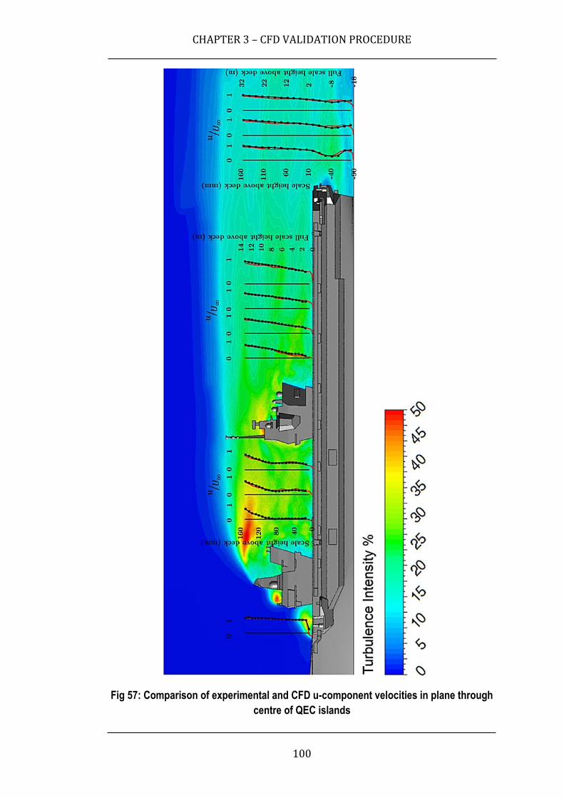
CHAPTER 3 – CFD VALIDATION PROCEDURE
100
Fig 57: Comparison of experimental and CFD u-component velocities in plane through
centre of QEC islands

CHAPTER 3 – CFD VALIDATION PROCEDURE
101
Fig 58: Comparison of CFD and experiment mean w-velocities along 7° SRVL
glideslope

CHAPTER 3 – CFD VALIDATION PROCEDURE
102
Fig 59: Comparison of small-scale and full-scale CFD results in u-velocity component

CHAPTER 3 – CFD VALIDATION PROCEDURE
103
3.3 Chapter Summary
The validation process followed for the generated QEC CFD airwakes has been
outlined in this chapter, the first part of which presented a comparison between
a CFD airwake model of the flow around a US Navy helicopter carrier (USS Peleliu,
LHA-5) with full-scale ultrasonic anemometer measurements recorded at sea.
The second part of this chapter outlined the design and use of a novel purpose-
designed water channel experiment using the ADV measurement technique to
perform measurements around a 1:202 scale model of a QEC aircraft carrier.
Overall, favourable agreement was observed between LHA CFD and ultrasonic
anemometer data, with the w-component of flow shown to have particularly good
agreement. The u- and v-components of the flow were also shown to agree at the
majority of the data-points, with dominant flow features such as the channelling
of flow around the ship’s island observed in both CFD and experimental data.
However, some of the experimental points were found to disagree in azimuth
with points around them in a non-physical way, indicating measurement errors
occurred at these points. This non-physical behaviour was considered to be likely
due to the highly changeable conditions inevitably encountered at sea during
testing, with freestream atmospheric conditions varying considerably in the time
required to recorded data at 44 sample points, having a finite number of
ultrasonic anemometers available during the trial.
As a result of these findings, it was concluded that while full-scale anemometer
data from sea trials can be used satisfactorily to observe general flow behaviour
across the deck, the highly changeable freestream conditions at sea will limit the
ability of recorded data to capture smaller variations in flow around the ship, as
these features are likely to be masked by variations in flow due to atmospheric
conditions. Further, as no experimental data was available for LHA along the
SRVL glideslope behind the ship, it was not possible to adequately demonstrate
the important requirement of preservation of turbulence up to 0.25 miles aft of
the ship. To ensure accurate capture of flow features characteristic of the QEC,
and to ensure numerical dissipation is minimised along the ship’s SRVL
glideslope, a further experimental study was therefore required, using a facility
where the inlet conditions can be more precisely controlled. As a result, a further

CHAPTER 3 – CFD VALIDATION PROCEDURE
104
validation experiment was designed and built using the large recirculating water
channel at UoL, where freestream conditions can be precisely controlled to
enable higher resolution of validation of flow features to be carried out across
the QEC. The design and implementation of this water channel experiment was
described in the second part of this chapter.
Once built, the water channel experiment was used to perform a study along the
F-35B’s SRVL glideslope up to 0.25 miles aft of the ship, to demonstrate
numerical dissipation of turbulence in the CFD solution has been minimised. The
initial outcome of this investigation demonstrated good agreement between CFD
and experiment along the SRVL glideslope, giving confidence that the CFD
airwakes generated are suitable for use in piloted flight simulation.
However, whilst encouraging agreement was demonstrated for mean velocities
between experimental ADV and computational CFD results, it became evident
that an additional project, focussed on the water channel experiments, was
required. This new project was established during the course of the research
described in this thesis, and with input from the thesis author. Initial joint results
between the two projects have therefore been presented in this chapter and give
even greater confidence that the CFD technique is producing verifiable QEC
airwakes.
Having created a number of full-scale CFD airwakes for the QEC at different wind
conditions (a process that is ongoing at the time of writing), the next challenge
was to integrate these into flight simulation facilities, which will be described in
the next chapter.

CHAPTER 4 – FLIGHT SIMULATOR INTEGRATION
105
Chapter 4 – Flight Simulator Integration
Having generated the full-scale CFD airwakes and having conducted experiments
to give confidence in their accuracy, the next work package on the flow diagram
given in Fig 11 was to integrate these large QEC airwakes into the flight
simulators at UoL and BAE Systems Warton. It was important that the airwake
data files delivered to BAE were correctly formatted and documented for
integration into the F35-B simulator; the integration and implementation of the
airwakes was conducted by BAE flight simulation engineers. The process of
integrating the airwakes into the HELIFLIGHT-R simulator is outlined in this
chapter, beginning with a description of the flight simulation facilities at UoL. The
procedure for converting the unstructured CFD data into a format useable by the
flight simulators is outlined, along with a brief description of the mathematical
aircraft model used for the simulation trial.
4.1 HELIFLIGHT-R Flight Simulator
The QEC helicopter flight trial was performed in the HELIFLIGHT-R
reconfigurable piloted flight simulator; one of two motion-base flight simulators
at UoL. The development of the original single-seat motion-base flight simulator,
HELIFLIGHT, was described by Padfield and White (2003). The newer, more
capable HELIFLIGHT-R simulator consists of a fully reconfigurable crew station
which, for the purposes of this trial, was arranged as a generic two pilot rotorcraft
cockpit plus a third instructor seat in the rear. Views of outside and inside
HELIFLIGHT-R can be seen in Fig 60, with the QEC visual environment shown
(White, et al., 2012). The crew station is housed within a 12-foot diameter
carbon-fibre dome, onto the inside of which three high resolution Liquid Crystal
on Silicon (LCoS) projectors provide a 220x70° field of view. The advantage of

CHAPTER 4 – FLIGHT SIMULATOR INTEGRATION
106
LCoS is that it does not present symptoms of “pixel-gridding”, as seen in LCD.
Edge-blending and geometry correction is carried out using a Rockwell Collins
Mercator pixel management system to ensure one uniform image is shown to the
pilot across the inside surface of the dome. Two 19” LCD monitors are used to
increase the pilot’s field of view to include views through the helicopter chin
windows, in addition to a further two 19” LCD monitors mounted inside the
cockpit, on which aircraft instrumentation is displayed to the pilot using Presagis
VAPS XT software. Visuals are generated using Vega Prime visualisation
software, complete with the Vega Prime Marine add-on to yield realistic dynamic
ocean surfaces for offshore simulation. This visual model is then integrated into
the simulator run-time environment, LIVE (White, et al., 2017).
Fig 60: HELIFLIGHT-R piloted flight simulator (left foreground) with QEC visual
environment
The HELIFLIGHT-R platform is capable of six Degrees of Freedom motion,
employing six actuators each with a 24-inch stroke. The maximum Gross Moving
Payload of the motion base is rated at 1800kg, while the cockpit in its current
configuration is estimated at 900kg. The rated performance envelope for the
HELIFLIGHT-R motion base is given in Table 1. Motion base acceleration

CHAPTER 4 – FLIGHT SIMULATOR INTEGRATION
107
commands are provided as outputs from the aircraft model and are passed
through a motion drive algorithm as described by Hodge (2010). A fully
programmable control loading system provides force-feedback through the
aircraft cyclic, collective, and pedal inceptors to provide a more realistic
experience to the pilot and co-pilot and is driven by the aircraft mathematical
model.
Table 1: HELIFLIGHT-R rated performance envelope (White, et al., 2012)
Integration of the mathematical aircraft model with the simulator is undertaken
by Advanced Rotorcraft Technology’s (ART’s) FLIGHTLAB software (Du Val,
2016), which provides a library of aircraft models including a Generic Rotorcraft
Model, similar to a Sikorsky UH-60A Blackhawk, which was reconfigured to be
representative of a SH-60B Seahawk for the piloted flight trial to be described in
Chapter 5. CFD airwakes can be loaded into FLIGHTLAB as lookup tables of time-
varying three-dimensional velocity components, enabling unsteady aerodynamic
loads to be imposed upon the aircraft flight model. During testing, FLIGHTLAB
allows real-time data monitoring and recording which, together with in-cockpit
additional video and audio files, are used for post-trial analysis.
4.2 Aircraft Model
The flight trial was conducted using FLIGHTLAB’s generic helicopter model
configured to be representative of a Sikorsky SH-60B Seahawk, which is a four-
bladed twin-engine multi-mission maritime helicopter; a schematic diagram of
this aircraft is shown in Fig 61 complete with general dimensions. The SH-60B

CHAPTER 4 – FLIGHT SIMULATOR INTEGRATION
108
aircraft mathematical model was selected for use in the trial as it is based on the
Generic Rotorcraft Model that has been extensively validated, under a
Cooperative Research and Development Agreement (CRADA) with the US Army’s
Aero Flight Dynamics Directorate (AFDD). Although the SH-60B Seahawk is not
in use with the Royal Navy, it was decided that this aircraft would be used for the
proof-of-concept QEC simulated flight trial due to its strong validation and
previous use at Liverpool (Kääriä, et al., 2009).
The FLIGHTLAB model of the SH-60B comprises the following major subsystem
components: (1) individual blade-element main-rotor model including look-up
tables of non-linear lift, drag and pitching moment coefficients stored as
functions of incidence and Mach number; (2) Bailey disk tail-rotor model, (3)
finite-state Peters-He dynamic inflow model; (4) separate look-up tables for the
fuselage, vertical tail and the port and starboard stabilator forces and moments
stored as nonlinear functions of incidence and sideslip; (5) turbo-shaft engine
model with a rotor-speed governor; (6) primary mechanical flight control system
and stability augmentation system models including sensor and actuator
dynamics; and (7) a landing gear model to provide deck reactions cues on
touchdown. Padfield (1996) describes this level of modelling as medium fidelity,
capable of simulating trim and primary-axis responses faithfully. Handling
qualities characteristics are also generally well predicted using this type of flight
dynamics model.

CHAPTER 4 – FLIGHT SIMULATOR INTEGRATION
109
Fig 61: Schematic views and dimensions of a Sikorsky SH-60B Seahawk (Hodge, 2010)
4.3 WOD Conditions
The purpose of this initial simulated flight trial was to demonstrate capability of
the QEC dynamic interface simulation, and so it was deemed that for this
exploratory study landings would be performed for three wind-speeds (25kt,
35kt, and 45kt), at two WOD conditions – Ahead, and Green 25° (i.e. from
starboard). This would permit the flight trial to focus upon achieving

CHAPTER 4 – FLIGHT SIMULATOR INTEGRATION
110
demonstrable results for a selection of conditions without attempting a full
simulated FOCFT for the SH-60B to QEC. Computed CFD solutions for Ahead and
Green 25° at 35kt were used for the trial.
Previous studies by Polsky and Bruner (2000), and Forrest (2009) demonstrated
that ship airwakes can be computed at one wind speed and scaled to accurately
represent a higher or lower wind speed. The vortices shed from bluff bodies
within a flow are created at distinct frequencies which can be described by the
Strouhal Number (Reynolds number dependence is acknowledged but is known
to be less important at high values and for sharp-edged bodies). Strouhal number,
Eqn (13), relates the characteristic length of a bluff body, L, the flow speed, V, and
the frequency, f, of the vortices shed from the body. This simple relationship
shows that for an increase in free stream speed there will be a proportional
increase in shedding frequency, and for an increase in length scale there will be
a proportional decrease in frequency. While this may be obvious for vortex
shedding at a single frequency from a bluff body with a single characteristic
length, the principle can also be extended to more complex shedding from the
multiple bluff bodies that make up a ship’s superstructure. As a result, for each
wind heading a single wind speed can be computed and then any desired wind
speed can be quickly created by post-processing without the need to run further
expensive CFD solutions. The ability to generate airwake at one wind speed for
each azimuth in this way is advantageous as it greatly reduces the number of CFD
runs that must be completed to simulate a full WOD envelope for a ship.
𝑆𝑡 =𝑓𝐿
𝑉 (13)
Therefore, one wind speed (35kt) was computed for each wind azimuth, with
each computed airwake then scaled by a multiplication factor where a different
wind speed is desired. For example, where the 35kt airwake data was scaled to
represent a 45kt condition, the time-step size and velocity components were
multiplied by a factor of 9⁄7, having the effect of scaling both the velocity
magnitudes and frequencies of the airwake to the desired 45kt condition.

CHAPTER 4 – FLIGHT SIMULATOR INTEGRATION
111
The file-size of airwake data required for the CFD simulations was found to be a
challenge during the development of the QEC DI simulation, much more so than
previous experience with smaller frigates. Unstructured airwake data files
(containing full simulation data) were approximately 3.5TB per wind-direction.
Manipulation of this data presented challenges and could not be economically
performed using desktop computers. Instead, HPC was used for some data
processing, placing increased demands upon shared resources. Data storage and
transfer also presented challenges, where even the fastest Solid-State Drives
(SSD) reading/writing at 550/520MB/s require approximately two hours to read
a full set of airwake data.
Upon completion of a CFD simulation for a given wind azimuth, the airwake
velocity data was then converted into a format which could be integrated into the
HELIFLIGHT-R flight simulator. The unstructured CFD data was first interpolated
onto a structured grid in the region of interest, before being output in an ASCII
text format. An example structured grid can be seen in the lower-left of Fig 62.
Once converted into a structured format, the output ASCII airwake data can then
be imported into a new Simulink airwake module that interfaces with the
simulator’s flight mechanics modelling software. Verification takes place to
ensure that the airwake is correctly positioned relative to the ship’s visual model
in the flight simulator environment, with this verification procedure outlined
later in this chapter. Upon completion of verification checks, the SH-60B can be
‘flown’ in the airwake, with the SH-60B mathematical model integrating the
effects of the airwake at various Aerodynamic Computation Points (ACPs) on the
helicopter. The positions of the ACPs on the SH-60B model can be seen as red
points in the upper-right of Fig 62, with ten ACPs on each of the four main rotor
blades, one ACP at the fuselage (ACP3), one ACP on each of the port and starboard
stabilisers, two ACPs on the vertical tail, and a final ACP at the centre of the tail
rotor hub, to give a total of 46 ACPs.

CHAPTER 4 – FLIGHT SIMULATOR INTEGRATION
112
Fig 62: Conversion process for unstructured data into a format readable by the ACPs
on the SH-60B aircraft model
4.4 CFD Interpolation Sizing
The sizing of the CFD airwake was limited by the amount of Synchronous
Dynamic Random-Access Memory (SDRAM) available to the flight simulation
computer responsible for integration of transient airwake into the LIVE
simulation environment. For HELIFLIGHT-R, this limit is 32GB DDR4 SDRAM. In
terms of airwake size, this was found to equate to approximately 1 billion
individual velocity samples, resulting in a maximum interpolation box volume of
approximately 1 million cubic metres for a recorded time history of 30 seconds
at 25Hz. In contrast, the F-35B flight simulation facility at BAE Systems Warton
is capable of an interpolation volume size of 10.08 million metres cubed at the
same recorded time and frequency, due to the increased SDRAM available at that
facility (1TB). A comparison of the BAE and UoL interpolation box sizes is shown
in Fig 63, plus comparison with previous interpolation box sizes used for
simulated deck landings to frigates and destroyers at UoL. As can be seen, the size
of the data recorded, converted, and imported into HELIFLIGHT-R for QEC is
several orders of magnitude greater than previous projects at UoL.

CHAPTER 4 – FLIGHT SIMULATOR INTEGRATION
113
Fig 63: Interpolation box sizing for UoL and BAE simulators, compared with previous
interpolation box sizing used for frigates and destroyers at UoL
Also shown in Fig 63, are the expected SRVL and VL approaches for fixed-wing
and rotary-wing aircraft to QEC, with the complete operation of both SRVL and
VL captured by the BAE interpolation grid. The coordinates for QEC interpolation
boxes are given in Table 2, in addition to interpolation sizing for a typical frigate
or destroyer using HELIFLIGHT-R. The UoL interpolation grid can be seen to
capture VL operations well, but does not encompass all of the SRVL approach, in
particular the tip-over point. For this reason, while the HELIFLIGHT-R is only
intended for simulation of VL operations to QEC, it is recommended that for any
future work involving SRVL simulation a new interpolation box for SRVL is
developed which neglects VL operation from the port side of the ship to better
incorporate the narrow glideslope on approach to the ship. A proposed
interpolation box suitable for SRVL testing in HELIFLIGHT-R, is also included in
Table 2, with the proposed dimensions containing the same number of airwake
sampling points as for the VL interpolation box, while still encompassing the
SRVL glideslope.

CHAPTER 4 – FLIGHT SIMULATOR INTEGRATION
114
Table 2: QEC interpolation box coordinates, relative to ship CG at sea-level
4.5 HELIFLIGHT-R airwake checks
Once loaded into the LIVE interface, the airwake files were checked to ensure
they were correctly located in the simulation environment. Coordinate points
were checked at three positions in the CFD mesh and compared with coordinate
points of the same positions in the QEC visual model to ensure correct alignment
of the airwakes with the visual environment. Once aligned, time histories of
airwake velocity recorded during the original computation of the CFD were
compared at the three points in the domain with measurements of airwake
recorded at the same points read by the aircraft flight model and output from the
flight simulator. The locations of the three comparison points (A, D, and C) are
shown in Fig 64 and can be seen to be aligned longitudinally along the stern deck
edge at 10 metres above the deck, the approximate hover height for a helicopter.

CHAPTER 4 – FLIGHT SIMULATOR INTEGRATION
115
The lateral position of A can be seen to be aligned with the centre-line of the ski-
jump ramp, and therefore the SRVL glideslope, while Point D can be seen to be
laterally aligned with the centre of the ship’s islands; Point C is laterally
positioned 14 metres from the starboard edge of the ship. The positions of these
CFD sampling points were selected to allow at least one location to reliably
capture wake turbulence shedding from the ship in up to ±30° WOD azimuth.
Fig 64: Locations of comparison points used, shown in third-angle projection
The CFD sampling points were compared with airwake data at each point
location detected by the helicopter flight model’s Aircraft Computation Points
(ACPs) during final testing of the flight simulation environment. In this manner,
the raw CFD data can be compared with the airwake encountered at the ACPs in
the flight simulator, allowing confidence in both the spatial location of the
airwakes in the simulation environment, and confidence that the process of
interpolation onto a structured grid and conversion into look-up tables does not
significantly alter the airwake data.
A comparison is shown in Fig 65 of time histories at Point A for the 35kt Green
25° case, where the red line indicates CFD sampled point data, and the blue line
represents the airwake experienced by the SH-60B flight model at ACP3, the
helicopter fuselage. To demonstrate a good comparison between the velocity
components in the CFD data and that experienced at the ACPs, a Green 25˚ wind
is shown because there are greater variations in the velocity components than in

CHAPTER 4 – FLIGHT SIMULATOR INTEGRATION
116
a headwind, similarly in Fig 66. As can be seen in Fig 65, there is good agreement
between CFD and ACP data in three dimensions, with differences between time
histories remaining within ±2kt. These differences between CFD and ACP
velocities are likely due to the interpolation performed between points when
transferring unstructured CFD data onto a 1m × 1m × 1m structured grid.
Fig 65: Comparison between ACP3 and sampled CFD point data at Point A for G25°
35kt
As outlined above, one wind speed was computed for each wind azimuth, with
this computed airwake then scaled by a multiplication factor when the wind
speed is to be varied. For the flight trial described in Chapter 5, the tested Ahead
and Green 25° wind azimuths were computed at 35kt before being scaled to 25kt
and 45kt. The airwake data shown in Fig 65 was scaled from 35kt to 45kt, with
the modified 45kt time history at Point A is shown in Fig 66.
As the airwake data is recorded for 30 seconds, it must be looped during
simulated flight; to prevent sudden large changes in velocity where the end of the
airwake time history loops back to the start, and the resulting infinite
accelerations acted upon by the motion base, a smoothing algorithm is used to
blend the first three and last three time-steps at every point in the airwake
domain.

CHAPTER 4 – FLIGHT SIMULATOR INTEGRATION
117
Fig 66: ACP3 versus sampled CFD point data at Point A for G25° 35kt scaled to 45kt
4.6 Chapter Summary
This chapter has described how a flight simulation environment has been created
in the HELIFLIGHT-R simulator so that a pilot can ‘fly’ a Sikorsky SH-60B
Seahawk helicopter to the QEC for different wind conditions. The chapter also
described the verification procedure followed to ensure the accurate
representation of the QEC CFD in the flight simulator. The planning and execution
of the piloted flight trial and its results are presented in the following chapter.

CHAPTER 5 – PILOTED FLIGHT TESTING
118
Chapter 5 – Piloted Flight Testing
Once the QEC visual scene, airwake, and SH-60B Seahawk aircraft model were
successfully implemented and checked in the HELIFLIGHT-R flight simulator, a
series of piloted landings were conducted using two professional rotary-wing
test pilots with significant RN SHOL experience. Flight tests were performed to
the QEC for two wind azimuths, Ahead and Green 25°, each at 25, 35, and 45kt
WOD. The first section of this chapter details the test procedure followed for the
flight trials, including an outline of the landing spots attempted, the sub-division
of landing missions into Mission Task Elements (MTEs), and a description of the
rating scales used to assess pilot workload and effort during and after each
mission. The second section presents the results of testing in the Ahead WOD
case, while the third section of this chapter reports the results of the Green 25°
WOD.
5.1 Flight Test Procedure
Flight testing was performed in the HELIFLIGHT-R QEC simulation environment
with the assistance of two experienced former RN test pilots over a period of four
days, with both pilots performing the same trial to reduce the influence of inter-
pilot variability in the reporting of workload. Over the course of the six WOD
conditions tested, both pilots attempted landings to the six primary landing spots
across the deck of the QEC aircraft carrier, with each of the 42 landing missions
divided into three MTEs, yielding 126 MTEs during the course of the trials. The
methodology of the trials is described in this section, including an explanation of
the ratings systems used to record both pilot workload and effort during testing.

CHAPTER 5 – PILOTED FLIGHT TESTING
119
5.1.1 Mission Task Elements
The QEC flight deck is marked with six Vertical Landing (VL) spots, as shown in
Fig 67. As can be seen, Spots 1-5 are positioned along the length of the landing
deck port side, while Spot 6 is positioned to starboard, in the lee of the aft island
near the stern of the ship.
Fig 67: QEC deck landing spot locations
Spots 1-5 are located along the Vertical Landing centre-line marked on the deck
which runs parallel to the ship keel offset from the port edge of the ski-jump
ramp, aftwards to the stern. A similar white line marks the lateral position of spot
six, again running parallel to the ship keel. The longitudinal position of each
landing spot is marked by white deck markings (known as pilot eye-lines or “bum
lines”) running from port to starboard. Each landing spot is further identified by
the landing spot number written in white on the deck at the intersection of these
longitudinal and lateral white lines. The eye-line (green arrow), bum-lines (red
arrows), and landing spot number markings (yellow arrows) are shown in Fig 68,
as seen in the simulator for Spot 1 and Spot 2.
For flight testing to QEC in the Ahead case, landings were performed to Spot 5
and Spot 6, as it is anticipated that these will be the primary VL spots for rotary-
wing use in-service. For Spot 5, which is located near the stern towards port,
landings were performed as for Royal Navy frigates and destroyers, carrying out
a lateral translation across the landing deck from the port side. The port-side RN
approach is illustrated to the left in Fig 69. For Spot 6, a RN port-side approach
was not felt to be appropriate, due to the requirement for the aircraft to traverse
across Spot 5 prior to landing, which was felt to be undesirable, particularly
where an aircraft might be parked at Spot 5. While an approach from the
starboard side was considered feasible, landings to Spot 6 during the flight trial

CHAPTER 5 – PILOTED FLIGHT TESTING
120
were performed using an approach from the stern, as used by other navies such
as the US Navy for operation to frigates and destroyers. This approach was
selected as it allows FLYCO, which observes operations from a window on the
port side of the aft island, to maintain visual contact with the aircraft during its
landing attempt. The stern approach is shown for an approach to Spot 6 in Fig 69.
Fig 68: QEC deck markings; Spot 1 and Spot 2 shown
Fig 69: Port-side approach to Spot 5, stern approach to Spot 6

CHAPTER 5 – PILOTED FLIGHT TESTING
121
For the G25° case, landings were performed to Spots 1-5, allowing a subjective
assessment of variation in pilot workload ratings for different locations along the
length of the ship and downstream of the twin islands in the oblique wind. For
Spots 1-5, which are shown in Fig 67 to be located along the port side of the QEC
flight deck, landings were performed as for Royal Navy frigates and destroyers,
carrying out a translation across the landing deck from the port side in common
with landings to Spot 5 during the Ahead case flight trial. An example of a port-
side approach to Spot 2 is illustrated in Fig 70.
Fig 70: Port-side approach to Spot 2, as performed for G25° trial
The landing procedure for all WODs tested was split into three MTEs for
assessment using the Bedford Workload rating scale (Roscoe & Ellis, 1990), with
MTEs for Ahead shown in Fig 69, and for Green 25° shown in Fig 70. Starting from
a position approximately 2 rotor diameters off the deck edge, MTE 1 consists of
the translation of the helicopter across the flight deck (from port for Spots 1 – 5,
and from the stern for Spot 6), and taking position at hover height 10 metres
above the landing spot in preparation to land. MTE 2 is a 30 second period of
hover prior to the touchdown attempt, with radar altitude maintained at 10
metres above deck. Finally, MTE 3 is the descent from the hover position to

CHAPTER 5 – PILOTED FLIGHT TESTING
122
touchdown on the flight deck. After initial familiarisation testing and discussion
with the pilots, a target hover height of 10 metres above the flight deck was
agreed for MTE 2, while a spatial tolerance of ±3.5 metres was specified.
5.1.2 Test Data Recording
During the flight trial, upon completion of each MTE, the test pilots were asked
to provide a qualitative rating using the Bedford workload rating scale in which
each pilot assesses their perceived workload by determining the amount of
“spare capacity” they had when performing a task. This approach has been found
to be effective, as pilots often find it convenient to think in terms of spare capacity
when determining workload, where workload can be defined as the integrated
physical and mental effort generated by the perceived demands of a specified
piloting task (Ellis & Roscoe, 1982). The Bedford workload rating scale has
pedigree in determination of pilot workload rating around aircraft carriers, as
the first use of the scale was in an assessment of workload during Harrier ski-
jump take-off trials. The Harrier trial used Bedford workload ratings to evaluate
the advantages of using an inclined ramp to improve take-off performance of
ship-borne Harrier VTOL aircraft. (Roscoe, 1984)
As can be seen from Fig 71, the 10-point Bedford workload rating scale is used
by evaluation pilots to award a workload rating based on spare capacity. A rating
of 1-3 for an MTE indicates that workload is satisfacatory without reduction.
Ratings of 4-6 are awarded where the workload for an MTE is not satisfactory
without reduction, reducing the pilots capacity to perform additional tasks, while
a rating of 7-9 is awarded where the task can be performed successfully, yet the
workload is deemed intolerable. Finally, a rating of 10 is awarded in situations
where the pilot is unable to complete the MTE due to high workload, and so must
abandon the task.
In addition to Bedford workload ratings for each of the three MTEs, the pilot was
also required to give a rating from the Deck Interface Pilot Effort Scale (DIPES),
which is shown in Fig 1, for the overall difficulty of the landing. The DIPES rating
scale is widely used amongst NATO member countries in the determination of

CHAPTER 5 – PILOTED FLIGHT TESTING
123
SHOL limits for a given ship-aircraft combination (Carico, et al., 2003). It differs
from the Bedford scale primarily in that the test pilot must consider aircraft
physical control margins and DI environmental factors (e.g. deck motion,
turbulence), in addition to pilot compensation for a given task. This means that
the DIPES scale is particularly well suited for qualification testing where pilot
compensation might be deemed to be low, yet the controller limits (e.g. cyclic,
collective, or pedals) are approached during an MTE, resulting in a discrepancy
between Bedford and DIPES ratings that warrant further investigation of the
flight trial data.
Fig 71: Bedford workload rating scale (Roscoe & Ellis, 1990)
The DIPES chart as seen in Fig 1 can be used to give a rating of 1-5 for any given
launch/recovery task. A rating of 1-3 is considered to be acceptable, with the task
considered to be within the capabilities of an average fleet pilot. Conversely, a
rating of 4 is deemed to be unacceptable on the basis that an average fleet pilot
would not be able to complete the task in a consistently safe manner, while a
rating of 5 indicates that the task cannot be safely completed by fully proficient
crews even under controlled test conditions. Additionally, the test pilot can apply

CHAPTER 5 – PILOTED FLIGHT TESTING
124
one or more suffixes to a DIPES rating which describe the cause/s of the
increased workload. A list of these suffixes is also shown in Fig 1.
In addition to Bedford, DIPES, and pilot comments, flight test data is also
recorded for each MTE. This test data can be used to better understand the
qualitative feedback provided by the pilot, providing time-domain recordings of
aircraft position, attitude, velocities, and accelerations in six degrees of freedom.
Cyclic, collective, and pedal positions are also recorded, in addition to airwake
velocity components at each of the ACPs.
Once testing has been completed, the Bedford workload and DIPES ratings, flight
test data, pilot comments, and video footage can then be examined to extract data
which supports the awarded rating. For example, where Bedford workload
ratings might indicate the presence of high pilot workload for an MTE, and pilot
feedback suggests that an increased requirement for pedal input was the cause,
the flight test data can be examined to determine the severity of yaw
accelerations acting upon the aircraft; these accelerations can then be compared
with the ship airwake model to better understand how the turbulent flow
characteristics impact upon the air vehicle response and, hence, the pilot
workload required to compensate for any disturbances.
5.2 Flight Trial 1 – Ahead WOD
The first flight trial conducted was for the Ahead (i.e. headwind) case with
landings performed to Spot 5 and Spot 6, as described in the previous section. An
Ahead wind direction was selected for the first trial, as this case is likely to be the
most common during operation of aircraft carrier class ships. Additionally, it was
felt that the effects of the unsteady airwake shedding from the twin-island
arrangement of the QEC would introduce turbulent flow over Spot 6, with less
turbulent flow passing over Spot 5; demonstrating, that the simulation captured
this effect, through piloted flight testing, was felt to be an important part of
acceptance testing for the newly commissioned QEC simulation environment.
Three wind speeds were used: 25kt, 35kt, and 45kt. This gave 12 separate

CHAPTER 5 – PILOTED FLIGHT TESTING
125
landing attempts and 36 MTEs, which was achievable in the time available with
the test pilots.
5.2.1 Results
During the flight trial it was found that the twin-island design of the QEC aircraft
carrier causes differing effects upon the helicopter in the hover over each of the
landing spots. For the Ahead case, the landing spot requiring the highest pilot
workload was found to be Spot 6, as expected, where a Bedford workload rating
of 7 was awarded by Pilot 1 for a 45kt wind. The highest DIPES rating for the
Ahead case was also awarded for a landing to Spot 6 at 45kt, where a rating of 3
was given by Pilot 2. Investigation of the ship airwake found the increased
workload at Spot 6 was caused by highly turbulent flow shedding from the ship’s
forward and aft islands, with Spot 6 having an increased Bedford workload and
DIPES rating due to its position downstream of the aft island. Conditions during
landings at Spot 5 were found to be more benign, with lower levels of variance in
instantaneous velocity magnitude and direction. Bedford workload ratings for
each MTE and DIPES ratings for each complete Mission are given in Table 3, with
the aerodynamic causes of these ratings discussed further in the remainder of
this section, together with an assessment of pilot control activity and aircraft
responses due to airwake disturbances. It is noticeable that the two pilots have
awarded different ratings on the 10 point Bedford scale for the same task; this
inter-pilot variability represents their subjective experience of the test points
flown and, whilst there are numerical differences, the variations in the ratings
are typical of piloted trials were some pilot variability is to be expected.
As can be seen from Table 3, higher wind speed over deck does not necessarily
correlate with increased pilot workload during a task. For example, while it can
be seen that workload will tend to increase with wind speed over spots where
disturbed air is encountered, Spot 5 overall showed a lower correlation between
wind speed and perceived pilot workload. This is because the pilot performing a
landing to Spot 5 will experience mostly undisturbed airflow in hover, and thus
will not experience an increased workload as wind speed increases; the
increased airspeed increases the stability of the aircraft and hence reduces pilot

CHAPTER 5 – PILOTED FLIGHT TESTING
126
workload. The position of ship geometry relative to the hover points for Spot 5
and Spot 6 can be seen in seen in Fig 72.
Table 3: Bedford and DIPES ratings for Spots 5-6, Ahead case
Fig 72: SH-60B displacements relative to QEC deck; Pilot 2, Spots 5-6, Ahead 45kt

CHAPTER 5 – PILOTED FLIGHT TESTING
127
5.2.1.1 Spot 5
During flight testing, landings to Spot 5 were rated as having a consistently lower
workload than Spot 6 at all wind speeds, on both the DIPES and Bedford
workload rating scales, and for both pilots. Both pilots also generally held the
aircraft within the desired spatial performance goals of ±3.5 metres set for the
hover task, as can be seen in Fig 73 and Fig 74, where the orange boxes represent
these set spatial targets at the height of the aircraft centre of gravity for a 10m
hover. The comparatively low workload at Spot 5 is largely due to the lower levels
of disturbed air passing over the aircraft at this position, as can clearly be seen in
the airwake data in Fig 76, with the only ship geometry upstream of Spot 5 being
the ski-jump ramp, positioned 200m upstream at the bow; ship geometry
features positioned upstream of the landing spots can be observed in the upper
part of Fig 72.
Fig 73: Pilot 2 aircraft lateral vs longitudinal displacements around landing spots 5 & 6
during hover (MTE2) and descent (MTE3), Ahead WOD

CHAPTER 5 – PILOTED FLIGHT TESTING
128
Fig 74: Pilot 2 aircraft lateral vs vertical displacements above landing spots 5 & 6
during hover (MTE2) and descent (MTE3), Ahead WOD
During the landing task (MTE3), both pilots reported experiencing a disturbance
just prior to touchdown at approximately 6 metres above the flight deck; Pilot 1
reported “small corrections [were] required on the way down” for Spot 5 at 35kt,
while Pilot 2 reported “a small lateral disturbance” for Spot 5 at 45kt, although
Pilot 2 could not be certain if this disturbance was pilot induced or turbulence
induced. The lateral disturbance experienced by Pilot 2 6 metres above deck can
be seen in Fig 74 where, during MTE3 for Spot 5 (blue) at 45kt, the aircraft can
be seen to move laterally to starboard, requiring the pilot to pause the descent
briefly while making corrections. It should be noted that while ship motion was
not used during this flight trial, if heave and pitch motions were present, this brief
pause in helicopter descent close to the deck at the stern of the ship could

CHAPTER 5 – PILOTED FLIGHT TESTING
129
potentially risk unexpected contact between the aircraft and the flight deck,
suggesting a further study should be performed with modelled ship motions for
QEC implemented into the simulation environment.
As Pilot 2 reported feeling uncertain as to whether the disturbance to the aircraft
was pilot induced, or whether it was caused by unsteady airwake acting upon the
aircraft, it was necessary to compare helicopter accelerations with pilot control
inputs to determine the cause of the disturbance. Lateral stick displacement from
trim position can be seen plotted alongside lateral acceleration of the aircraft in
Fig 75 (upper), while vertical position is shown alongside lateral position of the
aircraft for reference in Fig 75 (lower). The moment at which the pilot was
required to pause during the final descent can be seen to occur at approximately
75 seconds in Fig 75 lower).
By definition, a pilot induced rate command response will be characterised by a
change in stick control input preceding an acceleration in the same axis by the
aircraft, while the opposite will be the case where the airwake acting upon the
aircraft causes an acceleration, requiring a compensating input from the pilot in
this axis. For example, the traverse of the helicopter across the deck during MTE1
can be identified by the pronounced change in lateral position between 10-35
seconds in Fig 75 (lower). Analysis of Fig 75 (upper) at 10 seconds shows two
positive (i.e. towards starboard) accelerations acting on the aircraft, both
preceded by positive lateral (i.e. stick towards starboard) displacements of the
stick. As the stick input both precedes the aircraft acceleration and is acting in
the same direction as this acceleration, it can be determined that this motion is
initiated by the pilot – i.e. the pilot intended to traverse the helicopter towards
starboard across the deck. In contrast, the positive lateral acceleration (i.e.
towards starboard) causing the pilot to pause the descent during MTE 3 at 75
seconds (as indicated by aircraft height) can be seen to precede any stick
displacement by the pilot, and when a reaction from the pilot does occur, it acts
in the opposite direction to the acceleration (stick towards port), suggesting that
the pilot is attempting to compensate for a disturbance, rather than initiating an
acceleration of the aircraft. In fact, it can be seen that the pilot over compensates
for this disturbance, resulting in an oscillation of the aircraft during the critical
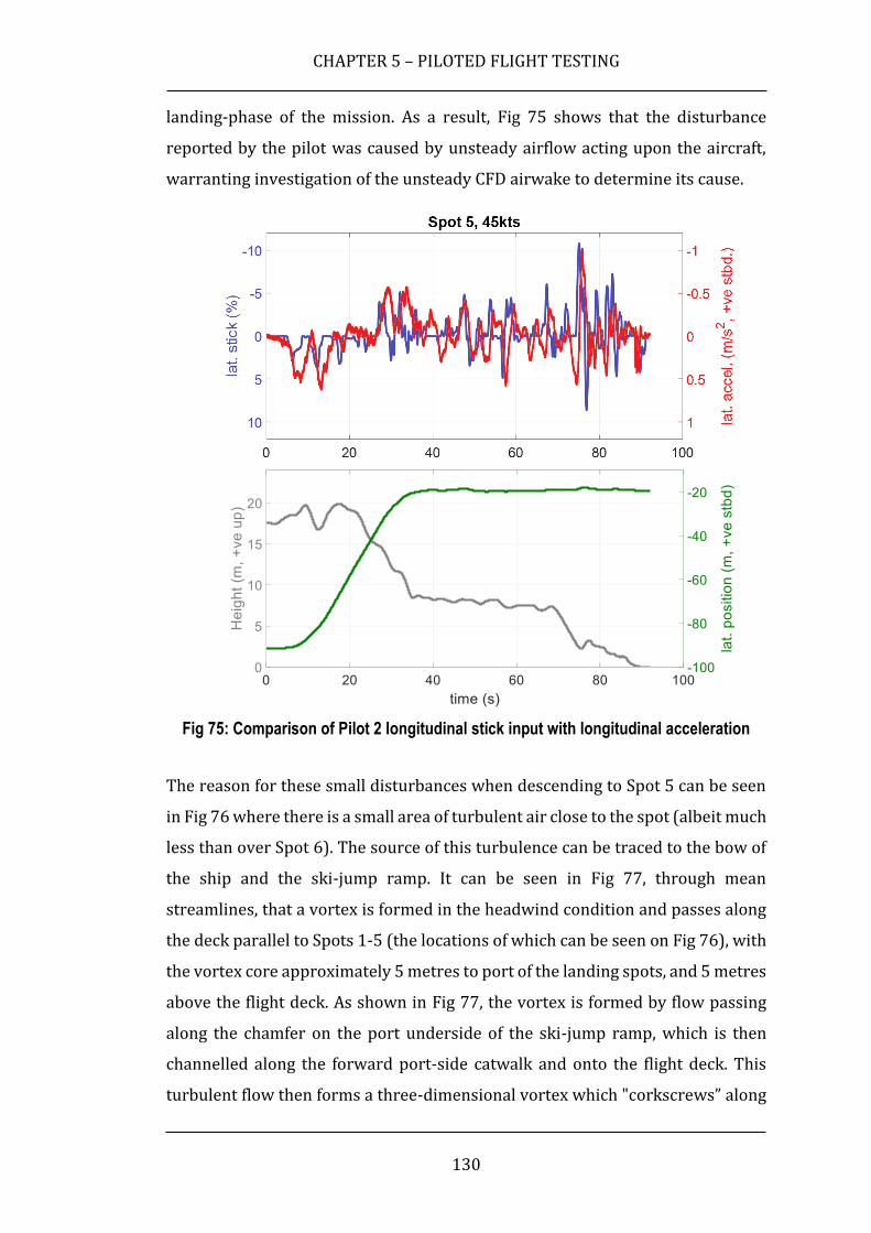
CHAPTER 5 – PILOTED FLIGHT TESTING
130
landing-phase of the mission. As a result, Fig 75 shows that the disturbance
reported by the pilot was caused by unsteady airflow acting upon the aircraft,
warranting investigation of the unsteady CFD airwake to determine its cause.
Fig 75: Comparison of Pilot 2 longitudinal stick input with longitudinal acceleration
The reason for these small disturbances when descending to Spot 5 can be seen
in Fig 76 where there is a small area of turbulent air close to the spot (albeit much
less than over Spot 6). The source of this turbulence can be traced to the bow of
the ship and the ski-jump ramp. It can be seen in Fig 77, through mean
streamlines, that a vortex is formed in the headwind condition and passes along
the deck parallel to Spots 1-5 (the locations of which can be seen on Fig 76), with
the vortex core approximately 5 metres to port of the landing spots, and 5 metres
above the flight deck. As shown in Fig 77, the vortex is formed by flow passing
along the chamfer on the port underside of the ski-jump ramp, which is then
channelled along the forward port-side catwalk and onto the flight deck. This
turbulent flow then forms a three-dimensional vortex which "corkscrews” along

CHAPTER 5 – PILOTED FLIGHT TESTING
131
the port edge of the ski-jump ramp and along landing spots 1-5. Similar vortex
formations have been observed separating from the ski-jump of the Russian
aircraft carrier Admiral Kuznetsov (Maslov, et al., 1998). While, for the QEC, this
vortex had minimal impact upon flight operations at Spot 5 during this trial, it
should be noted that the vortex will have dissipated much of its energy, having
travelled 200 metres along the flight deck prior to reaching Spot 5. A further flight
trial may be warranted to understand the effects of this vortex on flight
operations to Spots 1-4, where the vortex will have more energy and could have
a more significant impact on the aircraft during the latter stages of a landing.
Fig 76: Mean velocity vectors plotted tangential to contours of mean turbulent intensity
Fig 77: Vortex passing along VL Spots 1-5, originating from ski-jump and fwd. port
catwalk

CHAPTER 5 – PILOTED FLIGHT TESTING
132
5.2.1.2 Spot 6
Compared with Spot 5, Bedford workload and DIPES ratings were consistently
higher for Spot 6, as shown in Fig 76. This is a result of the highly unsteady
airwake shedding from the QEC islands upstream of the landing spot. Further, as
a stern approach was used for approaches to Spot 6, both pilots experienced
disturbances to the aircraft throughout MTE1, with Pilot 2 stating “airwake [is]
obvious from the moment [MTE1] started” for Spot 6 at 45kt; this is significant
given that at the beginning of MTE1, the aircraft was positioned 53 metres behind
the stern of the ship.
In addition to the increased workload ratings reported by both pilots, control
input magnitudes could be seen to be increased in comparison with Spot 5,
reflecting the increased corrective control inputs required to compensate for the
increased disturbances to the aircraft. Throughout the manoeuvres to Spot 6, it
was also reported that while “aircraft disturbances [were felt] in all axes”, the
pilots felt the dominant axis to be the pitch axis during station keeping at MTE2.
Analysis of the pilots’ control inputs support this observation, and is shown in Fig
78, where the lateral and longitudinal cyclic inputs are plotted for each WOD to
Spot 5 (blue, left) and Spot 6 (red, right). Control inputs are shown as percentages
of total available control with 50% being the position of the stick at rest, and 0%
and 100% being minimum/maximum limits. While the control inputs come
within 29% of the cyclic-forward longitudinal limit for Spot 6 at 45kt, this is
largely due to the longitudinal trim position required to maintain hover in 25-
45kt wind speed. Longitudinal stick displacement from the trim position does not
significantly exceed lateral stick displacement from trim at any wind speed, with
longitudinal stick displacement and lateral stick displacement having standard
deviations of 4.5% and 4.6% from the trim point respectively. Analysis of lateral
and longitudinal stick control inputs in the single-sided amplitude spectra,
presented in Fig 79, show amplitudes of lateral and longitudinal stick inputs
during hover at Spot 6 (red) compared with those at Spot 5 (blue). Lateral stick
input can again be seen to be the dominant control axis when compared with
Longitudinal stick, with notable increases in control amplitudes at 1.0Hz and

CHAPTER 5 – PILOTED FLIGHT TESTING
133
0.35Hz for lateral stick at Spot 6, due to the turbulence shedding over this landing
spot and disturbing the aircraft.
Fig 78: Pilot 2 cyclic control inputs for MTE2/3 at Spot 5 (blue) and Spot 6 (red)
The collective and pedal control inputs are shown as percentages of total
available control in Fig 80 for Spot 5 (blue), and Spot 6 (red). Each MTE is
separated by an orange marker, allowing a better understanding of variation in
pilot control inputs between MTEs. Comparison of collective inputs shows an
increased standard deviation between Spot 5 and Spot 6 of 5.7%, and 4.7%
respectively, with a minimum 27% and maximum 51% collective control input
for Task 6. This increased variance in collective input was due to increased
disturbance of the aircraft in heave during approach and hover for Spot 6 and
was reported by Pilot 1 as “light ballooning” during MTE1 at 25kt, with Pilot 2
commenting “[I] felt vertical bumps during the mission”.

CHAPTER 5 – PILOTED FLIGHT TESTING
134
Fig 79: Single-Sided Amplitude Spectra of Pilot 2 lateral and longitudinal stick,
collective and pedal control inputs, Ahead 45kt during MTE 2 (hover)
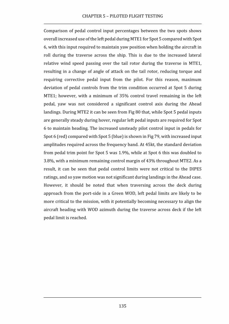
CHAPTER 5 – PILOTED FLIGHT TESTING
135
Comparison of pedal control input percentages between the two spots shows
overall increased use of the left pedal during MTE1 for Spot 5 compared with Spot
6, with this input required to maintain yaw position when holding the aircraft in
roll during the traverse across the ship. This is due to the increased lateral
relative wind speed passing over the tail rotor during the traverse in MTE1,
resulting in a change of angle of attack on the tail rotor, reducing torque and
requiring corrective pedal input from the pilot. For this reason, maximum
deviation of pedal controls from the trim condition occurred at Spot 5 during
MTE1; however, with a minimum of 35% control travel remaining in the left
pedal, yaw was not considered a significant control axis during the Ahead
landings. During MTE2 it can be seen from Fig 80 that, while Spot 5 pedal inputs
are generally steady during hover, regular left pedal inputs are required for Spot
6 to maintain heading. The increased unsteady pilot control input in pedals for
Spot 6 (red) compared with Spot 5 (blue) is shown in Fig 79, with increased input
amplitudes required across the frequency band. At 45kt, the standard deviation
from pedal trim point for Spot 5 was 1.9%, while at Spot 6 this was doubled to
3.8%, with a minimum remaining control margin of 43% throughout MTE2. As a
result, it can be seen that pedal control limits were not critical to the DIPES
ratings, and so yaw motion was not significant during landings in the Ahead case.
However, it should be noted that when traversing across the deck during
approach from the port-side in a Green WOD, left pedal limits are likely to be
more critical to the mission, with it potentially becoming necessary to align the
aircraft heading with WOD azimuth during the traverse across deck if the left
pedal limit is reached.

CHAPTER 5 – PILOTED FLIGHT TESTING
136
Fig 80: Pilot 2 collective and pedal inputs for Spot 5 (blue), and Spot 6 (red), Ahead
45kt. MTEs separated by orange bands
5.3 Flight Trial 2 – Green 25° WOD
Once the Ahead flight trial had been successfully completed, the second flight trial
performed to QEC was for a Green 25° (‘G25°’, i.e. from starboard) WOD
condition, allowing an assessment of how the twin-island design of the QEC will
affect rotary-wing flight operations at different landing spots downwind of the
islands. The G25° WOD was expected to create a significant variation in
turbulence over the QEC port side landing spots, resulting from the variation in
geometry along the upwind starboard side of the ship. As can be seen from Fig
81, which shows ship geometry upwind from each Spot at 30-foot hover height,
Spot 1 has no geometry upwind at hover height, while Spot 2 is almost
downstream of the forward island. Spot 3 can be seen to be downstream of the

CHAPTER 5 – PILOTED FLIGHT TESTING
137
forward island; Spot 4 is downstream of the forward island and gap between the
islands, and Spot 5 is downstream of the aft island. Three wind speeds were again
used: 25kt, 35kt, and 45kt. This gave 30 separate landing attempts during the
G25° flight trial, although due to time constraints Pilot 2 was unable to perform
landings to Spot 1 at the 35kt and 45kt wind speeds, meaning 28 landings were
performed at G25°.
Fig 81: Perspective view looking upwind (G25°) from Spots 1-5, 30ft hover height

CHAPTER 5 – PILOTED FLIGHT TESTING
138
5.3.1 Results
As expected, for the G25° WOD case, it was found that the twin-island design of
the QEC aircraft carriers results in changing pilot workload depending on the
landing spot selected. Spot 4 and Spot 5 were found to have the highest workload
and DIPES ratings on average, with both test pilots assessing these two spots as
being outside the SHOL envelope (DIPES 5) for a 45kt wind speed. Spot 1 was
found to have the lowest pilot workload. An investigation was therefore carried
out by interrogating the CFD results to understand the cause of these high ratings.
For a Green 25° at 25kt wind speed, instantaneous velocity magnitude contours
are displayed in Fig 82 passing over the ship at mean hover height for MTE 2,
overlaid with velocity quivers to give an indication of the flow characteristics
passing over each landing spot. The 16.36 metre SH-60B Seahawk rotor-disc is
also overlaid in Fig 82, located at the mean hover position for MTE 3 at each
landing spot.
Fig 82: Snapshot of instantaneous velocity magnitude over deck at mean hover height
for G25 25kt airwake; SH-60B rotors shown at MTE 3 mean hover point for each landing
spot
Bedford workload and DIPES ratings are presented for Pilot 1 and Pilot 2 in Table
4 and Table 5, respectively. A general comparison between the Bedford workload
and DIPES ratings reported by the two pilots reveals minor differences for the
same conditions, with Pilot 2 tending to report a larger variation in ratings at
both the upper and lower ends of the Bedford scale. As can be seen from Table 4,
Pilot 1 tended to report over a narrower range of Bedford workload ratings,

CHAPTER 5 – PILOTED FLIGHT TESTING
139
awarding scores between four and nine for workload during the trial, while Pilot
2 reported six scores below a rating of four, and eight scores above nine, as per
Table 5. Comparison between the DIPES ratings awarded by the two pilots shows
general agreement, with the exception of Spot 2 at 45kt, which was considered
to be the highest tolerable (DIPES 3) by Pilot 1 (i.e. Acceptable), and outside of
the SHOL envelope (DIPES 5) by Pilot 2 (i.e. Unacceptable). However, the Bedford
workload ratings awarded by the pilots offered better agreement at this spot,
with Pilot 1 considering Spot 2 to have an intolerable (BWR 8) workload at 45kt,
and Pilot 2 gave a similar rating (BWR 9). While DIPES and Bedford ratings
awarded by pilots are subjective, and each pilot will likely experience a different
temporal period of the 30 second airwake (thus potentially causing different
ratings at the same spot), these general trends of variation in pilot perception are
noteworthy and justify the use of more than one pilot as practicable to ensure
reliability in subjective ratings during flight trials. Further discussion is
presented by landing spot, below.
Table 4: Pilot 1 Bedford and DIPES ratings for Spots 1-5, G25° case

CHAPTER 5 – PILOTED FLIGHT TESTING
140
Table 5: Pilot 2 Bedford and DIPES ratings for Spots 1-5, G25° case
5.3.1.1 Spot 1
Due to time constraints during flight testing, Pilot 2 did not perform landings to
Spot 1 at the 35kt and 45kt wind speeds, however a landing was performed at
25kt by Pilot 2, offering an insight into variation of the awarded ratings between
the pilots, as discussed above. Spot 1 was awarded the lowest Bedford workload
and DIPES ratings overall during the G25° trial, with this found to be due to the
landing spot having the lowest levels of turbulence. This lower level of unsteady
airwake can be seen in Fig 83, where contours of turbulence intensity have been
plotted on planes aligned with the freestream flow. As can be seen from Fig 83a,
any turbulence passing over Spot 1 originates from the ski-jump ramp, with flow
being channelled along its vertical starboard edge before passing over Spot 1 at
approximately 2 metres height with turbulence generally remaining below 5%.
There was no perceived increase in pilot workload at Spot 1 during MTE 3, where
this low-level turbulence was experienced during final descent.

CHAPTER 5 – PILOTED FLIGHT TESTING
141
5.3.1.2 Spot 2
Increased levels of turbulence intensity can be seen passing over Spot 2 in Fig
83b, emanating from the forward starboard deck-edge and passing around the
forward island. This turbulent flow can be seen to dissipate in intensity from
approximately 40% down to 23% over the 80 metres between the deck edge and
Spot 2, with mean turbulent intensity being approximately 22-24% over the
rotor disc. These increased levels of turbulence when compared with Spot 1
result in increased Bedford workload and DIPES ratings reported by Pilots 1 and
2, who awarded Bedford ratings of 8 and 9 (workload intolerable for the task)
respectively for the hover task at Spot 2 - 45kt, while at Spot 1 - 45kt the workload
was considered to be ‘tolerable’ at the highest wind speed tested. As can be seen
in Fig 84 and Fig 85, pilot cyclic control inputs increase considerably with wind
speed, due to the increased magnitudes of turbulence passing over the aircraft.
5.3.1.3 Spot 3
Fig 81c shows that for Green 25° winds, Spot 3 is situated in the lee of the QEC
forward island, causing further increased levels of turbulence at this spot relative
to Spot 1 and Spot 2. Turbulence intensity levels can be seen to be around 30%
over the region of the rotor-disc, resulting in increased pilot workload during the
landing. The DIPES ratings awarded by the pilots agreed that, while Spot 3 could
be completed by an average fleet pilot in the 25kt and 35kt WODs, at 45kt this
spot would be ‘Unacceptable’ (DIPES 4-5), and thus unsafe for fleet pilots under
these conditions.
A factor in the awarding of an ‘Unacceptable’ DIPES rating at 45kt was the large
amount of left pedal required to maintain aircraft heading during the traverse
across the deck for MTE1. The left pedal limit was reached during MTE1 for all
spots at 45kt, causing the helicopter to “weather cock” (i.e. an un-commanded
yaw into wind) slightly during the traverse task. This lack of spare yaw control
margin in one axis during the traverse occurred at all landing spots for the 45kt
WOD, and was compensated for by the pilot flying a modified “into wind” task in
which the aircraft heading was aligned with the wind azimuth during MTE1,
thereby recovering some control margin of the aircraft in the yaw axis. Although

CHAPTER 5 – PILOTED FLIGHT TESTING
142
pedal control limits were reached during landings to Spot 3, a frequency domain
analysis of pedal control input in Fig 86 shows this was largely a steady-state
limitation in pedal control, with low amplitude pedal displacements throughout
MTE 2. This phenomenon is best illustrated in Fig 87, which offers a comparison
of collective and pedal inputs at 25kt (in blue) and 45kt (in red). For the landing
to Spot 3 at 45kt, it can be seen that the left pedal limit is reached twice during
the traverse task, with the trim position 13% away from the pedal limit. By
contrast at the 25kt wind speed, the aircraft pedal position is 28% from the limit,
and does not exceed 15% of pedal limits at any point during the manoeuvre.
This reduction in yaw control during the traverse is a feature of helicopters with
an anti-clockwise rotating main rotor and is caused by the increased relative
wind speed passing over the tail rotor as it travels into the wind direction, thus
reducing its thrust and requiring increased levels of pedal input to compensate.
When pedal limits are reached, this loss of tail rotor effectiveness cannot be
compensated for, and so the aircraft will rotate in yaw towards the wind direction
slightly. The pilot compensated for this by aligning aircraft heading into the wind
direction slightly, however with a pedal trim position 13% from the control limit,
pedal inputs frequently came within 10% of pedal limits during the landing
manoeuvre, eroding the ability of the pilot to perform a safe and controlled
landing and thus increasing the awarded DIPES ratings.
5.3.1.4 Spot 4
Mean levels of turbulence intensity at Spot 4 were found to be slightly lower than
those at Spots 3 and 5 for the Green 25° case, being 27% at the hover point; this
minor decrease in airwake unsteadiness was largely due to Spot 4 being
downwind of the gap between the forward and aft islands as shown in Fig 81d.
An increase in turbulence intensity can be observed in Fig 83d where the flow is
passing around the aft island, however this highly turbulent flow then moves out-
of-plane and over Spot 5, leaving Spot 4 relatively less disturbed. However,
perceived pilot workload was not reduced at this spot compared with Spots 3 and
5; indeed, Pilot 1 reported the highest overall DIPES ratings at Spot 4 during the
trial. Pilot 1 deemed the required pilot effort to perform a landing at Spot 4 to be

CHAPTER 5 – PILOTED FLIGHT TESTING
143
‘Excessive’ (DIPES 4-5) for an average fleet pilot at both 35 and 45kt, while Pilot
2 reported this to only be the case at 45kt.
5.3.1.5 Spot 5
The QEC deck landing spot requiring the highest pilot workload according to Pilot
2 was Spot 5, with neither pilot able to complete the landing manoeuvre in the
45kt case. Analysis of the mean turbulence intensity levels at this landing spot in
Fig 83e shows increased levels of unsteady turbulence passing over the deck-
spot at the hover height. Landing Spot 5 is directly downstream of the aft island
for the Green 25° WOD condition, as shown in Fig 81e, with turbulence intensity
levels passing over the area occupied by the rotor-disc shown to be
approximately 29%.

CHAPTER 5 – PILOTED FLIGHT TESTING
144
Fig 83: Contours of mean turbulence intensity plotted on streamwise planes
intersecting the mean hover position for each landing spot

CHAPTER 5 – PILOTED FLIGHT TESTING
145
Fig 84: Pilot 2 cyclic inputs, 90% spatial targets shown in orange - 25kt Green 25°
Fig 85: Pilot 2 cyclic inputs, 90% spatial targets shown in orange - 45kt Green 25°

CHAPTER 5 – PILOTED FLIGHT TESTING
146
Fig 86: Single-Sided Amplitude Spectra of Pilot 2 lateral and longitudinal stick,
collective and pedal control inputs, Green 45° during MTE 2 (hover) to Spot 3

CHAPTER 5 – PILOTED FLIGHT TESTING
147
Fig 87: Comparison of Pilot 2 collective and pedal inputs for Spot 3 for 25kt (blue), and
45kt (red) wind speeds, Green 25°. MTEs separated by orange bands
5.4 Chapter Summary
A high-fidelity flight simulation environment for the UK Royal Navy’s new QEC
aircraft carriers was developed and implemented at the University of Liverpool’s
School of Engineering. This simulation environment was implemented in the
HELIFLIGHT-R piloted flight simulator complete with 6 degree-of-freedom
motion base, and included a realistic QEC visual environment, a mathematical
aircraft model representative of a Sikorsky SH-60B Seahawk, and several CFD
airwake time-histories.

CHAPTER 5 – PILOTED FLIGHT TESTING
148
The purpose of the QEC simulation environment was to demonstrate this new
capability, and to predict the possible effects of the airwake shedding from the
twin-island aircraft carriers on rotary-wing aircraft. An initial flight test was
performed using two experienced former Royal Navy test pilots, with landings
performed to the ship at two wind azimuths (Ahead and Green 25°) and three
wind speeds (25, 35, 45kt).
For both wind directions, it was demonstrated that increasing wind speed causes
increased levels of disturbance to the aircraft, and thus higher levels of pilot
workload during the critical tasks of traversing across deck, station-keeping, and
landing. This increased workload was reflected in both the DIPES and Bedford
workload ratings awarded by the pilots, and from the significantly increased pilot
control activity recorded at higher wind speeds.
The position of each landing spot relative to ship’s geometry also impacted upon
the pilot workload. Generally, it was found that landing spots downwind of ship’s
superstructure for a given WOD condition resulted in increased levels of
disturbance experienced by the aircraft, due to the unsteady airwake shedding
from these features. In the Ahead condition, this resulted in an increased pilot
workload at Spot 6, which is immediately downwind of the ship’s islands;
however, despite this turbulence, Spot 6 was rated by both pilots as being safe
for an average fleet pilot to operate from at all wind speeds tested. In contrast,
Spot 5 was found to be benign at all wind speeds for the Ahead case, with the only
ship’s geometry upwind being the ski-jump ramp, which can be considered an
aerodynamic shape at this azimuth, and therefore does not shed significant levels
of turbulence over Spot 5. For the Green 25° case, Spot 1 was found to be benign
at all wind speeds tested due to their being little in the way of upwind
superstructure, while the pilots experienced varying levels of turbulence at Spots
2-5 at this azimuth, due to the complex flow over and between the QEC twin-
island superstructure and the resultant airwake cascading over the landing spots.
In summary, a high-fidelity flight simulation model of the Royal Navy’s future
flagship has been demonstrated at UoL. Two highly experienced professional
rotary-wing test pilots have performed simulated landings, prior to real-world
FOCFT to the ship, which are planned for 2018. To date, CFD airwakes have been
CHAPTER 5 – PILOTED FLIGHT TESTING
149
generated for 13 different wind azimuths which, when combined with
corresponding ship motions, can be used to simulate full FOCFT to QEC for any
aircraft. This unique capability can be used to provide insight into future FOCFTs
planned for rotary-wing and fixed-wing operations to the QEC.
With the flight trials performed at UoL acting as the final stage of verification for
the newly generated QEC aircraft carrier CFD, these airwakes have now been
delivered to BAE Systems where they have been successfully implemented into
the F-35B ASTOVL simulator at Warton. Simulated FOCFTs have now been
performed for the F-35B Lightning II to the QEC, helping to inform future flight
trials to the ship at sea. While the results of these simulated F-35B trials to QEC
remain confidential, reports of the trials have been widely publicised in the
media (de&s, 2017) (RAeS, 2018).

CHAPTER 6 – CONCLUSIONS AND RECOMMENDATIONS
150
Chapter 6 – Conclusions and Recommendations
This chapter summarises the challenges presented by the development of
aircraft carrier airwakes using CFD for piloted flight simulation and outlines the
research undertaken as described in this thesis. Conclusions are drawn from the
outcomes of this research and a list of recommendations for future work are
presented.
6.1 Conclusions
6.1.1 Aircraft Carrier CFD Generation
The large size of the aircraft carrier CFD airwakes generated in this study
was due to the requirement for fixed-wing operation along the SRVL
glideslope, up to 0.25 miles behind the ship, as well as the requirement for
rotary-wing operation across all areas of the four-acre flight deck.
Turbulence must be accurately resolved and preserved across these areas
of intended flight operation in the computational domain, and so the grid
density must be necessarily refined across this large area of the ship.
Simulation settling time, where the CFD solution requires time to “ramp
up” the turbulent airwake into a periodic flow regime, is significantly
increased for an aircraft carrier. This was found to be a function of the
increased characteristic length of the ship, doubling the required settling
time required for a frigate in an equivalent airwake, and significantly
increasing the required wall-clock time necessary to generate a 30 second
airwake time history.

CHAPTER 6 – CONCLUSIONS AND RECOMMENDATIONS
151
The DDES hybrid formulation of LES and RANS was found to be optimal
for a complex geometry such as an aircraft carrier, because of its improved
resistance to grid induced separation in ambiguous boundary layers. Due
to the difficulty faced in controlling prism first layer height across the
280m ship, the ability of DDES to over-ride the DES limiter and maintain
RANS where required is a useful addition to the original DES formulation.
The requirement to store the large structured and unstructured QEC
airwakes placed significant data storage requirements upon the project,
with each WOD requiring 4.12 TB of secure long-term data storage.
Adequate provision of suitable data storage, in addition to a high-speed
connection to this storage, were found to be critical to the execution of a
high-fidelity aircraft carrier CFD study, and so should be considered
carefully in planning future projects of this scale.
The newly created library of interpolated QEC airwakes were successfully
used by BAE Systems as part of the clearance process for operation of the
Lockheed Martin F-35B Lightning II multirole fighter to the QEC aircraft
carriers, demonstrating their effectiveness in informing future sea trials
to the ship.
6.1.2 Experimental Validation
The inevitable variation in atmospheric freestream conditions which
occurred during the recording of data aboard LHA-5 resulted in some
unphysical effects when comparing wind directions at adjacent points. It
is therefore concluded that the uncertainty around freestream conditions
during testing means that real-world data was not found to be effective
for validation of minor flow features across the ship flight deck, where the
uncertainty of atmospheric conditions can overwhelm minor variations in
the recorded data.
As a result, it was concluded that a bespoke validation experiment is
required to demonstrate fidelity of a CFD solution. The primary advantage
of an experimental arrangement over full-scale data was found to be the
ability to precisely control the inlet conditions in wind and water tunnel

CHAPTER 6 – CONCLUSIONS AND RECOMMENDATIONS
152
facilities, which is essential for CFD validation and not possible using data
from sea trials.
Comparisons between CFD and experiment for the QEC have been found
to be excellent, with good agreement found particularly along the SRVL
glideslope. This is an important finding, as numerical dissipation from the
CFD strategy has been shown to be minimised, with the character of the
airwake preserved up to 0.25 miles downstream of the ship.
6.1.3 QEC Rotary-Wing Flight Testing
For the first trial in the Ahead WOD, increased levels of pilot workload at
Spot 6 were found compared with Spot 5, due to the turbulent flow
shedding from the ships’ bluff-body islands located upstream of Spot 6.
During testing in the Ahead condition at Spot 5, a sudden disturbance to
the aircraft just above deck height was investigated offline and found to
be caused by a longitudinal vortex shedding from the ski-jump ramp and
passing along the length of the flight deck and across Spot 5. Due to the
presence of this vortex at Spot 5, 250 metres downstream of the ski-jump
ramp where it was generated, it can be concluded that numerical
dissipation in the described CFD strategy is adequately low for this
application.
For the second trial in a Green 25° WOD, the trial clearly demonstrated
that the airwake caused by the twin-island layout of QEC can create
unsteady air flow and difficult landing conditions at the downstream
landing spots. This is significant, as the twin-island aircraft carrier
configuration was seen to cause increased turbulence gradients across the
landing spots, compared with the a single-island layout of LHA.
During the flight trials, pilot workload in the Green 25° 45kt WOD
condition was deemed to be too high for an average fleet pilot to land
safely at Spots 3, 4, and 5.

CHAPTER 6 – CONCLUSIONS AND RECOMMENDATIONS
153
6.1.4 General Conclusions
UoL has successfully collaborated with industrial partner BAE Systems to
achieve advances in piloted flight simulation. It is concluded that such co-
operative research projects are mutually beneficial to both industry and
academia.
Initial comparisons between the twin-island QEC and single-island LHA
suggest a single-island configuration may result in increased turbulence
gradients across the landing spots, particularly in Green (i.e. from
starboard) winds. This is significant, as the potential impact of a twin-
island configuration upon pilot workload is not yet understood, and so
further research is recommended to better quantify this difference.
The challenges of generating time-accurate CFD for an aircraft carrier
were found to be considerable, in particular, the increased domain size
and grid density required for a multi-spot ship, and the increased settling
time required to achieve a repeatable solution.
Comparisons with ultrasonic anemometer recordings performed on the
deck of a US Navy helicopter carrier demonstrated the inherent
limitations of using sea trial data to validate CFD, due to the highly
changeable freestream conditions at sea. It is therefore recommended
that wind or water tunnel facilities are preferable to sea trial data for the
purpose of CFD verification and validation.
The ADV flow measurement technique has been demonstrated to be
effective in performing measurements of free shear flow in the lee of a
bluff body. Although this novel approach of using ADV for vehicle wake
analysis has not yet been encountered in the literature, ADV has been
shown to be effective in this application.
Flight simulation was found to be an effective tool in predicting the impact
of turbulent airwake upon piloted landings to an aircraft carrier, prior to
real-world FOCFTs at sea.
Although the present study is now completed, further work around
improving the QEC flight simulation environment and developing
understanding of the ships’ airwake is proposed. Recommendations are
provided in the next section to continue this work.

CHAPTER 6 – CONCLUSIONS AND RECOMMENDATIONS
154
6.2 Recommendations
As the primary role of the QEC aircraft carriers is to provide a fixed-wing
capability to Her Majesty’s Armed Forces, it is recommended that a
mathematical model be developed at UoL to be representative of an
ASTOVL multi-role fighter, allowing investigative fixed-wing trials to be
performed to the ship for both VL and SRVL manoeuvres. Although such
an ASTOVL simulator is in operation at BAE Systems Warton, its
commercial and military classification limits its use in academic research,
and so a generic fixed-wing facility could be developed at UoL for this
purpose.
A further research project is recommended to better understand and
quantify the aerodynamic differences between a single-island and twin-
island aircraft carrier configuration. This should be performed using two
otherwise identical ship geometries, to ensure the differences in airwake
across the two ships are exclusively the result of the islands.
As the UoL CFD interpolation grids were created to encapsulate areas of
VL operation to QEC, the grids do not cover the SRVL glideslope due to the
limited DDR memory dedicated to airwake available in the HELIFLIGHT-
R simulator. Therefore, if an ASTOVL multi-role fighter model is
developed at UoL, so too should a new set of interpolation grids dedicated
to SRVL operation to the ship.
Further experimental data recording using ADV should be performed
around the QEC scale model at different incident angles, to further
reinforce the validation and verification of the CFD airwakes which will be
used to inform future F-35B Lightning II flight trials to the ship.
Due to the difference in Reynolds number between full-scale CFD and
model-scale experimental data, it is recommended that further CFD
around QEC be performed at model scale in the water channel to better
understand how this might affect comparisons between the two data sets.
Incorporation of water channel walls, floor, and free surface in model-
scale CFD would also correct for factors such as blockage in the
experiment, further improving the robustness of the validation strategy
used for the generated full-scale QEC airwakes (it is noted at the time of

CHAPTER 6 – CONCLUSIONS AND RECOMMENDATIONS
155
writing that this recommendation is being implemented with a follow-on
PhD project, referred to in the thesis.

REFERENCES
156
References
ANSYS, 2016. ANSYS FLUENT 16.2 USER GUIDE, Canonsburg, PA: ANYSYS, Inc..
Atkinson, D. C. et al., 2013. Integration of the F-35 Joint Strike Fighter with the UK
QUEEN ELIZABETH Class Aircraft Carrier. Los Angles, CA, International Powered
Lift Conference.
Barlow, J. B., Rae, W. H. & Pope, A., 1999. Low-Speed Wind Tunnel Testing. 3rd ed.
New York, NY: John Wiley & Sons.
Bevilaqua, P. M., 2009. Inventing the F-35 Joint Strike Fighter. Orlando, Florida,
47th. AIAA Aerospace. Sciences Meeting Including the New. Horizons Forum and
Aerospace. Exposition. AIAA 2009-1650.
Blackadar, A. K. & Tennekes, H., 1968. Asymptotic Similarity in Neutral
Barotropic Planetary Boundary Layers. Journal of the Atmospheric Sciences,
25(11), pp. 1015-1020.
Boris, J. P., Grinstein, F. F., Oran, E. S. & Kolbe, R. L., 1992. New insights into Large
Eddy Simulation. Fluid Dynamics Research, 10(4-6), pp. 199-228.
Burt, R. A., 1993. British Battleships 1919-1945. London: Arms and Armour Press.
Carico, G. D. et al., 2003. Helicopter/Ship Qualification Testing, s.l.: NATO RTO-AG-
300-V22.
Chanson, H., 2008. Acoustic Doppler Velocimetry (ADV) In the Field and In
Laboratory: Practical Experiences. Brisbane, Australia, International Meeting on
Measurements and Hydraulics of Sewers.
REFERENCES
157
Chanson, H., Trevethan, M. & Aoki, S., 2008. Acoustic Doppler velocimetry (ADV)
in small estuary: Field experience and signal post-processing. Flow Measurement
and Instrumentation, Volume 19, pp. 307-313.
Chanson, H., Trevethan, M. & Koch, C., 2007. Discussion of "Turbulence
Measurements with Acoustic Doppler Velocimeters" by Carlos M. García, Mariano
I. Cantero, Yarko Niño, and Marcelo H. García. Journal of Hydraulic Engineering,
133(11), pp. 1283-1286.
Charnock, H., 1955. Wind stress on a water surface. Quarterly Journal of the Royal
Meteorological Society, 81(350), pp. 639-640.
Cheney, B. T. & Zan, S. J., 1999. “CFD Code Validation Data and Flow Topology for
The Technical Co-operation Program AER-TP2 Simple Frigate Shape, Ottawa,
Canada: National Research Council Canada, Institute for Aerospace Research.
Chen, W. F. & Lui, E. M., 2005. Handbook of Structural Engineering, Second Edition.
s.l.:CRC Press.
Coles, D., 1956. The law of the wake in the turbulent boundary layer. Journal of
Fluid Mechanics, 1(2), pp. 191-226.
Czerwiec, R. M. & Polsky, S. A., 2004. LHA Airwake Wind Tunnel and CFD
Comparison with and Without Bow Flap. Providence, Rhode Island, 22nd Applied
Aerodynamics Conference and Exhibit, Guidance, Navigation, and Control and
Co-located Conferences.
Darling, K., 2009. Fleet Air Arm Carrier War: The History of British Naval Aviation.
s.l.:Pen And Sword Military.
Davenport, A. G., 1960. Rationale for determining design wind velocities. Journal
of the Structural Division, American Society of Civil Engineers, Volume 86, pp. 39-
68.
de&s, 2017. Front line focus: The F-35 Lightning Simulator. desider, October, pp.
18-19.
Du Val, R. W., 2001. A real-time multi-body dynamics architecture for rotorcraft
simulation. London, UK, American Helicopter Society and Royal Aeronautical
REFERENCES
158
Society International Conference on The Challenge of Realistic Rotorcraft
Simulation.
Du Val, R. W., 2016. FLIGHTLAB: A Suite of Rotorcraft Virtual Engineering Tools,
Liverpool, UK: RAeS Rotorcraft Virtual Engineering Conference.
Dyer, A. J., 1972. A Review of Flux-Profile Relationships. Boundary-Layer
Meteorology, 7(3), pp. 363-372.
Ellis, G. A. & Roscoe, A. H., 1982. The Airline Pilot's View of Flight Deck Workload:
A Preliminary Study Using a Questionnaire, Bedford: Royal Aircraft Establishment.
Forrest, J. S., 2009. Predicting Ship-Helicopter Operating Limits using Time-
Accurate CFD Ship Airwakes and Piloted Flight Simulation. University of Liverpool:
PhD thesis.
Forrest, J. S. & Owen, I., 2010. Investigation of Ship Airwakes using Detached-
Eddy Simulation. Computers & Fluids, 39(4), pp. 656-673.
Forrest, J. S., Owen, I., Padfield, G. D. & Hodge, S. J., 2012. Ship-Helicopter
Operating Limits Prediction Using Piloted Flight Simulation and Time-Accurate
Airwakes. Journal of Aircraft, July-August, Volume 49, pp. 1020-1031.
Friedman, N., 1988. British Carrier Aviation: The Evolution of the Ships and Their
Aircraft. Annapolis, Maryland: Naval Institute Press.
García, C. M., Cantero, M. I., Niño, Y. & García, M. H., 2005. Turbulence
Measurements with Acoustic Doppler Velocimeters. Journal of Hydraulic
Engineering, 131(12), pp. 1062-1073.
Garratt, J. R., 1992. The Atmospheric Bundary Layer. Cambridge: Cambridge
University Press.
Gilbert, M., 2004. The First World War. New York: Holt Paperbacks.
Goring, D. G. & Nikora, V. I., 2002. Despiking Acoustic Doppler Velocimeter Data.
Journal of Hydraulic Engineering, 128(1), p. 117–126.
Healey, J. V., 1991. The Aerodynamics of Ship Superstructures. Seville Spain,
AGARD Conference Proceedings 509: Aircraft Ship Operations.

REFERENCES
159
Henriques, T. et al., 2014. The effects of wave–current interaction on the
performance of a model horizontal axis tidal turbine. International Journal of
Marine Energy, Volume 8, pp. 17-35.
Hinze, J. O., 1975. Turbulence: An Introduction to its Mechanism and Theory,
Second Edition. New York: McGraw-Hill.
Hodge, S. J., 2010. Dynamic Interface Modelling and Simulation Fidelity Criteria.
University of Liverpool: PhD thesis.
Hodge, S. J., Forrest, J. S., Padfield, G. D. & Owen, I., 2012. “Simulating the
environment at the aircraft-ship dynamic interface: research, development, &
application. The Aeronautical Journal, 116(1158), pp. 1155-1184.
Hodge, S. J. & Wilson, P. N., 2008. Operating JSF from CVF: The reality of simulation.
London, UK, RAeS International Powered Lift Conference.
Hodge, S. J. et al., 2009. Time-Accurate and Unsteady Aerodynamic Loads
Modeling for Maritime Helicopter Simulation. Journal of the American Helicopter
Society, 54(2), p. 022005.
Holmes, D. G. & Connell, S. D., 1989. Solution of the 2D Navier-Stokes Equations on
Unstructured Adaptive Grids. Buffalo, NY, USA, s.n.
Hussein, H. J., Capp, S. P. & George, W. K., 1994. Velocity measurements in a high-
Reynolds-number, momentum-conserving, axisymmetrical, turbulent jet. Journal
of Fluid Mechanics, Volume 258, p. 31–75.
Kääriä, C. H., 2012. Investigating the Impact of Ship Superstructure Aerodynamics
on Maritime Helicopter Operations. University of Liverpool: PhD thesis.
Kääriä, C. H., Forrest, J. S., Owen, I. & Padfield, G. D., 2009. Simulated aerodynamic
loading of an SH-60B helicopter in a ship’s airwake. Hamburg, Germany, 35th
European Rotorcraft Forum.
Kääriä, C. H. et al., 2012. Aerodynamic Loading Characteristics of a Model-Scale
Helicopter in a Ship’s Airwake and Implications for Pilot Workload. AIAA Journal
of Aircraft, 49(5), pp. 1271-1278.

REFERENCES
160
Kääriä, C. H., Wang, Y., White, M. D. & Owen, I., 2013. An experimental method for
evaluating the aerodynamic impact of ship superstructures on helicopter
operations. Ocean Engineering, Volume 61, pp. 97-108.
Khorsandi, B., Mydlarski, L. & Gaskin, S., 2012. Noise in Turbulenc Measurements
Using Acoustic Doppler Velocimethry. Journal of Hydraulic Engineering, 138(10),
p. 829–838.
Koch, C. & Chanson, H., 2005. An Experimental Study of Tidal Bores and Positive
Surges: Hydrodynamics and Turbulence of the Bore Front, Brisbane, Australia:
Dept. of Civil Engineering, The University of Queensland.
Kraus, N. C., Lohrmann, A. & Cabrera, R., 1994. New Acoustic Meter for Measuring
3d Laboratory Flows. Journal of Hydraulic Engineering, 120(3), pp. 406-412.
Lee, R. G. & Zan, S. J., 2003. Wind tunnel testing of a helicopter fuselage and rotor
in a ship airwake. Freidrichstrafen, Germany, 29th European Rotorcraft Forum.
Lee, R. G. & Zan, S. J., 2004. Unsteady aerodynamic loading on a helicopter
fuselage in a ship airwake. Journal of the American Helicopter Society, 49(2), pp.
149-159.
Lison, A., 2009. Integrating the Joint Combat Aircraft into the Queen Elizabeth
Class Aircraft Carriers – Design Challenge or Opportunty?. London, UK, RINA
Warship 2009 - Air Power at Sea.
Liu, J., Long, L. N. & Modi, A., 1998. Higher Order Accurate Solutions of Ship Airwake
Flow Fields Using Parallel Computer. Washington, DC, American Helicopter
Society 54th Annual Forum.
Lohrmann, A., Cabrera, R. & Kraus, N., 1994. Acoustic-Doppler Velocimeter (ADV)
for Laboratory Use. Buffalo, New York, Fundamentals and Advancements in
Hydraulic Measurements and Experimentation, American Society of Civil
Engineers.
Lumsden, B. & Padfield, G. D., 1998. Challenges at the helicopter-ship dynamic
interface. London, UK, Military Aerospace Technologies - FITEC ’98, Institution of
Mechanical Engineers.
REFERENCES
161
Martin, V., Fisher, T. S. R., Millar, R. G. & Quick, M. C., 2002. ADV Data Analysis for
Turbulent Flows: Low Correlation Problem. Estes Park, USA, Hydraulic
Measurements and Experimental Methods Specialty Conference (HMEM).
Maslov, L. A., Valuev, N. O. & Zharinov, A. V., 1998. The experience of aerodynamic
disturbances research behind an aircraft-carrier ship with elements for safe
operation of ship-based aircraft. Amsterdam, Netherlands, AGARD symposium on
fluid dynamics, problems of vehicles operating near or in the air–sea interface.
McLelland, S. J. & Nicholas, A. P., 2000. A new method for evaluating errors in
high-frequency ADV measurements. Hydrological Processes, 14(2), pp. 351-366.
Menter, F. R. & Knutz, M., 2004. Adaptation of Eddy-Viscosity Turbulence Models
to Unsteady Separated Flow Behind Vehicles. The Aerodynamics of Heavy
Vehicles: Trucks, Buses, and Trains. Lecture Notes in Applied and Computational
Mechanics, Volume 19, pp. 339-352.
Menter, F. R., Knutz, M. & Langtry, R., 2003. Ten Years of Industrial Experience
with the SST Turbulence Model. Journal of Turbulence, Heat and Mass Transfer,
Volume 4, pp. 625-632.
Millward, A., Nicholson, K. & Preston, J. H., 1980. The use of jet injection to
produce uniform velocity in a high speed water channel. Journal of Ship Research,
Volume 24, pp. 128-134.
Miyake, M. et al., 1970. Comparison of Turbulent Fluxes Over Water Determined
by Profile and Eddy Correlation Techniques. Quarterly Journal of the Royal
Meteorological Society, 96(407), pp. 132-137.
Morton, S. A., Forsythe, J. R., Squires, K. D. & Wurtzler, K. E., 2002. Assessment of
Unstructured Grids for Detached Eddy Simulation of High Reynolds Number
Seperate Flows. Honolulu, Hawaii, 8th International Conference on Numerical
Grid Generation for Compuational Field Simulations, pp. 571-586.
Naval Air Systems Command, 1980. Military Specification Flying Qualities of
Piloted Airplanes, s.l.: MIL-F-8785C.

REFERENCES
162
Naval Air Systems Command, 2001. NATOPS Landing Signal Officer Manual, s.l.:
NAVAIR 00-80T-104.
Navy News, 2012. Wildcat impresses during its first trials aboard a warship.
[Online]
Available at: https://navynews.co.uk/archive/news/item/3691
[Accessed 6 October 2012].
Nezu, I. & Rodi, W., 1986. Open-Channel Flow Measurements with a Laser
Doppler Anemometer. Journal of Hydraulic Engineering, 112(5), pp. 335-355.
Nikora, V. I. & Goring, D. G., 1998. ADV Measurements of Turbulence: Can We
Improve Their Interpretation?. Journal of Hydraulic Engineering, 124(6), pp. 630-
634.
Padfield, G. D., 1996. Helicopter Flight Dynamics. Oxford, UK: Blackwell Science.
Padfield, G. D. & White, M. D., September 2003. Flight Simulation in Academia:
HELIFLIGHT in its First Year of Operation. The Aeronautical Journal, Royal
Aeronautical Society, 107(1075), p. 529 – 538.
Panchapakesan, N. R. & Lumley, J. L., 1993. Turbulence measurements in
axisymmetric jets of air and helium. Part 1. Airjet.. Journal of Fluid Mechanics,
Volume 246, p. 197–223.
Plate, E. J., 1971. Aerodynamic Characteristics of Atmospheric Boundary Layers.
Springfield, VA, USA: U.S. Atomic Energy Commission, Division of Technical
Information.
Polsky, S., 2006. Progress Towards Modeling Ship/Aircraft Dynamic Interface.
Denver, CO, USA, HPCMP Users Group Conference.
Polsky, S. A., 2002. A computational study of unsteady ship airwake. Reno, Nevada,
40th AIAA Aerospace Sciences Meeting & Exhibit.
Polsky, S. A., 2003. CFD Prediction of Airwake Flowfields for Ships Experiencing
Beam Winds. Orlando, Florida, 21st AIAA Applied Aerodynamics Conference.
Polsky, S. A., 2008. NAVAIR Airwake Modelling & More!. Norfolk, VA, HPC User
Group Forum.

REFERENCES
163
Polsky, S. A. & Bruner, C. W. S., 2000. Time-Accurate Computational Simulations of
an LHA Ship Airwake. Denver, CO, USA, AIAA 18th Applied Aerodynamics
Conference and Exhibit.
Polsky, S. A. & Bruner, C. W. S., 2001. A Computational Study of Unsteady Ship
Airwake. Loen, Norway, RTO AVT Symposium on "Advanced Flow Management:
Part A – Vortex Flows and High Angle of Attack for Military Vehicles".
Polsky, S. A. & Ghee, T. A., 2004. Application and Verification of Sub-Grid Scale
Boundary Conditions for the Prediction of Antenna Wake Flowfields. Providence,
Rhode Island, 22nd AIAA Applied Aerodynamics Conference and Exhibit.
Polsky, S. A. & Ghee, T. A., 2008. Application and Verification of Internal Boundary
Conditions for Antenna Mast Wake Predictions. Journal of Wind Engineering and
Industrial Aerodynamics, 96(6-7), pp. 817-830.
Pope, A. & Harper, J. J., 1966. Low Speed Wind Tunnel Testing. 1st ed. New York,
NY: John Wiley & Sons.
Preston, J. H., 1966. The design of high speed, free surface water channels.
Bressanone, Italy, NATO Advanced Study Institute on Surface Hydrodynamics.
RAeS, 2018. Inside F-35B flight test. AEROSPACE, February, pp. 30-33.
Rausch, R. D., Batina, J. T. & Yang, H. T. Y., 1992. Spatial adaptation of unstructured
meshes for unsteady aerodynamic flow computations. AIAA Journal, 30(5), pp.
1243-1251.
Reddy, K. R., Toffoletto, R. & Jones, K. R. W., 2000. Numerical Simulation of Ship
Airwake. Computers & Fluids, 29(4), pp. 451-465.
Rhoades, M. M. & Healey, J. V., 1992. Flight Deck Aerodynamics of a Nonaviation
Ship. Journal of Aircraft, 29(4), pp. 619-626.
Roper, D. M., 2006. Integrating Computational Fluid Dynamics and Piloted
Simulation to Quantify Ship-Helicopter Operating Limits. University of Liverpool:
PhD thesis.

REFERENCES
164
Roper, D. M., Owen, I., Padfield, G. D. & Hodge, S. J., 2006. Integrating CFD and
piloted simulation to quantify ship-helicopter operating limits. The Aeronautical
Journal, 110(1109), pp. 419-428.
Roscoe, A. H., 1984. Assessing Pilot Workload in Flight. Paris, AGARD Conference
Proceedings No.373 Flight Test Techniques.
Roscoe, A. H. & Ellis, G. A., 1990. A Subjective Rating Scale for Assessing Pilot
Workload in Flight: A Decade of Practical Use, Farnborough: Royal Aerospace
Establishment.
Schlichting, H., 1979. Boundary-layer Theory, Seventh Edition. Hamburg: McGraw
Hill.
Shipman, J., Arunajatesan, S., Menchini, C. & Sinha, N., 2005. Ship Airwake
Sensitivities To Modeling Parameters. Reno, Nevada, 43rd Aerospace Sciences
Meeting and Exhibit.
Silva, M. J., Yamauchi, G. K., Wadcock, A. J. & Long, K. R., 2004. Wind Tunnel
Investigation of the Aerodynamic Interactions Between Helicopters and Tilt-rotors
in a Shipboard Environment. San Francisco, CA, American Helicopter Society 4th
Decennial Specialist's Conference on Aeromechanics.
Smith, S. D. & Banke, E. G., 1975. Variation of the sea surface drag coefficient with
wind speed. Quarterly Journal of the Royal Meteorological Society, 101(429), pp.
665-673.
Spalart, P. R. et al., 2006. A new version of detached-eddy simulation, resistant to
ambiguous grid densities. Theoretical and Computational Fluid Dynamics, 20(3),
pp. 181-195.
Spalart, P. R., Jou, W., Strelets, M. & Allmaras, S., 1997. Comments on the feasibility
of LES for wings, and on a hybrid RANS/LES approach. Ruston, LA, USA, Advances
in DNS/LES.
Strelets, M., 2001. Detached Eddy Simulation of Massively Separated Flow. Reno,
NV, USA, AIAA 39th Aerospace Sciences Meeting and Exhibit.

REFERENCES
165
Tedds, S. C., 2014. Scale Model Testing of Tidal Stream Turbines: Wake
Characterisation in Realistic Flow Conditions. University of Liverpool: PhD thesis.
Thornber, B., Starr, M. & Drikakis, D., 2010. Implicit Large Eddy Simulation of Ship
Airwakes. Aeronautical Journal, 114(1162), pp. 715-736.
Urnes, J. M., Hess, R. K. & Moomaw, R. F., 1981. H-Dot Automatic Carrier Landing
System for Approach Control in Turbulence. Journal of Guidance and Control,
4(2), pp. 177-183.
Voulgaris, G. & Trowbridge, J. H., 1998. Evaluation of the Acoustic Doppler
Velocimeter (ADV) for Turbulence Measurements. Journal of Atmospheric and
Oceanic Technology, 15(1), pp. 272-289.
Wahl, T. L., 2000. Analyzing ADV Data Using WinADV. Minneapolis, MN, USA, Joint
Conference on Water Resources Engineering and Water Resources Planning &
Management.
Wahl, T. L., 2003. Discussion of ‘Despiking acoustic Doppler Velocimeter data’ by
Derek G. Goring and Vladimir I. Nikora. Journal of Hydraulic Engineering, 129(6),
p. 484–488.
White, M. D., Dadswell, C., Fell, T. & Coates, R., 2017. The Use of Modelling and
Simulation to Give Students a HEADSTART into Aerospace Engineering. Grapevine,
USA, AIAA Modeling and Simulation Technologies Conference, AIAA SciTech
Forum.
White, M. D. et al., 2012. Acceptance testing and commissioning of a flight
simulator for rotorcraft simulation fidelity research. Proceedings of the IMechE
Part G: Journal of Aerospace Engineering, 227(4), pp. 663-686.
Wieringa, J., 1980. Representativeness of wind observations at airports. Bulletin
of the American Meteorological Society, Volume 61, pp. 962-971.
Wieringa, J. & Rijkoort, P. J., 1983. Windklimaat van Nederland, The Hague: RNMI.
Wilkinson, C. H., Zan, S. J., Gilbert, N. E. & Funk, J. D., 1998. Modelling and
simulation of ship air wakes for helicopter operations-a collaborative venture.

REFERENCES
166
Amsterdam, Netherlands, AGARD symposium on fluid dynamics, problems of
vehicles operating near or in the air–sea interface.
Xia, H. & Qin, N., 2008. DES Applied to an Isolated Synthetic Jet Flow. Notes on
Numerical Fluid Mechanics and Multi-disciplinary Design, Volume 97, pp. 252-260.
Zan, S. J., 2001. Surface Flow Topology for a Simple Frigate Shape. Canadian
Aeronautics and Space Journal, Volume 47, pp. 33-43.
Zan, S. J., 2005. On Aerodynamic Modelling and Simulation of the Dynamic
Interface. Proceedings of the Institution of Mechanical Engineers, Part G: Journal of
Aerospace Engineering, 219(5), pp. 393-410.
ANSYS, 2016. ANSYS FLUENT 16.2 USER GUIDE, Canonsburg, PA: ANYSYS, Inc..
Atkinson, D. C. et al., 2013. Integration of the F-35 Joint Strike Fighter with the UK
QUEEN ELIZABETH Class Aircraft Carrier. Los Angles, CA, International Powered
Lift Conference.
Barlow, J. B., Rae, W. H. & Pope, A., 1999. Low-Speed Wind Tunnel Testing. 3rd ed.
New York, NY: John Wiley & Sons.
Bevilaqua, P. M., 2009. Inventing the F-35 Joint Strike Fighter. Orlando, Florida,
47th. AIAA Aerospace. Sciences Meeting Including the New. Horizons Forum and
Aerospace. Exposition. AIAA 2009-1650.
Blackadar, A. K. & Tennekes, H., 1968. Asymptotic Similarity in Neutral
Barotropic Planetary Boundary Layers. Journal of the Atmospheric Sciences,
25(11), pp. 1015-1020.
Boris, J. P., Grinstein, F. F., Oran, E. S. & Kolbe, R. L., 1992. New insights into Large
Eddy Simulation. Fluid Dynamics Research, 10(4-6), pp. 199-228.
Burt, R. A., 1993. British Battleships 1919-1945. London: Arms and Armour Press.
Carico, G. D. et al., 2003. Helicopter/Ship Qualification Testing, s.l.: NATO RTO-AG-
300-V22.

REFERENCES
167
Chanson, H., 2008. Acoustic Doppler Velocimetry (ADV) In the Field and In
Laboratory: Practical Experiences. Brisbane, Australia, International Meeting on
Measurements and Hydraulics of Sewers.
Chanson, H., Trevethan, M. & Aoki, S., 2008. Acoustic Doppler velocimetry (ADV)
in small estuary: Field experience and signal post-processing. Flow Measurement
and Instrumentation, Volume 19, pp. 307-313.
Chanson, H., Trevethan, M. & Koch, C., 2007. Discussion of "Turbulence
Measurements with Acoustic Doppler Velocimeters" by Carlos M. García, Mariano
I. Cantero, Yarko Niño, and Marcelo H. García. Journal of Hydraulic Engineering,
133(11), pp. 1283-1286.
Charnock, H., 1955. Wind stress on a water surface. Quarterly Journal of the Royal
Meteorological Society, 81(350), pp. 639-640.
Cheney, B. T. & Zan, S. J., 1999. “CFD Code Validation Data and Flow Topology for
The Technical Co-operation Program AER-TP2 Simple Frigate Shape, Ottawa,
Canada: National Research Council Canada, Institute for Aerospace Research.
Chen, W. F. & Lui, E. M., 2005. Handbook of Structural Engineering, Second Edition.
s.l.:CRC Press.
Coles, D., 1956. The law of the wake in the turbulent boundary layer. Journal of
Fluid Mechanics, 1(2), pp. 191-226.
Czerwiec, R. M. & Polsky, S. A., 2004. LHA Airwake Wind Tunnel and CFD
Comparison with and Without Bow Flap. Providence, Rhode Island, 22nd Applied
Aerodynamics Conference and Exhibit, Guidance, Navigation, and Control and
Co-located Conferences.
Darling, K., 2009. Fleet Air Arm Carrier War: The History of British Naval Aviation.
s.l.:Pen And Sword Military.
Davenport, A. G., 1960. Rationale for determining design wind velocities. Journal
of the Structural Division, American Society of Civil Engineers, Volume 86, pp. 39-
68.

REFERENCES
168
de&s, 2017. Front line focus: The F-35 Lightning Simulator. desider, October, pp.
18-19.
Du Val, R. W., 2001. A real-time multi-body dynamics architecture for rotorcraft
simulation. London, UK, American Helicopter Society and Royal Aeronautical
Society International Conference on The Challenge of Realistic Rotorcraft
Simulation.
Du Val, R. W., 2016. FLIGHTLAB: A Suite of Rotorcraft Virtual Engineering Tools,
Liverpool, UK: RAeS Rotorcraft Virtual Engineering Conference.
Dyer, A. J., 1972. A Review of Flux-Profile Relationships. Boundary-Layer
Meteorology, 7(3), pp. 363-372.
Ellis, G. A. & Roscoe, A. H., 1982. The Airline Pilot's View of Flight Deck Workload:
A Preliminary Study Using a Questionnaire, Bedford: Royal Aircraft Establishment.
Forrest, J. S., 2009. Predicting Ship-Helicopter Operating Limits using Time-
Accurate CFD Ship Airwakes and Piloted Flight Simulation. University of Liverpool:
PhD thesis.
Forrest, J. S. & Owen, I., 2010. Investigation of Ship Airwakes using Detached-
Eddy Simulation. Computers & Fluids, 39(4), pp. 656-673.
Forrest, J. S., Owen, I., Padfield, G. D. & Hodge, S. J., 2012. Ship-Helicopter
Operating Limits Prediction Using Piloted Flight Simulation and Time-Accurate
Airwakes. Journal of Aircraft, July-August, Volume 49, pp. 1020-1031.
Friedman, N., 1988. British Carrier Aviation: The Evolution of the Ships and Their
Aircraft. Annapolis, Maryland: Naval Institute Press.
García, C. M., Cantero, M. I., Niño, Y. & García, M. H., 2005. Turbulence
Measurements with Acoustic Doppler Velocimeters. Journal of Hydraulic
Engineering, 131(12), pp. 1062-1073.
Garratt, J. R., 1992. The Atmospheric Bundary Layer. Cambridge: Cambridge
University Press.
Gilbert, M., 2004. The First World War. New York: Holt Paperbacks.

REFERENCES
169
Goring, D. G. & Nikora, V. I., 2002. Despiking Acoustic Doppler Velocimeter Data.
Journal of Hydraulic Engineering, 128(1), p. 117–126.
Healey, J. V., 1991. The Aerodynamics of Ship Superstructures. Seville Spain,
AGARD Conference Proceedings 509: Aircraft Ship Operations.
Henriques, T. et al., 2014. The effects of wave–current interaction on the
performance of a model horizontal axis tidal turbine. International Journal of
Marine Energy, Volume 8, pp. 17-35.
Hinze, J. O., 1975. Turbulence: An Introduction to its Mechanism and Theory,
Second Edition. New York: McGraw-Hill.
Hodge, S. J., 2010. Dynamic Interface Modelling and Simulation Fidelity Criteria.
University of Liverpool: PhD thesis.
Hodge, S. J., Forrest, J. S., Padfield, G. D. & Owen, I., 2012. “Simulating the
environment at the aircraft-ship dynamic interface: research, development, &
application. The Aeronautical Journal, 116(1158), pp. 1155-1184.
Hodge, S. J. & Wilson, P. N., 2008. Operating JSF from CVF: The reality of simulation.
London, UK, RAeS International Powered Lift Conference.
Hodge, S. J. et al., 2009. Time-Accurate and Unsteady Aerodynamic Loads
Modeling for Maritime Helicopter Simulation. Journal of the American Helicopter
Society, 54(2), p. 022005.
Holmes, D. G. & Connell, S. D., 1989. Solution of the 2D Navier-Stokes Equations on
Unstructured Adaptive Grids. Buffalo, NY, USA, s.n.
Hussein, H. J., Capp, S. P. & George, W. K., 1994. Velocity measurements in a high-
Reynolds-number, momentum-conserving, axisymmetrical, turbulent jet. Journal
of Fluid Mechanics, Volume 258, p. 31–75.
Kääriä, C. H., 2012. Investigating the Impact of Ship Superstructure Aerodynamics
on Maritime Helicopter Operations. University of Liverpool: PhD thesis.
Kääriä, C. H., Forrest, J. S., Owen, I. & Padfield, G. D., 2009. Simulated aerodynamic
loading of an SH-60B helicopter in a ship’s airwake. Hamburg, Germany, 35th
European Rotorcraft Forum.

REFERENCES
170
Kääriä, C. H. et al., 2012. Aerodynamic Loading Characteristics of a Model-Scale
Helicopter in a Ship’s Airwake and Implications for Pilot Workload. AIAA Journal
of Aircraft, 49(5), pp. 1271-1278.
Kääriä, C. H., Wang, Y., White, M. D. & Owen, I., 2013. An experimental method for
evaluating the aerodynamic impact of ship superstructures on helicopter
operations. Ocean Engineering, Volume 61, pp. 97-108.
Khorsandi, B., Mydlarski, L. & Gaskin, S., 2012. Noise in Turbulenc Measurements
Using Acoustic Doppler Velocimethry. Journal of Hydraulic Engineering, 138(10),
p. 829–838.
Koch, C. & Chanson, H., 2005. An Experimental Study of Tidal Bores and Positive
Surges: Hydrodynamics and Turbulence of the Bore Front, Brisbane, Australia:
Dept. of Civil Engineering, The University of Queensland.
Kraus, N. C., Lohrmann, A. & Cabrera, R., 1994. New Acoustic Meter for Measuring
3d Laboratory Flows. Journal of Hydraulic Engineering, 120(3), pp. 406-412.
Lee, R. G. & Zan, S. J., 2003. Wind tunnel testing of a helicopter fuselage and rotor
in a ship airwake. Freidrichstrafen, Germany, 29th European Rotorcraft Forum.
Lee, R. G. & Zan, S. J., 2004. Unsteady aerodynamic loading on a helicopter
fuselage in a ship airwake. Journal of the American Helicopter Society, 49(2), pp.
149-159.
Lison, A., 2009. Integrating the Joint Combat Aircraft into the Queen Elizabeth
Class Aircraft Carriers – Design Challenge or Opportunty?. London, UK, RINA
Warship 2009 - Air Power at Sea.
Liu, J., Long, L. N. & Modi, A., 1998. Higher Order Accurate Solutions of Ship Airwake
Flow Fields Using Parallel Computer. Washington, DC, American Helicopter
Society 54th Annual Forum.
Lohrmann, A., Cabrera, R. & Kraus, N., 1994. Acoustic-Doppler Velocimeter (ADV)
for Laboratory Use. Buffalo, New York, Fundamentals and Advancements in
Hydraulic Measurements and Experimentation, American Society of Civil
Engineers.

REFERENCES
171
Lumsden, B. & Padfield, G. D., 1998. Challenges at the helicopter-ship dynamic
interface. London, UK, Military Aerospace Technologies - FITEC ’98, Institution of
Mechanical Engineers.
Martin, V., Fisher, T. S. R., Millar, R. G. & Quick, M. C., 2002. ADV Data Analysis for
Turbulent Flows: Low Correlation Problem. Estes Park, USA, Hydraulic
Measurements and Experimental Methods Specialty Conference (HMEM).
Maslov, L. A., Valuev, N. O. & Zharinov, A. V., 1998. The experience of aerodynamic
disturbances research behind an aircraft-carrier ship with elements for safe
operation of ship-based aircraft. Amsterdam, Netherlands, AGARD symposium on
fluid dynamics, problems of vehicles operating near or in the air–sea interface.
McLelland, S. J. & Nicholas, A. P., 2000. A new method for evaluating errors in
high-frequency ADV measurements. Hydrological Processes, 14(2), pp. 351-366.
Menter, F. R. & Knutz, M., 2004. Adaptation of Eddy-Viscosity Turbulence Models
to Unsteady Separated Flow Behind Vehicles. The Aerodynamics of Heavy
Vehicles: Trucks, Buses, and Trains. Lecture Notes in Applied and Computational
Mechanics, Volume 19, pp. 339-352.
Menter, F. R., Knutz, M. & Langtry, R., 2003. Ten Years of Industrial Experience
with the SST Turbulence Model. Journal of Turbulence, Heat and Mass Transfer,
Volume 4, pp. 625-632.
Millward, A., Nicholson, K. & Preston, J. H., 1980. The use of jet injection to
produce uniform velocity in a high speed water channel. Journal of Ship Research,
Volume 24, pp. 128-134.
Miyake, M. et al., 1970. Comparison of Turbulent Fluxes Over Water Determined
by Profile and Eddy Correlation Techniques. Quarterly Journal of the Royal
Meteorological Society, 96(407), pp. 132-137.
Morton, S. A., Forsythe, J. R., Squires, K. D. & Wurtzler, K. E., 2002. Assessment of
Unstructured Grids for Detached Eddy Simulation of High Reynolds Number
Seperate Flows. Honolulu, Hawaii, 8th International Conference on Numerical
Grid Generation for Compuational Field Simulations, pp. 571-586.

REFERENCES
172
Naval Air Systems Command, 1980. Military Specification Flying Qualities of
Piloted Airplanes, s.l.: MIL-F-8785C.
Naval Air Systems Command, 2001. NATOPS Landing Signal Officer Manual, s.l.:
NAVAIR 00-80T-104.
Navy News, 2012. Wildcat impresses during its first trials aboard a warship.
[Online]
Available at: https://navynews.co.uk/archive/news/item/3691
[Accessed 6 October 2012].
Nezu, I. & Rodi, W., 1986. Open-Channel Flow Measurements with a Laser
Doppler Anemometer. Journal of Hydraulic Engineering, 112(5), pp. 335-355.
Nikora, V. I. & Goring, D. G., 1998. ADV Measurements of Turbulence: Can We
Improve Their Interpretation?. Journal of Hydraulic Engineering, 124(6), pp. 630-
634.
Padfield, G. D., 1996. Helicopter Flight Dynamics. Oxford, UK: Blackwell Science.
Padfield, G. D. & White, M. D., September 2003. Flight Simulation in Academia:
HELIFLIGHT in its First Year of Operation. The Aeronautical Journal, Royal
Aeronautical Society, 107(1075), p. 529 – 538.
Panchapakesan, N. R. & Lumley, J. L., 1993. Turbulence measurements in
axisymmetric jets of air and helium. Part 1. Airjet.. Journal of Fluid Mechanics,
Volume 246, p. 197–223.
Plate, E. J., 1971. Aerodynamic Characteristics of Atmospheric Boundary Layers.
Springfield, VA, USA: U.S. Atomic Energy Commission, Division of Technical
Information.
Polsky, S., 2006. Progress Towards Modeling Ship/Aircraft Dynamic Interface.
Denver, CO, USA, HPCMP Users Group Conference.
Polsky, S. A., 2002. A computational study of unsteady ship airwake. Reno, Nevada,
40th AIAA Aerospace Sciences Meeting & Exhibit.
Polsky, S. A., 2003. CFD Prediction of Airwake Flowfields for Ships Experiencing
Beam Winds. Orlando, Florida, 21st AIAA Applied Aerodynamics Conference.

REFERENCES
173
Polsky, S. A., 2008. NAVAIR Airwake Modelling & More!. Norfolk, VA, HPC User
Group Forum.
Polsky, S. A. & Bruner, C. W. S., 2000. Time-Accurate Computational Simulations of
an LHA Ship Airwake. Denver, CO, USA, AIAA 18th Applied Aerodynamics
Conference and Exhibit.
Polsky, S. A. & Ghee, T. A., 2004. Application and Verification of Sub-Grid Scale
Boundary Conditions for the Prediction of Antenna Wake Flowfields. Providence,
Rhode Island, 22nd AIAA Applied Aerodynamics Conference and Exhibit.
Polsky, S. A. & Ghee, T. A., 2008. Application and Verification of Internal Boundary
Conditions for Antenna Mast Wake Predictions. Journal of Wind Engineering and
Industrial Aerodynamics, 96(6-7), pp. 817-830.
Pope, A. & Harper, J. J., 1966. Low Speed Wind Tunnel Testing. 1st ed. New York,
NY: John Wiley & Sons.
Preston, J. H., 1966. The design of high speed, free surface water channels.
Bressanone, Italy, NATO Advanced Study Institute on Surface Hydrodynamics.
RAeS, 2018. Inside F-35B flight test. AEROSPACE, February, pp. 30-33.
Rausch, R. D., Batina, J. T. & Yang, H. T. Y., 1992. Spatial adaptation of unstructured
meshes for unsteady aerodynamic flow computations. AIAA Journal, 30(5), pp.
1243-1251.
Reddy, K. R., Toffoletto, R. & Jones, K. R. W., 2000. Numerical Simulation of Ship
Airwake. Computers & Fluids, 29(4), pp. 451-465.
Rhoades, M. M. & Healey, J. V., 1992. Flight Deck Aerodynamics of a Nonaviation
Ship. Journal of Aircraft, 29(4), pp. 619-626.
Roper, D. M., 2006. Integrating Computational Fluid Dynamics and Piloted
Simulation to Quantify Ship-Helicopter Operating Limits. University of Liverpool:
PhD thesis.
Roper, D. M., Owen, I., Padfield, G. D. & Hodge, S. J., 2006. Integrating CFD and
piloted simulation to quantify ship-helicopter operating limits. The Aeronautical
Journal, 110(1109), pp. 419-428.

REFERENCES
174
Roscoe, A. H., 1984. Assessing Pilot Workload in Flight. Paris, AGARD Conference
Proceedings No.373 Flight Test Techniques.
Roscoe, A. H. & Ellis, G. A., 1990. A Subjective Rating Scale for Assessing Pilot
Workload in Flight: A Decade of Practical Use, Farnborough: Royal Aerospace
Establishment.
Schlichting, H., 1979. Boundary-layer Theory, Seventh Edition. Hamburg: McGraw
Hill.
Shipman, J., Arunajatesan, S., Menchini, C. & Sinha, N., 2005. Ship Airwake
Sensitivities To Modeling Parameters. Reno, Nevada, 43rd Aerospace Sciences
Meeting and Exhibit.
Silva, M. J., Yamauchi, G. K., Wadcock, A. J. & Long, K. R., 2004. Wind Tunnel
Investigation of the Aerodynamic Interactions Between Helicopters and Tilt-rotors
in a Shipboard Environment. San Francisco, CA, American Helicopter Society 4th
Decennial Specialist's Conference on Aeromechanics.
Smith, S. D. & Banke, E. G., 1975. Variation of the sea surface drag coefficient with
wind speed. Quarterly Journal of the Royal Meteorological Society, 101(429), pp.
665-673.
Spalart, P. R. et al., 2006. A new version of detached-eddy simulation, resistant to
ambiguous grid densities. Theoretical and Computational Fluid Dynamics, 20(3),
pp. 181-195.
Spalart, P. R., Jou, W., Strelets, M. & Allmaras, S., 1997. Comments on the feasibility
of LES for wings, and on a hybrid RANS/LES approach. Ruston, LA, USA, Advances
in DNS/LES.
Strelets, M., 2001. Detached Eddy Simulation of Massively Separated Flow. Reno,
NV, USA, AIAA 39th Aerospace Sciences Meeting and Exhibit.
Tedds, S. C., 2014. Scale Model Testing of Tidal Stream Turbines: Wake
Characterisation in Realistic Flow Conditions. University of Liverpool: PhD thesis.
Thornber, B., Starr, M. & Drikakis, D., 2010. Implicit Large Eddy Simulation of Ship
Airwakes. Aeronautical Journal, 114(1162), pp. 715-736.

REFERENCES
175
Urnes, J. M., Hess, R. K. & Moomaw, R. F., 1981. H-Dot Automatic Carrier Landing
System for Approach Control in Turbulence. Journal of Guidance and Control,
4(2), pp. 177-183.
Voulgaris, G. & Trowbridge, J. H., 1998. Evaluation of the Acoustic Doppler
Velocimeter (ADV) for Turbulence Measurements. Journal of Atmospheric and
Oceanic Technology, 15(1), pp. 272-289.
Wahl, T. L., 2000. Analyzing ADV Data Using WinADV. Minneapolis, MN, USA, Joint
Conference on Water Resources Engineering and Water Resources Planning &
Management.
Wahl, T. L., 2003. Discussion of ‘Despiking acoustic Doppler Velocimeter data’ by
Derek G. Goring and Vladimir I. Nikora. Journal of Hydraulic Engineering, 129(6),
p. 484–488.
White, M. D., Dadswell, C., Fell, T. & Coates, R., 2017. The Use of Modelling and
Simulation to Give Students a HEADSTART into Aerospace Engineering. Grapevine,
USA, AIAA Modeling and Simulation Technologies Conference, AIAA SciTech
Forum.
White, M. D. et al., 2012. Acceptance testing and commissioning of a flight
simulator for rotorcraft simulation fidelity research. Proceedings of the IMechE
Part G: Journal of Aerospace Engineering, 227(4), pp. 663-686.
Wieringa, J., 1980. Representativeness of wind observations at airports. Bulletin
of the American Meteorological Society, Volume 61, pp. 962-971.
Wieringa, J. & Rijkoort, P. J., 1983. Windklimaat van Nederland, The Hague: RNMI.
Wilkinson, C. H., Zan, S. J., Gilbert, N. E. & Funk, J. D., 1998. Modelling and
simulation of ship air wakes for helicopter operations-a collaborative venture.
Amsterdam, Netherlands, AGARD symposium on fluid dynamics, problems of
vehicles operating near or in the air–sea interface.
Xia, H. & Qin, N., 2008. DES Applied to an Isolated Synthetic Jet Flow. Notes on
Numerical Fluid Mechanics and Multi-disciplinary Design, Volume 97, pp. 252-260.

REFERENCES
176
Zan, S. J., 2001. Surface Flow Topology for a Simple Frigate Shape. Canadian
Aeronautics and Space Journal, Volume 47, pp. 33-43.
Zan, S. J., 2005. On Aerodynamic Modelling and Simulation of the Dynamic
Interface. Proceedings of the Institution of Mechanical Engineers, Part G: Journal of
Aerospace Engineering, 219(5), pp. 393-410.

APPENDIX A: PUBLICATIONS
177
Appendix A: Publications
The author has produced the following publications during the pursuit of this
research project:
M. F. Kelly, M. White, I. Owen, S. J. Hodge, “Using airwake simulation to
inform flight trials for the Queen Elizabeth Class Carrier,” in IMarEST 13th
International Naval Engineering Conference and Exhibition, Bristol, UK,
26-28 April 2016.
M. F. Kelly, M. D. White, I. Owen, S. J. Hodge, “The Queen Elizabeth Class
Aircraft Carriers: Airwake Modelling and Validation for ASTOVL Flight
Simulation,” in American Society of Naval Engineers Launch and Recovery
Symposium, Linthicum Heights, Maryland, USA, 16-17 November 2016.
I. Owen, M. White, P. Scott, R. Mateer, M. Kelly, “Modelling and Simulation
at The University of Liverpool in Support of UK Naval Aviation,” in
American Society of Naval Engineers Launch and Recovery Symposium,
Linthicum Heights, Maryland, USA, 16-17 November 2016.
M. F. Kelly, M. D. White, I. Owen, S. J. Hodge, “Piloted Flight Simulation for
Helicopter Operation to the Queen Elizabeth Class Aircraft Carriers,” in
43rd European Rotorcraft Forum and 28th Society of Flight Test Engineers
European Chapter Symposium, Milan, Italy, 12-15 September 2017.
P. Scott, M. F. Kelly, M. D. White, I. Owen, “Using Piloted Simulation to
Measure Pilot Workload of Landing a Helicopter on a Small Ship,” in 43rd
European Rotorcraft Forum and 28th Society of Flight Test Engineers
European Chapter Symposium, Milan, Italy, 12-15 September 2017.