the economics of the nord stream pipeline system
TRANSCRIPT

The Economics of the Nord Stream Pipeline System
Chi Kong Chyong, Pierre Noël and David M. Reiner
September 2010
CWPE 1051 & EPRG 1026
www.eprg.group.cam.ac.uk
EP
RG
WO
RK
ING
PA
PE
R
Abstract
The Economics of the Nord Stream Pipeline System
EPRG Working Paper 1026
Cambridge Working Paper in Economics 1051
Chi Kong Chyong, Pierre Noёl and David M. Reiner
We calculate the total cost of building Nord Stream and compare its
levelised unit transportation cost with the existing options to transport
Russian gas to western Europe. We find that the unit cost of shipping
through Nord Stream is clearly lower than using the Ukrainian route and
is only slightly above shipping through the Yamal-Europe pipeline.
Using a large-scale gas simulation model we find a positive economic
value for Nord Stream under various scenarios of demand for Russian
gas in Europe. We disaggregate the value of Nord Stream into project
economics (cost advantage), strategic value (impact on Ukraine’s transit
fee) and security of supply value (insurance against disruption of the
Ukrainian transit corridor). The economic fundamentals account for the
bulk of Nord Stream’s positive value in all our scenarios.
Keywords Nord Stream, Russia, Europe, Ukraine, Natural gas, Pipeline,
Gazprom
JEL Classification L95, H43, C63
Contact [email protected] Publication September 2010 Financial Support ESRC TSEC 3
1
The Economics of the Nord Stream Pipeline System1
Chi Kong Chyong* Electricity Policy Research Group (EPRG),
Judge Business School, University of Cambridge (PhD Candidate)
Pierre Noёl EPRG, Judge Business School, University of Cambridge
David M. Reiner EPRG, Judge Business School, University of Cambridge
1. The context In 2009 Russia’s natural gas exports to markets in the European Union and
the Commonwealth of Independent States (CIS) generated around 4.5% of
Russia’s GDP, or half of Gazprom’s total revenue.2 Tax receipts from gas exports
amount to 30% of Russia’s defence budget.3 On other hand, one quarter of the
EU’s natural gas consumption, or 6.5% of the bloc’s total primary energy supply,
is covered by Russian gas (Noel, 2008, Noel, 2009). Two countries, Italy and
Germany, account for about half of all contracted Russian exports to the EU, with
France the third biggest importer. The 12 newer member states of Central and
Eastern Europe together represent about a third of all EU imports of Russian gas.
The EU‐Russia gas trade is highly dependent on Ukraine as three‐quarters of
gas exports to Europe transit through Ukrainian pipelines (see Appendix A for
description of Gazprom’s current gas export routes). Russia‐EU gas trade
relations have been complicated by frictions between Russia and the key transit
1 This working paper presents preliminary research findings, and you are advised to cite with caution unless you first contact the author regarding possible amendments. * Corresponding author – ESRC Electricity Policy Research Group, EPRG, University of Cambridge, Judge Business School, email: [email protected] 2 a i This includes revenues from all commercial activities (g s, o l, electricity, transportation and others) of Gazprom and its affiliates. 3 Authors’ own calculations based on Gazprom (2010a) and Russian Federal State Statistics Service (2010)
2
countries on its Western border ‐ Belarus and Ukraine. There have been several
major gas transit disruptions including through Belarus shortly in 2004 and for 3
days in June 2010, and through Ukraine for 4 days in January 2006 and three
weeks in January 2009, including two weeks of total disruption affecting millions
of customers in South‐Eastern Europe and the Western Balkans (Pirani et al.,
2009, Silve, 2009, Kovacevic, 2009).
Since the breakdown of the Soviet Union, Gazprom has pursued a strategy of
diversifying its export options to Europe which began with the construction of
the Yamal‐Europe pipeline in the 1990s (Victor and Victor, 2006). It continued
more recently with the Nord Stream and South Stream projects – under the
Baltic and Black Sea, respectively –promoted by Gazprom and its large west‐
European clients. Once operational, these two projects would have a capacity
larger than the current volume of gas being transported through Ukraine to
Europe.
We focus on an economic analysis of the Nord Stream pipeline system4 (for
details on the project see Appendix B). Our aim is to assess the economic benefits
of the project to its owners and particularly to Gazprom. We will do so in two
steps: first, using detailed analysis of the Nord Stream project (see appendix C)
we derive its total costs and compare the levelised unit transportation cost
through Nord Stream and the existing routes; then we estimate the profits of
Gazprom with and without Nord Stream under various scenarios of gas demand
in Europe, using a computational game‐theoretic model of Eurasian gas trade.
Details on the mathematical formulation of the gas model are provided in
(Chyong and Hobbs, 2010).
The rest of the paper is organized as follows. In the next section, we discuss
the existing economic literature on Nord Stream. Section 3 summarises the
structure and the scope of the model. Then, in Section 4 we briefly discuss some
key market development scenarios used in the analysis. Our results are
presented in Sections 5‐8. We summarise our findings and conclude in Section 9.
4 By Nord Stream pipeline system, or NSPS, we mean all pipelines (including the Gryazovets‐Vyborg pipeline in Russia, Nord Stream offshore pipeline underneath the Baltic Sea, Opal and Nel pipelines in Germany and Gazelle pipeline in the Czech Republic) that are part of the new export route to Europe.
3
2. The existing literature Nord Stream has been politically controversial but there has not been any
attempt – at least publicly available – to examine the economics of the project in
an in‐depth manner and assess whether it is going to be profitable to its owners.
The applied game‐theoretic literature has found some economic rationale for
building a project such as Nord Stream (Hubert and Ikonnikova, 2003, Hubert
and Suleymanova, 2006) and the Yamal‐Europe pipeline (Hirschhausen et al.,
2005). The economic and strategic insights from this literature are valuable,
although authors may have underestimated the value of Nord Stream and the
cost of using the existing transport routes. Hubert and Ikonnikova (2003) and
Hubert and Suleymanova (2006), neglect the changing geography of Russian
production, the expected transition from the traditional fields towards the Yamal
peninsula (Stern, 2009). Nord Stream is a shorter route to transport gas from the
Yamal peninsula to Western Europe than using the Ukrainian corridor and
existing transmission grid in Russia. Therefore, once Gazprom’s production
moves north, the transportation cost through Ukraine will increase.
Using a strategic simulation model of European gas supply, Holz et al. (2009)
find that Russian gas exports to Europe until 2025 would not exceed export
capacity through the existing routes (i.e. 180 bcm/a through Ukraine and
Belarus)5. They conclude that “...the much debated Nordstream pipeline from St.
Petersburg through the Baltic Sea into Germany lacks an economic justification”
(Holz et al., 2009, p.145). However, by suggesting that Nord Stream is
economically justifiable only if Gazprom needs additional export capacity, the
authors imply that shipping gas through Nord Stream would necessarily be more
expensive than using the existing options. Yet they provide no analytical basis to
support this assumption. Explicitly or implicitly, the idea that Gazprom would
need additional net transport capacity to justify Nord Stream economically
stands behind most claims that Nord Stream is a purely geopolitical project (see
for example Christie (2009a) and Christie (2009b)).
5 We should note that the export capacity of the Ukrainian route through Slovakia to Western Europe is 92.6 bcm/a (Naftogaz of Ukraine, 2010). One has to consider this net export capacity when analyzing Nord Stream, not the total transit capacity though Ukraine which is approximately 150 bcm/a.
4
We have not encountered any in‐depth, publically available analysis of the
economics of Nord Stream in the literature, which would allow for a rigorous
comparison of the cost of building and using the new pipeline versus the existing
ransit corridors, and assess the benefits of Nord Stream to its owners. t
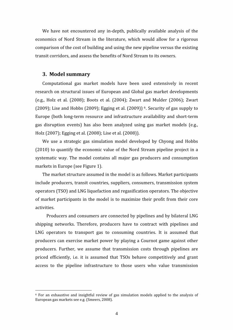
3. Model summary Computational gas market models have been used extensively in recent
research on structural issues of European and Global gas market developments
(e.g., Holz et al. (2008); Boots et al. (2004); Zwart and Mulder (2006); Zwart
(2009); Lise and Hobbs (2009); Egging et al. (2009)) 6. Security of gas supply to
Europe (both long‐term resource and infrastructure availability and short‐term
gas disruption events) has also been analyzed using gas market models (e.g.,
Holz (2007); Egging et al. (2008); Lise et al. (2008)).
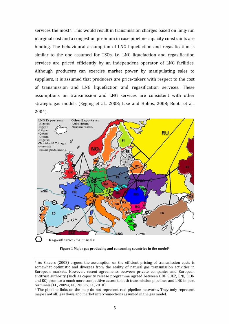
We use a strategic gas simulation model developed by Chyong and Hobbs
(2010) to quantify the economic value of the Nord Stream pipeline project in a
systematic way. The model contains all major gas producers and consumption
markets in Europe (see Figure 1).
The market structure assumed in the model is as follows. Market participants
include producers, transit countries, suppliers, consumers, transmission system
operators (TSO) and LNG liquefaction and regasification operators. The objective
of market participants in the model is to maximize their profit from their core
activities.
Producers and consumers are connected by pipelines and by bilateral LNG
shipping networks. Therefore, producers have to contract with pipelines and
LNG operators to transport gas to consuming countries. It is assumed that
producers can exercise market power by playing a Cournot game against other
producers. Further, we assume that transmission costs through pipelines are
priced efficiently, i.e. it is assumed that TSOs behave competitively and grant
access to the pipeline infrastructure to those users who value transmission
6 For an exhaustive and insightful review of gas simulation models applied to the analysis of European gas markets see e.g. (Smeers, 2008).
5
services the most7. This would result in transmission charges based on long‐run
marginal cost and a congestion premium in case pipeline capacity constraints are
binding. The behavioural assumption of LNG liquefaction and regasification is
similar to the one assumed for TSOs, i.e. LNG liquefaction and regasification
services are priced efficiently by an independent operator of LNG facilities.
Although producers can exercise market power by manipulating sales to
suppliers, it is assumed that producers are price‐takers with respect to the cost
of transmission and LNG liquefaction and regasification services. These
assumptions on transmission and LNG services are consistent with other
strategic gas models (Egging et al., 2008; Lise and Hobbs, 2008; Boots et al.,
2004).
Figure 1 Major gas producing and consuming countries in the model8
7 As Smeers (2008) argues, the assumption on the efficient pricing of transmission costs is somewhat optimistic and diverges from the reality of natural gas transmission activities in European markets. However, recent agreements between private companies and European antitrust authority (such as capacity release programme agreed between GDF SUEZ, ENI, E.ON a lnd EC) promise a much more competitive access to both transmission pipe ines and LNG import terminals (EC, 2009a; EC, 2009b; EC, 2010). 8 The pipeline links on the map do not represent real pipeline networks. They only represent major (not all) gas flows and market interconnections assumed in the gas model.
6
In each consuming country there are a certain number of gas suppliers who
buy gas from producers and re‐sell it to final customers, paying distribution
costs. Following Boots et al. (2004), the operation of suppliers is modelled
implicitly via effective demand curves facing producers in each country9. For this
analysis we assume that suppliers are competitive.
Natural gas prices might differ substantially among countries. Countries that
are closer to gas sources enjoy lower prices than countries that are further from
gas sources, because of the considerable transportation cost including possible
congestion fees on transmission pipelines and transit countries’ mark‐up due to
the exercise of market power. Apart from differences in transport costs, gas
prices can also differ significantly due to different degrees of competition among
producers supplying a particular national market. For example, well diversified
markets in Western Europe have lower prices (on average) than prices enjoyed
by some countries of Central and Eastern Europe (some Central and Eastern
uropean countries have only one source of gas suppliesE
10).
4. Market development assumptions The economics of the Nord Stream project depends greatly on future
developments of gas demand in Europe as well as on the LNG market
developments. In this section, we present three scenarios of European gas
demand and our assumptions about LNG market development.
9 In the derivation of the effective demand curve, suppliers operating in each country are assumed identical. As Smeers (2008) argues, this assumption does not correspond to the reality of European downstream markets. 10 For a detailed discussion of gas markets in Central and Eastern Europe see e.g. Noel (2008) and Noel (2009).

7
Figure 2 Evolution of Gas Demand Outlooks11
A decade of forecasts by the International Energy Agency (IEA) and the US
DOE’s Energy Information Administration (EIA) illustrates the energy experts’
downward trend in their view of future growth in European gas demand (Figure
2). Our base case scenario is based on the IEA’s 2009 forecast (IEA, 2009) while
for our high demand case we average the projected growth rates from the IEA’s
World Energy Outlook (WEO) published between 2000 and 2005. For our low
demand case we assume that European gas consumption would decline 0.2%
annually, similar to the WEO 2009’s “450 Scenario”. (See Table 1).
High Demand
Case
Base Case Low Demand
Case
Western and Southern Europe +2.14% +0.7% ‐0.2%
Central and Eastern Europe +2.14% +0.8% ‐0.2%
Balkan Countries +2.14% +0.8% ‐0.2% Table 1 Assumed growth rat of gas consumption 20102030
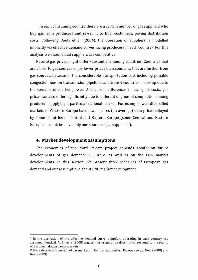
LNG regasification capacities for major gas markets in Europe are
assembled from Gas Strategies Database of LNG regasification terminals up to
2030 (Gas Strategies, 2007). We assume that 50% of all projects announced in
the Gas Strategies database would be realised as it was assembled in 2007
during a period of high gas demand and prices in Europe. The resulting LNG
regasification capacities in Europe are reported in Table 2.
e :
11 This figure is adapted from Noel (2009).
8
2010 2020 2030 2040
UK 43 67 67 67
Germany 0 15 15 15
Netherlands 9 30 30 30
Italy 12 65 65 65
France: Mediterranean 17 17 17 17
France: Atlantic 13 23 23 23
Belgium 9 18 18 18 Table 2 Assumed regasification capacities in major Western European markets (bcm/a)
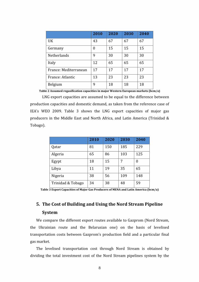
LNG export capacities are assumed to be equal to the difference between
production capacities and domestic demand, as taken from the reference case of
IEA’s WEO 2009. Table 3 shows the LNG export capacities of major gas
producers in the Middle East and North Africa, and Latin America (Trinidad &
obago). T
2010 2020 2030 2040
Qatar 81 150 185 229
Algeria 65 86 103 125
Egypt 18 15 7 0
Libya 11 19 35 65
Nigeria 38 56 109 148
Trinidad & Tobago 34 38 48 59 Table 3 Export Capacities of Major Gas Producers of MENA and Latin America (bcm/a)
5. The Cost of Building and Using the Nord Stream Pipeline
System
We compare the different export routes available to Gazprom (Nord Stream,
the Ukrainian route and the Belarusian one) on the basis of levelised
transportation costs between Gazprom’s production field and a particular final
gas kmar et.
The levelised transportation cost through Nord Stream is obtained by
dividing the total investment cost of the Nord Stream pipelines system by the

9
volumes transported over forty years. We calculate the total investment cost
using the methodology and data described in appendix C. Figure 3 shows the
minimum, the average and the maximum values for each component of the
pipeline system. These figures include the construction cost, the cost of
compressors and the cost of debt financing.
Figure 3 Investment Costs of the Nord Stream system
The total investment costs of the Nord Stream system varies between US$
19.9 bn and US$ 23 bn. As might be expected, the single largest component of the
Nord Stream system is the offshore pipeline underneath the Baltic Sea, which
accou b cnts for a out 56% of the total apital cost of the system.
Table 4 shows the levelised transportation cost for each section of the
pipeline system, assuming they would be fully utilised during their economic life‐
time (results under alternative assumption are also shown later). The figures in
Table 4 represent how much each pipeline should charge in order to pay back its
investment costs, annual O&M costs and earn 1% above the weighted‐average
cost of capital (WACC) for the investors12.
12 The choice to use 1% above WACC is discussed in appendix C.

10
Gryazovets
Vyborg
Nord Stream
Offshore
Opal Gazelle Nel
Levelized
Transport Cost,
$/tcm
Average 28.7 21.2 5.0 2.7 12.8
Max 37.7 28.2 6.4 3.3 15.7
Min 20.9 14.9 3.7 2.1 10.0 Table 4 Levelized Transportation Cost through the Nord Stream system
To compare the Nord Stream system with the Ukrainian and Belarusian
routes we assume that all transit fees (through Belarus, Poland, Ukraine13,
Slovakia and the Czech Republic) would remain at the level of 2009‐2010. The
cost of fuel gas as a component of the transit fee has been omitted from this
analysis.14
Following the International Energy Agency (IEA, 2009) we assume that by
2030 at least 75% of Gazprom’s total gas production would come from new
fields on the Yamal Peninsula.15 This gradual shift of production to the north, as
the Nadym‐Pur‐Taz region declines, has important implications for the relative
costs of the transportation options. It positively affects the competitiveness of
both the Nord Stream and Belarusian routes and disfavours the Ukrainian route.
This is because the distance from the Yamal Peninsula to the Russia‐Ukraine
border is longer than the distance from the Yamal Peninsula to the Nord Stream
entry point (Vyborg) or to the Russia‐ Belarus border (Smolensk).
As shown in Figure 4 building and using the Nord Stream system is cheaper
for Gazprom than using the Ukrainian route. If the Nord Stream system is utilized
at 75%, then, during 2011‐2021, using the Ukrainian route is cheaper. However,
as Gazprom’s production moves to the Yamal Peninsula, it becomes relatively
more expensive to use the Ukrainian route (see table D2 in Appendix D for the
transmission costs between the production sites and the Russian border).
13 We examine alternative transit pricing strategies for Ukraine in Section 8. 14 Most transit/transmission operators in Europe (e.g. BOG in Austria, NET4GAS in Czech Republic, and Eustream in Slovakia) ask shippers to provide fuel gas in kind. In any case, the cost of fuel gas is rather small (e.g., 0.2% of the total transported quantity per 100 km of distance). 15 The (long‐run marginal) cost of developing and producing gas from the Yamal Peninsula has been taken into account in the gas model. However, we are not taking into account possible gas shipments from the Shtokman field due to the high level of uncertainty regarding the implementation of this project.

11
Figure 4 Transportation Costs from Gazprom’s Production Fields to Germany
Comparing the Belarusian and Nord Stream routes is not as
straightforward since the end points differ. We choose to compare the levelised
transportation costs to Greifswald (on the German northern coast) for Nord
Stream with Mallnow (at the German‐Polish border) for the Yamal‐Europe I
pipeline, which are close enough to each‐other.
Since Gazprom owns the Belarusian section of the Yamal‐Europe pipeline,
it pays only 0.49 US$/tcm/100km to Beltransgaz, operator of the Yamal‐Europe
pipeline in Belarus (Ryabkova, 2010). This fee includes only the operatorship
and O&M costs of the pipeline. Therefore, an unbiased comparison between
these two routes should include the capacity cost of the Yamal‐Europe pipeline
as well. Using the same procedure as for the levelised costs, we have calculated
the annualised capacity cost through the Yamal‐Europe I pipeline in Belarus
assuming that it has been fully utilized since it began operation (in 2001).
Various sources have reported the capital cost for Belarusian part to be around
US$1.6 bln excluding any cost of finance (Interfax, 2000). This is similar to the
capital cost of the Yamal‐Europe I pipeline section in Poland, which has almost
the same length and number of compressor stations (Europol Gaz s.a., 2010). We
use this figure to obtain an estimate of the annualized unit capacity cost for the
Belarus section. The result is remarkably similar to those set by the Polish
energy regulator for the Yamal‐Europe pipeline in Poland (€1.108/tcm/100km
in 2009) (A'LEMAR, 2009).

12
The results of these calculations show that the Belarusian route appears to be
less costly than the Nord Stream route (see Figure 4), although only slightly
(~US$7/tcm). It should be noted that we assume transit fees through Belarus
and Poland at the level of 2009. However, there is, of course, no assurance that
the transit fees through Poland and Belarus will not be changed through 2040.
6. The Economic Value of the Nord Stream System The economic value of the Nord Stream system is calculated by comparing
Gazprom’s anticipated total profit between 2011 and 204016 when the Nord
Stream system is built with Gazprom’s profit when Nord Stream is not built. This
is shown in the following equation:
(1)
where PVNS is the present value of Nord Stream system, Profitn+NS is Gazprom’s
annual profit when the Nord Stream system has been built, ACnNS is annualized
total costs of the Nord Stream system as derived from project based‐analysis
(see details in Appendix C) and ProfitnNS is Gazprom’s annual profit in case the
Nord
Stream system has not been built.
Figure 5 shows the economic value of the Nord Stream system under our
three demand scenarios. The black boxes with solid lines represent the
minimum, average and maximum values of the Nord Stream system assuming
average investment costs (the variability is due to the variance in discount rate
only). The dashed lines show the impact on the project’s maximum and
minimum NPV, of capital expenditures reaching their maximum and minimum
value.
In all scenarios analysed, the Nord Stream system has a positive net
present value. Assuming that transit fees and other transportation costs through
existing routes remain unchanged over time, higher gas demand in Europe
increases the economic value of the new pipeline system over its life‐time. The
16 Our analysis covers the economic life of the Nord Stream system, which is assumed to be 30 years (2011‐2040).

13
average NPV of the Nord Stream system is US$4 bln in the low demand case,
US$6.9 bln in the base case and US$20 bln in the high demand case.
In the best case when gas demand in Europe would be relatively high (CAGR
of +2.14%) and the investment costs in the Nord Stream system low, the
economic value of the pipeline could be as high as US$30 bln over the lifetime of
the system. However, even in the worst case (i.e. a combination of the highest
total investment costs and lowest gas demand scenario) the economic value of
the Nord Stream system would still be positive, at around US$ 500 mln over the
ifetime of the pipeline. l
F
igure 5 Economic Value of the Nord Stream system over its life time under different market
scenarios
7. The Impact of Transit Disruption Risks Nord Stream’s sponsors argue that the project will improve the security of
gas supplies to Europe (Nord Stream AG, 2010e, E.ON, 2010, BASF, 2010b, GDF

14
SUEZ, 2010, Gasunie, 2010). This argument has gained traction after the
sust ained disruption of the Ukrainian transit corridor in January 2009.
To quantify the contribution of the Nord Stream pipeline system to the
security of the Russian‐European gas trade, we evaluate the impact of the
unreliability of transit through Ukraine on the economic value of the Nord
Stream pipeline system, or to put it differently, how much Gazprom might save
from reduced transit disruptions once Nord Stream is built. Equation (2) below
computes Nord Stream’s value including the risks of transit disruptions during
the economic life of the pipeline system:
(2)
where PVdNS is the present value of the Nord Stream system under transit
disruption scenario d, Profitn,d+NS is Gazprom’s profit under transit disruption
scenario d when Nord Stream is built, ACnNS is annualized total costs of the Nord
Stream system, Profitn,dNS is Gazprom’s profit under transit disruption scenario d
in case the Nord Stream system has not been built, pn is the probability of transit
disruption through Ukraine in year n and is assumed to be a random variable
with uniform distribution in [0;1]17.
We run our simulation model under two different disruption scenarios for
the Ukrainian route (see table 5).18
17 To simplify the analysis, we assume that probabilities of disruptions in any period are in dependent (e.g. gas transit disruption in 2009 through Ukraine has no effect on probabilities of future disruption through Ukraine.) 18 The disruption scenarios are for analytical purposes only and do not constitute forecasts of transit disruptions through Ukraine. To simplify the analysis, we assume that the probabilities of disruptions in any period are independent (e.g. gas transit disruption in 2009 through Ukraine has no effect on the probability of future disruptions through Ukraine.). Also, we do not distinguish when exactly the disruption would occur during a particular year (winter or summer times), which would require explicit modelling of storage in the gas simulation model. Therefore, the results should be treated as annual average values.

15
Disruption Scenarios Duration of
Disruptions
Frequency of Disruptions Total days of
disruptions
Moderate Disruption Case 3 weeks 5 disruptions in 2011‐2040 105 days
Severe Disruption Case 6 weeks 10 disruptions in 2011‐2040 420 days Table 5 Transit Disruption Scenarios through Ukraine
Figure 6 presents the results under different scenarios of demand growth
in Europe.
Figur f dee 6 Expected Economic Value o the Nord Stream system un r transit disruption scenarios19
Under the low demand scenario and without any disruption the average
NPV of the system is US$ 3.8 bn. In the moderate disruption case, the expected
additional NPV of the system, reflecting its security value, is US$89 mln, or about
2% of the maximum achievable NPV of the system. Under the severe transit
disruption scenario, the security value of the Nord Stream system would be
US$368 mln (89.4+278.9), or 9% of the maximum possible value.
Under all demand scenarios analyzed at least 90% of the NPV of the pipeline
system comes from the economic fundamentals of the project – lower
transportation cost compared to the existing export routes; the security value of
the project never represents more than 9% of the expected total value. 19 The values inside the bars are the average values of the NPV in US$ bln (equivalent to the middle lines of the solid boxes in figure 5).

16
8. The impact f Ukraine’s Transit Pricing Decisions We have so far assumed that the Ukrainian transit fee over time is
determined according to the long‐term transit contract
o
20 signed after the
January 2009 gas crisis. However, one would think that Ukraine would respond
to the emergence of a new competing option by adapting its transit fee. If the
quantity of gas transported through Ukraine decreases (e.g. because of diversion
of gas flows to the Nord Stream system) then Ukraine’s rational reaction would
be to slash its transit fee so that it would be more profitable for Gazprom to
export gas through the Ukrainian route than through the bypass pipeline21.
Conversely, increased demand for transportation through Ukraine would allow it
to charge a higher fee.
In this section we quantify the impact of Ukraine’s transit pricing decisions
on the economic value of the Nord Stream system22. We compare, under our
three demand scenarios, the value of Nord Stream when the Ukrainian transit fee
is fixed, to its value when the transit fee is a function of Gazprom’s demand for
transit services through Ukraine (that is, a function of the gas transported
through Ukraine, for details see appendix E).
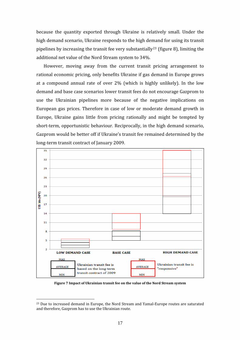
Figure 7 shows the value of the Nord Stream system when the Ukrainian
transit fee is fixed (based on the long‐term transit contract) and when the fee
responds to the construction of the ‘bypass’ pipeline. A responsive Ukrainian fee
has a positive impact on the NPV of the Nord Stream pipeline system, all the
greater than gas consumption growth in Europe is stronger. Under the base case
demand scenario, Ukraine’s rational pricing behaviour increases the value of
Nord Stream by 67%. In the low demand case the impact of Ukraine’s transit
pricing policy increases the value of the Nord Stream system by 29% ‘only’,
20 The full text (in Russian) of the contract has been published on the website of Ukrainian newspaper “Ukrainska Pravda” shortly after its signature (Ukrainska Pravda, 2009). 21 The implicit assumption here is that Gazprom has bargaining power vis‐à‐vis Ukraine, which, in light of recent and also past developments of Russo‐Ukrainian gas relations, seems justifiable. 22 For our future research we will include another scenario – Gazprom acquisition of Naftogaz of Ukraine. Indeed, Ukrainian government officials have explicitly acknowledged that they cannot “stop” the construction of Nord Stream, as it has already started, and therefore, the Ukrainian government has suggested that Gazprom and European gas companies invest in refurbishing Ukrainian transit pipelines and co‐manages the transit system instead of constructing the second “bypass” pipeline – South Stream (Korrespondent.net, 2010).
17
because the quantity exported through Ukraine is relatively small. Under the
high demand scenario, Ukraine responds to the high demand for using its transit
pipelines by increasing the transit fee very substantially23 (figure 8), limiting the
additional net value of the Nord Stream system to 34%.
However, moving away from the current transit pricing arrangement to
rational economic pricing, only benefits Ukraine if gas demand in Europe grows
at a compound annual rate of over 2% (which is highly unlikely). In the low
demand and base case scenarios lower transit fees do not encourage Gazprom to
use the Ukrainian pipelines more because of the negative implications on
European gas prices. Therefore in case of low or moderate demand growth in
Europe, Ukraine gains little from pricing rationally and might be tempted by
short‐term, opportunistic behaviour. Reciprocally, in the high demand scenario,
Gazprom would be better off if Ukraine’s transit fee remained determined by the
long‐term transit contract of January 2009.
Figure 7 Impact of Ukrainian transit fee on the value of the Nord Stream system
23 Due to increased demand in Europe, the Nord Stream and Yamal‐Europe routes are saturated and therefore, Gazprom has to use the Ukrainian route.

18
Figure 8 Ukraine’s transit fee under different assumptions and scenarios
*
Endogenous
9. Summary and conclusions Three factors contribute to the positive economic value of the Nord Stream
pipeline system: the lower transportation cost compared to existing options (the
economic fundamentals of the project); the impact of Nord Stream on lowering
Ukraine’s transit fee; the insurance against transit disruption risks through
Ukraine.
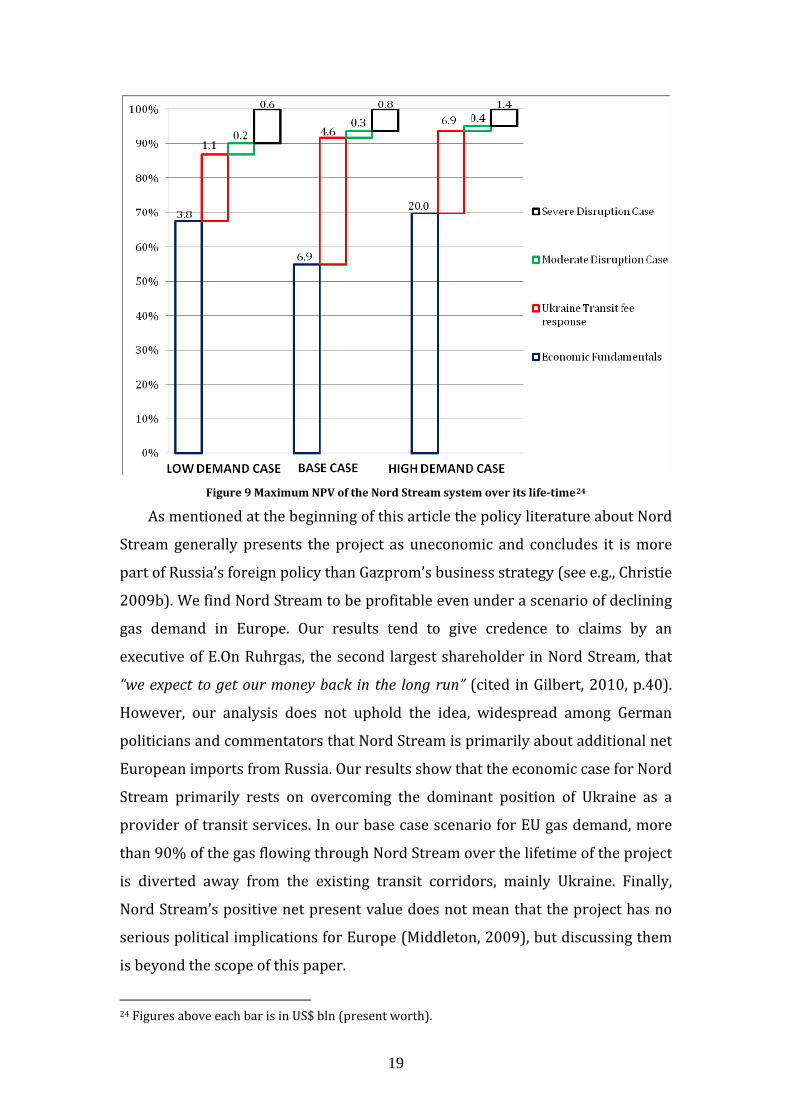
Our results show (Figure 9) that the economic fundamentals guarantee that
the pipeline’s owners will get 55% of the maximum achievable net present value
under the base case demand scenario. In the low and high demand cases, the
economic fundamentals of the project contribute about 70% to the maximum
achievable project value. If Ukraine reduces its transit fee because of the building
of Nord Stream, this is worth 35% of the maximum achievable value of the
project in the base case demand scenario, about 20% and 25% for the low and
high demand cases respectively. The contribution of the insurance against transit
disruption to the value of Nord Stream is relatively modest at about 12% in the
low demand case and less than 10% in the two other scenarios.
19
Figure 9 Maximum NPV of the Nord Stream system over its lifetime24
As mentioned at the beginning of this article the policy literature about Nord
Stream generally presents the project as uneconomic and concludes it is more
part of Russia’s foreign policy than Gazprom’s business strategy (see e.g., Christie
2009b). We find Nord Stream to be profitable even under a scenario of declining
gas demand in Europe. Our results tend to give credence to claims by an
executive of E.On Ruhrgas, the second largest shareholder in Nord Stream, that
“we expect to get our money back in the long run” (cited in Gilbert, 2010, p.40).
However, our analysis does not uphold the idea, widespread among German
politicians and commentators that Nord Stream is primarily about additional net
European imports from Russia. Our results show that the economic case for Nord
Stream primarily rests on overcoming the dominant position of Ukraine as a
provider of transit services. In our base case scenario for EU gas demand, more
than 90% of the gas flowing through Nord Stream over the lifetime of the project
is diverted away from the existing transit corridors, mainly Ukraine. Finally,
Nord Stream’s positive net present value does not mean that the project has no
serious political implications for Europe (Middleton, 2009), but discussing them
is beyond the scope of this paper.
24 Figures above each bar is in US$ bln (present worth).

20
REFERENCES A'LEMAR. 2009. Rossiyskiy rynok aksiy. Ezhednevniy bulleten investora (in
Russian) [Online]. Available: ed http://www.alemar.ru/upload/iblock/918/Facts_021109.pdf [Access
21 November 2010]. ANDERS, T., JOHNSON, P. E. & RAM‐WALLOOPPILLAI, P. E. 2006. The Art and
Science of Designing a Greenfield Pipeline. Pipeline Simulation Interest Group [Online]. Available: http://www.psig.org/Papers/papers.asp [Accessed December 01, 2009].
BARINOV, A. E. 2007. Systemic and Political Factors Affecting Cost Overrun in the Russian Economic World Economy’s Large Investment Projects. Studies on
Development, 18, 8. BASF. 2007. Debt Issuance Programme Prospectus. Available:
http://www.basf.com/group/corporate/de/function/conversions:/publish/content/investor‐relations/bonds‐and‐credit‐rating/images/BASF_DIP_e.pdf [Accessed 9 June 2010].
BASF. 2009. BASF Report 2009 ‐ Economic, environmental and social performance. Available: http://www.basf.com/group/corporate/en/function/conversions:/publi
tent/about‐basf/facts‐sh/conreports/reports/2009/BASF_Report_2009.pdf [Accessed 4 May 2010].
BASF. 2010a. BASF We earn a premium on our cost of capital [Online]. Available: www.basf.com/grou estor‐http:// p/corporate/en/inv
relations/strategy/cost‐of‐capital/index [Accessed 9 June 2010]. BASF. 2010b. Natural Gas Trading [Online]. Available:
tsanalysis/segments/oilgas10].
http://report.basf.com/2009/en/managemen/naturalgastrading.html [Accessed 21 June 20
BERNOTAT, W. 2010. E.ON ‐ 2009 Full Year Results. presentation [Online]. Available: http://www.eon.com/en/downloads/E.ON_Charts_Bernotat_IR.pdf [Accessed 9 April 2010].
BOOTS, M. G., RIJKERS, F. A. M. & HOBBS, B. F. 2004. Trading in the Downstream pean Gas Market: A Successive Oligopoly Approach. The Energy Euro
Journal, 25, 73‐102. CBR. 2010. Official exchange rate of the Central Bank of the Russian Federation
ine]. Available: http://www.cbr.ru cessed 23 [Onl /eng/daily.aspx [AcAugust 2010].
CFE. 2010. Corporate Income Tax in Germany [Online]. Available: y http://www.cfe‐eutax.org/taxation/corporate‐income‐tax/german
[Accessed 21 June 2010]. CHRISTIE, E. 2009a. European security of gas supply: A new way forward. In:
tion: Pipes, Politics anLIUHTO, K. (ed.) The EU‐Russia Gas Connec d Problems ed.: Pan‐European Institute, Turku School of Economics.
CHRISTIE, E. H. 2009b. The battle of Nord Stream. Baltic Rim Economies, 5. CHYONG, C. K. & HOBBS, B. F. 2010. Partial Equilibrium Gas Simulation Model for
Energy Security and Policy Analysis. EPRG Working Paper series forthcoming.
21
E.ON. 2010. Nord Stream Pipeline [Online]. Available: ://www.eon.com/en/businessareas/35301.jsp [Accessed 21 June ].
http2010
EC. 2009a. Antitrust: Commission accepts commitments by GDF Suez to boost competition in French gas market [Online]. Brussels. Available: http://europa.eu/rapid/pressReleasesAction.do?reference=IP/09/1872&
at=HTML&aged=0&language=EN&guiLanguage=en [Accessed July ].
form2010
EC. 2009b. Antitrust: Commission welcomes E.ON proposals to increase competition in German gas market [Online]. Brussels. Available: http://europa.eu/rapid/pressReleasesAction.do?reference=MEMO/09/5
format=HTML&aged=0&language=EN&guiLanguage=en [Accessed 2010].
67&July
EC. 2010. Commission welcomes ENI's structural remedies proposal to increase competition in the Italian gas market [Online]. Brussels. Available: http://europa.eu/rapid/pressReleasesAction.do?reference=SPEECH/10/
ed 19&format=HTML&aged=0&language=EN&guiLanguage=en [AccessJuly 2010].
ECT 2006. Gas Transit Tariffs in selected Energy Charter Treaty Countries. Brussels: Energy Charter Secretariat.
EGGING, R., GABRIEL, S. A., HOLZ, F. & ZHUANG, J. 2008. A Complementarity Model for the European Natural Gas Market. Energy Policy, 36, 2385‐2414.
L, S. 2009. Representing EGGING, R., HOLZ, F., HIRSCHHAUSEN, C. V. & GABRIEGASPEC with the World Gas Model. The Energy Journal, 30, 97‐117.
EIA. 2010. FSU Energy Map 2007 [Online]. Available: ww.eia.doe.gov/cabs/Russia/images/Russian%20Energy%20at
0]. http://w%20a%20Glance%202007.pdf [Accessed June 201
ENTSOG. 2010. The European Natural Gas Network (Capacities at crossborder points on the primary market) [Online]. Available:
g.eu/download/maps_data/ENTSOG_CAP_June2010.pdhttp://www.entsof [Accessed 25 July 2010 2010].
EUROPOL GAZ S.A. 2010. Financing Capital Investment [Online]. Available: ww.europolgaz.com.pl/english/finanse_naklady.h sed 10].
http://w tm [Acces21 April 20
FRUNZE. 2010. NPO izgotovilo oborudovanie dlya SEG (in Russian) [Online]. Available: http://www.frunze.com.ua/index.php?option=com_content&view=article
‐news&Itemid=118 &id=267:2010‐02‐03‐06‐21‐09&catid=1:latest[Accessed 21 April 2010].
GAS STRATEGIES. 2007. LNG Data service. Available: /information‐services/lng‐data‐ember 2008].
http://www.gasstrategies.comro [Accessed 11 Decnual Report 2009.
service/intGASUNIE 2010. AnGAZPROM. 2005. BOARD OF DIRECTORS REVIEWS PRELIMINARY OPERATING
HIGHLIGHTS OVER 2005 AND MAJOR DRAFT FINANCIAL DOCUMENTS FOR 2006 [Online]. Available: http://www.gazprom.com/press/news/2005/november/article63315/ [Accessed 5 June 2010].

22
GAZPROM. 2010a. Gazprom's Databook 2009 [Online]. Available: _28_gazprom_dahttp://www.gazprom.com/f/posts/05/285743/2010_04
tabook_1.xls [Accessed June 21 2010]. GAZPROM. 2010b. Gryazovets – Vyborg gas pipeline. Available:
sed June http://gazprom.com/f/posts/69/824859/img31012.jpeg [Acces2010].
GAZPROM. 2010c. Summary ‐ Portovaya compressor station. Available: w.gazprom.com/f/posts/86/569604/portovaya_eng.pdf http://ww
[Accessed 17 May 2010]. GDF SUEZ. 2010. Press Releases "GDF SUEZ delivers solid results in the first half
and confirms targets" [Online]. Available: .gdfsuez.com/en/news/press‐releases/press‐http://www
releases/?communique_id=1298 [Accessed 11 August 2010]. GILBERT, J. 2010. Continuity and Contradiction: German Energy Company and
European Energy Policy. MPhil in International Relations, University of Cambridge.
HIRSCHHAUSEN, C. V., MEINHART, B. & PAVEL, F. 2005. Transporting Russian Gas to Western Europe ‐ A Simulation Analysis. The Energy Journal, 26, 49‐68.
et? HOLZ, F. 2007. How Dominant is Russia on the European Natural Gas MarkResults from Modeling Exercises. Applied Economics Quarterly.
HOLZ, F., HIRSCHHAUSEN, C. V. & KEMFERT, C. 2008. A strategic model ofEuropean gas supply (GASMOD). Energy Economics, 30, 766‐788.
HOLZ, F., HIRSCHHAUSEN, C. V. & KEMFERT, C. 2009. Perspectives of the European Natural Gas Markets Until 2025. The Energy Journal, 30, 137‐150.
HUBERT, F. & IKONNIKOVA, S. 2003. Strategic investment and bargaining power in supply chains: A Shapley value analysis of the Eurasian gas market. Humboldt University Berlin.
HUBERT, F. & SULEYMANOVA, I. 2006. Strategic investment in international gas‐transport systems: A dynamic analysis of the hold‐up problem. Humboldt University Berlin.
HUBERT, F. & SULEYMANOVA, I. 2008. Strategic Investment in International Gas Transport Systems: A Dynamic Analysis of the Hold‐up Problem DIW
Discussion Papers. IEA 2009. World Energy Outlook 2009. Paris: OECD/International Energy
Agency. SSIAN STRETCH OF YAMAL‐EUROPE GAS PIPELINE TO
ort. INTERFAX 2000. BELARU
BE BUILT IN FIRST HALF OF 2001. Daily Petroleum RepKORCHEMKIN, M. 2010. Nord Stream: Russian land section nearly three times
man OPAL [Online]. Available: ccessed 5 June 2010].
more expensive than Gerhttp://www.eegas.com/pipecost2010‐05e.htm [A
KORRESPONDENT.NET. 2010. Yanukovich schitaet Ukrainskuyu GTS alternativoy Uzhnomu Potoku (in Russian) [Online]. Available:
25 http://korrespondent.net/business/economics/1069560 [AccessedApril 2010].
KOVACEVIC, A. 2009. The Impact of the Russia–Ukraine Gas Crisis in South Eastern Europe. Oxford Institute for Energy Studies Working Papers. Oxford, UK.

23
KPMG. 2009. KPMG in the Czech Republic ‐ Tax Card 2009. Available: ed http://www.kpmg.cz/czech/images/but/0903_Tax‐Card.pdf [Access
25 March 2010]. KREY, V. & MINULLIN, Y. 2010. Modelling competition between natural gas
pipeline projects to China. International Journal of Global EnvironmentalIssues, 10, 143‐171.
as .
LISE, W. & HOBBS, B. F. 2008. Future evolution of the liberalised European gmarket: Simulation results with a dynamic model. Energy, 33, 989‐1004
LISE, W. & HOBBS, B. F. 2009. A Dynamic Simulation of Market Power in the Liberalised European Natural Gas Market. The Energy Journal, 30, 119‐136.
LISE, W., HOBBS, B. F. & OOSTVOORN, F. V. 2008. Natural gas corridors between the EU and its main suppliers: Simulation results with the dynamic GASTALE model. Energy Policy, 36, 1890‐1906.
MANGHAM, C. 2009. Nord Stream financing to sign in December‐bankers. Reuters News Agency [Online]. Available:
rs.com/article/idUKGEE5AM2BP20091123 [Accessed 18 http://uk.reuteJanuary 2010].
help to the European Common , College of Europe.
MIDDLETON, C. 2009. Nord Stream: hindrance or Energy Policy? Master of European Studies
MÜLLER‐STUDER, L. 2009. Zug : doing business. Economic Promotion Zug [Online]. Available: http://www.zug.ch/behoerden/volkswirtschaftsdirektion/economic‐promotion/faq‐frequently‐asked‐questions/economy‐
60bcfa6da3ab6c73e76a3f89/at_download/file 18/resolveUid/496a1826[Accessed 2010].
NAFTOGAZ OF UKRAINE. 2010. Proektni parametry ta faktychni obsyagy transportuvanya prirodnogo gazu gazotransportnoyu systemou Ukrainy: 2008 and 2009 (In Ukrainian) [Online]. Available:
f/0/0DF906D861E53FC7http://www.naftogaz.com/www/2/nakweb.nsC22573FE003F3D66/$file/GTSUkraine.gif [Accessed 21 April 2010].
NAZAROVA, Y. 2009. "Gazprom" menyaet orientatsiu. РБК daily [Online]. /14/tek/4Available: http://www.rbcdaily.ru/2009/09 30898 [Accessed 5
November 2009]. NAZAROVA, Y. 2010. Truboprovodchik "Gazprom". РБК daily [Online]. Available:
.rbcdaily.ru/2010/01/27/tek/454812 [Accessed 23 March http://www2010].
NEFTEGAZ. 2010. Nord Stream pipeline costs will be more expensive than predicted [Online]. Available:
ary http://www.neftegaz.ru/en/news/view/93646/ [Accessed 4 Febru2010].
NEL. 2010. NEL in Zahlen (in German) [Online]. Available: http://www.nel‐.html [Accessed 15 June pipeline.de/public/nel/projekt/opal‐in‐zahlen
2010]. NET4GAS. 2010. Project GAZELLE [Online]. Available:
http://www.net4gas.cz/en/projekt‐gazela/ [Accessed 15 June 2010]. NOEL, P. 2008. Beyond dependence: How to deal with Russian gas. European
Council on Foreign Relations.

24
NOEL, P. 2009. A Market Be cing the Political Cost of Europe’s Dependence on Russian Gas. EPRG Working Paper
& Figures [Online]. Available: http://www.nord‐ 2010].
tween us: Redu
NORD STREAM AG. 2010a. Factsstream.com/en/the‐pipeline/facts‐figures.html [Accessed 15 June
NORD STREAM AG. 2010b. Offshore Advantages [Online]. Available: http://www.nord‐stream.com/en/test/pipeline‐route0/offshore‐advantages0.html [Accessed June 4 2010].
NORD STREAM AG. 2010c. Our Company [Online]. Available: http://www.nord‐stream.com/en/our‐company.html [Accessed 21 June 2010].
NORD STREAM AG. 2010d. The Planned Nord Stream Pipeline Route. Available: http://www.nord‐
in/Dokumente/3__PNG_JPG/4__Maps/The_Planned_Pstream.com/fileadmipeline_Route_EN_rgb.jpg [Accessed June 2010].
NORD STREAM AG. 2010e. Project Significance [Online]. Available: ance.html http://www.nord‐stream.com/en/the‐pipeline/project‐signific
[Accessed April 21 2010]. OPAL. 2010. The OPAL in figures [Online]. Available: http://www.opal‐
pipeline.com/public/en/project/opal‐in‐figures.html [Accessed 15 June 2010].
PIRANI, S., STERN, J. & YAFIMAVA, K. 2009. The Russo‐Ukrainian gas dispute of rd Institute for Energy January 2009: a comprehensive assessment. Oxfo
Studies Working Papers. Oxford, UK. RUSSIAN FEDERAL STATE STATISTICS SERVICE. 2010. Consolidated Budget of
Russian Federation in 2009 [Online]. Available: in21.htm [Accessed 21 http://www.gks.ru/free_doc/new_site/finans/f
June 2010]. RWE. 2010a. RWE Group structure [Online]. Available:
www.rwe.com/web/cms we‐group/group‐http:// /en/111486/rwe/rstructure/ [Accessed 4 February 2010].
RWE. 2010b. RWE Group`s Key Figures [Online]. Available: e.com/web/cms/en/113730/rwe/investor‐
‐key‐figures/ [Accessed 5 June 2010 2010]. http://www.rwrelations/shares/rwe‐groups
RYABKOVA, D. 2010. Belarus proigrala Rossii "Gazovuyu voynu" izza Ukrainy? (in Russian) [Online]. Available:
7 [Accessed http://news.finance.ua/ru/~/2/0/all/2010/07/01/2022421 July 2010].
SCHENCK, M. 2010. E.ON ‐ Non‐Deal Debt Investor Call. Available: ww.eon.com/de/downloads/ir/EON_Debt_Investor_Call_Presenthttp://w
ation.pdf [Accessed 7 July 2010]. ulgaria. MPhil in of Cambridge.
SILVE, F. 2009. Gas Security in Eastern Europe: The Case of BTechnology Policy, Judge Business School, University
SMEERS, Y. 2008. Gas models and three difficult objectives. CORE DISCUSSION PAPER [Online]. Available:
/coreDP2008_9.http://www.uclouvain.be/cps/ucl/doc/core/documentspdf [Accessed January 2009].
SPENGLER, J. J. 1950. Vertical integration and anti‐trust policy. Journal of Political Economy, 58, 347‐352.

25
STERN, J. 2009. The Russian Gas Balance to 2015: Difficult Years Ahead. In: e. PIRANI, S. (ed.) Russian and CIS Gas Markets and Their Impact on Europ
Oxford: Oxford University Press. THE WORLD BANK. 2009. The Future of the Natural Gas Market in Southeast
Europe. Available: http://issuu.com/world.bank.publications/docs/9780821378649/1?zoo
&zoomX=&zoomY=¬eText=¬eX=¬eY=&vccessed 23 August
med=&zoomPercent=iewMode=magazine [A 2010].
UKRAINSKA PRAVDA. 2009. Kontrakt pro tranzit Rossiyskogo gazu + Dodatkova ugoda pro avans "Gazpromu" (in Russian) [Online]. Available:
avda.com.ua/articles/4b1aa355cac8c/ [Accessed 25 http://www.prJanuary 2009].
UKRRUDPROM. 2010. NPO im. Frunze zavershaet otgruzku oborudovanya Gazpromu (in Russian) [Online]. Available:
ehttp://ukrrudprom.com/news/NPO_im_Frunze_izgotovilo_oborudovani_dlya_Gazproma.html [Accessed].
VICTOR, N. M. & VICTOR, D. G. 2006. Bypassing Ukraine: Exporting Russian Gas . M. & HAYES, M. H. to Poland and Germany. In: VICTOR, D. G., JAFFE, A
(eds.) Natural Gas and Geopolitics. Cambridge University Press. WINGAS. 2010. WINGAS Group infrastructure. Available:
http://www.wingas.de/infrastruktur.html?&L=1 [Accessed June 2010]. YAFIMAVA, K. 2009. Belarus: the domestic gas market and relations with Russia.
In: PIRANI, S. (ed.) Russian and CIS Gas Markets and their Impact on Europe. Oxford: Oxford University Press.
ZWART, G. 2009. European Natural Gas Markets: Resource Constraints and Market Power. The Energy Journal, 30, 151‐166.
WART, G. & MULDER, M. 2006. NATGAS: A model of the European natural gas market. CPB Memorandum 144.
Z

26
Appendix A Russia’s Current Gas Export Routes to Europe As of 2008, Russia’s overall gas export capacity through pipelines to Europe,
including Turkey, is around 214 billion cubic metres (bcm) (see table A1). There are two main routes which Gazprom currently uses to export gas to Europe:
Ukraine and Belarus. through Transit Final Markets Design
Capacity, a bcm/
Actual volume transported in
, bcm/a 2008Through Ukraine To Western and Eastern Europe 92.6 75.5 To Poland 5.0 4.8 To Hungary, Serbia and Bosnia‐Herzegovina 13.2 12.1 To Romania 4.5 2.0 To Romania, Bulgaria, Greece, Macedonia and Turkey 26.8 22.5 Through Belarus25 To Poland and Germany 36.3 35.2 To Lithuania 6.4 2.8 Direct Sales To Finland 8.1 4.8 To Latvia and Estonia 5.4 1.3 To Turkey via Blue Stream 16.0 9.3 Total 214.3 170.3 Share of Ukraine in Transportation of Russian Gas Exports, % 66.3 68.6 Share of Belarus in Transportation of Russian Gas Exports, % 19.9 22.3
Table A1 Gazprom’s Existing Export Options Sources: Own calculations based on ENTSOG (2010), Gazprom (2010a) Naftogaz of Ukraine (2010),
Yafimava (2009)
Direct gas sales constitute some 9% of total exports to Europe (including Turkey). The rest of Gazprom’s exports are transported through Ukraine and Belarus. Before 2003, nearly 95% of all Russian gas exports went through Ukraine26. Due to past conflicts between Russia and Ukraine over terms of gas trade, Russia has initiated several pipeline projects to bypass Ukraine. One of these projects is the Yamal‐Europe I gas pipeline which traverses Belarus and Poland. The total throughput of Yamal I is 30.6 bcm/year (ENTSOG, 2010). Yamal‐Europe I serves as the basis of Russia’s northern gas export corridor to Europe. The delivery point through Yamal‐I is at the Germany‐Poland border, Mallnow (near Frankfurt‐am‐Oder).
The majority of Russian gas exports to Europe still traverses through the southern gas export corridor, via Ukrainian territory. In 2008, around 68% (see table A1) of all Russian gas exports to Europe was transported through Ukraine. The delivery points of Russian gas through Ukraine are: (i) Ukrainian‐Slovak border, (ii) Baumgarten Gas Hub (Austria) and (iii) Czech‐German border (Waidhaus and Olbernhau). 25 We only report export capacity through Belarus to Poland and Germany, export capacity through Northern Light which re‐enters Ukraine has been omitted in this table for simplicity. 26 Authors’ own calculations based on Gazprom (2010a), Naftogaz of Ukraine (2010), Yafimava (2009).
27
Appendix B The Nord Stream pipeline system The Nord Stream pipeline system is Gazprom’s third gas export corridor
alongside its traditional Ukrainian route and Belarus‐Poland‐Germany route as described in Appendix A. The Nord Stream system consists of four pipelines:
1. Onshore Connection in Russia: GryazovetsVyborg Pipeline
This pipeline is intended to connect Russia’s gas transmission system with the offshore section of the Nord Stream pipeline system. The pipeline length is 917 km and design capacity is 55 bcm/a. The pipeline runs from Gryazovets in Russia’s Vologda Oblast to Vyborg northeast of St Petersburg on the Gulf of Finland. According to Gazprom, as of December 2009, 597 km of pipeline was constructed. The pipeline will start operation in 2011 and will reach designed apacity by late 2012. The estimated cost of the pipeline is around €4.5 bln (for etails see appendix C). cd
2. Offshore Pipeline Underneath the Baltic Sea
For the purpose of carrying out a feasibility study, building and operating the offshore pipeline, Nord Stream AG was incorporated in 2005. Nord Stream AG is
), jointly owned by Gazprom (51%), BASF SE/Wintershall Holding AG (15.5%E.ON Ruhrgas AG (15.5%), N.V. Nederlandse Gasunie (9%) and GDF Suez (9%). The length of the offshore line is 1220 km and will be laid across the Baltic Sea, from Vyborg, Russia, to Greifswald, Germany. The pipeline will consist of two parallel lines. The first one, with a capacity of 27.5 bcm/a is due for completion in late 2011. The second line is due to be completed in late 2012, doubling nnual capacity to 55 bcm. According to Nord Stream AG, total investment in the ffshor pipeline is projected at €7.4 billion (Nord Stream AG, 2010a). ao
e
3. Onshore Connection in Germany: NEL and OPAL pipelines
The OPAL pipeline is intended to connect the landing point of Nord Stream’s offshore part at Lubmin near Greifswald to Germany’s existing gas pipeline grid. The line will carry natural gas from Lubmin to Olbernhau on the Czech border. The length of the pipeline is 470 kilometres south to Olbernhau on the Czech border. The capacity of the project is 35 bcm/a. The line is planned to operate
2011. e
27
from late According to the project sponsors, the estimated cost of the linis around €1 bn (OPAL, 2010). The NEL28 pipeline will bring gas coming from Nord Stream offshore westward, with the possibility of supplying the Netherlands and beyond through BBL/IUK to the UK gas market. The pipeline is expected to start operation in late 2012. The line will run from Lubmin to Achim, near Rehden (~440 km) with design apacity of 20 bcm/a. The official cost estimate of the pipeline is €1 bn (NEL, 010). c2
4. Onshore Connection in Czech Republic: Gazelle pipeline
27 Ostsee‐Pipeline‐Anbindungs‐Leitung – Baltic Sea Pipeline Li28 Norddeutsche Erdgas‐Leitung – Northern German Gas Link
nk

28
The Gazelle pipeline will be connected with OPAL at Hora Svaté Kateřiny to bring gas from Nord Stream across Czech Republic to Rozvadov, near Waidhaus on the Czech‐German border. The pipeline length is between 166‐235 km with a design capacity of 30‐33 bcm/a. According to the project investor, NET4GAS (Czech’s TSO), the investment cost is estimated at €400 mln and the pipeline will start operation in 2011 (NET4GAS, 2010). Formally, Gazelle pipeline is not part of Nord Stream system. NET4GAS, which is the owner of Gazelle project, has no take in Nord Stream AG, the operator of Nord Stream, but for simplicity we onsider the project to be part of the overall Nord Stream system. sc
Figure B1 GryazovetsVyborg Pipeline in Russia
Source: Gazprom (2010b)
Figure B2 Nord Stream Offshore Pipeline
Source: Nord Stream AG (2010d)29
29 With permission from Nord Stream AG

29
Figure B3 Onshore connection in Germany: Opal and Nel pipelines
Source: Wingas (2010)30
Gazelle
Figure B4 Gazelle Pipeline in Czech Republic
Source: original map from ENTSOG (2010)
30 With permission from WINGAS
30
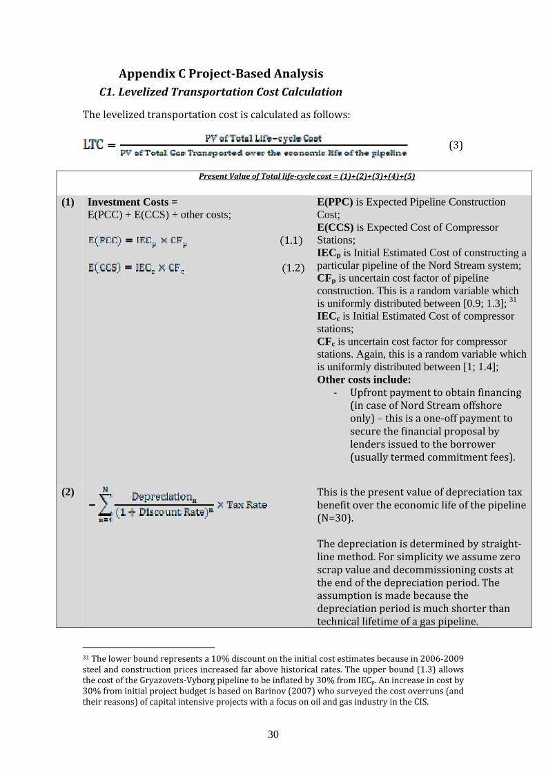
Appendix C ProjectBased Analysis C1. Levelized Transportation Cost Calculation
he levelized transportation cost is calculated as follows: T
(3)
Present Value of Total lifecycle cost = (1)+(2)+(3)+(4)+(5)
(1) Investment Costs = E(PCC) + E(CCS) + other costs;
1.1
1.2
E(PPC) is Expected Pipeline Construction Cost; E(CCS) is Expected Cost of Compressor Stations; IECp is Initial Estimated Cost of constructing a particular pipeline of the Nord Stream system; CFp is uncertain cost factor of pipeline construction. This is a random variable which is uniformly distributed between [0.9; 1.3]; 31 IECc is Initial Estimated Cost of compressor stations; CFc is uncertain cost factor for compressor stations. Again, this is a random variable which is uniformly distributed between [1; 1.4]; Other costs include:
‐ Upfront payment to obtain financing (in case of Nord Stream offshore only) – this is a one‐off payment to secure the financial proposal by lenders issued to the borrower (usually termed commitment fees).
(2)
This is the present value of depreciation tax benefit over the economic life of the pipeline (N=30). The depreciation is determined by straight‐line method. For simplicity we assume zero scrap value and decommissioning costs at the end of the depreciation period. The assumption is made because the depreciation period is much shorter than technical lifetime of a gas pipeline.
31 The lower bound represents a 10% discount on the initial cost estimates because in 2006‐2009 steel and construction prices increased far above historical rates. The upper bound (1.3) allows the cost of the Gryazovets‐Vyborg pipeline to be inflated by 30% from IECp. An increase in cost by 30% from initial project budget is based on Barinov (2007) who surveyed the cost overruns (and their reasons) of capital intensive projects with a focus on oil and gas industry in the CIS.
31
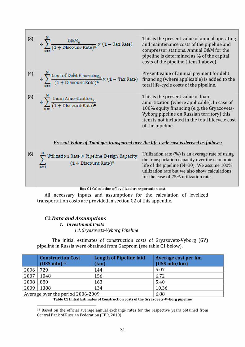
(3)
This is the present value of annual operating and maintenance costs of the pipeline and compressor stations. Annual O&M for the pipeline is determined as % of the capital costs of the pipeline (item 1 above).
(4) Present value of annual payment for debt financing (where applicable) is added to the total life‐cycle costs of the pipeline.
(5)
This is the present value of loan amortization (where applicable). In case of 100% equity financing (e.g. the Gryazovets‐Vyborg pipeline on Russian territory) this item is not included in the total lifecycle cost of the pipeline.
Present Value of Total gas transported over the life-cycle cost is derived as follows:
(6)
Utilization rate (%) is an average rate of using the transportation capacity over the economic life of the pipeline (N=30). We assume 100% utilization rate but we also show calculations for the case of 75% utilization rate.
Box C1 Calculation of levelized tr s
an portation cost
All necessary inputs and assumptions for the calculation of levelized transportation costs are provided in section C2 of this appendix.
C2. Data and Assumptions 1. Investment Costs
1.1. GryazovetsVyborg Pipeline
The initial estimates of construction costs of Gryazovets‐Vyborg (GV) pipeline in Russia were obtained from Gazprom (see table C1 below). Construction Cost (US$ mln)32
Length of Pipeline laid (km)
Average cost per km (US$ mln/km)
2006 729 144 5.07 2007 1048 156 6.72 2008 880 163 5.40 2009 1388 134 10.36 Average over the period 2006‐2009 6.88
Table C1 Initial Estimates of Construction costs of the GryazovetsVyborg pipeline
32 Based on the official average annual exchange rates for the respective years obtained from Central Bank of Russian Federation (CBR, 2010).

32
azarova (2010), Nazarova (20 prom (2005)
ates of
Source: Korchemkin (2010)
constru
, N 09), Gaz
Based on data from the table C1 we have derived the initial estimction costs of the Gryazovets‐Vyborg pipeline. During 2010‐2011,
Gazprom will have to finish laying down the rest of the Gryazovets‐Vyborg pipeline (320 km). Therefore, the expected cost of the Gryazovets‐Vyborg pipeline is estimated as follows.
(4)
The total cost of compressors to be installed along the Gryazovets‐Vyborg
ipelinp e was derived as follows. The Ukrainian producer of industrial equipments, Frunze, reported that it has produced four 25 MWh compressor units for installation at the beginning of the Gryazovets‐Vyborg pipeline (Frunze, 2010). The reported total cost of these compressors is US$52 mln (Ukrrudprom, 2010). Thus, if the total compressor power along the pipeline will be 1266 MWh, then the estimated cost of compressors to be equipped along the pipeline should be around US$ 660 mln. However, as was reported by Gazprom, the Portovaya Compressor station (366 MWh), which will compress gas before entering the Nord Stream offshore line, will be equipped with Rolls‐Royce’s compressor units with very advanced technology (52 MWh per compressor unit) (Gazprom, 2010c). It is thus reasonable to assume that 366 MWh of compressors purchased from Rolls‐Royce might cost Gazprom considerably more than those from the Ukrainian producer. We have factored this in as a cost overrun on purchasing compressors for the pipeline. Therefore, expected costs of the compressor stations along the Gryazovets‐Vyborg pipeline is calculated as:
(5)
1.2. Nord Stream Offshore
Initial estimates of construction costs of the Nord Stream offshore (NSO) is based on official figure of €7.4 bln, quoted by Nord Stream AG (NSAG) (Nord Stream AG, 2010a). However, as noted above there might be overruns or delays which would affect project costs.33 Major drivers of construction cost uncertainty include the uncertain costs of steel, construction, and engineering and procurement costs. The expected construction cost for the offshore pipeline is:
(6)
1.3. Opal, Nel and Gazelle Pipelines
33 Indeed recent news, quoting a representative of the Nord Stream pipeline, reported that the cost of the offshore pipeline could rise to €8.8 bln (Neftegaz, 2010).

33
The capital costs of Opal and Nel are quoted at €1 bln each (OPAL, 2010, NEL, 2010). For Gazelle project, the official figure for the capital cost is €400 mln (NET4GAS, 2010). As a starting point for the calculation of expected construction costs of these pipelines we use these official figures:
(7)
(8)
(9)
2. Financial Costs: and Interest Rates
2.1. GryazovetsVyborg Pipeline Discount
Since Gazprom is financing the construction of the Gryazovets‐Vyborg pipeline, the discount rate applied to the project is based on Gazprom’s weighted‐average cost of capital, WACC, in 2003‐2009 (see table C4). We treat WACC as a random variable which is uniformly distributed from [8.89; 15.41] with lower (upper) bound corresponding to the minimum (maximum) WACC in 2003‐2009. We apply an investment rule of WACC+1% for the discount rate of the Gryazovets‐Vyborg pipeline, following E.On’s rule for investments in new pipelines (Schenck, 2010).
2.2. Nord Stream Offshore (NSO)
‐
Debt Financing At the end of August 2009, Nord Stream’s offshore owner and operator,
NSAG, confirmed that Request for Proposals for the raising of senior debt for financing Phase 1 development have been issued to the commercial bank market.
According to NSAG, the construction of the offshore pipeline is to be financed with 30% equity from shareholders (Gazprom, BASF/Wintershall, E.ON Ruhrgas, Gasunie and GDF‐Suez) and 70% senior debt. As of mid March 2010, NSAG has completed the financial deal with commercial banking market on the financing of the first phase of construction. NSAG has procured the total debt requirement of approximately €3.9 bln for Phase 1 from a combination of the following (Mangham, 2009):
• A syndicated covered loan of up to €3.1 bln provided by a pool of 26 commercial banks. The loan is covered by Export Credit Guarantee Programmes of Germany (Hermes) and Italy (SACE) as well as the Untied Loan Guarantee Programme of Germany, UFK;
• A syndicated loan facility on an uncovered basis in an amount of up to € 800 mln.
The structure of the loan guarantee is as follows: – € 3.1 bln loan is a 16‐years loan facility covered by export credit
agencies Hermes, Sace, as well as by Germany’s loan guarantee programme UFK which covers political and commercial risk similar to Hermes. Hermes will cover €1.6 bln, UFK ‐ €1 bln and Sace ‐ €500 mln;
– There is also an €800 mln, 10‐year uncovered commercial loan. The pricing of the debts is as follows:

34
The €800 mln commercial uncovered loan pays a margin of 275 basis points (bps) over EURIBOR pre‐completion, 430 bps until year 7 and 450 bps thereafter. The commitment fee is 110 bps.
–
– The Hermes, UFK and Sace loans pay a margin of 160 bps, 180 bps and 165 bps over EURIBOR respectively. The commitment fees are 65 bps, 75 bps and 65 bps, respectively.
Based on these financial conditions, the interest rate on the debt finance is expressed as follows:
(10)
where c is the share of covered loan in the total debt finance, aj is the share of each export credit agency in total covered loan, pj is the price of each covered loan, aT is the share of total length of covered loan with a price pT, EURIBOR is the Euro interbank deposit rate.
As can be seen from financial conditions for phase I, the loan is the long‐term deal and the pricing of that loan is based on EURIBOR, which would need the trend of EURIBOR for 16 years in the future (the length of the covered loan). We assume that EURIBOR is a random variable with a distribution similar to its trend in 1999‐2009. This makes the EURIBOR trend in our cash‐flow model (2010‐2040) random.
‐
Equity Financing Since there are no details yet for the financial conditions of the second phase
of the Nord Stream offshore pipeline, we assume that the remaining investment costs are financed by NSAG shareholders. The cost of equity financing is discussed below.
‐
Project Discount Rate Taken into account the cost of debt financing and using the data on the cost of
capital for the investors (i.e., Gazprom, BASF/Wintershall, E.On Ruhrgas, Gasunie and GDF SUEZ) we have derived the WACC of the offshore pipeline which serves as the basis for the discount rate of the cash‐flow model. In its presentation of annual report 2009 (Bernotat, 2010), E.On reported that the company’s WACC during 2003‐2009 varied between 9% and 10% (see table C3). E.On also indicated that its investments in new‐build pipelines should exceed its WACC by at least 1%. Thus, we require the discount rate of the project to exceed the project WACC by 1%. Therefore, the project discount rate, DR, is derived as follows:34
(11)
34 We assume that WACC of the other two NSAG shareholders, Gasunie and GDF SUEZ, is similar to those of E.On and BASF since data on capital costs of Gasunie and GDF SUEZ was not publicly available. This assumption would not substantially undermine our results since both Gasunie and GDF SUEZ have relatively small shares in NSAG.

35
where dNSO – is the share of debt financing in the NSO project, ei ‐ share of shareholder in equity financing, WACC – is the cost of capital of each shareho
el
each lder i
respectiv y, ID – is weighted‐average interest rate on debt. The WACC of each investor in the project is assumed to be a random
variable which is uniformly distributed with minimum and maximum values specified in table C2.
Gazprom BASF E.On
Ruhrgas 2002 n/a n/a n/a 2003 8.98% n/a 10% 2004 9.03% n/a 9% 2005 8.91% n/a 9% 2006 9.13% 10% 9% 2007 11.32% 9% 9% 2008 15.07% 10% 9% 2009 15.41% 9% 9% Min 8.98% 9% 9% Max 15.41% 10% 10%
Table C2 WAC m lved m offshore pipeline
S er ), BA 0a)
2.3. elle
According t 09), Wingas has orrowed €500 mln to finance the Opal project. The interest rate, ID , on this loan is
Cs of Co
B
, N
panies invo in the Nord Strea
ource:
Opal
notat (2010
el and Gaz
SF (201
, BASF (2007)
o BASF’s annual report 2009 (BASF, 20b opal
2.5%. Ho ever, no nformation on the length of this loan has been provided. Thus, we assume that it is a short‐term loan (3 years) taking into account its relatively small size. We run sensitivity analysis on this assumption and found that a short‐term loan of 3 years will result in just a 7.8% increase in the levelized transportation cost compared to a longer‐term loan of 10 years. Thus, the assumption on the length of the loan contributes minimally to the cost calculations. The discount rate for the Opal project is derived as follows:
w i
(12)
where dopal is the share of debt financing, IDopal is the interest rate on the WAC is the cost of capital of Opal’s major investor (BASF and E.ON
loan, nd is Copal ), a
treated as a random variable with uniform distribution from [9%; 10%]. No public information is available on the details of financing the other two
pipelines, Nel and Gazelle. We assume that they are fully financed by project sponsors, i.e. Wingas and NET4GAS (former RWE Transgas Net, owned by RWE AG (RWE, 2010a)). We use BASF and E.ON WACC (see table C3) for the discount rate in cost calculations for the Nel project. For Gazelle project discount rate we use RWE’s WACC (9%‐10%) in 2002‐2009 (RWE, 2010b). The investment rule of WACC+1% is also applied here.
3. O&M Costs

36
Information on operating and maintenance (O&M) costs of pipelines is difficult to obtain because the considered pipelines are not yet in operation so we follow common practice in the literature and assume O&M costs to be a fixed fraction of investment costs of the pipeline (see e.g., ECT (2006); Krey and Minullin (2010)). We assume the annual cost of O&M of onshore pipelines to be 1.5% of their expected pipeline construction costs. For Nord Stream offshore pipeline, the O&M costs of the line are relatively lower than those of onshore pipes (Nord Stream AG, 2010b) so we assume O&M for offshore part to be 1% of the expected pipeline construction costs.
For O&M costs of compressor stations we use data from (Anders et al., 2006), who assume that each 1 horsepower (HP) used in a compressor station incurs $0.008 in O&M costs per hour of operation. For example, using a conve Hrsion factor 1341 P per MWh and assuming that compressors are used continuously (i.e., 8760 hours per annum), annual O&M costs of compressor stations for the Gryazovets‐Vyborg pipeline are:
e applied the same calculation for the Opal pipeline and the resultant O&M costs of compressor station is $8.5 mln per annum.
he information on compressor stations o
W
T f Gazelle and N pipeline were not p
el ublically available so we assumed that O&M costs of compressors would be
reflected in O&M costs of these pipelines. Sensitivity analysis on this assumption show as that if we factor in $8.5 mln of annu l O&M costs for a hypothetical compressor station (assuming a total power of 90 MWh, as in Opal pipeline, which would be too high for Gazelle as the distance is half the length of the Opal line), this would result in an increase of 4.7% on average in the total life‐cycle cost for Nel pipeline and 12.2% for Gazelle pipeline and consequently would increase the levelized transportation cost by 4.8% for Nel and 11.9% for Gazelle. Thus, a one per cent increase in total life‐cycle costs of the project gives around a one per cent increase in the levelized costs, which means a linear relationship between project costs and levelized costs. Thus excluding the O&M costs of compressor stations would not substantially affect our results.
4. Taxation and Depreciation
epreciation and taxation is based on the taxation system of the country through which the pipeline passes. For pipelines in Germany (Opal and Nel) the effective corporate tax rate, including trade tax and solidarity tax, is between 29‐32%
D
(CFE, 2010), so we assume a rate of 30%. For the Gazelle pipeline, according to KPMG, the relevant corporate tax in the Czech Republic in 2010 would be 19% (KPMG, 2009).
For the Nord Stream offshore pipeline, according to Nord Stream AG, the taxation issue would mainly be under Swiss jurisdiction as the company is registered in Kanton Zug with a headquarters of around 140 staff (Nord Stream AG, he a2010c). According to t tax system of Switzerland nd Kanton Zug (Müller‐Studer, 2009), Nord Stream AG enjoys special tax privileges because the company falls under the category of ‘mixed company’ i.e. a company whose main

37
operations are not in Switzerland35. This type of company has to pay Direct Federal Tax of 8.5% on total profit and 6.5% on 25% the total profit. This results in an effective corporate tax of 10.125% of total profit for Nord Stream AG.
35 At least 80% of operations should be outside Switzerland (Müller‐Studer, 2009).

38
Appendix D Transmission costs in Russia Following (The World Bank, 2009) we assume that at least transmission
costs for gas exports should be priced at LRMC of a new transmission pipeline. Since we have analyzed in details the new transmission pipeline Gryazovets‐Vyborg we apply its costs in calculation of transmission costs in Russia.
As noted above, Gazprom’s future gas production should come from existing fields (NPT) and increasingly from the Yamal Peninsula. We have calculated the distance from these two production regions to each entry point of Gazprom’s export routes (table D1).
TO
FROM Russia‐Ukraine border36
Russia‐Belarus border
Vyborg (Nord Stream route)
Production Region
Nadym‐Pur‐Taz37 2960 km 2850 km 3130 km Yamal Peninsula38 3330 km 2590 km 2870 km
Table D1 Distance between Gazprom’s production sites and export points
Source: Derived based on EIA (2010)
Since the pipeline costs are essentially linear in terms of distance over
similar terrain (ECT, 2006), the LRMC of gas transmission from production sites to each border point can then be derived as follows:
(13)where m and b are indices denoting the production region (NPT or Yamal) and border point (Russia‐Ukraine, Russia‐Belarus or Vyborg) respectively, LTCGV is the levelized transportation cost through the Gryazovets‐Vyborg pipeline, dGV is the len
gth of the Gryazovets‐Vyborg pipeline, dm,b is the distance between production sites and border points.
Following eq. (13) and using data from table D1, we calculated the pproximation of LRMC of gas transmission in Russia. The results are presented n taai ble D2.
TOFROM
RussiaUkraine border
RussiaBelarus border
Vyborg (Nord Stream route)
Production Region
Nadym‐Pur‐Taz (US$/tcm) 92.7 89.2 98.2 Yamal Peninsula (US$/tcm) 104.4 81.1 90.0
Table D2 Transportation cost within Russia
36 Gas metering station “Sudja” 37 Urengoi field was taken as representative of NPT production region 38 Bovanenkovo field was taken as representative of Yamal Peninsula production region
39
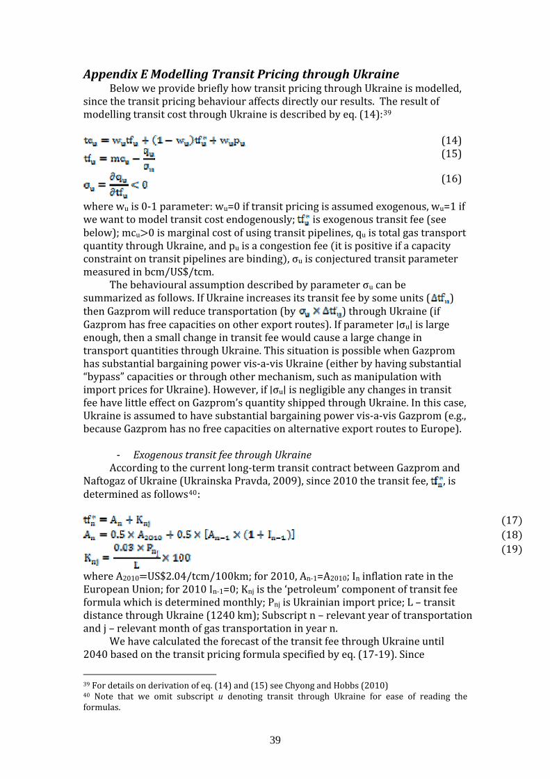
Appendix E Modelling Transit Pricing through Ukraine Below we provide briefly how transit pricing through Ukraine is modelled,
since the transit pricing behaviour affects directly our results. The result of modelling transit cost through Ukraine is described by eq. (14):39
(14)
(15)
where wu is 0‐1 parameter: wu=0 if transit pricing is assumed exogenous, wu=1 if we want to model transit cost endogenously;
(16)
is exogenous transit fee (see below); mcu 0 is marginal cost of using transit pipelines, qu is total gas transport quantity through Ukraine, and pu is a congestion fee it is positive if a capacity const parameter raint on transit pipelines are binding , σu is conjectured transit measured in bcm/US$/tcm.
The behavioural assumption described by parameter σu can be summarized as follows. If Ukraine increases its transit fee by some units ( ) then Gazprom will reduce transportation (by ) through Ukraine (if Gazprom has free capacities on other export routes). If parameter σu is large enough, then a small change in transit fee would cause a large change in transport quantities through Ukraine. This situation is possible when Gazprom has substantial bargaining power vis‐a‐vis Ukraine (either by having substantial “bypass” capacities or through other mechanism, such as manipulation with import prices for Ukraine). However, if σu is negligible any changes in transit fee have little effect on Gazprom’s quantity shipped through Ukraine. In this case, Ukraine is assumed to have substantial bargaining power vis‐a‐vis Gazprom (e.g., because Gazprom has no free capacities on alternative export routes to Europe).
‐ Exogenous transit fee through Ukraine
According to the current long‐term transit contract between Gazprom and aftogaz of Ukraine (Ukrainska Pravda, 2009), since 2010 the transit fee, N , is etermined as follows40: d
1718
where A2010 US$2.04/tcm/100km; for 2010, An‐1=A2010; In inflation rate in the European Union; for 2010 In‐1=0;
19
Knj is the ‘petroleum’ component of transit fee formula which is determined monthly; Pnj is Ukrainian import price; L – transit distan ation ce through Ukraine (1240 km); Subscript n – relevant year of transportand j – relevant month of gas transportation in year n.
We have calculated the forecast of the transit fee through Ukraine until 2040 based on the transit pricing formula specified by eq. (17‐19). Since
39 For details on derivation of eq. (14) and (15) see Chyong and Hobbs (2010) 40 Note that we omit subscript u denoting transit through Ukraine for ease of reading the formulas.

40
calculation of the transit fee requires forecasting the inflation rate, we have simulated possible future values of the inflation rate, taking its value as an uncertain variable with historical distribution of average inflation rate in 1997‐2009. The average value of the transit fee obtained from the simulations is US$25.6/tcm.41
41 The minimum value is US$25.5/tcm and the maximum value is US$25.8/tcm. This value does not include fuel cost to transport gas through Ukraine.