RESEARCH ARTICLE

The formulations of site-scale processes affect landscape-scale forest change predictions: a comparisonbetween LANDIS PRO and LANDIS-II forest landscapemodels

Jiangtao Xiao . Yu Liang . Hong S. He . Jonathan R. Thompson .

Wen J. Wang . Jacob S. Fraser . Zhiwei Wu

Received: 26 January 2016 / Accepted: 29 August 2016 / Published online: 6 September 2016

� Springer Science+Business Media Dordrecht 2016

Abstract

Context Forest landscapemodels (FLMs) are important

tools for simulating forest changes over broad spatial and

temporal scales. The ability of FLMs to accurately predict

forest changes may be significantly influenced by the

formulations of site-scale processes including seedling

establishment, tree growth, competition, and mortality.

Objective The objectives of this study were to

investigate the effects of site-scale processes and

interaction effects of site-scale processes and harvest

on landscape-scale forest change predictions.

Methods We compared the differences in species’

distribution (quantified by species’ percent area), total

aboveground biomass, and species’ biomass derived

from two FLMs: (1) a model that explicitly incorporates

stand density and size for each species age cohort

(LANDIS PRO), and (2) a model that explicitly tracks

biomass for each species age cohort (LANDIS-II with

biomass succession extension), which are variants from

the LANDIS FLM family with different formulations of

site-scale processes.

Results For early successional species, the differences

in simulated distribution and biomasswere small (mostly

less than 5 %). For mid- to late-successional species, the

differences in simulated distribution and biomass were

relatively large (10–30 %). The differences in species’

biomass predictions were generally larger than those for

species’ distribution predictions. Harvest mediated the

differences on landscape-scale predictions.

Conclusions The effects of site-scale processes on

landscape-scale forest change predictions are depen-

dent on species’ ecological traits such as shade

tolerance, seed dispersal, and growth rates.

Keywords Site-scale processes � LANDIS PRO �LANDIS-II � Species’ distribution � Species’ biomass �Harvest � Small Khingan Mountains

Introduction

Forest landscape dynamics are affected by site-scale

processes (e.g., establishment, growth, mortality, and

competition) and landscape-scales processes (such as

Electronic supplementary material The online version ofthis article (doi:10.1007/s10980-016-0442-2) contains supple-mentary material, which is available to authorized users.

J. Xiao � Y. Liang (&) � Z. Wu

Institute of Applied Ecology, Chinese Academy of

Sciences, Shenyang 110016, China

e-mail: liangysts@gmail.com

H. S. He � W. J. Wang � J. S. FraserSchool of Natural Resources, University of Missouri, 203

ABNR Bldg, Columbia, MO 65211, USA

H. S. He

School of Geographical Sciences, Northeast Normal

University, Changchun 130024, China

J. R. Thompson

Harvard Forest, Harvard University, 324 North Main St.,

Petersham, MA 01366, USA

123

Landscape Ecol (2017) 32:1347–1363

DOI 10.1007/s10980-016-0442-2

seed dispersal and disturbance) (Oliver and Larson

1996). Because the interactions of these multi-scale

processes are complex, forest landscape models

(FLMs) have emerged as valuable tools for predicting

forest dynamics over large spatial–temporal scales

(Keane et al. 2004; Perry and Enright 2006; Scheller

and Mladenoff 2007; He 2008; Taylor et al. 2009).

FLMs usually treat the simulated landscape as raster

cells (or sites). Site-scale processes are simulated in

each cell whereas forest landscape processes are

simulated across the study region. Because computa-

tion load increases with the complexity of site-scale

processes (e.g., more species or more detailed quan-

titative information), FLMs typically sacrifice the

realism of site-scale processes to make landscape-

scale simulation feasible (He 2008; Wang et al. 2013).

Recent FLMs attempt to improve simulation real-

ism with various designs to represent site-scale

dynamics, and these designs vary greatly (Lischke

et al. 2006; Scheller et al. 2007; Seidl et al. 2012;

Wang et al. 2013). For example, TreeMig (Lischke

et al. 2006) tracks horizontal and vertical stand

structure in a cell and accounts for seed production,

seed dispersal, seed bank dynamics, germination, and

sapling development. LANDCLIM (Schumacher et al.

2004) tracks numbers of trees and biomass by species’

age cohort; simulates the effects of abiotic factors

(terrain, soil, and climate) on tree size, density, and

biomass and simulates the resource competition-

caused mortality driven by maximum stand biomass.

LANDIS-II with its biomass succession module tracks

biomass by species’ age cohort and uses a ratio of

actual biomass to potential biomass to quantify

resource availability at each cell, assuming age-cohort

biomass by species incorporates stand density infor-

mation (Scheller et al. 2007, 2011). LANDIS PRO

(Wang et al. 2014a) tracks number of trees and

diameter at breast height (DBH) by species’ age

cohort; quantifies growing space using the stand

density index within each cell; and simulates resource

competition and stand development using theories of

stand dynamics.

Different formulations of site-scale processes in

FLMs may lead to differing simulation results (Elkin

et al. 2012; Liang et al. 2015). For example, species

relative abundance simulated by a FLM with detailed

site-scale processes based on stand density was

generally larger than that simulated by a model with

simplified site-scale processes (Liang et al. 2015).

Different tree growth formulations affected species

composition associated with elevation and species-

specific biomass (Elkin et al. 2012). Another study on

the effect of dynamic stand structure on succession

showed that using mean stand structures instead of

their horizontal and vertical distributions yielded

different transient and equilibrium species biomasses

(Loffler and Lischke 2001). FLMs long-term simula-

tions that did not explicitly include tree growth and

inter-species competition, resulted in long lived, shade

tolerant species (Schumacher et al. 2004). Some

studies also showed that FLMs with relatively simple

site-scale processes may have simulation results

similar to models with detailed site-scale processes,

because site-scale processes were frequently overrid-

den by landscape-scale processes in these landscapes

(e.g., clear-cut harvest or stand-replacing fire)

(Romme et al. 1998; Schumacher et al. 2004; Turner

2010). However, these simple FLMs may produce

biased predictions for forest landscapes where distur-

bance is infrequent and site-scale processes largely

drive forest landscape dynamics (Moorcroft et al.

2001; Schumacher et al. 2004; Elkin et al. 2012;Wang

et al. 2013).

Understanding the effects of site-scale processes is

important for reducing uncertainties in forest change

predictions. Despite many prior attempts, comparing

FLMs predictions remains challenging because dif-

ferences in FLM designs and formulation make it

difficult to identify and separate the effects of site-

scale processes. Comparing models with the same

modeling framework but different site-scale process

formulations can overcome some of these problems.

In this study, we evaluated two widely used FLMs,

variants from the LANDIS FLM family with different

formulations of site-scale processes, to investigate the

effects of site-scale processes on landscape-scale

forest change predictions: (1) a model that explicitly

incorporates stand density and size for trees of each

species by age cohort (LANDIS PRO), and (2) a model

that explicitly tracks biomass for each species age

cohort (LANDIS-II with biomass succession exten-

sion; but note that the biomass extension is one of

several available succession extensions for LANDIS-

II). Both LANDIS PRO and LANDIS-II models are

spatially explicit, raster-based landscape models,

which are used to simulate forest succession, seed

dispersal, wind, fire, biological disturbance, and

harvest over large spatial (e.g.,[106 ha) and temporal

1348 Landscape Ecol (2017) 32:1347–1363

123

(e.g., [102 years) scales with flexible spatial

(30–500 m pixel size) and temporal (1–10 years)

resolutions (Scheller and Mladenoff 2005; Gustafson

et al. 2010; Luo et al. 2014; Wang et al.

2015a, b, 2016). Specifically, we examined the

differences in species’ distribution (quantified by

species’ percent area), total aboveground biomass

(AGB), and species’ biomass between the two models

at the short-, medium-, and long-term, respectively.

We also investigated how landscape processes (har-

vest in this study) interacted with site-scale processes

and influenced landscape-scale predictions.

Methods

Case study landscape

Our study area (1.8 million ha) was located in Small

Khingan Mountains region of northeastern China

(Fig. 1). The topography is rolling with elevations

ranging from 139 to 1141 m. Climate is continental,

with long and cold winters (mean January temperature,

-1 �C) and short, but warm and humid summers (mean

July temperature, 21 �C). The annual precipitation

increases gradually from 485 mm in the north to

694 mm in the south. The area is dominated by brown

coniferous forest soils. The area is characterized as

mixed coniferous and broadleaved forests dominated by

Korean pine (Pinus koraiensis), spruce (Picea koraien-

sis and Picea jezoensis), fir (Abies nephrolepis), larch

(Larix gmelinii), oak (Quercus mongolica), elm (Ulmus

japonica), maple (Acer mono), ash (Fraxinus mand-

shurica), walnut (Juglans mandshurica), amur corktree

(Phellodendron amurense), ribbed birch (Betula cost-

ata), dahur birch (Betula davurica), basswood (Tilia

amurensis),white birch (Betula platyphylla), and poplar

(Populous davidiana). Because of extensive timber

harvest (clear-cut) in the 1970–1980s (Feng et al. 1999;

Bu et al. 2008), the age of early successional species

typically ranges from 30 to 40 years (even aged).

Model description

Both LANDIS PRO and LANDIS-II models stratify

heterogeneous landscapes into relatively homoge-

neous land types (also called ecoregions) based on

climate, soil, or terrain attributes (e.g., slope, aspect,

and elevation). Each land type is assigned unique

attributes, such as the probability that a species can

successfully become established in the absence of

competition (species establishment probability, SEP).

However, the fundamental difference in the philoso-

phy of these two models is that LANDIS PRO models

stand dynamics by density and size of species age

classes for each cell and then calculates biomass based

on allometric equations (e.g., Jenkins et al. 2004); In

contrast, LANDIS-II models total biomass production

for each cell and then partitions it into components by

species and age class (Scheller and Mladenoff 2004).

Because of the different designs in these two models,

site-scale information is tracked differently, which

results in different formulations of site-scale pro-

cesses, including establishment, tree growth, compe-

tition, and mortality.

LANDIS PRO

The LANDIS PRO model (http://landis.missouri.edu/

landispro70.php) explicitly simulates species-level

processes and inter- and intra-specific competition and

stand development by incorporating the number of trees

and DBH for each age cohort in each cell (Wang et al.Fig. 1 The geographic location of the study area

Landscape Ecol (2017) 32:1347–1363 1349

123

2013). Since stand parameters including species density

and basal area at each cell are compatible with forest

inventory data, LANDIS PRO can directly utilize forest

inventory data for model initialization, calibration, and

validation without a spin-up process, which allocates

initial biomass fromall the cohorts to specified age at the

start of the simulation (Wang et al. 2014b).

Growth

Tree growth is simulated as age and DBH increment

by species age cohort (Fig. 2). Age increment is

determined by the model time step. DBH increment is

achieved by species’ specific age-DBH relationship

customized for each land type (Murphy and Graney

1998; Loewenstein et al. 2000; Condit et al. 2006),

which can account for the effects of site quality on tree

growth. Generally, for shade-intolerant, early succes-

sional species, DBH reaches maximum at a faster rate,

whereas for shade-tolerant, mid- to late-successional

species, DBH increases at a slower rate.

Establishment

Seedling establishment is regulated by the seed disper-

sal, number of potential germination seeds per mature

tree (NPGS), proportionof total growing spaceoccupied

(GSO), species shade tolerance, and species establish-

ment probability. Seed dispersal is modeled as a

function of species effective and maximum seeding

distances (He and Mladenoff 1999). The number of

seeds reaching a cell is determined by NPGS and

dispersal distance. The total NPGS for each species is

accumulated from all available parent trees within the

dispersal kernel. For the seed estimated to arrive on the

cell, GSO is checked to determine whether there is

enough space for establishment. On an open growing

cell, the stand dynamics are characterized by extensive

seedlings establishment of various species except for the

most shade tolerant species, because that themost shade

tolerant species needs a relative shading environment to

establish and geminate. As the growing space is

gradually occupied (stand reaches crown closure), only

seedlings of shade tolerant species can establish

(Fig. 2). Once a seed is determined eligible, SEP as a

surrogate of environmental suitability is used to deter-

mine the probability for this seedling to become

established by comparing the species establishment

probability with a uniformly drawn random number

(0–1). This procedure captures the stochasticity of

species establishment and ensures that species with high

species establishment probability have higher probabil-

ities of establishment (Mladenoff and He 1999).

Competition

The competition intensity is regulated by the amount of

GSO within each cell. GSO is defined as the percentage

of the total physical growing space occupied by the trees

in each cell and is derived from Reineke’s stand density

index (Reineke 1933; Wang et al. 2013). Resource

availability varies among different stand development

stages because of the dynamics of establishment and

mortality. Four GSO govern progression through the

stages of stand development described by (Oliver and

Larson 1996; Wang et al. 2013). Seedlings can establish

depending on species’ shade tolerance and species

establishment probability at the stand initiation stage.

Once stands become fully occupied, competition-caused

mortality (self-thinning) is initiated, which follows

Yoda’s -3/2 self-thinning rule (Yoda et al. 1963). Self-

thinning continues to understory reinitiation and old-

growth stages if no disturbances occur (Wang et al.

2013).

Mortality

Tree mortality in LANDIS PRO includes: (1) stand-

scale resource competition-caused mortality (self-

thinning), (2) natural mortality due to reaching

longevity, (3) disturbance-caused mortality (Fig. 2).

Tree mortality due to self-thinning is characterized by

removing trees from small to large size classes and

from low to high shade tolerance classes. Thus, higher

shade tolerance species have lower mortality rates.

This form of mortality is tree-based as opposed to age

cohort-based (i.e., rather than modeling the death of an

entire age cohort as a single entity, individual trees or

subsets of trees within a cohort can die).

Harvest

In LANDIS PRO, the harvest module is developed

based on a previous LANDIS model (Gustafson et al.

cFig. 2 Comparison of LANDIS PRO succession and LANDIS-

II biomass succession

1350 Landscape Ecol (2017) 32:1347–1363

123

Landscape Ecol (2017) 32:1347–1363 1351

123

2000). However, because LANDIS PRO tracks den-

sity and basal area by species age cohort, its harvest

module can simulate basal area or stocking-level

controlled harvest actually used in forest management.

It can simulate most silvicultural treatments currently

used in forest management including single tree

selection, group selection, thinning from below,

thinning from above, and clear-cut (Fraser et al. 2013).

LANDIS-II

The LANDIS-II model (LANDIS-II 6.0 using the

Biomass Succession module http://www.landis-ii.org/

) represents each forest site in terms of aboveground

biomass by tree species age cohorts, rather than indi-

vidual trees (Scheller et al. 2007). The model was

developed as a framework to partition externally

estimated cell productivity—typically derived from a

physiologically-based lumped parameter model (e.g.,

PnET-II; Aber et al. 1995)—among species age

cohorts. AGB for each species at each time step is a

function of existing biomass, aboveground net pri-

mary productivity (ANPP), and mortality. In

LANDIS-II, initial biomass of each species age cohort

is calculated by ‘‘spin-up’’ all the cohorts to their

specified age at the start of the simulation (Scheller

and Mladenoff 2004; Scheller et al. 2007). For

example, if one species in a cell has two age-cohorts

(e.g., age 20 and 100), the 100-year cohort is modeled

to grow without competition for 80 years until the

20-year cohort is added. Then changes in the two

cohorts are projected forward for the remaining

20 years with competition between them for growing

space. A mortality fraction parameter specifies a

constant proportion of total cell biomass to be

removed at each time step. Thus, within the spin-up

phase, growth and mortality are simulated for the

number of years equal to each cohort’s current age,

and a cell’s initial biomass incorporates assumptions

about prior competition among existing cohorts.

Growth

Tree growth is simulated as both age and ANPP

increment by species age cohort (Fig. 2). This is done

through a species- and landtype-specific growth curve

parameter, which specifies ANPP as it approaches its

maximum (ANPPmax; Fig. 2). A cohort’s contribution

to ANPP increases with age (the ratio of actual cohort

biomass to maximum possible biomass for the cohort),

slowing asymptotically as total cell biomass approaches

Bmax.

Establishment

Seedling establishment in LANDIS-II is a function of

dispersal distance, species shade tolerance, onsite

biomass, and species establishment probability

(Fig. 2). The probability of seed dispersal is modeled

with two negative exponential probability distribu-

tions parameterized by the effective and maximum

seed dispersal distances of a species (Ward et al.

2005), which is based on a previous dispersal

algorithm (He andMladenoff 1999). Once seed arrives

at a given cell, light conditions are determined by

comparing the species shade tolerance and relative

living biomass (a percentage of actual biomass to

maximum cell biomass). Species with shade tolerance

classes 1–4 can only establish when the ratio is larger

than the user-defined percentages for each shade class

(1–4) (Scheller and Mladenoff 2004). Species in shade

tolerance class 5 (most tolerance) can establish under

any amount of living biomass. After checking light

condition, environmental suitability is checked by

comparing species establishment probability with a

0–1 random number. Seedlings established in

LANDIS-II are assigned a small amount of biomass

irrespective of seedling number and parent tree

abundance.

Competition

LANDIS-II simulates competition as a function of

Bmax, biomass already occupied by species age

cohorts and the growth rate specific to each species

as determined by the potential ANPP (ANPPpotential)

(Fig. 2). The actual ANPP for any species age cohort

is dependent upon ANPPpotential, cohort age, and

overstory competition. Competition reduces actual

cohort ANPP below its potential when canopy-dom-

inant cohorts suppress younger cohort and faster-

growing species outcompete slower-growing species.

Competition is expressed as measure of cohort

biomass compared to other biomass on the cell

(Scheller and Miranda 2015).

1352 Landscape Ecol (2017) 32:1347–1363

123

Mortality

LANDIS-II includes age-related mortality, competi-

tion-caused mortality, and disturbance-caused mortal-

ity (Fig. 2). Age-related mortality increases

nonlinearly with age, and a mortality curve parameter

determines how early in a cohort’s life span age-

related mortality begins. Competition-caused mortal-

ity increases also as a function of age, ANPPmax and

Bmax. Competition-caused mortality can remove

partial cohorts and is relatively low when a cohort is

young, accelerates to plateau as the cohort approaches

its longevity (Scheller and Miranda 2015).

Harvest

The harvest extension generally follows the previous

harvest module as described in Gustafson et al. (2000).

Stands are prioritized for harvest using user-defined

ranking algorithms (e.g., maximum cohort age) that

use biomass criteria related to forest management

objectives. For each harvest event, the number of cells

to be harvested must be indicated according to the

species and age cohort removal rules specified in a

prescription (e.g., clear-cut and thinning). Harvest can

remove all or a specified percentage of a cohort’s

biomass.

Model parameterization and calibration

LANDIS PRO and LANDIS-II shared two spatial data

inputs (land type map, forest composition map) and

other non-spatial parameters (e.g., species’ vital

attributes, species establishment probability). The

land type map in this study was derived from a digital

elevation model (DEM), which classified the study

area into 8 major land types. We modeled the most

prominent 15 tree species. The initial forest compo-

sition map at year 2000 including species and age

information was generated from forest stand inventory

data. Species’ vital attributes (Table 1) were estimated

based on previous studies and consultations with local

forestry experts (He et al. 2005; Yan and Shugart

2005; Bu et al. 2008). Species establishment proba-

bility for each species was estimated using a simula-

tion approach that used climate data and measures of

species climatic and edaphic tolerances (Gustafson

et al. 2010; Thompson et al. 2011). Besides the above

shared parameter, each model has its own specific

parameters.

Parameters specific to LANDIS PRO included

number of trees by species age cohort in each cell,

four GSO thresholds for each land type, and additional

species‘ vital attributes (e.g., growth rates, maximum

stand density index, NPGS, and maximum DBH). We

directly derived number of trees by species age cohort

at year 2000 from forest inventory data. Maximum

stand density index is defined as the maximum number

of 10-inch diameter trees per hectare, and has already

been reported for many species (Reineke 1933; Long

1985). We derived maximum stand density index and

DBH from literature and previous studies and growth

rates from forest inventory data (Burns and Honkala

1990; Liang et al. 2015). We iteratively calibrated the

growth rates and NPGS for each species using forest

inventory data and old-growth studies; for further

details on model calibration and evaluation see Wang

et al. (2014b). In addition, in order to test the

sensitivity of the growth rates and NPGS parameters,

we performed a sensitivity analysis for these two

parameters (see Appendix A in Supplementary

material).

Parameters specific to LANDIS-II included bio-

mass for each species age cohort at each cell,

ANPPmax by species, Bmax by species, foliar long-

evity and foliar lignin. We estimated ANPPmax from

PnET-II as the combination of wood and foliar NPP

and derived Bmax for each species from previous

studies (Feng et al. 1999; Luo et al. 2013). Additional

information about species vital attributes (e.g., foliar

longevity, foliar lignin) was based on Flora of China

(http://frps.eflora.cn/) or other literature (Li and Lei

2010). We calibrated the species’ growth and mor-

tality curve parameters using the approach described

in Scheller and Mladenoff (2004). In addition, in order

to test the sensitivity of the mortality and growth shape

parameters, we performed a sensitivity analysis for

these two parameters (see Appendix A in Supple-

mentary material).

Calibration for these two models was carried out by

comparing the shared output variables (such as

species’ biomass and total AGB). We initialized these

two models using forest inventory data from year

2000, ran each model to 2010, and compared the

simulated biomass at year 2010 with the 2010 forest

inventory data. We iteratively adjusted the species’

growth rates (age-DBH relationship) in LANDIS PRO

Landscape Ecol (2017) 32:1347–1363 1353

123

and the species’ growth and mortality curve param-

eters in LANDIS-II until biomass derived from each

model matched the summarized forest inventory data

from year 2000 at the landscape scale (pass Chi square

test for no differences in biomass).

Experimental design and data analysis

We simulated forest changes under two scenarios:

(a) succession only scenario, (b) succession and

harvest scenario (with harvest regime reflecting the

current harvest activities). We used both models to

simulate 15 dominant tree species (Table 1) from year

2000 to 2300 using 10-year time step at 100 m

resolution with five replicates to capture model

stochasticity. For each scenario the same forest

initialization was used.

We summarized the species’ distribution (quanti-

fied by species’ percent area), species’ biomass, and

total AGB by averaging simulation results from the

five replicate simulations for each scenario. We first

evaluated the differences in trajectories of species’

distribution and biomass, and total AGB between the

two models from year 2000 to 2300. We then assessed

the differences of species’ distribution and biomass

from the two models at short- (2000–2050

year), medium- (2060–2100 year), and long- (2110–

2300 year) term using the relative mean absolute error

(MAE %) (Miehle et al. 2006; Wang et al. 2014b):

MAE% ¼ 100Xn

i¼1Di � Pij j=n=D

where Di was the simulated result from LANDIS

PRO at year i, Pi was the simulated result from

LANDIS-II at year i, n (n = 5, 5, 20) is the number

of simulation years for each of short-, medium-, and

long-term, respectively. In order to avoid the same

percent area with different spatial patterns derived

from two models, we used cell-wise values to assess

the differences of species’ distribution. Furthermore,

we compared spatial patterns of species’ distribution

between these two models. All statistical analyses

were operated in the language and environment R

Team (2011). We found that six species (Korean

pine, spruce, oak, elm, basswood and white birch)

could capture the response patterns of 15 species,

thus we represented the simulations results of these

six species.Table

1Speciesparam

etersforvital

attributesin

theLANDIS

forest

landscapemodel

Genus

Species

LONGa

SMAa

STa

EDa

MDa

VPa

MIN

Sa

MAXSa

MaxDBHb

MaxSDIb

NPGSb

FLc

FLIc

Pinus

Korean

pine

300

40

450

150

00

0110

550

20

3.0

0.25

Picea

Spruce

300

30

450

150

00

090

600

20

4.0

0.25

Quercus

Oak

300

20

250

200

150

110

95

600

20

1.0

0.25

Ulm

us

Elm

250

20

3300

800

0.5

60

100

90

600

25

1.0

0.20

Tilia

Bassw

ood

300

30

350

200

0.8

30

110

85

650

20

1.0

0.20

Betula

Whitebirch

150

15

1200

2000

0.8

50

60

50

800

30

1.0

0.20

LONGspecieslongevity(years),SMAageofsexualmaturity

(years),STshadetolerance

class(1–5,1=

theleasttolerant,5=

themosttolerant),EDeffectiveseedlingdistance

(m),MDmaxim

um

seedlingdistance

(m),VPvegetativereproductionprobability(0–1),MINSminim

um

sproutingage(years),MAXSmaxim

um

sproutingage(years),MaxD

BH

maxim

um

diameter

atbreastheight(cm),MaxSDImaxim

um

standdensity

index

(number

of10-inch

treesper

ha),NPGSnumber

ofpotential

germinationseedsper

mature

tree

(number/cellarea),FLfoliar

longevity(years),FLIfoliar

lignin

(%ofmass)

aThesearetheshared

param

etersoftheLANDIS

PRO

7.0

andLANDIS-II6.0

withBiomassSuccessionextension

bThesearethespecificparam

etersoftheLANDIS

PRO

7.0

model

cThesearethespecificparam

etersoftheBiomassSuccessionextensionforLANDIS-II6.0

model

1354 Landscape Ecol (2017) 32:1347–1363

123

Results

Species’ distribution

The trajectories of distribution varied among species

and time and differed significantly between the two

models. The simulated percent area for white birch,

Korean pine and spruce from the models showed

similar trends across the 300 years’ simulation period

under the succession only scenario (Fig. 3). MAE %

averaged 2–10 % for these three species at the three

temporal terms (Fig. 4). The differences in trajectories

of percent area for oak, elm, and basswood between

the two models increased over time and were signif-

icant in the long-term (Fig. 3). For example, the

MAE % for oak, elm and basswood in the long-term

(14, 29, and 27 %) were larger than those in the short-

term (8, 15, and 7 %), respectively (Fig. 4). The

results of spatial pattern of species’ distribution were

consistent with results of species percent area. For

example, spatial pattern of distribution of oak simu-

lated by LANDIS PRO at year 2100 was larger than

that simulated by LANDIS-II, whereas for early

successional species (e.g., white birch), spatial pattern

of distribution was similar between these two models

at year 2100 (see Appendix B in Supplementary

material).

Total aboveground biomass (AGB)

The predictions of total AGB varied considerably

between the two models (Fig. 5). Total AGB simu-

lated by LANDIS PRO gradually increased and

peaked around simulation year 2200 (176 t/ha), and

then gradually decreased hereafter. Total AGB sim-

ulated by LANDIS-II increased more quickly to the

peak around the simulation year 2070 (178 t/ha)

followed by a 100-years’ stable fluctuations and

decreased dramatically to its lowest point (80 t/ha) at

the simulation year 2260. The results of MAE % for

total AGB were less than 10 % in the short- and

medium-term, whereas large in the long-term (22 %)

(Fig. 7).

The trajectories of total AGB under the harvest

scenario coincided basically with those under the

succession only scenario (Fig. 5). MAE % for total

AGB in the short-, medium-, and long-term (8, 8, and

13 %) under the harvest scenario were smaller than

those under the succession only scenario (9, 10, and

22 %) (Fig. 7).

Fig. 3 The trajectory of

species’ distribution

(quantified by species

percent area) simulated by

LANDIS PRO and

LANDIS-II across the

simulation period under

succession only scenario

Landscape Ecol (2017) 32:1347–1363 1355

123

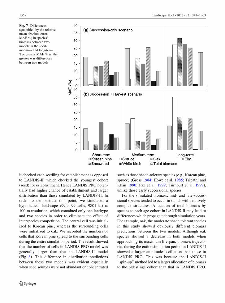
Species biomass

The trajectories of biomass between the two models

varied among species and time with generally increas-

ing differences over time. The trajectories of biomass

from the two models for white birch were similar

under the succession only scenario. MAE % averaged

5 % for white birch over time. Biomass for white birch

from both models increased in the short-term followed

by dramatic decreases in the medium-term, and

approximated zero in the long-term. The trajectories

of biomass for spruce, elm, and oak were similar in the

short- and medium-term but varied substantially in the

long-term under the succession only scenario. MAE

for spruce, elm, and oak were 28, 32, and 28 %,

respectively, in the long-term. The simulated biomass

for oak from LANDIS PRO gradually increased and

peaked around the simulated year 2230, and then

slowly decreased to year 2300. However, in LANDIS-

II, it increased much more quickly and peaked around

the simulated year 2180 followed by drastic decreases

under the succession only scenario (Fig. 6). The

trajectories of biomass for Korean pine and basswood

between both models had relatively stable differences

over time. MAE % averaged 20 % for Korean pine

and 21 % for basswood, which fell between white

birch and spruce, elm, and oak.

The trajectories of species’ biomass under the

harvest scenario coincided with those under the

succession only scenario (Fig. 6). Differences in

biomass for white birch were also smaller than those

for other species under the harvest scenario. Larger

differences of species’ biomass in the medium- and

long-term were observed under the harvest scenario

(Fig. 7). Harvest mediated the differences between the

twomodels (Figs. 6, 7). The differences in biomass for

most species from the two models under the harvest

scenario were smaller than those under the succession

only scenario (Fig. 7). For example, MAE % for

Korean pine, oak, and elm (16, 22, and 13 %) under

the harvest scenario were smaller than those under the

succession scenario in the long-term (20, 32, and

28 %). By contrast, spruce had an opposite situation.

MAE % for spruce in the short-, medium-, and long-

term (6, 21, and 35 %) under harvest scenario were

larger than those (1, 5, and 28 %) under the succession

only scenario (Fig. 7).

Fig. 4 Differences

(quantified by the relative

mean absolute error,

MAE %) in species’ percent

area between two models in

the short-, medium- and

long-term under succession

only scenario. The greater

MAE % were, the greater

the differences between two

models

Fig. 5 The trajectory of total aboveground biomass simulated

by LANDIS PRO and LANDIS-II across the simulation period

under succession only scenario and harvest scenario

1356 Landscape Ecol (2017) 32:1347–1363

123

Discussion

Our simulation results indicated that site-scale pro-

cesses such as tree growth, establishment, inter- and

intra-species competition, and mortality influenced

tree species’ distribution and biomass modeled with

FLMs. This is consistent with results from previous

studies on the effects of site-scale processes on

landscape-scale predictions using other forest land-

scape models (Elkin et al. 2012; Liang et al. 2015).

Moreover, the effects of site-scale processes on

landscape-scale predictions likely depend on species’

ecological traits.

For early successional species, the simulated dis-

tribution and biomass were more robust with respect to

different formulations of site-scale processes. For

example, trajectories of distribution for white birch

modelled with LANDIS PRO and LANDIS-II were

very similar. This is because early successional

species are usually fast growing, can better use

resources, and have high seed dispersal capacity.

These traits may potentially overcome low establish-

ment probabilities in less suitable areas (He and

Mladenoff 1999; Liang et al. 2015). Thus, distribution

predictions for these early successional species were

not sensitive to the formulation of site-scale processes.

In addition, early successional species tend to occur as

even aged stands in response to clear cutting

30–40 years ago in our study area (Feng et al. 1999;

Bu et al. 2008). Thus, biomass can be similarly

allocated to one age cohort in both models, which

eliminates the potential differences in allocating

biomass to multiple age cohorts. Moreover, the even

aged stands decreased simultaneously in simulated

distribution at the same time when they approach their

maximum lifespan. Since age-related mortality was

simulated similarly in both models, simulated biomass

for these species tends to be similar. Other observa-

tional studies also found no apparent effects of site-

scale processes such as seed mass on the growth and

distribution of early successional species (Dalling and

Hubbell 2002).

For mid- and late-successional species, simulated

distribution and biomass were sensitive to the formu-

lation of site-scale processes. Distribution was mostly

influenced by seed dispersal, which was simulated

differently in the two models. Both LANDIS PRO and

LANDIS-II used probability decay function in simu-

lating seed dispersal, i.e., the probability for an

arriving seed decreased with increasing seeding dis-

tance (He and Mladenoff 1999). However, since

LANDIS PRO tracked the number of arriving seeds,

Fig. 6 The trajectory of

species’ biomass simulated

by LANDIS PRO and

LANDIS-II across the

simulation period. Korean

pine and basswood had

higher biomass under the

harvest scenario in both

models than that under the

succession only scenario

because harvest of Korean

pine and basswood were

prohibited in China and

harvest of other species

promoted Korean pine and

basswood

Landscape Ecol (2017) 32:1347–1363 1357

123

it checked each seedling for establishment as opposed

to LANDIS-II, which checked the youngest cohort

(seed) for establishment. Hence LANDIS PRO poten-

tially had higher chance of establishment and larger

distribution than those simulated by LANDIS-II. In

order to demonstrate this point, we simulated a

hypothetical landscape (99 9 99 cells, 9801 ha) at

100 m resolution, which contained only one landtype

and two species in order to eliminate the effect of

interspecies competition. The central cell was initial-

ized to Korean pine, whereas the surrounding cells

were initialized to oak. We recorded the numbers of

cells that Korean pine spread to the surrounding cells

during the entire simulation period. The result showed

that the number of cells in LANDIS PRO model was

generally larger than that in LANDIS-II model

(Fig. 8). This difference in distribution predictions

between these two models was evident especially

when seed sources were not abundant or concentrated

such as those shade-tolerant species (e.g., Korean pine,

spruce) (Gross 1984; Howe et al. 1985; Tripathi and

Khan 1990; Paz et al. 1999; Turnbull et al. 1999),

unlike those early successional species.

For the simulated biomass, mid- and late-succes-

sional species tended to occur in stands with relatively

complex structures. Allocation of total biomass by

species to each age cohort in LANDIS-II may lead to

differences which propagate through simulation years.

For example, oak, the moderate shade tolerant species

in this study showed obviously different biomass

predictions between the two models. Although oak

species showed a decrease in both models when

approaching its maximum lifespan, biomass trajecto-

ries during the entire simulation period in LANDIS-II

showed a larger amplitude oscillation than those in

LANDIS PRO. This was because the LANDIS-II

‘‘spin-up’’ method led to a larger allocation of biomass

to the oldest age cohort than that in LANDIS PRO.

Fig. 7 Differences

(quantified by the relative

mean absolute error,

MAE %) in species’

biomass between two

models in the short-,

medium- and long-term.

The greater MAE % is, the

greater was differences

between two models

1358 Landscape Ecol (2017) 32:1347–1363

123

LANDIS-II does not use ecophysiology while simu-

lating biomass dynamics. It uses an empirical equation

to allocate biomass to cohorts. We randomly chose

approximately 4500 cells of oak stands with multiple

age cohorts from our study area to examine allocation

of biomass for the oldest age cohort at the simulated

year 2000, 2050, 2100, and 2200, respectively. The

result showed that the biomass of the oldest age cohort

in LANDIS-II was eight-fold larger than that in

LANDIS PRO at the simulated year 2000 (initial

year), whereas six-fold was found at the simulated

year 2100 (Fig. 9a). When a large portion of biomass

reached longevity and was removed, the rate of

mortality outpaced the rate of forest regrowth, making

LANDIS-II more sensitive to cohort senescence than

LANDIS PRO. This finding was magnified in our

simulations due to the lack of gap scale disturbance,

which may mediate the succession only effects (also

see discussion below).

As expected, prediction of total AGB was also

highly sensitive to the formulation of site-scale

processes, which stemmed from different mechanisms

determining biomass at the site scale. The maximum

in total AGB simulated by the two models was similar

(nearly 180 t/ha), which was supported by field-based

studies in this region (Hu et al. 2015). Total AGB

simulated by LANDIS-II increased much more

quickly to the maximum in the simulated short-term

and decreased dramatically to the minimum as cohort

senescence in the simulated long-term. By contrast,

predictions of total AGB showed less variation in

LANDIS PRO. In order to explain this phenomenon,

we analyzed species biomass increment (e.g., oak) by

time step (10 years) at various age cohorts (regener-

ation, early-stage, mid-stage, late-stage and old-

growth) simulated by these two models. The results

showed that biomass increments at late-stage and old-

growth in LANDIS-II were larger than those in

LANDIS PRO, whereas the increments at regenera-

tion, early-stage, mid-stage in LANDIS-II were

smaller (Fig. 9b). The more rapid increase of total

AGB in LANDIS-II than LANDIS PRO in the

simulated short-term resulted from a larger biomass

increment of age cohorts at late-stage in LANDIS-II

(the initial age of dominant mid- and late- successional

species typically range from 60 to 80 years). When a

large portion of biomass reached longevity and was

removed, the increase in regenerated biomass was

much less than the decrease in biomass caused by

mortality in LANDIS-II, making biomass decrease

dramatically. In contrast, the total AGB simulated in

LANDIS PRO decreased gradually after approaching

longevity due to the supplement in regenerated

biomass. This illustrates that LANDIS PRO, including

tree density, size, and seed number, and stand

development processes, can capture ecosystem inertia.

The differences in species’ biomass between the

two models were generally larger than those in

species’ distribution (Figs. 4, 7). This is probably

because biomass dynamics were mainly driven by

establishment, competition, and mortality, whereas

distribution change was mostly affected by establish-

ment and dispersal (Scheller et al. 2007; Xu et al.

2009; Wang et al. 2013, 2014a, b). Thus, site-scale

processes played greater roles in biomass dynamics

than in distribution, resulting in greater difference in

biomass between the two models. In addition, the

differences in predictions from the two models varied

over time. They were minimal in the short-term, but

increased from medium- to long-term.

We found that harvest mediated the effects of site-

scale processes on landscape-scale predictions, sug-

gesting that strong landscape-scale disturbance may

override site-scale processes. This may result from the

removal of mature trees. If a harvest removes the

mature trees, it will reduce the seed sources and make

the effects of seed dispersal less important. Thus,

differences in tracking seeds in LANDIS PRO and

LANDIS-II may lead to different results (Scheller and

Mladenof 2005). Harvest can also reduce competition

Fig. 8 We simulated a 9801 ha square landscape (99 9 99

cells) at a resolution of 1 ha containing only one landtype. The

central cell was initialized to Korean pine, the surrounding cells

were initialized to oak. The Y-axis represented how many cells

have Korean pine with seed dispersal across the simulation

period

Landscape Ecol (2017) 32:1347–1363 1359

123

and enable new species establishment especially for

less shade tolerant species; which further mediated the

effects of model results on site-scale processes. In

deciduous or mixed deciduous and coniferous forests

where large-scale disturbances (e.g., stand-replacing

fire and clear-cut) are infrequent, site-scale processes

are relatively more important than disturbances in

driving in forests dynamics (Wang et al. 2013).

Therefore, more detailed formations of site-scale

processes may be needed to improve the predictions

of forest changes in these regions.

The focus in this study was the effect of site-scale

processes on forest succession, gap scale disturbances,

such as windthrow, was not considered. This was

because methods used to simulate gap-scale distur-

bances differed in these two models, which made it

difficult to identify and separate the effects of site-

scale processes from wind disturbances. Under

scenarios with no windthrow disturbances, canopy

gaps were not frequent or sizable enough to allow

early successional species to establish. Thus, as

expected, these species almost disappear in the long

term. By contrast, stand heterogeneity would increase

if windthrow were simulated, which may result in

smaller differences between these two models.

Another limitation in this study was the impossibility

to parameterize the two models perfectly in parallel

despite our best efforts. This was because of the

differences in philosophy and methodology in the

modeling approaches. Consequently, different bio-

mass calculation metrics, allometric equations for

LANDIS PRO (Jenkins et al. 2004) and biomass

allocation in LANDIS-II (Scheller et al. 2007),

resulted in differences in simulated biomass.

The results about the effects of site-scale processes

on landscape-scale predictions could be generalized

Fig. 9 Biomass allocation

and annual biomass

increment of oak at various

age cohorts simulated by

LANDIS PRO and

LANDIS-II. About 15,000

cells in our study area had

oak stand age over 100 year

old age cohort, and 30 % of

which (approximately 4500

cells) were randomly chosen

to examine a allocation of

biomass at regeneration,

early-stage, mid-stage, late-

stage and old-growth,

simulated by LANDIS PRO

and LANDIS-II at the

simulation year 2000, 2050,

2100, and 2200 (PRO:

LANDIS PRO; II: LANDIS-

II); b the average biomass

increment of oak by time

step (10 years) at

regeneration, early-stage,

mid-stage, late-stage and

old-growth simulated by

these two models

1360 Landscape Ecol (2017) 32:1347–1363

123

and benefit other forest landscape modelling studies,

whereas the differences in seed dispersal and biomass

allocation, are relatively specific to these two models.

Although model-to-model comparisons as in this

study are meaningful and frequent in model evalua-

tion, it is necessary to apply long-term, landscape-

scale forest monitoring data to evaluate model

predictions. The comparisons between model results

and long-termmonitoring data were not feasible in this

study due to the insufficient long-term monitoring data

in the study area. With continuing efforts of forest

inventory, such data will eventually be available to aid

model comparison and evaluation. In addition, tem-

perate forests in the study area are influenced by global

change such as climate change. Climate change may

affect species establishment and mortality and alter

species’ distribution and biomass. Thus, model-to-

model comparisons under climate change scenario are

essential to evaluate model predictions, which is a next

desirable step.

Conclusion

Site-scale processes affected the tree species’ distri-

bution and biomass modeled with FLMs. The effects

of site-scale processes on landscape-scale predictions

likely depend on species’ ecological traits such as

shade tolerance, seed dispersal, and growth rates,

among other factors. For early successional species,

the simulated distribution and biomass were insensi-

tive to different formulations of site-scale processes.

Conversely, the simulated distribution and biomass for

mid- and late-successional species were sensitive to

the formulations. Moreover, the differences in the

simulated species biomass were generally larger than

in the simulated species’ distribution. In addition,

harvest mediated the effects of site-scale processes on

landscape-scale predictions, suggesting that strong

landscape-scale disturbance may override site-scale

processes. Results from this study revealed the agree-

ments and differences between these two models with

different site-scale process formulations. They may

help narrow down prediction uncertainties and point to

areas where representations of site-scale processes

need to be enhanced in the future.

Acknowledgments This research was funded by Chinese

National Science Foundational Project 31570461, 31300404

and 41371199 and University of Missouri GIS Mission

Enhancement Program. JT’s time was supported through NSF

LTER Grant No. NSF-DEB 12-37491.

References

Aber JD, Ollinger SV, Federer CA, Reich PB, Goulden ML,

Kicklighter DW, Melillo JM, Lathrop RG (1995) Predict-

ing the effects of climate change on water yield and forest

production in the northeastern United States. Climate Res

5(3):207–222

Bu R, He HS, Hu Y, Chang Y, Larsen DR (2008) Using the

LANDIS model to evaluate forest harvesting and planting

strategies under possible warming climates in Northeastern

China. For Ecol Manag 254(3):407–419

Burns RM, Honkala B (1990) Silvics of North America: 1.

Conifers; 2. Hardwoods. Agriculture Handbook 654,

USDA Forest Service, Washington, DC.

Condit R, Ashton P, Bunyavejchewin S, Dattaraja HS, Davies S,

Esufali S, Ewango C, Foster R, Gunatilleke I, Gunatilleke

C, Hall P, Harms K, Hart T, Hernandez C, Hubbell S, Itoh

A, Kiratiprayoon S, LaFrankie J, de Lao S, Makana J, Noor

M, Kassim AR, Russo S, Sukumar R, Samper C, Suresh

HS, Tan S, Thomas S, Valencia R, Vallejo M, Villa G,

Zillio T (2006) The importance of demographic niches to

tree diversity. Science 313(5783):98–101

Dalling JW, Hubbell SP (2002) Seed size, growth rate and gap

microsite conditions as determinants of recruitment suc-

cess for pioneer species. J Ecol 90(3):557–568

Elkin C, Reineking B, Bigler C, Bugmann H (2012) Do small-

grain processes matter for landscape scale questions?

Sensitivity of a forest landscape model to the formulation

of tree growth rate. Landscape Ecol 27(5):697–711

Feng Z, Wang X, Wu G (1999) Biomass and productivity of

forest ecoystems in China. Science Press, Beijing

Fraser JS, He HS, Shifley SR, Wang WJ, Thompson FR (2013)

Simulating stand-level harvest prescriptions across land-

scapes: LANDIS PRO harvest module design. Can J For

Res 43(10):972–978

Gross KL (1984) Effects of seed size and growth form on

seedling establishment of six monocarpic perennial plants.

J Ecol 72(2):369–387

Gustafson EJ, Shifley SR, Mladenoff DJ, Nimerfro KK, He HS

(2000) Spatial simulation of forest succession and timber

harvesting using LANDIS. Can J For Res 30(1):32–43

Gustafson EJ, Shvidenko AZ, Sturtevant BR, Scheller RM

(2010) Predicting global change effects on forest biomass

and composition in south-central Siberia. Ecol Appl

20(3):700–715

He HS (2008) Forest landscape models: Definitions, character-

ization, and classification. For Ecol Manag

254(3):484–498

He HS, Hao ZQ, Mladenoff DJ, Shao GF, Hu YM, Chang Y

(2005) Simulating forest ecosystem response to climate

warming incorporating spatial effects in north-eastern

China. J Biogeogr 32(12):2043–2056

He HS,Mladenoff DJ (1999) The effects of seed dispersal on the

simulation of long-term forest landscape change. Ecosys-

tems 2(4):308–319

Landscape Ecol (2017) 32:1347–1363 1361

123

Howe HF, Schupp EW, Westley LC (1985) Early consequences

of seed dispersal for a neotropical tree (Virola surina-

mensis). Ecology 66(3):781–791

Hu HQ, Luo BZ, Wei SJ, Wei SW, Sun L, Luo SS, Ma HB

(2015) Biomass carbon density and carbon sequestration

capacity in seven typical forest types of the Xiaoxing’an

Mountains, China. Chin J Plant Ecol 39:140–158

Jenkins JC, Chojnacky DC, Heath LS, Birdsey RA (2004)

Comprehensive database of diameter-based biomass

regressions for North American tree species. Gen. Tech.

Rep. NE-319. U.S. Department of Agriculture, Forest

Service, Northeastern Research Station, Newtown Square

Keane RE, Cary GJ, Davies ID et al (2004) A classification of

landscape fire succession models: spatial simulations of fire

and vegetation dynamics. Ecol Model 179(1):3–27

Li H, Lei Y (2010) Estimation and evaluation of forest biomass

carbon storage in China. China Forestry Press, Beijing

Liang Y, He HS, Wang WJ, Fraser JS, Wu Z, Xu J (2015) The

site-scale processes affect species distribution predictions

of forest landscape models. Ecol Model 300:89–101

Lischke H, Zimmermann NE, Bolliger J, Rickebusch S, Loffler

TJ (2006) TreeMig: A forest-landscape model for simu-

lating spatio-temporal patterns from stand to landscape

scale. Ecol Model 199(4):409–420

Loewenstein EF, Johnson PS, Garrett HE (2000) Age and

diameter structure of a managed uneven-aged oak forest.

Can J For Res 30(7):1060–1070

Loffler TJ, Lischke H (2001) Incorporation and influence of

variability in an aggregated forest model. Nat Resour

Model 14(1):103–137

Long JN (1985) A practical approach to density management.

For Chron 61(1):23–27

Luo X, He HS, Liang Y, Wang WJ, Wu Z, Fraser JS (2014)

Spatial simulation of the effect of fire and harvest on

aboveground tree biomass in boreal forests of Northeast

China. Landscape Ecol 29(7):1187–1200

Luo Y, Wang X, Zhang X, Lu F (2013) Biomass and Its Allo-

cation of Forest Ecosystems in China. China Forestry

Press, Beijing

Miehle P, Livesley SJ, Li C, Feikema PM, Adams MA, Arndt

SK (2006) Quantifying uncertainty from large-scale model

predictions of forest carbon dynamics. Glob Chang Biol

12(8):1421–1434

Mladenoff DJ, He HS (1999) Design and behaviour of LANDIS,

an object-oriented model of forest landscape disturbance

and succession. In: Mladenoff DJ, Baker WL (eds)

Advances in spatial modeling of forest landscape change:

approaches and applications. Cambridge University Press,

Cambridge, UK, pp 125–162

Moorcroft PR, Hurtt GC, Pacala SW (2001) A method for

scaling vegetation dynamics: the ecosystem demography

model(ED). Ecol Mono 71(4):557–586

Murphy PA, Graney DL (1998) Individual-tree basal area

growth, survival, and total height models for upland

hardwoods in the Boston Mountains of Arkansas. S J Appl

For 22(3):184–192

Oliver CD, Larson BC (1996) Forest Stand dynamics, Update

edn. Wiley, New York

Paz H, Mazer SJ, Martınez-Ramos M (1999) Seed mass, seed-

ling emergence, and environmental facts in seven rain

forest psychotria(Rubiaceae). Ecology 80(5):1594–1606

Perry GLW, Enright NJ (2006) Spatial modelling of vegetation

change in dynamic landscapes: a review of methods and

applications. Prog Phys Geogr 30(1):47–72

R Development Core Team (2011) R: a language and environ-

ment for statistical computing. R Development Core Team,

Vienna

Reineke LH (1933) Perfecting a stand-density index for even-

aged forest. J Agric Res 46:627–638

Romme WH, Everham EH, Frelich LE, Moritz MA, Sparks RE

(1998) Are large, infrequent disturbances qualitatively

different from small, frequent disturbances? Ecosystems

1(6):524–534

Scheller RM, Domingo JB, Sturtevant BR, Williams JS, Rudy

A, Gustafson EJ, Mladenoff DJ (2007) Design, develop-

ment, and application of LANDIS-II, a spatial landscape

simulation model with flexible temporal and spatial reso-

lution. Ecol Model 201(3–4):409–419

Scheller RM, Miranda B (2015) LANDIS-II Biomass Succes-

sion v3.2 Extension User Guide, p 5

Scheller RM, Mladenoff DJ (2004) A forest growth and biomass

module for a landscape simulation model, LANDIS: design,

validation, and application. Ecol Model 180(1):211–229

Scheller RM, Mladenoff DJ (2005) A spatially interactive

simulation of climate change, harvesting, wind, and tree

species migration and projected changes to forest compo-

sition and biomass in northern Wisconsin, USA. Glob

Chang Biol 11(2):307–321

Scheller RM, Mladenoff DJ (2007) An ecological classification

of forest landscape simulation models: tools and strategies

for understanding broad-scale forested ecosystems. Land-

scape Ecol 22(4):491–505

Scheller RM, Van Tuyl S, Clark K, Hom J, La Puma I (2011)

Carbon sequestration in the New Jersey pine barrens under

different scenarios of Fire management. Ecosystems

14(6):987–1004

Schumacher S, Bugmann H, Mladenoff DJ (2004) Improving

the formulation of tree growth and succession in a spatially

explicit landscape model. Ecol Model 180(1):175–194

Seidl R, Rammer W, Scheller RM, Spies TA (2012) An indi-

vidual-based process model to simulate landscape-scale

forest ecosystem dynamics. Ecol Model 231:87–100

Taylor AR, Chen HYH, VanDamme L (2009) A review of forest

succession models and their suitability for forest manage-

ment planning. For Sci 55(1):23–36

Thompson JR, Foster DR, Scheller RM, Kittredge D (2011) The

influence of land use and climate change on forest biomass

and composition in Massachusetts, USA. Ecol Appl

21:2425–2444

Tripathi RS, Khan ML (1990) Effects of seed weight and

microsite characteristics on germination and seedling fit-

ness in two species of Quercus in a subtropical wet hill

forest. Oikos 57(3):289–296

Turnbull LA, Rees M, Crawley MJ (1999) Seed mass and the

competition/colonization trade-off: a sowing experiment.

J Ecol 87(5):899–912

Turner MG (2010) Disturbance and landscape dynamics in a

changing world. Ecology 91(10):2833–2849

WangWJ, He HS, Fraser JS, Thompson FR, Shifley SR, Spetich

MA (2014a) LANDIS PRO: a landscape model that pre-

dicts forest composition and structure changes at regional

scales. Ecography 37:225–229

1362 Landscape Ecol (2017) 32:1347–1363

123

Wang WJ, He HS, Spetich MA, Shifley SR, Thompson FR,

Dijak WD, Wang Q (2014b) A framework for evaluating

forest landscape model predictions using empirical data

and knowledge. Environ Model Softw 62:230–239

Wang WJ, He HS, Spetich MA, Shifley SR, Thompson FR,

Larsen DR, Fraser JS, Yang J (2013) A large-scale forest

landscape model incorporating multi-scale processes and

utilizing forest inventory data. Ecosphere 4(9):106–117

Wang WJ, He HS, Thompson FR, Fraser JS (2016) Changes in

forest biomass and tree species distribution under climate

change in the Northeastern United States. Landscape Ecol.

doi:10.1007/s10980-016-0429-z

Wang WJ, He HS, Thompson FR, Fraser JS, Dijak WD (2015a)

Landscape- and regional-scale shifts in forest composition

under climate change in the Central Hardwood Region of

the United States. Landscape Ecol 31(1):149–163

Wang WJ, He HS, Thompson FR, Fraser JS, Hanberry BB,

Dijak WD (2015b) Importance of succession, harvest, and

climate change in determining future forest composition

changes in U.S. Central Hardwood Forests. Ecosphere

6(12):277

Ward BC, Mladenoff DJ, Scheller RM (2005) Landscape-level

effects of the interaction between residential development

and public forest management in northern Wisconsin,

USA. For Sci 51:616–632

Xu C, Gertner GZ, Scheller RM (2009) Uncertainties in the

response of a forest landscape to global climatic change.

Glob Chang Biol 15(1):116–131

Yan X, Shugart HH (2005) FAREAST: a forest gap model to

simulate dynamics and patterns of eastern Eurasian forests.

J Biogeogr 32(9):1641–1658

Yoda K, Kira T, Ogawa H, Hozumi K (1963) Self-thinning in

overcrowded pure stands under cultivated and natural

conditions. J Biol 14:107–129

Landscape Ecol (2017) 32:1347–1363 1363

123