WORKING PAPER NO. 13 August 2013

The Great Recession and the Two Dimensions of European Central Bank Credibility

Timo Henckel Gordon D. Menzies Daniel J. Zizzo

ISSN: 2200-6788 http://www.business.uts.edu.au/economics/

The Great Recession and the Two Dimensions of

European Central Bank Credibility∗

Timo Henckel

Centre for Applied Macroeconomic Analysis

Australian National University

Gordon D. Menzies†

University of Technology, Sydney &

Centre for Applied Macroeconomic Analysis

Daniel J. Zizzo

School of Economics and CBESS

University of East Anglia &

Centre for Applied Macroeconomic Analysis

August 20, 2013

Abstract

A puzzle from the Great Recession is an apparent mismatch between a fall in

the persistence of European inflation rates, and the increased variability of ex-

pert forecasts of inflation. We explain this puzzle and show how country specific

beliefs about inflation are still quite close to the European Central Bank target

of 2% (what we call official target credibility) but the degree of anchoring to this

target has gone down, implying an erosion of what we call anchoring credibility.

A decline in anchoring credibility can explain increased forecast variance indepen-

dently of any changes in inflation persistence, contrary to standard time series

models.

Keywords: central bank credibility, excess volatility, euro, inferential expec-

tations, inflation.

JEL Classification: C51, D84, E31, E52.

∗We thank Gianni Amisano, Christopher Carroll, Austin Gerig, Petra Gerlach, Tony Hall, JamesHansen, Adrian Pagan, Bruce Preston, Meghan Quinn, Julio Rotemberg, Pierre Siklos, Susan Thorp,

colleagues at CAMA (ANU) and seminar participants at the Australasian Macroeconomics Workshop

(Monash) 2012, for helpful advice, and Axel Sonntag for research assistance. The usual disclaimer

applies.†Corresponding author: University of Technology, Sydney, PO Box 123, Broadway NSW 2007,

Australia; gordon.menzies@uts.edu.au.

1 Introduction

Following the tumultuous events of 2008, inflation in the Euro zone has become less

persistent. In standard models of inflation, a reduction in persistence should coincide

with a reduction in the forecast error, but the reverse has been observed. This paper

is about how changes in central bank credibility can alter the forecast error variance of

inflation, independently of changes to its time series properties. We demonstrate that

this has in fact occurred in Europe in recent years.

For decades economists have studied the time series properties of inflation (Fuhrer,

2011). Early work assumed inflation was inertial, and the primary objective was to

accurately measure the degree of inertia by estimating inflation equations with several

higher-order lags (Gordon, 1982). Only later, with the advent of rational expectations

(RE), did researchers focus on the sources of this persistence. The first theoretical

RE models, which predicted very low or no persistence, failed to find support in the

inflation data. In order to add persistence to the RE models, it was necessary to in-

troduce structural frictions, such as nominal price contracting (Fischer, 1977, Taylor,

1980, Rotemberg, 1982, and Calvo, 1983). Models with frictions have been extensively

reworked (e.g. Dotsey et al., 1999; Mankiw and Reis, 2002) and still form the back-

bone of current monetary economics, including dynamic stochastic general equilibrium

(DSGE) models.

Empirically, there have been numerous attempts to explain changes in reduced-form

inflation persistence with reference to changes in the underlying determinants of infla-

tion. The most common explanation is a systematic change in monetary policy, since

it is well known that the coefficients of reduced form expressions are subject to insta-

bility from changing policies or beliefs (Friedman, 1968, and Lucas, 1972). Common

methodological approaches include tests for structural breaks in single-equation models

of inflation. As an alternative approach, Cogley et al. (2010) employ a time-varying

VAR to estimate the trend component of inflation.

In an important contribution, Benati (2008) notes that international evidence points

to a marked reduction in inflation persistence for countries that have adopted an official

inflation targeting regime.1 In the recent past, European inflation appears to have had

a fall in its persistence, measured by the coefficient on the lagged dependent variable

in a rolling 7-year annual regression of inflation on its lag.

(Insert Figure 1 about here)

Benati (2008) argues that the fall in inflation persistence for inflation targeting

countries is the consequence of well anchored expectations. In the limit, the central

bank’s commitment to the official inflation target is so strong that any deviation of

actual inflation from the target is assumed to be temporary and unplanned and therefore

unforecastable. Williams (2006) concurs, arguing that inflation in recent years may be

best described as the sum of a constant (the inflation target) and an i.i.d. error term.

1See also Darvas and Varga (2013) for central and Eastern European countries, Gamber et al.

(2013) for the US, and Siklos (2013a) for Asia-Pacific countries.

2

Following this line of reasoning, one might conclude from Figure 1 that inflationary

expectations in Europe have become more anchored in the recent past.

However, the results of Gerlach et al. (2011) pose a problem for this interpretation.

They find that professional forecasters since the Great Recession (GR) are less reliant on

past information, which is consistent with reduced aggregate autocorrelation implied by

Figure 1. But they also find that experts’ long term forecasts of inflation have become

more dispersed.

The difficulty here is that in many sensible time series representations of inflation

reduced persistence decreases the forecast error at any horizon, as well as the uncon-

ditional variance, the latter being an upper bound on the former.2 So the coexistence

of these two stylized facts (seemingly reduced variance based on declines in the persis-

tence of inflation and higher variance based on expert forecasting) is deeply puzzling.3

The puzzle–that there is a prediction of a correlation between these trends–would

disappear if, in fact, the two are not related.

Of course, one possibility is that the expert forecasts do not affect the actual inflation

process at all, in which case the dispersion of their forecasts is irrelevant. We eschew

this explanation, which we find implausible, and instead propose that the increased

variance of inflation forecasts could be explained by changes in beliefs about central

bank credibility.4 We model beliefs about central bank credibility by regarding the

central bank inflation target as a null belief in a hypothesis test (Henckel et al., 2011),

which can be modeled using the inferential expectations (IE) framework (Menzies and

Zizzo, 2009).

Within this framework we define two types of credibility. A central bank has official

target credibility if the null belief that agents hold corresponds to the official target

value. In the case of the ECB we will treat this value as 2%.5

The null belief could, however, take some other value. Anchoring credibility refers to

the capability of the central bank to anchor inflation to the value corresponding to the

null belief, whether or not this is the official target. Table 1 shows the two dimensions

of credibility.

2For = −1 + , the -step-ahead forecast error variance is 2¡1 + 2 + 4 + + 2(−1)

¢which is clearly increasing in . As approaches infinity, the expression asymptotes to the unconditional

variance 2¡1− 2

¢.

3We are grateful to Petra Gerlach for encouraging us to demonstrate this with a more general

structure (Appendix A).4As Pierre Siklos pointed out to us in private correspondence, there may be other reasons for

greater dispersion in inflation forecasts–e.g. forecasters’ heightened attentiveness since the GR; less

coordination among central bank forecasts; or greater central bank transparency (Siklos, 2013b).

For our empirical model the latter interpretation does not work, as transparency of the European

Central Bank (ECB) has not changed since the GR (Siklos, 2013a). The first two interpretations do not

necessarily contradict our proposition that a loss in central bank credibility leads to greater dispersion

in inflation forecasts. In particular, heightened attentiveness and less coordination among forecasters

most likely occur when the inflation rate moves away from its anchor, that is, precisely when central

bank credibility is compromised.5The European Central Bank (ECB) ‘aims at inflation rates of below, but close to, 2% over the

medium term’ http://www.ecb.int/mopo/html/index.en.html. In the absence of a meaning for ‘close’

we regard 2% as the target in our discussion. However, we return to this issue in the conclusion, and

show how one of our results is robust to changing 2% to what we will estimate the target to be for

Germany (1.65%). Apart from this one result, the ECB’s target is estimated econometrically in this

paper, rather than assumed, and so the particular value chosen is irrelevant.

3

Borrowing the usual nomenclature for statistical hypothesis tests, in Table 1 a high

means that an overwhelming majority of agents believe the null and a low means

that few do.6 Looking at the columns of Table 1, agents might believe that the ECB

is really targeting, say, 1%, in spite of its official pronouncements. That would be the

‘0 not at official target’ case which lacks official target credibility.

(Insert Table 1 about here)

We suspect that when most commentators refer to central bank credibility, or well

anchored expectations, they mean the top left corner of Table 1 where a high proportion

of agents believe the null, which, in turn, coincides with the official target (high and

0 at target). Fuhrer (2011) furnishes a good example:

“well-anchored inflation expectations require two things from the central

bank. First, the central bank must have an inflation goal [target] that is

known to the private agents in the economy, and second, the central bank

must move its policy rate in a way that systematically pushes the inflation

rate toward that goal.” (p. 474)

Fuhrer’s first requirement corresponds to our official target credibility, while his

second corresponds to our anchoring credibility. Yet he only considers well anchored

expectations to refer to a combination of the two when he refers to pushing inflation

‘towards that goal’ (our italics), rather than some other inflation target.7

We can agree with Fuhrer (2010) that when both requirements are met - the top

left corner of Table 1 - a central bank is credible; we can also say that, when both

requirements are not met - the bottom right corner of Table 1 -, a central bank is not

credible. As soon as we leave the left diagonal of Table 1, however, it becomes harder

to give a uni-dimensional designation ‘credible’ or ‘not credible’ to a central bank.

Suppose that the authorities accommodate a very high, even hyper-, rate of inflation

which can be accurately predicted (top right). We could describe this as the central

bank having anchoring credibility without official target credibility.8

For example, if experts during the Weimar Republic could predict inflation accu-

rately, the central bank would be credible on the former definition. The reader might

be uncomfortable using the word ‘credibility’ if the 0 belief is too far from a socially

desirable level, as it was in inter-war Germany, but this just strengthens our point that

it is conceptually useful to have a multi-dimensional description of credibility rather

than a binary choice along one dimension.

Naturally, it might be the case that in practice the two dimensions of credibility

are highly correlated, so that either is a sufficient statistic for the other. If this proves

to be the case, a single measure–a single dimension–will suffice for policymaking and

6In standard terminology, is the probabiliy of a type II error (falsely believing the null), and we

will show later that the null is indeed false in our model. With respect to the size of ’high’ and ’low’

in Table 1, we are not trying to define any particular thresholds. Table 1 is for heuristic purposes.7See also Demertzis et al. (2008).8The analytic content of Table 1 can be made even richer by giving content to the alternative beliefs

(1). We do so later.

4

other practical purposes. However, we will later present evidence that this is not the

case in Europe, suggesting the distinction between the two dimensions is as valuable in

practice as it is in theory.

The main result of this paper is that the European central bank still possesses a

good deal of official targeting credibility, but that the GR has led to a loss of anchoring

credibility.9 Our estimated equations will show that anchoring credibility loss is most

severe in Portugal, Ireland, Italy and Greece, which accords with our priors. In our

theoretical model, outlined in section 2, we assume that price setters rely on a consensus

(average) forecast by inflation experts (Carroll, 2003; Easaw and Golinelli, 2010) which

we model with IE. In section 3 we explain how the proportion of agents who believe the

target is related to the distribution of heterogeneous test sizes within the IE framework.

In section 4 we estimate inflation equations and confirm that the surveys of forecasters

in Gerlach et al. (2011) are consistent with an IE model of inflation. Section 5 justifies

our approach by showing that the two measures of credibility are relatively uncorrelated,

and concludes.

2 IE in the Country Specific Phillips Curve

The theoretical building block is an augmented Lucas supply function of the form,

= + 1 + 2 1 2 0 (1)

where denotes actual inflation in period , expected inflation, and real marginal

cost. We augment the equation for the mechanical impact on inflation of energy prices

, which is important empirically for Europe. We are not interested in the determi-

nants of in general equilibrium. We therefore assume that has a zero mean but we

leave unspecified whether it is autocorrelated. It is straightforward to use a mapping

of real marginal cost to output or unemployment to rewrite (1) so that becomes

an output gap. An example of a derivation of the supply function (1) is provided in

Appendix B.

Expected inflation need not be the mathematical expectation. In particular,

it may represent the average of a range of heterogeneous expectations, as in our case

below. There is no forward-looking inflation expectation term, as in the New Keynesian

Phillips curve, because prices are assumed to be perfectly flexible, providing firms with

the opportunity to set prices anew in each period.

The coefficient 2 of real marginal cost may reflect institutional features or the

relative weight attached to a noisy signal of as in a standard signal extraction problem.

In our model expected inflation is assumed, in the spirit of Carroll (2003), to be

the consensus belief of experts about the true inflation target of the central bank, .

In particular, we assume that in each Eurozone country a continuum of experts, after

studying the economy and the central bank, separately guess . These within-country

guesses are averaged and form a consensus belief which substitutes for in the first

term on the RHS of (1) in each country’s Phillips curve.

9Using different approaches, Galati et al. (2011) also conclude that inflation expectations in the

Euro area have become less firmly anchored during the crisis while Albinowski et al. (2013) argue that

trust in the ECB has suffered in this period.

5

We assume that experts have inferential expectations (IE), that is, they guess

using a statistical hypothesis test. We further assume that all expert groups in each

Eurozone country use the same p-value of a test statistic as they guess . We

consider this a reasonable approximation as a common ECB monetary policy implies

similar information sets. That said, we assume that each individual expert in a country

group of experts has her own significance level . Thus, heterogeneity is located in the

diverse extent of belief anchoring in each country group.

In many circumstances it might be natural to assume that the IE test statistic of

a central bank is some function of the departure of inflation from the target (here,

the 2% ECB target). For example, this was the assumption of Henckel et al. (2011).

However, in the current crisis, it is both realistic and convenient to assume that the

danger to credibility does not stem from the recent inflation history. It is realistic

because inflationary concerns relate to the doubts about the fiscal sustainability of the

Euro venture itself (Borgy et al., 2011),10 and it is convenient because the independence

of and lagged inflation makes our estimation below simpler.11

There would be no inference problem for the experts in the model described in (1)

if were common knowledge and credible. However, it is possible for the central

bank to lie about–or anyway not follow through coherently with–monetary policy, in

the sense of genuinely targeting a value of inflation different from the official value.12

Using the notion of official target credibility, as previously defined, we denote ∗ theannounced inflation target which may or may not equal . To the extent that agents

believe differs from ∗, official target credibility is eroded.In the IE framework it is a standard discipline to adopt rational expectations as the

alternative hypothesis (Menzies and Zizzo, 2009; Henckel et al., 2011).13 Adopting that

convention here suggests the following hypotheses:

0 : = ∗

1 : = []

where [·] is the mathematical expectation operator. That is, the null hypothesis isthat the central bank is really pursuing its announced target, but when experts do not

believe that, they embrace RE.

We assume that all the experts combine their beliefs about inflation together, and

their weighted average determines price setters’ beliefs, with a proportion of experts

believing 0 and a proportion (1− ) believing 1. Substituting into (1) and allowing

for an i.i.d. estimation error, , we obtain:

= ∗ + (1− ) [] + 1 + 2 + (2)

10We do not need to assume this however - inflationary concerns could be due to a range of eco-

nomic factors and, as long they do include recent inflation history, this would be compatible with our

framework.11The dependence between the proportion of agents holding onto beliefs and lagged values of the de-

pendent variable make the chartists/fundamentalists framework (Ahrens and Reitz, 2000, and Frankel

and Froot, 1986) very challenging to estimate. Our assumption is a reasonable shortcut for this par-

ticular context which makes estimation straightforward.12Alternatively, an inflation bias may be present, implying a wedge between the official inflation

target and the actual equilibrium value, and this is imperfectly observed by experts. This latter

possibility is in the spirit of Barro and Gordon (1983a, 1983b) and Henckel et al. (2011).13This has the considerable advantages of model parsimony and of nesting RE as a special case of

IE, for when = 1 the null must be rejected and RE obtains.

6

Agents who have rational expectations know the model and calculate the rational

expectation of inflation based on (2). We can take mathematical expectations through

(2), solve for [], and then substitute back into (2) to obtain the IE Phillips curve.14

Solving for the expectation of (2) and substituting it back into (2) yields

= ∗ +1 +

2 + (3)

Equation (2) shows how inflation is affected directly by ∗, and and indirectly bybeliefs about these variables embedded in []. Let = 1

+ 2 and substitute

the expectation of (2) back into (2):

= ∗ + (1− ) [] + +

= ∗ + (1− ) ( [∗] + (1− ) [ []] + []) + +

= {∗ + (1− ) [∗]}+ { + (1− ) []}+ (1− )2 [ []] +

Define the expectations operator such that [ [·]] = 2 [·]. Repeated substitutionof the expectation of (2) into [], 1, demonstrates, upon rearranging, that

inflation depends upon beliefs about beliefs, viz. higher-order beliefs:

= ©∗ + (1− ) [∗] + (1− )

22 [∗]

ª+© + (1− ) [] + (1− )

22 []

ª+ (1− )

33 [] +

making substitution times

= n∗ + (1− ) [∗] + + (1− )

[∗]

o+n + (1− ) [] + + (1− )

[]

o+ (1− )

+1+1 [] +

Appealing to the law of iterated expectations ( = ) and conditioning on and ∗,

we have that [] = and [∗] = ∗ and thus,

= n∗ + (1− )∗ + + (1− )

∗o

+n + (1− ) + + (1− )

o+ (1− )

+1+1 [] +

When goes to infinity we see that the impact on inflation of beliefs about beliefs

concerning compounds, since inflation is driven by the sum of a geometric progres-

sion¡1 + (1− ) + (1− )

2+

¢ = when 1. In contrast, the impact on

inflation of beliefs about beliefs concerning ∗ cancels out, since the geometric progres-sion

¡1 + (1− ) + (1− )

2+

¢∗ = ∗ is pre-multiplied by , and the ’s cancel.

Writing out the relevant geometric progressions gives us an alternative expression for

(3), which makes it clear why there is a unitary marginal impact of ∗ on and an

14The pronumeral ∗ could be anything that can be conditioned on at time , including an autore-gression in . We assume ∗ is the official inflation target since that is the normal anchor in an inflationtargeting regime.

7

impact of which grows as decreases:

= lim→∞

³n∗ + (1− )∗ + + (1− )

∗o

+n + (1− ) + + (1− )

o+ (1− )

+1+1 []

´= (∗ + )

¡1 + (1− ) + (1− )

2+

¢+ 0

= (∗ + )| {z }direct

+1−

(∗ + )| {z }

beliefs about beliefs

(4)

Intuitively, when is unity, all agents believe the inflation target, but inflation itself

is buffeted about by mechanical forces which are represented by . This can be seen

by direct substitution of = 1 into (2), or by noting that there is no impact of beliefs

about beliefs in the second term of the last line of (4).

When = 0, direct substitution into (2) fails.15 However, we can take the limit of

(4) as goes to zero. A story emerges where agents who abandon 0 recognize that

some other agents still believe it, so the agents who have rejected 0 still have to factor

∗ into their (rational) expectation.If approaches zero there is a very strong effect of beliefs about beliefs in (4),

because (1− ) is close to unity, and so even if a vanishingly small group of agents

anchor onto 0, the effect of beliefs of agents who believe 1 about the 0 agents’

beliefs offsets this, and ∗ appears in the Phillips curve with a unit coefficient. Incontrast, the effect of beliefs about beliefs concerning grows, because the increasing

proportion of agents who believe 1 have to take into account the mechanical effects on

inflation of in the beliefs about beliefs of other rational agents, and so the marginal

impact of grows with (1− ) in the IE Phillips curve.

To flag the most germane insight of this section, if (3) is used to forecast inflation,

a lower share of agents anchoring onto the null (i.e. a low ) leads to a higher forecast

error variance in the future, for a given variance of energy prices and output gaps. This

explains how forecast errors can be buffeted about by central bank anchoring credibility,

irrespective of persistence, which is the main point of the paper.

A final comment on (3) is that inflation differs from its rational expectation ( [])

by a white noise error . That is, although the whole model cannot be called a rational

expectations model, since some agents default to the null if is non-zero, inflation

expectations themselves are model consistent and therefore rational. Two things follow

directly from this.

First, the true state of the world (at least up to a white noise error) is that the null

is false so is actually the probability of a type II error, in line with standard statistical

terminology, as flagged earlier.

Second, standard evolutionary arguments for convergence to rational expectations

could be made (Alchian, 1950). The validity of our model would then depend upon some

implicit calculation costs, inattention, or belief inertia borne of psychological factors.16

15After making the substitution, a contradiction ensues if expectations of the resultant equation are

taken.16For a discussion of anchoring driven by belief conservatism see Lyons et al. (2012) or Edwards

(1968). For a discussion of attention due to other factors expending the cognitive resources of agents

8

3 and

In this section we demonstrate how changes in beta relate to changes in anchoring

credibility (that is, the tendency of agents to believe 0). Readers who are prepared

to accept that an increase in the proportion of agents who believe 0, for a given ,

corresponds to an increase in belief conservatism may wish to jump straight to section

4.

The conceptual challenge is that with heterogeneity across ’s we cannot explain a

change in by a change in a single representative agent’s , which is the off-the-shelf

measure of belief conservatism in IE. If falls by, say, 20%, does that mean that the

whole distribution of ’s is ‘more conservative’ in some sense? Answering questions like

these require that we map changes in onto changes in the shape of an distribution.

To do this, we need to find a way to describe whole distributions as being more, or

less, belief conservative. To that end, we first outline the relationship between and

the distribution of . In any hypothesis, 0 is maintained if a p-value ( ) fails to fall

below the test size, that is if . This immediately gives us :

=

Z

0

= ( )− (0) (5)

Can we now limit the set of densities such that an increase in implies more

conservatism for any ? To be concrete, imagine several groups of experts, one for

each country in the Eurozone. Thus, there is a group in the Netherlands, a group in

Spain, and so on. We conceive of each individual expert in, say, Spain, drawing from

a Spanish distribution of test sizes. In what sense can a Spanish distribution of ’s

become more belief conservative?

Intuitively, if a group of Spanish experts has a distribution of with an increasing

probability mass around zero, we could describe the group as becoming more ‘conserv-

ative’ in the sense that a randomly chosen is likely to be closer to zero. But it is not

hard to create cases where some probability mass shifts towards zero, and some shifts

towards unity.

So, to pin down a clear taxonomy, we confine our attention to a change in the

distribution which is uniformly more conservative. This is a switch to an density

that delivers a higher value of the integral in (5) compared to an original density

for any value of : Z

0

Z

0

∀ ∈ (0 1) (6)

This, then, is our way of mapping onto the shape of an distribution. If Spanish

, say, increases and we assume is unchanged, then we can say that it is as if the

Spanish distribution of has become uniformly more conservative.

see Andrade and Le Bihan (2010) and Luo and Young (2010), which relate to earlier papers (Reis,

2006; Sims, 2003; Mankiw and Reis, 2002). Another justification for IE based on the supposed logical

consistency of economists is that it removes what we might call ‘expectational asymmetry’. If we,

as economists, use hypothesis tests in helping form our beliefs, then we should also expect agents in

our models to do so. This is redolent of the Public Choice revolution which removed ‘motivational

asymmetry’ from the analysis of government. It will be recalled that these scholars asked why the

governed were assumed to be self interested while the government was benevolent.

9

Confining our attention to uniformly more conservative distributions means that

we can make a claim about changed conservatism even if we do not know what is.

That is, if we are examining a cross section of country expert groups under the same

monetary regime, then all we need to do is assume they have the same , even if we do

not know what it is. If we observe estimated ’s change differentially across European

economies, as we do in the next section, we can attribute the differential changes to

changes in belief conservatism.17

We conclude this section by illustrating the simplest possible example of a uniformly

more conservative distribution, and leaving more general pdfs to Appendix C. The

simplest distribution is a straight line density, that is where 0 () is a constant. Theproperties of pdf’s allow us to derive an explicit formula:

0 () =

=

∴ = + and

Z 1

0

= 1 ⇒ = 1−

2

∴ = + 1−

2

If there are conditions under which will rise for any value of , then according to

(6) those conditions will define a change in that is uniformly more conservative:

=

Z

0

µ+ 1−

2

¶ (7)

=

Z

0

µ+ 1−

2

¶ =

Z

0

µ−

2

¶ =

− (1− )

2 0

So, for any , if decreases, increases. Thus, a decrease in makes more

uniformly conservative. Graphically, a decrease in shifts the probability mass towards

zero everywhere on the distribution.

The analysis in this section allows us to connect increases in estimated to uni-

formly more conservative shifts in the distribution of . Since these explanations are

not dependent on the particular value of , we will be able to infer changes in the

distribution of in different countries when everyone has a common, but unknown, .

Naturally, this only applies as we look across countries at a point in time. Through

time, ’s may change as the evidence against the null changes, but if that alone is the

cause it will do so equally across all countries by assumption. Differential responses

through time will indicate changes in belief conservatism across countries.

17This may be controversial since it is more natural to speak of the (singular) credibility of the

single monetary authority, the ECB. We, however, speak of credibility in individual Eurozone countries

meaning credibility as perceived by price setters within each country. As explained in the text this

enables us to cleanly identify changes in cross-country belief conservatism while keeping monetary

policy, and information about monetary policy, common across all countries. Another justification

is that the Euro has been sufficiently imperiled by recent events that there is a ‘shadow’ central

bank–with its own credibility–sitting within each country waiting to be (re)born, should the country

concerned abandon the Euro. We take our later results, which identify a differential erosion of anchoring

credibility in Portugal, Ireland, Italy and Greece, as providing support for our approach.

10

4 Estimates of Credibility

4.1 An Estimable Form of the Model

Equation (3) is the basis for our estimation. To obtain a measure of official target

credibility we also allow the steady state inflation rate to change after the crisis (that

is, from the September quarter of 2008). We estimate the following over March 2001

until December 2012:18

= 1 (1−) + 2 +3

1− 5 +

4

1− 5 + (8)

The parameters 3 and 4 in (8) equal 1 and 2 in (3) prior to the crisis, while

3 (1− 5) and 4 (1− 5) are the post crisis parameter ratios, after has fallen by

a proportion 5. They represent the impact of the energy price and the output gap on

inflation, which operates both directly, and indirectly via expectations. The parameter

5 should have an absolute value of no more than unity.19 The proportional reduction

applies equally to both coefficients, which is what is implied by (3). Inflation () and

energy price growth relative to trend () are both four-quarter ended.20 The dummy

takes on unity from September 2008, and the output gap is the deviation of the log

of GDP from an OLS trend.21 The parameters 1 and 2 are the pre- and post-recession

inflation targets as perceived by experts.

The raw estimates are shown in Table 2. In 2A, we show both the Euro area model,

where we assume a single group of experts over the whole Euro area and we use an

aggregate price index and output gap, and countries with a high estimate of 5. In

Table 2B, we have the remaining countries with lower values of 5. The models for

Netherlands and Finland have a low adjusted 2, whereas the others have adjusted 2

values around or above 05.

(Insert Table 2 about here)

With the exception of 5 for Ireland, which exceeds unity though not statistically

significantly so (two-tailed = 0117), all other coefficients are within economically

18The estimation period is partly dictated by measurement issues in the output gap (described in

a subsequent footnote) and partly by Greece’s delayed entry into the Euro in 2001. We can interpret

1 and 2 as steady state inflation because we transformed the data for energy price inflation to be

deviations from trend, which is zero in the steady state.19Of course it could be negative, implying a rising . The denominators are set up with minus

signs only because we knew that was falling from exploratory regressions, but this is without loss of

generality.20Four-quarter-ended energy CPI is subtracted from the mean over March 2001-December 2012.21Data was collected from 1998, and four-quarter ended price changes therefore began in 1999. Initial

attempts to map annual output gap data from the OECD to quarterly OLS residuals of log output onto

a linear trend from 1998 onwards ran into serious difficulties when the OLS residuals over 1998-2000

showed large negative gaps in Austria, France, Ireland, Italy, Luxembourg and the Netherlands, while

the OECD ones showed positive or only marginally negative ones. In the end we used OLS residuals

from 2001 based on a regression of log output on trend over the whole period, namely 1998-2012. These

matched the OECD annual figures well over this truncated period.

11

reasonable ranges. The estimated inflation targets are all below 5% and many are close

to the ECB’s 2% target. All of the statistically significant coefficients on energy price

inflation, 3, are in the 0.05 to 0.10 range, which is not implausible considering energy

has a weight of around 10 per cent in the CPI of European countries.22 The only

significant output gap term, for Germany, has an estimated coefficient of 0.2, which is

also reasonable.

We set about simplifying the models in a number of ways. First, we deleted a number

of insignificant coefficients. The Euro area equation was left untouched. Although the

output gap was technically insignificant, the p-value was 0.1044, and the estimated

effects before and after the recession (0.04 and 0.09) seemed economically reasonable.

We also refrained from deleting 3 and 4 for Italy and Greece. Although the coefficients

are insignificant, after the crisis they are divided by a very small number (1− 5) and

these quotients have economically reasonable magnitudes. For Portugal and Ireland,

the output gap terms are negative (though not significantly so) and we re-estimated

both, constraining 5 to be strictly between zero and unity and eliminating negative

insignificant coefficients.23

Coming to the second group of countries, we eliminated a number of variables that

were not significant at the 10% level. We left Finland and the Netherlands unchanged,

as the models were already poorly fitted.

As part of our model reduction, we experimented with adding lags to the equations,

because economically there is nothing stopping the null belief ∗ including lags of infla-tion. We also had econometric reasons for doing this, because the estimated equations

had low Durbin-Watson statistics, indicating serial correlation in the errors. In the

event, the lags did not change the results substantively (nor did they eliminate the

autocorrelation), though that left us with the possibility of downward biased standard

errors.

We included a moving average of the output gap in the equations.24 This did

not eliminate autocorrelation, although it provided us with some stronger output gap

effects. The total effect of the output gap prior to the crisis, which is the sum of the

MA(4) coefficients, was higher than in the un-lagged model for some countries (notably

for Austria, Finland and the Netherlands). However, for the Euro area overall, the

lags were jointly insignificant. Most importantly for the purposes of this paper, the

proportional reduction in the number of agents believing the null, 5, generally had

very high standard errors, in contrast to the model without lags.25

We conducted feasible GLS to correct the standard errors for the model without

lags.26 Table 3 contains the simplified models, with feasible GLS standard errors be-

22The CPI weights for energy are 0.107, 0.09 and 0.095 for Germany, France and Italy (OECD,

2012).23This was accomplished by estimating an unrestricted in 5 = 2

¡1 + 2

¢.

24We are grateful to Adrian Pagan for suggesting this. A left hand side variable measured as a four

quarter ended change is approximately equal to the sum of four quarter-on-quarter changes. Therefore,

a single period impulse to an output gap might have a differential impact on each of these four quarterly

changes. In theory, these different responses can be estimated by including up to four lags of the output

gap on the right hand side. In practice, as in some of the regressions of Gruen et al. (1999), it did not

improve the model overall. Autocorrelation can also be explained by unmodelled shifts in constant

terms.25These regressions are available in an electronic appendix.26Feasible GLS, where the error structure is modelled rather than known a priori, is not necessarily

12

neath them.27 There is also a column showing the ratio of feasible GLS standard errors

to their OLS counterparts, averaged over all the countries with the correction. For 1,

2 and 4 the feasible GLS standard errors are roughly twice as large as OLS. For the

remaining coefficients they are roughly the same. The GLS correction does not change

the significance of any coefficient at the 5% level, and the model simplifications do not

change any coefficient by more than 0.2, with most altered coefficients changing by far

less than that. The results are therefore robust to the simplifications.

(Insert Table 3 about here)

4.2 Official Target Credibility

We now ask how the estimated coefficients in Table 3 might address the central questions

of the paper.28 It is clear that official target credibility has not been a serious issue

in the GR. A number of countries have seen increases in the null hypothesis inflation

rates (Austria, Belgium, Finland and Germany) but the remaining countries have seen

decreases, some substantially. For the Euro area overall (the first column of 3A), the

point estimates indicate a mild improvement in official target credibility: prior to the

GR the perceived target was 2.25% whereas afterwards it dropped to 2.07%. However,

this difference is not significant ( = 115 in a reparameterized regression).29

4.3 Anchoring Credibility

Treating the Euro area as one block of experts with one distribution, there has been

a reduction in the proportion of agents believing the null of just over 60% (0.61 in first

column of Table 3).30 However, this loss of confidence has varied considerably across

countries. At one extreme is Germany, a country where 5 was not significantly different

from zero (a proportional reduction of 0.06 in Table 2B). That is, the tumultuous events

of 2008 have had no impact upon the proportion of agents holding onto the null belief

efficient so we adopt the common practice of using the OLS estimated coefficients. These are not

corrupted by any errors in modelling the error structure, and are unbiased. We used a simple Cochrane-

Orcutt procedure, and dropped the first observation. For each equation, we took the estimated residuals

and ran the regression b = b−1 +

The estimated AR(1) coefficient was then used to transform all the model variables by

∗ = − b−127The Cochrane-Orcutt representations for Portugal and Ireland did not converge, so we used the

original (OLS) standard errors.28We will cast this discussion in terms of Table 3, though all the main points apply to the models

of Table 2 as well, i.e. they are robust to our model simplification choices.29The right hand side of the Euro area regression in Table 3 includes 1 + 2 (1−). The -stat

in the text (1.15) is for 1 in a regression with 1 + 2.30As (8) makes clear, the 061 is a proportional reduction in , which is itself a (latent) proportion.

If were, say, 08 prior to the crisis, the new Euro area after the crisis would be (08)(1− 061) not08− 061.

13

which, in turn, is close to the ECB’s 2% target before and after the crisis (1.59 and 1.69

in Table 3). At the other end of the spectrum lie Portugal, Ireland, Italy and Greece,

all of which have seen a reduction in of more than 80%.

Since we are not estimating , but only its proportional reduction, it is hard to

know how important these reductions are: if all the countries start with very low ’s

then an 80% reduction might not amount to much economically. However, one thing

we can say is that the proportional reduction in increases the coefficients in front of

the output gap and energy prices in (3), and so increases the standard error associated

with forecasts, by the same proportion.

Using the IE framework we can therefore provide a narrative for the way in which

distressed economies in the Eurozone have processed information about inflation, which

in turn feeds into higher forecast error variance. If we are prepared to maintain our

assumption of common information across the economies at any point in time, we can

explain the differential response of some countries at that point in time by differential

changes in attitudes to evidence. It is interesting that the countries with the highest

increase in are those who have fared badly in the crisis, and have even flagged a Euro

exit.

Explaining the increase in forecast errors by a weaker attachment to the null de-

couples the variance of inflation from its persistence, allowing for a greater menu of

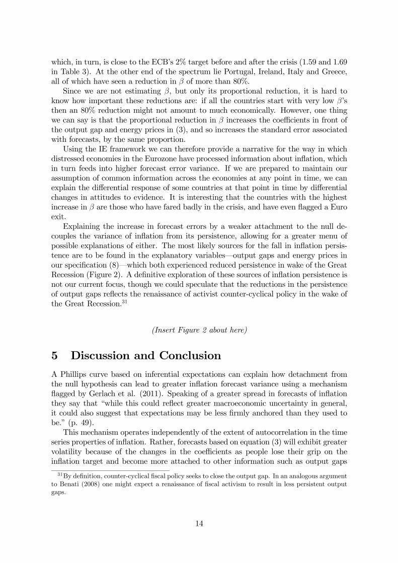
possible explanations of either. The most likely sources for the fall in inflation persis-

tence are to be found in the explanatory variables–output gaps and energy prices in

our specification (8)–which both experienced reduced persistence in wake of the Great

Recession (Figure 2). A definitive exploration of these sources of inflation persistence is

not our current focus, though we could speculate that the reductions in the persistence

of output gaps reflects the renaissance of activist counter-cyclical policy in the wake of

the Great Recession.31

(Insert Figure 2 about here)

5 Discussion and Conclusion

A Phillips curve based on inferential expectations can explain how detachment from

the null hypothesis can lead to greater inflation forecast variance using a mechanism

flagged by Gerlach et al. (2011). Speaking of a greater spread in forecasts of inflation

they say that “while this could reflect greater macroeconomic uncertainty in general,

it could also suggest that expectations may be less firmly anchored than they used to

be.” (p. 49).

This mechanism operates independently of the extent of autocorrelation in the time

series properties of inflation. Rather, forecasts based on equation (3) will exhibit greater

volatility because of the changes in the coefficients as people lose their grip on the

inflation target and become more attached to other information such as output gaps

31By definition, counter-cyclical fiscal policy seeks to close the output gap. In an analogous argument

to Benati (2008) one might expect a renaissance of fiscal activism to result in less persistent output

gaps.

14

and energy prices. As a result, we have a decoupling between experts’ forecasts of

inflation and a fall in persistence in European inflation rates.

A core part of the analysis has been to distinguish between official target credibility,

which is whether agents treat the official target as the null hypothesis, and anchoring

credibility, which is whether agents tend to anchor their belief to the null hypothesis,

whatever that might be.

As we conclude, it is therefore worth considering whether that distinction is worth-

while in practice. That is, if the two dimensions of credibility are highly correlated,

then either one could be a sufficient statistic for the other. If, for example, countries

lost anchoring credibility the moment targeted inflation left the official target, we would

be back in the world of uni-dimensional credibility, which could be described by either

the proximity to the target, or the proportion of agents anchored to it.

Our econometric results give solid evidence that this is not the case in Europe. In

Panel A of Figure 3, which is based on Table 3, we measure the percentage point loss in

official target credibility on the horizontal axis.32 This is measured by |2 − 2|−|1 − 2|,the proximity of the inflation target to the 2% official target after the crisis minus the

proximity of the inflation target before it. If this is a positive number, it means the real

inflation target is drifting further away from the official one. On the vertical axis, we

plot the proportional reduction in , which is estimated by 5 in our models. A strong

relationship (of either sign) would indicate that the distinction we have made in the

paper is of little practical importance.

In Panel B we calculated the percentage point loss in official target credibility but

do not use the 2% flagged by the ECB. Instead, we adopt the midpoint of Germany’s

‘before’ and ‘after’ inflation target, namely 1.65%, giving the percentage point loss

|2 − 165| − |1 − 165|. The reasoning here is that Germany is an important coun-try in the Eurozone and that the ECB wants inflation ‘below, but close to, 2 %’

(http://www.ecb.int/mopo/html/index.en.html), so it is natural to pick the inflation

target of a pivotal country which is, in fact, below, but close to, 2%.

(Insert Figure 3 here)

In neither panel is a strong correlation evident (for targets of 2 and 1.65 Pearson’s

is −030 and −033). To the extent that there is a weak negative association it is drivenby Ireland and Portugal–both of whom experienced a very severe loss of anchoring

credibility, in spite of the fact that their target inflation moved closer to the ECB

target (measured either as 2% or 1.65%). Overall, the two measures are more or less

independent, justifying a two-dimensional analysis of credibility.

The inferential expectations framework can therefore be used as a means of building

a two-dimensional construct for credibility, and empirically as a means of interpreting

a rise in estimated coefficients (in (3)) during the recent recession in the light of this

framework.

Our IE analysis has shown that, as a result of the Great Recession, there is no

evidence for an erosion of official target credibility in the Euro area: the ECB’s official

32We use percentage points such that a fall of the inflation target from, say, 2% to 1% would be a

50% reduction but a 1% point reduction.

15

target of 2% is still, in its own way, credible in the sense that experts believe the

monetary authorities are aiming for something close to this.

However, we have found evidence of an erosion of anchoring credibility, especially

in Portugal, Ireland, Italy and Greece, as experts are more likely to consider new

information on its merits and anchor their inflation forecasts less on the target of 2%.

References

[1] Ahrens, Ralf and Stefan Reitz (2000). “Chartist Prediction in the Foreign Exchange

Rate: Evidence from the Daily Dollar/DM Exchange Rate.” 8th World Congress

of Econometrics, Seattle, Paper No. 1683.

[2] Albinowski, Maciej, Piotr Cizkowicz, and Andrzej Rzonca (2013). “Distrust in the

ECB — product of failed crisis prevention or of inappropriate cure?” MPRA Paper

No. 48242, July.

[3] Alchian, Armen A. (1950). “Uncertainty, Evolution and Economic Theory.” Jour-

nal of Political Economy, 58(3), 211-221.

[4] Andrade, Philippe and Herve Le Bihan (2010). “Inattentive Professional Forecast-

ers.” Banque de France Working Paper No. 307, December.

[5] Barro, Robert J. and David B. Gordon (1983a). “Rules, discretion and reputation

in a model of monetary policy.” Journal of Monetary Economics, 12, 101—121.

[6] Barro, Robert J. and David B. Gordon (1983b). “A positive theory of monetary

policy in a natural rate model.” Journal of Political Economy, 91, 589—610.

[7] Blanchard, Olivier J. and Danny Quah (1989). “The Dynamic Effects of Aggregate

Demand and Supply Disturbances.” American Economic Review, 79(4), 655-673.

[8] Benati, Luca (2008). “Investigating inflation persistence across monetary regimes.”

Quarterly Journal of Economics, 123(3), 1005-1060.

[9] Borgy, Vladimir, Thomas Laubach, Jean-Stéphane Mésonnier, and Jean-Paul

Renne (2011). “Fiscal Sustainability, Default Risk and Euro Area Sovereign Bond

Yields.” Banque de France Working Paper No. 350, October, revised July 2012.

[10] Calvo, Guillermo A. (1983). “Staggered Prices in a Utility Maximizing Frame-

work.” Journal of Monetary Economics, 12, 383-398.

[11] Carroll, Christopher D. (2003). “Macroeconomic Expectations of Households and

Professional Forecasters.” Quarterly Journal of Economics, 118, 269-298.

[12] Cogley, Timothy, Giorgio E. Primiceri, and Thomas Sargent (2010). “Inflation-gap

Persistence in the US.”American Economic Journal: Macroeconomics, 2(1), 43-69.

[13] Darvas, Zsolt and Balázs Varga (2013). “Inflation Persistence in Central and East-

ern European Countries.” Corvinus University Working Paper No. 2013/2, Febru-

ary.

16

[14] Demertzis, Maria, Massimiliano Marcellino, and Nicola Viegi (2008). “A Measure

for Credibility: Tracking US Monetary Developments.” European University Insti-

tute Working Paper No. ECO 2008/38, September.

[15] Dotsey, Michael, Robert G. King, and Alexander L. Wolman (1999). “State-

dependent pricing and the general equilibrium dynamics of money and output.”

Quarterly Journal of Economics, 114, 655-690.

[16] Easaw, Joshy and Roberto Golinelli (2010). “Households Forming Inflation Expec-

tations: Active and Passive Absorption Rates.” B.E. Journal of Macroeconomics

(Contributions), 10(1).

[17] Edwards, Ward (1968). “Conservatism in human information processing.” in:

Kleinmuntz, Benjamin (ed.) Formal representation of human judgment. New York:

Wiley.

[18] Fischer, Stanley (1977). “Long-term contracts, rational expectations, and the op-

timal money supply rule.” Journal of Political Economy, 85(1), 191-205.

[19] Frankel, Jeffrey A. and Kenneth A. Froot (1986). “Understanding the US Dollar

in the Eighties: The Expectations of Chartists and Fundamentalists.” Economic

Record, Supplement, 24-38.

[20] Friedman, Milton (1968). “The Role of Monetary Policy.” American Economic

Review, 58(1), 1-17.

[21] Fuhrer, Jeffrey, C. (2011). “Inflation Persistence.” in: Friedman, Benjamin. M. and

Michael Woodford (eds.) Handbook of Monetary Economics, Volume 3A. Amster-

dam: North-Holland, 423-486.

[22] Galati, Gabriele, Steven Poelhekke, and Chen Zhou (2011). “Did the Crisis Affect

Inflation Expectations?” International Journal of Central Banking, 7(1), 167-207.

[23] Gamber, Edward N., Jeffrey P. Liebner, and Julie K. Smith (2013). “Inflation

Persistence: Revisited.” George Washington University RPF Working Paper No.

2013-002, April.

[24] Gerlach, Petra, Peter Hördahl, and Richhild Moessner (2011). “Inflation Expecta-

tions and the Great Recession.” BIS Quarterly Review, 1, 39-51.

[25] Gigerenzer, Gerd., Peter M. Todd, and The ABC Research Group (1999). Simple

Heuristics That Make Us Smart. Oxford: Oxford University Press.

[26] Gordon, Robert J. (1982). “Price inertia and policy ineffectiveness in the United

States 1890-1980.” Journal of Political Economy, 90(6), 1087-1117.

[27] Gruen, David, Adrian Pagan, and Christopher Thompson (1999). “The Phillips

Curve in Australia.” Reserve Bank of Australia Research Discussion Paper No.

1999-01, January.

17

[28] Henckel, Timo, Gordon D. Menzies, Nick Prokhovnik, and Daniel J. Zizzo (2011).

“Barro-Gordon revisited: Reputational equilibria with inferential expectations.”

Economics Letters, 12(2), 144 147.

[29] Lucas, Robert R. Jnr. (1972). “Expectations and the Neutrality of Money.” Journal

of Economic Theory, 4, 103-124.

[30] Luo, Yulei, and Eric R. Young (2010), “Risk-Sensitive Consumption and Savings

under Rational Inattention.” American Economic Journal: Macroeconomics, 2,

281-325.

[31] Lyons, Bruce, Gordon D. Menzies, and Daniel J. Zizzo (2012). “Conflicting evi-

dence and decisions by agency professionals: an experimental test in the context

of merger regulation.” Theory and Decision, 73(3), 465-499.

[32] Mankiw, N. Gregory and Ricardo Reis (2002). “Sticky Information versus Sticky

Prices: A Proposal to Replace the New Keynesian Phillips Curve.” Quarterly Jour-

nal of Economics, 117(4), 1295—1328.

[33] Menzies, Gordon D. and Daniel J. Zizzo (2009). “Inferential Expectations.” The

B.E. Journal of Macroeconomics (Advances), 9(1).

[34] OECD (2012), OECD.StatExtracts, http://stats.oecd.org/Index.aspx?QueryId=22377.

[35] O’Reilly, Gerard and Karl Whelan (2005). “Has Euro-area inflation persistence

changed over time?” Review of Economics and Statistics, 87(4), 709-720.

[36] Reis, Ricardo (2006) “Inattentive Consumers.” Journal of Monetary Economics,

53, 1761-1800.

[37] Rotemberg, Julio J. (1982). “Sticky prices in the United States.” Journal of Polit-

ical Economy, 90(6), 1187-1211.

[38] Siklos, Pierre L. (2013a). “Forecast disagreement and the anchoring of inflation

expectations in the Asia-Pacific Region.” Bank for International Settlements Paper

No. 70e, February.

[39] Siklos, Pierre L. (2013b). “Sources of Disagreement in Inflation Forecasts: An

International Empirical Investigation.” Journal of International Economics, forth-

coming.

[40] Sims, Christopher A. (2003). “Implications of Rational Inattention.” Journal of

Monetary Economics, 50, 665-690.

[41] Taylor, John (1980). “Aggregate dynamics and staggered contracts.” Journal of

Political Economy, 88(1), 1-23.

[42] Williams, John (2006). “The Phillips Curve in an Era of Well-Anchored Inflation

Expectations”, mimeo, Federal Reserve Bank of San Francisco.

[43] Yun, Tack (1996). “Nominal price rigidity, money supply endogeneity, and business

cycles.” Journal of Monetary Economics, 37(2-3), 345-370.

18

6 Appendixes

6.1 Appendix A

This appendix outlines a more general framework, and shows that lower persistence

and a greater variance contradict each other in that framework too. Let

= ∗ +

and

∗ = ∗−1 +

Using the lag operator these two equations may be rewritten as

(1− ) = + (1− )

We then have the variance,

(0) = 2 +2

1− 2and (1) = [−1] =

21− 2

So, (1)

(0)=

(1− 2) 22 + 1

If the variance of underlying inflation (say 2) increases, the variance of observed

inflation (0) becomes higher, but the autocorrelation (1) (0) increases, as in

the simple model of the main text. Nor is the problem removed if [∗ | ] =2∗ (

2∗ + 2) is somewhere in the model, since it inherits the properties of .

So, if 2 rises, so does 2∗, and with it the volatility of [

∗ | ]. However, the auto-

correlation still increases, driven by the above properties of .

6.2 Appendix B

The following appendix provides an example of how to derive the Lucas supply equation

(6) used in the main text.

Nature draws a real marginal cost shock ∼ (0 2) and price setting agent

observes a noisy signal: = + where ∼ (0 2). Considering an agent’s

belief about given , we follow Lucas (1972) to obtain agent ’s optimal guess of :

[ | ] = 22 + 2

[] +2

2 + 2 =

22 + 2

(A1)

A single producer in a centralized economy–the ‘aggregator’–demands a contin-

uum of substitutable intermediate goods indexed by over [0 1] and combines them

using CES production to produce a final good:

=

∙Z 1

0

−1

¸ −1

1 (A2)

19

Firm j maximizes profits, − R 10, subject to (A2), which yields the demand

for inputs as a function of relative prices,

= ¡¢−

(A3)

where ≡ is firm ’s relative price.

The aggregate price level is obtained by eliminating in (A2) and (A3):

1− =Z 1

0

1− (A4)

Intermediate firms all face the same production function with time-varying real

marginal costs–equal across all firms–given by = (1+) where refers

to steady state real marginal cost.

The economic interpretation of is that it is a demand shock arising from, say,

fiscal or monetary policy. Thus, captures any movement along a Phillips curve. The

zero mean of makes it consistent with the classic identification scheme where demand

shocks have zero long run effects (for example, Blanchard and Quah, 1989) and the

i.i.d. assumption is for simplicity.33

Price setters each receive a noisy signal of , denoted d:

d = (1 + + ) = (1 + ) (A5)

Firms choose to maximize real current profits, Π

¡ −

¢. Using (A3) and

assuming that firms treat aggregate output (A2) and the aggregate price level (A4)

as exogenous and non-stochastic, one obtains the solution for firm ’s optimal relative

price:

=

− 1

or,

=

− 1 (A6)

Agents set prices (A6) after forming beliefs about . We assume they use the

Lucas signal extraction solution (2) to infer from . When it comes to calculating ,

we do not require that the agents solve the whole system to arrive at a model-consistent

, since this would sit awkwardly with the assumption that they treat as exogenous

in their maximization. Instead, we assume that firms use the price level implied by

expected inflation, , similar to Yun (1996). In the main text we assume that firms

employ the publicly available consensus inflation forecast as an estimate of inflation but

some other expectation scheme, such as adaptive expectations or rational expectations,

is also possible. Introducing time subscripts, the relationship between the current price

level and expected inflation is trivially given by = −1 (1 + ).

To derive the Phillips curve, use a Lebesgue integral to rewrite (A4) as an expec-

tation over the noise conditioning on , which we will just denote [·]. That33Nothing depends on this; it just makes the signal extraction solution (A1) simple. In the main

text we allow it to exhibit autocorrelation.

20

is,

1− =

Z 1

0

1−

=

£1−

¤

"µ

− 1−1 (1 + )

¶1−#

If and are small, (1 + )1+

approximates to (1 + (1 + ) ) and we have,

1− =

"µ

− 1µ1 +

22 + 2

¶−1 (1 + )

¶1−#

=

µ

− 1 (1 + ) −1

¶1−

"µ1 +

22 + 2

¶1−#

=

µ

− 1 (1 + ) −1

¶1− µ1 +

∙2

2 + 2

¸¶1−=

µ

− 1 (1 + ) −1

¶1− µ1 +

22 + 2

[]

¶1−=

µ

− 1 (1 + ) −1

¶1− µ1 +

22 + 2

¶1−(A8)

In the first line of (A8) we use the fact that firms use the Lucas signal extraction

solution (2) for . In line 3, the small and approximation allows us to take a

linearized expectation over and then reintroduce the exponential. In lines 4 and 5

we take expectations conditional on , because we want the economy-wide effect on

inflation after the realization of . In a steady state, = 0, = −1 (1 + ), and

= . Substituting these terms into (A8) gives the steady-state solution to

(A8):

− 1 = 1 (A9)

Substituting back into (A8) and noting is second-order small we have:

1− = ((1 + ) −1)1−µ1 +

22 + 2

¶1−

Rearranging yields

−1≈ 1 + +

22 + 2

1 + = 1 + +2

2 + 2

= +2

2 + 2 (A10)

21

Defining Φ = 2 (2 + 2) yields the Lucas supply function (2) in the main text.

This supply function has the usual properties–there exists a positive relationship be-

tween inflation and an output measure and the curve shifts up or down with changes

in expected inflation.

6.3 Appendix C

This appendix creates a broader family of uniformly more conservative distributions

than the straight line with a higher gradient in the main body.

Proposition 1 If and are both continuous pdf’s of the test size over support

[0 1] and the gap − is decreasing as increases, is uniformly more conservative.

Proof. Since and are densities their difference must integrate to zero:Z 1

0

( − ) =

Z 1

0

−Z 1

0

= 0

Figure 4 plots two functions for which the difference is decreasing and integrates to

zero. It is obvious that the difference must start with a positive value and end with a

negative value. Since the difference is monotonically decreasing, the curves cross only

once.

Equation (6) in the text follows immediately for -values no greater than ∗. Forany no greater than ∗, say at 1, a shift to the more belief conservative (dashed)distribution involves integrating over a more positive function.

For a -value like 2, which lies above ∗, we note that the sum of the areas between

the curves and over [0 1] is zero, and that it would be necessary to integrate from

the intersection ∗ to unity to fully offset the positive gap − from 0 to ∗. So fora range of integration less than that–such as 0 to 2–the integral over the dashed

function must be higher.

(Insert Figure 4 about here)

Our assumption about the decreasing gap ( − ) 0 implies

for all and if we let 0 refer to changing the function such that the slope

( 0 = ) is everywhere more positive (going from the dashed to more solid line in

Figure 4), then

0 0 ∀ ∈ (0 1)

Geometrically, uniformly more conservative distributions have a greater probability

mass around zero, and the above mathematics just rules out perverse cases where the

probability mass shifts towards zero over some of the support [0 1] but away from it at

other parts of the support. The point of this analysis is that if we empirically observe

an increase in we can interpret it informally as a shifting of the probability mass

towards zero, and formally from a solid to dashed Figure-4-style distribution.

22

Table 1: Two Dimensions of Credibility

Official Target Credibility

0 at official target 0 not at official target

Anchoring High credible ?

Credibility Low ? not credible

23

Table 2: Original Non-Linear Least Squares Estimation

(estimation period: Mar-2001 to Dec-2012; quarterly data)

= 1 (1−) + 2 +3

1− 5 +

4

1− 5 +

2A: Whole Euro Area and Large 0 Reduction

Euro Area Ireland Portugal Italy Greece

1 225∗∗ 399∗∗ 305∗∗ 235∗∗ 335∗∗

(008) (028) (016) (008) (011)

2 207∗∗ 076 170∗∗ 223∗∗ 278∗∗

(013) (054) (024) (016) (014)

|2−2|− |1−2| −018 −075 −075 −013 −0573 005∗∗ −007 000 001 002

(001) (004) (004) (001) (001)

3 (1− 5) 012 035 017 011 010

4 004 −002 000 000 001

(002) (002) (002) (001) (001)

4 (1− 5) 009 012 −007 008 008

5 061∗∗ 120∗∗ 098∗∗ 094∗∗ 082∗∗

(012) (012) (023) (013) (011)

2 073 075 059 066 073

2B: Moderate 0 Reduction

Luxembourg Austria France Spain Belgium Germany Finland Netherlands

1 241∗∗ 198∗∗ 190∗∗ 334∗∗ 227∗∗ 160∗∗ 125∗∗ 218∗∗

(008) (011) (010) (013) (012) (006) (026) (017)

2 240∗∗ 239∗∗ 154∗∗ 180∗∗ 222∗∗ 169∗∗ 280∗∗ 217∗∗

(014) (018) (016) (018) (016) (008) (038) (025)

|2−2|− |1−2| −001 036 036 −114 −006 −009 005 −0023 004∗∗ 005∗∗ 004∗∗ 007∗∗ 009∗∗ 006∗∗ 003 000

(001) (002) (001) (002) (001) (001) (002) (004)

3 (1− 5) 010 010 009 013 013 006 006 011

4 000 008 001 001 −002 020∗∗ 012∗∗ 000

(001) (004) (004) (002) (006) (003) (006) (001)

4 (1− 5) 001 017 001 002 −003 021 025 003

5 062∗∗ 052∗∗ 047∗∗ 043∗∗ 030∗∗ 006 050 100∗∗

(009) (016) (017) (016) (012) (017) (025) (037)

2 078 056 063 074 081 076 032 013

Notes: Significant at 5% and 1% denoted by * and **. Standard errors in parantheses.

24

Table 3: Reduced Models

(estimation period: Mar-2001 to Dec-2012; quarterly data)

= 1 (1−) + 2 +3

1− 5 +

4

1− 5 +

3A: Whole Euro Area and Large 0 Reduction

Euro Area Ireland Portugal Italy Greece 1 225∗∗ 384∗∗ 305∗∗ 235∗∗ 335∗∗

(028) (028) (016) (017) (019) 24

2 207∗∗ 084 180∗∗ 223∗∗ 278∗∗

(030) (056) (020) (021) (023) 18

|2−2|− |1−2| −018 −068 −085 −013 −0573 005∗∗ 000 000 001 001

(002) (004) (004) (001) (001) 09

3 (1− 5) 012 035 017 011 010

4 004 000 000 001

(007) (002) (002) (001) 19

4 (1− 5) 009 014 008 008

5 061∗∗ 09999∗∗ 09999∗∗ 094∗∗ 082∗∗

(020) (014) (015) 12

2 073 075 059 066 073

3B: Moderate 0 Reduction

Luxembourg Austria France Spain Belgium Germany Finland Netherlands

1 242∗∗ 198∗∗ 191∗∗ 337∗∗ 225∗∗ 159∗∗ 125∗∗ 218∗∗

(016) (028) (019) (025) (027) (011) (067) (044)

2 236∗∗ 239∗∗ 152∗∗ 175∗∗ 226∗∗ 169∗∗ 280∗∗ 217∗∗

(017) (031) (020) (029) (029) (013) (056) (041)

|2−2|− |1−2| −001 036 036 −112 001 −010 005 −0023 004∗∗ 005∗∗ 005∗∗ 008∗∗ 009∗∗ 006∗∗ 003 000

(001) (002) (001) (002) (001) (001) (002) (002)

3 (1− 5) 010 010 009 013 012 006 006 011

4 008 020∗∗ 012∗∗ 000

(007) (004) (009) (003)

4 (1− 5) 017 020 025 003

5 062∗∗ 052∗∗ 046∗∗ 039∗∗ 030∗∗ 050 100∗∗

(009) (020) (015) (016) (011) (041) (024)

2 078 056 063 077 082 076 032 013

Notes: Significant at 5% and 1% denoted by * and **. Standard errors (in parantheses) are OLS for Ireland

and Portugal and feasible GLS otherwise.

25

Figure 1: Euro Area Inflation AR(1) Coefficients

Notes: Year average inflation, 7-year rolling regression window, no constant. Datastream.

Figure 2: Euro Area AR(1) Coefficients

Notes: Year average variables, 7-year rolling regression window, no constant. Datastream.

26

Figure 3: Independence of Anchoring Credibility and Official Target

Credibility

Notes: Regression output. % pt. loss OFFICIAL TARGET CRED is |2 − 2|− |1 − 2|in the left panel and |2 − 165|− |1 − 165| in the right panel, and positive values indicatea drift away from the ECB target. Prop loss ANCHOR CRED is the decline in estimated

by 5 in our econometric models.

Figure 4: Two Examples of Probability Density Functions for

27