the initial stage of transition in pipe flow: role of ... · the initial stage of transition in a...
TRANSCRIPT
J. Fluid Mech. (2004), vol. 517, pp. 131–165. c© 2004 Cambridge University Press
DOI: 10.1017/S0022112004000825 Printed in the United Kingdom
131
The initial stage of transition in pipe flow:role of optimal base-flow distortions
By M. I. GAVARINI,1 A. BOTTARO 2†AND F. T. M. NIEUWSTADT1‡
1J. M. Burgers Centre, Lab. Aero & Hydrodynamics, Delft University of Technology,2628 CA Delft, The Netherlands
2Institute de Mecanique des Fluides de Toulouse, Allee du Pr. Camille Soula, 31400 Toulouse, France
(Received 27 October 2003 and in revised form 24 June 2004)
We explore the spatial growth of disturbances developing on top of a base flow givenby the Hagen–Poiseuille profile, which has been modified by a small axisymmetricand axially invariant distortion. Such deviations from the ideal parabolic profilemay, for instance, occur in experiments as a result of experimental uncertainties.The optimal distortion (i.e. the distortion with a prescribed norm that induces themaximum growth rate) is computed by a variational technique. Unstable modes arefound to exist for very small values of the norm of the deviation at low Reynoldsnumbers, and the instability is governed by an inviscid mechanism. The growth ofthese modes and the ensuing transition to turbulence is then studied by means ofdirect numerical simulations. Two possible paths of transition are found, one basedon the exponential amplification of axisymmetric disturbances and the subsequentformation of �-vortices and the other based on the growth and breakdown ofstreamwise streaks.
1. IntroductionIn the transition process from laminar to turbulent flow in a cylindrical pipe, at
least two stages can be distinguished: the initial and the late stage. The initial stageis related to the receptivity, i.e. the way the flow filters incoming disturbances, andto their initial linear growth into finite-amplitude perturbations, for which eventuallynonlinear mechanisms (late stage) become important. Recently, much progress hasbeen made in our understanding of the late stage of transition. Both experiments(Han, Tumin & Wygnanski 2000) and numerical simulations (Reuter & Rempfer2000) have shown that in pipe flow this late stage is accompanied by the formationof �-like vortices characterized by strong shear layers and by spikes in the temporaltraces of the velocity. These spikes are associated to ring-like vortices that separatefrom the tips of the large �-vortices. Similar structures have also been found in thelate stages of transition in boundary layers, either in the K-, N- or O-regimes ofbreakdown (see Berlin, Wiegel & Henningson 1999). These observations indicate thata considerable degree of similarity exists in the late stage of transition in a pipe andin a boundary layer.
† Present address: DIAM, Universita di Genova, via Montallegro 1, 16145 Genova, Italy.‡ Author to whom correspondence should be addressed: e-mail [email protected]
132 M. I. Gavarini, A. Bottaro and F. T. M. Nieuwstadt
The initial stage of transition in a flat-plate boundary layer in the presence of acou-stic disturbances in the free stream and of roughness elements on the surface usuallystarts with the excitation of unstable Tollmien–Schlichting (TS) waves if the Reynoldsnumber exceeds a critical value. When these two-dimensional TS waves reach a suffi-ciently large amplitude, a three-dimensional secondary instability develops. This in-stability produces a streamwise component of the vorticity which eventually leads tothe formation of �-vortices, i.e. to the start of the late stage described above. However,when the disturbance environment is dominated by reasonably high levels of free-stream turbulence, Matsubara & Alfredsson (2001) have shown that transition closelyapproaches the oblique transition path (see Berlin, Lundbladh & Henningson 1994),in which the initial exponential growth is by-passed by another linear and strongeramplification mechanism, i.e. the non-modal growth of streamwise-elongated struc-tures. This is an example of the ‘weak-disturbance by-pass’ introduced by Morkovin(1993). In the presence of even higher levels of free-stream turbulence, the whole initialstage of linear growth is by-passed and the late stage of transition sets in immediately.This has been categorized as the ‘strong-disturbance by-pass’ by Morkovin.
For the cylindrical pipe geometry, much less is known about the initial stage oftransition, one of the reasons being that there are no linearly unstable modes of theTS kind. Analytical treatment of pipe flow transition, through the classical normal-mode approach, has shown that the fully developed parabolic Hagen–Poiseuilleprofile is linearly stable at all Reynolds numbers, Re (see Lessen, Sadler & Liu1968; Davey & Drazin 1969; Garg & Rouleau 1972). Although a rigorous proof ofstability exists only for axisymmetric disturbances (Herron 1991), there is very strongevidence (e.g. Salwen, Cotton & Grosch 1980; Meseguer & Trefethen 2003) that alllinear perturbations decay exponentially for all values of Re and for any value ofthe streamwise and azimuthal wavenumbers α and m. Nevertheless, in experiments,transition to turbulence in pipe flow is typically observed for Re � Recrl
. Here, Recrlis
the lower limit of the critical (we should rather say ‘transitional’) Reynolds number,which means that below Recrl
all finite perturbations decay. The value of Recrlhas
been estimated experimentally to lie in the range 1760<Recrl< 2300. We speak in
this case of subcritical transition to turbulence, as transition occurs at values of theReynolds numbers, for which linear theory indicates stability.
On the other hand, in very carefully performed experiments, conceived to exclude allcauses for external perturbations, laminar Hagen–Poiseuille flow can be maintainedup to very large values of the Reynolds number. In the very first experimentsconducted by Reynolds in 1880, for instance, a transitional value of the parameter,that eventually became known as the Reynolds number, close to 13000 was observed.Reynolds’ original observations were published three years later (Reynolds 1883)and for a long time his results remained unchallenged and unexplained by theory.In more recent times, Pfenniger (1961) reports Recru
� 105, where Recrudenotes the
upper limit of the critical Reynolds number. Different values of Recruare reported for
individual experiments (see, for example, Draad, Kuiken & Nieuwstadt 1998). For allthese experiments, however, it turns out that Recru
>Redev, where Redev is the value ofthe Reynolds number, for which the velocity profile at the end of the pipe deviatesby less than 1% from the theoretical Hagen–Poiseuille profile. This could imply thatthe transition process found in these experiments may not be considered as naturaltransition of cylindrical pipe flow, but rather as the result of the instabilities of thedeveloping boundary layer on the wall of the pipe. On the other hand, these highvalues of Recru
do not contradict the estimate Recr → ∞ of linear stability theory forthe fully developed flow.
Initial stage of transition in pipe flow 133
Another route to transition in pipe flow has been reported in the experiments ofDarbyshire & Mullin (1995); Eliahou, Tumin & Wygnanski (1998); Draad et al. (1998)and the numerical simulations of Ma et al. (1999) and Reuter & Rempfer (2000). Inthis case, transition is forced by the introduction of finite disturbances at the wall, inparticular by periodic blowing and suction through slots in the pipe wall. Althoughthe perturbations are finite, they are nevertheless small and, without additionalamplification, they should decay as predicted by the classical linear eigen-analysis.However, it has been suggested by various authors (Boberg & Brosa 1988; Bergstrom1992, 1993; Trefethen et al. 1993; Schmid & Henningson 1994) that, in this case, thenon-normality of the linearized Navier–Stokes operator can play an important role,since it implies potential for strong initial amplification of disturbances, also denotedas transient growth. As a result of this growth, the disturbance amplitude may reacha level for which nonlinear interactions are triggered and the eventual viscous decaypredicted by the linear asymptotic analysis is overcome. The scenario of amplificationof small finite perturbations through transient growth in pipe flow was, for instance,suggested by Ma et al. (1999) and O’Sullivan & Breuer (1994a , b) based on numericalsimulations. Adopting the definitions that were introduced above for a boundary-layer flow, this transition scenario could be referred to as by-pass transition, since thelinear amplification of disturbances requires a by-pass of the single mode growth. Theestimates for Recrl
that have been obtained following this by-pass scenario lie in therange of 1760< Recrl
< 2300, which has already been mentioned and this provides anencouraging argument for the transient-growth picture. It should also be noted thatthese values still differ strongly from the lower bound for transition, i.e. Recre
= 81.49,obtained through the energy method (Joseph & Carmi 1969; Schmid & Henningson1994).
The non-normality of the linearized operator has another important consequence,i.e. the high sensitivity of some of its eigenvalues to perturbations, such as, forexample, distortions in the base flow (Bottaro, Corbett & Luchini 2003). Such a strongsensitivity is clearly observed in the experiments by Darbyshire & Mullin (1995), whoshow a broad intermittent range of turbulent flow and decaying perturbations inthe disturbance amplitude versus Reynolds-number space. In the carefully controlledexperiments by Eliahou et al. (1998), it was noted that, by exciting the azimuthalperiodic modes m = ±2 with time-periodic suction and blowing through slots inthe pipe wall, transition could be triggered at Re =2200 only for sufficiently large-disturbance amplitudes. Eliahou et al. (1998) concluded with the suggestion that‘transition to turbulence in a fully developed pipe Poiseuille flow can occur only afterthe parabolic velocity profile became distorted.’
Base-flow deviations from the theoretical parabolic Hagen–Poiseuille profile canbe ascribed to a variety of physical reasons. They are likely to occur in anyexperimental set-up owing to surface-roughness effects, external volume forces, inflowinhomogeneities, and so on. Even when the theoretical profile is linearly stable, as isthe case for the Hagen–Poiseuille flow, it is possible that small base-flow distortionsrender the flow linearly unstable. This possible scenario of instability has alreadybeen examined by Gill (1965) in an effort to explain some laboratory measurements.
The objective of the present work is to show by means of theory and numericalsimulations that the sensitivity of the eigenmodes to small distortions in the baseflow can be a cause for initial exponential growth of perturbations. It is expectedthat those eigenvalues, which show the highest sensitivity to infinitesimal variationsin the base flow, are the most affected and can become unstable. These so-calledmost ‘receptive’ eigenvalues have been recently identified by Tumin (1996) through a
134 M. I. Gavarini, A. Bottaro and F. T. M. Nieuwstadt
spatial analysis which employs the direct and adjoint stability operator. Our analysishere differs from that of Tumin because, given these most ‘receptive’ eigenvalues,we identify so-called ‘optimal’ base-flow deviations, i.e. those distortions from theHagen–Poiseuille profile, which maximize the instability of the flow in a way tobe described shortly. It will be shown that deviations with a very small (butfinite) norm are already sufficient for the modified flow to become exponentiallyunstable at low Reynolds numbers. This exponential instability, which can also act incombination with transient-growth mechanisms, may amplify disturbances to a levelwhere eventually nonlinear interactions can take over bringing the flow to the latestage of transition.
In the next two sections, we describe the theory of the optimally perturbed baseflow. First, a method based on spatial eigen-analysis is presented to determine thesensitivity of individual eigenvalues to variations introduced in the base flow. Then astandard variational technique is used to determine the optimal base-flow deviations,i.e. those deviations that can best destabilize the flow. Finally, in § 4, we describeresults from direct simulations of the nonlinear governing equations carried out tostudy the evolution of unstable eigenmodes, and discuss the viability of the transitionscenario identified.
2. The theoryAs the starting point of our analysis we introduce a cylindrical coordinate system
(x, r, θ). Here, x, r and θ denote the axial, radial and azimuthal directions, respectively,and u, v and w the corresponding velocity components. The laminar solution to theincompressible Navier–Stokes equations for a cylindrical pipe geometry is the well-known Hagen–Poiseuille flow, which in non-dimensional form, using the centrelinevelocity Umax and the pipe radius R as scales, reads:
V (r) = U (r)ex = (1 − r2)ex, P (x) = P0 − 4
Rex, (2.1)
where P0 is the static pressure at x =0 and ex is the unit vector in the x-direction. TheReynolds number is Re = Umax R/ν. Linearization of the full Navier–Stokes equationaround the laminar solution U produces:
∂u
∂x+
1
r
∂ (rv)
∂r+
1
r
∂w
∂θ= 0, (2.2a)
∂u
∂t+ U
∂u
∂x+ v
dU
dr= −∂p
∂x+
1
Re∇2u, (2.2b)
∂v
∂t+ U
∂v
∂x= −∂p
∂r+
1
Re
(∇2v − v
r2− 2
r2
∂w
∂θ
), (2.2c)
∂w
∂t+ U
∂w
∂x= −1
r
∂p
∂θ+
1
Re
(∇2w − w
r2+
2
r2
∂v
∂θ
), (2.2d )
with
∇2 =∂2
∂x2+
1
r
∂
∂r
(r
∂
∂r
)+
1
r2
∂2
∂θ2. (2.3)
Next, we assume the disturbance quantities v = (u, v, w) and p to be of the form:
v (r, θ, x, t) = v (r, x; m, ω) ei(mθ−ωt),
p (r, θ, x, t) = p (r, x; m, ω) ei(mθ−ωt),
Initial stage of transition in pipe flow 135
where m is the azimuthal wavenumber, ω the dimensionless circular frequency andv =(u, v, w) and p the complex disturbance amplitudes. Following Tumin (1996),two auxiliary variables are introduced, namely vx = ∂v/∂x and wx = ∂w/∂x. Theequations (2.2a)–(2.2d ) can then be rewritten as a system of first-order differentialequations in x, for which the vector of the unknowns is given by a (x, r; m, ω, Re) =(v, vx, u, p, w, wx). The resulting system in compact notation reads:
∂a∂x
= C0a + C1
∂a∂r
+ C2
∂2a∂r2
, (2.4)
where Ck (k = 0, 1, 2) are 6 × 6 coefficient matrices whose non-zero entries are givenin Appendix A.
In a spatial stability analysis, the frequency ω is a real parameter and the solutionto system (2.4) is assumed to behave as:
a(x, r; m, ω, Re) = aα(r; m, ω, Re)eiαx.
Introduction into (2.4) results in the following eigenvalue problem:
iαaα = Laα, (2.5)
where α is the complex eigenvalue, whose real and imaginary parts give, respectively,the wavenumber and the growth rate of the eigenmode in the streamwise direction.The linear operator L is given by:
L =
2∑k=0
Ck
dk
drk.
At the pipe wall, the no-slip boundary condition is assumed:
r = 1: a1 ≡ v = 0, a3 ≡ u = 0, a5 ≡ w = 0
and, as a result, the other variables must satisfy the conditions:
r = 1: a′4 ≡ p′ =
1
Rea′′
1 , a2 ≡ vx = 0, a6 ≡ wx = 0,
in which primes indicate derivation with respect to the radial coordinate.Although r =0 is not a physical boundary, it is a numerical boundary and the
condition that must be imposed at the pipe centreline is that all flow quantitiesremain bounded. This is accomplished by the following conditions for r → 0, as afunction of the azimuthal wavenumber m:
m = 0 : a1 = a′3 = a5 = 0, ⇒ a2 = a′
4 = a6 = 0,
m = ±1 : a′1 = a3 = a′
5 = 0, ⇒ a′2 = a4 = a′
6 = 0,
|m| > 1 : a1 = a3 = a5 = 0, ⇒ a2 = a4 = a6 = 0.
The numerical solution of the resulting eigenvalue problem is achieved by theuse of a Chebyshev pseudospectral collocation technique. To determine the adequatenumber (N +1) of Chebyshev polynomials, spectra obtained with N = 64 and N = 128collocation points have been compared. With N = 64, the first 60 eigenvalues, takenin order of increasing absolute value of their imaginary part, have been found to besufficiently well resolved. When it was necessary to investigate higher eigenvalues inthe spectrum, 128 collocation points have been used.
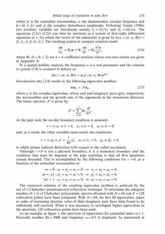
As an example, in figure 1, the spectrum of eigenvalues for azimuthal index m =1,Reynolds number Re =3000 and frequency ω =0.5 is displayed. As mentioned in
136 M. I. Gavarini, A. Bottaro and F. T. M. Nieuwstadt
0 0.5 1.0 1.5 2.0
–4
–2
0
2
4
6
8
αr
αi
21
Figure 1. Spatial spectrum of eigenvalues for Hagen–Poiseuille flow at Re = 3000, m= 1,ω =0.5. The large circle includes the two most receptive eigenvalues (cf. § 3.1.) The numbers 1and 2 denote the two main branches of eigenvalues (represented respectively by + and ×, todistinguish them from the rest of the spectrum, �).
§ 1, all available evidence indicates that linear modes are stable. The presence ofsome eigenvalues with αi < 0 does not imply instability; these modes are simplypropagating upstream, reflecting the fact that the initial-value problem for spatiallydeveloping disturbances is not well posed. The property of upstream and downstreampropagation of some of these modes has been recently verified in the numerical simula-tions by Ma et al. (1999). In figure 1, for the purpose of subsequent data presentation,we have labelled with 1 and 2 the two neighbouring branches belonging to the twomain groups of eigenvalues and we have indicated them with different symbols.
3. Optimal base-flow deviations3.1. The sensitivity function GU
Let us introduce an infinitesimal real variation δU in the base-flow velocity profile U
and compute the corresponding variation in the eigenvalues δα and eigenfunctionsδaα of system (2.5). The variational system reads:
iδα aα + iα δaα = δL aα + L δaα, (3.1)
where δL is given in matrix form by:
δL =
0 0 0 0 0 00 ReδU 0 0 0 00 0 0 0 0 0(
δU
r− δU ′
)0 0 0
imδU
r0
0 0 0 0 0 00 0 0 0 0 ReδU
+
0 · · · 00 · · · 00 · · · 0
δU · · · 00 · · · 00 · · · 0
d
dr.
Initial stage of transition in pipe flow 137
In the analysis that follows, we will make use of a scalar product between two vectorsf and g, defined as:
( f , g) ≡∫ 1
0
r g† f dr =
∫ 1
0
r (g∗1f1 + g∗
2f2 + · · · + g∗6f6)dr,
where the superscripts † and ∗ denote, respectively, the conjugate transpose and thecomplex conjugate. Upon taking the inner product of both sides of the variationalsystem (3.1) with a function bα:
(iδα aα, bα) + (iα δaα, bα) = (δL aα, bα) + (L δaα, bα) , (3.2)
and after some manipulations, including the integration by parts of the term δU ′ inδL, (3.2) can be reduced to the form:
iδα
∫ 1
0
r b†αaα dr + (δaα, −iα∗bα) = i
∫ 1
0
r GUδU dr + (δaα, Labα) ,
with GU given by:
GU = −i Re b∗2a2 + b∗
4
[ma5 − 2i a1
r− 2ia′
1
]− i a′∗
4 a1 − i Re b∗6a6. (3.3)
The function bα is now chosen to be a solution of the adjoint eigenvalue problem,defined by
−i α∗bα = Labα =
2∑k=0
(−1)k1
r
dk(rC†kbα)
drk,
with the following boundary conditions for r =1:
b2 = b4 = b6 = 0 ⇒ b′2 = b5 = 0, b1 +
1
Reb′
4 = 0
and for r → 0
m = 0 : b2 = b′4 = b6 = 0 ⇒ b1 = b5 = 0, − 3
2b′′
2 + b′3 = 0;
m = ±1 : b′2 = b4 = b′
6 = 0, ⇒ b3 = 0, b1 + im b5 = 0, b′5 +
im
2Reb′′
4 = 0;
|m|> 1 : b2 = b4 = b6 = 0 ⇒ b3 = 0, b1 +1
Reb′
4 = 0, b5 +im
Reb′
4 = 0.
The functions bα and aα are normalized so that the bi-orthonormality condition issatisfied:
(aα, bβ) =
∫ 1
0
r b†β aα dr = δαβ.
With this choice for bα , the variation δα in the eigenvalue can be evaluated from (3.2)as:
δα =
∫ 1
0
rGUδU dr, (3.4)
where GU represents the sensitivity function of each eigenvalue α to base-flowvariations.
Relation (3.4) shows that (rGU ) can be interpreted as an integrating factor betweena variation introduced in the base flow δU and the corresponding variation in theeigenvalue δα. Depending on the property of GU , it is possible that small base-flow
138 M. I. Gavarini, A. Bottaro and F. T. M. Nieuwstadt
10 20 30 40 50 60 70 800
0.5
1.0
1.5
2.0
2.5
(×104)
Mode number
rGU ∞
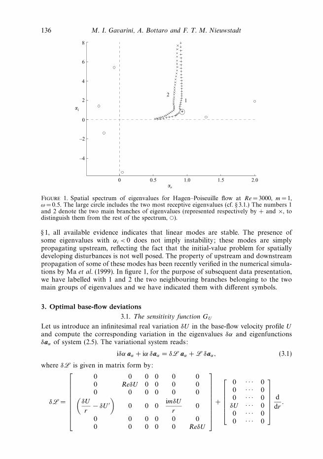
Figure 2. Infinity norm of (rGU ) for the eigenvalues shown in figure 1, numbered in orderof increasing |αi |.
deviations render the flow linearly unstable. Our interest is therefore primarily focusedon those eigenvalues, for which the sensitivity function GU is large. By solving thedirect and adjoint problem, the function GU has been computed for all eigenvaluesof the spectrum, according to the definition (3.3). The results for the infinity norm,i.e. the largest absolute value, of (rGU ) are presented in figure 2 for the first 80eigenvalues of the spectrum shown in figure 1. Here, the symbols correspond to thoseused in figure 1 to denote the eigenvalue branches.
As can be seen from figure 2, the least stable eigenvalue has a very small infinitynorm of the sensitivity function, while the maximum values for GU are attainedby the eigenmodes numbered 22, for which α =0.9279 + 0.8111i, and 24, for whichα = 0.9272 + 0.8791i (the corresponding eigenvalues are encircled in figure 1). It alsoappears that the modes corresponding to the first family of eigenvalues (indicated bya ‘+’ sign) are more sensitive than those belonging to the second family, at least up tomode 58. The higher sensitivity found for the modes belonging to the first family, andin particular for modes 22 and 24, agrees with the result reported by Tumin (1996),who indicates that precisely those modes are most receptive to periodic suction andblowing through a slot at the wall.
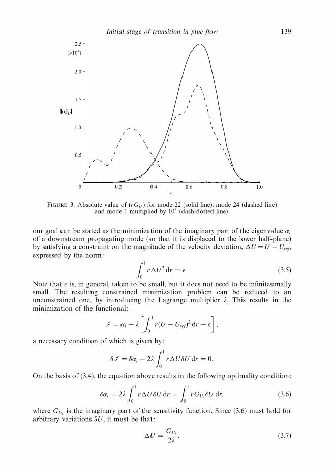
Figure 3 illustrates the absolute value of (rGU ) as a function of the radial directionfor these two most sensitive eigenmodes and also for the least stable eigenmode.The sensitivity functions for modes 22 and 24 have a maximum close to the wall(around r = 0.66) and this maximum is about three orders of magnitude larger thanthe maximum value of the least stable mode, which is located closer to the centreline.
3.2. The ‘optimally’ perturbed base flow
Our interest now shifts to finding ‘optimal’ deviations from the ideal base flow, whichin our case is the Hagen–Poiseuille flow and which will be called Uref from now on.‘Optimal’ in this case means base-flow distortions which lead to exponentially growingperturbations, but at the same time minimize the deviation from Uref. Equivalently,
Initial stage of transition in pipe flow 139
0.2 0.4 0.6 0.8 1.00
0.5
1.0
1.5
2.0
2.5
r
(×104)
rGU
Figure 3. Absolute value of (rGU ) for mode 22 (solid line), mode 24 (dashed line)and mode 1 multiplied by 103 (dash-dotted line).
our goal can be stated as the minimization of the imaginary part of the eigenvalue αi
of a downstream propagating mode (so that it is displaced to the lower half-plane)by satisfying a constraint on the magnitude of the velocity deviation, U = U − Uref,expressed by the norm: ∫ 1
0
rU 2 dr = ε. (3.5)
Note that ε is, in general, taken to be small, but it does not need to be infinitesimallysmall. The resulting constrained minimization problem can be reduced to anunconstrained one, by introducing the Lagrange multiplier λ. This results in theminimization of the functional:
I = αi − λ
[∫ 1
0
r(U − Uref)2 dr − ε
],
a necessary condition of which is given by:
δI = δαi − 2λ
∫ 1
0
rUδU dr = 0.
On the basis of (3.4), the equation above results in the following optimality condition:
δαi = 2λ
∫ 1
0
rUδU dr =
∫ 1
0
rGUiδU dr, (3.6)
where GUiis the imaginary part of the sensitivity function. Since (3.6) must hold for
arbitrary variations δU , it must be that:
U =GUi
2λ. (3.7)
140 M. I. Gavarini, A. Bottaro and F. T. M. Nieuwstadt
0.4 0.6 0.8 1.0 1.2 1.4 1.6 1.8 2.0
0
0.5
1.0
1.5
2.0
αr
a
b
c
αi
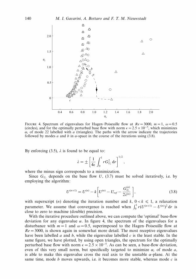
Figure 4. Spectrum of eigenvalues for Hagen–Poiseuille flow at Re = 3000, m= 1, ω = 0.5(circles), and for the optimally perturbed base flow with norm ε = 2.5 × 10⁻⁵, which minimizesαi of mode 22 labelled with a (triangles). The paths with the arrow indicate the trajectoriesfollowed by modes a and b in α-space in the course of the iterations using (3.8).
By enforcing (3.5), λ is found to be equal to:
λ = ±[
1
4ε
∫ 1
0
rG2Ui
dr
]1/2
,
where the minus sign corresponds to a minimization.Since GUi
depends on the base flow U , (3.7) must be solved iteratively, i.e. byemploying the algorithm:
U (n+1) = U (n) − k
[U (n) − Uref −
G(n)Ui
2λ(n)
], (3.8)
with superscript (n) denoting the iteration number and k, 0 <k � 1, a relaxation
parameter. We assume that convergence is reached when∫ 1
0r(U (n+1) − U (n))2 dr is
close to zero to machine (double) precision.With the iterative procedure outlined above, we can compute the ‘optimal’ base-flow
deviation for any eigenvalue α. In figure 4, the spectrum of the eigenvalues for adisturbance with m =1 and ω = 0.5, superimposed to the Hagen–Poiseuille flow atRe = 3000, is shown again in somewhat more detail. The most receptive eigenvalueshave been labelled a and b, while the eigenvalue labelled c is the least stable. In thesame figure, we have plotted, by using open triangles, the spectrum for the optimallyperturbed base flow with norm ε = 2.5 × 10⁻⁵. As can be seen, a base-flow deviation,even of this very small norm, but specifically targeted to minimize αi of mode a,is able to make this eigenvalue cross the real axis to the unstable α-plane. At thesame time, mode b moves upwards, i.e. it becomes more stable, whereas mode c is
Initial stage of transition in pipe flow 141
0 0.1 0.2 0.3 0.4 0.5 0.6 0.7 0.8 0.9 1.0–0.8
–0.6
–0.4
–0.2
0
0.2
0.4
0.6
0.8
1.0
r
(U'/r
)'/20
, U s1o
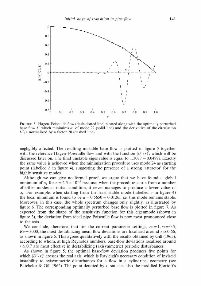
Figure 5. Hagen–Poiseuille flow (dash-dotted line) plotted along with the optimally perturbedbase flow U which minimizes αi of mode 22 (solid line) and the derivative of the circulationU ′/r normalized by a factor 20 (dashed line).
negligibly affected. The resulting unstable base flow is plotted in figure 5 togetherwith the reference Hagen–Poiseuille flow and with the function (U ′/r)′, which will bediscussed later on. The final unstable eigenvalue is equal to 1.3077 − 0.0499i. Exactlythe same value is achieved when the minimization procedure uses mode 24 as startingpoint (labelled b in figure 4), suggesting the presence of a strong ‘attractor’ for thehighly sensitive modes.
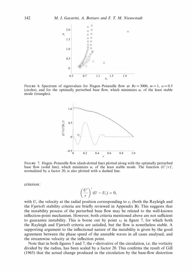
Although we can give no formal proof, we argue that we have found a globalminimum of αi for ε = 2.5 × 10⁻⁵ because, when the procedure starts from a numberof other modes as initial condition, it never manages to produce a lower value ofαi . For example, when starting from the least stable mode (labelled c in figure 4)the local minimum is found to be α = 0.5650 + 0.0126i, i.e. this mode remains stable.Moreover, in this case, the whole spectrum changes only slightly, as illustrated byfigure 6. The corresponding optimally perturbed base flow is plotted in figure 7. Asexpected from the shape of the sensitivity function for this eigenmode (shown infigure 3), the deviation from ideal pipe Poiseuille flow is now most pronounced closeto the axis.
We conclude, therefore, that for the current parameter settings, m =1, ω =0.5,Re = 3000, the most destabilizing mean flow deviations are localized around r � 0.66,as shown in figure 5. This agrees qualitatively with the results obtained by Gill (1965),according to whom, at high Reynolds numbers, base-flow deviations localized aroundr � 0.7 are most effective in destabilizing (axisymmetric) periodic disturbances.
As shown in figure 5, the optimal base-flow deviation produces five points forwhich (U ′/r)′ crosses the real axis, which is Rayleigh’s necessary condition of inviscidinstability to axisymmetric disturbances for a flow in a cylindrical geometry (seeBatchelor & Gill 1962). The point denoted by s1 satisfies also the modified Fjørtoft’s
142 M. I. Gavarini, A. Bottaro and F. T. M. Nieuwstadt
0.3 0.7 1.1 1.5 1.9
0
0.5
1.0
1.5
2.0
αr
αi
Figure 6. Spectrum of eigenvalues for Hagen–Poiseuille flow at Re = 3000, m= 1, ω = 0.5(circles), and for the optimally perturbed base flow, which minimizes αi of the least stablemode (triangles).
0 0.2 0.4 0.6 0.8 1.0–0.5
0
0.5
1.0
r
(U'/r
)'/20
, U
s2
Figure 7. Hagen–Poiseuille flow (dash-dotted line) plotted along with the optimally perturbedbase flow (solid line), which minimizes αi of the least stable mode. The function (U ′/r)′,normalized by a factor 20, is also plotted with a dashed line.
criterion: (U ′
r
)′
(U − Us) < 0,
with Us the velocity at the radial position corresponding to s1 (both the Rayleigh andthe Fjørtoft stability criteria are briefly reviewed in Appendix B). This suggests thatthe instability process of the perturbed base flow may be related to the well-knowninflection-point mechanism. However, both criteria mentioned above are not sufficientto guarantee instability. This is borne out by point s2 in figure 7, for which boththe Rayleigh and Fjørtoft criteria are satisfied, but the flow is nonetheless stable. Asupporting argument to the inflectional nature of the instability is given by the goodagreement between the phase speed of the unstable waves in all cases analysed, andthe streamwise velocity at the inflection point.
Note that in both figures 5 and 7, the r-derivative of the circulation, i.e. the vorticitydivided by the radius, has been scaled by a factor 20. This confirms the result of Gill(1965) that the actual change produced in the circulation by the base-flow distortion
Initial stage of transition in pipe flow 143
0.1 0.2 0.3 0.4 0.5 0.6 0.7 0.8 0.9 1.00
0.2
0.4
0.6
0.8
1.0
1.2
r
u,
5v
,w
, 1
0p
s1
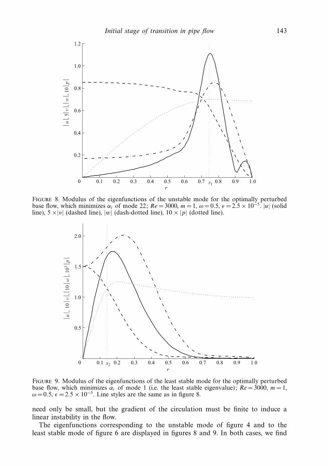
Figure 8. Modulus of the eigenfunctions of the unstable mode for the optimally perturbedbase flow, which minimizes αi of mode 22; Re =3000, m= 1, ω = 0.5, ε = 2.5 × 10⁻⁵. |u| (solidline), 5 ×|v| (dashed line), |w| (dash-dotted line), 10 × |p| (dotted line).
0.1 0.2 0.3 0.4 0.5 0.6 0.7 0.8 0.9 1.00
0.5
1.0
1.5
2.0
r
u,
10
v,
10w
, 1
03 p
s2
Figure 9. Modulus of the eigenfunctions of the least stable mode for the optimally perturbedbase flow, which minimizes αi of mode 1 (i.e. the least stable eigenvalue); Re= 3000, m= 1,ω = 0.5, ε = 2.5 × 10⁻⁵. Line styles are the same as in figure 8.
need only be small, but the gradient of the circulation must be finite to induce alinear instability in the flow.
The eigenfunctions corresponding to the unstable mode of figure 4 and to theleast stable mode of figure 6 are displayed in figures 8 and 9. In both cases, we find
144 M. I. Gavarini, A. Bottaro and F. T. M. Nieuwstadt
that a peak in axial velocity u occurs close to the points s1 and s2 where (U ′/r)′
vanishes.It could be argued that these newly obtained base flows, as shown in figures 5
and 7, are not solutions of the unforced Navier–Stokes equations. However, they aresolutions if, for example, a small volume force fx = − ∇2(U )/Re or alternativelya small pressure deviation (equal to −fxx) are applied in the axial direction. Inpractice, several mechanisms could act as external forcing, allowing for solutionsto the Navier–Stokes equations different from the Hagen–Poiseuille flow, at leastlocally. A few examples are the Coriolis force that Draad et al. (1998) had to dealwith in their experiments, convection due to (small) temperature differences betweenthe fluid in the pipe and the outside ambient, or again roughness elements or localdisturbances in the geometry, such as curvature due to small bends along the pipe ora slightly non-circular pipe cross-section (see, for instance the work of Davey (1978)and Kerswell & Davey (1996) on nearly circular elliptical pipes). We can also considernon-stationary phenomena that may occur when, for instance, the pressure gradientchanges as a function of time so that the mean flow deviates from the parabolic profilefor some time. If, as a consequence of any of these mechanisms, the modified flowcan be established and can persist over a sufficiently long axial distance, transitioncan be triggered by the exponential instability.
The results discussed above can be interpreted as a possible initial stage in thetransition process in cylindrical pipe flow. A slightly imperfect base flow allowsexponential growth of small disturbances. When these disturbances are allowed tobecome large enough, they may trigger the nonlinear interactions characteristic ofthe final stage of transition. We will return to this possible scenario for transition in§ 4 when we discuss the numerical simulations.
3.3. Dependence on Re, ω, m and ε
In the previous section, we have considered the optimal base-flow deviation only for afixed setting of parameters. Let us now consider the effect of varying these parameters.
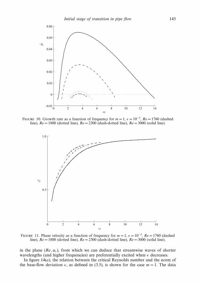
In figure 10, the growth rate, −αi , is plotted as a function of the frequency ω for aperturbation with m =1 and for different values of the Reynolds number. Each pointin the curve represents the growth rate of the most sensitive mode for a base flow,which (optimally) deviates from the Hagen–Poiseuille profile by a function U ofnorm ε =10−5. Clearly, a larger band of frequencies becomes unstable as Re increases.For the chosen values of m and ε the exponential amplification of one eigenmodestarts already at Re somewhat below 1760 with αr � 4 and ω � 3.5. In figure 11,the corresponding values of the phase velocity, cp = ω/αr , are displayed. The wavesare dispersive and their speed of propagation increases with ω. Furthermore, as ω
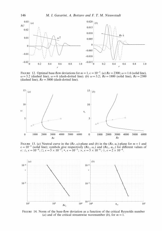
increases or the Reynolds number decreases, the phase velocity tends to a valuearound one, i.e. it approaches the centreline velocity. This is a consequence of thecorresponding shift of the optimal base-flow distortion towards the centreline, ascan be observed in figure 12, and is related to the fact that the phase speed ofthe unstable Rayleigh wave is approximately equal to the streamwise velocity at theinflection point.
In figure 13(a), the neutral curve is displayed in the plane (Re, ω) for the optimallyperturbed base-flow profiles with a norm of the base-flow deviation equal to ε = 10−5.In the same figure, we also show the critical points (Rec, ωc), evaluated for differentvalues of ε. Clearly, for increasing ε, the critical conditions shift to lower values ofRe. In figure 13(b), the same neutral curve and corresponding symbols are plotted
Initial stage of transition in pipe flow 145
0 2 4 6 8 10 12 14–0.01
0
0.01
0.02
0.03
0.04
0.05
0.06
ω
–αi
Figure 10. Growth rate as a function of frequency for m= 1, ε = 10−5, Re= 1760 (dashedline), Re= 1800 (dotted line), Re =2300 (dash-dotted line), Re= 3000 (solid line).
0 2 4 6 8 10 12 14
0.5
1.0
cp
ω
Figure 11. Phase velocity as a function of frequency for m= 1, ε = 10−5, Re= 1760 (dashedline), Re= 1800 (dotted line), Re =2300 (dash-dotted line), Re= 3000 (solid line).
in the plane (Re, αr ), from which we can deduce that streamwise waves of shorterwavelengths (and higher frequencies) are preferentially excited when ε decreases.
In figure 14(a), the relation between the critical Reynolds number and the norm ofthe base-flow deviation ε, as defined in (3.5), is shown for the case m = 1. The data
146 M. I. Gavarini, A. Bottaro and F. T. M. Nieuwstadt
0 0.2 0.4 0.6 0.8 1.0–0.02
–0.01
0
0.01
0.02
0.03
r
ω
↓
∆U
0 0.2 0.4 0.6 0.8 1.0–0.015
–0.010
–0.005
0
0.005
0.010
0.015
0.020
r
Re ↓
(a) (b)
Figure 12. Optimal base-flow deviations for m= 1, ε = 10−5. (a) Re = 2300; ω = 1.6 (solid line),ω =3.2 (dashed line), ω = 6 (dash-dotted line). (b) ω = 3.2; Re= 1800 (solid line), Re= 2300(dashed line), Re =3000 (dash-dotted line).
1000 2000 3000 4000 5000 60000
5
10
15
Re
ω
1000 2000 3000 4000 5000 60000
5
10
15
Re
αr
(a) (b)
Figure 13. (a) Neutral curve in the (Re, ω)-plane and (b) in the (Re, αr )-plane for m= 1 andε = 10−5 (solid line); symbols give respectively (Rec, ωc) and (Rec , αrc) for different values ofε: �, ε = 10−4; �, ε = 5 × 10⁻⁵; ∗, ε = 10−5; ×, ε =5 × 10⁻⁶; �, ε = 2 × 10⁻⁶.
103 104
10–4
10–5
102Rec
ε
100 10110–6
10–5
10–4
αrc
ε
(a) (b)
Figure 14. Norm of the base-flow deviation as a function of the critical Reynolds number(a) and of the critical streamwise wavenumber (b), for m= 1.
Initial stage of transition in pipe flow 147
0 1 2 3 41000
1500
2000
2500
3000
3500
4000
4500
m
Rec
0 1 2 3 4
4
5
6
7
8
m
αrc
ωrc
(a) (b)
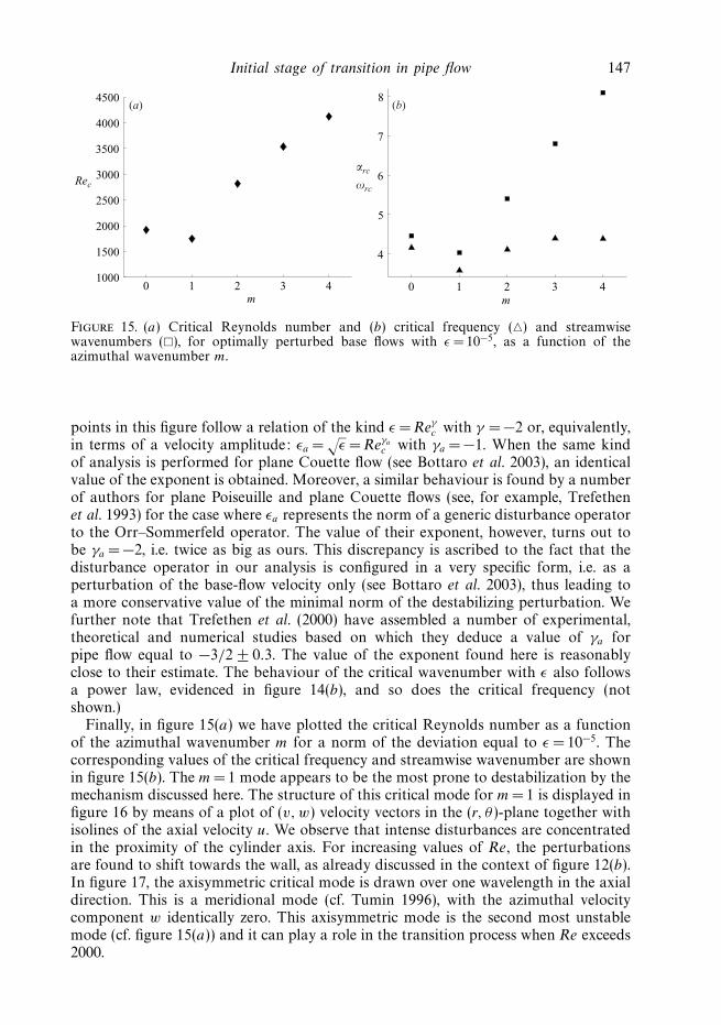
Figure 15. (a) Critical Reynolds number and (b) critical frequency (�) and streamwisewavenumbers (�), for optimally perturbed base flows with ε = 10−5, as a function of theazimuthal wavenumber m.
points in this figure follow a relation of the kind ε = Reγc with γ = −2 or, equivalently,
in terms of a velocity amplitude: εa =√
ε =Reγa
c with γa = −1. When the same kindof analysis is performed for plane Couette flow (see Bottaro et al. 2003), an identicalvalue of the exponent is obtained. Moreover, a similar behaviour is found by a numberof authors for plane Poiseuille and plane Couette flows (see, for example, Trefethenet al. 1993) for the case where εa represents the norm of a generic disturbance operatorto the Orr–Sommerfeld operator. The value of their exponent, however, turns out tobe γa = −2, i.e. twice as big as ours. This discrepancy is ascribed to the fact that thedisturbance operator in our analysis is configured in a very specific form, i.e. as aperturbation of the base-flow velocity only (see Bottaro et al. 2003), thus leading toa more conservative value of the minimal norm of the destabilizing perturbation. Wefurther note that Trefethen et al. (2000) have assembled a number of experimental,theoretical and numerical studies based on which they deduce a value of γa forpipe flow equal to −3/2 ± 0.3. The value of the exponent found here is reasonablyclose to their estimate. The behaviour of the critical wavenumber with ε also followsa power law, evidenced in figure 14(b), and so does the critical frequency (notshown.)
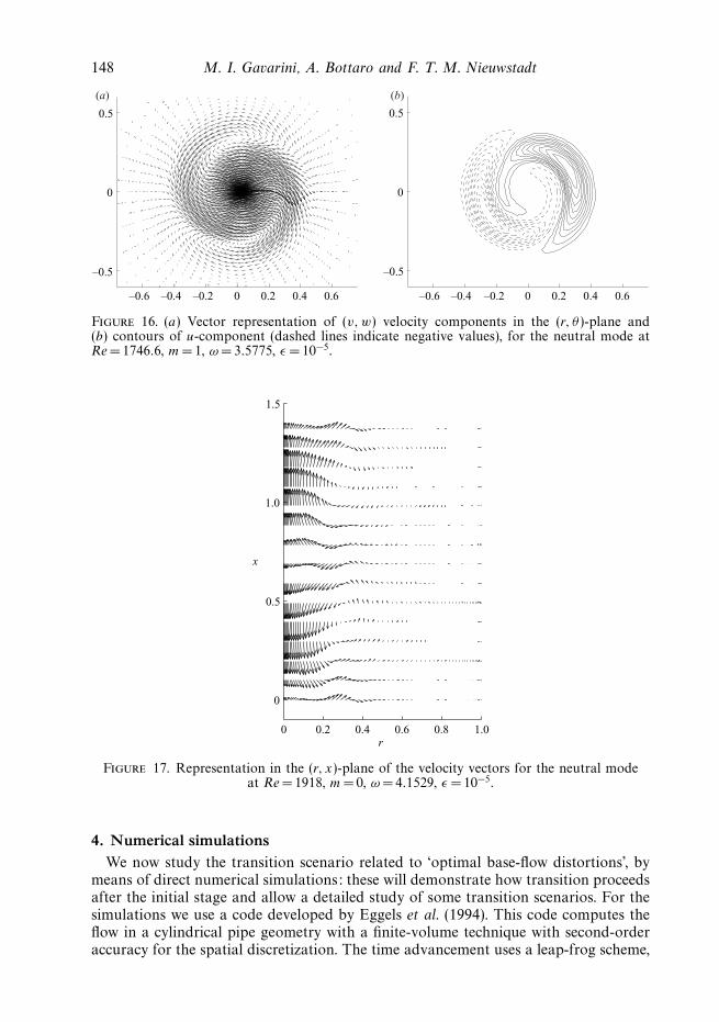
Finally, in figure 15(a) we have plotted the critical Reynolds number as a functionof the azimuthal wavenumber m for a norm of the deviation equal to ε = 10−5. Thecorresponding values of the critical frequency and streamwise wavenumber are shownin figure 15(b). The m =1 mode appears to be the most prone to destabilization by themechanism discussed here. The structure of this critical mode for m =1 is displayed infigure 16 by means of a plot of (v, w) velocity vectors in the (r, θ)-plane together withisolines of the axial velocity u. We observe that intense disturbances are concentratedin the proximity of the cylinder axis. For increasing values of Re, the perturbationsare found to shift towards the wall, as already discussed in the context of figure 12(b).In figure 17, the axisymmetric critical mode is drawn over one wavelength in the axialdirection. This is a meridional mode (cf. Tumin 1996), with the azimuthal velocitycomponent w identically zero. This axisymmetric mode is the second most unstablemode (cf. figure 15(a)) and it can play a role in the transition process when Re exceeds2000.
148 M. I. Gavarini, A. Bottaro and F. T. M. Nieuwstadt
–0.6 –0.4 –0.2 0 0.2 0.4 0.6
–0.5
0
0.5
–0.6 –0.4 –0.2 0 0.2 0.4 0.6
–0.5
0
0.5
(a) (b)
Figure 16. (a) Vector representation of (v,w) velocity components in the (r, θ )-plane and(b) contours of u-component (dashed lines indicate negative values), for the neutral mode atRe= 1746.6, m= 1, ω = 3.5775, ε =10−5.
0 0.2 0.4 0.6 0.8 1.0
0
0.5
1.0
1.5
r
x
Figure 17. Representation in the (r, x)-plane of the velocity vectors for the neutral modeat Re= 1918, m= 0, ω = 4.1529, ε =10−5.
4. Numerical simulationsWe now study the transition scenario related to ‘optimal base-flow distortions’, by
means of direct numerical simulations: these will demonstrate how transition proceedsafter the initial stage and allow a detailed study of some transition scenarios. For thesimulations we use a code developed by Eggels et al. (1994). This code computes theflow in a cylindrical pipe geometry with a finite-volume technique with second-orderaccuracy for the spatial discretization. The time advancement uses a leap-frog scheme,
Initial stage of transition in pipe flow 149
with second-order accuracy for the discretization of the advective terms and a forwardEuler scheme over two time steps for the diffusive terms. For further details, refer toEggels et al. (1994). The code has been extensively checked by reproducing the resultsobtained by Ma et al. (1999), who have used a spectral code. The agreement is foundto be excellent and this gives us the necessary confidence that the transition processcan be adequately simulated with the present second-order finite-volume code.
After these tests, the code has been modified to simulate the spatial developmentof the disturbance velocity v = (u, v, w) evolving on top of a given axisymmetric,not necessarily parabolic, base flow velocity distribution U (r). The resulting set ofequations reads:
∂u
∂x+
1
r
∂ (rv)
∂r+
1
r
∂w
∂θ= 0, (4.1a)
∂u
∂t+ (U + u)
∂u
∂x+ v
∂u
∂r+ v
dU
dr+ w
1
r
∂u
∂θ= −∂p
∂x+
1
Re∇2u, (4.1b)
∂v
∂t+ (U + u)
∂v
∂x+ v
∂v
∂r+ w
1
r
∂v
∂θ= −∂p
∂r+
1
Re
(∇2v − v
r2− 2
r2
∂w
∂θ
), (4.1c)
∂w
∂t+ (U + u)
∂w
∂x+ v
∂w
∂r+ w
1
r
∂w
∂θ= −1
r
∂p
∂θ+
1
Re
(∇2w − w
r2+
2
r2
∂v
∂θ
), (4.1d )
where ∇2 is again given by (2.3).In these equations, no additional forcing term is needed to produce and maintain the
base flow U (r). At the end of the computational domain, a fringe-region technique isimplemented, following closely the method proposed by Lundbladh et al. (1994), whoapply this method in their spectral code to combine the spatial evolution of the flowwith periodic boundary conditions in the streamwise direction. In our case, the fringeregion is used to gradually damp the disturbances flowing out of the physical domainwith minimal reflection. This proves to be necessary to eliminate numerical wigglesoriginating at the outflow boundary. At the inflow boundary, the unstable mode ofthe optimally perturbed base flow U (r) is imposed with a prescribed amplitude.
The results of the simulations are analysed in terms of the kinetic energy of thedisturbance velocity split up in its individual Fourier components according to:
E(m,n)dis (x) =
∑j=±m
∑k=±n
1
T
τ+T∫τ
2π∫0
1∫0
1
2
∣∣v (r, x; j, k) ei(j θ−k ωt)∣∣2 r dr dθ dt. (4.2)
Here, T =2π/ω and τ is an arbitrary starting time, subject to the condition that theasymptotic temporal state has been reached. The number pair (m, n) indicates theharmonics, where m is the wavenumber in the angular direction and n the multipleof the non-dimensional frequency ω. At the inflow, a disturbance is prescribed witha given value of (m, n), which is called the fundamental mode. During the transitionprocess, wavenumbers will be excited by nonlinear triad interactions that are multiplesof the fundamental mode and these are called higher harmonics. Equation (4.2) showsthat the spectral energy for each (m, n) is computed as the sum over the modes(±m, ±n).
4.1. Mode m = ± 1 and n= ± 1 as inflow condition
We consider, in this case, the unstable mode illustrated in figure 8, which refers tothe optimally modified base flow shown in figure 5. The parameters for this flow are
150 M. I. Gavarini, A. Bottaro and F. T. M. Nieuwstadt
0 20 40 60 80 100 12010–10
10–8
10–6
10–4
10–2
100
x
E (m,n)dis
(2,0) (0,0)
(1,1)
(4,0)
(3,1)
(6,0) (5,1)
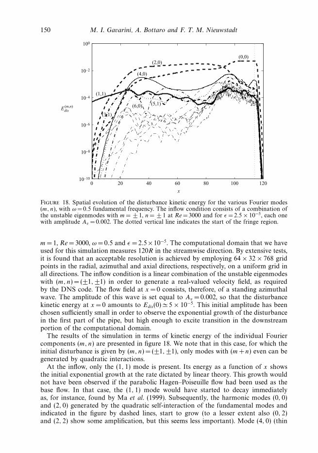
Figure 18. Spatial evolution of the disturbance kinetic energy for the various Fourier modes(m, n), with ω = 0.5 fundamental frequency. The inflow condition consists of a combination ofthe unstable eigenmodes with m= ± 1, n= ± 1 at Re= 3000 and for ε =2.5 × 10⁻⁵, each onewith amplitude Av = 0.002. The dotted vertical line indicates the start of the fringe region.
m =1, Re = 3000, ω = 0.5 and ε = 2.5×10⁻⁵. The computational domain that we haveused for this simulation measures 120R in the streamwise direction. By extensive tests,it is found that an acceptable resolution is achieved by employing 64 × 32 × 768 gridpoints in the radial, azimuthal and axial directions, respectively, on a uniform grid inall directions. The inflow condition is a linear combination of the unstable eigenmodeswith (m, n) = (±1, ±1) in order to generate a real-valued velocity field, as requiredby the DNS code. The flow field at x = 0 consists, therefore, of a standing azimuthalwave. The amplitude of this wave is set equal to Av =0.002, so that the disturbancekinetic energy at x = 0 amounts to Edis(0) � 5 × 10⁻⁵. This initial amplitude has beenchosen sufficiently small in order to observe the exponential growth of the disturbancein the first part of the pipe, but high enough to excite transition in the downstreamportion of the computational domain.
The results of the simulation in terms of kinetic energy of the individual Fouriercomponents (m, n) are presented in figure 18. We note that in this case, for which theinitial disturbance is given by (m, n) = (±1, ±1), only modes with (m+n) even can begenerated by quadratic interactions.
At the inflow, only the (1, 1) mode is present. Its energy as a function of x showsthe initial exponential growth at the rate dictated by linear theory. This growth wouldnot have been observed if the parabolic Hagen–Poiseuille flow had been used as thebase flow. In that case, the (1, 1) mode would have started to decay immediatelyas, for instance, found by Ma et al. (1999). Subsequently, the harmonic modes (0, 0)and (2, 0) generated by the quadratic self-interaction of the fundamental modes andindicated in the figure by dashed lines, start to grow (to a lesser extent also (0, 2)and (2, 2) show some amplification, but this seems less important). Mode (4, 0) (thin
Initial stage of transition in pipe flow 151
x
r*θ
25 50 75 100
1
2
3
4
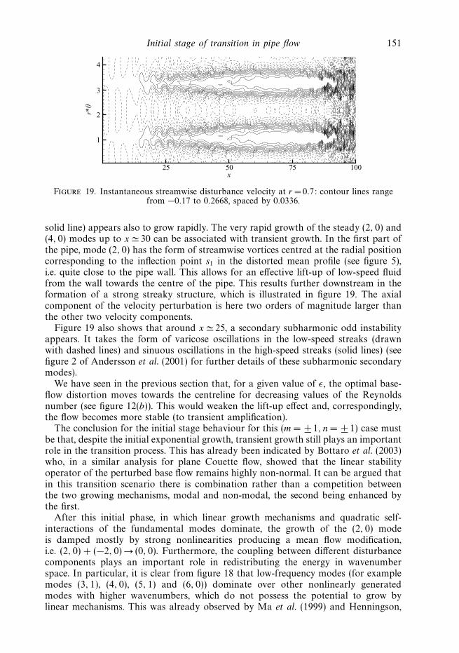
Figure 19. Instantaneous streamwise disturbance velocity at r = 0.7: contour lines rangefrom −0.17 to 0.2668, spaced by 0.0336.
solid line) appears also to grow rapidly. The very rapid growth of the steady (2, 0) and(4, 0) modes up to x � 30 can be associated with transient growth. In the first part ofthe pipe, mode (2, 0) has the form of streamwise vortices centred at the radial positioncorresponding to the inflection point s1 in the distorted mean profile (see figure 5),i.e. quite close to the pipe wall. This allows for an effective lift-up of low-speed fluidfrom the wall towards the centre of the pipe. This results further downstream in theformation of a strong streaky structure, which is illustrated in figure 19. The axialcomponent of the velocity perturbation is here two orders of magnitude larger thanthe other two velocity components.
Figure 19 also shows that around x � 25, a secondary subharmonic odd instabilityappears. It takes the form of varicose oscillations in the low-speed streaks (drawnwith dashed lines) and sinuous oscillations in the high-speed streaks (solid lines) (seefigure 2 of Andersson et al. (2001) for further details of these subharmonic secondarymodes).
We have seen in the previous section that, for a given value of ε, the optimal base-flow distortion moves towards the centreline for decreasing values of the Reynoldsnumber (see figure 12(b)). This would weaken the lift-up effect and, correspondingly,the flow becomes more stable (to transient amplification).
The conclusion for the initial stage behaviour for this (m = ± 1, n = ± 1) case mustbe that, despite the initial exponential growth, transient growth still plays an importantrole in the transition process. This has already been indicated by Bottaro et al. (2003)who, in a similar analysis for plane Couette flow, showed that the linear stabilityoperator of the perturbed base flow remains highly non-normal. It can be argued thatin this transition scenario there is combination rather than a competition betweenthe two growing mechanisms, modal and non-modal, the second being enhanced bythe first.
After this initial phase, in which linear growth mechanisms and quadratic self-interactions of the fundamental modes dominate, the growth of the (2, 0) modeis damped mostly by strong nonlinearities producing a mean flow modification,i.e. (2, 0) + (−2, 0) → (0, 0). Furthermore, the coupling between different disturbancecomponents plays an important role in redistributing the energy in wavenumberspace. In particular, it is clear from figure 18 that low-frequency modes (for examplemodes (3, 1), (4, 0), (5, 1) and (6, 0)) dominate over other nonlinearly generatedmodes with higher wavenumbers, which do not possess the potential to grow bylinear mechanisms. This was already observed by Ma et al. (1999) and Henningson,
152 M. I. Gavarini, A. Bottaro and F. T. M. Nieuwstadt
Lundbladh & Johansson (1993), who speak, respectively, of an m-cascade in Hagen–Poiseuille flow or a β-cascade in plane Poiseuille flow, in which the disturbanceenergy is mainly transferred through a route with increasing azimuthal or spanwisewavenumber.
Beyond the downstream position where the energy of the (2, 0) mode reaches apeak, i.e. at x � 75, a second phase of rapid growth of higher-order modes, i.e. modeswith higher harmonics of ω, is responsible for the final breakdown to turbulence.
A sequence of events comparable with the case described above was also foundby Berlin et al. (1994) for a boundary-layer flow, in which transition was initiatedby a pair of oblique waves, which could grow transiently in the initial stage andwhose quadratic interaction resulted in the generation of streamwise vortices. Thesevortices, in turn, produced streaks by the lift-up mechanism, eventually bringing theflow to transition via a secondary instability of the streaky flow. Our case, however,differs from that of Berlin et al. (1994), because our process starts with the primaryinstability of the modified base flow, i.e. the initial energy in the streamwise vorticesis fed by the exponential growth of the unstable mode.
In a simulation with the amplitude of each unstable mode at the inflow equal toAv = 0.001, i.e. for Edis(0) � 1.25 × 10⁻⁵, the second phase of rapid growth of thehigher-order frequency harmonics and the ensuing transition to turbulence did notoccur. Instead, a decay of the streaks after the peak in the energy of the (2, 0) modewas observed. Therefore, in this scenario starting with the exponential growth ofsmall disturbances on a modified base flow, which can directly generate streamwisevortices and streaks, the essential feature, which determines whether transition occursor not, is the final amplitude of the streaks. This amplitude must reach a thresholdvalue in order to force the final breakdown. It can thus be stated that the wholetransition process in this case is dominated by the evolution and breakdown of thelarge-amplitude streaks, as shown in figure 19. Therefore, this scenario could gounder the classification of oblique transition (see Schmid & Henningson 2001), theonly difference being that here the infinitesimal oblique (in our case actually helical)waves can initially grow exponentially. The subsequent series of events becomes thenqualitatively similar to that observed in numerical simulations initiated by the non-modal amplification of optimal initial vortices (see O’Sullivan & Breuer 1994 b; Maet al. 1999).
4.2. Mode m =0 and n= ± 2 as inflow condition
Our analysis of optimal base-flow deviations has also shown that axisymmetricdisturbances can experience exponential amplification. Let us consider this case witha superposition of modes (0, ±2) as initial condition. For such a disturbance, quadraticself-interaction cannot produce modes such as (2, 0), which, as we have seen in theprevious section, play a central role in the oblique transition process. Therefore, weexpect, in this case, a different transition scenario and its elucidation is the objectiveof our second numerical simulation.
The computational domain used in this second case measures 80R in the streamwisedirection, with a resolution of 64 × 32 × 640 grid points in the radial, azimuthal andaxial directions, respectively. We use the optimally modified base flow at Re= 3000,and ε = 2.5 × 10⁻⁵, which destabilizes an axisymmetric disturbance with frequencyω = 1 (note that ω = 0.5 is still used as the fundamental frequency in the Fourierdecomposition). Stability theory predicts a growth rate of the unstable mode equal to−αi =0.07955. The inflow condition consists of a combination of the (0, ±2) Fouriermodes to obtain a real inflow velocity field and the amplitude was chosen equal to
Initial stage of transition in pipe flow 153
0 10 20 30 40 50 60 70 8010–16
10–14
10–12
10–10
10–8
10–6
10–4
10–2
100
x
(0,2)
(0,4)
(0,0)
(2,1)
(3,1)
Edis(m,n)
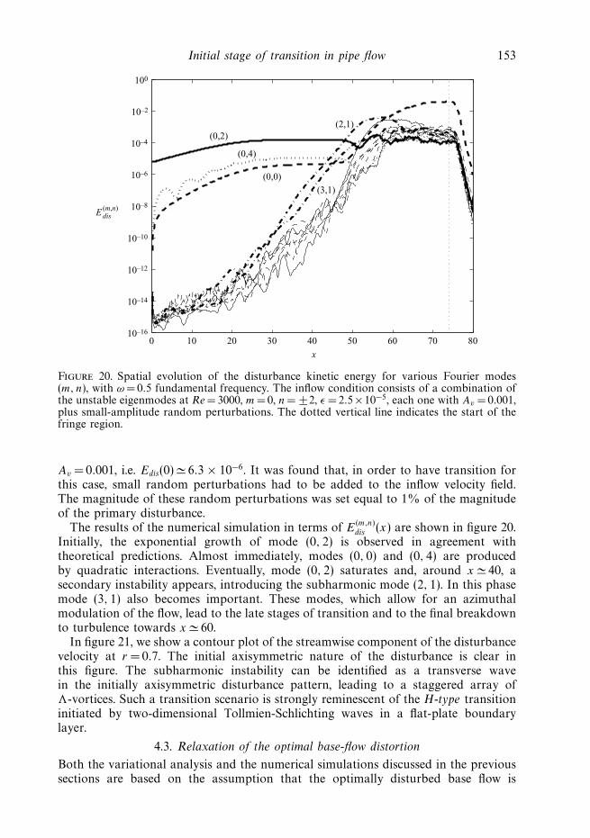
Figure 20. Spatial evolution of the disturbance kinetic energy for various Fourier modes(m, n), with ω = 0.5 fundamental frequency. The inflow condition consists of a combination ofthe unstable eigenmodes at Re= 3000, m= 0, n= ±2, ε =2.5×10⁻⁵, each one with Av = 0.001,plus small-amplitude random perturbations. The dotted vertical line indicates the start of thefringe region.
Av = 0.001, i.e. Edis(0) � 6.3 × 10⁻⁶. It was found that, in order to have transition forthis case, small random perturbations had to be added to the inflow velocity field.The magnitude of these random perturbations was set equal to 1% of the magnitudeof the primary disturbance.
The results of the numerical simulation in terms of E(m,n)dis (x) are shown in figure 20.
Initially, the exponential growth of mode (0, 2) is observed in agreement withtheoretical predictions. Almost immediately, modes (0, 0) and (0, 4) are producedby quadratic interactions. Eventually, mode (0, 2) saturates and, around x � 40, asecondary instability appears, introducing the subharmonic mode (2, 1). In this phasemode (3, 1) also becomes important. These modes, which allow for an azimuthalmodulation of the flow, lead to the late stages of transition and to the final breakdownto turbulence towards x � 60.
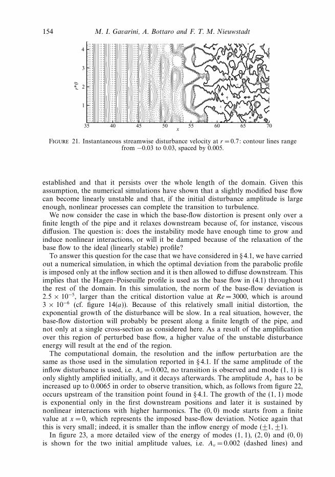
In figure 21, we show a contour plot of the streamwise component of the disturbancevelocity at r = 0.7. The initial axisymmetric nature of the disturbance is clear inthis figure. The subharmonic instability can be identified as a transverse wavein the initially axisymmetric disturbance pattern, leading to a staggered array of�-vortices. Such a transition scenario is strongly reminescent of the H-type transitioninitiated by two-dimensional Tollmien-Schlichting waves in a flat-plate boundarylayer.
4.3. Relaxation of the optimal base-flow distortion
Both the variational analysis and the numerical simulations discussed in the previoussections are based on the assumption that the optimally disturbed base flow is
154 M. I. Gavarini, A. Bottaro and F. T. M. Nieuwstadt
x
r*θ
35 40 45 50 55 60 65 70
1
2
3
4
Figure 21. Instantaneous streamwise disturbance velocity at r = 0.7: contour lines rangefrom −0.03 to 0.03, spaced by 0.005.
established and that it persists over the whole length of the domain. Given thisassumption, the numerical simulations have shown that a slightly modified base flowcan become linearly unstable and that, if the initial disturbance amplitude is largeenough, nonlinear processes can complete the transition to turbulence.
We now consider the case in which the base-flow distortion is present only over afinite length of the pipe and it relaxes downstream because of, for instance, viscousdiffusion. The question is: does the instability mode have enough time to grow andinduce nonlinear interactions, or will it be damped because of the relaxation of thebase flow to the ideal (linearly stable) profile?
To answer this question for the case that we have considered in § 4.1, we have carriedout a numerical simulation, in which the optimal deviation from the parabolic profileis imposed only at the inflow section and it is then allowed to diffuse downstream. Thisimplies that the Hagen–Poiseuille profile is used as the base flow in (4.1) throughoutthe rest of the domain. In this simulation, the norm of the base-flow deviation is2.5 × 10−5, larger than the critical distortion value at Re = 3000, which is around3 × 10−6 (cf. figure 14(a)). Because of this relatively small initial distortion, theexponential growth of the disturbance will be slow. In a real situation, however, thebase-flow distortion will probably be present along a finite length of the pipe, andnot only at a single cross-section as considered here. As a result of the amplificationover this region of perturbed base flow, a higher value of the unstable disturbanceenergy will result at the end of the region.
The computational domain, the resolution and the inflow perturbation are thesame as those used in the simulation reported in § 4.1. If the same amplitude of theinflow disturbance is used, i.e. Av =0.002, no transition is observed and mode (1, 1) isonly slightly amplified initially, and it decays afterwards. The amplitude Av has to beincreased up to 0.0065 in order to observe transition, which, as follows from figure 22,occurs upstream of the transition point found in § 4.1. The growth of the (1, 1) modeis exponential only in the first downstream positions and later it is sustained bynonlinear interactions with higher harmonics. The (0, 0) mode starts from a finitevalue at x = 0, which represents the imposed base-flow deviation. Notice again thatthis is very small; indeed, it is smaller than the inflow energy of mode (±1, ±1).
In figure 23, a more detailed view of the energy of modes (1, 1), (2, 0) and (0, 0)is shown for the two initial amplitude values, i.e. Av = 0.002 (dashed lines) and
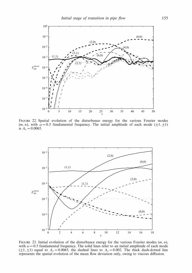
Initial stage of transition in pipe flow 155
0 5 10 15 20 25 30 35 40 45 5010–8
10–7
10–6
10–5
10–4
10–3
10–2
10–1
100
Edis(m,n)
(0,0)
(2,0)
(1,1) (3,1)
(6,0)
(5,1)
(4,0)
x
Figure 22. Spatial evolution of the disturbance energy for the various Fourier modes(m, n), with ω = 0.5 fundamental frequency. The initial amplitude of each mode (±1, ±1)is Av = 0.0065.
0 2 4 6 8 10 12 14 16 1810–7
10–6
10–5
10–4
10–3
10–2
(1,1)
(2,0)
(0,0)
(1,1)
(2,0)
(0,0)
Edis(m,n)
x
Figure 23. Initial evolution of the disturbance energy for the various Fourier modes (m, n),with ω = 0.5 fundamental frequency. The solid lines refer to an initial amplitude of each mode(±1, ±1) equal to Av = 0.0065, the dashed lines to Av = 0.002. The thick dash-dotted linerepresents the spatial evolution of the mean flow deviation only, owing to viscous diffusion.
156 M. I. Gavarini, A. Bottaro and F. T. M. Nieuwstadt
Av = 0.0065 (solid lines). In the figure we also show the evolution of the energyof the mean flow distortion alone (thick dash-dotted line), and its threshold valueat Re = 3000 (dotted horizontal line), i.e. the value below which the exponentialgrowth of the (1, 1) mode is no longer sustained. The mean flow distortion isobserved to decay rapidly at this relatively low value of the Reynolds number.When its energy goes below the threshold, the (2, 0) mode for the case with thehigher value of Av has an energy comparable to that of mode (1, 1). Therefore,the streamwise vortices and the resulting streaks are strong enough to influence,by means of nonlinear interactions with the (3, 1) mode (not shown), the evolutionof the (1, 1) mode, which thus can grow further. For the lower value of Av , whenthe threshold is crossed at x close to 4, the (2, 0) mode is still very weak so thatthe growth of the (1, 1) mode cannot be sustained either by linear or by nonlinearmechanisms and consequently the initial perturbation decays. Therefore, also inthis case we can conclude that the occurrence of transition is influenced by theamplitude of the streaks downstream of the position where the distortion has beenintroduced.
A similar numerical simulation has also been performed for the axisymmetricdisturbance analysed in § 4.2. When the base-flow perturbation is applied only at theinflow, we find that, owing to the rapid diffusion of the optimal base-flow distortion,the exponential growth of the axisymmetric unstable mode is confined to a distanceof only a few pipe diameters. From that point on, any further growth of the initialperturbation mode (0, 2) and of the nonlinearly generated modes (0, 0) and (0, 4)is excluded, since non-modal effects are very weak for axisymmetric disturbances(see Schmid & Henningson 2001). Even an increase in the value of the initialdisturbance amplitude up to Av = 0.01 was not sufficient to provoke transition in theflow.
To find the reason for this failure to produce transition we consider the total energyof the disturbance calculated as the sum over all modes m and n, which reads:
Edis(x) =∑
m
∑n
E(m,n)dis (x).
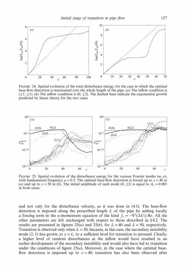
The behaviour of Edis as a function of x for the cases considered in § § 4.1 and 4.2,where the base-flow distortion was imposed over the whole length of the pipe, ispresented in figure 24, in which we also show the exponential growth of Edis as aresult of linear theory.
For the case with the (±1, ±1) inflow condition, the nonlinearity is clearlydestabilizing, resulting in a faster than exponential growth of the energy, implyingthat transition occurs via a subcritical bifurcation from the base state (Barkley &Tuckerman 1999). On the other hand, for the (0, ±2) inflow condition, the nonlinearityclearly saturates the linear instability resulting in a lower than exponential growth ofthe energy and in the supercritical nature of the bifurcation.
Therefore, we conclude that for the latter scenario to be observed, the optimalbase-flow deviation must persist over a finite length of the pipe and the inducedgrowth (i.e. the norm of the deviation itself) must be strong enough for the late stageto set in before the base-flow deviation is smeared out by viscosity. This is confirmedby two additional simulations, in which the optimal base-flow distortion is forcedalong a finite length of the pipe extending from the inflow section up to x = 40 andx = 50, respectively, and it is then allowed to relax further downstream. For thesesimulations, the Navier–Stokes equations are solved for the complete velocity field
Initial stage of transition in pipe flow 157
20 40 60 80 1000
2
4
6
8
log(
Edi
s/E
dis(
0))
log(
Edi
s/E
dis(
0))
x10 20 30 40 50 60 700
2
4
6
8
10
x
(a) (b)
Figure 24. Spatial evolution of the total disturbance energy, for the case in which the optimalbase-flow distortion is maintained over the whole length of the pipe. (a) The inflow condition is(±1, ±1). (b) The inflow condition is (0, ±2). The dashed lines indicate the exponential growthpredicted by linear theory for the two cases.
0 20 40 6010–15
10–10
10–5
100
x x
Edis(m,n)
10–15
10–10
10–5
100
Edis(m,n)
(0,0) (0,2)
(0,4)
(2,1)
0 20 40 60
(0,0) (0,2)
(0,4)
(2,1) (a) (b)
Figure 25. Spatial evolution of the disturbance energy for the various Fourier modes (m, n),with fundamental frequency ω = 0.5. The optimal base-flow distortion is forced up to x = 40 in(a) and up to x = 50 in (b). The initial amplitude of each mode (0, ±2) is equal to Av = 0.001in both cases.
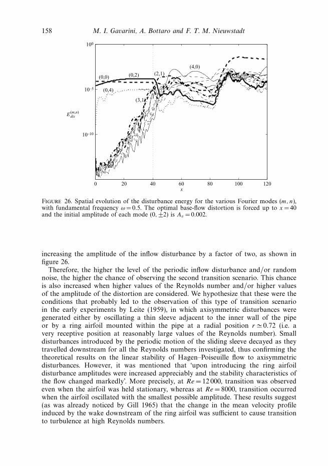
and not only for the disturbance velocity, as it was done in (4.1). The base-flowdistortion is imposed along the prescribed length L of the pipe by adding locallya forcing term in the u-momentum equation of the kind fx = −∇2(U )/Re. All theother parameters are left unchanged with respect to those described in § 4.2. Theresults are presented in figures 25(a) and 25(b), for L = 40 and L = 50, respectively.Transition is observed only when L = 50, because, in this case, the secondary instabilitymode (2, 1) has grown, at x = L, to a sufficient level for transition to proceed. Clearly,a higher level of random disturbances at the inflow would have resulted in anearlier development of the secondary instability and would also have led to transitionunder the conditions of figure 25(a). Moreover, in the case where the optimal base-flow distortion is imposed up to x = 40, transition has also been observed after
158 M. I. Gavarini, A. Bottaro and F. T. M. Nieuwstadt
0 20 40 60 80 100 120
10–10
10–5
100
x
Edis(m,n)
(0,2) (0,0)
(0,4)
(2,1) (4,0)
(3,1)
Figure 26. Spatial evolution of the disturbance energy for the various Fourier modes (m, n),with fundamental frequency ω = 0.5. The optimal base-flow distortion is forced up to x = 40and the initial amplitude of each mode (0, ±2) is Av = 0.002.
increasing the amplitude of the inflow disturbance by a factor of two, as shown infigure 26.
Therefore, the higher the level of the periodic inflow disturbance and/or randomnoise, the higher the chance of observing the second transition scenario. This chanceis also increased when higher values of the Reynolds number and/or higher valuesof the amplitude of the distortion are considered. We hypothesize that these were theconditions that probably led to the observation of this type of transition scenarioin the early experiments by Leite (1959), in which axisymmetric disturbances weregenerated either by oscillating a thin sleeve adjacent to the inner wall of the pipeor by a ring airfoil mounted within the pipe at a radial position r � 0.72 (i.e. avery receptive position at reasonably large values of the Reynolds number). Smalldisturbances introduced by the periodic motion of the sliding sleeve decayed as theytravelled downstream for all the Reynolds numbers investigated, thus confirming thetheoretical results on the linear stability of Hagen–Poiseuille flow to axisymmetricdisturbances. However, it was mentioned that ‘upon introducing the ring airfoildisturbance amplitudes were increased appreciably and the stability characteristics ofthe flow changed markedly’. More precisely, at Re = 12 000, transition was observedeven when the airfoil was held stationary, whereas at Re = 8000, transition occurredwhen the airfoil oscillated with the smallest possible amplitude. These results suggest(as was already noticed by Gill 1965) that the change in the mean velocity profileinduced by the wake downstream of the ring airfoil was sufficient to cause transitionto turbulence at high Reynolds numbers.
Initial stage of transition in pipe flow 159
4.4. Discussion
Bottin et al. (1998) have given experimental evidence for the effect that small base-flow distortions have on the stability characteristics of subcritical shear flows. Theyfound that finite-amplitude solutions, in the form of streamwise vortices, bifurcatesubcritically from a plane Couette flow slightly modified (and destabilized) by a thinspanwise wire in the zero-velocity plane (i.e. at the position that returns the greatesteffects in the destabilization of the mean flow, see Gill 1965; Bottaro et al. 2003). Theyalso found that this streamwise-streak state still bifurcates when the diameter of thewire is gradually decreased to zero, i.e. when the distortion of the mean speed vanishes.Moreover, the streamwise extent of the streaks is much larger than the region wherethe profile is significantly modified by the presence of the wire, suggesting that theflow has switched to a new state that has little to do with the modified basic state asresults also from our calculations. These results have been confirmed by numericalsimulations performed by Barkley & Tuckerman (1999), who also indicated that smallgeometric perturbations destabilize plane Couette flow via a subcritical instabilityand that the bifurcating solution is a three-dimensional flow with streamwisevortices.
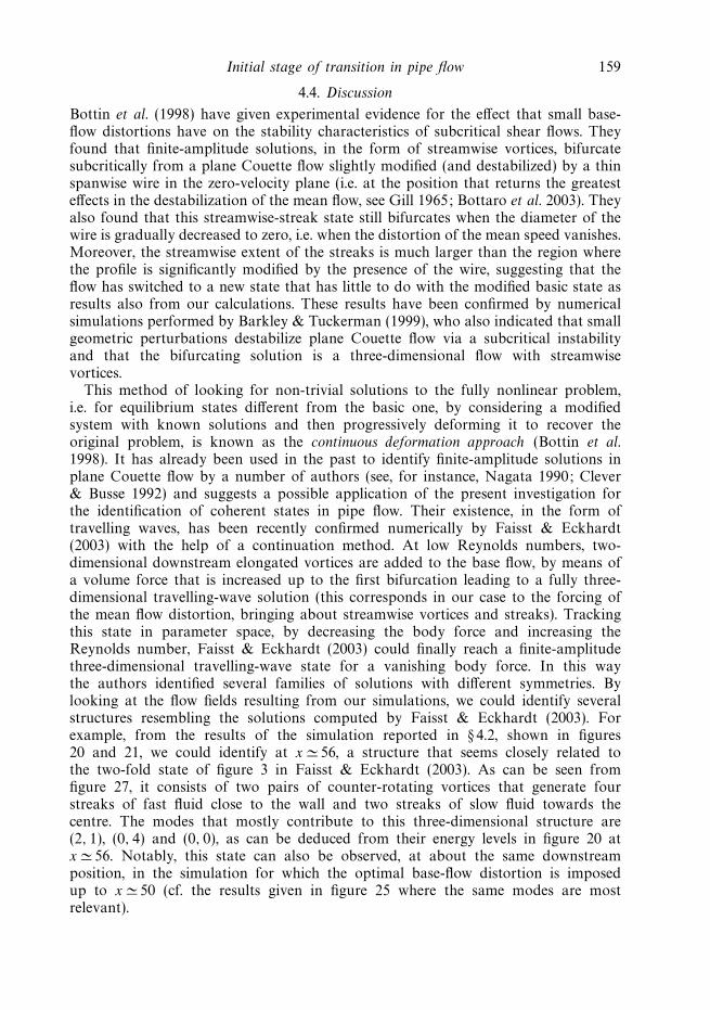
This method of looking for non-trivial solutions to the fully nonlinear problem,i.e. for equilibrium states different from the basic one, by considering a modifiedsystem with known solutions and then progressively deforming it to recover theoriginal problem, is known as the continuous deformation approach (Bottin et al.1998). It has already been used in the past to identify finite-amplitude solutions inplane Couette flow by a number of authors (see, for instance, Nagata 1990; Clever& Busse 1992) and suggests a possible application of the present investigation forthe identification of coherent states in pipe flow. Their existence, in the form oftravelling waves, has been recently confirmed numerically by Faisst & Eckhardt(2003) with the help of a continuation method. At low Reynolds numbers, two-dimensional downstream elongated vortices are added to the base flow, by means ofa volume force that is increased up to the first bifurcation leading to a fully three-dimensional travelling-wave solution (this corresponds in our case to the forcing ofthe mean flow distortion, bringing about streamwise vortices and streaks). Trackingthis state in parameter space, by decreasing the body force and increasing theReynolds number, Faisst & Eckhardt (2003) could finally reach a finite-amplitudethree-dimensional travelling-wave state for a vanishing body force. In this waythe authors identified several families of solutions with different symmetries. Bylooking at the flow fields resulting from our simulations, we could identify severalstructures resembling the solutions computed by Faisst & Eckhardt (2003). Forexample, from the results of the simulation reported in § 4.2, shown in figures20 and 21, we could identify at x � 56, a structure that seems closely related tothe two-fold state of figure 3 in Faisst & Eckhardt (2003). As can be seen fromfigure 27, it consists of two pairs of counter-rotating vortices that generate fourstreaks of fast fluid close to the wall and two streaks of slow fluid towards thecentre. The modes that mostly contribute to this three-dimensional structure are(2, 1), (0, 4) and (0, 0), as can be deduced from their energy levels in figure 20 atx � 56. Notably, this state can also be observed, at about the same downstreamposition, in the simulation for which the optimal base-flow distortion is imposedup to x � 50 (cf. the results given in figure 25 where the same modes are mostrelevant).
160 M. I. Gavarini, A. Bottaro and F. T. M. Nieuwstadt
Figure 27. Instantaneous velocity field corresponding to the simulation shown in figures 20and 21 at x � 56. The contour lines range from −0.12 to 0.12, spaced by 0.016; the vectorsrepresent the secondary velocity in the pipe cross-section.
5. ConclusionsThe present theoretical/computational investigation originates from experimental
observations which highlight the considerable importance of base-flow distortionsin the transition process of cylindrical pipe flow (e.g. Eliahou et al. 1998). Againstthis background, we have explored the spatial growth of infinitesimal disturbancesdeveloping on top of a distorted axially invariant pipe flow, which consists of theparabolic Hagen–Poiseuille modified by a small axisymmetric distortion. In actualexperiments, such deviations from the theoretical velocity distribution may occurbecause of surface roughness, external volume forces, flow inhomogeneities, and soon. The limitation of the present study is that only axisymmetric axially invariantbase-flow deformations have been considered.
To investigate the sensitivity to these base-flow variations, we have analysed theeigenvalues of the linearized Navier–Stokes operator and have identified the mostsensitive eigenmodes. They are found to coincide with the eigenvalues recognised byTumin (1996) as the most ‘receptive’ to periodic blowing and suction through a slot atthe wall. With these ‘sensitive’ eigenvalues as point of departure, we have computedby means of a variational technique the so-called optimal base flow deviations forHagen–Poiseuille flow, i.e. those distortions which maximally destabilize the flow. Asa result, we have found that base-flow deviations of very small norm are capable ofsupporting perturbations, which show exponential growth. These so-called optimaldeviations lead to inflection points in the base-flow profile suggesting an inviscid-typeinstability.
With the help of the same variational technique, we have then computed thedependence of the instability to parameters such as the Reynolds number, the
Initial stage of transition in pipe flow 161
azimuthal wavenumber and the frequency of the disturbances. The neutral curves,obtained for fixed values of the norm of the optimal base flow deviation ε, show thatstreamwise waves of shorter wavelength and higher frequencies are excited as ε isdecreased. If an experimentalist engaged in pipe-flow measurements could provide anestimate of the expected variance of the deviation on his axial velocity, results such asthose provided in figures 13(a) and 14(a) would indicate whether or not exponentialgrowth of infinitesimal perturbations could be expected in the experiments.
Further conclusions of the theory are that the mode m =1 is the most prone todestabilization by the mechanism described here and that the axisymmetric modem = 0 can also be excited at Reynolds numbers of the order of 2000. In order toverify these theoretical results, the two modes with m =1 and m =0 have been usedas initial conditions in direct numerical simulations to study possible transition paths.It is first noted that transition can be started by the amplification of either mode,provided its initial amplitude is sufficiently large and/or the base-flow distortion isstrong enough. For the case with m =1, transition is observed even when the distortionis allowed to diffuse immediately from x = 0 under the action of viscosity, while forthe case with m = 0, the base-flow distortion must be present for a finite length of thepipe.
The numerical simulations show also that the path of transition resulting from thegrowth of the axisymmetric mode is reminiscent of the subharmonic H -transition scen-ario of boundary layers, with the formation of staggered patterns of �-vortices. Onthe other hand, for the mode m = 1, the formation of streamwise elongated streaks isobserved, that break down through a secondary subharmonic instability. This latterscenario seems to be the counterpart of the oblique transition scenario of Berlin et al.(1994).
This paper has added but a brick to the building of a thorough comprehension ofpipe-flow transition, by concentrating on plausible effects that can occur when thevelocity distribution used as a reference in the initial linearization of the equations isnot exactly equal to the theoretical profile. Future work will be devoted to the studyof non-axisymmetric base-flow distortions, and to the optimal and robust control ofpipe-flow transition.
The authors wish to thank Dr B. J. Boersma and Dr M. Pourquie, for their helpwith the numerical simulations. M. I.G. initiated this work in Toulouse with thesupport of the EU under a Marie Curie Training Site Fellowship, contract numberHPMT-CT-2000-00079.
Appendix A. Non-zero elements of matrices C0, C1 and C2
C120 = 1,
C210 =
(m2 + 1)
r2− iωRe; C22
0 = ReU (r); C250 =
2im
r2,
C310 = −1
r; C35
0 = − im
r,
C410 =
U (r)
r− dU
dr; C42
0 = − 1
Re r; C43
0 = iω − m2
Re r2; C45
0 =imU (r)
r,
C460 = − im
Re r,
162 M. I. Gavarini, A. Bottaro and F. T. M. Nieuwstadt
C560 = 1,
C610 = −2im
r2; C64
0 =imRe
r; C65
0 = −iωRe +(m2 + 1)
r2; C66
0 = ReU (r),
C211 = −1
r; C24
1 = Re,
C311 = −1,
C411 = U (r); C42
1 = − 1
Re; C43
1 =1
Re r,
C651 = −1
r,
C212 = −1; C43
2 =1
Re; C65
2 = − 1.
Appendix B. Generalized Rayleigh and Fjørtoft theorems for inviscid flows in acylindrical pipe geometry
In this Appendix, we shall briefly review the Rayleigh inflection point theorem andthe Fjørtoft criterion in cylindrical geometry (see also Batchelor & Gill 1962). Werestrict ourselves to axisymmetric disturbances and to their temporal evolution in theinviscid case, with a base flow given by U (r). The equation for the shape function Φ
of the streamfunction Ψ (x, r, t) =Φ(r) expiα(x−ct) is given by:(d2
dr2− 1
r
d
dr− α2
)Φ − r
(U ′
r
)′Φ
U − c= 0, (B 1)
where we have supposed that the temporal growth rate ci > 0 so that U − c �= 0. Theboundary conditions are: Φ/r and Φ ′/r bounded as r → 0, and Φ = 0 at r = 1. It isuseful to rewrite equation (B 1) as follows:[
rd
dr
(1
r
d
dr
)− α2
]Φ − r
(U ′
r
)′Φ
U − c= 0. (B 2)
Multiplying each term of this equation by the complex conjugate (Φ∗/r), andintegrating between r = 0 and r = 1, we obtain:[
Φ ′
r
]Φ∗|10 −
∫ 1
0
Φ ′Φ∗′
rdr − α2
∫ 1
0
ΦΦ∗
rdr −
∫ 1
0
(U ′
r
)′ΦΦ∗
U − cdr = 0. (B 3)
The first term is equal to zero on account of the boundary conditions, so that (B 3)can be rewritten as:∫ 1
0
(U ′
r
)′ |Φ|2U − c
dr = −∫ 1
0
1
r
[|Φ ′|2 + α2|Φ|2
]dr, (B 4)
with the right-hand side purely real. By taking the imaginary part of (B 4), we obtain,
ci
∫ 1
0
(U ′
r
)′ |Φ|2|U − c|2 dr = 0.
Since we have assumed that ci > 0, this integral can become zero only if (U ′/r)′
changes sign at least once in the open interval (0, 1). Hence, the necessary condition
Initial stage of transition in pipe flow 163
for instability is: (U ′
r
)′
= 0, (B 5)
which is a generalization to cylindrical coordinates of Rayleigh’s inflection-pointcriterion. The quantity U ′/r can be interpreted as the circulation, which shouldtherefore have a maximum somewhere in the flow for instability to be possible.
A stronger criterion of inviscid instability is provided by the Fjørtoft theorem,which can be derived by taking the real part of (B 4). This leads to:∫ 1
0
(U ′
r
)′U − cr
|U − c|2 |Φ|2dr = −∫ 1
0
1
r
[|Φ ′|2 +α2|Φ|2
]dr < 0.
If we now add to the left-hand side the term:
(cr − Us)
∫ 1
0
(U ′
r
)′ |Φ|2|U − c|2 dr = 0,
where Us = U (rs) is the velocity of the base flow calculated at the radial positionwhere (B 5) is satisfied, we obtain,∫ 1
0
(U ′
r
)′U − Us
|U − c|2 |Φ|2dr < 0, (B 6)
from which it follows that a necessary condition for instability is:(U ′
r
)′
(U − Us) < 0 (B 7)
somewhere in the flow field. Although (B 5) and (B 7) are rather straightforwardextensions of classical results for plane shear flows, we feel that it is useful to reportthem here since we have been unable to find (B 7) in the literature.
REFERENCES
Andersson, P., Brandt, L., Bottaro, A. & Henningson, D. S. 2001 On the breakdown of boundarylayer streaks. J. Fluid Mech. 428, 29–60.
Barkley, D. & Tuckerman, L. S. 1999 Stability analysis of perturbed plane Couette flow. Phys.Fluids A 5, 1187–1195.
Batchelor, G. K. & Gill, A. E. 1962 Analysis of the stability of axisymmetric jets. J. Fluid Mech.14, 529–551.
Bergstrom, L. 1992 Initial algebraic growth of small angular dependent disturbances in pipePoiseuille flow. Stud. Appl. Maths 87, 61–79.
Bergstrom, L. 1993 Optimal growth of small disturbances in pipe Poiseuille flow. Phys. Fluids A 5,2710–2720.
Berlin, S., Lundbladh, A. & Henningson, D. S. 1994 Spatial simulations of oblique transition ina boundary layer. Phys. Fluids 6, 1949–1951.
Berlin, S., Wiegel, M. & Henningson, D. S. 1999 Numerical and experimental investigations ofoblique boundary layer transition. J. Fluid Mech. 393, 23–57.
Boberg, L. & Brosa, U. 1988 Onset of turbulence in a pipe. Z. Naturforsch. 43a, 697–726.
Bottaro, A., Corbett, P. & Luchini, P. 2003 The effect of base flow variation on flow stability.J. Fluid Mech. 476, 293–302.
Bottin, S., Dauchot, O., Daviaud, F. & Manneville, P. 1998 Experimental evidence of streamwisevortices as finite amplitude solutions in transitional plane Couette flow. Phys. Fluids 10,2597–2607.
164 M. I. Gavarini, A. Bottaro and F. T. M. Nieuwstadt
Clever, R. M. & Busse, F. H. 1992 Three dimensional convection in a horizontal fluid layersubjected to a constant shear. J. Fluid Mech. 234, 511–527.
Darbyshire, A. G. & Mullin, T. 1995 Transition to turbulence in constant mass-flux pipe flow.J. Fluid Mech. 289, 83–114.
Davey, A. 1978 On the stability of flow in an elliptic pipe which is nearly circular. J. Fluid Mech.87, 233–241.
Davey, A. & Drazin, P. G. 1969 The stability of Poiseuille flow in a pipe. J. Fluid Mech. 36,209–218.
Draad, A. A., Kuiken, G. D. C. & Nieuwstadt, F. T. M. 1998 Laminar–turbulent transition inpipe flow for Newtonian and non-Newtonian fluids. J. Fluid Mech. 377, 267–312.
Eggels, J. G. M., Unger, F., Weiss, M. H., Westerweel, J., Adrian, R. J., Friedrich, R. &
Nieuwstadt, F. T. M. 1994 Fully developed turbulent pipe flow: a comparison between directnumerical simulation and experiment. J. Fluid Mech. 268, 175–209.
Eliahou, S., Tumin, A. & Wygnanski, I. 1998 Laminar–turbulent transition in Poiseuille pipe flowsubjected to periodic perturbation emanating from the wall. J. Fluid Mech. 361, 333–349.
Faisst, H. & Eckhardt, B. 2003 Travelling waves in pipe flow. Phys. Rev. Lett. 91, 224502.
Garg, V. K. & Rouleau, W. T. 1972 Linear spatial stability of pipe Poiseuille flow. J. Fluid Mech.54, 113–127.
Gill, A. E. 1965 A mechanism for instability of plane Couette flow and of Poiseuille flow in a pipe.J. Fluid Mech. 21, 503–511.
Han, G., Tumin, A. & Wygnanski, I. 2000 Laminar–turbulent transition in Poiseuille pipe flowsubjected to periodic perturbation emanating from the wall. Part 2. Late stage of transition.J. Fluid Mech. 419, 1–27.
Henningson, D. S., Lundbladh, A. & Johansson, A. V. 1993 A mechanism for bypass transitionfrom localized disturbances in wall-bounded shear flows. J. Fluid Mech. 250, 169–207.
Herron, I. 1991 Observations on the role of vorticity in the stability theory of wall bounded flows.Stud. Appl. Maths 85, 269–286.
Joseph, D. D. & Carmi, S. 1969 Stability of Poiseuille flow in pipes, annuli and channels. Q. Appl.Maths 26, 575–591.
Kerswell, R. R. & Davey, A. 1996 On the linear instability of elliptic pipe flow. J. Fluid Mech.316, 307–324.
Leite, R. J. 1959 An experimental investigation of the stability of Poiseuille flow. J. Fluid Mech. 5,81–96.
Lessen, M., Sadler, S. G. & Liu, T. Y. 1968 Stability of pipe Poiseuille flow. Phys. Fluids 11,1404–1409.
Lundbladh, A., Schmid, P. J., Berlin, S. & Henningson, D. S. 1994 Simulations of bypasstransition for spatially evolving disturbances. AGARD-CP-551, pp. 18.1–18.13.
Ma, B., van Doorne, C. W. H., Zhang, Z. & Nieuwstadt, F. T. M. 1999 On the spatial evolution ofa wall-imposed periodic disturbance in pipe Poiseuille flow at Re = 3000. Part 1. Subcriticaldisturbance. J. Fluid Mech. 398, 181–224.
Matsubara, M. & Alfredsson, P. H. 2001 Disturbance growth in boundary layers subjected tofree-stream turbulence. J. Fluid Mech. 430, 149–168.
Meseguer, A. & Trefethen, L. N. 2003 Linearized pipe flow to Reynolds number 107. J. Comput.Phys. 186, 178–197.
Morkovin, M. V. 1993 Bypass-transition research: issues and philosophy. In Instabilities andTurbulence in Engineering Flows (ed. D. E. Ashpis, T. B. Gatski & R. Hirsh), pp. 3–30.Kluwer.
Nagata, M. 1990 Three-dimensional finite-amplitude solutions in plane Couette flow: bifurcationfrom infinity. J. Fluid Mech. 217, 519–527.
O’Sullivan, P. L. & Breuer, K. S. 1994a Transient growth in circular pipe flow. Part I: Lineardisturbances. Phys. Fluids 6, 3643–3651.
O’Sullivan, P. L. & Breuer, K. S. 1994b Transient growth in circular pipe flow. Part II: Nonlineardevelopment. Phys. Fluids 6, 3652–3664.
Pfenniger, W. 1961 Boundary layer suction experiments with laminar flow at high Reynoldsnumbers in the inlet of a tube by various suction methods. In Boundary Layer andFlow Control. Its Principles and Applications (ed. G. V. Reynolds), vol. 2, pp. 961–980.Pergamon.
Initial stage of transition in pipe flow 165
Reuter, J. & Rempfer, D. 2000 High order vorticity–velocity method for the simulation of pipeflow transition. Appl. Num. Maths 33, 105–111.
Reynolds, O. 1883 An experimental investigation of the circumstances which determine whethermotion of water shall be direct or sinuous and of the law of resistance in parallel channels.Phil. Trans. R. Soc. Lond. 174, 935–994.
Salwen, H., Cotton, F. W. & Grosch, C. E. 1980 Linear stability of Poiseuille flow in a circularpipe. J. Fluid Mech. 98, 273–284.
Schmid, P. J. & Henningson, D. S. 1994 Optimal energy density growth in Hagen–Poiseuille flow.J. Fluid Mech. 277, 197–225.
Schmid, P. J. & Henningson, D. S. 2001 Stability and Transition in Shear Flows . Springer.
Trefethen, L. N., Chapman, S. J., Henningson, D. S., Meseguer, A., Mullin, T. & Nieuwstadt,
F. T. M. 2000 Threshold amplitudes for transition to turbulence in a pipe. Oxford University,Numerical Analysis Group, Rep. 00/17.
Trefethen, L. N., Trefethen, A. E., Reddy, S. C. & Driscoll, T. A. 1993 Hydrodynamic stabilitywithout eigenvalues. Science 261, 578–584.
Tumin, A. 1996 Receptivity of pipe Poiseuille flow. J. Fluid Mech. 315, 119–137.