the inter-industry propagation of ... - keio universitykeio economic observatory keio university....
TRANSCRIPT

The Inter-industry Propagationof Technical Change
Formulation of a dynamic price system and its applicationto a stochasitc differential equation
Hitoshi Hayami
Keio Economic ObservatoryKeio University

Keio Economic ObservatoryKeio University
Monograph No. 10

Our intsitute is named the Keio Economic Observatory, even thoughan observatory usually means an astronomical or meteological insti-tute for the observation of natural phenomenon. We call our institutean observatory because we wish to treat economics as an empirical sci-ence and thereby intend to analyze economic phenomena objectively,being completely detached from any ideologies, by making use of eco-nomic theory as an equivalent to theories of other physical empiricalsciences. The K. E. O. monograph series, of which this book is one, isdesigned to publicly demonstrate this spirit. We hope that this bookpresents a tangible example of economics as an empirical science.
Keio Economic Observatory

The Inter-industry Propagationof Technical Change
Formulation of a dynamic price system and its application
to a stochasitc differential equation

Hitoshi Hayami
The Inter-industry Propagationof Technical Change
Formulation of a dynamic price system and its application
to a stochasitc differential equation
Keio Economic ObservatoryKeio University

Published by Keio Economic ObservatoryKeio University
2–15–45 Mita, Minato-ku, Tokyo 108–8345, Japanhttp://www.sanken.keio.ac.jp
c©Hitoshi Hayami, 2002All rights reserved. No part of this book may be used or preproduced in anymanner without written permission of the author except in the case of brief
quotations embodied in critical articles or reviews.
First published 2002Printed 2008 in Japan
A catalogue record for this book is availablefrom the National Diet Library, Japan.
ISBN 978-4-907688-00-4Figures of this PDF version are different from those in the published book
version in 2008.

Contents
1 Definitions and the model 5
1.1 User cost from the optimisation . . . . . . . . . . . . . . . . 5
1.2 The growth accounting . . . . . . . . . . . . . . . . . . . . 7
1.3 Analytical framework . . . . . . . . . . . . . . . . . . . . . 10
1.4 The system in vector notation . . . . . . . . . . . . . . . . . 12
1.5 An implication to the Leontief’s dyanamic inverse . . . . . . 15
2 Non-stochastic models 17
2.1 One-sector model . . . . . . . . . . . . . . . . . . . . . . . 17
2.2 Simplified two-sector model . . . . . . . . . . . . . . . . . 19
2.3 Two-sector model in general . . . . . . . . . . . . . . . . . 21
2.4 An autonomous system of the price propagation . . . . . . . 30
2.4.1 Two-sector autonomous model . . . . . . . . . . . . 32
2.4.2 Behaviour around the fixed point z=0 . . . . . . . . 32
2.4.3 Checking another fixed points z = 0 . . . . . . . . . 34
2.4.4 Classification of the autonomous system . . . . . . . 36
3 The stochastic system and its solutoin method 45
3.1 Random factor: an introdcution . . . . . . . . . . . . . . . . 45
3.1.1 Stationary process and its limitation . . . . . . . . . 47
3.1.2 Transition probability and the Chapman-Kolmogorov
equation . . . . . . . . . . . . . . . . . . . . . . . . 49
3.1.3 The master equation . . . . . . . . . . . . . . . . . 50
3.1.4 The Fokker-Planck equation . . . . . . . . . . . . . 51
3.1.5 The Langevin equation . . . . . . . . . . . . . . . . 53
3.2 Solutions to the Fokker-Planck equation . . . . . . . . . . . 60
4 Stochastic price propagation model 73
4.1 Price variation Langevin equation: a simple case . . . . . . 73
4.1.1 One-sector model . . . . . . . . . . . . . . . . . . . 73
i

4.2 Stochastic formulation for the n-sector model . . . . . . . . 77
4.2.1 The system around the fixed point z=0 . . . . . . . 78
5 Concluding remarks 81
References 82

List of Figures
2.1 The change rate of the prices . . . . . . . . . . . . . . . . . 24
2.2 The change rate of the prices . . . . . . . . . . . . . . . . . 25
2.3 The change rate of the prices . . . . . . . . . . . . . . . . . 26
2.4 The change rate of the prices . . . . . . . . . . . . . . . . . 27
2.5 The change rate of the prices . . . . . . . . . . . . . . . . . 28
2.6 The change rate of the prices . . . . . . . . . . . . . . . . . 29
2.7 Case I: Stable fixed point at z = 0 . . . . . . . . . . . . . . 41
2.8 Case II: Stable fixed point at z = 0 . . . . . . . . . . . . . . 41
2.9 Case III: Stable fixed point at z = 0 . . . . . . . . . . . . . 42
2.10 Case IV: Stable fixed point at z = 0 . . . . . . . . . . . . . 42
2.11 Case V: Saddle point at z = 0 . . . . . . . . . . . . . . . . 43
2.12 Case VI: Saddle point at z = 0 . . . . . . . . . . . . . . . . 43
2.13 Case VII: Saddle point at z = 0 . . . . . . . . . . . . . . . 44
2.14 Case VIII: Saddle point at z = 0 . . . . . . . . . . . . . . . 44
iii


List of Tables
2.1 Parameter sets for the stable fixed point at z = 0 . . . . . . . 39
2.2 Parameter sets for the saddle point at z = 0 . . . . . . . . . 40
v

Introduction
Very rapid price decrease of semi-conductor and of its products such as PC
has been common phenomena in recent years.1 These products are capital
goods, because they are durable and used in the industry sectors. The price
of capital goods has not only instantaneous effects on the economy, but also
has persistent effects through the installed equipment and the opportunity
costs.
Traditional neoclassical growth theory assumes the effects of technical
change on an economic system are stable residuals, so that productivity
growth is both a source of economic development and a stabilizing influ-
ence on inflation. However, rapid technical progress such as the one in the
microcomputer industry will rapidly increase user cost of installed equip-
ment. Given the accounts of many types of the accumulated capital goods,
the effect of technical change may thus become a disturbing factor to a dy-
namic economic system. This research examines these effects of technical
change in a very simple neoclassical growth model that incorporates the
accumulation of capital goods.
In general equilibrium analysis, productivity growth or a wage increase
in one sector changes not only the own sector’s output price, but also affects
the output prices in other sectors, because some outputs are inputs to the
other sectors. Furthermore, there are commodities that are accumulated as
capital goods. For the former static case, many analyses of the inter–industry
effects of factor prices have been elaborated in various contexts.2 But for the
latter dynamic process with capital formation, only a few studies have been
executed.3
1The price of PC decreased at over −17% pa. as Hulten [1990] refers.2See Kuroda, Yoshioka and Shimizu [1987] and Yoshioka [1989]3See for example, Leontief [1970]. And Yoshioka [1989], chap. 5 includes a dynamic
model, which is a precedent of this research. Frisch [1933] is pioneering works of the dynamic
cyclical model in relations to technical change. The final comments on the innovation describes
technical change as a factor in maintaining oscillations.
1

2 Inter-industry propagation of technical change
In the present context, the term “dynamic” means that capital formation
processes are endogenously generated in the model. In the dynamic situa-
tion, productivity growth or wage increases change commodity prices, not
only directly through static spillover effects, but also indirectly through the
prices for investment goods which reflect the capital gains or losses.4
This research investigates the fluctuation of prices including prices of
capital goods through the inter-industry propagation mechanism. The most
comprehensive data that are designed to incorporate the inter-industry prop-
agation mechanism is the Leontief’s input-output table. Leontief [1970]
proposed the dynamic inverse model within the constant input coefficient
matrix. I extend the Leontief’s dynamic inverse model into the model con-
sistent with the growth accounts.5
The early attempts to investigate economic fluctuations through the inter-
industry transactions are by Frisch [1933] and [1934]. Frisch [1933] sum-
maries three types of propagation problems: (1) the time lag between pro-
duction and completing the production of capital goods. Aftalion [1913,
1927] investigates this propagation system. (2) Accumulation of erratic
shocks. Slutzky [1927] and Yule [1927] derived several stochastic processes
that have oscillation. (3) The innovation as an impulse and its reaction.
Frisch sites Schumpeter’s business cycle model.
Frisch [1934] considers cycles caused by a random impulse, e.g. Nor-
way’s lottery using a transaction model between shoe makers and farmers.
But the model assumes fixed prices or given prices under the business cy-
cles.
There have been a lot of contributions on multi-sectoral economic dy-
namics in the last half of the 20th century.6 I propose a model with ob-
servable variables in which “observable” means it is ready to obtain the
parameters or the data from statistical surveys. More precisely, I construct
this on the bases of the growth accounts equality, namely the Divisia index,
which is now commonly used to calculate the total factor productivity. The
4Jorgenson[1963] develops the user cost of capital in the form of maximization of net worth.
Jorgenson and Siebert[1968] examines the effects of capital gain on capital accumulation. They
find that incorporating capital gains on assets is significant to explain optimal capital accumu-
lation.5The growth accounts are one of the most common indices on prices and quantity, because
the Divisia index satisfies with the conditions of Fisher’s tests for the ideal index numbers,
Richter’s invariance axiom, and Hulten’s path independence.6For example, Leontief [1970]. I will show the difference from our recent model, described
by using the input-output tables. Goodwin [1953] proposed the linear multi-sectoral model, and
recently Antonello [1999] described Goodwin’s model in terms of an optimal control problem.
Nishimura [2001] surveys non-linear dynamics using an optimal growth model with multi-
sectoral capital goods.

Introduction 3
most difficult data that I assumed is capital goods and the depreciation. I
would like to avoid all the difficulty concerned with the measurement of
capital and depreciation, thus I adopt the simplest formulation though it is
not enough to link the actual statistics with the model.7 I assumed that cap-
ital is a bundle of commodities that can be used over the period, and that
the same commodity such as glass, or computer can be utilized as capital
goods, intermediate inputs and final demand.
This research attempts to analyze price movements in a general equilib-
rium framework incorporating the effects of capital losses induced by “To-
tal Factor Productivity”(TFP) growth, and also shows the effects of factor
prices, wages and rates of return.
Chapter 1 describes the outline of the model and the definitions of vari-
ables. Firstly, I will formulate user cost of capital in the inter-temporal op-
timization scheme. This is a very simple formulation but it is convenient to
extend the model into the full general equilibrium model with households.
Basically our analysis uses an open model, which treats wages and interest
rates as exogenously given. Next, I am introducing the growth accounting
balances based on the use cost of capital previously derived. And the no-
tation has to be extended to establish the model for the whole economy.
Finally, I will compare the result with the Leontief’s dynamic inverse.
Chapter 2 explores the non-stochastic model. I will extend the model
step by step into the general n-sector model. The first case is an one-sector
model. It shows continuous price declines if TFP growth is greater than the
nominal wage growth. This implies that a rule of nominal wage determina-
tion that is fixed to productivity growth may reduce output prices to zero,
even if real wages increase. Even in the very simplest situation, the model
becomes highly complicated because of the nonlinearity of the differential
equations (price equations in the form of growth accounts).
The second case is a two-sector model, in which one of the commodities
is not a capital good. In this model, basically the same conclusion can be
obtained as that obtained for the one-sector model. Also a simple two-sector
model can easily generate unstable variations of price changes, as I will
show by numerical experiment.
Thirdly, a general two-sector model is treated. In this general two-sector
model, prices change in various patterns, typically in drifting and cyclical
motions. This inertial pattern of price variations is due to the nonlinearity of
the 2nd order differential equations that describe the model. And relatively
high TFP growth or relatively low increase of wages in one sector turns out
7Hulten [1990] surveys problems associated with the measurement of capital, and Diewert
[1980] surveys aggregation problems on the capital.

4 Inter-industry propagation of technical change
to result in the capital losses of investment goods in the both sectors.
In the one-sector model, the economic restrictions on the parameters of
the 2nd order differential equation eliminate the possibility of a cyclical pat-
tern of price movements. But in the two-sector model, the inter-industry
effects of capital gains or losses often dominate the effects of own sector
productivity and wage growth. Thus, cyclical variations of price changes
occur. The above results have been attained under the additional restric-
tive assumptions of constant cost shares and steady growth of both TFP
and wages. In the static model, these assumptions result in steady constant
growth, and could not cause structural price changes. The present compli-
cated results in this multi-sector model arise from the dynamic effects of
investment goods’ prices on the output prices.
Finally, I will fully investigate the autonomous two-sector model. The
system is completely classified by its determinants and the characteristic
roots. There are eight cases that I will show its phase diagrams.
Chapter 3 introduces the stochastic factor into the system. I will describe
The brief survey on random process and solution method for the partial dif-
ferential equations. As van Kampen explains, there are many inappropriate
uses of the stochastic differential equations. So I try to review critically the
stochastic economic models.
There have been known only a few solutions for the Fokker-Planck equa-
tion, which is equivalent to the stochastic differential equation. Therefore I
will explain extensively the solution method of the partial differential equa-
tions (PDE). I depend on the one-parameter Lie group method to solve the
PDE. But the procedure is extremely computationally intensive.
Chapter 4 treats the stochastic model. I will introduce the Langevin
effect into the dynamic price equation through the technical change. The
equation becomes complicated and will have no strict solution even if we
treat one-sector model. But the property of the Langevin equation is ex-
amined and the formulation is extended into the n-sector model. The result
shows that the impulse effect does not separate from the propagation effect
in the stochastic model as Frisch described in 1933.
Finally, in Chapter 5 I will summarize the result and briefly explain the
remained issues. There are many problems to be solved.

Chapter 1
Definitions and the model
1.1 User cost from the optimisation
In the introduction I pointed out that a rapid growth of the total factor pro-
ductivity in a sector may give rise to the increase of the unit cost for other
sector through capital loss of the installed equipment, and this may cause
volatile price fluctuation in the economy as a whole. In this section, I present
a basic equation to show how the prices transmit across the sectors. It is not
necessary to provide an optimal control model in order to describe the price
interdependency between sectors, but some justification of the definition on
cost of capital that I use may be necessary. First I show one of the possible
explanations of the cost of capital, and next, introduce the price equations
based on the growth accounts of cost.
Consider a cost minimising production sector using materials, labour
inputs and capital goods. The producer of a commodity x will minimise the
cost C over the planning period (0, T) with a discount rate r.
C =
∫T
0
c(t)e−rtdt, (1.1)
where c(t) is an instant cost and defined as the sum of labour, material and
investment costs:
c(t) = w ′l+ pX′x+ pI
′xI, (1.2)
where w, pX, pI denotes nL wages, n material prices, and n prices of
investment goods respectively. l, x, xI denotes nL types of labour, n kinds
of materials, and n kinds of investment goods respectively. There are n
5

6 Inter-industry propagation of techinical change
kinds of commodity in the economy, where each commodity can be used as
either material, investment or consumption.
The producer is subject to the current production technology, which is
described as :
f(y, l, x, k) = 0, (1.3)
where y denotes an output commodity (or commodity vector) that this sec-
tor produces, and k denotes capital commodity vector that forms into the
sector’s equipment and the other durables.
The producer minimises eq (1.1) subject to eq (1.3) and a capital forma-
tion equation (1.4)
k = xI − δk, (1.4)
where k denotes the time derivative of capital goods vector dk/dt, and δ
denotes a diagonal matrix of depreciation for each capital goods.1
δ =
δ1 0 · · · 0
0 δ2 · · · 0...
. . ....
0 0 · · · δn
The first order (necessary) conditions are derived from either the calcu-
lus of variations or the dynamic programming, expressed as follows:
δLδl
= e−rt
(
w− λ∂f
∂l
)
= 0 (1.5)
δLδx
= e−rt
(
pX − λ∂f
∂x
)
= 0 (1.6)
δLδk
= e−rt
(
δpI − λ∂f
∂k
)
−d
dt
(
∂e−rtc(t)
∂k
)
= e−rt
(
δpI − λ∂f
∂k
)
+ e−rt
(
rpI −dpI
dt
)
= e−rt
(
(rI+ δ− π)pI − λ∂f
∂k
)
= 0, (1.7)
where λ denotes the Lagrange multiplier, I denotes the identical matrix of
n×n dimension, π denotes the diagonal matrix of n×n dimension, the
1See Hulten and Wykoff [1981] and Hulten [1990] for problems of the formulation. Several
other types of depreciation and aggregation formula have been proposed, but many economic
theorists do not consider these problems seriously, see for example Nishimura [2001].
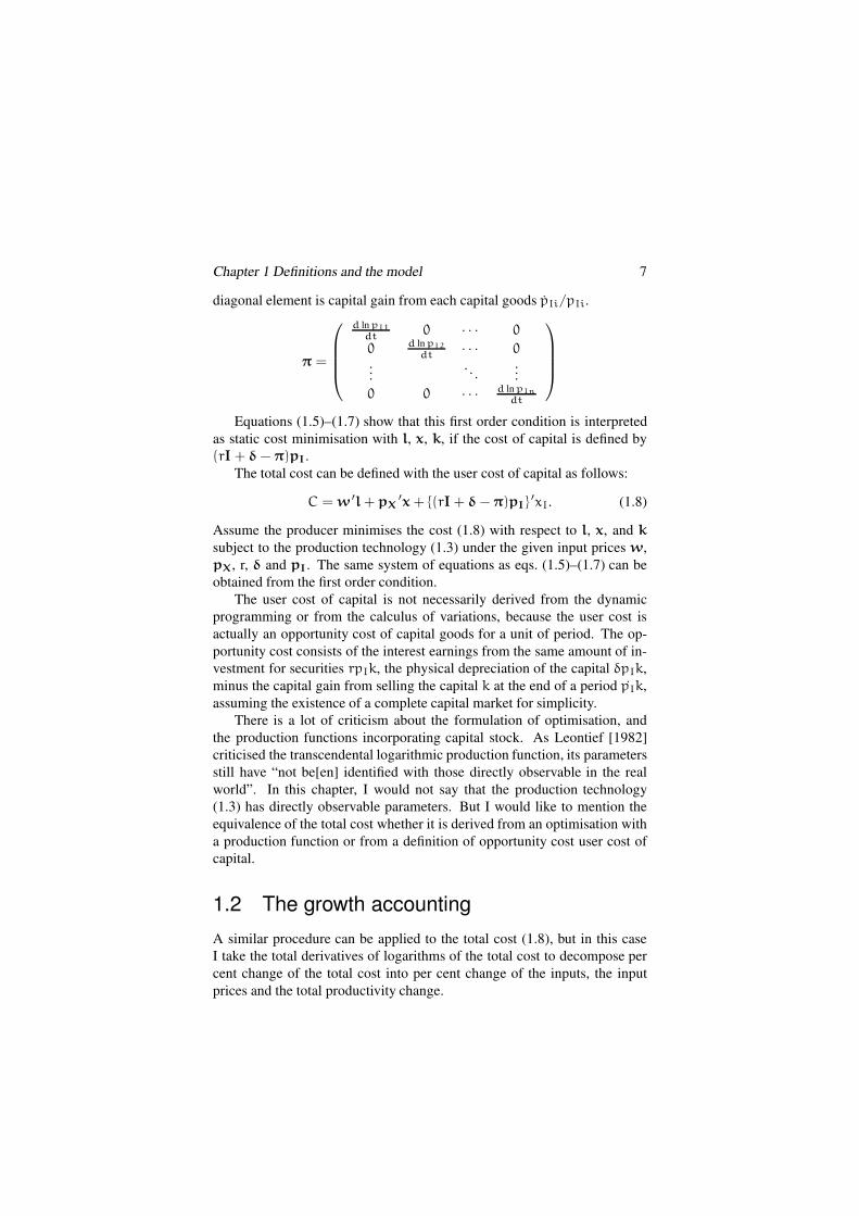
Chapter 1 Definitions and the model 7
diagonal element is capital gain from each capital goods pIi/pIi.
π =
d ln pI1
dt0 · · · 0
0 d ln pI2
dt· · · 0
.... . .
...
0 0 · · · d ln pIn
dt
Equations (1.5)–(1.7) show that this first order condition is interpreted
as static cost minimisation with l, x, k, if the cost of capital is defined by
(rI+ δ− π)pI.
The total cost can be defined with the user cost of capital as follows:
C = w ′l+ pX′x+ (rI+ δ− π)pI
′xI. (1.8)
Assume the producer minimises the cost (1.8) with respect to l, x, and k
subject to the production technology (1.3) under the given input prices w,
pX, r, δ and pI. The same system of equations as eqs. (1.5)–(1.7) can be
obtained from the first order condition.
The user cost of capital is not necessarily derived from the dynamic
programming or from the calculus of variations, because the user cost is
actually an opportunity cost of capital goods for a unit of period. The op-
portunity cost consists of the interest earnings from the same amount of in-
vestment for securities rpIk, the physical depreciation of the capital δpIk,
minus the capital gain from selling the capital k at the end of a period pIk,
assuming the existence of a complete capital market for simplicity.
There is a lot of criticism about the formulation of optimisation, and
the production functions incorporating capital stock. As Leontief [1982]
criticised the transcendental logarithmic production function, its parameters
still have “not be[en] identified with those directly observable in the real
world”. In this chapter, I would not say that the production technology
(1.3) has directly observable parameters. But I would like to mention the
equivalence of the total cost whether it is derived from an optimisation with
a production function or from a definition of opportunity cost user cost of
capital.
1.2 The growth accounting
A similar procedure can be applied to the total cost (1.8), but in this case
I take the total derivatives of logarithms of the total cost to decompose per
cent change of the total cost into per cent change of the inputs, the input
prices and the total productivity change.

8 Inter-industry propagation of techinical change
First take total derivative of logarithm of the total cost C:
d ln C = sL′ (d lnw+ d ln l) + sX
′ (d lnpX + d lnx)
+sK′ (d lnpK + d lnk) ,
(1.9)
where sL denotes the labour’s cost share vector of its element wili/C, sXdenotes the material’s cost share vector of its element pXixi/C, sK denotes
the capital’s cost share vector of its element pKiki/C, and pK denotes the
user cost of capital (rI+ δ− π)pI.
Next introduce the total factor productivity (TFP) that is the total output
per unit of the total inputs, and its growth rate is defined as follows:
d ln TFP = d ln X − (sL′d ln l+ sX
′d ln x+ sK′d lnk) , (1.10)
where d ln X denotes the total output index that is usually expressed in dif-
ferential form as
d ln X = sY′d lny.
sY denotes the value output share vector of its element piyi/∑
pjyj, and
y denotes the output vector as before.
Using the definition of the total factor productivity, equation (1.9) be-
comes as follows:
d ln C = sL′d lnw+ sX
′d lnpX + sK′d lnpK + d ln X − d ln TFP
d ln C/X = sL′d lnw+ sX
′d lnpX + sK′d lnpK − d ln TFP. (1.11)
This simply implies that the growth rate of the unit cost per unit of output
is equal to the sum of the growth rate of the wages, the material prices and
the user cost of capital, minus the growth rate of the total factor productivity.
The growth rate of the user cost of capital is expressed as the sum of
growth rate of its components. Since rI, δ, and π are all diagonal matrices,
d lnpK can be expressed using :

Chapter 1 Definitions and the model 9
d lnpK = d ln (rI+ δ− π)pI
= d ln
(r + δ1 − d ln pI1/dt)pI1
(r + δ2 − d ln pI2/dt)pI2
...
(r + δn − d ln pIn/dt)pIn
=
d ln (r + δ1 − d ln pI1/dt) + d ln pI1
d ln (r + δ2 − d ln pI2/dt) + d ln pI2
...
d ln (r + δn − d ln pIn/dt) + d ln pIn
=
d ln r+d ln δ1−d2 ln pI1/dt
r+δ1−d ln pI1/dt+ d ln pI1
d ln r+d ln δ2−d2 ln pI2/dt
r+δ2−d ln pI2/dt+ d ln pI2
...d ln r+d ln δn−d2 ln pIn/dt
r+δn−d ln pIn/dt+ d ln pIn
d lnpK = (rI+ δ− π)−1 (
(drI+ dδ)1− d2 lnpI/dt)
+ d lnpI,
(1.12)
where 1 denotes the column vector of one.
Before inserting (1.12) into (1.11), remember that the above formulation
is for a sector, which is to be considered as the j-th sector.
I will introduce the following assumptions for simplicity.
Assumption: No joint production The j-th sector produces the single
output Xj for all j. This means that Xj=y in the previous notation for y.
Assumption: Average cost Average cost of production Cj/Xj for the
j-th sector is equal to the output price of that sector pj.
Cj
Xj
= pj, (j = 1, . . ., n).
Assumption: Notation of the commodity Each output can be used as a
material and also as a capital goods, there is n kinds of commodities in the
economy. Prices for investment goods pI, for materials pX, and for outputs
p are no longer to be distinguished.
p = pI = pX

10 Inter-industry propagation of techinical change
Using these assumptions, the balance between input cost and output
price is written as follows:
d ln pj = sL′
jd lnw+ sX′
jd lnp
+sK′
j (rjI+ δj − π)−1 (
(drjI+ dδj)1 − d2 lnp/dt)
+sK′
jd lnp− d ln TFPj, (j = 1, . . ., n).
(1.13)
Divide both sides of the equation by dt, then the equation is expressed in
terms of the growth rate per unit of time.
d ln pj
dt= sL
′
jd lnw
dt+ sX
′
jd lnp
dt
+sK′
j (rjI+ δj − π)−1((
drj
dtI+
dδj
dt
)
1−d2 lnp
dt2
)
+sK′
jd lnp
dt−
d ln TFPj
dt, (j = 1, . . ., n).
(1.14)
Now we can introduce the balance equation of the whole economy.
1.3 Analytical framework
In this section, we derive the price equations of the whole economy in the
growth rate form. First of all, the notations are summerised as follows.
xij : input of the i-th good to produce the j-th good.
pi : price of the i-th good.
lj : labor input in the j–th sector.
wj : wage rate of lj
kij : stock of the i-th investment good used to produce the j-th good.
pKij : user cost of kij .
rj : interest rate of the j-th sector which produces the j-th good.
δij : depreciation rate of kij.
Cj : total factor cost of the j-th sector.
Xj : aggregated products of the j-th sector. Xjdef=
∑ni=1 xij.

Chapter 1 Definitions and the model 11
TFPj : total factor productivity of the j-th sector, defined by total input price
changes minus total output price changes, which is an equivalent defi-
nition to total output growth minus total input growth under the stable
profit rate.
SXij : cost share of the i-th input in the j-th sector.
SXijdef=
pixij
Cj
SKij : cost share of the i-th investment good in the j-th sector.
SKijdef=
pKijkij
Cj
SLj : labor’s cost share of the j-th sector.
SLjdef=
wjlj
Cj
Total cost of the j-th sector is as follows:
Cjdef=
n∑
i=1
pixij + wjlj +
n∑
i=1
pKijkij, (1.15)
where pKijdef= pi (rj + δij − d ln pi/dt).
In the growth rate form, total cost of the j-th sector is written as in the
next equation:
d ln Cj/Xj
dt
def=
n∑
i=1
SXij
d ln pi
dt+
n∑
i=1
SKij
d ln pKij
dt+SLj
d ln wj
dt−
d ln TFPj
dt.
(1.16)
Under perfect competition, we have, pj = Cj/Xj, and hece the price
equation becomes as follows:
d ln pj
dt=
n∑
i=1
SXij
d ln pi
dt+
n∑
i=1
SKij
d ln pKij
dt+ SLj
d ln wj
dt−
d ln TFPj
dt.
(1.17)
We find the term d ln pKij/dt (change in the cost of capital) in (1.17),
which needs more calculation to interpret. The change in the cost of capital

12 Inter-industry propagation of techinical change
can be broken down into the changes in interest rates, depreciation, and
capital gains or losses. Differenciating pKij gives:
d ln pKij
dt=
d ln pi
dt+
pirj
pKij
d ln rj
dt+
piδij
pKij
d ln δij
dt−
pi
pKij
d2 ln pi
dt2. (1.18)
If (1.18) is substituted into (1.17) for each sector, using the definiton of
pKij, we get:
∑ni=1 SKij
1rj+δij−dlnpi/dt
d2 ln pi
dt2 +∑n
i=1(∆ij − SXij − SKij)d ln pi
dt
= SLjd ln wj
dt+
∑ni=1 SKij
d ln pi
dt
(
drj
dt+
dδij
dt
)
−d ln TFPj
dt
(j = 1, . . . , n),
where ∆ij is a Kronecker’s delta, that is ∆ij = 0 when i = j, and
∆ii = 1 otherwise.
Equation (1.19) are the basic equations of our analysis in this book. pKij
is on the right hand side of (1.19) and hece (1.19) is not a reduced form
equation. Furthermore, cost–shares can vary in some or all of the prices.
If we assume that cost–shares are constant, it means that the underlying
production function is log-linear, i.e. Cobb–Douglas type.
1.4 The system in vector notation
For convenience, I would like to introduce vector notation for the system.
In the economy as a whole, the above system of equations is described as
follows:
d lnpdt
= SXd lnp
dt+ SK
d lnpdt
− Srd2 lnp
dt2
+SLd lnw
dt+(
RdtSr+ Sd
)
1− d lnTFPdt
.(1.19)
The growth account equations (1.19) corresponds to the Leontief’s price
equation (1.23), as we see later in this chapter.
Again, definitions of the matrices are as follows:
SL =
sL11 sL21 · · · sLnL1
sL12 sL22 · · · sLnL2
......
...
sL1n sL2n · · · sLnLn

Chapter 1 Definitions and the model 13
SX =
sX11 sX21 · · · sXn1
sX12 sX22 · · · sXn2
......
...
sX1n sX2n · · · sXnn
dR
dt=
dr1
dt0 · · · 0
0 dr2
dt· · · 0
.... . .
...
0 0 · · · drn
dt
Sr =
SK11
r1+δ11−d ln p1
dt
SK21
r1+δ21−d ln p2
dt
· · · SKn1
r1+δn1−d ln pn
dtSK12
r2+δ12−d ln p1
dt
SK22
r2+δ22−d ln p2
dt
· · · SKn2
r2+δn2−d ln pn
dt
......
...SK1n
rn+δ1n−d ln p1
dt
SK2n
rn+δ2n−d ln p2
dt
· · · SKnn
rn+δnn−d ln pn
dt
Sd =
SK11dδ11
dt
r1+δ11−d ln p1
dt
SK21dδ21
dt
r1+δ21−d ln p2
dt
· · · SKn1dδn1
dt
r1+δn1−d ln pn
dt
SK12dδ12
dt
r2+δ12−d ln p1
dt
SK22dδ22
dt
r2+δ22−d ln p2
dt
· · · SKn2dδn2
dt
r2+δn2−d ln pn
dt
......
...SK1n
dδ1ndt
rn+δ1n−d ln p1
dt
SK2ndδ2n
dt
rn+δ2n−d ln p2
dt
· · · SKnndδnn
dt
rn+δnn−d ln pn
dt
SK =
sK11 sK21 · · · sKn1
sK12 sK22 · · · sKn2
......
...
sK1n sK2n · · · sKnn
.
Definitions of the vectors are as follows:
d lnp
dt=
d ln p1
dtd ln p2
dt...
d ln pn
dt
d lnw
dt=
d ln w1
dtd ln w2
dt...
d ln wnL
dt

14 Inter-industry propagation of techinical change
d lnTFP
dt=
d ln TFP1
dtd ln TFP2
dt...
d ln TFPn
dt
d2 lnp
dt2=
d2 ln p1
dt2
d2 ln p2
dt2
...d2 ln pn
dt2
.
The other definitions of variables are as follows:
sLij =wilij
Cj
, sXij =pixij
Cj
SKij = sKij =pKikij
Cj
=pi
(
rj+δij−d ln pi
dt
)
kij
Cj.
sLij is the i-th labour’s cost share in the j-th sector, likewise sXij is the i-th
material’s cost share in the j-th sector, and sKij is the i-th capital goods’ cost
share in the j-th sector. There are nL types of labour, n types of materials
and capital goods.
After transposing the terms with d lnp/dt to the left hand side in (1.19),
the system becomes as follows:
Srd2 lnp
dt2 + (I− SX − SK)d lnp
dt= −d lnTFP
dt+ SL
d lnwdt
+(
dRdtSr+ Sd
)
1.(1.20)
I investigated this system of equations, which is non-linear with respect to
d lnp/dt, because Sr includes d lnp/dt, even if all the cost share matrices
are assumed to be constant.2 This system is homogeneous degree zero in
prices, because the equations do not change if all the prices grow at λ > 0,
λp, λw, when
(I− SX − SK − SL)1 = 0.
If wagesw are adjusted to cancel the effect of the total factor productiv-
ity fluctuation, while the interest rate and the depreciation keep unchanged,
the system becomes autonomous.
2Hayami[1993] proposed the same equations as a different form. Although my previous
formulation contains errors of notations, the two sector model in that paper is exactly the same
as this. As to nonlinear dynamical systems see for example, Guckenheimer Holms [1990].

Chapter 1 Definitions and the model 15
1.5 An implication to the Leontief’s dyanamic
inverse
Leontief dynamics [1970] is the system of equations that describes physical
balance of demand and supply.
xt −Atxt − Bt+1(xt+1 − xt) = ct, (1.21)
where At denotes the input coefficient matrix at t, and Bt+1 denotes the
capital coefficient matrix, “capital goods produced in year t are assumed to
be installed and put into operation in the next year t+1”, and ct denotes final
demand vector.3
Leontief [1970] proposes the following associated cost accounting, which
is dual to (1.21).
pt = A ′
tpt + (1 + rt−1)B ′
tpt−1 − B ′
t+1pt + vt, (1.22)
where rt−1 denotes the annual money rate of interest prevailing in that year,
and vt a vector of the value added per unit of its output. This equation can
be rewritten as follows:
pt = A ′
tpt + (rt−1I− π)B ′
tpt−1 − (B ′
t+1 − B ′
t)pt + vt, (1.23)
This system of equations implies that the price of output pt is equal to
the sum of the unit cost of materials A ′
tpt, the value added per output vt,
which includes employment cost and depreciation, and the user cost of net
capital (rt−1I−π)B ′
tpt−1, minus the technical change (B ′
t+1−B ′
t)pt. The
dynamic inverse price equation is precisely analogous to our price equation
(1.8) except that it ignores the depreciation. If we take further time diffrence
of (1.23), we can obtain the descrete approximaiton of our system.
3Leontief [1970], and reprinted in Leontief [1986] p.295.


Chapter 2
Non-stochastic models
In this chapter, I would like to explore four examples of non-stochasitic
models. First of all, the simple one sector model is to be analysed. Next, I
derive two sector model that has the same property as the one sector model.
And third, I calculate the general two sector model with various parameter
values. The simulations will reveal the basic properties of this model. Fi-
nally, I investigate the autonomouse system of this model, which presents
the system’s property on the price propagation.
2.1 One-sector model
The price equation system (1.19) takes the simplest form in the one-sector
model.
SK
p
ρ
d2 ln p
dt2+ (1 − SX − SK)
d ln p
dt
= SL
d ln w
dt+ SK
1
pK
(
dr
dt+
dδ
dt
)
−d ln TFP
dt(2.1)
Next substituting pK = p(r + δ − d ln p/dt) into the above equation,
we obtain
17

18 Inter-industry propagation of techinical change
d2 ln p
dt2−
(1 − SX − SK)
SK
(
d ln p
dt
)2
+
(
1
SK
(
SL
d ln w
dt−
d ln TFP
dt
)
+ (r + δ)1 − (SX + SK)
SK
)
d ln p
dt
=
(
dr
dt+
dδ
dt
)
+(r + δ)
SK
(
SL
d ln w
dt−
d ln TFP
dt
)
. (2.2)
For analytical convenience, we introduce the following parameters and
variables.
a = (1 − SX − SK)/SK > 0
R(t) = r + δ > 0
R ′(t) = dr/dt + dδ/dt
s(t) = [SLd ln w/dt − d ln TFP/dt] /SK
y(t) = d ln p/dt
Then equation (2.2) becomes the following first order ordinary differen-
tial equation:
y ′(t) − ay(t)2 + [s(t) + aR(t)]y(t) = R ′(t) + R(t)s(t)
Equation (2.3) is a nonlinear differential equation of the Riccati type.
Thus it is not possible to solve it generally by the integration method (see
Yoshida [1977]).
In this section, we assume that R(t) and s(t) are constant over time.
We transform variable y(t) as follows: −a · y(t) = u ′(t)/u(t), where
u ′(t) = du(t)/dt. Then equation (2.3) becomes the following 2nd order
ordinary linear differential equation:
u ′′(t) + [s + a · R] u ′(t) + a · R · s · u(t) = 0. (2.3)
Equation (2.3) has two characteristic roots of real numbers, because its
determinant D is positive.
D = (s − aR)2 ≥ 0 (2.4)

Chapter 2 Non-stochastic models 19
And the solution of (2.3) is obtained by (2.5),
u(t) = 1s−a·R
([s · u(0) + u ′(0)] exp (−a · R · t)− [a · R · u(0) + u ′(0)] exp (−s · t)) (2.5)
where u(0) and u ′(0) are the initial conditions and p(t) = C1/a/u(t)1/a.
Because a · R > 0, the first term of the left hand side of (2.5) converges to
0, as time t goes to infinity. Whether the second term of the left hand side
of (2.5) converges or diverges depends on whether s is positive or negative.
Thhe initial condition [a · R · u(0) + u ′(0)] is positive in sign, because it is
reduced to r+δ−d ln p(0)/dt, which is positive in normal situations. If s is
negative, then u(t) becomes infinitely large, and p(t)(= p(0)[u(0)/u(t)]1/a )
converges to 0. On the other hand, if s is positive, u(t) and p(t) both con-
verge.
2.2 Simplified two-sector model
In a two sector model, the equation (1.19) can be written explicitly as fol-
lows:
SK11
(
r1 + δ21 − d ln p2
dt
)
d2 ln p1
dt2 + SK21
(
r1 + δ11 − d ln p1
dt
)
d2 ln p2
dt2
+(
r1 + δ11 − d ln p1
dt
)(
r1 + δ21 − d ln p2
dt
)
×(
(1 − (SX11 + SK11)) d ln p1
dt− (SX21 + SK21) d ln p2
dt
)
= SK11
(
r1 + δ21 − d ln p2
dt
)
(
dr1
dt+ dδ11
dt
)
+ SK21
(
r1 + δ11 − d ln p1
dt
)
(
dr2
dt+ dδ21
dt
)
+(
r1 + δ11 − d ln p1
dt
)(
r1 + δ21 − d ln p2
dt
)
(
SL1d ln w1
dt− d ln TFP1
dt
)
(2.6)
SK12
(
r2 + δ22 − d ln p1
dt
)
d2 ln p1
dt2 + SK22
(
r2 + δ12 − d ln p2
dt
)
d2 ln p2
dt2
+(
r2 + δ12 − d ln p1
dt
)(
r2 + δ22 − d ln p2
dt
)
×(
(1 − (SX22 + SK22)) d ln p2
dt− (SX12 + SK12) d ln p1
dt
)
= SK12
(
r2 + δ22 − d ln p2
dt
)
(
dr1
dt+ dδ11
dt
)
+ SK22
(
r2 + δ12 − d ln p1
dt
)
(
dr2
dt+ dδ22
dt
)
+(
r2 + δ12 − d ln p1
dt
)(
r2 + δ22 − d ln p2
dt
)
(
SL2d ln w2
dt− d ln TFP2
dt
)
(2.7)

20 Inter-industry propagation of techinical change
For simplification, it is assumed that the 2nd sector does not produce
investment goods, thus we set SK21, SK22 = 0. Equations (2.6) and (2.7)
become as follows:
SK11d2 ln p1
dt2 +(
r1 + δ11 − d ln p1
dt
)
(1 − (SX11 + SK11)) d ln p1
dt
= SK11
(
dr1
dt+ dδ11
dt
)
+(
r1 + δ11 − d ln p1
dt
)
(
SL1d ln w1
dt− d ln TFP1
dt
)
(2.8)
SK12d2 ln p1
dt2
−(
r2 + δ12 − d ln p1
dt
)(
(SX12 + SK12) d ln p1
dt− (1 − SX22) d ln p2
dt
)
= SK12
(
dr2
dt+ dδ12
dt
)
+(
r2 + δ12 − d ln p1
dt
)
(
SL2d ln w2
dt− d ln TFP2
dt
)
(2.9)
Solving (2.8) for d2 ln p1/dt2, and substituting this expersson into (2.9),
we obtain
SK11 (1 − Wa22)
(
r2 + δ12 −d ln p1
dt
)
d ln p2
dt
= (SK11SX12 + SK12 (1 − SX11))
(
d ln p1
dt
)2
+
[
SK11 (SX12 + SK12) (r2 + δ12)
+SK12 (r1 + δ11) (1 − (SX11 + SK11))
−SK11
(
SL2
d ln w2
dt−
d ln TFP2
dt
)
+SK12
(
SL1
d ln w1
dt−
d ln TFP1
dt
)
]
d ln p1
dt
+ SK11SK12
(
dr2
dt+
δ12
dt−
dr1
dt−
dr1
dt−
dδ11
dt
)
− SK12 (r1 + δ11)
(
SL1
d ln w1
dt−
d ln TFP1
dt
)
+ SK11 (r2 + δ12)
(
SL2
d ln w2
dt−
d ln TFP2
dt
)
. (2.10)
If we assume further the following restrictions, (2.10) will take a simpler
form as in the following (2.11).
Chapter 2 Non-stochastic models 21
SX = SX12 = SX11,
SK = SK11 = SK12,
R = r2 + δ12 = r1 + δ11,
d ln p2
dt=
1
1 − SX
(
d ln p1
dt− SL1
d ln w1
dt+ SL2
d ln w2
dt
+d ln TFP1
dt−
d ln TFP2
dt
)
(2.11)
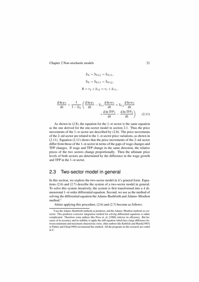
As shown in (2.8), the equation for the 1–st sector is the same equation
as the one derived for the one-sector model in section 2.1. Thus the price
movements of the 1–st sector are described by (2.8). The price movements
of the 2–nd sector are related to the 1–st sector price variations, as shown in
(2.11). Equation (2.11) shows that the price movements of the 2–nd sector
differ from those of the 1–st sector in terms of the gaps of wage changes and
TFP changes. If wage and TFP change in the same direction, the relative
prices of the two sectors change proportionally. Then the ultimate price
levels of both sectors are determined by the difference in the wage growth
and TFP in the 1–st sector.
2.3 Two-sector model in general
In this section, we explore the two-sector model in it’s general form. Equa-
tions (2.6) and (2.7) describe the system of a two-sector model in general.
To solve this system iteratively, the system is first transformed into a 4 di-
mensional 1–st order differential equation. Second, we use as the method of
solving the differential equation the Adams-Bashforth and Adams–Moulton
method.1
Afeter applying this procedure, (2.6) and (2.7) become as follows:
1I use the Adams–Bashforth methods as predictor, and the Adams–Moulton methods as cor-
rector. This predictor–corrector integration method for solving differential equations is rather
complicated. Therefore some authors like Press et. al. [1988] criticize its efficiency. But be-
cause of its accuracy and its stability to apply the stiff equation which has a large difference be-
tween minimum and maximum chracteristic roots, other authors like Kubıcek and Marek[1983]
or Parker and Chua[1989] recommend this method. All the programs in this research are coded
in C.

22 Inter-industry propagation of techinical change
(
d2 ln p1
dt2
d2 ln p2
dt2
)
= 1D
SK22
(
R12 − d ln p1
dt
)
− SK21
(
R11 − d ln p1
dt
)
−SK12
(
R22 − d ln p2
dt
)
SK11
(
R21 − d ln p2
dt
)
×
(
R11 − d ln p1
dt
)(
R21 − d ln p2
dt
)
×[
s1 − (1 − SX11 − SK11) d ln p1
dt+ (SX21 + SK21) d ln p2
dt
]
(
R12 − d ln p1
dt
)(
R22 − d ln p2
dt
)
×[
s2 − (1 − SX22 − SK22) d ln p2
dt+ (SX12 + SK12) d ln p1
dt
]
+
(
dr1
dtdr2
dt
)
+
SK11
(
R21 − d ln p2
dt
)
dδ11
dt
+SK21
(
R11 − d ln p1
dt
)
dδ21
dt
SK12
(
R22 − d ln p2
dt
)
dδ12
dt
+SK22
(
R12 − d ln p1
dt
)
dδ22
dt
.
(2.12)
where,
Ddef= SK11SK22
(
R12 −d ln p1
dt
)(
R22 −d ln p2
dt
)
−SK12SK21
(
R11 −d ln p1
dt
)(
R22 −d ln p2
dt
)
. (2.13)
Rijdef= rj + δij. (2.14)
s1def= SL1
d ln w1
dt−
d ln TFP1
dt. (2.15)
s2def= SL2
d ln w2
dt−
d ln TFP2
dt. (2.16)
As previously defined, D is a function of d ln p1/dt and d ln p2/dt.
Therefore, we can get the solutions only for non-singular D, and there is
an unresolved issue of whether D is always non-singular or not. Some ex-
amples for illustrative purposees are found in Figure 2.1–2.6. Figugre 2.6
shows initially the irregular movements of price variations. It seems that
values of the s1 and s2 play an important role in determining the feature of
output price changes.
In these numerical experiments, the parameters of SXij, SKij, SL1, SL2
are aggregated and roughly calculated from Input–Output Table 1985(es-
pecially capital formation matrix, Japan Ministry of Internatal Trade and

Chapter 2 Non-stochastic models 23
Industry). Sector 1 is assumed to produce manufacturing commodities, and
sector 2 is assumed to produce service and construction activities. Both sec-
tors depend on capital goods produced in both sectors. For our purpose to
illustrate the heuristic mechanism of cyclical price variations, these tenta-
tively chosen values suffice but further data elaboration might be required to
display realistic price fluctuations of the economic system. However, s1, s2
provide a reasonable range of values for simulations.
Figure 2.1 shows very normal pattern of price variations. But the inter-
active effects between the two industries shows the downward pressure of
price changes.
Figure 2.2 gives an example of a capital gain effect of the 2nd indus-
try because of the high inflation rate of the 1st commodity. Its effect on
decreasing costs lasts for about four years in this simulation.
Figure 2.3 is comparable to Figure 2.1. In Figure 2.3, relatively high
productivity growth in the 1st sector results in decreasing effects of the 2nd
commodity price. Its way of effectiveness is compounded with cyclical mo-
tions and trends.
Conversely in Figures 2.4–2.5, the 2nd sector’s productivity grows rapidly.
In these cases, basically the same results are obtained as in Figure 2.3.
Lastly Figure 2.6 shows extraordinarily high productivity growth in the
1st sector. In the case of s1 = −0.9, we can get the results as reported in
Figure 2.6, but for the range of values between s1 = −0.4 and s1 = −0.8,
our calculations overflow.
Detailed results about whether the calculations overflow or not are also
given. Those diagrams show the likelihood of instability of the system with
different parameters values for the cost shares. The two potential sources of
overflow are as follows. One possible source is dynamic instability which
depends on the characteristic roots of the determinant D. The other source
is the numerical approximation method used which may cause overflow if
the differential equation is a stiff equation in the sense that it has both large
and small characteristic roots. The former case displays a dynamic prop-
erty of productivity growth, and the latter case shows the difficulty when
we treat continuous time variables as discrete time. In our numerical ex-
periments, I first set dt as 1/100 year and then in the diverging cases I set
dt as 1/200, but the diverging properties did not improve. Therefore, for
reasonably small time units, our results show the instability of the effects
of productivity growth for the whole economic system incorporating capital
gains. But these characteristics are more fully investigated in the nect sec-
tion. 2In the divergent case, the sign of determinant D is negative and its
absolute value become relatively large( but less than 1 ).

24 Inter-industry propagation of techinical change
−0.03
−0.025
−0.02
−0.015
−0.01
−0.005
0
0.005
0.01
0 2 4 6 8 10
dlnP/dt
year
’Sector 1’’Sector 2’
List of parameters in Figure 1
a11 = 0.610 a12 = 0.190 a21 = 0.095 a22 = 0.128
b11 = 0.095 b12 = 0.172 b21 = 0.050 b22 = 0.240
r11 = 0.100 r12 = 0.140 r21 = 0.080 r22 = 0.100
w11 = 0.705 w12 = 0.362 w21 = 0.145 w22 = 0.368
s1 = −0.010 s2 = 0.010
Figure 2.1: The change rate of the prices

Chapter 2 Non-stochastic models 25
−0.04
−0.02
0
0.02
0.04
0.06
0.08
0.1
0 2 4 6 8 10
dlnP/dt
year
’Sector 1’’Sector 2’
List of parameters in Figure 2
a11 = 0.610 a12 = 0.190 a21 = 0.095 a22 = 0.128
b11 = 0.095 b12 = 0.172 b21 = 0.050 b22 = 0.240
r11 = 0.100 r12 = 0.140 r21 = 0.080 r22 = 0.100
w11 = 0.705 w12 = 0.362 w21 = 0.145 w22 = 0.368
s1 = 0.100 s2 = 0.010
Figure 2.2: The change rate of the prices

26 Inter-industry propagation of techinical change
−1
−0.9
−0.8
−0.7
−0.6
−0.5
−0.4
−0.3
−0.2
−0.1
0
0.1
0 2 4 6 8 10
dlnP/dt
year
’Sector 1’’Sector 2’
List of parameters in Figure 3
a11 = 0.610 a12 = 0.190 a21 = 0.095 a22 = 0.128
b11 = 0.095 b12 = 0.172 b21 = 0.050 b22 = 0.240
r11 = 0.100 r12 = 0.140 r21 = 0.080 r22 = 0.100
w11 = 0.705 w12 = 0.362 w21 = 0.145 w22 = 0.368
s1 = −0.200 s2 = 0.010
Figure 2.3: The change rate of the prices

Chapter 2 Non-stochastic models 27
−0.25
−0.2
−0.15
−0.1
−0.05
0
0.05
0.1
0 2 4 6 8 10
dlnP/dt
year
’Sector 1’’Sector 2’
List of parameters in Figure 4
a11 = 0.610 a12 = 0.190 a21 = 0.095 a22 = 0.128
b11 = 0.095 b12 = 0.172 b21 = 0.050 b22 = 0.240
r11 = 0.100 r12 = 0.140 r21 = 0.080 r22 = 0.100
w11 = 0.705 w12 = 0.362 w21 = 0.145 w22 = 0.368
s1 = −0.010 s2 = 0.100
Figure 2.4: The change rate of the prices
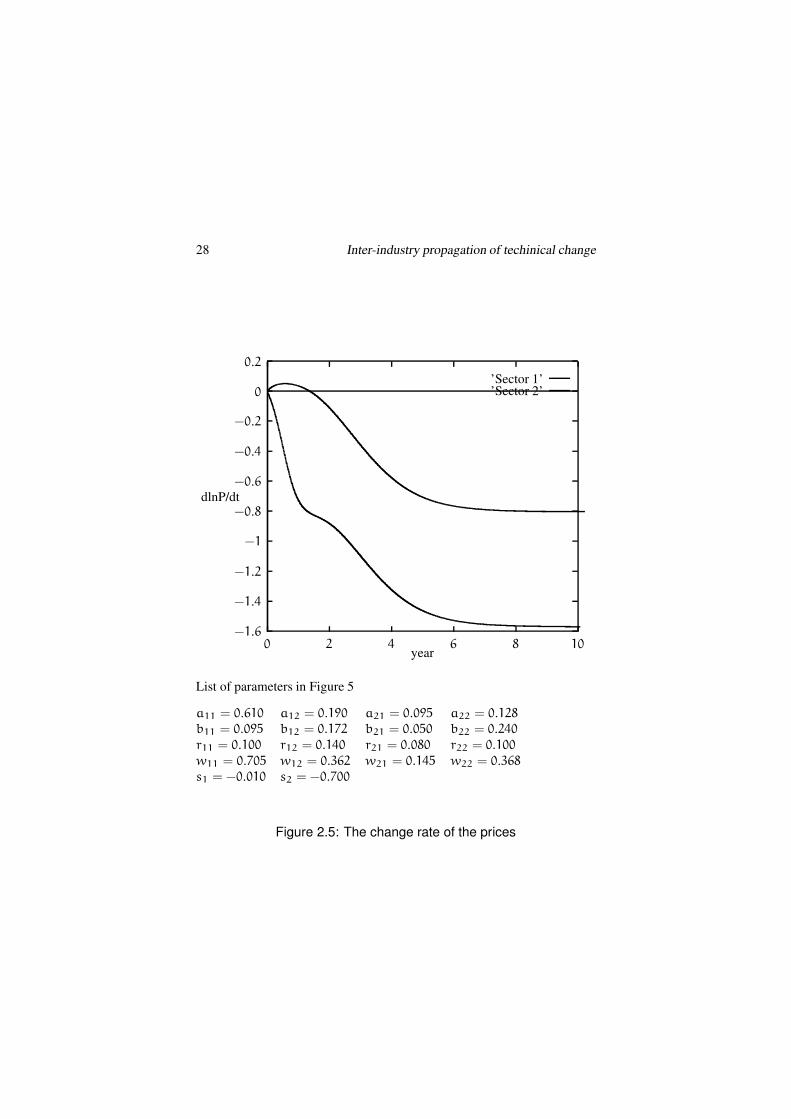
28 Inter-industry propagation of techinical change
−1.6
−1.4
−1.2
−1
−0.8
−0.6
−0.4
−0.2
0
0.2
0 2 4 6 8 10
dlnP/dt
year
’Sector 1’’Sector 2’
List of parameters in Figure 5
a11 = 0.610 a12 = 0.190 a21 = 0.095 a22 = 0.128
b11 = 0.095 b12 = 0.172 b21 = 0.050 b22 = 0.240
r11 = 0.100 r12 = 0.140 r21 = 0.080 r22 = 0.100
w11 = 0.705 w12 = 0.362 w21 = 0.145 w22 = 0.368
s1 = −0.010 s2 = −0.700
Figure 2.5: The change rate of the prices

Chapter 2 Non-stochastic models 29
−5
−4
−3
−2
−1
0
1
2
3
0 2 4 6 8 10
dlnP/dt
year
’Sector 1’’Sector 2’
List of parameters in Figure 6
a11 = 0.610 a12 = 0.190 a21 = 0.095 a22 = 0.128
b11 = 0.095 b12 = 0.172 b21 = 0.050 b22 = 0.240
r11 = 0.100 r12 = 0.140 r21 = 0.080 r22 = 0.100
w11 = 0.705 w12 = 0.362 w21 = 0.145 w22 = 0.368
s1 = −0.900 s2 = 0.010
Figure 2.6: The change rate of the prices

30 Inter-industry propagation of techinical change
2.4 An autonomous system of the price prop-
agation
In this section, an autonomous system of the price equation (2.17) is inves-
tigated. For simplicity, assume that all the cost shares are constant through
this section.
Assumption: Constant cost shares The cost shares SX, SK, SL are
constant over time.
Srd2 lnp
dt2 + (I− SX − SK)d lnp
dt= 0. (2.17)
This is, in fact, a first order differential equation system for the rate of price
changes. The system is non-linear, since Sr depends on d lnp/dt. Let z
denote d lnp/dt for simplicity, and the system is expressed as follows:
Sr(z)dzdt
= − (I− SX − SK) z,
d lnpdt
= z
(2.18)
There are two special cases to be highlighted. One of them is the singular
matrix Sr(z). If the matrix Sr(z) is singular, the system cannot describe
price changes. The other case is that the price change of a sector zi is equal
to rj + δij. In this latter case, one of the elements of the matrix Sr(z)
becomes infinitely positive or infinitely negative. The behaviour of the price
changes around these points may change drastically.
Except for these two cases, the system has a fixed point z = 0. And the
behaviour of the price changes around the fixed point can be described using
the eigenvalues of the following Jacobian matrix of first partial derivatives
at z = 0.
Jα(z) = −Dz
(
Sr(z)−1
(I− SX − SK) z)
, (2.19)
where Dz denotes a vector partial derivative operator [∂/∂zj] that operates
a vector valued function.
Jα with parameters α0 may have a zero eigenvalue at the fixed point
z = 0, the point (0, α0) should be a bifurcation point. But the following
discussion shows that this system does not have a bifurcation phenomenon.
The matrix Sr(z)−1
(I−SX−SK) can be expressed byW(z) in general.
Chapter 2 Non-stochastic models 31
W(z)z =
∑nj=1 W1j(z)zj∑nj=1 W2j(z)zj
...∑nj=1 Wnj(z)zj
Dz (W(z)z) = Dz
∑nj=1 W1j(z)zj∑nj=1 W2j(z)zj
...∑nj=1 Wnj(z)zj
Dz (W(z)z) =
∑nj=1
∂W1j
∂z1zj + W11
∑nj=1
∂W1j
∂z2zj + W12 . . .
∑nj=1
∂W2j
∂znzj + W1n
∑nj=1
∂W2j
∂z1zj + W21
∑nj=1
∂W2j
∂z2zj + W22 . . .
∑nj=1
∂W2j
∂znzj + W2n
...... . . .
...∑n
j=1∂Wnj
∂z1zj + Wn1
∑nj=1
∂Wnj
∂z2zj + Wn2 . . .
∑nj=1
∂Wnj
∂znzj + Wnn
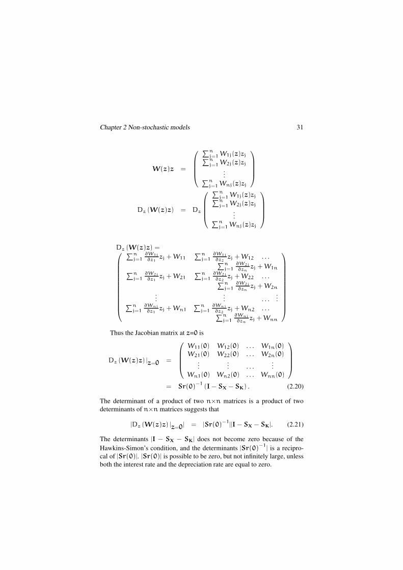
Thus the Jacobian matrix at z=0 is
Dz (W(z)z) |z=0 =
W11(0) W12(0) . . . W1n(0)
W21(0) W22(0) . . . W2n(0)...
... . . ....
Wn1(0) Wn2(0) . . . Wnn(0)
= Sr(0)−1
(I− SX − SK) . (2.20)
The determinant of a product of two n×n matrices is a product of two
determinants of n×n matrices suggests that
|Dz (W(z)z) |z=0| = |Sr(0)−1
||I− SX − SK|. (2.21)
The determinants |I − SX − SK| does not become zero because of the
Hawkins-Simon’s condition, and the determinants |Sr(0)−1
| is a recipro-
cal of |Sr(0)|. |Sr(0)| is possible to be zero, but not infinitely large, unless
both the interest rate and the depreciation rate are equal to zero.

32 Inter-industry propagation of techinical change
2.4.1 Two-sector autonomous model
To illustrate the eigenvalues of the Jacobian matrix Jα(z), I derived the two
sector system explicitly. The equation system can be described as follows:
(
z1
z2
)
= −
(
SK11
r1+δ11−z1
SK21
r1+δ21−z2SK12
r2+δ12−z1
SK22
r2+δ22−z2
)−1
×(
1 − SX11 − SK11 −SX21 − SK21
−SX12 − SK12 1 − SX22 − SK22
)(
z1
z2
)
,
(2.22)
or
(
z1
z2
)
= −1
D(z)
(
(1−SX11−SK11)SK22
r2+δ22−z2+
(SX12+SK12)SK21
r1+δ21−z2
)
z1
−(
(1−SX22−SK22)SK21
r1+δ21−z2+
(SX21+SK21)SK22
r2+δ22−z2
)
z2
−(
(1−SX11−SK11)SK12
r2+δ12−z1+
(SX12+SK12)SK11
r1+δ11−z1
)
z1
+(
(1−SX22−SK22)SK21
r1+δ11−z1+
(SX21+SK21)SK12
r2+δ12−z1
)
z2
,
(2.23)
where D is the determinant of Sr,
D(z) =SK11SK22
(r1 + δ11 − z1)(r2 + δ22 − z2)−
SK12SK21
(r1 + δ21 − z2)(r2 + δ12 − z1).
2.4.2 Behaviour around the fixed point z=0
Equation (2.23) is still complicated to calculate the Jacobian matrix, but
substituting z=0 into the Jacobian matrix makes all the derivatives related
with fractions disappear.
Jα(0) = 1
D(0)
−(
(1−SX11−SK11)SK22
r2+δ22+
(SX12+SK12)SK21
r1+δ21
)
(
(1−SX11−SK11)SK12
r2+δ12+
(SX12+SK12)SK11
r1+δ11
)
(
(1−SX22−SK22)SK21
r1+δ21+
(SX21+SK21)SK22
r2+δ22
)
−(
(1−SX22−SK22)SK11
r1+δ11+
(SX21+SK21)SK12
r2+δ12
)
.
(2.24)
D(0) is defined as
D(0) =SK11SK22
(r1 + δ11)(r2 + δ22)−
SK12SK21
(r1 + δ21)(r2 + δ12). (2.25)

Chapter 2 Non-stochastic models 33
The system has two real eigenvalues due to the fact that product of the
off diagonal elements of the Jacobian matrix Jα(0) is positive.3
It can be shown that the determinant of Jα(0) is
|Jα(0)| = 1
D(0)2
((1−SX11−SK11)SK22
r2+δ22+
(SX12+SK12)SK21
r1+δ21
)
×(
(1−SX22−SK22)SK11
r1+δ11+
(SX21+SK21)SK12
r2+δ12
)
−(
(1−SX22−SK22)SK21
r1+δ21+
(SX21+SK21)SK22
r2+δ22
)
×(
(1−SX11−SK11)SK12
r2+δ12+
(SX12+SK12)SK11
r1+δ11
)
= 1
D(0)|A|
where
|A| = (1 − SX11 − SK11)(1 − SX22 − SK22)
−(SX12 + SK12)(SX21 + SK21).(2.26)
Thus, the sign of the determinant |Jα(0)| depends on the sign of the
determinant D(0), while |A| is positive because of the Hawkins-Simon’s
condition4.
The following classification of the system can be obtained.
1. If |Jα(0)| > 0, i.e. D(0) > 0 the system has a fixed point of stable.
2. If |Jα(0)| < 0, i.e. D(0) < 0 the system has a fixed point of saddle.
3. The eigenvalues are diverge, when determinant D(0) is zero.
3The eigenvalues of a 2×2 matrixA can be derived as follows: λ denotes an eigenvalue of
A.
|λI −A| =
∣
∣
∣
∣
λ − a11 −a12−a21 λ − a22
∣
∣
∣
∣
= λ2 − (a11 + a22)λ+ a11a22 − a12a21 = 0.
The determinant D of the second order equation for λ is
D = (a11 + a22)2 − 4(a11a22 − a12a21)
= (a11 − a22)2 + 4a12a21.
Thus a12a21 < 0 is necessary for eigenvalues λ to have imaginary parts.4The Hawkins-Simon’s condition for a two sector input-output model is as follows, where
A is a input-coefficient matrix:
∣
∣
∣
∣
1− a11 −a12−a21 1 − a22
∣
∣
∣
∣
> 0.
The condition implies the system operates in positive production for all the sectors. In this
case, the inputs are not only material inputs SXij but also includes capital goods SKij . The
sum of both inputs needs to be in production possibility.

34 Inter-industry propagation of techinical change
D(0) > 0 can be rewrite from (2.25) as:
SK11SK22
SK12SK21
>(r1 + δ11)(r2 + δ22)
(r1 + δ21)(r2 + δ12).
The left hand side of the inequality means that relatively larger input coef-
ficients of their own capital goods than those of the other sector’s capital
goods, and the right hand side of the inequality shows that the price of their
own secotr’s capital goods is relatively smaller than the price of the other
sector’s capital goods. That is, given the relative cost, if the economic sys-
tem starts to rely more heavily on outsourced capital goods than before, the
system may hit a bifurcation point that shows saddle point instability. Sub-
stitute the definition of SKij into the condition, and it yields the condition in
terms of capital goods quantity:
k11
k21
>k12
k22
.
This again shows that the relatively large own capital input implies saddle
point instability of the system.5
The previous classification can be interpreted as follows.
1. IfSK11SK22
SK12SK21>
(r1+δ11)(r2+δ22)
(r1+δ21)(r2+δ12)or k11
k21> k12
k22, the system has a
stable fixed point.
2. IfSK11SK22
SK12SK21<
(r1+δ11)(r2+δ22)
(r1+δ21)(r2+δ12)or k11
k21< k12
k22, the system has a
fixed point of saddle.
3. IfSK11SK22
SK12SK21=
(r1+δ11)(r2+δ22)
(r1+δ21)(r2+δ12)or k11
k21= k12
k22, the eigenvalue of the
system is diverged.
2.4.3 Checking another fixed points z = 0
Set (2.23) equal to 0, there may be another fixed point in the system. Similar
discussions to the Jacobian matrix at z = 0, that the matrix Sr(z)−1(I −
SX − SK) must be singular to hold the equilibrium with z 6= 0. Because of
|I − SX − SK| > 0, it should be Sr(z)−1 = 0. This is impossible unless
Sr(z) is singular. I shall show next that there are many singular points.
5Benhabib and Nishimura [1998] assume single interest rate and single depreciation rate,
but introduce externality. They obtain indeterminacy, i.e. multiple equilibria in the two sector
model.

Chapter 2 Non-stochastic models 35
Nonetheless it is necessary to solve the equilibrium equations to show
the phase portraits of the systems. Solve the next equations for z1 and z2:
z1 = 0
z2 = 0(2.27)
That is(
(1−S11−SK11)SK22
r2+δ22−z2+
(S12+SK12)SK21
r1+δ21−z2
)
z1
−(
(1−S22−SK22)SK21
r1+δ21−z2+
(S21+SK21)SK22
r2+δ22−z2
)
z2 = 0
−(
(1−S11−SK11)SK12
r2+δ12−z1+
(S12+SK12)SK11
r1+δ11−z1
)
z1
+(
(1−S22−SK22)SK11
r1+δ11−z1+
(S21+SK21)SK12
r2+δ12−z1
)
z2 = 0
(2.28)
There are two asymptotes in each equation. One of these is a vertical or
horizontal line.
z2 =(1−S11−SK11)SK22(r1+δ21)+(S12+SK12)SK21(r2+δ22)
(1−S11−SK11)SK22+(S12+SK12)SK21,
for dz1
dt= 0 .
z1 =(1−S22−SK22)SK11(r2+δ12)+(S21+SK21)SK12(r1+δ11)
(1−S22−SK22)SK11+(S21+SK21)SK12,
for dz2
dt= 0
The other is a straight line of which the gradient does not depend on the
interest rate or the depreciation rate. However the line is too complicated to
describe in terms of the original parameters in the system Sij or SKij. It can
be shown that equation (2.28) can be arranged into the following form:
z1 = b1
d1z2 − a1d1−b1c1
d12 +
(a1d1−b1c1)c1
d12(c1−d1z2)
: for dz1
dt= 0
z2 = b2
d2z2 − a2d2−b2c2
d22 +
(a2d2−b2c2)c2
d22(c2−d2z2)
: for dz2
dt= 0,
where we temporally introduce the parameters ai, bi, ci, di (i = 1, 2).
a1 = (S21 + SK21)SK22(r1 + δ21)
+(1 − S22 − SK22)SK21(r2 + δ22)
b1 = (S21 + SK21)SK22 + (1 − S22 − SK22)SK21
c1 = (S12 + SK12)SK21(r2 + δ22)
+(1 − S11 − SK11)SK22(r1 + δ21)
d1 = (S12 + SK12)SK21 + (1 − S11 − SK11)SK22
a2 = (S12 + SK12)SK11(r2 + δ12)
+(1 − S11 − SK11)SK12(r1 + δ11)
b2 = (S12 + SK12)SK11 + (1 − S11 − SK11)SK12
c2 = (S21 + SK21)SK12(r1 + δ11)
+(1 − S22 − SK22)SK11(r2 + δ12)
d2 = (S21 + SK21)SK12 + (1 − S22 − SK22)SK11.

36 Inter-industry propagation of techinical change
If aidi − bici = 0, the second type of asymptotes disappears. Equation
dzi/dt = 0 becomes a straight line through the origin, and its gradient
does not depend on the interest rate or the depreciation rate. The gradient
is determined by the constants (here I assume that they are technological
factors) Sij, and SKij. Thus, the determinants aidi − bici = 0 are other
important factors in the system, and it can be shown as:
a1d1 − b1c1 = (r2 − r1 + δ22 − δ21)SK21SK22|A|
a2d2 − b2c2 = (r1 − r2 + δ11 − δ12)SK11SK12|A|,
where|A| = (1 − S11 − SK11)(1 − S22 − SK22)
−(S12 + SK12)(S21 + SK21).
The sign of |A| is again positive because of the Hawkins-Simon’s con-
dition in terms of the cost share, and each SKij is positive. The sign of
aidi − bici = 0 is determined by the magnitude of the interest rate and the
depreciation rate.
2.4.4 Classification of the autonomous system
Summary of the above discussions provides the general classification of the
two sector system. First, the system is stable at the fixed point, or saddle
at the fixed point. Second, the sign of intercept of the asymptote for each
equation z1 = 0 and z2 = 0, there are four cases. The other factor that is
not considered here is the magnitude of gradient of the asymptote.
There are at most four set of solutions for z1 and z2 including 0.The
other solutions are from the 3rd order polynomial equation, and the deter-
minant vanishes at the points. This situation can be occurred at the points,
where three curves intersect in Figures 2.4.4–2.4.4.
Case I The system is stable at the fixed point z = 0. The two asymptotes
for z1 = 0 and z2 = 0 both have positive intercepts to the other axis:
a1d1 −b1c1 > 0, a2d2 −b2c2 > 0. An economic meaning of these
conditions is that the nominal cost (interest rate and depreciation) of
capital goods is higher in the own sector’s investment that the other
sector’s.
Case II The system is stable at the fixed point z = 0. The two asymptotes
for z1 = 0 and z2 = 0 both have negative intercepts to the other axis:
a1d1 − b1c1 < 0, a2d2 − b2c2 < 0. The nominal cost (interest
rate and depreciation) of capital goods is lower in the own sector’s
investment that the other sector’s.
Chapter 2 Non-stochastic models 37
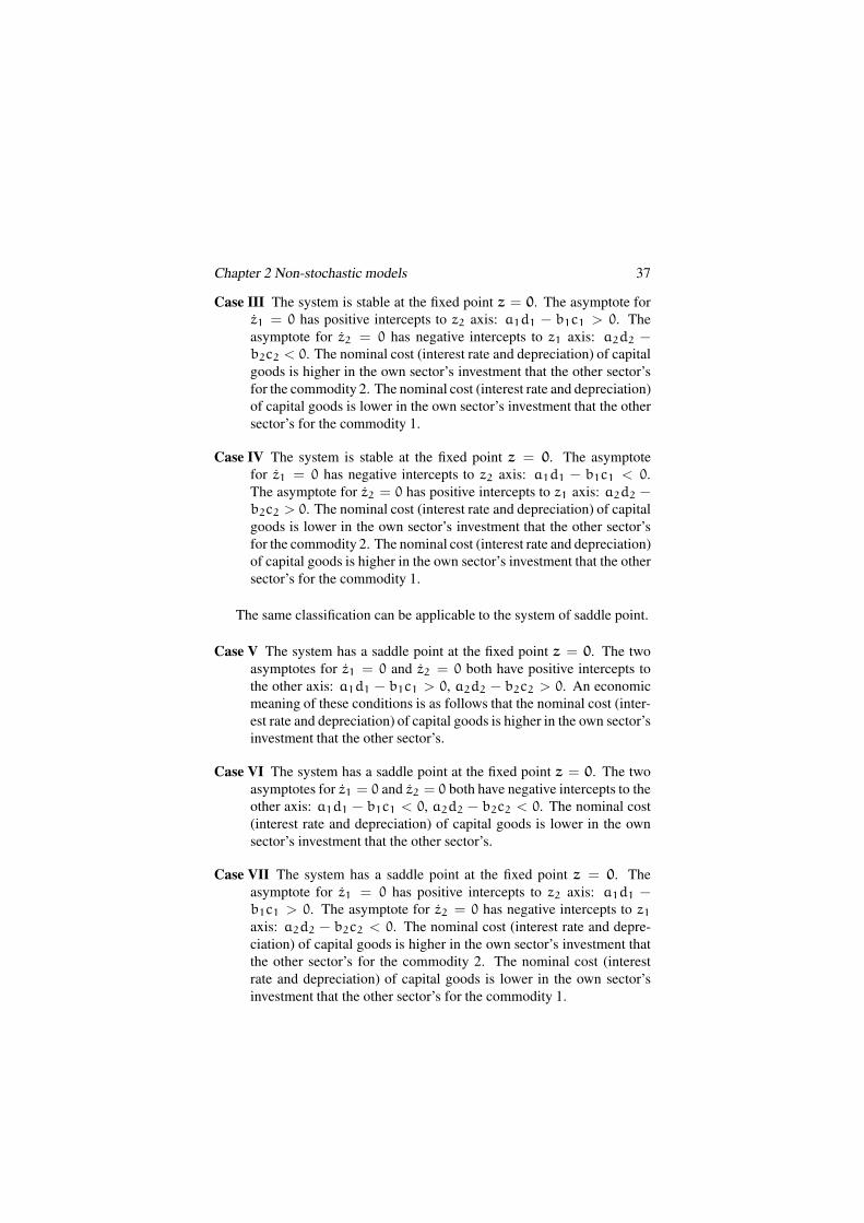
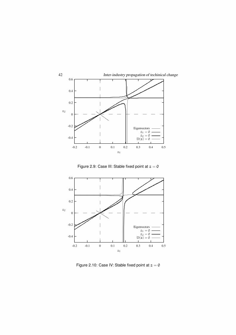
Case III The system is stable at the fixed point z = 0. The asymptote for
z1 = 0 has positive intercepts to z2 axis: a1d1 − b1c1 > 0. The
asymptote for z2 = 0 has negative intercepts to z1 axis: a2d2 −
b2c2 < 0. The nominal cost (interest rate and depreciation) of capital
goods is higher in the own sector’s investment that the other sector’s
for the commodity 2. The nominal cost (interest rate and depreciation)
of capital goods is lower in the own sector’s investment that the other
sector’s for the commodity 1.
Case IV The system is stable at the fixed point z = 0. The asymptote
for z1 = 0 has negative intercepts to z2 axis: a1d1 − b1c1 < 0.
The asymptote for z2 = 0 has positive intercepts to z1 axis: a2d2 −
b2c2 > 0. The nominal cost (interest rate and depreciation) of capital
goods is lower in the own sector’s investment that the other sector’s
for the commodity 2. The nominal cost (interest rate and depreciation)
of capital goods is higher in the own sector’s investment that the other
sector’s for the commodity 1.
The same classification can be applicable to the system of saddle point.
Case V The system has a saddle point at the fixed point z = 0. The two
asymptotes for z1 = 0 and z2 = 0 both have positive intercepts to
the other axis: a1d1 − b1c1 > 0, a2d2 − b2c2 > 0. An economic
meaning of these conditions is as follows that the nominal cost (inter-
est rate and depreciation) of capital goods is higher in the own sector’s
investment that the other sector’s.
Case VI The system has a saddle point at the fixed point z = 0. The two
asymptotes for z1 = 0 and z2 = 0 both have negative intercepts to the
other axis: a1d1 − b1c1 < 0, a2d2 − b2c2 < 0. The nominal cost
(interest rate and depreciation) of capital goods is lower in the own
sector’s investment that the other sector’s.
Case VII The system has a saddle point at the fixed point z = 0. The
asymptote for z1 = 0 has positive intercepts to z2 axis: a1d1 −
b1c1 > 0. The asymptote for z2 = 0 has negative intercepts to z1
axis: a2d2 − b2c2 < 0. The nominal cost (interest rate and depre-
ciation) of capital goods is higher in the own sector’s investment that
the other sector’s for the commodity 2. The nominal cost (interest
rate and depreciation) of capital goods is lower in the own sector’s
investment that the other sector’s for the commodity 1.

38 Inter-industry propagation of techinical change
Case VIII The system has a saddle point at the fixed point z = 0. The
asymptote for z1 = 0 has negative intercepts to z2 axis: a1d1 −
b1c1 < 0. The asymptote for z2 = 0 has positive intercepts to z1
axis: a2d2 − b2c2 > 0. The nominal cost (interest rate and depreci-
ation) of capital goods is lower in their own sector’s investment that
the other sector’s for the commodity 2. The nominal cost (interest
rate and depreciation) of capital goods is higher in their own sector’s
investment than the other sector’s for the commodity 1.
Parameter sets for the numerical illustration can be shown in Tables 2.1–
2.2.Note of Table 2.1:
This table shows that the system has a stable fixed point at z = 0
The difference between cases I–IV comes from the interest rate and the depreciation rate.The technological parameters are common for all cases.
a1d1 − b1c1 = (r2 − r1 + δ22 − δ21)SK21SK22|A|
a2d2 − b2c2 = (r1 − r2 + δ11 − δ12)SK11SK12|A|
a1d1 − b1c1 implies the difference of nominal cost of capital goods 2 between the ownsector 2 and the sector 1.
a2d2 − b2c2 implies the difference of nominal cost of capital goods 1 between the ownsector 1 and the sector 2.
|Jα(0)| denotes the Jacobian at the fixed point z = 0: positive means stable around thefixed point.
‘Eigenvalues’ are of the solution λ for the equation, |λI − Jα(0)| = 0.
‘Eigenvectors’ are the associate vectors z∗ with each eigenvalue, Jα(0)z∗ = λz∗.
Note of Table 2.2:
This table shows that the system has a saddle point at z = 0
The difference between cases I–IV and cases V–VIII comes from the technological pa-rameters, especially from SK.
Cases V–VIII shows larger capital goods input from the other sectors than own sectors.
Out sourcing of capital goods implies saddle point instability, as I explained in the text.The difference between cases I–IV comes from the interest rate and the depreciation rate.The technological parameters are common for all cases.
a1d1 − b1c1 = (r2 − r1 + δ22 − δ21)SK21SK22|A|
a2d2 − b2c2 = (r1 − r2 + δ11 − δ12)SK11SK12|A|
a1d1 − b1c1 implies the difference of nominal cost of capital goods 2 between the ownsector 2 and the sector 1.
a2d2 − b2c2 implies the difference of nominal cost of capital goods 1 between the ownsector 1 and the sector 2.
|Jα(0)| denotes the Jacobian at the fixed point z = 0: positive means stable around thefixed point.
‘Eigenvalues’ are of the solution λ for the equation, |λI − Jα(0)| = 0.
‘Eigenvectors’ are the associate vectors z∗ with each eigenvalue, Jα(0)z∗ = λz∗.

Ch
apter
2N
on
-stoch
asticm
od
els3
9Table 2.1: Parameter sets for the stable fixed point at z = 0
Case I Case II Case III Case IV
a1d1 − b1c1 > 0 a1d1 − b1c1 < 0 a1d1 − b1c1 > 0 a1d1 − b1c1 < 0
a2d2 − b2c2 > 0 a2d2 − b2c2 < 0 a2d2 − b2c2 < 0 a2d2 − b2c2 > 0
SX11 0.04 0.04 0.04 0.04
SX12 0.29 0.29 0.29 0.29
SX21 0.19 0.19 0.19 0.19
SX22 0.20 0.20 0.20 0.20
SK11 0.42 0.42 0.42 0.42
SK12 0.12 0.12 0.12 0.12
SK21 0.15 0.15 0.15 0.15
SK22 0.40 0.40 0.40 0.40
r1 0.05 0.05 0.03 0.06
r2 0.05 0.05 0.06 0.03
δ11 0.25 0.15 0.15 0.15
δ12 0.15 0.25 0.15 0.15
δ21 0.15 0.25 0.25 0.25
δ22 0.25 0.15 0.25 0.25
|Jα(0)| 0.0540706 0.01915 0.0283218 0.0302222
Eigenvalue −1.22028 −0.529053 −0.71621 −0.747259
Eigenvector
at z = 0
(
−0.731968
0.681339
) (
−0.726971
0.686668
) (
−0.538918
0.842358
) (
−0.59224
0.805762
)
Eigenvalue −0.0443101 −0.0361967 −0.039544 −0.0404441
Eigenvector
at z = 0
(
−0.615461
−0.788167
) (
−0.610981
−0.791646
) (
0.627869
0.778319
) (
0.61659
0.787285
)

40
Inter-in
du
stryp
rop
agatio
no
ftech
inical
chan
ge
Table 2.2: Parameter sets for the saddle point at z = 0
Case V Case VI Case VII Case VIII
a1d1 − b1c1 > 0 a1d1 − b1c1 < 0 a1d1 − b1c1 > 0 a1d1 − b1c1 < 0
a2d2 − b2c2 > 0 a2d2 − b2c2 < 0 a2d2 − b2c2 < 0 a2d2 − b2c2 > 0
SX11 0.04 0.04 0.04 0.04
SX12 0.29 0.29 0.29 0.29
SX21 0.19 0.19 0.19 0.19
SX22 0.20 0.20 0.20 0.20
SK11 0.14 0.14 0.14 0.14
SK12 0.32 0.32 0.32 0.32
SK21 0.15 0.15 0.15 0.15
SK22 0.10 0.10 0.10 0.10
r1 0.05 0.05 0.03 0.06
r2 0.05 0.05 0.06 0.03
δ11 0.25 0.15 0.15 0.15
δ12 0.15 0.25 0.15 0.15
δ21 0.15 0.25 0.25 0.25
δ22 0.25 0.15 0.25 0.25
|Jα(0)| −0.351 −1.99964 −0.648356 −0.589276
Eigenvalue 1.73559 8.77869 3.13194 2.87207
Eigenvector
at z = 0
(
0.508159
−0.861263
) (
0.502609
−0.864514
) (
0.380055
−0.924964
) (
0.358354
−0.933586
)
Eigenvalue −0.202237 −0.227783 −0.207014 −0.205174
Eigenvector
at z = 0
(
−0.560947
−0.827852
) (
−0.566327
−0.824181
) (
−0.564695
−0.8253
) (
−0.540816
−0.841141
)

Chapter 2 Non-stochastic models 41
Eigenvectors
z1 = 0z2 = 0
D(z) = 0-0.4
-0.2
0
0.2
0.4
0.6
-0.2 -0.1 0 0.1 0.2 0.3 0.4 0.5
z2
z1
Figure 2.7: Case I: Stable fixed point at z = 0
s
Eigenvectors
z1 = 0z2 = 0
D(z) = 0-0.4
-0.2
0
0.2
0.4
0.6
-0.2 -0.1 0 0.1 0.2 0.3 0.4 0.5
z2
z1
Figure 2.8: Case II: Stable fixed point at z = 0
42 Inter-industry propagation of techinical change
Eigenvectors
z1 = 0z2 = 0
D(z) = 0-0.4
-0.2
0
0.2
0.4
0.6
-0.2 -0.1 0 0.1 0.2 0.3 0.4 0.5
z2
z1
Figure 2.9: Case III: Stable fixed point at z = 0
Eigenvectors
z1 = 0z2 = 0
D(z) = 0-0.4
-0.2
0
0.2
0.4
0.6
-0.2 -0.1 0 0.1 0.2 0.3 0.4 0.5
z2
z1
Figure 2.10: Case IV: Stable fixed point at z = 0

Chapter 2 Non-stochastic models 43
Eigenvectors
z1 = 0z2 = 0
D(z) = 0-0.4
-0.2
0
0.2
0.4
0.6
-0.2 -0.1 0 0.1 0.2 0.3 0.4 0.5
z2
z1
Figure 2.11: Case V: Saddle point at z = 0
Eigenvectors
z1 = 0z2 = 0
D(z) = 0-0.4
-0.2
0
0.2
0.4
0.6
-0.2 -0.1 0 0.1 0.2 0.3 0.4 0.5
z2
z1
Figure 2.12: Case VI: Saddle point at z = 0

44 Inter-industry propagation of techinical change
Eigenvectors
z1 = 0z2 = 0
D(z) = 0-0.4
-0.2
0
0.2
0.4
0.6
-0.2 -0.1 0 0.1 0.2 0.3 0.4 0.5
z2
z1
Figure 2.13: Case VII: Saddle point at z = 0
Eigenvectors
z1 = 0z2 = 0
D(z) = 0-0.4
-0.2
0
0.2
0.4
0.6
-0.2 -0.1 0 0.1 0.2 0.3 0.4 0.5
z2
z1
Figure 2.14: Case VIII: Saddle point at z = 0

Chapter 3
The stochastic system and
its solutoin method
3.1 Random factor: an introdcution
This section surveys breafly how to introduce random factor into a system.
I would like to present its conditions and to give a perspective for the gen-
eralisation. There are many introductory explanations by mathematitian,
which reveal strict mathematical conditons. However, we cannot under-
stand how economic variables and data phenomenologically relate with the
conditions through the strict mathematical explanation.1.I am indebted to
Reichl [1980] and van Kampen [1992] greatly, and fundamentally to the
classical paper by Wang and Uhlenbeck [1945]. Here I would like to focus
on fluctuations of the economic varialbes.
For example, I assume that the rate of change of the total factor pro-
ductivity (TFP) obeys a stocastic process. The rate of change of TFP is a
random process, which is accelerated or decelerated by number of sucesses
and failures of technical progress. This is often assumed, but in fact it is
only a working hypothesis. Nevertheless, considering that each improve-
ment of technology is a very small step, but eventually these steps can be
aggregated into an increase of TFP, hece we can apply the central limit the-
orem to the movement of TFP. That means that the distribution of the rate
of change of TFP is assumed to be gaussian. In economics, mechanism of
technical change is given in general, and normally treated as a black box.
1Among the explanations by mathematitioans, L. C. G. Rogers [1997] is an excelent
overview of stochasitc processes in finance and easy to understand.
45

46 Inter-industry propagation of techinical change
Economics does not analyse whether the current prevailing technology is
superior or inferior to the past technologies, because it survives under the
economic competition.
Such a formulation is quite common in biology. It is assumed that the
gene frequency fluctuates under a stochastic process, when the biologist in-
troduce a stochastic process into an evolution. A gene of some phenotype
is assumed to be a mutually exclusive envent to a gene of the opposite phe-
notype. The model further assumes random mutation, and environmental
facors (parameters) that affect one of the phenotypes profitable.2 In this
formulation, gene itself is not affected by natural selection, but the pheno-
type. Past environmental history determines the present phenotype, but we
cannot know whether it is an evolution or not. Furthermore, even if there
were the same environmental history as the past again, there is no reason
that the same phenotype can survive. The model is a black box other than
gene frequency. We cannot formulate multiple phenotypes as in the biolog-
ical model, but we assumes that the level of TFP represents an adaptation
to economic environment at each time and that it is enough to describe the
survival of the fittest under the economic competition.
I would like to introduce such an economic stochastic process rather
formally in this section. Let X is a stochastic variable, a stochastic process
YX(t) = f(X, t) at time t, and the probability with the value YX(t) = y
is described by the probability density function of X, PX(x), and Dirac’s δ
function as follows:
P1(y, t) =
∫
δ(y − Yx(t))PX(x)dx, or
= < δ(y − Yx(t)) >, (3.1)
where Yx(t) = f(x, t) is a sample function of the stochastic process. If
YX(t) has values y1, y2, . . ., yn at n points t1, t2, . . ., tn, then its joint
density hierarchy function becomes as follows:
Pn((y1, t1), (y2, t2), . . . , (yn, tn))
=∫
δ(y1 − Yx(t1))δ(y2 − Yx(t2))· · ·δ(yn − Yx(tn))PX(x)dx
If a joint probability density hierarchy function Pn is satisfied with the fol-
lowing four conditions, and the mean exists, Pn can construct the stochastic
process completely. This is the Kolmogorov existence theorem, and the
proof is given by Billingsley [1995], for example.
1. Pn≥0
2See for example Kimura [1964].

Chapter 3 The stochastic system and its solution method 47
2. Pn is the same value, even if (yi, ti) and (yj, tj) are exchanged.
3.∫
Pn((y1, t1), (y2, t2), . . . , (yn, tn))dyn
= Pn−1((y1, t1), (y2, t2), . . . , (yn−1, tn−1)) (3.2)
4.∫
P1(y, t)dy = 1
In order to analyse concrete problems, we must introduce further as-
sumptions, such as stationarity, Markov, or Gauss distribution. First I would
like to show the limitation of stationarity. And second, I will introduce
Markov and finally derive the Fokker-Planck equation.
3.1.1 Stationary process and its limitation
If a stochastic process is stationary, the probability density hierarchy func-
tion Pn remains unchanged as time passes to any τ.∫
Pn((y1, t1), (y2, t2), . . . , (yn, tn))
= Pn−1((y1, t1 + τ), (y2, t2 + τ), . . . , (yn, tn + τ))(3.3)
In a stationary process, applying the Wiener-Khinchin theorem, and the
power spectrum I(ω) can be obtained by Fourier transpose of its autocorre-
lation function. In a stationary process, autocorrelation function φ(t1, t2)
is expressed by a fuction of time difference τ = t2 − t1.
φ(t1, t2) = < (Y(t1)− < Y(t1) >)(Y(t2)− < Y(t2) >) >
= < (Y(0)− < Y(0) >)(Y(τ)− < Y(τ) >) >
φ(τ) = < (Y(0)− < Y(0) >)(Y(τ)− < Y(τ) >) > (3.4)
During 0 < t < T a sample function of a stochastic process is a normal
function of t and it can be applicable to Fourier transformation. ωn = 2πnT
denotes the frequency. If YX is real number, the Fourier coefficient an has
an restriction of a−n = a∗
n.
Yx(t) =
∞∑
n=−∞
aneiωnt
an =1
T
∫T
0
Yx(t)e−iωntdt

48 Inter-industry propagation of techinical change
Fourier coefficient an within a small range of frequency has a strength
|an|2, and its average is defined by the spectrum density or the power stpec-
trum. Here, the Wiener-Khinchin theorem shows that the power spectrum
I(ω) is expressed by autocorrelation function φ(t) as follows:
I(ω) =1
2π
∫∞
−∞
φ(t)e−iωtdt.
The coefficient 12π
is dual to the Fourier inverse transformation. According
to the Wiener-Khinchin theorem, any stationary process can be obserbed by
autocorrelation, and has the power spectrum. If the process has a specific
distribution, the power spectrum has a simple form and becomes easy to
analyse. For example, the power spectrum is constant over every frequency,
the random effect has a white spectrum or is called by white noise.
Though the stationary process can apply only limited cases, as I explan
next, there are some cases such as the Wiener process that has a stationary
increment, which can be analysed by transforming the original process.
The next example is not a stationary process. For the time t and its
interval from 0 to T , n points are chosen and labled sequentially.
0 = t0 < t1 < t2 < · · · < tn < T
As time passes, the productivity y (for example the labour productivity and
its training cost) is also fluctuating. As a rapid fluctuation (increases of
labour productivity) costs more, the firm minimises its squared sum over n
stages. Let y0 = 0,yn+1 = 0 for convenience. Increase of productivity
is a stochastic variable, and the increments yi+1 − yi are mutually inde-
pendent. We focus on the adjustment cost that is increased by rapid labour
productivity changes, and assume that unit cost from productivity fluctua-
tion per unit of time is constant over the training stages i.
y12
t1
+(y2 − y1)2
t2 − t1
+ · · · + (yn − yn−1)2
tn − tn−1
+yn
2
T − tn
.
The distribution of productivity fluctuations is defined as follows:
Pn((y1, t1), (y2, t2), . . . , (yn, tn))
=(
2πTα
)1/2 ∏n−1i=1
(
α2π(ti−ti−1)
)1/2
exp(
−α2
(yi−yi−1)2
(ti−ti−1)
)
(3.5)
This satisfies with the Kolmogorov’s four conditions. But this is not station-
ary because of the autocorrelation.
< Y(t1)Y(t2) >=1
α
t1(T − t2)
T
Therefore, we cannot construct the power spectrum.

Chapter 3 The stochastic system and its solution method 49
3.1.2 Transition probability and the Chapman-Kolmogorovequation
As the stationary model is very limited, we introduce the Markov property
into the probability density hierarchy function Pn. There are many models
with Markov process, but few are known as non-Markov process. Non-
Markov process is a process with memory, but the memory term can be
eliminated by “contraction” or “projection” and eventually converted into
Markov process (Suzuki [1994]). In Markov process, the next relations are
established.
P1|n−1((yn, tn)|(y1, t1), (y2, t2), · · ·, (yn−1, tn−1))
= P1|1(yn, tn|yn−1, tn−1)
≡ P(yn, tn|yn−1, tn−1)
(3.6)
P1|n−1 is a conditional probability density hierarchy function with n − 1
pairs of conditions, and P(yn, tn|yn−1, tn−1) is a transition probability
density.
In Markov process, the probability density hierarchy function can be
expressed by the transition probability and its initial value P1(y1, t1). For
example, at time t1 the point was at y1, at time t2 the point moved to y2,
and at time t3, the point moved to y3. In this case, the probability density
hierarchy is expressed by the conditional probability density, that is, the
multiple of the transition probability from y1 to y2, and the conditional
probability of y3 given y1 and y2 as a condition. In case of Markov process,
the latter probability is the transition probability of y3 given the condition
y2.
P3((y1, t1), (y2, t2), (y3, t3))
= P2((y1, t1), (y2, t2))P1|2(y3, t3|(y1, t1), (y2, t2))
= P(y3, t3|y2, t2)P(y2, t2|y1, t1)P1(y1, t1)
(3.7)
The second line is integrated by y2,
P2((y1, t1), (y3, t3)) = P1(y1, t1)
∫
P(y3, t3|y2, t2)P(y2, t2|y1, t1)dy2.
From the definition of the conditional probability, under the condition that
the point was y1 at time t1, the probability of y3 at time t3 is given as
follows:
P(y3, t3|y1, t1) =
∫
P(y3, t3|y2, t2)P(y2, t2|y1, t1)dy2 (3.8)

50 Inter-industry propagation of techinical change
This is the Chapman-Kolmogorov equation. In Markov process, all proba-
bility density hierarchy functions are determined by the transition probabil-
ity. If it satisifies with the next consistency condition, any Markov process
is determined by the Chapman-Kolmogorov equation.
P1(y2, t2) =
∫
P(y2, t2|y1, t1)P1(y1, t1)dy1 (3.9)
3.1.3 The master equation
In this section, taking Taylar expansion of the transition probability, we
will derive the master equation, which is the transition probability in dif-
ferential form with respect to time, i.e. the differential form of Chapman-
Kolmogorov equation.
The transition probability defined on partial defferential with respect to
time is
∂P(y2, t2|y1, t1)
∂t2
= limτ→0
P(y2, t2 + τ|y1, t1) − P(y2, t2|y1, t1)
τ.
(3.10)
We will take Taylar expansion of P(y2, t2 + τ|y1, t1) with respect to τ
for evaluation of the above definiton. At the same time, the integration of
probability over the range must be normalised to one. That is
∫
P(y2, t2|y1, t1))dy2 = 1. (3.11)
An expansion with the normalisation condition is expressed as follows:
P(y2, t+τ|y1, t) = P(y2, t|y1, t)+τWt(y2|y1)−τa0P(y2, t|y1, t)+o(τ),
(3.12)
where Wt(y2|y1) =P(y2,t+τ|y1,t)
τ,a0 is obtained by the normalisation
condition:
a0(y1) =
∫
Wt(y|y1)dy. (3.13)
And P(y2, t|y1, t) becomes Dirac’s delta function by definition.
P(y2, t|y1, t) = δ(y2 − y1),
where o(τ) is a term satisfied with limτ→0 o(τ)/τ = 0.

Chapter 3 The stochastic system and its solution method 51
Equation (3.12) is applied to the integrand P(y3, t3|y2, t2) of the Chapman-
Kolmogorov equation (3.8). That is t2 = t,t3 = t + τ etc., we obtain
P(y3, t3|y1, t1) =
∫
δ(y3 − y2)(1 − τa0)P(y2, t2|y1, t1)dy2
+τ
∫
Wt2(y3|y2)P(y2, t2|y1, t1)dy2
P(y3, t2 + τ|y1, t1) = P(y3, t2|y1, t1)
+τ
∫
Wt2(y3|y2)P(y2, t2|y1, t1)dy2
−τ
∫
Wt2(y|y3)P(y3, t2|y1, t1)dy.
As t2→t3, the last integral variable of the right hand side y is changed to
y2,
∂P(y3,t3|y1,t1)
∂t3=∫
Wt3(y3 |y2)P(y2, t3|y1, t1) − Wt3
(y2|y3)P(y3, t3|y1, t1)dy2 .
(3.14)
This is the master equation. Simply it can be written as
∂P(y, t)
∂t=
∫
(Wt(y|y ′)P(y ′, t) − Wt(y′|y)P(y, t)) dy ′. (3.15)
3.1.4 The Fokker-Planck equation
As the master equation is a conposite equation of differential and integral,
although the analysis of it is easier than of the Chapman-Kolmogorov equa-
tion, much easier equation is preferable. In order to analyse more conve-
niently, we assume taking the short time enough not to allow a jump of y,
but at the same time the equation keeps Markov property. This assumption
derives the Fokker-Planck equation, which is a differential equation.3
Now using ξ of y’s jump and inserting y ′ = y − ξ, the master equation
becomes as follows:
∂P(y, t)
∂t=
∫
(Wt(y|y − ξ)P(y − ξ, t) − Wt(y − ξ|y)P(y, t)) dξ.
Then we take Taylor expansion of Wt(y|y − ξ)P(y − ξ, t) at y = y − ξ
3Fokker [1913] used a specail form, Planck [1917] derived it from the master equation, and
Kolmogorov [1931] gave the mathematical foundation.

52 Inter-industry propagation of techinical change
and y ′ = y with respect to ξ.
Wt(y|y − ξ)P(y − ξ, t) = Wt(y − ξ|y) −∂
∂y ′(Wt(y − ξ|y)P(y, t))ξ
+∂2
∂y ′2(Wt(y − ξ|y)P(y, t)) ξ2 + o(ξ2).
After inserting this equation into the original master equation, and exchange
the differential operation under the integration, we obtain the following ex-
pansion:
∂P(y,t)
∂t= − ∂
∂y ′
(∫Wt(y − ξ|y)ξdξP(y, t)
)
+12
∂2
∂y ′2
(∫Wt(y − ξ|y)ξ2dξP(y, t)
)
+ . . . .
Here we assume that there exists δ > 0 satisfied with the next three condi-
tions.W(y|y ′)≈0, y ′ = y − ξ, |ξ| > δ
W(y|y ′ + ∆y)≈W(y|y ′), |∆y| < δ
P(y + ∆y, t)≈P(y, t), |∆y| < δ
Hence ignoring the higher order terms, the above expansion can be written
as follows:
∂P(y,t)
∂t= − ∂
∂y
(∫Wt(y − ξ|y)ξdξP(y, t)
)
+12
∂2
∂y2
(∫Wt(y − ξ|y)ξ2dξP(y, t)
)
.
The Fokker-Planck equation is obtained using the jump moment an, that is,
∂P(y,t)
∂t= − ∂
∂y(a1(y)P(y, t))
+12
∂2
∂y2 (a2(y)P(y, t)) ,(3.16)
where an(y) =
∫
ξnW(y − ξ|y)dξ.
If we take into account of all the higher terms of Taylor expansion, the
equaiton becomes the Kramers-Moyal expansion. The Fokker-Planck equa-
tion is obtained under the condition of infinitesimal jump, but it is easy to
analyse because it is a differential equation.4.
The stochastic differential equation in financial economics is also a part
of the examples of the Fokker-Planck equation. Therefore it requires the
4Section 3.2 shows solutions of some special cases, but only a few strict solustions have
ever known.

Chapter 3 The stochastic system and its solution method 53
same assumptions as the above. Non-Markov process can be approaximated
by projection as a Markov process. But the infinitesimal jump is very restric-
tive, in addtion to Ornstein-Uhenbeck process that is stationary, Markovian,
and Gaussian but does not include infinitesimal jump, the jump with a dis-
tribution of the quadratic funtion has been introduced.5
Here we assume that the total factor productivity obeys the stochastic
process with infinitesimal jump. This assumption leads to the idea that the
techinical progress is actually gradual. As we see the new technology that
transcends many conditions of the time has long been forgotten from the
society, a new technology may require some continuity to the previous when
it spreads as an technical progress in the economy.
The Fokker-Planck equation is linear with respect to P. When we call a
linear Fokker-Planck equation, we assume that a1(y) is a linear function of
y, and a2(y) is constant. Conveniently, the Fokker-Planck equation can be
determined and solvable, when the jump moments up to the second order,
a1(y)(the drift term) and a2(y)(the diffusion term) are observable. Further-
more, these values are independent from time, you do not need to know all
the history of the moments. In addition to such merits, the Fokker-Planck
equation is related to the Langevin equation, which is easy to introduce ran-
dom factors. However, there is a subtle problem in interpretation of the
Langevin equation. In the linear case, there is no discrepancy between the
data from macroscopic observation and the Fokker-Planck equation, but in
the non-linear case, you cannot ignore effects from the diffusion coefficient
a2(y), and it becomes difficult to identify a1(y). In such a case, the Ω ex-
pasion method for the master equation should be apllied.6 If the equilibrium
is unstable, the Ω expansion method for the master equation is not useful,
then you should apply the scaling theory on order formation.7.
3.1.5 The Langevin equation
We explain the Langevin equation that treats a random factor and that is
widely used in physics. If the random factor distributes with Gaussian dis-
tribution, the Langevin equation is identical to the Fokker-Planck equaiton.
Ito’s stochastic differential equation are extremely often used in economics,
but the random factor (diffution parameter) in the Langevin equation can
be equally applicable with both Itp’s interpretaion and Stratonovich’s. But
the different interpretation leads to the different Fokker-Planck equation.
5Babbs and Webber[1997] and El-Jahel et al.[1997] demonstrate that the distribution of an
asset price fluctuation become leptokurtic without the infinitesimal jump.6Ω is typically a parameter of the size of system.7van Kampen[1992], p. 96,Suzuki[1994], p. 243.

54 Inter-industry propagation of techinical change
Interpretation of the model depends on the system. Therefore careless inter-
pretaion of the model leads a wrong solution for the system.
The Langevin equation is especially effective, when the macroscopic
(deterministic) equation of the system is known and you would like to de-
scribe the effect of fluctuation (Langevin force,L(t)). For example by
Frisch [1933], the macro economic system can be described as a motion
equation of a harmonic oscillator. Extrenal factor outside from the econ-
omy, for example a random factor such as climate change L(t) affects the
economy. In this case, the logarithm of the price level p and a random
Langevin force L(t) are connected by the following equation.
d2p
dt2+ γ
dp
dt+ ω2p = L(t). (3.17)
We assume further on L(t),
< L(t) > = 0
< L(t)L(t ′) > = Γδ(t − t ′). (3.18)
It is important to note that the stochastic property of L(t) is independent
from p, and that shock of L(t) is approximated by δ function. The shock
continues infinitesimal interval, and its strength is infinite, but this is an
approximation. If the shock has finite interval, Ito’s interpretation becomes
inappropriate.
To solve the Langevin equation (3.17), first we solve the homogeneous
equation, and apply the constant variation method to it and obtain the gen-
eral solution. Let the solutions of the characteristic equation are µ1 and µ2,
then the general solution is expressed by the following equations.
p(t) = c1(t)eµ1t + c2(t)eµ2t, µi = −γ/2±√
γ2/4 − ω2, i = 1, 2.
For the degenerate case, it is a well known solution as follows:
p(t) = (c1(t) + c2(t)t)te−γt/2.
When we use the constant variation method, we can choose an appropriate
condition between c1(t) and c2(t). If we choose
dc1
dteµ1t +
dc2
dteµ2t = 0,
and integrate for the equation systems of dc1/dt and dc2/dt. Then we
obtain the general solustion for p(t). If we denote c10 and c20 as integral

Chapter 3 The stochastic system and its solution method 55
constants,
p(t) = eµ1t
µ1−µ2
∫t
0L(s)e−µ1sds + eµ2t
µ2−µ1
∫t
0L(s)e−µ2sds + c10eµ1t
+c20eµ2t.
If we use The initial condition p(0) = p0,dp(0)/dt = p0, the solution
becomes
p(t) = (1/D)p0e−γt/2sinh(Dt)
+(1/2)p0e−γt/2 cosh(Dt) + γ/2sinh(Dt)
+
∫t
0
e−γ(t−s)/2 cosh(D(t − s))
−γ/(2D)sinh(D(t − s))L(s)ds .
Where D =√
γ2/4 − ω2. p(t)’s mean < p(t) > is calculated by
< p(t) > = (1/D)p0e−γt/2sinh(Dt)
+(1/2)p0e−γt/2 cosh(Dt) + γ/2sinh(Dt) .
And the second moment < p(t)2 > is as follows:
< p(t)2 > = < p(t) >2
+ Γ2ω2γ
− Γeγt
4D2
2γ
− 1ω2
(
γ2
cosh(2Dt) − sinh(2Dt))
.
The variance < p(t)2 > − < p(t) >2
becomes Γ/(2ω2γ) as t → ∞.
Economically this value means a variance of the price in equilibrium, there
is no further meanings. We cannot know the equilibrium can be realised as
time goes infinity. Even if the equilibrium attained in the long run, there is
no relation between the variance of the prices and the other macroeconomic
variables.
But in physics, the statistical mechanics in equilibrium shows this value
is equvalent to kT/ω2 from the equal energy distribution law.8 As a result,
the equation Γ = γkT , that is, the relation between a micro parameter and a
macro variable temperature T is obtained.
It is this equation that Einstein [1905] proves the fluctuation-dissipation
theorem in the simplest form, which relates between fluctuation Γ and dissi-
pation γ.9 The Langevin’s approach is extremely efficient and widely used,
8k is the Boltzman constant, T is the absolute temperature, in (3.17) mass of the harmonic
oscillator is normalised to one.9Einstein derives it from the thermodynamical identities and the balance equation between
the number of particles that pass per unit of time and per area in equilibrium.

56 Inter-industry propagation of techinical change
because it can derive the fluctuation-dissipation theorem in general. Un-
fortunately, there is no relation such as Einstein’s relation in economics,
therefore it lacks the core of these types of analyses.
Up to now, we did not give any distribution to the Langevin term L(t),
we use only the second and the first moments. As a result, we cannot deter-
mine the distribution of p(t). But the Fokker-Planck equation determines
the shape of distribution, becase it is a partial differential equation. Then
if the shape of a distribution is determined by the first and the second mo-
ments of L(t) (Gauss),in other words, we assume the Langevin equation
that W(t) =∫t
L(s)ds and W(t) obeys a Wiener process, there is a possi-
bility of equivalence between the Langevin eqution and the Fokker-Planck
equation.
I will show first that the Langevin equation becomes the Fokker-Planck
equation without any problem, according to van Kampen [1992]. And next
I will explain another example by van Kampen [1992] including some diffi-
culties.
The former case is the fisrt order differential equation with non-linear
dissipation term, that is
dx/dt = A(x) + L(t).
Given the initial value x(0) and a sample function of L(t), x(t) is de-
termnied. L(t) is statistically independent at different time points, x(t) is
a Markov process. Since it is governed by the master equation, it can be ex-
pand into the Kramers-Moyal expansion. The third and higher order terms
diminish at the limit ∆t → 0, the second and lower order coefficients are
comparable with the coefficients of the Fokker-Planck equation. Denote
∆x(t) = x(t + ∆t) − x(t),
∆x(t) =
∫ t+∆t
t
A(x(s))ds +
∫t+∆t
t
L(s)ds.
Taking average of this equation,
< ∆x(t) >= A(x(t))∆t + O(∆t)2.
Chapter 3 The stochastic system and its solution method 57
And the second order moment is
< ∆x(t)2 > = <
∫t+∆t
t
A(x(s))ds
2
>
+2
∫t+∆t
t
ds
∫t+∆t
t
ds ′ < A(x(s))L(s ′) >
+
∫t+∆t
t
ds
∫t+∆t
t
ds ′ < L(s)L(s ′) > .
The first term of the right hand side diminishes as ∆t2 and the second term
is
A(x(t + ∆t)) = A(x(t)) + A ′(x(t))(x(t + ∆t) − x(t))∆t + · · · .
As a result,
2A(x(t))∆t∫t+∆t
tds < L(s) >
+2A ′(x(t))∫t+∆t
tds
∫t+∆t
tds < (x(s) − x(t))L(s ′) > ds ′
+ . . . .
The first term disappears, and the second term is o(∆t), and the higher order
terms are o(∆t) at most. The last term is Γ∆t. Then the first order moment
is A(x(t)), the second order moment is Γ , and the equation becomes the
Fokker-Planck equation as follows:
∂P(x, t)
∂t= −
∂(A(x)P(x, t))
∂x+
Γ
2
∂2P(x, t)
∂x2. (3.19)
Next we consider the Langevin equation as follows:
dx/dt = A(x) + C(x)L(t). (3.20)
In this case, as we assume that C(x) 6= 0, and divide both side of the equa-
tion by it,
1/C(x)dx/dt = A(x)/C(x) + L(t).
If we denote X =∫X
1/C(x)dx and A(X) = A(x)/C(x), and rearranged
the equation as
dX/dt = A(X) + L(t).
This equation can be expressed by analogy,
∂P(X, t)
∂t= −
∂(A(X)P(X, t))
∂X+
Γ
2
∂2P(X, t)
∂X2.

58 Inter-industry propagation of techinical change
Let P(X, t) = P(x, t)C(x).10 In order to convert it into the original variable
x, we insert
∂P
∂X=
∂x
∂X
(
P∂C
∂x+ C
∂P
∂x
)
and
∂2P∂X2 = C(x)
(
C ′(x)2 + C(x)C ′′(x))
P(x, t) + C(x)23C ′(x)∂P(x,t)
∂x
+C(x)3 ∂2P(x,t)
∂x2
into the above equation. Using the relation ∂x∂X
= C(x),
∂P(x, t)
∂t= −
∂
∂y(A(x)P(x, t)) +
Γ
2
∂
∂x
C(x)∂(C(x)P(x, t))
∂x
. (3.21)
Sorting by P(x, t) gives the equation
∂P(x, t)
∂t= −
∂
∂y
(
A(x) +Γ
2C(x)C ′(x)
)
P(x, t)
+Γ
2
∂2(C(x)2P(x, t))
∂x2.
(3.22)
This Fokker-Planck equation is not a simple transformation of the Langevin
equation (3.18). Applying the same procedure as we derived the Fokker-
Planck equation (3.19), (3.18) is integreted over the interval (t, t + ∆t).
And we interpret the second term of the righ hand side as follows:
x(t+∆t)−x(t) =
∫t+∆t
t
A(x(s))ds+C(x(t + ∆t) + x(t)
2)
∫t+∆t
t
L(s)ds.
(3.23)
This give the first moment
< x(t+∆t)−x(t) >= A(x(t))∆t+〈C(
x(t + ∆t) + x(t)
2
) ∫t+∆t
t
L(s)ds〉.
The second term is expanded by C((x(t + ∆t) + x(t))/2) = C(x(t)) +
C ′(x(t))(x(t + ∆t) − x(t))/2 + o(∆t), using x(t + ∆t) − x(t) into (3.23)
10The first order moment of the original equation is recovered by the condition:
∂P
∂P=P
P.
The integral constant is C(x) that is the most simplest function of x and consistent with the
second order moment.

Chapter 3 The stochastic system and its solution method 59
and the next relation:
〈C(
x(t+∆t)+x(t)
2
) ∫t+∆t
tL(s)ds〉
=C ′(x(t))
2〈(x(t + ∆t) − x(t))
∫t+∆t
tL(s)ds〉
=C ′(x(t))
2〈 (A(x(t))∆t
+C(
x(t+∆t)+x(t)
2
) ∫t+∆t
tL(s)ds
) ∫t+∆t
tL(s)ds〉
=C ′(x(t))
2〈(
C(x(t)) + C ′(x(t))x(t+∆t)−x(t)
2+ o(∆t)
)
×∫t+∆t
tL(s)ds
∫t+∆t
tL(s)ds〉
=C ′(x(t))C(x(t))Γ
2∆t + o(∆t).
Therefore,
< x(t + ∆t) − x(t) >= A(x(t))∆t +C ′(x(t))C(x(t))Γ
2∆t + o(∆t).
The second moment can be attained by the similar procedure as
〈 (x(t + ∆t) − x(t))2 〉 = C(x(t))2Γ∆t + o(∆t).
From these two moment, the corresponding Fokker-Planck equation is the
equation (3.22). The interpretation that the Langevin equation (3.18) leads
to (3.23) is by Stratonovich. On the other hand, Ito’s interpretaion is
x(t + ∆t) − x(t) =
∫t+∆t
t
A(x(s))ds + C(x(t))
∫t+∆t
t
L(s)ds. (3.24)
In this case, the corresponding Fokker-Planck equation is
∂P(x, t)
∂t= −
∂
∂y(A(x)P(x, t)) +
Γ
2
∂2(C(x)2P(x, t))
∂x2. (3.25)
But in this situation, the rules of variables conversion for the Langevin equa-
tion must be changed. These rules are, as well known, the Ito’s lemma. The
problem is that the solustion and the Fokker-Planck equation are changed
by the interpretaion of the Langevin equation. It depneds on whether we use
the diffusion coefficient C(x) evaluated just before the jump or evaluated
at the average between before and after the jump, for the term C(x)L(t)
in the non-linear Langevin equation. Using the diffusion coefficient just
before the jump by Ito’s interpretation, this term becomes martingale, it is
mathematically convenient because all results for the martingale can be ap-
plicable. However the physical phenomena do not necessarily follow the
60 Inter-industry propagation of techinical change
Ito’s assumption, and the model often becomes for the interpretation of
Stratonovich.
For example, a Brownian motion particle jumps inelastic, it is an ex-
treme abstraction that the jump occurs at the moment of colusion. But as
Einstein considered, the diffusion coefficient of the Brownian motion is de-
termined by the absolute temperature, the viscosity of fluid and the size of
the particle. If C is depend on x and has a gradient, the experiment can cotrol
constancy of the diffusion coefficient. The problem arises when the non-
linearity is significant and the fluctulation is difficult to identify the drift and
the diffusion separately. If one can cut the source of the noise the Langevin
term L(t), the system can be identifiable. It is the same for the economic
model, but it is especially difficult to cut the source of the noise L(t). It
is also very difficult to control by the experiment in order to eliminate the
gradient of the diffution coefficient. Identifying the source of the noise, we
must decide which interpretaion is appropriate, when we use the non-linear
Langevin equation in economic model (Mori [1975]).
3.2 Solutions to the Fokker-Planck equation
If the Langevin equation and its interpretation are formulated, the remain-
ing is to solve the Fokker-Planck equation. It is true that the Fokker-Planck
equation is easier to use than the master equation, becase it is a partial dif-
ferential equation. Actually only a few of the strict solutions are known.11
This is the same to the solutions of the corresponding Langevin equation.
But there are many contributions to the method of solving the Fokker-
Planck equation. For example, Bluman [1971], Bluman and Kumei [1989],
Cukier et al. [1973], Dresner [1983], Feller [1950], Hill [1982], Nariboli
[1977]. Among them, the most general and systematic method is an appli-
cation of one parameter Lie group.12.
I will explain the idea breafly as follows: first derive the invariant sur-
face and its Lie group that keeps the partial differential equation invariant,
11Rogers [1997] describes Gaussisan Brown motion, O-U process, and Bessel process and
said that almost all solutions are listed by these three. van Kampen [1992] explains the same
situation.12Bluman [1971], Bluman and Kumei [1989], Hill [1982], Nariboli [1977] use this method.
Steinberg [1977] explains more general partial differential equation. Bluman [1971] explains
the constant diffusion term. Nariboli [1977] systematically classifys the Fokker-Planck equa-
tion and presents many solutions. Hill [1982] expand the contributions of Nariboli. Bluman
and Kumei [1989] generalise the method to the multi-parameter Lie group, and show the so-
lution of the ordinal differential equation. Calculation to find the solution is computationally
intensive, several algorithms have been developed (Zwillinger [1997]).

Chapter 3 The stochastic system and its solution method 61
second reduce the independent variables of the partial differential equation
using the invariant surface, third solve the ordinary differential equation,
and finally recover the transformed valiables into the original space. There
is a similarity method, but this method can find all possible similarity vari-
ables. Even if the transformation cannot derive separation of variables, the
approximation can be efficient using a transformation close to the invariant
surface (Dresner[1983],Chapter 7).
It is difficult to explain all about the method here, and I recommend to
refer the proper books on partial differential equations. Here I conentrate
to the Fokker-Planck equation (parabolic partial differential equation). The
above equations (3.22) and (3.25) are generally transformed into the follow-
ing equations:
a(x)∂2p(x, t)
∂x2+ b(x)
∂p(x, t)
∂x+ c(x)p(x, t) =
∂p(x, t)
∂t. (3.26)
To construct the Lie group, the following transformation is introduced
by an infinitesimal parameter ǫ,
x = x + ǫX(p, x, t) + O(ǫ2)
t = t + ǫT(p, x, t) + O(ǫ2) (3.27)
p = p + ǫP(p, x, t) + O(ǫ2).
Where O(ǫ2) is a small number of the same order as ǫ2.13 Calculating
the Jacobian, there is a following relation between the independent variables
x, t, x, and t:
∂x
∂x= 1 − ǫ
(
∂X
∂x+
∂X
∂p
∂p
∂x
)
+ O(ǫ2)
∂x
∂t= −ǫ
(
∂X
∂t+
∂X
∂p
∂p
∂t
)
+ O(ǫ2)
∂t
∂x= −ǫ
(
∂T
∂x+
∂T
∂p
∂p
∂x
)
+ O(ǫ2) (3.28)
∂t
∂t= 1 − ǫ
(
∂T
∂t+
∂T
∂p
∂p
∂t
)
+ O(ǫ2). (3.29)
13We say that
f(x) = O(x) as x→ x0
if there exists a positive constant C and a neighborhood of U of x0 such that
|f(x)| ≤ C|x| for all x in U
.

62 Inter-industry propagation of techinical change
Using this relation, we can obtain all the differential rules appeared in the
transformed equation.
∂p
∂x=
∂p
∂x
∂x
∂x+
∂p
∂t
∂t
∂x∂p
∂t=
∂p
∂x
∂x
∂t+
∂p
∂t
∂t
∂t
Evaluating these equations in terms of ǫ’s order, we obtain as follows:
∂p
∂x=
∂p
∂x+ ǫ
∂P
∂x−
∂X
∂x
∂p
∂x−
∂T
∂x
∂p
∂t
+
(
∂P
∂p−
∂X
∂p
∂p
∂x−
∂T
∂p
∂p
∂t
)
∂p
∂x
+ O(ǫ2)
∂p
∂t=
∂p
∂t+ ǫ
∂P
∂t−
∂X
∂t
∂p
∂x−
∂T
∂t
∂p
∂t
+
(
∂P
∂p−
∂X
∂p
∂p
∂x−
∂T
∂p
∂p
∂t
)
∂p
∂t
+ O(ǫ2).
The second order differential rules can be obtained as the same procedure
but with more complicated, using the following expressions, substitutions
and operations.
∂2p
∂x2=
∂x
∂x
∂
∂x
(
∂p
∂x
)
+∂t
∂x
∂
∂t
(
∂p
∂x
)
∂2p
∂x∂t=
∂x
∂t
∂
∂x
(
∂p
∂x
)
+∂t
∂t
∂
∂t
(
∂p
∂x
)
∂2p
∂t2=
∂x
∂t
∂
∂x
(
∂p
∂t
)
+∂t
∂t
∂
∂t
(
∂p
∂t
)
.
Evaluating the first order of ǫ, the sencond order derivatives become as foll-
wos:
∂2p
∂x2=
∂2p
∂x2+ ǫ
∂P
∂x2+
(
2∂2P
∂p∂x−
∂2X
∂x2
)
∂p
∂x−
∂2T
∂x2
∂p
∂t
+
(
∂2P
∂p2− 2
∂2X
∂p∂x
)(
∂p
∂x
)2
− 2∂2T
∂p∂x
∂p
∂t
∂p
∂x−
∂2X
∂p2
(
∂p
∂x
)3
−∂2T
∂p2
∂p
∂t
(
∂p
∂x
)2
+
(
∂P
∂p− 2
∂X
∂x− 3
∂X
∂p
∂p
∂x−
∂T
∂p
∂p
∂t
)
∂2p
∂x2
−2
(
∂T
∂x+
∂T
∂p
∂p
∂x
)
∂2p
∂x∂t
+ O(ǫ2).

Chapter 3 The stochastic system and its solution method 63
The next second order derivative does not appear in the Fokker-Planck
equation, but I will write down for future reference.
∂2p
∂x∂t=
∂2p
∂x∂x+ ǫ
∂P
∂x∂t+
(
∂2P
∂p∂t−
∂2X
∂x∂t
)
∂p
∂x
+
(
∂2P
∂x∂t−
∂2T
∂x∂t
)
∂p
∂t−
∂2X
∂p∂t
(
∂p
∂x
)2
+
(
∂2P
∂p2−
∂2X
∂p∂x−
∂2T
∂p∂t
)
∂p
∂x
∂p
∂t−
∂2T
∂p∂x
(
∂p
∂t
)2
−∂2X
∂p2
(
∂p
∂t
)(
∂p
∂x
)2
−∂2T
∂p2
(
∂p
∂x
)(
∂p
∂t
)2
−
(
∂X
∂t+
∂X
∂p
∂p
∂t
)
∂2p
∂x2
+
(
∂P
∂p−
∂X
∂x−
∂T
∂t− 2
∂X
∂p
∂p
∂x− 2
∂T
∂p
∂p
∂t
)
∂2p
∂x∂t
−
(
∂T
∂x+
∂T
∂p
∂p
∂x
)
∂2p
∂t2
+ O(ǫ2).
∂2p
∂t2=
∂2p
∂t2+ ǫ
∂P
∂t2+
(
2∂2P
∂p∂t−
∂2T
∂t2
)
∂p
∂t−
∂2X
∂t2
∂p
∂x
+
(
∂2P
∂p2− 2
∂2T
∂p∂t
)(
∂p
∂t
)2
− 2∂2X
∂p∂t
∂p
∂x
∂p
∂t−
∂2T
∂p2
(
∂p
∂t
)3
−∂2X
∂p2
∂p
∂x
(
∂p
∂t
)2
+
(
∂P
∂p− 2
∂T
∂t− 3
∂T
∂p
∂p
∂t−
∂X
∂p
∂p
∂x
)
∂2p
∂t2
−2
(
∂X
∂t+
∂X
∂p
∂p
∂t
)
∂2p
∂t∂x
+ O(ǫ2)
To derive the invariant surface using these transformation, due to the
invariance of the solution p,
p(p, x, t; ǫ) = p(x, t).
Expanding the equation of the first order of ǫ,
P(p, x, t) =∂p
∂xX(p, x, t) +
∂p
∂tT(p, x, t).

64 Inter-industry propagation of techinical change
Solutions of this equation are the similarity variables that reduce the inde-
pendent variable appeared in the equation. The characteristic equation is
dP
P=
dX
X=
dT
T. (3.30)
Next, according to the differential rules, derive the relation between the
variables that keep the Fokker-Planck equation invariant, that is
∂p(x, t)
∂t− a(x)
∂2p(x, t)
∂x2− b(x)
∂p(x, t)
∂x− c(x)p(x, t)
=∂p(x, t)
∂t− a(x)
∂2p(x, t)
∂x2− b(x)
∂p(x, t)
∂x− c(x)p(x, t).
The following equations are used and substituted in the differential operator,
x, t, p the difinition (3.28), and the coefficients
a(x) = a(x)+a ′(x)ǫX, b(x) = b(x)+b ′(x)ǫX, c(x) = c(x)+c ′(x)ǫX.
′ means d/dx the derivative with respect to x. The coefficients of ǫ is
equal to zero, therefore we can rearrange the partial differential coefficient
further. I have omitted the calculations, it is too long to describe, in order
to establishe the identity, every coefficient of each partial derivative must be
zero.
I can obtain the following conditions from the coefficients of (∂p/∂t)2,
(∂2p/∂x2)(∂p/∂x),(∂2p/∂t∂x),(∂p/∂x)2:
∂X∂p
= 0derives X = X(x, t)∂T∂p
= 0, ∂T∂x
= 0derive T = T(t)∂2P∂p2 = 0derives P = p(x, t)f(x, t) + g(x, t).
The coefficient of ∂2p/∂x2 derives
−a ′(x)X(x, t) − a(x)f(x, t) + 2a(x)∂X(x, t)
∂x= 0.
Integrating this gives X(x, t):
X(x, t) = X0(t)√
a +1
2
dT
dt
√a
∫
a−1/2dx.
X0 is independent from x, and the integral constant. The coefficient of
∂p/∂x derives the next equation:
2∂f
∂x=
∂2X
∂x2+
b
a
(
∂X
∂x−
dT
dt
)
−X
ab ′(x) −
1
a
∂X
∂t.

Chapter 3 The stochastic system and its solution method 65
This equation is also integrable, and we can obtain f(x, t),
f = f0(t) +X0(t)
2
(
da1/2
dx− ba−1/2
)
+T ′(t)
4
(
d(I(x)a1/2)dx
− I(x)a−1/2b
)
−I(x)X0
′(t)
2−
I2(x)T ′′(t)
8,
(3.31)
where I(x) =∫a−1/2dx.
Finally, the next equation can be obtained
∂g
∂t− cg − b
∂g
∂x− a
∂2g
∂x2= 0
∂f
∂t− cT ′(t) − b
∂f
∂x− a
∂2f
∂x2− X
dc
dx= 0.
The partial differential equation of g is the same as the p’s Fokker-Planck
equation, hence g = 0 in general. The equation of f is substituted by the
previous equation (3.31). And rearranging further, it can be shown the next
equation.
df0
dt+
T ′′(t)
2−
I(x)X0′′(t)
2−
I2(x)T ′′′(x)
8
=X0
2
(
ad2
dx2+ b
d
dx
)(
da1/2
dx− a−1/2b
)
+ 2a1/2 dc
dx
+T ′(t)
4
(
ad2
dx2+ b
d
dx
)(
(da1/2I(x))
dx− a−1/2bI(x)
)
+4c + 2I(x)a1/2 dc
dx
. (3.32)
Up to this, the relations hold for any Fokker-Planck equation. But next
we have to substitute a(x), b(x), c(x) for some special cases. and com-
pare the coefficients of the power of x appeared in (3.32). As a result, the
functional forms of f0,X0,T are derived. And the functional forms of the
transformation group X, T , P are determined. I will show two of the most
general examples by Bluman [1971] and Hill [1982].
∂2p(x,t)
∂x2+∂b(x)p(x,t)
∂x=∂p(x,t)
∂t14
The initial condition is assumed to be
p(x, 0) = δ(x − x0), x(0) = x0 > 0.
14Bluman [1971] derives the solution, and Bluman and Kumei [1989] (pp. 226–232) explains
in detail.

66 Inter-industry propagation of techinical change
Substituting a(x) = 1 and c(x) = b ′(x) into (3.32) gives I(x) = x. The
left hand side of the equation is a quadratic equation of x. After taking the
derivatives three times, the equation becomes zero, and the right hand side
of the equation gives the differential equation with respect to b.
2X0(t)(b ′′ − b ′b) ′′′ + dT(t)/dt(xb ′′ + 2b ′ − bb ′x − b2) ′′′ = 0.
Because b(x) is the drift term, it is an even function b(x) = −b(−x).
Therefore when dT(t)/dt 6=0, the next equation must be satisfied.
(xb ′′ + 2b ′ − bb ′x − b2) ′′′ = 0
Integrating thie equation gives the next equation:
2b ′(x) − b2(x) − 4β2 − γ + (16ν2 − 1)/x2.
β, γ, ν are the integral constants, and chosen for the convenience of the
following calculations. This is a Riccati type of the differential equation,
and transformed by b(x) = −2V ′(x)/V(x) it becomes
d2V
dV2+
(
γ
4−
x2β2
4−
16ν2 − 1
4x2
)
V = 0.
The solution of this ordinal differential equation is expressed by the Kum-
mer’s first type of confluent hypergeometric function F(λ, µ; z).
V(x) =
(
βx2
2
)1/4+ν
e−βx2/4F(λ, µ;βx2
2),
where µ = 2ν + 1, λ = ν + 1/2 − γ/(8β).15 This is the invariant equation
under the infinitesimal transformation (3.28), and the restriction for b.
Next in order to derive the equations for T , X, and f, substituting I(x) =
x into (3.32) and comparing the coefficients of x2, we obtain the following
equation.
T ′′′(t) = 4β2T ′.
15The confluent hypergeometirc differential equation is defined as follows:
zd2y/dz2 + (µ − z)dy/dz− λy = 0.
The above equation is obtained by substituting the transformations z = βx2/2, y =
v exp−1/2∫z(2γ− 1)/s− βsds into the standard confluent hypergeometric function.
V(x) = x2ν+1/2e−βx2/4F(λ, µ;βx2/2).

Chapter 3 The stochastic system and its solution method 67
The terms that does not include x is
f0′(t) + T ′′(t)/2 = γT ′(t)/4.
And X0 = 0.16 The initial condition leads that T(0) = 0 since t = 0 at
t = 0, and as to X, x(0) = x0 gives X(x0, 0) = 0, and f(x0, 0) = 0 gives
f0(0) = x02T ′′(0)/8. Solving with respect to T ,
T(t) = 4 sinh2 βt.
Solving with respect to X,
X(x, t) = 2βxsinh2βt.
As to f,
f(x, t) = γ sinh2 βt − (1 + bx)β sinh 2βt − x2β2 cosh 2βt + x02β2.
Then we can derive the similarity variables using the invariant surface
equation (3.30). In case that T ′(t)6=0, solving dT/T = dX/X gives the
similarity variable ξ = x/√
T . The equation for f and solving dp/p =
fdT/T lead the functional form of p as follows:
p(x, t) = exp[
γt4
− x02β4
coth βt −(
βx2
4coth βt + 1
2
∫xb(s)ds
)]
×T(t)1/4η(ξ).
η(ξ) is a function of ξ. To determine the functional form of η(ξ), these
variables should be substituted into the original Fokker-Planck equation. 17
After long calculations, the result gives the following second order ordinal
differential equation with respect to η.
η ′′(ξ) −
(
4(2ν)2 − 1
4ξ2+ x0
2β2
)
η = 0.
When x > 0, using the modified Bessel function I2ν(z), η can be expressed
as follows:
η(ξ) = ξ1/2 A1I2ν(βx0ξ) + A2I−2ν(βx0ξ) .
16In case of T ′(t) = 0, (b ′′ − b ′b) ′′′ = 0. This is the equation for b, and it is the same
case for substituting ν2 = 1/4/17Using the similarity variables, p becomes p(x, t) = D(ξ(x, t), t)η(ξ). The general
Fokker-Planck equation (3.26) is transformed as follows:
a(
∂ξ∂x
)2η ′′ +
a(
∂2ξ
∂x2 +2D∂D∂x
∂ξ∂x
)
+ b∂ξ∂x− ∂ξ∂t
η ′
+aD∂2D
∂x2 +bD∂D∂x+ c− 1∂D
D∂t
η = 0
(3.33)

68 Inter-industry propagation of techinical change
A1 and A2 are the integral constants, when ν 6=1/4, x > 0, and t > 0,
A2 = 0, and
A1 = 2x0−2ν (β/2)
3/4−ν
(
F(λ, µ;βx2
2)
)−1
.
F is the previous Kummer’s hypergeometric function. As a special case of
this type, substitution of b(x) = Bx, and c(x) = B (B is a constant) gives
the Ornstein-Uhlenbeck process.
a(x)∂2p(x,t)
∂x2+(a ′(x)+b(x))
∂p(x,t)
∂x+b ′(x)p(x, t) =
∂p(x,t)
∂t18
In case that the diffusion coefficient a(x) is not specified, the solution is
obtained when c(x) = 0. Feller [1951] calculated a simple case that a(x) =
ax, and b(x) = b1x + b0.
Basically the same procedure is applicalbe as before
f(x, t) = f0(t) + 14
dTdt
− X0J2
− 14
dTdt
IJ − I2
dX0
dt− I2
8d2Tdt2
where J =da(x)1/2
dx+ b(x)a−1/2(x)
As to df0(t)/dt, the same procudure produces
−df0
dt−
1
4
d2T
dt2+
1
2
d2X0
dt2I(x) +
1
8
d3T
dt3I(x)2
=1dT
4dt
a(x)1/2
2φ ′(x)I(x) + φ(x)
+X0(t)
4a(x)1/2φ ′(x)
φ(x) = 2a(x)1/2J ′(x) + J(x)2 − 4b ′(x).
I will consider the case X0(t) = 0, but omit the case X0 6=0. In case X0(t) =
0, the equation is the quadratic function of I(x) with the coefficients of the
functions of t. The twice differential with respect to I leads the constant and
separation of variables. Using this relation and dI/dx = a−1/2, we obtain
the differential equation for φ with respect to I.
1
2
dφ(x)
dII(x) + φ(x) = 2k1I(x)2 + k2
k1 and k2 are the integral constants. Integrating this equation gives φ. k3
18Hill [1982] pp. 109–115 and Exercises 15–17 (pp. 131–133). I explain some of the expan-
sion.

Chapter 3 The stochastic system and its solution method 69
is also the integral constant.19
φ(x) = k1I(x)2 + k2 + k3I(x)−2
Substituting this equation into the original df0/dt and comparing the coef-
ficients of I, we obtain the following equations:
d3T
dt3− 4k1
dT
dt= 0 (3.34)
df0
dt+
1
4
d2T
dt2+
k2
4
dT
dt= 0. (3.35)
Before integrating these equations and deriving the functional forms of
T , X, and f, I will show that the differential equation for φ restricts the func-
tional form of J as before. That is, the equation satisfied with the invariant
under the infinitesimal transformation (3.28) leads the special relation be-
tween the coefficients a and b. Considering I is an independent variable,
and expressing φ(I) = φ(x), due to dx = a1/2dI, we obtain
2dJ
dI+ J(I)2 −
4
a1/2
db(I)
dI= φ(I).
Substituting J’s definiton and rearranging it, the equation becomes
2d
dI
d ln a1/2
dI−
b(I)
a1/2
+
d ln a1/2
dI−
b(I)
a1/2
2
= φ(I).
Because this is a Riccati type of the differential equation, let
2
I
dV
dI=
d ln a1/2
dI−
b(I)
a1/2= J − 2
b(I)
a1/2.
We obtain the following equation:
d2V
dV−
φ(I)
4V = 0.
As before, accoriding to the functional form of φ, this solution is a Kum-
mer’s confluent hypergeometric function.20
19In case X0(t) 6=0,
φ(x) = k1I(x)2 + k2I(x) + k4
.20In case X0 = 0, F(α,γ; z) denotes the Kummer’s confluent hypergeometiric function,
70 Inter-industry propagation of techinical change
Next the initial condition of the equation are given as before
p(x, 0) = p0δ(x − x0), x(0) = x0 > 0.
If we assume that I0 = I(x0) and T(0) = 0, the differential equation (3.34)
has the three integral constants, and the sum is restricted to zero. Furthre-
more, X0(t) = 0 means T ′(0) = 0. Finally, since the remained constant is
arbitral, we can choose the coefficient of T(t) is 1. As a result, we obtain
T(t) = sinh2 βt,
where β2 = k1.
X(t) = I(x)β sinh 2βt
Equation (3.35) and the initial condition give the following equation:
f(x, t) = −β2I2
4cosh 2βt−
βIJ
4sinh 2βt−
β
4sinh 2βt−
k2
4sinh2 βt+
β2I02
4.
Using the invariant surface, we can obtain the similarity variable ξ =
I(x)/ sinh βt and the functional form of p:
p(x, t) =V(I)
(a sinh βt)1/2exp
[
−k2
4−
β
4(I0
2 + I2) cosh βt
]
η(ξ).
The functional form of η(ξ) can be obtained by substitution of the variables
into the original Fokker-Planck equation.21
η ′′(ξ) −
(
β2I02
4+
k3
4ξ2
)
η(ξ)
This solution is well known as the fisrt type of the modified Bessel function.
The transformation
z = βI0ξ/2, η(ξ) = ξ1/2y(z)
and the coefficients are given as follows:
φ(I) = k1I2 + k2 + k3/I
2
γ = 1±1
2
√
k3 + 1
α =1
2γ −
k2
8k11/2
z = k11/2I2/2
V(I) = zγ/2−1/4e−z2 F(α, γ; z).
21We can use the equation (3.33) in the foot note 17.

Chapter 3 The stochastic system and its solution method 71
gives the standard form. Let α = (1 + k3)1/2/2, we obtain the following
equation
η(ξ) =η0ξ1/2
2(Iα(z) + I−α(z)) .


Chapter 4
Stochastic price
propagation model
4.1 Price variation Langevin equation: a sim-
ple case
In this section, I introduce a stochastic factor in fluctuation of the total fac-
tor productivity. It is very difficult to solve the system which incorporates
non-linear differential equations and stochastic factors. First, take a single
equation and next, consider the two sector system.
4.1.1 One-sector model
The definition of variables are the same as before, the rate of (aggregate)
price change is denoted as d ln p/dt = z, a denotes a = (1−SX−SK)/SK,
SX = pXx/C the cost share for the intermediate input,SK = pLK/C the
cost share to the capital goods input. pK = p(r + δ − z) the user’s cost of
capital,r the interest rate,δ the depreciation rate.
Assume that the cost shares are constant as in the previous sections.
The productivity change d ln TFP/dt includes a drift term µTFP and the
Langevin term L(t), which is a source of stochastic fluctuation.
Assumption: Total factor productivity (TFP)
d ln TFP
dt= µTFP + L(t).
73

74 Inter-industry propagation of techinical change
Using the above stochastic productivity specification, the one sector
model for (1.20) can be expressed as follows:
SK
r+δ−zz + (1 − SX − SK)z = −d ln TFP
dt+ SL
d ln wdt
+ SK
r+δ−zr
+ SK
r+δ−zδ
z + a(r + δ − z)z = − r+δ−zSK
d ln TFPdt
+ SL
SK
d ln wdt
+ r + δ
= − r+δ−zSK
(µTFP + L(t)) + SL
SK
d ln wdt
+r + δ
Assume that the average productivity change µTFP is allocated into the
wage increase, the interest rage change, and the depreciation change, that is
ǫ =1
SK
SL
d ln w
dt+ SK(r + δ) − (r + δ)µTFP
,
where ǫ may be assumed to be close enough to zero.
Using this equation, rewrite the system as follows:
z +a(r + δ − z) − µTFP
SK
z = − r+δ−z
SKL(t) + ǫ (4.1)
Assumption: L(t) the Langevin term Introduce the assumption on the
Langevin term:
< L(t) >= 0, < L(t)L(t ′) >= Γδ(t − t ′),
where the notation < > denotes taking expectation, Γ denotes variance of
L(t), δ(t − t ′) denotes Dirac’s delta function.
The Langevin equation has multiple interpretations.1 One of the most
famous interpretation is due to Ito, who interprets the time derivative (4.1)
as derived from the following integral:
z(t + ∆t) − z(t) =∫t+∆t
t
µTFP
SK− a(r + δ − z(s))
z(s) + ǫds
−
r+δSK
−z(t)
SK
∫t+∆t
tL(s)ds
=∫t+∆t
t
µTFP
SK− a(r + δ − z(s))
z(s) + ǫds
−
r+δ−z(t)
SK
∫t+∆t
tL(s)ds.
(4.2)
1This part of the chapter is based on van Kampen [1992].

Chapter 4 Stochastic price propagation model 75
The other famous interpretation is due to Stratonovich, who interprets
the time derivative of the left hand side of eq (4.1) as follows:
z(t + ∆t) − z(t) =∫t+∆t
t
µTFP
SK− a(r + δ − z(s))
z(s) + ǫds
+
r+δSK
−z(t+∆t)+z(t)
2SK
∫t+∆t
tL(s)ds
=∫t+∆t
t
µTFP
SK− a(r + δ − z(s))
z(s) + ǫds
+
r+δSK
−z(t+∆t)+z(t)
2SK
∫t+∆t
tL(s)ds.
(4.3)
The interpretation on the coefficient of L(t) differs from each other. Ito’s
interpretation assumes that z has determined before L(t) has some value,
therefore the integral can be taken as if z is a constant. But Stratonovich’s
interpretation assumes that z moves while L(t) moves into action, therefore
the integral has the averaged coefficient. The solution of the system signifi-
cantly depends on the interpretation taken into account.
Here I assume that a lot of productivity changes occur microscopically,
and it is under given macroscopic price variation z. And I also introduce the
distribution of L(t) as Gaussian.
Assumption: z Assume no immediate feedback or no reaction from L(t)
to z.
Assumption: L(T) Assume L(t) obeys Gaussian process.
Under these assumptions, the Ito’s integral (4.4) is equivalent to the
Fokker-Planck equation (4.5).
z(t + ∆t) − z(t) =
∫t+∆t
t
A(z(s))ds + C(z(t))
∫ t+∆t
t
L(s)ds (4.4)
∂P(z, t)
∂t= −
∂ (A(z)P(z, t))
∂z+
Γ
2
∂2(
C(z)2P(z, t))
∂z2(4.5)
This equation can be expanded as follows:
∂P(z,t)
∂t=
−A ′(z) + Γ
(
C ′′C + C ′2)
P(z, t)
+ (2ΓCC ′ − A)∂P(z,t)
∂z+ ΓC2
2
∂2P(z,t)
∂z2
(4.6)

76 Inter-industry propagation of techinical change
Introduce new parameters α and β as follows:
α(z) =ΓC(z)2
2
α ′(z) = ΓC(z)C ′(z)
β(z) = ΓC(z)C ′(z) − A(z)
β ′(z) = Γ(C ′(z)2 + C(z)C ′′(z) − A ′(z))
β(z) + α ′(z) = 2ΓC(z)C ′(z) − A(z).
(4.7)
Equation (4.6) is rewritten to
∂P(z,t)
∂t= β ′(z)P(z, t) + (α ′(z) + β(z))
∂P(z,t)
∂z+ α(z)
∂2P(z,t)
∂z2
∂P(z,t)
∂t=
∂(β(z)P(z,t))
∂z+
∂α(z)∂P(z,t)
∂z ∂z
(4.8)
Apply these relations to (4.2), and the following equations are obtained:
A(z) = −a(r + δ − z) − µTFP
SK
z + ǫ
C(z) = − r+δ−zSK
α(z) = Γ2
(
r+δ−zSK
)2
α ′(z) = −Γ r+δ−zSK
2
β(z) = (r + δ − z)
az − ΓSK
2
− µTFP
SKz − ǫ
β ′(z) = ΓSK
2 + a(r + δ) − 2az − µTFP
SK
β(z) + α ′(z) = (r + δ − z)
az − 2 ΓSK
2
− µTFP
SKz − ǫ
(4.9)
Thus, equation (4.2) is equivalent to the following Fokker-Planck equa-
tion.
∂P(z,t)
∂t=
∂((r+δ−z)(az−Γ/SK2)−µTFP/SK−ǫ)P(z,t)∂z
+ Γ2SK
2
∂(r+δ−z)2∂P(z,t)/∂z∂z
.
Notice that P(z, t) is different from p(t).
The solution for this equation can be obtained by numerical calcula-
tion. Strict solution has been found only for very specific cases (for example
Rogers [1997]).2
In the Langevin equation for price fluctuation, the price’s diffusion co-
efficient (instantaneous variance) is proprotional to the ratio of real interest
2Finding strict solutions for the Fokker-Planck equation see for example, Nariboli [1977],
Hill [1982], and Zwillinger [1998]

Chapter 4 Stochastic price propagation model 77
rate over the capital’s cost share, and the drift coefficient is reciprocal to the
variacne of thechnical progress Γ . But in the steady state, the real interest
rate is zero, and the price’s diffusion coefficient has no effect on the prices
in spite of technical change. At the other steady state of no inflation rate
z = 0, the system is unstable. If the price changes to negative, it contiues to
infinity. If there is no fluctuation effect (the Langevin term), the price does
not change. But if the system incorporates a random effect, the Langevin
term becomes a shock for deflationary spiral. From the diagrams in Chapter
2, there is less possibility for inflationary process. Once starting the spiral,
the original small fluctuation has no significant effect on the prices.
4.2 Stochastic formulation for the n-sector model
In the multiple sector model, introduce ǫ for unallocated productivity gain:
ǫ =
ǫ1
ǫ2
...
ǫn
=
µTFP1 −∑nL
j SLj1d ln wj
dt−
∑ni=1
SKi1
r1+δi1−zir1
−∑n
i=1SKi1
r1+δi1−ziδi1
µTFP2 −∑nL
j SLj2d ln wj
dt−
∑ni=1
SKi2
r2+δi2−zir2
−∑n
i=1SKi2
r2+δi2−ziδi2
...
µTFP2 −∑nL
j SLj2d ln wj
dt−
∑ni=1
SKi2
r2+δi2−zir2
−∑n
i=1SKi2
r2+δi2−ziδi2
.
(4.10)
d ln TFP
dt=
d ln TFP1
dtd ln TFP2
dt...d ln TFPn
dt
=
µTFP1 + L1(t)
µTFP2 + L2(t)...
µTFPn + Ln(t)
(4.11)
In general, the dynamic price equation system can be expressed intro-
ducing ǫ, the Langevin term L(t) and z as follows:
Srz+ (I− SX − SK)z = L+ ǫ (4.12)

78 Inter-industry propagation of techinical change
4.2.1 The system around the fixed point z=0
First, investigate the system around the fixed point z = 0,
Sr(0)z+ (I− SX − SK)z = L+ ǫ. (4.13)
In this case, the system can be expressed as
dz(t) = −Sr0−1(I− SX − SK)z(t) − ǫdt + Sr0
−1dL(t), (4.14)
where Sr0 = Sr(0).
To solve the equation, take the following autonomous matrix equation
first,3
dz(t) = −Sr0−1(I− SX − SK)z(t)dt
It has a solutionψ(t, t0) corresponded to an initial condition.
The non-autonomous equations can be rewrite as follows:
dz(t) = −Sr0−1(I− SX − SK)z(t) − ǫdt + Sr0
−1dL(t).
Using the solution ψ(t, t0), the solution for the non-autonomous equations
are given as follows:
z(t) = ψ(t, t0)
(
z(t0) +
∫t
t0
ψ(s)−1ǫds +
∫t
t0
ψ(s, t0)−1Sr0−1dL(s)
)
Stability of the system depends on the eigenvalues of the matrix
−Sr0−1(I− SX − SK).
The condition is the same as that of the non-stochastic model that I have
explained.
The solution method of the non-linear stochastic system has not yet been
investigated. But the Fokker-Planck equations for multiple variables can
be determined from eq (4.12). And there are many numerical methods to
solve the non-linear partial differential equations, see for example Zwill-
inger [1998].
Assume L(t) obeys the Gaussian process and has the covariances <
Li(t)Lj(s) >= 2Γijδ(t − s), eq (4.12) which become equivalent to the
multivariate Fokker-Planck equation. Thus the Fokker-Planck equations for
eq (4.12) can be shown as follows:
3Following part of this section depends on Hori [1977].

Chapter 4 Stochastic price propagation model 79
∂P(z,t)
∂t= −
∑nj=1
∂∂zj
((
Sr−1(I− SX − SK)z− ǫ)
P(z, t))
+12
∑ni,j=1
(
∂2
∂zi∂zjΩijP(z, t)
)
,
where
Ω = 2Sr−1(z)ΓSr−1T(z).
Sr−1Tdenotes transpose of the matrix, Γ denotes n×n matrix of the co-
variance of L(t). These equations remains to be investigated.


Chapter 5
Concluding remarks
This research has first examined the dynamic properties of inter–industry
wage and productivity changes. Even in the very simplest case, output price
fluctuations differ greatly, depending on whether the model includes capi-
tal price formation or not. Our model generates the capital gains or losses
so that we can properly describe price fluctuations in case of high techno-
logical developments and relatively low wage increases. Furthermore we
considered the case where there is a wide difference in productivity growth
between the sectors. The decrease in output prices in the high TFP sector
will eventually lowers the output prices for the relatively low TFP (and rel-
atively high wage) growth sector. But in the path to this final situation the
rental price of capital, which is produced in the high productivity sector, will
increase, because of the capital loss effects. This capital loss makes the out-
put prices increase. Thus this output price increase will result in the capital
gains effects, which in turn decrease the cost of capital. These interactions
can be easily shown in the simple two-sector model.
Our numerical examples shows the dynamic properties of inter-industry
productivity growth incorporating capital gains. One of the properties is a
cyclical pattern of price variation, which brings the transmission process to
a steady state. Another property is divergence of price changes.
Next I constructs the classification for the general two sector model
based on the price equations for growth accounting. As a result, the de-
gree of out-souring on capital goods is an important factor for the stability
of the system. If each sector out-sources their capital goods for investment
extensively, the fixed point of the system becomes a saddle point, rather than
the asymptotically stable point.
But as the phase portraits show, the system includes a large instabil-
81

82 Inter-industry propagation of technical change
ity area, which is separated by the locus of singularity of the system’s ma-
trix Sr. When the prices come across this singularity locus, the fluctua-
tion explodes drastically. This is why my previous paper that the numerical
changes in prices very fragile.
As for a stochastic model, there are a lot of problems to be solved. The
non-linear stochastic equation system is extremely difficult to solve, but it is
necessary to derive the distribution of prices, that will explain how frequent
the price changes go into an unstable region, such as a deflation spiral, or hy-
per inflation. For that purpose, I have derived the general partial differential
equation system for future investigation.

References
[1] Aftalion, A., “The theory of economic cycles based on the capitalistic
technique of production.” Review of Economics and Statistics, vol. 9,
no. 4, 1927, 165–70.
[2] Antonello, P., “Simultaneous adjustment of quantities and prices:
An example of Hamiltonian dynamics.” Economic Systems Research,
vol. 11, no. 2, 1999, 139–162.
[3] Babbs, S. H. and Webber, N.J., “Term structure modelling under alter-
native official regimes.” In [9] 394–421.
[4] Bahcall, J. N., Neutrino astrophysics. Cambridge University Press,
1989.
[5] Benhabib, J. and K. Nishimura, “Indeterminancy and sunspots with
constant returns.” Journal of Economic Theory, vol. 81, 1998, 58–96.
[6] Bluman, G. W., “Similarity solutions of the one-dimensional Fokker-
Planck equation.” International Journal of Non-linear Mechanics,
vol. 6, no. 2, 1971, 143–153.
[7] Bluman, G. W. and Kumei, S., Symmetries and differential equations.
Springer-Verlag, New York, 1989.
[8] Cukier, R. I., Kakatos-Lindenberg, K. and Shuler, K. E., “Orthogo-
nal polynomial solutions of the Fokker-Planck equation.” Journal of
Statistical Physics, vol. 9, no. 2, October 1973, 137–144.
[9] Dempster, M. A. H. and Pliska, S. R. eds., Mathematics of derivative
securities. Cambridge University Press, 1997.
[10] Diewert, W. E., “Aggregation problems in the measurement of capital.”
In Usher, D. ed., The measurement of capital, NBER Studies in Income
and Wealth, vol. 45. University of Chicago Press, 1980, 433–528.
83

84 Inter-industry propagation of technical change
[11] Dresner, L., Similarity Solutions of Nonlinear Partial Differential
Equations. Pitman advanced publishing program, Boston, London,
Melbourne, 1983.
[12] Einstein, A., “Uber die von der molekularkinetischen Theorie der
Warme geforderte Bewegung von in ruhenden Flussigkeiten sus-
pendierten Teilchen.” Annalen der Physik, vol. 17, 1905, 549–560.
井上健訳「熱の分子論から要求される静止液体中の懸濁粒子の運動について」湯川秀樹監修『アインシュタイン選集 1』共立出版株
式会社,1971年,218–229.
[13] El-Jahel, L., Lindberg, H. and Perraudin, W., “Interest rate distribu-
tions, yield curve modelling and monetary policy.” In [9], 423–453.
[14] Feller, W., “Two singular diffusion problems.” Annals of Mathematics,
vol. 54, no. 1, July 1951, 173–182.
[15] Fisher, I., “Our unstable dollar and the so-called business cycle.” Jour-
nal of the American Statistical Association, vol. 20, June 1925, 179–
202.
[16] Fisher, I., “The stock market panic in 1929.” Journal of the American
Statistical Association, vol. 25, March 1930, 93–96.
[17] Fisher, I., Booms and Depressions. In W. Barber ed., The works of
Irving Fisher, vol. 10. Pickering & Chatto, London, 1997.
[18] Frisch, R., “Propagation problems and impulse problems in dynamic
economics.” In Economic Essays in Honour of Gustav Cassel. George
Allen & Unswin Ltd, 1933, 171–205.
[19] Frisch, R., “Circulation Planning: Proposal for a national organization
of a commodity and service exchange.” Econometrica, vol. 2, July
1934, 258–336.
[20] Goodwin, R. M., “Static and dynamic linear general equilibrium mod-
els.” 1953. Reprinted in Goodwin, R. M. Essays in Linear Economic
Structures. Macmillan, London, 1983, 75–120.
[21] Guckenheimer, J. and P. Holms, Nonlinear oscillations, dynamical
systems, and bifurcations of vector fields, 3rd printing. Springer-
Verlag, New York, 1990.

References 85
[22] Hamaguchi, N., “Structural Change in Japanese-American Interde-
pendence: A Total Factor Productivity Analysis in an International
Input-Output Framework.” Keio Economic Observatory, Occasional
Paper, E. no. 4, 1985.
[23] Hayami, H., “Dynamic properties of inter-industry wages and pro-
ductivity growth.” Economic Studies Quarterly, vol. 44, no. 1, 1993,
79–92.
[24] Hayami, H., “Random factors in propagation and impulse problem: an
application of Langevin and Fokker-Planck equations into the dynamic
price equation.” Mita Shogaku Kenkyu, vol. 42, no. 5, 1999, 135–166,
(in Japanese). 「Propagation と impulse 問題におけるランダム要
因: Langevin と Fokker-Planck 方程式の動学的価格方程式への応
用」『三田商学研究』42巻 5号,1999,135–166.
[25] Hill, J. M., Solution of differential equations by means of one-
parameter groups. Pitman Advanced Publishing Program, Boston,
London, Melbourne, 1982.
[26] Hulten, C. R. and Wycoff, F. C. “Measurement of economic deprecia-
tion.” In Hulten, C. R. ed., Depreciation, inflation, and the taxation of
income from capital. Urban Institute, Washington, D.C., 1981.
[27] Hulten, C. R., “The measurement of capital.” In Berndt, E. R. and J. E.
Triplett eds., Fifty years of economic measurement. The Jubilee of the
Conference on Research in Income and Wealth. University of Chicago
Press, 1990, 119–158.
[28] Iwata, G. Theories on the futures and the options. Toyokeizai-shimpo-
sha, Tokyo, 1989. 岩田暁一『先物とオプションの理論』東洋経済
新報社, 1989年.
[29] Jorgenson, D. W. and Siebert, C. D., “A Comparision of Alternative
Theories of Corporate Investment Behavior.” American Economic Re-
view, vol. 58, 1968, 681–712.
[30] Jorgenson, D. W., “Capital Theory and Investment Behavior.” Ameri-
can Economic Review, vol. 53, 1963, 247–259.
[31] Kimura, M., “Diffusion models in population genetics.” Journal of
Applied Probability, vol. 1, 1964, 177–232.
[32] Kubıcek, M., Marek, M., Computational Methods in Bifurcation The-
ory and Dissipative Structures. Springer-Verlag, New York, 1983.

86 Inter-industry propagation of technical change
[33] Kuroda, M., Yoshioka, K., Shimizu, M., “Economic growth; Factor
analysis and multi-sectoral interactions.” Hamada, K., Kuroda, M.,
and Horiuchi, A. eds, Macroeconomic analyses on Japanese economy.
Tokyo University Press, 1987, 57–95. 黒田昌裕,吉岡完治,清水雅
彦「経済成長: 要因分析と多部門間波及」浜田宏一・黒田昌裕・
堀内昭義編『日本経済のマクロ分析』東京大学出版会,1987年,
57–95.
[34] Leontief, W. “Dynamic inverse.” In Carter, A. P. and A. Brody
eds., Contribution to input-output analysis. North-Holland Pub. Co.,
Netherlands, 1970, 17–46. Reprinted in Input-Output Economics, 2nd
ed. Oxford University Press, 1986, 294–320.
[35] Leontief, W. “Academic economics.” Business week, 18 January 1982,
124. Reprinted in Essays in Economics, 2nd ed. Transaction Books,
New Brunswick and Oxford, 1985, pp. ix–xii.
[36] Moore, H. L., “Pantaleoni’s problem in the oscillation of prices.”
Quaterly Journal of Economics, vol. 40, 1926, 586–96.
[37] Mori, H., “Stochastic processes of macroscopic variables.” Progress
of Theoretical Physics, vol. 53, no. 6, June 1975, 1617–1640.
[38] Nariboli, G. A., “Group-invariant solutions of the Fokker-Planck equa-
tion.” Stochastic Processes and their Applications, vol. 5, no. 2, May
1977, 157–171.
[39] Nishimura, K., “Equilibrium growth and nonlinear dynamic in
continuous-time models.” Japanese Economic Review, vol. 52, no. 1,
March 2001, 1–19.
[40] Parker, T. S. and Chua, L. O., Practical Numerical Algorithms for
Chaotic Systems. Springer-Verlag, New York, 1989.
[41] Press, W. H. , Flannery, B. P. , Teukolsky, S. A. and Vetterling, W.,
Numerical Recipes in C. Cambridge University Press, 1988.
[42] Reichl, L. E., A Modern Course in Statistical Physics. University
Texas Press, Austin, 1980.
[43] Rogers, L. C. G., “Stochastic calculus and Markov methods.” in [9]
15–40.

References 87
[44] Slutzky, E., “The summation of random causes as the source of cyclic
processes.” Econometrica, vol. 5, no. 2, 1937, 105–46. Reprinted from
The Conjuncutre Institute Moskva ed. Problems of economic condi-
tions, vol. 3, no. 1, 1927.
[45] Steinberg, S., “Applications of the Lie algebraic formulas of Baker,
Campbell, Hausdorff, and Zassenhaus to the calculation of explicit so-
lutions of partial differential equations.” Journal of Differential Equa-
tions, Vol. 26, No. 3, December 1977, 404–434.
[46] Suzuki, M. Statistical mechanics. Iwanami-shoten, Tokyo, 1994. 鈴
木増雄『岩波講座現代の物理学 4 統計力学』岩波書店,1994年.
[47] van Kampen, N. G., Stochastic Process in Physics and Chemistry,
revised and enlarged ed. North-Holland, Amsterdam, 1992.
[48] Yoshida, K., Bibun Houteishiki no Kaihou, 2nd ed. Iwanami Shoten,
Tokyo, 1977. 吉田耕作 『微分方程式の解法 第 2 版』 岩波書店,
1977年.
[49] Yoshioka, K., The productivity analysis on Japanese manufacturing
industry and finance. Toyokeizai-shimpo-sha, Tokyo, 1989. 吉岡完治『日本の製造業と金融業の生産性分析』東洋経済新報社,1989年.
[50] Yule, G. U., “On a method of investigating periodicities in disturbed
series, with special reference to Wolfer’s sunspot numbers.” Philo-
sophical Transactions of the Royal Society, A, vol. 226, 1927, 267–
298.
[51] Zwillinger, D., Handbook of differential equations, 3rd ed. Academic
Press, New York, 1998.