the international journal of robotics research-2007-lapierre-361-75

Lionel LapierreRene ZapataPascal LepinayUniversité Montpellier II161, rue Ada 34392 Montpellier Cedex 5{lapierre, zapata, lepinay}@lirmm.fr

CombinedPath-following andObstacle AvoidanceControl of a WheeledRobot

Abstract

This paper proposes an algorithm that drives a unicycle type robotto a desired path, including obstacle avoidance capabilities. Thepath-following control design relies on Lyapunov theory, backstep-ping techniques and deals explicitly with vehicle dynamics. Further-more, it overcomes the initial condition constraints present in a num-ber of path-following control strategies described in the literature.This is done by controlling explicitly the rate of progression of a “vir-tual target” to be tracked along the path� thus bypassing the problemsthat arise when the position of the path target point is simply definedas the closest point on the path. The obstacle avoidance part usesthe Deformable Virtual Zone (DVZ) principle. This principle definesa safety zone around the vehicle in which the presence of an obstacleinduces an “intrusion of information” that drives the vehicle reac-tion. The overall algorithm is combined with a guidance solution thatembeds the path-following requirements in a desired intrusion infor-mation function, which steers the vehicle to the desired path while theDVZ ensures minimal contact with the obstacle, implicitly bypassingit. Simulation and experimental results illustrate the performance ofthe control system proposed.

KEY WORDS—nonlinear control, underwater robotics, un-deractuated systems, path-following

1. Introduction

Real-time obstacle avoidance coupled with accurate path- fol-lowing control is one of the major issues in the field of mobilerobotics (Ogren 1989, 2003). The underlying problem to besolved can be divided into three areas:

The International Journal of Robotics ResearchVol. 26, No. 4, April 2007, pp. 361–375DOI: 10.1177/0278364907076790c�2007 SAGE PublicationsFigures 4–7 appear in color online: http://ijr.sagepub.com

� path-following control of nonholonomic systems,

� obstacle avoidance strategy,

� coupling between the above two areas.

1.1. Path-following control of a nonholonomic system

The general underlying assumption in path-following controlis that the vehicle’s forward velocity tracks a desired speedprofile, while the controller acts on the vehicle orientation todrive it to the path. See Micaeli and Samson (1993), and Sam-son and Ait-Abderrahim (1991) for pioneering work in the areaas well as Canudas de Wit et al. (1993), Jiang and Nimeijer(1999), and Soetanto et al. (2003) and references therein. Path-following systems for marine vehicles have been reported byEncarnação et al. (2000), Encarnação and Pascoal (2000), andLapierre et al. (2003). The main contribution of the method inLapierre et al. (2003) is threefold:

i) it extends the results obtained by Micaeli and Samson(1993) and Soetanto et al. (2003) – for kinematic wheeledrobots – to a more general setting, in order to deal with vehicledynamics and parameter uncertainty,

ii) it overcomes stringent initial condition constraints thatare present in a number of path-following control strategies inthe literature. This is done by controlling explicitly the rateof progression of a virtual target to be tracked along the path,thus bypassing the problems that arise when the position of thetarget point on the path is simply defined by the projection ofthe actual vehicle on the path. This procedure avoids the sin-gularities that occur when the vehicle is located at the currentcenter of curvature of the path virtual target location (wherethe closest point is not unique), and allows for global conver-gence of the vehicle to the desired path. The path is a generalcurve, described by its curvature as a function of the curvilin-ear abscissa� the singularity occurs when the robot is located at

361

at Middle East Technical Univ on February 5, 2015ijr.sagepub.comDownloaded from

http://ijr.sagepub.com/

362 THE INTERNATIONAL JOURNAL OF ROBOTICS RESEARCH / April 2007

the centre of the path curvature where the virtual target is lo-cated. This is in contrast with the results described by Micaeliand Samson (1993) for example, where only local convergenceis proven. To the best of the authors’ knowledge, the idea ofexploring the extra degree of freedom that comes from control-ling the motion of a virtual target along a path appeared for thefirst time in the work of Aicardi et al. (1995) for the controlof wheeled robots. This idea was later extended to the controlof marine craft in the work of Aicardi et al. (2001). However,none of these addresses the issues of vehicle dynamics and pa-rameter uncertainty. Furthermore, the methodologies adoptedby Aicardi et al. (1995, 2001) for control system design buildon entirely different techniques that required the introductionof a nonsingular transformation in the original error space.

iii) It combines path-following control and obstacle avoid-ance.

In this paper, controller design builds on the work reportedin Micaeli and Samson (1993) on path-following control andrelies heavily on Lyapunov-based and backstepping techniques(Krstic et al. 1995� Fierro and Lewis 1997) in order to extendkinematic control laws to a dynamic setting. In Soetanto etal. (2003) parameter uncertainty is considered within a frame-work by augmenting Lyapunov function candidates with termsthat are quadratic in the parameter error. For the sake of clar-ity, in this paper, we do not extend the dynamic control withthe parameter uncertainty robust scheme.

1.2. Obstacle Avoidance

The obstacle avoidance strategy is another major issue affect-ing applications in the field of mobile robotics, and comprisestwo different issues:

� obstacle detection,

� computation of the system reaction.

Obstacle detection requires the system to be equipped withsensor devices able to estimate the distance between the robotand the obstacles. Two different types of sensors are generallyused:

� A belt of proximity sensors (ultrasound, infrared, ...)mounted on the vehicle allowing the acquisition of a dis-crete estimation of the free space around the robot.

� A rotating laser beam coupled with a vision system, ora stereo vision system, permitting continuous estimationof the polar signature of the free space region around thevehicle.

System reaction can be at the navigation system level (pathreplanning) or directly in the controller as a reflex behavior.Reaction quantification is generally made according to an ar-bitrary positive potential field function attached to obstacles,

which repels the robot, and an attractive field located on thegoal. The main difficulty with this method is the design ofan artificial potential function without undesired local min-ima. Elnagar and Hussein (2002) propose to model the poten-tial field using Maxwell’s equations that completely eliminatethe local minima problem, with the condition that an a pri-ori knowledge of the environment is available. These methodsare generally computationally intensive. Iniguez and Rossel(2002) propose a hierarchical and dynamic method that workson a no regular grid decomposition, simple and computation-ally efficient, both in time and memory. Ge and Cui (2000)address the problem of the adaptation of the potential fieldmagnitude, in order to avoid the problematic situation wherethe goal is too close to an obstacle, inducing an inefficientattractive field, termed Goals Non-reachable with ObstaclesNearby. The work of Louste (1999) tackles the problem ofcoupling a path-planning method, based on viscous fluid prop-agation, with nonholonomic robot kinematics restrictions. An-other approach, based on a reflex behavior reaction, uses theDeformable Virtual Zone (DVZ) concept, in which a robotkinematic dependent risk zone is located surrounding the ro-bot. Deformation of this zone is due to the intrusion of prox-imity information. The system reaction is made in order toreform the risk zone to its nominal shape, implicitly movingaway from obstacles (Zapata 2004).

1.3. Coupling Obstacle Avoidance and Path Following

Two different methods are generally proposed in the literaturefor obstacle avoidance algorithms, coupled with a nominal ob-jective, defined as path following, trajectory tracking or pointstabilization:

� path replanning,

� reactive path following.

The path replanning strategy requires the system to designa safe path between obstacles that ensures the vehicle avoidsobstacles and finally reaches the desired goal. The advantageof this method is that, under the assumption that an accuratemap of the environment is available, it designs a global solu-tion that guarantees the system reaches the goal, if this solu-tion exists. Moreover, since the system is necessarily equippedwith proximity sensors, the requirements for an environmen-tal map construction are met. This allows the use of SLAM(Simultaneous Localization and Mapping) or CML (Concur-rent Localization and Mapping) techniques for accurate nav-igation systems, in which the path replanning method natu-rally takes place. The drawback is the necessary computationaltime, which may cause the system to stop in front of an un-charted obstacle. Finally the control objective is to follow thecomputed path (Elnagar and Hussein 2002� Iniguez and Rossel(2002)� Rimon and Koditschek 1992).



Lapierre, Zapata, and Lepinay / Combined Path-following and Obstacle Avoidance Control of a Wheeled Robot 363

Reactive path following, which acts directly at the controllevel, is generally considered as a behavior-based approach,and includes fuzzy or neural systems, Althaus and Chris-tensen (2002) and Arkin (1998). Several behaviors are defined(avoid-obstacle, move to goal, ...) and a switching scheme isdesigned to switch between these behaviors.

1.4. Outline of this paper

We have investigated the coupling between the path-followingalgorithm described in Soetanto et al. (2003) and a DVZ-basedreactive obstacle avoidance control. The proposed methodconsists in a guidance solution that embeds the path-followingrequirements in a desired proximity function (with respect tothe obstacles) that drives the robot to contour the obstacleswhile guaranteeing the path-following convergence require-ments when there is no obstacle. This approach is based on thederivation of a Lyapunov function that guarantees asymptoticconvergence to the path without obstacles, and the bounded-ness of a variable called the intrusion ratio, that captures thesurrounding obstacles proximity and the current robot situa-tion with respect to the path. The combination of path follow-ing with a reactive – local – obstacle avoidance strategy hasa natural limitation in the situation that both controllers yieldantagonistic system reactions. In the proposed method, thissituation leads to a local minimum called the corner situation,where a heuristic switch between controllers is necessary. Theadvantage of the method is that outside this very specific cor-ner situation, no switch is required.

The paper is organized as follows: Sections 2 and 3 reviewthe basic algorithms we use for path following and obstacleavoidance. Section 4 shows our solution combining both con-trollers and Section 5 illustrates the results obtained. Finally,Section 6 presents conclusions and suggests further work.

2. Path-following Algorithm

2.1. Path Following. Problem Formulation

This section reviews a solution to the problem of steering aunicycle type vehicle along a desired path.

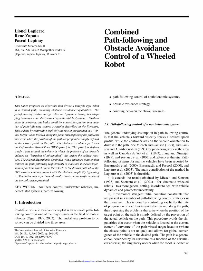
The following assumptions are made regarding the robot(see Figure 1). The vehicle, of width 2L, has two identical par-allel, non-deformable rear wheels of radius R, which are con-trolled by two independent motors, and a passive front wheel.It is assumed that the plane of each wheel is perpendicular tothe ground and that the contact between the wheels and theground is pure rolling and non-slipping, i.e. the velocity of thecenter of mass of the robot is orthogonal to the rear wheelsaxis. It is further assumed that the masses and inertias of thewheels are negligible and that the center of mass of the mobilerobot is located in the middle of the axis connecting the rear

Fig. 1. Path following: frames definition and problem posedescription.

wheels. The wheels control provides a forward force F andan angular torque N applied at the vehicle’s center of mass.The vehicle mass and moment of inertia are denoted m andI , respectively. Let u and r denote the forward and rotationalvelocity of the vehicle.

2.1.1. Kinematic equations of motion. The Serret–FrenetFrame

The solution to the problem of path following derived in Mi-caelli and Samson (1995) admits an intuitive explanation: apath-following controller should look at (i) the distance fromthe vehicle to the path and (ii) the angle between the vehiclevelocity vector and the tangent to the path, and reduce both tozero. This motivates the development of the kinematic modelof the vehicle in terms of a Serret–Frenet frame �F� that movesalong the path, with abscissa denoted s1 and ordinate y1� �F�plays the role of the body axis of a “virtual target vehicle” thatshould be tracked by the “real vehicle”. Using this set-up, theabovementioned distance and angle become the coordinates ofthe error space in which the control problem is formulated andsolved. In this paper, motivated by the work in Micaelli andSamson (1995), a Frenet frame �F� that moves along the pathto be followed is used with a significant difference: the Frenetframe is not attached to the point on the path that is closestto the vehicle. Instead, the origin of �F� along the path ismade to evolve according to a conveniently defined functionof time, effectively yielding an extra controller design parame-ter. As will be seen, this seemingly simple procedure allowsone to lift the stringent initial condition constraints that arisewith the path-following controller described in Micaelli andSamson (1993). The notation that follows is now standard.

Consider Figure 1, where P is an arbitrary point on thepath to be followed and Q is the center of mass of the mov-ing vehicle. Associated with P , consider the corresponding




Serret–Frenet frame �F�. The signed curvilinear abscissa of Palong the path is denoted s. Clearly, Q can either be expressedas q = �X� Y� 0� in a selected inertial reference frame �I� or as�s1� y1� 0� in �F�. Stated equivalently, Q can be given in �X� Y �or �s1� y1� coordinates (see Figure 1). Let the position of pointP in �I� be vector p. Let

R �

��cos � c sin � c 0

� sin � c cos � c 0

0 0 1

��be the rotation matrix from �I� to �F�, parameterized locally bythe angle � c. Define �c � �� c. Then,�� c � �� c � cc�s��s

�cc�s� � gc�s��s(1)

where cc�s� and gc�s� � dcc�s�ds denote the path curvature and

its derivative, respectively. The velocity of P with respect to�I� can be expressed in �F� to yield

dpdt

�F

�

��s0

0

�� It is also straightforward to compute the velocity of Q in �I� as

dqdt

�I

�

dpdt

�I

�R�1

drdt

�F

�R�1��c r�

where r is the vector from P to Q. Multiplying the above equa-tion on the left by R gives the velocity of Q in �I� expressed in�F� as

R

dqdt

�I

�

dpdt

�F

�

drdt

�F

��c r

Using the relations

dqdt

�I

�

��X�Y0

��

drdt

�F

�

��s1

�y1

0

�� and

�c r �

��0

0

�� cc�s��s

��

s1

y1

0

��

�

��cc�s��s y1

cc�s��ss1

0

�� equation (2) can be rewritten as

R

��X�Y0

�� s�1� cc�s�y1�� s1

�y1 � cc�s��ss1

0

�� Solving for �s1 and �y1 yields��

�s1 �

cos � c sin � c

�� X�Y

�� s �1� cc y1�

�y1 � � sin � c cos � c

�� X�Y

�� cc �ss1�

(2)

At this point it is important to notice that in Micaelli and Sam-son (1993), s1 � 0 for all t , since the location of point P isdefined by the projection of Q on the path, assuming the pro-jection is well defined. One is then forced to solve for �s in theequation above. However, by doing so 1� cc y1 appears in thedenominator, thus creating a singularity at y1 � 1

cc. As a result,

the control law derived in Micaelli and Samson (1993) requiresthat the initial position of Q be restricted to a tube aroundthe path, the radius of which must be less than 1

cc�max, where

cc�max denotes the maximum curvature of the path. Clearly,this constraint is very conservative since the occurrence of alarge cc�max in only a very small section of the path will im-pose a rather strict constraint on the initial vehicle position, nomatter where it starts with respect to that path.

By making s1 not necessarily equal to zero, a virtual targetthat is not coincident with the projection of the vehicle on thepath is created, thus introducing an extra degree of freedom forcontroller design. By specifying how fast the newly definedtarget moves, the occurrence of a singularity at y1 � 1

ccis

removed. The velocity of the unicycle in the �I� frame satisfiesthe equation �� X

�Y

�� u

�� cos �m

sin �m

�� (3)




where �m and u denote the yaw angle of the vehicle and itsbody-axis speed, respectively. Substituting (3) in (2) and in-troducing the variable � � �m � � c gives the kinematic modelof the unicycle in �s� y� coordinates as��

�s1 � ��s �1� cc y1�� u cos �

�y1 � �cc �ss1 � u sin �

�� m � cc �s(4)

where �m = ��m .

2.1.2. Dynamics. Problem Formulation

The dynamical model of the unicycle is obtained by augment-ing (4) with the equations�� u � F

�

�� m � cc s � gc �s2(5)

where ��m � N� and � and � are the mass and the moment

of inertia of the unicycle, respectively. Let FP F and NP F bethe path-following control inputs, the forward force and theangular torque, respectively.

With the above notation, the problem under study can beformulated as follows:

Given a desired speed profile ud�t� � umin � 0 for the vehiclespeed u, derive a feedback control law for FP F and NP F todrive y1, � , and u � ud asymptotically to zero.

2.2. Nonlinear Controller Design

This section introduces a nonlinear closed loop control law tosteer the dynamic model of a wheeled robot described by (4)and (5) along a desired path. Controller design builds on pre-vious work by Micaeli and samson (1993) on path-followingcontrol and relies heavily on backstepping techniques.

2.2.1. Kinematic Controller design

The analysis that follows is inspired by the work in Samsonand Ait-Abderrahim (1991) and Micaelli and Samson (1993)on path-following control for kinematic models of wheeled ro-bots. Recall from the problem definition in the previous sec-tion that the main objective of the path-following control lawis to drive y1 and � to zero. Starting at the kinematic level,these objectives can be embodied in the Lyapunov functioncandidate (Micaelli and Samson 1993).

V1 � 1

2�s2

1 � y21��

1

2�� y1� u��

2 (6)

where � is a positive gain, and it is assumed that

A.1. �y1� u� is a bounded differentiable function with respectto y1 and �0� u� � 0. This function will be called in thesequel ‘approach angle’.

A.2. y1u sin �y1� u� � 0��y �u�

A.3. lim t �u�t� �� 0�

In the V1 Lyapunov function adopted, the first term 12 �s

21 �

y21� captures the distance between the vehicle and the path,

which must be reduced to 0. The second term aims to shapethe approach angle � � �m � � c of the vehicle to the path as afunction of the ‘lateral’ distance y1 and speed u, by forcing itto follow a desired orientation profile embodied in the function. See Samson and Ait-Abderrahim (1991), where the use of a function of this kind was first proposed.

Assumption A�1� specifies that the desired relative headingvanishes as y1 goes to zero, thus imposing the condition thatthe vehicle’s main axis must be tangential to the path when thelateral distance y1 is 0. Assumption A�2� provides an adequatereference sign definition in order to drive the vehicle to thepath (turn left when the vehicle is on the right side of the path,and turn right in the other situation). Finally, Assumption A�3�states that the vehicle does not tend to a state of rest. The needfor these conditions will become apparent in the developmentthat follows. The derivative of V1 can be easily computed togive

�V1 � s1 �s1 � y1 �y1 � 1

��

� s1 �u cos � � �s �1� cc y1�� scc y1�

� y1u sin � � 1

��

� s1 �u cos � � �s�� y1u sin � 1

�

� �� y1u

sin � � sin

� � ��

Let the ideal (also called virtual) “kinematic control laws” fors and � be defined as��

�s � u cos � � k1s1�� y1u sin ��sin

��k2��

(7)

where k1 and k2 are positive gains. Then,

�V1 � �k1s21 � y1u sin � k2

�� 2�

� 0� (8)

Note the presence of the term y1u sin in the previous equa-tion and how assumption A�2� is justified.




2.2.2. Backstepping the Dynamics

The above feedback control law applies to the kinematic modelof the wheeled robot only. In what follows, using backsteppingtechniques, that control law is extended to deal with the vehicledynamics. Notice how in the kinematic design the speed of therobot u�t� was assumed to follow a desired speed profile, sayud�t�. In the dynamic design this assumption is dropped, anda feedback control law must be designed so that the trackingerror u�t��ud�t� approaches zero. Notice also that the robot’sangular speed �m was assumed to be a control input. Thisassumption will be lifted by taking into account the vehicledynamics. Following Krstic et al. (1995) define the virtualcontrol law for �� (desired behaviour of �� in (7)) as

� � � � y1usin � � sin

� � � k2�� (9)

and let � � �� be the difference between actual and desiredvalues of �� . Replacing �� by � � in the computation of �V1

gives

�V1 � �k1s21 � y1u sin � k2

�� 2�

� ��

� (10)

Augment now the candidate Lyapunov function V1 with theterms �2�2 and �u � ud�

2�2 to obtain

V2 � V1 � 1

2

��2 � �u � ud�

2�

(11)

with derivative

�V2 � �k1s21 � y1u sin � 1

�� 2

� �

1

��

�� u � ud�� u � �ud��

Simple computations show that if�� 1�� k3�

�u � �ud � k4�u � ud��(12)

where k3 and k4 are positive gains. Then

�V2 � �k1s21 � y1u sin � 1

�� 2

� k3�2 � k4�u � ud�

2 � 0� (13)

It is now straightforward to compute the control inputs F andN by solving the dynamics equation (5) to obtain�� N � � � f1�� k3 �

F � � � f2�� k4�u � ud��(14)

where �� f1�� 1�� cc s � gc �s2

f2�� ud �

The above control law makes �V2 negative semi-definite. Thisfact plays an important role in the proof of convergence of therobot to the path.

2.2.3. Choice of the Approach Angle �y1� u�

As explained before, the choice of the �y1� u� approach an-gle is instrumental in shaping the transient maneuvers duringthe path approach phase. Indeed, the approach angle is ex-pressing the desired angle to approach the path. In Micaelliand Samsion (1993), the authors propose to use �y1� u� ��sign�u� tanh�y1�. This choice is natural in the sense that alarge positive lateral distance between the robot and the path,will imply the desired relative heading robot/path to be ��2,that is the approach angle. As the robot approaches the path,and y1 diminishes, the approach angle decreases as well. Theprevious choice is intuitively justified, however, it raises somesubtle mathematical difficulties because �y1� u� is not dif-ferentiable with respect to u at u � 0. Another choice ispossible, �y1� u� � � tanh�y1u� for instance. This com-plicates the control derivation, and reduces the system per-formances in terms of convergence time. In this study, weavoid this problematic situation by imposing a forward veloc-ity ud � umin � 0 (cf. problem statement of Section 2.1.1, andthe implicit respect of the assumption A.3). As we will seelater, this condition will also be justified in the next section onobstacle avoidance (Section 3).

2.2.4. Control Expression

We now state the proposed solution for the problem exposedin Section 2.1.2.

Proposition 1: Consider the kinematic and dynamic modelsdescribed in (4) and (5). Let the approach angle �y1� u� be

�y1� u� � �sign�u��a tanh�k y1� (15)

where 0 � �a � ��2 defines the asymptotic desired approach,with k an arbitrary positive gain. Assume that ud�t� � umin �0 is a C2 function. Suppose the path to be followed is parame-terized by its curvilinear abscissa s and assume that for eachs the variables � , s1, y1, cc and gc are well defined (cf. theRemarks section below). Then, the dynamic control law��

NP F � � � f1�� k3 �

FP F � � � f2�� k4�� d��

�s � u cos � � k1s1

(16)




where the f1�� and f2�� are defines in equation (14) and k1,k2, k3, k4 and k are arbitrary positive gains, drives y1, s1 and� asymptotically to zero.

Proof: The key steps in the proof can be briefly described asfollows: let V2 be the Lyapunov function candidate expressedin equation (11). The kinematic control expression (16) yields�V2 � 0. Since �V2 is negative semi-definite and bounded be-

low, V2 is bounded and has a well defined limit. Therefore,s1, y1, � and u are bounded, since and ud are assumed to bebounded. Considering the previous equations, it is straightfor-ward to show that �s1, �y1, �� and �u are bounded as well. Directderivation allows one to compute the second derivative of V2,and prove it is bounded. Therefore, �V2 is uniformly continuousand application of Barbalat’s lemma implies that �V2 tends to 0as t tends to �. Consider now the expression for �V2 in (13).Since �V2 is a sum of negative terms and tends to 0 as t goes to�, we conclude that s1, y1, �� , �, and �u � ud� tend tozero as well. That is, the robot asymptotically converges to thepath.

Remarks: The proposed solution consists in a ‘fox–rabbit’problem where the rabbit is really cooperative since it adjustsits own velocity to help the convergence, through the expres-sion:

�s � u cos � � k1s1�

The first term u cos � is the projection of the vehicle (fox) ontothe path where the virtual target (rabbit) is located. The sec-ond term is necessary to ensure the convergence of s1 to 0,making the virtual target asymptotically converge to the clos-est point with respect to the vehicle current position. In theproblem statement, the condition ud�umin � 0 has been im-posed (implicitly covering the assumption A.3). Then the ve-hicle will not stay at rest and will effectively converge to thepath. The consequence of this is that the virtual target alsowill not stay at rest, since � and s1 are guaranteed to convergeto zero, and u � 0, for all t . Then, the path-following prob-lem, as described here can never degenerate to a pose regula-tion problem, for which Brockett’s limitations are inevitable.The assumption that the variables � , s1, y1, cc and gc are welldefined implies that there is a path parameterization that allowsone to compute the path curvature cc�s� and its spatial deriv-ative gc�s�, for all s denoting the current curvilinear abscissaof the virtual target. Moreover, this implies that the system isequipped with a sensor suite that allows computation of the ro-bot situation in the Serret–Frenet frame, i.e. the variables � , s1

and y1.

3. Obstacle Avoidance Algorithm

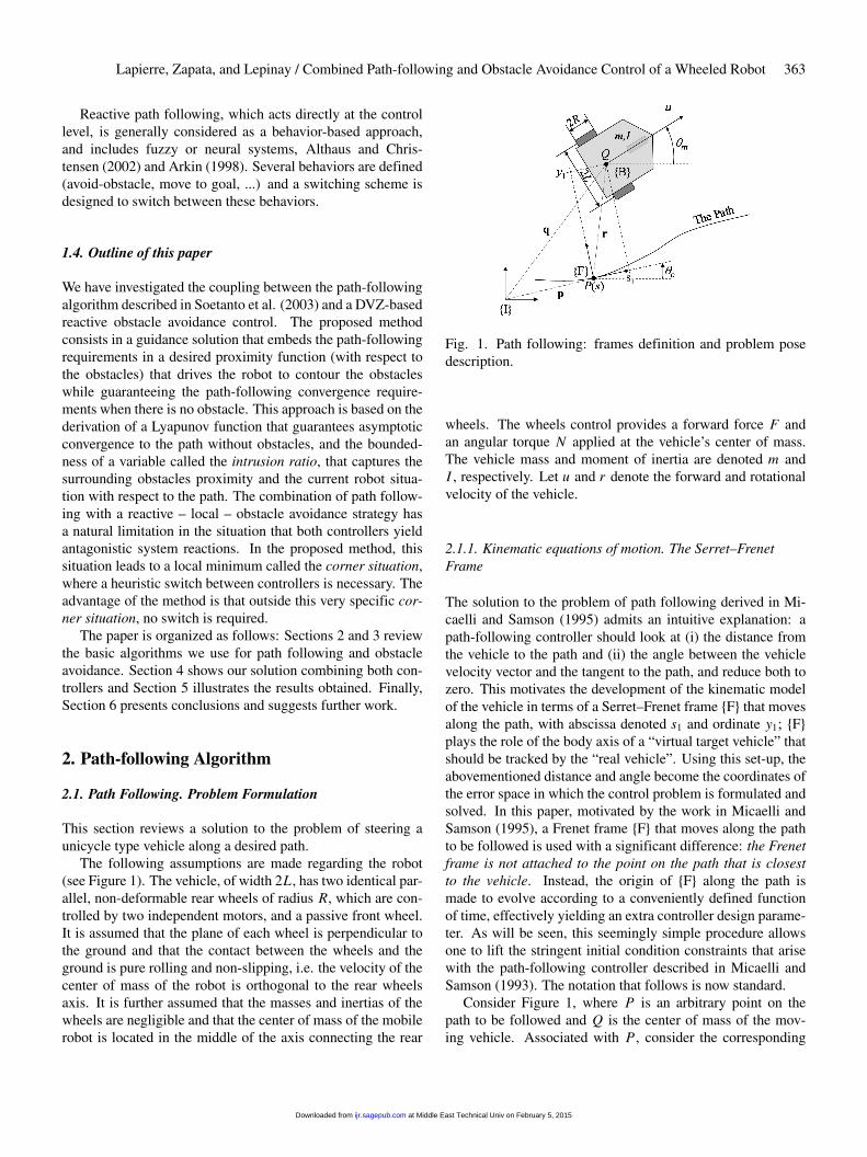
This section presents an obstacle avoidance algorithm basedon the use of a continuous Deformable Virtual Zone (DVZ).The main idea is to define the robot/environment interaction

as a DVZ surrounding the vehicle. Deformation of this riskzone � is due to the intrusion of proximity information andthus controls the robot reactions. This DVZ characterizes thedeformable zone geometry, and depends on the robot veloci-ties (forward and rotational velocities, u and r). Briefly, therisk zone, disturbed by obstacle intrusion, can be reformed byacting on the robot velocities. For a complete exposition of theDVZ principle, the reader is referred to Zapata (2004).

3.1. DVZ Principle

General statementA rigid body R representing a controlled robot is movingamong obstacles in �2. The 2-dimensional vector U � [u r]T

is the generalized momenta consisting of the translational androtational velocities of the robot. It characterizes the motionof R. Furthermore, we will assume that the robot R can becontrolled by the derivative � � �U of this vector.

Informally, we define a controlled DVZ, �h , as any DVZwhich depends on the vector U characterizing the motion ofR. This functional dependence will appear more clearly inSection 3.2, after parameterization of the DVZ:

�h � ��U�� (17)

If we let � � ��h� �� be an ordered pair of two DVZ ofR (the first one being a controlled DVZ), we define the defor-mation � of the DVZ �h with respect to � as the functionaldifference of � and �h :

� � ��h� (18)

We assume that the robot can perceive distances in all di-rections of space. We also assume that the set of maximumdistances that can be perceived by R and the set of actuallyperceived distances are also two DVZ surrounding R respec-tively named Sensor boundary and Information boundary (andrespectively denoted � and �). The deformation I of � withrespect to � is given by I � � ��.

Let �I , be a DVZ which depends on the Sensor boundarydeformation I :

�I � ��I �� (19)

The deformation � of the DVZ �h with respect to �I canbe written:

� � �I ��h � ��I �� U�� (20)

For a given point M on R, the deformation vector ��M�depends on the intrusion of proximity information I �M�, inthe rigid body workspace, and on the controlled DVZ �h .

Figure 2 shows these different DVZ.

ParameterizationEquation (20) is a functional equation that has to be parame-terized in order to be differentiable and to lead to the “usable”




Fig. 2. DVZ principle: the different DVZ for collision avoid-ance.

equation (22). For instance, it can be spatially sampled alongthe directions of the real sensors. In this case, it becomes an s-dimensional vectorial equation where s is the number of prox-imity sensors. It can also be evaluated as a polar signature andtherefore parameterized. In the case of simple mobile robots,the DVZ can be parameterized by simple shapes like ellipsoids(see 3.2).

DifferentiationBy differentiating Equation (20) with respect to time, we get:

�� U [�] � �� I [�] � (21)

where�U and� I are the differentiation operators with respectto the vectorial variables U and I . We note � � �U and � � �I .

This equation can be rewritten as:

�� A� � B�� (22)

Variations in � are controlled by a 2-fold input vectoru � [� �]T . The first control vector �, due to the robot con-troller, tends to minimize deformation of the DVZ. The secondone, � � �I , is unknown and induced by the environment it-self, the relative motion of obstacles with respect to the robotand their shapes. It can be seen as an uncontrolled input.

In the rest of the paper, we will assume that the function �relating the intrusion of information to the deformed DVZ �I

is defined as follows:

��I � �� I i f �� I � �h

0 other� ise(23)

where the sign � means the comparison of the sensor infor-mation (� � � � I ) and the undeformed DVZ �h in eachdirection of measure (see Figure 3). This restriction does notchange the principle of the DVZ and is just a simplificationleading to confusion of the intrusion I and the deformation �(their derivatives are now identical).

Fig. 3. Implementation of the function � (and projection).

3.2. The Controlled DVZ

In order to acquire an analytical expression for the polar sig-nature of the controlled DVZ, expressed in the robot framecentered on R, we consider an elliptic shape. Let P � [x y]T

be a point on the ellipse with axis cx and cy . If we assumethat the proper reference frame of the DVZ is translated fromits center by a vector a � [ax ay]T , its equation in the robotframe is given by:

x � ax

cx

�2

�

y � ay

cy

�2

� 1� (24)

The coefficients ax , ay , cx and cy are chosen heuristicallyand depend on the first component of the control vector, i.e.the general momentum u, the translational velocity of the ro-bot. We have chosen:

cx � �cx u2 � cminx

cy ��

5

3cx

ax � ��2�3�cx

ay � 0� (25)

In the direction � with respect to the main axis of the el-lipse, let dh�� be the length of the controlled DVZ �h , i.e.the norm of the vector

� R P . We can write:

� R P �

�x

y

�� cos��m� sin��m�

� sin��m� cos��m�

�� X

Y

�� (26)

where [X Y ]T are the coordinates of point P in the absoluteframe.




Using the definition of dh��

x2 � y2, we can write:�x

y

�� dh��

��1

�2

�(27)

where [�1 �2]T � [cos�� sin��]T is the unit vector in the di-rection �, expressed in the robot frame. Substituting equation(27) and equation (26) in equation (24) leads to the quadraticequation:

Adh��2 � Bdh�� C � 0 (28)

with:

A � �21c2

y cos2�� 22c2

x sin2��

B � 2ax�1c2y cos�� 2ay�2c2

x sin��

C � �ax cy�2 � �aycx�

2 � c2x c2

y � (29)

The solution of equation 28 is:

dh�� B ��B2 � 4AC

2A(30)

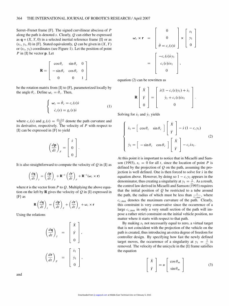
This distance clearly depends on the form parameters ofthe controlled DVZ, i.e. the coefficients ax , ay , cx and cy .Less explicitly, it also depends on the orientation of the DVZ,i.e. on the attitude �m of the robot. In order to compute thederivative of dh�� with respect to this angle �m (as we willneed below), we have to consider that the point P is fixed inthe absolute frame, leading to the dependence of vector � on�m . We have:

d�

d�m�� sin��

� cos��

�� (31)

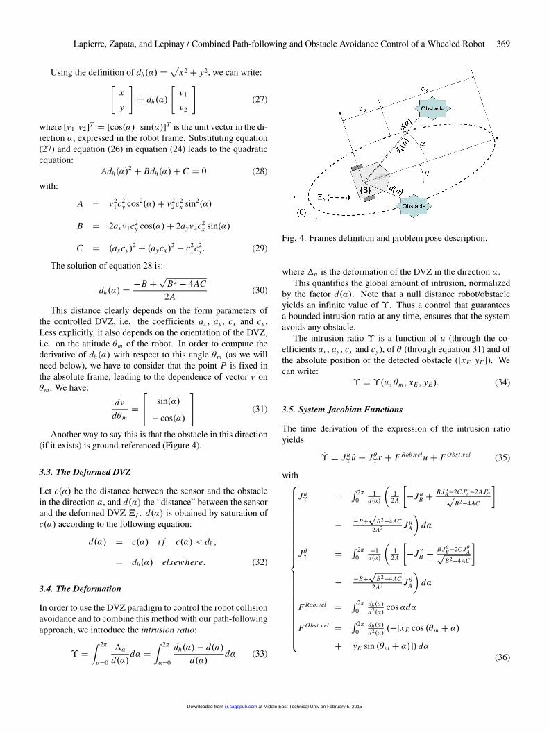
Another way to say this is that the obstacle in this direction(if it exists) is ground-referenced (Figure 4).

3.3. The Deformed DVZ

Let c�� be the distance between the sensor and the obstaclein the direction �, and d�� the “distance” between the sensorand the deformed DVZ �I . d�� is obtained by saturation ofc�� according to the following equation:

d�� c�� i f c�� dh�

� dh�� else�here� (32)

3.4. The Deformation

In order to use the DVZ paradigm to control the robot collisionavoidance and to combine this method with our path-followingapproach, we introduce the intrusion ratio:

� �� 2�

��0

��

d��d� �

� 2�

��0

dh�� d��

d��d� (33)

Fig. 4. Frames definition and problem pose description.

where �� is the deformation of the DVZ in the direction �.This quantifies the global amount of intrusion, normalized

by the factor d��. Note that a null distance robot/obstacleyields an infinite value of � . Thus a control that guaranteesa bounded intrusion ratio at any time, ensures that the systemavoids any obstacle.

The intrusion ratio � is a function of u (through the co-efficients ax , ay , cx and cy), of � (through equation 31) and ofthe absolute position of the detected obstacle ([xE yE ]). Wecan write:

� � ��u� �m� xE � yE�� (34)

3.5. System Jacobian Functions

The time derivation of the expression of the intrusion ratioyields

�� J u� �u � J ��r � F Rob��elu � F Obst��el (35)

with��

J u� � � 2�

01

d��

1

2A

��J u

B � B J uB�2C J u

A�2AJ uC�

B2�4AC

�

� �B��

B2�4AC2A2 J u

A

�d�

J �� 2�0

�1d��

1

2A

��J �B � B J�B�2C J�A�

B2�4AC

�

� �B��

B2�4AC2A2 J �A

�d�

F Rob��el � � 2�0

dh��

d2��cos�d�

F Obst��el � � 2�0

dh��

d2��[ �xE cos ��m � ��

� �yE sin ��m � ��]� d�(36)




where�� J uA � 2�cy

�cy�u cos2 �� cx

�cx�u sin2 ��

J �A � 2 cos �� sin ��c2y � c2

x�(37)

��J u

B � 2�

cos ��[c2y�ax�u � 2ax cy

�cy�u ]

� sin ��[c2x�ay�u � 2aycx

�cx�u ]�

J �B � 2�ax c2

y sin �� ayc2x cos ��

� (38)

and

J uC � 2

ax cy

�cy�ax

�u� ax

�cy

�u

�

� aycx

�cx�ay

�u� ay

�cx

�u

�

� cx cy

�cx�cy

�u� cy

�cx

�u

��(39)

and �xE � �yE define the obstacle absolute velocity. The assump-tion of static obstacles yields F Obst��el � 0. For the sake ofsimplicity, we consider only static obstacles.

3.6. Obstacle Avoidance Control Design

Consider the following Lyapunov function candidate V� � I 2

2 .The derivation yields

�V� � ��J u� �u � J ��r � F Rob��elu�� (40)

It is straightforward to see that the choice�� u � �Ku J u�� F Rob��el

Ju�

u

r � �Kr J ��(41)

where Ku� Kr are arbitrary positive gains yields �V� � 0�t .Note that tedious but straightforward computation (using forthe sake of simplicity the guidance functions in (25)) showsthat the term F Rob��el

Ju�

is a positive function that acts as a non-linear damping term. This confirms the well posedness of theexpression (41).

The control (41) is a hybrid kinematic/dynamic solution.A backstepping step is necessary for the torque control. LetVO A � 1

2 �rd � r�2 be a Lyapunov function candidate, whererd � �Kr J �� . The choice �r � �rd�Kr �r�rd� yields �VO A �0. Then the dynamic obstacle avoidance control is written as�� FO A ��

��Ku J u

�� F Rob��el

Ju�

u�

NO A � � ��rd � Kr �r � rd��(42)

where Kr and Ku are arbitrary positive gains,� and � are themass and moment of inertia of the vehicle, and rd � �Kr J �� I .

4. Combining Path-following and ObstacleAvoidance

4.1. Mathematical Inspiration

The combination of the two algorithms is solved as a guidanceproblem. The requirements are:

� the vehicle should remain far from the obstacle, i.e. inthe presence of obstacles � has to be bounded at anytime,

� when there is no obstacle, the vehicle has to asymptoti-cally converge to the desired path.

To do so, we rewrite the obstacle avoidance control, adding adesired intrusion ratio �d � Kd tanh ��d�� , where Kd

and �d are arbitrary positive gains, � and are path-followingvariables defined in the previous section (equations (4) and

(15)). Let V2 � ��d �2

2 be a Lyapunov function candidate.It is straightforward to see that the choice�� r � �Kr �� d��J �� d�� cc �s � �

�u � �Ku J u�� d�� F Rob��el

Ju�

u(43)

implies that��d asymptotically converges to a bounded setdefined as:

�� d �t � � J ��cc �s � ��Kr �J �� d�2 � Ku�J u

��2

(44)

where � �d � 2Kd�d1��d ��2 .

Note that the previous expression is bounded since �J u��

2 �0 if u �� 0,� �d is bounded and if the quantity cc �s�� is assumedto be bounded, which is covered by the assumption that the freespace is connected.

Then, following the obstacle, the vehicle cannot be driveninfinitely far from the desired path, i.e. cc �s � � remainsbounded. Moreover, if there is no obstacle, the Lyapunov func-

tion candidate degenerates to V��0 � �2d

2 , and the previouscontrol choice yields �V��0 � �Kr�

2d�

�d

2 � 0, which inducesthe path-following asymptotic convergence requirements. Thedynamic control corresponding to the previous solution is:�� FO A ��

��Ku J u

�� d�� F Rob��el

Ju�

u�

NO A � � � �rd � Kr �r � rd��(45)

where rd � �Kr �� d��J �� d� � cc �s � �, Ku and Kr

are arbitrary positive gains. At this stage one should note thatthis solution does not prevent the forward velocity u from be-ing null, and thus a poor convergence rate around the path.We therefore propose another control version that avoids thesedrawbacks, but also loses any mathematical proof of conver-gence.




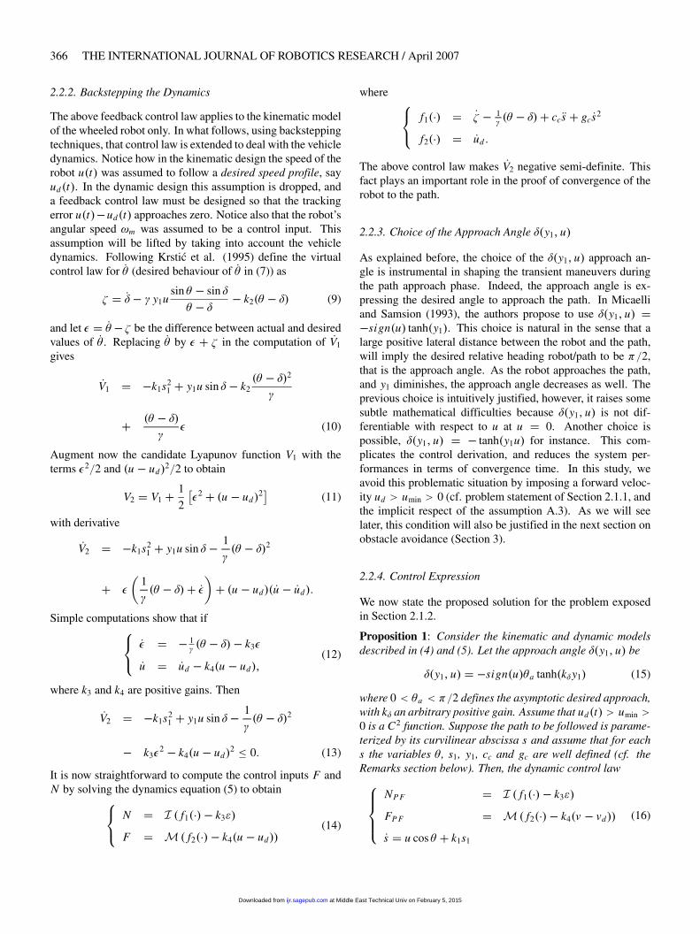
Table 1. Corner situation.

a) Corner situation b) Extract. from Corner Sit.

c) Evolut. forward vel. d) Evolut. of the ‘rabbit’.

4.2. Practical Solution

The combination of path following and obstacle avoidance ca-pabilities has a natural limitation in situations where both cri-teria induce antagonist system reactions.

For instance, the obstacle avoidance algorithm may demandthat the forward velocity be reduced to zero or a negative value.

This situation occurs when the deformed DVZ � is sym-metric with respect to the forward velocity direction. Then therobot will orient itself to minimize the intrusion, and regulateits forward velocity to reshape the nominal DVZ �h in orderto respect the intrusion requirement, i.e. limt �� d .This situation is called a corner situation, as described in Ta-ble 1. To avoid this problematic local minimum, the followingswitching scheme was designed. Let �l and �r be the intru-sion ratios on the left (0 � � � �) and right (� � � � 2�)side, respectively, and umin � 0 the lowest admissible for-ward velocity. The chosen corner situation detection is madewith the following switching condition. The Boolean variableC O RN E R is initialized to zero, then

i f [��l�r � 0�&�u � umin�] �C O RN E R � 1�i f ��l�r � 0� �C O RN E R � 0�� (46)

The reaction to this situation is to:

(i) reduce the forward velocity,

(ii) rotate until the obstacle is present only on one side, us-ing the following controllers.

�uC O RN E R � �Kuu

rC O RN E R � rC sign��d� (47)

where Ku is a positive gain, and rC the chosen rotationalvelocity to operate the corner extraction.

The overall control algorithm is written

i f �C O RN E R � 0�

�N � NO A � f ��NP F � F � FO A � f ��FP F�else

�N � � ��Kr �r � rC O RN E R�� F �� uC O RN E R� (48)

where the selection function is f �� 11�K��

, with KI a pos-itive gain. Note that this algorithm causes the robot to travel




with a positive forward velocity u � umin � 0, outside thecorner situation. This guarantees the well posedness of theexpressions (43), (44) and (45). Then the global control (48) iswell posed in any situation. Table 1(c) describes the evolutionof the forward velocity while encountering a corner situation.The increase in the intrusion ratio induces a decreasing for-ward velocity, down to umin � 0�2m�s�1, while the obstacleis present on the left and right side of the robot (�l�r � 0).The robot is then controlled according to (47), where rcorner isdriven by the sign of �d . This allows the system to be drivenaway from the path, thus guaranteeing the system skirts theobstacle. Table 1(d) shows the evolution of the virtual target(‘rabbit’) along the path, where its backward movement to-wards the closest point on the path is seen, while the robot isskirting the obstacle.

5. Results

The previous solution implicitly requires an estimation of ��in the computation of FO A. The numerical derivation of thesensor information induces noise amplification and will notprovide an accurate estimation of �� . Therefore, we degradethe previous solution at a kinematic level, that does not requirethe estimation of �� . Moreover, the considered robot (cf. Fig-ure 5) accepts as control inputs the desired velocities u and r ,and its rapid actuator response (combined with its light massand inertia) allows implementation of a kinematic controllerwithout degrading the overall performance.�� r � rO A � f ��rp f

u � uO A � f ��u pf

(49)

where��

rP F � � � K P Fr �� cc �s

u P F �� t

0 � �ud � K P Fu �u � ud��dt

�s � u cos � � kss1

rO A � �K O Ar �� d��Jr �� d�� cc �s � �

uO A �� t

0 ��K O Au J�u �� d�� Frob��el

J�uu�dt�

(50)

The DVZ guidance functions are chosen according to (25).The other functions are chosen according to the followingdefinitions: �� d � Kd tanh�d��

f �� 11�K��

(51)

Table 2. The chosen control parameters.

K P Fr � 0�1 K P F

u � 1 K O Ar � 0�01 K O A

u � 0�1

Kd � 10 �d � 0�01 KI � 100 ud � 1

�cx � 100 cminx � 10 K C O RN E R

u � 0�1 rc � 1

5.1. Simulation Results

We have implemented the algorithm on a unicycle simulatordeveloped with Matlab. The control parameters are chosenaccording to Table 2. The results are displayed in Table 3.Table 2(a) shows the path and obstacles definitions. The ro-bot is of the unicycle type, on which a 32-proximity-sensorsbelt is mounted, displayed as surrounding radial rays of lengthdefined by the nominal DVZ. Table 2(b) indicates a corner sit-uation, in which we see the reduction of the DVZ due to thedecreased forward velocity. Table 2(c) shows the system afterthe switch from corner situation to nominal control. Finally,Table 3(d) displays the global trajectory the system has made.

5.2. Experimental Results

We have implemented the control algorithm of equations (49)on the Pekee robot from the Wany company. This robot isdriven by two independent wheels and carries a 16-infrared-proximity- sensors belt, see figure 5, and is controlled via aMitsubishi M16C family micro-controller. The complete algo-rithm, equations (49), was first implemented on an embeddedPC daughterboard, and the test results are displayed in Figure6 describing the odometric trajectory of the robot. Since thenavigation system is based only on odometric information, thereal trajectory is not significant in the demonstration of the va-lidity of our approach. The robot clearly avoids the obstacleand returns to the nominal path without requiring switchingcontrol. This is valid in this particular situation where the cor-ner situation does not occur. Some chattering behavior hasto be filtered out by gain tuning according to the Pekee ro-bot capabilities. Figure 7 shows the evolution of the forwardvelocity. The black dots denote the desired velocity when noobstacle is detected, the stars indicates the evolution of the for-ward velocity in the presence of obstacles. A second stageconsisted in simplifying the algorithm complexity (includingtrigonometric look-up tables) in order to reduce the compu-tational burden, and implementation of the solution directlyon the M16C micro-controller onboard the vehicle. The testsdisplayed similar vehicle behavior, since the sensor (US andodometry) accuracy did not allow demonstration of the reac-tivity benefits of the low level implementation.




Table 3. Simulation results.

a) Path and Obst. Def. b) Corner Situation

c) Extract. from Corner Sit. d) Final Trajectory

Fig. 5. The Wany robot “Pekee”.

6. Conclusions

We have designed a combined path following and obstacleavoidance control law for a unicycle type robot based on theuse of the DVZ concept and on a Lyapunov and backsteppingdesign. Implementation of this solution on the Wany robot“Pekee” illustrates an interesting performance, avoiding un-necessary hot switches when the vehicle travels with an im-

portant forward velocity. With this system, we combine thereactivity of the DVZ principle with a path-following controlwithout requiring any path replanning. The next step in thisstudy is to intrinsically attribute the reactivity of the guidancesystem to the path-following virtual target, explicitly control-ling the evolution of an added virtual state of the virtual target,along the y1 direction (see Figure 1). Then the main robotcontrol could be designed as a tracker of a cooperative virtualtarget� note that the system reactivity is then in charge of a newdynamic guidance system.

Acknowledgements

This work is supported by a post doctoral grant from theFrench national RNTL project WACIF. For further infor-mation on this project, please contact http://intranet.wacif.net/default.aspx .




Fig. 6. Experimental results, trajectories.

Fig. 7. Experimental results, forward velocity.




References

Aicardi, M., Casalino, G., Bicchi, A., and Balestrino, A.(1995). A closed loop steering of unicycle-like vehiclesvia Lyapunov techniques. IEEE Robotics and AutomationMagazine, March, 27–35.

Aicardi, M., Casalino, G., Indiveri, G., Aguiar, P., Encarnacao,P. and Pascoal, A. (201). A planar path following con-troller for underactuated marine vehicles. Proceedings ofMED’2001, Dubrovnik, Croatia, June.

Althaus, P. and Christensen, H. (2002). Behavior coordinationfor navigation in office environment, IEEE/RSJ Interna-tional Conference on Intelligent Robots and Systems, Lau-sanne, Switzerland, October.

Arkin, R. C. (1998). Behavior Based Robotics. MIT Press,Cambridge, MA.

Canudas de Wit, C., Khennouf, H., Samson, C., and Sordalen,O. J. (1993). Nonlinear control design for mobile robots.In Recent Trends in Mobile Robotics (eds Y. F. Zheng), Vol11, pp.121–156, World Scientific Series in Robotics andAutomated Systems. 1993

Elnagar, A. and Hussein, A. (2002). Motion planning usingMaxwell’s equations. IEEE/RSJ International Conferenceon Intelligent Robots and Systems, Lausanne, Switzerland,October.

Encarnação, P., Pascoal, A., and Arcak, M. (2000). Path fol-lowing for marine vehicles in the presence of unknown cur-rents. Proceedings of SYROCO’2000, 6th IFAC Symposiumon Robot Control, Vienna, Austria.

Encarnação, P. and Pascoal, A. (2000). 3D path follow-ing for autonomous underwater vehicle. Proceedings ofCDC’2000, 39th IEEE Conference on Decision and Con-trol, Sydney, Australia.

Fierro, R. and Lewis, F. (1997). Control of a nonholo-nomic mobile robot: backstepping kinematics into dynam-ics. Journal of Robotic Systems, 14(3): 149–163.

Ge, S. and Cui, Y. (2000). Path planning for mobile robotsusing new potential functions. Proceedings of the 3rd AsianControl Conference, Shangai, China, July.

Iniguez, P. and Rossel, J. (2002). A hierarchical and dynamicmethod to compute harmonic functions for constrained mo-tion planning. IEEE/RSJ International Conference on Intel-ligent Robots and Systems, Lausanne,Switzerland, October.

Jiang, Z. P. and Nijmeijer, H. (1999). A recursive techniquefor tracking control of nonholonomic systems in chainedform. IEEE Transactions on Robotics and Automation,44(2): 265–279.

Krstic, M. I., Kanellakopoulos, and Kokotovic, P. (1995). Non-linear and Adaptive Control Design. John Wiley & Sons,Inc., New York.

Lapierre, L., Soetanto, D., and Pascoal, A. (2003). Nonlin-ear path following with application to the control of au-tonomous underwater vehicle. CDC 2003, 42nd IEEE Con-ference on Decision and Control, Maui, Hawaii, USA, De-cember.

Louste, C. (1999). Conception d’une methode de planificationpour robot mobile selon la methode des milieux continusappliquee aux fluides visqueux. PhD thesis no. 6701,LIRMM, Montpellier, France.

Micaelli, A. and Samson, C. (1993). Trajectory-trackingfor unicycle-type and two-steering-wheels mobile robots.Technical Report No. 2097, INRIA, Sophia-Antipolis, No-vember.

Ogren, P. (1989). Real-time obstacle avoidance for fast mobilerobots. IEEE Transactions on Systems, Man and Cybernet-ics, 19(5): 1179–1187.

Ogren, P. and Leonard, N. (2002). A provable convergent dy-namic window approach to obstacle avoidance. IFAC WorldCongress, Barcelona, Spain, July.

Ogren, P. (2003). Formation and Obstacle Avoidance in Mo-bile Robot Control. PhD thesis, Stockholm, Norway, June.

Rimon, E. and Koditschek, D. (1992). Exact robot navigationusing artificial potential functions. IEEE Transactions onRobotics and Automation, 8(5): 501–518.

Samson, C. and Ait-Abderrahim, K. (1991). Mobile robot con-trol Part 1: Feedback control of a non-holonomic mobile ro-bot. Technical Report No. 1281, INRIA, Sophia-Antipolis,France, June.

Soetanto, D., Lapierre, L., and Pascoal, A. (2003). Adaptive,nonsingular path following control of dynamic wheeled ro-bot. CDC’03, 42nd IEEE Conference on Decision and Con-trol, Maui, Hawaii, USA, December.

Zapata, R., Cacitti, A., and Lepinay, P. (2004). DVZ-basedcollision avoidance control of non-holonomic mobile ma-nipulators. European Journal of Automated Systems, 38(5):559–588.



the international journal of robotics research-2007-lapierre-361-75

Documents