the international journal of robotics research · the international journal of ... multimedia...

http://ijr.sagepub.com/

Robotics ResearchThe International Journal of

http://ijr.sagepub.com/content/29/12/1475The online version of this article can be found at:

DOI: 10.1177/0278364910377243

2010 29: 1475 originally published online 9 August 2010The International Journal of Robotics ResearchRyan N. Smith, Yi Chao, Peggy P. Li, David A. Caron, Burton H. Jones and Gaurav S. Sukhatme

Processes Based on Predictions from a Regional Ocean ModelPlanning and Implementing Trajectories for Autonomous Underwater Vehicles to Track Evolving Ocean

Published by:

http://www.sagepublications.com

On behalf of:

Multimedia Archives

can be found at:The International Journal of Robotics ResearchAdditional services and information for

http://ijr.sagepub.com/cgi/alertsEmail Alerts:

http://ijr.sagepub.com/subscriptionsSubscriptions:

http://www.sagepub.com/journalsReprints.navReprints:

http://www.sagepub.com/journalsPermissions.navPermissions:

http://ijr.sagepub.com/content/29/12/1475.refs.htmlCitations:

at UNIV OF SOUTHERN CALIFORNIA on November 17, 2010ijr.sagepub.comDownloaded from


http://ijr.sagepub.com/content/29/12/1475

http://www.sagepublications.com

http://www.ijrr.org/

http://ijr.sagepub.com/cgi/alerts

http://ijr.sagepub.com/subscriptions

http://www.sagepub.com/journalsReprints.nav

http://www.sagepub.com/journalsPermissions.nav

http://ijr.sagepub.com/content/29/12/1475.refs.html


Planning and Implementing Trajectoriesfor Autonomous Underwater Vehicles toTrack Evolving Ocean Processes Basedon Predictions from a Regional OceanModel

The International Journal ofRobotics Research29(12) 1475–1497©The Author(s) 2010Reprints and permission:sagepub.co.uk/journalsPermissions.navDOI: 10.1177/0278364910377243ijr.sagepub.com

Ryan N. Smith1, Yi Chao2, Peggy P. Li2, David A. Caron3, Burton H. Jones3 andGaurav S. Sukhatme1

AbstractPath planning and trajectory design for autonomous underwater vehicles (AUVs) is of great importance to theoceanographic research community because automated data collection is becoming more prevalent. Intelligent planningis required to maneuver a vehicle to high-valued locations to perform data collection. In this paper, we present algorithmsthat determine paths for AUVs to track evolving features of interest in the ocean by considering the output of predictiveocean models. While traversing the computed path, the vehicle provides near-real-time, in situ measurements back to themodel, with the intent to increase the skill of future predictions in the local region. The results presented here extend prelim-inary developments of the path planning portion of an end-to-end autonomous prediction and tasking system for aquatic,mobile sensor networks. This extension is the incorporation of multiple vehicles to track the centroid and the boundary ofthe extent of a feature of interest. Similar algorithms to those presented here are under development to consider additionallocations for multiple types of features. The primary focus here is on algorithm development utilizing model predictionsto assist in solving the motion planning problem of steering an AUV to high-valued locations, with respect to the datadesired. We discuss the design technique to generate the paths, present simulation results and provide experimental datafrom field deployments for tracking dynamic features by use of an AUV in the Southern California coastal ocean.

KeywordsAlgal bloom, autonomous glider, autonomous underwater vehicles, feature tracking, ocean model predictions, pathplanning

1. Introduction

Coastal ocean regions are dynamic and complex environ-ments that are driven by an intricate interaction betweenatmospheric, oceanographic, estuarine/riverine and land–sea processes. Effective observation and quantification ofthese processes requires the simultaneous measurement ofdiverse water properties to capture the spatial and temporalvariability. The implementation of multiple and adaptablesensors can facilitate simultaneous and rapid measure-ments that capture the appropriate scale of spatiotemporalvariability for many of the phenomena that we seek tounderstand occurring in the coastal ocean. Autonomousunderwater vehicles (AUVs) are a key tool in this effective,efficient and adaptive data collection procedure to improveour overall understanding of coastal processes and ourworld’s oceans. Through development of these intelligentsystems, scientists can implement continuous monitoringand sampling programs that provide fine-scale resolutionfar surpassing previous sampling methods, such as infre-quent measurements from ships, buoys and drifters. One

example of intelligent ocean sampling is the coordinatedcontrol of autonomous and Lagrangian platforms and sen-sors (ALPS), developed in the series of articles Fiorelli et al.(2006), Leonard et al. (2007), and Paley et al. (2007, 2008).Such research efforts have opened the door for the designand implementation of adaptive, mobile sensor platformsand networks to aid in the study of complex phenomenasuch as ocean currents, tidal mixing and other dynamicocean processes.

1 Robotic Embedded Systems Laboratory, University of SouthernCalifornia, Los Angeles, CA 90089, USA

2 Jet Propulsion Laboratory, California Institute of Technology, 4800 OakGrove Drive, Pasadena, CA 91109, USA

3 Department of Biological Sciences, University of Southern California,Los Angeles, CA 90089, USA

Corresponding author:Ryan N SmithRobotic Embedded Systems LaboratoryUniversity of Southern CaliforniaLos Angeles, CA 90089USAEmail: [email protected]



1476 The International Journal of Robotics Research 29(12)

To this end, three laboratories at the University of South-ern California (USC) have formed CINAPS (pronounced[sin-aps]); the Center for Integrated Networked AquaticPlatforms. The mission of this collaborative research groupis to bridge the gap between technology, communicationand the scientific exploration of local and regional aquaticecosystems through the implementation of an embeddedsensor network along the Southern California coast (Smithet al. 2010a). This infrastructure is designed for facilita-tion of long-term, in-depth, multi-faceted investigation ofphysical, chemical and biological processes resulting fromcoastal urbanization and climate change. One componentof this network, and the focus of this paper, are mobilesensor platforms in the form of autonomous Slocum gliders(gliders) (Webb Research Corporation 2008). Based ontheir deployment longevity, and the use of multiple gliders(see e.g. Davis et al. (2008)), these vehicles can provide anextended spatiotemporal series of observations (see detailsin Section 4). This study investigates a path planningmethod for a multi-vehicle application for gliders in theSouthern California coastal ocean.

The path planning method presented here is based uponpredictions from a regional ocean model. As complex andunderstudied as the ocean may be, we are able to modeland predict certain behaviors moderately well over shorttime periods. Consistently comparing model predictionswith collected data, and adjusting for discrepancies, willincrease the range of validity of existing ocean models, bothtemporally and spatially.

Utilizing available technology and infrastructure, weconsider the problem of integrating ocean model predic-tions into the path planning and trajectory design procedurefor AUVs, with the goal of tracking and sampling within aninteresting and evolving ocean feature. Collecting data forocean science can be extremely hit-or-miss, both temporallyand spatially, especially when one is interested in a spe-cific biogeochemical event. In addition, areas of scientificinterest within the ocean dynamically move and evolve.Thus, continuously operating a sensor platform (static ormobile) in a predesignated and confined sampling area isnot the most effective technique to gather data for analysisand assessment of ocean processes which may occur spo-radically, and dynamically propagate throughout the ocean.Here we aim to increase the likelihood of gathering dataof high scientific merit, i.e. data of great importance tounderstanding the feature of interest, by deriving the sam-pling locations from a prediction of the evolution of a givenfeature of interest. We build upon the three-dimensional(two spatial dimensions plus time), single-vehicle algorithmpresented in Smith et al. (2009a), with the intention ofgenerating a mission plan that accurately steers multiplegliders to locations of high value within an evolving oceanfeature. The primary contributions of this paper are thedevelopment of an innovative toolchain, and the waypoint-generation algorithms for the practical application of AUVpath planning and trajectory design.

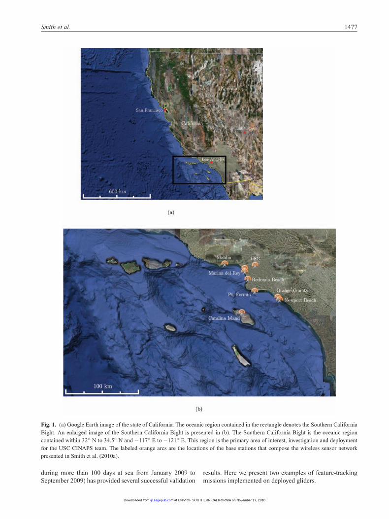
The goal of this study is to present an innovative oceansampling method that utilizes model predictions and glidersto collect scientifically interesting oceanographic data thatcan also increase the predictive skill of a model. Ourmotivation is to track and collect daily information aboutan ocean process or feature which has a lifespan on theorder of weeks. Based on the interesting biogeochemicalocean dynamics presented in Section 2, in addition to itsproximity to our laboratories at USC, we choose to focusour research on an oceanographic region referred to as theSouthern California Bight (SCB)1. The regional locationof the SCB is denoted by the box in Figure 1(a), with anenlarged view of the SCB presented in Figure 1(b).

The mission plan to track and monitor dynamicallyevolving ocean processes or features is iteratively generatedas follows. First, we identify a feature of interest in the SCBvia direct observation or through remotely sensed data (e.g.satellite imagery). We then use a regional ocean model topredict the behavior of this feature, e.g. outfall from a wastewater treatment plant, over a short time period, such as oneday. This prediction is used to generate a sampling planfor deployed glider(s) that steer the vehicle(s) to regionsof scientific interest, based upon the given feature and itspredicted evolution. Throughout execution of the samplingplan, collected data are transmitted via an embeddedwireless network (Pereira et al. 2009; Smith et al. 2009b),and assimilated into the ocean model. Incorporating thisin situ ground truth, a new prediction is generated by themodel. This entire process is repeated until the featuredissipates or is no longer of interest.

We begin our discussion with a description of theprimary research focus related to this study, a harmfulalgal bloom (HAB). An algal bloom, and in particular aHAB, is a rapid increase of biomass of phytoplankton orcyanobacteria (potentially toxin producing species) causedby the addition of nutrients to and/or an alteration inthe chemical properties of the ocean. Nutrients can beadded to the coastal ocean via river runoff or waste wateroutfalls. Ocean chemistry can be altered by the addition offreshwater from these events, as well as by ocean processessuch as an eddy or upwelling.

We continue our discussion with definitions of thesensor platform and ocean model considered, and a reviewof previous work related to similar problems. Section5 contains an in-depth discussion and statement of thepath planning problem, and describes the two mainalgorithms designed to obtain the waypoints that define ourpath. Here we present a waypoint-selection algorithm forboth a boundary-tracking and a centroid-tracking missionscenario. We design sampling plans and present simulatedand implemented experimental results for AUV retaskingin Southern California coastal waters. We conclude withan analysis of the experimental results and present areasof ongoing and future investigation. A crucial componentto this study is the validation of this toolchain via at-seatrials. Extensive deployment time (>1, 500 km traversed



Smith et al. 1477

Fig. 1. (a) Google Earth image of the state of California. The oceanic region contained in the rectangle denotes the Southern CaliforniaBight. An enlarged image of the Southern California Bight is presented in (b). The Southern California Bight is the oceanic regioncontained within 32◦ N to 34.5◦ N and −117◦ E to −121◦ E. This region is the primary area of interest, investigation and deploymentfor the USC CINAPS team. The labeled orange arcs are the locations of the base stations that compose the wireless sensor networkpresented in Smith et al. (2010a).

during more than 100 days at sea from January 2009 toSeptember 2009) has provided several successful validation

results. Here we present two examples of feature-trackingmissions implemented on deployed gliders.




2. Background and Motivation

2.1. Southern California Ocean Dynamics

The motivation for using predictive capabilities to designtrajectories with the intent of tracking an evolving oceanfeature is derived from a practical problem that existsin many coastal communities around the world, and, inparticular, Southern California. As the rate of urbanizationin coastal communities continues to increase, land use andland cover (i.e. significant increase in impervious surfaces)in these areas are permanently altered. This alterationaffects both the quantity of freshwater runoff, and itsparticulate and solute loadings, which has an unknownimpact (physically, biogeochemically, biologically andecologically) on the coastal ocean (Warrick and Fong 2004).One documented result of these impacts is an increase inthe occurrence of algal and phytoplankton blooms. Suchbiological phenomena are a primary research interest of theauthors. In particular, we are interested in the assessment,evolution and potential prediction of algal blooms that havethe potential to include harmful algal species (i.e. harmfulalgal blooms (HABs)). The environmental triggers leadingto the onset, evolution and dissemination of HAB events arewidely unknown and are under active investigation.

Given the ecological and socio-economic importance ofcoastal regions, like Southern California (U.S. Commissionon Ocean Policy 2004), it is important to be able toaccurately assess, and ultimately predict, how changesdriven by urbanization and climate impact these areas.

In addition to regional anthropogenic disturbances,Southern California experiences significant decadal andinterannual variability associated with the Pacific decadaloscillation (PDO) and the El Niño southern oscillation(ENSO) (Dailey et al. 1993; Kennedy et al. 2002). Theseclimatic phenomena impact the frequency and intensityof the regional episodic storm events, as well as thephysical and biogeochemical dynamics of the coastalmarine ecosystem. The increased rainfall in an urban,coastal region results in freshening of sea-surface watersthrough direct rainfall into the ocean and from freshwaterinflow at the coastal boundary from streams and rivers.The river runoff supplies nutrient-rich waters to the oceansurface, which may lead to a bloom of photosyntheticorganisms (i.e. algal bloom).

An open question in coastal ocean science is to dissem-inate whether or not we can distinguish anthropogenicallyaffected processes from natural variations and effects. Theability to track and monitor evolving features resulting fromanthropogenic inputs can help answer this question and oth-ers related to the increased urbanization of coastal regions.

2.2. Harmful Algal Blooms

Microscopic organisms are the base of the food chainand are what all aquatic life ultimately depends upon forfood. There are a few dozen species of phytoplankton andcyanobacteria that can create potent toxins when provided

with the right conditions. These harmful algae can causeharm via toxin production, or by their accumulated biomasswhich may affect levels of dissolved oxygen in the water.Impacts to humans from HABs include, but are not limitedto, severe illness and potential death following consumptionof, or indirect exposure to, HAB toxins. In addition, coastalcommunities and commercial fisheries can suffer severeeconomic losses due to fish, bird and mammal mortalities,and decrease in tourism due to beach closures. For thesereasons, it is of interest to predict when and where HABsmay form and which coastal areas they may affect. Forgeneral information on HABs, we refer the interested readerto Anderson (2008). Harmful algal blooms are an activearea of research on all coasts of the United States, andare of large concern for coastal communities in SouthernCalifornia (Schnetzer et al. 2007).

A related threat of HABs deals with the sinkingof Pseudonitzschia, i.e. transfer of toxicity to the seafloor, as discussed in Wood et al. (2009). Autonomousgliders have been used recently during the North AtlanticBloom experiment to track the sinking of primaryproduction from the surface to 800–1,000 m (Gray et al.2008). It is of interest to document the sinking ofthe Pseudonitzschia biomass to determine the harmfuleffects away from the surface. Vertical movement oraggregation at specific depths can also be important factorsaffecting the abundance of some harmful algae such asdinoflagellates and their associated toxins (Kudela et al.2008). Marine biologists are interested in defining thevertical zonation and migratory patterns of a dinoflagellate,and the interactions of the organism with physical processesof the ocean (e.g. currents, shear, density gradients, light)and the chemical structure (e.g. nutrients). Hence, withtheir unique sawtooth-shaped trajectories, gliders are a goodcandidate platform to study surface blooms as well as theirvertical migration.

Motivated by the number of problems linked to HABs,and algal blooms in general, it is of interest to studyocean features that can potentially promote a bloom event.In particular, blooms are likely to occur when nutrient-rich waters are brought to the surface. Ocean processesand features of interest promoting these conditions arecold-core eddys, upwelling, river runoff and waste wateroutfalls. These events alter the biochemical compositionof the surrounding water, and provide the excessnutrients to support higher productivity and a bloom ofmicroorganisms.

From the coastal dynamics and rapid urbanization inSouthern California coastal communities discussed earlier,we choose plumes from river runoff and waste water outfallsas features to track and monitor. Both of these events canbe discretely quantified; river runoff happens after a stormevent and most waste water outfalls are human controlled.Hence, we have a good idea of when and where a plume willbe present in the SCB, and can employ the proper meansto detect its onset and evolution. Henceforth, we will referto a feature of interest to be tracked as a plume, which is



Smith et al. 1479

understood to encompass freshwater plumes, waste wateroutfalls and algal blooms.

The density of the considered plumes is less than thesurrounding sea water, and forms a lens on the surface.The movements of these plumes are dominated by surfacecurrents and local winds. The focus of this paper is ontracking the movement of plumes through the ocean byuse of predictive tools and gliders to study the factors andconditions leading to the onset and lifespan of a HAB event.We remark that similar techniques to those presented herecan be applied to study eddys and upwelling; however,with the choice taken here, we increase the likelihoodof catching an actual event upon which to implementthis innovative technology toolchain and trajectory designmethod.

3. Regional Ocean Modeling System

The predictive tool utilized in this study is the regionalocean model system (ROMS) – a split-explicit, free-surface, topography-following-coordinate oceanic model.ROMS is an open-source, ocean model that is widelyaccepted and supported throughout the oceanographic andmodeling communities. Additionally, the model was devel-oped to study ocean processes along the western U.S. coast,which is our primary area of study. The model solvesthe primitive equations using the Boussinesq and hydro-static approximations in vertical sigma (i.e. topography-following) and horizontal orthogonal curvilinear coordi-nates. ROMS uses innovative algorithms for advection,mixing, pressure gradient, vertical-mode coupling, timestepping and parallel efficiency. Detailed information onROMS can be found in Shchepetkin and McWilliams(1998, 2005).

The version of ROMS used in this study is compiledand run by the Jet Propulsion Laboratory (JPL), CaliforniaInstitute of Technology, and provides hindcasts, nowcastsand hourly forecasts (up to 36 h) for the SCB via a webinterface (Vu 2008) or via access to their THREDDSdata server (Jet Propulsion Laboratory 2009). The JPLversion of ROMS (see e.g. Chao et al. (2008) and Liet al. (2008a,b)) assimilates HF radar surface currentmeasurements, data from moorings, satellite data and anydata available from sensor platforms located or operatingwithin the model boundary.

This model utilizes a nested configuration, withincreasing resolution covering the U.S. western coastalocean at 15 km, the Southern California coastal oceanat 5 km and the SCB at 1 km. In addition to the 1 kmoutput, a resampled 2.2 km resolution output, correlatedto the assimilated HF radar grid resolution, is produced.The computations and predictions presented here use this2.2 km resolution product.

The interaction with JPL related to this research andROMS improvement is a two-way street. We need thepredictions to design efficient, effective and innovative

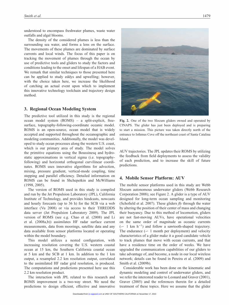
Fig. 2. One of the two Slocum gliders owned and operated byCINAPS. The glider has just been deployed and is preparingto start a mission. This picture was taken directly north of theentrance to Isthmus Cove off the northeast coast of Santa CatalinaIsland.

AUV trajectories. The JPL updates their ROMS by utilizingthe feedback from field deployments to assess the validityof each prediction, and to increase the skill of futurepredictions.

4. Mobile Sensor Platform: AUV

The mobile sensor platforms used in this study are WebbSlocum autonomous underwater gliders (Webb ResearchCorporation 2008); see Figure 2. A glider is a type of AUVdesigned for long-term ocean sampling and monitoring(Schofield et al. 2007). These gliders fly through the waterby altering the position of their center of mass and changingtheir buoyancy. Due to this method of locomotion, glidersare not fast-moving AUVs, have operational velocitieson the same order of magnitude as oceanic currents(� 1 km h−1) and follow a sawtooth-shaped trajectory.The endurance (� 1 month per deployment) and velocitycharacteristics of a glider make it a good candidate vehicleto track plumes that move with ocean currents, and thathave a residence time on the order of weeks. We haveupgraded the communication capabilities of our gliders totake advantage of, and become, a node in our local wirelessnetwork; details can be found in Pereira et al. (2009) andSmith et al. (2009b).

Considerable work has been done on the kinematic anddynamic modeling and control of underwater gliders, andwe refer the interested reader to Leonard and Graver (2001),Graver (2005) and the references therein for a detailedtreatment of these topics. Here we assume that the glider




can successfully navigate from one location to another.This is a non-trivial assumption due to the complexity ofthe underwater environment and the forces experiencedby an AUV while underway. An entire body of researchexists that is dedicated to accurate and precise executionof prescribed missions by AUVs, and is outside the scopeof the work presented here. In relation to this work,research is active to improve the navigational accuracyof our gliders by use of ROMS predictions in the SCB;see Smith et al. (2010b,c).

Briefly, an example mission for a standard glider consistsof a set maximum depth along with an ordered list ofgeographical waypoints (W1, . . . , Wn). An exact path ortrajectory connecting these locations is not prescribed bythe operator, nor are the controls to realize the finaldestination. When navigating to a new waypoint, thepresent location L of the vehicle is compared with thenext prescribed waypoint in the mission file (Wi), and theon-board computer computes a bearing and a range forexecution of the next segment of the mission. We will referto the geographical location at the extent of the computedbearing and range from L to be the aiming point Ai.The vehicle then dead reckons with the computed bearingand range towards Ai with the intent of surfacing at Wi.The glider operates under closed-loop heading and pitchcontrol only. Thus, the computed bearing is not altered,and the glider must surface to make any corrections ormodifications to its trajectory. When the glider completesthe computed segment (i.e. determines that it has traveledthe requested range at the specified bearing), it surfacesand acquires a GPS fix. Regardless of where the vehiclesurfaces, waypoint Wi is determined to be achieved. Thegeographical positional error between the actual surfacinglocation and Wi is computed, and any error betweenthese two is fully attributed to environmental disturbances(i.e. ocean currents). A depth-averaged current vector iscomputed, and this is considered when computing the rangeand bearing to Wi+1, the next waypoint in the mission list.Hence, Ai is in general not in the same physical locationas Wi. The offset between Ai and Wi is determined bythe average velocity and the perceived current experiencedduring the previous segment.

5. Problem Outline and Path Planning

In this section, we formally pose the path planning problemand present the algorithms that generate the locations(waypoints) for the AUV to visit, which steer it to followthe general movements of a plume. Depending upon thefeature considered, and the instrumentation suite availableon the vehicle, different locations within a feature may be ofinterest, e.g. its boundary or extent, subsurface chlorophyllmaximum, salinity minimum, its centroid, O2 or CO2

threshold, etc. Since the focus of this research is on assetallocation to the right place at the right time, and is onlymotivated by the study of HABs in the SCB, we chooseto track proxy areas of interest within a given feature. In

particular, we extend the work presented in Smith et al.(2009a) to include the use of multiple vehicles to track thecentroid and the boundary of the extent of a plume. Similaralgorithms to those presented here are under development,and will consider alternate sampling locations, such as theaforementioned areas of interest.

Considerable study has been reported on adaptive controlof single gliders and coordinated multi-glider systems;see e.g. Paley et al. (2007, 2008) and the referencestherein. In these papers, the trajectories given to thegliders were fixed patterns (rounded polygons) that werepredetermined by a human operator. The adaptive controlcomponent was implemented to keep the gliders in anoptimal position, relative to the other gliders followingthe same trajectory. The difference between the methodused in Paley et al. (2008) and the approach describedhere is that our sampling trajectory is determined from theoutput of ROMS, and, thus, at first glance, may appearas a seemingly random and irregular sampling pattern.Such an approach is a benefit to the ocean modelers andscientist alike. Scientists can identify sampling locationsbased upon ocean measurements they are interested infollowing, rather than setting a predetermined trajectoryand hoping the feature enters the transect while the AUV issampling. When deploying multiple vehicles, this methodallows the operator to generate trajectories that survey anappropriate spatial extent of the feature of interest. And,model skill is increased by the continuous assimilationof the in situ collected data; which, by choice, is not acontinuous measurement at the same location.

A plume may dissipate rapidly, but can stay cohesiveand detectable for up to weeks. It is of interest to trackthese plumes based on the discussion in Section 2 aswell as in Cetinic et al. (2010). In addition to tracking aplume, it is also important to accurately predict where aplume will travel on a daily basis. Such knowledge canaid in proper assessment for beach and fishery closures toprotect humans from potential toxins of HABs occurring inthe area. The ROMS prediction capabilities are good, butmodel skill can significantly increase from assimilation ofin situ measurements. Since ROMS assimilates HF radardata for sea surface current measurements, we can makethe general assumption that predicted surface velocitiesare fairly accurate. Also, assuming a no-slip boundarycondition, the model is assumed accurate within a fewmeters of the sea floor. For the region between the top fewmeters and the bottom few meters, the ability to accuratelypredict ocean current velocity is highly debated, especiallyin near-shelf regions. Open-ocean, autonomous navigationis a challenging task, primarily due to the complexityof unknown environmental disturbances, such as oceancurrents. For most of the ocean, we only have a generalnotion of the variability of current velocity as a functionof both depth and time. ROMS provides a prediction ofthis variability that can be leveraged for AUV navigation.A long-term effort of this research is to address the openquestion of how beneficial ocean model predictions are for



Smith et al. 1481

increasing the accuracy and effectiveness of path planningand trajectory design for AUVs.

Currently, commercially available, remote-sensing tech-nologies for ocean observation only allow us to extractinformation from the first few meters of the upper watercolumn. Large-scale detection of ocean features, e.g. algalblooms, existing more than a few meters below the surfaceis not possible at this time. Only through ship-side samplingor driving a mobile sensor through the feature can weextract any information regarding its 3-D structure. Sinceship sampling is time consuming, expensive and infrequent,and steering a mobile asset to a precise location for sam-pling is very difficult, we have a great deal to learn about the3-D structure and evolution of algal blooms. In addition tothe the physical structure and composition, the drivers andmechanistic processes behind bloom conception, evolutionand collapse are not well understood due to complex inter-actions between the members of the microbial communitiesand the surrounding environment. As a result, our capacityto assess the range of potential future scenarios for a plumethat might result is highly limited. To this end, and as an ini-tialization point for this area of research, we choose to trackfeatures that are observable via commercial remote-sensingtechniques, or direct observation. This choice presents uswith a 2-D representation of the feature extent, although itis known that this observed feature has some 3-D structurethat we would like to investigate. Since the feature willpropagate and evolve with ocean currents and internalmicrobial interactions, it is of interest to utilize a mobilesensor, e.g. glider, to track the feature to gather time-seriesdata from within and around the feature. In this paper, weassume that ocean currents dominate the propagation of thegiven feature. Since our initial representation of the featureis 2-D and on the ocean surface, we assume that the plumeis propagated primarily by ocean surface currents, which,as previously mentioned, have fairly accurate predictionsfrom ROMS. The waypoint-selection algorithms presentedin Section 5.2 that determine the path for the glider arebased on the 2-D propagation predictions. By implementingthese paths on gliders, which traverse the ocean followinga sawtooth trajectory, we hope to gain more informationabout the 3-D structure and evolution as the glider samplesvertically through the water column.

With the development of a new technology or innovation,it is important to assess the associated strengths andweaknesses. For implementation of AUVs to conductocean observation, there are a few established methods forpath planning and trajectory generation, e.g. lawnmowerpattern, transect lines or a regular grid, with which tocompare new approaches. However, these techniques arenot known to be optimal or even efficient for a givenocean sampling mission. Additionally, the metric of successfor the paths executed by these vehicles may not belinked to optimization of some cost, but is primarilydependent upon the data collected during the deployment.A regular grid pattern placed in the appropriate locationmay be an excellent option (see e.g. Das et al. (2010)),

but may also entirely miss an evolving algal bloom hotspot. In our method, we choose to try to keep the vehiclemoving with the feature, to increase information gain, anddecrease the potential for the feature to outrun the vehicle.Accurately assessing and comparing the effectivenessof the path planning techniques presented here is atask for a multi-year, multi-deployment study, in whichsampling techniques are implemented simultaneously tostudy the same feature of interest. We are working towardsimplementing a system to determine the environmentaltriggers for onset, development and ultimate mortality of analgal bloom. Thus, we are motivated to track algal bloomsor features that have the potential to become algal blooms,and develop efficient strategies to keep the sensor within thefeature for as long as possible to gather data that will helpus understand more about these complex phenomena.

5.1. Problem Statement

Given a plume, we are interested in designing trajectoriesto guide autonomous gliders to track and sample alongthe path of the centroid, as well as the boundary orextent. We will assume that we have at least two vehiclesto perform the missions, e.g. one centroid tracker andone boundary tracker. Due to the large amounts ofchromophoric dissolved organic matter, a plume resultingfrom river runoff or waste water outfall can easily beidentified from satellite imagery with visible coloring onthe ocean surface. Additionally, these directly follow a rainevent, and the discharge location (i.e. river mouth) is wellknown or, in the case of waste water outfalls, is determinedby the local sanitation district. Thus, we may assume thatwe are aware of the occurrence and can delineate theboundary or extent of a plume at an initial point in time. Aspreviously mentioned, the plume boundary is a 2-D featuredefined by the outline presented in remotely sensed satelliteimagery using proxies, such as fluorescence line height(FLH) and chlorophyll. On-board the glider, chlorophylland optical sensors, among others, collect data regardingspecific properties of the water. The paths presented hereare not adaptive during implementation, as restricted bythe glider’s operation, so we do not intend the vehicles todetect or sense the boundary of a plume during a mission.Data is collected and post-processed to examine dissipation,dispersion, chemical changes, etc. of the plume. Thesedata are analyzed to further understand plume ecologyand evolution, as well as to assess model predictions.Additionally, for the planning results presented here, weassume that the plume we are tracking is a single connectedregion. In all likelihood, a plume or algal bloom that weare interested in may evolve into multiple disconnectedregions. In this case, we select a single region to trackbased on parameters of scientific interest. The choice of aparticular region to track is ongoing work done by othermembers of our research team. For example, a regionor hot spot can be chosen using the detection algorithmpresented in Section IIB of Das et al. (2010), which is




based on thresholding FLH values from satellite imagery.Other proxies that may be used for selecting a region totrack include chlorophyll-a and normalized water-leavingradiance at 551 nm (LwN( 551)), both detected via satelliteimagery.

Since we assume that the propagation of the plumeis determined primarily by surface currents, we forecastits hourly movement by use of ROMS surface currentpredictions; see Smith et al. (2009a). The prediction beginswith the initial delineation of the plume and is the basis fordetermining the waypoints that define the computed paths.For safety concerns, we restrict a glider to surface no morethan once every four hours. In Smith et al. (2009a), weconsidered surface intervals as short as one hour. However,surfacing that frequently kept the vehicle close to thesurface and in danger of collision with other vessels2. Inaddition, upon surfacing the glider acquires a GPS fix,and communicates its position and collected data over thenetwork. This communication time is significant (� 15min) when considering the temporal aspect of tracking amoving plume. This gives further support for the restrictionto a 4-h interval between surfacings because the more timethe glider is on the surface, the less time it is collecting dataand keeping up with the moving plume. The 4-h intervalwas chosen to reduce surfacings during a mission, but alsoto allow for frequent contact with the vehicle. Hence, in aninstance of a severe modeling error, computational error orgross misguidance, we have the ability to abort, replan themission and potentially get back on track. Since the basicidea is to track the plume for many days while assimilatingcollected data into the model, the accuracy of the modelprediction degrades with time and we need time to run themodel each day, we choose to plan a T = 16 h trackingand sampling mission for each day as early in the ROMSprediction as possible.

To begin, we assume that the starting location L ofeach vehicle is known, and the prediction of the plumeevolution is accurate. The initial delineation of the plumeis done by selecting a set of geographical locations (D) thatencompass the plume’s extent. The discrete locations in Dare forecasted as if they were Lagrangian drifters in theROMS surface current prediction. Additionally, we assumethat the glider travels at a constant speed v km h−1, anddefine dh km to be the distance (in kilometers) traveled inh h. For the waypoint selection and path generation, wedo not consider vehicle separation except for guaranteeingthat two vehicles are not sent to the exact same location atthe exact same time. The gliders do not have the sensorycapabilities to actively assess vehicle separation whileunderwater; thus, there is no way to enforce a separationconstraint on a deployed glider, even if we imposed one dur-ing the path planning stage. There is no adaptive behaviorincorporated during the execution of the planned trajectory.In particular, we do not provide an adaptive approach in ouralgorithm to overcome model or navigational error whentracking a plume. It is well known that an autonomous

glider is a slow-moving vehicle with limited control capa-bilities. With this in mind, if the vehicle surfaces in a loca-tion that is extremely off course, or conditions have changeddramatically, our remediation approach is to generate a newplan. The idea is to improve the collection of scientific databy predicting the best locations to send a glider to, whilealso providing feedback to JPL on the accuracy of ROMS.In the long run, both communities will benefit.

5.2. Waypoint-selection Algorithms

In this section, we present the centroid and boundary-tracking, waypoint-generation algorithms. These algo-rithms utilize the ROMS hourly predictions of a delineatedplume to generate a sampling mission that guides the AUVto predicted locations of the selected areas of interest withinthe given feature. As previously mentioned, the areas ofinterest for a given feature may be different based uponthe sensor suite available on the vehicle and/or the sciencereturn desired. The use of path planning to collect dataof high scientific merit, with respect to a selected area ofinterest, translates to navigating the vehicle to a locationthat contains the quantity to be measured or area to besurveyed. Note that for both the implemented and simulatedexperiments presented in Sections 6 and 7, we neitherconsider vehicle dynamics nor the effect of the oceancurrents upon the vehicle in the determination of the paths.The reasoning behind this omission is based in the initialstudy upon which this paper is based (Smith et al. 2009a).Our motivation was to develop high-level path planningtechniques, and we made the assumption that a low-levelcontroller was in place and was sufficient to steer the vehi-cle between two prescribed waypoints. Given that Slocumgliders are used widely in oceanographic applications, andare proven to be very robust platforms, this assumptionseemed reasonable, and we were willing to initially acceptnavigational errors based on the standard operation of thechosen test-bed platform during the preliminary stages ofthis research. Over the last year, we have conducted severalfield trials with multiple gliders, traversing > 1500 kmover > 100 days at sea. From these deployments, we havecompiled a database to analyze the navigational accuracyof the gliders and their ability to realize a prescribed path.Considering more than 200 trajectories, with an averagedistance traveled of 2 km, the median error between theactual location where a glider surfaced and the prescribedsurfacing location was 1.1 km. Details of this analysis arepresented in Smith et al. (2010c). Based on this analysis,it was determined that we needed to increase the accuracyof the gliders to effectively execute the paths computed byuse of the algorithms presented here. This is especially thecase when attempting to design a strategy to steer a vehicleto a specific location within an evolving feature. To thisend, we have developed extensions to the waypoint-selection algorithms presented here that incorporate



Smith et al. 1483

4-D (three spatial plus time) velocity predictions into thetrajectory design of the glider (Smith et al. 2010c). Here wepresent preliminary results that show a 50% reduction innavigational error by using ROMS predictions, rather thanthe depth-averaged current estimations utilized for standardglider operations. Additionally, research is ongoing tocouple vehicle kinematics and dynamics with ocean currentpredictions to generate trajectories to follow the paths thattrack evolving ocean features; see Smith et al. (2010b) forpreliminary results.

5.2.1. Centroid-tracking Algorithm We begin with thecentroid-tracking, waypoint-generation algorithm. Let T ∈Z

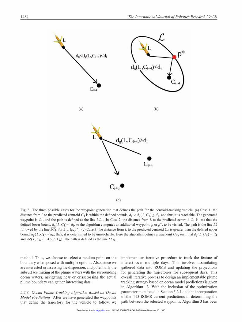
+ be the duration, in hours, of the planned mission. Theinput to the trajectory design algorithm is a set of points,D (referred to as drifters) that determine the initial extentof the plume (D0), and hourly predictions (Di, i ∈ T)of the location of each point in D. For the points in Di,we compute the convex hull as the minimum boundingellipsoid, Ei, for i ∈ T . We consider the predicted locationsof D0 after 4 h, D4. We let Ci be the centroid of Ei, and, witha slight abuse of notation, also refer to Ci as the centroidof Di. The algorithm computes dg( L, C4), where dg( x, y)is the geographical distance from x to y. Given upper andlower bounds du and dl, respectively, we have three possiblecases for choosing a location to send the glider to. Case 1:if dl < dg( L, C4) ≤ du, the generated waypoint is C4, andthe path is simply defined as the line LC4; see Figure 3(a).Case 2: if dg( L, C4) ≤ dl, the algorithm first checks to see ifthere exists a point p ∈ E4 ∪ D4 such that

dl ≤ dg( L, p) +dg( C4, p) ≤ du. (1)

If such a point exists, the algorithm generates two waypoints(p and C4) and the path is defined as the line Lp followedby the line pC4. In general, this will not be the case,since the distance from the centroid of the plume toits boundary can be many kilometers. Thus, if {p ∈E4 ∪ D4|dl ≤ dg( L, p) +dg( C4, p) ≤ du} = ∅, then thealgorithm computes the locus of points, L = {p∗ ∈L|dg(L, p) +dg( p, C4) = d4}, and selects a point at random,p∗ ∈ L, as another waypoint. Here the path is the line Lp∗followed by the line p∗C4; see Figure 3(b). This additionalwaypoint computation was inserted into the algorithm whenconsidering a single-vehicle deployment. In this scenario,one would like to acquire as much data as possible. Inthe case of a multiple-vehicle mission, it is less useful toinclude the additional waypoint in the trajectory design,as the other vehicles are gathering supplemental data.During deployment, p∗ is visited if and only if we feel thesafety of the vehicle will not be compromised by frequentsurfacings (e.g. based on geographical location, day of theweek and time of day). Case 3: if dg( L, C4) > du, thealgorithm generates a waypoint Cw in the direction of C6,such that dg( L, Cw) = d4; see Figure 3(c). The choice ofCi+6 over Ci+j, j ∈ {5, 7, 8}, is made here since Ci+6 isthe predicted location of the centroid halfway between the

surface interval times. Here we choose Ci+6 to be fixed forall scenarios, and, as in Smith et al. (2010c), we incorporateCi+j, j ∈ {5, 6, 7, 8}, as an optimization parameter to givethe glider the best chance of executing the prescribed path.Let AZ( a, b) be the azimuth angle between locations aand b. The location of the vehicle L is updated to C4 orCw and the process is iterated for the duration T . Thiswaypoint-generation process is presented in Algorithm 1.

Algorithm 1 Centroid-tracking, Waypoint-selectionAlgorithmRequire: Hourly forecasts, Di, for a set of points D

defining the initial plume condition and its movement fora period of time, T .for 0 ≤ i ≤ T do

Compute Ci, the centroid of the minimum boundingellipsoid Ei of the points Di. Compute d4.

end forwhile 0 ≤ i ≤ T − 1 do

if dl ≤ dg( L, Ci+4) ≤ du thenThe trajectory is LCi+4.

else if dg( L, Ci+4) ≤ dl and ∃p ∈ Ei+4 ∪Di+4 such thatdl ≤ dg( L, p) +dg( p, Ci+4) ≤ du then

The trajectory is Lp followed by pCi+4.else if dg( L, Ci+4) ≤ dl and {p ∈ Ei+4 ∪ Di+4|dl ≤dg( L, p) +dg( p, Ci+4) ≤ du} = ∅ then

Compute L = {p∗ ∈ L|dg( L, p) +dg( p, C4) = d4},select a random p∗ ∈ L and define the trajectory asLp∗ followed by p∗Ci+4.

else if dg( Ci, Ci+1) ≥ du thenCompute Cw such that dg( l, Cw) = d4 andAZ( L, Cw) = AZ( L, C6).

end ifend while

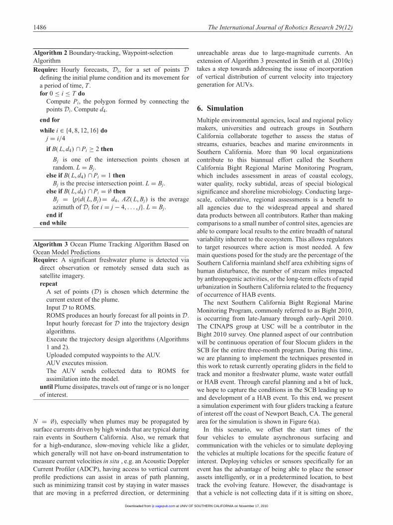
5.2.2. Boundary-tracking Algorithm Similarly to the pre-sentation in Section 5.2.1, we define the boundary-tracking,waypoint-generation algorithm, presented in Algorithm 2.We begin with the same predictions as above, and definePi to be the polygon formed by connecting the points Di

for i ∈ T . Let B( a, r) be the disc of radius r, about a.This algorithm first computes N = B( L, d4) ∩P4. Againwe have three possible cases to investigate to define thepath for the boundary-tracking vehicle. Case 1: if N ≥ 2,the generated waypoint B4 is a random selection of one ofthe intersection points; see Figure 4(a). Case 2: if N = 1,the generated waypoint B4 is that precise intersection point;see Figure 4(b). Case 3: if N = ∅, B4 is computed suchthat dg( L, B4) = d4 and AZ( L, B4) is the average azimuthof Di for the considered 4-h time period; see Figure 4(c).We reassign L = B4, and the algorithm is repeated. Forthe boundary-tracking scenario, it would be of interest totraverse the entire predicted extent of the given plume overthe duration of the survey. However, the test-bed vehiclesconsidered move too slowly to entertain this sampling




Fig. 3. The three possible cases for the waypoint generation that defines the path for the centroid-tracking vehicle. (a) Case 1: thedistance from L to the predicted centroid C4 is within the defined bounds, dl < dg( L, C4) ≤ du, and thus it is reachable. The generatedwaypoint is C4, and the path is defined as the line LC4. (b) Case 2: the distance from L to the predicted centroid C4 is less that thedefined lower bound, dg( L, C4) ≤ dl, so the algorithm computes an additional waypoint, p or p∗, to be visited. The path is the line Lkfollowed by the line kC4, for k ∈ {p, p∗}. (c) Case 3: the distance from L to the predicted centroid C4 is greater than the defined upperbound, dg( L, C4) > du; thus, it is determined to be unreachable. Here the algorithm defines a waypoint Cw, such that dg( L, Cw) = d4and AZ( L, Cw) = AZ( L, C6). The path is defined as the line LCw.

method. Thus, we choose to select a random point on theboundary when posed with multiple options. Also, since weare interested in assessing the dispersion, and potentially thesubsurface mixing of the plume waters with the surroundingocean waters, navigating near or crisscrossing the actualplume boundary can gather interesting data.

5.2.3. Ocean Plume Tracking Algorithm Based on OceanModel Predictions After we have generated the waypointsthat define the trajectory for the vehicle to follow, we

implement an iterative procedure to track the feature ofinterest over multiple days. This involves assimilatinggathered data into ROMS and updating the projectionsfor generating the trajectories for subsequent days. Thisoverall iterative process to design an implementable plumetracking strategy based on ocean model predictions is givenin Algorithm 3. With the inclusion of the optimizationparameter mentioned in Section 5.2.1 and the incorporationof the 4-D ROMS current predictions in determining thepath between the selected waypoints, Algorithm 3 has been



Smith et al. 1485

Fig. 4. The three possible cases for the waypoint generation that defines the path for the boundary-tracking vehicle. (a) Case 1: a circleof radius d4 about L intersects the predicted polygon that defines the boundary of the plume, P4, at least twice, N ≥ 2. The generatedwaypoint B4 is a random selection of one of these intersection points, and the path is defined as LB4. (b) Case 2: a circle of radius d4about L intersects the predicted polygon that defines the boundary of the plume, P4, exactly once, N = 1. The generated waypoint B4 isthe intersection point, and the path is defined as LB4. (c) Case 3: a circle of radius d4 about L does not intersect the predicted polygonthat defines the boundary of the plume, P4, N = ∅. The generated waypoint B4 is computed such that dg( L, B4) = d4 and AZ( L, B4) isthe average azimuth of Di for the considered 4-h time period, and the path is defined as LB4.

extended in Smith et al. (2010c), and is renamed the oceanplume tracking algorithm built on ocean model predictions(OPTA-BLOOM-Pred).

In the following sections, we proceed to presentsimulation and field experiments that implement pathsgenerated by use of Algorithm 3. By construction, thesepaths are generated to track a plume that propagates onthe ocean surface (0–30 m), while the vehicle used totrack them, i.e. a Slocum glider, operates from the surfacedown to depths of ∼ 80 m. It is not valid to assume that

both of these are subjected to the same current regime,in both velocity and direction. In particular, a verticalvelocity profile of ocean current for a given location withinthe SCB is, in general, not constant. This observation isillustrated in Figure 5 with an example plot of currentvelocity versus depth. Figure 5 displays a ROMS predictionfor the meridional component of a vertical current profilelocated at 33.58◦ N, −118.38◦ E for 8 July 2009. Fromthis example, we see that it may be possible for a plumeto outrun a slow-moving vehicle (i.e. dg( Ci, Ci+1) ≥ du or




Algorithm 2 Boundary-tracking, Waypoint-selectionAlgorithmRequire: Hourly forecasts, Di, for a set of points D

defining the initial plume condition and its movement fora period of time, T .for 0 ≤ i ≤ T do

Compute Pi, the polygon formed by connecting thepoints Di. Compute d4.

end for

while i ∈ {4, 8, 12, 16} doj = i/4

if B( L, d4) ∩ Pi ≥ 2 then

Bj is one of the intersection points chosen atrandom. L = Bj.

else if B( L, d4) ∩ Pi = 1 thenBj is the precise intersection point. L = Bj.

else if B( L, d4) ∩ Pi = ∅ thenBj = {p|d( L, Bj) = d4, AZ( L, Bj) is the averageazimuth of Di for i = j − 4, . . . , j}. L = Bj.

end ifend while

Algorithm 3 Ocean Plume Tracking Algorithm Based onOcean Model PredictionsRequire: A significant freshwater plume is detected via

direct observation or remotely sensed data such assatellite imagery.repeat

A set of points (D) is chosen which determine thecurrent extent of the plume.Input D to ROMS.ROMS produces an hourly forecast for all points in D.Input hourly forecast for D into the trajectory designalgorithms.Execute the trajectory design algorithms (Algorithms1 and 2).Uploaded computed waypoints to the AUV.AUV executes mission.The AUV sends collected data to ROMS forassimilation into the model.

until Plume dissipates, travels out of range or is no longerof interest.

N = ∅), especially when plumes may be propagated bysurface currents driven by high winds that are typical duringrain events in Southern California. Also, we remark thatfor a high-endurance, slow-moving vehicle like a glider,which generally will not have on-board instrumentation tomeasure current velocities in situ , e.g. an Acoustic DopplerCurrent Profiler (ADCP), having access to vertical currentprofile predictions can assist in areas of path planning,such as minimizing transit cost by staying in water massesthat are moving in a preferred direction, or determining

unreachable areas due to large-magnitude currents. Anextension of Algorithm 3 presented in Smith et al. (2010c)takes a step towards addressing the issue of incorporationof vertical distribution of current velocity into trajectorygeneration for AUVs.

6. Simulation

Multiple environmental agencies, local and regional policymakers, universities and outreach groups in SouthernCalifornia collaborate together to assess the status ofstreams, estuaries, beaches and marine environments inSouthern California. More than 90 local organizationscontribute to this biannual effort called the SouthernCalifornia Bight Regional Marine Monitoring Program,which includes assessment in areas of coastal ecology,water quality, rocky subtidal, areas of special biologicalsignificance and shoreline microbiology. Conducting large-scale, collaborative, regional assessments is a benefit toall agencies due to the widespread appeal and shareddata products between all contributors. Rather than makingcomparisons to a small number of control sites, agencies areable to compare local results to the entire breadth of naturalvariability inherent to the ecosystem. This allows regulatorsto target resources where action is most needed. A fewmain questions posed for the study are the percentage of theSouthern California mainland shelf area exhibiting signs ofhuman disturbance, the number of stream miles impactedby anthropogenic activities, or the long-term effects of rapidurbanization in Southern California related to the frequencyof occurrence of HAB events.

The next Southern California Bight Regional MarineMonitoring Program, commonly referred to as Bight 2010,is occurring from late-January through early-April 2010.The CINAPS group at USC will be a contributor in theBight 2010 survey. One planned aspect of our contributionwill be continuous operation of four Slocum gliders in theSCB for the entire three-month program. During this time,we are planning to implement the techniques presented inthis work to retask currently operating gliders in the field totrack and monitor a freshwater plume, waste water outfallor HAB event. Through careful planning and a bit of luck,we hope to capture the conditions in the SCB leading up toand development of a HAB event. To this end, we presenta simulation experiment with four gliders tracking a featureof interest off the coast of Newport Beach, CA. The generalarea for the simulation is shown in Figure 6(a).

In this scenario, we offset the start times of thefour vehicles to emulate asynchronous surfacing andcommunication with the vehicles or to simulate deployingthe vehicles at multiple locations for the specific feature ofinterest. Deploying vehicles or sensors specifically for anevent has the advantage of being able to place the sensorassets intelligently, or in a predetermined location, to besttrack the evolving feature. However, the disadvantage isthat a vehicle is not collecting data if it is sitting on shore,



Smith et al. 1487

Fig. 5. An example vertical current profile prediction for a location within the SCB. This is a ROMS prediction of ocean depth versuscurrent velocity for the meridional component located at 33.58◦ N, −118.38◦ E. This is a prediction made for 8 July 2009.

and important aspects of algal bloom development andevolution may be missed. Additionally, events occurring onshorter time scales may be entirely missed, as deploymentsdo not always go as planned. For the features of interestconsidered in this study, even intelligent deployment can benon-trivial. As an example, consider the difference betweena freshwater river runoff plume and a subsurface effluentalgal bloom. Freshwater river outfall plumes are buoyant,and float high in the water. In general, these plumes havea stronger leading edge, i.e. sharper gradient, and a morediluted trailing edge. Thus, deploying gliders at the frontof the plume may provide more information and allow thevehicle a better chance to remain in contact with the feature.For an algal bloom, it is a bit more complicated, as theboundary of the bloom is dependent on the kind of systemthat it is embedded in. In particular, subsurface effluentplumes are submerged, and become density equilibrated,making the boundary of the bloom more difficult to discern.Also, contrary to a freshwater plume, an algal bloom iscomposed of living organisms, whose life-cycle dynamicsaffect the movement and structure of the bloom in additionto the ocean currents. These chemical and biologicaldynamics, along with the 3-D composition and evolution ofan algal bloom, are poorly understood, and are a primarymotivation for developing techniques to place mobilesensors in the right place at the right time to gather data thatwill increase our understanding of these complex systems.

For the simulation, at T = 0 h, we deploy two vehicles,one centroid tracker and one boundary tracker, at thesouthern extent of the plume (predicted plume front). AtT = 2 h we deploy a boundary-tracking vehicle onthe predicted western boundary of the plume. Finally, atT = 4h, we start a boundary-tracking vehicle at thepredicted northern boundary of the plume (predictedtrailing edge of the plume). The initial delineation andlocation of the first two gliders are presented in Figure 6(a).The evolution of the plume with vehicle trajectories ispresented in Figures 6(a)–7(f). The trajectories of thevehicles are the expected trajectories of the gliders,projected to the ocean surface. Note that in Figures 6(a)–7(f), we only display a trajectory for a vehicle at thehour when it surfaces due to the offset in start times. Thepredicted extent of the plume is delineated by the closedpolygon. The centroid of the predicted plume is depictedby the dot inside the delineated plume extent; the centroid-tracking vehicle follows the path given by the solid line andthe boundary-tracking vehicles follow the paths given bythe dashed lines.

The trajectory design is based upon model predictions,and we are familiar with the deployment area; we do have ana priori understanding of the general direction the featureshould travel in. This knowledge can be used to select theinitial locations of the vehicles based upon the informationto be gathered and areas of interest within the feature. In this




Fig. 6. Simulation results for four vehicles tracking a propagating plume. The plume extent is delineated by the closed polygon. Threevehicles (dashed line paths) follow the boundary, while one vehicle (solid line path) tracks the centroid of the plume. The centroid isdepicted by the dot inside the delineated plume extent. Panel (a) provides the initial delineation of the plume in the coastal region nearLos Angeles, CA. Panel (b) presents an enlarged image of panel (a). Panels (b)–(f) present snapshots every 2 h of the tracking simulationfrom initialization to T = 8 h. The scale given in panel (b) is the same for panels (c)–(f). Images created by use of Google Earth.

example, since we see a rather fast-moving feature in thesoutheast direction, we choose to start the centroid trackeron the southern extent, or leading edge, of the feature.Thus, we do not try and chase the area we are interestedin sampling, and have a higher probability of collectingdata within the plume. Based on the movement of thefeature, the centroid-tracking vehicle (solid line) actuallycompletes a U-shape trajectory, and from T = 12 to 16hcannot keep up with the feature, based on our constant-speed assumption. We also see the speed of the feature since

the boundary-tracking vehicles (dashed lines) traverse moreof a straight-line path than the zig-zag seen with a slower-moving feature as in Figures 11(f) and 12(e). Overall, thetrajectories presented here, and in the previous deploymentsections, do not resemble those that a human operator woulddesign. However, the trajectories do guide the vehiclesthrough a large portion of the plume during its predictedevolution, thus increasing the probability of collecting high-valued data for both the marine biology community and themodeling community alike.



Smith et al. 1489

Fig. 7. Continuation of the simulation results for four vehicles tracking a propagating plume presented in Figure 6. The plume extent isdelineated by the closed polygon. Three vehicles (dashed line paths) follow the boundary, while one vehicle (solid line path) tracks thecentroid of the plume. The centroid is depicted by the dot inside the delineated plume extent. Panels (a)–(f) present snapshots every twohours of the tracking simulation from T = 10 h to completion (T = 20 h). The scale for all images is given in panel (a). Images createdby use of Google Earth.

7. Implementation and Field Experiments inthe SCB

We present the results of two field deployments, duringwhich we implemented trajectories designed by Algorithm3. In Section 7.1 we present the results of a single-vehicle, centroid-tracking mission initially presented inSmith et al. (2009a). We follow this in Section 7.2 witha two-vehicle mission, tracking both the centroid and theboundary of a plume. We remark to the reader that the

implementation of the path plans generated here wouldideally be implemented and executed in an opportunisticfashion onto a currently deployed vehicle. In this case,the ability to select the initial location of the vehiclewith respect to the feature of interest is not practical. Inthe following field trials, the vehicles were on a routinedeployment and the presented experiments are meant tosimulate an opportunistic retasking event. Note that theplume we wish to track is delineated close to near-future




surfacing locations of the gliders so that missions canbe uploaded and executed in a timely fashion, and thevehicles can continue with the previous routine survey.Initial locations of the vehicles with respect to the plumedelineation are purposefully chosen to be suboptimalto present a real-life situation. An alternate scenario toopportunistic retasking is to consider that the vehicles aredeployed specifically for a detected algal bloom or riverplume. This situation has been addressed in the simulationexperiment presented in Section 6.

As noted in Smith et al. (2009a), the rainy season inSouthern California is generally between November andMarch. During this time, storm events cause large runoffinto local-area rivers and streams, all of which empty intothe Pacific Ocean. Two major rivers in the Los Angelesarea, the Santa Ana and the Los Angeles River, inputlarge freshwater plumes to the SCB. Such plumes have ahigh likelihood of producing HABs. Unfortunately, duringboth deployments, weather and/or remote-sensing devicesdid not cooperate to produce a rain event along witha detectable plume. For both cases presented here, wedefined a pseudo-plume in two separate areas of the SCBto demonstrate a proof-of-concept of the technology chainand trajectory design method developed here.

For the centroid-tracking mission, we deployed a gliderinto the SCB on 17 February 2009 to conduct a month-longobservation and sampling mission. For this deployment, theglider was programmed to execute a zig-zag pattern missionalong the coastline, as depicted in Figure 8, by navigatingto each of the six waypoints depicted by the bullseyes.During execution of this mission, we retasked the glidermid-mission and uploaded the centroid-tracking trajectorydescribed in Section 7.1.

For the boundary-tracking mission, we deployed twogliders off the northeast tip of Santa Catalina Island on29 April 2009 to conduct a month-long experiment totest the communication infrastructure described in Smithet al. (2010a). For this mission, there was not a single,predetermined path for the glider to traverse as before, butwe had the ability to retask the vehicles as needed. Thedetails of this mission, with regard to the communicationdata collected, can be found in Pereira et al. (2009) andSmith et al. (2009b). The 2-day mission presented belowwas conducted during 11–13 May 2009.

7.1. Centroid Tracking

The mission presented in this section is reproduced fromSmith et al. (2009a). Since Algorithm 1 has been modifiedbased on the lessons learned during the execution ofthis deployment, there are slight discrepancies in planningbetween the following description and the method presentedin Algorithm 1. However, the general idea and methodologyis the same.

For this mission, we defined a pseudo-plume D with 15initial drifter locations off the coast of Newport Beach, CA.The pseudo-plume is given by the dashed line in Figure 9.

Fig. 8. The intended glider path of the month-long, zig-zagpattern mission started on 17 February 2009 is given by the solidline. The preset waypoints that define this path and were uploadedto the glider are depicted by the bullseyes. This path represents aroutine deployment mission carried out regularly by USC CINAPSgliders. Image created by use of Google Earth.

Fig. 9. An overview of the delineated plume to track and thecomputed path to track the centroid of the plume. The solidline connecting bullseyes represents the routine zig-zag missionpresented in Figure 8. The initial delineation of the plume to trackis given by the dashed line. The waypoints generated by Algorithm1 are represented by the numbered diamonds. The intended gliderpath (projected to the ocean surface) is the solid line connectingthe consecutively numbered waypoints. Image created by use ofGoogle Earth.

By use of ROMS, the locations of the points in D werepredicted for T = 15 h. The initial time and location forthe beginning of this retasking experiment coincided withpredicted coordinates of a future glider communication.The pseudo-plume was chosen such that C0 was near thispredicted glider surfacing location.

Based on observed behavior for our vehicle during thisdeployment, we take v = 0.75 km h−1, and initially defined



Smith et al. 1491

Table 1. A Complete Listing of the Waypoints Generated by Algorithm 1. Waypoint Numbers 1, 3, 5 and 7 are the Predicted Centroidsof the Pseudo-plume at Hours 0, 5, 10 and 15, Respectively. Waypoint Numbers 2, 4 and 6 are the Additional Locations (p∗ ∈ L) to beVisited as Computed in Case 2 (dg( L, C4) ≤ dl) of Algorithm 1

Number Latitude (◦ N) Longitude (◦ E) Number Latitude (◦ N) Longitude (◦ E)

1 33.6062 –118.0137 5 33.6189 –118.03492 33.6054 –118.0356 6 33.6321 –118.02573 33.6180 –118.0306 7 33.6175 –118.03614 33.6092 –118.0487

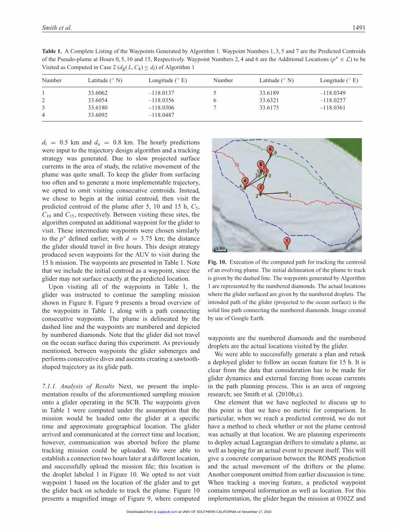
dl = 0.5 km and du = 0.8 km. The hourly predictionswere input to the trajectory design algorithm and a trackingstrategy was generated. Due to slow projected surfacecurrents in the area of study, the relative movement of theplume was quite small. To keep the glider from surfacingtoo often and to generate a more implementable trajectory,we opted to omit visiting consecutive centroids. Instead,we chose to begin at the initial centroid, then visit thepredicted centroid of the plume after 5, 10 and 15 h, C5,C10 and C15, respectively. Between visiting these sites, thealgorithm computed an additional waypoint for the glider tovisit. These intermediate waypoints were chosen similarlyto the p∗ defined earlier, with d = 3.75 km; the distancethe glider should travel in five hours. This design strategyproduced seven waypoints for the AUV to visit during the15 h mission. The waypoints are presented in Table 1. Notethat we include the initial centroid as a waypoint, since theglider may not surface exactly at the predicted location.

Upon visiting all of the waypoints in Table 1, theglider was instructed to continue the sampling missionshown in Figure 8. Figure 9 presents a broad overview ofthe waypoints in Table 1, along with a path connectingconsecutive waypoints. The plume is delineated by thedashed line and the waypoints are numbered and depictedby numbered diamonds. Note that the glider did not travelon the ocean surface during this experiment. As previouslymentioned, between waypoints the glider submerges andperforms consecutive dives and ascents creating a sawtooth-shaped trajectory as its glide path.

7.1.1. Analysis of Results Next, we present the imple-mentation results of the aforementioned sampling missiononto a glider operating in the SCB. The waypoints givenin Table 1 were computed under the assumption that themission would be loaded onto the glider at a specifictime and approximate geographical location. The gliderarrived and communicated at the correct time and location;however, communication was aborted before the plumetracking mission could be uploaded. We were able toestablish a connection two hours later at a different location,and successfully upload the mission file; this location isthe droplet labeled 1 in Figure 10. We opted to not visitwaypoint 1 based on the location of the glider and to getthe glider back on schedule to track the plume. Figure 10presents a magnified image of Figure 9, where computed

Fig. 10. Execution of the computed path for tracking the centroidof an evolving plume. The initial delineation of the plume to trackis given by the dashed line. The waypoints generated by Algorithm1 are represented by the numbered diamonds. The actual locationswhere the glider surfaced are given by the numbered droplets. Theintended path of the glider (projected to the ocean surface) is thesolid line path connecting the numbered diamonds. Image createdby use of Google Earth.

waypoints are the numbered diamonds and the numbereddroplets are the actual locations visited by the glider.

We were able to successfully generate a plan and retaska deployed glider to follow an ocean feature for 15 h. It isclear from the data that consideration has to be made forglider dynamics and external forcing from ocean currentsin the path planning process. This is an area of ongoingresearch; see Smith et al. (2010b,c).

One element that we have neglected to discuss up tothis point is that we have no metric for comparison. Inparticular, when we reach a predicted centroid, we do nothave a method to check whether or not the plume centroidwas actually at that location. We are planning experimentsto deploy actual Lagrangian drifters to simulate a plume, aswell as hoping for an actual event to present itself. This willgive a concrete comparison between the ROMS predictionand the actual movement of the drifters or the plume.Another component omitted from earlier discussion is time.When tracking a moving feature, a predicted waypointcontains temporal information as well as location. For thisimplementation, the glider began the mission at 0302Z and




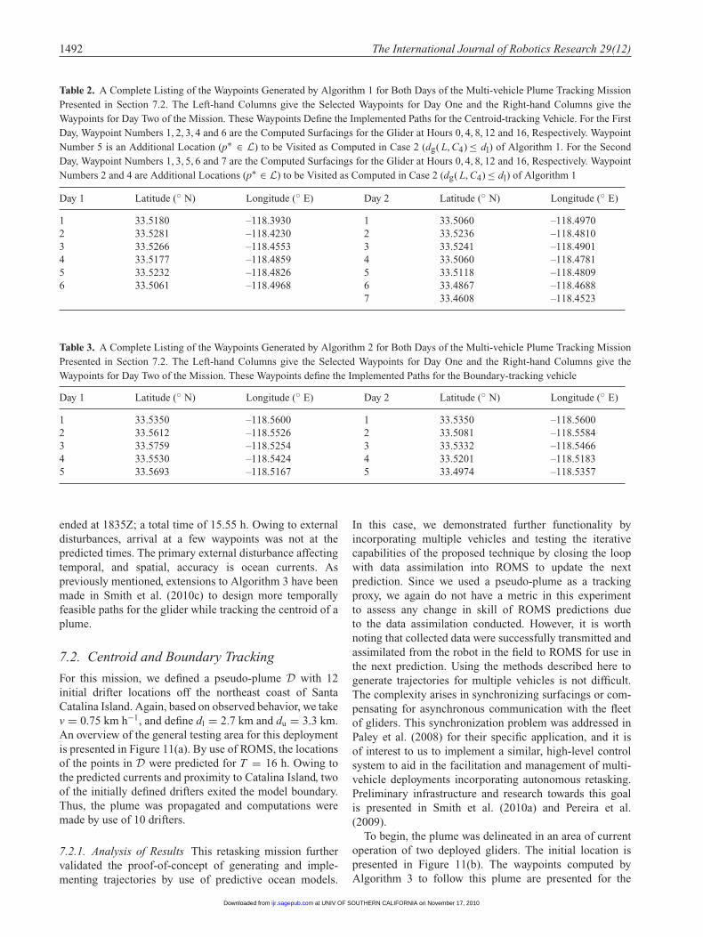
Table 2. A Complete Listing of the Waypoints Generated by Algorithm 1 for Both Days of the Multi-vehicle Plume Tracking MissionPresented in Section 7.2. The Left-hand Columns give the Selected Waypoints for Day One and the Right-hand Columns give theWaypoints for Day Two of the Mission. These Waypoints Define the Implemented Paths for the Centroid-tracking Vehicle. For the FirstDay, Waypoint Numbers 1, 2, 3, 4 and 6 are the Computed Surfacings for the Glider at Hours 0, 4, 8, 12 and 16, Respectively. WaypointNumber 5 is an Additional Location (p∗ ∈ L) to be Visited as Computed in Case 2 (dg( L, C4) ≤ dl) of Algorithm 1. For the SecondDay, Waypoint Numbers 1, 3, 5, 6 and 7 are the Computed Surfacings for the Glider at Hours 0, 4, 8, 12 and 16, Respectively. WaypointNumbers 2 and 4 are Additional Locations (p∗ ∈ L) to be Visited as Computed in Case 2 (dg( L, C4) ≤ dl) of Algorithm 1

Day 1 Latitude (◦ N) Longitude (◦ E) Day 2 Latitude (◦ N) Longitude (◦ E)

1 33.5180 –118.3930 1 33.5060 –118.49702 33.5281 –118.4230 2 33.5236 –118.48103 33.5266 –118.4553 3 33.5241 –118.49014 33.5177 –118.4859 4 33.5060 –118.47815 33.5232 –118.4826 5 33.5118 –118.48096 33.5061 –118.4968 6 33.4867 –118.4688

7 33.4608 –118.4523

Table 3. A Complete Listing of the Waypoints Generated by Algorithm 2 for Both Days of the Multi-vehicle Plume Tracking MissionPresented in Section 7.2. The Left-hand Columns give the Selected Waypoints for Day One and the Right-hand Columns give theWaypoints for Day Two of the Mission. These Waypoints define the Implemented Paths for the Boundary-tracking vehicle

Day 1 Latitude (◦ N) Longitude (◦ E) Day 2 Latitude (◦ N) Longitude (◦ E)

1 33.5350 –118.5600 1 33.5350 –118.56002 33.5612 –118.5526 2 33.5081 –118.55843 33.5759 –118.5254 3 33.5332 –118.54664 33.5530 –118.5424 4 33.5201 –118.51835 33.5693 –118.5167 5 33.4974 –118.5357

ended at 1835Z; a total time of 15.55 h. Owing to externaldisturbances, arrival at a few waypoints was not at thepredicted times. The primary external disturbance affectingtemporal, and spatial, accuracy is ocean currents. Aspreviously mentioned, extensions to Algorithm 3 have beenmade in Smith et al. (2010c) to design more temporallyfeasible paths for the glider while tracking the centroid of aplume.

7.2. Centroid and Boundary Tracking

For this mission, we defined a pseudo-plume D with 12initial drifter locations off the northeast coast of SantaCatalina Island. Again, based on observed behavior, we takev = 0.75 km h−1, and define dl = 2.7 km and du = 3.3 km.An overview of the general testing area for this deploymentis presented in Figure 11(a). By use of ROMS, the locationsof the points in D were predicted for T = 16 h. Owing tothe predicted currents and proximity to Catalina Island, twoof the initially defined drifters exited the model boundary.Thus, the plume was propagated and computations weremade by use of 10 drifters.

7.2.1. Analysis of Results This retasking mission furthervalidated the proof-of-concept of generating and imple-menting trajectories by use of predictive ocean models.

In this case, we demonstrated further functionality byincorporating multiple vehicles and testing the iterativecapabilities of the proposed technique by closing the loopwith data assimilation into ROMS to update the nextprediction. Since we used a pseudo-plume as a trackingproxy, we again do not have a metric in this experimentto assess any change in skill of ROMS predictions dueto the data assimilation conducted. However, it is worthnoting that collected data were successfully transmitted andassimilated from the robot in the field to ROMS for use inthe next prediction. Using the methods described here togenerate trajectories for multiple vehicles is not difficult.The complexity arises in synchronizing surfacings or com-pensating for asynchronous communication with the fleetof gliders. This synchronization problem was addressed inPaley et al. (2008) for their specific application, and it isof interest to us to implement a similar, high-level controlsystem to aid in the facilitation and management of multi-vehicle deployments incorporating autonomous retasking.Preliminary infrastructure and research towards this goalis presented in Smith et al. (2010a) and Pereira et al.(2009).

To begin, the plume was delineated in an area of currentoperation of two deployed gliders. The initial location ispresented in Figure 11(b). The waypoints computed byAlgorithm 3 to follow this plume are presented for the



Smith et al. 1493

Fig. 11. Deployment results for the first day of the mission for two vehicles to track an evolving plume. The plume extent is delineatedby the closed polygon. One vehicle (dashed line path) follows the boundary, while one vehicle (solid line path) tracks the centroid of theplume. The centroid is depicted by the dot inside the delineated plume extent. Panel (a) provides an overview of the deployment area offthe coast of Los Angeles, CA. Panel (b) presents an enlarged image of the deployment area just off the northeast coast of Santa CatalinaIsland, CA with the initial delineation of the plume. Panels (b)–(f) present snapshots every four hours of the tracking experiment frominitialization to completion (T = 16 h) for the first day. The scale given in panel (b) is the same for panels (c)–(f). Images created byuse of Google Earth.

centroid- and boundary-tracking vehicles in the left-handcolumns of Tables 2 and 3, respectively. The initial timeand location for the beginning of this retasking experimentcoincided with predicted coordinates of glider surfacings.Since the assigned mission was to collect communicationdata, the vehicles were surfacing frequently (� 2 hintervals). This made coordinating surfacing time much

more manageable than in the scenario presented in Section7.1, where the glider was surfacing approximately every8 h. In addition, communication via our implementedFreewave™ network (Pereira et al. 2009) facilitated morerobust communication, as well as more rapid file exchangethan during previous deployments. Once both gliders wereon the surface together (approximately 1800Z, 11 May




2009), we ran Algorithm 3 with the location of each gliderinitially being on the boundary of the plume. Figure 11(b)(f)display the delineation of the plume with the locations ofboth gliders at 4-h increments from T = 0 h (Figure 11(b))to T = 16 h (Figure 11(f)). In these figures, the boundary-tracking glider follows the dashed line and the centroid-tracking glider follows the solid line. The respective iconsalong the paths denote the locations where the glidersurfaced while executing the mission. When visible, thedot inside the polygonal delineation of the plume extentrepresents the predicted centroid of the plume; when notseen, the centroid-tracking glider surfaced within 500 m ofthe location of the predicted centroid. The solid and dashedlines depict the path of the glider (projected to the surface)between surfacings. Note that in the initial four hours of themission, the plume moved northward, and the boundary-tracking vehicle was on the leading edge. However, afterthe initial few hours, the plume migrated southward and theboundary-tracking glider ended up following the trailingedge of the plume. Day one of this mission ended shortlyafter 1000Z on 12 May 2009.

Upon completion of the day-one mission, the glidersresumed their previous missions of gathering communica-tion data while we awaited the following day’s ROMS pre-diction. The entire process mentioned above was repeatedbeginning at approximately 2200Z on 12 May 2009. Theinitial plume delineation, glider surfacing locations andprojected trajectories are given in Figure 12(a-e). The com-puted waypoints for the centroid- and boundary-trackingvehicles are given in the right-hand columns of Tables2 and 3, respectively. Day two of the mission completedshortly after 1400Z on 13 May 2009. Note that at thestart of day two, we redelineated the plume differentlyfrom the final predicted configuration of day one. This isapplicable in practice because we cannot assume ROMSto be 100% accurate, and we have a time gap betweenthe start of the sampling missions where we expect theplume to further evolve. Additionally, we are forecastingthe evolution of a plume based on the predicted paths ofmultiple, unconnected, Lagrangian drifters, which may notbehave exactly like a contiguous ocean feature.

Overall, this 2-day mission validated both the multi-vehicle applicability as well as the ability to close the loopon the technology toolchain from ROMS to path planningto field AUV and back to ROMS. This further motivatesour efforts to prepare for a large-scale deployment, such asBight 2010 presented in Section 6, with hopes of locatingand tracking a plume from a significant rain event runoff, ora HAB.

8. Conclusions and Future Work

In the study of path planning for field robots, designingthe trajectory is usually less than half the battle; the realchallenge comes in the implementation. This is exaggeratedwhen dealing with underwater robots due to the complex,

and often unknown, environment. Poorly understood oceandynamics, difficulty in localization and extreme conditionsall contribute to the struggle of successful implementationof a planned mission for an AUV. In this paper, we examinedthe use of ocean model predictions to help reduce some ofthis uncertainty for the application of path planning to trackan evolving ocean feature.

Generating effective sampling strategies to study oceanphenomena is a challenging task that can be approachedfrom many different angles. Here we presented a method toexploit multiple facets of technology to achieve our goal.Utilizing an ocean model, an embedded sensor networkand an AUV, we were able to construct a technology chainwhich plans a path to track areas of scientific interestwithin a chosen feature of interest for a chosen period oftime. This toolchain was used to design a single-vehiclemission to track a plume’s centroid, and generate the pathsfor a multi-vehicle mission for simultaneous sampling atthe centroid as well as along the boundary of a givenfeature. We presented iterated field trials to demonstrateclosing the loop of the technology chain developed aswell as to demonstrate a proof-of-concept of the planningmethod presented. This paper has demonstrated that wehave implemented the collaboration and technology chainrequired to perform complex field experiments to trackdynamically evolving ocean features. Research is ongoingto extend and improve upon the presented waypoint-generation and path planning algorithms to incorporateROMS 4-D velocity predictions to improve the accuracyof the implementation (Smith et al. 2010c). Additionally,we are interested in assessing the accuracy of ROMSvelocity predictions, and the performance and reliabilityof our gliders to more effectively utilize them to furtherour understanding of the life cycle of an algal bloom(Smith et al. 2010b). We remark that the implementationand realization of the paths generated in this paperwere perfectly feasible, given that there was no temporalconstraint. Improving the temporal feasibility along withthe spatial accuracy is a primary focus of ongoingand future work in this area. Based on the operationalconstraints of the gliders, these are not the optimalvehicles to chase fast-moving events or adaptively react todynamically changing conditions. The CINAPS team is inthe process of acquiring a different type of AUV that ismore agile and can more effectively carry out the strategiesdesigned here, with specific regard to fast-moving features.

The main implementation issue is the assumed ability ofthe glider to accurately navigate to a given waypoint. Ingeneral, this is a widely studied, and currently unsolved,problem in underwater robotics. For the results presentedhere, this artifact is a result of the waypoint-selectionalgorithms only utilizing a 2-D propagation of the plume,and ignoring the dynamics of the glider and predictedvertical velocity profiles when generating the final pathplan. Research is active to extend these results toincorporate the kinematic and dynamic aspects of the



Smith et al. 1495

Fig. 12. Deployment results for the second day of the mission for two vehicles to track an evolving plume. The plume extent isdelineated by the closed polygon. One vehicle (dashed line path) follows the boundary, while one vehicle (solid line path) tracks thecentroid of the plume. The centroid is depicted by the dot inside the delineated plume extent. Panel (a) presents an enlarged image ofthe deployment area just off the northeast coast of Santa Catalina Island, CA with an updated delineation of the plume for the start ofday two. Panels (a)–(e) present snapshots every four hours of the tracking experiment from initialization to completion (T = 16 h) forthe second day. The scale given in panel (a) is the same for panels (b)–(e). Images created by use of Google Earth.

glider, see Smith et al. (2010b), and extend this methodof path planning from a planar to a 3-D path planningalgorithm and trajectory generation toolchain, see Smithet al. (2010c). As mentioned previously, we are makingprogress to increase the performance of the AUV throughthe use of ocean model predictions, but at this time weare still not equipped to utilize ROMS predictions topropagate a feature of interest in 4-D. The primary reason

for this is based on the lack of understanding and detectioncapabilities of the initial 3-D structure and extent of agiven plume. Algal blooms, in particular, are too poorlyunderstood to hypothesize about their 3-D spatial extent; wecurrently have difficulties determining and predicting their2-D extent.

A long-term goal of this effort is to utilize the embeddedsensor network presented in Smith et al. (2010a) and




Pereira et al. (2009) to enable real-time, optimal trajectorydesign, based on ocean model predictions, to gatherin situ measurements of interesting and evolving oceanfeatures and phenomena while additionally increasing theskill of regional ocean models. Through this effort, we aimto quantitatively assess the effectiveness of ocean modelpredictions in the design and accurate implementation oftrajectories for AUVs. As previously mentioned, this willcome with deployment of actual drifters simulating thepropagation of a feature, or the occurrence of an actualHAB event during Bight 2010.

As discussed in Section 6, a more immediate implemen-tation of the methods developed here will be used duringour participation in Bight 2010. Currently, we are expe-riencing weak El Niño conditions, as equatorial Pacific,sea-surface temperatures remained above average throughAugust 2009. These conditions are expected to strengthenthrough winter 2009–2010 in the Northern Hemisphere(Climate Prediction Center 2009), and have impactedSouthern California with more frequent and intense stormevents in early 2010. From the discussion in Sections 2.1and 2.2, we can infer that the potential for the formation ofconditions that may promote an algal bloom is increasedover the next year. Such information presents a greateropportunity to retest and validate our methods and algo-rithms in a real scenario. Thus, we are motivated to furtherdevelop our algorithms to steer AUVs into locations ofhigh scientific merit with regard to HAB research and helpocean scientists better understand these complex phenom-ena, while additionally assessing the prediction capabilitiesof regional ocean models.

Acknowledgements

This work was supported in part by the NOAA MERHABprogram under grant NA05NOS4781228 and by NSF aspart of the Center for Embedded Network Sensing (CENS)under grant CCR-0120778, by NSF grants CNS-0520305and CNS-0540420, by the ONR MURI program (grantsN00014-09-1-1031 and N00014-08-1-0693), by the ONRSoA program and by a gift from the Okawa Foundation.The ROMS ocean modeling research described in this paperwas carried out by the Jet Propulsion Laboratory (JPL),California Institute of Technology, under a contract with theNational Aeronautics and Space Administration (NASA).

The authors acknowledge Carl Oberg for his work withglider hardware making field implementations possible andsimple. We thank Ivona Cetinic, Arvind Pereira and HördurHeidarsson for their efforts in the glider deployment andcommunications during the missions.

Notes

1. The SCB is the oceanic region contained within 32◦ N to34.5◦ N and −117◦ E to −121◦ E.

2. The SCB is a very high traffic region, and the glider has a lowvisual profile when on the surface. Although the probabilityof a collision is low, we choose to err on the side of caution.

References

Anderson, D. (2008). Harmful algae, http://www.whoi.edu/redtide/page.do?pid=9257 (accessed February 2009).

Cetinic, I., Jones, B. H., Moline, M. A. and Schofield, O. (2010).Resolving urban plumes using autonomous gliders in thecoastal ocean, Continental Shelf Research.

Chao, Y., Li, Z., Farrara, J., McWilliams, J. C., Bellingham, J.,Capet, X., et al. (2008). Development, implementation andevaluation of a data-assimilative ocean forecasting systemoff the central California coast, Deep-Sea Research II, 56:100–126.

Climate Prediction Center (2009). El Niño/Southern Oscillation(ENSO) diagnostic discussion, http://www.cpc.noaa.gov/products/analysis_monitoring/enso_advisory/ensodisc.html(accessed September 2009).

Dailey, M. D., Reish, D. J. and Anderson, J. W. (eds.) (1993).Ecology of the Southern California Bight. Berkeley, CA,University of California Press.

Das, J., Rajan, K., Frolov, S., Ryan, J., Py, F., Caron, D. A.and Sukhatme, G. S. (2010). Towards marine bloomtrajectory prediction for AUV mission planning. IEEEInternational Conference on Robotics and Automation, http://cres.usc.edu/cgi-bin/print_pub_details.pl?pubid=637.

Davis, R. E., Ohman, M., Rudnick, D., Sherman, J. and Hodges,B. (2008). Glider surveillance of physics and biology in theSouthern California current system. Limnology Oceanography,53: 2151–2168.

Fiorelli, E., Leonard, N., Bhatta, P., Paley, D., Bachmayer, R.and Fratantoni, D. (2006). Multi-AUV control and adaptivesampling in Monterey Bay, IEEE Journal of OceanicEngineering, 31(4): 935–948.

Graver, J. G. (2005). Underwater Gliders: Dynamics, Control andDesign. PhD Thesis, Princeton University.

Gray, A. M., Lee, C., D’Asaro, E. A., Perry, M. J., Fennel,K., Briggs, N., Rehm, E., Sackmann, B. S., Sieracki, M. E.,Poulton, N. and Gudmundsson, K. (2008), The 2008 northatlantic spring bloom experiment: observations of a stationaryeddy on the eastern flank of the Reykjanes Ridge. AmericanGeophysical Union, Fall Meeting 2008, Abstract#OS31A-1252.

Jet Propulsion Laboratory (2009). JPL THREDDS DataServer catalog, http://ourocean.jpl.nasa.gov:8080/thredds/ cat-alog.html(accessed September 2009).

Kennedy, V. S., Twilley, R. R., Kleypas, J. A., Cowan, J. H. Jr andHare, S. R. (2002). Coastal and marine ecosystems and globalclimate change. Pew Center on Global Climate Change.

Kudela, R. M., Ryan, J. P., Blakely, M. D., Lane, J. Q. andPeterson, T. D. (2008). Linking the physiology and ecology ofcochlodinium to better understand harmful algal bloom events:a comparative approach, Harmful Algae,7(3): 278–292.

Leonard, N. and Graver, J. (2001). Model-based feedback controlof autonomous underwater gliders, IEEE Journal of OceanicEngineering, 26(4): 633–645.

Leonard, N. E., Paley, D., Lekien, F., Sepulchre, R., Fratantoni,D. M. and Davis, R. (2007). Collective motion, sensornetworks and ocean sampling, Proceedings of the IEEE, 95(1),48–74.

Li, Z., Chao, Y., McWilliams, J. and Ide, K. (2008a). Athree-dimensional variational data assimilation scheme for theregional ocean modeling system: implementation and basicexperiments, Journal of Geophysical Research, 113: C05002.



Smith et al. 1497

Li, Z., Chao, Y., McWilliams, J. and Ide, K. (2008b). Athree-dimensional variational data assimilation scheme for theregional ocean modeling system, Journal of Atmospheric andOceanic Technology, 25: 2074–2090.

Paley, D., Zhang, F. and Leonard, N. E. (2007). Control ofcoordinated patterns for ocean sampling, International Journalof Control, 80(7): 1186–1199.

Paley, D., Zhang, F. and Leonard, N. (2008). Cooperative controlfor ocean sampling: the glider coordinated control system,IEEE Transactions on Control Systems Technology, 16(4):735–744.

Pereira, A., Heidarsson, H., Caron, D., Jones, B. and Sukhatme,G. (2009). An implementation of a communication frameworkfor the cost-effective operation of slocum gliders in coastalregions. Proceedings of the 7th International Conference onField and Service Robotics, Cambridge, MA.

Schnetzer, A., Miller, P. E., Schaffner, R. A., Stauffer, B., Jones,B. H., Weisberg, S. B., DiGiacomo, P. M., Berelson, W. M. andCaron, D. A. (2007). Blooms of pseudo-nitzschia and domoicacid in the San Pedro channels and Los Angeles harbor areasof the Southern California Bight, 2003–2004, Harmful Algae,6(3): 372–387.

Schofield, O., Kohut, J., Aragon, D., Creed, E., Graver, J.,Haldman, C., Kerfoot, J., Roarty, H., Jones, C., Webb, D. andGlenn, S. (2007). Slocum gliders: robust and ready, Journal ofField Robotics, 24(6): 473–485.

Shchepetkin, A. and McWilliams, J. (1998). Quasi-monotoneadvection schemes based on explicit locally adaptive dissipa-tion, Monthly Weather Review, 126: 1541–1580.

Shchepetkin, A. F. and McWilliams, J. C. (2005). Theregional oceanic modeling system (ROMS): a split-explicit,free-surface, topography-following-coordinate oceanic model,Ocean Modeling, 9: 347–404.

Smith, R. N., Chao, Y., Jones, B. H., Caron, D. A., Li, P. P. andSukhatme, G. S. (2009a). Trajectory design for autonomousunderwater vehicles based on ocean model predictionsfor feature tracking. Proceedings of the 7th InternationalConference on Field and Service Robotics, Cambridge, MA.

Smith, R. N., Das, J., Heidarsson, H., Pereira, A., Caron, D. A.,Jones, B. H. and Sukhatme, G. S. (2009b). Implementationof an embedded sensor network for the coordinationof slocum gliders for coastal monitoring and observation.WUWNet ’09: Proceedings of the Fourth ACM InternationalWorkshop on Underwater Networks. Berkeley, CA, ACM Press,pp. 1–8.

Smith, R. N., Das, J., Heidarsson, H., Pereira, A., Cetinic, I.,Darjany, L., et al (2010a). USC CINAPS builds bridges:observing and monitoring the Southern California Bight, IEEERobotics and Automation Magazine, 17: 20–30.

Smith, R. N., Kelly, J., Chao, Y., Jones, B. H. and Sukhatme,G. S. (2010b). Towards improvement of autonomous glidernavigation accuracy through the use of regional ocean models.Proceedings of the 29th International Conference on OffshoreMechanics and Arctic Engineering (OMAE 2010), Shanghai,China, June 2010. pp. 1–10.

Smith, R. N., Pereira, A. A., Chao, Y., Li, P. P., Caron, D. A., Jones,B. H. and Sukhatme, G. S. (2010c). Autonomous underwatervehicle trajectory design coupled with predictive oceanmodels: a case study. Proceedings of the IEEE InternationalConference on Robotics and Automation, Anchorage, AK. May2010. pp 4770–4777.

U.S. Commission on Ocean Policy (2004). An Ocean Blue-print for the 21st Century. Washington, DC, http://oceancommission.gov/.

Vu, Q. (2008). JPL OurOcean portal, http://ourocean.jpl.nasa.gov/(accessed February 2009).

Warrick, J. A. and Fong, D. A. (2004). Dispersal scaling from theworld’s rivers, Geophysical Research Letters, 31(4): L04301.

Webb Research Corporation (2008). http://www.webbresearch.com/slocum.htm (accessed May 2008).

Wood, E., Schnetzer, A., Benitez-Nelson, C., Anderson, C.,Berelson, W., Burns, J., et al. (2009). The toxin express: rapiddownward transport of the neurotoxin domoic acid in coastalwaters, Nature Geoscience, 2: 273–275.



the international journal of robotics research · the international journal of ... multimedia...

Documents