the kalman filter - colorado college

The Kalman FilterAn Algorithm for Dealing with Uncertainty

Steven Janke

May 2011

Steven Janke (Seminar) The Kalman Filter May 2011 1 / 29

Autonomous Robots


The Problem


One Dimensional Problem

Let rt be the position of the robot at time t.

The variable rt is a random variable.


Distributions and Variances

Definition

The distribution of a random variable is the list of values it takes alongwith the probability of those values.The variance of a random variable is a measure of how spread out thedistribution is.

Example

Suppose the robot moves either 8, 10, or 12 cm. in one step withprobabilities 0.25, 0.5, and 0.25 respectively. The distribution is centeredaround 10 cm. (the mean).The variance isVar(r1) = 0.25 · (8− 10)2 + 0.5 · (10− 10)2 + 0.25 · (12− 10)2 = 2 cm2


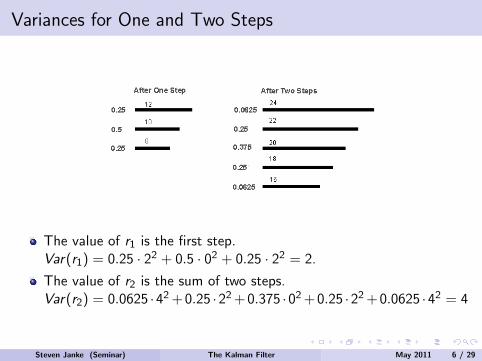
Variances for One and Two Steps

The value of r1 is the first step.Var(r1) = 0.25 · 22 + 0.5 · 02 + 0.25 · 22 = 2.

The value of r2 is the sum of two steps.Var(r2) = 0.0625 ·42 +0.25 ·22 +0.375 ·02 +0.25 ·22 +0.0625 ·42 = 4


Variance Properties

Definition (Variance)

Suppose we have a random variable X with mean µ. Then

Var(X ) =∑x

(x − µ)2P[X = x ]

Note that Var(aX ) = a2Var(X ).

If X and Y are independent random variables:

Var(X + Y ) = Var(X ) + Var(Y )Var(X − Y ) = Var(X ) + Var(Y )

If X and Y are not independent random variables:

Cov(X ,Y ) =∑

x(x − µX )(y − µY )P[X = x ,Y = y ]Var(X + Y ) = Var(X ) + 2Cov(X ,Y ) + Var(Y )


Normal Density

f (x) = 1σ√

2πe−

(x−µ)2

2σ2


Comparing Variances for the Normal Density


Estimators for Robot Position

Suppose that in one step, the robot moves on average 10 cm. Noisein the process makes r1 a little different. Nevertheless, our predictionis r1 = 10.

The robot has an ultrasonic sensor for measuring distance. Againbecause of noise, the reading is not totally accurate, but we have asecond estimate of r1, namely s1.

Both the process noise and the sensor noise are random variables withmean zero. Their variances may not be equal.


The Model and Estimates

The Model

Process: rt = rt−1 + d + Pnt (d is mean distance of one step)

Sensor: st = rt + Snt

The noise random variables Pnt and Snt are normal with mean 0.

The variances of Pnt and Snt are σ2p and σ2

s .

The Estimates

Process: rt = rt−1 + d

Sensor: st = rt + Snt

Error variance: Var(r1 − r1) = σ2p and Var(st − rt) = σ2

s


A Better Estimate

r1 is an estimate of where the robot is after one step (r1).

s1 is also an estimate of r1.

The estimator errors have variances σ2p and σ2

s respectively.

Example (Combine the Estimators)

One way to combine the information in both estimators is to take a linearcombination:

r∗1 = (1− K )r1 + Ks1


Finding the Best K

Our new estimator is r∗1 = (1− K )r1 + Ks1.

A good estimator has small error variance.

Var(r∗1 − r1) = (1− K )2Var(r1 − r1) + K 2Var(s1 − r1)

Substituting gives Var(r∗1 − r1) = (1− K )2σ2p + K 2σ2

s . To minimize thevariance, take the derivative with respect to K and set to zero:

−2(1− K )σ2p + 2Kσ2

s = 0 =⇒ K =σ2

p

σ2p + σ2

s

Definition

K is called the Kalman Gain.


Smaller Variance

With the new K, the error variance of r∗1 is:

Var(r∗1 − r1) = Var((1−

σ2p

σ2p + σ2

s

)(r1 − r1) + (σ2

p

σ2p + σ2

s

)(s1 − r1))

(1)

=( σ2

s

σ2p + σ2

s

)2(σ2

p) +( σ2

p

σ2p + σ2

s

)2(σ2

s ) (2)

=σ2

pσ2s

σ2p + σ2

s

= (1− K )Var(r1 − r1) (3)

Note that Var(r∗1 − r1) is less than both Var(r1− r1) and Var(s1− r1).

Note the new estimator is r∗1 = r1 + K (s1 − r1)


The Kalman Filter

Now we can devise an algorithm:

Prediction:

Add the next step to our last estimate: rt = r∗t−1 + d

Add in variance of next step: Var(rt − rt) = Var(r∗t−1 − rt) + σ2p

Update: (After Sensor Reading)

Minimize: K = Var(rt − rt)/(Var(rt − rt) + σ2s )

Update the position estimate: r∗t = rt + K (st − rt)

Update the variance: Var(r∗t − rt) = (1− K )Var(rt − rt)


Calculating Estimates

Time rt rt Var(rt) K s(t) r∗t Var(r∗t )

0 0 0 0 0 0 0 1000

1 1 1.00 1001 0.99 1.34 1.34 5.96

2 2 2.34 6.96 0.54 0.59 1.40 3.22

3 3 2.40 4.22 0.41 4.28 3.18 2.48


Moving Robot (Step Distance = 1)


Another Look at the Good Estimator

The distribution of rt is normal with density 1σp

√2π

e− (rt−rt )2

2σ2p

The distribution of st is normal with density 1σs

√2π

e− (st−rt )2

2σ2s

The likelihood function is the product of these two densities.Maximizing this likelihood gives a good estimator.

To maximize likelihood, we minimize the negative of the exponent:

(rt − rt)2

2σ2p

+(st − rt)

2

2σ2s

Again use calculus to discover:

rt = (1− K )rt + Kst where K =σ2

p

σ2p + σ2

s


Two-Dimensional Problem

Example

Suppose the state of the robot is both a position and a velocity. Then the

robot state is a vector: rt =

[pt

vt

].

The process is now: rt =

[pt

vt

]=

[1 10 1

] [pt−1

vt−1

]= Frt−1

The sensor reading now looks like this: st =[1 0

] [pt

vt

]= Hrt


Covariance Matrix

With two parts to the robot’s state, a variance in one may affect thevariance in the other. So we define the covariance between two randomvariables X and Y.

Definition (Covariance)

The covariance between random variables X and Y isCov(X ,Y ) =

∑(x − µX )(y − µY )P[X = x ,Y = y ].

Definition (Covariance Matrix)

The covariance matrix for our robot state is

Var(rt) =

[Var(pt) Cov(pt , vt)

Cov(vt , pt) Var(vt)

].


2D Kalman Filter

The two dimensional Kalman Filter gives the predictions and updates interms of matrices:

Prediction:

Add the next step to our last estimate: rt = F r∗t−1

Add in variance of next step:Var(rt − rt) = FVar(r∗t−1 − rt)F

T + Var(rt − rt)

Update:

Gain: K = Var(rt − rt)HT ((HVar(rt − rt)H

T + Var(st − rt))−1

Update the position estimate: r∗t = rt + K (st − Hrt)

Update the variance: Var(r∗t − rt) = (I − KH)Var(rt − rt)


Two-Dimensional Example

Example

Process: rt = Frt−1 where F =

[1 10 1

]Process Covariance matrix:

[Q/3 Q/2Q/2 Q

]Sensor: st =

[1 0

] [pt

vt

]= Hrt

itial State: r0 =

[p0

v0

]=

[00

]


2D Graph Results


Linear Algebra Interpretation

Inner Product: (u, v) = E [(u −mu)T (v −mv )].(Orthogonal = uncorrelated)


Kalman Filter Summary

Summary of Kalman Filter

Assumptions:

The process model must be a linear model.All errors are normally distributed with mean zero.

Algorithm:

Prediction Step 1: Use the model to find estimate of robot state.Prediction Step 2: Use the model to find variance of estimate.Update Step 1: Calculate Kalman Gain from sensor reading.Update Step 2: Use Gain to update estimate of robot state.Update Step 3: Use Gain to update variance of estimator.

Result: This linear estimator of the robot state is unbiased and hasminimum error variance.


What can go wrong ...

A Bad Model

Suppose we use our original model rt = rt−1 + d + Pnt .

But actually the robot is stationary so the real model is rt = rt−1.

Partial solution: Increase the variance of Pnt .

Not a Linear Model

Suppose our sensor measures distance to the origin in a 2D problem.

The the sensor reading gives us√

x2 + y2.

Consequently, no matrix H exists giving st = Hrt .

Extended Kalman Filter approximates the sensor curve with a straightline. (Taylor Series).


Robot is Stationary


Robot is Stationary: Increase Process Variance


Other Applications

Applications:

Tracking the Stock Market. (Time Series)

Computing an asteroid’s orbit.

Weather forecasting.


the kalman filter - colorado college

Documents