the lambrechts–stanley model of configuration spaces

Invent. math. (2019) 216:1–68https://doi.org/10.1007/s00222-018-0842-9

The Lambrechts–Stanley model of configurationspaces

Najib Idrissi1

Received: 1 December 2016 / Accepted: 15 November 2018 /Published online: 8 December 2018© The Author(s) 2018

Abstract We prove the validity over R of a commutative differential gradedalgebra model of configuration spaces for simply connected closed smoothmanifolds, answering a conjecture of Lambrechts–Stanley. We get as a resultthat the real homotopy type of such configuration spaces only depends on thereal homotopy type of the manifold. We moreover prove, if the dimensionof the manifold is at least 4, that our model is compatible with the action ofthe Fulton–MacPherson operad (weakly equivalent to the little disks operad)when the manifold is framed. We use this more precise result to get a complexcomputing factorization homology of framed manifolds. Our proofs use thesame ideas as Kontsevich’s proof of the formality of the little disks operads.

Mathematics Subject Classification 55R80 · 55P62 · 18D50

Contents

Introduction . . . . . . . . . . . . . . . . . . . . . . . . . . . . . . . . . . . . . . . . . 21 Background and recollections . . . . . . . . . . . . . . . . . . . . . . . . . . . . . . 62 The Hopf right comodule model GA . . . . . . . . . . . . . . . . . . . . . . . . . . . 233 Labeled graph complexes . . . . . . . . . . . . . . . . . . . . . . . . . . . . . . . . 244 From the model to forms via graphs . . . . . . . . . . . . . . . . . . . . . . . . . . . 385 Factorization homology of universal enveloping En-algebras . . . . . . . . . . . . . . 55

B Najib [email protected]://idrissi.eu

1 Institut de Mathématiques de Jussieu-Paris Rive Gauche, Université Paris Diderot, Sor-bonne Paris Cité, CNRS, Sorbonne Université, 75013 Paris, France

123

http://crossmark.crossref.org/dialog/?doi=10.1007/s00222-018-0842-9&domain=pdf

http://orcid.org/0000-0001-7288-6726

2 N. Idrissi

6 Outlook: The case of the 2-sphere and oriented manifolds . . . . . . . . . . . . . . . 60Glossary of notation . . . . . . . . . . . . . . . . . . . . . . . . . . . . . . . . . . . . . 64References . . . . . . . . . . . . . . . . . . . . . . . . . . . . . . . . . . . . . . . . . . 66

Introduction

Let M be a closed smooth n-manifold and consider the ordered configurationspace of k points in M :

Confk(M):={(x1, . . . , xk) ∈ Mk | xi �= x j ∀i �= j}.

Despite their apparent simplicity, configuration spaces remain intriguing.One of the most basic questions that can be asked about them is the following:if a manifold M ′ is obtained from M by continuous deformations, then canConfk(M ′) be obtained from Confk(M) by continuous deformations? That is,does the homotopy type of M determine the homotopy type of Confk(M)?

Without any restriction, this is false: the point {0} is homotopy equivalentto the line R, but Conf2({0}) = ∅ is not homotopy equivalent to Conf2(R) �=∅. One might wonder if the conjecture becomes true if restricted to closedmanifolds. In 2005, Longoni and Salvatore [36] found a counterexample: twoclosed 3-manifolds, given by lens spaces, which are homotopy equivalentbut whose configuration spaces are not. This counterexample is not simplyconnected however. The question of the homotopy invariance of Confk(−) forsimply connected closed manifolds remains open to this day.

Here, we do not work with the full homotopy type. Rather, we restrictourselves to the rational homotopy type. This amounts, in a sense, to forgettingall the torsion.Rational homotopy theory canbe studied fromanalgebraic pointof view [48]. The rational homotopy type of a simply connected space X isfully encoded in a “model” of X , i.e. a commutative differential graded algebra(CDGA) A which is quasi-isomorphic to the CDGA of piecewise polynomialforms A∗

PL(X). Due to technical issues, we will in fact work over R. If M isa smooth manifold, then a real model is a CDGA which is quasi-isomorphic tothe CDGA of de Rham forms Ω∗

dR(M). While this is slightly coarser than therational homotopy type of M , in terms of computations it is often enough.

Thus, our goal is the following: given a model of M , deduce an explicit,small model of Confk(M). This explicit model only depends on the model ofM . This shows the (real) homotopy invariance of Confk(−) on the class ofmanifolds we consider. Moreover, this explicit model can be used to performcomputations, e.g. the real cohomology ring of Confk(M), etc.

We focus on simply connected (thus orientable) closed manifolds. Theysatisfy Poincaré duality. Lambrechts and Stanley [32] showed that anysuch manifold admits a model A which satisfies itself Poincaré duality, i.e.

123

The Lambrechts–Stanley model 3

there is an “orientation” An ε−→ R which induces non-degenerate pairingsAk ⊗ An−k → R for all k. Lambrechts and Stanley [33] built a CDGA GA(k)

out of such a Poincaré duality model (they denote it F(A, k)). If we viewH∗(Confk(R

n)) as spanned by graphs modulo Arnold relations, then GA(k)

consists of similar graphs with connected components labeled by A, and thedifferential splits edges. Lambrechts and Stanley proved that GA(k) is quasi-isomorphic to A∗

PL(Confk(M)) as a dg-module. They conjectured that thisquasi-isomorphism can be enhanced to give a quasi-isomorphism of CDGAs sothat GA(k) defines a rational model of Confk(M). We answer this conjectureby the affirmative in the real setting in the following theorem.

Theorem 1 (Corollary 78) Let M be a simply connected, closed, smooth man-ifold. Let A be any Poincaré duality model of M. Then for all k ≥ 0, GA(k) isa model for the real homotopy type of Confk(M).

Corollary 2 (Corollary 79) For simply connected closed smooth manifolds,the real homotopy type of M determines the real homotopy type of Confk(M).

Over the past decades, attempts weremade to solve the Lambrechts–Stanleyconjecture, and results were obtained for special kinds of manifolds, or forlow values of k. When M is a smooth complex projective variety, Kriz [30]had previously shown that GH∗(M)(k) is actually a rational CDGA model forConfk(M). The CDGA GH∗(M)(k) is the E2 page of a spectral sequence ofCohen–Taylor [9] that converges to H∗(Confk(M)). Totaro [51] has shownthat for a smooth complex compact projective variety, the spectral sequenceonly has one nonzero differential. When k = 2, then GA(2) was known to bea model of Conf2(M) either when M is 2-connected [31] or when dim M iseven [10].

Our approach is different than the ones used in these previous works. Weuse ideas coming from the theory of operads. In particular, we consider theoperad of little n-disks, defined by Boardman–Vogt [4], which consists ofconfiguration spaces of small n-disks (instead of points) embedded insidethe unit n-disk. These spaces of little n-disks are equipped with compositionproducts, which are basically defined by inserting a configuration of l littlen-disks into the i th little disk of a configuration of k little n-disks, resultingin a configuration of k + l − 1 little n-disks. The idea is that a configurationof little n-disks represents an operation acting on n-fold loop spaces, andthe operadic composition products of little n-disks reflect the compositionof such operations. The configuration spaces of little n-disks are homotopyequivalent to the configurations spaces of points in the Euclidean n-space R

n ,but the operadic composition structure does not go through this homotopyequivalence.

In our work, we actually use another model of the little n-disk operads,defined using the Fulton–MacPherson compactifications FMn(k) of the con-

123

4 N. Idrissi

figurations spaces Confk(Rn) [2,19,46]. This compactification allows us to

retrieve, on this collection of spaces FMn = {FMn(k)}, the operadic com-position products which were lost in the configurations spaces Confk(R

n).We also use the Fulton–MacPherson compactifications FMM(k) of the con-figuration spaces Confk(M) associated to a closed manifold M . When M isframed, these compactifications assemble into an operadic right module FMMover the Fulton–MacPherson operad FMn , which roughly means that we caninsert a configuration in FMn into a configuration in FMM . We show that theLambrechts–Stanley model is compatible with this action of the little disksoperad, as we explain now.

The little n-disks operads are formal [18,28,34,43,49]. Kontsevich’s proof[28,34] of this theorem uses the spaces FMn . If we temporarily forget aboutoperads, this formality theorem means in particular that each space FMn(k) is“formal”, i.e. the cohomologye∨

n (k):=H∗(FMn(k)) (with a trivial differential)is a model for the real homotopy type of FMn(k). To prove Theorem 1, wegeneralize Kontsevich’s approach to prove that GA(k) is a model of FMM(k).

To establish his result, Kontsevich has to consider fiberwise integrationsof forms along a particular class of maps, which are not submersions, butrepresent the projection map of “semi-algebraic bundles”. In order to definesuch fiberwise integration operations, Kontsevich uses CDGAs of piecewisesemi-algebraic (PA) forms Ω∗

PA(−) instead of the classical CDGAs of de Rhamforms. The theory of PA forms was developed in [23,29]. Any closed smoothmanifold M is a semi-algebraic manifold [39,50], and the CDGA Ω∗

PA(M) isa model for the real homotopy type of M . For the formality of FMn , a descentargument [22] is available to show that formality over R implies formalityoverQ. However, no such descent argument exists for models with a nontrivialdifferential such as GA. Therefore, although we conjecture that our results onreal homotopy types descend to Q, we have no general argument ensuring thatsuch a property holds.

The cohomology e∨n = H∗(FMn) inherits a Hopf cooperad structure from

FMn , i.e. it is a cooperad (the dual notion of operad) in the category of CDGAs.The CDGAs of forms Ω∗

PA(FMn(k)) also inherit a Hopf cooperad structure (upto homotopy). The formality quasi-isomorphisms between the cohomologyalgebras e∨

n (k) and the CDGAs of forms on FMn(k) are compatible in a suitablesense with this structure. Therefore the Hopf cooperad e∨

n fully encodes therational homotopy type of the operad FMn .

In this paper, we also prove that the Lambrechts–Stanley model GA deter-mines the real homotopy type of FMM as a right module over the operad FMnwhen M is a framed manifold. To be precise, our result reads as follows.

Theorem 3 (Theorem 62) Let M be a framed smooth simply connectedclosed manifold with dim M ≥ 4. Let A be any Poincaré duality modelof M. Then the collection GA = {GA(k)}k≥0 forms a Hopf right e∨

n -

123


comodule. Moreover the Hopf right comodule (GA,e∨n ) is weakly equivalent

to (Ω∗PA(FMM), Ω∗

PA(FMn)).

For dim M ≤ 3, the proof fails (see Proposition 45). However, in this case,the only examples of simply connected closed manifolds are spheres, thanksto Perelman’s proof of the Poincaré conjecture [41,42]. We can then directlyprove that GA(k) is a model for Confk(M) (see Sect. 4.3).

Our proof of Theorem 3, which is inspired by Kontsevich’s proof of theformality of the little disks operads, is radically different from the proofsof [33]. It involves an intermediary Hopf right comodule of labeled graphsGraphsR . This comodule is similar to a comodule recently studied byCampos–Willwacher [6], which corresponds to the case R = S(H∗(M)).Note however that the approach of Campos–Willwacher differs from ours.In comparison to their work, our main contribution is the definition of thequasi-isomorphism between the CDGAsΩ∗

PA(FMM(k)) and the small, explicitLambrechts–Stanley model GA(k), which has the advantage of being finite-dimensional and much more computable than GraphsS(H(M))

(k).

Applications. Ordered configuration spaces appear in many places in topologyand geometry. Therefore, thanks to Theorems 1 and 3, the explicitmodelGA(k)

provides an efficient computational tool in many concrete situations.To illustrate this, we show how to apply our results to compute factorization

homology, an invariant of framed n-manifolds defined from an En-algebra [3].Let M be a framed manifold with Poincaré duality model A, and B be an n-Poisson algebras, i.e. an algebra over the operad H∗(En). Our results shows thatwe can compute the factorization homology of M with coefficients in B justfrom GA and B. As an application, we compute factorization homology withcoefficients in a higher enveloping algebra of a Lie algebra (Proposition 81),recovering a theorem of Knudsen [27].

The Taylor tower in the Goodwillie–Weiss calculus of embeddings may becomputed in a similar manner [5,21]. It follows from a result of [52, Section5.1] that FMM may be used for this purpose. Therefore our theorem shows thatGA may also be used for computing this Taylor tower.

Roadmap. In Sect. 1, we lay out our conventions and recall the necessarybackground. This includes dg-modules and CDGAs, (co)operads and their(co)modules, semi-algebraic sets and PA forms. We also recall basic resultson the Fulton–MacPherson compactifications of configuration spaces FMn(k)

and FMM(k), and the main ideas of Kontsevich’s proof of the formality of thelittle disks operads using the CDGAs of PA forms on the spaces FMn(k). Weuse the formalism of operadic twisting, which we recall, to deal with signsmore easily. Finally, we recollect the necessary background on Poincaré dual-ity CDGAs and the Lambrechts–Stanley CDGAs. In Sect. 2, we build out of theLambrechts–Stanley CDGAs a Hopf right e∨

n -comodule GA.

123

6 N. Idrissi

In Sect. 3, we construct the labeled graph complex GraphsR which will beused to connectGA toΩ∗

PA(FMM). The construction is inspired byKontsevich’sconstruction of the unlabeled graph complex Graphsn . It is done in severalsteps. The first step is to consider a graded module of labeled graphs, GraR .In order to be able to map GraR intoΩ∗

PA(FMM), we recall the construction ofwhat is called a “propagator” in the mathematical physics literature. We then“twist” GraR to obtain a new object TwGraR , which consists of graphs withtwo kinds of vertices: “external” and “internal”. Finally we must reduce ourgraphs to obtain a new object, GraphsR , by removing all the connected com-ponents with only internals vertices in the graphs using a “partition function”(a function which resembles the Chern–Simons invariants).

In Sect. 4, we prove that the zigzag of Hopf right comodule morphismsbetween GA andΩ∗

PA(FMM) is a weak equivalence. We first connect our graphcomplex GraphsR to the Lambrechts–Stanley CDGAs GA. This requires van-ishing results about the partition function. Thenwe end the proof of the theoremby showing that all the morphisms are quasi-isomorphisms. Finally we studythe cases S2 and S3.

In Sect. 5, we use our model to compute factorization homology of framedmanifolds and we compare the result to a complex obtained by Knudsen. InSect. 6 we work out a variant of our theorem for the only simply connectedsurface using the formality of the framed little 2-disks operad, and we presenta conjecture about higher dimensional oriented manifolds.

For convenience, we provide a glossary of our main notations at the end ofthis paper.

1 Background and recollections

1.1 DG-modules and CDGAs

We consider differential graded modules (dg-modules) over the base field R.Unless otherwise indicated, (co)homology of spaces is considered with realcoefficients. All our dg-modules will have a cohomological grading, V =⊕

n∈ZV n . All the differentials raise degrees by one: deg(dx) = deg(x) + 1.

We say that a dg-module is of finite type if it is finite dimensional in eachdegree. Let V [k] be the desuspension, defined by (V [k])n = V n+k . Fordg-modules V, W and homogeneous elements v ∈ V, w ∈ W , we let(v ⊗ w)21:=(−1)(deg v)(degw)w ⊗ v and we extend this linearly to the ten-sor product. Moreover, given an element X ∈ V ⊗ W , we will often use avariant of Sweedler’s notation to express X as a sum of elementary tensors,X :=∑

(X) X ′ ⊗ X ′′ ∈ V ⊗ W .

123


We call CDGAs the (graded) commutative unital algebras in dg-modules. Ingeneral, for a CDGA A, we let μA : A⊗2 → A be its product. For a dg-moduleV , we let S(V ) be the free unital symmetric algebra on V .

We will need a model category structure on the category of CDGAs. We usethemodel category structure given by the general result of [24] for categories ofalgebras over operads. Theweak equivalences are the quasi-isomorphisms, thefibrations are the surjective morphisms, and the cofibrations are characterizedby the left lifting property with respect to acyclic fibrations. A path object forthe initial CDGA R is given by A∗

PL(Δ1) = S(t, dt), the CDGA of polynomials

forms on the interval. It is equipped with an inclusion R ↪∼−→ A∗

PL(Δ1), and

two projections ev0, ev1 : A∗PL(Δ1)

∼−→ R given by setting t = 0 or t = 1.Two morphisms f, g : A → B with cofibrant source are homotopic if thereexists a homotopy h : A → B ⊗ A∗

PL(Δ1) such that the following diagramcommutes:

A

B B ⊗ A∗PL(Δ1) B

fh

g

id⊗ ev0

∼id⊗ ev1

∼.

Many of the CDGAs that appear in this paper are Z-graded. However, todeserve the name “model of X”, a CDGA should be connected to A∗

PL(X) onlyby N-graded CDGAs. The next proposition shows that considering this largercategory does not change our statement.

Proposition 4 Let A, B be two N-graded CDGAs which are homologicallyconnected, i.e. H0(A) = H0(B) = R. If A and B are quasi-isomorphic asZ-graded CDGAs, then they also are as N-graded CDGAs.

Proof This follows from the results of [17, §II.6.2]. Let us temporarily denotecdgaN the category of N-graded CDGAs (dg∗Com in [17]) and cdgaZ thecategory of Z-graded CDGAs (dgCom in [17]). Note that in [17], Z-gradedCDGAs are homologically graded, but we can use the usual correspondenceAi = A−i to keep our convention that all dg-modules are cohomologicallygraded. There is an obvious inclusion ι : cdgaN → cdgaZ, which clearlydefines a full functor that preserves and reflects quasi-isomorphisms.

Let Bm be the dg-module R concentrated in degree m, let E

m be the dg-module given by two copies of R in respective degree m − 1 and m suchthat dEm is the identity of R in these degrees (hence E

m is acyclic), and leti : B

m → Em be the obvious inclusion. Themodel category cdgaN is equipped

with a set of generating cofibrations given by the morphisms S(i) : S(Bm) →S(Em) and of the morphism ε : S(B0) → R. Recall that a cellular complexof generating cofibrations is a CDGA obtained by a sequential colimit R =colimk R〈k〉, where R〈0〉 = R and R〈k+1〉 is obtained from R〈k〉 by a pushout

123

8 N. Idrissi

of generating cofibrations along attaching maps h : S(Bm) → R〈k〉. In [17,§II.6.2], the expression “connected generating cofibrations” is used for thegenerating cofibrations of the form S(i) : S(Bm) → S(Em) with m > 0.

In the proof of [17, Proposition II.6.2.8], it is observed that, if A is homo-logically connected, then the attaching map h : S(B0) → A associated to agenerating cofibration ε : S(B0) → R necessarily reduces to the augmenta-tion ε : S(B0) → R followed by the inclusion as the unit R ⊂ A. Thus apushout of the generating cofibration ε : S(B0) → R reduces to a neutraloperation in this case. In the proof of [17, Proposition II.6.2.8], it is deducedfrom this observation that any homologically connected algebra admits a res-olution RA

∼−→ A such that RA is a cellular complex of connected generatingcofibrations. Connected generating cofibrations are also cofibrations in cdgaZ

after applying ι. Moreover ι preserves colimits. It follows that ιRA is cofibrantin cdgaZ too.

By hypothesis, ιA and ιB areweakly equivalent in cdgaZ, hence ιRA and ιBare also weakly equivalent (because ι clearly preserves quasi-isomorphisms),through a zigzag ιRA

∼←− · ∼−→ ιB. As ιRA is cofibrant (and all CDGAs arefibrant), we can find a direct quasi-isomorphism ιRA

∼−→ ιB and therefore azigzag ιA

∼←− ιRA∼−→ ιB which only involves N-graded CDGAs. ��

1.2 (Co)operads and their right (co)modules

We assume basic proficiency with Hopf (co)operads and (co)modules over(co)operads, see e.g. [16,17,35].We indexour (co)operads byfinite sets insteadof integers to ease the writing of some formulas. If W ⊂ U is a subset, wewrite the quotient U/W = (U\W ) � {∗}, where ∗ represents the class ofW ; note that U/∅ = U � {∗}. An operad in dg-modules, for instance, isgiven by a functor from the category of finite sets and bijections (a symmetriccollection) P : U �→ P(U ) to the category of dg-modules, together with a unitk → P({∗}) and composition maps ◦W : P(U/W )⊗P(W ) → P(U ) for everypair of sets W ⊂ U , satisfying the usual associativity, unity and equivarianceconditions. Dually, a cooperad C is given by a symmetric collection, a counitC({∗}) → k, and cocomposition maps ◦∨

W : C(U ) → C(U/W ) ⊗ C(W ) forevery pair W ⊂ U .

Let k = {1, . . . , k}. We recover the usual notion of a cooperad indexed bythe integers by considering the collection {C(k)}k≥0, and the cocompositionmaps ◦∨

i : C(k + l − 1) → C(k) ⊗ C(l) corresponds to ◦∨{i,...,i+l−1}.Following Fresse [17, §II.9.3.1], a “Hopf cooperad” is a cooperad in the

category of CDGAs. We do not assume that (co)operads are trivial in arity zero,but they will satisfy P(∅) = k (resp. C(∅) = k). Therefore we get (co)operadstructures equivalent to the structure of Λ-(co)operads considered by Fresse

123


[17, §II.11], which he uses to model rational homotopy types of operads inspaces satisfying P(0) = ∗ (but we do not use this formalism in the sequel).

The result of Proposition 4 extends to Hopf cooperads (and to Hopf Λ-cooperads). To establish this result, we still use a description of generatingcofibrations of N -graded Hopf cooperads, which are given by morphisms ofsymmetric algebras of cooperads S(i) : S(C) → S(D), where i : C →D is a dg-cooperad morphism that is injective in positive degrees (see [17,§II.9.3] for details). In the context of homologically connected cooperads,we can check that the pushout of such a Hopf cooperad morphism along anattaching map reduces to a pushout of a morphism of symmetric algebras ofcooperads S(C/ ker(i)) → S(D), where we mod out by the kernel of the mapi : C → D in degree 0.Wededuce from this observation that any homologicallyconnected N -graded Hopf cooperad admits a resolution by a cellular complexof generating cofibrations of the form S(i) : S(C) → S(D), where themap i isinjective in all degrees (we again call such a generating cofibration connected).The category of Z-graded Hopf cooperads inherits a model structure, like thecategory of N-graded Hopf cooperads considered in [17, §II.9.3]. Cellularcomplexes of connected generating cofibrations of N-graded Hopf cooperadsdefine cofibrations in the model category of Z-graded Hopf cooperads yet, asin the proof of Proposition 4.

Given an operad P, a right P-module is a symmetric collection M equippedwith composition maps ◦W : M(U/W ) ⊗ P(W ) → M(U ) satisfying the usualassociativity, unity and equivariance conditions. A right comodule over a coop-erad is defined dually. If C is a Hopf cooperad, then a right Hopf C-comoduleis a C-comodule N such that all the N(U ) are CDGAs and all the maps ◦∨

W aremorphisms of CDGAs.

Definition 5 Let C (resp. C′) be a Hopf cooperad and N (resp. N′) be a Hopfright comodule over C (resp. C′). A morphism of Hopf right comodules is apair ( fN, fC) consisting of a morphism of Hopf cooperads fC : C → C′, anda map of Hopf right C′-comodules fN : N → N′, where N has the C-comodulestructure induced by fC. It is a quasi-isomorphism if both fC and fN are quasi-isomorphisms in each arity. A Hopf right C-module N is said to be weaklyequivalent to a Hopf right C′-module N′ if the pair (N,C) can be connected tothe pair (N′,C′) through a zigzag of quasi-isomorphisms.

The next very general lemma can for example be found in [6, Section 5.2].Let C be a cooperad, and see the CDGA A as an operad concentrated in arity1. Recall that C ◦ A = ⊕

i≥0 C(i) ⊗Σi A⊗i denotes the composition productof operads, where we view A as an operad concentrated in arity 1. Then thecommutativity of A implies the existence of a distributive law t : C◦A → A◦C,given in each arity by the morphism t : C(n) ⊗ A⊗n → A ⊗ C(n) given byx ⊗ a1 ⊗ · · · ⊗ an �→ a1 . . . an ⊗ x .

123

10 N. Idrissi

Lemma 6 Let N be a right C-comodule, and see A as an operad concentratedin arity 1. Then N ◦ A is a right C-comodule through the map:

N ◦ AΔN◦1−−−→ N ◦ C ◦ A

1◦t−→ N ◦ A ◦ C. ��

1.3 Semi-algebraic sets and forms

Kontsevich’s proof of the formality of the little disks operads [28] uses thetheory of semi-algebraic sets, as developed in [23,29]. A semi-algebraic setis a subset of R

N defined by finite unions of finite intersections of zero setsof polynomials and polynomial inequalities. By the Nash–Tognoli Theorem[39,50], any closed smooth manifold is algebraic hence semi-algebraic.

There is a functor Ω∗PA of “piecewise semi-algebraic (PA) differential

forms”, analogous to deRham forms. If X is a compact semi-algebraic set, thenΩ∗

PA(X) � A∗PL(X) ⊗Q R, i.e. the CDGA Ω∗

PA(X) models the real homotopytype of X [23, Theorem 6.1].

A key feature of PA forms is that it is possible to compute integrals of“minimal forms” along fibers of “PA bundles”, i.e. maps with local semi-algebraic trivializations [23, Section 8]. Aminimal form is of the type f0d f1∧· · · ∧ d fk where fi : M → R are semi-algebraic maps. Given such a minimalform λ and a PA bundle p : M → B with fibers of dimension r , there is anew form (which is not minimal in general), also called the pushforward of λ

along p:

p∗λ:=∫

p:M→Bλ ∈ Ωk−r

PA (B).

In what follows, we use an extension of the fiberwise integration of minimalforms to the sub-CDGA of “trivial forms” given in [6, Appendix C]. Brieflyrecall that trivial forms are integrals of minimal forms along fibers of a trivialPA bundle (see [6, Definition 81]). In fact, in Sect. 3.3, we consider a certainform, the “propagator”, which is not minimal but trivial in this sense, and weapply the extension of the fiberwise integration to this form.

The functorΩ∗P A is monoidal, but not stronglymonoidal, and contravariant.

Thus, given an operad P in semi-algebraic sets, Ω∗PA(P) is an “almost” Hopf

cooperad and satisfies a slightly modified version of the cooperad axioms,as explained in [34, Definition 3.1]. Cooperadic structure maps are replaced

by zigzags Ω∗PA(P(U ))

◦∗W−→ Ω∗

PA(P(U/W ) × P(W ))∼←− Ω∗

PA(P(U/W )) ×Ω∗

PA(P(W )) (where the second map is the Künneth morphism). If C is a Hopfcooperad, an “almost” morphism f : C → Ω∗

PA(P) is a collection of CDGA

123


morphisms fU : C(U ) → Ω∗PA(P(U )) for all U , such that the following

diagrams commute:

C(U ) C(U/W ) ⊗ C(W )

Ω∗PA(P(U )) Ω∗

PA(P(U/W ) × P(W )) Ω∗PA(P(U/W )) ⊗ Ω∗

PA(P(W ))

◦∨W

fU fU/W ⊗ fW◦∗W ∼

Similarly, ifM is aP-module, thenΩ∗PA(M) is an “almost” Hopf right comodule

overΩ∗PA(P). If N is a Hopf right C-comodule, where C is a cooperad equipped

with an “almost” morphism f : C → Ω∗PA(P), then an “almost” morphism g :

N → Ω∗PA(M) is a collection of CDGA morphisms gU : N(U ) → Ω∗

PA(M(U ))

that make the following diagrams commute:

N(U ) N(U/W ) ⊗ C(W )

Ω∗PA(M(U )) Ω∗

PA(M(U/W ) × P(W )) Ω∗PA(M(U/W )) ⊗ Ω∗

PA(P(W ))

◦∨W

gU gU/W ⊗ fW◦∗W ∼

We will generally omit the adjective “almost”, keeping in mind that somecommutative diagrams are a bit more complicated than at first glance.

Remark 7 There is a construction Ω∗ that turns a simplicial operad P into a

Hopf cooperad and such that a morphism of Hopf cooperads C → Ω∗ (P)

is the same thing as an “almost” morphism C → A∗PL(P), where A∗

PL is thefunctor of Sullivan forms [17, Section II.10.1]. Moreover there is a canonicalcollection of maps (Ω∗

(P))(U ) → A∗PL(P(U )), which are weak equivalences

if P is a cofibrant operad. This functor is built by considering the right adjointof the functor on operads induced by the Sullivan realization functor, whichis monoidal. A similar construction can be extended to Ω∗

PA and to modulesover operads. This construction allows us to make sure that the cooperads andcomodules we consider truly encode the rational or real homotopy type of theinitial operad or module (see [17, §II.10.2]).

1.4 Little disks and related objects

The little disks operad En is a topological operad initially introduced by Mayand Boardman–Vogt [4,37] to study iterated loop spaces. Its homology en :=H∗(En) is described by a theoremofCohen [8]: it is either the operad governingassociative algebras for n = 1, or n-Poisson algebras for n ≥ 2. We alsoconsider the linear dual e∨

n :=H∗(En), which is a Hopf cooperad.In fact, we use the Fulton–MacPherson operad FMn , which is an operad

in spaces weakly equivalent to the little disks operad En . The componentsFMn(k) are compactifications of the configuration spaces Confk(R

n), defined

123

12 N. Idrissi

by using a real analogue due to Axelrod–Singer [2] of the Fulton–MacPhersoncompactifications [19]. The idea of this compactification is to allow configu-rations where points become “infinitesimally close”. Then one uses insertionof such infinitesimal configurations to define operadic composition productson the spaces FMn(k). We refer to [46] for a detailed treatment and to [34,Sections 5.1–5.2] for a clear summary. In both references, the name C[k] isused for what we call FMn(k).

The first two spaces FMn(∅) = FMn(1) = ∗ are singletons, and FMn(2) =Sn−1 is a sphere. We let the volume form of FMn(2) be:

voln−1 ∈ Ωn−1PA (Sn−1) = Ωn−1

PA (FMn(2)) (1)

The spaceFMn(k) is a semi-algebraic stratifiedmanifold, of dimension nk−n − 1 for k ≥ 2, and of dimension 0 otherwise. For u �= v ∈ U , we candefine the projection maps that forget all but two points in the configuration,puv : FMn(U ) → FMn(2). These projections are semi-algebraic bundles.If M is a manifold, the configuration space Confk(M) can similarly be

compactified to give a space FMM(k). By forgetting points, we again obtainprojection maps, for u, v ∈ U :

pu : FMM(U ) � FMM(1) = M, puv : FMM(U ) � FMM(2). (2)

The two projections p1 and p2 are equal when restricted ∂FMM(2), and theydefine a sphere bundle of rank n − 1,

p : ∂FMM(2) � M. (3)

When M is framed, the collection of spaces FMM assemble to form atopological right module over FMn , with composition products defined byinsertion of infinitesimal configurations. Moreover in this case, the spherebundle p : ∂FMM(2) → M is trivialized by:

M × Sn−1 ∼= FMM(1) × FMn(2)◦1−→ ∂FMM(2). (4)

Recall fromSect. 1.3 thatwe can endow M with a semi-algebraic structure. Itis immediate that FMM(k) is a stratified semi-algebraic manifold of dimensionnk. Moreover, the proofs of [34, Section 5.9] can be adapted to show that theprojections pU : FMM(U � V ) → FMM(U ) are PA bundles.

123


1.5 Operadic twisting

We will make use of the “operadic twisting” procedure in what follows [11].Let us now recall this procedure, in the case of cooperads.

Let Lien be the operad governing shifted Lie algebras. A Lien-algebra isa dg-module g equipped with a Lie bracket [−, −] : g⊗2 → g[1−n] of degree1 − n, i.e. we have [gi , g j ] ⊂ gi+ j+(1−n).

Remark 8 The degree convention is such that there is an embedding of operadsLien → H∗(FMn), i.e. Poisson n-algebras are Lien-algebras. The usual Lieoperad is Lie1. This convention is consistent with [53]. However in [54], thenotation is Lie(n) = Lien+1. In [11], only the unshifted operad Lie = Lie1is considered.

The operad Lien is quadratic Koszul (see e.g. [35, Section 13.2.6]), andas such admits a cofibrant resolution hoLien:=Ω(K (Lien)), where Ω isthe cobar construction and K (Lien) is the Koszul dual cooperad of Lie.Algebras over hoLien are (shifted) L∞-algebras, also known as homotopyLie algebras, i.e. dg-modules g equipped with higher brackets [−, . . . , −]k :g⊗k → g[3 − k − n] (for k ≥ 1) satisfying the classical L∞ equations.

Let C be a cooperad (with finite-type components in each arity) equippedwith a map to the dual of hoLien . This map can equivalently be seen as aMaurer–Cartan element in the following dg-Lie algebra [35, Section 6.4.2]:

HomΣ(K (Lien),C∨):=

(∏

i≥0

(C∨(i) ⊗ R[−n]⊗i)Σi [n], ∂, [−, −]

)

, (5)

where we used the explicit description of theKoszul dual K (Lien) as a shiftedversion of the cooperad encoding cocommutative coalgebras. Given f, g ∈HomΣ(K (Lien),C∨), their bracket is [ f, g] = f � g ∓ g � f , where � isgiven by:

f � g : K (Lien)cooperad−−−−−→ K (Lien) ◦ K (Lien)

f ◦g−−→ C∨ ◦ C∨ operad−−−→ C∨.

An element μ ∈ HomΣ(K (Lien),C∨) is said to satisfy the Maurer–Cartanequation if ∂μ + μ � μ = 0. Such an element is called a twisting morphism in[35, Section 6.4.3], and the equivalence with morphisms hoLien → C∨ (ordually C → hoLie∨

n ) is [35, Theorem 6.5.7]. In the sequel, we will alternatebetween the two points of view, morphisms or Maurer–Cartan elements.

There is an action of the symmetric groupΣi on i = {1, . . . , i}. As a gradedmodule, the twist of C with respect to μ is given by:

TwC(U ) :=⊕

i≥0

(C(U � i) ⊗ R[n]⊗i)

Σi. (6)

123

14 N. Idrissi

The symmetric collection TwC inherits a cooperad structure from C. Thedifferential of TwC is the sumof the internal differential ofCwith a differentialcoming from the action ofμ that we now explain. The action ofμ is threefold,and the total differential of TwC(U ) can be expressed as:

dTwC:=dC + (− · μ) + (− · μ1) + (μ1 · −). (7)

Let us now explain these notations. Let i ≥ 0 be some fixed integer and let usdescribe the action of μ on C(U � i) ⊂ TwC(U ) (up to degree shifts). In whatfollows, for a set J ⊂ i , we let j :=#J , and i/J ∼= i + j − 1.

Recall that μ is a formal sum of elements C( j)∨ for j ≥ 0. The first action(− · μ) is the sum over all subsets J ⊂ i of the following cocompositions:

C(U � i)◦∨

J−→ C(U � i/J )

⊗C(J )id⊗μ−−−→ C(U � i/J ) ⊗ R ∼= C(U � i + j − 1). (8)

For the two other terms, we need the element μ1 ∈ ∏j≥0 C( j � {∗})∨. It is

the sum over all possible ways of distinguishing one input of μ in each arity.(Distinguishing one input does not respect the invariants in the definition ofEq. (5), but taking the sum over all possible ways does.)

The second action (−·μ1) is then the sum of the following cocompositions,over all subsets J ⊂ i and over all ∗ ∈ U (where we use the obvious bijectionU/{∗} ∼= U ):

C(U � i)◦∨{u}�J−−−→ C

((U � i)/({∗} � J )

)

⊗C({∗} � J )id⊗μ1−−−−→ C(U � i + j − 1), (9)

Finally, the third action (μ1 · −) is the sum over all subsets J ⊂ i of thecocompositions (where we use the obvious bijection (U � I )/(U � J ) ={∗} � I\J ):

C(U � i)◦∨

U�J−−−→ C({∗} � i\J ) ⊗ C(U � J )μ1⊗id−−−→ C(U � J ), (10)

Lemma 9 If C is a Hopf cooperad satisfying C(∅) = k, then TwC inherits aHopf cooperad structure.

Proof To multiply an element of C(U � I ) ⊂ TwC(U ) with an element of

C(U � J ) ⊂ TwC(U ), we use the maps C(V )◦∨

∅−→ C(V/∅) ⊗ C(∅) ∼=C(V � {∗}) iterated several times, to obtain elements in C(U � I � J ) and theproduct. ��

123


Moreover, we will need to twist right comodules over cooperads. This con-struction is found (for operads) in [54, Appendix C.1]. Let us fix a cooperad Cand a twist TwC with respect to μ as above. Given a right C-comodule M, wecan also twist it with respect to μ, as follows. As a graded module, the objectTwM(U ) is defined by:

TwM(U ):=∏

i≥0

(M(U � i) ⊗ (R[n])⊗i)

Σi.

The comodule structure is inherited from M. The total differential is the sum:

dTwM:=dM + (− · μ) + (− · μ1), (11)

where (− · μ) and (− · μ1) are as in Eqs. (8) and (9) but using the comodulestructure. Note that M is only a right module, so there can be no term (μ1 · −)

in this differential. Lemma 9 has an immediate extension:

Lemma 10 If C is a Hopf cooperad satisfying C(∅) = k and M is a Hopf rightC-comodule, then TwM inherits a Hopf right (TwC)-comodule structure. ��

1.6 Formality of the little disks operad

Kontsevich’s proof of the formality of the little disks operads [28, Section 3],can be summarized by the fact that Ω∗

PA(FMn) is weakly equivalent to e∨n as a

Hopf cooperad. For detailed proofs, we refer to [34].We outline this proof here as we will mimic its pattern for our theorem. The

idea of the proof is to construct a Hopf cooperad Graphsn . The elements ofGraphsn are formal linear combinations of special kinds of graphs, with twotypes of vertices, numbered “external” vertices and unnumbered “internal”vertices. The differential is defined combinatorially by edge contraction. It isbuilt in such a way that there exists a zigzag e∨

n∼←− Graphsn

∼−→ Ω∗PA(FMn).

The first map is the quotient by the ideal of graphs containing internal ver-tices. The second map is defined using integrals along fibers of the PA bundlesFMn(U � I ) → FMn(U ) which forget some points in the configuration. Aninduction argument shows that the first map is a quasi-isomorphism, and thesecond map is easily seen to be surjective on cohomology.

In order to deal with signs more easily, we use (co)operadic twisting(Sect. 1.5). Thus the Hopf cooperad Graphsn is not the same as the Hopfcooperad D from [34], see Remark 13.

The cohomology of En . The cohomologye∨n (U ) = H∗(En(U )) has a classical

presentation due to Arnold [1] and Cohen [8]. We have

e∨n (U ) = S(ωuv)u,v∈U /I, (12)

123

16 N. Idrissi

where the generators ωuv have cohomological degree n − 1, and the ideal Iencoding the relations is generated by the polynomials (called Arnold rela-tions):

ωuu = 0; ωvu = (−1)nωuv; ω2uv = 0; ωuvωvw + ωvwωwu + ωwuωuv = 0. (13)

The cooperadic structure maps are given by (where [u], [v] ∈ U/W are theclasses of u and v in the quotient):

◦∨W : e∨

n (U ) → e∨n (U/W ) ⊗ e∨

n (W ), ωuv �→{1 ⊗ ωuv, if u, v ∈ W ;ω[u][v] ⊗ 1, otherwise.

(14)

Graphs with only external vertices. The intermediary cooperad of graphs,Graphsn , is built in several steps. In the first step, define a cooperad of graphswith only external vertices, with generators euv of degree n − 1:

Gran(U ) = (S(euv)u,v∈U /(e2uv = euu = 0, evu = (−1)neuv), d = 0

).

(15)

The definition of Gran(U ) is almost identical to the definition of e∨n (U ),

except that we do not kill the Arnold relations.The CDGA Gran(U ) is spanned by words of the type eu1v1 . . . eur vr . Such

a word can be viewed as a graph with U as the set of vertices, and an edgebetween ui and vi for each factor eui vi . For example, euv is a graphwith a singleedge from u to v (see Eq. (16) for another example). Edges are oriented, butfor even n an edge is identified with its mirror (so we can forget orientations),while for odd n it is identified with the opposite of its mirror. In pictures, we donot draw orientations, keeping in mind that for odd n, they are necessary to getprecise signs. Graphs with double edges or edges between a vertex and itselfare set to zero. Given such a graph, its set of edges EΓ ⊂ (U

2

)is well-defined.

The vertices of these graphs are called “external”, in contrast with the internalvertices that are going to appear in the next part.

e12e13e56 =1 2

3 4

5

6

∈ Gran(6) (16)

The multiplication of the CDGA Gran(U ), from this point of view, consistsof gluing two graphs along their vertices. The cooperadic structure map ◦∨

W :Gran(U ) → Gran(U/W ) ⊗ Gran(W ) maps a graph Γ to ±ΓU/W ⊗ ΓW

123


such that ΓW is the full subgraph of Γ with vertices W and ΓU/W collapsesthis full subgraph to a single vertex. On generators, ◦∨

W is defined by a formulawhich is in fact identical to Eq. (14), replacing ωuv by euv. This implies thatthe cooperad Gran maps to e∨

n by sending euv to ωuv .There is a morphism ω′ : Gran → Ω∗

PA(FMn) given on generators by:

ω′ : Gran(U ) → Ω∗PA(FMn(U )), Γ �→

∧

(u,v)∈EΓ

p∗uv(voln−1), (17)

where puv : FMn(U ) → FMn(2) is the projection map defined in Sect. 1.4,and voln−1 is the volume form of FMn(2) ∼= Sn−1 from Eq. (1).

Twisting. The second step of the construction is cooperadic twisting, using theprocedure outlined in Sect. 1.5. The Hopf cooperad Gran maps into Lie∨

n asfollows. The cooperad Lie∨

n is cogenerated by Lie∨n (2), and on cogenerators

the cooperad map is given by sending e12 ∈ Gran(2) to the cobracket inLie∨

n (2) and all the other graphs to zero. This map to Lie∨n yields a map to

hoLie∨n by composition with the canonical map Lie∨

n∼−→ hoLie∨

n . In thedual basis, the corresponding Maurer–Cartan element μ is given by:

μ:=e∨12 = 1 2 ∈ Gra∨

n (2) (18)

The cooperad Gran satisfies Gran(∅) = R. Thus by Lemma 9, TwGraninherits a Hopf cooperad structure, which we now explicitly describe.

The dg-module TwGran(U ) is spanned by graphs with two types of ver-tices: external vertices, which correspond to elements of U and that we willpicture as circles with the name of the label in U inside, and indistinguishableinternal vertices, corresponding to the elements of i in Eq. (6) and that we willdraw as black points. For example, the graph inside the differential in the lefthand side of Fig. 1 represents an element of TwGran(U ) with U = {1, 2, 3}and i = 1. The degree of an edge is still n −1, the degree of an external vertexis still 0, and the degree of an internal vertex is −n.

The product of TwGran(U ) glues graphs along their external vertices only.Compared to Lemma 9, this coincides with adding isolated internal vertices(by iterating the cooperad structure map ◦∨

∅) and gluing along all vertices.

Let us now describe the differential adapted from [34, Section 6.4] (seeRemark 12 for the differences). We first give the final result, then we explainhow it is obtained from the description in Sect. 1.5. An edge is said to becontractible if it connects any vertex to an internal vertex, except if it connectsa univalent internal vertices to a vertex which is not a univalent internal vertex.The differential of a graph Γ is the sum:

123

18 N. Idrissi

1

2 3

1

2 3

±

1

2 3

±

1

2 3

d

Fig. 1 The differential of TwGran . This particular example shows that the Arnold relation(the RHS) is killed up to homotopy

dΓ =∑

e∈EΓcontractible

±Γ/e,

where Γ/e is Γ with e collapsed, and e ranges over all contractible edges.Let us now explain how to compare this with the description in Sect. 1.5,

see also [53, Appendix I.3] for a detailed description. Recall that the Maurer–Cartan elementμ (Eq. (18)) is equal to 1 on the graph with exactly two verticesand one edge, and vanishes on all other graphs. Recall from Eq. (7) that thedifferential of TwGran has three terms: (− · μ) + (− · μ1) + (μ1 · −), plusthe differential of Gran which vanishes. Let Γ be some graph. Then dΓ =Γ · μ + Γ · μ1 + μ1 · Γ where:

– The elementΓ ·μ is the sumover all ways of collapsing a subgraphΓ ′ ⊂ Γ

with only internal vertices, the result being μ(Γ ′)Γ/Γ ′. This is nonzeroonly if Γ ′ has exactly two vertices and one edge. Thus this summand cor-responds to contracting all edges between two (possibly univalent) internalvertices in Γ .

– The elementΓ ·μ1 is the sumover allways of collapsing a subgraphΓ ′ ⊂ Γ

with exactly one external vertex (and any number of internal vertices), withresult μ(Γ ′)Γ/Γ ′. This summands corresponds to contracting all edgesbetween one external vertex and one internal (possibly univalent) vertex.

– The element μ1 · Γ is the sum over all ways of collapsing a subgraphΓ ′ ⊂ Γ containing all the external vertices, with result μ1(Γ/Γ ′)Γ ′.The coefficient μ1(Γ/Γ ′) can only be nonzero if Γ is obtained from Γ ′by adding a univalent internal vertex. A careful analysis of the signs [53,Appendix I.3] shows that this cancels out with the contraction of edges con-nected to univalent internal vertices from the other two summands, unlessboth endpoints of the edge are univalent and internal (and hence discon-nected from the rest of the graph), in which cases the same term appearsthree times, and only two cancel out (see [53, Fig. 3] for the dual picture).

Definition 11 A graph is internally connected if it remains connected whenthe external vertices are deleted. It is easily checked that as a commutativealgebra, TwGran(U ) is freely generated by such graphs.

The morphisms e∨n ← Gran

ω′−→ Ω∗PA(FMn) extend along the inclusion

Gran ⊂ TwGran as follows. The extended morphism TwGran → e∨n sim-

123


ply sends a graph with internal vertices to zero. We need to check that thiscommutes with the differential. We thus need to determine when a graph withinternal vertices (sent to zero) can have a differential with no internal ver-tices (possibly sent to a nonzero element in e∨

n ). The differential decreasesthe number of internal vertices by exactly one. So by looking at generators(internally connected graphs) we can look at the case of graphs with a singleinternal vertex connected to some external vertices. Either the internal vertexis univalent, but then the edge is not contractible and the differential vanishes.Or the internal vertex is connected to more than one external vertices. In thiscase, one check that the differential of the graph is zero modulo the Arnoldrelations, (see [34, Introduction] and Fig. 1 for an example).

The extended morphism ω : TwGran → Ω∗PA(FMn) (see [28, Defini-

tion 14] and [34, Chapter 9] where the analogous integral is denoted I ) sendsa graph Γ ∈ Gran(U � I ) ⊂ TwGran(U ) to:

ω(Γ ):=∫

FMn(U�I )pU−→FMn(U )

ω′(Γ ) = (pU )∗(ω′(Γ )), (19)

where pU is the projection that forgets the points of the configuration corre-sponding to I , and the integral is an integral along the fiber of this PA bundle(see Sect. 1.3). Note that the volume form on the sphere is minimal, henceω′(Γ ) is minimal and therefore we can compute this integral.

Remark 12 This Hopf cooperad is different from the module of diagrams Dintroduced in [34, Section 6.2]: TwGran is the quotient of D by graphs withmultiple edges and loops. The analogous integral I : D → Ω∗

PA(FMn) is from[34, Chapter 9]. It vanishes on graphs with multiple edges and loops by [34,Lemmas 9.3.5, 9.3.6], soω is well-defined.Moreover the differential is slightlydifferent. In [34] some kind of edges, called “dead ends” [34, Definition 6.1.1],are not contractible.When restricted to graphswithoutmultiple edges or loops,these are edges connected to univalent internal vertices. But in TwGran , edgesconnecting two internal vertices that are both univalent are contractible (see[53, Fig. 3] for the dual picture). This does not change I , which vanishes ongraphs with univalent internal vertices anyway [34, Lemma 9.3.8]. Note thatD is not a Hopf cooperad [34, Example 7.3.2] due to multiple edges.

Reduction. The cooperad TwGran does not have the homotopy type of thecooperad Ω∗

PA(FMn). It is reduced by quotienting out all the graphs with con-nected components consisting exclusively of internal vertices. This is a bi-idealgenerated by TwGran(∅), thus the resulting quotient is a Hopf cooperad:

Graphsn:=TwGran/(TwGran(∅)

).

123

20 N. Idrissi

Remark 13 This Hopf cooperad is not isomorphic to the Hopf cooperad Dfrom [34, Section 6.5].We allow internal vertices of any valence, whereas inDinternal verticesmust be at least trivalent. There is a quotientmapGraphsn →D,which is a quasi-isomorphismby [53, Proposition3.8]. The statement of [53,Proposition 3.8] is actually about the dual operads, but as we work over a fieldand the spaces we consider have finite-type cohomology, this is equivalent.The notation is also different: the couple (Graphsn,fGraphsn,c) in [53]denotes (D∨,Graphs∨

n ) in [34].

One checks that the two morphisms e∨n ← TwGran → Ω∗

PA(FMn) factorthrough the quotient (the first one because graphswith internal vertices are sentto zero, the second one becauseω vanishes on graphswith only internal verticesby [34, Lemma 9.3.7]). The resulting zigzag e∨

n ← Graphsn → Ω∗PA(FMn)

is then a zigzag of weak equivalence of Hopf cooperads thanks to the proof of[28, Theorem 2] (or [34, Theorem 8.1] and the discussion at the beginning of[34, Chapter 10]), combined with the comparison between D and Graphsnfrom [53, Proposition 3.8] (see Remark 13).

1.7 Poincaré duality CDGA models

The model forΩ∗PA(FMM) relies on a Poincaré duality model of M . We mostly

borrow the terminology and notation from [32].Fix an integer n and let A be a connected CDGA (i.e. A = R ⊕ A≥1). An

orientation on A is a linear map An → R satisfying ε ◦d = 0 (which we oftenview as a chain map A → R[−n]) such that the induced pairing

〈−, −〉 : Ak ⊗ An−k → R, a ⊗ b �→ ε(ab) (20)

is non-degenerate for all k. This implies that A = A≤n , and that ε : An → R

is an isomorphism. The pair (A, ε) is called a Poincaré duality CDGA. If Ais such a Poincaré duality CDGA, then so is its cohomology. The following“converse” has been shown by Lambrechts–Stanley.

Theorem 14 (Direct corollary of Lambrechts–Stanley [32, Theorem 1.1]) LetM be a simply connected semi-algebraic closed oriented manifold. Then thereexists a zigzag of quasi-isomorphisms of CDGAs

Aρ←− R

σ−→ Ω∗PA(M),

such that A is a Poincaré duality CDGA of dimension n, R is a quasi-free CDGA

generated in degrees ≥ 2, σ factors through the sub-CDGA of trivial forms.

Proof We refer to Sect. 1.3 for a reminder on trivial forms. We pick a minimalmodel R of the manifold M (over R) and a quasi-isomorphism from R to the

123


sub-CDGA of trivial forms in Ω∗P A(M), which exists because the sub-CDGA

of trivial forms is quasi-isomorphic to Ω∗P A(M) (see Sect. 1.3), and hence, is

itself a real model for M . We compose this new quasi-isomorphism this theinclusion to eventually get a quasi-isomorphism σ : R → Ω∗

P A(M) whichfactors through the sub-CDGA of trivial forms, and we set ε = ∫

M σ(−) :R → R[−n]. The CDGA R is of finite type because M is a closed manifold.Hence, we can apply the Lambrechts–Stanley Theorem [32, Theorem 1.1] tothe pair (R, ε) to get the Poincaré duality algebra A of our statement. ��

Let A be a Poincaré duality CDGA of finite type and let {ai } be a homo-geneous basis of A. Consider the dual basis {a∗

i } with respect to the dualitypairing, i.e. ε(ai a∗

j ) = δi j is given by the Kronecker symbol. Then the diag-onal cocycle is defined by the following formula and is independent of thechosen homogeneous basis (see e.g. [14, Definition 8.16]:

ΔA:=∑

i

(−1)|ai |ai ⊗ a∗i ∈ A ⊗ A. (21)

The element ΔA is a cocycle of degree n (this follows from ε ◦ d = 0). Itsatisfies Δ21

A = (−1)nΔA (where (−)21 is defined in Sect. 1.1). For all a ∈ Ait satisfies the equation (a ⊗ 1)ΔA = (1 ⊗ a)ΔA. There is a volume form,

volA:=ε−1(1R) ∈ An.

The product μA : A ⊗ A → A sends ΔA to χ(A) · volA, where χ(A) is theEuler characteristic of A. We will need the following technical result later.

Proposition 15 One can choose the zigzag of Theorem 14 such there exists asymmetric cocycle ΔR ∈ R ⊗ R of degree n satisfying (ρ ⊗ ρ)(ΔR) = ΔA. Ifχ(M) = 0 we can moreover choose it so that μR(ΔR) = 0.

Proof We follow closely the proof of [32] to obtain the result. Recall that theproof of [32] has two different cases: n ≤ 6, where the manifold is automati-cally formal and hence A = H∗(M), and n ≥ 7, where the CDGA is built outof an inductive argument. We split our proof along these two cases.

Let us first deal with the case n ≥ 7. When n ≥ 7, the proof of Lambrechts

and Stanley builds a zigzag of weak equivalences Aρ←− R ← R′ → Ω∗

PA(M),where R′ is the minimal model of M , the CDGA R is obtained from R′ bysuccessively adjoining generators of degree≥ n/2+1, and thePoincaré dualityCDGA A is a quotient of R by an ideal of “orphans”. We let ε : R′ → R[−n]be the composite R′ → Ω∗

PA(M)

∫M−→ R[−n].

The minimal model R′ is quasi-free, and since M is simply connected itis generated in degrees ≥ 2. The CDGA R is obtained from R′ by a cofibrant

123

22 N. Idrissi

cellular extension, adjoining cells of degree greater than 2. It follows thatR is cofibrant and quasi-freely generated in degrees ≥ 2. Composing withR′ → Ω∗

PA(M) yields a morphism σ : R → Ω∗PA(M) and we therefore get a

zigzag A ← R → Ω∗PA(M).

The morphism ρ is a quasi-isomorphism, so there exists some cocycle Δ ∈R ⊗ R such that ρ(Δ) = ΔA + dα for some α. By surjectivity of ρ (it is aquotient map) there is some β such that ρ(β) = α; we let Δ′ = Δ − dβ, andnow ρ(Δ′) = ΔA.

Let us assume for themoment thatχ(M) = 0.Then the cocycleμR(Δ′) ∈ Rsatisfies ρ(μR(Δ′)) = μA(ΔA) = 0, i.e. it is in the kernel of ρ. It follows thatthe cocycle Δ′′ = Δ′ − μR(Δ′) ⊗ 1 is still mapped to ΔA by ρ, and satisfiesμR(Δ′′) = 0. If χ(M) �= 0 we just let Δ′′ = Δ′. Finally we symmetrize Δ′′to get the ΔR of the lemma, which satisfies all the requirements.

Let us now deal with the case n ≤ 6. The CDGA Ω∗PA(M) is formal [40,

Proposition 4.6]. We choose A = (H∗(M), dA = 0), and R to be the minimalmodel of M , which maps into both A and Ω∗

PA(M) by quasi-isomorphisms.The rest of the proof is now identical to the previous case. ��

1.8 The Lambrechts–Stanley CDGAs

We now give the definition of the CDGA GA(k) from [33, Definition 3.4], whereit is called F(A, k).

Let A be a Poincaré duality CDGA of dimension n and let k be an integer. For1 ≤ i �= j ≤ k, let ιi : A → A⊗k be defined by ιi (a) = 1⊗i−1⊗a ⊗1⊗k−i−1,and let ιi j : A ⊗ A → A⊗k be given by ιi j (a ⊗ b) = ιi (a) · ι j (b). Recallingthe description of e∨

n in Eq. (12), the CDGA GA(k) is defined by:

GA(k):=(A⊗k ⊗ e∨

n (k)/(ιi (a) · ωi j = ι j (a) · ωi j ), dωi j = ιi j (ΔA)). (22)

The fact that this is well-defined is proved in [33, Lemma 3.2]. We willcall these CDGAs the Lambrechts–Stanley CDGAs, or LS CDGAs for short. Forexample GA(0) = R, GA(1) = A, and GA(2) is isomorphic to:

GA(2)∼=((A⊗ A)⊕(A⊗ω12), d(a⊗ω12)=(a ⊗ 1) · ΔA =(1⊗a) · ΔA).

Recall that there always exists a Poincaré duality model of M (Sect. 1.7).When M is a simply connected closed manifold, a theorem of Lambrechts–Stanley [33, Theorem 10.1] implies that for any such A,

H∗(GA(k); Q) ∼= H∗(FMM(k); Q) as graded modules. (23)

123


2 The Hopf right comodule model GA

In this section we describe the Hopf right e∨n -comodule derived from the LS

CDGAs of Sect. 1.8. From now on we fix a simply connected smooth closedmanifold M . Following Sect. 1.4, we endow M with a fixed semi-algebraicstructure. Note that for now, we do not impose any further conditions on M ,but a key argument (Proposition 45) will require dim M ≥ 4. We also fixa arbitrary Poincaré duality CDGA model A of M . We then define the rightcomodule structure of GA as follows, using the cooperad structure of e∨

n givenby Eq. (14):

Proposition 16 If χ(M) = 0, then the following maps are well-defined onGA = {GA(k)}k≥0 and endow it with a Hopf right e∨

n -comodule structure:

◦∨W : A⊗U ⊗ e∨

n (U ) → (A⊗(U/W ) ⊗ e∨

n (U/W )) ⊗ e∨

n (W ),

(au)u∈U ⊗ ω �→ ((au)u∈U\W ⊗ ∏w∈W aw)

︸︷︷︸∈A⊗(U/W )

⊗ ◦∨W (ω)︸︷︷︸

∈e∨n (U/W )⊗e∨

n (W )

. (24)

In informal terms, ◦∨W multiplies together all the elements of A indexed by

W on the A⊗U factor and indexes the result by ∗ ∈ U/W , while it applies thecooperadic structure map of e∨

n on the other factor. Note that if W = ∅, then◦∨

W adds a factor of 1A (the empty product) indexed by ∗ ∈ U/∅ = U � {∗}.Proof We split the proof in three parts: factorization of the maps through thequotient, compatibility with the differential, and compatibility of the mapswith the cooperadic structure of e∨

n .Let us first prove that the comodule structure maps we wrote factor through

the quotient. Since A is commutative and e∨n is a Hopf cooperad, the maps

of the proposition commute with multiplication. The ideals defining GA(U )

are multiplicative ideals. Hence it suffices to show that the maps (24) take thegenerators (ιu(a) − ιv(a)) · ωuv of the ideal to elements of the ideal in thetarget. We simply check each case, using Eqs. (14) and (24):

• If u, v ∈ W , then ◦∨W (ιu(a)ωuv) = ι∗(a) ⊗ ωuv, which is also equal to

◦∨W (ιv(a)ωuv).

• Otherwise, we have ◦∨W (ιu(a)ωuv) = ι[u](a)ω[u][v] ⊗ 1, which is equal to

ι[v](a)ω[u][v] ⊗ 1 = ◦∨W (ιv(a)ωuv) modulo the relations.

Let us nowprove that they are compatiblewith the differential. It is again suf-ficient to prove this on generators. The equality ◦∨

W (d(ιu(a))) = d(◦∨W (ιu(a)))

is immediate. For ωuv we again check the three cases. Recall that since ourmanifold has vanishing Euler characteristic, μA(ΔA) = 0.

• If u, v ∈ W , then ◦∨W (dωuv) = ι∗(μA(ΔA)) = 0, while by definition

d(◦∨W (ωuv)) = d(1 ⊗ ωuv) = 0.

123

24 N. Idrissi

• Otherwise, ◦∨W (dωuv) = ι[u][v](ΔA) ⊗ 1, which is equal to d(◦∨

W (ωuv)) =d(ω[u][v] ⊗ 1).

We finally prove that the structure maps are compatible with the coop-erad structure of e∨

n . Let Com∨ be the cooperad governing cocommutative

coalgebras. It follows from Lemma 6 that Com∨ ◦ A = {A⊗k}k≥0 inher-its a Com∨-comodule structure. Therefore the arity-wise tensor product (see[35, Section 5.1.12], where this operation is called the Hadamard product)(Com∨◦ A)�e∨

n :={A⊗k ⊗e∨n (k)}k≥0 is a (Com∨�e∨

n )-comodule. The coop-erad Com∨ is the unit of �. Hence the (Com∨ ◦ A) � e∨

n is an e∨n -comodule.

It remains to make the easy check that the resulting comodule maps are givenby Eq. (24). ��

3 Labeled graph complexes

In this section we construct the intermediary comodule, GraphsR , used toprove our theorem, where R is a suitable cofibrant CDGA quasi-isomorphic toA and Ω∗

PA(M) (Theorem 14). We will construct a zigzag of CDGAs of theform:

GA ← GraphsR → Ω∗PA(FMM).

The construction of GraphsR follows the same pattern as the constructionofGraphsn in Sect. 1.6, but with the vertices of the graph labeled by elementsof R. The differential moreover mimics the definition of the differential of GA,together with a differential that mimics the one of Graphsn .

If χ(M) = 0, then the collections GA and GraphsR are Hopf rightcomodules respectively overe∨

n andoverGraphsn , and the left arrow is amor-phism of comodules between (GA,e∨

n ) and (GraphsR,Graphsn). When Mis moreover framed, Ω∗

PA(FMM) is a Hopf right comodule over Ω∗PA(FMn),

and the right arrow is then a morphism from (GraphsR,Graphsn) to(Ω∗

PA(FMM), Ω∗PA(FMn)).

In order to deal with signs more easily and make sure that the differentialsquares to zero, we want to use the formalism of operadic twisting, as in thedefinition ofGraphsn . Butwhenχ(M) �= 0 there is no comodule structure, sowemake a detour through graphs with loops (Sect. 3.1 below), see Remark 31.

3.1 Graphs with loops and multiple edges

We first define a variant Graphs�n of Graphsn , where graphs are allowed to

have “loops” (also sometimes known as “tadpoles”) and multiple edges, see[53, Section 3]. For a finite set U , the CDGA Gra�

n (U ) is presented by (wherethe generators have degree n − 1):

123


Gra�n (U ):=(

S(euv)u,v∈U /(evu = (−1)neuv), d = 0).

The difference with Eq. (15) is that we no longer set euu = e2uv = 0. Notethat Gra�

n (U ) is actually free as a CDGA: given an arbitrary linear order on U ,Gra�

n (U ) is freely generated by the generators {euv}u≤v∈U .

Remark 17 When n is even, e2uv = 0 since deg euv = n − 1 is odd; and whenn is odd, the relation euu = (−1)neuu implies euu = 0. In other words, foreven n, there are no multiple edges, and for odd n, there are no loops [53,Remark 3.1].

The dg-modules Gra�n (U ) form a Hopf cooperad, like Gran , with cocom-

position given by a formula similar to the definition of Eq. (14):

◦∨W : Gra�

n (U ) → Gra�n (U/W ) ⊗ Gra�

n (W ),

euv �→{

e∗∗ ⊗ 1 + 1 ⊗ euv, if u, v ∈ W ;e[u][v] ⊗ 1, otherwise.

(25)

This new cooperad has a graphical description similar to Gran . The coop-erad Gran is the quotient of Gra�

n by the ideal generated by the loops andthe multiple edges. The difference in the cooperad structure is that when wecollapse a subgraph, we sum over all ways of choosing whether edges are inthe subgraph or not; if they are not, then they yield a loop. For example:

1 2

3 ◦∨{1,2}�−−−→⎛

⎝

∗3

⊗ 1 2

⎞

⎠ +⎛

⎝

∗3

⊗ 1 2

⎞

⎠ (26)

The element μ:=e∨12 ∈ (Gra�

n )∨(2) still defines a morphism Gra�n →

hoLie∨n , which allows us to define the twisted Hopf cooperad TwGra�

n .It has a graphical description similar to TwGran with internal and externalvertices. Finally we can quotient by graphs containing connected componentconsisting exclusively of internal vertices to get a Hopf cooperad:

Graphs�n :=TwGra�

n /(connected components with only internal vertices).

Remark 18 TheHopf cooperadTwGra�n is slightly different from D from [34,

Section 6]. First the cocomposition is different, and the first term of the RHSin Eq. (26) would not appear in D. The differential is also slightly different: anedge connected to two univalent internal vertices – hence disconnected fromthe rest of the graph – is contractible here (see [53, Section 3] and Remark 12).This fixes the failure of D to be a cooperad [34, Example 7.3.2].

123

26 N. Idrissi

3.2 Labeled graphs with only external vertices: GraR

We construct a collection of CDGAs GraR , corresponding to the first step in theconstruction ofGraphsn of Sect. 1.6.We first apply the formalism of Sect. 1.7to Ω∗

PA(M) in order to obtain a Poincaré duality CDGA out of M , thanks to

Theorem14.We thus fix a zigzag of quasi-isomorphisms Aρ←− R

σ−→ Ω∗PA(M),

where A is a Poincaré duality CDGA, R is a cofibrant CDGA, and σ factorsthrough the sub-CDGA of trivial forms (see Sect. 1.3).

Recall the definition of the diagonal cocycleΔA ∈ (A ⊗ A)n from Eq. (21).Recall also Proposition 15, where we fixed a symmetric cocycle ΔR ∈ (R ⊗R)n such that (ρ ⊗ ρ)(ΔR) = ΔA. Moreover recall that if χ(M) = 0, thenμA(ΔA) = 0, and we choose ΔR such that μR(ΔR) = 0 too.

Definition 19 Let CDGA of labeled graphs with loops on the set U be:

Gra�R(U ):=(

R⊗U ⊗ Gra�n (U ), deuv = ιuv(ΔR)

).

This CDGA is well-defined because Gra�n (U ) is free as a CDGA, hence

Gra�R(U ) is a relative Sullivan algebra in the terminology of [13, Section 14].

Remark 20 This definition is valid for any CDGA R and any symmetric cocycleΔR . We need R as in Proposition 15 to connectGra�

R withGA andΩ∗PA(FMM).

Remark 21 It follows that the differential of a loop is deuu = ιuu(ΔR) =ιu(μR(ΔR)), which is zero when χ(M) = 0.

Proposition 22 The collectionGra�R(U ) forms a Hopf rightGra�

n -comodule.

This is true even if χ(M) �= 0 thanks to the introduction of the loops..

Proof The proof of this proposition is almost identical to the proof of Proposi-tion 16. If we forget the extra differential (keeping only the internal differentialof R), thenGra�

R is the arity-wise tensor product (Com∨◦R)�Gra�n , which is

automatically a Hopf Gra�n -right comodule. Checking the compatibility with

the differential involves almost exactly the same equations as Proposition 16,except that when u, v ∈ W we have:

◦∨W (d(euv)) = ι∗(μR(ΔR)) ⊗ 1 = d(e∗∗ ⊗ 1 + 1 ⊗ euv) = d(◦∨

W (euv)),

where de∗∗ = ι∗(μR(ΔR)) by Remark 21, and d(1 ⊗ euv) = 0 by definition.��

We now give a graphical interpretation of Definition 19, in the spirit ofSect. 3.1. We view Gra�

R(U ) as spanned by graphs with U as set of vertices,and each vertex has a label which is an element of R. The Gra�

n -comodule

123


structure collapses subgraphs as before, and the label of the collapsed vertex isthe product of all the labels in the subgraph. An example of graph in Gra�

R(3)is given by (where x, y, z ∈ R):

1

x1

2

x2

3

x3

(27)

The product glues two graphs along their vertices, multiplying the labels in theprocess. The differential ofΓ , as defined in Definition 19, is the sum of dR , theinternal differential of R acting on each label (one at a time), together with thesum over the edges e ∈ EΓ of the graph Γ \e with that edge removed and thelabels of the endpoints multiplied by the factors of ΔR = ∑

(ΔR) Δ′R ⊗ Δ′′

R ∈R ⊗ R, where we use Sweedler’s notation (Sect. 1.1). We will often write dsplitfor this differential, to contrast it with the differential that contracts edgeswhich will occur in the complex TwGra�

R defined later on. If e is a loop, thenin the corresponding term of dΓ the vertex incident to e has its label multipliedby μR(ΔR), while the loop is removed. For example, we have (gray verticescan be either internal or external and x, y ∈ R):

x y d�−→∑

(ΔR)

xΔ′R yΔ′′

R.

If χ(M) �= 0, we cannot directly map Gra�R to Ω∗

PA(FMM), as the Eulerclass in Ω∗

PA(M) would need to be the boundary of the image of the loope11 ∈ Gra�

R(1). We thus define a sub-CDGA which will map to Ω∗PA(FMM)

whether χ(M) vanishes or not.

Definition 23 For a given finite set U , let GraR(U ) be the submodule ofGra�

R(U ) spanned by graphs without loops.

One has to be careful with the notation. While Gra�R(U ) = R⊗U ⊗ Gra�

n ,it is not true that GraR(U ) = R⊗U ⊗ Gran(U ): in Gran(U ), multiple edgesare forbidden, whereas they are allowed in GraR(U ).

Proposition 24 The spaceGraR(U ) is a sub-CDGA ofGra�R(U ). If χ(M) = 0

the collection GraR assembles to form a Hopf right Gran-comodule.

Proof Clearly, neither the splitting part of the differential nor the internaldifferential coming from R can create new loops, nor can the product of twographs without loops contain a loop, thus GraR(U ) is indeed a sub-CDGA ofGra�

R(U ). If χ(M) = 0, the proof that GraR is a Gran-comodule is almost

123

28 N. Idrissi

identical to the proof of Proposition 22, except thatwe need to useμR(ΔR) = 0to check that d(◦∨

W (euv)) = ◦∨W (d(euv)) when u, v ∈ W . ��

3.3 The propagator

To define ω′ : GraR → ΩPA(FMM), we need a “propagator” ϕ ∈Ωn−1

PA (FMM(2)), for which a reference is [7, Section 4].Recall from Eq. (2) the projections pu : FMM(U ) → M and puv :

FMM(U ) → FMM(2). Recall moreover the sphere bundle p : ∂FMM(2) → Mdefined in Eq. (3), which is trivial when M is framed, with the isomorphismM × Sn−1 ◦1−→ ∂FMM(2) from Eq. (4). We denote by (p1, p2) : FMM(2) →M × M the product of the two canonical projections.

Proposition 25 ([6, Propositions 7 and 87]) There exists a form ϕ ∈Ωn−1

PA (FMM(2)) such that ϕ21 = (−1)nϕ, dϕ = (p1, p2)∗((σ ⊗ σ)(ΔR))

and such that the restriction of ϕ to ∂FMM(2) is a global angular form, i.e.it is a volume form of Sn−1 when restricted to each fiber. When M is framedone can moreover choose ϕ|∂FMM (2) = 1× volSn−1 ∈ Ωn−1

P A (M × Sn−1). Thispropagator can moreover be chosen to be a trivial form (see Sect. 1.3).

The proofs of [6] relies on earlier computations given in [7], where thispropagator is studied in detail. One can see from the proofs of [7, Section 4]that dϕ can in fact be chosen to be any pullback of a form cohomologous tothe diagonal class ΔM ∈ Ωn

PA(M × M). We will make further adjustments tothe propagator ϕ in Proposition 42. Recall pu , puv from Eq. (2).

Proposition 26 There is a morphism of collections of CDGAs given by:

ω′ : GraR → ΩPA(FMM),

{⊗u∈U xu ∈ R⊗U �→ ∧

u∈U p∗u(σ (xu)),

euv �→ p∗uv(ϕ).

Moreover, if M is framed, then ω′ defines a morphism of comodules, whereω′ : Gran → Ω∗

PA(FMn) was defined in Sect. 1.6:

(GraR,Gran)(ω′,ω′)−−−−→ (Ω∗

PA(FMM), Ω∗PA(FMn))

Proof The property dϕ = (p1, p2)∗((σ ⊗ σ)(ΔR)) shows that the map ω′preserves the differential. Let us now assume that M is framed to prove thatthis is a morphism of right comodules. Cocomposition commutes with ω′ onthe generators coming from A⊗U , since the comodule structure of Ω∗

PA(FMM)

multiplies together forms that are pullbacks of forms on M :

123


◦∨W (p∗

u(x)) ={

p∗u(x) ⊗ 1 if u /∈ W ;

p∗∗(x) ⊗ 1 if u ∈ W.

We now check the compatibility of the cocomposition ◦∨W with ω′ on the

generator ωuv, for some W ⊂ U .

– If one of u, v, or both, is not in W , then the equality ◦∨W (ω′(euv)) =

(ω′ ⊗ ω′)(◦∨W (euv)). is clear.

– Otherwise suppose {u, v} ⊂ W . We may assume that U = W = 2 (itsuffices to pull back the result along puv to get the general case), so thatwe are considering the insertion of an infinitesimal configuration M ×FMn(2) → FMM(2). This insertion factors through the boundary ∂FMM(2).We have (see Definition 25):

◦∨2 (ϕ) = 1 ⊗ volSn−1 ∈ Ω∗

PA(M) ⊗ Ω∗PA(FMn(2))

= Ω∗PA(M) ⊗ Ω∗

PA(Sn−1).

Going back to the general case, we find:

◦∨W (ω′(euv)) = ◦∨

W (p∗uv(ϕ)) = 1 ⊗ p∗

uv(volSn−1),

which is indeed the image of ◦∨W (ωuv) = 1 ⊗ ωuv by ω′ ⊗ ω′. ��

3.4 Labeled graphs with internal and external vertices: Tw GraR

The general framework of operadic twisting, recalled in Sect. 1.5, shows thatto twist a right (co)module, one only needs to twist the (co)operad. Sinceour cooperad is one-dimensional in arity zero, the comodule inherits a Hopfcomodule structure too (Lemma 10).

Definition 27 The twisted labeled graph comodule TwGra�R is a Hopf right

(TwGra�n )-comodule obtained from Gra�

R by twisting with respect to theMaurer–Cartan element μ ∈ (Gra�

n )∨(2) of Sect. 1.6.

Wenowexplicitly describe this comodule in terms of graphs. The dg-moduleTwGra�

R(U ) is spanned by graphswith two kinds of vertices, external verticescorresponding to elements of U , and indistinguishable internal vertices (usu-ally drawn in black). The degree of an edge is n − 1, the degree of an externalvertex is 0, while the degree of an internal vertex is −n. All the vertices arelabeled by elements of R, and their degree is added to the degree of the graph.

The Hopf structure glues two graphs along their external vertices, multiply-ing labels in the process. The differential is a sum of three terms

d = dR + dsplit + dcontr.

123

30 N. Idrissi

The first part is the internal differential coming from R, acting on each labelseparately. The second part comes from Gra�

R and splits edges, multiplyingbyΔR the labels of the endpoints. The third part is similar to the differential ofTwGra�

n : it contracts all contractible edges, i.e. edges connecting an internalvertex to another vertex of either kind. When an edge is contracted, the labelof the resulting vertex is the product of the labels of of the endpoints of theformer edge (see Fig. 1). This result comes from the twisting construction (seethe definition in Eq. (11)). For example, we have:

(

1x)

d�−→(

1dR x

)

±∑

(ΔR)

(

1

Δ′R xΔ′′

R)

± 1x

(x ∈ R). (28)

Remark 28 An edge connected to a univalent internal vertex is contractible inTwGra�

R , though this is not the case in TwGra�n . Indeed, if we go back to

the definition of the differential in a twisted comodule (Eq. (11)), we see thatthe Maurer–Cartan element μ (Eq. (18)) only acts on the right of the graph.Therefore, there is no term to cancel out the contraction of such edges, as wasthe case in TwGran (see the discussion in Sect. 1.6 about the differential). InEq. (28), the only edge would not be considered as contractible in TwGran ifwe forgot the labels, but it is in TwGraR .

Finally, the comodule structure is similar to the cooperad structure ofTwGra�

n : for Γ ∈ Gra�R(U � I ) ⊂ TwGra�

R(U ), the cocomposition ◦∨W (Γ )

is the sumover tensors of the type±ΓU/W ⊗ΓW ,whereΓU/W ∈ Gra�R(U/W�

J ), ΓW ∈ Gran(W � J ′), J � J ′ = I , and there exists a way of inserting ΓW inthe vertex ∗ of ΓU/W and reconnecting edges to get Γ back. See the followingexample of cocomposition◦∨{1} : TwGraR(1) → TwGraR(1)⊗TwGraR(1),where x, y ∈ R:

1x

y

◦∨{1}�−−→

⎛

⎜⎜⎝

∗x

y

⊗ 1

⎞

⎟⎟⎠ ±

⎛

⎝ ∗xy

⊗1

⎞

⎠ ±⎛

⎝ ∗xy

⊗1

⎞

⎠

Lemma 29 The subspace TwGraR(U ) ⊂ TwGra�R(U ) spanned by graphs

with no loops is a sub-CDGA.

Proof It is clear that this defines a subalgebra. We need to check that it ispreserved by the differential, i.e. that the differential cannot create new loopsif there are none in a graph. This is clear for the internal differential comingfrom R and for the splitting part of the differential. The contracting part ofthe differential could create a loop from a double edge. However for even

123


n multiple edges are zero for degree reasons, and for odd n loops are zerobecause of the antisymmetry relation (see Remark 21). ��

Note that despite the notation, TwGraR is a priori not defined as the twistingof the Gran-comodule GraR: when χ(M) �= 0, the collection GraR is noteven aGran-comodule. However, the following proposition is clear and showsthat we can get away with this abuse of notation:

Proposition 30 If χ(M) = 0, then TwGraR assembles to a right Hopf(TwGran)-comodule, isomorphic to the twisting of the right Hopf Gran-comodule GraR of Definition 23. ��Remark 31 We could have defined the algebra TwGraR explicitly in terms ofgraphs, and defined the differential d using an ad-hoc formula. The difficultpart would have then been to check that d2 = 0 (involving difficult signs),which is a consequence of the general operadic twisting framework.

3.5 The map ω : Tw GraR → Ω∗PA(FMM)

This section is dedicated to the proof of the following proposition.

Proposition 32 There is a morphism of collections of CDGAs ω : TwGraR →Ω∗

PA(FMM) extending ω′, given on a graph Γ ∈ GraR(U � I ) ⊂ TwGraR(U )

by:

ω(Γ ):=∫

pU :FMM (U�I )→FMM (U )

ω′(Γ ) = (pU )∗(ω′(Γ )).

Moreover, if M is framed, then this defines a morphism of Hopf right comod-ules:

(ω, ω) : (TwGraR,TwGran) → (Ω∗PA(FMM), Ω∗

PA(FMn)).

Recall that in general, it is not possible to consider integrals along fibersof arbitrary PA forms, see [23, Section 9.4]. However, here, the image of σ isincluded in the sub-CDGA of trivial forms in Ω∗

PA(M), and the propagator is atrivial form (see Proposition 25), therefore the integral (pU )∗(ω′(Γ )) exists.

The proof of the compatibility with the Hopf structure and, in the framedcase, the comodule structure, is formally similar to the proof of the same factsabout ω : TwGran → Ω∗

PA(FMn). We refer to [34, Sections 9.2, 9.5]. Theproof is exactly the same proof, but writing FMM or FMn instead of C[−] andϕ instead of volSn−1 in every relevant sentence, and recalling that when M isframed, we choose ϕ such that ◦∨

2 (ϕ) = 1 ⊗ volSn−1 .

123

32 N. Idrissi

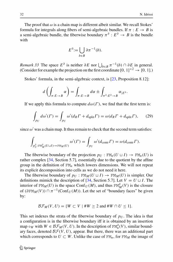
The proof that ω is a chain map is different albeit similar. We recall Stokes’formula for integrals along fibers of semi-algebraic bundles. If π : E → B isa semi-algebraic bundle, the fiberwise boundary π∂ : E∂ → B is the bundlewith

E∂ :=⋃

b∈B

∂π−1(b).

Remark 33 The space E∂ is neither ∂ E nor⋃

b∈B π−1(b) ∩ ∂ E in general.(Consider for example the projection on the first coordinate [0, 1]×2 → [0, 1].)

Stokes’ formula, in the semi-algebraic context, is [23, Proposition 8.12]:

d

(∫

π :E→Bα

)

=∫

π :E→Bdα ±

∫

π∂ :E∂→Bα|E∂ .

If we apply this formula to compute dω(Γ ), we find that the first term is:

∫

pU

dω′(Γ ) =∫

pU

ω′(dRΓ + dsplitΓ ) = ω(dRΓ + dsplitΓ ), (29)

sinceω′ was a chainmap. It thus remain to check that the second term satisfies:

∫

p∂U :FM∂

M (U�I )→FMM (U )

ω′(Γ ) =∫

pU

ω′(dcontrΓ ) = ω(dcontrΓ ).

The fiberwise boundary of the projection pU : FMn(U � I ) → FMn(U ) israther complex [34, Section 5.7], essentially due to the quotient by the affinegroup in the definition of FMn which lowers dimensions. We will not repeatits explicit decomposition into cells as we do not need it here.

The fiberwise boundary of pU : FMM(U � I ) → FMM(U ) is simpler. Ourdefinitions mimick the description of [34, Section 5.7]. Let V = U � I . Theinterior of FMM(U ) is the space ConfU (M), and thus FM∂

M(V ) is the closureof (∂FMM(V )) ∩ π−1(ConfU (M)). Let the set of “boundary faces” be givenby:

BFM(V, U ) = {W ⊂ V | #W ≥ 2 and #W ∩ U ≤ 1}.

This set indexes the strata of the fiberwise boundary of pU . The idea is thata configuration is in the fiberwise boundary iff it is obtained by an insertionmap ◦W with W ∈ BFM(V, U ). In the description of FM∂

n(V ), similar bound-ary faces, denoted BF(V, U ), appear. But there, there was an additional partwhich corresponds to U ⊂ W . Unlike the case of FMn , for FMM the image of

123


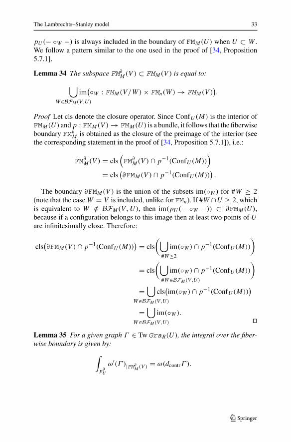
pU (− ◦W −) is always included in the boundary of FMM(U ) when U ⊂ W .We follow a pattern similar to the one used in the proof of [34, Proposition5.7.1].

Lemma 34 The subspace FM∂M(V ) ⊂ FMM(V ) is equal to:

⋃

W∈BFM (V,U )

im(◦W : FMM(V/W ) × FMn(W ) → FMM(V )

).

Proof Let cls denote the closure operator. Since ConfU (M) is the interior ofFMM(U ) and p : FMM(V ) → FMM(U ) is a bundle, it follows that the fiberwiseboundary FM∂

M is obtained as the closure of the preimage of the interior (seethe corresponding statement in the proof of [34, Proposition 5.7.1]), i.e.:

FM∂M(V ) = cls

(FM∂

M(V ) ∩ p−1(ConfU (M)))

= cls(∂FMM(V ) ∩ p−1(ConfU (M))

).

The boundary ∂FMM(V ) is the union of the subsets im(◦W ) for #W ≥ 2(note that the case W = V is included, unlike for FMn). If #W ∩U ≥ 2, whichis equivalent to W /∈ BFM(V, U ), then im(pU (− ◦W −)) ⊂ ∂FMM(U ),because if a configuration belongs to this image then at least two points of Uare infinitesimally close. Therefore:

cls(∂FMM(V ) ∩ p−1(ConfU (M))

) = cls

(⋃

#W≥2

im(◦W ) ∩ p−1(ConfU (M))

)

= cls

(⋃

#W∈BFM (V,U )

im(◦W ) ∩ p−1(ConfU (M))

)

=⋃

W∈BFM (V,U )

cls(im(◦W ) ∩ p−1(ConfU (M))

)

=⋃

W∈BFM (V,U )

im(◦W ).��

Lemma 35 For a given graph Γ ∈ TwGraR(U ), the integral over the fiber-wise boundary is given by:

∫

p∂U

ω′(Γ )|FM∂M (V ) = ω(dcontrΓ ).

123

34 N. Idrissi

Proof The maps ◦W : FMM(V/W ) × FMn(W ) → FMM(V ) are smoothinjective maps and their domains are compact, thus they are homeomor-phisms onto their images. Recall that #W ≥ 2 for W ∈ BFM(V, U ); hencedim FMn(W ) = n#W − n − 1. The dimension of the image of ◦W is then:

dim im(◦W ) = dim FMM(V/W ) + dim FMn(W )

= n#(V/W ) + (n#W − n − 1)

= n#V − 1,

i.e. the image is of codimension 1 in FMM(V ). It is also easy to check that ifW �= W ′, then im(◦W ) ∩ im(◦W ′) is of codimension strictly bigger than 1.

We now fix W ∈ BFM(V, U ). Since #W ∩ U ≤ 1, the composition U ⊂V → V/W is injective and identifies U with a subset of V/W . There is thena forgetful map p′

U : FMM(V/W ) → FMM(U ). We then have a commutativediagram:

FMM(V/W ) × FMn(W ) FMM(V/W )

FMM(V ) FMM(U )

◦W

p1

p′U

pU

. (30)

It follows that pU (− ◦W −) = p′U ◦ p1 is the composite of two semi-

algebraic bundles, hence it is a semi-algebraic bundle itself [23, Proposition8.5]. Combined with the fact about codimensions above, we can thereforeapply the summation formula [23, Proposition 8.11]:

∫

p∂U

ω′(Γ ) =∑

W∈BFM (V,U )

∫

pU (−◦W −)

ω′(Γ )|FMM (V/W )×FMn(W ). (31)

Nowwe can directly adapt the proof of Lambrechts andVolic. For a fixedW ,by [23, Proposition 8.13], the corresponding summand is equal to±ω(ΓV/W )·∫FMn(W )

ω′(ΓW ), where

– ΓV/W ∈ TwGraR(U ) is the graph with W collapsed to a vertex andU ↪→ V/W is identified with its image;

– ΓW ∈ TwGran(W ) is the full subgraph of Γ with vertices W and thelabels removed.

The vanishing lemmas in the proof of Lambrechts and Volic then imply thatthe integral

∫FMn(W )

ω′(ΓW ) is zero unless ΓW is the graph with exactly twovertices and one edge, in which case the integral is equal to 1. In this case,ΓV/W is the graph Γ with one edge connecting an internal vertex to someother vertex collapsed. The sum runs over all such edges, and dealing withsigns carefully we see that Eq. (31) is precisely equal to ω(dcontrΓ ). ��

123


We can now finish proving Proposition 32. We combine Eq. (29) andLemma 35, and apply Stokes’ formula to dω(Γ ) to show that it is equalto ω(dΓ ) = ω(dRΓ + dsplitΓ ) + ω(dcontrΓ ).

3.6 Reduced labeled graphs: GraphsR

The last step in the construction of GraphsR is the reduction of TwGraRso that it has the right cohomology. We borrow the terminology of Campos–Willwacher [6] for the next two definitions.

Definition 36 The full graph complex fGCR is the CDGA TwGraR(∅). Itconsists of labeled graphswith only internal vertices, and the product is disjointunion of graphs.

Remark 37 The adjective “full” refers to the fact that graphs are possiblydisconnected and have vertices of any valence in fGCR .

As an algebra, fGCR is free and generated by connected graphs. In gen-eral we will call internal components the connected components of a graphthat only contain internal vertices. The full graph complex naturally acts onTwGraR(U ) by adding extra internal components.

Definition 38 The partition function Zϕ : fGCR → R is the restriction ofω : TwGraR → Ω∗

PA(FMM) to fGCR = TwGraR(∅) → Ω∗PA(FMM(∅)) =

Ω∗PA(pt) = R.

Remark 39 The expression “partition function” comes from the mathematicalphysics literature, more specifically Chern–Simons invariant theory, where itrefers to the partition function of a quantum field theory.

By the double-pushforward formula [23, Proposition 8.13] and Fubini’stheorem [23, Proposition 8.15], Zϕ is an algebra morphism and

∀γ ∈ fGCR, ∀Γ ∈ TwGraR(U ), ω(γ · Γ ) = Zϕ(γ ) · ω(Γ ). (32)

Definition 40 Let Rϕ be the fGCR-module of dimension 1 induced by Zϕ :fGCR → R. The reduced graph comodule Graphsϕ

R is the tensor product:

GraphsϕR(U ):=Rϕ ⊗fGCR TwGraR(U ).

In other words, a graph of the type Γ � γ containing an internal componentγ ∈ fGCR is identified with Zϕ(γ ) ·Γ . It is spanned by representative classesof graphs with no internal connected component; we call such graphs reduced.The notation ismeant to evoke the fact thatGraphsϕ

R depends on the choice ofthe propagator ϕ, unlike the collection Graphsε

R that will appear in Sect. 4.1.

123

36 N. Idrissi

Proposition 41 The map ω : TwGraR(U ) → Ω∗PA(FMM(U )) defined in

Proposition 32 factors through the quotient defining GraphsϕR.

If χ(M) = 0, then GraphsϕR forms a Hopf right Graphsn-comodule.

If moreover M is framed, then the map ω defines a Hopf right comodulemorphism.

Proof Equation (32) immediately implies that ω factors through the quotient.The vanishing lemmas shows that if Γ ∈ TwGran(U ) has internal com-

ponents, then ω(Γ ) vanishes by [34, Lemma 9.3.7], so it is straightforwardto check that if χ(M) = 0, then Graphsϕ

R becomes a Hopf right comoduleover Graphsn . It is also clear that for M framed, the quotient map ω remainsa Hopf right comodule morphism. ��Proposition 42 ([7, Lemma 3]) The propagator ϕ can be chosen such thatthe following additional property (P4) holds:

∫

p1:FMM (2)→FMM (1)=Mp∗2(σ (x)) ∧ ϕ = 0, ∀x ∈ R. (P4)

From now on and until the end, we assume that ϕ satisfies (P4).

Remark 43 The additional property (P5) of the paper mentioned above wouldbe helpful in order to get a direct morphism Graphsϕ

R → GA, because thenthe partition function would vanish on all connected graphs with at least twovertices. However we run into difficulties when trying to adapt the proof inthe setting of PA forms, mainly due to the lack of an operator dM acting onΩ∗

PA(M × N ) differentiating “only in the first slot”.

Corollary 44 The morphism ω vanishes on graphs containing univalent inter-nal vertices.

Proof Let Γ ∈ GraR(U � I ) ⊂ TwGraR(U ) be a graph with a univalentinternal vertex u ∈ I , labeled by x , and let v be the only vertex connected to u.Let Γ be the full subgraph of Γ on the set of vertices U � I\{u}. Then using[23, Propositions 8.10 and 8.15] (in a way similar to the end of the proof of[34, Lemma 9.3.8]), we find:

ω(Γ ) =∫

FMM (U�I )→FMM (U )

ω′(Γ )

=∫

FMM (U�I )→FMM (U )

ω′(Γ )p∗uv(ϕ)p∗

u(σ (x))

=∫

FMM (U�I\{u})→FMM (U )

ω′(Γ )

∧ p∗v

(∫

FMM ({u,v})→FMM ({v})p∗

uv(ϕ)p∗u(σ (x))

)

,

123


which vanishes by (P4) in Proposition 42. ��Almost everything we have done so far works in full generality. We now

prove a fact which sets a class of manifolds apart.

Proposition 45 Assume that M is simply connected and that dim M ≥ 4. Thenthe partition function Zϕ vanishes on any connected graph with no bivalentvertices labeled by 1R and containing at least two vertices.

Remark 46 If γ ∈ fGCR has only one vertex, labeled by x , then Zϕ(γ ) =∫M σ(x) which can be nonzero.

Proof Let γ ∈ fGCR be a connected graph with at least two vertices and nobivalent vertices labeled by 1R . By Corollary 44, we can assume that all thevertices of γ are at least bivalent. By hypothesis, if a vertex is bivalent then itis labeled by an element of R>0 = R≥2.

Let k = i + j be the number of vertices of γ , with i vertices that are at leasttrivalent and j vertices that are bivalent and labeled by R≥2. It follows that γhas at least 1

2 (3i + 2 j) edges, all of degree n − 1. Since bivalent vertices arelabeled by R≥2, their labels contribute by at least 2 j to the degree of γ . The(internal) vertices contribute by −kn to the degree, and the other labels havea nonnegative contribution. Thus:

deg γ ≥(3

2i + j

)

(n − 1)+2 j −kn =(3

2k − 3

2j + j

)

(n − 1)+2 j − kn

= 1

2

(k(n − 3) − j (n − 5)

).

This last number is always positive for 0 ≤ j ≤ k: it is an affine functionof j , and it is positive when j = 0 and j = k (recall that n ≥ 4). Thedegree of γ ∈ fGCR must be zero for the integral defining Zϕ(γ ) to be theintegral of a top form of FMM(k) and hence possibly nonzero. But by the abovecomputation, deg γ > 0 �⇒ Zϕ(γ ) = 0. ��Remark 47 When n = 3, the manifold M is the 3-sphere S3 by Perelman’sproof of the Poincaré conjecture [41,42]. The partition function Zϕ is conjec-tured to be trivial on S3 for a proper choice of framing, thus bypassing theneed for the above degree counting argument. See also Proposition 80.

We will also need the following technical property of fGCR .

Lemma 48 The CDGA fGCR is cofibrant.

Proof We filter fGCR by the number of edges, defining FsfGCR to be thesubmodule of fGCR spanned by graphs of γ such that all the connected compo-nents γ have at most s edges. The differential of fGCR can only decrease (dsplit

123

38 N. Idrissi

and dcontr) or leave constant (dR) the number of edges. Moreover FsfGCR isclearly stable under products (disjoint unions), hence FsfGCR is a sub-CDGAof fGCR . It is also clear that fGCR = colims FsfGCR . We will prove thatF0fGCR is cofibrant, and that each FsfGCR ⊂ Fs+1fGCR is a cofibration.The CDGA F0fGCR is the free CDGA on graphs with a single vertex labeled

by R. In other words, F0fGCR = S(R, dR) is the free symmetric algebra onthe dg-module R, and any free symmetric algebra on a dg-module is cofibrant.

Let us now show that FsfGCR ⊂ Fs+1fGCR is a cofibration for any s ≥ 0.We will show that it is in fact a “relative Sullivan algebra” [13, Section 14].As a CDGA, we have Fs+1fGCR = (FsfGCR ⊗ S(Vs+1), d), where Vs+1 isthe graded module of connected graphs with exactly s + 1 edges. Let us nowshow the Sullivan condition.

Recall that R is obtained from the minimal model of M by a relative Sul-livan extension, hence it is itself a Sullivan algebra [13, Section 12]. In otherwords, R = (S(W ), d) where W is increasingly and exhaustively filtered byW (−1) = 0 ⊂ · · · ⊂ W (t) ⊂ · · · ⊂ W such that d(W (t)) ⊂ S(W (t − 1)).This induces a filtration on R by defining R(t):=⊕

t1+···+tr =t

(V (t1) ⊗ · · · ⊗

V (tr ))Σr.

This in turns induces an increasing and exhaustive filtration on Vs+1 bysubmodules Vs+1(t) as follows. A connected graph γ ∈ Vs+1 is in Vs+1(t)if each label xi ∈ R of a vertex of γ belongs to the filtration R(ti ) such that∑

ti = t . It is then immediate to check that d(Vs+1(t +1)) ⊂ Vs ⊗S(Vs+1(t)).Indeed, if γ ∈ Vs+1(t + 1), then dsplitγ and dcontrγ ∈ Vs , because bothstrictly decrease the number of edges. And dRγ ∈ Vs+1(t) because the internaldifferential of R decreases the filtration of R. ��

4 From the model to forms via graphs

In this section we connect GA to Ω∗PA(FMM) and we prove that the connecting

morphisms are quasi-isomorphisms. We assume that M is a simply connectedclosed smooth manifold with dim M ≥ 4 (see Proposition 45).

4.1 Construction of the morphism to GA

Proposition 49 For each finite set U, there is a CDGA morphism ρ′∗ :GraR(U ) → GA(U ) given by ρ on the R⊗U factor and sending the gen-erators euv to ωuv on the Gran factor. When χ(M) = 0, this defines a Hopfright comodule morphism (GraR,Gran) → (GA,e∨

n ). ��If we could find a propagator for which property (P5) held (see Remark 43),

then we could just send all graphs containing internal vertices to zero andobtain an extension Graphsϕ

R → GA. Since we cannot assume that (P5)

123


holds, the definition of the extension is more complex. However we still haveProposition 45, and homotopically speaking, graphs with bivalent vertices areirrelevant.

Definition 50 Let fGC0R be the quotient of fGCR defined by identifying a

disconnected vertex labeled by x with the number εA(ρ(x)).

Lemma 51 The subspace I ⊂ fGC0R spanned by graphs with at least one

univalent vertex, or at least one bivalent vertex labeled by 1R, or at least onelabel in ker(ρ : R → A), is a CDGA ideal.

Proof It is clear that I is an algebra ideal. Let us prove that it is a differentialideal. If one of the labels of Γ is in ker ρ, then so do all the summands of dΓ ,because ker ρ is a CDGA ideal of R.

IfΓ contains a bivalent vertex u labeled by 1R , then so does dRΓ . In dsplitΓ ,splitting one of the two edges connected to u produces a univalent vertex andhence vanishes in fGC0

R because the label is 1R . In dcontrΓ , the contraction ofthe two edges connected to u cancel each other.

Finally let us prove that if Γ has a univalent vertex u, then dΓ lies in I .It is clear that dRΓ ∈ I . Contracting or splitting the only edge connected tothe univalent vertex could remove the univalent vertex. Let us prove that thesetwo summands cancel each other up to ker ρ.

It is helpful to consider the case pictured in Eq. (28). Let y be thelabel of the univalent vertex u, and let x be the label of the only ver-tex incident to u. Contracting the edge yields a new vertex labeled byxy. Due to the definition of fGC0

R , splitting the edge yields a new ver-tex labeled by α:=∑

(ΔR) ε(ρ(xΔ′′R))yΔ′

R . We thus have ρ(α) = ρ(x) ·∑

(ΔA) ±εA(ρ(y)Δ′′A)Δ′

A.It is a standard property of the diagonal class that

∑(ΔA) ±εA(aΔ′′

A)Δ′A = a

for all a ∈ A (this property is a direct consequence of the definition in Eq. (21)).Applied to a = ρ(y), it follows from the previous equation that ρ(α) =±ρ(xy); examining the signs, this summand cancels from the summand thatcomes from contracting the edge. ��Definition 52 The algebra fGC′

R is the quotient of fGC0R by the ideal I .

Note that fGC′R is also free as an algebra,with generators given by connected

graphs with no isolated vertices, nor univalent vertices, nor bivalent verticeslabeled by 1R , and where the labels lie in R/ ker(ρ) = A.

Definition 53 A circular graph is a graph in the shape of a circle and whereall vertices are labeled by 1R , i.e. graphs of the type e12e23 . . . e(k−1)kek1.Let fLoopR ⊂ fGC0

R be the submodule spanned by graphs whose connectedcomponents either have univalent vertices or are equal to a circular graphs.

123

40 N. Idrissi

Lemma 54 The submodule fLoopR is a sub-CDGA of fGC0R.

Proof The submodule fLoopR is stable under products (disjoint union) bydefinition, so we just need to check that it is stable under the differential.Thanks to the proof of Lemma 51, in fGC0

R , if a graph contains a univalentvertex, then so do all the summands of its differential. On a circular graph, theinternal differential of R vanish, because all labels are equal to 1R . Contractingan edge in a circular graph yields another circular graph, and splitting an edgeyields a graph with univalent vertices, which belongs to fLoopR . ��Proposition 55 The sequence fLoopR → fGC0

R → fGC′R is a homotopy

cofiber sequence of CDGAs.

Proof The CDGA fGC0R is freely generated by connected labeled graphs with

at least two vertices. It is a quasi-free extension of fLoopR by the algebragenerated by graphs that are not circular and that do not contain any univalentvertices. The homotopy cofiber of the inclusion fLoopR → fGC0

R is thisalgebra fGC′′

R , generated by graphs that are not circular and do not containany univalent vertices, together with a differential induced by the quotientfGC0

R/(fLoopR).Let us note that the quotient map fGC0

R → fGC′R = fGC0

R/I vanishes onfLoopR , because fLoopR is included in R. Thus we have a diagram:

0 fLoopR fGC0R fGC′′

R :=fGC0R/fLoopR 0

0 I fGC0R fGC′

R :=fGC0R/I 0

Let us prove that themorphism fGC′′R → fGC′

R is a quasi-isomorphism.Definean increasing filtration on both algebras by letting FsfGC′

R (resp. FsfGC′′R) be

the submodule spanned by graphs Γ such that #edges − #vertices ≤ s. Thesplitting part of the differential strictly decreases the filtration, so only dR anddcontr remain on the first page of the associated spectral sequences.

One can then filter by the number of edges. On the first page of the spectralsequence associated to this new filtration, there is only the internal differentialdR . Thus on the second page, the vertices are labeled by H∗(R) = H∗(M).The contracting part of the differential decreases the new filtration by exactlyone, and so on the second page we see all of dcontr.

We can now adapt the proof of [53, Proposition 3.4] to show that on thepart of the complex with bivalent vertices, only the circular graphs contributeto the cohomology (we work dually so we consider a quotient instead of anideal, but the idea is the same). To adapt the proof, one must see the labelsof positive degree as formally adding one to the valence of the vertex, thus“breaking” a line of bivalent vertices. These labels break the symmetry (recall

123


the coinvariants in the definition of the twisting) that allow cohomology classesto be produced. ��Corollary 56 The morphism Zϕ : fGCR → R factors through fGC′

R in thehomotopy category of CDGAs.

Proof Let us show that Zϕ is homotopic to zero when restricted to the idealdefining fGC′

R = fGC0R/I as a quotient of fGCR . Up to rescaling εA by a real

coefficient, we may assume that εAρ(−) and∫

M σ(−) are homotopic, whichinduces a homotopy (by derivations) on the sub-CDGA of graphs with no edges.Hence Zϕ is homotopic to zerowhen restricted to the ideal defining fGC0

R fromfGCR . Moreover the map Zϕ vanishes on graphs with univalent vertices byCorollary 44. The degree of a circular graph with k vertices is −k < 0 (recallthat all the labels are 1R in a circular graph), but Zϕ vanishes on graphs ofnonzero degree. Hence Zϕ vanishes on the connected graphs appearing inthe definition of fLoopR . Therefore, in the homotopy category of CDGAs, Zϕ

factors through the homotopy cofiber of the inclusion fLoopR → fGC0R , which

is quasi-isomorphic to fGC′R by Proposition 55. ��

The statement of the corollary is not concrete, as the “factorization” couldgo through a zigzag of maps. However, the CDGAs fGCR and fGC′

R are bothcofibrant (see Lemma 48 for fGCR , whose proof can easily be adapted tofGC′

R). Recall from Sect. 1.1 the following definition of homotopy. Let π :fGCR → fGC′

R be the quotient map. Recall that A∗PL(Δ1) = S(t, dt) is a path

object for the CDGA R, and ev0, ev1 : A∗PL(Δ1) → R are evaluation at t = 0

and t = 1. There exists some morphism Z ′ϕ : fGC′

R → R and some homotopyh : fGCR → A∗

PL(Δ1) such that the following diagram commutes:

fGCR

R A∗PL(Δ1) R

Zϕ Z ′ϕπ

h

∼ev1 ev0

∼

Definition 57 Let A∗PL(Δ1)h be the fGCR-module induced by h, and let

Graphs′R(U ) = A∗

PL(Δ1)h ⊗fGCR TwGraR(U ).

Definition 58 Let Zε : fGCR → R be the algebra morphism that sends agraph γ with a single vertex labeled by x ∈ R to εA(ρ(x)), and that vanisheson all the other connected graphs.LetRε be the one-dimensional fGCR-moduleinduced by Zε, and let

GraphsεR(U ) = Rε ⊗fGCR TwGraR(U ).

123

42 N. Idrissi

Explicitly, in GraphsεR , all internal components with at least two vertices

are identified with zero, whereas an internal component with a single vertexlabeled by x ∈ R is identified with the number εA(ρ(x)).

Lemma 59 The morphism Z ′ϕπ is equal to Zε.

Proof This is a rephrasing of Proposition 45. Using the same degree countingargument, all the connected graphs with more than one vertex in fGC′

R areof positive degree. Since R is concentrated in degree zero, Z ′

ϕπ must vanishon these graphs, just like Zε. Moreover the morphism π : fGCR → fGC′

R =fGC0

R/I factors through fGC0R , where graphs γ with a single vertex are already

identified with the numbers Zε(γ ). ��Proposition 60 For each finite set U, we have a zigzag of quasi-isomorphismsof CDGAs:

GraphsεR(U )

∼←− Graphs′R(U )

∼−→ GraphsϕR(U ).

If χ(M) = 0, then Graphs′R and Graphsε

R are right Hopf Graphsn-comodules, and the zigzag defines a zigzag of Hopf right comodule morphisms.

Proof We have a commutative diagram:

GraphsεR(U ) Graphs′

R(U ) GraphsϕR(U )

TwGraR(U ) ⊗fGCR Rε TwGraR(U ) ⊗fGCR A∗PL(Δ1)h TwGraR(U ) ⊗fGCR Rϕ

= =1⊗ev1 1⊗ev0

=

The fGCR-module TwGraR(U ) is cofibrant. Indeed, it is quasi-free, becauseTwGraR(U ) is freely generated as a graded fGCR-module by reduced graphs.Moreover, we can adapt the proof of Lemma 48 to filter the space of generatorsin an appropriate manner and show that TwGraR(U ) is cofibrant.

Therefore the functor TwGraR(U ) ⊗fGCR (−) preserves quasi-isomorph-isms. The two evaluation maps ev0, ev1 : A∗

PL(Δ1) → R are quasi-isomorphisms. It follows that all the maps in the diagram are quasi-isomorphisms.

If χ(M) = 0, the proof that Graphs′R and Graphsε

R assemble toGraphsn-comodules is identical to the proof for Graphsϕ

R (see Proposi-tion 41). It is also clear that the two zigzags define morphisms of comodules:in Graphsn , as all internal components are identified with zero anyway. ��Proposition 61 The CDGA morphisms ρ′∗ : GraR(U ) → GA(U ) extend toCDGA morphisms ρ∗ : Graphsε

R(U ) → GA(U ) by sending all reduced graphscontaining internal vertices to zero. If χ(M) = 0 this extension defines a Hopfright comodule morphism.

123


Proof The submodule of reduced graphs containing internal vertices is a mul-tiplicative ideal and a cooperadic coideal, so all we are left to prove is thatρ∗ is compatible with differentials. Since ρ′∗ was a chain map, we must onlyprove that if Γ is a reduced graph with internal vertices, then ρ∗(dΓ ) = 0.

If a summand of dΓ still contains an internal vertex, then it is mapped tozero by definition ofρ∗. Sowe need to look for the summands of the differentialthat can remove all internal vertices at once.

The differential of R leaves the number of internal vertices constant, there-fore if Γ already had an internal vertex, so do all the summands of dRΓ . Thecontracting part dcontr of the differential decreases the number of internal ver-tices by exactly one, so let us assume that Γ has exactly one internal vertex.This vertex is at least univalent, as we consider reduced graphs. Then there areseveral cases to consider, depending of the valence of the internal vertex:

– if it is univalent, then the argument of Lemma 51 shows that contractingthe incident edge cancels with the splitting part of the differential;

– if it is bivalent, the contracting part has two summands, and both cancel bythe symmetry relation ιu(a)ωuv = ιv(a)ωuv in Eq. (22);

– if it is at least trivalent, then we can use the symmetry relation ιu(a)ωuv =ιv(a)ωuv to push all the labels on a single vertex, and we see that the sumof graphs that appear is obtained by the Arnold relation (see Fig. 1 for anexample in the case of Graphsn → e∨

n ).

Finally, the splitting part of the differential leaves the number of internalvertices constant, unless it splits off a whole connected component with onlyinternal vertices, in which case the component is evaluated using the partitionfunction Zε. If that connected component consists of a single internal ver-tex, then we saw in the previous item that splitting the edge connecting thisunivalent vertex to the rest of the graph cancels with the contraction of thatedge. Otherwise, if the graph has more than one vertex, then by definition Zε

vanishes on that graph. ��

4.2 The morphisms are quasi-isomorphisms

In this section we prove that the morphisms constructed in Proposition 41 andProposition 61 are quasi-isomorphisms, completing the proof of Theorem 3.

Let us recall our hypotheses and constructions. Let M be a simply connectedclosed smooth manifold of dimension at least 4. We endow M with a semi-algebraic structure (Sect. 1.3) and we consider the CDGA Ω∗

PA(M) of PA formson M , which is a model for the real homotopy type of M . Recall that we fix

a zigzag of quasi-isomorphisms of CDGAs Aρ←− R

σ−→ Ω∗PA(M), where A

is a Poincaré duality CDGA (Theorem 14), and σ factors through the quasi-isomorphic sub-CDGA of trivial forms.

123

44 N. Idrissi

Recall that ϕ ∈ Ωn−1PA (FMM(2)) is an (anti-)symmetric trivial form on

the compactification of the configuration space of two points in M , whoserestriction to the sphere bundle ∂FMM(2) is a global angular form, and whosedifferential dϕ is a representative of the diagonal class of M (Proposition 25).Recall that we defined the graph complexGraphsϕ

R(U ) using reduced labeledgraphs with internal and external vertices (Definition 40) and a partition func-tion built from ϕ (Definition 38). We also defined the variants Graphsε

R andGraphs′

R (Definitions 57 and 58).

Theorem 62 (Precise version of Theorem 3) Let M be a simply connectedclosed smooth manifold of dimension at least 4. Using the notation recalledabove, the following zigzag, where the maps were constructed in Proposi-tion 41, Proposition 60, and Proposition 61, is a zigzag of quasi-isomorphismsof Z-graded CDGAs for all finite sets U:

GA(U )∼←− Graphsε

R(U )∼←− Graphs′

R(U )∼−→ Graphsϕ

R(U )∼−→ Ω∗

PA(FMM (U )).

If χ(M) = 0, then the left-pointing maps form a quasi-isomorphism of Hopfright comodules:

(GA,e∨n )

∼←− (GraphsεR,Graphsn)

∼←− (Graphs′R,Graphsn).

If moreover M is framed, then the right-pointing maps also form a quasi-isomorphism of Hopf right comodules:

(Graphs′R,Graphsn)

∼−→ (GraphsϕR,Graphsn)

∼−→ (Ω∗PA(FMM ), Ω∗

PA(FMn)).

The rest of the section is dedicated to the proof of this theorem. Let us give aroadmap of this proof. We first prove that Graphsε

R(U ) → GA(U ) is a quasi-isomorphism by an inductive argument on #U (Proposition 64). This involvessetting up a spectral sequence so that we can reduce the argument to connectedgraphs. Then we use explicit homotopies in order to show that both complexeshave cohomology of the same dimension, and we show that the morphism issurjective on cohomology by describing a section by explicit arguments. Thenwe prove that Graphsϕ

R(U ) → Ω∗PA(FMM(U )) is surjective on cohomology

explicitly (Proposition 76). Since we know that GA(U ) and FMM(U ) have thesame cohomology by the theorem of Lambrechts–Stanley [33, Theorem 10.1],this completes the proof that all the maps are quasi-isomorphisms. Compati-bility with the various comodules structures was already shown in Sect. 3.

Lemma 63 The morphisms GraphsεR(U ) → GA(U ) factor through quasi-

isomorphisms GraphsεR(U ) → Graphsε

A(U ), where GraphsεA(U ) is the

CDGA obtained by modding graphs with a label in ker(ρ : R → A) inGraphsε

R(U ).

123


Proof The morphism GraphsεR → Graphsε

A simply applies the surjectivemap ρ : R → A to all the labels. Hence Graphsε

R → GA factors through thequotient.

We can consider the spectral sequences associated to the filtrations of bothGraphsε

R and GraphsεA by the number of edges, and we obtain a mor-

phism E0GraphsεR → E0Graphsε

A. On both E0 pages, only the internaldifferentials coming from R and A remain. The chain map R → A is a quasi-isomorphism; hence we obtain an isomorphism on the E1 page. By standardspectral sequence arguments, it follows that Graphsε

R → GraphsεA is a

quasi-isomorphism. ��The CDGA Graphsε

A(U ) has the same graphical description as the CDGA

GraphsεR(U ), except that now vertices are labeled by elements of A. An

internal component with a single vertex labeled by a ∈ A is identified withε(a), and an internal component with more than one vertex is identified withzero.

Proposition 64 The morphism GraphsεA → GA is a quasi-isomorphism.

Before starting to prove this proposition, let us outline the different steps.We filter our complex in such a way that on the E0 page, only the contractingpart of the differential remains (such a technique was already used in the proofof Proposition 55). Using a splitting result, we can focus on connected graphs.Finally, we use a “trick” (Fig. 2) for moving labels around in a connectedcomponent, reducing ourselves to the case where only one vertex is labeled.We then get a chain map A ⊗ Graphsn → A ⊗ e∨

n (U ), which is a quasi-isomorphism thanks to the formality theorem.

Let us start with the first part of the outlined program, removing the splittingpart of the differential from the picture. We now define an increasing filtrationon Graphsε

A. The submodule FsGraphsεA is spanned by reduced graphs

such that #edges − #vertices ≤ s.

Lemma 65 The above submodules define a filtration of GraphsεA by sub-

complexes, satisfying F−#U−1GraphsεA(U ) = 0 for each finite set U. The E0

page of the spectral sequence associated to this filtration is isomorphic as amodule to Graphsε

A. Under this isomorphism the differential d0 is equal todA + d ′

contr, where dA is the internal differential coming from A and d ′contr is

the part of the differential that contracts all edges but edges connected to aunivalent internal vertex.

Proof Let Γ be an internally connected (Definition 11) reduced graph. IfΓ ∈ Graphsε

A(U ) is the graph with no edges and no internal vertices, thenit lives in filtration level −#U . Adding edges can only increase the filtration.Since we consider reduced graphs (i.e. no internal components), each time we

123

46 N. Idrissi

add an internal vertex (decreasing the filtration) we must add at least one edge(bringing it back up). By induction on the number of internal vertices, eachgraph is of filtration at least −#U .

Let us nowprove that the differential preserves the filtration and checkwhichparts remain on the associated graded complex. The internal differential dAdoes not change either the number of edges nor the number of vertices andso keeps the filtration constant. The contracting part dcontr of the differentialdecreases both by exactly one, and so keeps the filtration constant too.

The splitting part dsplit of the differential removes one edge. If the resultinggraph is still connected, then nothing else changes and thefiltration is decreasedexactly by 1. If the resulting graph is not connected, then we get an internalcomponent γ which was connected to the rest of the graph by a single edge,and was then split off and identified with a number in the process. If γ hasa single vertex labeled by a (i.e. we split an edge connected to a univalentvertex), then this number is ε(a), and the filtration is kept constant. Otherwise,the summand is zero (and so the filtration is obviously preserved).

In all cases, the differential preserves the filtration, and so we get a filteredchain complex. On the associated graded complex, the only remaining partsof the differential are dA, dcontr, and the part that splits off edges connected tounivalent vertices. But by the proof of Proposition 61 this last part cancels outwith the part that contracts these edges connected to univalent vertices. ��

The symmetric algebra S(ωuv)u �=v∈U has a weight grading by the word-length on the generatorsωuv. This induces aweight grading one∨

n (U ), becausethe ideal defining the relations is compatible with the weight grading. Thisgrading in turn induces an increasing filtration F ′

sGA on GA (the extra differ-ential strictly decreases the weight). Define a shifted filtration on GA by:

FsGA(U ):=F ′s+#UGA(U ).

Lemma 66 The E0 page of the spectral sequence associated to F∗GA is iso-morphic as a module to GA. Under this isomorphism the d0 differential is justthe internal differential of A. ��Lemma 67 The morphism Graphsε

A → GA preserves the filtration andinduces a chain map E0Graphsε

A(U ) → E0GA(U ), for each U. It mapsreduced graphs with internal vertices to zero, an edge euv between externalvertices to ωuv, and a label a of an external vertex u to ιu(a).

Proof The morphism GraphsεA(U ) → GA(U ) preserves the filtration by

construction. If a graph has internal vertices, then its image in GA(U ) is ofstrictly lower filtration unless the graph is a forest (i.e. a product of trees).But trees have leaves, therefore by Corollary 44 and the formula defining

123


GraphsεA → GA they are mapped to zero in GA(U ) anyway. It is clear that

the rest of the morphism preserves filtrations exactly, and so is given on theassociated graded complex as stated in the lemma. ��

We now use arguments similar to [34, Lemma 8.3]. For a partition π of U ,define the submodule Graphsε

A〈π〉 ⊂ E0GraphsεA(U ) spanned by reduced

graphs Γ such that the partition ofU induced by the connected components ofΓ is exactlyπ . In particular letGraphsε

A〈{U }〉 be the submodule of connectedgraphs,where {U } is the indiscrete partition ofU consisting of a single element.

Lemma 68 For each partition π of U, GraphsεA〈π〉 is a subcomplex of

E0GraphsεA(U ), and E0Graphsε

A(U ) splits as the sum over all partitionsπ :

E0GraphsεA(U ) =

⊕

π

⊗

V ∈π

GraphsεA〈{V }〉.

Proof Since there is no longer any part of the differential that can split offconnected components in E0Graphsε

A, it is clear that GraphsεA〈{U }〉 is a

subcomplex. The splitting result is immediate. ��The complex E0GA(U ) splits in a similar fashion. For a monomial in

S(ωuv)u �=v∈U , say that u and v are “connected” if the term ωuv appears inthe monomial. Consider the equivalence relation generated by “u and v areconnected”. The monomial induces in this way a partition π of U , and thisdefinition factors through the quotient defining e∨

n (U ) (draw a picture of the3-term relation). Finally, for a givenmonomial in GA(U ), the induced partitionof U is still well-defined.

Thus for a given partition π of U , we can define e∨n 〈π〉 and GA〈π〉 to be

the submodules of e∨n (U ) and E0GA(U ) spanned by monomials inducing the

partition π . It is a standard fact that e∨n 〈{U }〉 = Lie∨

n (U ), see [47]. The proofof the following lemma is similar to the proof of the previous lemma:

Lemma 69 For each partition π of U, GA〈π〉 is a subcomplex of E0GA(U ),and E0GA(U ) splits as the sum over all partitions π of U:

E0GA(U ) =⊕

π

⊗

V ∈π

GA〈{V }〉.

��Lemma 70 The map E0Graphsε

A(U ) → E0GA(U ) preserves the splitting.

We can now focus on connected graphs to prove Proposition 64.

Lemma 71 The complex GA〈{U }〉 is isomorphic to A ⊗ e∨n 〈{U }〉.

123

48 N. Idrissi

Proof We define explicit isomorphisms in both directions.Define A⊗U ⊗ e∨

n 〈{U }〉 → A ⊗ e∨n 〈{U }〉 using the multiplication of A.

This constructions induces a map on the quotient E0GA(U ) → A ⊗e∨n 〈{U }〉,

which restricts to a map GA〈{U }〉 → e∨n 〈{U }〉. Since dA is a derivation, this

is a chain map.Conversely, define A⊗e∨

n 〈{U }〉 → A⊗U ⊗e∨n 〈{U }〉 by a ⊗ x �→ ιu(a)⊗ x

for some fixed u ∈ U (it does not matter which one since x ∈ e∨n 〈{U }〉 is

“connected”). This construction gives a map A ⊗ e∨n 〈{U }〉 → GA〈{U }〉, and

it is straightforward to check that this map is the inverse isomorphism of theprevious map. ��

We have a commutative diagram of complexes:

GraphsεA〈{U }〉 A ⊗ Graphs′

n〈{U }〉

GA〈{U }〉 A ⊗ e∨n 〈{U }〉∼

∼=

Here Graphs′n(U ) is defined similarly to Graphsn(U ) except that mul-

tiple edges are allowed. It is known that the quotient map Graphs′n(U ) →

e∨n (U ) (which factors through Graphsn(U )) is a quasi-isomorphism [53,

Proposition 3.9]. The subcomplex Graphs′n〈{U }〉 is spanned by connected

graphs. The upper horizontal map in the diagram multiplies all the labels of agraph.

The right vertical map is the tensor product of idA and Graphsn〈{U }〉 ∼−→e∨

n 〈{U }〉 (see 1.6). The bottom row is the isomorphism of the previous lemma.It then remains to prove that Graphsε

A〈{U }〉 → A ⊗ Graphs′n〈{U }〉 is a

quasi-isomorphism to prove Proposition 64. If U = ∅, then Graphs′A(∅) =

R = GA(∅) and the morphism is the identity, so there is nothing to do. Fromnow on we assume that #U ≥ 1.

Lemma 72 The morphism GraphsεA〈{U }〉 → A ⊗ Graphs′

n〈{U }〉 is sur-jective on cohomology.

Proof Choose some u ∈ U . There is an explicit chain-level section of themorphism, sending x ⊗ Γ to Γu,x , the same graph with the vertex u labeledby x and all the other vertices labeled by 1R . It is a well-defined chain map,which is clearly a section of the morphism in the lemma, hence the morphismof the lemma is surjective on cohomology. ��

We now use a proof technique similar to the proof of [34, Lemma 8.3],working by induction. The dimension of H∗(Graphs′

n〈{U }〉) = e∨n 〈{U }〉 =

Lie∨n (U ) is well-known:

123


dim Hi (Graphs′n〈{U }〉) =

{(#U − 1)!, if i = (n − 1)(#U − 1);0, otherwise.

(33)

Lemma 73 For all sets U with#U ≥ 1, the dimension of Hi (GraphsεA〈{U }〉)

is the same as the dimension:

dim Hi (A ⊗ Graphs′n〈{U }〉) = (#U − 1)! · dim Hi−(n−1)(#U−1)(A).

The proof will be by induction on the cardinality of U . Before proving thislemma, we will need two additional sub-lemmas.

Lemma 74 The complex GraphsεA〈1〉 has the same cohomology as A.

Proof Let I be the subcomplex spanned by graphs with at least one internalvertex.We will show that I is acyclic; as Graphsε

A〈1〉/I ∼= A, this will provethe lemma.

There is an explicit homotopy h that shows that I is acyclic. Given a graphΓ with a single external vertex and at least one internal vertex, define h(Γ )

to be the same graph with the external vertex replaced by an internal vertex, anew external vertex labeled by 1A, and an edge connecting the external vertexto the new internal vertex:

ux h�−→ u

1A x

The differential in GraphsεA〈1〉 only retains the internal differential of A and

the contracting part of the differential. Contracting the new edge in h(Γ ) givesΓ back, and it is now straightforward to check that dh(Γ ) = Γ ± h(dΓ ). ��

Now let U be a set with at least two elements, and fix some element u ∈ U .LetGraphsu

A〈{U }〉 ⊂ GraphsεA〈{U }〉 be the subcomplex spanned by graphs

Γ such that u has valence 1, is labeled by 1A, and is connected to anotherexternal vertex.

We now get to the core of the proof of Lemma 73. The idea (adapted from[34, Lemma 8.3]) is to “push” the labels of positive degree away from thechosen vertex u through a homotopy. Roughly speaking, we use Fig. 2 tomove labels around up to homotopy.

Lemma 75 The inclusion GraphsuA〈{U }〉 ⊂ Graphsε

A〈{U }〉 is a quasi-isomorphism.

123

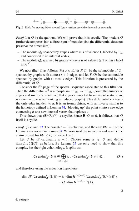
50 N. Idrissi

d contrx

=x

−x

Fig. 2 Trick for moving labels around (gray vertices are either internal or external)

Proof Let Q be the quotient. We will prove that it is acyclic. The module Qfurther decomposes into a direct sum of modules (but the differential does notpreserve the direct sum):

– The moduleQ1 spanned by graphs where u is of valence 1, labeled by 1A,and connected to an internal vertex;

– The moduleQ2 spanned by graphs where u is of valence≥ 2 or has a labelin A>0.

We now filter Q as follows. For s ∈ Z, let FsQ1 be the submodule of Q1spanned by graphs with at most s + 1 edges, and let FsQ2 be the submodulespanned by graphs with at most s edges. This filtration is preserved by thedifferential of Q.

Consider the E0 page of the spectral sequence associated to this filtration.Then the differential d0 is a morphism E0Q1 → E0Q2 (count the number ofedges and use the crucial fact that edges connected to univalent vertices arenot contractible when looking at reduced graphs). This differential contractsthe only edge incident to u. It is an isomorphism, with an inverse similar tothe homotopy defined in Lemma 74, “blowing up” the point u into a new edgeconnecting u to a new internal vertex that replaces u.

This shows that (E0Q, d0) is acyclic, hence E1Q = 0. It follows that Qitself is acyclic. ��Proof of Lemma 73 The case #U = 0 is obvious, and the case #U = 1 of thelemma was covered in Lemma 74. We now work by induction and assume theclaim proved for #U ≤ k, for some k ≥ 1.

Let U be of cardinality k + 1. Choose some u ∈ U and defineGraphsu

A〈{U }〉 as before. By Lemma 75 we only need to show that thiscomplex has the right cohomology. It splits as:

GraphsuA〈{U }〉 ∼=

⊕

v∈U\{u}euv · Graphsε

A〈{U\{u}}〉, (34)

and therefore using the induction hypothesis:

dim Hi (GraphsuA〈{U }〉) = k · dim Hi−(n−1)(Graphsε

A〈{U\{u}}〉)= k! · dim Hi−k(n−1)(A).

��

123


Proof of Proposition 64 By Lemma 72, the morphism induced by GraphsεA

→ GA on theE0 page is surjective on cohomology. By Lemma 73 and Eq. (33),both E0 pages have the same cohomology, and so the induced morphism is aquasi-isomorphism. Standard spectral arguments imply the proposition. ��Proposition 76 The morphism ω : Graphs′

R(U ) → Ω∗PA(FMM(U )) is a

quasi-isomorphism.

Proof ByEq. (23), Proposition 60, Lemma63, andProposition 64, both CDGAshave the same cohomology of finite type, so it will suffice to show that themap is surjective on cohomology to prove that it is a quasi-isomorphism.

We work by induction. The caseU = ∅ is immediate, as Graphs′R(∅)

∼−→Graphsϕ

R(∅) = Ω∗PA(FMM(∅)) = R and the last map is the identity.

Suppose that U = {u} is a singleton. Since ρ is a quasi-isomorphism,for every cocycle α ∈ Ω∗

PA(FMM(U )) = Ω∗PA(M) there is some cocycle

x ∈ R such that ρ(x) is cohomologous to α. Then the graph γx with a single(external) vertex labeled by x is a cocycle in Graphs′

R(U ), and ω(γx ) =ρ(x) is cohomologous to α. This proves that Graphs′

R({u}) → Ω∗PA(M) is

surjective on cohomology, and hence is a quasi-isomorphism.Now assume that U = {u} � V , where #V ≥ 1, and assume that the claim

is proven for sets of vertices of size at most #V = #U − 1. By Eq. (23), wemay represent any cohomology class of FMM(U ) by an element z ∈ GA(U )

satisfying dz = 0. Using the relations defining GA(U ), we may write z as

z = z′ +∑

v∈V

ωuvzv,

where z′ ∈ A ⊗GA(V ) and zv ∈ GA(V ). The relation dz = 0 is equivalent to

dz′ +∑

v∈V

(pu × pv)∗(ΔA) · zv = 0, (35)

and dzv = 0 for all v. (36)

By the induction hypothesis, for all v ∈ V there exists a cocycle γv ∈Graphs′

R(V ) such thatω(γv) represents the cohomology class of the cocyclezv in H∗(FMM(V )), and such that σ∗(γv) is equal to zv up to a coboundary.

By Eq. (35), the cocycle

γ =∑

v∈V

(pu × pv)∗(ΔR) · γv ∈ R ⊗ Graphs′

R(V )

is mapped to a coboundary in A⊗GA(V ). Themap σ∗ : R⊗Graphs′R(V ) →

A ⊗ GA(V ) is a quasi-isomorphism, hence γ = dγ1 is a coboundary too.

123

52 N. Idrissi

It follows that z′ −σ∗(γ1) ∈ A ⊗GA(V ) is a cocycle. Thus by the inductionhypothesis there exists some γ2 ∈ R⊗Graphs′

R(V )whose cohomology classrepresents the same cohomology class as z′ − σ∗(γ1) in H∗(A ⊗ GA(V )) =H∗(M × FMM(V )).We now let γ ′ = −γ1 + γ2, hence dγ ′ = −γ + 0 = −γ and σ∗(γ ′) is

equal to z′ up to a coboundary. By abuse of notation we still let γ ′ be theimage of γ ′ under the obvious map R ⊗ Graphs′

R(V ) → Graphs′R(U ),

x ⊗ Γ �→ ιu(x) · Γ . Then

γ = γ ′ +∑

v∈V

euv · γv ∈ Graphs′R(U )

is a cocycle, andω(γ ) represents the cohomology class of z inΩ∗PA(FMM(U )).

We have shown that the morphism Graphs′R(U ) → Ω∗

PA(FMM(U )) is sur-jective on cohomology, and hence it is a quasi-isomorphism. ��Proof of Theorem 62 The zigzag of the theorem becomes, after factorizing thefirst map through Graphsε

A:

GA(U ) ← GraphsεA(U ) ← Graphsε

R(U ) ←Graphs′

R(U ) → GraphsϕR(U ) → Ω∗

PA(FMM(U ))

All these maps are quasi-isomorphisms by Lemma 63, Proposition 60,Proposition 64, and Proposition76. Their compatibility with the comodulestructures (under the relevant hypotheses) are due to Proposition 41, Proposi-tion 60, and Proposition 61. ��

The last thing we need to check is the following proposition, which showsthat that we can choose any Poincaré duality model.

Proposition 77 If A and A′ are two quasi-isomorphic simply connectedPoincaré duality CDGAs, then there is a weak equivalence of symmetric collec-tions GA � GA′ . If moreover χ(A) = 0 then this weak equivalence is a weakequivalence of right Hopf e∨

n -comodules.

Proof The CDGAs A and A′ are quasi-isomorphic, hence there exists somecofibrant S and quasi-isomorphisms f : S

∼−→ A and f ′ : S∼−→ A′. This yields

two chain maps ε = εA ◦ f, ε′ = εA′ ◦ f ′ : S → R[−n]. Mimicking the proofof Proposition 15, we can also find (anti-)symmetric cocycles Δ, Δ′ ∈ S ⊗ Sand such that ( f ⊗ f )Δ = ΔA and ( f ′ ⊗ f ′)Δ′ = ΔA′ .

We can then build symmetric collections Graphsε,ΔS and a quasi-

isomorphism f∗ : Graphsε,ΔS → GA similarly to Sect. 3. The differential

of an edge euv in Graphsε,ΔS is ιuv(Δ), and an isolated internal vertex labeled

123


by x ∈ S is identifiedwith ε(x). In parallel, we can build f ′∗ : Graphsε′,Δ′S

∼−→GA′ .

If moreover χ(A) = 0, then we can choose Δ, Δ′ such that both graphcomplexes become right Hopf Graphsn-comodules, and f∗, f ′∗ are compat-ible with the comodule structure. It thus suffices to find a quasi-isomorphismGraphsε,Δ

S � Graphsε′,Δ′S to prove the proposition.

We first have an isomorphism Graphsε′,Δ′S

∼= Graphsε′,ΔS (with the obvi-

ous notation). Indeed, the two cocycles Δ and Δ′ are cohomologous, sayΔ′ − Δ = dα for some α ∈ S ⊗ S of degree n − 1. If we replace α by(α + (−1)nα21)/2, then we can assume that α21 = (−1)nα. Moreover ifχ(A) = 0, then we can replace α by α − (μS(α) ⊗ 1 + (−1)n1 ⊗ μS(α))/2to get μS(α) = 0. We then obtain an isomorphism by mapping an edge euv toeuv ± ιuv(α) (the sign depending on the direction of the isomorphism). Thismap is compatible with differentials, with products, and with the comodulestructures if χ(A) = 0.

The dg-module S is cofibrant andR[−n] is fibrant (like all dg-modules).Wecan assume that ε and ε′ induce the same map on cohomology (it suffices torescale one map, say ε′, and there is an automorphism of Graphsε′,Δ

S whichtakes care of this rescaling). Thus the two maps ε, ε′ : S → R[−n] are homo-topic, i.e. there exists some h : S[1] → R[−n] such that ε(x)−ε′(x) = h(dx)

for all x ∈ S. This homotopy induces a homotopy between the two morphismsZε, Zε′ : fGCS → R. Because TwGraΔ

S (U ) and TwGraΔ′S (U ) are cofi-

brant as modules over fGCS , we obtain quasi-isomorphisms Graphsε,ΔS �

Graphsε′,ΔS (compare with Proposition 60). ��

Corollary 78 Let M be a smooth simply connected closed manifold and A beany Poincaré duality model of M. Then GA(k) is a real model for Confk(M).

Proof The corollary follows from Theorem 62 in the case where dim M ≥4 (together with the previous proposition to ensure that we can choose anyPoincaré duality model A in our constructions). Note that the graph complexesare, in general, nonzero even in negative degrees, but by Proposition 4 this doesnot change the result. In dimension at most 3, the only examples of simplyconnected closed manifolds are S2 and S3. We address these examples inSect. 4.3. ��Corollary 79 The real homotopy types of the configuration spaces of a smoothsimply connected closed manifold only depends on the real homotopy type ofthe manifold.

Proof When dim M ≥ 3, the Fadell–Neuwirth fibrations [12] Confk−1(M\∗)

↪→ Confk(M) → M show by induction that if M is simply connected, then

123

54 N. Idrissi

so is Confk(M) for all k ≥ 1. Hence the real model GA(k) completely encodesthe real homotopy type of Confk(M). ��

4.3 Models for configurations on the 2- and 3-spheres

The degree-counting argument of Proposition 45 does not work in dimensionless than 4, sowe have to use othermeans to prove that the Lambrechts–StanleyCDGAs are models for the configuration spaces.

There are no simply connected closed manifolds of dimension 1. In dimen-sion 2, the only simply connected closed manifold is the 2-sphere, S2. Thismanifold is a complex projective variety: S2 = CP

1. Hence the result ofKriz [30] shows that GH∗(S2)(k) (denoted E(k) there) is a rational model forConfk(S2). The 2-sphere S2 is studied in greater detail in Sect. 6, where westudy the action of the framed little 2-disks operad on a framed version ofFMS2 .

In dimension 3, the only simply connected smooth closed manifold is the3-sphere by Perelman’s proof of the Poincaré conjecture [41,42]. we also thefollowing partial result, communicated to us by Thomas Willwacher:

Proposition 80 The CDGA GA(k), where A = H∗(S3; Q), is a rational modelof Confk(S3) for all k ≥ 0.

Proof The claim is clear for k = 0. Since S3 is a Lie group, the Fadell–Neuwirth fibration is trivial [12, Theorem 4]:

Confk(R3) ↪→ Confk+1(S3) → S3

The space Confk+1(S3) is thus identified with S3 × Confk(R3), which is

rationally formal with cohomology H∗(S3) ⊗ e∨3 (k). It thus suffices to build

a quasi-isomorphism between GA(k + 1) and H∗(S3) ⊗ e∨n (k).

To simplify notation, we consider GA(k+) (where k+ = {0, . . . , k}), whichis obviously isomorphic to GA(k + 1). Let us denote by υ ∈ H3(S3) = A3

the volume form of S3, and recall that the diagonal class ΔA is given by1 ⊗ υ − υ ⊗ 1. We have an explicit map f : H∗(S3) → e∨

3 (k) given ongenerators by f (ν ⊗ 1) = ι0(ν) and f (1 ⊗ ωi j ) = ωi j + ω0i − ω0 j .

The Arnold relations show that this is a well-defined algebra morphism. Letus prove that d ◦ f = 0 on the generator ωi j (the vanishing on υ ⊗ 1 is clear).We may assume that k = 2 and (i, j) = (1, 2), and then apply ιi j to get thegeneral case. Then we have:

(d ◦ f )(ω12) = (1 ⊗ 1 ⊗ υ − 1 ⊗ υ ⊗ 1) + (1 ⊗ υ ⊗ 1 − υ ⊗ 1 ⊗ 1)

−(1 ⊗ 1 ⊗ υ − υ ⊗ 1 ⊗ 1) = 0

123


We know that both CDGAs have the same cohomology, so to check that fis a quasi-isomorphism it suffices to check that it is surjective in cohomology.The cohomology H∗(GA(k+)) ∼= H∗(S3) ⊗ e∨

3 (k) is generated in degrees 2(by the ωi j ’s) and 3 (by the ιi (υ)’s), so it suffices to check surjectivity in thesedegrees.

In degree 3, the cocycle υ ⊗ 1 is sent to a generator of H3(GA(k+)) ∼=H3(S3) = Q. Indeed, assume ι0(υ) = dω, where ω is a linear combinationof the ωi j for degree reasons. In dω, the sum of the coefficients of each ιi (υ)

is zero, because they all come in pairs (dωi j = ι j (υ) − ιi (υ)). We want thecoefficient of ι0(υ) to be 1, so at least one of the other coefficient must benonzero to compensate, hence dω �= ι0(υ).

It remains to prove that H2( f ) is surjective. We consider the quotient mapp : GA(k+) → e∨

3 (k) that maps ιi (υ) and ω0i to zero for all 1 ≤ i ≤ k. Wealso consider the quotient map q : H∗(S3) ⊗ e∨

3 (k) → e∨3 (k) sending υ ⊗ 1

to zero. We get a morphism of short exact sequences:

0 ker q H∗(S3) ⊗ e∨3 (k) e∨

3 (k) 0

0 ker p GA(k) e∨3 (k) 0

q

f =p

We consider part of the long exact sequence in cohomology induced bythese short exact sequences of complexes:

e∨3 (k)1 H2(ker q) H2(H∗(S3) ⊗ e∨

3 (k)) = e∨3 (k)2 e∨

3 (k)2

e∨3 (k)1 H2(ker p) H2(GA(k+)) e∨

3 (k)2= (1) H2( f ) =

For degree reasons, H2(ker q) = 0 and so the map (1) is injective. Bythe four lemma, it follows that H2( f ) is injective. Since both domain andcodomain have the same finite dimension, it follows that H2( f ) is an isomor-phism. ��

5 Factorization homology of universal enveloping En-algebras

5.1 Factorization homology and formality

The manifold Rn is framed. Let U be a finite set and consider the space of

framed embeddings (i.e. such that the differential at each point preserves thegiven trivializations of the tangent bundles) of U copies of R

n in itself, withthe compact open topology:

123

56 N. Idrissi

Diskfrn (U ) := Embfr(Rn × U, Rn) ⊂ Map(Rn × U, R

n). (37)

Using composition of embeddings, these spaces assemble to form a topo-logical operad Diskfrn . This operad is weakly equivalent to the operad of littlen-disks [3, Remark 2.10], and the application that takes f ∈ Diskfrn (U ) to{ f (0 × u)}u∈U ∈ ConfU (Rn) is a homotopy equivalence.

Similarly if M is a framed manifold, then the spaces Embfr(Rn × −, M)

assemble to form a topological right Diskfrn -module, again given by composi-tion of embeddings. We call it DiskfrM . If B is a Diskfrn -algebra, factorizationhomology is given by a derived composition product [3, Definition 3.2]:

∫

MB := DiskfrM ◦L

DiskfrnB:=

hocoeq(DiskfrM ◦ Diskfrn ◦ B ⇒ DiskfrM ◦ B

). (38)

Using [52, Section 2], the pair (FMM ,FMn) is weakly equivalent to the pair(DiskfrM ,Diskfrn ). So if B is an FMn-algebra, then its factorization homologyis:

∫

MB � FMM ◦L

FMnB:= hocoeq

(FMM ◦ FMn ◦ B ⇒ FMM ◦ B

). (39)

We nowwork in the category of chain complexes overR.We use the formal-ity theorem (Sect. 1.6) and the fact that weak equivalences of operads induceQuillen equivalence between categories of right modules (resp. categories ofalgebras) by [16, Theorems 16.A, 16.B]. Thus, to any homotopy class [B] ofEn-algebras in the category of chain complexes, there corresponds a homotopyclass [B] of en-algebras (which is generally not easy to describe).

UsingTheorem62, a gameof adjunctions [16, Theorems 15.1.A and 15.2.A]shows that:

∫

MB � G∨

A ◦L

enB, (40)

where A is the Poincaré duality model of M mentioned in the theorem, andG∨

A is the right en-module dual to GA viewed as a chain complex.

5.2 Higher enveloping algebras

Knudsen [27, Theorem A] considers a higher enveloping algebra functor UnfromhomotopyLie algebras to nonunital En-algebras. This functor generalizesthe standard enveloping algebra functor from the category of Lie algebras tothe category of associative algebras.

123


Let n be at least 2. We can again use Kontsevich’s theorem on the formalityof the little disks operads to identity the category of non-unital En-algebraswith the category of en-algebras in homotopy. We also use that a homotopyLie algebra is equivalent, in homotopy, to an ordinary Lie algebra. Then weget that Knudsen’s higher enveloping algebra functor is equivalent to the leftadjoint of the obvious forgetful functor en-Alg → Lie-Alg, which maps ann-Poisson algebra B to its underlying shifted Lie algebra B[1−n]. This modelUn : Lie-Alg → en-Alg maps a Lie algebra g to the n-Poisson algebra givenby Un(g) = S(g[n−1]), with the shifted Lie bracket defined using the Leibnizrule.

Knudsen [26, Theorem 3.16] also gives a way of computing factorizationhomology of higher enveloping algebras. If g is a Lie algebra, then so is A ⊗gfor any CDGA A. Then the factorization homology of Un(g) on M is given by:

∫

MUn(g) � CCE∗ (A−∗

PL (M) ⊗ g) (41)

where CCE∗ is the Chevalley–Eilenberg complex and A−∗PL (M) is the CDGA

of rational piecewise polynomial differential forms, with the usual gradingreversed.

Proposition 81 Let A be a Poincaré duality CDGA. Then we have a quasi-isomorphism of chain complexes:

G∨A ◦L

enS(g[n − 1]) ∼−→ CCE∗ (A−∗ ⊗ g).

If A is a Poincaré dualitymodel of M , we have A � Ω∗PA(M) � A∗

PL(M)⊗Q

R [23, Theorem 6.1]. It follows that the Chevalley–Eilenberg complex of theprevious proposition is weakly equivalent to the Chevalley–Eilenberg complexof Eq. (41). By Eq. (39), the derived circle product over en computes thefactorization homology ofUn(g) on M , and so we recover Knudsen’s theorem(over the reals) for closed framed simply connected manifolds.

Let I be the unit of the composition product, defined by I(1) = R andI(U ) = 0 for #U �= 1. Let Λ be the suspension of operads, satisfying

ΛP ◦ (X [−1]) = (P ◦ X)[−1] = I[−1] ◦ (P ◦ X).

As as symmetric collection, ΛP is simply given by ΛP = I[−1] ◦ P ◦ I[1].Recall that we let Lien = Λ1−nLie. The symmetric collection

Ln := Lie ◦ I[1 − n] = I[1 − n] ◦ Lien (42)

123

58 N. Idrissi

is a (Lie,Lien)-bimodule, i.e. a Lie-algebra in the category of Lien-rightmodules. We have Ln(U ) = (Lien(U ))[1 − n]. This bimodule satisfies, forany Lie algebra g,

Ln ◦Lien g[n − 1] ∼= g as Lie algebras. (43)

We can view the CDGA A−∗ as a symmetric collection concentrated inarity 0, and as such it is a commutative algebra in the category of symmetriccollections. Thus the tensor product

A−∗ ⊗ Ln = {A−∗ ⊗ Ln(k)}k≥0

becomes a Lie-algebra in right Lien-modules, where the right Lien-modulestructure comes from Ln and the Lie algebra structure combines the Lie alge-bra structure of Ln and the CDGA structure of A−∗. Its Chevalley–Eilenbergcomplex CCE∗ (A−∗ ⊗ Ln) is well-defined, and by functoriality of CCE∗ , it is aright Lien-module.

The proof of the following lemma is essentially found (in a different lan-guage) in [15, Section 2].

Lemma 82 The right Lien-modules G∨A and CCE∗ (A−∗ ⊗Ln) are isomorphic.

Proof We will actually define a non-degenerate pairing

〈−, −〉 : GA(U ) ⊗ CCE∗ (A−∗ ⊗ Ln)(U ) → R,

for each finite set U , compatible with differentials and the right Lien-(co)module structures. As both complexes are finite-dimensional in eachdegree, this is sufficient to prove that they are isomorphic.

Recall that the Chevalley–Eilenberg complex CCE∗ (g) is given by the cofreecocommutative conilpotent coalgebra Sc(g[−1]), together with a differentialinduced by the Koszul duality morphism Λ−1Com∨ → Lie. It follows thatas a module, CCE∗ (A−∗ ⊗ Ln)(U ) is given by:

CCE∗ (A−∗ ⊗ Ln)(U )

=⊕

r≥0

⎛

⎝⊕

π∈Partr (U )

A−∗ ⊗ Ln(U1)[−1] ⊗ · · · ⊗ A−∗ ⊗ Ln(Ur )[−1]⎞

⎠

Σr

=⊕

r≥0

⎛

⎝⊕

π∈Partr (U )

(An−∗)⊗r ⊗ Lien(U1) ⊗ · · · ⊗ Lien(Ur )

⎞

⎠

Σr

(44)

123


where the sums run over all partitions π = {U1 � · · · � Ur } of U and An−∗ =A−∗[−n] (which is a CDGA, Poincaré dual to A).Fix some r ≥ 0 and some partition π = {U1 � · · · � Ur }. We define a first

pairing:

(A⊗U ⊗e∨

n (U ))⊗(

(An−∗)⊗r ⊗Lien(U1)⊗. . .⊗Lien(Ur ))→R (45)

as follows:

– On the A factors, the pairing uses the Poincaré duality pairing εA. It isgiven by the following formula (where aUi = ∏

u∈Uiau):

(au)u∈U ⊗ (a′1 ⊗ · · · ⊗ a′

r ) �→ ±εA(aU1 · a′1) . . . εA(aUr · a′

r ),

– On the factor e∨n (U ) ⊗ ⊗r

i=1 Lien(Ui ), it uses the duality pairing one∨

n (U ) ⊗ en(U ) (recalling that en = Com ◦ Lien so that we can view⊗ri=1 Lien(Ui ) as a submodule of en(U )).

The pairing in Eq. (45) is the product of the two pairings we just defined. Itis extended linearly on all of (A⊗U ⊗ e∨

n (U )) ⊗ CCE∗ (A−∗ ⊗ Ln)(U ), and itfactors through the quotient defining GA(U ) from A⊗U ⊗ e∨

n (U ).To check the non-degeneracy of this pairing, we use the vector subspaces

GA〈π〉 of Lemma 69, which are well-defined even though they are not pre-served by the differential if we do not consider the graded space E0GA. Fixsome partitionπ = {U1, . . . , Ur } ofU , thenwe have an isomorphism of vectorspaces:

GA〈π〉 ∼= A⊗r ⊗ Lie∨n (U1) ⊗ · · · ⊗ Lie∨

n (Ur ).

It is clear thatGA〈π〉 is paired with the factor corresponding toπ in Eq. (44),using the Poincaré duality pairing of A and the pairing between Lien and itsdual; and if two elements correspond to different partitions, then their pairingis equal to zero. Since both εA and the pairing between Lien and its dual arenon-degenerate, the total pairing is non-degenerate.

The pairing is compatible with the Lien-(co)module structures, i.e. the fol-lowing diagram commutes (a relatively easy but notationally tedious check):

GA(U ) ⊗ CCE∗ (A−∗ ⊗ Ln)(U/W )

⊗ Lien(W )GA(U ) ⊗ CCE∗ (A−∗ ⊗ Ln)(U )

GA(U/W ) ⊗ CCE∗ (A−∗ ⊗ Ln)(U/W )

Lie∨n (W ) ⊗ Lien(W )

R

1⊗◦W

◦∨W ⊗1 〈−,−〉

〈−,−〉〈−,−〉Lien

123

60 N. Idrissi

Finally, we easily check, using the identity εA(aa′) = ∑(ΔA) ±εA(aΔ′

A)

εA(a′Δ′′A) (which in turns follows from the definition of ΔA) that the pairing

commutes with differentials (i.e. 〈d(−), −〉 = ±〈−, d(−)〉). ��Proof of Proposition 81 The operad en is given by the composition productCom ◦ Lien equipped with a distributive law that encodes the Leibniz rule.We get the following isomorphism (natural in g):

G∨A ◦en S(g[n − 1]) = G∨

A ◦en (Com ◦ g[n − 1])∼= G∨

A ◦en (en ◦Lien g[n − 1])∼= G∨

A ◦Lien g[n − 1].

According to Lemma 82, the right Lien-module G∨A is isomorphic to

CCE∗ (A−∗⊗Ln). The functoriality of A−∗⊗− and CCE∗ (−), as well as Eq. (43),imply that we have the following isomorphism (natural in g):

G∨A ◦Lien g[n − 1] ∼= CCE∗ (A−∗ ⊗ Ln) ◦Lien g[n − 1]

∼= CCE∗(

A−∗ ⊗ ((Ln) ◦Lien g[n − 1]))∼= CCE∗ (A−∗ ⊗ g).

The derived circle product is computed by taking a cofibrant resolutionof S(g[n − 1]). Let Qg

∼−→ g be a cofibrant resolution of the Lie algebrag. Then S(Qg[n − 1]) is a cofibrant en-algebra, and by Künneth’s formulaS(Qg[n − 1]) → S(g[n − 1]) is a quasi-isomorphism. It follows that:

G∨A ◦L

enS(g[n − 1]) = G∨

A ◦en S(Qg[n − 1]).

We therefore have a commutative diagram:

G∨A ◦L

enS(g[n − 1]) G∨

A ◦en S(g[n − 1])

CCE∗ (A−∗ ⊗ Qg) CCE∗ (A−∗ ⊗ g)

∼= ∼=

The functor CCE∗ preserves quasi-isomorphisms of Lie algebras, hence thebottom map is a quasi-isomorphism. The proposition follows. ��

6 Outlook: The case of the 2-sphere and oriented manifolds

Up to now, we were considering framed manifolds M in order to define theaction of the (unframed) Fulton–MacPherson FMn on FMM . When M is not

123


framed, it is not possible to coherently define insertion of infinitesimal con-figurations from FMn into the tangent space of M , because we lack a coherentidentification of the tangent space at every point with R

n . Instead, for an ori-ented (but not necessarily framed) manifold M , there exists an action of theframed Fulton–MacPherson operad obtained by considering infinitesimal con-figurations together with rotations of SO(n) (see below for precise definitions).

In dimension 2, the formality ofFM2 was extended to a proof of the formalityof the framed version of FM2 in [20] (see also [45] for an alternative proof and[25] for a generalization for even n). We now provide a generalization ofthe previous work for the 2-sphere, and we formulate a conjecture for higherdimensional closed manifolds that are not necessarily framed.

6.1 Framed little disks and framed configurations

Following Salvatore–Wahl [44, Definition 2.1], we describe the framed littledisks operad as a semi-direct product. If G is a topological group and P is anoperad in G-spaces, the semi-direct product P � G is the topological operaddefined by (P�G)(n) = P(n)×Gn and explicit formulas for the composition.If H is a commutativeHopf algebra andC is a Hopf cooperad in H -comodules,then the semi-direct product C � H is defined by formally dual formulas.

The operad FMn is an operad in SO(n)-spaces, the action rotating config-urations. Thus we can form an operad fFMn = FMn � SO(n), the framedFulton–MacPherson operad, weakly equivalent to the standard framed littledisks operad.

Given an oriented n-manifold M , there is a corresponding right module overfFMn , which we call fFMM [52, Section 2]. The space fFMM(U ) is a principalSO(n)×U -bundle over FMM(U ). Since SO(n) is an algebraic group, fFMn andfFMM(U ) are respectively an operad and a module in semi-algebraic spaces.

6.2 Cohomology of fFMn and potential model

The cohomology of SO(n) is classically given by Pontryagin andEuler classes:

H∗(SO(2n); Q) = S(β1, . . . , βn−1, α2n−1) (degα2n−1 = 2n − 1)

H∗(SO(2n + 1)) = S(β1, . . . , βn) (degβi = 4i − 1)

By the Künneth formula, fe∨n (U ) = e∨

n (U ) ⊗ H∗(SO(n))⊗U . We nowprovide explicit formulas for the cocomposition [44]. If x ∈ H∗(SO(n)) andu ∈ U , then denote as before ιu(x) ∈ H∗(SO(n))⊗U . Let W ⊂ U . If x iseither βi or α2n−1 in the even case, then we have:

123

62 N. Idrissi

◦∨W (ιu(x)) =

{ι∗(x) ⊗ 1 + 1 ⊗ ιu(x), if u ∈ W ;ιu(x) ⊗ 1, otherwise.

(46)

The formula for ◦∨W (ωuv) depends on the parity of n. If n is odd, then

◦∨W (ωuv) is still given by Eq. (14). Otherwise, in fe∨

2n we have:

◦∨W (ωuv) =

{ι∗(α2n−1) ⊗ 1 + 1 ⊗ ωuv, if u, v ∈ W ;ω[u][v] ⊗ 1, otherwise.

(47)

From now on, we focus on oriented surfaces. The only simply connectedcompact surface is M = S2. We can choose A = H∗(S2) = S(υ)/(υ2) as itsPoincaré duality model. The Euler class of A is eA = χ(S2)volA = 2υ, andthe diagonal class is ΔA = υ ⊗ 1 + 1 ⊗ υ. Recall that μA(ΔA) = eA.

Definition 83 The framed LS CDGA fGA(U ) is given by:

fGA(U ) = (A⊗U ⊗ fe∨2 (U )/(ιu(a) · ωuv = ιv(a) · ωuv), d),

where the differential is given by dωuv = ιuv(ΔA) and dιu(α) = ιu(eA).

Proposition 84 The collection {fGA(U )}U is a Hopf right fe∨2 -comodule,

with cocomposition given by the same formula as Eq. (24).

Proof The proofs that the cocomposition is compatible with the cooperadstructure of fe∨

2 , and that this is compatible with the quotient, is the same as inthe proof of Proposition 16. It remains to check compatibilitywith differentials.

We check this compatibility on generators. The internal differential of A =H∗(S2) is zero, so it is easy to check that ◦∨

W (d(ιu(a))) = d(◦∨W (ιu(a))) = 0.

Similarly, by Eq. (46), checking the equality on α is immediate. As beforethere are several cases to check for ωuv . If u, v ∈ W , then by Eq. (47),

d(◦∨W (ωuv)) = d(ι∗(α) ⊗ 1 + 1 ⊗ ωuv) = ι∗(eA) ⊗ 1

= ι∗(μA(ΔA)) ⊗ 1 = ◦∨W (dωuv),

and otherwise the proof is identical to the proof of Proposition 16. ��

6.3 Connecting fGA to Ω∗PA(fFMS2)

The framed little 2-disks operad is formal [20,45]. We focus on the proof ofGiansiracusa–Salvatore [20], which goes along the same line as the proof ofKontsevich of the formality of FMn . To simplify notations, let H = H∗(S1),which is a Hopf algebra. The operad Graphs2 is an operad in H -comodules,

123


so there is a semi-direct product Graphs2 � H . Giansiracusa and Salvatoreconstruct a zigzag:

fe∨2

∼←− Graphs2 � H∼−→ ΩPA(fFM2). (48)

The first map is the tensor product of Graphs2∼−→ e∨

2 and the identity ofH . The second map is given by the Kontsevich integral on Graphs2 and bysending the generator α ∈ H to the volume form of Ω∗

PA(S1) (pulled back bythe relevant projection). They check that both maps are maps of Hopf (almost)cooperads, and they use the Künneth formula to conclude that these maps arequasi-isomorphisms.

Theorem 85 The Hopf right comodule (fGA,fe∨2 ), where A = H∗(S2; R),

is quasi-isomorphic to the Hopf right comodule (Ω∗PA(fFMS2), Ω

∗PA(fFM2)).

Proof It is now straightforward to adapt the proof of Theorem 3 to this setting,reusing the proof of Giansiracusa–Salvatore [20]. We build the zigzag:

fGA ← GraphsεA � H → Ω∗

PA(fFMS2).

We simply choose R = A = H∗(S2), mapping υ ∈ H2(S2) to the volumeformof S2.Note that the propagator can bemade completely explicit on S2, andit can be checked that Zϕ vanishes on all connected graphs with more than onevertex [6, Proposition 80]. The middle term is a Hopf right (Graphs2 � H)-comodule built out ofGraphsε

A and H , using formulas similar to the formulasdefining Graphs2 � H out of Graphs2 and H . The first map is given by thetensor product of GraphsR → GA and the identity of H .

The second map is given by the morphism of Proposition 41 on theGraphsε

A factor, composed with the pullback along the projection fFMS2 →FMS2 . The generator α ∈ H is sent to a pullback of a global angular form ψ

of the principal SO(2)-bundle fFMS2(1) → FMS2(1) = S2 induced by theorientation of S2. This form satisfies dψ = χ(S2)volS2 .

The proof of Giansiracusa–Salvatore [20] then adapts itself to prove thatthese two maps are maps of Hopf right comodules. The Künneth formulaimplies that the first map is a quasi-isomorphism, and the second map inducesan isomorphism on the E2-page of the Serre spectral sequence associated tothe bundle fFMS2 → FMS2 and hence is itself a quasi-isomorphism. ��Corollary 86 The CDGA fGH∗(S2)(k) of Definition 83 is a real model forConfork (S2), the SO(2)×k-principal bundle over Confk(S2) induced by theorientation of S2.

If M is an oriented n-manifold with n > 2, Definition 83 readily adapts todefine fGH∗(M), by setting dα to be the Euler class of M (when n is even), and

123

64 N. Idrissi

dβi to be the i th Pontryagin class of M . The proof of Proposition 84 adaptseasily to this new setting, and fGH∗(M) becomes a Hopf right fe∨

n -comodule.

Conjecture 87 If M is a formal, simply connected, oriented closed n-manifold and if the framed little n-disks operad fen is formal, then the pair(fGH∗(M),fe∨

n ) is quasi-isomorphic to the pair (Ω∗PA(fFMM), Ω∗

PA(fFMn)).

To directly adapt our proof for the conjecture, the difficulty would be thesame as encountered by Giansiracusa–Salvatore [20], namely finding formsin Ω∗

PA(fFMn) corresponding to the generators of H∗(SO(n)) and compatiblewith the Kontsevich integral. It was recently proved that the framed Fulton–MacPherson is formal for even n and not formal for odd n ≥ 3 [25,38].However, the proof that fFMn is formal for even n ≥ 4, due to Khoroshkinand Willwacher [25], is much more involved than the proof of the formalityof fFM2. In particular, the zigzag of maps is not completely explicit and relieson obstruction-theoretical arguments. It would be interesting to try and adaptthe conjecture in this setting.

If M itself is not formal then it is also not clear how to define Pontryaginclasses in some Poincaré duality model of M (the Euler class is canonicallygiven by χ(A)volA). Nevertheless, for any oriented manifold M we get invari-ants offen-algebras by considering the functorfG∨

H∗(M)◦L

fen(−). Despite not

necessarily computing factorization homology, they could prove interesting.

Acknowledgements I would like to thank several people: my (now former) advisor BenoitFresse for giving me the opportunity to study this topic and for numerous helpful discussionsregarding the content of this paper; Thomas Willwacher and Ricardo Campos for helpful dis-cussions about their own model for configuration spaces ktheir explanation of propagators andpartition functors, and for several helpful remarks; Ben Knudsen for explaining the relationshipbetween the LS CDGAs and the Chevalley–Eilenberg complex; Pascal Lambrechts for severalhelpful discussions; Ivo Dell’Ambrogio, Julien Ducoulombier, Matteo Felder, and AntoineTouzé for their comments; and finally the anonymous referee, for a thorough and detailed reportwith numerous suggestions that greatly improved this paper. The author was supported by ERCStG 678156–GRAPHCPX during part of the completion of this manuscript.

Open Access This article is distributed under the terms of the Creative Commons Attribution4.0 International License (http://creativecommons.org/licenses/by/4.0/), which permits unre-stricted use, distribution, and reproduction in any medium, provided you give appropriate creditto the original author(s) and the source, provide a link to the Creative Commons license, andindicate if changes were made.

Glossary of notation

DG-modules and CDGAsV [k] = ⊕

n∈ZV n+k : desuspension of a dg-module (Sect. 1.1)

(v ⊗ w)21:= ± w ⊗ v (Sect. 1.1)X = ∑

(X) X ′ ⊗ X ′′ ∈ V ⊗ W : Sweedler’s notation (Sect. 1.1)

123

http://creativecommons.org/licenses/by/4.0/


Cooperads and comodules

k = {1, . . . , k} (Sect. 1.2)◦∨

W : C(U ) → C(U/W ) ⊗ C(W ): cooperadic cocomposition (Sect. 1.2)◦∨

W : N(U ) → N(U/W )⊗C(W ): right comodule structure map (Sect. 1.2)

Semi-algebraic sets and PA forms

Ω∗PA(−): CDGA of piecewise semi-algebraic (PA) forms (Sect. 1.3)

p∗(−) = ∫p:E→B(−): integral along the fibers of the pa bundle p

(Sect. 1.3)

Little disks and related objects

FMn(k): Fulton–MacPherson compactification of Confk(Rn) (Sect. 1.4)

en:=H∗(FMn), e∨n :=H∗(FMn) homology and cohomology of FMn (Sect.

1.4)voln−1 ∈ Ωn−1

PA (FMn(2)) volume form (Sect. 1.4)FMM(k): Fulton–MacPherson compactification of Confk(M) (Sect. 1.4)p : ∂FMM(2) → M sphere bundle of rank n − 1 (Sect. 1.4)

Poincaré duality CDGAs

(A, εA): Poincaré duality CDGA with its orientation (Sect. 1.7)volA ∈ An: volume form (Sect. 1.7)ΔA ∈ (A ⊗ A)n: diagonal cocycle (Sect. 1.7)GA(k): Lambrechts–Stanley CDGAs (Sect. 1.8)

Graph complexes for Rn

Gran: graphs with only external vertices (Sect. 1.6)TwGran: graphs with external and internal vertices (Sect. 1.6)Graphsn: reduced graphs with external and internal vertices (Sect. 1.6)Gra�

n , Graphs�n : variants with loops and multiple edges (Sect. 3.1)

μ = e∨12: Maurer–Cartan element used to twist the graphs cooperad

(Sect. 1.6)ω : Graphsn → Ω∗

PA(FMn): Kontsevich’s integrals (Sect. 1.6)

Graph complexes for a closed manifold M

GraR: labeled graphs with only external vertices (Sect. 3.2)Gra�

R : variant with loops and multiple edges (Sect. 3.2)TwGraR: labeled graphs with internal and external vertices (Sect. 3.4)

123

66 N. Idrissi

ϕ ∈ Ωn−1PA (FMM(2)): propagator (Sect. 3.3)

fGCR: full labeled graph complex (Definition 36)Zϕ : fGCR → R: partition function (Sect. 3)Graphsϕ

R: reduced labeled graphs with internal and external vertices(Sect. 3.6)ω : Graphsϕ

R: integrals (Sect. 3.6)Zε : fGCR → R: almost trivial partition function (Definition 58)Graphsε

R: reduced labeled graphswith internal and external vertices (Def-inition 58)

Factorization homology

Diskfrn : operad of framed embeddings (Sect. 5)DiskfrM : module of framed embeddings for a framed M (Sect. 5)∫

M A:=DiskfrM ◦L

DiskfrnA: factorization homology (Sect. 5)

CCE∗ : Chevalley–Eilenberg complex (Sect. 5)

Framed case

fFMn = FMn � SO(n) framed Fulton–MacPherson operad (Sect. 6)fFMM : framed Fulton–MacPherson compactification (Sect. 6)fGA(k): framed Lambrechts–Stanley CDGAs (Sect. 6)

References

1. Arnol’d, V.I.: The cohomology ring of the group of dyed braids. Mat. Zametki 5, 227–231(1969). https://doi.org/10.1007/978-3-642-31031-7_18

2. Axelrod, S., Singer, I.M.: Chern–Simons perturbation theory. II. J. Differ. Geom. 39(1),173–213 (1994). http://projecteuclid.org/euclid.jdg/1214454681

3. Ayala, D., Francis, J.: Factorization homology of topological manifolds. J. Topol. 8(4),1045–1084 (2015). https://doi.org/10.1112/jtopol/jtv028

4. Boardman, J.M., Vogt, R.M.: Homotopy Invariant Algebraic Structures on TopologicalSpaces. Lecture Notes in Mathematics, vol. 347. Springer, New York (1973)

5. Boavida de Brito, P.,Weiss,M.:Manifold, calculus and homotopy sheaves. Homol. Homot.Appl. 15(2), 361–383 (2013). https://doi.org/10.4310/HHA.2013.v15.n2.a20

6. Campos, R., Willwacher, T.: A model for configuration spaces of points (2016).arXiv:1604.02043v3

7. Cattaneo, A.S., Mnëv, P.: Remarks on Chern–Simons invariants. Commun. Math. Phys.293(3), 803–836 (2010). https://doi.org/10.1007/s00220-009-0959-1

8. Cohen, F.R.: The Homology of Cn+1 Spaces, n ≥ 0 Spaces, n ≥ 0. Lecture Notes inMathematics, vol. 533, 3rd edn, pp. 207–351. Springer, New York (1976). https://doi.org/10.1007/BFb0080467

9. Cohen, F.R., Taylor, L.R.: Computations of Gelfand–Fuks cohomology, the cohomology offunction spaces, and the cohomology of configuration spaces. In: Geometric Applicationsof Homotopy Theory (Proceedings of the Inernational Conference, Evanston, IL, 1977), I.Lecture Notes in Mathematics, vol. 657, pp. 106–143. Springer, New York (1978). https://doi.org/10.1007/BFb0069229

123

https://doi.org/10.1007/978-3-642-31031-7_18

http://projecteuclid.org/euclid.jdg/1214454681

https://doi.org/10.1112/jtopol/jtv028

https://doi.org/10.4310/HHA.2013.v15.n2.a20

http://arxiv.org/abs/1604.02043v3

https://doi.org/10.1007/s00220-009-0959-1

https://doi.org/10.1007/BFb0080467





10. Cordova Bulens, H.: Rational model of the configuration space of two points in a simplyconnected closed manifold. Proc. Am. Math. Soc. 143(12), 5437–5453 (2015). https://doi.org/10.1090/proc/12666

11. Dolgushev, V., Willwacher, T.: Operadic twisting - with an application to Deligne’s con-jecture. J. Pure Appl. Algebra 219(5), 1349–1428 (2015). https://doi.org/10.1016/j.jpaa.2014.06.010

12. Fadell, E., Neuwirth, L.: Configuration spaces. Math. Scand. 10, 111–118 (1962)13. Félix, Y., Halperin, S., Thomas, J.C.: Rational Homotopy Theory. Graduate Texts in Math-

ematics, vol. 205. Springer, New York (2001). https://doi.org/10.1007/978-1-4613-0105-9

14. Félix, Y., Oprea, J., Tanré, D.: Algebraic Models in Geometry. Oxford Graduate Texts inMathematics, vol. 17. Oxford University Press, Oxford (2008)

15. Félix, Y., Thomas, J.C.: Configuration spaces and Massey products. Int. Math. Res. Not.2004(33), 1685–1702 (2004). https://doi.org/10.1155/S1073792804140270

16. Fresse, B.: Modules Over Operads and Functors. Lecture Notes in Mathematics, vol. 1967.Springer, New York (2009). https://doi.org/10.1007/978-3-540-89056-0

17. Fresse, B.: Homotopy of Operads and Grothendieck–Teichmüller Groups. MathematicalSurveys and Monographs, vol. 217. Amer. Math. Soc, New York (2017)

18. Fresse, B.,Willwacher, T.: The intrinsic formality of En-operads. J. Eur.Math. Soc. (2018).(in press)

19. Fulton, W., MacPherson, R.: A compactification of configuration spaces. Ann. Math.139(1), 183–225 (1994). https://doi.org/10.2307/2946631

20. Giansiracusa, J., Salvatore, P.: Formality of the framed little 2-discs operad and semidirectproducts. In: Homotopy Theory of Function Spaces and Related Topics, vol. 519 in Con-temp. Math., pp. 115–121. Amer. Math. Soc., New York (2010). https://doi.org/10.1090/conm/519/10236

21. Goodwillie, T.G., Weiss, M.: Embeddings from the point of view of immersion theory: partii. Geom. Topol. 3, 103–118 (1999). https://doi.org/10.2140/gt.1999.3.103

22. Guillén Santos, F., Navarro, V., Pascual, P., Roig, A.: Moduli spaces and formal operads.Duke Math. J. 129(2), 291–335 (2005). https://doi.org/10.1215/S0012-7094-05-12924-6

23. Hardt, R., Lambrechts, P., Turchin, V., Volic, I.: Real homotopy theory of semi-algebraicsets. Algebra Geom. Topol. 11(5), 2477–2545 (2011). https://doi.org/10.2140/agt.2011.11.2477

24. Hinich, V.: Homological algebra of homotopy algebras. Commun. Algebra 25(10), 3291–3323 (1997). https://doi.org/10.1080/00927879708826055

25. Khoroshkin, A., Willwacher, T.: Real models for the framed little n-disks operads (2017).arXiv:1705.08108v2

26. Knudsen, B.: Betti numbers and stability for configuration spaces via factorization homol-ogy. Algebr. Geom. Topol. 17(5), 3137–3187 (2017)

27. Knudsen, B.: Higher enveloping algebras. Geom. Topol. (2018). (in press)28. Kontsevich, M.: Operads andmotives in deformation quantization. Lett. Math. Phys. 48(1),

35–72 (1999). https://doi.org/10.1023/A:100755572524729. Kontsevich, M., Soibelman, Y.: Deformations of algebras over operads and the Deligne

conjecture. In: Conférence Moshé Flato 1999, Vol. I (Dijon), no. 21 in Math. Phys. Stud.,pp. 255–307. Kluwer Acad. Publ. (2000)

30. Kriz, I.: On the rational homotopy type of configuration spaces. Ann. Math. 139(2), 227–237 (1994). https://doi.org/10.2307/2946581

31. Lambrechts, P., Stanley, D.: The rational homotopy type of configuration spaces of twopoints. Ann. Inst. Fourier (Grenoble) 54(4), 1029–1052 (2004). http://aif.cedram.org/item?id=AIF_2004__54_4_1029_0

32. Lambrechts, P., Stanley, D.: Poincaré duality and commutative differential graded algebras.Ann. Sci. Éc. Norm. Supér. 41(4), 495–509 (2008)

123

https://doi.org/10.1090/proc/12666

https://doi.org/10.1090/proc/12666

https://doi.org/10.1016/j.jpaa.2014.06.010

https://doi.org/10.1016/j.jpaa.2014.06.010

https://doi.org/10.1007/978-1-4613-0105-9

https://doi.org/10.1007/978-1-4613-0105-9

https://doi.org/10.1155/S1073792804140270

https://doi.org/10.1007/978-3-540-89056-0

https://doi.org/10.2307/2946631

https://doi.org/10.1090/conm/519/10236

https://doi.org/10.1090/conm/519/10236

https://doi.org/10.2140/gt.1999.3.103

https://doi.org/10.1215/S0012-7094-05-12924-6

https://doi.org/10.2140/agt.2011.11.2477

https://doi.org/10.2140/agt.2011.11.2477

https://doi.org/10.1080/00927879708826055

http://arxiv.org/abs/1705.08108v2

https://doi.org/10.1023/A:1007555725247

https://doi.org/10.2307/2946581

http://aif.cedram.org/item?id=AIF_2004__54_4_1029_0

http://aif.cedram.org/item?id=AIF_2004__54_4_1029_0

68 N. Idrissi

33. Lambrechts, P., Stanley, D.: A remarkable DGmodule model for configuration spaces.Algebraic Geom. Topol. 8(2), 1191–1222 (2008). https://doi.org/10.2140/agt.2008.8.1191

34. Lambrechts, P., Volic, I.: Formality of the little N -disks operad. Mem. Am. Math. Soc.230(1079), viii+116 (2014). https://doi.org/10.1090/memo/1079

35. Loday, J.L., Vallette, B.: Algebraic Operads. No. 346 in Grundlehren der MathematischenWissenschaften [Fundamental Principles of Mathematical Sciences]. Springer, New York(2012). https://doi.org/10.1007/978-3-642-30362-3

36. Longoni, R., Salvatore, P.: Configuration spaces are not homotopy invariant. Topology44(2), 375–380 (2005). https://doi.org/10.1016/j.top.2004.11.002

37. May, J.P.: The Geometry of Iterated Loop Spaces. Lectures Notes in Mathematics, vol.271. Springer, New York (1972). https://doi.org/10.1007/BFb0067491

38. Moriya, S.: Non-formality of the odd dimensional framed little balls operads. Int. Math.Res. Not. (2017). https://doi.org/10.1093/imrn/rnx144

39. Nash, J.: Real algebraic manifolds. Ann. Math. 2(56), 405–421 (1952)40. Neisendorfer, J., Miller, T.: Formal and coformal spaces. ILL. J. Math. 22(4), 565–580

(1978). http://projecteuclid.org/euclid.ijm/125604846741. Perelman, G.: The entropy formula for the Ricci flow and its geometric applications (2002).

arXiv:math/0211159v142. Perelman, G.: Ricci flow with surgery on three-manifolds (2003). arXiv:math/0303109v143. Petersen, D.: Minimal models, gt-action and formality of the little disk operad. Sel. Math.

(N.S.) 20(3), 817–822 (2014). https://doi.org/10.1007/s00029-013-0135-544. Salvatore, P., Wahl, N.: Framed discs operads and Batalin–Vilkovisky algebras. Q. J. Math.

54(2), 213–231 (2003). https://doi.org/10.1093/qjmath/54.2.21345. Ševera, P.: Formality of the chain operad of framed little disks. Lett. Math. Phys. 93(1),

29–35 (2010). https://doi.org/10.1007/s11005-010-0399-z46. Sinha,D.P.:Manifold-theoretic compactifications of configuration spaces. Sel.Math. (N.S.)

10(3), 391–428 (2004). https://doi.org/10.1007/s00029-004-0381-747. Sinha, D.P.: A pairing between graphs and trees (2007). arXiv:math/0502547v348. Sullivan, D.: Infinitesimal computations in topology. Inst. Hautes Études Sci. Publ. Math.

47(47), 269–331 (1977)49. Tamarkin, D.E.: Formality of chain operad of little discs. Lett. Math. Phys. 66(1–2), 65–72

(2003). https://doi.org/10.1023/B:MATH.0000017651.12703.a150. Tognoli, A.: Su una congettura di Nash. Ann. Scuola Norm. Sup. Pisa 3(27), 167–185

(1973)51. Totaro, B.: Configuration spaces of algebraic varieties. Topology 35(4), 1057–1067 (1996).

https://doi.org/10.1016/0040-9383(95)00058-552. Turchin, V.: Context-free manifold calculus and the Fulton–MacPherson operad. Algebr.

Geom. Topol. 13(3), 1243–1271 (2013). https://doi.org/10.2140/agt.2013.13.124353. Willwacher, T.: M. Kontsevich’s graph complex and the Grothendieck–Teichmüller Lie

algebra. Invent.Math. 200(3), 671–760 (2014). https://doi.org/10.1007/s00222-014-0528-x

54. Willwacher, T.: The homotopy braces formality morphism. Duke Math. J. 165(10), 1815–1964 (2016). https://doi.org/10.1215/00127094-3450644

123

https://doi.org/10.2140/agt.2008.8.1191

https://doi.org/10.1090/memo/1079

https://doi.org/10.1007/978-3-642-30362-3

https://doi.org/10.1016/j.top.2004.11.002


https://doi.org/10.1093/imrn/rnx144

http://projecteuclid.org/euclid.ijm/1256048467

http://arxiv.org/abs/math/0211159v1


https://doi.org/10.1007/s00029-013-0135-5

https://doi.org/10.1093/qjmath/54.2.213

https://doi.org/10.1007/s11005-010-0399-z

https://doi.org/10.1007/s00029-004-0381-7


https://doi.org/10.1023/B:MATH.0000017651.12703.a1

https://doi.org/10.1016/0040-9383(95)00058-5

https://doi.org/10.2140/agt.2013.13.1243

https://doi.org/10.1007/s00222-014-0528-x

https://doi.org/10.1007/s00222-014-0528-x

https://doi.org/10.1215/00127094-3450644

the lambrechts–stanley model of configuration spaces

Documents