the link between great earthquakes and the subduction of oceanic

Solid Earth, 3, 447–465, 2012www.solid-earth.net/3/447/2012/doi:10.5194/se-3-447-2012© Author(s) 2012. CC Attribution 3.0 License.

Solid Earth

The link between great earthquakes andthe subduction of oceanic fracture zones

R. D. Muller and T. C. W. Landgrebe

EarthByte Group, School of Geosciences, The University of Sydney, Australia

Correspondence to:R. D. Muller ([email protected])

Received: 5 September 2012 – Published in Solid Earth Discuss.: 26 September 2012Revised: 21 November 2012 – Accepted: 23 November 2012 – Published: 5 December 2012

Abstract. Giant subduction earthquakes are known to oc-cur in areas not previously identified as prone to high seis-mic risk. This highlights the need to better identify subduc-tion zone segments potentially dominated by relatively long(up to 1000 yr and more) recurrence times of giant earth-quakes. We construct a model for the geometry of subduc-tion coupling zones and combine it with global geophysicaldata sets to demonstrate that the occurrence of great (mag-nitude ≥ 8) subduction earthquakes is strongly biased to-wards regions associated with intersections of oceanic frac-ture zones and subduction zones. We use a computationalrecommendation technology, a type of information filteringsystem technique widely used in searching, sorting, classi-fying, and filtering very large, statistically skewed data setson the Internet, to demonstrate a robust association and ruleout a random effect. Fracture zone–subduction zone intersec-tion regions, representing only 25 % of the global subductioncoupling zone, are linked with 13 of the 15 largest (magni-tudeMw ≥ 8.6) and half of the 50 largest (magnitudeMw ≥

8.4) earthquakes. In contrast, subducting volcanic ridges andchains are only biased towards smaller earthquakes (magni-tude< 8). The associations captured by our statistical anal-ysis can be conceptually related to physical differences be-tween subducting fracture zones and volcanic chains/ridges.Fracture zones are characterised by laterally continuous, up-lifted ridges that represent normal ocean crust with a highdegree of structural integrity, causing strong, persistent cou-pling in the subduction interface. Smaller volcanic ridges andchains have a relatively fragile heterogeneous internal struc-ture and are separated from the underlying ocean crust bya detachment interface, resulting in weak coupling and rela-tively small earthquakes, providing a conceptual basis for theobserved dichotomy.

1 Introduction

Earthquake supercycles (Sieh et al., 2008) occur ontimescales of up to or beyond 1000 yr (Gutscher and West-brook, 2009), defying prediction using traditional methods(Stein et al., 2012). For instance, no instrumentally recordedgreat (moment magnitudeMw ≥ 8) subduction zone earth-quake has occurred along the Cascadia margin (Fig. 1), butthere is evidence for 13 events in the last 7500 yr with aver-age repeat times of∼ 600 yr, including a magnitude 9 eventon 26 January 1700 (Goldfinger et al., 2003). There aremany other regions with a history of great subduction earth-quakes and “supercycle” recurrence (Gutscher and West-brook, 2009). These regions are not adequately representedin traditional earthquake hazard maps, leading to a failure topredict locations of giant earthquakes based on these maps(Stein et al., 2011, 2012). Digital earthquake catalogues com-bined with the characteristics of regional fault systems do notallow reliable differentiation of regional risk levels if earth-quake cycles are up to an order of magnitude longer than the∼ 100 yr time span covered by these catalogues. An alterna-tive method to forecast long-term seismicity is based on theglobal strain rate map (Bird et al., 2010), but regional dif-ferentiation between high-risk and low-risk areas for greatearthquakes is poor. This problem has given rise to the useof probabilistic methods such as Monte Carlo methodologies(Parsons, 2008) to fit wide ranges of distribution parametersto short paleoseismic series. Lay and Kanamori (1981) de-veloped a conceptual model in which major subduction zoneearthquakes are driven by strong coupling between the down-going and overriding plates, driven by the subduction of as-perities, i.e. aseismic ridges on the downgoing plate whichcause strong coupling at the plate interface. Here we combine

Published by Copernicus Publications on behalf of the European Geosciences Union.

448 R. D. Muller and T. C. W. Landgrebe: Great earthquakes and oceanic fracture zones

90˚E

90˚E

120˚E

120˚E

150˚E

150˚E

180˚

180˚

150˚W

150˚W

120˚W

120˚W

90˚W

90˚W

60˚W

60˚W

60˚S 60˚S

30˚S 30˚S

0˚ 0˚

30˚N 30˚N

60˚N 60˚N

Fracture zone-subduction zone intersectionsLargest 15 earthquakes (Mw ≥ 8.6)

Aseismic ridge/volcanic chain-subduction zone intersectionsSignificant earthquakes

Largest 50 earthquakes (Mw ≥ 8.4)

Fracture zonesCoupling zonesAseismic ridges/volcanic chains

Kam S

Z

Jap

SZM

ar S

Z

Phi

l SZ

Aleu SZ

To-K

e S

Z

Cas S

Z

S-A

m S

Z

C-Am SZ

SW-P SZJava SZ

Jap S

Z L-An SZ

Mendana FZ

Kashima FZ

Krus FZ

Inv FZ

Rat FZAdak FZ

Amlia FZ

Nazca FZ

Mocha FZ

Valdivia FZ

Blanco FZ

Mendocino FZ

96deg FZ

Fig. 1. Data sets used in this study superimposed on the ETOPO1 global relief model (Amante et al., 2009), on a Robinson projected map:subduction coupling zones (blue bands) (see text for coupling zone model description), oceanic fracture zones (dark gray) and oceanicvolcanic chains and aseismic ridges (pink) (Matthews et al., 2011), intersection points of fracture zones with subduction zones (yellowsquares), intersection points of the volcanic chains and ridges with subduction zones (green squares), largest 15 instrumentally recordedearthquakes (Mw ≥ 8.6) (red stars), largest 50 earthquakes (Mw ≥ 8.4) (light blue circles), and all other significant earthquakes (small beigecircles) (NGDC/WDC, 2011). Inv FZ, Investigator Fracture Zone, Krus FZ, Krusenstern Fracture Zone, Phil SZ, Philippine Subduction Zone,Mar SZ, Marianas Subduction Zone, SW-P SZ, Southwest Pacific Subduction Zone, Jap SZ, Japan Subduction Zone, Kam SZ, KamchatkaJapan Subduction Zone, Aleu SZ, Aleutian Subduction Zone, Cas SZ, Cascadia Subduction Zone, C-Am SZ, Central America SubductionZone, S-Am SZ, South America Subduction Zone, L-An SZ, Lesser Antilles Subduction Zone.

this conceptual approach with a quantitative analysis involv-ing an integrated set of global digital geophysical data setsto investigate spatial associations between significant earth-quakes and different types of subducting asperities.

The effect of aseismic ridge and seamount subduction onseismic coupling and earthquake rupture behavior and over-riding plate deformation has been investigated at many lo-calities (Das and Watts, 2009). A detailed study of the tec-

tonic setting along the Japan Trench (Mochizuki et al., 2008)led to the conclusion that subducting seamounts are asso-ciated with weak interplate coupling. This observation hasnot been tested globally, but casts doubt on the idea that vol-canic edifices on ocean crust are the most obvious candidatesfor barriers that locally inhibit faulting for long periods oftime, leading to great earthquake supercycles. Oceanic frac-ture zones represent another form of subducting asperities

Solid Earth, 3, 447–465, 2012 www.solid-earth.net/3/447/2012/

R. D. Muller and T. C. W. Landgrebe: Great earthquakes and oceanic fracture zones 449

that are quite different from volcanic edifices in that they areoften accompanied by elevated, continuous ridges that rep-resent uplifted edges of normal ocean floor (Sandwell andSchubert, 1982). Their effect on earthquake rupture has beeninvestigated regionally, for instance along South America(Contreras-Reyes and Carrizo, 2011; Robinson et al., 2006;Carena, 2011), Alaska (Das and Kostrov, 1990), Sumatra(Ammon et al., 2005) and the Solomon Islands (Taylor etal., 2008), but not globally. A recent global digital fracturezone data set based on vertical gravity gradients derived fromsatellite altimetry data (Matthews et al., 2011) reveals a to-tal of 59 fracture zone–subduction zone intersections. It isstriking to observe that many of these are in close proxim-ity to great earthquake epicentres (Fig. 1), raising the ques-tion as to whether this observation is supported by a sta-tistically robust association, and ultimately a physical link.This data set includes the Kashima Fracture Zone, whoselandward extension straddles the location of the 11 March2011 Tohoku-Oki earthquake (Fig. 1). This fracture zoneis well expressed in offsets of marine magnetic anomalies(Nakanishi et al., 1992) and appears as a linear feature inthe vertical gravity gradient derived from satellite altime-try (Matthews et al., 2011). It is characterised by a troughbounded by two ridges that are up to 2 km above the sur-rounding seafloor (Nakanishi, 1993), similar to many othermajor fracture zones (Sandwell and Schubert, 1982). It maybe expected that the subduction of prominent fracture zoneridges affects long-term seismic coupling and thus an ele-vated probability of seismicity. Fracture zones are associatedwith ridges as much as 3 km above the surrounding abyssalseafloor (Bonatti, 1978; Sandwell and Schubert, 1982; Bon-atti et al., 2005; Collete, 1986; Wessel and Haxby, 1990),potentially leading to enhanced coupling between the down-going and overriding plate, and sustained for long periods oftime.

2 Quantitative methodology

2.1 Overview

Our analysis assesses the spatial association between shal-low subduction-based earthquakes and the location of in-tersections between fracture zones or volcanic ridges/chainsand subduction zones, computed as a function of earthquakemagnitude. The methodology is broken down as follows:(1) a significant earthquakes catalog is filtered to include onlythose events constrained within the coupling zone definedat the intersection between subducting plates and the over-riding lithosphere; (2) a spatial data set is derived in whichexisting global digital fracture zone and volcanic ridge/chaindata sets are intersected with the subduction coupling zonesto form a basis for the association analysis; (3) we assessthe association strengths as a function of earthquake mag-nitude using a methodology called “Top-N” analysis, well

suited for analysing skewed earthquake magnitude distribu-tions and (4) the sensitivity of the associations to the arbitrarycase (or assessing the Null hypothesis, i.e. the case in whichthere is no association) is computed; and (5) the computedassociations are expressed spatially, indicating regions fittingthe hypothesis. Finally, we discuss our approach to assess theeffect of convergence rates.

2.2 Analysing shallow subduction-based earthquakes insubduction coupling zones

The majority of known mega-thrust earthquakes are knownto occur along subduction zones at relatively shallow depthsat the coupling interface between the overriding and down-going plates. We construct a subduction coupling zone modelby combining the Slab1.0 3-dimensional global subductionzone model (Hayes et al., 2012) with lithospheric thick-ness model TC1 (Artemieva, 2006) for overriding continen-tal plates, as presented in Appendix C, and is henceforth re-ferred to as CouplingZone1.0. Where overriding plates areoceanic and not represented in TC1, we use Rychart andShearer’s (2009) lithosphere–asthenosphere boundary modelto define the depth of the coupling zone. Slab geometries notcovered by the Slab 1.0 model were modelled using the Re-gionalised Upper Mantle (RUM) seismic model (Gudmunds-son and Sambridge, 1998). The coupling zone of remain-ing slabs not covered in either model was constructed withan extent of 150 km from their surface expression follow-ing Bird (2003) and using slab dip angles from Lallemand etal. (2005). The reasoning behind this spatial partitioning isthat it forms a constrained physical boundary in which mega-thrust earthquakes are expected to originate, and is not con-strained by known spatial extents of pre-recorded ruptures.This is due to the long periodicities of larger events leadingto poor representivity in earthquake catalogs.

The NGDC (NGDC/WDC, 2011) significant earthquakescatalog is used in this study, consisting of a monolithiccatalog of events skewed towards high magnitude earth-quakes and including the most recent events. This catalogueis well suited for our analysis as it is up-to-date and com-plete, and we are less concerned with relatively small epi-centre location errors (Engdahl et al., 1998) because our tar-geted associations occur on larger spatial scales (of the or-der of ∼ 100 km). We only used earthquakes in NGDC’sfor post-1900 events, reducing the entire data set from 5539to 3157 earthquakes. Earthquake magnitudes are determinedusing the moment magnitude scale (McCalpin, 2009) for 761events, whereas for the remaining events we use the maxi-mum magnitude available, considering that the magnitudesof older events, determined from obsolete scales, are gener-ally underestimated for large magnitudes (see Appendix A).These measures include the Richter scale, which underes-timates large earthquake magnitudes; surface wave magni-tude, with moderate improvements over the Richter scale;and body-wave magnitude, which is accurate only for smaller

www.solid-earth.net/3/447/2012/ Solid Earth, 3, 447–465, 2012


magnitude events. Some very old records use an intensityscale, which we regard as too inaccurate for our purposes.Subsequent filtering and isolation of events originating fromthe subduction coupling zone reduces the data set to 1486observations.

2.3 Intersections between fracture zones and volcanicridges/chains with subduction zones

The analysis relies on the identification of both fracture zonesand volcanic chains/aseismic ridges that occur in the vicinityof subduction zones. Fracture zone–subduction zone inter-sections using fracture zone identification from Matthews etal. (2011) were flagged automatically, while a combinationof bathymetry and gravity anomaly data were used to assessfracture zone locations within close proximity to subductionzones, taking into account that sediments on the downgoingplate seaward of the trench may partly obscure bathymetricexpressions of fracture zones. This resulted in a total of 59identified intersection points (Fig. 1). Volcanic chains andaseismic volcanic ridges have been compiled based on Coffinand Eldholm (1994), and subduction zone intersections werecomputed as in the fracture-zone case. Features on the sea-floor in the proximity of subduction zones were classified tobe either in the process of being subducted or not. A total of14 locations were identified (Fig. 1).

The data set selection in this study thus comprises large,well-defined bathymetric features in the vicinity of the vari-ous subduction trenches. The reasoning is that the very large,consistent bathymetric anomalies may be playing a substan-tial role in increasing subduction coupling and/or creatingthe necessary conditions for temporary “locking” within thecoupling zone. Smaller, less well-defined features identifiedin geophysical data are excluded, also including minor near-trench fractures due to uplift.

We combine the fracture zone and volcanic chain/aseismicridge subduction boundary intersections with the filteredearthquake database, and consider the spatial domainsformed by our CouplingZone1.0 model. We project fracturezone-subduction zone (FZ–SZ) intersections onto the sub-duction coupling zone along the axis of the fracture zone,resulting in linear traces spanning the width of the cou-pling zone. These coupling zone intersections form the ba-sis for the association calculations, with the regions adjacentto these fracture zone traces within the subduction couplingzone analysed as a function of the perpendicular distanceaway from them. In this way, a data-driven association anal-ysis is undertaken in which earthquake associations can becomputed adaptively in terms of the estimated 3-dimensionalnature of both the subducting and over-riding plates, and tak-ing the broad orientation of the subducting features into ac-count. Selected widths are used to form zones centred on thelinear traces, in which the regions on either side of the linesare used to investigate proximal earthquakes. The approach

taken here is to assess the association sensitivity to a varia-tion in these widths.

2.4 Computing coupling-zone spatial associations viaTop-N analysis

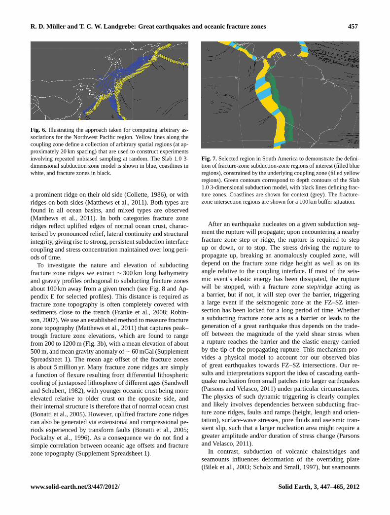
The analysis presented in this paper investigates magnituderelationships between earthquake locations in the vicinityof fracture zone and volcanic chain/ridge intersections withthe coupling zone. The structure of the bathymetric featureswas used to project their extensions into the nearby couplingzone, maintaining the same azimuth as in their oldest geo-physical expressions seaward of a given trench. The resultantintersection is bounded by the width of the coupling zone.This results in linear spatial features that serve as a referencefor undertaking the analysis of associated earthquakes for arange of proximities, allowing the sensitivity of the associ-ation to be quantified. In Fig. 7 fracture-zone intersectionswith subduction zones are shown for a 100 km buffer region,demonstrating how the spatial associations undertaken forthis study are computed. The buffer regions are progressivelyincreased in size to trade-off the strength of the associationwith the specificity of the targeted area, calibrated against theentire coupling zone area.

We apply a type of information filtering system techniquecalled “Top-N analysis”, which is widely used in searching,sorting, classifying, and filtering very large data sets (Cre-monesi et al., 2010) to investigate the association of sig-nificant earthquakes as a function of magnitude with sub-duction coupling zone segments with and without fracturezone or volcanic ridge/chain intersections. This approachsuits the magnitude distribution of earthquakes, where largerevents are more infrequent. The Top-N analysis progres-sively assesses how strongly particular sets of subductionzone segments are associated with sets of sorted earthquakesin a given magnitude range. As the total number of Top-Nearthquakes, from the largest event down to a given cutoffmagnitude, is increased by progressively including smaller-magnitude events, the so-calledrecall is computed, definedas the number of Top-N earthquakes associated with the tar-get coupling zone regions divided byN . The resultant statis-tical measure represents an intuitive description of the effec-tiveness of a given target data set (fracture zone–subductionzone (FZ–SZ) intersections, volcanic ridge/seamount inter-sections, or randomly chosen subduction coupling zone seg-ments) in accounting for the location of significant earth-quakes on record.

The analysis is described formally as follows: the signif-icant earthquakes data set is denoted E, consisting of a listof latitude (θ ), longitude (λ) and magnitude (M) tuples suchthat E= [e1,e2, . . . ,eNe ] for a data set size ofNe, and thei-thelement of E is denotedei = (θei

,λei,Mei

). In this analysis Eis then re-ordered by sorting it in descending order in termsof magnitude, resulting in Es. Target locations are projectedinto the coupling zones as described previously, resulting in



lines traversing the coupling zone. The list ofNt projectedtarget lines pairs is defined as:

Lt = [L1, L2, ..., LN ]. (1)

The Top-N methodology involves computing the ratio ofthe highest-N earthquakes within a specified region of inter-est (ROI), specified by a buffer distancedROI in kilometresaroundLt, denoted the Top-N recall. When studying the re-call for a particularN , the performance evaluation score isdefined as recall-N, and is calculated by summing the num-ber ofN sorted earthquakes (i.e. [e1,e2, . . . ,eN ]) associatedwithin the ROI regions. Formally this procedure involves cre-ating a binary vectorA of lengthN , defined asA = [a1, a2,...,aN ]. The i-th item inA is determined as follows:

ai =

1 ifNt∑

j=1F(es(i),Lj ,dROI,CZ) > 0

0 otherwise

(2)

where CZ is the coupling zone polygon geometry, andF con-siders the association within a thresholded buffer aroundLj

bounded by CZ.

F(es(i),Lj ,dROI,CZ) =

(1 if es(i) inpolygonG(Lj ,CZ,dROI)

0 otherwise

)(3)

The functionG(Lj ,CZ,dROI) creates a buffer polygon ofwidth dROI km aroundLj , clipped by CZ. The target earth-quakees(i) can then be tested for association via a standardpoint-in-polygon test, denotedinpolygon. Now that the bi-nary vectorA has been computed, the recall-N score can bedetermined via

recall=1

N

N∑i=1

ai . (4)

2.5 Sensitivity analysis: ruling out random effects

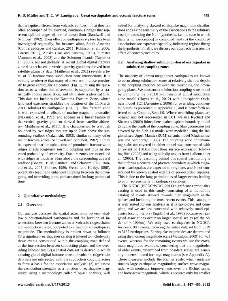
The study objective is to evaluate the nature of significantearthquakes in the vicinity of target locations along subduc-tion zones. It is important to compare the nature of these as-sociations with the “random-association” case (which we callthe arbitrary case) in order to ascertain whether the resul-tant associations could occur at random, and to calibrate thestrength of the association (i.e. the “sensitivity” and “speci-ficity” characteristics). The approach taken is to carry out re-peated analyses along subduction zones in which arbitrarytarget locations are specified. These arbitrary target locationselections are repeated 100 times in a stochastic fashion toascertain respective statistical variability, allowing for a thor-ough ruling out of an association occurring at random (theNull hypothesis pertaining to the topic of this study). Sub-duction coupling zone partitions are generated perpendicularto the coupling zone axis at a spacing of 20 km, providing aset of 2634 partitions (Fig. 6). Each partition element is ex-tended along strike of a given subduction zone using widths

ranging from 50 to 400 km to enable a sensitivity analysiswith regard to spatial proximity of earthquakes and FZ–SZintersections.

The arbitrary case methodology comprises the extractionof a number of points randomly sampled along subduc-tion zones, drawing the same number of random samplesas there are target locations (i.e. 59 fracture-zone intersec-tion locations, and 14 intersections pertaining to major vol-canic chains/ridges, respectively). Thus, a repeated selectionof 59 and 14 virtual target regions is undertaken, followedby the same Top-N association analysis. The process is re-peated 100 times (exceeding this amount resulted in con-sistent statistics), with the statistics from various runs sum-marised via median, and 20th/80th percentile error bars. Thearbitrary case methodology thus repeatedly simulates a simi-lar scenario to the targeted case, providing a relative measureby which the statistical significance of the associations can beascertained for different proximities from the target zones.

2.6 Spatial hazard-zone construction

In order to relate the FZ–SZ intersection regions to a spa-tially meaningful interpretation, it is important to establisha baseline/reference spatial zone that can be compared with.The spatial zone comprises the regions in which all subduc-tion earthquakes are known to occur, i.e. the coupling zonedefined earlier. This allows a direct comparison to be madebetween the regions in which the associations discussed inthis paper are strong, and the entire reference region. Thisapproach also has application to long-term earthquake haz-ard risk assessment. The baseline coupling zone surface areais computed to be∼ 1.088×107 km2, which is about 2.1 % ofthe Earth’s surface area (∼ 51.095×107 km2). The approachevaluates the proportion of earthquakes associated with par-ticular subduction coupling zone sub-regions (e.g. 150 kmwide centred on FZ–SZ intersections). These regions of in-terest form the FZ–SZ target zones, which can then be com-pared to the baseline area to compute its “specificity”, i.e.to what extent the baseline area has been reduced. This isthen assessed together with the association strength (“sensi-tivity”) to obtain a spatially meaningful assessment of the as-sociation strength for different buffer-widths across the cou-pling zones. The computed fraction of the coupling zone areafor chosen buffer widths 50, 100, 150, 200, 250, 300, and400 km, respectively, is presented in Table 1, having beencomputed taking into account the fact that neighbouring re-gions can overlap somewhat.

2.7 Geodetic plate convergence rates

Present-day inter-plate convergence velocities from theGlobal Strain Rate Map Project (Kreemer et al., 2003) areused to estimate the trench perpendicular convergence ratesand azimuths at subduction zones to assess the role of theseparameters in modulating the effect of subduction asperities



Table 1.Calculated areas and fraction of coupling zone for chosenbuffer widths around fracture-zone intersections.

Buffer width Intersection area Percentage of(km) (km2) coupling zone area

50 1.601× 106 14.7100 2.615× 106 24.0150 3.463× 106 31.8200 4.152× 106 38.2250 4.621× 106 42.5300 5.007× 106 46.0400 5.554× 106 51.0

on generating significant earthquakes. Relative convergencespeed and azimuths within 7.5 degrees (in both latitude andlongitude dimensions) of target locations are extracted in or-der to provide sufficient spatial information to accurately de-fine the boundary between the two plates (the grids have a 1degree resolution). The extracted boundary is subsequentlyused to compute smoothed convergence velocities.

3 Results

3.1 Intersections between fracture zones and volcanicridges/chains with subduction zones

The Top-N analysis is initially carried out using a subduc-tion coupling zone segment width of 150 km following theobservation that topographic anomalies associated with frac-ture zones are rarely wider than this (Fig. 8), and accountingfor spatial uncertainties in the projected location of asperi-ties in the coupling zone. The analysis reveals a significantrelationship between FZ–SZ intersections and large earth-quakes (Fig. 2a). For earthquakes with magnitudes largerthan 8.0, the Top-N recall for FZ–SZ intersections divergessharply from the arbitrary case (Fig. 2a), suggesting thatthere is a relationship between great earthquakes and thesubduction of topographic anomalies associated with FZ–SZintersections, and that this correlation becomes more pro-nounced with increasing earthquake magnitudes. For the 50largest earthquakes (Mw ≥ 8.4), 50 % are associated withFZ–SZ intersections as opposed to 25 % of randomly se-lected subduction zone corridors. For the 15 largest events(Mw ≥ 8.6), 13 of which are associated with FZ–SZ inter-sections, the difference rises to about 70 % (Fig. 2b). If frac-ture zones did not play a special role in driving great earth-quakes, we would expect only 3 of the 15 largest subductionearthquakes on record to be associated with coupling zoneregions centred on subducting fracture zones. In contrast, thevolcanic ridge/seamount chain subduction zone intersectionsanalysed here display a far weaker association, and only formagnitudes less than 8, as compared with randomly selectedsubduction zone locations (Fig. 2c, d). We note that this data

set is relatively small (14 intersections), so the associationsdo have substantial uncertainties.

The robustness of our results is tested via a sensitivityanalysis with respect to the width of the coupling zone seg-ments (Fig. 2e, Appendix D). It demonstrates (1) that the15 largest megathrust earthquakes on record (Mw ≥ 8.6) aresignificantly biased towards FZ–SZ intersection regions and(2) that an intersection corridor width of 150 km representsa threshold. As the coupling segment width adjacent to FZ–SZ intersections is widened from 50 to 150 km, there is asteep increase in the association of the top 15 earthquakeswith FZ–SZ intersection coupling zones, whereas a furtherincrease in coupling zone width does not capture any ad-ditional events (Fig. 2e). A similar association is still visi-ble for the top 50 (Mw ≥ 8.4) earthquakes, with an inflec-tion point at a corridor width of 150 km (Fig. 2e), leading tothe conclusion that great earthquakes with magnitudes largerthan 8.4 are preferentially associated with subduction cou-pling zone regions 150 km wide centred on FZ–SZ intersec-tions. The initial Top-N analysis (Fig. 2a, b) suggests that thisrelationship holds for all great earthquakes (Mw ≥ 8.0), butfor events with magnitudes between 8.0 and 8.4 the associa-tion is not as clearly dependent on the fracture zone corridorwidth. Previous studies have suggested that subduction earth-quake size distributions may depend on convergence rates(McCaffrey, 1994; Gutscher and Westbrook, 2009; Ruff andKanamori, 1983). Our analysis reveals that all subductionearthquakes with magnitudes of 7 and more at FZ–SZ in-tersections are associated with relatively high mean conver-gence rates of about 65 mm a−1, whereas great earthquakesat FZ–SZ intersections with magnitudes over 8.5 are distin-guished by their link with relatively shallow mean slab dipangles (measured directly below a given earthquake epicen-tre) of around 20◦, but smaller significant earthquakes occurover wide ranges of slab dips, with relatively shallow meandips of 23–27◦ (Fig. 3a). These observations lead to the con-clusion that very shallow slab dips (∼ 20◦) combined withsubducting fracture zones give rise to particularly large greatearthquakes.

3.2 Long-term great subduction earthquake hazardmap

Applying the Top-N association analysis in the context of thespatial hazard map shows that 87 % of the 15 largest, halfof the largest 50 and 44 % of the largest 100 earthquakesare associated with FZ–SZ intersections, an area restrictedroughly to 32 % of the subduction coupling zone (Fig. 5 andTable 1). There is a long-standing controversy over whetherthe present state of seismological science inhibits reliabledifferentiation of the risk level in particular geographic ar-eas along subduction zones, or whether the feasibility ofassessing at least the long-term regional earthquake poten-tial is promising in principle, based on long-term earthquakeactivity and the plate tectonic setting (Sykes et al., 1999).



a

��

��

��

�

�

�

�

�

� ��

��

��

��

��

��

��

��

��

��

�� ! �� "!#�"��$

% � ≥��

��&�%$ ≤��

��&�%$≤�� % �&��$

$

��

��

��

�

�

��

��

� ��

��

��

��

��

��

��

��

��

��

�� ! �� "!#�"��$

��

��

��

�

�

%$� ≥��

��&�%$� ≤��

��&�%$�

≤�� %$�&��

� ��

��

��

��

��

��'!�� "��(�� ! �� "!#�"��$

��

��

��

�

�

� ��

��

��

��

��

��

'!�� "��(�� ! �� "!#�"��$

��

��

0.1 0.2 0.3 0.4 0.5 0.60

0.1

0.2

0.3

0.4

0.5

0.6

0.7

0.8

0.9

1

Fraction of coupling zone area

Rec

all

TopN−10TopN−15TopN−20TopN−25TopN−50TopN−75TopN−100TopN−250

50km

100km

150km 200km 250km 300km 400km

a b

c d

e

Fig. 2. (a)Evaluation of coupling-zone filtered earthquake associations with intersections between 59 fracture zones and subduction zones,sorted by magnitudeN and using a buffer of 150 km on either side of the projected fracture zone. The sorted event magnitudes are plottedagainst therecall, the number of Top-N earthquakes associated with the fracture zone intersection regions divided byN ; this is comparedwith the same number (59) of randomly generated subduction zone intersection segments drawn from the global coupling one, repeated 100times for the entire filtered earthquake data set, shown as median values with the 20th/80th percentile error-bars;(b) same as(a) but for thetop 100 (Mw ≥ 8.1) significant earthquakes;(c, d)same as(a, b) for volcanic ridge/chain intersections with subduction zones;(e) top-N greatearthquake analysis in proximity of subduction zones illustrating the baseline-normalized recall (sensitivity) traded off against the reductionin hazard surface area (% of original hazard area, all subduction earthquakes), called the hazardspecificity. Note the sharp inflection pointfor the top 15 earthquakes at 150 km, illustrating that 87 %, i.e. 13 out of 15 largest earthquakes, all occurred within 150 km of a FZ–SZintersection.

McCaffrey (2007, 2008) goes as far as to suggest that givena long enough subduction trench and sufficient time, giantearthquakes may well happen at any subduction zone. Ouranalysis provides overwhelming evidence that FZ–SZ inter-sections are associated with a significantly elevated proba-bility of long-term great earthquakes as compared to the re-mainder of subduction segments, confirming that knowledge

of the tectonic setting can help differentiate long-term re-gional earthquake risk (Sykes et al., 1999). Our results there-fore provide a way to objectively test long-term earthquakehazard maps, a need discussed extensively after the 2011Tohoku-Oki event that was not predicted by previous hazardmaps (Stein et al., 2011, 2012; Avouac, 2011; Geller, 2011).



(a)��

�

��

��

��

��

��

��

��≤��

��≤��

�≤��

��

� !

" ��#��"#$��"��

�

�

��

��

��

��

��

��

%&�'"

(��)*��#��

��+*��

�

,�+"#�#��

,�+"#�#�

-�"�

��

.�/)#��

.�/)#��

��)�

0�1�� 2��

3� 4#++�

��

�#��

5"�

6

Chile Mw 9.5

Chile Mw 9.5

SumatraMw 9.1 Japan

Mw 9.0

Chile Mw 8.8

Peru Mw 8.8/8.6

Rat Islands Mw 8.7

Peru Mw 8.7/8.6

Chile Mw 8.7

Adak Islands Mw 8.6

a

b

(b)

��

�

��

��

��

��

��

��

��≤��

��≤��

�≤��

��

� !

" ��#��"#$��"��

�

�

��

��

��

��

��

��

%&�'"

(��)*��#��

��+*��

�

,�+"#�#��

,�+"#�#�

-�"�

��

.�/)#��

.�/)#��

��)�

0�1�� 2��

3� 4#++�

��

�#��

5"�

6

Chile Mw 9.5

Chile Mw 9.5

SumatraMw 9.1 Japan

Mw 9.0

Chile Mw 8.8

Peru Mw 8.8/8.6

Rat Islands Mw 8.7

Peru Mw 8.7/8.6

Chile Mw 8.7

Adak Islands Mw 8.6

a

b

Fig. 3. (a)Filtered earthquakes grouped in five magnitude categories plotted as a function of median slope of the subduction coupling zone(Hayes et al., 2012) versus the median (trench perpendicular) geodetic convergence rates (Kreemer et al., 2003), with error-bars depicting20th/80th percentiles.(b) Elevation of fracture zone ridges relative to the adjacent ocean floor for the 13 largest earthquakes on recordassociated with FZ–SZ intersections amongst the top 15 events (see Figs. 1 and 2). Bathymetry profiles∼ 300 km in length were extracted∼ 100 km seaward of the trench, perpendicular to fracture zones. Fracture zone ridge heights were computed by measuring the total heightbetween ridge crests and fracture zone valleys.

A local subducting fracture zone alone may not be suf-ficiently noteworthy to suspect a link with seismic hazardswithout having recognised a strong global link between sub-ducting fracture zones and great earthquakes, as demon-strated here. This connection provides critical additional in-formation for seismologists to pinpoint particular tectonicenvironments that are more prone to strong seismic couplingand great earthquake supercycles than average subductionsettings. Candidate locations (Fig. 5) for such earthquake su-percycles will need to be scrutinized in greater detail, includ-ing their historical earthquake records and geological datasuch as co-seismically displaced coral reefs (Taylor, 2011;Sieh et al., 2008) and prehistoric tsunami deposits (Satake etal., 2003). We identify a total of 25 candidate regions, locatedalong the Java, Japan, Aleutian, Central and South American,Scotia, Lesser Antilles and Cascadia trenches (Fig. 5).

Our results suggest the possibility that the Tohoku-Oki2011 giant earthquake cycle, and the related distributed setof asperities (Tajima and Kennett, 2012), may be related tostrong coupling due to the obliquely subducting KashimaFracture Zone (Fig. 1), whose offshore location is wellmapped, mainly based on ship marine magnetic and seis-mic reflection data (Nakanishi, 1993; Nakanishi et al., 1992).Its association with subduction earthquake cycles has notbeen investigated. It is, however, conceivable that a veryobliquely subducting, fracture zone ridge with varying ele-vation along the strike, as is common for large fracture zoneridges (Tucholke and Schouten, 1988; Cande et al., 1995;Croon et al., 2008), causes subduction zone segmentation asobserved by Tajima and Kennett (2012). We regard this asmore likely than a subducting seamount to be responsible for

the Tohoku-Oki 2011 event, as suggested by Duan (2012),given that there is no observational evidence for a subduct-ing seamount close to its epicentre, including no sign of anyseamount chain intersecing the subduction zone in the vicin-ity of the epicentre. The closest seamount chain is subductingabout 200 km to the south of the Tohoku-Oki 2011 epicentre(Duan, 2012). The 300 km long asperity recently mapped byHashimoto et al. (2012) may possibly reflect the subductingKashima fracture zone.

The Cascadia margin is of particular interest in this con-text, because there is circumstantial evidence that the mainarea of slip of the great 1700 Cascadia earthquake was cen-tred on the intersection of the southern Cascadia margin withthe Blanco Fracture Zone (Fig. 1). Satake et al. (2003) com-pare 6 Cascadia rupture models, which they rank based onpaleoseismological evidence and comparisons between mod-elled tsunami heights in Japan. Amongst alternative displace-ment models for the northern, central and southern Cascadiasubduction zone, the southern model, which extends 440 kmsouthward from central Oregon to northern California withan average slip of 21 m, is the most effective in terms of ac-counting for tsunami run-up in Japan (Satake et al., 2003).Even though this model does not account for the entire pat-tern of coastal subsidence following this event (Leonard etal., 2010), these results raise the possibility that subductionof a fracture zone ridge may have played a role in trigger-ing the 1700 event. The Blanco Ridge, associated with thelarge-offset (350 km) Blanco Fracture Zone, displays reliefof up to 1 km (Embley and Wilson, 1992). Its extension to theCascadia margin has been interpreted as continuing in a rela-tively straight fashion to the southern Oregon margin, where



the Blanco slide has been mapped (Goldfinger et al., 2000),and this is confirmed by satellite gravity data (Sandwell andSchubert, 1982). The massive failure of the southern Oregonslope, where the Blanco fracture zone intersects the subduc-tion zone, is expressed by consecutive slide events, and hasbeen interpreted as the result of subduction of a linear ridge,as opposed to subduction of a nearby seamount province, asseamount subduction elsewhere suggests that the typical up-per plate expression of a subducted seamount is a relativelynarrow deformation trail, unlike the large slope failures ofsouthern Oregon (Goldfinger et al., 2000). This linear ridgewould in all likelihood correspond to the Blanco Ridge, inwhich case the 1700 Cascadia megathrust event would fit ourglobal observations and conceptual model.

There are no FZ–SZ intersections along the Philippines,Marianas, Tonga-Kermadec or any of the Southwest Pacifictrenches (Fig. 5). This does not rule out great subductionearthquakes along any of the latter subduction zones, butevents in these regions would not be due to an associationwith a fracture zone intersection. Our analysis shows thatdata mining techniques primarily developed for extractinguseful knowledge hidden in enormous volumes of electronicdata on the Internet have great potential for the analysis oflarge, multidimensional and statistically skewed sets of geo-logical and geophysical data. Recognising the connection be-tween the subduction of fracture zones and great earthquakesglobally has the potential to transform long-term earthquakehazard map generation.

4 Great earthquake rupture propagation and fracturezone ridges

We review rupture propagation associated with FZ–SZ inter-sections during three well-mapped great earthquake eventsto evaluate the role of subducting fracture zone ridges in thetime-dependence of stress release during great earthquakes.During the 2004 Sumatra-Andaman earthquake (Mw 9.1)the rupture was initiated on the seismically imaged subduct-ing Simeulue Ridge, which is 60 km wide, elevated by 1 kmon its western flank, and up to 3 km along its eastern flank(Franke et al., 2008). The ridge is a buried extension of theso-called 96◦ Fracture Zone (Kopp et al., 2008) (Fig. 4a)and defines a major segment boundary for the great 2004Sumatra-Andaman earthquake associated with a step in theslab east of the ridge (Franke et al., 2008). The 2004 eventwas initiated on the western flank of the subducting SimeulueRidge (Fig. 4a), and simultaneously climbed eastwards ontothe crest of the ridge, while also propagating to the northwestand southwest onto a double fracture zone system called the94◦ and 93◦ fracture zones (Kopp et al., 2008), then crossingthese and initiating a separate rupture along an unnamed frac-ture zone west of the 93◦ fracture zones (Fig. 4a). The major-ity of slip distribution during the event is associated with thefour fracture zones involved in the rupture, suggesting that

Fig. 4. Three great earthquake rupture case studies for(a) the 2004Mw = 9.1Sumatra-Andaman Earthquake (Robinson, 2007) and(b) the 2001Mw = 8.4 Peru earth-quake (Robinson, 2007) depicting the modelled rupture process through time for 5 mslip contours, and(c) the 1986Mw = 8.0 Andreanoff islands earthquake (Das andKostrov, 1990) showing the modelled rupture process through time for a moment-magnitude contour of3×1020 Nm. Earthquake epicentres are shown as red stars, over-lain over vertical gravity gradient maps (Sandwell and Smith, 2009), with fracture zonelocations (Matthews et al., 2011) shown as yellow dashed lines, with their interpretedcoupling zone extensions outlined in faint yellow dashes. Coloured polygons illustratethe progression of the rupture process relative to the inception at the epicentre, pro-viding a visualisation of the role that the fracture zones played during the event. Insetplots show ship bathymetry (top) and gravity anomalies (bottom) along magenta pro-files crossing key fracture zones, with red arrows indicating fracture zone location. Theseismically imaged Simeulue ridge (Franke et al., 2008), associated with the subducting96◦ Fracture Zone (Kopp et al., 2008), is outlined as black dashed line.



90˚E

90˚E

120˚E

120˚E

150˚E

150˚E

180˚

180˚

150˚W

150˚W

120˚W

120˚W

90˚W

90˚W

60˚W

60˚W

60˚S 60˚S

30˚S 30˚S

0˚ 0˚

30˚N 30˚N

60˚N 60˚N

Kam S

Z

Jap

SZM

ar. S

Z

Phi

l SZ

Aleu SZ

To-K

e S

Z

Cas SZ

S-A

m S

Z

C-Am SZ

SW-P SZJava SZ

Jap S

Z L-An SZ

Fig. 5. ETOPO1 global relief map (Robinson projection) withoceanic fracture zones shown as black lines. Global subductioncoupling zone (solid blue regions) is overlain with fracture zone-subduction zone intersection regions (solid red bands), significantlymore prone to great earthquakes than the blue bands, based on ouranalysis. Intersections between volcanic chains/ridges (solid yellowbands) are biased towards an above-average occurrence of smallerearthquakes, but this result is more uncertain due to the relativelysmall number of these intersections. Overlain are the largest 15 in-strumentally recorded earthquakes (Mw = 8.6) (white filled stars)and the largest 50 earthquakes (Mw = 8.4) (while filled circles).Subduction zone labels as in Fig. 1.

the associated fracture zone ridges represent anomalouslycoupled regions due to their elevation associated with a shal-low slab dip (Supplement Spreadsheet 1).

The 2001 Peru earthquake (Mw 8.4) nucleated near the topof the Nazca fracture zone lateral ramp, briefly stalling on theNazca ramp before stepping down the ramp, breaking the ad-jacent flat segment and finally stopping at the Iquique ridgeramp (Carena, 2011; Robinson et al., 2006) (Fig. 4b). Thefracture zone increased plate coupling between the two sidesof the fault, resulting in a heterogeneous rupture, with themain stress release focussed on the Nazca FZ–SZ intersec-tion (2006) (Fig. 4b). There are alternative slip models forthis event, but we did not find published models that showeither slip or energy release as a function of time after theevent.

The 1986 Andreanof Islands (Aleutians) earthquake (Mw8.0) rupture history is available as computed moment releasethrough time (Das and Kostrov, 1990). It illustrates that thisevent was initiated on a subduction segment bounded by theAdak and Amlia fracture zones (Lu and Wyss, 1996), beforepropagating west and climbing onto a ridge adjacent to theAdak fracture zone (Fig. 4c) where the main moment releasewas concentrated. This event represents an example wheremost of the elastic energy was dissipated by the rupture prop-agating onto the strongly coupled Adak fracture zone ridge,with a peak–trough topographic elevation of over 1000 m

(Fig. 8), preventing the rupture from propagating far into thenext segment.

5 Physical model for fracture zone–subduction zoneinteraction

Global analyses for how fracture zones and other aseis-mic ridges may relate to the occurrence of large earth-quakes were first carried out by Mogi (1969), who sug-gested that great shallow earthquakes preferentially occur onlocal depressions. In another global analysis, Kelleher andMcCann (1976) concluded that where bathymetric rises orirregularities interact with active trenches the largest shal-low earthquakes are generally smaller and less frequentthan events along adjoining segments of the plate boundary.These conclusions are contradictory to our results; however,it needs to be kept in mind that global analyses of all subduc-tion zone asperities will likely not reflect a single physicalmechanism.

Studies focussed on the role of fracture zones in seismichazard generation have largely focussed on their regional rolein segmenting subduction zones by providing barriers, sepa-rating adjacent subduction segments from each other, thuscontaining ruptures to individual segments (Bilek, 2010). Luand Wyss (1996) analysed the segmentation of the Aleu-tian plate boundary and found that the regional segmenta-tion boundaries are controlled by subducting fracture zone,which they interpreted as zones of weakness across whichstress may not be transmitted fully. Based on an equivalentstudy of four segments and their barriers along the CentralChile subduction zone, Metois et al. (2012) concluded thatthe segments are characterised by higher coupling and sepa-rated by narrow areas of lower coupling. If this model heldtrue globally, then we would observe precisely the oppositeof what we find, namely great earthquakes should be biasedtowards subduction segments between fracture zones and thesegments centred on fracture zones should be biased againstlarge seismic events.

These three great earthquake rupture histories, togetherwith our global analysis, lead to the following model forwhy subducting fracture zones are frequently associatedwith great seismic events. Fracture zones in cross-sectionform either large steps or represent valleys bounded by to-pographic ridges; these two morphologies are known as“Pacific-type” and “Atlantic-type” fracture zones (Matthewset al., 2011). Pacific-type large-offset fracture zones displayelevation steps in cross-section due to age-offsets at trans-form faults, where a given fracture zone originates, and thesesteps are enhanced by flexure due to differential coolingand thermal lithospheric contraction and associated flexu-ral bending, producing flexural ridges (Sandwell and Schu-bert, 1982) whose internal structure is identical to that ofnormal ocean crust. In contrast, Atlantic-type small-offsetfracture zones are characterised by asymmetric valleys with



Fig. 6. Illustrating the approach taken for computing arbitrary as-sociations for the Northwest Pacific region. Yellow lines along thecoupling zone define a collection of arbitrary spatial regions (at ap-proximately 20 km spacing) that are used to construct experimentsinvolving repeated unbiased sampling at random. The Slab 1.0 3-dimensional subduction zone model is shown in blue, coastlines inwhite, and fracture zones in black.

a prominent ridge on their old side (Collette, 1986), or withridges on both sides (Matthews et al., 2011). Both types arefound in all ocean basins, and mixed types are observed(Matthews et al., 2011). In both categories fracture zoneridges reflect uplifted edges of normal ocean crust, charac-terised by pronounced relief, lateral continuity and structuralintegrity, giving rise to strong, persistent subduction interfacecoupling and stress concentration maintained over long peri-ods of time.

To investigate the nature and elevation of subductingfracture zone ridges we extract∼ 300 km long bathymetryand gravity profiles orthogonal to subducting fracture zonesabout 100 km away from a given trench (see Fig. 8 and Ap-pendix E for selected profiles). This distance is required asfracture zone topography is often completely covered withsediments close to the trench (Franke et al., 2008; Robin-son, 2007). We use an established method to measure fracturezone topography (Matthews et al., 2011) that captures peak–trough fracture zone elevations, which are found to rangefrom 200 to 1200 m (Fig. 3b), with a mean elevation of about500 m, and mean gravity anomaly of∼ 60 mGal (SupplementSpreadsheet 1). The mean age offset of the fracture zonesis about 5 million yr. Many fracture zone ridges are simplya function of flexure resulting from differential lithosphericcooling of juxtaposed lithosphere of different ages (Sandwelland Schubert, 1982), with younger oceanic crust being moreelevated relative to older crust on the opposite side, andtheir internal structure is therefore that of normal ocean crust(Bonatti et al., 2005). However, uplifted fracture zone ridgescan also be generated via extensional and compressional pe-riods experienced by transform faults (Bonatti et al., 2005;Pockalny et al., 1996). As a consequence we do not find asimple correlation between oceanic age offsets and fracturezone topography (Supplement Spreadsheet 1).

Fig. 7. Selected region in South America to demonstrate the defini-tion of fracture-zone subduction-zone regions of interest (filled blueregions), constrained by the underlying coupling zone (filled yellowregions). Green contours correspond to depth contours of the Slab1.0 3-dimensional subduction model, with black lines defining frac-ture zones. Coastlines are shown for context (grey). The fracture-zone intersection regions are shown for a 100 km buffer situation.

After an earthquake nucleates on a given subduction seg-ment the rupture will propagate; upon encountering a nearbyfracture zone step or ridge, the rupture is required to stepup or down, or to stop. The stress driving the rupture topropagate up, breaking an anomalously coupled zone, willdepend on the fracture zone ridge height as well as on itsangle relative to the coupling interface. If most of the seis-mic event’s elastic energy has been dissipated, the rupturewill be stopped, with a fracture zone step/ridge acting asa barrier, but if not, it will step over the barrier, triggeringa large event if the seismogenic zone at the FZ–SZ inter-section has been locked for a long period of time. Whethera subducting fracture zone acts as a barrier or leads to thegeneration of a great earthquake thus depends on the trade-off between the magnitude of the yield shear stress whena rupture reaches the barrier and the elastic energy carriedby the tip of the propagating rupture. This mechanism pro-vides a physical model to account for our observed biasof great earthquakes towards FZ–SZ intersections. Our re-sults and interpretations support the idea of cascading earth-quake nucleation from small patches into larger earthquakes(Parsons and Velasco, 2011) under particular circumstances.The physics of such dynamic triggering is clearly complexand likely involves dependencies between subducting frac-ture zone ridges, faults and ramps (height, length and orien-tation), surface-wave stresses, pore fluids and aseismic tran-sient slip, such that a larger nucleation area might require agreater amplitude and/or duration of stress change (Parsonsand Velasco, 2011).

In contrast, subduction of volcanic chains/ridges andseamounts influences deformation of the overriding plate(Bilek et al., 2003; Scholz and Small, 1997), but seamounts



0 50 100 150 200 250 300 350−5000

−4900

−4800

−4700

−4600

−4500

−4400

Profile distance (km)

Bat

hym

etry

(m

)

0 50 100 150 200 250 300 350−6100

−6000

−5900

−5800

−5700

−5600

−5500


Bat

hym

etry

(m

)

0 50 100 150 200 250 300 350−6000

−5950

−5900

−5850

−5800

−5750

−5700

−5650

−5600

−5550


Bat

hym

etry

(m

)

0 50 100 150 200 250 300 350−4500

−4400

−4300

−4200

−4100

−4000

−3900

−3800

−3700


Bat

hym

etry

(m

)

0 50 100 150 200 250 300 350 400−5000

−4800

−4600

−4400

−4200

−4000

−3800


Bat

hym

etry

(m

)

0 50 100 150 200 250 300 350−5800

−5600

−5400

−5200

−5000

−4800

−4600

−4400


Bat

hym

etry

(m

)

0 50 100 150 200 250 300 350−4800

−4700

−4600

−4500

−4400

−4300

−4200

−4100


Bat

hym

etry

(m

)

0 50 100 150 200 250 300 350−4600

−4500

−4400

−4300

−4200

−4100

−4000

−3900

−3800

−3700

−3600


Bat

hym

etry

(m

)

0 50 100 150 200 250 300 350−4200

−4100

−4000

−3900

−3800

−3700

−3600

−3500

−3400


Bat

hym

etry

(m

)

0 50 100 150 200 250 300 350−4600

−4400

−4200

−4000

−3800

−3600

−3400

−3200

Profile distance (km)B

athy

met

ry (

m)

0 50 100 150 200 250 300 350 400−5700

−5600

−5500

−5400

−5300

−5200

−5100

−5000


Bat

hym

etry

(m

)

Valdivia2 Valdivia

Salang

Kashima2

Kashima Mocha

Naza

Rat

Trujillo Santiago

Adak

Fig. 8. Bathymetric profiles across the 11-identified fracture zonesassociated with the 13 largest of the top 15 earthquakes in the cou-pling zone.

are known to result in weak seismic coupling (Mochizukiet al., 2008; Singh et al., 2011), and this is confirmed byour observations (though we acknowledge we are limited inconfidence due to a limited number of identified volcanicchain/ridge intersections). Seismic studies of seamounts haverevealed their complex internal layering structure, and theirseparation from the underlying ocean crust by a decollementsurface, both contributing to their disintegration and shear-ing off during subduction (Das and Watts, 2009), and thuspreventing them from initiating strong local coupling at thesubduction interface. As a consequence the seismogenic be-haviour of subducting seamounts is controlled by the devel-opment of an adjacent fracture network during subduction(Wang and Bilek, 2011). The complex structure and hetero-geneous stresses of this network provide a favourable con-dition for aseismic creep and small earthquakes, but an un-favourable condition for the generation and propagation oflarge ruptures (Wang and Bilek, 2011). Our results supportthis model overwhelmingly, as subducting volcanic ridgesand chains are found to be associated with an excess of rel-atively small seismic events (magnitude< 8), but not greatearthquakes, suggesting that subducting volcanic edifices arenot able store significant stress, as stress is released either insmall earthquakes, or aseismically.

6 Conclusions

We have investigated well-defined fracture-zones and vol-canic chains/ridges and seamounts that are in the processof being subducted, and their associations with the locationsof significant earthquakes. Linking subducting bathymetricfeatures with large earthquakes is a particularly interestingquestion, since if recurrence-cycles are indeed several hun-dreds of years in duration, then hazard predictions meth-ods involving the use of existing data may be ineffective atpredicting many of the more devastating events. The anal-ysis involved investigating the associations as a function ofeathquake magnitude, making use of a data-mining method-ology called “Top-N” analysis for coping with the statisti-cally skewed nature of earthquake magnitude distributions.The analysis investigated the associations in the couplingzones between subducting and overriding plates using recent3-dimensional data sets, and utilised a comprehensive sen-sitivity analysis of computation of the arbitrary case to thor-oughly test the null hypothesis, i.e. that the associations couldoccur at random. The results in this paper revealed a strikingassociation between fracture-zone/subduction-zone intersec-tions, and the very largest subduction-events on record, withthe effect diminishing as magnitudes decrease below mo-ment magnitude 8.0. A similar effect was not demonstratedby volcanic chains/ridges and seamounts, but the conclusionsare limited by a small data set size. The analysis went onto demonstrate that the most important fracture zones gen-erally have very large physical offsets, which could play



Fig. B1. Regional tectonic settings and key data for the East In-dian Ocean region. The following colour schemes are used, dif-fering slightly to those in Fig. 1 of the main paper for enhancedbackground contrast: subduction zones (blue bands), intersectionpoints of fracture zones with subduction zones (yellow squares),intersection points of the volcanic chains and ridges with subduc-tion zones (green squares), largest 25 earthquakes (red stars), earth-quakes magnitude 8.3 and above (light blue circles), all other sig-nificant earthquakes (small brown circles). The Sandwell and Smithvertical-gravity gradient grid (Sandwell and Smith, 2009) is shownin the background. Conic equidistant projections are used through-out.

an important role in influencing the subduction coupling.Three modelled rupture events were then discussed, with thespatiotemporal nature of the rupture propogations correlatedwith the approximate physical locations of the fracture zones.This analysis could have important implications for the field.

Appendix A

Earthquake catalogue pre-processing

The NGDC global Significant Earthquakes database(NGDC/WDC, 2011) is used to investigate its relationshipwith particular subduction zone target areas. This databaseconsists of 5539 recorded earthquakes considered to besignificant in magnitude. Several magnitude measurementscales are used in this data set, with modern earthquakesbased on the Moment Magnitude scale (McCalpin, 2009),whereas magnitudes of older records make use of scales suchas the Richter scale (which underestimates large earthquakemagnitudes). Other scales are also used as follows:

– Surface wave magnitude, which improves on theRichter scale to some extent.

– Body-wave magnitude – this scale is less accurate forsmaller magnitude events.

Fig. B2. Tectonic setting and key data for the Japan region. SeeFig. B1 for legend.

Fig. B3. Tectonic setting and key data for the Central Americanregion. See Fig. B1 for legend.

Appendix B

Regional maps

In this study it is important to retain as large a data set as pos-sible for maximum confidence. The approach chosen is to usethe Moment Magnitude measurements by default, of whichonly 761 of the 5539 observations are valid. The remainderof observations use any of the remaining magnitude mea-surements, utilising the maximum of these values. This is inline with the under-estimating nature of the older, more obso-lete scales for large earthquakes. We argue that this approachis valid because small differences in magnitudes would notsignificantly affect the outcomes of this study. An exceptionis observations associated with an intensity measure, typi-cally estimated for historic earthquakes via indirect methods.These observations are removed. Using this approach, thepre-processed NGDC data set reduces to 3684 samples. Thisdata set is subsequently filtered using the methodology de-scribed in Sect. 3 to retain only those earthquakes originatingin the subduction coupling zone, further reducing the data setto 1073 samples.



Fig. B4. Tectonic setting and key data for the Aleutian and Kam-chatka regions. See Fig. B1 for legend.

Fig. B5. Tectonic setting and key data for the Alaskan region. SeeFig. B1 for legend.

Figures B1, B2, B3, B4, B5 and B6 present a number ofregional maps detailing the tectonic settings where fracture-zone/subduction-zone (FZ–SZ) interactions are prominent.These include: the East Indian ocean region along the Java-Sunda trench; the Japanese region; the Aleutian and Alaskanregions considering the geological settings proximal to theKamchatka and Aleutian subduction-zones, together with anumber of prototypical fracture-zone intersection locationsassociated with large earthquakes; the Central American andSouth American regions depict numerous target locationsalong the Andes and Central America. The various plots aresuperimposed on the Sandwell and Smith vertical-gravitygradient grid (Sandwell and Smith, 2009), as was used inlocating and digitising fracture-zones.

Fig. B6. Tectonic setting and key data for the Central Americanregion. See Fig. B1 for legend.

Appendix C

Constructing a global lithosphere-subductioncoupling zone

The interface between the overriding lithosphere and thedown-going slab is the coupling zone in which shallowmega-thrust earthquakes occur. In this study the couplingzone is isolated in 3-dimensions, allowing earthquake cat-alogs to be filtered out. This enables us to compute slabdip in the coupling zone, allowing associations to be as-sessed comparing flat-slab to steep-slab subduction settings.In this global study we have made use of the NOAA sig-nificant earthquakes catalog to investigate relationships be-tween subducting fracture zone and volcanic ridges/chainswith subduction thrust-type earthquakes. It is important toisolate only those earthquakes occurring in the couplingzone at the interface between the overriding and downgo-ing plates. The approach taken is to use recent global mod-els and data sets to localise these 3-dimensional structures,capitalising on the recent publication of the Slab 1.0 3-dimensional subduction model (Hayes et al., 2012), as wellas a number of other data sets, described below. Surface-expressions of subduction zones form the upper boundaryof the coupling zone, defined from the global plate bound-ary dataset (Bird, 2003). Corresponding three-dimensionalmodels are extracted via the Slab 1.0 3-dimensional globalsubduction zone model (Hayes et al., 2012). Since the Slab1.0 model did not cover all regions defined by the globalplate boundary data set, missing regions were modelled us-ing the Regionalised Upper Mantle (RUM) seismic model(Gudmundsson and Sambridge, 1998). A few remainingregions were assumed to extend 150 km from their surface



Fig. C1. Illustration of the intersection between a lithosphere thick-ness model of the overriding plate with a 3-dimensional slab model(coloured contours). Green colours reflect the subduction couplingzone, here conservatively taken as the entire intersection region be-tween the overriding and downgoing plates, and red colours reflectthe slab surface below the lithosphere-asthenosphere boundary ofthe overriding plate. The black points define the edge of the cou-pling zone.

expressions, according to global average estimates of slabgeometry pertaining to the upper regions of subducting slabs(up to 125 km in depth with 30–50◦ subduction dips), as dis-cussed in Lallemand et al. (2005). Intersecting models of theLithosphere–Asthenosphere Boundary (LAB) with recent 3-dimensional representations of subduction zones allows cou-pling zone regions to be defined. The LAB is defined us-ing a combination of continental and oceanic models. Thecontinental model makes use of the global thermal modelTC1 (Artemieva, 2006), in which the 1300 degree isothermis a standard proxy for the LAB. The oceanic model makesuse of the approach in Rychert and Shearer (2009) to es-timate thicknesses in regions not represented by the TC1data set. A nearest-neighbour interpolation is used to makeuse of the nearest available measurements. Thus construct-ing the overall coupling zone involved the integration of 5global data sets. The coupling zone model is referred to as the“CouplingZone1.0” data set. The intersection of the Slab 1.0model with the LAB model is derived by calculating the 3-dimensional intersection between the two models. In Fig. C1the approach taken to intersect the continental model with the3-dimensional slab model is illustrated in an example region.

Appendix D

Fracture-zone intersection Top-N sensitivityanalyses results

The complete results for the Top-N fracture-zone intersec-tion experiments are shown in Fig. D1. These depict both the

N−largest earthquakes

Rec

all

0 200 400 600 800 10000

0.1

0.2

0.3

0.4

0.5

0.6

0.7

0.8

0.9

1FZ intersectionsRandom draws


Rec

all

0 200 400 600 800 10000

0.1

0.2

0.3

0.4

0.5

0.6

0.7

0.8

0.9



Rec

all

0 200 400 600 800 10000

0.1

0.2

0.3

0.4

0.5

0.6

0.7

0.8

0.9



Rec

all

0 200 400 600 800 10000

0.1

0.2

0.3

0.4

0.5

0.6

0.7

0.8

0.9



Rec

all

0 200 400 600 800 10000

0.1

0.2

0.3

0.4

0.5

0.6

0.7

0.8

0.9



Rec

all

0 200 400 600 800 10000

0.1

0.2

0.3

0.4

0.5

0.6

0.7

0.8

0.9



Rec

all

0 200 400 600 800 10000

0.1

0.2

0.3

0.4

0.5

0.6

0.7

0.8

0.9


50km width 100km width



400km width

Fig. D1. Top-N sensitivity analysis, demonstrating substantial andsignificant differences between fracture-zone/subduction-zone in-tersections and the arbitrary case, insensitive to the associationproximity thresholds.

fracture-zone intersection Top-N analyses and arbitrary casesfor the full set of buffer widths used.

Appendix E

Supplementary results for fracture-zone profiles

Bathymetric and gravitational profiles were extracted per-pendicular to digitised fracture zones in the vicinity of thetrench. The profiles extracted were roughly 300 km in length,with the centres coinciding with the digitised fracture zonelocations. Bathymetric and gravitational profiles were anal-ysed simultaneously to localise the trench in the recoveredsignals. Anomaly heights were computed by measuring thetotal height between the lower and upper crests manually.Automatic procedures were ruled out due to the existence ofmultiple significant bathymetric features near-trench.



0

10

20

30

40

50

60

70

80

90

FZ

Id

Gravity anomaly (mGal)

Valdivia2

Valdivia

96degree

Kashima2

Kashima

Mocha

Nazca

Rat

Trujillo

Santiago

Adak

Fig. E1. Gravity anomalies associated with the fracture zones cor-responding to those shown in Fig. 3b.

As listed in Supplement Spreadsheet 1, 11 fracture zoneswere found to be associated with 13 of the largest 15 earth-quakes in the filtered catalogue. In Fig. 8 bathymetric profilesare shown attributed to these 11 fracture zones. In Fig. E1 therespective gravity anomaly values for the 11 highlighted frac-ture zones are shown, complementing the results in Fig. 3bof the main text. A good correlation between the two resultscan be observed, which is expected.

Appendix F

Digital data set descriptions

A number of digital data sets are provided in ESRI shapefileformat, described as follows:

– CouplingZone1p0: the computed CouplingZone1.0 dataset.

– FZ intersections: polyline dataset with fracture zone in-tersections projected across the coupling zone followingthe direction of the digitised fracture zones.

– FZ intersections Buffer 150 km: polygon data set con-sisting of a 150 km buffer around the FZ intersectionsdata set, clipped by the coupling zone.

– SeamountChain intersections: polyline data set withseamount chain/volcanic ridge intersections projected

across the coupling zone following the direction of thedigitised features.

– SeamountChain intersections Buffer 150 km: polygondata set consisting of a 150km buffer around theSeamountChain intersections data set, clipped by thecoupling zone.

Appendix G

Primary statistics

The attached file “Spreadsheet1.xlsx” is a Microsoft Excelspreadsheet containing important statistics computed in thisstudy. Two spreadsheet tabs summarise fracture zone andseamount chain/ridge data, respectively, listing the latitude-longitude locations obtained. The following statistics are tab-ulated for the fracture-zone intersections:

– Name: Fracture zone name.

– Maximum associated magnitude within 250 km: themoment magnitude of the largest earthquake within250 km of the location.

– Sea-floor Age (Ma): age of the downgoing slab at thelocation as per Muller et. al. (2008).

– Trench perpendicular convergence velocity vc(mm a−1): computed relative subduction convergencerate.

– Subduction dip (degrees): computed dip of the subduct-ing slab as per the Slab 1.0 data set, calculated by con-sidering the slope of the nearest depth contours (divert-ing to the RUM data set where necessary).

– Lithosphere thickness (km): lithosphere–asthenospherethickness.

– Age O/S (manual) Ma filtered: age offset across thefracture zone near the subduction zone intersection, us-ing Muller et al. (2008).

– Grav anomaly (manual) mGal: measured gravitationaloffset at fracture zone extracted from Andersen etal. (2010).

– Bathym anomaly (manual) m: bathymetric anomaly ex-tracted from the ETOPO1 global relief model (Amanteet al., 2009).

The fracture zone statistics also summarise results from theperspective of the largest 25 earthquakes in the filtered earth-quake catalog, allowing the most pertinent associated frac-ture zones to be identified and studied in more detail.



Supplementary material related to this article isavailable online at:http://www.solid-earth.net/3/447/2012/se-3-447-2012-supplement.zip.

Acknowledgements.This research was funded by ARC grantFL0992245. We thank Adriana Dutkiewicz, Joanne Whittaker andSimon Williams for valuable comments on an early version of themanuscript. Joanne Whittaker helped with map generation.

Edited by: J. C. Afonso

References

Amante, C., Eakins, B. W., and Center, N. G. D.: ETOPO1 1 arc-minute global relief model: procedures, data sources and analy-sis, US Department of Commerce, National Oceanic and Atmo-spheric Administration, National Environmental Satellite, Data,and Information Service, National Geophysical Data Center, Ma-rine Geology and Geophysics Division, 19 pp., 2009.

Ammon, C. J., Ji, C., Thio, H. K., Robinson, D., Ni, S., Hjorleifs-dottir, V., Kanamori, H., Lay, T., Das, S., and Helmberger, D.:Rupture process of the 2004 Sumatra-Andaman earthquake, Sci-ence, 308, 1133–1139, 2005.

Andersen, O. B., Knudsen, P., and Berry, P. A. M.: TheDNSC08GRA global marine gravity field from double retrackedsatellite altimetry, J. Geodesy, 84, 191–199, 2010.

Artemieva, I. M.: Global 1 degrees× 1 degrees thermal model TC1for the continental lithosphere: Implications for lithosphere sec-ular evolution, Tectonophysics, 416, 245–277, 2006.

Avouac, J.: The lessons of Tohoku-Oki, Nature, 475, 300,doi:10.1038/nature10265, 2011.

Bilek, S. L.: Seismicity along the South American subduction zone:Review of large earthquakes, tsunamis, and subduction zonecomplexity, Tectonophysics, 495, 2–14, 2010.

Bilek, S. L., Schwartz, S. Y., and DeShon, H. R.: Control of seafloorroughness on earthquake rupture behavior, Geology, 31, 455–458, 2003.

Bird, P.: An updated digital model of plate boundaries, Geochem.Geophy. Geosy., 4, 1027,doi:10.1029/2001GC000252, 2003.

Bird, P., Kreemer, C., and Holt, W. E.: A long-term forecast of shal-low seismicity based on the Global Strain Rate Map, Seismol.Res. Lett., 81, 184–194, 2010.

Bonatti, E.: Vertical tectonism in oceanic fracture zones, EarthPlanet. Sc. Lett., 37, 369–379, 1978.

Bonatti, E., Brunelli, D., Buck, W. R., Cipriani, A., Fabretti, P., Fer-rante, V., Gasperini, L., and Ligi, M.: Flexural uplift of a litho-spheric slab near the Vema Transform (Central Atlantic): timingand mechanisms, Earth Planet. Sc. Lett., 240, 642–655, 2005.

Cande, S. C., Raymond, C. A., Stock, J., and Haxby, W. F.: Geo-physics of the Pitman Fracture Zone and Pacific-Antarctic PlateMotions During the Cenozoic, Science, 270, 947–953, 1995.

Carena, S.: Subducting-plate Topography and Nucleation of Greatand Giant Earthquakes along the South American Trench, Seis-mol. Res. Lett., 82, 629–637, 2011.

Coffin, M. F. and Eldholm, O.: Large Igneous Provinces: CrustalStructure, Dimensions, and External Consequences, Rev. Geo-phys., 32, 1–36, 1994.

Collette, B.: Fracture zones in the North Atlantic: morphology anda model, J. Geol. Soc., 143, 763–774, 1986.

Contreras-Reyes, E. and Carrizo, D.: Control of high oceanic fea-tures and subduction channel on earthquake ruptures along theChile-Peru subduction zone, Phys. Earth Planet. In., 186, 49–58,2011.

Cremonesi, P., Koren, Y., and Turrin, R.: Performance of recom-mender algorithms on top-n recommendation tasks, RecSys2010,Barcelona, Spain, 39–46, 2010.

Croon, M. B., Cande, S. C., and Stock, J. M.: Revised Pacific-Antarctic plate motions and geophysics of the MenardFracture Zone, Geochem. Geophy. Geosy., 9, Q07001,doi:10.1029/2008GC002019, 2008.

Das, S. and Kostrov, B.: Inversion for seismic slip rate history anddistribution with stabilizing constraints: application to the 1986Andreanof Islands earthquake, J. Geophys. Res., 95, 6899–6913,1990.

Das, S. and Watts, A. B.: Effect of subducting seafloor topogra-phy on the rupture characteristics of great subduction zone earth-quakes, in: Subduction Zone Geodynamics, edited by: Lalle-mand, S. and Funiciello, F., Springer-Verlag, Berlin-Heidelberg,103–118, 2009.

Duan, B.: Dynamic rupture of the 2011 Mw 9.0 Tohoku-Oki earth-quake: Roles of a possible subducting seamount, J. Geophys.Res., 117, B05311,doi:10.1029/2011JB009124, 2012.

Embley, R. W. and Wilson, D. S.: Morphology of the Blanco Trans-form Fault Zone-NE Pacific: implications for its tectonic evolu-tion, Mar. Geophys. Res., 14, 25–45, 1992.

Engdahl, E. R., van der Hilst, R., and Buland, R.: Global teleseis-mic earthquake relocation with improved travel times and proce-dures for depth determination, B. Seismol. Soc. Am., 88, 722–743, 1998.

Franke, D., Schnabel, M., Ladage, S., Tappin, D. R., Neben, S., Dja-jadihardja, Y. S., Muller, C., Kopp, H., and Gaedicke, C.: Thegreat Sumatra – Andaman earthquakes – imaging the boundarybetween the ruptures of the great 2004 and 2005 earthquakes,Earth Planet. Sc. Lett., 269, 118–130, 2008.

Geller, R.: Shake-up time for Japanese seismology, Nature, 723,407–409, 2011.

Goldfinger, C., Kulm, L. V. D., McNeill, L. C., and Watts, P.: Super-scale failure of the southern Oregon Cascadia margin, Pure Appl.Geophys., 157, 1189–1226, 2000.

Goldfinger, C., Nelson, C. H., and Johnson, J. E.: Deep-water tur-bidites as Holocene earthquake proxies: the Cascadia subductionzone and northern San Andreas fault systems, Ann. Geophys.,46, 1169–1194, 2003.

Gudmundsson, O. and Sambridge, M.: A regionalized upper mantle(RUM) seismic model, J. Geophys. Res., 103, 7121–7136, 1998.

Gutscher, M. A. and Westbrook, G. K.: Great Earthquakes in Slow-Subduction, Low-Taper Margins, in: Subduction Zone Geody-namics, edited by: Lallemand, S., and Funiciello, F., Springer-Verlag, Berlin Heidelberg, 119–133, 2009.

Hashimoto, C., Noda, A., and Matsuura, M.: The Mw 9.0 northeastJapan earthquake: total rupture of a basement asperity, Geophys.J. Int., 189, 1–5, 2012.


http://www.solid-earth.net/3/447/2012/se-3-447-2012-supplement.zip

http://www.solid-earth.net/3/447/2012/se-3-447-2012-supplement.zip

http://dx.doi.org/10.1038/nature10265

http://dx.doi.org/10.1029/2001GC000252

http://dx.doi.org/10.1029/2008GC002019

http://dx.doi.org/10.1029/2011JB009124


Hayes, G. P., Wald, D. J., and Johnson, R. L.: Slab1. 0: A three-dimensional model of global subduction zone geometries, J.Geophys. Res., 117, B01302,doi:10.1029/2011JB008524, 2012.

Kelleher, J. and McCann, W.: Buoyant zones, great earthquakes, andunstable boundaries of subduction, J. Geophys. Res., 81, 4885–4896, 1976.

Kopp, H., Weinrebe, W., Ladage, S., Barckhausen, U., Klaeschen,D., Flueh, E. R., Gaedicke, C., Djajadihardja, Y., Grevemeyer, I.,and Krabbenhoft, A.: Lower slope morphology of the Sumatratrench system, Basin Res., 20, 519–529, 2008.

Kreemer, C., Holt, W., and Haines, A.: An integrated global modelof present-day plate motions and plate boundary deformation,Geophys. J. Int., 154, 8–34, 2003.

Lallemand, S., Heuret, A., and Boutelier, D.: On the relation-ships between slab dip, back-arc stress, upper plate absolute mo-tion, and crustal nature in subduction zones, Geochem. Geophy.Geosy., 6, QO9006,doi:10.1029/2005GC000917, 2005.

Lay, T. and Kanamori, H.: An asperity model of large earthquakesequences, Earthquake Pred. Res., 4, 579–592, 1981.

Leonard, L. J., Currie, C. A., Mazzotti, S., and Hyndman, R. D.:Rupture area and displacement of past Cascadia great earth-quakes from coastal coseismic subsidence, Geol. Soc. Am. Bull.,122, 2079–2096, 2010.

Lu, Z. and Wyss, M.: Segmentation of the Aleutian plate bound-ary derived from stress direction estimates based on fault planesolutions, J. Geophys. Res., 101, 803–816, 1996.

Matthews, K., Muller, R. D., Wessel, P., and Whittaker, J. M.: Thetectonic fabric of the ocean basins, J. Geophys. Res., 116, 1–28,doi:10.1029/2011JB008413, 2011.

McCaffrey, R.: Dependence of earthquake size distributions on con-vergence rates at subduction zones, Geophys. Res. Lett., 21,2327–2330, 1994.

McCaffrey, R.: The Next Great Earthquake, Science, 315, 1675–1676, 2007.

McCaffrey, R.: Global frequency of magnitude 9 earthquakes, Ge-ology, 36, 263–266, 2008.

McCalpin, J. P.: Earthquake Magnitude Scales, in: Paleoseismol-ogy, edited by: McCalpin, J. P., International Geophysics, Aca-demic Press, 1–3, 2009.

Metois, M., Socquet, A., and Vigny, C.: Interseismic coupling, seg-mentation and mechanical behavior of the Central Chile subduc-tion zone, J. Geophys. Res., 117, 1–16, 2012.

Mochizuki, K., Yamada, T., Shinohara, M., Yamanaka, Y., andKanazawa, T.: Weak interplate coupling by seamounts and re-peating M∼ 7 earthquakes, Science, 321, 1194–1197, 2008.

Mogi, K.: Relationship between the Occurrence of Great Earth-quakes and Tectonic Structures, B. Earthq. Res. I. Tokyo, 47,429–451, 1969.

Muller, R. D., Sdrolias, M., Gaina, C., and Roest, W. R.: Age,spreading rates, and spreading asymmetry of the world’s oceancrust, Geochem. Geophy. Geosy., 9, 19 pp., 2008.

Nakanishi, M.: Topographic expression of five fracture zones inthe northwestern Pacific Ocean, The Mesozoic Pacific: Geology,Tectonics, and Volcanism, 121–136, 1993.

Nakanishi, M., Tamaki, K., and Kobayashi, K.: Magnetic anomalylineations from Late Jurassic to Early Cretaceous in the west cen-tral Pacific Ocean, Geophys. J. Int., 109, 701–719, 1992.

NGDC/WDC: National Geophysical Data Center/World Data Cen-ter Significant Earthquake Database, Boulder, CO, USA, 2011.

Parsons, T.: Monte Carlo method for determining earthquake re-currence parameters from short paleoseismic catalogs: Exam-ple calculations for California, J. Geophys. Res., 113, B03302,doi:10.1029/2007JB004998, 2008.

Parsons, T. and Velasco, A. A.: Absence of remotely triggered largeearthquakes beyond the mainshock region, Nat. Geosci., 4, 312–316, 2011.

Pockalny, R. A., Gente, P., and Buck, R.: Oceanic transverse ridges:A flexural response to fracture-zone-normal extension, Geology,24, 71–74, 1996.

Robinson, D. P.: Identification of Geological Features Controllingthe Earthquake Rupture Process from Analysis of BroadbandSeismograms, Ph.D., Department of Earth Sciences, Universityof Oxford, Oxford, 145 pp., 2007.

Robinson, D., Das, S., and Watts, A.: Earthquake rupturestalled by a subducting fracture zone, Science, 312, 1203,doi:10.1126/science.1125771, 2006.

Ruff, L. and Kanamori, H.: Seismic coupling and uncoupling at sub-duction zones, Tectonophysics, 99, 99–117, 1983.

Rychert, C. A. and Shearer, P. M.: A global view of the lithosphere-asthenosphere boundary, Science, 324, 495–498, 2009.

Sandwell, D. and Schubert, G.: Lithospheric flexure at fracturezones, J. Geophys. Res., 87, 46576–54667, 1982.

Sandwell, D. T. and Smith, W. H. F.: Global marine gravityfrom retracked Geosat and ERS-1 altimetry: Ridge segmen-tation versus spreading rate, J. Geophys. Res., 114, B01411,doi:10.1029/2008jb006008, 2009.

Satake, K., Wang, K., and Atwater, B. F.: Fault slip and seismicmoment of the 1700 Cascadia earthquake inferred from Japanesetsunami descriptions, J. geophys. Res., 108, 1–17, 2003.

Scholz, C. H. and Small, C.: The effect of seamount subduction onseismic coupling, Geology, 25, 487–490, 1997.

Sieh, K., Natawidjaja, D. H., Meltzner, A. J., Shen, C. C., Cheng,H., Li, K. S., Suwargadi, B. W., Galetzka, J., Philibosian, B., andEdwards, R. L.: Earthquake supercycles inferred from sea-levelchanges recorded in the corals of west Sumatra, Science, 322,1674–1678, 2008.

Singh, S. C., Hananto, N., Mukti, M., Robinson, D. P., Das, S.,Chauhan, A., Carton, H., Gratacos, B., Midnet, S., and Djajadi-hardja, Y.: Aseismic zone and earthquake segmentation associ-ated with a deep subducted seamount in Sumatra, Nat. Geosci.,4, 308–311, 2011.

Stein, S., Geller, R. J., and Liu, M.: Bad assumptions or bad luck:Why earthquake hazard maps need objective testing, Seismol.Res. Lett., 82, 623–626, 2011.

Stein, S., Geller, R. J., and Liu, M.: Why earthquake hazard mapsoften fail and what to do about it, Tectonophysics, 562–563, 1–25, 2012.

Sykes, L. R., Shaw, B. E., and Scholz, C. H.: Rethinking earthquakeprediction, Pure Appl. Geophys., 155, 207–232, 1999.

Tajima, F. and Kennett, B. L. N.: Interlocking of heterogeneousplate coupling and aftershock area expansion pattern for the 2011Tohoku-Oki Mw9 earthquake, Geophys. Res. Lett., 39, L05307,doi:10.1029/2011GL050703, 2012.

Taylor, F. W.: Earthquakes and emergence or submergence of coralreefs, in: Encyclopedia of Modern Coral Reefs, edited by: Hop-ley, D., Springer, Berlin, 327–333, 2011.

Taylor, F. W., Briggs, R. W., Frohlich, C., Brown, A., Hornbach, M.,Papabatu, A. K., Meltzner, A. J., and Billy, D.: Rupture across


http://dx.doi.org/10.1029/2011JB008524

http://dx.doi.org/10.1029/2005GC000917

http://dx.doi.org/10.1029/2011JB008413

http://dx.doi.org/10.1029/2007JB004998

http://dx.doi.org/10.1126/science.1125771

http://dx.doi.org/10.1029/2008jb006008

http://dx.doi.org/10.1029/2011GL050703


arc segment and plate boundaries in the 1 April 2007 Solomonsearthquake, Nat. Geosci., 1, 253–257, 2008.

Tucholke, B. E. and Schouten, H.: Kane fracture zone, Mar. Geo-phys. Res., 10, 1–39, 1988.

Wang, K. and Bilek, S. L.: Do subducting seamounts generate orstop large earthquakes?, Geology, 39, 819–822, 2011.

Wessel, P. and Haxby, W. F.: Thermal stresses, differential subsid-ence, and flexure at oceanic fracture, J. Geophys. Res., 95, 375–391, 1990.


the link between great earthquakes and the subduction of oceanic

Documents