Suits’ Watermelon Model:The Missing Simultaneous Equations Empirical Application

Kenneth G. Stewart

Associate ProfessorDepartment of Economics

University of VictoriaVictoria, British Columbia

Canada V8W 2Y2

email: kstewart@uvic.caphone: (250) 721-8534

fax: (250) 721-6214

January 2018

Keywords: simultaneous equations; empirical application; watermelons

JEL classifications: A22; A23; C30; C36; Q11

Abstract

Instructors of econometrics courses sometimes seek an empirical simultaneousequations application that, ideally, (i) goes beyond the two-equation case mostoften used in textbook examples, (ii) is based on available real-world data thatcan be used in hands-on exercises, (iii) replicates prominent published results,(iv) can be motivated as being of some historical importance, (v) uses accessibleeconomic theory, and (vi) yields plausible empirical results understandable tostudents. The seminal but now-forgotten 1955 watermelon study of Daniel Suitsis suggested as an empirical application that meets all these criteria.

Suits’ Watermelon Model:The Missing Simultaneous Equations Empirical Application

January 2018

Keywords: simultaneous equations; empirical application; watermelons

JEL classifications: A22; A23; C30; C36; Q11

Abstract

Instructors of econometrics courses sometimes seek an empirical simultaneousequations application that, ideally, (i) goes beyond the two-equation case mostoften used in textbook examples, (ii) is based on available real-world data thatcan be used in hands-on exercises, (iii) replicates prominent published results,(iv) can be motivated as being of some historical importance, (v) uses accessibleeconomic theory, and (vi) yields plausible empirical results understandable tostudents. The seminal but now-forgotten 1955 watermelon study of Daniel Suitsis suggested as an empirical application that meets all these criteria.

If one were to identify the single most important change in econometrics pedagogy of the

past generation, it might well be the increased role of empirical application in illustrating

econometric technique. The trend has been noted by Angrist and Pischke (2017, 135–6)

who observe that “Traditional econometrics textbooks [of the 1970s] are thin on empirical

examples.” In contrast,

Following a broader trend towards empiricism in economic research . . . today’s

texts are more empirical than those they’ve replaced. In particular, modern

econometrics texts are more likely . . . to integrate empirical examples throughout,

and often come with access to websites where students can find real economic

data for problem sets and practice.

But the news on the textbook front is not all good. Many of today’s textbook

examples are still contrived or poorly motivated.

One topic where empirical examples continue to be “contrived and poorly motivated” is

surely the simultaneous equations model (SEM), where the illustrative applications have

sometimes changed little in forty years.

Admittedly, SEMs no longer play as significant a role in econometrics instruction as they

once did. Angrist and Pischke (Table 2) document that leading introductory textbooks of

the 1970s devoted an average of 13.9 pages to simultaneous equations, whereas the average

among contemporary texts is 3.6. Even so, SEMs remain the culmination of many economet-

rics courses, doubtless because the methodology falls into a natural topics ordering. SEM

estimation combines instrumental variables (IV) estimation—in many textbooks introduced

earlier in the single equation context prior to developing the SEM framework—with a sys-

tem covariance structure that follows naturally from a discussion of generalized least squares

(GLS). Both IV and GLS are mainstays of virtually all econometrics texts, and so the SEM

is a natural follow-up.

1

A second reason why SEMs continue to be important is that they are among the very

few contributions that econometrics as a discipline has made that go fundamentally beyond

statistics proper. Most econometric methods are adaptations or extensions of techniques

that have their origins in mainstream statistics. There are, arguably, just two exceptions.

The first is SEMs, developed in the 1940s, ’50s, and ’60s. The second is cointegration,

developed in the 1980s and ’90s, prior to which there was no systematic framework for

studying nonstationary time series.

Given that the SEM continues to have a place in many econometrics courses, this paper

begins by documenting the dearth of SEM empirical applications in textbooks and the inad-

equacies of many of the examples that do appear. I make the case that there has long been

a “missing empirical application” from textbooks that (i) goes beyond the two-equation case

most often used in textbook examples, (ii) is based on available real-world data that can be

used in hands-on student exercises, (iii) replicates prominent published results, (iv) can be

motivated as being of some historical importance, (v) uses accessible economic theory, and

(vi) yields plausible empirical results understandable to students. I suggest the seminal but

now-forgotten 1955 watermelon study of Daniel Suits as an empirical application that meets

all these criteria, yet does not have certain deficiencies from which some existing examples

suffer.

Background and motivation

To document the inadequacy of existing textbook applications, consider the SEM treatments

in the six contemporary texts that Angrist and Pischke identify as market leaders: Kennedy

(2008), Gujarati and Porter (2009), Stock and Watson (2015), Wooldridge (2016), Dougherty

(2016), and Studenmund (2017).

Kennedy (2008, Chap. 11) offers not a single empirical example, let alone an application

with a data set.

Gujarati and Porter (2009, Chaps. 18, 19) provide two time series macroeconomic data

sets in their end-of-chapter exercises: a GNP-consumption-investment data set for the

estimation of an income expenditure model (Chap. 18), and a money-GDP-interest

2

rate-price level data set for the estimation of a two-equation money supply-demand

system (Chap. 19). However, in addition to being relegated to the end-of-chapter

exercises, neither is from any published study.

Stock and Watson (2015, Chap. 12) provide exercises based on several data sets from

published studies. However they only discuss the single-equation IV case, without

treating it explicitly as one equation from a multi-equation structural system with an

associated reduced form, and their empirical applications are limited to this case.

Wooldridge (2016, Chap. 16) distinguishes between the structural and reduced forms of

a multi-equation model, and provides a number of empirical exercises and data sets.

However most of these exercises involve only the IV estimation of a single equation

taken in isolation, and none goes beyond the two-equation case.

Dougherty (2016, Exercise 9.10) provides a single empirical exercise in which educational

attainment and academic skills are determined simultaneously in a two-equation spec-

ification, and the identified equation is estimated by OLS and IV. In addition to only

involving single-equation estimation, the analysis does not correspond to any published

study.

Studenmund (2017) provides two empirical applications with data sets. The first (pp. 425–

29) is a four-equation Keynesian model where the behavioral equations are a consump-

tion function and an investment function. Annual data 1975–2007 are provided that

are used to estimate each equation. The second (Exercise 6, p. 437) is a two-equation

supply-demand model for oats estimated with ten observations of “hypothetical data.”

Again, neither application relates to any published study.

Casting the net beyond these leading texts to the market as a whole, one finds that

textbook empirical applications invariably have at least one of the following limitations.

• They are not based on real-world data sets that students can use in hands-on exercises.

• Applications are not well motivated, in terms of replicating published work; or, if

they do, that work is obscure and unrelated to what students are likely to encounter

elsewhere in their studies.

3

• They are limited to the case of, at best, just two equations.

• When textbooks do venture beyond the two-equation case, they often do so by falling

back on the same dated 1950s and ’60s macroeconomic models—like Klein’s Model

I—that appeared in textbooks of the 1970s, models that today are of only historic

interest. They bear little relation to what students are seeing in their macroeconomics

courses, and are as irrelevant to policy as they are to contemporary theory.

In fact some textbook SEM empirical applications are not even methodologically sound.

Wooldridge (2016, Secs. 16.1, 16.5) has discussions of the first two of the following points.

1. For a SEM system to make sense, the equations must be behavioral relations with ce-

teris paribus causal interpretations. The classic example is supply and demand, where

the equations describe the decision processes of different economic agents, producers

and consumers. Each equation therefore stands on its own as a behavioral construct, in-

dependent of the other. These independent behavioural relations are brought together

in a SEM only because of the additional assumption that equilibration of the market

results in observed price-quantity data that simultaneously satisfy both relations.

This is in contrast to problems where “. . . the two endogenous variables are chosen by

the same economic agent. Therefore, neither equation can stand on its own. . . . just

because two variables are determined simultaneously does not mean that a simultane-

ous equations model is suitable.” (Wooldridge 2016, 503) Instead the choices should

be modelled explicitly as a joint decision problem. Wooldridge gives two examples:

household saving-housing choices, and students choices between hours spent working

and hours spent studying.

2. 1960s-era macro models are not particularly good examples of SEM methodology be-

cause their exogeneity assumptions are often implausible. This is, of course, the famous

Sims (1980, 1) critique, although it hardly originates with him: “. . . claims for identi-

fication in these models cannot be taken seriously.”

3. Another problem with economic data observed over time, like the macroeconomic series

used to estimate older Keynesian SEMs, is that some of the series may be nonstation-

4

ary. The first order of business should be to model or treat the nonstationarity; in

comparison, endogeneity is a second-order issue. Without attention to the stationarity

properties of the series, some posited behavioral equations may even be nonsensical

“unbalanced regressions” that involve an unbalanced mixture of orders of integration.

Of course, students studying the SEM typically have not advanced to the point where

they can appreciate these matters. Nevertheless, to have students proceed mechanically

with SEM estimation without first considering the stationarity properties of the time

series teaches bad habits and so is counterproductive. At a minimum, textbook SEM

applications using time series data—as many do—should ideally be ones where the

variables can reasonably be regarded as stationary.

Despite these issues, many instructors may find the applications that currently appear

in textbooks to be perfectly adequate for their purposes. This is particularly so given the

practical realities of finite weeks to the teaching term, competing topics, and end-of-term

assignment exhaustion on the part of students. Other instructors, however, may want their

students to have a better appreciation of how SEM methodology extends to more realistic

settings. This brings us to Suits’ model of the watermelon market.

Model specification

Sims (1980, 3) has observed that “The textbook paradigm for identification of a simultaneous

equations system is supply and demand for an agricultural product.” The first of many

strengths of Suits’ model for pedagogical purposes is that it falls within this paradigm. This

section specifies the model using notation that is more suggestive than was available to Suits

under the fairly crude typesetting capabilities of his day. The correspondence between the

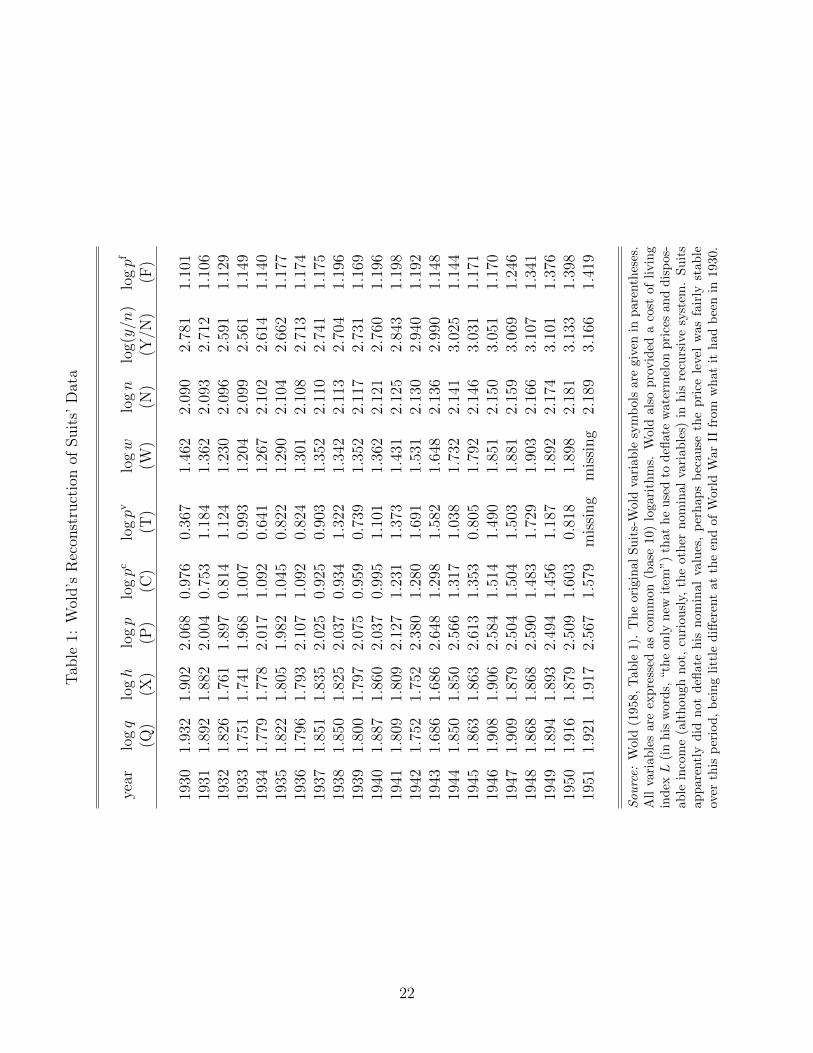
two sets of variable symbols is shown in Table 1.

As in any market for a particular commodity, Suits found that the market for watermelons

has some idiosyncratic features that must be treated. With respect to supply, he found that

it is important to distinguish between a season’s crop of watermelons qt available for harvest,

and the amount ht of that crop actually harvested. Crop supply depends mainly on planting

5

decisions made on information in the previous season:

log qt = α1 + α2 log pt−1 + α3 log pct−1 + α4 log pvt−1 + α5dct + α6d

wt + ε1t. (1)

The variables are:

q crop of watermelons available for harvest (millions)p average farm price of watermelons (dollars per thousand)pc average annual net farm receipts per pound of cotton (dollars)pv average farm price of vegetables, called “commercial truck crops” by Suits (index)dc dummy variable for government cotton acreage allotment program, equals 1 in

1934–51dw dummy variable for World War II, equals 1 in 1943–46

The amount of the crop actually harvested, on the other hand, is dependent on current

farm price pt relative to prevailing farm wages wt, wages being the major cost of harvesting.

(Farm price is the price at the farm gate; that is, the price received by farmers, as opposed

to the retail price paid by consumers. If farm price pt is too low relative to wages wt, farmers

will lose money harvesting the crop. They are better off leaving the melons in the field to

rot.) As well, the harvest ht is of course limited by the available crop qt. Suits therefore

specified harvested supply as

log ht = β1 + β2 log(pt/wt) + β3 log qt + ε2t. (2)

The additional variables are:

h watermelons harvested (millions)w farm wage rates in the South Atlantic States (index)

Turning to the demand side of the market, Suits specified farm price pt as depending on

per capita harvest, ht/nt, per capita income, yt/nt, and transportation costs:

log pt = γ1 + γ2 log(ht/nt) + γ3 log(yt/nt) + γ4 log pft + ε3t. (3)

The additional variables are:

y U.S. disposable incomen U.S. populationpf railway freight costs for watermelons (index)

6

0

100

200

300

400

500

30 32 34 36 38 40 42 44 46 48 50

Price

(a) Price p (dollars per thousand)

40

50

60

70

80

90

30 32 34 36 38 40 42 44 46 48 50

Crop Harvest

(b) Crop q and harvest h (millions)

Figure 1: Watermelon price and quantities, 1930–1951

To summarize, Suits’ model of the watermelon market consists of three equations that

jointly explain crop quantity qt, harvest quantity ht, and price pt. Notice that, setting

aside the dummy variables affecting crop supply, all equations are estimated as loglinear

relations. The original article provides a detailed explanation of the many choices Suits

made in specifying the model. For example, in common with all agricultural commodities

there was a discrete jump in the price of watermelons beginning in 1942, shown in Figure 1a.

The war dummy in crop supply (1) models this as arising from a leftward shift in supply, as

opposed to a rightward shift in demand (3); and indeed the estimate of α6 turns out to be

negative and statistically significant. The intuition is presumably that supply was limited by

a general shortage of factors of production during the war, labor being diverted to the war

effort and land being bid away for other uses. Nevertheless, conditional on the discrete shift

in average price being modeled in this way, price then varies around its pre- and post-1942

mean values in a way that—at least according to the eyeball metric—does not obviously

violate stationarity. (Any more formal analysis of the time series properties of price pt—at

least, any meaningful one—would seem to be precluded by the small sample size.)

As one of the earliest estimated simultaneous equations systems, Suits’ study was influ-

ential in subsequent work. Wold (1958) formulated a modification of the model to illustrate

his famous “causal chain” or “recursive” system, under which the structural form can be

estimated by equation-by-equation OLS. Suits’ model was also used in the forecasting ex-

7

ercise of L’Esperance (1964) and is among the historically important applications discussed

by Wallis (1979). More recently, Murray (2006, 613) cites it as a “golden oldie greatest hit”

piece of empirical work.

But if Suits’ watermelon model was so seminal, why is it now largely forgotten by textbook

writers? Probably because it has a feature that, if treated, introduces enough additional

complication to make it unsuitable as a textbook application. Let us return to the crop

supply and harvest supply equations. Clearly harvest quantity ht is limited by crop quantity

qt, so ht ≤ qt. In most years this constraint is not binding, but in some years (1941–45 and

1948; see the respective columns of Table 1 and their comparison in the plot of Figure 1b) the

crop is fully harvested. Consequently the model has served as an application of econometric

methods for the treatment of truncated variables, being used for this purpose by Goldfeld

and Quandt (1975). It is in this context that the application is discussed by Maddala (1983,

312–315).

But although Suits’ paid careful attention to this aspect of the data, it turns out that

the substantive estimation results are little affected by ignoring it. For the purposes of

student exercises, the model can be estimated using the standard SEM estimators without

incorporating or treating the restriction ht ≤ qt.

Data, estimation, and interpretation

Suits (1955) estimated the equations of his model with annual data using what he describes

as “limited information” methods. From the references he cites, one understands this to

mean limited information maximum likelihood (LIML) rather than two stage least squares

(2SLS). He estimated crop supply for 1919–1951, demand and harvest supply for 1930–51.

However Suits did not publish his data, and when Wold (1958, 22) came to formulate his

recursive system he learned that “. . . Suits had cleared out his files for the original data . . . ”

Wold therefore reconstructed the data for 1930–51, reporting them in his Table 1 (expressed

as common logarithms, with values missing for farm wages and truck crop (vegetable) prices

in the final year 1951). It is Wold’s reconstructed dataset that is provided in my Table 1.

Given the presence of lagged variables in crop supply, this means that the model as a whole

can be estimated for the years 1931–50 using Wold’s data. It is these 20 observations that

8

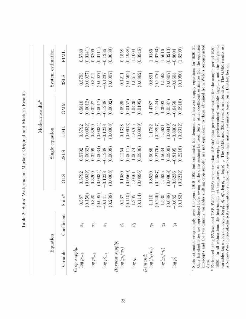
are used to obtain the modern estimation results of Table 2, where they are contrasted with

the results originally reported by Suits. For a statement of the instrument set, see footnote

b of Table 2. The estimation results were obtained with EViews and TSP, cross-checking

between the two to ensure accuracy. (EViews is widely used in teaching, but the numerical

accuracy of TSP’s estimation algorithms has been more favourably assessed (McCullough

1999).)

Despite the reconstruction of the data, the change in sample period for the crop supply

equation, the lack of treatment of the ht ≤ qt constraint, and the primitive computational

technology available to Suits, my estimation results are remarkably similar to his. Equally

surprising is that the modern results are, in terms of the substantive economic interpretations

of coefficient signs, magnitudes, and test outcomes, fairly robust across alternative estimation

methods.

Like great art, Suits’ analysis can be appreciated at several levels of sophistication. This

makes it useful for both introductory and more advanced econometrics courses.

Alternative estimation methods Table 2 reports estimation results for the standard

estimators: OLS, 2SLS, LIML, single-equation GMM, iterative 3SLS, and FIML. The OLS,

2SLS, and LIML estimation results for crop supply are identical because it is a reduced form

equation: the regressors are predetermined (the lagged prices) or exogenous (the dummy

variables). In the case of the harvest supply and demand equations, the similarity of the

OLS and IV-based estimates foreshadows the outcome of Hausman tests on the endogenous

regressors, as we shall see.

The only standard estimator that the application does not admit is system GMM (based

on either a White heteroskedasticity-robust or a Newey-West heteroskedasticity-and-auto-

correlation-robust covariance estimator), because 20 observations is too few to estimate the

system covariance matrix.

Coefficient interpretations and elementary hypothesis tests of fixed-value restric-

tions Suits’ model yields a number of interesting and intuitively sensible elasticities and

simple hypothesis tests that can be appreciated even by beginning students.

9

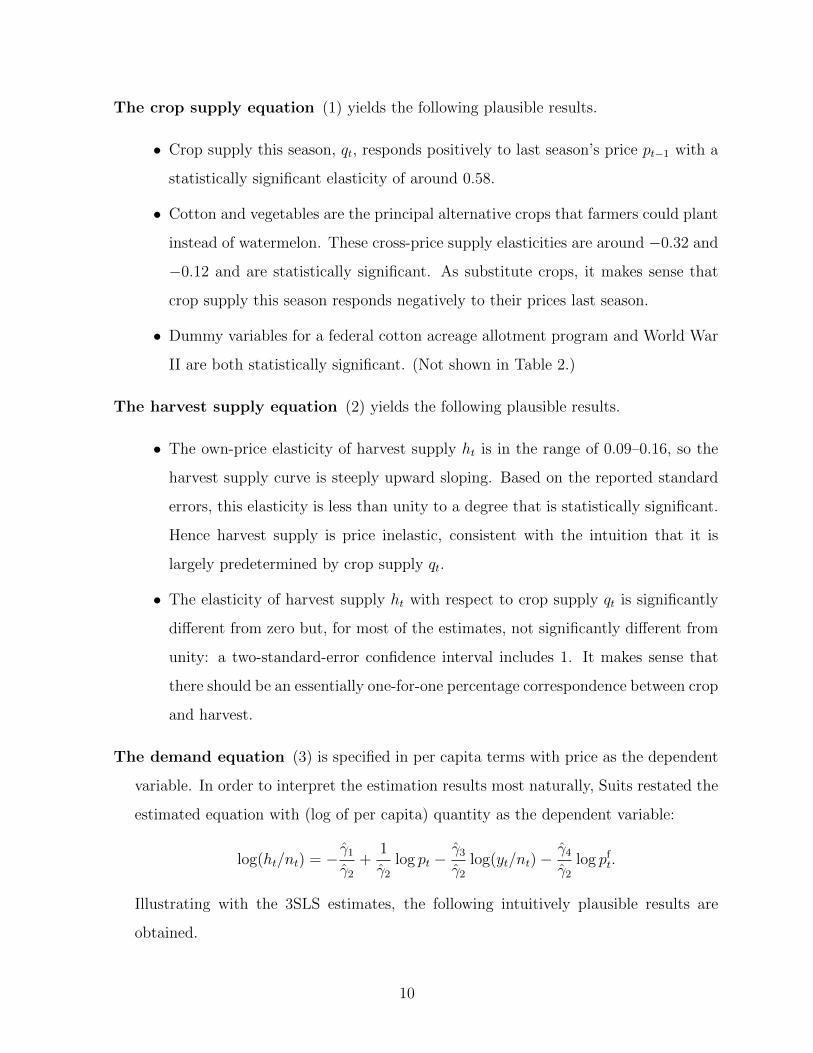
The crop supply equation (1) yields the following plausible results.

• Crop supply this season, qt, responds positively to last season’s price pt−1 with a

statistically significant elasticity of around 0.58.

• Cotton and vegetables are the principal alternative crops that farmers could plant

instead of watermelon. These cross-price supply elasticities are around −0.32 and

−0.12 and are statistically significant. As substitute crops, it makes sense that

crop supply this season responds negatively to their prices last season.

• Dummy variables for a federal cotton acreage allotment program and World War

II are both statistically significant. (Not shown in Table 2.)

The harvest supply equation (2) yields the following plausible results.

• The own-price elasticity of harvest supply ht is in the range of 0.09–0.16, so the

harvest supply curve is steeply upward sloping. Based on the reported standard

errors, this elasticity is less than unity to a degree that is statistically significant.

Hence harvest supply is price inelastic, consistent with the intuition that it is

largely predetermined by crop supply qt.

• The elasticity of harvest supply ht with respect to crop supply qt is significantly

different from zero but, for most of the estimates, not significantly different from

unity: a two-standard-error confidence interval includes 1. It makes sense that

there should be an essentially one-for-one percentage correspondence between crop

and harvest.

The demand equation (3) is specified in per capita terms with price as the dependent

variable. In order to interpret the estimation results most naturally, Suits restated the

estimated equation with (log of per capita) quantity as the dependent variable:

log(ht/nt) = − γ̂1γ̂2

+1

γ̂2log pt −

γ̂3γ̂2

log(yt/nt)−γ̂4γ̂2

log pft.

Illustrating with the 3SLS estimates, the following intuitively plausible results are

obtained.

10

• The own-price elasticity of demand is negative and (in absolute value) less than

unity,1

γ̂2=

1

−0.8891= −1.125, (4)

so watermelon demand is downward sloping and slightly price elastic.

• The income elasticity of demand is positive and greater than unity,

− γ̂3γ̂2

= − 1.5563

−0.8891= 1.750 (5)

so watermelon demand is substantially income elastic, consistent with the intu-

ition that fresh fruit is a luxury to households.

• The cross-price elasticity of demand with respect to freight costs is negative:

− γ̂4γ̂2

= −−0.8604

−0.8891= −0.968. (6)

Ceteris paribus, higher transportation costs shift the demand curve leftward.

Reinterpreted spatially, the implication is the sensible one that, when consumers

are located farther away from growing regions, their demand will be lower than if

they were located closer.

Tests of within-equation linear restrictions The demand and harvest supply equations

specify the regressors log(pt/wt), log(ht/nt), and log(yt/nt) as log-ratios. This is testable.

Specifically, the harvest supply equation (2) is a restricted form of

log ht = β1 + β2 log pt − β∗2 logwt + β3 log qt + ε2t

while watermelon demand (3) is a restricted form of

log pt = γ1 + γ2 log ht − γ∗2 log nt + γ3 log yt − γ∗3 log nt + γ4 log pft + ε3t.

Under the single-equation estimators the restrictions β2 = β∗2 , γ2 = γ∗2 , and γ3 = γ∗3 are

testable individually or, in the case of the latter two, jointly. Under systems estimation all

three can be tested jointly. It is therefore possible to address systematically the question:

Do the data support specifying these regressors as ratios? It also provides an opportunity to

emphasize to students the distinction between individual and joint tests of restrictions, and

that there is no simple relationship between the outcomes of individual versus joint tests.

11

Applications of Wald test routines

A standard device in the toolkit of applied econometricians is the use of Wald test routines

to compute standard errors of nonlinear functions of parameters. Suits’ watermelon model

provides several examples, summarized in Table 3, that range from elementary to more

sophisticated.

Elasticity expressions Consider the nonlinear demand elasticity expressions (4), (5),

and (6). Illustrating with the 3SLS estimates, a Wald test routine yields the standard errors

0.313, 0.496, and 0.360, shown in the first three rows of Table 3. Using these to construct

two-standard-error confidence intervals around their respective demand elasticities reveals

the following conclusions, which are fairly robust across the different estimation methods.

• The own-price elasticity of demand of −1.125 is significantly different from zero, so

watermelon consumption is price elastic, but not significantly different from a unitary

elasticity of −1.

• The income elasticity of demand of 1.750 is significantly different from zero, so water-

melon consumption is income elastic, but not significantly different from unity. The

point estimate is therefore less than compelling in establishing watermelon to be a

luxury.

• The freight elasticity of demand of −0.968 is significantly different from zero, so wa-

termelon consumption is reduced by higher transportation costs.

Dynamic stability Given the presence of lagged price pt−1 in crop supply (1), Suits’

model implies a dynamic path for the evolution of price pt over time. Substituting equations

(1) and (2) into (3), the difference equation governing the evolution of price is of the form

(corresponding to equation (4a) on p. 245 of Suits)

log pt = φ log pt−1 + a function of exogenous variables and disturbances.

12

Stability of the time path of price requires |φ| < 1, which is a testable restriction. The

expression for φ is

φ =γ2β3α2

1− γ2β2. (7)

Illustrating with the 3SLS results reported in the fourth row of Table 3, φ̂ = −0.494 (Suits’

value was −0.622) and a Wald test routine yields a standard error of 0.124, so a two-

standard-error confidence interval around φ̂ does not include |φ| = 1. Hence the estimated

model is consistent with dynamic stability to an extent that is statistically significant, at

least according to the 3SLS estimates. This conclusion is less strongly supported by the

FIML results, where the estimate |φ̂| = 0.560 is within two standard errors of unity.

The half-life of a shock Given the evidence that the estimated model is consistent with

dynamic stability, it is of interest to ask: how long does convergence to equilibrium take?

In the case of a first order difference equation, the standard expression for the half-life of

a shock (which students may have seen in their courses on dynamics) is log(1/2)/ log(|φ|).

Illustrating with the 3SLS results reported in the fifth row of Table 3, this evaluates to

log(1/2)

log(|φ|)=

log(1/2)

log(0.494)= 0.982, (8)

consistent with Suits’ conclusion (p. 426) that “. . . the half life of this process is less than

two years . . . indicating a heavily damped oscillation with rapid approach to equilibrium.”

The standard error of 0.349 suggests that Suits’ conclusion is supported to an extent that is

statistically significant. The FIML evidence is weaker on this point: it yields an estimated

half-life of 1.196 years, but with a larger standard error of 1.268.

Instrumental variables diagnostics

Teachers of IV estimation typically impress on students the scope for testing the implicit

assumptions that underly these methods. Suits’ 1955 study predated modern specification

testing—not just by years, but by decades. How does his analysis stand up to modern

diagnostic tools?

Three categories of IV-related diagnostics are typically discussed by instructors: the

Hansen-Sargan test of the restrictions implied by an overidentifying instrument set; tests of

13

regressor endogeneity; and tests for weak instruments. Table 4 summarizes the results of the

most common of these tests applied to the watermelon model.

Hansen-Sargan tests of overidentification When the instrument set is overidentify-

ing, the “extra” instruments imply a set of parameter restrictions that are testable. The

restrictions should hold as long as the instruments truly are exogenous. Hence a test of the

restrictions can be interpreted as a test of the null hypothesis that the instruments are ex-

ogenous. The associated J statistic was originally proposed by Sargan (1958) in the context

of 2SLS and later extended by Hansen (1982) to GMM.

The top section of Table 4 reports p -values for these tests, which do not reject at conven-

tional significance levels. Hence by this criterion the model and instrument set are broadly

supported.

Hausman tests of regressor endogeneity Is IV estimation really necessary? Only if

the right hand side variables that are specified as endogenous truly are: these are price pt

and crop quantity qt in harvest supply (2), and harvest quantity ht in the demand equation

(3). The endogeneity of these regressors can be tested with Hausman tests, the results of

which are reported in the middle section of Table 4. The large p -values for both equations

indicate that the null hypothesis of exogeneity is not rejected.

This is not terribly surprising for crop quantity qt because, according to the crop sup-

ply equation (1), it is largely determined by information from the previous season. Crop

quantity qt is endogenous only via the correlation between its disturbance ε1t and the other

disturbances of the system.

Exogeneity is more surprising for price pt and harvest quantity ht, which are jointly

determined by the demand and harvest supply equations. This result does explain, however,

why the OLS estimates for these equations are so similar to those yielded by all the IV-based

estimators. A Hausman test essential compares the OLS and IV estimators and asks: are

they significantly different?

Weak instruments Inference with IV-based estimators hinges on their actual finite-

sample distribution being well-approximated by their theoretical asymptotic distribution.

14

For this to be true the instruments should be strongly correlated with the endogenous re-

gressors of an equation.

The simplest indicator of this is the Staiger-Stock F statistic—the F value from the

“first stage” or “reduced form” regression of each 2SLS estimation, in which each of the

endogenous variables is regressed on all the exogenous variables of the system. (I place “first

stage” and “reduced form” in quotations because in a nonlinear model these would not be

the literal interpretations.) The Staiger-Stock rule of thumb is that this F value should be at

least 10 for the exogenous variables to be strong instruments for that endogenous variable.

The bottom row of Table 4 (where each entry corresponds to the endogenous regressor used

as the dependent variable in successive first-stage regressions) indicates that this criterion is

easily satisfied in Suits’ model.

Additional empirical issues

In addition to the results discussed so far, Suits’ model provides the opportunity to expose

students to several minor but nevertheless important practical issues.

Issues related to the use of logarithms In introductory econometrics courses students

learn that in a log-log regression the coefficients are interpretable as elasticities, while in a

log-lin model—like a regression of log wages on education—the coefficient is a semielasticity:

multiplied by 100, it is the percentage change in the dependent variable (like wages) associ-

ated with a unit change in the explanatory variable (like an additional year of schooling).

A more obscure point, but one that Wold’s data provides instructors the opportunity

to comment on, is the extent to which these interpretations are affected by the base of the

logarithm. The elasticity interpretation is not: Wold’s dataset is in common logarithms, but

the results of a log-log regression are invariant to this, and the estimates of Table 2 are the

same elasticities (and standard errors) that would be obtained were the data in natural logs.

In contrast, the semielasticity interpretation assumes natural logs. For example, consider the

war dummy in crop supply (1). The 3SLS estimate of its coefficient (not shown in Table 2)

is α̂6 = −0.1567 with a standard error of 0.0008, indicating that World War II significantly

reduced crop supply. However the correct interpretation is not that this reduction was in

15

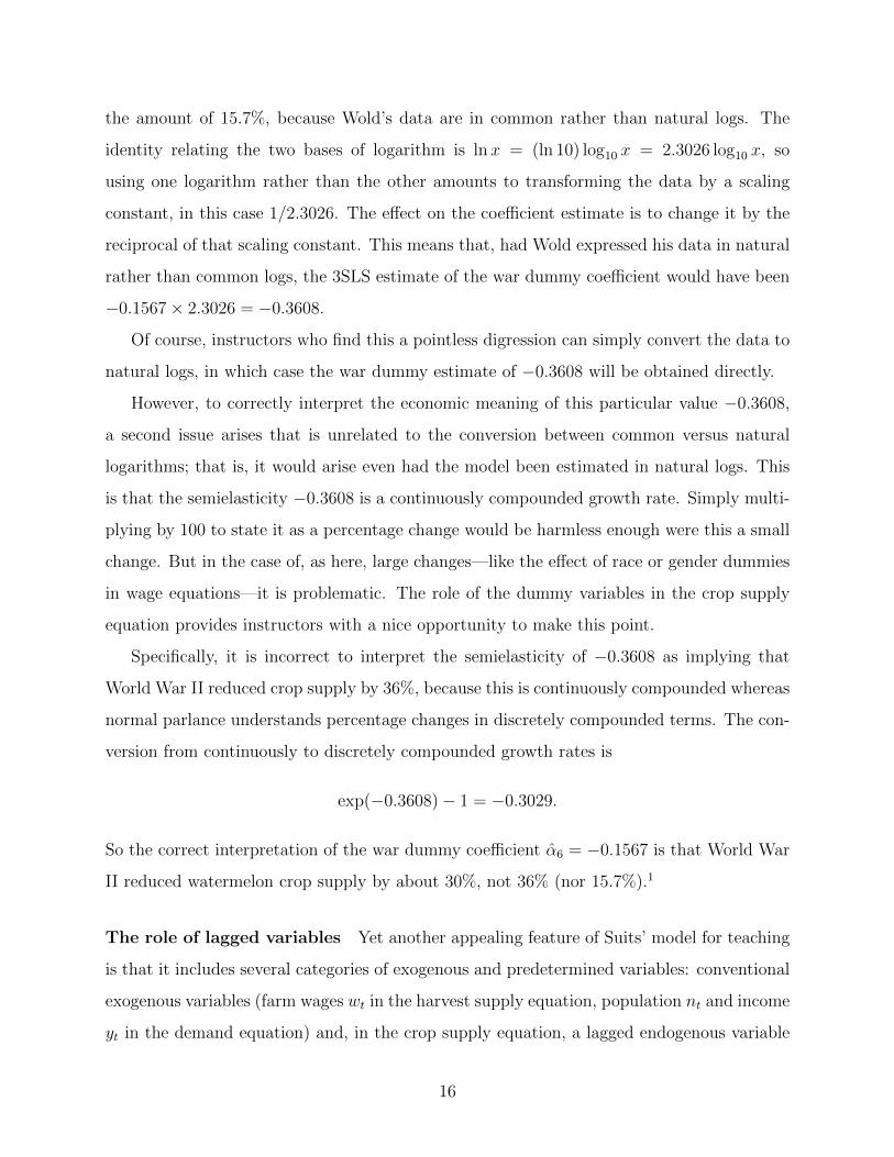
the amount of 15.7%, because Wold’s data are in common rather than natural logs. The

identity relating the two bases of logarithm is lnx = (ln 10) log10 x = 2.3026 log10 x, so

using one logarithm rather than the other amounts to transforming the data by a scaling

constant, in this case 1/2.3026. The effect on the coefficient estimate is to change it by the

reciprocal of that scaling constant. This means that, had Wold expressed his data in natural

rather than common logs, the 3SLS estimate of the war dummy coefficient would have been

−0.1567× 2.3026 = −0.3608.

Of course, instructors who find this a pointless digression can simply convert the data to

natural logs, in which case the war dummy estimate of −0.3608 will be obtained directly.

However, to correctly interpret the economic meaning of this particular value −0.3608,

a second issue arises that is unrelated to the conversion between common versus natural

logarithms; that is, it would arise even had the model been estimated in natural logs. This

is that the semielasticity −0.3608 is a continuously compounded growth rate. Simply multi-

plying by 100 to state it as a percentage change would be harmless enough were this a small

change. But in the case of, as here, large changes—like the effect of race or gender dummies

in wage equations—it is problematic. The role of the dummy variables in the crop supply

equation provides instructors with a nice opportunity to make this point.

Specifically, it is incorrect to interpret the semielasticity of −0.3608 as implying that

World War II reduced crop supply by 36%, because this is continuously compounded whereas

normal parlance understands percentage changes in discretely compounded terms. The con-

version from continuously to discretely compounded growth rates is

exp(−0.3608)− 1 = −0.3029.

So the correct interpretation of the war dummy coefficient α̂6 = −0.1567 is that World War

II reduced watermelon crop supply by about 30%, not 36% (nor 15.7%).1

The role of lagged variables Yet another appealing feature of Suits’ model for teaching

is that it includes several categories of exogenous and predetermined variables: conventional

exogenous variables (farm wages wt in the harvest supply equation, population nt and income

yt in the demand equation) and, in the crop supply equation, a lagged endogenous variable

16

(watermelon price pt−1), lagged exogenous variables (the prices pct−1 and pvt−1), and dummy

variables (dct , dwt ). Let us call these eight variables the default instrument set. It is useful for

students to see—as few textbook examples allow them to—that all these types of variables

can appear in a SEM and may serve as instruments.

The modern estimation results of Tables 2–4 follow Suits (as best I have been able to

determine) in using this default instrument set. But the waters here run deep and, depending

on the student audience, some instructors may wish to explore them.

Specifically, issues of both identification and estimation potentially arise in connection

with some of these variable categories, questions that go back to the earliest work on SEMs

and, in some cases, continue to this day. Sims (1980, 5) usefully summarized some of the

early literature:

J.D. Sargan several years ago considered the problem of simultaneous-equation

identification in models containing both lagged dependent variables and serially

correlated residuals. He came to the reassuring conclusion that, if a few narrow-

looking special cases are ruled out, the usual rules for checking identification in

models with serially uncorrelated residuals apply equally well to models with

serially correlated residuals. In particular, it would ordinarily be reasonable to

lump lagged dependent variables with strictly exogenous variables in checking

the order condition for identification, despite the fact that a consistent estima-

tion method must take account of the presence of correlation between the lagged

dependent variables and the serially correlated residuals.

. . . work by Michio Hatanaka, however, makes it clear that this sanguine con-

clusion rests on the supposition that exact lag lengths and orders of serial corre-

lation are known a priori. On the evidently more reasonable assumption that lag

lengths and shapes of lag distributions are not known a priori, Hatanaka shows

that the order condition takes on an altered form: we must in this case cease

to count repeat occurrences of the same variable, with different lags, in a single

equation. In effect, this rule prevents lagged dependent variables from playing

the same kind of formal role as strictly exogenous variables in identification . . .

17

The Sargan-Hatanaka controversy by no means exhausts the issues that arise in con-

nection with the role of lagged variables in SEMs. For a recent contribution with a useful

bibliography, see Reed (2015).

For pedagogical purposes the point is merely that, for the minority of instructors who

wish to explore these issues, Suits’ model offers scope for doing so. For the majority who

prefer to circumvent them, as I have in Tables 2–4, this is easily and probably harmlessly

done.

Pedagogical deficiencies

Are there any deficiencies of Suits’ model as an example of SEM methodology? Two come

to mind.

System GMM cannot be implemented because there is an inadequate number of obser-

vations to estimate the system covariance matrix (under either a White heteroskedasticity-

robust or Newey-West heteroskedasticity-and-autocorrelation-robust specification).

Limited role for cross-equation restrictions Instructors often cite efficiency as the

motivation for system estimation as an alternative to single-equation estimation, with the

caveat that efficiency improvements are conditional on the model being correctly specified.

Although this logic is correct, in practice the more important reason for system estimation

is often the desire to impose and test cross-equation restrictions.

A limitation of Suits’ model for pedagogical purposes is that the scope for this is modest,

arising only tangentially in connection with the dynamic stability expression (7) and the

half-life (8). Because these involve coefficients from both the demand and harvest supply

equations, obtaining standard errors for them requires system estimation, as the construction

of Table 3 emphasizes.

For instructors seeking an empirical application in which the role of cross-equation re-

strictions is more central, a better choice might be a system of demand equations—either

consumer or factor demands—because the cross-equation restrictions of symmetry are pre-

dicted by microeconomic theory and can be imposed and tested. For example, Berndt (1991)

18

provides the data, including the instruments, needed to replicate the 3SLS translog factor de-

mand system of Berndt and Wood (1975). Of course, this assumes a background in demand

analysis that goes beyond what undergraduates usually see. The appeal of Suits’ model is

that it yields economically interpretable results that are interesting and intuitive, yet can be

understood with only the most elementary background in economics.

Conclusions

I have advanced Suits’ watermelon model as an almost ideal simultaneous equations empirical

application for instructors who want an example that goes beyond the typical textbook two-

equation model. Among its many strengths are the following.

• It falls within the classic simultaneous equations paradigm of supply and demand for an

agricultural commodity, in which each equation stands on its own as a ceteris paribus

behavioral relation.

• It is of some historical importance, in terms of being seminal at the time and influential

in subsequent work.

• It is based on a well-documented real-world data set of modest size that is easily

disseminated to and used by students.

• It yields interesting and intuitive results that are readily interpretable in terms of

elementary economic theory.

• It provides scope for a range of interesting hypothesis tests, confidence intervals, and the

use of Wald test routines to obtain standard errors for nonlinear coefficient expressions.

• It provides a vehicle for discussing a variety of minor but nevertheless important prac-

tical issues, such as the use of log transformations, the interpretation of dummy coef-

ficients, and the role of lagged variables in identification, estimation, and dynamics.

• Although it uses time series data over 20 years, conventional SEM analysis can rea-

sonably be regarded as not being contaminated by a failure to treat nonstationarity.

19

Finally, Suits’ watermelon model is an empirical application that pays tribute to the

early development of the SEM, one of the few econometric methodologies that advances

fundamentally beyond statistics proper.

Notes

1These are the issues that Suits refers to in his footnote 2 by way of explanation for hisconclusion (p. 241) that “. . . wartime policy clearly reduced the supply of melons signifi-cantly, the size of the parameter corresponding to a reduction of 30 percent.” The correctinterpretation of dummy coefficients in log-lin regressions is well known among empiricallabor economists, because it so often arises in that context. Curiously, it is seldom discussedin econometrics textbooks.

References

Angrist, J., and J.-S. Pischke. 2017. Undergraduate econometrics instruction: Through

our classes, darkly. Journal of Economic Perspectives 31: 125–144.

Berndt, E.R. 1991. The Practice of Econometrics: Classic and Contemporary. Addison-

Wesley.

Berndt, E.R., and D.O. Wood. 1975. Technology, prices, and the derived demand for

energy. Review of Economics and Statistics 57: 259–268.

Dougherty, C. 2016. Introduction to Econometrics, 5th Edition. Oxford University Press.

Goldfeld, S., and R. Quandt. 1975. Estimation in a disequilibrium model and the value of

information. Journal of Econometrics 3: 325–348.

Gujarati, D., and D. Porter. 2009. Basic Econometrics, 5th Edition. McGraw-Hill.

Hansen, L. 1982. Large sample properties of generalized method of moments estimators.

Econometrica 50: 1029–1054.

Kennedy, P. 2008. A Guide to Econometrics, 6th Edition. Blackwell Publishing.

L’Esperance, W. 1964. A case study in prediction: The market for watermelons. Econo-

metrica 32: 163–173.

20

Maddala, G. 1983. Limited-Dependent and Qualitative Variables in Econometrics. McGraw-

Hill.

McCullough, B.D. 1999. Econometric software reliability: EViews, LIMDEP, SHAZAM,

and TSP. Journal of Applied Econometrics 14: 191–202.

Murray, M. 2006. Econometrics: A Modern Introduction. Pearson: Addison-Wesley.

Reed, W. 2015. On the practice of lagging variables to avoid simultaneity. Oxford Bulletin

of Economics and Statistics 77: 897–905.

Sargan, D. 1958. The estimation of economic relationships using instrumental variables.

Econometrica 26, 393–415.

Sims, C. 1980. Macroeconomics and reality. Econometrica 48: 1–48.

Stock, R., and M. Watson. 2015. Introduction to Econometrics, 3rd Edition. Pearson.

Studenmund, A. 2017. Using Econometrics: A Practical Guide, 7th Edition. Pearson.

Suits, D. 1955. An econometric model of the watermelon market. Journal of Farm Eco-

nomics 37: 237–251.

Wallis, K. 1979. Topics in Applied Econometrics, 2nd ed. Blackwell Publishing.

Wold, H. 1958. A case study of interdependent versus causal chain systems. Review of the

International Statistical Institute 26: 5–25.

Wooldridge, J. 2016. Introductory Econometrics: A Modern Approach, 6th Edition. Cen-

gage Learning.

21

Tab

le1:

Wol

d’s

Rec

onst

ruct

ion

ofSuit

s’D

ata

year

logq

logh

logp

logpc

logpv

logw

logn

log(y/n

)lo

gpf

(Q)

(X)

(P)

(C)

(T)

(W)

(N)

(Y/N

)(F

)

1930

1.93

21.

902

2.06

80.

976

0.36

71.

462

2.09

02.

781

1.10

119

311.

892

1.88

22.

004

0.75

31.

184

1.36

22.

093

2.71

21.

106

1932

1.82

61.

761

1.89

70.

814

1.12

41.

230

2.09

62.

591

1.12

919

331.

751

1.74

11.

968

1.00

70.

993

1.20

42.

099

2.56

11.

149

1934

1.77

91.

778

2.01

71.

092

0.64

11.

267

2.10

22.

614

1.14

019

351.

822

1.80

51.

982

1.04

50.

822

1.29

02.

104

2.66

21.

177

1936

1.79

61.

793

2.10

71.

092

0.82

41.

301

2.10

82.

713

1.17

419

371.

851

1.83

52.

025

0.92

50.

903

1.35

22.

110

2.74

11.

175

1938

1.85

01.

825

2.03

70.

934

1.32

21.

342

2.11

32.

704

1.19

619

391.

800

1.79

72.

075

0.95

90.

739

1.35

22.

117

2.73

11.

169

1940

1.88

71.

860

2.03

70.

995

1.10

11.

362

2.12

12.

760

1.19

619

411.

809

1.80

92.

127

1.23

11.

373

1.43

12.

125

2.84

31.

198

1942

1.75

21.

752

2.38

01.

280

1.69

11.

531

2.13

02.

940

1.19

219

431.

686

1.68

62.

648

1.29

81.

582

1.64

82.

136

2.99

01.

148

1944

1.85

01.

850

2.56

61.

317

1.03

81.

732

2.14

13.

025

1.14

419

451.

863

1.86

32.

613

1.35

30.

805

1.79

22.

146

3.03

11.

171

1946

1.90

81.

906

2.58

41.

514

1.49

01.

851

2.15

03.

051

1.17

019

471.

909

1.87

92.

504

1.50

41.

503

1.88

12.

159

3.06

91.

246

1948

1.86

81.

868

2.59

01.

483

1.72

91.

903

2.16

63.

107

1.34

119

491.

894

1.89

32.

494

1.45

61.

187

1.89

22.

174

3.10

11.

376

1950

1.91

61.

879

2.50

91.

603

0.81

81.

898

2.18

13.

133

1.39

819

511.

921

1.91

72.

567

1.57

9m

issi

ng

mis

sing

2.18

93.

166

1.41

9

Source:

Wol

d(1

958,

Tab

le1).

Th

eori

gin

al

Su

its-

Wold

vari

ab

lesy

mb

ols

are

giv

enin

pare

nth

eses

.A

llva

riab

les

are

exp

ress

edas

com

mon

(base

10)

logari

thm

s.W

old

als

op

rovid

eda

cost

of

livin

gin

dex

L(i

nh

isw

ord

s,“th

eon

lyn

ewit

em”)

that

he

use

dto

defl

ate

wate

rmel

on

pri

ces

an

dd

isp

os-

able

inco

me

(alt

hou

ghn

ot,

curi

ou

sly,

the

oth

ern

om

inal

vari

ab

les)

inh

isre

curs

ive

syst

em.

Su

its

app

aren

tly

did

not

defl

ate

his

nom

inal

valu

es,

per

hap

sb

ecause

the

pri

cele

vel

was

fair

lyst

ab

leov

erth

isp

erio

d,

bei

ng

litt

led

iffer

ent

at

the

end

of

Worl

dW

ar

IIfr

om

wh

at

ith

ad

bee

nin

1930.

22

Tab

le2:

Suit

s’W

ater

mel

onM

arke

t:O

rigi

nal

and

Moder

nR

esult

s

Moder

nre

sult

sb

Equat

ion

Sin

gle

equat

ion

Syst

emes

tim

atio

n

Var

iable

Coeffi

cien

tSuit

saO

LS

2SL

SL

IML

GM

M3S

LS

FIM

L

Cropsupp

ly:

logp t

−1

α2

0.58

70.

5792

0.57

920.

5792

0.58

100.

5793

0.57

89(0

.156

)(0

.003

2)(0

.003

2)(0

.003

2)(0

.001

2)(0

.002

7)(0

.014

1)lo

gpc t−

1α3

−0.

320−

0.32

09−

0.32

09−

0.32

09−

0.32

27−

0.32

12−

0.32

09(0

.095

)(0

.003

4)(0

.003

4)(0

.003

4)(0

.001

7)(0

.002

7)(0

.011

1)lo

gpv t−

1α4

−0.

141−

0.12

38−

0.12

38−

0.12

38−

0.12

38−

0.12

37−

0.12

36(0

.238

)(0

.000

8)(0

.000

8)(0

.000

8)(0

.000

2)(0

.000

7)(0

.003

9)Harvest

supp

ly:

log(p

t/w

t)β2

0.23

70.

1080

0.12

540.

1328

0.09

250.

1211

0.15

58(0

.110

)(0

.056

9)(0

.061

1)(0

.061

3)(0

.015

7)(0

.056

2)(0

.193

8)lo

gq t

β3

1.20

51.

0461

1.06

741.

0765

1.04

291.

0617

1.10

04(0

.114

)(0

.089

6)(0

.093

6)(0

.093

9)(0

.019

5)(0

.086

2)(0

.394

6)Dem

and:

log(h

t/nt)

γ2

−1.

110−

0.85

20−

0.90

86−

1.17

82−

1.47

87−

0.88

91−

1.01

85(0

.246

)(0

.268

7)(0

.277

6)(0

.289

7)(0

.122

4)(0

.247

6)(0

.670

3)lo

g(y

t/nt)

γ3

1.53

01.

5635

1.56

341.

5631

1.39

931.

5563

1.56

16(0

.088

)(0

.090

8)(0

.090

9)(0

.094

9)(0

.058

7)(0

.080

7)(0

.321

3)lo

gpf t

γ4

−0.

682−

0.82

36−

0.81

95−

0.80

02−

0.64

58−

0.86

04−

0.86

04(0

.183

)(0

.221

2)(0

.221

6)(0

.231

2)(0

.091

0)(0

.195

0)(1

.629

9)

aS

uit

ses

tim

ated

crop

sup

ply

over

the

years

1919–1951

bu

tes

tim

ate

dh

isd

eman

dan

dh

arv

est

sup

ply

equ

ati

on

sfo

r1930–51.

On

lyh

isel

asti

citi

esar

ere

pro

du

ced

her

e;ow

ing

toth

ed

ata

scali

ngs

he

use

d,

Su

its’

oth

erco

effici

ent

esti

mate

s(f

or

the

equ

ati

on

inte

rcep

tsan

dth

etw

od

um

my

vari

ab

les

shif

tin

gcr

op

sup

ply

)are

not

equ

ivale

nt

toth

ose

ob

tain

edfr

om

Wold

’sre

con

stru

cted

dat

a.b

Est

imat

edu

sin

gE

Vie

ws

and

TS

P.

Wold

’s(1

958)

reco

nst

ruct

ion

of

Su

its’

data

per

mit

ses

tim

ati

on

for

the

sam

ple

per

iod

1930–

1950

.In

all

esti

mat

ion

sth

ein

stru

men

tse

tco

mp

rise

san

inte

rcep

t,th

ep

red

eter

min

edva

riab

lelo

gpt−

1,

an

dth

eex

ogen

ou

sva

riab

les

logw

t,

lognt,

logy t

,lo

gpf t,dc t,dw t

,lo

gpc t−

1,

logpv t−

1.

Th

eG

MM

an

d3S

LS

resu

lts

are

iter

ati

ve.

Th

eG

MM

resu

lts

use

aN

ewey

-Wes

th

eter

oske

das

tici

ty-a

nd

-au

toco

rrel

ati

on

-rob

ust

cova

rian

cem

atr

ixes

tim

ato

rb

ase

don

aB

art

lett

ker

nel

.

23

Tab

le3:

Use

ofW

ald

Tes

tR

outi

nes

toC

ompute

Sta

ndar

dE

rror

sfo

rN

onlinea

rE

xpre

ssio

ns

Expre

ssio

n2S

LS

LIM

LG

MM

3SL

SF

IML

own-p

rice

elas

tici

tyof

dem

and

1/γ2

−1.

101−

0.84

9−

0.67

6−

1.12

5−

0.98

2(0

.336

)(0

.209

)(0

.056

)(0

.313

)(0

.646

)in

com

eel

asti

city

ofdem

and

−γ3/γ

21.

721

1.32

70.

946

1.75

01.

533

(0.5

36)

(0.3

36)

(0.0

98)

(0.4

96)

(1.1

15)

frei

ght

cros

s-pri

ceel

asti

city

ofdem

and

−γ4/γ

2−

0.90

2−

0.67

9−

0.43

7−

0.96

8−

0.84

5(0

.384

)(0

.269

)(0

.079

)(0

.360

)(1

.841

)dynam

icst

abilit

yφ

=γ2β3α2/(

1−γ2β2)

−0.

494−

0.56

0(0

.124

)(0

.344

)hal

f-life

log(1/2

)/lo

g(|φ|)

0.98

21.

196

(0.3

49)

(1.2

68)

24

Table 4: Instrumental Variables Diagnostics

Equation Crop supply Harvest supply DemandDependent variable log q log h log p

Instrument exogeneity:a (p -values)2SLS Sargan J test 0.319 0.719 0.110GMM Hansen J test 0.612 0.865 0.714

Endogenous regressors:b (p -values)Hausman test using 2SLS residuals 0.707 0.425

Weak instruments:c

Staiger-Stock first-stage F statistic 7680.08 24.06 168.46

a The null hypothesis is that the restrictions implied by the overidentifying instrument set aresatisfied. Rejection indicates misspecification.

b The null hypothesis is that the regressors specified as endogenous are actually exogenous,implying that IV estimation is unnecessay. Rejection indicates endogeneity, suggesting thatIV estimation is desirable. There is no Hausman test for crop supply because that equationhas no endogenous regressors.

c These are the F statistics from OLS regressions of each endogenous variable (log q, log h, log p)on the instrument set. A Staiger-Stock F value less than 10 is a rule-of-thumb indicator ofweak instruments.

25