00 (2015) 1–23

JournalLogo

www.elsevier.com/locate/procedia

The Multi-Depot Split-Delivery Vehicle Routing Problem:Model and Solution Algorithm

Sujoy Raya, Andrei Soeanua, Jean Bergerb, Mourad Debbabia

aConcordia University, Montreal, Quebec, CanadabDefence R&D Canada - Valcartier, Quebec, Canada

Abstract

Logistics and supply-chain management may generate notable operational cost savings with increased reliance on shared

serving of customer demands by multiple agents. However, traditional logistics planning exhibits an intrinsic limitation

in modeling and implementing shared commodity delivery from multiple depots using multiple agents. In this paper, we

investigate a centralized model and a heuristic algorithm for solving the multi-depot logistics delivery problem including

depot selection and shared commodity delivery. The contribution of the paper is threefold. First, we elaborate a new

integer linear programming (ILP) model, namely: Multi-Depot Split-Delivery Vehicle Routing Problem (MDSDVRP)

which allows establishing depot locations and routes for serving customer demands within the same objective function.

Second, we illustrate a fast heuristic algorithm leveraging knowledge gathering in order to find near-optimal solutions.

Finally, we provide performance results of the proposed approach by analyzing known problem instances from different

VRP problem classes. The experimental results show that the proposed algorithm exhibits very good performance when

solving small and medium size problem instances and reasonable performance for larger instances.

© 2013 Published by Elsevier Ltd.

Keywords: Multi-Depot Vehicle Routing Problem, Integer Linear Programming, Heuristic Algorithm, Supply Chain

Management, Operations Research, etc.

1. Introduction

The technological transformations that are taking place over the last few decades have brought about

new challenges to the conventional supply chain operations in organizations ranging from private enter-

prises to governmental institutions. The changing global economy and agile infrastructure have placed high

demand for systematic and automated planning of large-scale commodity delivery operations. In this re-

spect, academic and industrial research and development efforts are being pursued for logistics operational

plan generation. In this article, we intend to explore a subset of such large-scale planning requirements

and analyze how multiple distribution centers (depots) and vehicle routing paths can be derived together,

if possible, in a centralized planning environment to deliver commodities within predefined constraints and

limited vehicle capacity. The specific focus of this study is the multi-depot split-delivery and location rout-

ing problem. The proposed technique can efficiently compute near-optimal solutions for problem instances

where the combined cost (distribution center establishment and vehicle routing) needs to be minimized.

2 Author / 00 (2015) 1–23

1.1. Motivation & BackgroundBusiness organizations address their logistics pursuits at three different levels. These levels are often

referred as: Strategic, Operational and Tactical [1]. Strategically, decision makers locate depots for serving

the customers. Various network partitioning and resource allocation algorithms are applied on external

inputs to choose depot locations in the vicinity of the customers. Once the depots are chosen, operational

decision makers solve the underlying routing problem as per the requirements. The problem types at this

level are often characterized as: traveling salesman problem (TSP), vehicle routing problem (VRP), traveling

repairman problem (TRP), etc. Analytical, heuristic and meta-heuristic algorithms are used to solve the

routing problems where the typical objective is to minimize routing cost. The results of these planning

processes are a set of vehicle routes. Finally, the tactical officers proceed to execute the routing tasks in

compliance with previously taken decisions. The need for large-scale quick logistic delivery planning is

vital for situations like humanitarian aid distribution, disaster relief, rescue operations and national crises.

However, such a multi-level decision making exhibits notable gaps to find optimal partitioning and routing

in the transportation network for commodity delivery [2]. Furthermore, traditional logistics planning and its

subsequent execution phase(s) heavily depend on human expertise in decision making that exhibit intrinsic

limitations in handling large and complex operations. In this respect, an efficient and sufficiently automated

mechanism for sharing responsibilities in commodity delivery may offer better situational response.

A relevant situation can be mentioned from the experience of the well-known Haiti disaster in the after-

math of the January 2010 earthquake [3]. In this crisis situation, the response operations started the delivery

of essential commodities to more than 300,000 injured and 1.5 million homeless people [3]. Several organi-

zations, such as: International Rescue Committee (IRC), Management Sciences for Health (MSH), Interna-

tional Federation of Red Cross (IFRC), etc., teamed up to deliver drugs and supplies to out-of-stock clinics

and health facilities from multiple operational Emergency Response Units1. It was well documented that the

overwhelming emergency requirements caused delay in shelter preparation [3]. Renowned news channels

also reported on the mismanagement in cooperation for shared delivery arrangement among participating

organizations2. The logistics delivery planning is also an important research problem for the supply chain

management. In the commercial sectors, trade related surface transportation has been constantly increasing

in North America. Between 2009 and 2010, the total value-added of the Transportation and Warehousing

sector has been growing approximately by 4.3% [4]. In Canada, the Gross Domestic Product (GDP) in the

Transportation and Warehousing sector has increased from $50.2 billion in 2001 to $58.4 billion in 2010 [4].

The United States Department of Transportation has issued a notable report stating that the surface trans-

portation trade between North American Free Trade Agreement (NAFTA) partners has been increased by

11.5% in January 2012 compared to January 2011 at $75.5 billion [5]. Alongside, a Gartner report reveals

that the market for intelligent transportation planning software holds the key to the success of the multi-

organizational response. The report also indicates a 20.6% increase of worldwide Transport Management

System software revenue from 2007 ($538 million) to 2008 ($648 million) and a growth in the field through

2012 (up to $963 million) [6].

1.2. Problem ElaborationMulti-Depot Split-Delivery Vehicle Routing Problem (MDSDVRP) handles commodity delivery to cus-

tomers (demand points) that are represented as nodes in a complete graph named as transport network.

Given a set of nodes (V) and a set of edges (E), where E is a relation in (V × V), a transport network is a

complete graph G = (V,E). Each edge of the graph provides the traversal cost (ci j) between the correspond-

ing two nodes i and j. Usually, a transport network is composed of different node types: Customers (N) and

Depots (D). While customer nodes are characterized with deterministic demand (integer) for commodity

(δi), depot nodes (having no demand) alternatively host vehicles (k = 1,2, . . .K) to supply customers. In

case of predefined depots and customers, a solution for an MDSDVRP instance gives the routes for each

vehicle that minimizes the overall routing cost to serve all customer demands. In our proposed formulation,

1MSH and IRC to Partner in Haiti; link: http://www.msh.org/news-bureau/msh-and-irc-to-partner-in-haiti.cfm2BBC, What is delaying Haiti’s aid?; link: http://news.bbc.co.uk/2/hi/americas/8472670.stm

Author / 00 (2015) 1–23 3

we further consider that if the depots are not predefined, the solution to MDSDVRP will determine the

optimal location(s) of the depot(s) within the set of customer nodes. In this case, assuming that the newly

found depot(s) will serve their own need(s), the goal of problem is then to minimize the combined depot

establishment and routing cost.

In actuality, vehicle routing can be seen as a core problem in supply chain/logistics planning, with con-

ceptual, empirical and behavioral aspects. A holistic view of the supply chain process offers an overarching

perspective spanning over various facets such as facility location, vehicle routing and environmental impact.

In this respect, focusing on a single aspect, for example minimizing the routing cost without considering

facility locations may result in higher warehousing cost and larger externalities such as: pollution, conges-

tion, etc. In the usual setup, the problem of multi-depot split delivery vehicle routing is considered with the

common assumptions of Split-Delivery VRP (SDVRP) and Multi-Depot VRP (MDVRP) under which we

essentially consider a vehicle routing problem involving commodity delivery as an abstract conceptual op-

timization problem [7] with few empirical details. The participating entities are depots (as starting/ending

points for vehicles), customers (with deterministic demand) and vehicles (with predefined and available

capacity). Typical abstractions are observed in terms of unlimited route length (not considering required

stop-overs for rest, etc.) as well as deterministic infrastructure analysis (fixed traversal cost across transport

network nodes, etc.). Another prevalent abstraction is to consider the problem of facility location separate

as specifically employed by cluster first-route second approaches [2]. However, in this work, we emphasize

the importance of considering together the problems of location allocation and vehicle routing.

The optimization goal of VRP is the overall cost minimization based on the cost assigned on each

edge of the transportation network. In the literature the deterministic capacitated-VRP (CVRP) is a well-

studied NP-hard combinatorial optimization problem having several variants and extensions [8]. In fact, the

CVRP is composed of two problems: Bin-Packing and Routing. The Bin Packing Problem (BPP) addresses

an optimal allocation of commodity to vehicles having deterministic capacity. The routing problem deals

with the most efficient routing possible using the loaded vehicles. We may note that in shared commodity

delivery settings (which represent practical aspects at the requirements level), it is possible to determine the

feasibility of a problem instance by requiring the total vehicle capacity to be greater or equal to the total

demand. In other words, MDSDVRP will always yield a solution if the total available capacity is equal

or more than the total demand. In this respect, MDSDVRP is less restrictive than some of the other VRP

variants for which there may be no feasible solution (e.g some customers having demands larger than the

capacity of a single vehicle). However, MDSDVRP still belongs to the NP-hard class of problems [9, 10]

and is therefore intractable when approached with an exact algorithm. It is worthy to mention that it has a

notable larger solution space since splitting the delivery among different vehicles is subject to combinatorial

explosion. Consequently, we detail an effective heuristic technique that yields good near-optimal solutions.

1.3. Objectives

In the scope of this article, we aim at investigating an advanced decision support platform to address

a combined problem of depot assignment and logistics delivery planning. Currently available transport

management systems exhibit notable gaps in optimal partitioning of transport network for shared delivery of

logistics/commodities [6]. In order to bridge the gap, we introduce a linear model of the combined problem

and propose a generic solution search technique for multi-depot vehicle routing problems that may employ

shared delivery of commodities, if needed. The solutions to this problem is expected to efficiently use a

number of vehicles of predefined capacity to serve geographically distant customers of known demands.

The objectives of this paper can be summarized as follows:

• Elaborate an ILP model to find locations for the depots and the vehicle routes of commodity delivery.

• Propose an efficient fast-convergent heuristic-based mechanism to solve the model near-optimally.

• Generate solution benchmarks for known problem instances and compare with existing results.

• Analyze the performance and provide other notable insights of the proposed solution.

4 Author / 00 (2015) 1–23

The core contribution of this paper includes the elaboration of an integer linear programming (ILP) op-

timization model for multi-depot, multi-vehicle per depot vehicle routing with split delivery. A notable

contribution relates to the flexibility of the proposed model. This allows to customize it via small modifi-

cations (according to the need) in order to address specific problems of the VRP family that are within the

scope of the proposed model. These include MDVRP (no split delivery), SDVRP (only one depot), CVRP

(no split delivery and only one depot), etc. Moreover, the concept of location routing allows to consider

both location allocation and vehicle routing as part of the same objective function. In this context, it is also

possible to customize the depot establishment cost values such as to predefine depots at specific locations.

With respect to the related heuristics algorithm, it allows to generate vehicle routes with near-optimal cost

while serving the customers by multiple vehicles belonging to the same or different depots.

1.4. Article Organization

The remainder of the paper is organized as follows. Section 2 offers an overview of the related work

on various types of vehicle routing problems. Section 3 elaborates the proposed model for MDSDVRP and

our solution generation approach. It describes a generic heuristic based searching mechanism designed to

solve vehicle routing problem instances, MDSDVRP instances in particular. Along with the algorithm, we

also discuss two improvement techniques over the initially derived solutions. Section 4 presents a relevant

case study problem illustrating CVRP, MDVRP and MDSDVRP in order to demonstrate solution generation

using the proposed approach. In Section 5, we provide the results and compare them to existing benchmark

values. We further conduct an analysis of the results in Section 6 to determine appropriate ranges for

the parameter values used in the solution approach. Finally, we summarize our findings in Section 7 by

highlighting the benefits and the limitations of the proposed procedure and conclude with future work.

2. Related Work

The transportation management and logistics delivery problems are known for their practical relevance

and high computational complexity. They have been extensively studied across the scientific community

all around the world for more than half a century. Many of these problems commonly exhibit NP-hard

complexity and are often modeled from centralized perspective. In the literature, there are different research

articles discussing multi-stage approaches to solve logistics delivery planning. Numerous research initiatives

propose multi-stage approaches [1, 8] that require network partitioning and choosing the facility locations

at the first stage. Then, in the latter stage, they consider various VRP variants to deliver commodities.

The transport network partitioning problem belongs to the more general graph partitioning problem

whose objective is to partition a graph into approximately equal parts with the least number of intercon-

nections. The graph partitioning problem is known to be NP-complete [11]. Thus, there is no general

tractable procedure that would allow to efficiently perform optimal graph partitioning for large problem in-

stances. Nonetheless, specific approaches allow for graph partitioning in geographical information systems,

telecommunication networks, clustering, image processing and many other areas [12, 13, 14], including

operations research. Jarrah and Bard published a heuristic approach [15] for graph partitioning using con-

tiguous geographic clustering for pickup and delivery VRP via network route segmentation. Many algo-

rithms addressing network partitioning exist in the literature, such as: K-Means clustering [16], DB-Scan

algorithm, shortest path algorithm [17] etc. However, the underlying limitations of the “cluster-first, route-

second" approaches stems from the fact that the best depot locations obtained by partitioning at the strategic

level may not always optimize the cost at the operational level since the depot locations are generally chosen

without considering the potential routing cost. Salhi and Rand [2] show that the best solution after facility

location stage does not necessarily lead to the lowest cost solution after the routing stage.

VRP aims at commodity delivery to a set of customers by a set of vehicles, from one or many depots

over a transport network characterized by a full mesh graph. Early on, Dantzig and Ramser [18] formally

introduced the vehicle routing problem in their pioneering work on truck dispatching. VRP entails combi-

natorial optimization to reach optimal routing cost solution. In 2002, Toth and Vigo elaborated an extensive

classification of VRP family [8]. Subsequently, Golden et al. documented the more recent advancements

Author / 00 (2015) 1–23 5

of the last decade in [19]. In this article, we focus on capacitated-VRP (CVRP). In its original form, CVRP

includes the bin packing problem, which need to be solved along with the routing in order to optimally use

the available capacity of the vehicles and optimally serve the customers. CVRP is usually expressed as a

linear optimization problem with several constraints represented through linear equations and inequalities.

Three commonly used CVRP models include the Vehicle Flow Model, Commodity Flow Model and Set

Partitioning Model [8]. SDVRP is related to CVRP as it aims at minimizing the total traveling cost for

commodity delivery but it allows to serve individual customer demands by more than one vehicle. SD-

VRP instances observe relaxed bin-packing constraints and a feasible solution always exists if the overall

customer demand is less or equal to the overall capacity available. The concept of split-delivery was first

introduced by Dror and Trudeau [20] and later further elaborated by Archetti and Speranza [21]. A sur-

vey on the progress in SDVRP has been recently published by Archetti et al. [22] where the benefits of

shared delivery are illustrated on various problem instances. However, an important limitation of SDVRP

lies in the availability of a single depot. In this article, we take the problem of SDVRP into our MDSD-

VRP model, which is addressing in addition the depot location allocation problem while allowing vehicles

from the same or different depots to participate in shared commodity delivery. In the proposed MDSDVRP

model, we employ split-delivery vehicle routing and also address facility location by choosing depots from

a subset of customer nodes (based on their corresponding depot establishment cost). The model also allows

the use of pre-established depots by setting the corresponding depot establishing cost to zero. Toward this

end, we incorporate idea from the Location Routing Problem (LRP) [1] which combines location allocation

and vehicle routing. This involves determining depots and routes for a fixed number of vehicles to serve

customers. Although LRP definition is elaborated, it suffers from traditional key limitation that the set of

candidate depots is generally pre-established. In our previous work, we presented the concept of MDSDVRP

by extending the aforementioned ideas [23].

Recently, Gulczynski et al. [10] investigated a version of MDSDVRP by extending SDVRP. Their work

relates to our problem to some extent. The authors provide a mixed integer programming optimization model

that is essentially addressing route cost minimization by applying split delivery among vehicles from the

same or different depots. However, the employed approach is multi-stage as it considers first the assignment

of customers to depots using a distance based approximation, solving then the split-delivery VRP for each

depot. Thereafter, further improvements are pursued by creating inter depot routes. The authors combine a

mixed integer programming with a variable length record-to-record travel algorithm for which experimental

results shows the cost reduction from splitting the deliveries among vehicles from different depots. However,

the work has a number of limitations as follows. First, it employs an apriori, rule-based allocation of

customers to depots by favoring the assignment to the nearest depots. In case of insufficient vehicle capacity,

this will lead to a higher cost. Such concerns were addressed in [24] where a distant depot is required to

serve a customer that is closest to another depot in order to achieve overall cost reduction. Second, the

proposed solving technique leverages the Clarke and Wright (CW) saving mechanism that is limited in

its applicability to the situations where the triangle inequality is satisfied [25]. Furthermore, the model

considers only predefined depot locations on the transport network.

VRPs represent a well studied class of NP-hard problems [8]. Traditional (analytical) solving tech-

niques such as branch and bound [19], are intractable for medium and large scale problems. Therefore,

solution generation often involves various supervised solution searching procedures such as: heuristic and

meta-heuristic algorithms which are commonly used to find near-optimal solutions for NP hard problems

[26]. Concerning customer allocation, Chan and Kumar [27] developed ant-colony based meta-heuristic

optimization for managing customer demands whereas Zhou et al. [28] used a genetic algorithm based ap-

proach for customers allocation to their distribution center. Heuristics and mathematical programming for

cargo loading are studied in [26] and [29]. In the case of SDVRP, Archetti et al. showed that the SDVRP

can be solved in polynomial time if and only if common vehicle capacity (C) is 2 [22] whereas the problem

becomes NP-hard for C > 2. Dror et al. described a local search algorithm based on specific SDVRP prop-

erties [30]. Archetti et al. obtained improved results using Tabu search [21]. Chen et al. proposed a hybrid

algorithm, additionally using the standard Clarke and Wright saving algorithm in order to solve SDVRP.

In the context of logistics planning for natural disasters, Ozdamar et al. presented an approach of

planning in emergency situation [31]. Yi and Kumar also used an ant colony based approach for optimizing

6 Author / 00 (2015) 1–23

disaster relief operations [32]. In the case of MDSDVRP, we opted for near-optimal solution generation

using heuristic procedures. Heuristic methodologies usually involve a directed search procedure based on

knowledge gathering. Meta-heuristics, generally involves comparing and iteratively enhancing candidate

solutions with respect to a defined quality function measure. In our research context, generational heuristic

algorithms followed by solution refinements are more suitable especially to address adaptive route planning.

A preliminary version of our proposed heuristic algorithm has been introduced in [33].

3. Proposed Approach

In the following, we present an overview of the approach to solve the aforementioned research problem.

Under a set of assumptions, we propose an ILP model for the multi-depot vehicle routing problem allowing

joint serving of customer demands using vehicles from multiple depots. The model allows to identify the

problem requirements in terms of variables and parameters. However, MDSDVRP belongs to the problem

class NP-hard [10]. Therefore, no scalable exact solution algorithm exists to efficiently find the optimal

solution. Consequently, we investigate a heuristic algorithm that can efficiently explore a large portion of

the solution space in order to find a good near-optimal solution. The proposed search procedure is guided

by a learning mechanism that allows to steer the search toward the most probable area of the solution space

where near optimal solutions are likely to be found. We also employ a stochastic technique to prevent the

premature convergence of the algorithm to a local optimal solution.

3.1. Assumptions

Classical VRP generally refers to the capacitated vehicle routing problem (CVRP) where each location

(customer) has a finite demand (integer value) for the same type of commodity. A maximum number of

vehicles having finite capacity (integer value) can start from and return to a single depot, with no restriction

on the route length. In addition, each location is served by only one vehicle and the sum of the demands

served by a vehicle does not exceed the vehicle capacity. It is also customarily assumed that the vehicle fleet

is homogeneous, that is all vehicles have the same capacity. Moreover, MDVRP changes the assumption

of a single depot and considers the availability of more than one depot, each of which can serve any of the

customers. In this setup it is also customarily assumed that the vehicle fleet is homogeneous across depots

(the same maximum number of homogeneous vehicles). Capacitated VRP with split delivery (SDVRP)

shares most assumptions of CVRP except that each customer can be served by one or more vehicles that

jointly satisfy the total customer demand. This allows to address problems where the individual capacity of

the vehicles can be less than some (or all) of the customer demands. MDSDVRP combines the assumptions

of MDVRP with those of SDVRP such that each customer can be served by one or more vehicles, each of

which can belong to the same or different depots. In addition to the aforementioned constraints, we intend

to address the situation where there is are no pre-established depot(s) in the problem. The depots locations

are then chosen from the set of customer locations. Consequently, the demands at the node locations chosen

as depot locations are considered to be served by the respective depot itself. In order to solve the problem,

the heuristic procedure may be exercised by one or more decision maker(s). The corresponding MDSDVRP

solution algorithm assumes that all input information is exact. We assume that each decision maker has the

knowledge of all available vehicles in every depot along with their capacities. S/he also knows the cost of

routing across every edge of the transport network. In case of more than one decision maker, we consider

the existence of a centralized result sharing platform where multiple decision makers can share information

while searching a partially different solution space.

3.2. MDSDVRP Modeling

In a complete directed graph G = (V,E) of a transport network, let ci j be an input cost matrix derived

from a composed cost function (depending on various parameters) for all node pairs. We extend this trans-

port network graph G to G′ = (V ′,E′) wherein an arbitrary node 0 is added in the transport graph such

that V ′ = V ∪ {0}. The concept was earlier introduced by Yu et al. [34]. The intent of including node

0 as a virtual node is to carefully capture the facility (depot) location subproblem as a part of the routing

Author / 00 (2015) 1–23 7

0

A B

C D

2.4

2.1

2.2

1.1

1.4

1.2

1.3;2.3

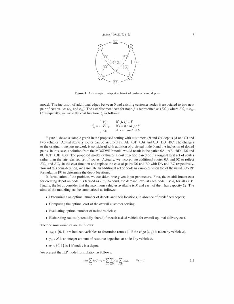
Figure 1: An example transport network of customers and depots

model. The inclusion of additional edges between 0 and existing customer nodes is associated to two new

pair of cost values (ci0 and c0 j). The establishment cost for node j is represented as (EC j) where EC j = c0 j.

Consequently, we write the cost function c′i j as follows:

c′i j =

⎧⎪⎪⎪⎨⎪⎪⎪⎩

ci j if {i, j} ⊂ VEC j if i = 0 and j ∈ Vci0 if j = 0 and i ∈ V

Figure 1 shows a sample graph in the proposed setting with customers (B and D), depots (A and C) and

two vehicles. Actual delivery routes can be assumed as: AB�BD�DA and CD�DB�BC. The changes

to the original transport network is considered with addition of a virtual node 0 and the inclusion of dotted

paths. In this case, a solution from the MDSDVRP model would result in the paths: 0A�AB�BD�D0 and

0C�CD�DB�B0. The proposed model evaluates a cost function based on its original first set of routes

rather than the later derived set of routes. Actually, we incorporate additional routes 0A and 0C to reflect

ECA and ECC in the cost function and replace the cost of paths D0 and B0 with DA and BC respectively.

Toward this consideration, we associate an additional set of boolean variables wi on top of the usual SDVRP

formulation [9] to determine the depot locations.

In formulation of the problem, we consider three given input parameters. First, the establishment cost

for creating depot on node i is termed as ECi. Second, the demand level at each node i is: di for all i ∈ V .

Finally, the let us consider that the maximum vehicles available is K and each of them has capacity Ck. The

aims of the modeling can be summarized as follows:

• Determining an optimal number of depots and their locations, in absence of predefined depots;

• Computing the optimal cost of the overall customer serving;

• Evaluating optimal number of tasked vehicles;

• Elaborating routes (potentially shared) for each tasked vehicle for overall optimal delivery cost.

The decision variables are as follows:

• xi jk ∈ {0,1} are boolean variables to determine routes (1 if the edge (i, j) is taken by vehicle k).

• yik ∈ N is an integer amount of resource deposited at node i by vehicle k.

• wi ∈ {0,1} is 1 if node i is a depot.

We present the ILP model formulation as follows:

min∑i∈V

ECiwi +∑i∈V∑j∈V

ci j∑k∈K

xi jk, ∀i ≠ j (1)

8 Author / 00 (2015) 1–23

Subject to:

Flow conservation:

∑i∈V′∑k∈K

xi jk ≥ 1, ∀ j ∈ V ′, i ≠ j (2)

∑j∈V∑k∈K

x0 jk ≤ ∣K∣ (3)

x0ik = xi0k ∀i ∈ V and k ∈ K (4)

∑i∈V′

xipk = ∑j∈V′

xp jk ∀p ∈ V ′and k ∈ K, i, j ≠ p (5)

Sub-tour elimination:

∑i∈S∑j∈S

xi jk −∑j∈S

x0 jk ≤ ∣S ∣ − 1, S ⊆ V, ∣S ∣ ≥ 2, k ∈ K and i ≠ j (6)

Capacity restriction:

∑i∈V

yik ≤ Ck, ∀k ∈ K (7)

∑k∈K

yik = di(1 −wi), ∀i ∈ V (8)

yik ≤ di ∑j∈V′

xi jk, ∀i ∈ V and k ∈ K (9)

Depot assignment:

∑k∈K

x0ik ≥ wi, ∀i ∈ V (10)

x0ik ≤ wi, ∀i ∈ V, k ∈ K (11)

Variables:

xi jk ∈ {0,1}; where i, j ∈ V ′, i ≠ j, k ∈ K (12)

wi ∈ {0,1}; where i ∈ V (13)

yik ≥ 0; where i ∈ V, i ≠ j, k ∈ K (14)

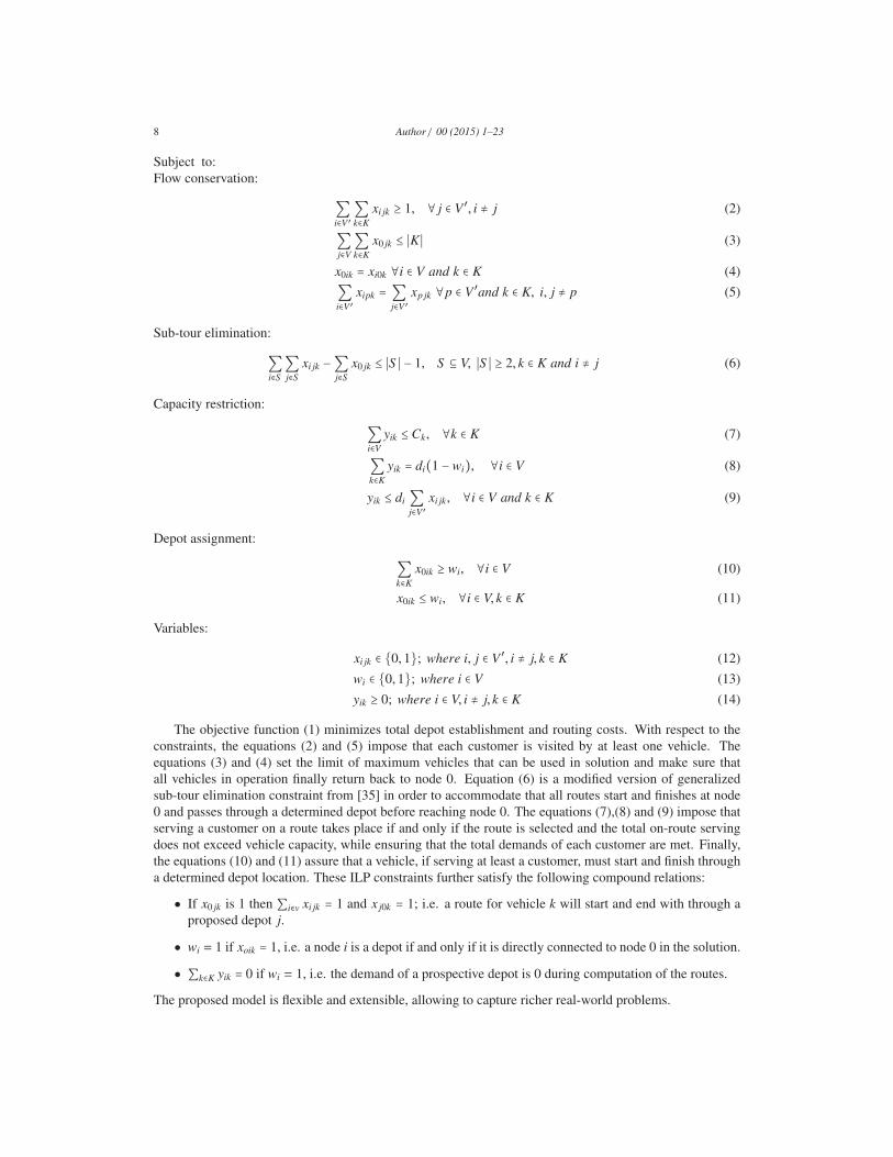
The objective function (1) minimizes total depot establishment and routing costs. With respect to the

constraints, the equations (2) and (5) impose that each customer is visited by at least one vehicle. The

equations (3) and (4) set the limit of maximum vehicles that can be used in solution and make sure that

all vehicles in operation finally return back to node 0. Equation (6) is a modified version of generalized

sub-tour elimination constraint from [35] in order to accommodate that all routes start and finishes at node

0 and passes through a determined depot before reaching node 0. The equations (7),(8) and (9) impose that

serving a customer on a route takes place if and only if the route is selected and the total on-route serving

does not exceed vehicle capacity, while ensuring that the total demands of each customer are met. Finally,

the equations (10) and (11) assure that a vehicle, if serving at least a customer, must start and finish through

a determined depot location. These ILP constraints further satisfy the following compound relations:

• If x0 jk is 1 then ∑i∈v xi jk = 1 and x j0k = 1; i.e. a route for vehicle k will start and end with through a

proposed depot j.

• wi = 1 if xoik = 1, i.e. a node i is a depot if and only if it is directly connected to node 0 in the solution.

• ∑k∈K yik = 0 if wi = 1, i.e. the demand of a prospective depot is 0 during computation of the routes.

The proposed model is flexible and extensible, allowing to capture richer real-world problems.

Author / 00 (2015) 1–23 9

• MDSDVRP can be tailored to select pre-established depots by suitably choosing low establishment

cost for some favored nodes and high establishment cost for others (see Table 4).

• With many vehicles and one depot in configuration, this model may express an SDVRP.

• One can provide product or service through the same model. For simplicity, we assume that service

delivery (e.g. surveillance) resembles product delivery but the vehicle capacity (Ck) is not reduced

after visiting the demand nodes. However it must meet the service requirements (yik). Thus, we

change Equation (7) as follows:

yik ≤ Ck, ∀k ∈ K and ∀i ∈ V (15)

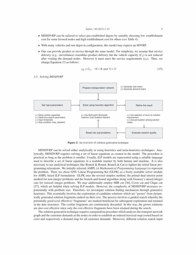
3.3. Solving MDSDVRP

Solve using heuristic algorithm

Prepare transportation network

Set input parameters Refine the result

Evaluate solution qualityBreak into sub-problems

(+) Use Multi-point StochasticInsertion Cost Gradient Descent

(+) Setup vehicle capacities(+) Determine search parameters(+) Input thresholds(+) Stop condition (max_iteration)

(+) Generate cost-matrix(+) Generate demand-matrix

(+) Use selection of tours for solutionimprovement(+) Use permutation among solutionnodes

Figure 2: An overview of solution generation technique

MDSDVRP can be solved either analytically or using heuristics and meta-heuristics techniques. Ana-

lytically, MDSDVRP requires solving a set of linear equations as created in the model. The procedure is

practical as long as the problem is smaller. Usually, ILP models are represented using a suitable language

used to describe a set of linear equations in a readable manner by both human and machine. It is also

necessary to use analytical techniques like Branch & Bound, Branch & Cut to tighten the initial linear pro-

gramming relaxations. We initially selected AMPL (A Mathematical Programming Language) to represent

the problem. Then, we chose GNU Linear Programming Kit (GLPK) as a freely available solver module

for AMPL based ILP formulation. GLPK uses the revised simplex method, the primal-dual interior point

method for non-integer problems and the branch-and-bound algorithm along with Gomory’s mixed integer

cuts for (mixed) integer problems. We may additionally employ MIR cut [36], Cover cut and Clique cut

[37], which are helpful when solving ILP models. However, the complexity of MDSDVRP increases ex-

ponentially with problem size. Therefore, we investigate solution finding mechanism through generative

heuristics. This essentially involves the exploration of candidate solutions which are “grown" from dynam-

ically generated solution fragments ranked on their cost. The process involves a guided search whereby the

potentially good (cost effective) “fragments" are marked beneficial for subsequent exploration and retained

in the data structures. The costlier fragments are continuously discarded. In this way, the grown solutions

are also cost effective since only the cost effective fragments have been retained during the search.

The solution generation technique requires a preparation procedure which analyzes the transport network

graph and the customer demands at the nodes in order to establish an ordered traversal map (sorted based on

cost) and respectively a demand map for all customer demands. Moreover, different solution search input

10 Author / 00 (2015) 1–23

parameters are also required to be set before the algorithm run. After a careful analysis on various heuristic

algorithms, we arrived at a modified multi-point stochastic insertion cost gradient descent algorithm to

address solution search from multiple depots. The search allows the insertion of customer nodes in the

explored set of route fragments, subsequently boosting the more cost effective set of routes iteratively.

Figure 2 presents the solution generation approach which assures that a ready solution is always avail-

able after the first pass. The algorithm is also expected to help in cooperative solving of compound routing

problems by a team of potentially remotely located agents. In this setting, during the search process, pro-

gressively better upper bounds found by different agents can be exchanged for improved convergence. The

heuristic solution can be further improved using meta-heuristic like techniques such as permutation of ad-

jacent nodes in routes, etc. Also, the approach allows the use of a divide and conquer policy in order to

handle large scale problems whereby sub-problems involving a subset of the routes will be subjected to the

same algorithm with the potential to yield better overall results. In the following, we discuss the details of

the multi-point stochastic insertion cost gradient descent algorithm.

3.4. Algorithm Design

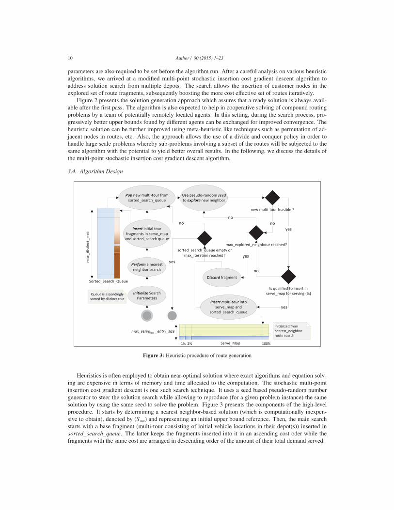
Figure 3: Heuristic procedure of route generation

Heuristics is often employed to obtain near-optimal solution where exact algorithms and equation solv-

ing are expensive in terms of memory and time allocated to the computation. The stochastic multi-point

insertion cost gradient descent is one such search technique. It uses a seed based pseudo-random number

generator to steer the solution search while allowing to reproduce (for a given problem instance) the same

solution by using the same seed to solve the problem. Figure 3 presents the components of the high-level

procedure. It starts by determining a nearest neighbor-based solution (which is computationally inexpen-

sive to obtain), denoted by (S nn) and representing an initial upper bound reference. Then, the main search

starts with a base fragment (multi-tour consisting of initial vehicle locations in their depot(s)) inserted in

sorted_search_queue. The latter keeps the fragments inserted into it in an ascending cost oder while the

fragments with the same cost are arranged in descending order of the amount of their total demand served.

Author / 00 (2015) 1–23 11

Algorithm 1 : MDSDVRP Heuristics

1: Input: max_iteration,S nn,max_distinct_cost(mdc),max_explored_neighbor(maxnbr),2: max_servemap_entry_size(msset), init_ f ragment, seed,usesplit3: Global Knowledge: transport_network_graph(G),demand_map(dmap)4: Output: S ∗

5: Initialize: S ∗ ← S nn; sorted_search_queue(sque) ← ∅; servemap ← {}; D∗ ← GetAllDemand(dmap);6: Insert(init_ f ragment, sque);

7: while max_iteration ≥ 0 and sque is not empty do8: pop MultiTour s from top of sque;

9: if s contains more than one tour then10: Use Shuffle(seed) to randomize their order;

11: end if12: for selectedTour in s do13: Find next customer: nextDst ← GetNextCustomer(G,LastInsertedElementOf(selectedTour));

14: maxNN ← maxnbr;

15: while maxNN > 0 and CountDistinctCostEntries(sque) ≤ mdc do16: Find demand to be served: nextS erveNeed ← GetDemandOf(nextDst, dmap);

17: if nextS erveNeed > 0 then18: if usesplit or nextS erveNeed ≤ GetRemainingCapacity(selectedTour) then19: InsertInTour(nextDst, selectedTour) ;

20: end if21: if CostOf(s) > CostOf(S ∗) then22: continue;

23: end if24: if GetServeAmt(s) = D∗ or GetRemainingCapacity(s) = 0 then25: S ∗ ← s;

26: Remove each multi-tour(s′) fragments from sque where CostOf(s′) > CostOf(s);

27: end if28: if SizeOf(GetEntry(GetServeAmt(s),servemap)) < msset or

CostOf(s) ≤ GetMaxValueIn(GetEntry(GetServeAmt((s),servemap)) then29: Insert(CostOf(s), GetEntry(GetServeAmt(s), servemap));

30: Insert(s, sque);31: end if32: if SizeOf(serveset(GetServeAmt(s)))> msset then33: RemoveMaxValueIn(GetEntry(GetServeAmt(s),servemap));

34: end if35: end if36: maxNN ← maxNN - 1;

37: end while38: end for39: max_iteration← max_iteration - 1;

40: end while41: return S ∗;

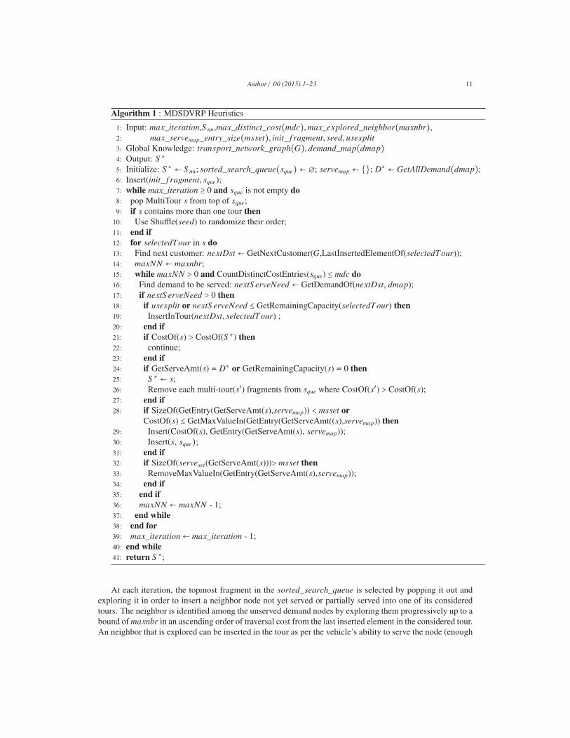
At each iteration, the topmost fragment in the sorted_search_queue is selected by popping it out and

exploring it in order to insert a neighbor node not yet served or partially served into one of its considered

tours. The neighbor is identified among the unserved demand nodes by exploring them progressively up to a

bound of maxnbr in an ascending order of traversal cost from the last inserted element in the considered tour.

An neighbor that is explored can be inserted in the tour as per the vehicle’s ability to serve the node (enough

12 Author / 00 (2015) 1–23

remaining capacity when split delivery is not used or non-empty capacity otherwise). After inserting the

neighbor in the selected fragment, the latter is updated with a corresponding increased cost of serving and

increased amount of serving. The updated fragment is then qualified for storing in the sorted_search_queueby examining if its cost of serving fits within the bounds of the corresponding servemap entry. The servemap

data structure is essentially employed to build up and represent the knowledge related to the specific topology

and serving availability characterizing the problem instance being solved. The knowledge gathered is rep-

resented by a set of adjustable cost bounds corresponding to particular percentages of total demand serving

as discovered during fragment generation. This knowledge is used to continuously guide the search proce-

dure by qualifying or disqualifying potential fragments while they are being explored. Thus, the servemap

keeps entries related to the cost of serving at each related serving percentage (granularity dependent). Each

entry holds a set of different cost values (for the same serving percentage) with a maximum cardinality of

max_servemap_entry_size. A qualified fragment will update the corresponding servemap entry.

During solution search, the servemap entries are populated by progressively smaller cost bounds in as-

cending order of cost. When the maximum entry size is reached, the highest value is removed from the

entry set updating the knowledge related to serving the corresponding percentage of total demand. This in

turn places tighter selection pressure on subsequently explored fragments with the same serving amount.

The fragments placed in the sorted_search_queue are stored until the max_distinct_cost bound is reached.

Subsequently, a fragment is discarded if its updated cost is higher than the maximum cost value of the

stored fragments. When a fragment is updated such that is forms a complete solution, any member of

sorted_search_queue that has a higher cost can be removed since a complete solution with lower cost has

been found. The procedure continues as long as the sorted_search_queue is not empty and alongside pro-

gressively lower cost complete solutions can be identified, with the one having the lowest cost remaining

as the final result of solution search. The effectiveness of this solution generation procedure stems from

the following. First, the heuristic employs an evolving selection pressure to identify better quality frag-

ments leveraging knowledge gathering based on the corresponding cost values stored in the servemap. The

fragments selected in this manner are potentially more able to eventually develop good near-optimal so-

lutions. Second, the procedure exhibits a thorough local search characteristic since all the fragments in

sorted_search_queue are explored and updated according to their cost. Finally, the gradual solution gener-

ation trajectory leverages bounded local neighbor exploration which allows for faster convergence.

Algorithm 1 elaborates in pseudo-code the aforementioned concept by extending our previous work

[33]. We describe next the notation used for the input parameters and the output. An upper bound solution

denoted by S nn provides an initial reference that can be quickly determined using the nearest neighbor.

A demand map (dmap) holds the demands of each node. The sorted_search_queue is an ascendantly

sorted queue of solution fragments based on the cost. The servemap represents an associative array used

for knowledge gathering where each entry contains an ordered set (of parameterized maximum cardinality -

max_servemap_entry_size) containing fragment serving cost values corresponding to a related percentage of

total serving. Seed (seed) represents a unique number used to generate repeatable (for the same seed value)

pseudo-random choices. The maximum number of neighbors to be considered in fragment exploration is

represented by maxnbr. The usesplit is a binary input that selects whether the heuristic algorithm considers

split-delivery. The algorithm is presented at a high level of abstraction with self explanatory names for the

called procedures which follow the convention of having the first letter capitalized.

3.5. Property AnalysisHeuristic algorithms provide practical means to approximately solve optimization problems in short

time and bounded memory with a trade-off in solution quality [38]. Moreover, specific challenges are faced

during an extensive assessment of the properties characterizing heuristic algorithms. In this respect, our

technique has a similar profile. Thus, in the scope of this paper, we provide three important insights with

respect to the termination, convergence and solution quality.

• Termination: Every execution of MDSDVRP heuristic will eventually stop.

• Convergence: Any execution of MDSDVRP heuristic for a feasible problem will converge toward acompetitive solution if the search is not stopped by the maximum iteration count.

Author / 00 (2015) 1–23 13

• Solution quality: The solution found by executing the MDSDVRP heuristic represents the lowest localoptimal within the scope of the solution search space delineated by the underlying search parameters.

With respect to the first property, every selected multi-tour fragment is restricted to explore only within a

set of customer nodes that are among the closest unserved (or partially served) maxnbr neighbors. Therefore,

for a feasible problem, the search procedure only evaluates and stores distinct fragments that can grow at

most to full solutions (all customers fully served). In this respect, the fragment exploration procedure either

reduces (eventually down to 0) the remaining demand unserved or discards the disqualified fragments. Since

the solution space of MDSDVRP is finite, albeit potentially very large, at the extreme (for a sufficiently large

values of the search parameters), the algorithm will stop after an exhaustive evaluation of all competitive

solutions within the search space. However, with reasonable parameter values, the heuristic will only search

a subset of the solution space, bounded in memory and time.

Concerning the second property, given the dynamics of the search technique, the potentially promising

multi-tours will evolve similarly, (with respect to their granularity based serving percentage) before growing

to a full solution. This growth characteristic is stemming from the fact that the serve_map restricts the

storage of multi-tour fragments over a cost bounded percentage of serving and the sorted_search_queuestores the multi-tours in an ascending order of serving cost. Therefore, for each subsequent solution found,

the probability of finding a better solution within a fixed delineated search space decreases successively

and the solution improvement margin follows a natural logarithmic path. Figure 9 depicts the convergence

characteristic (see Section 6). Our analysis on various problem instances reveals empirically that the solution

cost (y) convergence curve over time (t) can be approximated as: y = −C1 × ln(t) +C2, (C1, C2 are positive

constants) with Pearson Coefficient of Determination (R2) value of a few percentage points under unity.

Finally, the algorithm handles premature convergence by competitively ranking different potentially

promising multi-tours based on their cost. The corresponding fragments are qualified by the bounds main-

tained in serve_map according to the percentage of serving. In essence, serve_map supports a guided learn-

ing over the heuristic procedure in order to promote the growth of potentially good multi-tour fragments

from diverse exploration points within evolving tightness bounds. This guidance benefits the multi-point

gradient descent such that each of the growing multi-tours leads toward a local optimal solution bounded by

the search constraints. Therefore, the final solution emerges as the lowest one among all the local optimal

solutions, generated from the diversely explored multi-tours.

3.6. Refinement Technique

The initial heuristic technique we introduced in [33] included solution refinement techniques for improv-

ing the routing cost, including localized node permutation and a Density Based Clustering tour refinement.

The latter was used to dynamically generate traversal cost (distance equivalent) clusters over vehicle tour

nodes. This was aimed at inter-dependent route identification using incremental clustering distances over

related complete solution tour pairs until all nodes of a tour belong to the same cluster. Then, if any node

(except for directly density connected ones) binds two otherwise separate clusters, then the two tours are

likely to allow for solution improvement by solving the corresponding sub-problem. Thus, better (lower

cost) routing is likely to be identified if available. In this work, we retain the localized node permutation

refinement and introduce an alternate (more scalable) non-deterministic tour delineated sub-problem refine-

ment. Both of these refinements are detailed next. We employ the following schemes in order to locally

improve the heuristic solution as follows:

• Selective Localized Permutation Refinement: We generate node permutations (up to a predefined

threshold) around adjacent tour nodes trying to obtain a lower routing cost in the scope of a given

vehicle tour. The permutation procedure is continued successively around adjacent neighbors until no

further gain can be achieved.

• Non-deterministic tour delineated sub-problem refinement: we proceed to non-deterministically de-

lineate tour pairs for iterative improvement by selecting for successive iterations only those that lead

to cost saving along with all the other pairs that share a member with one of the tours improved in the

14 Author / 00 (2015) 1–23

current iteration. This way, better solution can be progressively identified while reducing the number

of tour pairs selected for further improvement over multiple iterations until no further cost savings

can be obtained.

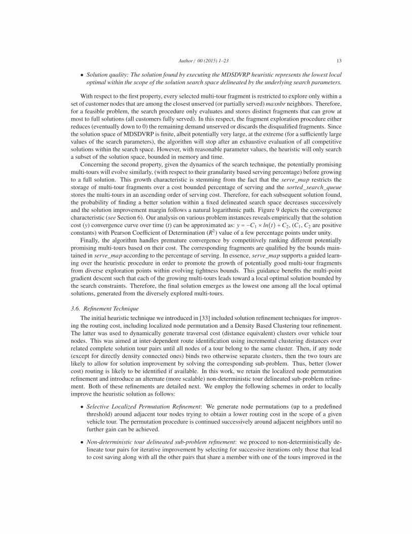
4. Case Study

In this section, we apply the proposed algorithms on a running example of a transport network in various

experimental setups. The selected problem is modified from the original CVRP problem instance: (E016-

03m) as published by Golden et al. [39]. The configuration of the transport network and customer demand

of this new problem are presented below.

Figure 4: Transport network and customer demands

Node X Y Demand EC

1 300 400 0 0

2 370 520 7 0

3 490 490 30 0

4 520 640 16 1000

5 200 260 9 1000

6 400 300 21 1000

7 210 470 15 1000

8 170 630 19 1000

9 310 620 23 1000

10 520 330 11 1000

11 510 210 5 1000

12 420 410 19 1000

13 310 320 29 1000

14 50 250 23 1000

15 120 420 21 1000

16 360 160 10 1000

Table 1: Problem Instance Data

Figure 4 presents the example problem in a 2-Dimensional Euclidean graph. The customer nodes and their

demands are presented in the format of ([node no.]:[serving]). We formed the problem such that the depots

may use at most two vehicles. All of them have capacity of delivering 90 units of commodity.

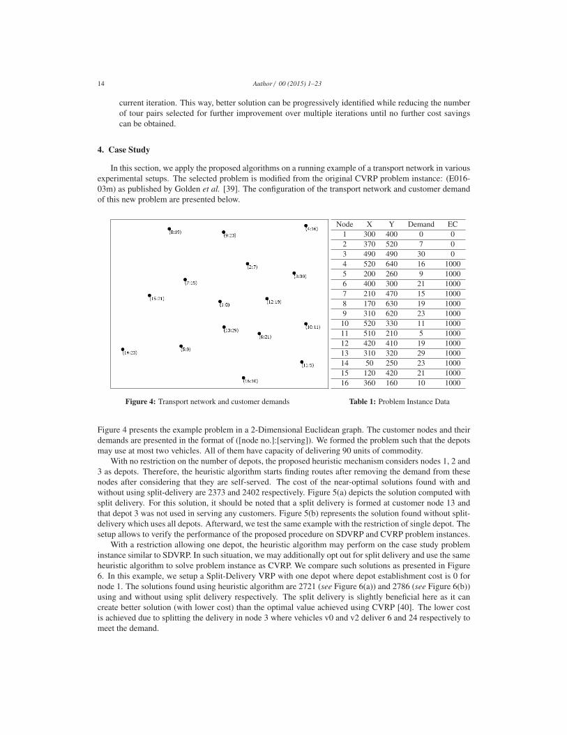
With no restriction on the number of depots, the proposed heuristic mechanism considers nodes 1, 2 and

3 as depots. Therefore, the heuristic algorithm starts finding routes after removing the demand from these

nodes after considering that they are self-served. The cost of the near-optimal solutions found with and

without using split-delivery are 2373 and 2402 respectively. Figure 5(a) depicts the solution computed with

split delivery. For this solution, it should be noted that a split delivery is formed at customer node 13 and

that depot 3 was not used in serving any customers. Figure 5(b) represents the solution found without split-

delivery which uses all depots. Afterward, we test the same example with the restriction of single depot. The

setup allows to verify the performance of the proposed procedure on SDVRP and CVRP problem instances.

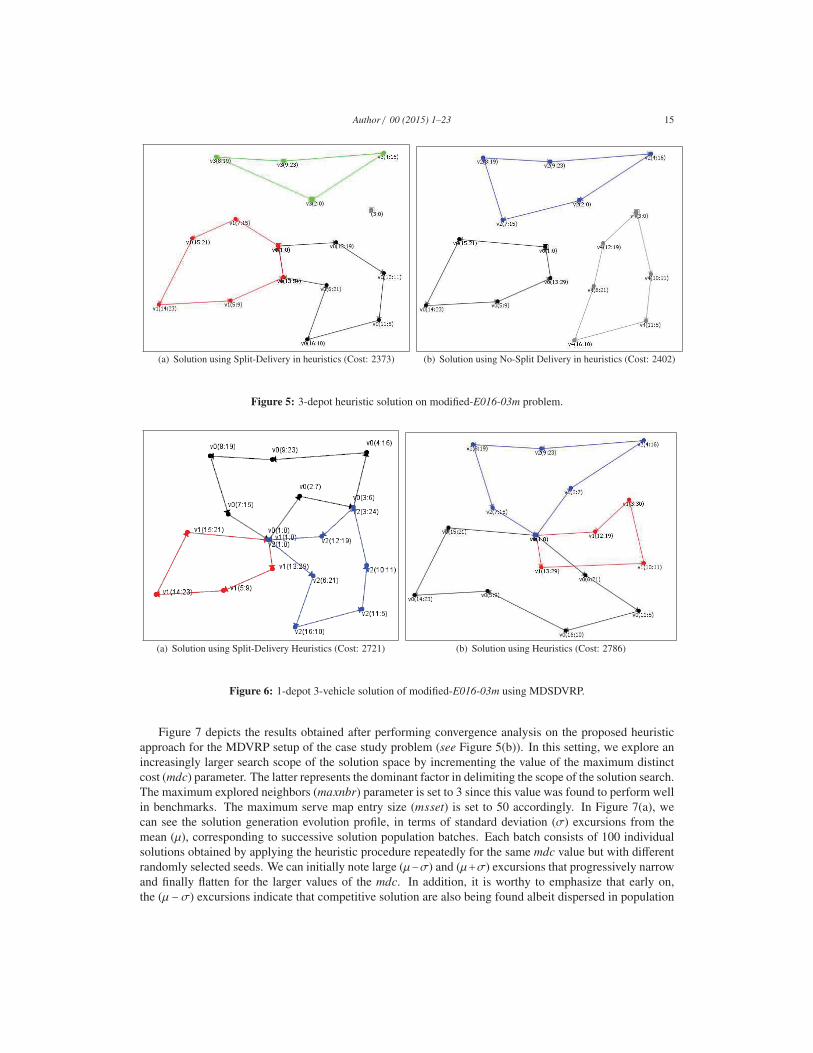
With a restriction allowing one depot, the heuristic algorithm may perform on the case study problem

instance similar to SDVRP. In such situation, we may additionally opt out for split delivery and use the same

heuristic algorithm to solve problem instance as CVRP. We compare such solutions as presented in Figure

6. In this example, we setup a Split-Delivery VRP with one depot where depot establishment cost is 0 for

node 1. The solutions found using heuristic algorithm are 2721 (see Figure 6(a)) and 2786 (see Figure 6(b))

using and without using split delivery respectively. The split delivery is slightly beneficial here as it can

create better solution (with lower cost) than the optimal value achieved using CVRP [40]. The lower cost

is achieved due to splitting the delivery in node 3 where vehicles v0 and v2 deliver 6 and 24 respectively to

meet the demand.

Author / 00 (2015) 1–23 15

(a) Solution using Split-Delivery in heuristics (Cost: 2373) (b) Solution using No-Split Delivery in heuristics (Cost: 2402)

Figure 5: 3-depot heuristic solution on modified-E016-03m problem.

(a) Solution using Split-Delivery Heuristics (Cost: 2721) (b) Solution using Heuristics (Cost: 2786)

Figure 6: 1-depot 3-vehicle solution of modified-E016-03m using MDSDVRP.

Figure 7 depicts the results obtained after performing convergence analysis on the proposed heuristic

approach for the MDVRP setup of the case study problem (see Figure 5(b)). In this setting, we explore an

increasingly larger search scope of the solution space by incrementing the value of the maximum distinct

cost (mdc) parameter. The latter represents the dominant factor in delimiting the scope of the solution search.

The maximum explored neighbors (maxnbr) parameter is set to 3 since this value was found to perform well

in benchmarks. The maximum serve map entry size (msset) is set to 50 accordingly. In Figure 7(a), we

can see the solution generation evolution profile, in terms of standard deviation (σ) excursions from the

mean (μ), corresponding to successive solution population batches. Each batch consists of 100 individual

solutions obtained by applying the heuristic procedure repeatedly for the same mdc value but with different

randomly selected seeds. We can initially note large (μ−σ) and (μ+σ) excursions that progressively narrow

and finally flatten for the larger values of the mdc. In addition, it is worthy to emphasize that early on,

the (μ −σ) excursions indicate that competitive solution are also being found albeit dispersed in population

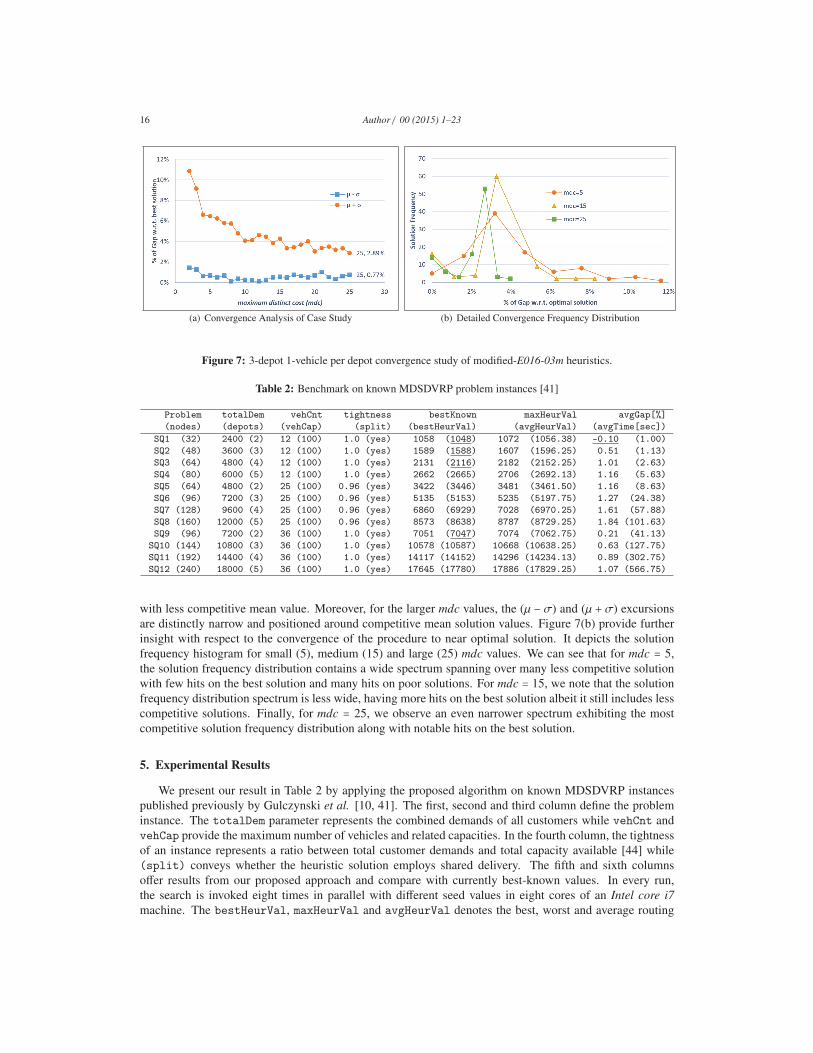
16 Author / 00 (2015) 1–23

(a) Convergence Analysis of Case Study (b) Detailed Convergence Frequency Distribution

Figure 7: 3-depot 1-vehicle per depot convergence study of modified-E016-03m heuristics.

Table 2: Benchmark on known MDSDVRP problem instances [41]

Problem totalDem vehCnt tightness bestKnown maxHeurVal avgGap[%]

(nodes) (depots) (vehCap) (split) (bestHeurVal) (avgHeurVal) (avgTime[sec])

SQ1 (32) 2400 (2) 12 (100) 1.0 (yes) 1058 (1048) 1072 (1056.38) -0.10 (1.00)

SQ2 (48) 3600 (3) 12 (100) 1.0 (yes) 1589 (1588) 1607 (1596.25) 0.51 (1.13)

SQ3 (64) 4800 (4) 12 (100) 1.0 (yes) 2131 (2116) 2182 (2152.25) 1.01 (2.63)

SQ4 (80) 6000 (5) 12 (100) 1.0 (yes) 2662 (2665) 2706 (2692.13) 1.16 (5.63)

SQ5 (64) 4800 (2) 25 (100) 0.96 (yes) 3422 (3446) 3481 (3461.50) 1.16 (8.63)

SQ6 (96) 7200 (3) 25 (100) 0.96 (yes) 5135 (5153) 5235 (5197.75) 1.27 (24.38)

SQ7 (128) 9600 (4) 25 (100) 0.96 (yes) 6860 (6929) 7028 (6970.25) 1.61 (57.88)

SQ8 (160) 12000 (5) 25 (100) 0.96 (yes) 8573 (8638) 8787 (8729.25) 1.84 (101.63)

SQ9 (96) 7200 (2) 36 (100) 1.0 (yes) 7051 (7047) 7074 (7062.75) 0.21 (41.13)

SQ10 (144) 10800 (3) 36 (100) 1.0 (yes) 10578 (10587) 10668 (10638.25) 0.63 (127.75)

SQ11 (192) 14400 (4) 36 (100) 1.0 (yes) 14117 (14152) 14296 (14234.13) 0.89 (302.75)

SQ12 (240) 18000 (5) 36 (100) 1.0 (yes) 17645 (17780) 17886 (17829.25) 1.07 (566.75)

with less competitive mean value. Moreover, for the larger mdc values, the (μ − σ) and (μ + σ) excursions

are distinctly narrow and positioned around competitive mean solution values. Figure 7(b) provide further

insight with respect to the convergence of the procedure to near optimal solution. It depicts the solution

frequency histogram for small (5), medium (15) and large (25) mdc values. We can see that for mdc = 5,

the solution frequency distribution contains a wide spectrum spanning over many less competitive solution

with few hits on the best solution and many hits on poor solutions. For mdc = 15, we note that the solution

frequency distribution spectrum is less wide, having more hits on the best solution albeit it still includes less

competitive solutions. Finally, for mdc = 25, we observe an even narrower spectrum exhibiting the most

competitive solution frequency distribution along with notable hits on the best solution.

5. Experimental Results

We present our result in Table 2 by applying the proposed algorithm on known MDSDVRP instances

published previously by Gulczynski et al. [10, 41]. The first, second and third column define the problem

instance. The totalDem parameter represents the combined demands of all customers while vehCnt and

vehCap provide the maximum number of vehicles and related capacities. In the fourth column, the tightness

of an instance represents a ratio between total customer demands and total capacity available [44] while

(split) conveys whether the heuristic solution employs shared delivery. The fifth and sixth columns

offer results from our proposed approach and compare with currently best-known values. In every run,

the search is invoked eight times in parallel with different seed values in eight cores of an Intel core i7machine. The bestHeurVal, maxHeurVal and avgHeurVal denotes the best, worst and average routing

Author / 00 (2015) 1–23 17

cost for a problem instance. The avgGap[%] in last column defines the percentage of the average gap of our

solution with respect to the best known value. avgTime[sec] is the average time taken to solve the problem

instance. The underlined values in column five and seven indicate finding of better result and average than

previously known solutions of the corresponding problem instances. The heuristic solutions are refined by

performing localized permutation on up to 4 adjacent nodes in a route. The routing details for the underlined

results are presented in the appendix. To solve the SQ problem series, the proposed algorithm uses mdc = 5,

msset = 100 and maxnbr = 1.

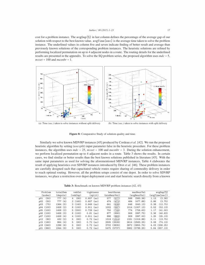
(a) Time (sec.) taken to solve instances without split delivery (b) Time (sec.) taken to solve instances with split delivery

Figure 8: Comparative Study of solution quality and time.

Similarly we solve known MDVRP instances [45] produced by Cordeau et al. [42]. We run the proposed

heuristic algorithm by setting (usesplit) input parameter false in the heuristic procedure. For these problem

instances, the algorithm uses mdc = 25, msset = 100 and maxnbr = 3. During the solution enhancement,

we perform localized permutation up to 4 adjacent nodes in a route. Table 3 shows the results. In certain

cases, we find similar or better results than the best known solutions published in literature [45]. With the

same input parameters as used for solving the aforementioned MDVRP instances, Table 4 elaborates the

result of applying heuristics over SDVRP instances introduced by Dror et al. [46]. These problem instances

are carefully designed such that capacitated vehicle routes require sharing of commodity delivery in order

to reach optimal routing. However, all the problem setups consist of one depot. In order to solve SDVRP

instances, we place a restriction over depot deployment cost and start heuristic search directly from a known

Table 3: Benchmark on known MDVRP problem instances [42, 43]

Problem totalDem vehCnt tightness bestKnown maxHeurVal avgGap[%]

(nodes) (depots) (vehCap) (split) (minHeurVal) (avgHeurVal) (avgTime[sec])

p01 (50) 777 (4) 4 (80) 0.607 (no) 577 (577) 588 (583.38) 1.13 (2.38)

p02 (50) 777 (4) 2 (160) 0.607 (no) 474 (472) 484 (477.88) 0.86 (3.75)

p03 (75) 1364 (5) 3 (140) 0.649 (no) 641 (638) 648 (643.13) 0.38 (12.75)

p04 (100) 1458 (2) 8 (100) 0.911 (no) 1002 (997) 1014 (1007.13) 0.52 (52.13)

p05 (100) 1458 (2) 5 (200) 0.729 (no) 750 (749) 774 (758.63) 1.17 (41.00)

p06 (100) 1458 (3) 6 (100) 0.81 (no) 877 (890) 906 (897.75) 2.36 (40.63)

p07 (100) 1458 (4) 4 (100) 0.911 (no) 886 (883) 909 (897.00) 1.25 (25.13)

p12 (80) 432 (2) 5 (60) 0.72 (no) 1319 (1314) 1331 (1319.88) 0.11 (13.75)

p15 (160) 864 (4) 5 (60) 0.72 (no) 2505 (2539) 2614 (2583.25) 3.08 (74.13)

p18 (240) 1296 (6) 5 (60) 0.72 (no) 3702 (3835) 3872 (3855.75) 4.03 (206.25)

p21 (360) 1944 (9) 5 (60) 0.72 (no) 5475 (5737) 5862 (5799.25) 5.64 (657.13)

18 Author / 00 (2015) 1–23

Table 4: Benchmark on known SDVRP problem instances [30]

Problem totalDem vehCnt tightness bestKnown maxHeurVal avgGap[%]

(nodes) (vehCap) (split) (minHeurVal) (avgHeurVal) (avgTime[sec])

eil22 (21) 22500 4(6000) 0.937 (no) 375 (375) 379 (378.00) 0.82 (1.00)

eil23 (22) 10189 3(4500) 0.754 (no) 569 (570) 570 (570.00) 0.20 (1.00)

eil30 (29) 12750 3(4500) 0.944 (yes) 510 (510) 511 (510.50) 0.10 (1.25)

eil33 (32) 29370 4(8000) 0.917 (no) 835 (841) 843 (842.33) 0.93 (3.00)

eil51 (50) 777 5 (160) 0.971 (no) 521 (521) 533 (525.67) 0.90 (13.67)

eilA76 (75) 1364 10 (140) 0.974 (yes) 832 (831) 841 (836.25) 0.55 (57.63)

eilA101 (100) 1458 8 (200) 0.911 (no) 817 (822) 831 (827.25) 1.29 (115.75)

eilB76 (75) 1364 14 (100) 0.974 (yes) 1023 (1010) 1032 (1024.63) 0.17 (34.38)

eilB101 (100) 1458 14 (112) 0.929 (yes) 1077 (1088) 1095 (1090.60) 1.28 (155.40)

eilC76 (75) 1364 8 (180) 0.947 (yes) 735 (741) 747 (745.00) 1.40 (47.00)

eilD76 (75) 1364 7 (220) 0.885 (no) 683 (691) 695 (692.63) 1.46 (49.38)

S51D1 (50) 402 3 (160) 0.837 (no) 458 (464) 481 (467.75) 2.13 (4.75)

S51D2 (50) 1415 9 (160) 0.982 (yes) 726 (707) 715 (711.00) -2.06 (5.00)

S51D3 (50) 2275 15 (160) 0.947 (yes) 972 (953) 970 (959.75) -1.22 (8.00)

S51D4 (50) 4317 27 (160) 0.999 (yes) 1677 (1561) 1581 (1569.75) -6.79 (75.00)

S51D5 (50) 3645 23 (160) 0.99 (yes) 1440 (1337) 1351 (1344.25) -7.09 (31.88)

S51D6 (50) 6459 41 (160) 0.984 (yes) 2327 (2182) 2196 (2187.25) -6.35 (418.63)

S76D1 (75) 614 4 (160) 0.959 (no) 594 (601) 628 (612.38) 3.04 (17.63)

S76D2 (75) 2383 15 (160) 0.992 (yes) 1147 (1091) 1108 (1099.25) -4.29 (36.37)

S76D3 (75) 3542 23 (160) 0.962 (yes) 1474 (1440) 1456 (1448.25) -1.74 (82.00)

S76D4 (75) 5765 37 (160) 0.973 (yes) 2257 (2096) 2115 (2102.25) -7.31 (547.25)

S101D1 (100) 788 5 (160) 0.985 (no) 716 (733) 748 (740.80) 3.40 (53.80)

S101D2 (100) 3064 20 (160) 0.957 (yes) 1393 (1383) 1403 (1395.00) 0.20 (82.63)

S101D3 (100) 4841 31 (160) 0.976 (yes) 1975 (1889) 1904 (1897.38) -4.05 (244.63)

S101D5 (100) 7679 48 (160) 0.999 (yes) 2915 (2814) 2866 (2828.63) -3.00 (874.63)

depot. With the presented input parameters, we achieve better results for many of these instances. Finally,

we also solve CVRP Augerat et. al [44] A, B and P problem set by restricting search from a given depot

and without using split. Table 5, Table 7 and Table 8 elaborate the results presented in the Appendix.

6. Results& Analysis

Figure 8 depicts an overall estimate of the time taken in solving all the problem instances considered in

Section 5. In both sub-figures, the solution time has been calculated for all the solved problem instances

with respect to number of customer nodes and vehicles. We depict the results by category based on the use

of split-delivery in solution. Figure 8 shows that the proposed technique is successful in solving CVRP,

SDVRP, MDVRP and MDSDVRP instances reasonably fast for small and medium scale problems. The so-

lution generation is faster especially in the cases where split-delivery is not used (see Figure 8(a)). However,

split-delivery (see Figure 8(b)) allows to generate good quality solutions which are some times better than

the best known values for these instances. After a careful analysis of the results, it becomes apparent that the

solving time increases notably with respect to customer nodes. On the other side, the increase in vehicles

also adversely affects the solution time.

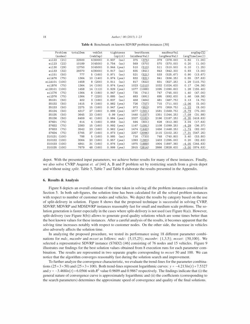
In analyzing the proposed procedure, we tested its performance using 18 different parameter combi-

nations for mdc, maxnbr and msset as follows: mdc: {5,15,25}; maxnbr: {1,3,5}; msset: {50,100}. We

selected a representative SDVRP instance (S76D2) [46] consisting of 76 nodes and 15 vehicles. Figure 9

illustrates our findings for the best solution values obtained from 8 execution runs for each parameter com-

bination. The results are represented in two separate graphs corresponding to msset 50 and 100. We can

notice that the algorithm converges reasonably fast during the solution search and improvement.

To further analyze the convergence characteristic, we evaluate the trend-lines for the parameter combina-

tions (25×3×50) and (25×3×100). Both trend-lines represent logarithmic curves: y = −4.213ln(t)+7.5327

and y = −3.468ln(t)+6.0566 with R2 value 0.9609 and 0.9867 respectively. The findings indicate that (i) the

general nature of convergence curve is approximately logarithmic and (ii) the coefficients (corresponding to

the search parameters) determines the approximate speed of convergence and quality of the final solutions.

Author / 00 (2015) 1–23 19

Figure 9: Convergence Study on SDVRP instance S76D2 [46] for multiple parameter values

In fact, faster convergence corresponds to diminished solution quality. Conversely, longer search time

leads to better solutions for appropriate parameter combinations. The lowest computation time is obtained

with parameter combinations (25×1×50) and (15×1×100) in the left and the right sub-figures respectively.

Likewise, the best solutions are obtained with parameter combinations (25 × 3 × 50) and (25 × 3 × 100) in

the left and the right sub-figures respectively. We may notice the level of dissimilarity with respect to the

solution finding trajectory when comparing the left (less similar) and right (more similar) sides of the figure.

Thus, we emphasize the selection of parameter combinations depending on the need in terms of time and

quality. We favored the combination (25 × 3 × 100) for conducting the bulk of our benchmark experiments.

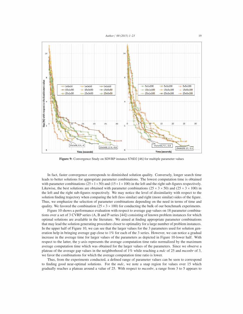
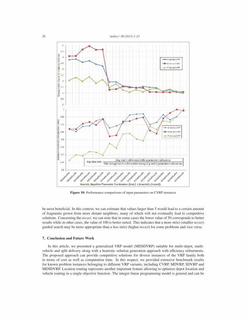
Figure 10 shows a performance evaluation with respect to average gap values on 18 parameter combina-

tions over a set of 3 CVRP series (A, B and P-series [44]) consisting of known problem instances for which

optimal solutions are available in the literature. We aimed at finding appropriate parameter combinations

that may lead the solution generating procedure closer to optimality for a large number of problem instances.

In the upper half of Figure 10, we can see that the larger values for the 3 parameters used for solution gen-

eration help in bringing average gap close to 1% for each of the 3 series. However, we can notice a gradual

increase in the average time for larger values of the parameters as depicted in Figure 10-lower half. With

respect to the latter, the y-axis represents the average computation time ratio normalized by the maximum

average computation time which was obtained for the larger values of the parameters. Since we observe a

plateau of the average gap values in the neighborhood of 1% while reaching a mdc of 25 and maxnbr of 3,

we favor the combinations for which the average computation time ratio is lower.

Thus, from the experiments conducted, a defined range of parameter values can be seen to correspond

to finding good near-optimal solutions. For the mdc, we note a snap region for values over 15 which

gradually reaches a plateau around a value of 25. With respect to maxnbr, a range from 3 to 5 appears to

20 Author / 00 (2015) 1–23

Figure 10: Performance comparisons of input parameters on CVRP instances

be most beneficial. In this context, we can estimate that values larger than 5 would lead to a certain amount

of fragments grown from more distant neighbors, many of which will not eventually lead to competitive

solutions. Concerning the msset, we can note that in some cases the lower value of 50 corresponds to better

results while in other cases, the value of 100 is better suited. This indicates that a more strict (smaller msset)guided search may be more appropriate than a less strict (higher msset) for some problems and vice versa.

7. Conclusion and Future Work

In this article, we presented a generalized VRP model (MDSDVRP) suitable for multi-depot, multi-

vehicle and split delivery along with a heuristic solution generation approach with efficiency refinements.

The proposed approach can provide competitive solutions for diverse instances of the VRP family both

in terms of cost as well as computation time. In this respect, we provided extensive benchmark results

for known problem instances belonging to different VRP variants, including CVRP, MDVRP, SDVRP and

MDSDVRP. Location routing represents another important feature allowing to optimize depot location and

vehicle routing in a single objective function. The integer linear programming model is general and can be

Author / 00 (2015) 1–23 21

customized to accommodate any of the aforementioned VRP family members. The accompanying solution

generation approach combines a generational stochastic cost insertion gradient descent technique with it-

erative solution improvement in order to produce competitive solutions. In addition, the heuristic solution

finding technique exhibits good scalability and performs well over various benchmark problem sets yielding

good near-optimal solutions. The use of split-delivery may help in better serving from a practical perspec-

tive and our results are especially notable in this context when compared to previous best known values. The

presented technique can be suitable for various transport management systems to quickly plan cost effec-

tive vehicle routes for product delivery. The proposed heuristic approach is flexible and allows for further

adaptation to accommodate other VRP settings.

The benchmark results show clear benefits in deriving routes using the proposed MDSDVRP solving

approach. In this respect, the discussed heuristics yields near optimal or even optimal values for many

instances. However, a trade-off exists between faster convergence and improved solution quality as deter-

mined by different values of the search parameters. It is important to emphasize that the node coordinates

are not needed in the search process and only the cost matrix is used. Consequently, the procedure is not

adversely affected by geometric considerations. The proposed technique is applicable in both Euclidean

non-Euclidean settings. This is an important aspect since in [25], it is shown that the solution approaches

based on the assumption of triangle inequality (e.g. Clarke-Wright Savings Algorithm) can be adversely

affected in terms of solution quality in case where this assumption does not hold. More specifically, the

solution quality increasingly degrades with the number of triangle inequality violations and in practice these

situations commonly arise in many real world vehicle routing scenarios. Our solution generation approach

is assessed up to hundreds of nodes and tens of vehicles. Also, it allows for parallelization (using different

randomizing seeds) and solution regeneration / re-tracing (when using the same randomizing seed). How-

ever, the proposed approach has some limitations in terms of single commodity delivery and the absence

of time-windows, which are the subject of future work. Other future work directions include extending

the technique to handle maximum vehicle tour cost and stochastic customer demands in centralized and

distributed setting.

References

[1] Z. Ozyurt, D. Aksen, Solving the multi-depot location-routing problem with lagrangian relaxation, in: Extending the Horizons:

Advances in Computing, Optimization, and Decision Technologies, Vol. 37 of Operations Research/Computer Science Interfaces

Series, Springer US, 2007, pp. 125–144.

[2] S. Salhi, G. K. Rand, The effect of ignoring routes when locating depots, European Journal of Operational Research 39 (2) (1989)

150–156.

[3] T. T. Schwartz, Y.-F. Pierre, E. Calpas, Building assessments and rubble removal in quake-affected neighborhoods in haiti, Barr

report, United States Agency for International Development (May 2011).

[4] Industry Canada, The list transportation, Canadian Investor Magazine 1 (3) (2012) 8–9.

[5] Staff Report, Bts says surface trade with nafta partners up 11.5 percent annually in january 2012, Logistics management, Bureau

of Transportation Statistics (March 2012).

[6] C. Eschinger, C. D. Klappich, Market trends: Transportation management systems worldwide; 2007-2012, Press Release

G00161482, Gartner Inc. (October 2008).

[7] E. M. Bartee, A holistic view of problem solving, Management Science 20 (4-part-i) (1973) 439–448.

[8] P. Toth, D. Vigo, An overview of vehicle routing problems, Society for Industrial and Applied Mathematics, Philadelphia, PA,

USA, 2002.

[9] C. Archetti, M. G. Speranza, Vehicle routing problems with split deliveries, International Transactions in Operational Research

19 (1-2) (2012) 3–22.

[10] D. Gulczynski, B. Golden, E. Wasil, The multi-depot split delivery vehicle routing problem: An integer programming-based

heuristic, new test problems, and computational results, Computers and Industrial Engineering 61 (3) (2011) 794 – 804.

[11] T. Feder, P. Hell, S. Klein, R. Motwani, Complexity of graph partition problems, in: Symposium on the Theory of Computing,

1999.

[12] K. Schloegel, G. Karypis, V. Kumar, Graph partitioning for high performance scientific simulations, Department of Computer

Science and Engineering, University of Minnesota (2000).

[13] S. Kucukpetek, F. Polat, H. Ogztuzun, Multilevel graph partitioning: An evolutionary approach, Journal of the Operational

Research Society (2005) 549–562.

[14] T. Oncan, S. N. Kabadi, K. Nair, Vlsn search algorithms for partitioning problems using matching neighborhoods, Journal of the

Operational Research Society (2008) 388–398.

[15] A. Jarrah, J. Bard, Pickup and delivery network segmentation using contiguous geographic clustering, Journal of the Operational

Research Society, advance online publication.

22 Author / 00 (2015) 1–23

[16] T. Kanungo, D. M. Mount, N. S. Netanyahu, C. D. Piatko, R. Silverman, A. Y. Wu, An efficient k-means clustering algorithm:

Analysis and implementation, IEEE Trans. Pattern Anal. Mach. Intell. 24 (7) (2002) 881–892.

[17] J. K. Antonio, G. M. Huang, W. K. Tsai, A fast distributed shortest path algorithm for a class of hierarchically clustered data

networks, IEEE Trans. Comput. 41 (6) (1992) 710–724.

[18] G. B. Dantzig, J. H. Ramser, The Truck Dispatching Problem, Management Science 6 (1) (1959) 80–91.

[19] B. Golden, S. Raghavan, E. A. Wasil, The vehicle routing problem: latest advances and new challenges, Operations re-

search/Computer science interfaces series, 43, Springer, 2008.

[20] M. Dror, P. Trudeau, Savings by split delivery routing, Transportation Science 23 (2) (1989) 141–145.

[21] C. Archetti, M. G. Speranza, An overview on the split delivery vehicle routing problem, in: K.-H. Waldmann, U. M. Stocker

(Eds.), Operations Research Proceedings 2006, Operations Research Proceedings, Springer Berlin Heidelberg, 2007, pp. 123–

127.

[22] C. Archetti, M. Speranza, The split delivery vehicle routing problem: A survey, in: B. Golden, S. Raghavan, E. Wasil (Eds.), The

Vehicle Routing Problem: Latest Advances and New Challenges, Vol. 43 of Operations Research/Computer Science Interfaces,

Springer US, 2008, pp. 103–122.

[23] S. Ray, A. Soeanu, M. Debbabi, A. Boukhtouta, J. Berger, Modeling multi-depot split-delivery vehicle routing problem, in: In

the Proceedings of the IEEE - Conference on Computational Engineering in Systems Applications, 2012.

[24] A. Soeanu, S. Ray, M. Debbabi, J. Berger, A. Boukhtouta, A learning based evolutionary algorithm for distributed multi-depot

vrp, in: KES, 2012, pp. 49–58.

[25] C. L. Fleming, S. E. Griffis, J. E. Bell, The effects of triangle inequality on the vehicle routing problem, European Journal of

Operational Research 224 (1) (2013) 1 – 7.

[26] M. Gronalt, R. Hartl, M. Reimann, New savings based algorithms for time constrained pickup and delivery of full truckloads,

European Journal of Operational Research (2008) 520–535.

[27] F. Chan, N. Kumar, Effective allocation of customers to distribution centres: A multiple ant colony optimization approach,

Robotics and Computer-Integrated Manufacturing (2009).

[28] G. Zhou, H. Min, M. Gen, The balanced allocation of customers to multiple distribution centers in the supply chain network: a

genetic algorithm approach, in: Computers and Industrial Engineering, 2002, pp. 251–261.

[29] S. Arunapuram, K. Mathur, D. Solow, Vehicle routing and scheduling with full truckloads, in: Transportation Science, 2003, pp.

170–182.

[30] M. Dror, G. Laporte, P. Trudeau, Vehicle routing with split deliveries, Discrete Applied Mathematics 50 (3) (1994) 239 – 254.

[31] L. Ozdamar, E. Ekinci, B. Kucukyazici, Emergency logistics planning in natural disasters, Annals of Operations Research (2004)

217–245.

[32] W. Yi, A. Kumar, Ant colony optimization for disaster relief operations, in: Transportation Research Part E: Logistics and

Transportation Review, 2007, pp. 660–672.

[33] A. Soeanu, S. Ray, M. Debbabi, J. Berger, A. Boukhtouta, A. Ghanmi, A decentralized heuristic for multi-depot split-delivery

vehicle routing problem, in: IEEE-ICAL, 2011.

[34] B. Yu, Z. Z. Yang, J.-X. Xie, A parallel improved ant colony optimization for multi-depot vehicle routing problem., JORS 62 (1)

(2011) 183–188.

[35] P. Toth, D. Vigo, The Vehicle Routing Problem, Society for Industrial and Applied Mathematics, 2002.

[36] S. Dash, Mixed integer rounding cuts and master group polyhedra, in: Combinatorial Optimization - Methods and Applications,

2011, pp. 1–32.

[37] H. Abeledo, M. Bussieck, L. Lasdon, A. Meeraus, H. Ni, Global optimization and the gams branch-and cut facility,

CORS/INFORMS Joint International Workshop, Banff (May 2004).

[38] N. Kokash, An introduction to heuristic algorithms.

[39] B. L. Golden, E. A. Wasil, J. P. Kelly, I.-M. Chao, Metaheuristics in vehicle routing, Kluwer, Boston, 1998, Ch. Fleet Management

and Logistics.

[40] M. Iori, J.-J. Salazar-González, D. Vigo, An exact approach for the vehicle routing problem with two-dimensional loading

constraints, Transportation Science 41 (2) (2007) 253–264.

[41] D. J. Gulczynski, Integer programming-based heuristics for vehicle routing problems, Ph.D. thesis, Robert H. Smith School of

Business, University of Maryland, USA (2010).

[42] J.-F. Cordeau, M. Gendreau, G. Laporte, A tabu search heuristic for periodic and multi-depot vehicle routing problems, Networks

30 (2) (1997) 105–119.

[43] B. Crevier, J.-F. Cordeau, G. Laporte, The multi-depot vehicle routing problem with inter-depot routes, European Journal of

Operational Research 176 (2) (2007) 756–773.

[44] P. Augerat, J. Belenguer, E. Benavent, A. Corberan, D. Naddef, G. Rinaldi, Computational results with a branch and cut code for

the capacitated vehicle routing problem, Tech. rep., Universite Joseph Fourier, Grenoble, France (1995).

[45] E.T.S. Ingenieria Informatica of the University of Malaga, Networking and emerging optimization, online; http://neo.lcc.

uma.es/vrp/.

[46] S. Chen, B. L. Golden, E. A. Wasil, The split delivery vehicle routing problem: Applications, algorithms, test problems, and

computational results, Networks 49 (4) (2007) 318–329.

Author / 00 (2015) 1–23 23

Appendix

Table 5: Benchmark on known CVRP problem instances: A-Set from Augerat et al.[44]- Part 1

Problem totalDem vehCnt tightness bestKnown maxHeurVal avgGap[%]

(nodes) (depots) (vehCap) (split) (minHeurVal) (avgHeurVal) (avgTime[sec])

A-n32-k5 (31) 410 (1) 5 (100) 0.82 (no) 784 (784) 791 (785.31) 0.17 (2.31)

A-n33-k5 (32) 446 (1) 5 (100) 0.892 (no) 661 (661) 669 (663.25) 0.34 (1.50)

A-n33-k6 (32) 541 (1) 6 (100) 0.901 (no) 742 (742) 745 (742.31) 0.06 (1.38)

A-n34-k5 (33) 460 (1) 5 (100) 0.92 (no) 778 (778) 791 (784.92) 0.92 (1.42)

A-n34-k5 (33) 460 (1) 5 (100) 0.92 (yes) 778 (780) 783 (782.25) 0.60 (2.25)

A-n36-k5 (35) 442 (1) 5 (100) 0.884 (no) 799 (799) 829 (818.53) 2.41 (4.13)

A-n36-k5 (35) 442 (1) 5 (100) 0.884 (yes) 799 (820) 820 (820.00) 2.60 (3.00)

A-n37-k5 (36) 407 (1) 5 (100) 0.814 (no) 669 (670) 691 (680.19) 1.68 (5.19)

A-n37-k6 (36) 570 (1) 6 (100) 0.95 (no) 949 (955) 972 (965.00) 1.70 (2.75)

A-n37-k6 (36) 570 (1) 6 (100) 0.95 (yes) 949 (948) 968 (958.00) 0.99 (5.00)

A-n38-k5 (37) 481 (1) 5 (100) 0.962 (no) 730 (730) 739 (731.80) 0.28 (3.40)

A-n38-k5 (37) 481 (1) 5 (100) 0.962 (yes) 730 (724) 745 (730.17) 0.08 (4.50)

A-n39-k5 (38) 475 (1) 5 (100) 0.95 (no) 822 (822) 830 (826.56) 0.58 (3.89)

A-n39-k5 (38) 475 (1) 5 (100) 0.95 (yes) 822 (825) 840 (829.71) 0.99 (4.86)

A-n39-k6 (38) 526 (1) 6 (100) 0.876 (no) 831 (833) 841 (834.79) 0.50 (5.50)

A-n39-k6 (38) 526 (1) 6 (100) 0.876 (yes) 831 (834) 834 (834.00) 0.40 (4.00)

A-n44-k6 (43) 570 (1) 6 (100) 0.95 (no) 937 (937) 955 (943.69) 0.73 (7.08)

A-n44-k6 (43) 570 (1) 6 (100) 0.95 (yes) 937 (937) 938 (937.33) 0.07 (4.33)

A-n45-k6 (44) 593 (1) 6 (100) 0.988 (no) 944 (948) 966 (952.88) 0.99 (6.63)

A-n45-k6 (44) 593 (1) 6 (100) 0.988 (yes) 944 (932) 943 (938.63) -0.54 (9.13)

A-n45-k7 (44) 634 (1) 7 (100) 0.905 (no) 1146 (1151) 1164 (1157.91) 1.07 (6.82)

A-n45-k7 (44) 634 (1) 7 (100) 0.905 (yes) 1146 (1154) 1171 (1159.80) 1.24 (11.40)

A-n46-k7 (45) 603 (1) 7 (100) 0.861 (no) 914 (915) 948 (920.36) 0.75 (9.00)

A-n46-k7 (45) 603 (1) 7 (100) 0.861 (yes) 914 (926) 935 (929.00) 1.66 (10.20)

A-n48-k7 (47) 626 (1) 7 (100) 0.894 (no) 1073 (1073) 1112 (1101.62) 2.64 (13.08)

A-n48-k7 (47) 626 (1) 7 (100) 0.894 (yes) 1073 (1078) 1085 (1082.67) 0.97 (12.00)

A-n53-k7 (52) 664 (1) 7 (100) 0.948 (no) 1010 (1014) 1036 (1025.25) 1.52 (13.88)

A-n53-k7 (52) 664 (1) 7 (100) 0.948 (yes) 1010 (1008) 1023 (1015.75) 0.60 (16.50)

A-n54-k7 (53) 669 (1) 7 (100) 0.955 (no) 1167 (1173) 1190 (1180.13) 1.19 (16.88)

A-n54-k7 (53) 669 (1) 7 (100) 0.955 (yes) 1167 (1171) 1179 (1174.50) 0.69 (29.38)

A-n55-k9 (54) 839 (1) 9 (100) 0.932 (no) 1073 (1074) 1103 (1082.78) 0.93 (10.00)

A-n55-k9 (54) 839 (1) 9 (100) 0.932 (yes) 1073 (1074) 1093 (1082.00) 0.86 (16.71)

A-n60-k9 (59) 829 (1) 9 (100) 0.921 (no) 1354 (1357) 1377 (1364.45) 0.83 (27.18)

A-n60-k9 (59) 829 (1) 9 (100) 0.921 (yes) 1354 (1357) 1375 (1363.20) 0.72 (38.00)

A-n61-k9 (60) 885 (1) 9 (100) 0.983 (no) 1035 (1038) 1052 (1043.38) 0.84 (19.13)

A-n61-k9 (60) 885 (1) 9 (100) 0.983 (yes) 1034 (1022) 1028 (1025.63) -0.74 (36.63)

A-n62-k8 (61) 733 (1) 8 (100) 0.916 (no) 1290 (1310) 1325 (1319.46) 2.28 (37.69)

A-n62-k8 (61) 733 (1) 8 (100) 0.916 (yes) 1290 (1314) 1321 (1316.67) 2.10 (42.33)

A-n63-k9 (62) 873 (1) 9 (100) 0.97 (no) 1616 (1630) 1648 (1633.13) 1.10 (26.13)

A-n63-k9 (62) 873 (1) 9 (100) 0.97 (yes) 1616 (1625) 1633 (1627.50) 0.76 (36.13)

A-n63-k10 (62) 932 (1) 10 (100) 0.932 (no) 1315 (1321) 1330 (1325.50) 0.86 (23.63)

A-n63-k10 (62) 932 (1) 10 (100) 0.932 (yes) 1315 (1312) 1329 (1321.50) 0.54 (38.25)

A-n64-k9 (63) 848 (1) 9 (100) 0.942 (no) 1402 (1427) 1450 (1437.13) 2.51 (29.63)

A-n64-k9 (63) 848 (1) 9 (100) 0.942 (yes) 1402 (1410) 1443 (1429.00) 1.95 (42.25)

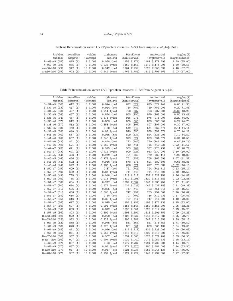
24 Author / 00 (2015) 1–23

Table 6: Benchmark on known CVRP problem instances: A-Set from Augerat et al.[44]- Part 2

Problem totalDem vehCnt tightness bestKnown maxHeurVal avgGap[%]

(nodes) (depots) (vehCap) (split) (minHeurVal) (avgHeurVal) (avgTime[sec])

A-n69-k9 (68) 845 (1) 9 (100) 0.938 (no) 1159 (1171) 1181 (1174.89) 1.39 (35.00)

A-n69-k9 (68) 845 (1) 9 (100) 0.938 (yes) 1159 (1168) 1179 (1174.00) 1.30 (38.57)

A-n80-k10 (79) 942 (1) 10 (100) 0.942 (no) 1764 (1799) 1823 (1806.33) 2.40 (67.78)

A-n80-k10 (79) 942 (1) 10 (100) 0.942 (yes) 1764 (1785) 1816 (1799.86) 2.03 (97.00)

Table 7: Benchmark on known CVRP problem instances: B-Set from Augerat et al.[44]

Problem totalDem vehCnt tightness bestKnown maxHeurVal avgGap[%]

(nodes) (depots) (vehCap) (split) (minHeurVal) (avgHeurVal) (avgTime[sec])

B-n31-k5 (30) 412 (1) 5 (100) 0.824 (no) 672 (672) 675 (672.44) 0.08 (1.38)

B-n34-k5 (33) 457 (1) 5 (100) 0.914 (no) 788 (789) 789 (789.00) 0.20 (1.88)

B-n34-k5 (33) 457 (1) 5 (100) 0.914 (yes) 788 (782) 783 (782.50) -0.65 (3.25)

B-n35-k5 (34) 437 (1) 5 (100) 0.874 (no) 955 (956) 979 (962.60) 0.86 (3.47)

B-n35-k5 (34) 437 (1) 5 (100) 0.874 (yes) 955 (976) 976 (976.00) 2.20 (4.00)

B-n38-k6 (37) 512 (1) 6 (100) 0.853 (no) 805 (805) 809 (806.80) 0.27 (4.73)

B-n38-k6 (37) 512 (1) 6 (100) 0.853 (yes) 805 (807) 807 (807.00) 0.30 (7.00)

B-n39-k5 (38) 440 (1) 5 (100) 0.88 (no) 549 (549) 571 (560.67) 2.11 (4.11)

B-n39-k5 (38) 440 (1) 5 (100) 0.88 (yes) 549 (550) 555 (552.57) 0.70 (4.29)

B-n41-k6 (40) 567 (1) 6 (100) 0.945 (no) 829 (834) 844 (838.20) 1.12 (4.50)

B-n41-k6 (40) 567 (1) 6 (100) 0.945 (yes) 829 (827) 839 (831.67) 0.37 (8.50)

B-n43-k6 (42) 521 (1) 6 (100) 0.868 (no) 742 (742) 749 (744.69) 0.42 (9.77)

B-n43-k6 (42) 521 (1) 6 (100) 0.868 (yes) 742 (741) 746 (743.33) 0.23 (11.67)

B-n44-k7 (43) 641 (1) 7 (100) 0.915 (no) 909 (909) 932 (925.79) 1.86 (8.71)

B-n44-k7 (43) 641 (1) 7 (100) 0.915 (yes) 909 (927) 933 (930.00) 2.30 (10.00)

B-n45-k5 (44) 486 (1) 5 (100) 0.972 (no) 751 (760) 772 (765.11) 1.90 (8.89)

B-n45-k5 (44) 486 (1) 5 (100) 0.972 (yes) 751 (758) 768 (763.29) 1.67 (11.57)

B-n45-k6 (44) 592 (1) 6 (100) 0.986 (no) 678 (678) 691 (682.50) 0.68 (8.88)

B-n45-k6 (44) 592 (1) 6 (100) 0.986 (yes) 678 (674) 677 (675.38) -0.32 (10.13)

B-n50-k7 (49) 609 (1) 7 (100) 0.87 (no) 741 (741) 744 (741.71) 0.13 (15.14)

B-n50-k7 (49) 609 (1) 7 (100) 0.87 (yes) 741 (743) 744 (743.50) 0.40 (19.50)

B-n50-k8 (49) 735 (1) 8 (100) 0.918 (no) 1312 (1319) 1332 (1327.75) 1.26 (14.88)

B-n50-k8 (49) 735 (1) 8 (100) 0.918 (yes) 1312 (1293) 1330 (1314.38) 0.22 (23.88)

B-n51-k7 (50) 684 (1) 7 (100) 0.977 (no) 1032 (1032) 1047 (1036.75) 0.47 (11.00)

B-n51-k7 (50) 684 (1) 7 (100) 0.977 (yes) 1032 (1026) 1042 (1034.75) 0.31 (19.38)

B-n52-k7 (51) 606 (1) 7 (100) 0.865 (no) 747 (748) 753 (751.54) 0.62 (15.69)

B-n52-k7 (51) 606 (1) 7 (100) 0.865 (yes) 747 (751) 753 (752.00) 0.70 (16.67)

B-n56-k7 (55) 616 (1) 7 (100) 0.88 (no) 707 (709) 716 (712.93) 0.87 (25.87)

B-n56-k7 (55) 616 (1) 7 (100) 0.88 (yes) 707 (717) 717 (717.00) 1.40 (20.00)

B-n57-k7 (56) 697 (1) 7 (100) 0.995 (no) 1153 (1158) 1192 (1173.13) 1.75 (22.00)

B-n57-k7 (56) 697 (1) 7 (100) 0.995 (yes) 1153 (1147) 1159 (1153.00) 0.05 (32.38)

B-n57-k9 (56) 803 (1) 9 (100) 0.892 (no) 1598 (1601) 1628 (1612.25) 0.93 (15.25)

B-n57-k9 (56) 803 (1) 9 (100) 0.892 (yes) 1598 (1594) 1613 (1601.75) 0.29 (28.25)

B-n63-k10 (62) 922 (1) 10 (100) 0.922 (no) 1496 (1537) 1548 (1542.38) 3.05 (29.75)

B-n63-k10 (62) 922 (1) 10 (100) 0.922 (yes) 1496 (1484) 1547 (1515.25) 1.29 (38.13)

B-n64-k9 (63) 878 (1) 9 (100) 0.975 (no) 861 (867) 881 (875.75) 1.71 (30.50)

B-n64-k9 (63) 878 (1) 9 (100) 0.975 (yes) 861 (861) 869 (865.13) 0.54 (49.00)

B-n66-k9 (65) 861 (1) 9 (100) 0.956 (no) 1316 (1318) 1332 (1323.00) 0.60 (36.63)

B-n66-k9 (65) 861 (1) 9 (100) 0.956 (yes) 1316 (1315) 1322 (1318.38) 0.24 (46.88)

B-n67-k10 (66) 907 (1) 10 (100) 0.907 (no) 1032 (1065) 1078 (1072.70) 3.83 (36.90)

B-n67-k10 (66) 907 (1) 10 (100) 0.907 (yes) 1032 (1040) 1075 (1059.33) 2.58 (53.17)

B-n68-k9 (67) 837 (1) 9 (100) 0.93 (no) 1272 (1287) 1294 (1289.88) 1.44 (40.75)

B-n68-k9 (67) 837 (1) 9 (100) 0.93 (yes) 1272 (1270) 1290 (1281.00) 0.74 (52.50)

B-n78-k10 (77) 937 (1) 10 (100) 0.937 (no) 1221 (1237) 1254 (1244.13) 1.91 (76.00)

B-n78-k10 (77) 937 (1) 10 (100) 0.937 (yes) 1221 (1222) 1247 (1232.50) 0.97 (97.38)

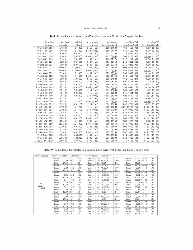
Author / 00 (2015) 1–23 25

Table 8: Benchmark on known CVRP problem instances: P-Set from Augerat et al.[44]

Problem totalDem vehCnt tightness bestKnown maxHeurVal avgGap[%]

(nodes) (depots) (vehCap) (split) (minHeurVal) (avgHeurVal) (avgTime[sec])

P-n16-k8 (15) 246 (1) 8 (35) 1.13 (no) 450 (450) 450 (450.00) 0.00 (1.00)

P-n16-k8 (15) 246 (1) 8 (35) 1.13 (yes) 450 (440) 440 (440.00) -2.20 (1.00)

P-n19-k2 (18) 310 (1) 2 (160) 1.03 (no) 212 (212) 212 (212.00) 0.00 (1.00)

P-n19-k2 (18) 310 (1) 2 (160) 1.03 (yes) 212 (205) 205 (205.00) -3.40 (1.00)

P-n20-k2 (19) 310 (1) 2 (160) 1.03 (no) 216 (217) 217 (217.00) 0.50 (1.00)

P-n21-k2 (20) 298 (1) 2 (160) 1.07 (no) 211 (211) 211 (211.00) 0.00 (1.00)

P-n22-k2 (21) 308 (1) 2 (160) 1.03 (no) 216 (216) 216 (216.00) 0.00 (1.00)

P-n22-k8 (21) 22500 (1) 8 (3000) 1.06 (no) 603 (603) 603 (603.00) 0.00 (1.00)

P-n22-k8 (21) 22500 (1) 8 (3000) 1.06 (yes) 603 (575) 586 (577.38) -4.38 (1.00)

P-n23-k8 (22) 313 (1) 8 (40) 1.02 (no) 529 (529) 533 (529.50) 0.10 (1.00)

P-n23-k8 (22) 313 (1) 8 (40) 1.02 (yes) 529 (511) 519 (512.75) -3.15 (1.00)

P-n40-k5 (39) 618 (1) 5 (140) 1.13 (no) 458 (458) 464 (459.27) 0.29 (4.87)

P-n45-k5 (44) 692 (1) 5 (150) 1.08 (no) 510 (510) 520 (516.08) 1.22 (5.92)

P-n50-k10 (49) 951 (1) 10 (100) 1.05 (no) 696 (697) 707 (702.25) 0.92 (2.63)

P-n50-k10 (49) 951 (1) 10 (100) 1.05 (yes) 696 (692) 699 (696.25) 0.08 (4.50)

P-n50-k7 (49) 951 (1) 7 (150) 1.1 (no) 554 (556) 565 (560.07) 1.12 (8.47)

P-n50-k8 (49) 951 (1) 8 (120) 1.0 (no) 631 (638) 645 (641.38) 1.65 (4.50)

P-n50-k8 (49) 951 (1) 8 (120) 1.0 (yes) 631 (618) 622 (619.50) -1.82 (10.38)

P-n51-k10 (50) 777 (1) 10 (80) 1.02 (no) 741 (741) 756 (747.25) 0.86 (3.50)

P-n51-k10 (50) 777 (1) 10 (80) 1.02 (yes) 741 (730) 739 (733.88) -0.94 (4.50)

P-n55-k10 (54) 1042 (1) 10 (115) 1.1 (no) 694 (696) 702 (700.00) 0.89 (5.36)

P-n55-k15 (54) 1042 (1) 15 (70) 1.0 (no) 989 (996) 1067 (1024.75) 3.49 (14.00)

P-n55-k15 (54) 1042 (1) 15 (70) 1.0 (yes) 989 (922) 937 (928.00) -6.52 (11.38)

P-n55-k7 (54) 1042 (1) 7 (170) 1.14 (no) 568 (575) 579 (576.20) 1.48 (16.07)

P-n60-k10 (59) 1134 (1) 10 (120) 1.05 (no) 744 (750) 756 (752.50) 1.16 (8.50)

P-n60-k10 (59) 1134 (1) 10 (120) 1.05 (yes) 744 (742) 755 (749.25) 0.74 (17.50)

P-n60-k15 (59) 1134 (1) 15 (80) 1.05 (no) 968 (975) 980 (976.25) 0.93 (9.50)

P-n60-k15 (59) 1134 (1) 15 (80) 1.05 (yes) 968 (965) 971 (968.25) 0.09 (10.38)

P-n65-k10 (64) 1219 (1) 10 (130) 1.06 (no) 792 (800) 806 (802.33) 1.32 (19.08)

P-n70-k10 (69) 1313 (1) 10 (135) 1.02 (no) 827 (835) 845 (837.25) 1.26 (28.13)

P-n70-k10 (69) 1313 (1) 10 (135) 1.02 (yes) 827 (825) 837 (830.25) 0.41 (43.25)

P-n76-k4 (75) 1364 (1) 4 (350) 1.02 (no) 593 (598) 614 (606.31) 2.24 (19.23)

P-n76-k5 (75) 1364 (1) 5 (280) 1.02 (no) 627 (630) 648 (638.43) 1.83 (22.07)

P-n101-k4 (100) 1458 (1) 4 (400) 1.09 (no) 681 (696) 735 (718.31) 5.23 (40.75)

Table 9: Route details for selected solutions from SQ-Series with better than the best known cost.

Problem[sol] Solution Details (segments): tour serve / tour cost

SQ1

(split)

[1048]

Route 0, 1, 2,0 (3)

Serve 0,80,20,0 100

Cost 14,10,10 34

Route 0, 8, 7,0 (3)

Serve 0,85,15,0 100

Cost 14,10,10 34

Route 0, 3, 5,0 (3)

Serve 0,80,20,0 100

Cost 14,10,10 34

Route 0, 4, 6,0 (3)

Serve 0,20,80,0 100

Cost 10,10,14 34

Route 0, 2,10,0 (3)

Serve 0,40,60,0 100

Cost 10,10,20 40

Route 0, 4,12,0 (3)

Serve 0,40,60,0 100

Cost 10,10,20 40

Route 0, 5,13,0 (3)

Serve 0,40,60,0 100

Cost 10,10,20 40

Route 0,15, 7,0 (3)

Serve 0,55,45,0 100

Cost 20,10,10 40

Route 0,11, 3,0 (3)

Serve 0,90,10,0 100

Cost 28,14,14 56

Route 0, 9, 1,0 (3)

Serve 0,90,10,0 100

Cost 28,14,14 56

Route 0, 8,16,27,0 (4)

Serve 0, 5,85,10,0 100

Cost 14,14, 2,30 60

Route 0, 6,14,25,0 (4)

Serve 0,10,85, 5,0 100

Cost 14,14, 2,30 60

Route 33,19,18,33 (3)

Serve 0,75,25, 0 100

Cost 14,10,10 34

Route 33,17,20,33 (3)

Serve 0,80,20, 0 100

Cost 14,10,10 34

Route 33,21,24,33 (3)

Serve 0,20,80, 0 100

Cost 10,10,14 34

Route 33,23,22,33 (3)

Serve 0,20,80, 0 100

Cost 10,10,14 34

Route 33,31,23,33 (3)

Serve 0,60,40, 0 100

Cost 20,10,10 40

Route 33,28,20,33 (3)

Serve 0,60,40, 0 100

Cost 20,10,10 40

Route 33,18,26,33 (3)

Serve 0,35,65, 0 100

Cost 10,10,20 40

Route 33,29,21,33 (3)

Serve 0,60,40, 0 100

Cost 20,10,10 40

Route 33,25,17,33 (3)

Serve 0,90,10, 0 100

Cost 28,14,14 56

Route 33,32,24,33 (3)

Serve 0,90,10, 0 100

Cost 28,14,14 56

Route 33,19,27,33 (3)

Serve 0,15,85, 0 100

Cost 14,14,28 56

Route 33,22,30,33 (3)

Serve 0,10,90, 0 100

Cost 14,14,28 56

26 Author / 00 (2015) 1–23

Pb.[sol] Solution Details (segments): tour serve / tour cost

SQ2

(split)

[1588]

Route 0, 8, 7,0 (3)

Serve 0,90,10,0 100

Cost 14,10,10 34

Route 0, 2, 1,0 (3)

Serve 0,20,80,0 100

Cost 10,10,14 34

Route 0, 4, 6,0 (3)

Serve 0,20,80,0 100

Cost 10,10,14 34

Route 0, 3, 5,0 (3)

Serve 0,80,20,0 100

Cost 14,10,10 34

Route 0,10, 2,0 (3)

Serve 0,60,40,0 100

Cost 20,10,10 40

Route 0, 4,12,0 (3)

Serve 0,40,60,0 100

Cost 10,10,20 40

Route 0,13, 5,0 (3)

Serve 0,60,40,0 100

Cost 20,10,10 40

Route 0,15, 7,0 (3)

Serve 0,50,50,0 100

Cost 20,10,10 40

Route 0,11, 3,0 (3)

Serve 0,90,10,0 100

Cost 28,14,14 56

Route 0, 1, 9,0 (3)

Serve 0,10,90,0 100

Cost 14,14,28 56

Route 0,14,25, 6,0 (4)

Serve 0,85, 5,10,0 100

Cost 28, 2,16,14 60

Route 0,16,27,0 (3)

Serve 0,85,15,0 100

Cost 28, 2,30 60

Route 49,20,17,49 (3)

Serve 0,20,80, 0 100

Cost 10,10,14 34

Route 49,18,19,49 (3)

Serve 0,60,40, 0 100

Cost 10,10,14 34

Route 49,21,24,49 (3)

Serve 0,30,70, 0 100

Cost 10,10,14 34

Route 49,23,22,49 (3)

Serve 0,20,80, 0 100

Cost 10,10,14 34

Route 49,28,20,49 (3)

Serve 0,60,40, 0 100

Cost 20,10,10 40

Route 49,31,23,49 (3)

Serve 0,60,40, 0 100

Cost 20,10,10 40

Route 49,29,44,21,49 (4)

Serve 0,65, 5,30, 0 100

Cost 20, 2,12,10 44

Route 49,19,26,15,49 (4)

Serve 0,30,65, 5, 0 100

Cost 14,14, 2,22 52

Route 49,17,25,49 (3)

Serve 0,10,90, 0 100

Cost 14,14,28 56

Route 49,24,32,49 (3)

Serve 0,20,80, 0 100

Cost 14,14,28 56

Route 49,22,30,49 (3)

Serve 0,10,90, 0 100

Cost 14,14,28 56

Route 49,19,27,49 (3)

Serve 0,20,80, 0 100

Cost 14,14,28 56

Route 50,38,36,50 (3)

Serve 0,90,10, 0 100

Cost 14,10,10 34

Route 50,33,34,50 (3)

Serve 0,80,20, 0 100

Cost 14,10,10 34

Route 50,37,35,50 (3)

Serve 0,20,80, 0 100

Cost 10,10,14 34

Route 50,40,39,50 (3)

Serve 0,80,20, 0 100

Cost 14,10,10 34

Route 50,44,36,50 (3)

Serve 0,50,50, 0 100

Cost 20,10,10 40

Route 50,34,42,50 (3)

Serve 0,40,60, 0 100

Cost 10,10,20 40

Route 50,39,47,50 (3)

Serve 0,40,60, 0 100

Cost 10,10,20 40

Route 50,37,45,50 (3)

Serve 0,40,60, 0 100

Cost 10,10,20 40

Route 50,35,43,50 (3)

Serve 0,10,90, 0 100

Cost 14,14,28 56

Route 50,33,41,50 (3)

Serve 0,10,90, 0 100

Cost 14,14,28 56

Route 50,40,48,50 (3)

Serve 0,10,90, 0 100

Cost 14,14,28 56

Route 50,46,32,50 (3)

Serve 0,85,15, 0 100

Cost 28, 2,30 60

SQ3

(split)

[2116]

Route 0, 5, 3,0 (3)

Serve 0,15,85,0 100

Cost 10,10,14 34

Route 0, 7, 8,0 (3)

Serve 0,25,75,0 100

Cost 10,10,14 34

Route 0, 2, 1,0 (3)

Serve 0,20,80,0 100

Cost 10,10,14 34

Route 0, 4, 6,0 (3)

Serve 0,20,80,0 100

Cost 10,10,14 34

Route 0,13, 5,0 (3)

Serve 0,55,45,0 100

Cost 20,10,10 40

Route 0, 2,10,0 (3)

Serve 0,40,60,0 100

Cost 10,10,20 40

Route 0, 4,12,0 (3)

Serve 0,40,60,0 100

Cost 10,10,20 40

Route 0,26,15, 7,0 (4)

Serve 0,10,55,35,0 100

Cost 22, 2,10,10 44

Route 0, 9, 1,0 (3)

Serve 0,90,10,0 100

Cost 28,14,14 56

Route 0, 8,16,0 (3)

Serve 0,15,85,0 100

Cost 14,14,28 56

Route 0, 3,11,57,0 (4)

Serve 0, 5,85,10,0 100

Cost 14,14, 2,30 60

Route 0,14,25, 6,0 (4)

Serve 0,85, 5,10,0 100

Cost 28, 2,16,14 60

Route 65,24,21,65 (3)

Serve 0,70,30, 0 100

Cost 14,10,10 34

Route 65,20,17,65 (3)

Serve 0,20,80, 0 100

Cost 10,10,14 34

Route 65,18,19,65 (3)

Serve 0,15,85, 0 100

Cost 10,10,14 34

Route 65,23,22,65 (3)

Serve 0,20,80, 0 100

Cost 10,10,14 34

Route 65,18,26,65 (3)

Serve 0,45,55, 0 100

Cost 10,10,20 40

Route 65,31,23,65 (3)

Serve 0,60,40, 0 100

Cost 20,10,10 40

Route 65,28,20,65 (3)

Serve 0,60,40, 0 100

Cost 20,10,10 40

Route 65,21,29,44,65 (4)

Serve 0,30,65, 5, 0 100

Cost 10,10, 2,22 44

Route 65,19,27,65 (3)

Serve 0, 5,95, 0 100

Cost 14,14,28 56

Route 65,17,25,65 (3)

Serve 0,10,90, 0 100

Cost 14,14,28 56

Route 65,24,32,65 (3)

Serve 0,20,80, 0 100

Cost 14,14,28 56

Route 65,22,30,65 (3)

Serve 0,10,90, 0 100

Cost 14,14,28 56

Route 66,37,40,66 (3)

Serve 0,10,90, 0 100

Cost 10,10,14 34

Route 66,33,34,66 (3)

Serve 0,85,15, 0 100

Cost 14,10,10 34

Route 66,37,35,66 (3)

Serve 0,10,90, 0 100

Cost 10,10,14 34

Route 66,38,39,66 (3)

Serve 0,90,10, 0 100

Cost 14,10,10 34

Route 66,37,45,66 (3)

Serve 0,40,60, 0 100

Cost 10,10,20 40

Route 66,36,44,66 (3)

Serve 0,50,50, 0 100

Cost 10,10,20 40

Route 66,34,42,66 (3)

Serve 0,45,55, 0 100

Cost 10,10,20 40

Route 66,47,39,66 (3)

Serve 0,60,40, 0 100

Cost 20,10,10 40

Route 66,48,39,66 (3)

Serve 0,90,10, 0 100

Cost 28,22,10 60

Route 66,43,64,66 (3)

Serve 0,85,15, 0 100

Cost 28, 2,30 60

Route 66,33,41,36,66 (4)

Serve 0, 5,85,10, 0 100

Cost 14,14,22,10 60

Route 66,46,32,66 (3)

Serve 0,85,15, 0 100

Cost 28, 2,30 60

Route 67,55,54,67 (3)

Serve 0,15,85, 0 100

Cost 10,10,14 34

Route 67,56,55,67 (3)

Serve 0,90,10, 0 100

Cost 14,10,10 34

Route 67,50,51,67 (3)

Serve 0,20,80, 0 100

Cost 10,10,14 34

Route 67,52,49,67 (3)

Serve 0,25,75, 0 100

Cost 10,10,14 34

Route 67,52,60,67 (3)

Serve 0,35,65, 0 100

Cost 10,10,20 40

Route 67,61,53,67 (3)

Serve 0,60,40, 0 100

Cost 20,10,10 40

Route 67,55,63,67 (3)

Serve 0,35,65, 0 100

Cost 10,10,20 40

Route 67,58,50,67 (3)

Serve 0,60,40, 0 100

Cost 20,10,10 40

Route 67,54,62,67 (3)

Serve 0, 5,95, 0 100

Cost 14,14,28 56

Route 67,49,57,67 (3)

Serve 0,15,85, 0 100

Cost 14,14,28 56

Route 67,59,51,67 (3)

Serve 0,90,10, 0 100

Cost 28,14,14 56

Route 67,53,64,67 (3)

Serve 0,20,80, 0 100

Cost 10,22,28 60

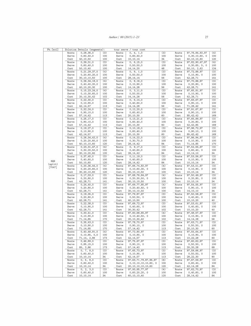
Author / 00 (2015) 1–23 27

Pb.[sol] Solution Details (segments): tour serve / tour cost

SQ9

(split)

[7047]

Route 0,28,36,0 (3)

Serve 0,60,40,0 100

Cost 40,10,50 100

Route 0,39,31,0 (3)

Serve 0,60,40,0 100

Cost 50,10,40 100

Route 0,21,29,37,0 (4)

Serve 0,20,60,20,0 100

Cost 30,10,10,50 100

Route 0,26,34,18,0 (4)

Serve 0,40,40,20,0 100

Cost 40,10,20,30 100

Route 0,15,23,24,0 (4)

Serve 0,10,30,60,0 100

Cost 20,10,30,42 102

Route 0,22,30,0 (3)

Serve 0,10,90,0 100

Cost 42,14,57 113

Route 0,32,24,0 (3)

Serve 0,90,10,0 100

Cost 57,14,42 113

Route 0,25,17,0 (3)

Serve 0,90,10,0 100

Cost 57,14,42 113

Route 0,19,27,0 (3)

Serve 0,10,90,0 100

Cost 42,14,57 113

Route 0,26,34,42,0 (4)

Serve 0,20,20,60,0 100

Cost 40,10,10,60 120

Route 0,23,31,47,0 (4)

Serve 0,30,20,50,0 100

Cost 30,10,20,60 120

Route 0,37,45,0 (3)

Serve 0,40,60,0 100

Cost 50,10,60 120

Route 0,20,36,44,0 (4)

Serve 0,20,20,60,0 100

Cost 30,20,10,60 120

Route 0,17,33,0 (3)

Serve 0,20,80,0 100

Cost 42,28,71 141

Route 0,24,40,0 (3)

Serve 0,20,80,0 100

Cost 42,28,71 141

Route 0,19,35,0 (3)

Serve 0,20,80,0 100

Cost 42,28,71 141

Route 0,22,38,0 (3)

Serve 0,10,90,0 100

Cost 42,28,71 141

Route 0,33,41,0 (3)

Serve 0,10,90,0 100

Cost 71,14,85 170

Route 0,35,43,0 (3)

Serve 0,10,90,0 100

Cost 71,14,85 170

Route 0,40,48,91,0 (4)

Serve 0,10,85, 5,0 100

Cost 71,14, 2,86 173

Route 0,46,89,0 (3)

Serve 0,85,15,0 100

Cost 85, 2,86 173

Route 0, 7, 8,0 (3)

Serve 0,60,40,0 100

Cost 10,10,14 34

Route 0, 5, 8,0 (3)

Serve 0,60,40,0 100

Cost 10,10,14 34

Route 0, 2, 3,0 (3)

Serve 0,60,40,0 100

Cost 10,10,14 34

Route 0, 4, 1,0 (3)

Serve 0,60,40,0 100

Cost 10,10,14 34

Route 0, 6,15,0 (3)

Serve 0,50,50,0 100

Cost 14,14,20 48

Route 0, 9, 1,0 (3)

Serve 0,50,50,0 100

Cost 28,14,14 56

Route 0, 8,16,0 (3)

Serve 0,10,90,0 100

Cost 14,14,28 56

Route 0, 3,11,0 (3)

Serve 0,50,50,0 100

Cost 14,14,28 56

Route 0, 6,14,0 (3)

Serve 0,40,60,0 100

Cost 14,14,28 56

Route 0,12,20,0 (3)

Serve 0,60,40,0 100

Cost 20,10,30 60

Route 0,13,21,0 (3)

Serve 0,60,40,0 100

Cost 20,10,30 60

Route 0,10,18,0 (3)

Serve 0,60,40,0 100

Cost 20,10,30 60

Route 0,14,22,0 (3)

Serve 0,30,70,0 100

Cost 28,14,42 84

Route 0, 9,17,0 (3)

Serve 0,40,60,0 100

Cost 28,14,42 84

Route 0,11,19,0 (3)

Serve 0,40,60,0 100

Cost 28,14,42 84

Route 97,66,74,82,97 (4)

Serve 0,10,60,30, 0 100

Cost 30,10,10,50 100

Route 97,68,76,84,97 (4)

Serve 0,20,30,50, 0 100

Cost 30,10,10,50 100

Route 97,69,77,85,97 (4)

Serve 0,20,40,40, 0 100

Cost 30,10,10,50 100

Route 97,79,87,97 (3)

Serve 0,50,50, 0 100

Cost 40,10,50 100

Route 97,69,72,97 (3)

Serve 0,40,60, 0 100

Cost 30,30,42 102

Route 97,60,68,65,97 (4)

Serve 0,10,40,50, 0 100

Cost 20,10,30,42 102

Route 97,78,70,97 (3)

Serve 0,90,10, 0 100

Cost 57,14,42 113

Route 97,72,80,97 (3)

Serve 0,10,90, 0 100

Cost 42,14,57 113

Route 97,75,67,97 (3)

Serve 0,90,10, 0 100

Cost 57,14,42 113

Route 97,65,73,97 (3)

Serve 0,10,90, 0 100

Cost 42,14,57 113

Route 97,63,71,79,87,95,97 (6)

Serve 0,10,10,10,10,60, 0 100

Cost 20,10,10,10,10,60 120

Route 97,93,85,77,97 (4)

Serve 0,60,20,20, 0 100

Cost 60,10,10,40 120

Route 97,76,84,92,97 (4)

Serve 0,30,10,60, 0 100

Cost 40,10,10,60 120

Route 97,82,90,47,97 (4)

Serve 0,30,65, 5, 0 100

Cost 50,10, 2,62 124

Route 97,72,88,97 (3)

Serve 0,10,90, 0 100

Cost 42,28,71 141

Route 97,70,86,97 (3)

Serve 0,20,80, 0 100

Cost 42,28,71 141

Route 97,65,81,97 (3)

Serve 0,10,90, 0 100

Cost 42,28,71 141

Route 97,83,67,97 (3)

Serve 0,90,10, 0 100

Cost 71,28,42 141

Route 97,91,67,97 (3)

Serve 0,90,10, 0 100

Cost 85,42,42 169

Route 97,65,89,97 (3)

Serve 0,20,80, 0 100

Cost 42,42,85 169

Route 97,96,72,97 (3)

Serve 0,90,10, 0 100

Cost 85,42,42 169

Route 97,86,94,97 (3)

Serve 0,10,90, 0 100

Cost 71,14,85 170

Route 97,52,55,97 (3)

Serve 0,60,40, 0 100

Cost 10,14,10 34

Route 97,53,56,97 (3)

Serve 0,10,90, 0 100

Cost 10,10,14 34

Route 97,53,51,97 (3)

Serve 0,10,90, 0 100

Cost 10,10,14 34

Route 97,50,49,97 (3)

Serve 0,20,80, 0 100

Cost 10,10,14 34

Route 97,54,55,97 (3)

Serve 0,90,10, 0 100

Cost 14,10,10 34

Route 97,50,58,97 (3)

Serve 0,40,60, 0 100

Cost 10,10,20 40

Route 97,53,61,97 (3)

Serve 0,40,60, 0 100

Cost 10,10,20 40

Route 97,49,57,97 (3)

Serve 0,10,90, 0 100

Cost 14,14,28 56

Route 97,63,71,97 (3)

Serve 0,50,50, 0 100

Cost 20,10,30 60

Route 97,55,64,97 (3)

Serve 0,10,90, 0 100

Cost 10,22,28 60

Route 97,60,62,97 (3)

Serve 0,50,50, 0 100

Cost 20,20,28 68

Route 97,59,66,97 (3)

Serve 0,50,50, 0 100

Cost 28,22,30 80

Route 97,67,59,97 (3)

Serve 0,60,40, 0 100

Cost 42,14,28 84

Route 97,62,70,97 (3)

Serve 0,40,60, 0 100

Cost 28,14,42 84

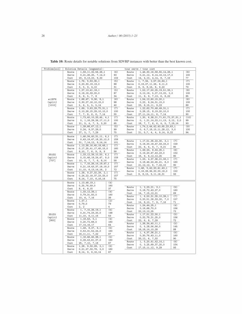
28 Author / 00 (2015) 1–23

Table 10: Route details for notable solutions from SDVRP instances with better than the best known cost.

Problem[sol] Solution Details (segments): tour serve / tour cost

eilB76

(split)

[1010]

Route 1,59,11,32,56,26,1 (6)

Serve 0,21,26,25, 7,14,0 93

Cost 20, 6,13,22, 9,33 103

Route 1,76, 5,53,35,1 (5)

Serve 0,20,30,19,19,0 88

Cost 3, 5, 9, 4,10 31

Route 1,27,13,41,18,1 (5)

Serve 0,18,16,33,20,0 87

Cost 6, 8, 5, 7, 8 34

Route 1,68,47, 9,36, 8,1 (6)

Serve 0,30,27,16,10,15,0 98

Cost 5, 6, 5, 5, 5,14 40

Route 1,69, 3,63,29,75,31,1 (7)

Serve 0,10,26,15,29,10,10,0 100

Cost 7, 7, 8, 6, 6, 7,14 55

Route 1,73,40,10,33,45, 4,1 (7)

Serve 0, 1,16,29,26,17,11,0 100

Cost 21, 5, 4, 7, 5, 3,20 65

Route 1,39,66,67,12,1 (5)

Serve 0,24, 9,37,29,0 99

Cost 27, 5, 7, 7,29 75

Route 1,46,30,16,58,55,14,28,1 (8)

Serve 0,21,12, 8,14,16,12,17,0 100

Cost 14, 4,10, 4,14, 8, 7,16 77

Route 1, 7,34, 2,57,24,64,1 (7)

Serve 0,19,27,11,26, 6,11,0 100

Cost 9, 9, 8,16, 6, 9,22 79

Route 1,52,17,50,25,19,51,33,1 (8)

Serve 0,12,19, 5,27,13,22, 2,0 100

Cost 11, 9, 9, 7,13, 6, 8,22 85

Route 1,54,12,60,15,20,1 (6)

Serve 0,22, 8,24,31,15,0 100

Cost 23, 8,15,11, 9,23 89

Route 1,22,62,70,48,49,31,1 (7)

Serve 0,28,15, 8,19,20,10,0 100

Cost 27,11,14,11, 6, 7,14 90

Route 1,30, 6,38,21,71,61,72,37,31,1 (10)

Serve 0, 1,21,14,22,11,13, 3,12, 2,0 99

Cost 18, 7, 7, 6, 6, 4, 5, 7,19,14 93

Route 1,74,2,44,42,43,65,23,63,1 (9)

Serve 0, 6,7,18,15,11,28,12, 3,0 100

Cost 21, 5,7, 4, 4, 9,14, 8,22 94

S51D2

(split)

[707]

Route 1,46,34,40,31,11, 6,1 (7)

Serve 0,43,19,47,18,20,12,0 159

Cost 31, 7,14,12, 9,14,14 101

Route 1,13,38,16,45,18,48,1 (7)

Serve 0,17,25,41,17,45,15,0 160

Cost 8,10, 7, 6, 9, 9, 9 58

Route 1,33,12,39,10,50, 6,1 (7)

Serve 0,15,46,18,24,47, 9,0 159

Cost 10, 6, 7, 7, 6, 8,14 58

Route 1, 7,15,26,14,19,47,1 (7)

Serve 0,21,19,43,37,18,19,0 157

Cost 11,10, 6,13,14,16, 2 72

Route 1,28, 9,27,32,29, 2,1 (7)

Serve 0,24,22,18,37,23,33,0 157

Cost 8,14, 7,10, 6,16,14 75

Route 1,17,51,35,22,30, 3,1 (7)

Serve 0,18,20,18,47,33,23,0 159

Cost 22, 6, 6, 9, 7, 9,21 80

Route 1,49,24, 8,44,25,1 (6)

Serve 0,19,20,47,43,23,0 152

Cost 16, 9, 6,12,12,25 80

Route 1,23, 4,37,36,21,33,1 (7)

Serve 0,18,46,22,45,21, 8,0 160

Cost 21,12,12, 6, 7,22,10 90

Route 1,48, 5,42,20,41,43,1 (7)

Serve 0,18,28,36,32,20,18,0 152

Cost 9, 8,13, 5,11,16,31 93

S51D3

(split)

[953]

Route 1,13,48,19,1 (4)

Serve 0,25,76,59,0 160

Cost 8, 6, 8,15 37

Route 1,33,12,39,1 (4)

Serve 0,79,31,50,0 160

Cost 10, 6, 7,16 39

Route 1,47,1 (2)

Serve 0,79,0 79

Cost 2, 2 4

Route 1, 7,15,26,19,1 (5)

Serve 0,31,74,23,20,0 148

Cost 11,10, 6,11,15 53

Route 1,18,43, 5,1 (4)

Serve 0,20,72,68,0 160

Cost 17,14,16,17 64

Route 1,49, 8,27, 9,1 (5)

Serve 0,53,31,52,24,0 160

Cost 16,11,11, 7,22 67

Route 1,16,46,45,38,1 (5)

Serve 0,29,43,61,27,0 160

Cost 25, 7,10, 7,18 67

Route 1,28, 9,32,29, 2,1 (6)

Serve 0,21,27,32,78, 2,0 160

Cost 8,14, 9, 6,16,14 67

Route 1, 2,23,21, 3,1 (5)

Serve 0,18,72,43,27,0 160

Cost 14, 7,15,12,21 69

Route 1, 6,50,31,35,10,39,1 (7)

Serve 0,20,51,26,33,20, 7,0 157

Cost 14, 8,10, 7, 9, 7,16 71

Route 1,24,44,25,1 (4)

Serve 0,18,68,70,0 156

Cost 22,13,12,25 72

Route 1,17,51,22,30,1 (5)

Serve 0,32,78,21,25,0 156

Cost 22, 6, 8, 7,29 72

Route 1,38,34,40,11,1 (5)

Serve 0, 5,28,56,56,0 145

Cost 18,18,14,10,28 88

Route 1, 4,37,36,21,1 (5)

Serve 0,30,76,43,11,0 160

Cost 33,12, 6, 7,32 90

Route 1, 5,20,41,42,14,1 (6)

Serve 0, 3,25,69,37,20,0 154

Cost 17,15,11,12, 9,29 93

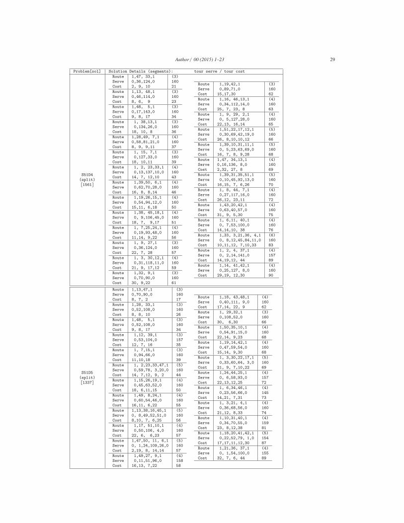
Author / 00 (2015) 1–23 29

Problem[sol] Solution Details (segments): tour serve / tour cost

S51D4

(split)

[1561]

Route 1,47, 33,1 (3)

Serve 0,36,124,0 160

Cost 2, 9, 10 21

Route 1,13, 48,1 (3)

Serve 0,46,114,0 160

Cost 8, 6, 9 23

Route 1,48, 5,1 (3)

Serve 0,17,143,0 160

Cost 9, 8, 17 34

Route 1, 38,13,1 (3)

Serve 0,134,26,0 160

Cost 18, 10, 8 36

Route 1,28,49, 7,1 (4)

Serve 0,58,81,21,0 160

Cost 8, 9, 9,11 37

Route 1, 15, 7,1 (3)

Serve 0,127,33,0 160

Cost 18, 10,11 39

Route 1, 2, 23,33,1 (4)

Serve 0,13,137,10,0 160

Cost 14, 7, 12,10 43

Route 1,39,50, 6,1 (4)

Serve 0,62,70,28,0 160

Cost 16, 8, 8,14 46

Route 1,19,26,15,1 (4)

Serve 0,54,94,12,0 160

Cost 15,11, 6,18 50

Route 1,38, 45,18,1 (4)

Serve 0, 9,106,45,0 160

Cost 18, 7, 9,17 51

Route 1, 7,25,24,1 (4)

Serve 0,19,93,48,0 160

Cost 11,14, 9,22 56

Route 1, 9, 27,1 (3)

Serve 0,36,124,0 160

Cost 22, 7, 28 57

Route 1, 3, 30,12,1 (4)

Serve 0,31,118,11,0 160

Cost 21, 9, 17,12 59

Route 1,32, 9,1 (3)

Serve 0,70,90,0 160

Cost 30, 9,22 61

Route 1,19,42,1 (3)

Serve 0,89,71,0 160

Cost 15,17,30 62

Route 1,16, 46,13,1 (4)

Serve 0,34,112,14,0 160

Cost 25, 7, 23, 8 63

Route 1, 9, 29, 2,1 (4)

Serve 0, 5,127,28,0 160

Cost 22,13, 16,14 65

Route 1,51,22,17,12,1 (5)

Serve 0,30,69,42,19,0 160

Cost 26, 8,10,10,12 66

Route 1,39,10,31,11,1 (5)

Serve 0, 5,23,63,69,0 160

Cost 16, 7, 8, 9,28 68

Route 1,47, 34,13,1 (4)

Serve 0,16,136, 8,0 160

Cost 2,32, 27, 8 69

Route 1,39,31,35,51,1 (5)

Serve 0,10,45,92,13,0 160

Cost 16,15, 7, 6,26 70

Route 1, 8, 44, 7,1 (4)

Serve 0,27,117,16,0 160

Cost 26,12, 23,11 72

Route 1,43,20,42,1 (4)

Serve 0,63,40,57,0 160

Cost 31, 9, 5,30 75

Route 1, 6,11, 40,1 (4)

Serve 0, 7,53,100,0 160

Cost 14,14,10, 38 76

Route 1,33, 3,21,36, 4,1 (6)

Serve 0, 8,12,45,84,11,0 160

Cost 10,11,12, 7,10,33 83

Route 1, 2, 4, 37,1 (4)

Serve 0, 2,14,141,0 157

Cost 14,19,12, 44 89

Route 1,14, 41,42,1 (4)

Serve 0,25,127, 8,0 160

Cost 29,19, 12,30 90

S51D5

(split)

[1337]

Route 1,13,47,1 (3)

Serve 0,70,90,0 160

Cost 8, 7, 2 17

Route 1,28, 33,1 (3)

Serve 0,52,108,0 160

Cost 8, 8, 10 26

Route 1,48, 5,1 (3)

Serve 0,52,108,0 160

Cost 9, 8, 17 34

Route 1,12, 39,1 (3)

Serve 0,53,104,0 157

Cost 12, 7, 16 35

Route 1, 7,15,1 (3)

Serve 0,94,66,0 160

Cost 11,10,18 39

Route 1, 2,23,33,47,1 (5)

Serve 0,59,78, 3,20,0 160

Cost 14, 7,12, 9, 2 44

Route 1,15,26,19,1 (4)

Serve 0,45,63,52,0 160

Cost 18, 6,11,15 50

Route 1,49, 8,24,1 (4)

Serve 0,60,54,46,0 160

Cost 16,11, 6,22 55

Route 1,13,38,16,45,1 (5)

Serve 0, 8,49,52,51,0 160

Cost 8,10, 7, 6,25 56

Route 1,17, 51,10,1 (4)

Serve 0,50,106, 4,0 160

Cost 22, 6, 6,23 57

Route 1,47,50, 11, 6,1 (5)

Serve 0, 1,24,109,26,0 160

Cost 2,19, 8, 14,14 57

Route 1,49,27, 9,1 (4)

Serve 0,11,51,96,0 158

Cost 16,13, 7,22 58

Route 1,18, 43,48,1 (4)

Serve 0,40,111, 9,0 160

Cost 17,14, 22, 9 62

Route 1, 29,32,1 (3)

Serve 0,108,52,0 160

Cost 30, 6,30 66

Route 1,50,35,10,1 (4)

Serve 0,54,91,15,0 160

Cost 22,14, 9,23 68

Route 1,19,14,42,1 (4)

Serve 0,47,59,54,0 160

Cost 15,14, 9,30 68

Route 1, 3,30,22,17,1 (5)

Serve 0,33,60,64, 3,0 160

Cost 21, 9, 7,10,22 69

Route 1,24,44,25,1 (4)

Serve 0, 6,58,93,0 157

Cost 22,13,12,25 72

Route 1, 6,34,46,1 (4)

Serve 0,23,56,66,0 145

Cost 14,21, 7,31 73

Route 1, 3,21, 4,1 (4)

Serve 0,36,68,56,0 160

Cost 21,12, 8,33 74

Route 1,10,31,40,1 (4)

Serve 0,34,70,55,0 159

Cost 23, 8,12,38 81

Route 1,18,20,41,42,1 (5)

Serve 0,22,52,79, 1,0 154

Cost 17,17,11,12,30 87

Route 1,21,36, 37,1 (4)

Serve 0, 1,54,100,0 155

Cost 32, 7, 6, 44 89

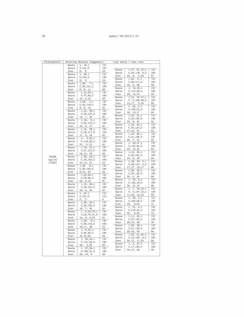
30 Author / 00 (2015) 1–23

Problem[sol] Solution Details (segments): tour serve / tour cost

S51D6

(split)

[2182]

Route 1, 13,1 (2)

Serve 0,131,0 131

Cost 8, 8 16

Route 1, 48,1 (2)

Serve 0,140,0 140

Cost 9, 9 18

Route 1,28, 7,1 (3)

Serve 0,39,121,0 160

Cost 8, 9, 11 28

Route 1,12,33,1 (3)

Serve 0,77,83,0 160

Cost 12, 6,10 28

Route 1,28, 2,1 (3)

Serve 0,42,118,0 160

Cost 8, 8, 14 30

Route 1,12, 39,1 (3)

Serve 0,33,127,0 160

Cost 12, 7, 16 35

Route 1,19, 5,1 (3)

Serve 0,50,110,0 160

Cost 15, 8, 17 40

Route 1,18, 38,1 (3)

Serve 0,36,117,0 153

Cost 17, 5, 18 40

Route 1, 3,33,1 (3)

Serve 0,118,42,0 160

Cost 21, 11,10 42

Route 1,19, 15,1 (3)

Serve 0,47,113,0 160

Cost 15,10, 18 43

Route 1,33, 23,1 (3)

Serve 0,18,142,0 160

Cost 10,12, 21 43

Route 1,28, 9,1 (3)

Serve 0,20,140,0 160

Cost 8,14, 22 44

Route 1,24,49,1 (3)

Serve 0,78,82,0 160

Cost 22, 9,16 47

Route 1,15, 26,1 (3)

Serve 0,29,131,0 160

Cost 18, 6, 23 47

Route 1, 47,1 (2)

Serve 0,121,0 121

Cost 2, 2 4

Route 1,38, 45,1 (3)

Serve 0,26,134,0 160

Cost 18, 7, 25 50

Route 1, 6,50,10,1 (4)

Serve 0,33,76,51,0 160

Cost 14, 8, 6,23 51

Route 1,49, 8,1 (3)

Serve 0,46,114,0 160

Cost 16,11, 26 53

Route 1, 6,16,1 (3)

Serve 0,65,95,0 160

Cost 14,15,25 54

Route 1, 25,24,1 (3)

Serve 0,131,29,0 160

Cost 25, 9,22 56

Route 1, 27,28,1 (3)

Serve 0,139,21,0 160

Cost 28, 20, 8 56

Route 1,17, 51,10,1 (4)

Serve 0,34,118, 8,0 160

Cost 22, 6, 6,23 57

Route 1,50, 11,1 (3)

Serve 0,49,111,0 160

Cost 22, 8, 28 58

Route 1, 14,19,1 (3)

Serve 0,114,46,0 160

Cost 29, 14,15 58

Route 1,12, 30,17,1 (4)

Serve 0, 5,106,49,0 160

Cost 12,17, 9,22 60

Route 1, 42, 5,1 (3)

Serve 0,129,31,0 160

Cost 30, 13,17 60

Route 1,10, 31,1 (3)

Serve 0,25,135,0 160

Cost 23, 8, 31 62

Route 1,18, 43,1 (3)

Serve 0,35,123,0 158

Cost 17,14, 31 62

Route 1,16, 46,1 (3)

Serve 0,21,136,0 157

Cost 25, 7, 31 63

Route 1, 22,17,1 (3)

Serve 0,125,35,0 160

Cost 32, 10,22 64

Route 1,10, 35,1 (3)

Serve 0,29,131,0 160

Cost 23, 9, 32 64

Route 1,18, 20, 5,1 (4)

Serve 0,48,110, 2,0 160

Cost 17,17, 15,17 66

Route 1,29, 32,1 (3)

Serve 0,35,125,0 160

Cost 30, 6, 30 66

Route 1, 34, 6,1 (3)

Serve 0,142,18,0 160

Cost 34, 21,14 69

Route 1, 7, 44,24,1 (4)

Serve 0, 9,137,13,0 159

Cost 11,23, 13,22 69

Route 1, 29, 4,1 (3)

Serve 0,104,56,0 160

Cost 30, 9,33 72

Route 1, 21, 4,1 (3)

Serve 0,119,41,0 160

Cost 32, 8,33 73

Route 1,11, 40,1 (3)

Serve 0,27,133,0 160

Cost 28,10, 38 76

Route 1,30, 36,1 (3)

Serve 0,31,129,0 160

Cost 29,16, 39 84

Route 1,42, 41,20,1 (4)

Serve 0,13,139, 8,0 160

Cost 30,12, 11,32 85

Route 1, 4, 37,1 (3)

Serve 0,17,143,0 160

Cost 33,12, 44 89

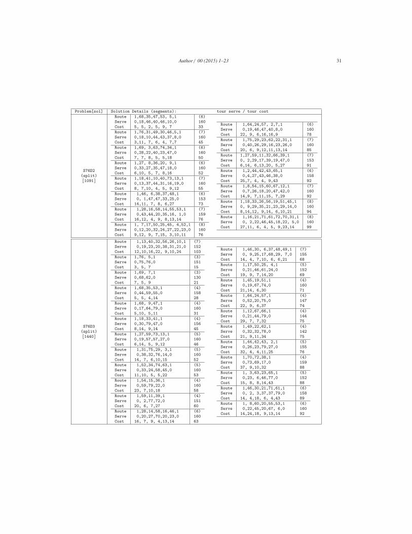
Author / 00 (2015) 1–23 31

Problem[sol] Solution Details (segments): tour serve / tour cost

S76D2

(split)

[1091]

Route 1,68,35,47,53, 5,1 (6)

Serve 0,18,46,40,46,10,0 160

Cost 5, 5, 2, 5, 9, 7 33

Route 1,76,31,49,30,46,5,1 (7)

Serve 0,18,10,44,43,37,8,0 160

Cost 3,11, 7, 6, 4, 7,7 45

Route 1,69, 3,63,74,34,1 (6)

Serve 0,28,22,40,23,47,0 160

Cost 7, 7, 8, 5, 5,18 50

Route 1,27, 8,36,20, 9,1 (6)

Serve 0,33,27,35,47,18,0 160

Cost 6,10, 5, 7, 8,16 52

Route 1,18,41,10,40,73,13,1 (7)

Serve 0,13,37,44,31,16,19,0 160

Cost 8, 7,10, 4, 5, 9,12 55

Route 1,46, 6,38,37,48,1 (6)

Serve 0, 1,47,47,33,25,0 153

Cost 14,11, 7, 8, 6,27 73

Route 1,28,16,58,14,55,53,1 (7)

Serve 0,43,44,20,35,16, 1,0 159

Cost 16,12, 4, 9, 8,13,14 76

Route 1, 7,17,50,25,45, 4,52,1 (8)

Serve 0,12,20,32,24,27,22,23,0 160

Cost 9,12, 9, 7,15, 3,10,11 76

Route 1,64,24,57, 2,7,1 (6)

Serve 0,19,46,47,40,8,0 160

Cost 22, 9, 6,16,16,9 78

Route 1,75,29,23,62,22,31,1 (7)

Serve 0,40,26,29,16,23,26,0 160

Cost 20, 6, 9,12,11,13,14 85

Route 1,27,59,11,32,66,39,1 (7)

Serve 0, 2,29,17,39,19,47,0 153

Cost 6,14, 6,13,20, 5,27 91

Route 1,2,44,42,43,65,1 (6)

Serve 0,4,27,43,46,38,0 158

Cost 25,7, 4, 4, 9,43 92

Route 1,8,54,15,60,67,12,1 (7)

Serve 0,7,26,18,20,47,42,0 160

Cost 14,9, 7,11,15, 7,29 92

Route 1,18,33,26,56,19,51,45,1 (8)

Serve 0, 9,29,35,21,23,29,14,0 160

Cost 8,14,12, 9,14, 6,10,21 94

Route 1,16,21,71,61,72,70,31,1 (8)

Serve 0, 2,22,46,45,18,22, 5,0 160

Cost 27,11, 6, 4, 5, 9,23,14 99

S76D3

(split)

[1440]

Route 1,13,40,32,56,26,10,1 (7)

Serve 0,19,23,20,38,31,21,0 152

Cost 12,10,16,22, 9,10,24 103

Route 1,76, 5,1 (3)

Serve 0,75,76,0 151

Cost 3, 5, 7 15

Route 1,69, 7,1 (3)

Serve 0,68,62,0 130

Cost 7, 5, 9 21

Route 1,68,35,53,1 (4)

Serve 0,44,59,55,0 158

Cost 5, 5, 4,14 28

Route 1,68, 9,47,1 (4)

Serve 0,17,64,79,0 160

Cost 5,10, 5,11 31

Route 1,18,33,41,1 (4)

Serve 0,30,79,47,0 156

Cost 8,14, 9,14 45

Route 1,27,59,73,13,1 (5)

Serve 0,19,57,57,27,0 160

Cost 6,14, 5, 9,12 46

Route 1,31,75,29, 3,1 (5)

Serve 0,38,32,76,14,0 160

Cost 14, 7, 6,10,15 52

Route 1,52,34,74,63,1 (5)

Serve 0,33,24,58,45,0 160

Cost 11,10, 5, 5,22 53

Route 1,54,15,36,1 (4)

Serve 0,59,79,22,0 160

Cost 23, 7,10,18 58

Route 1,59,11,39,1 (4)

Serve 0, 2,77,72,0 151

Cost 20, 6, 7,27 60

Route 1,28,14,58,16,46,1 (6)

Serve 0,20,27,70,20,23,0 160

Cost 16, 7, 9, 4,13,14 63

Route 1,46,30, 6,37,48,49,1 (7)

Serve 0, 9,25,17,68,29, 7,0 155

Cost 14, 4, 7,10, 6, 6,21 68

Route 1,17,50,25, 4,1 (5)

Serve 0,21,46,61,24,0 152

Cost 19, 9, 7,14,20 69

Route 1,45,19,51,1 (4)

Serve 0,19,67,74,0 160

Cost 21,14, 6,30 71

Route 1,64,24,57,1 (4)

Serve 0,52,20,75,0 147

Cost 22, 9, 6,37 74

Route 1,12,67,66,1 (4)

Serve 0,21,44,79,0 144

Cost 29, 7, 7,32 75

Route 1,49,22,62,1 (4)

Serve 0,32,32,78,0 142

Cost 21, 9,11,34 75

Route 1,44,42,43, 2,1 (5)

Serve 0,26,23,79,27,0 155

Cost 32, 4, 4,11,25 76

Route 1,70,72,38,1 (4)

Serve 0,73,69,17,0 159

Cost 37, 9,10,32 88

Route 1, 3,63,23,65,1 (5)

Serve 0,23, 6,46,77,0 152

Cost 15, 8, 8,14,43 88

Route 1,46,30,21,71,61,1 (6)

Serve 0, 2, 3,37,37,79,0 158

Cost 14, 4,18, 6, 4,43 89

Route 1, 8,60,20,55,53,1 (6)

Serve 0,22,45,20,67, 6,0 160

Cost 14,24,18, 9,13,14 92

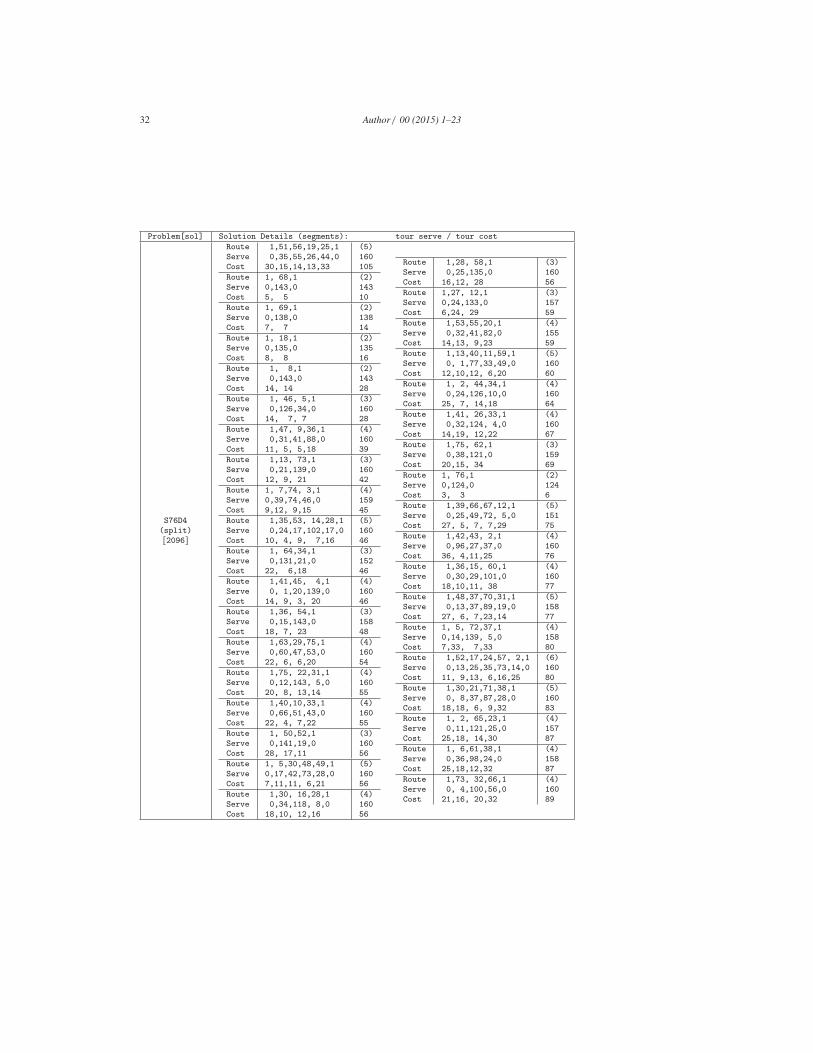
32 Author / 00 (2015) 1–23

Problem[sol] Solution Details (segments): tour serve / tour cost

S76D4

(split)

[2096]

Route 1,51,56,19,25,1 (5)

Serve 0,35,55,26,44,0 160

Cost 30,15,14,13,33 105

Route 1, 68,1 (2)

Serve 0,143,0 143

Cost 5, 5 10

Route 1, 69,1 (2)

Serve 0,138,0 138

Cost 7, 7 14

Route 1, 18,1 (2)

Serve 0,135,0 135

Cost 8, 8 16

Route 1, 8,1 (2)

Serve 0,143,0 143

Cost 14, 14 28

Route 1, 46, 5,1 (3)

Serve 0,126,34,0 160

Cost 14, 7, 7 28

Route 1,47, 9,36,1 (4)

Serve 0,31,41,88,0 160

Cost 11, 5, 5,18 39

Route 1,13, 73,1 (3)

Serve 0,21,139,0 160

Cost 12, 9, 21 42

Route 1, 7,74, 3,1 (4)

Serve 0,39,74,46,0 159

Cost 9,12, 9,15 45

Route 1,35,53, 14,28,1 (5)

Serve 0,24,17,102,17,0 160

Cost 10, 4, 9, 7,16 46

Route 1, 64,34,1 (3)

Serve 0,131,21,0 152

Cost 22, 6,18 46

Route 1,41,45, 4,1 (4)

Serve 0, 1,20,139,0 160

Cost 14, 9, 3, 20 46

Route 1,36, 54,1 (3)

Serve 0,15,143,0 158

Cost 18, 7, 23 48

Route 1,63,29,75,1 (4)

Serve 0,60,47,53,0 160

Cost 22, 6, 6,20 54

Route 1,75, 22,31,1 (4)

Serve 0,12,143, 5,0 160

Cost 20, 8, 13,14 55

Route 1,40,10,33,1 (4)

Serve 0,66,51,43,0 160

Cost 22, 4, 7,22 55

Route 1, 50,52,1 (3)

Serve 0,141,19,0 160

Cost 28, 17,11 56

Route 1, 5,30,48,49,1 (5)

Serve 0,17,42,73,28,0 160

Cost 7,11,11, 6,21 56

Route 1,30, 16,28,1 (4)

Serve 0,34,118, 8,0 160

Cost 18,10, 12,16 56

Route 1,28, 58,1 (3)

Serve 0,25,135,0 160

Cost 16,12, 28 56

Route 1,27, 12,1 (3)

Serve 0,24,133,0 157

Cost 6,24, 29 59

Route 1,53,55,20,1 (4)

Serve 0,32,41,82,0 155

Cost 14,13, 9,23 59

Route 1,13,40,11,59,1 (5)

Serve 0, 1,77,33,49,0 160

Cost 12,10,12, 6,20 60

Route 1, 2, 44,34,1 (4)

Serve 0,24,126,10,0 160

Cost 25, 7, 14,18 64

Route 1,41, 26,33,1 (4)

Serve 0,32,124, 4,0 160

Cost 14,19, 12,22 67

Route 1,75, 62,1 (3)

Serve 0,38,121,0 159

Cost 20,15, 34 69

Route 1, 76,1 (2)

Serve 0,124,0 124

Cost 3, 3 6

Route 1,39,66,67,12,1 (5)

Serve 0,25,49,72, 5,0 151

Cost 27, 5, 7, 7,29 75

Route 1,42,43, 2,1 (4)

Serve 0,96,27,37,0 160

Cost 36, 4,11,25 76

Route 1,36,15, 60,1 (4)

Serve 0,30,29,101,0 160

Cost 18,10,11, 38 77

Route 1,48,37,70,31,1 (5)

Serve 0,13,37,89,19,0 158

Cost 27, 6, 7,23,14 77

Route 1, 5, 72,37,1 (4)

Serve 0,14,139, 5,0 158

Cost 7,33, 7,33 80

Route 1,52,17,24,57, 2,1 (6)

Serve 0,13,25,35,73,14,0 160

Cost 11, 9,13, 6,16,25 80

Route 1,30,21,71,38,1 (5)

Serve 0, 8,37,87,28,0 160

Cost 18,18, 6, 9,32 83

Route 1, 2, 65,23,1 (4)

Serve 0,11,121,25,0 157

Cost 25,18, 14,30 87

Route 1, 6,61,38,1 (4)

Serve 0,36,98,24,0 158

Cost 25,18,12,32 87

Route 1,73, 32,66,1 (4)

Serve 0, 4,100,56,0 160

Cost 21,16, 20,32 89

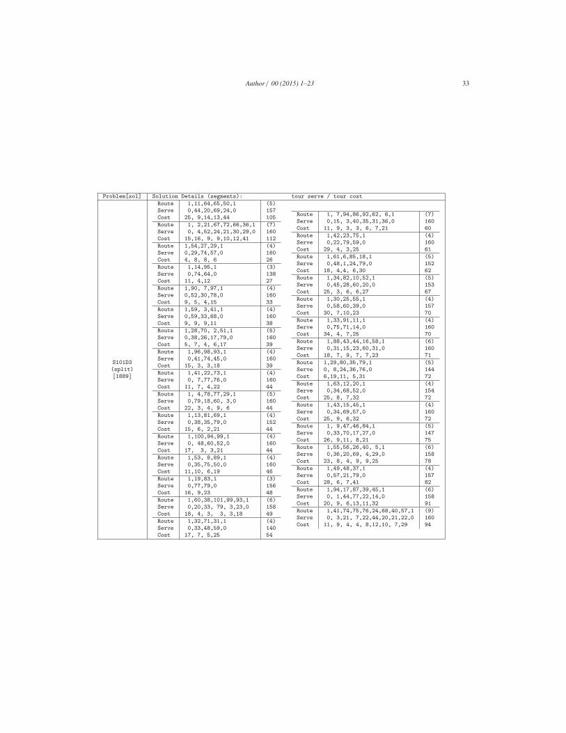
Author / 00 (2015) 1–23 33

Problem[sol] Solution Details (segments): tour serve / tour cost

S101D3

(split)

[1889]

Route 1,11,64,65,50,1 (5)

Serve 0,44,20,69,24,0 157

Cost 25, 9,14,13,44 105

Route 1, 2,21,67,72,66,36,1 (7)

Serve 0, 4,52,24,21,30,29,0 160

Cost 15,16, 9, 9,10,12,41 112

Route 1,54,27,29,1 (4)

Serve 0,29,74,57,0 160

Cost 4, 8, 8, 6 26

Route 1,14,95,1 (3)

Serve 0,74,64,0 138

Cost 11, 4,12 27

Route 1,90, 7,97,1 (4)

Serve 0,52,30,78,0 160

Cost 9, 5, 4,15 33

Route 1,59, 3,41,1 (4)

Serve 0,59,33,68,0 160

Cost 9, 9, 9,11 38

Route 1,28,70, 2,51,1 (5)

Serve 0,38,26,17,79,0 160

Cost 5, 7, 4, 6,17 39

Route 1,96,98,93,1 (4)

Serve 0,41,74,45,0 160

Cost 15, 3, 3,18 39

Route 1,41,22,73,1 (4)

Serve 0, 7,77,76,0 160

Cost 11, 7, 4,22 44

Route 1, 4,78,77,29,1 (5)

Serve 0,79,18,60, 3,0 160

Cost 22, 3, 4, 9, 6 44

Route 1,13,81,69,1 (4)

Serve 0,38,35,79,0 152

Cost 15, 6, 2,21 44

Route 1,100,94,99,1 (4)

Serve 0, 48,60,52,0 160

Cost 17, 3, 3,21 44

Route 1,53, 8,89,1 (4)

Serve 0,35,75,50,0 160

Cost 11,10, 6,19 46

Route 1,19,83,1 (3)

Serve 0,77,79,0 156

Cost 16, 9,23 48

Route 1,60,38,101,99,93,1 (6)

Serve 0,20,33, 79, 3,23,0 158

Cost 18, 4, 3, 3, 3,18 49

Route 1,32,71,31,1 (4)

Serve 0,33,48,59,0 140

Cost 17, 7, 5,25 54

Route 1, 7,94,86,92,62, 6,1 (7)

Serve 0,15, 3,40,35,31,36,0 160

Cost 11, 9, 3, 3, 6, 7,21 60

Route 1,42,23,75,1 (4)

Serve 0,22,79,59,0 160

Cost 29, 4, 3,25 61

Route 1,61,6,85,18,1 (5)

Serve 0,48,1,24,79,0 152

Cost 18, 4,4, 6,30 62

Route 1,34,82,10,52,1 (5)

Serve 0,45,28,60,20,0 153

Cost 25, 3, 6, 6,27 67

Route 1,30,25,55,1 (4)

Serve 0,58,60,39,0 157

Cost 30, 7,10,23 70

Route 1,33,91,11,1 (4)

Serve 0,75,71,14,0 160

Cost 34, 4, 7,25 70

Route 1,88,43,44,16,58,1 (6)

Serve 0,31,15,23,60,31,0 160

Cost 18, 7, 9, 7, 7,23 71

Route 1,29,80,35,79,1 (5)

Serve 0, 8,24,36,76,0 144

Cost 6,19,11, 5,31 72

Route 1,63,12,20,1 (4)

Serve 0,34,68,52,0 154

Cost 25, 8, 7,32 72

Route 1,43,15,45,1 (4)

Serve 0,34,69,57,0 160

Cost 25, 9, 6,32 72

Route 1, 9,47,46,84,1 (5)

Serve 0,33,70,17,27,0 147

Cost 26, 9,11, 8,21 75

Route 1,55,56,26,40, 5,1 (6)

Serve 0,36,20,69, 4,29,0 158

Cost 23, 8, 4, 9, 9,25 78

Route 1,49,48,37,1 (4)

Serve 0,57,21,79,0 157

Cost 28, 6, 7,41 82

Route 1,94,17,87,39,45,1 (6)

Serve 0, 1,44,77,22,14,0 158

Cost 20, 9, 6,13,11,32 91

Route 1,41,74,75,76,24,68,40,57,1 (9)

Serve 0, 3,21, 7,22,44,20,21,22,0 160

Cost 11, 9, 4, 4, 8,12,10, 7,29 94

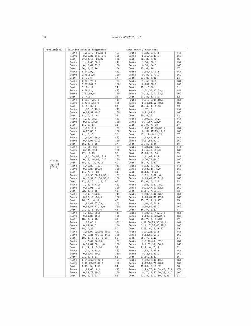
34 Author / 00 (2015) 1–23

Problem[sol] Solution Details (segments): tour serve / tour cost

S101D5

(split)

[2814]

Route 1,52,72, 66,21,1 (5)

Serve 0,16,27,111, 6,0 160

Cost 27,13,10, 21,32 103

Route 1,12,65,50,1 (4)

Serve 0,16,61,83,0 160

Cost 34,13,13,44 104

Route 1,54,29,1 (3)

Serve 0,76,84,0 160

Cost 4, 7, 6 17

Route 1,28, 70,1 (3)

Serve 0,53,107,0 160

Cost 5, 7, 12 24

Route 1,59,41,1 (3)

Serve 0,91,69,0 160

Cost 9, 4,11 24

Route 1,90, 7,95,1 (4)

Serve 0,77,31,52,0 160

Cost 9, 5, 3,12 29

Route 1,27,13,29,1 (4)

Serve 0,84,57,19,0 160

Cost 11, 7, 9, 6 33

Route 1,14, 98,1 (3)

Serve 0,52,108,0 160

Cost 11, 6, 17 34

Route 1,53,19,1 (3)

Serve 0,77,83,0 160

Cost 11, 8,16 35

Route 1,97,60,96,1 (4)

Serve 0,46,93,21,0 160

Cost 15, 3, 4,15 37

Route 1, 51, 2,1 (3)

Serve 0,108,52,0 160

Cost 17, 6,15 38

Route 1,97,100,94, 7,1 (5)

Serve 0, 6, 46,98,10,0 160

Cost 15, 2, 3, 9,11 40

Route 1,41,22, 74,1 (4)

Serve 0,32,23,105,0 160

Cost 11, 7, 3, 20 41

Route 1,95,96,38,99,93,1 (6)

Serve 0,10,31,31,38,50,0 160

Cost 12, 3, 6, 1, 3,18 43

Route 1, 4,78,77,1 (4)

Serve 0,62,91, 7,0 160

Cost 22, 3, 4,16 45

Route 1,19, 84,61,1 (4)

Serve 0,28,101,31,0 160

Cost 16, 7, 4,18 45

Route 1,81,69,77,29,1 (5)

Serve 0,53,57,47, 3,0 160

Cost 21, 2, 8, 9, 6 46

Route 1, 3,58,88,1 (4)

Serve 0,59,86,15,0 160

Cost 18, 6, 7,18 49

Route 1,88,43,1 (3)

Serve 0,69,91,0 160

Cost 18, 7,25 50

Route 1,93,99,92,101,38,1 (6)

Serve 0, 2,21,70, 53,14,0 160

Cost 18, 3, 4, 3, 3,21 52

Route 1, 7,62,86,60,1 (5)

Serve 0,22,87,50, 1,0 160

Cost 11,14, 4, 5,18 52

Route 1,71,11,32,1 (4)

Serve 0,56,64,40,0 160

Cost 21, 8, 8,17 54

Route 1,54,76,73,22,1 (5)

Serve 0,15,92,23,30,0 160

Cost 4,23, 5, 4,18 54

Route 1,89,63, 8,1 (4)

Serve 0,52,79,29,0 160

Cost 19, 6, 9,21 55

Route 1,73,75,23,1 (4)

Serve 0,25,48,87,0 160

Cost 22, 3, 3,27 55

Route 1,34, 80,1 (3)

Serve 0,56,104,0 160

Cost 25, 6, 26 57

Route 1,84,46, 9,1 (4)

Serve 0, 8,75,77,0 160

Cost 21, 8, 6,26 61

Route 1, 55,56,1 (3)

Serve 0,102,58,0 160

Cost 23, 8,30 61

Route 1,51,34,82,52,1 (5)

Serve 0, 2, 4,71,83,0 160

Cost 17, 8, 3, 7,27 62

Route 1,61, 6,85,18,1 (5)

Serve 0,34,21,52,52,0 159

Cost 18, 4, 4, 6,30 62

Route 1,57, 5,1 (3)

Serve 0,71,89,0 160

Cost 29, 8,25 62

Route 1,69,30, 25,1 (4)

Serve 0, 1,57,102,0 160

Cost 21, 9, 7, 30 67

Route 1,100,17,45,38,1 (5)

Serve 0, 31,17,93,19,0 160

Cost 17, 12, 6,11,21 67

Route 1,83,49,48,1 (4)

Serve 0,17,53,90,0 160

Cost 23, 5, 6,34 68

Route 1,70,31, 33,1 (4)

Serve 0, 4,45,111,0 160

Cost 12,13,10, 34 69

Route 1,11,64,91,1 (4)

Serve 0,24,72,64,0 160

Cost 25, 9, 4,32 70

Route 1,83, 47, 9,1 (4)

Serve 0,43,111, 6,0 160

Cost 23,13, 9,26 71

Route 1,62,17,87, 6,1 (5)

Serve 0,19,47,63,31,0 160

Cost 25, 4, 6,16,21 72

Route 1,32,12,20, 8,1 (5)

Serve 0,24,47,57,32,0 160

Cost 17,17, 7,11,21 73

Route 1,58,16,42,23,1 (5)

Serve 0,13,61,69,17,0 160

Cost 23, 7,12, 4,27 73

Route 1,40,26,56,1 (4)

Serve 0,56,55,49,0 160

Cost 34, 9, 4,30 77

Route 1,88,43, 44,15,1 (5)

Serve 0,10,13,100,37,0 160

Cost 18, 7, 9, 11,32 77

Route 1,29,80,79,35,10,1 (6)

Serve 0, 4, 7,55,65,29,0 160

Cost 6,19, 6, 5,11,32 79

Route 1,31,21,67,1 (4)

Serve 0,13,80,67,0 160

Cost 25, 7, 9,40 81

Route 1,8,49,48, 37,1 (5)

Serve 0,2,32,18,108,0 160

Cost 21,7, 6, 7, 41 82

Route 1,98,15,39,1 (4)

Serve 0, 2,69,89,0 160

Cost 17,15,11,42 85

Route 1,52,72,36,10,1 (5)

Serve 0,12,50,75,23,0 160

Cost 27,13, 7, 9,32 88

Route 1,73,76,24,68,40, 5,1 (7)

Serve 0, 7, 7,50,50,32,14,0 160

Cost 22, 5, 8,12,10, 9,25 91