The Multi-Depot Vehicle Routing Problem with Inter-Depot Routes

Benoit Crevier, Jean-Francois Cordeau and Gilbert Laporte

Canada Research Chair in Distribution Management

HEC Montreal

3000 chemin de la Cote-Sainte-Catherine

Montreal, Canada H3T 2A7

May 2005

Abstract

This article addresses an extension of the multi-depot vehicle routing problem in which vehicles may

be replenished at intermediate depots along their route. It proposes a heuristic combining the adaptative

memory principle, a tabu search method for the solution of subproblems, and integer programming. Tests

are conducted on randomly generated instances.

Keywords: multi-depot vehicle routing problem, replenishment, adaptative memory, tabu search, integer program-

ming.

1 Introduction

We study a variant of the multi-depot vehicle routing problem where depots can act as intermediate replen-

ishment facilities along the route of a vehicle. This problem is a generalization of the Vehicle Routing Problem

(VRP). The classical version of the VRP is defined on a graph G = (Vc ∪ Vd, A), where Vc = {v1, v2, . . . , vn}is the customer set, Vd = {vn+1} is the depot set and A = {(vi, vj) : vi, vj ∈ Vc∪Vd, i 6= j} is the arc set of G.

A fleet of m vehicles of capacity Q is located at vn+1. Each customer has a demand qi and a service duration

di. A cost or travel time cij is associated with every arc of the graph. The VRP consists of determining m

routes of minimal cost satisfying the following conditions: (i) every customer appears on exactly one route;

(ii) every route starts and ends at the depot; (iii) the total demand of the customers on any route does not

exceed Q; (iv) the total duration of a route does not exceed a preset value D.

1

Several algorithms are available for the VRP. Because this is a hard combinatorial problem, exact methods

tend to perform poorly on large size instances, which is why numerous heuristics have been developed.

These include classical heuristics such as construction and improvement procedures or two-phase approaches,

and metaheuristics like simulated annealing, tabu search, variable neighborhood search and evolutionary

algorithms. For surveys see Laporte and Semet [22], Gendreau, Laporte and Potvin [15] and Cordeau et al.

[8].

In some contexts, one can assign more than one route to a vehicle. The Vehicle Routing Problem with

Multiple Use of Vehicles (VRPM) is encountered, for example, when the vehicle fleet is small or when the

length of the day is large with respect to the average duration of a route. Fleischmann [12] was probably

the first to propose a heuristic for this problem. It is based on the savings principle for route construction

combined with a bin packing procedure for the assignment of routes to vehicles. Taillard, Laporte and

Gendreau [29] have developed an adaptative memory and a tabu search heuristic, again using a bin packing

procedure for assigning routes to vehicles. Other heuristics have been proposed for the VRPM, such as those

of Brandao and Mercer [3] [4] or Zhao et al. [34] based on tabu search or, in the ship routing context, the

methods proposed by Suprayogi, Yamato and Iskendar [28] and Fagerholt [11] which create routes by solving

traveling salesman problems (TSPs) and solve an integer program (Suprayogi, Yamato and Iskendar propose

a set partitioning problem) for the assignment part.

Another well-known generalization of the VRP is the Multi-Depot Vehicle Routing Problem (MDVRP). In

this extension every customer is visited by a vehicle based at one of several depots. In the standard MDVRP

every vehicle route must start and end at the same depot. There exist only a few exact algorithms for this

problem. Laporte, Nobert and Arpin [20] as well as Laporte, Nobert and Taillefer [21] have developed exact

branch-and-bound algorithms but, as mentionned earlier, these only work well on relatively small instances.

Several heuristics have been put forward for the MDVRP. Early heuristics based on simple construction and

improvement procedures have been developed by Tillman [30], Tillman and Hering [32], Tillman and Cain

[31], Wren and Holliday [33], Gillett and Johnson [16], Golden, Magnanti and Nguyen [17], and Raft [24].

More recently, Chao, Golden and Wasil [6] have proposed a search procedure combining Dueck’s [10] record-

to-record local method for the reassignment of customers to different vehicle routes, followed by Lin’s 2-opt

procedure [23] for the improvement of individual routes. Renaud, Boctor and Laporte [26] describe a tabu

search heuristic in which an initial solution is built by first assigning every customer to its nearest depot.

A petal algorithm developed by the same authors [25] is then used for the solution of the VRP associated

with each depot. It finally applies an improvement phase using either a subset of the 4-opt exchanges

to improve individual routes, swapping customers between routes from the same or different depots, or

exchanging customers between three routes. The tabu search approach of Cordeau, Gendreau and Laporte

[7] is probably the best known algorithm for the MDVRP. An initial solution is obtained by assigning each

2

customer to its nearest depot and a VRP solution is generated for each depot by means of a sweep algorithm.

Improvements are performed by transferring a customer between two routes incident to the same depot, or

by relocating a customer in a route incident to another depot. Reinsertions are performed by means of the

GENI heuristic [13]. One of the main characteristics of this algorithm is that infeasible solutions are allowed

throughout the search. Continuous diversification is achieved through the penalization of frequent moves.

The Multi-Depot Vehicle Routing Problem with Inter-Depot Routes (MDVRPI) has not received much

attention from researchers. A simplified version of the problem is discussed by Jordan and Burns [19] and

by Jordan [18] who assume that customer demands are all equal to Q and that inter-depot routes consist

of back-and-forth routes between two depots. The authors transform the problem into a matching problem

which is solved by a greedy algorithm. Angelelli and Speranza [2] have developed a heuristic for a version of

the Periodic Vehicle Routing Problem (PVRP) in which replenishments at intermediate facilities are allowed.

Their algorithm is based on the tabu search heuristic of Cordeau, Gendreau and Laporte [7]. A version of

the problem where time windows are considered is proposed by Cano Sevilla and Simon de Blas [5]. The

algorithm is based on neural networks and on an ant colony system.

Our interest in the MDVRPI arises from a real-life grocery distribution problem in the Montreal area.

Several similar applications are encountered in the context where the route of a vehicle can be composed of

multiple stops at intermediate depots in order for the vehicle to be replenished. When trucks and trailers are

used, the replenishment can be done by a switch of trailers. Angelelli and Speranza [1] present an application

of a similar problem in the context of waste collection.

Our aim is to develop a heuristic for the MDVRPI and to introduce a set of benchmark instances for

this problem. The remainder of this article is organized as follows. The problem is formulated in Section

2 and the heuristic is described in Section 3. Computational results are presented in Section 4, followed by

the conclusion in Section 5.

2 Formulation

The MDVRPI can be formulated as follows. Let G = (Vc∪Vd, A) be a directed graph where Vc = {v1, . . . , vn}is the customer set, Vd = {vn+1, vn+2, . . . , vn+r} is a set of r depots, and A = {(vi, vj) : vi, vj ∈ Vc∪Vd, i 6= j}is the arc set. A demand qi and a service duration di are assigned to customer i, and a cost or travel time cij

is associated with the arc (vi, vj). Here we use the terms cost, travel time, and distance interchangeably. A

homogeneous fleet of m vehicles of capacity Q is available. Let τ be the fixed duration representing the time

needed for a vehicle to dock at a depot. The set of all routes assigned to a vehicle is called a rotation whose

total duration cannot exceed a preset value D. A single-depot route starts and ends at the same depot while

an inter-depot route connects two different depots.

3

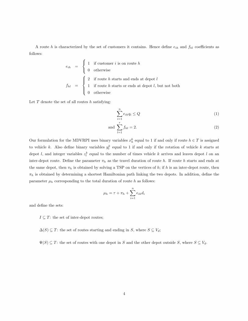
A route h is characterized by the set of customers it contains. Hence define eih and fhl coefficients as

follows:

eih =

1 if customer i is on route h

0 otherwise

fhl =

2 if route h starts and ends at depot l

1 if route h starts or ends at depot l, but not both

0 otherwise

Let T denote the set of all routes h satisfying:

n∑

i=1

eihqi ≤ Q (1)

and

r∑

l=1

fhl = 2. (2)

Our formulation for the MDVRPI uses binary variables xkh equal to 1 if and only if route h ∈ T is assigned

to vehicle k. Also define binary variables ykl equal to 1 if and only if the rotation of vehicle k starts at

depot l, and integer variables zkl equal to the number of times vehicle k arrives and leaves depot l on an

inter-depot route. Define the parameter πh as the travel duration of route h. If route h starts and ends at

the same depot, then πh is obtained by solving a TSP on the vertices of h; if h is an inter-depot route, then

πh is obtained by determining a shortest Hamiltonian path linking the two depots. In addition, define the

parameter µh corresponding to the total duration of route h as follows:

µh = τ + πh +

n∑

i=1

eihdi

and define the sets:

I ⊆ T : the set of inter-depot routes;

∆(S) ⊆ T : the set of routes starting and ending in S, where S ⊆ Vd;

Ψ(S) ⊆ T : the set of routes with one depot in S and the other depot outside S, where S ⊆ Vd.

4

The formulation is then:

Minimizem∑

k=1

|T |∑

h=1

πhxkh (3)

subject to

m∑

k=1

|T |∑

h=1

eihxkh = 1 i = 1, ..., n; (4)

r∑

l=1

ykl ≤ 1 k = 1, ..., m; (5)

∑

h∈I

fhlxkh − 2zk

l = 0 k = 1, ..., m; l = 1, ..., r; (6)

|T |∑

h=1

µhxkh ≤ D k = 1, ..., m; (7)

∑

h∈∆(S)

xkh ≤ |∆(S)|

∑

h∈Ψ(S)

xkh +

∑

l∈S

ykl

∀S ⊆ Vd; k = 1, ..., m; (8)

xkh ∈ {0, 1} ∀h, ∀k; (9)

ykl ∈ {0, 1} ∀k, ∀l; (10)

zkl integer ∀k, ∀l. (11)

Constraints (4) guarantee that each customer will be visited exactly once, while constraints (5) state that

at most one rotation will be assigned to every vehicle. Constraints (6) ensure that when a vehicle goes to

an intermediate depot, it also leaves it. Constraints (7) impose a limit on the total duration of a rotation.

Finally, (8) are subtour elimination constraints: given S ⊆ Vd, if at least one route of vehicle k belongs to

∆(S) (in which case the left-hand side of the inequality is positive), then there must exist at least one route

of that rotation in Ψ(S), or else one of the depots of S has to be the starting depot of that vehicle’s rotation

(since otherwise the right-hand side of the inequality is equal to zero).

3 Algorithm

Because the MDVRPI is an extension of the VRP and only small instances of the VRP can be solved exactly,

it is clear that one cannot expect to solve the MDVRPI with the above formulation. We have therefore opted

for the development of a tabu search (TS) heuristic. This choice is motivated by the success of TS for the

classical VRP and the MDVRP (see, for example, Cordeau et al. [8]).

5

In this section we will describe our algorithmic approach for the MDVRPI. It is based in part on the

adaptative memory principle proposed by Rochat and Taillard [27] where solutions are created by combining

elements of previously obtained solutions. Here single-depot and inter-depot routes will be combined. These

routes will be generated by means of a tabu search heuristic applied to three types of problems resulting from

the decomposition of the MDVRPI into an MDVRP, VRPs and inter-depot subproblems. In an inter-depot

problem, a set of minimal cost routes are generated on a network composed of customers and two depots,

where each route starts at one depot and ends at the other. From the solutions to the subproblems just

described, the underlying single-depot and inter-depot routes will be extracted and inserted in a solution

pool T . Next, an MDVRPI solution will be created by the execution of a set partitioning algorithm based

on the above formulation. Routes of T will therefore be selected so as to generate a set of feasible rotations

in which every customer is visited. Finally, a post-optimization phase will be performed in an attempt to

improve the solution.

This section successively describes the five components of our methodology: 1) the tabu search heuristic;

2) the procedure applied for the generation of a solution pool; 3) the route generation algorithm; 4) the set

partitioning algorithm, and 5) the post-optimization phase. This description is followed by a pseudo-code of

the algorithm.

3.1 Tabu search heuristic

Our tabu search heuristic is based on the TS heuristic proposed by Cordeau, Gendreau and Laporte [7] which

has proved highly effective for the solution of a wide range of classical vehicle routing problems, namely the

PVRP, the MDVRP as well as extensions of these problems containing time windows (Cordeau, Laporte and

Mercier [9]). We now recall the main features of this heuristic.

Neighbor solutions are obtained by removing a customer from its current route and reinserting it in

another route by means of the GENI procedure [13]. In the MDVRP, insertions can be made in a vehicle

associated with the same depot or with another depot. To implement tabu tenures for the VRP a set of

attributes (i, k) indicating that customer i is on the route of vehicle k is first defined. Whenever a customer

i is removed from route k, attribute (i, k) is declared tabu, and reinserting customer i in route k is forbidden

for a fixed number of iterations θ. The MDVRP works with attributes (i, k, l), meaning that customer i is on

the route of vehicle k from depot l. The tabu status of an attribute is revoked if the new solution is feasible

and of lesser cost than the best known solution having this attribute.

To broaden the search, infeasible intermediate solutions are allowed by associating a penalized objective

f(s) to each solution s. This function is a weighted sum of three terms: the actual solution cost c(s), the

violation q(s) of the capacity constraints, and the violation d(s) of the duration constraints. The global cost

6

function is then f(s) = c(s) + αq(s) + βd(s), where α and β are positive parameters dynamically updated

throughout the search, as will be explained in Section 3.3. If the solution is feasible the two functions c(s)

and f(s) coincide. This mechanism was first proposed by Gendreau, Hertz and Laporte [14] in the context

of the VRP. It allows the search to oscillate between feasible and infeasible solutions and enables the use

of simple neighborhoods which do not have to preserve feasibility. The parameter adjustment procedure

described in Section 3.3 leads to the examination of several good feasible solutions throughout the search.

A continuous diversification mechanism is applied to penalize frequent vertex moves. When a neighbor

solution s′ is obtained from the current solution s by adding attribute (i, k, l) and f(s′) > f(s), a penalty

g(s′) = γ√

nmr c(s)ρikl/λ is then added to f(s′). In g(s′), the factor γ is used to calibrate the intensity of

the diversification,√

nmr is a factor associated with problem size, λ is the current number of iterations, and

ρikl is a counter increased by one each time attribute (i, k, l) is added to the solution.

3.2 Generation of the solution pool

To create the solution pool T one must solve three types of subproblem: an MDVRP, a VRP, and an inter-

depot subproblem. The VRP is solved for each of the r depots, and the inter-depot subproblem is solved

for every pair of depots. In these two cases we only consider customers that could lead to the generation of

routes likely to belong to the solution of the original problem. The VRP associated with depot B contains

the following customers: 1) the ξn/r customers closest to B, where 0 < ξ ≤ 1 (in a planar problem this

defines a circle centered at B), and 2) the customers having B as their closest depot. There are two main

reasons for selecting customers defined by 2): first, there is a high probability that in an optimal solution a

customer will be served by its nearest depot; also this procedure includes some remote customers that might

not be frequently considered by 1) otherwise. The control parameter ξn/r limits the number of customers

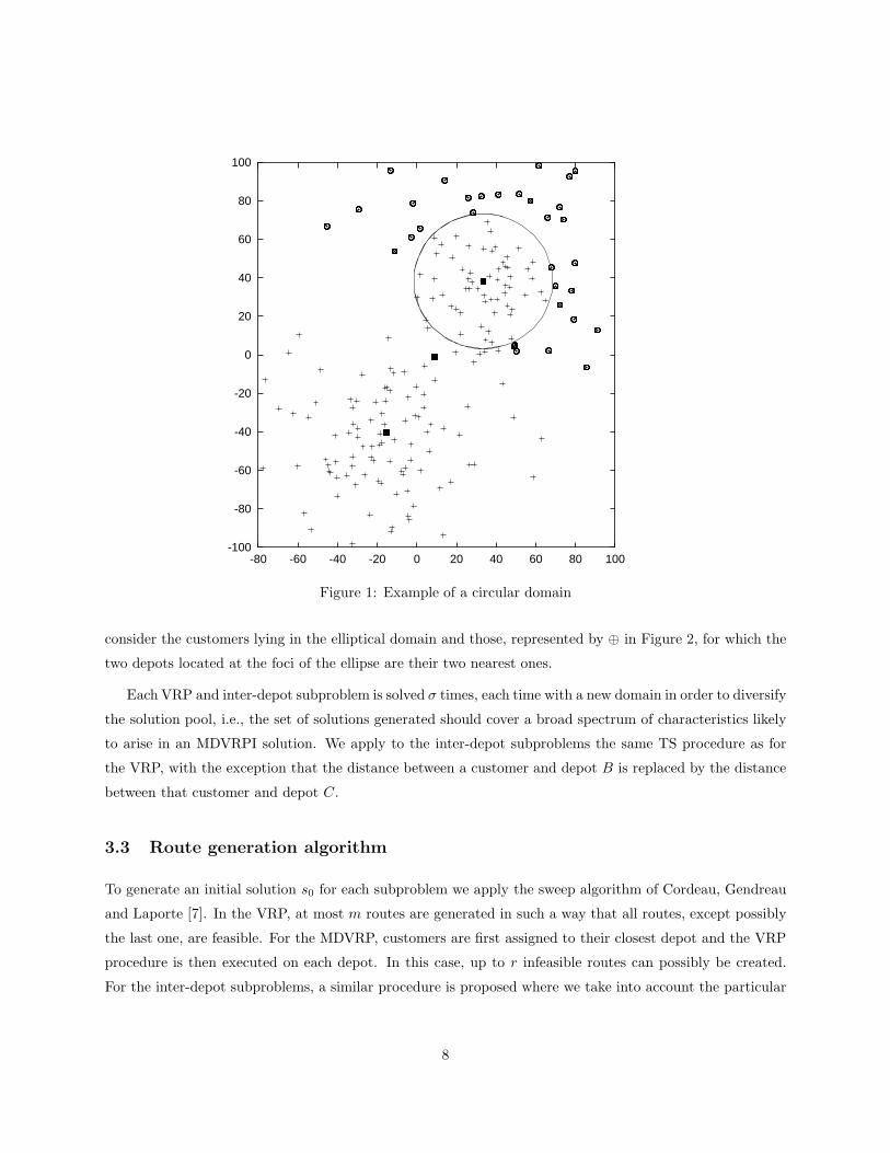
in each subproblem. Figure 1 shows the circular domain of a given subproblem. Customers lying outside

the domain but for which the considered depot is their closest one are represented by ⊕, while depots are

identified by �.

For the inter-depot subproblems, we propose a similar approach where, for a subproblem associated with

depots B and C, only customers sufficiently close to both B and C are considered for inclusion in the inter-

depot routes. In planar problems, a customer with coordinates (x, y) is selected if it satisfies the following

inequality:(

(x − a) cos(φ) + (y − b) sin(φ))2

ϕ21

+

(

(a − x) sin(φ) + (y − b) cos(φ))2

ϕ22

≤ 1.

This inequality defines the interior of an ellipse centered at (a, b), the midpoint of segment BC. The two

depots B and C will define the foci of the ellipse, while parameters ϕ1 and ϕ2 represent half the length of

the major and minor axis, respectively. The parameter φ defines the angle of rotation of the ellipse. We only

7

-100

-80

-60

-40

-20

0

20

40

60

80

100

-80 -60 -40 -20 0 20 40 60 80 100

Figure 1: Example of a circular domain

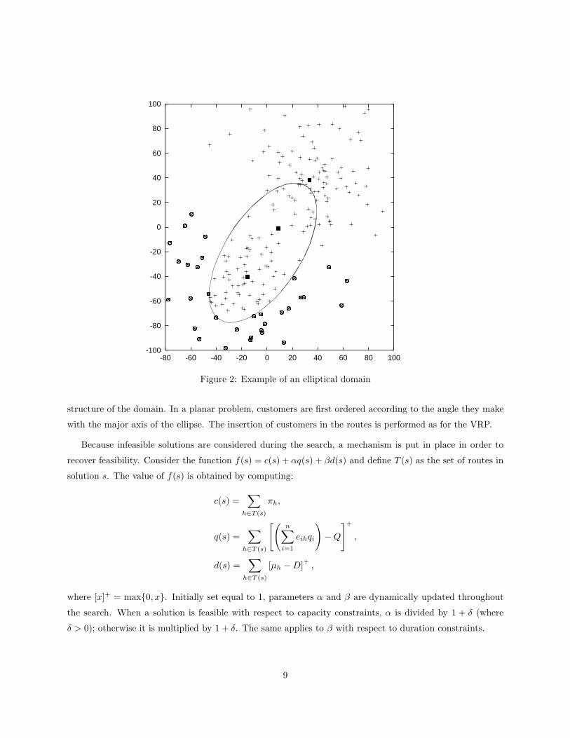
consider the customers lying in the elliptical domain and those, represented by ⊕ in Figure 2, for which the

two depots located at the foci of the ellipse are their two nearest ones.

Each VRP and inter-depot subproblem is solved σ times, each time with a new domain in order to diversify

the solution pool, i.e., the set of solutions generated should cover a broad spectrum of characteristics likely

to arise in an MDVRPI solution. We apply to the inter-depot subproblems the same TS procedure as for

the VRP, with the exception that the distance between a customer and depot B is replaced by the distance

between that customer and depot C.

3.3 Route generation algorithm

To generate an initial solution s0 for each subproblem we apply the sweep algorithm of Cordeau, Gendreau

and Laporte [7]. In the VRP, at most m routes are generated in such a way that all routes, except possibly

the last one, are feasible. For the MDVRP, customers are first assigned to their closest depot and the VRP

procedure is then executed on each depot. In this case, up to r infeasible routes can possibly be created.

For the inter-depot subproblems, a similar procedure is proposed where we take into account the particular

8

-100

-80

-60

-40

-20

0

20

40

60

80

100

-80 -60 -40 -20 0 20 40 60 80 100

Figure 2: Example of an elliptical domain

structure of the domain. In a planar problem, customers are first ordered according to the angle they make

with the major axis of the ellipse. The insertion of customers in the routes is performed as for the VRP.

Because infeasible solutions are considered during the search, a mechanism is put in place in order to

recover feasibility. Consider the function f(s) = c(s) + αq(s) + βd(s) and define T (s) as the set of routes in

solution s. The value of f(s) is obtained by computing:

c(s) =∑

h∈T (s)

πh,

q(s) =∑

h∈T (s)

[(

n∑

i=1

eihqi

)

− Q

]+

,

d(s) =∑

h∈T (s)

[µh − D]+

,

where [x]+ = max{0, x}. Initially set equal to 1, parameters α and β are dynamically updated throughout

the search. When a solution is feasible with respect to capacity constraints, α is divided by 1 + δ (where

δ > 0); otherwise it is multiplied by 1 + δ. The same applies to β with respect to duration constraints.

9

In order to control the cardinality of T , after solving a particular subproblem we only keep the routes

associated with a feasible solution whose cost does not exceed (1 + ǫ)c(s∗), where c(s∗) is the value of the

best solution identified, and ǫ is a positive parameter controlling the proportion of solutions that should be

kept.

3.4 Set partitioning algorithm

We now need to create a feasible solution to the MDVRPI from the pool of routes generated. We propose

a set partitioning algorithm based on the mathematical formulation described in Section 2. Because T does

not include all feasible routes it would be overly restrictive to impose that each customer should be visited

only once. We will therefore transform the set partitioning problem presented earlier into a set covering

problem. Also, to eliminate symmetric solutions, we impose that whenever i ≤ m, customer i be served by

vehicle k, where k ≤ i. Constraints (4) can now be transformed into:

min{i,m}∑

k=1

|T |∑

h=1

eihxkh ≥ 1 i = 1, ..., n.

We ensure that each customer is covered only once in the final solution. The criterion applied to remove a

customer is the largest saving obtained with the GENI heuristic.

Finally, we tighten the subtour elimination constraints by making use of the information on the duration

of the routes in ∆(S) and on the maximal duration of a rotation. We first define the set ∆′(S) as follows:

1. set ∆′(S) := ∅;

2. while∑

h∈∆′(S)

µh < D, set ∆′(S) := ∆′(S) ∪ arg minh∈∆(S)\∆′(S)

{µh},

and we rewrite constraints (8) as

∑

h∈∆(S)

xkh ≤ |∆′(S)|

∑

h∈Ψ(S)

xkh +

∑

l∈S

ykl

∀S ⊆ Vd; k = 1, ..., m.

The idea is to use as a bound the maximal number of routes in ∆(S) that can be assigned to a vehicle

without violating the duration constraint of a rotation. The effect of this is to increase the value of the lower

bound by the linear programming relaxation of the set partitioning problem.

3.5 Post-optimization

In the post-optimization phase, we attempt to improve the solution composed of the routes of the set T ′

defined as the routes from the original pool T selected by the set partitioning algorithm. We use the tabu

10

search heuristic previously described with three slight modifications. First, we now consider the attributes

(i, h, k) indicating that customer i is on route h in the rotation of vehicle k. Next, the component d(s) of

f(s) is modified to take into account the assigment of more than one route to a vehicle. The new definition

is

d(s) =

m∑

k=1

[(

∑

h∈T ′

µhxkh

)

− D

]+

.

Finally, the factor used in the diversification procedure to compensate for problem size when evaluating g(s′)

is now√

n|T ′|, the square root of the number of possible attributes.

The tabu search procedure is first applied to the solution corresponding to the set T ′ of routes. Rotations

containing empty routes in the best solution are identified and empty routes are eliminated. Note that

removing inter-depot routes from a rotation may lead to an infeasible solution due, for example, to the

creation of subtours, or to violations of the constraints stating that a rotation has to start and end at the

same depot. We have therefore devised an enumerative procedure to restore feasibility. The first step consists

of modifying the remaining routes of the rotation by eliminating the edges incident to the depots. All feasible

sequences of routes and depots are enumerated and the least cost rotation is identified. Obviously, the first

and last depot of the sequence must be identical. Tabu search is then reapplied to the feasible solution and

the post-optimization process is repeated until no empty route is generated by the tabu search.

3.6 Pseudo-codes of the algorithm

Our notation is summarized in Tables 1 to 4 and the main steps of the algorithm are described in the

following pseudo-codes. The MDVRPI heuristic performs, in sequence, Algorithm 1, the set partitioning

algorithm (Cplex based) and Algorithm 2.

4 Computational results

This section presents a sensitivity analysis of the parameters as well as computational results. We first

describe how the benchmark instances were generated. The sensitivity analyses follow. Finally, numerical

results are presented on the randomly generated instances as well as MDVRP instances proposed by Cordeau,

Gendreau and Laporte [7], adapted to the context of the MDVRPI.

4.1 MDVRPI : general case

The aim of the MDVRPI is the creation of at most m least cost feasible rotations such that each customer

is visited once by a route belonging to the rotation of one of the m vehicles. Preliminary tests conducted on

11

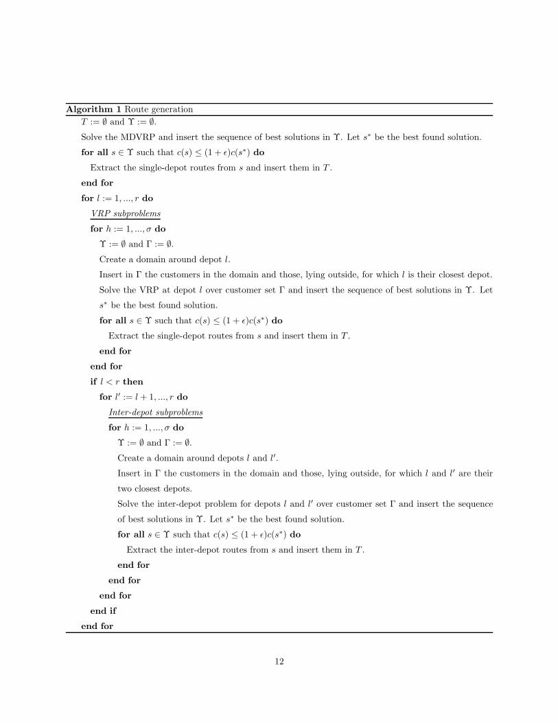
Algorithm 1 Route generation

T := ∅ and Υ := ∅.Solve the MDVRP and insert the sequence of best solutions in Υ. Let s∗ be the best found solution.

for all s ∈ Υ such that c(s) ≤ (1 + ǫ)c(s∗) do

Extract the single-depot routes from s and insert them in T .

end for

for l := 1, ..., r do

VRP subproblems

for h := 1, ..., σ do

Υ := ∅ and Γ := ∅.Create a domain around depot l.

Insert in Γ the customers in the domain and those, lying outside, for which l is their closest depot.

Solve the VRP at depot l over customer set Γ and insert the sequence of best solutions in Υ. Let

s∗ be the best found solution.

for all s ∈ Υ such that c(s) ≤ (1 + ǫ)c(s∗) do

Extract the single-depot routes from s and insert them in T .

end for

end for

if l < r then

for l′ := l + 1, ..., r do

Inter-depot subproblems

for h := 1, ..., σ do

Υ := ∅ and Γ := ∅.Create a domain around depots l and l′.

Insert in Γ the customers in the domain and those, lying outside, for which l and l′ are their

two closest depots.

Solve the inter-depot problem for depots l and l′ over customer set Γ and insert the sequence

of best solutions in Υ. Let s∗ be the best found solution.

for all s ∈ Υ such that c(s) ≤ (1 + ǫ)c(s∗) do

Extract the inter-depot routes from s and insert them in T .

end for

end for

end for

end if

end for

12

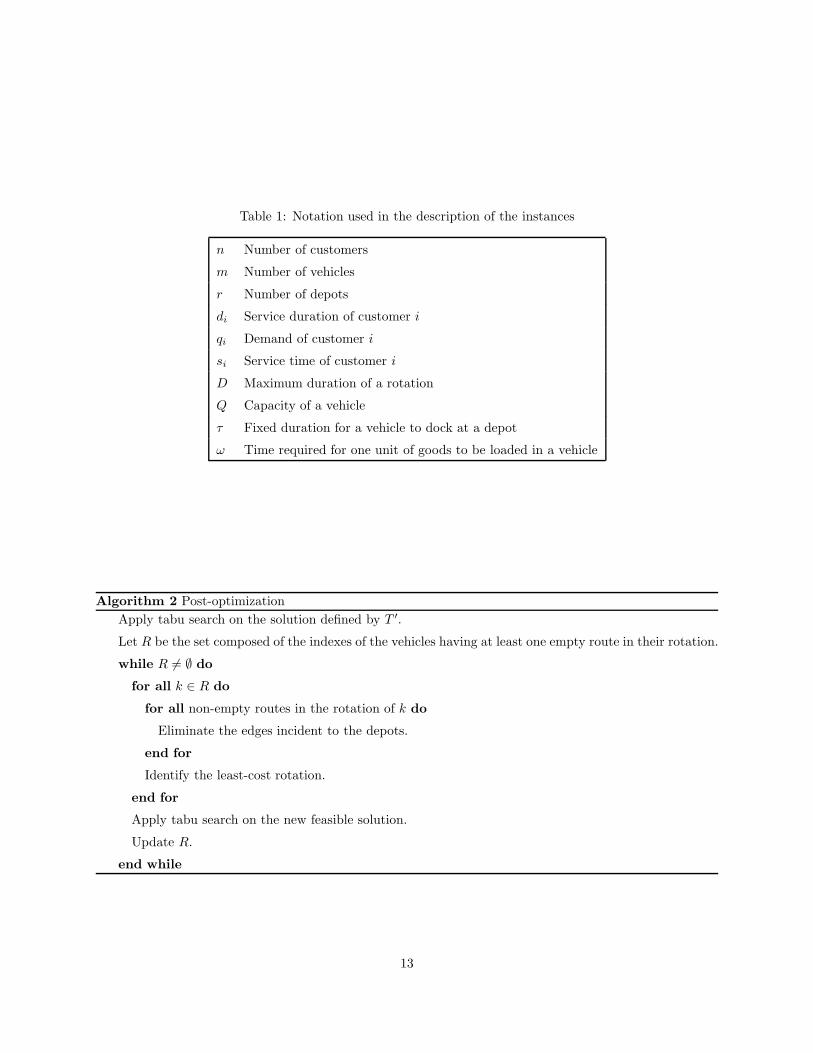
Table 1: Notation used in the description of the instances

n Number of customers

m Number of vehicles

r Number of depots

di Service duration of customer i

qi Demand of customer i

si Service time of customer i

D Maximum duration of a rotation

Q Capacity of a vehicle

τ Fixed duration for a vehicle to dock at a depot

ω Time required for one unit of goods to be loaded in a vehicle

Algorithm 2 Post-optimization

Apply tabu search on the solution defined by T ′.

Let R be the set composed of the indexes of the vehicles having at least one empty route in their rotation.

while R 6= ∅ do

for all k ∈ R do

for all non-empty routes in the rotation of k do

Eliminate the edges incident to the depots.

end for

Identify the least-cost rotation.

end for

Apply tabu search on the new feasible solution.

Update R.

end while

13

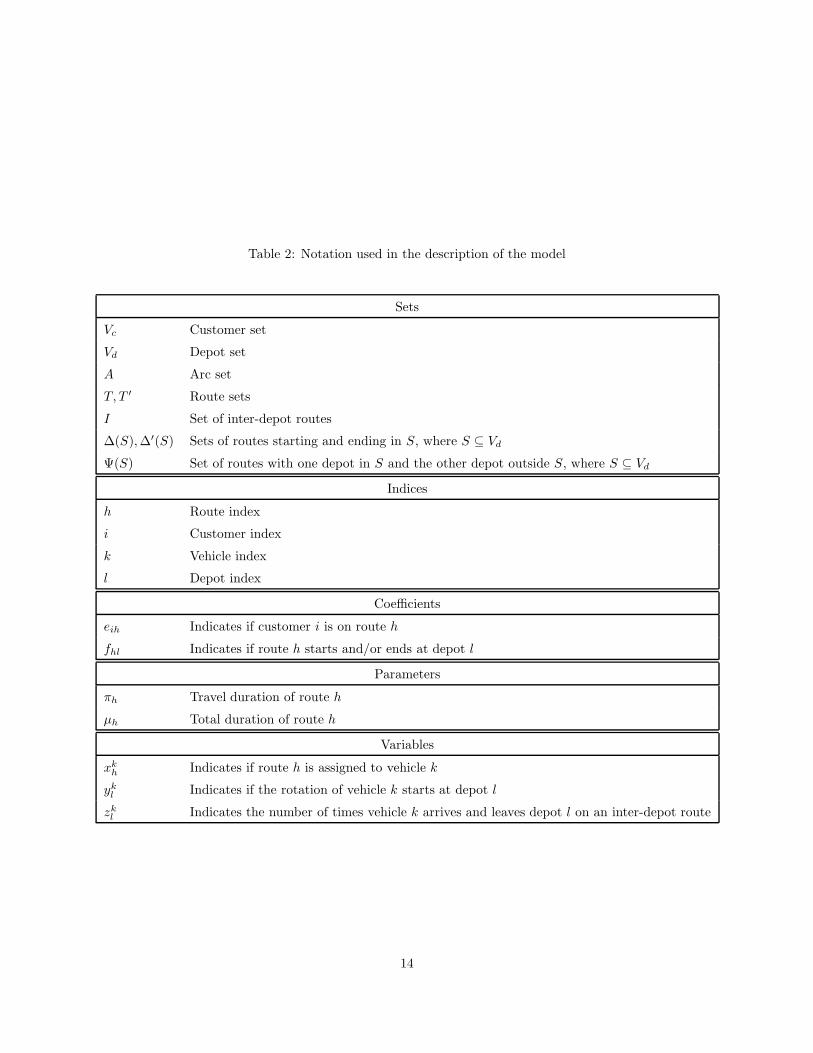
Table 2: Notation used in the description of the model

Sets

Vc Customer set

Vd Depot set

A Arc set

T, T ′ Route sets

I Set of inter-depot routes

∆(S), ∆′(S) Sets of routes starting and ending in S, where S ⊆ Vd

Ψ(S) Set of routes with one depot in S and the other depot outside S, where S ⊆ Vd

Indices

h Route index

i Customer index

k Vehicle index

l Depot index

Coefficients

eih Indicates if customer i is on route h

fhl Indicates if route h starts and/or ends at depot l

Parameters

πh Travel duration of route h

µh Total duration of route h

Variables

xkh Indicates if route h is assigned to vehicle k

ykl Indicates if the rotation of vehicle k starts at depot l

zkl Indicates the number of times vehicle k arrives and leaves depot l on an inter-depot route

14

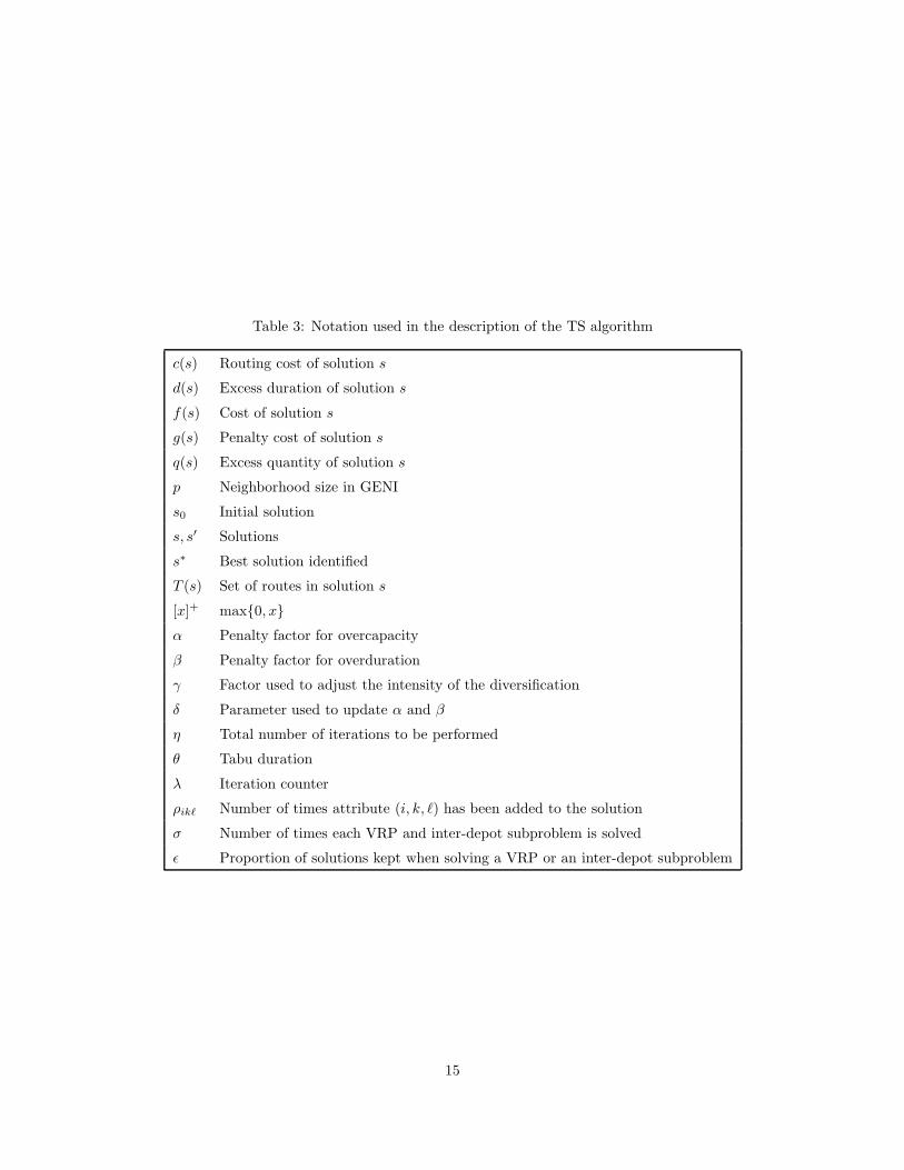
Table 3: Notation used in the description of the TS algorithm

c(s) Routing cost of solution s

d(s) Excess duration of solution s

f(s) Cost of solution s

g(s) Penalty cost of solution s

q(s) Excess quantity of solution s

p Neighborhood size in GENI

s0 Initial solution

s, s′ Solutions

s∗ Best solution identified

T (s) Set of routes in solution s

[x]+ max{0, x}α Penalty factor for overcapacity

β Penalty factor for overduration

γ Factor used to adjust the intensity of the diversification

δ Parameter used to update α and β

η Total number of iterations to be performed

θ Tabu duration

λ Iteration counter

ρikℓ Number of times attribute (i, k, ℓ) has been added to the solution

σ Number of times each VRP and inter-depot subproblem is solved

ǫ Proportion of solutions kept when solving a VRP or an inter-depot subproblem

15

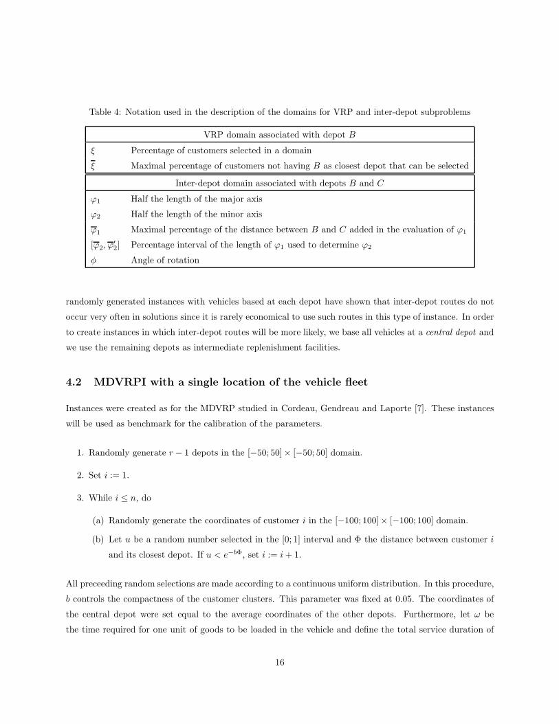
Table 4: Notation used in the description of the domains for VRP and inter-depot subproblems

VRP domain associated with depot B

ξ Percentage of customers selected in a domain

ξ Maximal percentage of customers not having B as closest depot that can be selected

Inter-depot domain associated with depots B and C

ϕ1 Half the length of the major axis

ϕ2 Half the length of the minor axis

ϕ1 Maximal percentage of the distance between B and C added in the evaluation of ϕ1

[ϕ2, ϕ′2] Percentage interval of the length of ϕ1 used to determine ϕ2

φ Angle of rotation

randomly generated instances with vehicles based at each depot have shown that inter-depot routes do not

occur very often in solutions since it is rarely economical to use such routes in this type of instance. In order

to create instances in which inter-depot routes will be more likely, we base all vehicles at a central depot and

we use the remaining depots as intermediate replenishment facilities.

4.2 MDVRPI with a single location of the vehicle fleet

Instances were created as for the MDVRP studied in Cordeau, Gendreau and Laporte [7]. These instances

will be used as benchmark for the calibration of the parameters.

1. Randomly generate r − 1 depots in the [−50; 50]× [−50; 50] domain.

2. Set i := 1.

3. While i ≤ n, do

(a) Randomly generate the coordinates of customer i in the [−100; 100]× [−100; 100] domain.

(b) Let u be a random number selected in the [0; 1] interval and Φ the distance between customer i

and its closest depot. If u < e−bΦ, set i := i + 1.

All preceeding random selections are made according to a continuous uniform distribution. In this procedure,

b controls the compactness of the customer clusters. This parameter was fixed at 0.05. The coordinates of

the central depot were set equal to the average coordinates of the other depots. Furthermore, let ω be

the time required for one unit of goods to be loaded in the vehicle and define the total service duration of

16

customer i as di = si + ωqi where the service time si and the demand qi are selected in the [1; 25] interval

according to a discrete uniform distribution. We set τ = 15 and ω = 0.25. Finally, D and Q were determined

experimentally in order to guarantee the feasibility of the instance. Table 1 summarizes the characteristics

of the instances on which the algorithm was tested.

Table 5: Characteristics of MDVRPI instances

Instance r n m D Q

a1 3 48 6 550 60

b1 3 96 4 1200 210

c1 3 192 5 1850 360

d1 4 48 5 600 80

e1 4 96 5 1300 230

f1 4 192 4 2000 380

g1 5 72 5 750 80

h1 5 144 4 1550 230

i1 5 216 4 2350 380

j1 6 72 4 800 100

k1 6 144 4 1650 250

l1 6 216 4 2500 400

4.3 Sensitivity analyses

Several parameters must be calibrated in order to obtain a good balance between solution quality and

computational time.

4.3.1 Parameters δ, γ, θ, p and η

The tabu search heuristic requires the tuning of the five following parameters : 1) a parameter δ controlling

the dynamic update of α and β; 2) a parameter γ controlling the diversification intensity; 3) θ, the number

of iterations during which an attribute is considered tabu; 4) p, the neighborhood size in GENI; 5) η, the

total number of iterations to be performed by the algorithm.

The best values of these parameters were extensively studied by Cordeau, Gendreau and Laporte [7] and

by Cordeau, Laporte and Mercier [9]. A conclusion of these authors is that the best parameter values are

remarkably stable over a wide range of problems such as the VRP, the MDVRP, the PVRP and variants of

these problems with time windows. Setting δ = 0.5, γ = 0.015, θ = [7.5 log10 n] (where [x] represents the

integer closest to x), and p = 3 is recommended. Because our problem has a structure similar to that of the

17

VRP and the MDVRP we have used the same settings for δ, γ, θ and p. The number η of iterations is left

to the user.

4.3.2 Parameters ξ, ξ, ϕ1, ϕ1, ϕ2, (ϕ2, ϕ′2), σ and ǫ

Having fixed most of the tabu search parameters, we now discuss those defining the VRP and inter-depot

domains. The parameter ξ shaping the boundary of the VRPs is selected, as mentioned earlier, in the

]0; 1] interval according to a continuous uniform distribution. However, for a VRP associated with depot

B, since customers for which the depot is their closest one are considered, the value of ξ is chosen so that

up to ξ percent of the customers closest to B, but not having B as their closest depot, can be selected.

The parameters ϕ1 and ϕ2 defining the region in the inter-depot subproblems are determined as follows.

Consider the problem associated with depots B and C and let cBC be the distance between these two

depots. Since in a planar instance ϕ1 corresponds to half the length of the major axis going through the

depots, at least half the distance between the two depots will be assigned to it. Also, we add a random

value selected in the [0; ϕ1 cBC ] interval, where 0 ≤ ϕ1 ≤ 1, so that ϕ1 cBC represent a certain percentage

of cBC . Consequently ϕ1 := cBC/2 + uϕ1 cBC , where u ∈ [0; 1] is a randomly chosen number according to

a continuous uniform distribution. Finally, once ϕ1 is set, the length of the half-axis ϕ2 will be randomly

selected in the [ϕ2ϕ1; ϕ′2ϕ1] interval with 0 ≤ ϕ2 < ϕ′

2 ≤ 1 which defines ϕ2 as a certain percentage of

ϕ1. Therefore, ϕ2 := uϕ1, where u ∈ [ϕ2; ϕ′2]. The values of ϕ1, ϕ2 and ϕ′

2 will be discussed next. The

parameters were analyzed jointly since tight relations can be expected among them.

To determine the value assignment to the parameters just described, a preliminary version of the algorithm

was tested on the instances described in Section 4.2. The parameters σ and ǫ, defining respectively the number

of times each VRP or inter-depot subproblem is solved, and the proportion of solutions to keep when solving

a subproblem, were set equal to 10 and 0.01. These values were selected so as to create a diversity of solutions

possessing characteristics that might arise in good MDVRPI solutions. The value of η was set equal to 7500

for the VRP and inter-depot subproblems, and to 15,000 for the MDVRP. In the post-optimization phase,

preliminary tests have shown that recursive calls to the tabu search heuristic require a decreasing number of

iterations to adequately explore the solution space. That is why η was fixed at 45,000 in the first call and

at 30,000 in the subsequent calls.

Tests have shown that allowing the selection of large inter-depot domains leads, on average, to better

solutions. Larger domains generate larger clusters of customers, resulting in the creation of superior route

structures. However, because more customers are considered each time a subproblem is solved, more routes

are generated and the size of T increases. Two combinations of parameters stand out: ξ = 0.2, ϕ1 = 1,

(ϕ2, ϕ′2) = (0.5, 1) and ξ = 0.6, ϕ1 = 1, (ϕ2, ϕ

′2) = (0.25, 0.5). The first parameter combination generates

better results on average but requires more computational time on large size instances. The second one

18

produces slightly worse results on average but yields more stable computational times. Further tests have

shown that the second parameter combination, combined with ǫ = 0.01 and σ = 12 yields the best results.

4.4 Results on benchmark instances

We now present the results of tests conducted on the 12 MDVRPI instances of Table 1 and on a set of

instances derived from the MDVRP instances of Cordeau, Gendreau and Laporte [7]. These instances and

the best known solutions are available at http://www.hec.ca/chairedistributique/data/. They vary in

size from n = 48 to n = 288, which is consistent with the size of the benchmark instances commonly used for

the MDVRP (see Cordeau, Gendreau and Laporte [7]). The algorithm was coded in C and the set covering

problem was solved with CPLEX 7.1. Tests were run on a Prosys, 2 GHz computer. All computations were

performed in double precision arithmetic and the final results are reported with two significant digits after

the decimal point.

4.4.1 Results on randomly generated instances

The algorithm was executed with the following parameter values: ξ = 0.6, ϕ1 = 1, (ϕ2, ϕ′2) = (0.25, 0.5),

σ = 12, ǫ = 0.01. The number of iterations η is set equal to 15,000 in the solution of the MDVRP, and

to 5000 in the VRP and inter-depot subproblems since tests have shown that a sufficent exploration of the

solution space is performed with these values. Furthermore, the first two executions of the tabu search

heuristic in the post-optimization phase seemed to be the most crucial since it is during those calls that the

structure of the solution is mostly modified. We have therefore set η = 35,000 in the first call, 25,000 in the

second one and 15,000 in the following calls. The heuristic was executed ten times on each of the randomly

generated instances. Table 2 provides results. The column headings are defined as follows:

– c(s∗), the average value of the solutions over the ten runs;

– c(sb), the value of the best solution identified throughout the sensitivity analyses;

– %, the gap in percentage between the average value of the solutions and the best known solution;

– %b, the percentage gap between c(sb) and the best solution found among the ten solutions generated;

– %w, the percentage gap between c(sb) and the worst solution identified among the ten solutions ob-

tained;

– |T |, the average cardinality of the set T ;

– tgen, the average time, in minutes, spent on route generation;

– tspa, the average time required by the set partitioning algorithm;

– tpo, the average time of the post-optimization phase;

– ttot, the average total computational time.

19

Table 6: Solutions obtained on MDVRPI instances

Instance c(s∗) c(sb) % %b %w |T | tgen tspa tpo ttot

a1 1211.28 1179.79 2.67 2.00 3.10 317.90 2.44 1.40 0.74 4.58

b1 1232.67 1217.07 1.28 0.00 2.43 555.30 6.36 0.23 2.58 9.17

c1 1893.01 1886.15 0.36 0.11 0.66 1340.50 23.08 3.04 10.10 36.22

d1 1076.31 1059.43 1.59 0.00 3.48 350.90 2.57 4.93 1.05 8.55

e1 1311.60 1309.12 0.19 0.00 1.89 469.10 7.46 0.49 5.57 13.52

f1 1601.54 1576.33 1.60 1.01 2.18 1107.50 21.18 4.27 15.95 41.41

g1 1202.00 1181.13 1.77 0.83 2.79 641.40 5.01 48.33 1.88 55.22

h1 1598.51 1547.25 3.31 1.26 5.83 866.30 13.97 8.60 9.49 32.07

i1 1976.11 1927.99 2.50 0.92 3.27 1334.100 25.81 6.09 19.11 51.01

j1 1161.77 1120.65 3.67 2.12 6.56 916.10 7.39 48.99 2.53 58.90

k1 1618.45 1586.92 1.99 0.00 3.79 1568.50 17.37 39.55 7.70 64.61

l1 1917.08 1884.92 1.71 0.68 3.22 2002.80 34.20 48.38 21.69 104.27

Average 1483.36 1456.40 1.89 0.74 3.27 955.87 13.90 17.86 8.20 39.96

The average is computed and presented in bold at the end of the corresponding column.

We observe that the average percentage gap between the average and best solution values for each instance

is 1.89% and the average percentage gap between the overall best and worst values over the ten runs on each

instance is 3.27%, which is reasonable given the many random components of the algorithm. More stability

can be reached through the use of higher values for σ or ǫ and at the expense of longer computational times.

Computational times are closely related to instance size and to the tightness of constraints (1) and (7). For

a given instance, the variability in computational time is mostly explained by the time spent in the solution

of the set covering problem.

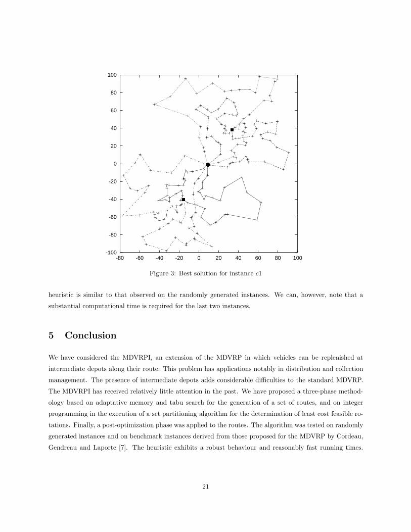
Figure 3 depicts the best solution obtained for instance c1. The central depot is identified by • and

the other depots by �. Every vehicle route is represented by a different line type. We can distinguish four

rotations, each composed of two inter-depot routes.

4.4.2 Results on the Cordeau, Gendreau and Laporte instances

Ten new instances were generated from those proposed by Cordeau, Gendreau and Laporte [7] for the

MDVRP. These instances contain between 48 and 288 customers as well as four or six depots. In order to

adapt the instances to the MDVRPI, a central depot was added at the centroıd of the other depots. The

resulting instances contain either five or seven depots. The values of D and Q were determined experimentally

to guarantee feasibility. Table 3 summarizes the main characteristics of the modified instances and Table 4

presents the results. Again, the algorithm was executed ten times on each instance. The behaviour of the

20

-100

-80

-60

-40

-20

0

20

40

60

80

100

-80 -60 -40 -20 0 20 40 60 80 100

Figure 3: Best solution for instance c1

heuristic is similar to that observed on the randomly generated instances. We can, however, note that a

substantial computational time is required for the last two instances.

5 Conclusion

We have considered the MDVRPI, an extension of the MDVRP in which vehicles can be replenished at

intermediate depots along their route. This problem has applications notably in distribution and collection

management. The presence of intermediate depots adds considerable difficulties to the standard MDVRP.

The MDVRPI has received relatively little attention in the past. We have proposed a three-phase method-

ology based on adaptative memory and tabu search for the generation of a set of routes, and on integer

programming in the execution of a set partitioning algorithm for the determination of least cost feasible ro-

tations. Finally, a post-optimization phase was applied to the routes. The algorithm was tested on randomly

generated instances and on benchmark instances derived from those proposed for the MDVRP by Cordeau,

Gendreau and Laporte [7]. The heuristic exhibits a robust behaviour and reasonably fast running times.

21

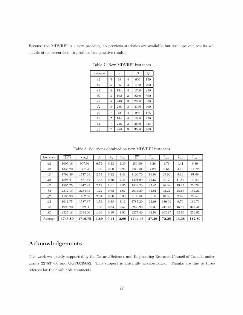
Because the MDVRPI is a new problem, no previous statistics are available but we hope our results will

enable other researchers to produce comparative results.

Table 7: New MDVRPI instances

Instance r n m D Q

a2 5 48 4 600 150

b2 5 96 4 1150 200

c2 5 144 4 1700 250

d2 5 192 3 2250 300

e2 5 240 3 2800 350

f2 5 288 3 3350 400

g2 7 72 4 950 175

h2 7 144 4 1800 250

i2 7 216 3 2650 325

j2 7 288 3 3500 400

Table 8: Solutions obtained on new MDVRPI instances

Instance c(s∗) c(sb) % %b %w |T | tgen tspa tpo ttot

a2 1005.16 997.94 0.72 0.23 1.30 259.90 3.26 1.71 1.41 6.39

b2 1333.20 1307.28 1.98 0.00 2.95 683.10 7.89 2.64 4.19 14.72

c2 1792.46 1747.61 2.57 0.22 4.41 1100.70 16.98 35.60 9.10 61.68

d2 1898.21 1871.42 1.43 0.30 2.41 1494.90 22.62 6.12 11.80 40.54

e2 1995.75 1942.85 2.72 1.61 3.35 1539.20 27.45 26.38 19.95 73.78

f2 2312.15 2284.35 1.22 0.62 1.67 2637.20 44.81 92.22 25.19 162.22

g2 1185.93 1162.58 2.01 0.00 5.36 714.10 8.10 18.53 2.89 29.51

h2 1611.75 1587.37 1.54 0.38 3.11 1787.20 21.08 130.01 9.70 160.79

i2 1998.20 1972.00 1.33 0.34 2.51 3950.90 58.39 247.13 16.89 322.41

j2 2325.18 2294.06 1.36 0.39 1.92 3277.40 61.99 162.17 32.70 256.85

Average 1745.80 1716.75 1.69 0.41 2.90 1744.46 27.26 72.25 13.38 112.89

Acknowledgements

This work was partly supported by the Natural Sciences and Engineering Research Council of Canada under

grants 227837-00 and OGP0039682. This support is gratefully acknowledged. Thanks are due to three

referees for their valuable comments.

22

References

[1] E. Angelelli and M. G. Speranza. The application of a vehicle routing model to a waste-collection

problem: two case studies. Journal of the Operational Research Society, 53:944–952, 2002.

[2] E. Angelelli and M. G. Speranza. The periodic vehicle routing problem with intermediate facilities.

European Journal of Operational Research, 137:233–247, 2002.

[3] J. C. S. Brandao and A. Mercer. A tabu search algorithm for the multi-trip vehicle routing and scheduling

problem. European Journal of Operational Research, 100:180–191, 1997.

[4] J. C. S. Brandao and A. Mercer. The multi-trip vehicle routing problem. Journal of the Operational

Research Society, 49:799–805, 1998.

[5] F. Cano Sevilla and C. Simon de Blas. Vehicle routing problem with time windows and intermediate

facilities. S.E.I.O.’03 Edicions de la Universitat de Lleida, pages 3088–3096, 2003.

[6] I-M. Chao, B. L. Golden, and E. A. Wasil. A new heuristic for the multi-depot vehicle routing prob-

lem that improves upon best-known solutions. American Journal of Mathematical and Management

Sciences, 13:371–406, 1993.

[7] J.-F. Cordeau, M. Gendreau, and G. Laporte. A tabu search heuristic for periodic and multi-depot

vehicle routing problems. Networks, 30:105–119, 1997.

[8] J.-F. Cordeau, M. Gendreau, G. Laporte, J.-Y. Potvin, and F. Semet. A guide to vehicle routing

heuristics. Journal of the Operational Research Society, 53:512–522, 2002.

[9] J.-F. Cordeau, G. Laporte, and A. Mercier. A unified tabu search heuristic for vehicle routing problems

with time windows. Journal of the Operational Research Society, 52:928–936, 2001.

[10] G. Dueck. New optimization heuristics: The great deluge algorithm and the record-to-record travel.

Journal of Computational Physics, 104:86–92, 1993.

[11] K. Fagerholt. Designing optimal routes in a liner shipping problem. Maritime Policy & Management,

31:259–268, 2004.

[12] B. Fleischmann. The vehicle routing problem with multiple use of vehicles. Working paper, Fachbereich

Wirtschaftswissenschaften, Universitat Hamburg, 1990.

[13] M. Gendreau, A. Hertz, and G. Laporte. New insertion and postoptimization procedures for the traveling

salesman problem. Operations Research, 40:1086–1094, 1992.

23

[14] M. Gendreau, A. Hertz, and G. Laporte. A tabu search heuristic for the vehicle routing problem.

Management Science, 40:1276–1290, 1994.

[15] M. Gendreau, G. Laporte, and J.-Y. Potvin. Metaheuristics for the capacitated vehicle routing problem.

In P. Toth and D. Vigo, editors, The Vehicle Routing Problem, pages 129–154. SIAM Monographs on

Discrete Mathematics and Applications, Philadelphia, 2002.

[16] B. E. Gillett and J. G. Johnson. Multi-terminal vehicle-dispatch algorithm. Omega, 4:711–718, 1976.

[17] B. L. Golden, T. L. Magnanti, and H. Q. Nguyen. Implementing vehicle routing algorithms. Networks,

7:113–148, 1977.

[18] W. C. Jordan. Truck backhauling on networks with many terminals. Transportation Research, 21B:183–

193, 1987.

[19] W. C. Jordan and L. D. Burns. Truck backhauling on two terminal networks. Transportation Research,

18B:487–503, 1984.

[20] G. Laporte, Y. Nobert, and D. Arpin. Optimal solutions to capacitated multidepot vehicle routing

problems. Congressus Numerantium, 44:283–292, 1984.

[21] G. Laporte, Y. Nobert, and S. Taillefer. Solving a family of multi-depot vehicle routing and location-

routing problems. Transportation Science, 22:161–172, 1988.

[22] G. Laporte and F. Semet. Classical heuristics for the capacitated vehicle routing problem. In P. Toth

and D. Vigo, editors, The Vehicle Routing Problem, pages 109–128. SIAM Monographs on Discrete

Mathematics and Applications, Philadelphia, 2002.

[23] S. Lin. Computer solutions of the traveling salesman problem. Bell System Technical Journal, 44:2245–

2269, 1965.

[24] O. M. Raft. A modular algorithm for an extended vehicle scheduling problem. European Journal of

Operational Research, 11:67–76, 1982.

[25] J. Renaud, G. Laporte, and F. F. Boctor. An improved petal heuristic for the vehicle routing problem.

Journal of the Operational Research Society, 47:329–336, 1996.

[26] J. Renaud, G. Laporte, and F. F. Boctor. A tabu search heuristic for the multi-depot vehicle routing

problem. Computers & Operations Research, 23:229–235, 1996.

[27] Y. Rochat and E. D. Taillard. Probabilistic diversification and intensification in local search for vehicle

routing. Journal of Heuristics, 1:147–167, 1995.

24

[28] Suprayogi, H. Yamato, and Iskendar. Ship routing design for the oily liquid waste collection. Journal

of the Society of Naval Architects of Japan, 190:325–335, 2001.

[29] E. D. Taillard, G. Laporte, and M. Gendreau. Vehicle routeing with multiple use of vehicles. Journal

of the Operational Research Society, 47:1065–1070, 1996.

[30] F. A. Tillman. The multiple terminal delivery problem with probabilistic demands. Transportation

Science, 3:192–204, 1969.

[31] F. A. Tillman and T. M. Cain. An upperbound algorithm for the single and multiple terminal delivery

problem. Management Science, 18:664–682, 1972.

[32] F. A. Tillman and R. W. Hering. A study of look-ahead procedure for solving the multiterminal delivery

problem. Transportation Research, 5:225–229, 1971.

[33] A. Wren and A. Holliday. Computer scheduling of vehicles from one or more depots to a number of

delivery points. Operational Research Quarterly, 23:333–344, 1972.

[34] Q.-H. Zhao, S.-Y. Wang, K-K Lai, and G.-P. Xia. A vehicle routing problem with multiple use of

vehicles. Advanced Modeling and Optimization, 4:21–40, 2002.

25