The Multi-Probe Method

DES-Y1 results on behalf of the Dark Energy Survey Collaboration

Elisabeth KrauseUniversity of Arizona

Berkeley Weak Lensing Workshop, January 2019

The Power of Combining Probes

• Best constraints obtained by combining cosmological probes

- independent probes: multiply likelihoods

• Combining LSS probes (from same survey) requires more complicated analyses

- clustering, clusters and WL probe same underlying density field, are correlated

- correlated systematic effects

→ requires joint analysisOlivier Doré AAS, WFIRST Science, Kissimmee, January 5th 2016

The Observational Foundations of Dark Energy

• Weak-Lensing not presented is also complementary.2

SNe luminosity !distance measurement (Nobel 2011)

CMB angular diameter!distance measurement! and perturbations

BAO angular !diameter distance!measurement!

Combination

Matter Density

Cosmological !Constant, !i.e. Dark Energy

Joint Analysis Ingredients

Likelihood Function Model Data Vector

Joint Covariance

number counts: Poisson

2PCF: ~ Gaussian (?)

improvements needed for stage IV surveys

consistent modeling of all observables

including all cosmology + nuisance parameters

large and complicated,non-(block) diagonal matrixuse template + regularization (?)

External DataSimulations

Science Caseparameters of interest which science?

large data vector which probes + scales?

Priors

Nuisance Parameters

systematic effects

parameterize + prioritize!|n| � |⇡|

validate

p(⇡|d̂) / p(⇡)

ZL⇣d̂|d(⇡,n), C

⌘p(n) dnn

Cosmology Priors

“Precision” Cosmology

precision BIG SURVEYS

“Precision” Cosmology

precision BIG SURVEYS

“Precision” Cosmology

precision

accu

racy

BIG SURVEYS

COMPLEX ANALYSES

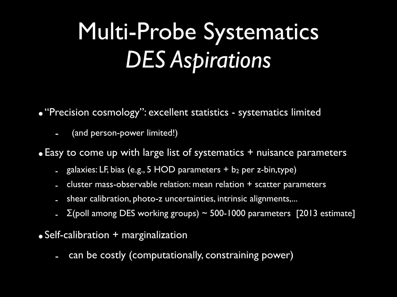
Multi-Probe SystematicsDES Aspirations

•“Precision cosmology”: excellent statistics - systematics limited

- (and person-power limited!)

•Easy to come up with large list of systematics + nuisance parameters

- galaxies: LF, bias (e.g., 5 HOD parameters + b2 per z-bin,type)

- cluster mass-observable relation: mean relation + scatter parameters

- shear calibration, photo-z uncertainties, intrinsic alignments,...

- Σ(poll among DES working groups) ~ 500-1000 parameters [2013 estimate]

•Self-calibration + marginalization

- can be costly (computationally, constraining power)

DES Year 1 Cosmology Analysis

galaxies x galaxies: angular clustering

lensing x lensing: cosmic sheargalaxies x lensing:

galaxy-galaxy lensing

θ θθ

Chang(+DES) 2018Elvin-Poole(+DES) 2018

baseline systematics marginalization (20 parameters)• linear bias of lens galaxies, per lens z-bin• lens galaxy photo-zs, per lens z-bin• source galaxy photo-zs, per source z-bin• multiplicative shear calibration, per source z-bin• intrinsic alignments, power-law/free amplitude per per source z-bin

-> this list is known to be incomplete

how much will known, unaccounted-for systematics bias Y1?

-> choice of parameterizations ≠ universal truth

are these parameterizations sufficiently flexible for Y1?

EK+ (DES)1706.09359

Combined Probes SystematicsDES-Y1 Reality

-> this list is known to be incomplete how much will known, unaccounted-for systematics bias Y1 results?

Example: generate input ‘data’ incl. 2nd order galaxy biasenhances clustering signal on small physical scalesdetermine scale cuts to minimize parameter biases

Krause, Eifler+1706.09359

Systematics Mitigationincomplete model - scale cuts

Systematics Mitigationimperfect parameterizations

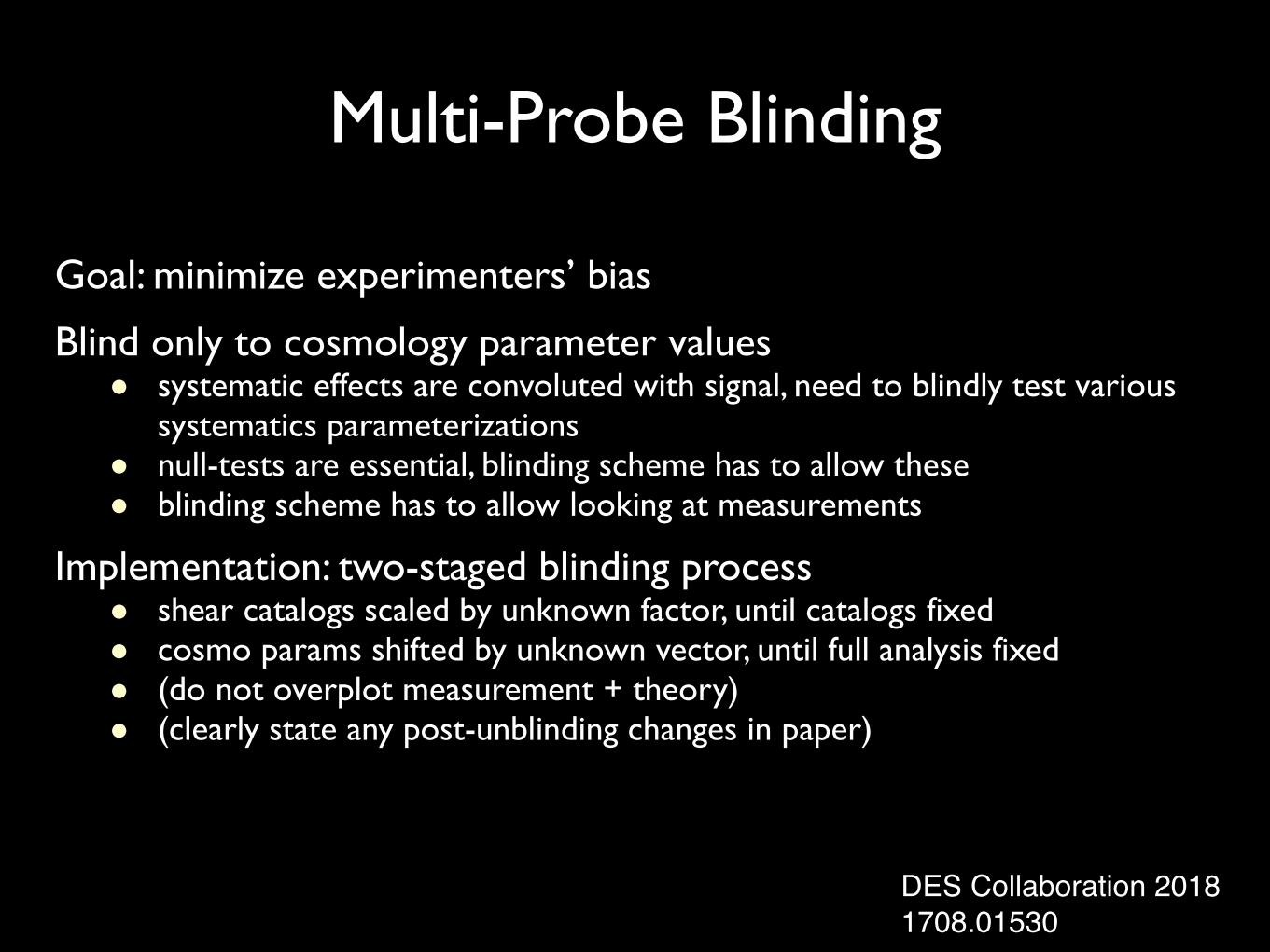
Multi-Probe Blinding

Goal: minimize experimenters’ bias

Blind only to cosmology parameter values● systematic effects are convoluted with signal, need to blindly test various

systematics parameterizations● null-tests are essential, blinding scheme has to allow these● blinding scheme has to allow looking at measurements

Implementation: two-staged blinding process● shear catalogs scaled by unknown factor, until catalogs fixed● cosmo params shifted by unknown vector, until full analysis fixed● (do not overplot measurement + theory)● (clearly state any post-unblinding changes in paper)

DES Collaboration 20181708.01530

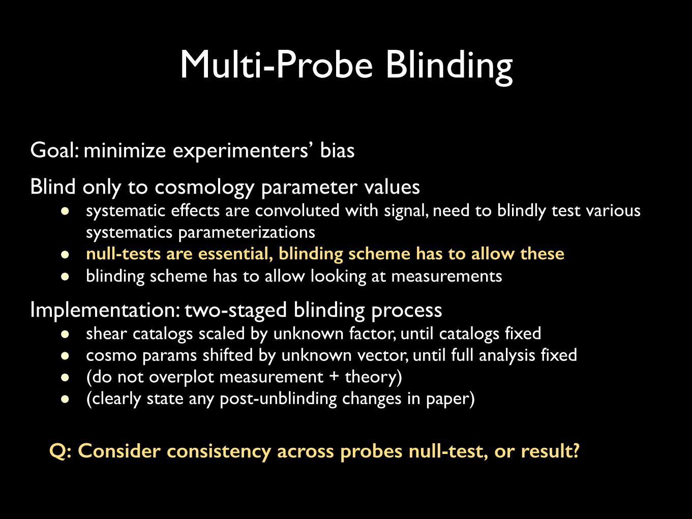
Multi-Probe Blinding

Goal: minimize experimenters’ bias

Blind only to cosmology parameter values● systematic effects are convoluted with signal, need to blindly test various

systematics parameterizations● null-tests are essential, blinding scheme has to allow these ● blinding scheme has to allow looking at measurements

Implementation: two-staged blinding process● shear catalogs scaled by unknown factor, until catalogs fixed● cosmo params shifted by unknown vector, until full analysis fixed● (do not overplot measurement + theory)● (clearly state any post-unblinding changes in paper)

Q: Consider consistency across probes null-test, or result?

DES Y1 Results:LCDM Multi-Probe Constraints

● DES-Y1 most stringent constraints from weak lensing to date

● marginalized 4 cosmology parameters, 10 clustering nuisance parameters, and 10 lensing nuisance parameters

● consistent (Bayes Factor R = 583) cosmology constraints from weak lensing and clustering in configuration space

(DES Collaboration 18)

Matter Density Am

plitu

de o

f Str

uctu

re G

row

th

-> Troxel’s talk for detailed results

Photometric Cosmology Surveys

LSST

LSST!

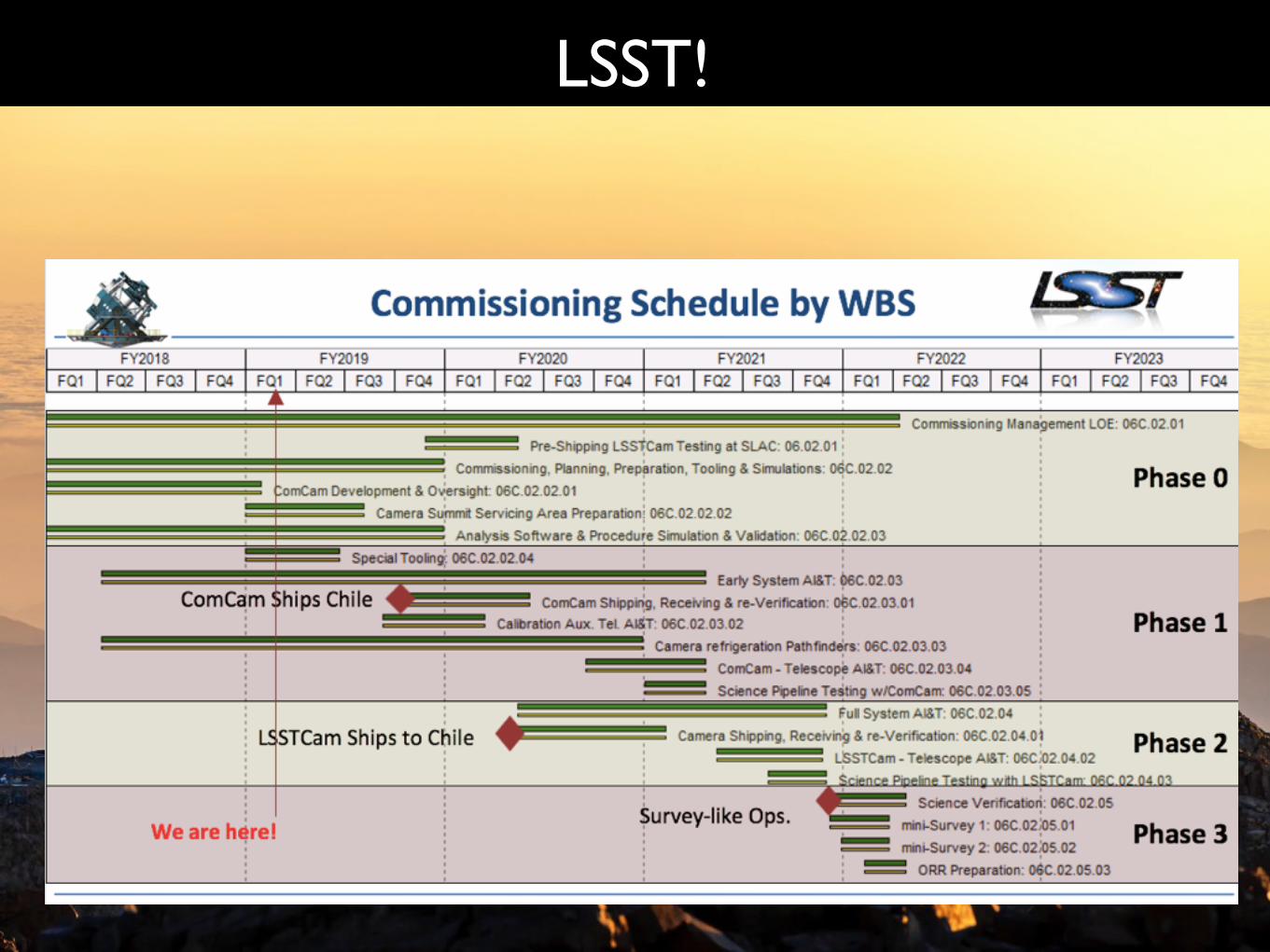
LSST!

Prepare for and carry out cosmology analyses with the LSST survey

• 6 cosmology Science Working Groups (SWG)Galaxy Clustering, Galaxy Clusters, Strong Lensing, Supernovae, Weak Lensing; Theory & Joint Probes

• “Enabeling Analyses” WGs: understand LSST system + systematics

logo/pics

lots of work until first data, lots to learn from ongoing surveys!

3LSST DESC Collaboration Meeting July 2016

Closing Comments

• A big thank you (again!) to the Local Organizing Committee for making

the meeting work so well!

– Elisa Chisari, David Alonso, Ian Shipsey, Jo Dunkley, Aprajita Verma,

Phil Marshall, Joe Zuntz, Matt Jarvis, Pedro Ferreira, Chris Linttot,

Erminia Calabrese and Leanne O'Donnell.

• Thank you everyone for your participation in the meeting!

– Lots of energy and enthusiasm and great interactions in the sessions

– Lots of cross-WG discussions and Task Force hacks

– Junior involvement in talks and discussion

• Three new milestones!

– First meeting outside the UK

– Largest DE School attendance to date

– First collaboration photo

The LSST Dark Energy Science Collaboration

The Power of Multi-Probe Analyses with LSST

LSST DESC Requirements

�0

.20

.00

.20

.4

�w0

�1

.2

�0

.6

0

.0

0

.6

1

.2

�w

a

Clusters Y10SL Y10

Stage IIISN Y10

3x2pt Y10LSST all+Stage III

Figure G2: The forecast dark energy constraints at Y1 (top left) and Y10 (top right; bottom) fromeach probe individually and the joint forecast including Stage III priors. For consistency, the same axesare used on the Y1 and the top Y10 plot, while the bottom Y10 plot is zoomed in further. Note that thesupernova contours appear to be tilted clockwise with respect to typical forecasts shown in the literature,because most papers include a Stage III prior when generating the contour for SN. 68% confidenceintervals are shown in all cases; the plotted quantities �w

0

and �wa are the difference between w0

andwa and their fiducial values of -1 and 0. The contours in this figure for individual probes do not includeStage III priors, so they should only be compared with the individual probe FoM values in Table 6.1 thathave no Stage III prior included.

87

1809.01669, incl. links to data products & Fisher Matrices

• first joint forecast by science collaboration since LSST Science Book (2009)

• based on much more mature survey & analysis assumptions, understanding of systematics

• joint forecasts including cross-correlations (statistical & systematical)

• consider two classes of systematics • self-calibrated, e.g. galaxy bias, intrinsic

alignments, cluster mass-observable relation

• externally calibrated, e.g. photo-zs, shear calibration, photometric calibration

Preparing for Known Systematics

What’s the dominant known systematic for LSST cosmology?

no one-fits-all answer, need to be more specific!

[answer will likely involve galaxy evolution]

• Specify data vector (probes + scales)

• Identify + model systematic effects• find consistent parameterization for all probes

• Constrain parameterization + priors on nuisance parameters• independent observations• other observables from same data set/ split data set

Precision Consistency

Theory Simulations

Forecasts Impact

Parameter Constraints

Model, Priors

Refine Systematics Model

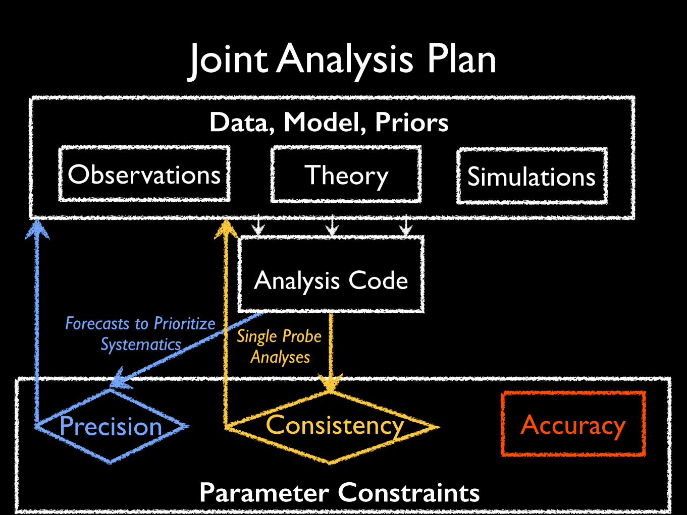
Joint Analysis Plan

Accuracy

Analysis Code

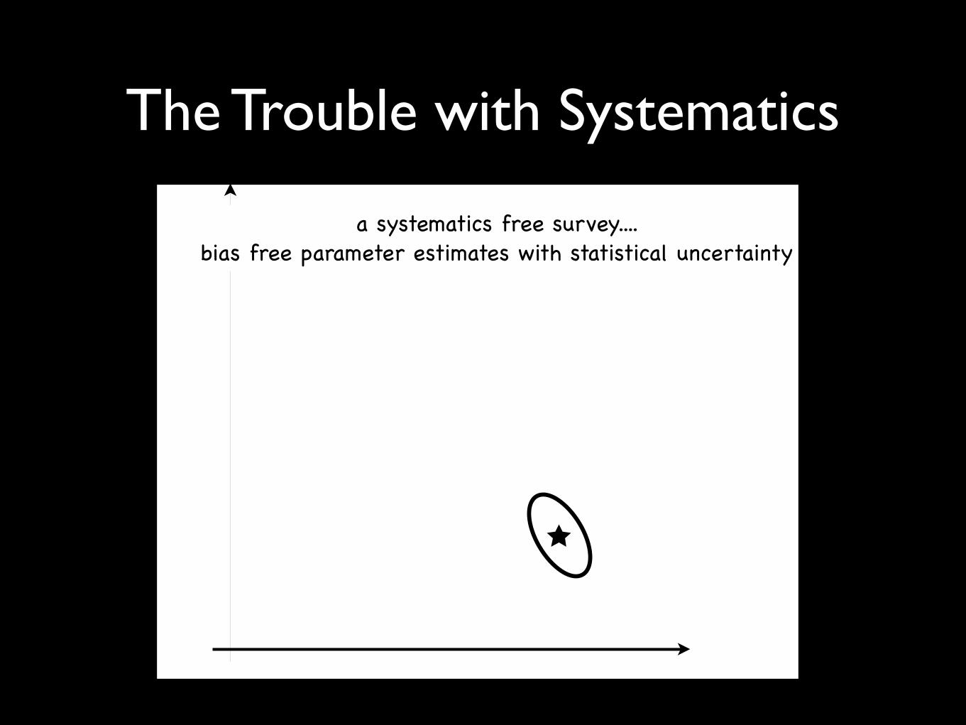
The Trouble with Systematics

a systematics free survey....bias free parameter estimates with statistical uncertainty

The Trouble with Systematics

ignored systematic effect in analysis:parameter bias

The Trouble with Systematics

marginalize systematic effect, correct parameterizationremove parameter bias, increase uncertainty

The Trouble with Systematics

marginalize systematic effect, correct parameterizationremove parameter bias, increase uncertainty

improve priors on nuisance parameters

galaxy evolution: very rich physics compared to primary CMB

what do cosmologists need to know?

• galaxy bias: relation between a galaxy population and matter distribution

Fundamental Physics from Galaxies

CosmoLike 9

3x2pt Rmin=10 Mpc/h3x2pt Rmin=20 Mpc/h

3x2pt Rmin=50 Mpc/h3x2pt Rmin=0.1 Mpc/h, HOD

wp

w a

3x2pt Rmin=10 Mpc/h3x2pt Rmin=0.1 Mpc/h, HOD

3x2pt+cluster Rmin=10 Mpc/h3x2pt+cluster Rmin=0.1 Mpc/h, HOD

wp

w a

Figure 4. Left: Varying the minimum scale included in galaxy clustering and galaxy galaxy lensing measurements. We show the baseline 3x2pt functions,which assumes Rmin = 10Mpc/h (black/solid), and corresponding constraints when using Rmin = 20Mpc/h (red/dashed), Rmin = 50Mpc/h (blue/dot-dashed),Rmin = 0.1Mpc/h (green/long-dashed) instead. For the latter we switch from linear galaxy bias modeling to our HOD implementation. Right: Information gainwhen using HOD instead of linear galaxy bias for 3x2pt (black solid vs dashed contours) in comparison to corresponding information gain when includingcluster number counts and cluster weak lensing in the data vector (violett/dot-dashed vs long-dashed).

cov fiducial cosmology

cov cosmology model 1cov cosmology model2

wp

wa

Figure 5. Change in cosmological constraints when varying the underlyingcosmological model in the covariance matrix. We show three scenarios: 1)the fiducial cosmology (black/solid), 2) fiducial cosmology but a 10% lowervalue in �8 and ⌦m (red/dashed), and 3) fiducial cosmology but changes inthe dark energy parameters, i.e. w0 =�1.3 and wa =�0.5 (blue/dot-dashed).

where

Ci j�gI(l)=�

Z

d�qi�g

�2n j

source(z)

n̄ jsource

dzd�

big(z) fred(z,mlim)P�I(l/�,z,mlim) ,

(26)

with z= z(�). The j dependent term is the normalized distribution ofsource galaxies in redshift bin j, fred is the fraction of red galaxieswhich is evaluated as a function of limiting magnitude mlim = 27,and P�I the cross power spectrum between intrinsic galaxy orienta-tion and matter density contrast.

The IA contamination of our data vector assumes a DEEP2luminosity function (Faber et al. 2007) and the tidal alignment sce-nario described in Blazek et al. (2015); Krause et al. (2016). The

tidal alignment scenario is in good agreement with observations;using the DEEP2 luminosity function should be considered as anupper limit of the strength of IA contaminations.

In Fig. 6 we compare the baseline analysis for cosmic shearand 3x2pt (no IA contamination) to the case where IA contami-nates the data vectors. In the latter case we marginalize over 10nuisance parameters (4 for IA and 6 for luminosity function uncer-tainties, see Krause et al. 2016, for details) to account for the IAcontamination. Although we assume the tidal alignment scenarioas a contaminant, we choose a di↵erent IA model for the marginal-ization (non-linear alignment with the Halofit fitting formula) tomimic a realistic analysis.

We find that in the presence of multiple probes, photo-z, shearcalibration and galaxy bias uncertainties, the assumption of an im-perfect IA model in the marginalization is negligible. As expectedwhen including 10 more dimensions in the analysis the constraintsweaken but again the e↵ect is not severe. Note that the 3x2pt datavector only includes galaxy-galaxy lensing tomography bins forwhich the photometric source redshifts are behind the lens galaxyredshift bin. Hence only a small fraction of source galaxies inthe low-z tail of the redshift distribution contribute an IA signalto galaxy-galaxy lensing. As a consequence the 3x2pt data vectorcontains only marginally more information on IA, and improve-ments in the self-calibration of IA parameters is largely due to theenhanced constraining power on parameters which are degeneratewith IA.

5 Discussion

The first step in designing a multi-probe likelihood analysis is tospecify the exact details of the data vector. This is far from trivial;the optimal data vector is subject to various considerations.

• Science case This paper focusses on time-dependent dark en-ergy as a science case with the fiducial model being ⇤CDM. Ifthere was indication for time-dependence, the data vector can beoptimized (tomography bins, galaxy samples, scales) such that it ismost sensitive to these signatures. The same holds when extending

MNRAS 000, 1–13 (2014)

large scales only

LSST’s constraining power combining WL, and galaxies using

EK, Eifler 17

galaxy evolution: very rich physics compared to primary CMB

what do cosmologists need to know?

• galaxy bias: relation between a galaxy population and matter distribution

Fundamental Physics from Galaxies

CosmoLike 9

3x2pt Rmin=10 Mpc/h3x2pt Rmin=20 Mpc/h

3x2pt Rmin=50 Mpc/h3x2pt Rmin=0.1 Mpc/h, HOD

wp

w a

3x2pt Rmin=10 Mpc/h3x2pt Rmin=0.1 Mpc/h, HOD

3x2pt+cluster Rmin=10 Mpc/h3x2pt+cluster Rmin=0.1 Mpc/h, HOD

wp

w a

Figure 4. Left: Varying the minimum scale included in galaxy clustering and galaxy galaxy lensing measurements. We show the baseline 3x2pt functions,which assumes Rmin = 10Mpc/h (black/solid), and corresponding constraints when using Rmin = 20Mpc/h (red/dashed), Rmin = 50Mpc/h (blue/dot-dashed),Rmin = 0.1Mpc/h (green/long-dashed) instead. For the latter we switch from linear galaxy bias modeling to our HOD implementation. Right: Information gainwhen using HOD instead of linear galaxy bias for 3x2pt (black solid vs dashed contours) in comparison to corresponding information gain when includingcluster number counts and cluster weak lensing in the data vector (violett/dot-dashed vs long-dashed).

cov fiducial cosmology

cov cosmology model 1cov cosmology model2

wp

wa

Figure 5. Change in cosmological constraints when varying the underlyingcosmological model in the covariance matrix. We show three scenarios: 1)the fiducial cosmology (black/solid), 2) fiducial cosmology but a 10% lowervalue in �8 and ⌦m (red/dashed), and 3) fiducial cosmology but changes inthe dark energy parameters, i.e. w0 =�1.3 and wa =�0.5 (blue/dot-dashed).

where

Ci j�gI(l)=�

Z

d�qi�g

�2n j

source(z)

n̄ jsource

dzd�

big(z) fred(z,mlim)P�I(l/�,z,mlim) ,

(26)

with z= z(�). The j dependent term is the normalized distribution ofsource galaxies in redshift bin j, fred is the fraction of red galaxieswhich is evaluated as a function of limiting magnitude mlim = 27,and P�I the cross power spectrum between intrinsic galaxy orienta-tion and matter density contrast.

The IA contamination of our data vector assumes a DEEP2luminosity function (Faber et al. 2007) and the tidal alignment sce-nario described in Blazek et al. (2015); Krause et al. (2016). The

tidal alignment scenario is in good agreement with observations;using the DEEP2 luminosity function should be considered as anupper limit of the strength of IA contaminations.

In Fig. 6 we compare the baseline analysis for cosmic shearand 3x2pt (no IA contamination) to the case where IA contami-nates the data vectors. In the latter case we marginalize over 10nuisance parameters (4 for IA and 6 for luminosity function uncer-tainties, see Krause et al. 2016, for details) to account for the IAcontamination. Although we assume the tidal alignment scenarioas a contaminant, we choose a di↵erent IA model for the marginal-ization (non-linear alignment with the Halofit fitting formula) tomimic a realistic analysis.

We find that in the presence of multiple probes, photo-z, shearcalibration and galaxy bias uncertainties, the assumption of an im-perfect IA model in the marginalization is negligible. As expectedwhen including 10 more dimensions in the analysis the constraintsweaken but again the e↵ect is not severe. Note that the 3x2pt datavector only includes galaxy-galaxy lensing tomography bins forwhich the photometric source redshifts are behind the lens galaxyredshift bin. Hence only a small fraction of source galaxies inthe low-z tail of the redshift distribution contribute an IA signalto galaxy-galaxy lensing. As a consequence the 3x2pt data vectorcontains only marginally more information on IA, and improve-ments in the self-calibration of IA parameters is largely due to theenhanced constraining power on parameters which are degeneratewith IA.

5 Discussion

The first step in designing a multi-probe likelihood analysis is tospecify the exact details of the data vector. This is far from trivial;the optimal data vector is subject to various considerations.

• Science case This paper focusses on time-dependent dark en-ergy as a science case with the fiducial model being ⇤CDM. Ifthere was indication for time-dependence, the data vector can beoptimized (tomography bins, galaxy samples, scales) such that it ismost sensitive to these signatures. The same holds when extending

MNRAS 000, 1–13 (2014)

large scales only

small +large scales

LSST’s constraining power combining WL, and galaxies using

EK, Eifler 17

transformative gain in constraining power(comparable to fsky>1 for large scales only)

iff small scales modeled accurately

The Trouble with Systematics

marginalize systematic effect, imperfect parameterizationresidual parameter bias, increased uncertainty

imperfect IA mitigation examples: EK+16b

Joint Analysis Plan

Precision Consistency

TheoryObservations Simulations

Single Probe Analyses

Forecasts to Prioritize Systematics

Parameter Constraints

Data, Model, Priors

Accuracy

Analysis Code

multi-probe analysis, pass 1 - now what?

Unknown Systematics? vs. New Physics?

Unknown Systematics? vs. New Physics?

• scale dependence?

• dependence on galaxy/cluster selection?

• calibrate with more accurate measurements• spectroscopic redshifts

• low-scatter cluster mass proxies

• galaxy shapes from space-based imaging

• [potentially expensive]

10 Dawson, Schneider, Tyson, & Jee

(a) D2015 J091618.93+29497.3 (b) D2015 J091623.84+294927.7

(c) D2015 J091620.65+29495.9 (d) D2015 J091619.74+294857.3

(e) D2015 J091610.65+294856.5

(g) D2015 J091615.25+294850.4

(f) D2015 J091603.65+295252.3

Figure 6. Visually confirmed ambiguous blends in the Musket Ball Cluster Subaru/HST field (Dawson et al. 2013). For each blend, theSubaru i-band image (left) is shown alongside the HST color image (right; b=F606W, g=F814W, r=F814W). Both images are logarithmi-cally scaled. The ellipses show the observed object ellipticities (red = Subaru, green = HST). The images and green crosshair are centeredon the Subaru ambiguous blend object center. The Subaru pixel scale is 0.2 arcsec/pixel, and the HST pixel scale is 0.05 arcsec/pixel.Panels (a)-(g) show blends selected from the complete sample (available in the electronic edition of the article) to highlight some of thecommon “classes” of ambiguous blends. Panel (a) is an example of a case where two objects with small ellipticity have become ambiguouslyblended in the Subaru image and produced a single detected object with large ellipticity (Subaru object FWHM: 1.600). Panel (b), while lesscommon, it is also possible to have two objects be ambiguously blended together to create a smaller ellipticity object observed in Subaru(Subaru object FWHM: 1.000). Panel (c) is an example of two objects with similar brightness that are ambiguously blended (Subaru objectFWHM: 1.300). Panel (d), two objects need not have similar brightness to generate an ambiguous blend with significantly di↵erent ellipticityproperties compared to that of the brighter object. Even objects in the LSST Gold Sample (i < 25.3) can be significantly a↵ected bythe fainter objects (25.3 < i < 28) in the survey (Subaru object FWHM: 1.200). Panel (e), approximately 25% of ambiguous blends arecomposed of more than two objects (Subaru object FWHM: 1.800). Panel (f), is an example of two objects, likely at di↵erent redshifts(given their di↵erent colors and magnitude), that are ambiguously blended (Subaru object FWHM: 1.400). Panel (g), may be a spiral galaxythat has become fragmented during the reduction of the HST imaging, thus it may be an example an artificial ambiguous blend (Subaruobject FWHM: 1.200). [See the electronic edition of the article for all ambiguous blend panels, Figures 6.1–6.341 ]

Subaru HST-ACSground vs. space-based shape measurements

Dawson+ 2016

Unknown Systematics? vs. New Physics?

• scale dependence?

• dependence on galaxy/cluster selection?

• calibrate with more accurate measurements• spectroscopic redshifts

• low-scatter cluster mass proxies

• galaxy shapes from space-based imaging

• [potentially expensive]

• correlate with other surveys• compare to predicted cross-correlations

• constrain uncorrelated systematics

LSST WL x CMB-S4 lensingcalibrate shear calibration bias

Schaan, EK,+17

11

m 0 m 1 m 2 m 3 m 4 m 5 m 6 m 7 m 8 m 90.000

0.005

0.010

0.015

0.020

0.025

0.030

0.035

0.040

Shea

rbi

as68

%co

nstr

aint

s

LSST shear: �gal�gal

LSST full: gg, g�gal, �gal�gal

Combi2: gg, g�CMB, g�gal

Combi1: �CMB�CMB, �CMB�gal, �gal�gal

LSST full & CMB S4 lensing

LSST requirement

0.2 0.4 0.6 0.7 0.9 1.0 1.2 1.4 1.8 2.4Mean redshift

m 0 m 1 m 2 m 3 m 4 m 5 m 6 m 7 m 8 m 9�0.03

�0.02

�0.01

0.00

0.01

0.02

0.03

IAco

ntam

inat

ion

Combi2: gg, g�CMB, g�gal

Combi1: �CMB�CMB, �CMB�gal, �gal�gal

LSST full & CMB S4 lensing

LSST requirement

0.2 0.4 0.6 0.7 0.9 1.0 1.2 1.4 1.8 2.4Mean redshift

FIG. 5. Left panel: 68% confidence constraints on the shear biases mi for LSST, when self-calibrating them with cosmicshear alone (blue), LSST alone (green), combination 1 (orange), combination 2 (yellow) and the full LSST & CMB S4 lensing(red). The self-calibration works down to the level of LSST requirements (dashed lines) for the highest redshift bins, whereshear calibration is otherwise most dificult. We stress that all the solid lines correspond to self-calibration from the data alone,without relying on image simulations. Calibration from image simulations is expected to meet the LSSt requirements, andCMB lensing will thus provide a valuable consistency check for building confidence in the results from LSST.Right panel: impact of unaccounted intrinsic alignments. The lines show the bias in the self-calibrated value of mi, andthe colored bands show the 68% confidence constraints, corresponding to the curves in the left panel. Intrinsic alignmentcontribution to the shear calibration is present, but still within the 68% confidence region.

VI. SENSITIVITY TO PHOTOMETRIC REDSHIFT UNCERTAINTIES

In Sec. IV, we showed that CMB S4 lensing can calibrate the shear from LSST, assuming that the photometricredshift uncertainties are under control. In this section, we ask whether this assumption was crucial or not. Wetherefore vary the priors on source and lens photo-z uncertainties and re-run our forecast. Fig. 8 shows that theshear calibration is mildly dependent on the source photo-z uncertainties (left panel), and very insensitive to the lensphoto-z uncertainties (right panel). However, we have not taken into account photo-z catastrophic failures in thisanalysis.

VII. APPLICATION TO SPACE-BASED LENSING SURVEYS: EUCLID AND WFIRST

In this section, we reproduce our main forecast on shear calibration in the cases of Euclid and WFIRST. Ourassumptions and results are summarized in Fig. 9 and 10. CMB lensing from S4 can calibrate the shear for the 5Euclid source bins down to 0.4% � 1.4%, and for the 10 WFIRST source bins down to 0.6% � 3.2%. These resultsare clearly very encouraging.

VIII. CONCLUSION

[Eli: Comment on possible degeneracies between shear calibration and more realistic photo-z uncertainties.]Weak gravitational lensing of galaxy images is a potentially powerful probe of the geometry and growth history

of the universe, and therefore of the properties of dark energy, the neutrino masses and possible modifications togeneral relativity. Realizing the full potential of upcoming weak lensing surveys requires an exquisite understandingof systematics e↵ects, such as photometric redshift uncertainties, intrinsic alignments, theoretical uncertainties relatedto non-linear growth and baryonic e↵ects, and shear multiplicative bias. Because these systematic uncertainties areso challenging, alternative methods to calibrate are valuable: they provide redundancy and contribute to buildingtrust in the results. In this paper, we focused on calibrating the shear multiplicative bias from LSST by using CMB

multi-probe analysis, pass 1 - now what?would comparison with Planck results change this plan?

Planck best fit

Unknown Systematics? vs. New Physics?

Joint Analysis Plan

Precision Consistency Accuracy

TheoryObservations Simulations

Combined ProbesAnalysis

Single Probe Analyses

Forecasts to Prioritize Systematics

Parameter Constraints

BlindingAnalysis Code

Data, Model, Priors

Cosmology Analysis Parameters

Cosmology Parameters

5%

25%

70%

Sample CutParameters

“Systematics Parameters”

• observational systematics• survey specific

• astrophysical systematics• probe + survey specific

Cosmology Parameters

5%

25%

70%

Sample CutParameters

“Systematics Parameters”

• observational systematics• survey specific

• astrophysical systematics• probe + survey specific

sample cuts + systematics highly interconnected 95% systematics…

Cosmology Analysis Parameters

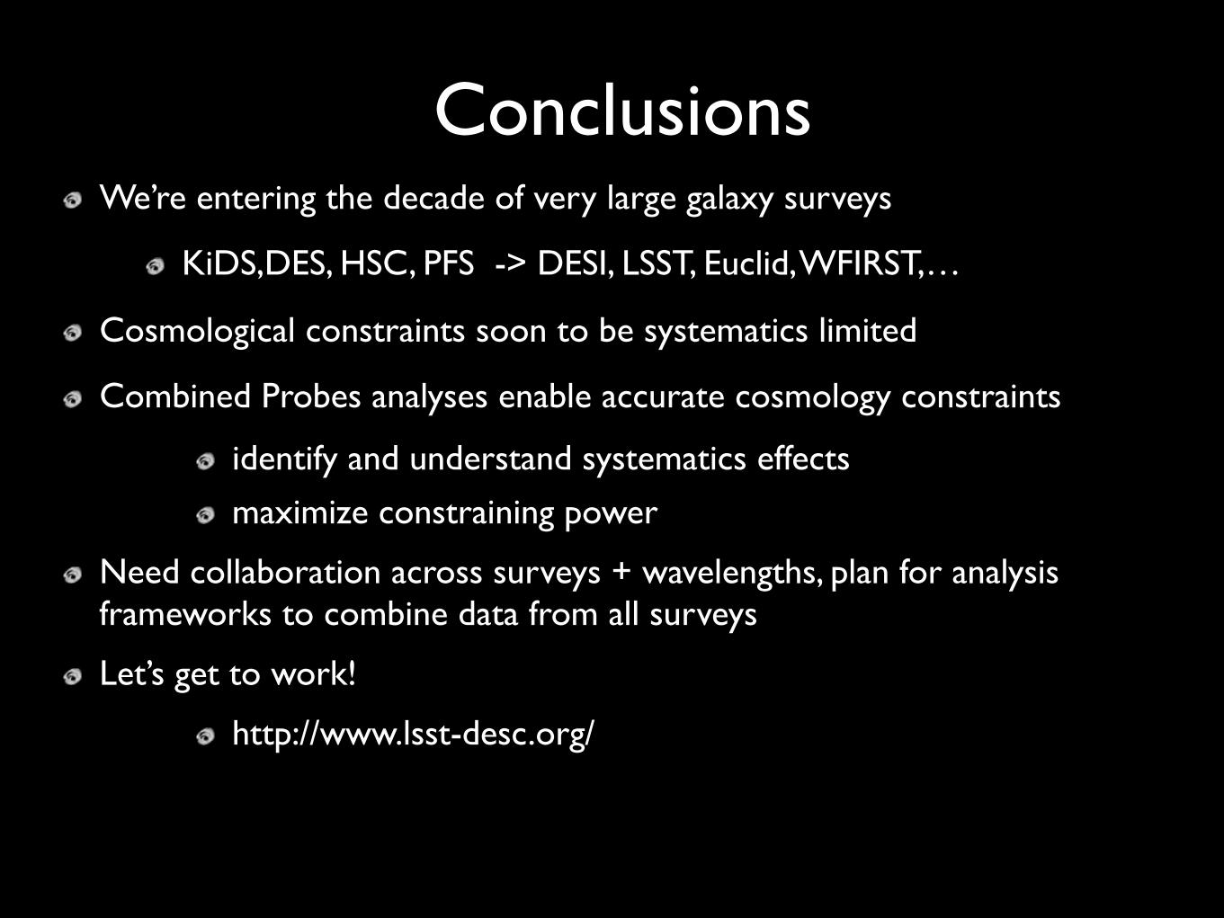
ConclusionsWe’re entering the decade of very large galaxy surveys

KiDS,DES, HSC, PFS -> DESI, LSST, Euclid, WFIRST,…

Cosmological constraints soon to be systematics limited

Combined Probes analyses enable accurate cosmology constraints

identify and understand systematics effects

maximize constraining power

Need collaboration across surveys + wavelengths, plan for analysis frameworks to combine data from all surveys

Let’s get to work!

http://www.lsst-desc.org/