Electronic copy available at: http://ssrn.com/abstract=1649790Electronic copy available at: http://ssrn.com/abstract=1649790

The Origins of Savings Behavior∗

Henrik Cronqvist and Stephan Siegel†

This version: July 30, 2010

Abstract

What are the origins of individual savings behavior? Using data on identical and fraternal twins matched

with data on their savings behavior, we find that an individual’s savings propensity is governed by both

genetic predispositions, social transmission from parents to their children, and gene-environment interplay

where certain environments moderate genetic influences. Genetic variation explains about 35 percent of

the variation in savings rates across individuals, and this genetic effect is stronger in less constraining, high

socioeconomic status environments. Parent-child transmission influences savings for young individuals and

those who grew up in a family environment with less competition for parental resources. Individual-specific

life experiences are a very important explanation for behavior in the savings domain, and strongest in urban

communities. In a world progressing rapidly towards individual retirement savings autonomy, understanding

the origins of individuals’ savings behavior are of key importance to economists as well as policy makers.

∗We are thankful for comments from seminar participants at the China Europe International Business School,Financial Research Association, and Singapore International Conference on Finance, and valuable discussions withPeter Bossaerts, Darrell Duffie, Daniel Hamermesh, David Hirshleifer, Greg Hess, Andrew Karolyi, Camelia Kuhnen,Andy Lo, Ed Rice, Jay Ritter, Frank Yu, and Paul Zak. We thank Jack Goldberg at the University of WashingtonTwin Registry for advice, Florian Muenkel for research assistance, and Kara Ralston for editorial assistance. Weacknowledge research funding from the Financial Economics Institute and the Lowe Institute of Political Economy atClaremont McKenna College, and the Global Business Center and the CFO Forum at the University of Washington.This project was pursued in part when Cronqvist was visiting the Institute for Financial Research (SIFR), which hethanks for its hospitality. Statistics Sweden and the Swedish Twin Registry (STR) provided the data for this study.STR is supported by grants from the Swedish Research Council, the Ministry of Higher Education, AstraZeneca, andthe National Institute of Health (grants AG08724, DK066134, and CA085739). The project has been reviewed andapproved by the Swedish Twin Registry, the Ethics Review Board for the Stockholm region, and Statistics Sweden.Any errors or omissions are our own.†Cronqvist: McMahon Family Chair in Corporate Finance, George R. Roberts Fellow, and Associate Professor of Fi-

nancial Economics, Claremont McKenna College, Robert Day School of Economics and Finance (hcronqvist@cmc.edu);Siegel: Assistant Professor of Finance, University of Washington, Michael G. Foster School of Business (ss1110@uw.edu).

Electronic copy available at: http://ssrn.com/abstract=1649790Electronic copy available at: http://ssrn.com/abstract=1649790

I Introduction

There is enormous variation across individuals in terms of wealth accumulated at retirement age, even

among those with relatively similar lifetime incomes. Researchers have found that this variation can

not easily be explained by “chance” events (e.g., inheritances, health status) or by asset allocation

choices (e.g. Venti and Wise (1998, 2000) and Bernheim et al. (2000)). Instead, savings behavior,

i.e., the choice to save or spend earlier in life, seems to be a much more important determinant

of variation in wealth accumulation.1 These findings raise a very fundamental question: Where

does an individual’s savings behavior originate from? What makes one individual a “spender” while

another individual, with very similar income and other socioeconomic characteristics, saves a large

portion of his or her income?

One can, of course, take different empirical approaches to addressing these questions, and we

are not the first to estimate determinants of individuals’ savings behavior.2 The empirical approach

of our work, which has not been previously explored in the literature, is to decompose the variation

in savings behavior across individuals into genetic versus environmental influences (e.g., social

transmission of behavior from parents to their children), and to examine gene-environment interplay.

This approach will result in a better understanding of where individuals’ savings behavior originate

from. Our analysis relates to an area of research at the intersection of economics and biology.

Several prominent economists have long recognized a great potential for research in this area (e.g.,

Marshall (1920), Becker (1976) and Hirshleifer (1977)),3 but it is with the recent appearance of

large data sets of individuals matched with their economic behaviors that empirical research in this

area has also become possible.

In a standard economic model, differences in savings behavior across individuals are related

to differences in preferences. Several economic theorists have recently proposed that the existence

and general shape of such preferences are the outcome of natural selection (e.g., Rogers (1994),

Robson (2001), Netzer (2009), and Brennan and Lo (2009)), implying that preferences, and thus

1Friedman (1953) concludes that “a large part of the existing inequality of wealth can be regarded as produced bymen to satisfy their preferences” (p. 290).

2We refer to Browning and Lusardi (1996) for an extensive review of micro-level research on savings behavior.3Marshall (1920) went as far as arguing that “economics is a branch of biology broadly interpreted” (p. 772)

1

savings behavior, are at least partially genetically determined. There is confirming evidence that

preferences with respect to both risk and time are in part genetic (e.g., see Kuhnen and Chiao

(2009), Barnea et al. (2010), and Cesarini et al. (2009b) for risk preferences, and Eisenberg et al.

(2007) and Carpenter et al. (2009) for time preferences). Other economists have emphasized that

behaviors and preferences may be socially (as opposed to genetically) transmitted from parents to

their children (e.g., Cavalli-Sforza and Feldman (1981), Bisin and Verdier (2000, 2008), and Dohmen

et al. (2008)). Casual evidence indeed seems to suggest that some parents give their children a piggy

bank, open a savings account, and instill the importance of being frugal, while other parents do not.

Such parent-child socialization imply that children adopt their parents’ consumption-savings choices

by learning. Such socialization has been found to be empirically important for other economic

behaviors than savings (e.g., Bisin and Verdier (2000), Bisin et al. (2004), and Fernandez et al.

(2004)). Finally, Knudsen et al. (2006) argue that genes and environmental factors interact in

important ways. Our empirical approach allows us to quantify the proportion of the total variation

across individuals in the propensity to save that is attributable to genes versus parent-child social

transmission, accounting for gene-environment interactions.

There are several reasons why it is important for economists to uncover the origins of individuals’

choices about savings. First, most industrialized countries are in the process of rapidly moving

away from pensions or defined benefit retirement plans, meaning that individuals are increasingly

responsible for their own savings. As we progress towards more autonomy in the domain of savings,

it is increasingly important and relevant to explain why some individuals choose to save while others

do not.4 Second, work in this area has potentially important public policy implications, in particular

for economists’ evaluations of the sensitivity of savings behavior to policy initiatives. Bernheim

(2009) recently concluded: “The discovery of a patience gene could shed light on the extent to which

correlations between the wealth of parents and their children reflect predispositions rather than

environmental factors that are presumably more amenable to policy intervention” (p. 14).

Our research is related to work by Charles and Hurst (2003) and Knowles and Postlewaite (2004)

that document significant parent-child similarities in savings behavior. Charles and Hurst (2003)

4A large literature studies the effects of financial literacy on savings behavior (e.g., Lusardi (1998), Bernheim et al.(2001), and Bernheim and Garrett (2003)).

2

show that the age-adjusted elasticity of child wealth with respect to parental wealth is 0.37 (before

bequests). While similarity in income explains about half of the intergenerational wealth elasticity,

they speculate that similar savings propensities among parents and their children is another possible

factor. Knowles and Postlewaite (2004) show that parents who save more than predicted by their

income and other socioeconomic characteristics, on average, have children that behave similarly.

Both these studies are important in that they document that parents pass on savings propensities

to their children, but they do not examine whether the origins of savings behavior are genetic versus

social, an important distinction from the perspective of modeling behavior and the sensitivity of

savings behavior to policy initiatives.5

In contrast to previous research on consumption-savings choices, we decompose the variation in

the individual propensity to save into genetic and environmental components. We do this by applying

empirical methods developed by quantitative behavioral genetics researchers, in combination with

data on the savings behavior of pairs of identical and fraternal twins.6 Our data on twins are

from the Swedish Twin Registry, the world’s largest research database of twins. These data are

matched by Statistics Sweden with income and net worth data from these individuals’ tax filings.

Using changes in net worth and disposable income, we determine an individual’s savings rate. The

decomposition of that rate into genetic and environmental factors builds on an intuitive insight:

identical twins share 100 percent of their genes while the average proportion of shared genes is only

50 percent for fraternal twins, so if identical twins have significantly more similar savings behavior

than fraternal twins, then there is evidence that the propensity to save, at least partly, originates

from an individual’s genetic composition.

We find that innate genetic propensities explain about 35 percent of the variation in savings

propensities across individuals. Men’s savings behavior is explained more by their genes compared to

5A large literature in economics has studied parent-child similarities in other domains than savings behavior.(Bowles and Gintis, 2002) report that socioeconomic status is much more persistent across generations than previouslythought. Borjas (1992) and Solon (1992) find a positive and significant intergenerational correlation in income. Chitejiand Stafford (1999) examine asset allocations, and find that children (as young adults) are more likely to own stockswhen their parents owned such financial assets. Mulligan (1999), Black et al. (2005), and Guell et al. (2007) provideevidence of significant intergenerational transmission with respect to education.

6Several studies in economics have examined data on twins, e.g., Behrman and Taubman (1976), Taubman (1976),Ashenfelter and Krueger (1994), and Ashenfelter and Rouse (1998). Others have used adoption data to address relatedquestions, see for example Sacerdote (2002) and Bjorklund et al. (2006).

3

women, whose behavior is more influenced by individual-specific life experiences. These results are

robust to using several alternative savings rate measures and model specifications. We conclude that

each individual is endowed with a genetic code that affects his or her savings behavior through life,

an effect that does not decay with the gain of own life experience. We also find that parents transmit

savings behavior to their children outside of a genetic mechanism, in particular for the youngest

individuals in our sample and for those who grew up in a family environment with less competition

for parental resources (measured by the presence of non-twin siblings in the family). Finally, we

find evidence of important gene-environment interplay, involving an individual’s current as well as

childhood and early adolescence environments as moderators of genetic predispositions. Generally,

we find that genetic variation plays a more prominent role in less constraining environments, as for

example characterized by education or wealth. That is, social transmission and other environmental

factors affect variation in savings behavior, both directly and through gene-environment interactions.

The paper is organized as follows. Section II reviews related research. Section III describes

our data sources, defines the savings measures and other variables, and reports summary statistics.

Section IV reports our initial results on genetic and social transmission of savings behavior as well

as robustness checks. Section V reports results related to gene-environment interactions. Section VI

discusses what the evidence does and does not mean. Section VII concludes.

II Related Research

Since the seminal work by Modigliani and Brumberg (1954), the lifecycle savings model has been the

framework through which economists have generally studied individuals’ saving and consumption

choices: individuals save to smooth consumption over time. Individuals who seem to be more

patient have indeed been found to save more (e.g., Lusardi (2001)). The standard model has been

extended to account for, e.g., precautionary savings and bequest, suggesting that differences in

consumption-savings choices across individuals are related to: (i) differences in preferences with

respect to risk, time, and bequest, and (ii) differences in circumstances such as income volatility or

4

borrowing constraints.7 Of course, circumstances are partly endogenously determined as a function

of the same underlying preference parameters.

Empirical evidence documents substantial variation in savings behavior across individuals. Some

of that variation appears to be related to differences in circumstances,8 while Lusardi (1998, 2001)

finds that differences in risk, time, and bequest preferences also seem to matter as predicted.

Finally, research on individuals’ risk preferences has found significant cross-sectional variation,

persistence, and behavioral consistency across domains (e.g., Barsky et al. (1997) and Donkers et al.

(2001)).9 There is also evidence of significant variation in time preferences across individuals (e.g.,

Warner and Pleeter (2001) and Harrison et al. (2002)).

We now discuss the extent to which we expect this variation in preferences, and thus in savings

behavior, to be caused by genetic differences versus differences in parent-child social transmission

(i.e., learning from parents).10

A Genetics and Savings Behavior

If savings behavior is found to be heritable, we would in standard economic models expect the

genetic transmission to operate through individuals’ preferences. Do we have reason to expect that

risk and time preferences are, at least partly, innate? An increasing number of economic theorists

would suggest that the answer is yes. For example, Rogers (1994), Robson (1996), Netzer (2009),

Robson and Samuelson (2009), and Brennan and Lo (2009) all propose that the existence and

general shape of preferences are the outcome of natural selection. For this to be the case, preferences

must be at least partially genetically determined. Of course, evolution often results in no variation

7For precautionary savings models, see, e.g., Leland (1968), Kimball (1990), Skinner (1988), Deaton (1991), Carroll(1992) and Hubbard et al. (1995). For models that incorporate bequest motives, see Becker and Tomes (1976) andBernheim et al. (1985).

8See for example Hubbard et al. (1994), Lusardi (1998), and Carroll and Samwick (1997, 1998).9Kimball et al. (2009) report significant cross-sectional variation in survey measures of risk preferences, controlling

for measurement error. Sahm (2007) reports that persistent differences across individuals account for a vast majorityof the cross-sectional variation in risk aversion, i.e., risk preferences are very persistent. Barsky et al. (1997) reportevidence of consistency in risky behaviors across domains: those who are less risk averse are found to smoke more,drink more, have no insurance, choose riskier employment, and hold more stocks compared to other individuals.Reuben et al. (2010) find that discount rates elicited with monetary and primary rewards (chocolate) are significantlypositively correlated.

10While we are not aware of direct evidence of genetic variation with respect to bequest motives, Rushton et al.(1986) document that altruism is up to 50 percent heritable and Rodgers et al. (2001) find that variation with respectto the number of children an individual has a significant genetic component.

5

across individuals at all. For example, all humans are genetically coded to have two eyes (absent

genetic defects). So, to the extent that variation in savings behavior is genetic, it must be that

such variation is optimal in the population (“frequency dependent selection”) or irrelevant from an

evolutionary perspective. That is, variation in risk aversion or time preferences across individuals

either improves the survival rate of the species or does not correlate with the survival of the species

at all.11

A.1 Risk Preferences

Emerging evidence in economics and finance suggests that an individual’s risk aversion has a

significant genetic component. Recent studies use data on twins to estimate the genetic component

of risk preferences using individual-level data from the financial domain (e.g., Barnea et al. (2010)

and Cesarini et al. (2009b)). For example, Barnea et al. examine individuals’ overall financial

portfolios and find that about one third of the cross-sectional variation in the share in equities across

individuals is explained by an innate genetic factor. In a standard frictionless model, differences in

risk preferences cause cross-sectional variation in the share in equities. The Barnea et al. (2010)

evidence may therefore be interpreted as reflecting genetic variation in risk preferences across

individuals. Experimental research on genes and risk aversion confirms these findings (e.g. Cesarini

et al. (2009a) and Zyphur et al. (2009)).

Another important string of recent research at the intersection of economics and genetics has

examined which specific genes are responsible for risky behaviors. This work starts with the

well-established result that, for some individuals, taking more risk results in more and longer-lasting

production of “feel-good” neurotransmitters, e.g., dopamine.12 Moreover, gene-mapping studies

have found which specific genes regulate this dopamine production. Those with genes such as the

7-repeat allele (7R+) of the dopamine receptor D4 (CRD4) have been found to find risky behaviors

more rewarding.13 There also exists some evidence that testosterone can affect risk taking behavior

11For broad reviews of research at the intersection of neuroscience, genetics, and economics, see, e.g., Camerer et al.(2005) and Benjamin et al. (2008).

12See Caplin and Dean (2008) for work on the axioms behind the “dopaminergic reward prediction error” hypothesis.13For experimental research on dopamine receptor genes and risk preferences, see Carpenter et al. (2009) and Dreber

et al. (2010).

6

(see e.g. Sapienza et al. (2009)). In the financial domain, Kuhnen and Chiao (2009) and Dreber

et al. (2009) elicit risk preferences using experiments and find that those with certain genes have

a larger propensity to take risk than those who do not have those genes.14 These studies reveal

which specific genes are related to risk preferences, but they cannot inform us about the relative

importance of genes versus social transmission of behavior or the proportion of the variation in

behavior attributable to these mechanisms.15

A.2 Time Preferences

In his seminal “marshmallow experiment”, psychology researcher Walter Mischel found significant

variation across pre-school children in their propensity to forego an immediate reward (i.e., consuming

a marshmallow) for a larger, but delayed, reward (i.e., consuming two marshmallows when the

experimenter returned to the room). Most importantly, subsequent research on these very same

children has shown that the time preferences estimated at an early age using marshmallows explain

a series of important economic outcomes in life, including SAT scores and educational attainment,

social competence, and even drug abuse (e.g., Mischel et al. (1989)). That is, those who are more

patient, and do not immediately consume the marshmallow, also have better ability to invest in,

e.g., education.

The evidence raises question of whether individual time preferences are genetic. Recent gene-

mapping studies indeed suggest that individuals’ discount rates have a genetic component. For

example, Eisenberg et al. (2007) use the “delay discounting method” to elicit individuals’ time

preferences. This method poses a series of choices between smaller intermediate and larger delayed

monetary rewards (e.g., Fuchs (1982)) and with different durations of a delay, for example “Would

you prefer to have $500 today or $1,000 in five years?” Most importantly, they find that the DRD2

TaqI A and DRD4 VNTR genes cause significant variation in individual discounting.

14Zhong et al. (2009) show that individuals with the Monoamine Oxidase A (MAOA) gene prefer lotteries with asmall probability of a very substantial payoff.

15Contrary to early beliefs among many geneticists, gene-mapping has had a difficult time pinpointing down theexact genes responsible for common diseases such as cancer and Alzheimer’s. For a recent popular press account ofthe challenges of gene-mapping, see, e.g., Wade (2010).

7

B Parent-Child Social Transmission of Savings Behavior

Social transmission is another potentially important mechanism behind parent-child similarities in

savings behavior. The specific social transmission mechanism we study in this paper is “direct vertical

socialization,” i.e., transmission of behavior from parents to their children (e.g., Cavalli-Sforza and

Feldman (1981), Boyd and Richerson (1985), and Richerson and Boyd (2005)).16

Bisin and Verdier (2001) provide an economic model of vertical parent-child socialization. A

common assumption in such models is that children are born without defined preferences, and they

are first exposed to their parents’ socialization. Parents have a technology, “parenting,” which

transmits their own preferences to their children. If parent-child socialization is not successful, the

child is in these models affected by a random role model (representing peers, teachers, etc.) in the

population. Altruism makes parents exert costly effort to socialize their children, but this altruism is

paternalistic in the sense that parents prefer to socialize their children to their very own preferences.

Models with these assumptions have been used to explain parent-child social transmission of, for

example, ethnic, religious, and labor supply preferences (e.g., Bisin and Verdier (2000), Bisin et al.

(2004), and Fernandez et al. (2004)). These models of social transmission of behavior from parents

to their children may extend to risk and time preference parameters, though there is not much

evidence of transmission at such a detailed level (e.g., Bisin and Verdier (2000, 2008)).

The questions whether parent-child social transmission influences behavior, i.e., whether parenting

matters, has been researched for decades, but there is no agreement on an answer. Economists

have only recently started to research related questions, and the extent to which parents influence

outcomes of importance to economists is still an open question. In a controversial article, Harris

(1995) challenges the notion that parents significantly affect the behavior of their children. She

concludes based on evidence from behavioral genetics that parents have little long-lasting effects on

their children’s personality. By contrast, Knudsen et al. (2006) provide evidence that exposure, in

particular in early life, to certain risk factors, such as poverty and limited parent education, impact

children’s adult life. Maccoby (2000) attempts to reconcile these views and suggests that the same

parental influence might have different effects on children whose genetic make-up is different. She

16In this paper, we do not study “oblique socialization,” i.e., socialization outside the family, which takes place insociety at large though imitation and learning from others in the population.

8

also points to the potential importance of gene-environment interactions, where genetic expression

depends, for example, on the quality of the parenting.

Based on the reviewed research, we predict that savings behavior is partly governed by an

individual’s genes and parent-child socialization, and also potentially by gene-environment interplay

such that certain environments moderate genetic influences.

III Data

A Data Sources

We use a unique data set with a large number of twins. The data set was constructed by matching

cross-sectional information from the Swedish Twin Registry (STR) with annual financial as well as

demographic data from individuals’ tax filings.

For tax purposes, Sweden, like many other countries, collects detailed information on an

individual’s income. Until 2006, Swedish taxpayers were also subject to a 1.5 percent wealth tax. By

law, financial institutions were therefore required to report to the government detailed information

about assets owned by individual tax payers. The combination of data on income, asset ownership,

and outstanding debt provides an unusually detailed and complete characterization of financial

decisions of Swedish households.17

Based on an individual identifier, personnummer, Statistics Sweden matched the income and

wealth data for all twins that are on file with the STR. The STR is the world’s largest twin registry

and provides high quality data for researchers Lichtenstein et al. (2006). While all twins in Sweden

are registered at birth, the STR has collected extensive additional data through interviews and

surveys in which between 60 and 70 percent of the twins have participated.18 Most important for

our study is the zygosity of a twin pair: monozygotic, or identical, twins are genetically identical,

17Calvet et al. (2007, 2009) use these data to study portfolio choices of Swedish investors.18The STR data used in this study was obtained through the “SALT” (Screening Across Lifespan Twin) study

for twins born between 1886 and 1958 and through the “STAGE” (Swedish Twin Studies of Adults: Genes andEnvironment) study for those born between 1959 and 1985.

9

while dizygotic, or fraternal, twins are genetically different.19

B Measuring Savings Behavior

While our data set contains detailed information on the twins’ income as well as asset ownership,

we do not have a pre-defined measure of their savings behavior. Moreover, as Dynan et al. (2004)

point out, there are several possible ways of measuring individuals’ savings rates. Conceptually, we

characterize an individual’s savings behavior by the proportion of disposable income in a period that

is not consumed, but instead invested (or saved) for future consumption or bequest. For comparison

purposes, this amount is scaled by the disposable income and then referred to as the Savings Rate.

In principle, the amount saved during a period can be measured by the change in an individual’s

net worth during that period. Under such a broad savings measure, unrealized expected and

unexpected capital gains or losses, for example in the form of changes in an individual’s house value,

are included in the amount saved, as long as such capital gains are not converted into consumption

through increased leverage. For this measure, all capital gains and losses would be included in the

disposable income. Alternatively, savings could be defined much more narrowly by excluding any

capital gains and by focusing on the disposable income that is actively set aside and not consumed

in a given period.

In this study, we propose a definition of saving that starts with the change in an individual’s net

worth between the end of 2002 and the end of 2006, but eliminates – in the case of homeowners –

unrealized capital gains or losses related to the individual’s home. Thus, the Savings Rate (si) for

individual i is defined as:

si =Net Worth2006 − Net Worth2002 − (Home2006 − Home2002)∑2006

t=2003 Disposable Incomet(1)

Net worth is defined as the sum of the value of all financial assets, including bank accounts,20 the

19Zygosity is based on questions about intrapair similarities in childhood. One of the survey questions is: Were youand your twin partner during childhood “as alike as two peas in a pod” or were you “no more alike than siblingsin general” with regard to appearance? This method has been validated with DNA as having 98 percent or higheraccuracy. For twin pairs for which DNA sampling has been conducted, zygosity status based on DNA analysis is used.

20Cash in bank accounts with a balance of less than SEK 10,000 (or for which the interest was less than SEK 100during the year). However, Statistics Sweden’s estimations suggest that 98 percent of all cash in bank accounts isincluded in the data.

10

value of all real estate assets, and the value of other assets less outstanding debt. Disposable income

is calculated as the sum of labor income, investment income, income from a private business, early

retirement income, as well as transfer payments such as child support and unemployment benefits

less income taxes and alimony payments. Since the amount saved is calculated over a four year

period, disposable income used in the calculation of the savings rate represents the total disposable

income for years 2003 through 2006.

Unrealized capital gains or losses are not included in the disposable income, but realized capital

gains or losses are taxable and therefore generally reported as investment income. Because we

generally do not know at which price individuals have purchased their home, we cannot calculate

the capital gain that at the time of the sale is included in the disposable income. We therefore drop

all homeowners that have moved over the four-year period or those whose homeowner status has

changed over the four-year period.21

C Sample Selection and Summary Statistics

While Statistics Sweden is able to identify over 50,000 individual twins with tax records in 2006, we

impose several criteria that reduce the number of observations in our final data set. Specifically, we

require that net worth is non-missing in 2002 and 2006 and that the four-year average net worth

(calculated as the average of net worth at the end of 2003, 2004, 2005, and 2006) is positive. We

drop all twins whose four-year average disposable income (again calculated as the average of the

disposable income in 2003, 2004, 2005, and 2006) is below SEK 10,000 (approximately $1,400 at an

average exchange rate of SEK 7.20 per dollar).22 To avoid changes in net worth unrelated to savings

decisions made by the individual, we exclude twins whose civil status has changed, and similarly,

homeowners who have moved between the end of 2002 and the end of 2006. We also restrict our

sample to twins that are at least 18 years old, but at or below age 65 at the end of 2006.23 We do

so to focus on twins that are likely to have a significant income from which to save as well as the

motive to save for retirement. Finally, we drop individuals in the bottom and top one percent of the

21We identify movers by observing changes in their four-digit municipality code.22We require at least three non-missing observations for the calculation of any four-year average.23The official retirement age in Sweden is 65, but we observe age only at the end of the year and hence include

twins that turned 65 at some point in 2006.

11

distribution of the savings rate to ensure that our results are not affected by outliers. As we discuss

below in more detail, our estimation approach requires complete pairs of identical and fraternal

twins. Our final data set of 17,630 observations therefore only contains complete twin pairs.

Panel A of Table 1 reports the number of twins included in our data set by zygosity and gender.

Out of 17,630 twins, 5,142 (29%) are identical, while 12,488 (71%) are fraternal twins. That is,

fraternal twins are more common than identical twins. Moreover, we see that opposite-sex twins

are the most common twin type (39%), and identical male twins are the least common one (12%)

in our data set. The evidence in the table on the relative frequency of different types of twins is

consistent with that from other studies which use large samples of twins.

Panel B reports summary statistics for several individual characteristics.24 Detailed definitions

for all variables are provided in Appendix Table A1. Unless stated otherwise, all variables refer

to 2006. Comparing identical and fraternal twins, we see that they are quite similar. The average

age of identical twins is about 49 years, while the average age of fraternal twins is 53 years. The

civil status is also similar across twin types: over 50% are married, about 10% are divorced and

only about 1% are widowed. 15 to 20% of the twins in our sample have a high school degree, while

about half have a college or equivalent degree. About a third of the twins in our data set have an

advanced graduate or equivalent degree. The majority of twins, more than 70%, are homeowners in

2002 and 2006. The average annual disposable income, averaged over 2003, 2004, 2005, and 2006,

and expressed in U.S. dollars, is $33,000 to $34,000, with similar dispersion among identical and

fraternal twins. The average net worth is slightly lower for identical twins (about $113,000) than for

fraternal twins (about $119,000), while the dispersion is the same for both groups. Conditional on

home ownership, the average value of owner-occupied houses in 2006 is approximately $155,000.

Panel C reports details on the savings behavior of the twins in our data set. Between the end of

2002 and the end of 2006, net worth changed on average by about $62,000 for identical and $66,000

for fraternal twins. Part of that increase in net worth is due to increases in real estate values. Using

home values for the 12,903 twins that are homeowners, we observe an increase in median home

prices by approximately 33% between 2002 and 2006. Averaging across all twins, homeowners and

24The size of the samples (N) differs across rows because of data availability.

12

non-homeowners, we see that about $40,000 of the change in net worth is related to change in

home prices. Adjusting the change in net worth by this change in the home value and scaling this

difference by the disposable income over the four years yields our savings rate. For identical twins

the average saving rate is 15%, while it is 19% for fraternal twins. The median saving rates are

lower for both groups, and about 10%. Finally, the dispersion across identical twins (48%) and

across fraternal twins (50%) is very similar.

Dynan et al. (2004) study a similar savings rate measure for the U.S. using micro data from

the Survey of Consumer Finance (SCF) and the Panel Study of Income Dynamics (PSID) between

1984 and 1989. They document median saving rates between 3 and 10%. Since their estimates are

not corrected for the change in home values (about 6% p.a. during their time period), our findings

suggest that the Swedish individuals in our sample save a larger proportion of their disposable

income than Americans did in the 1980s.

IV Empirical Results

A Parent-Child Similarities in Savings Behavior

Before we perform an empirical decomposition of an individual’s propensity to save into genetic and

environmental components, we estimate the relation between a child’s (twin’s) savings behavior and

that of his or her parents. Specifically, we estimate the following two regression model specifications:

sk = α+ β1sp + α1kagek + α2kage2k + α1pagep + α2page2p + eki (2)

sk = α+ β1sp + δ2sp(agep − agek) + α1kagek + α2kage2k + α1pagep + α2page2p + eki, (3)

where sk and sp are the savings rates of the child, k, and the parents, p, respectively, agek, age2k,

agep, and age2p measure their age and age-squared in 2006. eki is an error term that is possibly

correlated between twins within a twin pair i. Parent-child similarity in savings behavior means

that β1 is predicted to be positive.

Of the 17,630 twins in our data set, only 1,510 twins have at least one parent who is alive in

2006 and is still below the legal retirement age. We drop all child-parent combinations for which

13

both parents are older than 65 years because the incentives to save for retirement are likely absent

for those parents. We would, of course, have preferred to compare the savings behavior of parents

and their children at the very same point in their respective life cycles, for example, comparing the

savings behavior of a 31-year old twin to the savings behavior of his or her parents when the parents

were 31 years of age. This is not possible because we have a relatively short time-series. However,

in the model in equation (3) above, we explicitly control for and examine the importance of the

difference between the age of the child and the average age of the parents. The savings rate for the

parents is defined as that for the twins, i.e., as the four-year change in net worth relative to the

four-year disposable income, adjusted for changes in home prices. When both parents are alive, the

savings rate is calculated at the household-level.

Panel A of Table 2 provides summary statistics for the sample of 1,510 twins and their parents

used in this analysis. The average twin in this subset is 31 years old, while the average age of

the parents’ is 60, implying an average age differential of about 29 years. This age differential is

probably an important contributor to the significant differences in disposable income as well as net

worth between parents’ and their children. The average savings rate is about 2% for the children

compared to 25% for the parents.

In Panel B, we report regression results for parent-child similarity in savings behavior. Model I

in the table suggests that, controlling for age and gender of the children as well as the age of the

parents, children whose parents save a larger proportion of their income will also save relatively

more. This effect is significant at the 5% level.25 A one standard deviation difference in the savings

rate of parents translates into a four percentage points difference in the savings rate between the

children. Model II suggest that the parent-child similarity decreases substantially as the parent-child

age differential increases. The regression model estimates imply that at the same point in life, i.e.,

setting the age differential to zero, a one standard deviation difference in the parents’ savings rate

corresponds to a 32 percentage point difference in the savings rate of the children.

These results show that there is a significant similarity between parents and their children in

terms of their propensities to save. That is, the children of “spenders” are not savers, at least not

25Standard errors are robust to heteroscedasticity as well as correlation within twin pairs.

14

on average. However, these results do not reveal the extent to which the cause of this similarity is

genetic versus the result of vertical social transmission of behavior from parents to their children.

In the rest of the paper, we will address this question in order to understand the origins of savings

behavior.

B Correlations for Identical versus Fraternal Twin Pairs

A starting point to understand whether savings behavior is genetic is simply to examine the

correlations in behavior separately for identical and fraternal twins. If identical twins, who are

genetically more closely related than fraternal twins, have more similar propensities to save, then

this is evidence that the propensity to save is partly heritable, i.e., part of the variation in savings

behavior is due to genetic variation across individuals. We therefore compute and compare Pearson’s

correlation coefficients for savings propensities separately for pairs of identical and fraternal twins.

Figure 1 shows the striking correlation results. We find that the savings behavior is much more

correlated among identical twins than it is among fraternal twins, suggesting a significant genetic

component for the propensity to save. More specifically, the correlation among pairs of identical

twins is 0.37, compared to only 0.18 for fraternal twins. This difference is statistically significant

at the 1% level. We also report separate correlations for male and female twins, and find that the

difference in correlations (0.24 versus 0.13) among identical and fraternal twins is significantly larger

among male than among female twins, suggesting that genes explain a larger proportion of the

cross-sectional variation in savings behavior among men than among women.

The correlation results provide a first and intuitive indication that variation in savings behavior

has a genetic component, as the correlation of savings rates among identical twins is about double

the correlation among fraternal twins. It is important to emphasize, however, that because the

correlation in savings behavior among identical twins is significantly below one, the results in the

table suggest that genes do not completely explain savings behavior, but that other factors are also

important. In the rest of the paper, we therefore perform a more formal empirical decomposition

of the cross-sectional variation in savings behavior into genetic versus parent-child socialization

components, and we also examine the extent to which gene-environment interplay explains savings

15

behavior.

C An Empirical Decomposition of the Propensity to Save

C.1 Methodology

To empirically decompose the propensity to save, we specify and estimate the following random

effects model:26

sij = α+ βXij + aij + ci + eij , (4)

where j (1 or 2) indexes one of the twins in a pair i. α is an intercept term and β measures the

effects of the included covariates (Xij). aij and ci are unobservable random effects, representing an

additive genetic effect and the effect of the environment common to both twins (e.g., parenting),

respectively. eij is an individual-specific error term that represents idiosyncratic environmental

effects (“life experiences”) as well as measurement error.

aij , ci, and eij are assumed to be independently normally distributed with mean 0 and variances

σ2a, σ2c , and σ2e , respectively, so that the total residual variance is the sum of three variance

components: σ2a + σ2c + σ2e . Identification of σ2a separately from σ2c is feasible because of the

covariance structure implied by genetic theory. Consider two unrelated twin pairs i = 1, 2 with twins

j = 1, 2 in each pair, where the first pair is identical twins and the second pair is fraternal twins. The

corresponding genetic components are: a = (a11, a21, a12, a22)′. Analogously, the vectors of common

and idiosyncratic environmental effects are: c = (c11, c21, c12, c22)′ and e = (e11, e21, e12, e22)

′.

Assuming a linear relationship between genetic and behavioral similarity, genetic theory suggests

the following covariance matrices:

Cov(a) = σ2a

1 1 0 0

1 1 0 0

0 0 1 1/2

0 0 1/2 1

,Cov(c) = σ2c

1 1 0 0

1 1 0 0

0 0 1 1

0 0 1 1

,Cov(e) = σ2e

1 0 0 0

0 1 0 0

0 0 1 0

0 0 0 1

.

26This model is often referred to as an “ACE model” in quantitative behavioral genetics research, and has been usedextensively. A stands for additive genetic effects, C for common environment, and E for idiosyncratic environment.

16

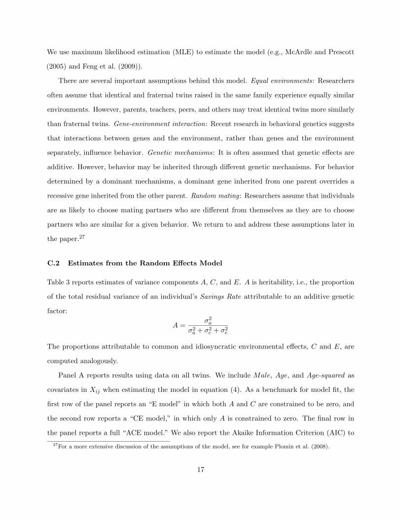
We use maximum likelihood estimation (MLE) to estimate the model (e.g., McArdle and Prescott

(2005) and Feng et al. (2009)).

There are several important assumptions behind this model. Equal environments: Researchers

often assume that identical and fraternal twins raised in the same family experience equally similar

environments. However, parents, teachers, peers, and others may treat identical twins more similarly

than fraternal twins. Gene-environment interaction: Recent research in behavioral genetics suggests

that interactions between genes and the environment, rather than genes and the environment

separately, influence behavior. Genetic mechanisms: It is often assumed that genetic effects are

additive. However, behavior may be inherited through different genetic mechanisms. For behavior

determined by a dominant mechanisms, a dominant gene inherited from one parent overrides a

recessive gene inherited from the other parent. Random mating : Researchers assume that individuals

are as likely to choose mating partners who are different from themselves as they are to choose

partners who are similar for a given behavior. We return to and address these assumptions later in

the paper.27

C.2 Estimates from the Random Effects Model

Table 3 reports estimates of variance components A, C, and E. A is heritability, i.e., the proportion

of the total residual variance of an individual’s Savings Rate attributable to an additive genetic

factor:

A =σ2a

σ2a + σ2c + σ2e

The proportions attributable to common and idiosyncratic environmental effects, C and E, are

computed analogously.

Panel A reports results using data on all twins. We include Male, Age, and Age-squared as

covariates in Xij when estimating the model in equation (4). As a benchmark for model fit, the

first row of the panel reports an “E model” in which both A and C are constrained to be zero, and

the second row reports a “CE model,” in which only A is constrained to zero. The final row in

the panel reports a full “ACE model.” We also report the Akaike Information Criterion (AIC) to

27For a more extensive discussion of the assumptions of the model, see for example Plomin et al. (2008).

17

compare fit across models and likelihood ratio (LR) statistics and p-values for comparing the “E

model” against the “CE model,” and the “CE model” against the “ACE model.”

We draw several conclusions from the analysis in the table. First, based on AIC, the full ACE

model is strongly preferred; based on the LR, the full ACE model is preferred over a CE model,

which in turn is preferred at the 1%-level over an E model. That is, empirically modeling a genetic

factor significantly improves the fit of a model which explains cross-sectional variation in individual

savings behavior. Second, we quantify the proportion of the total residual variation in savings

behavior attributable to a genetic effect A and find that it is 36 percent (statistically significant

at the 1%-level). That is, variation in savings behavior originates to a large extent from genetic

variation across individuals. This result is in contrast to our evidence regarding C, which is estimated

to zero, suggesting that savings behavior on average is not explained to any significant extent by

differences in the common parental environment in which children grow up. Finally, we find that

the idiosyncratic environment E contributes substantially to the variation in savings behavior. E is

64 percent, and is statistically significant at all levels. This is the largest component in the model,

but captures an entire set of possible individual-specific life experiences, shocks, other non-genetic

circumstances as well as measurement error. It suggests that life events influences an individual’s

savings behavior, such that experiences of certain shocks significantly change an individual’s savings

behavior.

In Panel B of the table, we reestimate the model in equation (4) for same sex twins only. In the

analysis in the previous panel we did control for gender through an indicator variable as a covariate

in Xij , but dropping opposite sex twins is an alternative approach, and one that is sometimes used

in behavioral genetics research. Excluding these individuals from our analysis does not significantly

change any of our conclusions. The A (E) component is still about 36 (64) percent.

Panel C reports results on gender-based genetic differences in savings behavior, i.e., we ask to

which extent genes influence savings differently for men and women. To answer this question, we

estimate separate models based on gender. We find that for men, the A component is 42 percent,

i.e., larger than for women, for whom it is only 29 percent. That is, the relative genetic variation

of men’s propensity to save is about 44 percent larger than that of women. The C component is

18

zero for men, but 2.4 percent for women, which is not statistically significant. Thus, there is some

evidence that while the savings behavior of men is more attributable to their genes, the behavior

of women in the savings domain is affected relatively more by individual-specific life experiences.

The behavior of an individual’s spouse can be one such life event which impacts behavior and is

captured by E in our model. A spouse effect is expected to be strongest for women from older age

cohorts, for which the spouse on average potentially influences savings behavior the most. There is

evidence supporting such predictions because the E component is very similar for younger men and

women, while it is 60 percent for older men compared to 77 percent for older women (untabulated).

What are the possible interpretations of our results? One interpretation of the significant genetic

component is that preferences for risk, time, and/or bequest are genetic, and that they in turn affect

savings behavior. It has already been documented by others that individuals who are more risk

averse also tend to save more (e.g., Lusardi (1998)), and risk aversion seems to have a significant

genetic component (e.g., Kuhnen and Chiao (2009), Barnea et al. (2010), and Cesarini et al. (2009b)).

To the extent that savings behavior reflects precautionary savings motives, our evidence can be

interpreted as genetic risk aversion affecting individuals’ savings propensities.

Another possible interpretation is that genetic time preferences are responsible for a genetic

component of savings behavior. In a standard economic model of savings behavior, individuals

who are more patient save more. Some researchers have recently made references to a “patience

gene” (Bernheim, 2009) such that those equipped with such genes would then be predicted to save

more. There is also emerging experimental evidence that individuals’ discounting of the future has

a genetic component (Eisenberg et al., 2007). Our evidence can thus be interpreted as individuals’

time preferences and patience having a genetic component which affects savings behavior among

individuals.

C.3 Parent-Child Social Transmission Effects for Subsets of Individuals

Another striking result so far is that parenting and the common family environment seem to affect

savings behavior very little, if at all. This is surprising given that social transmission of savings

behavior from parents to their children seems to be such a natural mechanism behind significant

19

parent-child similarities in behavior (e.g., Bisin and Verdier (2000); Bisin et al. (2004), Fernandez

et al. (2004), and Knudsen et al. (2006)). While the parenting effect on savings behavior is zero on

average, we examine in Table 4 the possibility that a significant effect emerges for specific subsets of

individuals.

We first examine different subsets of individuals based on their age. More specifically, in Panel A

of the table we estimate and report the variance components A, C, and E for separate age groups:

the youngest (Age ≤ 35), the oldest (50 < Age ≤ 65), as well as those of ages in-between. We find

that the total parental effect on children’s savings behavior, through genes as well as socialization,

i.e., A + C in the table, is the largest (46 percent) for the youngest in our sample, compared to

only 30 percent for the oldest. That is, parental effects on individuals’ savings behavior are most

significant earlier in life, subsequently decaying. The explanation for this decay is the disappearance

of the effect of social transmission from parents to their children, while the genetic effect does

not change significantly. In particular, we find that a significant C component emerges for the

youngest individuals in our sample. The common environment explains about 17 percent of the

cross-sectional variation in the propensity to save among the youngest. This result contrasts with

the C components for any of the other age groups, which are found to be zero.28

Our interpretation of this evidence is that parent-child social transmission does indeed affect

children’s savings behavior, but early on in life, and unlike genetic effects it does not seem to have life

long impact on individuals’ savings behavior. These results are consistent with work in behavioral

genetics which has documented a significant effect of the common family environment in early ages

on, e.g., personality, but also found that such effects approach zero in adulthood (e.g., Bouchard

(1998)). While our analysis in the previous section did not show any significant average effect of

the common family environment on savings behavior, our analysis by age groups reveals that the

parental environment seems to be relatively more important in explaining the savings behavior

of the youngest individuals. One possibility, which is open to future research, is that peer effect,

28We find that genes still explain as much as 30 percent of the cross-sectional variation in saving propensities amongthose older than 50 years of age. The persistence of behaviors with strong genetic origins is consistent with existingevidence; see, e.g., the work by McClearn et al. (1997) on a genetic component of cognitive ability among twins age 80or older (it has long been established that cognitive ability is genetic, but the new finding of this study is that thegenetic effect is so persistent).

20

relative to parent effects, become more important for savings behavior as individuals grow older.

We have also examined family characteristics related to the structure and the size of the family.29

More specifically, we predict that when parents have only a fixed supply of resources (e.g., time)

for socialization during which children may learn behaviors from their parents, then the presence

of non-twin siblings competing for such scarce parental resources may reduce the average effect

of parenting. That is, competition and constraints within the family may significantly reduce

parent-child influence through socialization, and thus affect savings behavior.

Panel B of Table 4 reports separate model estimates for twins who grew up in families with

no non-twin siblings compared to those who grew up with non-twin siblings. The common family

environment explains 15 percent of the cross-sectional variation in savings propensities among

individuals with no siblings. The effect is statistically significant at the 1%-level. Conversely, we

find no significant effect of parenting when there are non-twin siblings in the family in which the

twins grew up. That is, the presence of siblings seems to reduce the parent-child social transmission

effect on savings behavior.

The conclusion is that the particular structure or size of the family in which an individual grew

up can significantly influence savings behavior at a much later point in life. In particular, our results

suggest that within-family constraints and competition for scarce parental resources can significantly

influence the propensity to save in adulthood. By showing for which specific subsets of individuals

a parent-child social transmission effect emerges, these results provide further understanding of the

origins of individuals’ savings behavior.

C.4 Robustness

Table 5 presents several robustness checks with respect to our measure of savings behavior as well

as the equal environment assumption.

Preferences for Risk, Time, and Bequest. In a standard life cycle model, the savings behavior

of an individual will depend on age and in particular preferences with respect to risk, time, and

bequest. In Panel A, we control for a measure of revealed risk preferences, the relative equity share

29See Becker (1991) for important work on the family in economic research.

21

in an individual’s financial portfolio.30 We also include the number of children as a measure of

bequest motive. We find that the A, C, and E components are essentially unchanged when we

control for risk aversion and bequest. This result implies that differences in risk aversion or bequest

across individuals do not completely explain our finding of a genetic factor influencing savings

behavior, and is consistent with heritable time preferences.

Measuring Savings Behavior. The savings rate we have introduced above eliminates the unrealized

change in home value from the total change in net worth. Alternatively, and closely related to the

savings rate proposed by Dynan et al. (2004), we can add the change in home value to the disposable

income by which we scale the total change in net worth (Savings Rate 2 ). We also examine a

definition of the savings rate (Savings Rate 3 ) that simply relates the total unadjusted change in net

worth to the unadjusted disposable income. Panel B reports results for both alternative measures of

savings behavior.31 Our results do not seem sensitive to how we measure savings behavior.

Equal Environments. If identical twins are treated more similarly than fraternal twins, then our

model may attribute such unequal environments to the genetic component A. One approach to

this problem is to study twins separated soon after birth who were thus “reared apart.” C is by

construction zero for these twins as they did not share a common parental environment. However,

it is uncommon for adoption authorities to separate twins and with the additional filters we use

when constructing our data set, we end up with a sample that is too small for reliable statistical

analysis (2 identical and 40 fraternal twin pairs). However, most research on reared apart twins

confirms results from data sets that include twins who grew up in the same family; see, e.g., the

seminal work by Bouchard et al. (1990) and more recent work in financial economics by Barnea et al.

(2010). Unfortunately, our data set contains too few twins that were reared apart. As an alternative

robustness check we study twins who do not interact or who interact little with each other as adults,

measured through survey questions by the STR (“How often do you have contact?”). Panel C of

Table 5 estimates and reports the variance components A, C, and E for separate contact intensity

30To not confound risk preferences with factors affecting stock market participation, we only include stock marketparticipants. Accordingly the sample size drops to 12,616 twins.

31Note that in the construction of Savings Rate 2 and Savings Rate 3, we have again dropped the top and bottomone percentile of the respective distributions. Therefore, the number of observations is slightly smaller than theprevious sample of 17,630.

22

groups. We find a significant genetic component of savings behavior even among those who have no

or little contact, reducing concerns that genetic and common environmental effects were confounded

in our previous analysis.32

Genetic Mechanisms. Our analysis so far has assumed an additive genetic effect. For some

behaviors, geneticists have found evidence of a dominant genetic effect. A dominant genetic effect

can be added to the model in equation (4); see, e.g., Plomin et al. (2008) for details. Our estimate

of a dominant genetic component D is 8 percent, albeit not statistically significant at conventional

levels, and the total genetic component (A+D) from this model is 37 percent (untabulated). That

is, our conclusions of a significant genetic effect on the propensity to save does not change when

empirically modeling a dominant gene effect.

Random Mating. Our empirical approach assumes that individuals mate randomly, at least

relative to the particular behavior examined in the study. If, however, individuals tend to choose

mates like themselves, then fraternal twins share more than 50 percent of their genes, and thus more

similarities on genetic behavior, because they receive similar genes from their fathers and mothers.

There is some research in sociology which suggests that positive assortative mating by culture is

more important than positive assortative mating by economic behavior (Kalmijn, 1994), but we

are not aware of work on mating specifically based on savings propensities.33 It is important to

emphasize, however, that positive assortative mating would downward bias our reported estimates

of the A component, as it would create more similarity between fraternal twins.

V Gene-Environment Interactions

Neurobiologists have demonstrated that the expression of genes can change in response to certain

experiences or exposure to particular environments (Rutter (2006)). Such gene-environment (GxE)

32We also find that a significant C component (22 percent) emerges among those who interact a lot. Those infrequent contact create their own common environment as they communicate after separating from their parents. Thisresult is consistent with social interaction affecting individuals’ behavior through for example word-of-mouth (e.g.,Bikhchandani et al. (1992, 1998)), and emphasizes the importance of social transmission of behavior from others thanparent.

33Economists and sociologists have examined assortative mating based on education (e.g., Pencavel (1998) andMare (1991)) and the extent to which which individuals marry to diversify their labor income risk versus marry forlove (Hess, 2004).

23

interaction can also change the relative importance of genetic factors as genes are moderated by

environmental factors. While an individual’s genes might provide an innate predisposition to a

certain behavior, specific environmental conditions determine the extent to which this potential

will indeed be realized. As reviewed above, there is some recently emerging work on the genetic

origins of economic behaviors, but so far there is little work on gene-environment interactions. In

this section, we discuss existing research related to gene-environment interplay. We then empirically

analyze such interaction effects with respect to savings behavior.34

Two theoretical models of GxE interactions offer competing predictions for GxE interaction

effects. First, the bioecological model, proposed by Bronfenbrenner and Ceci (1994), suggests that

genetic influences on behavior are most evident when the environment is supportive, because of a

predicted greater actualization of genetic predispositions in supportive compared to less supportive

environments.35 This model can, for example, explain the evidence in Taylor et al. (2010), who

examine the GxE interaction between genetic ability to read and teacher quality, and show that

the genetic effect on reading fluency among first- and second-graders increases as the quality of

the children’s teacher increases (measured by reading gain among non-twin classmates). Second,

the diathesis-stress model suggests that heritability of a behavior should be greater in poorer

environments, where stressors may lead to the expression of genes that would not be actualized in

more supportive environments. This model has, for example, recently been proposed to explain

why some behavioral disorders have a greater relation with specific genes in environments where

individuals have been exposed to a large number of stressful life events (e.g., Caspi et al. (2002) and

Caspi et al. (2003)).

Conceptually, we can distinguish between moderating environments that are obligatorily shared

by both twins and those that are specific to an individual twin. As Purcell (2002) points out,

the former, if unmodeled, will induce an upward bias of A, the latter type of gene-environment

interaction on the other hand will bias E upwards. We start our analysis of gene-environment

34In a recent paper on the development of abilities in young individuals, Cunha and Heckman (2010) summarize thearguments well by arguing that “Additive “nature” and “nurture” models, while standard and still used in manystudies of heritability and family influence, mischaracterize how ability is manifested. Abilities are produced, and geneexpression is governed, by environmental conditions.” (p.3)

35Economists may use a different terminology to describe “supportive environments,” such as environments withmore individual opportunities or choice, or less constraining environments.

24

interactions with the parental environment both twins experienced. We then examine the importance

of twin-specific environments.36

A Early Environment

We examine the extent to which potentially important characteristics of the parental and family

environment in childhood and early adolescence interact with genetic effects. One characteristic

of an individual’s early environment is the socioeconomic status (SES) of the family in which the

individual grew up. Parental education is our measure of family SES (and related environmental

factors), and we are able to separate between those whose parents have no college education and

those with parents with at least college education.37

Panel A of Table 6 reports that the genetic influence on an individual’s savings behavior is

stronger among those who grew up in high-SES families. We find that genes explain 39 percent

of the cross-sectional variation in savings propensity among individuals who grew up in high-SES

families. For those who grew up in low-SES families, the corresponding A component is only 32

percent. That is, early environmental factors in an individual’s life seem to result in different genetic

expression of savings behavior much later in life.

We conclude that the socioeconomic status of an individual’s family in childhood or early

adolescence is a moderator for genetic influences on savings behavior much later in life, and thus

governs the extent to which an innate predisposition to a behavior will be actualized. This evidence

is supportive of the bioecological model of GxE interactions. A less constraining environment, at

least in the sense of higher socioeconomic status of the family in which an individual grew up, is

related to a stronger genetic expression in the domain of savings behavior. Of course, this result

opens for a series of currently unanswered research questions about the exact nature of the genetic

36In addition to gene-environment interactions, twins (or their parents) might have selected into certain environments,reflecting gene-environment correlations. Correlation between genes and the shared environment will bias C upwards,while correlation between genes and the individual-specific environment will bias A upwards. The effects of gene-environment correlations are hence the opposite of the effects of gene-environment interactions. See Purcell (2002) fordetails. The current analysis abstracts from gene-environment correlations.

37Parents’ education is admittedly an imperfect measure of SES, but we are not able to measure, e.g., parents’wealth during the period their children grew up. While imperfect, parental education is a measure that has been usedby other researchers, and we do not believe that possible measurement error in this measure causes any systematicbiases in our empirical analysis.

25

and environmental influences on savings behavior that are related to a family’s socioeconomic status.

B Later Environment

We also examine whether an individual’s current environment (as opposed to the environment the

individual grew up in) interacts with genetic effects. There are several environmental factors which

we predict to be potentially important for the genetic expression of savings behavior. We report

these results related to an interplay with “later environments” in Panels B and C of Table 6.

We first examine the importance of an individual’s own wealth. Wealthier individuals are, on

average, less constrained and thus more likely to behave as predicted by their innate predisposition.

For example, a poor individual in our sample may be constrained from saving, regardless of how risk

averse or patient the individual is. In contrast, a wealthy individual has the choice of whether to save

or to spend. Panel B of the table reports that genes explain about 18 percent of the cross-sectional

variation of the propensity to save among the poorest individuals, meaning those in the lowest

quintile of the wealth distribution. This may be compared to 39 percent, i.e., more than double,

among the wealthiest individuals, i.e. those in the highest quintile of the wealth distribution. That

is, the genetic effect on savings behavior is much stronger among the wealthy compared to the

relatively poor. In other words, the savings behavior of the poorest individuals originates more

from individual-specific life experiences. This evidence is consistent with wealthy individuals being

less constrained resulting in greater actualization of genetic predispositions of savings behavior.

This evidence shows that genetic effects can de facto be censored when an individual is subject to

constraining environments.

An alternative is to examine an individual’s current socioeconomic status rather than wealth,

though wealth is of course a measure of SES. Using education as a measure of SES, we find that the

genetic effect if larger for high-SES individuals compared to low-SES individuals, consistent with

the wealth result. The A component is 23 percent for low-SES individuals compared to 35 percent

for high-SES individuals (untabulated). This result also shows that the current socioeconomic

environment is a stronger moderator (by more than 50 percent) of genetic effects on savings

behavior compared to the parental and family environment in childhood and early adolescence. Most

26

importantly, a less constraining individual socioeconomic environment with more opportunities,

both early and later in life, amplifies the genetic expression of savings behavior.

Another potentially important environmental factor is the community/region where an individual

lives. One such environmental characteristic is the population density of an area, because of

the potential for significant differences in, e.g., social interaction with peers and consumption

choices. Using data from Statistics Sweden, we classify regions into very rural (the first quintile

of the corresponding density distribution), very urban (the top quintile of the distribution), and

intermediate. The average number of individuals per square kilometer in very rural areas such as

Lapland is 12, compared to 2,162 for very urban areas such as the city of Stockholm. Panel C reports

that the genetic component, A, is 56 percent in sparsely-populated rural areas, i.e., almost double

the effect in more densely populated areas, where it is only 32 percent. That is, an individual’s

genetic predisposition is found to be expressed significantly more strongly among individuals in

rural communities. One interpretation of this evidence is that urban life may result in exposure

to more idiosyncratic life experiences, through social interaction with peers who also live there or

through some other mechanisms, which may affect the importance of the genetic effect on savings

behavior. That is, in urban environments, an individual’s savings propensity may be governed more

by the environment such as peers and social networks.

The conclusion from the evidence reported in this section is that gene-environment interplay is

important in explaining the origins of savings behavior. That is, an individual’s innate predisposition

is actualized to a greater or lesser extent depending on the environment that the individual

experiences, and we found that both the earlier and later environments in life act as moderators of

genetic effects. Of course, these results opens for a series of currently unanswered research questions

about the exact nature of the genetic and environmental influences on savings behavior, and what

other environmental factors are potentially important moderators for genetic influence on savings

behavior.

27

VI What the Evidence Does and Does Not Mean

In this section, we discuss several important implications of our findings.

Implications for Accumulation of Wealth

The findings in this paper, taken together with the existing evidence on genetic determinants of

income and asset allocation (Behrman and Taubman (1989), Taubman (1976), and Barnea et al.

(2010)), suggest that cross-sectional variation in wealth, in particular at retirement age, should

to some extent reflect genetic differences across individuals. In Table 7, we estimate model (4)

for the wealth of all individuals that are around retirement age (60 to 69), that is we study the

outcome of many years of savings and investment behavior.38 We find that about 38 percent of

the cross-sectional variation in wealth accumulated up to retirement is explained by genetic factors.

The effect of the common family environment, which by model construction reflects wealth inherited

from parents, explain seven percent of the cross-sectional variation.39 The remaining 55 percent is

due to individual-specific life experiences.

Behavioral Factors

So far in the paper, we have taken the perspective that an individual’s savings behavior is mainly

determined by preferences, i.e., we have considered a standard economic model of savings behav-

ior. However, our evidence does not mean that these are the only candidate explanations. Some

economists have argued that non-standard models and “behavioral factors” are also important

explanations for variation in savings (or the lack of savings) across individuals; see, e.g., Bernheim

et al. (2000) and Madrian and Shea (2001). It is, for example, possible that biases such as lack of

self-control results in insufficient savings among some individuals (e.g., Thaler and Shefrin (1981)).40

It would be very interesting to study the extent to which retirement savings biases are innate. The

38Differently from our main sample, we include all individuals that in 2006 were between 60 and 69 years old andhad non-missing wealth data between 2003 and 2006. To avoid that our results are affected by outliers, we dropindividuals in the bottom and top one percent of the distribution.

39While this effect is consistent with parent-child social transmission of behavior on average playing only a limitedrole for savings and asset allocation choices, it is lower than some estimates for the U.S. (e.g., Davies and Shorrocks(2000)). This difference is likely due to our subset of older individuals.

40See Benartzi and Thaler (2007) for a review of biases in retirement savings behavior.

28

evidence that lack of self-control, at least extreme versions such as attention-deficit hyperactivity

disorder (ADHD), has a genetic component (Barkley, 1997) certainly suggests that biases affecting

an individual’s savings behavior may be partially genetic.

Variation Across Time and Countries

While we find that genes explain about 35 percent of the variation in savings behavior across

individuals in our sample, it is important to emphasize that this is not a universal biological

constant, but an estimate relative to the amount of environmental variation in the sample. If there

is limited variation in environmental factors, then the genetic component will indeed be relatively

large. Our data are from Sweden, a country which is often perceived to have relatively high cultural

homogeneity (meaning low variation in environmental factors in the context of our model). Since

we only observe individuals from one country at one point in time, our empirical analysis cannot

capture the relative importance of country characteristics such as culture, i.e., we can not measure

whether changes in a country’s “savings culture” at large affect individual behavior. Finally, the

focus on one country rather than a broader set, likely reduces the amount of total variation in

environmental factors.

Oblique Socialization and Peer Effects

Our evidence should not be interpreted as meaning that peer and social networking effects are not

important for savings behavior.41 First, while one specific social transmission mechanism — the one

between parents and their children — is found to be small, our research also reveals some of the

specific subsets of individuals for which parent-child transmission of behavior are significant. Second,

in this paper we have not analyzed peers effects and their effects on individuals’ savings behavior.

However, one result in our paper which indeed suggests that social interaction is important is our

twin-twin communication evidence: Twins who interact more with each other have more similar

savings behavior. This result is consistent with social interaction affecting individuals’ behavior

in the financial domain (e.g., Bikhchandani et al. (1992, 1998), Shiller (1995), and Hirshleifer

41Several studies in economics and finance suggest that peer effects are important in the financial domain (e.g.,Madrian and Shea (2000), Hong et al. (2004), and Brown et al. (2008)).

29

and Teoh (2009)) and emphasizes the potential importance of “oblique socialization” (Cavalli-

Sforza and Feldman, 1981). To the extent that twins have non-overlapping social networks, peer

effect on savings will in our paper be captured by the individual idiosyncratic factor (E in our model).

Effectiveness of Public Policy

Economists and policy makers have recently devoted significant effort to examining financial literacy

and methods to change individual savings behavior (e.g., Thaler and Benartzi (2004), Lusardi

and Mitchell (2009), and Bayer et al. (2009)). Our evidence does not mean that public policy

and financial literacy education in the domain of savings behavior can never be effective. It is

correct, as argued by Bernheim (2009), that evidence of a genetic component of savings behavior has

implications for economists’ evaluations of the sensitivity of savings behavior to policy initiatives:

Environmental factors are presumably more amenable to policy than innate predispositions. But

some public policy can affect the average amount of savings without affecting the variation across

individuals. For example, policy that changes a country’s “savings culture” are not captured in our

model. Moreover, educational experiences may be individual-specific and would be reflected in the

idiosyncratic environmental component, which explains well over 50 percent of the cross-sectional

variation in savings behavior in all our analysis. We also find evidence of significant gene-environment

interplay, which opens the question of whether policy initiatives interact with genetic factors, so

that some individuals are more susceptible to policy than others. In this sense, understanding the

genetic component of savings behavior and its interactions with the environment may produce more

effective policies.

VII Conclusion

The goal of this study has been to examine the origins of individuals’ savings behavior. That is, what

makes an individual a “spender” while another individual, with similar observable characteristics,

saves a large proportion of his or her income? Our work suggests that there is not a simple answer

to this fundamental economics question. By contrast, an individual’s savings behavior is governed

by both innate genetic predispositions, social transmission of behavior from parents to their children,

30

and gene-environment interplay where the environment moderates genetic influences. Genes explain

on average about 35 percent of the variation in savings rates across individuals, but the genetic

expression of savings behavior is stronger in environments characterized by higher socioeconomic

status (own or parental). We find no evidence that parenting matters on average for savings behavior,

but a significant effect of parent-child socialization does emerge when studying young individuals,

and those who grew up in environments characterized by less competition for parental resources.

Individual-specific experiences turn out to be a very important explanation for behavior in the

savings domain, and most intensely so in urban communities, raising the question of which specific

life events are most important for an individual’s propensity to save. We also discussed what the

reported evidence may mean for public policy aimed at changing individual savings behavior.

31

References

Ashenfelter, O., Krueger, A. B., 1994. Estimates of the economic returns to schooling from a newsample of twins. American Economic Review 84 (5), 1157–1173.

Ashenfelter, O., Rouse, C., 1998. Income, schooling, and ability: Evidence from a new sample ofidentical twins. Quarterly Journal of Economics 113 (1), 253–284.

Barkley, R. A., 1997. ADHD and the nature of self-control. Guilford Press, New York, NY.

Barnea, A., Cronqvist, H., Siegel, S., 2010. Nature or nurture: What determines investor behavior?Forthcoming Journal of Financial Economics.

Barsky, R. B., Juster, F. T., Kimball, M. S., Shapiro, M. D., 1997. Preference parameters andbehavioral heterogeneity: An experimental approach in the health and retirement study. QuarterlyJournal of Economics 112, 537–579.

Bayer, P. J., Bernheim, B. D., Scholz, J. K., 2009. The effects of financial education in the workplace:Evidence from a survey of employers. Economic Inquiry 47, 605–624.

Becker, G., Tomes, N., 1976. Child endowments and the quantity and quality of children. Journal ofPolitical Economy 84 (4), 143–162.

Becker, G. S., 1976. Altruism, egoism, and genetic fitness: Economics and sociobiology. Journal ofEconomic Literature 14, 817–826.

Becker, G. S., 1991. A treatise on the family. Harvard University Press, Cambridge, MA.

Behrman, J., Taubman, P., 1989. Is schooling mostly in the genes? Nature-nurture decompositionusing data on relatives. Journal of Political Economy 97, 1425–1446.

Behrman, J. R., Taubman, P., 1976. Intergenerational transmission of income and wealth. AmericanEconomic Review 66, 436–440.

Benartzi, S., Thaler, R. H., 2007. Heuristics and biases in retirement savings behavior. Journal ofEconomic Perspectives 21, 81–104(24).

Benjamin, D., Chabris, C., Glaeser, E., Gudnason, V., Harris, T., Laibson, D., Launer, L., Purcell,S., 2008. Genoeconomics. The National Academies Press, Ch. 15, pp. 304–335.

Bernheim, B., 2009. On the potential of neuroeconomics: A critical (but hopeful) appraisal. AmericanEconomic Journal: Microeconomics 1 (2), 1–41.

Bernheim, B., Shleifer, A., Summers, L., 1985. The strategic bequest motive. Journal of PoliticalEconomy, 1045–1076.

Bernheim, B. D., Forni, L., Gokhale, J., Kotlikoff, L. J., 2000. How much should Americans besaving for retirement? American Economic Review 90 (2), 288–292.

Bernheim, B. D., Garrett, D. M., 2003. The effects of financial education in the workplace: Evidencefrom a survey of households. Journal of Public Economics 87, 1487–1519.

32

Bernheim, B. D., Garrett, D. M., Maki, D. M., 2001. Education and saving: The long-term effectsof high school financial curriculum mandates. Journal of Public Economics 80, 435–465.

Bikhchandani, S., Hirshleifer, D., Welch, I., 1992. A theory of fads, fashion, custom, and culturalchange as informational cascades. Journal of Political Economy 100 (5), 992–1026.

Bikhchandani, S., Hirshleifer, D., Welch, I., 1998. Learning from the behavior of others: Conformity,fads, and informational cascades. Journal of Economic Perspective 12 (3), 151–170.

Bisin, A., Topa, G., Verdier, T., 2004. Religious intermarriage and socialization in the United States.Journal of Political Economy 112 (3), 615–664.

Bisin, A., Verdier, T., 2000. Beyond the melting pot: Cultural transmission, marriage, and theevolution of ethnic and religious traits. Quarterly Journal of Economics 115 (3), 955–988.

Bisin, A., Verdier, T., 2001. The economics of cultural transmission and the dynamics of preferences.Journal of Economic Theory 97 (2), 298 – 319.

Bisin, A., Verdier, T., 2008. Cultural transmission. In: Durlauf, S. N., Blume, L. E. (Eds.), TheNew Palgrave Dictionary of Economics. Palgrave Macmillan, Basingstoke.

Bjorklund, A., Lindahl, M., Plug, E., 2006. The origins of intergenerational associations: Lessonsfrom Swedish adoption data. Quarterly Journal of Economics 121, 999–1028.

Black, S. E., Devereux, P. J., Salvanes, K. G., 2005. Why the apple doesn’t fall far: Understandingintergenerational transmission of human capital. American Economic Review 95 (1), 437–449.

Borjas, G. J., 1992. Ethnic capital and intergenerational mobility. Quarterly Journal of Economics107 (1), 123–150.

Bouchard, T. J., 1998. Genetic and environmental influences on adult intelligence and special mentalabilities. Human Biology 70, 257–279.

Bouchard, T. J., Lykken, D. T., McGue, M., Segal, N. L., Tellegen, A., 1990. Sources of humanpsychological differences: The Minnesota study of twins reared apart. Science 250, 223–228.

Bowles, S., Gintis, H., 2002. The inheritance of inequality. Journal of Economic Perspectives 16 (3),3–30.

Boyd, R., Richerson, P., 1985. Culture and the Evolutionary Process. University of Chicago Press,Chicago, IL.

Brennan, T. J., Lo, A. W., 2009. The origin of behavior. Working Paper, MIT Sloan School ofManagement.

Bronfenbrenner, U., Ceci, S. J., 1994. Nature-nurture in developmental perspective: A bioecologicaltheory. Psychological Review 101, 568–586.

Brown, J. R., Ivkovic, Z., Smith, P. A., Weisbenner, S., 2008. Neighbors matter: Causal communityeffects and stock market participation. Journal of Finance 63, 1509–1532.

33

Browning, M., Lusardi, A., 1996. Household saving: Micro theories and micro facts. Journal ofEconomic Literature 34, 1797–1855.

Calvet, L. E., Campbell, J. Y., Sodini, P., 2007. Down or out: Assessing the welfare costs ofhousehold investment mistakes. Journal of Political Economy 115, 707–747.

Calvet, L. E., Campbell, J. Y., Sodini, P., 2009. Fight of flight? Portfolio rebalancing by individualinvestors. Quarterly Journal of Economics 124, 301–348.

Camerer, C., Loewenstein, G., Prelec, D., 2005. Neouroeconomics: How neuroscience can informeconomics. Journal of Economic Literature 43, 9–64.

Caplin, A., Dean, M., 05 2008. Dopamine, reward prediction error, and economics. Quarterly Journalof Economics 123 (2), 663–701.

Carpenter, J. P., Garcia, J. R., Lum, J. K., 2009. Can dopamine receptor genes explain economicpreferences and outcomes? Working Paper, Middlebury College.

Carroll, C. D., 1992. The buffer-stock theory of saving: Some macroeconomic evidence. BrookingsPapers on Economic Activity 23 (1992-2), 61–156.

Carroll, C. D., Samwick, A., 1998. How important is precautionary saving. Review of Economicsand Statistics 80 (No. 3), 410–419.

Carroll, C. D., Samwick, A. A., 1997. The nature of precautionary wealth. Journal of MonetaryEconomics 40 (1), 41–71.

Caspi, A., McClay, J., Moffitt, T., Mill, J., Martin, J., Craig, I., Taylor, A., Poulton, R., 2002. Roleof genotype in the cycle of violence in maltreated children. Science 297 (5582), 851.

Caspi, A., Sugden, K., Moffitt, T. E., Taylor, A., Craig, I. W., Harrington, H., McClay, J., Mill, J.,Martin, J., Braithwaite, A., Poulton, R., 2003. Influence of life stress on depression: moderationby a polymorphism in the 5-HTT gene. Science 301 (5631), 386–389.

Cavalli-Sforza, L., Feldman, M., 1981. Cultural Transmission and Evolution: A QuantitativeApproach. Princeton University Press, Princeton, NJ.

Cesarini, D., Dawes, C. T., Johannesson, M., Lichtenstein, P., Wallace, B., 2009a. Genetic variationin preferences for giving and risk taking. Quarterly Journal of Economics 124, 809–842.

Cesarini, D., Johannesson, M., Lichtenstein, P., Sandewall, O., Wallace, B., 2009b. Genetic variationin financial decision making. Forthcoming Journal of Finance.

Charles, K. K., Hurst, E., 2003. The correlation of wealth across generations. Journal of PoliticalEconomy 111, 1155–1182.

Chiteji, N. S., Stafford, F. P., 1999. Portfolio choices of parents and their children as young adults:Asset accumulation by African-Americans. American Economic Review 89, 377–380.

Cunha, F., Heckman, J. J., 2010. Investing in our young people. Working Paper, University ofChicago, Department of Economics.

34

Davies, J. B., Shorrocks, A. F., 2000. The distribution of wealth. In: Atkinson, A. B., Bourguignon,F. (Eds.), Handbook of Income Distribution. Elsevier, Ch. 11, pp. 605–675.

Deaton, A., 1991. Saving and liquidity constraints. Econometrica 59 (5), 1221–1248.

Dohmen, T., Falk, A., Huffman, D., Sunde, U., 2008. The intergenerational transmission of risk andtrust attitudes. Working Paper, Institute for the Study of Labor (IZA).

Donkers, B., Melenberg, B., Van Soest, A., 2001. Estimating risk attitudes using lotteries: A largesample approach. Journal of Risk and Uncertainty 22 (2), 165–195.

Dreber, A., Apicella, C. L., Eisenberg, D. T. A., Garcia, J. R., Zamore, R. S., 2009. The 7Rpolymorphism in the dopamine receptor D4 gene (DRD4) is associated with financial risk-takingin men. Evolution and Human Behavior 30, 85–92.

Dreber, A., Rand, D. G., Garcia, J. R., Wernerfelt, N., Lum, J. K., Zeckhauser, R., 2010. Dopamineand risk preferences in different domains. Working Paper, Harvard University, John F. KennedySchool of Government.

Dynan, K. E., Skinner, J., Zeldes, S. P., 2004. Do the rich save more? Journal of Political Economy112 (2), 397–444.

Eisenberg, D., MacKillop, J., Modi, M., Beauchemin, J., Dang, D., Lisman, S., Lum, J., Wilson, D.,2007. Examining impulsivity as an endophenotype using a behavioral approach: a DRD2 taqi aand DRD4 48-bp VNTR association study. Behavioral and Brain Functions 3 (1), 2.

Feng, R., Zhou, G., Zhang, M., Zhang, H., 2009. Analysis of twin data using sas. Biometrics 65,584–589.

Fernandez, R., Fogli, A., Olivetti, C., 2004. Mothers and sons: preference formation and femalelabor force dynamics. Quarterly Journal of Economics 119 (4), 1249–1299.

Friedman, M., 1953. Choice, chance, and the personal distribution of income. Journal of PoliticalEconomy 61 (4), 277–290.

Fuchs, V. R., 1982. Self-employment and labor force participation of older males. Journal of HumanResources 17 (3), 339–357.

Guell, M., Rodrıguez Mora, J. V., Telmer, C., 2007. Intergenerational mobility and the informativecontent of surnames. Working Paper, Carnegie Mellon University, Tepper School of Business.

Harris, J. R., 1995. Where is the child’s environment? a group socialization theory of development.Psychological Review 102 (3), 458 – 489.

Harrison, G. W., Lau, M. I., Williams, M. B., 2002. Estimating individual discount rates in Denmark:A field experiment. American Economic Review 92 (5), 1606–1617.

Hess, G., 2004. Marriage and consumption insurance: What’s love got to do with it? Journal ofPolitical Economy 112 (2), 290–318.

35

Hirshleifer, D., Teoh, S. H., 2009. Thought and behavior contagion in capital markets. In: Hens, T.,Schenk-Hoppe, K. (Eds.), Handbook of Financial Markets: Dynamics And Evolution, Handbooksin Finance. North-Holland, Amsterdam, The Netherlands, Ch. 1, pp. 1–46.

Hirshleifer, J., 1977. Economics from a biological viewpoint. Journal of Law and Economics 20,1–52.

Hong, H., Kubik, J. D., Stein, J. C., 2004. Social interaction and stock-market participation. Journalof Finance 59 (1), 137–163.

Hubbard, R., Skinner, J., Zeldes, S., 1994. The importance of precautionary motives in explainingindividual and aggregate saving. In: Carnegie-Rochester Conference Series on Public Policy.Vol. 40. pp. 59–125.

Hubbard, R., Skinner, J., Zeldes, S., 1995. Precautionary saving and social insurance. Journal ofPolitical Economy, 360–399.

Kalmijn, M., 1994. Assortative mating by cultural and economic occupational status. AmericanJournal of Sociology 100 (2), 422.

Kimball, M., 1990. Precautionary saving in the small and in the large. Econometrica 58 (1), 53–73.

Kimball, M. S., Sahm, C. R., Shapiro, M. D., 2009. Risk preferences in the psid: Individualimputations and family covariation. American Economic Review 99 (2), 363–68.

Knowles, J., Postlewaite, A., 2004. Do children learn to save from their parents. Working Paper,University of Pennsylvania, Department of Economics.

Knudsen, E. I., Heckman, J. J., Cameron, J. L., Shonkoff, J. P., 2006. Economic, neurobiological,and behavioral perspectives on building Americas future workforce. Proceedings of the NationalAcademy of Sciences 103 (27), 10155–10162.

Kuhnen, C. M., Chiao, J., 2009. Genetic determinants of financial risk taking. PLoS ONE 4.

Leland, H., 1968. Saving and uncertainty: The precautionary demand for saving. Quarterly Journalof Economics 82 (3), 465–473.

Lichtenstein, P., Sullivan, P. F., Cnattingius, S., Gatz, M., Johansson, S., Carlstrom, E., Bjork, C.,Svartengren, M., Wolk, A., Klareskog, L., de Faire, U., Schalling, M., Palmgren, J., Pedersen,N. L., 2006. The Swedish twin registry in the third millennium: An update. Twin Research andHuman Genetics 9, 875–882.

Lusardi, A., 1998. On the importance of the precautionary saving motive. American EconomicReview 88 (2), 449–453.

Lusardi, A., 2001. Explaining why so many people do not save. Working Paper, Dartmouth College,Department of Economics.

Lusardi, A., Mitchell, O. S., 2009. How ordinary consumers make complex economic decisions:Financial literacy and retirement readiness. Working Paper, Dartmouth College, Department ofEconomics.

36

Maccoby, E. E., 2000. Parenting and its effects on children: On reading and misreading behaviorgenetics. Annual Review of Psychology 51 (1), 1–27.

Madrian, B. C., Shea, D., 2000. Peer effects and savings behavior in employer-sponsored savingsplans. Working Paper, University of Chicago, Graduate School of Business.

Madrian, B. C., Shea, D. F., 2001. The power of suggestion: Inertia in 401(k) participation andsavings behavior. Quarterly Journal of Economics 116, 1149–1525.

Mare, R. D., 1991. Five decades of educational assortative mating. American Sociological Review56, 15–32.

Marshall, A., 1920. Principles of Economics. Macmillan, London, U.K.

McArdle, J. J., Prescott, C. A., 2005. Mixed effects variance components models for biometricfamily analysis. Behavior Genetics 35, 631–652.

McClearn, G. E., Johansson, B., Berg, S., Pedersen, N. L., Ahern, F., Petrill, S. A., Plomin, R.,1997. Substantial genetic influence of cognitive abilities in twins 80 or more years old. Science276, 1560–1563.

Mischel, W., Shoda, Y., Rodriguez, M., 1989. Delay of gratification in children. Science 244 (4907),933–938.

Modigliani, F., Brumberg, R., 1954. Utility analysis and the consumption function: an interpretationof cross-section data. In: Kurihara, K. K. (Ed.), Post-Keynesian Economics. Rutgers UniversityPress, New Brunswick, NJ.

Mulligan, C., 1999. Galton versus the human capital approach to inheritance. Journal of PoliticalEconomy 107 (S6), S184–S224.

Netzer, N., 2009. Evolution of time preferences and attitudes toward risk. American EconomicReview 99, 937–955.

Pencavel, J., 1998. Assortative mating by schooling and the work behavior of wives and husbands.American Economic Review 88, 326–329.

Plomin, R., Defries, J. C., McClearn, G. E., McGuffin, P., 2008. Behavioral Genetics. WorthPublishers, New York, NY.

Reuben, E., Sapienza, P., Zingales, L., 2010. Time discounting for primary and monetary rewards.Economics Letters 106 (2), 125 – 127.

Richerson, P., Boyd, R., 2005. Not By Genes Alone. University of Chicago Press, Chicago, IL.

Robson, A. J., 1996. The evolution of attitudes to risk: Lottery tickets and relative wealth. Gamesand Economic Behavior 14, 190–207.

Robson, A. J., 2001. Why would nature give individuals utility functions? Journal of PoliticalEconomy 109, 900–914.

37

Robson, A. J., Samuelson, L., 2009. The evolution of time preference with aggregate uncertainty.American Economic Review 99 (5), 1925–53.

Rodgers, J. L., Kohler, H.-P., Kyvik, K. O., Christensen, K., 2001. Behavior genetic modeling ofhuman fertility: Findings from a contemporary danish twin study. Demography 38 (1), 29–42.

Rogers, A. R., 1994. Evolution of time preference by natural selection. American Economic Review84 (3), 460–81.

Rushton, J., Fulker, D. W., Neale, M. C., Nias, D. K., Eysenck, H. J., 1986. Altruism andaggression: The heritability of individual differences. Journal of Personality and Social Psychology50, 1192–1198.

Rutter, M., 2006. Genes and behavior: Nature/nurture interplay explained. Blackwell Publishers,Oxford, UK.

Sacerdote, B., 2002. The nature and nurture of economic outcomes. American Economic Review 92,344–348.

Sahm, C., 2007. How much does risk tolerance change? Working Paper, Federal Reserve Board.

Sapienza, P., Zingales, L., Maestripieri, D., 2009. Gender differences in financial risk aversion andcareer choices are affected by testosterone. Proceedings of the National Academy of Sciences106 (36), 15268–15273.

Shiller, R. J., 1995. Conversation, information, and herd behavior. American Economic Review85 (2), 181–185.

Skinner, J., 1988. Risky income, life cycle consumption, and precautionary savings. Journal ofMonetary Economics 22 (2), 237–255.

Solon, G., 1992. Intergenerational income mobility in the United States. American Economic Review82 (3), 393–408.

Taubman, P., 1976. The determinants of earnings: Genetics, family, and other environments: Astudy of white male twins. American Economic Review 66 (5), 858–870.

Taylor, J., Roehrig, A. D., Hensler, B. S., Connor, C. M., Schatschneider, C., 2010. Teacher QualityModerates the Genetic Effects on Early Reading. Science 328 (5977), 512–514.

Thaler, R. H., Benartzi, S., 2004. Save more tomorrow: Using behavioral economics to increaseemployee savings. Journal of Political Economy 112, 164–187.

Thaler, R. H., Shefrin, H. M., 1981. An economic theory of self-control. Journal of Political Economy89 (2), 392–406, english.

Venti, S. F., Wise, D. A., 1998. The cause of wealth dispersion at retirement: Choice or chance?American Economic Review 88 (2), 185–191.

Venti, S. F., Wise, D. A., 2000. Choice, chance, and wealth dispersion at retirement. Working Paper,National Bureau of Economic Research.

38

Wade, N., 2010. A decade later, genetic map yields few new cures. New York Times June 13, 2010,A1.

Warner, J. T., Pleeter, S., 2001. The personal discount rate: Evidence from military downsizingprograms. American Economic Review 91 (1), 33–53.

Zhong, S., Israel, S., Xue, H., Ebstein, R. P., Chew, S. H., 2009. Monoamine Oxidase A gene(MAOA) associated with attitude towards longshot risks. PLoS ONE 4.

Zyphur, M. J., Narayanan, J., Arvey, R. D., Alexander, G. J., 2009. The genetics of economic riskpreferences. Journal of Behavioral Decision Making 22, 367–377.

39

Table 1Summary Statistics

Panel A: Number of Twins by Zygosity and Gender

All Twins

Male Female TotalSame Sex:

MaleSame Sex:

FemaleOpposite

Sex Total

Number of twins (N ) 17,630 2,244 2,898 5,142 2,466 3,178 6,844 12,488

Fraction (%) 100% 13% 16% 29% 14% 18% 39% 71%

Panel B: Socio-demographic Characteristics

All TwinsVariable N Mean Median Std. Dev. Mean Median Std. Dev.

Age 17,630 48.96 52.00 12.36 53.23 55.00 9.70Married 17,630 0.51 1.00 0.50 0.57 1.00 0.49Divorced 17,630 0.11 0.00 0.31 0.12 0.00 0.32Widowed 17,630 0.01 0.00 0.12 0.02 0.00 0.14High School Degree 17,454 0.15 0.00 0.36 0.20 0.00 0.40College Degree 17,454 0.49 0.00 0.50 0.48 0.00 0.50Graduate Degree 17,454 0.36 0.00 0.48 0.32 0.00 0.47Homeowner 17,630 0.71 1.00 0.45 0.74 1.00 0.44Disposable Income (USD - 4-year average) 17,630 33,197 29,522 19,434 34,227 30,273 20,658Net Worth (USD - 4-year average) 17,630 112,948 69,905 127,368 118,931 77,846 127,290Home Value (USD - in 2006) 12,903 158,869 127,572 117,683 154,099 120,309 122,497

Panel C: Savings Behavior

All TwinsVariable N Mean Median Std. Dev. Mean Median Std. Dev.

Change in Net Worth (USD) 17,630 61,810 41,118 87,334 65,725 43,589 93,197Change in Home Value (USD) 17,630 41,277 25,334 67,421 40,435 25,406 70,022

Savings Rate 17,630 0.15 0.08 0.48 0.19 0.10 0.50

Identical Twins Fraternal Twins

Identical Twins Fraternal Twins

Identical Twins Fraternal Twins

Table 1 Panel A provides information on the number of identical and non-identical twins used in this study. Panel B provides summary statistics for several socio-demographic characteristics, separately for identical and non-identical twins. Panel C reports summary statistics for the main measure of savings behavior, which is defined as the four year change in net worth adjusted for the change in home value (zero for non-home owners) divided by the four year disposable income. All variables are defined in Appendix Table A1.

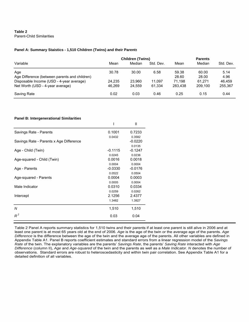
Table 2Parent-Child Similarities

Panel A: Summary Staistics - 1,510 Children (Twins) and their Parents

Variable Mean Median Std. Dev. Mean Median Std. Dev.

Age 30.78 30.00 6.58 59.38 60.00 5.14Age Difference (between parents and children) 28.60 28.00 4.96Disposable Income (USD - 4-year average) 24,235 23,960 11,097 71,198 61,271 46,459Net Worth (USD - 4-year average) 46,269 24,559 61,334 283,438 209,100 255,367

Saving Rate 0.02 0.03 0.46 0.25 0.15 0.44

Panel B: Intergenerational SimilaritiesI II

Savings Rate - Parents 0.1001 0.72330.0432 0.3582

Savings Rate - Parents x Age Difference -0.02200.0135

Age - Child (Twin) -0.1115 -0.12470.0245 0.0236

Age-squared - Child (Twin) 0.0016 0.00180.0004 0.0004

Age - Parents -0.0330 -0.01760.0522 0.0504

Age-squared - Parents 0.0004 0.00030.0005 0.0004

Male Indicator 0.0310 0.03340.0259 0.0262

Intercept 2.1256 2.43771.3482 1.3927

N 1,510 1,510

R 2 0.03 0.04

ParentsChildren (Twins)

Table 2 Panel A reports summary statistics for 1,510 twins and their parents if at least one parent is still alive in 2006 and at least one parent is at most 65 years old at the end of 2006. Age is the age of the twin or the average age of the parents. Age Difference is the difference between the age of the twin and the average age of the parents. All other variables are defined in Appendix Table A1. Panel B reports coefficient estimates and standard errors from a linear regression model of the Savings Rate of the twin. The explanatory variables are the parents’ Savings Rate, the parents’ Saving Rate interacted with Age Difference (column II), Age and Age-squared of the twin and the parents as well as a Male Indicator. N denotes the number of observations. Standard errors are robust to heteroscedasticity and within twin pair correlation. See Appendix Table A1 for a detailed definition of all variables.

Table 3Decomposition of Savings Behavior

Panel A: All Twins(N =17,630)

Model AIC LR / p-value

E 4360.00

CE -38,722 870.00

ACE -38,807

Panel B: Same Sex Twins

Model N AIC

ACE 10,786 -54,940

Panel C: By Gender

Model N AIC

Male Twins 4,710 -10,404

Female Twins 6,076 -14,110

0.0232 0.0232

Variance Components

C E

0.4185 0.0000

0.0659 0.0523 0.02360.2919 0.0242 0.6839

0.0142 0.0142

0.0157 0.0157

E

0.6448

A

0.3552

C

0.0000

0.0140

0.3642 0.0000 0.6358

A C E

Variance Components

Variance Components

0.0140

0.5815

A

1.0000

0.2200 0.7800

Table 3 reports results from maximum likelihood estimation of linear random effects models. The Savings Rate is modeled as a linear function of Male, Age, Age-squared as well as up to three random effects representing additive genetic effects (A), shared environmental effects (C), as well as an individual-specific error (E). In Panel A, we report results for a model that only allows for an individual-specific random effect (E model), a model that also allows for a shared environmental effect (CE model), and a model that also allows for an additive genetic effect (ACE model). The model is estimated using all 17,630 twins in our data set. When the non-negativity constraint for a variance parameter is binding, we report a zero. In each case, we report Akaike's information criterion (AIC), the variance fraction of the combined error term explained by each random effect (A – for the additive genetic effects, C – for shared environmental effects, E – for the individual-specific random effect) as well as the corresponding standard errors. We perform likelihood ratio tests (LR) and at the 1% level reject the E model in favor of the CE model and the CE model in favor of the ACE model. We do not report the coefficient estimates for Male, Age, and Age-squared. Panel B reports results for an ACE model estimated on only same sex twins. Panel C reports results for ACE models estimated separately for male and female twins. N provides the number of observations used in each estimation.

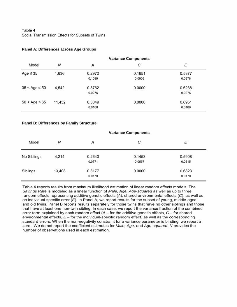
Table 4Social Transmission Effects for Subsets of Twins

Panel A: Differences across Age Groups

Model N

Age ≤ 35 1,636

35 < Age ≤ 50 4,542

50 < Age ≤ 65 11,452

Panel B: Differences by Family Structure

Model N

No Siblings 4,214

Siblings 13,408

Variance ComponentsA C E

0.2972 0.1651 0.53770.1099 0.0908 0.0378

0.3762 0.0000 0.62380.0276 0.0276

0.3049 0.0000 0.69510.0188 0.0188

C E

0.3177 0.0000 0.68230.0170 0.0170

0.0771 0.0557 0.0315

Variance Components

A

0.2640 0.1453 0.5908

Table 4 reports results from maximum likelihood estimation of linear random effects models. The Savings Rate is modeled as a linear function of Male, Age, Age-squared as well as up to three random effects representing additive genetic effects (A), shared environmental effects (C), as well as an individual-specific error (E). In Panel A, we report results for the subset of young, middle-aged, and old twins. Panel B reports results separately for those twins that have no other siblings and those that have at least one non-twin sibling. In each case, we report the variance fraction of the combined error term explained by each random effect (A – for the additive genetic effects, C – for shared environmental effects, E – for the individual-specific random effect) as well as the corresponding standard errors. When the non-negativity constraint for a variance parameter is binding, we report a zero. We do not report the coefficient estimates for Male, Age, and Age-squared. N provides the number of observations used in each estimation.

Table 5Robustness

Panel A: Controlling for Risk Aversion and Bequest

Model N

Not Controlling for Risk Aversion and Bequest 12,616

Controlling for Risk Aversion and Bequest 12,616

Panel B: Alternative Savings Measures

Model N

Savings Rate 2 17,465

Savings Rate 3 17,516

Panel C: Contact Intensity

Model N

Little contact 3,258

Intermediate contact 9,696

Frequent contact 3,298

0.0139 0.0139

0.0180 0.0180

0.0180 0.0180

0.4023 0.0000 0.5977

0.0145

0.1697 0.0000 0.8303

0.07810.2228 0.2233 0.5540

0.0145

0.6197

0.0460

Variance ComponentsA C E

0.3799 0.0000 0.6201

0.3803 0.0000

0.0405 0.02570.02180.2858 0.6924

0.0460

Variance ComponentsA

0.3516 0.0000

C E

0.0655 0.0260

C E

0.6484

Variance ComponentsA

0.0600

Table 5 reports results from maximum likelihood estimation of linear random effects models. The Savings Rate is modeled as a linear function of Male, Age, Age-squared as well as up to three random effects representing additive genetic effects (A), shared environmental effects (C), as well as an individual-specific error (E). In Panel A, we report results for the subset of 12,616 twins that hold stocks in their financial portfolios. We first report an ACE model with only Male, Age, Age-squared as explanatory variables. We then report estimates for an ACE model after also controlling for the relative fraction of the financial portfolio invested in stocks, a proxy for financial risk taking, as well as the number of children, a proxy for bequest motives. Panel B reports results for alternative proxies for savings behavior. See Appendix Table A1 for a definition of Savings Rate 2 and 3. Panel C reports results for twins that have little contact with one another (first quintile), for those that have intermediate contact (second, third, and fourth quintiles) and for those that have frequent contact (fifth quintile). In each case, we report the variance fraction of the combined error term explained by each random effect (A – for the additive genetic effects, C – for shared environmental effects, E – for the individual-specific random effect) as well as the corresponding standard errors. When the non-negativity constraint for a variance parameter is binding, we report a zero. We do not report the coefficient estimates for Male, Age, and Age-squared. N provides the number of observations used in each estimation.

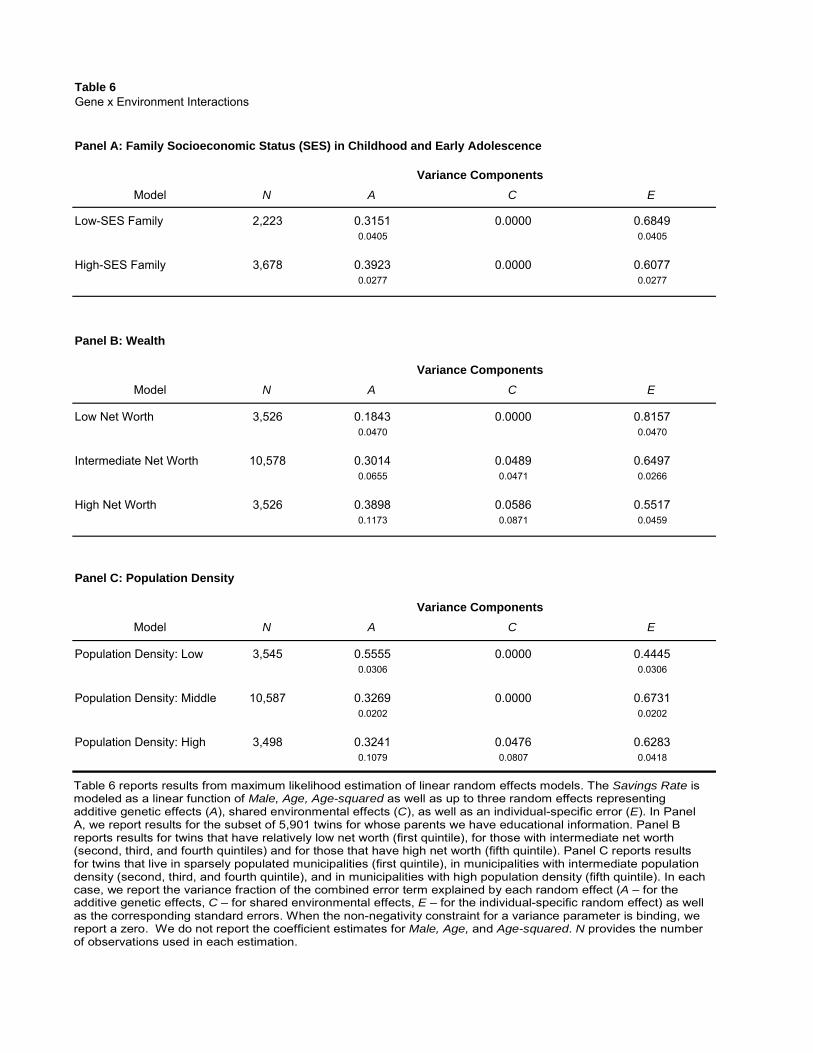
Table 6Gene x Environment Interactions

Panel A: Family Socioeconomic Status (SES) in Childhood and Early Adolescence

Model N

Low-SES Family 2,223

High-SES Family 3,678

Panel B: Wealth

Model N

Low Net Worth 3,526

Intermediate Net Worth 10,578

High Net Worth 3,526

Panel C: Population Density

Model N

Population Density: Low 3,545

Population Density: Middle 10,587

Population Density: High 3,498

0.0306

0.0202 0.0202

0.1079 0.0807 0.0418

Variance ComponentsA C E

0.1173 0.0871

0.0306

A C

0.0000

0.3241 0.0476 0.6283

Variance Components

0.0405 0.04050.3151 0.0000 0.6849

0.3923 0.0000 0.6077

A C E

0.0277

0.3014 0.0489 0.6497

0.1843 0.00000.0470 0.0470

0.55170.0459

E

0.0277

Variance Components

0.0655 0.0471 0.0266

0.3898

0.8157

0.3269 0.0000 0.6731

0.5555 0.4445

0.0586

Table 6 reports results from maximum likelihood estimation of linear random effects models. The Savings Rate is modeled as a linear function of Male, Age, Age-squared as well as up to three random effects representing additive genetic effects (A), shared environmental effects (C), as well as an individual-specific error (E). In Panel A, we report results for the subset of 5,901 twins for whose parents we have educational information. Panel B reports results for twins that have relatively low net worth (first quintile), for those with intermediate net worth (second, third, and fourth quintiles) and for those that have high net worth (fifth quintile). Panel C reports results for twins that live in sparsely populated municipalities (first quintile), in municipalities with intermediate population density (second, third, and fourth quintile), and in municipalities with high population density (fifth quintile). In each case, we report the variance fraction of the combined error term explained by each random effect (A – for the additive genetic effects, C – for shared environmental effects, E – for the individual-specific random effect) as well as the corresponding standard errors. When the non-negativity constraint for a variance parameter is binding, we report a zero. We do not report the coefficient estimates for Male, Age, and Age-squared. N provides the number of observations used in each estimation.

Table 7Net-Worth at Retirement Age

Model N

Twins: 60 - 69 years of age 12,000

Variance Components

A C E

0.3844 0.0722 0.54330.0458 0.0329 0.0188

Table 7 reports results from maximum likelihood estimation of linear random effects models. Net-Worth is modeled as a linear function of Male, Age, Age-squared as well as up to three random effects representing additive genetic effects(A), shared environmental effects (C), as well as an individual-specific error (E). We report the variance fraction of the combined error term explained by each random effect (A – for the additive genetic effects, C – for shared environmental effects, E – for the individual-specific random effect) as well as the corresponding standard errors. When the non-negativity constraint for a variance parameter is binding, we report a zero. We do not report the coefficient estimates for Male, Age, and Age-squared. N provides the number of observations.

Appendix Table A1Definition of all Variables

Variable Description

Types of TwinsIdentical Twins Twins that are genetically identical, also called monozygotic twins. Zygosity is determined by the

Swedish Twin Registry based on questions about intrapair similarities in childhood.Non-identical Twins Twins that share on average 50% of their genes, also called dizygotic or fraternal twins. Non-

identical twins can be of the same sex or of opposite sex. Zygosity is determined by the Swedish Twin Registry based on questions about intrapair similarities in childhood.

Measures of Savings BehaviorSavings Rate Savings Rate is calculated as the change in net worth between the end of 2002 and the end of

2006, less the change in home value, divided by the total disposable income for 2003 to 2006. The top and bottom 1% of the distribution have been dropped. Savings Rate is the main empirical proxy for an individual's savings behavior.

Savings Rate 2 Savings Rate 2 is calculated as the change in net worth between the end of 2002 and the end of 2006 divided by the sum of total disposable income for 2003 to 2006 and the change in home value between 2002 and 2006. The top and bottom 1% of the distribution have been dropped. Savings Rate 2 is an alternative empirical proxy for an individual's savings behavior. It is available for 17,465 out of 17,630 twins in our data set.

Savings Rate 3 Savings Rate 3 is calculated as the change in net worth between the end of 2002 and the end of 2006 divided by the total disposable income for 2003 to 2006. The top and bottom 1% of the distribution have been dropped. Savings Rate 3 is an alternative empirical proxy for an individual's savings behavior. It is available for 17,516 out of 17,630 twins in our data set.

Sociodemographic CharacteristicsMale An indicator variable that equals one if an individual is male and zero otherwise. Gender is

obtained from the Statistics Sweden.Age An individual's age on Dec. 31, 2006 as reported by the Statistics Sweden.Married An indicator variable that equals one if an individual is married in all years between 2003 and

2006 and zero otherwise. It is obtained from the Statistics Sweden.Divorced An indicator variable that equals one if an individual is divoverced in all years between 2003 and

2006 and zero otherwise. It is obtained from the Statistics Sweden.Widowed An indicator variable that equals one if an individual is widowed in all years between 2003 and

2006 and zero otherwise. It is obtained from the Statistics Sweden.High School Degree An indicator variable that equals one if an individual has at most completed high school, zero

otherwise. Educational information is obtained from Statistics Sweden.College Degree An indicator variable that equals one if an individual has at least completed high school and at

most two years of university, zero otherwise. Educational information is obtained from Statistics Sweden.

Graduate Degree An indicator variable that equals one if an individual has completed at least two years of university, zero otherwise. Educational information is obtained from Statistics Sweden.

Homeowner An indicator variable that equals one if the market value of owner occupied real estate is positive and zero otherwise. Market values are obtained from Statistics Sweden.

Disposable Income The average Disposable Income (in nominal terms) of the individual for the period 2003 to 2006, as defined by Statistics Sweden, that is the sum of income from labor, business, and investment, plus received transfers, less taxes and alimony payments. When reported in United States Dollars (USD), Swedish Krona (SEK) amounts have been converted at SEK/USD 7.1588, the average end of year exchange rate for 2003 to 2006. The data are obtained from Statistics Sweden.

Net Worth The average difference between the market value of an individual's assets and her liabilities, calculated by Statistics Sweden at the end of each year between 2003 and 2006. When reported in United States Dollars (USD), Swedish Krona (SEK) amounts have been converted at SEK/USD 7.1588, the average end of year exchange rate for 2003 to 2006. The data are obtained from Statistics Sweden.

Home Value The value of an individual's owner occupied home as reported by Statistics Sweden at the end of 2006. When reported in United States Dollars (USD), Swedish Krona (SEK) amounts have been converted at SEK/USD 6.8453, the end of year exchange rate in 2006. Home Value is missing for non homeowners. The data are obtained from Statistics Sweden.

Change in Net Worth The change in an individual's net worth between the end of 2002 and the end of 2006. When reported in United States Dollars (USD), Swedish Krona (SEK) amounts have been converted at SEK/USD 7.1588, the average end of year exchange rate for 2003 to 2006. The data are obtained from Statistics Sweden.

Change in Home Value The change in the value of the owner occupied house between the end of 2002 and the end of 2006. When reported in United States Dollars (USD), Swedish Krona (SEK) amounts have been converted at SEK/USD 7.1588, the average end of year exchange rate for 2003 to 2006. Change in Home Value is zero for non homeowners. The data are obtained from Statistics Sweden.

OtherContacts per Year The number of contacts per year between twins. The number is calculated as the average of the

numbers reported by both twins. If only one twin provides a number, this number is used. The number is available for 16,252 of the 17,630 twins in our data set.The data are obtained from the Swedish Twin Registry.

Population Density Number of individuals per square kilometer. The data are available for all twins at the municipality level (there are 289 municipalities in our data set). The data are obtained from Statistics Sweden.

Figure 1Correlations of Savings Behavior by Genetic Similarity and Gender

0.00

0.10

0.20

0.30

0.40

0.50

0.60

0.70

0.80

All Men Women

Identical Twins

Non-identical Twins - AllNon-identical Twins - Same SexNon-identical Twins - Opposite Sex