the right momentum - luiss guido carli
TRANSCRIPT
Department of Economics and Finance
Chair of Equity Markets and Alternative Investments
The Right Momentum
Candidate Emanuele Orecchini
ID 680461
Supervisor
Paolo Vitale
Co-supervisor
Marco Morelli
Accademic Year 2017-2018


i
Abstract
In this final thesis we analyze momentum investing focusing on time series application. We firstintroduce momentum risk premium, behavioral theories and then we discuss the profitability ofmomentum trading. We prove the momentum effect through Sharpe analysis, multiple regressionand backtesting procedures. We finally elaborate and present an automated momentum strategythat uses both relative and absolute momentum to generate abnormal returns.

ii
Contents
Abstract i
1 Momentum Risk Premium 31.1 Introduction . . . . . . . . . . . . . . . . . . . . . . . . . . . . . . . . . . . . . . . . . 31.2 Relative and Absolute Momentum . . . . . . . . . . . . . . . . . . . . . . . . . . . . 41.3 The Effect of Correlation . . . . . . . . . . . . . . . . . . . . . . . . . . . . . . . . . . 41.4 Behavioral Theories and Market Efficiency . . . . . . . . . . . . . . . . . . . . . . . 6
2 The Momentum Effect 102.1 Introduction . . . . . . . . . . . . . . . . . . . . . . . . . . . . . . . . . . . . . . . . . 102.2 Momentum Trading . . . . . . . . . . . . . . . . . . . . . . . . . . . . . . . . . . . . 102.3 Empirical Evidence . . . . . . . . . . . . . . . . . . . . . . . . . . . . . . . . . . . . . 122.4 Published Studies . . . . . . . . . . . . . . . . . . . . . . . . . . . . . . . . . . . . . . 13
2.4.1 Time Series Momentum . . . . . . . . . . . . . . . . . . . . . . . . . . . . . . 13Volatility Model . . . . . . . . . . . . . . . . . . . . . . . . . . . . . . . . . . . 13Regression Analysis . . . . . . . . . . . . . . . . . . . . . . . . . . . . . . . . . 14Momentum Strategy . . . . . . . . . . . . . . . . . . . . . . . . . . . . . . . . . 15
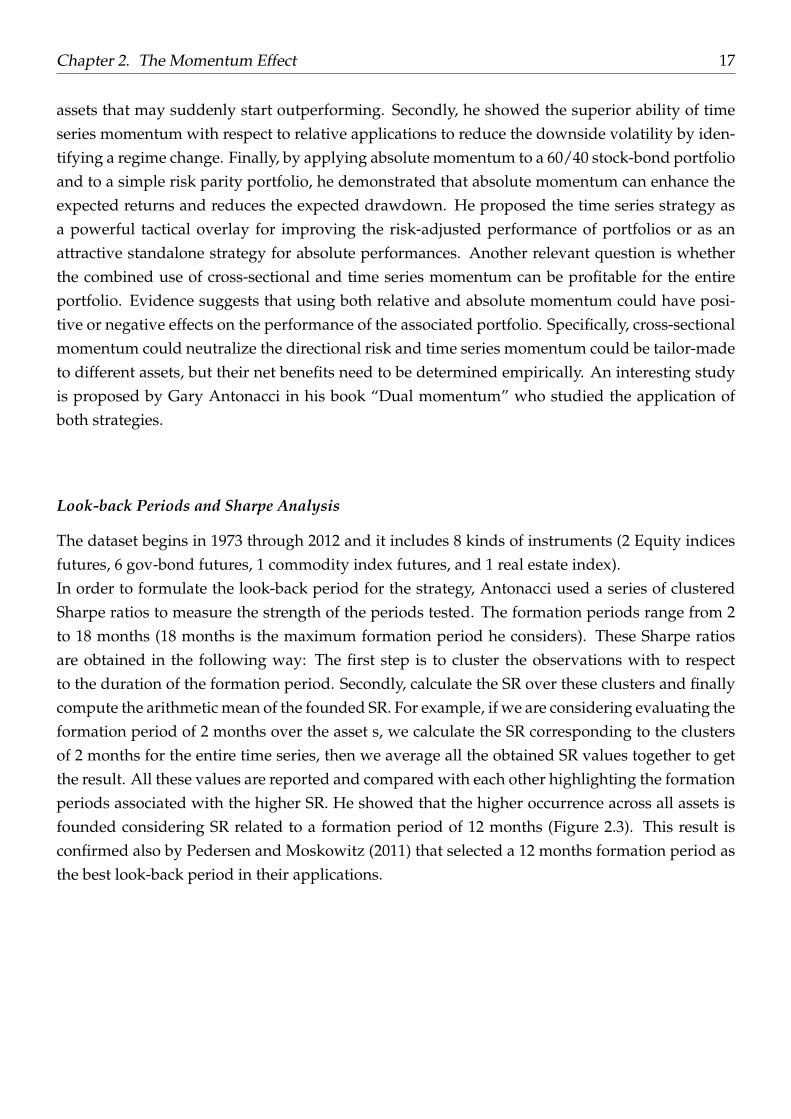
2.4.2 The Dual Approach . . . . . . . . . . . . . . . . . . . . . . . . . . . . . . . . 16Look-back Periods and Sharpe Analysis . . . . . . . . . . . . . . . . . . . . . . . 17Absolute Momentum on a 60/40 Portfolio . . . . . . . . . . . . . . . . . . . . . . 18Dual Momentum . . . . . . . . . . . . . . . . . . . . . . . . . . . . . . . . . . . 18
2.5 The Momentum Effect: A practical application . . . . . . . . . . . . . . . . . . . . . 262.5.1 Data and Methodology . . . . . . . . . . . . . . . . . . . . . . . . . . . . . . 262.5.2 Sharpe Evaluation on Formation Periods . . . . . . . . . . . . . . . . . . . . 262.5.3 Volatility Model . . . . . . . . . . . . . . . . . . . . . . . . . . . . . . . . . . . 302.5.4 Regression Analysis . . . . . . . . . . . . . . . . . . . . . . . . . . . . . . . . 33
3 Momentum Strategy 353.1 Data and Methodology . . . . . . . . . . . . . . . . . . . . . . . . . . . . . . . . . . . 353.2 Backtesting . . . . . . . . . . . . . . . . . . . . . . . . . . . . . . . . . . . . . . . . . . 353.3 Best Index Best Strategy Algorithm . . . . . . . . . . . . . . . . . . . . . . . . . . . . 38
3.3.1 Test for t = 1 . . . . . . . . . . . . . . . . . . . . . . . . . . . . . . . . . . . . . 403.3.2 Modified Relative Momentum . . . . . . . . . . . . . . . . . . . . . . . . . . 42

iii
3.4 Results and Implementations . . . . . . . . . . . . . . . . . . . . . . . . . . . . . . . 42
Bibliography 53

1
Introduction
Whether we decide to invest our savings or our time into a project, a new business opportunityor into something that seems to be appealing to us, we strongly believe that our choice will bepromising. When we do that we are betting, and every bet implies some risk. What we gather atthe end it’s the willingness to accept the risk, a premium.In Finance the risk premium it is defined as “the return in excess of the risk-free rate of return thatan investment is expected to yield” 1. Maximizing this premium for a given level of risk it is alwaysbeen the principal objective of modern portfolio theory. It’s also well-known that Economics it’snot an exact science, but a social science and the word social means human, which in turn impliesirrationality, which again is the expression of our behavior. In recent years we filled this gap andwe start to move away from the traditional view of risk premium into a new one, the so-calledalternative risk premium.Traditional risk premia are returns that can be harvested passively from directional long expo-sures in asset classes such as stocks, bonds, commodities and so forth. By contrast, ARP 2 is adynamic and systematic source of return that behaves differently from those in traditional mar-kets 3 . While traditional risk premium includes factor investing 4 or smart beta strategies 5 thatare related to systematic risk, the latter is structured as a long-short investment and it may beindependent of traditional risk premia. Moreover, ARP should not be confused with alpha strate-gies, which are believed to be driven by a manager’s security selection and market-timing skills.The ARP on traditional financial assets such as commodities, equity or currencies often resultsfrom market behaviors and structured conditions of the market itself. If we start selling losers
1Risk Premium, Investopedia [Internet]. Available from:https://www.investopedia.com/terms/d/drawdown.asp[Accessed 20 September 2018]. Alternative Risk Premia.
2Alternative Risk Premia.3Communication department (2017), Alternative Risk Premia: What Do We Know? Viewpoint Amundi Asset
Management [Internet]. Available from: http://research-center.amundi.com/ [Accessed 20 September 2018].4Factor investing is an investment approach that involves targeting quantifiable firm characteristics
or “factors” that can explain differences in stock returns. Over the last 50 years, academic researchhas identified hundreds of factors that impact stock returns, Wikipedia [Internet]. Available from:https://en.wikipedia.org/wiki/Factor_investing [Accessed 20 September 2018].
5Smart beta investing combines the benefits of passive investing and the advantages of active investing strate-gies Investopedia [Internet]. Available from: https://www.investopedia.com/terms/d/smartbeta.asp [Accessed 20September 2018].

Contents 2
and buying winners, we are creating momentum. If we are betting on a cheap asset that has po-tential growth and a higher fair price, we are considering value investing. If we think that anasset yield is mispriced, we believe in carry opportunities.These are the most common sources of ARP and are also well-known for many years among in-vestors, the key difference is how they are implemented. In fact, if ARP strategies are includedin portfolios alongside traditional investments, they enhance diversification and provide benefits(e.g. reduce drawdown exposure 6 ) since they exhibit heterogeneous statistical properties.After the 2008 global financial crisis, the diversification has become the primary objective of insti-tutional investors and wealth funds who needed to restructure their portfolio in a low correlatedenvironment. To complicate the situation, it was also the uncertainty of future behavior of thestock-bond correlation that continues to be negative since the 90’s and should revert to positiveover the long run 7 . As a reaction wealth funds and sophisticated investors have switched fromcommon diversification procedures to a deleveraging equity solution using sovereign bond ashedging assets and corporate bond as lower beta assets (sovereign bonds are felt more as assetsfor hedging than for performance).ARP are expanding the universe of traditional risk premia and are becoming the building blocksof multi-asset management. In 2017, a survey from bFinance 8 suggests that ARP has been the areaof the greatest interest among investors on a rolling 12-month basis. In the same year, DeutscheBank reported some survey results 9 showing the growth of the percentage of investors who al-locate to ARP strategies, with an increase of 20% from 2015 the level has reached the 26 % in2017. Furthermore, a recent Prime Brokerage survey 10 from Morgan Stanley reports that 79%of investors with more than $5 billion of assets under management in hedge fund investmentscurrently rely on ARP strategies or are considering to allocating on ARP.
6Drawdown, Investopedia [Internet]. Available from: https://www.investopedia.com/terms/d/drawdown.asp[Accessed 20 September 2018].
7If economic conditions and monetary policy permit this change.8“Manager Intelligence and Market Trends”, bFinance (February 2017).915th Annual Alternative Investment Survey,” Deutsche Bank (March 2017).
10“Recent Hedge Fund Trends,” Morgan Stanley Prime Brokerage-Strategic Content Group (July 2017).

3
Chapter 1
Momentum Risk Premium
1.1 Introduction
“A popular view is that individuals tend to overreact to information” and “if stock prices either overreactor underreact to information, profitable trading strategies that select stocks based on their past returns willexist.” Titman and Jegadeesh 1993.1
In 1993 Titman and Jegadeesh first introduced the concept of Relative Momentum focusing onpositive returns of stocks generated by buying recent winners and selling recent losers. Nowa-days Momentum is considered among investors one of the oldest and most popular trading strate-gies over the entire industry. Often in contrast with contrarian investors that consider overreac-tion and underreaction of assets as something temporary, that will mean revert in the future.Contrarian’s strategy is based on the fact that some stocks are mispriced by the market and willrevert to their fair value in the future. Specifically, by buying recent losers and selling recentwinners they try to anticipate this process of mean-reversion. Decisions are made estimating thefundamental value of an asset and comparing it to his market value. Therefore, the contrarian ap-proach is considered a form of value investing. Differently, momentum investors follow the trendand the market by betting on the under-reaction or on the over-reaction itself. This explains whythey are considered as “lazy” investors and their strategies as trend following approaches. It mayappear that “value and contrarian investing are gratifying while momentum investing is shameful” 2 butif we look at the composition of the quarterly portfolio holdings of 155 equity mutual from 1974 to1984 we discover that the 77% of them were momentum investors (Grinblatt and Wermers, 1995).
1Jegadeesh and Titman, 19932Philippe Ithurbide et al. (2017), Keep Up The Momentum, Discussion Paper - cross asset Investment Strategy.

Chapter 1. Momentum Risk Premium 4
1.2 Relative and Absolute Momentum
In order to fill the gap between momentum strategies and momentum risk premia, we need to dis-tinguish momentum time series from cross-sectional momentum. These strategies both assumethat the past trend is a predictor of the future trend and that the initial underreaction (anchoring3)and subsequent overreaction (herding4) may lead to price move continuation. What differs interms of risk premia is the net exposure.In time series momentum the net exposure is not equal to zero whereas in cross-sectional momen-tum it is equal to zero. In fact, time series momentum strategies are implemented considering onlysingle assets and using their past history as a benchmark, e.g. buying an asset with recent positiveperformance or sell it if the recent performance is negative. These strategies create a positive ornegative net exposure depending on the direction of the trend that has been followed.Differently, cross-sectional momentum is not implemented on a standalone basis, but by consid-ering a set of assets and by assuming that current winners will continue to outperform currentlosers, e.g. buying assets that have the best recent returns and selling the same number of assetsthat exhibit the worst performances. These strategies create portfolios that go long on outper-formers and go short on underperformers ensuing a zero-net exposure. We may state in a verysimple manner that absolute momentum allows comparing performance with himself, while rel-ative momentum allows comparing performance with his peers.
1.3 The Effect of Correlation
Another distinction among momentum applications is made in terms of correlation. In particular,Roncalli et al. starting from the model of Brouder and Gaussel5 showed how the impact of cor-relation varies between relative and absolute momentum. Their results are derived analyticallyfrom the assumption that an asset price st follows a geometric Brownian motion with constantvolatility and with a time-varying trend.Absolute momentum does not benefit from correlation6: if we look at Figure 1.1 we notice thatthe diversification gain is limited when adding more than three assets confirming the fact that thiskind of strategy is indifferent from a positive or a negative correlation. Furthermore, Jusselin etal (2017) starting from the analytical model of Brouder and Gaussel went deeper inside the ques-tion of how the correlation of asset affects absolute momentum. The main result is that the signof correlation does not influence the performance of a trend following strategy, specifically theydemonstrated that the profit & loss scheme of such strategy does not depend on the sign of the
3It refers to a behavioral finance phenomenon called anchoring behavior.4It refers to a behavioral finance phenomenon called herding behavior.5Bruder and Gaussel, 20116The tests on correlation are derived analitically.

Chapter 1. Momentum Risk Premium 5
correlation: a correlation of 80% has the same impact of a correlation of -80% (Figure 1.2 showsthis effect).Differently, relative momentum is a “friend of correlation” since his Sharpe ratio increases simul-taneously with the correlation (Figure 1.3). The performance of a cross-sectional strategy dependsmore on the relative differences between the trends of the selected assets, i.e. the spread betweenonly positive or negative trends as well as the spread between the trends of the winners and thetrends of the losers7 . Moreover, a high correlation among assets 8 will reduce the uncertaintyof the outcome and the subsequent dispersion of the profit & loss of the strategy capturing thespread-risk between trends9 and leaving the directional risk10 of trend aside. In this last caseits useful to compare the relative strategy with pairs trading (considering each pair as one invest-ment bet). This trading approach looks similar to the one used in cross-sectional momentum sincethe performance of the strategy is related to a long/short matching of assets.Since absolute momentum follows the market or the trend direction creating positive or nega-tive net exposure, in case of big trends the time-series strategy should concentrate its exposureentirely on the asset that exhibits the trend (single bet) rather than diversifies the exposure on dif-ferent assets (multiple bets). This is not the case of relative momentum that should be exposed tomany relative bets in order to capture their spread risk. The choice of the universe is then impor-tant when considering a trend-following strategy. In a portfolio construction process, time seriesmomentum should be used over a multi-asset universe (i.e. equity, currency, and commodity),whereas cross-sectional momentum strategies should be applied in a universe of homogeneoussecurities (i.e. geographical or sectorial divisions). A possible approach would follow an imple-mentation of absolute momentum at a global level and relative momentum at a categorical level.From now on we will focus only on absolute momentum and on his applications (Roncalli et al.2017).
7The fact that relative momentum captures two opposite trends at the same time is quite difficult in reality (Ron-calli, 2017a).
8With high correlation we mean that all the assets within the dataset need to be positively or negatively correlatedin order to better capture the spread risk between trends. Best results are found when the correlation is positive andhigh (Roncalli, 2017b).
9Relative difference between trends.10It is the risk of taking the “wrong” direction of the market.

Chapter 1. Momentum Risk Premium 6
1.4 Behavioral Theories and Market Efficiency
Momentum is based on the autocorrelation between asset returns which in turns assumes thatthere will be a trend continuation in the future (positive or negative). This concept goes againstthe two biggest assumptions of modern finance: the efficient market hypothesis and the randomwalk hypothesis. The efficient market hypothesis states that markets are efficient and that all pri-vate and public information is incorporated in the asset price. This excludes the possibility amonginvestors to obtain abnormal rates of returns from the market11. EMH12was often equated toRWH13 since they share common principles.The random walk hypothesis implies that aggressivecompetition among market participants to exploit any predictable patterns makes price changesfully random and unpredictable14. However, the EMH allows time variation in rational risk pre-mia whereas the RWH assumes the case of constant expected returns. Thus, according to theevidence of return predictability only RMH is rejected (Anti Ilmanen 2011). Since financial mar-kets are not exact and predictable we may encounter in some errors which are often described asanomalies or inefficiencies of the market.Anomalies are distortions associated with the impossibility of an asset price to reflect his fairvalue. These errors suggested a more dynamic view of the market, formalized in the Adaptivemarket hypothesis. AMH15applies evolutionary and ecological principles to financial marketsshowing that human behavioral interactions “stimulate” the market and may reduce his degreeof efficiency. Following EMH, anomalies are the reason for their own elimination and the ensuingfinite process of exploitation self-stabilizes the market.However, boom events such as the Tech bubble and the 2008 Global financial crisis caused a “lackof fundamentalism” among market operators carrying on the idea of persistence of these ineffi-ciencies. An interesting point of view is expressed by Atti Ilmanen in his book (Expected Returns2011):
“To me, a fair conclusion is that recent events have undermined the validity of the EMH’s main idea(that market prices are always “right”, near the fair value), but have underlined the validity of its mainimplication for most investors (that beating the markets is extremely difficult, no free lunches). It is ironicthat while the EMH is seen as one scapegoat for the 2008 crisis, behavioral finance has survived unscathed,with its reputation even enhanced. Although the EMH paradigm has faced a vigorous challenge from be-havioral finance, there is no doubt that the EMH has been a powerful organizing principle for theoreticaland empirical work in finance that has improved our understanding of asset returns.”
Obviously, Behavioral finance shakes things up and turned the inefficiencies of the market into
11Strong form of Efficient market hypothesis.12Efficient market hypothesis.13Random walk hypthesis.14Ilmanen, A. (2011), Expected returns: An investor’s guide to harvesting market rewards. John Wiley & Sons.15Adaptive market hypothesis.
Chapter 1. Momentum Risk Premium 7
social and psychological behaviors. Anomalies such as Momentum are explained by BF16 as aninitial underreaction (anchoring) and a subsequent over-reaction (herding) of the value of an as-set that may cause price move continuation. These anchoring and herding behaviors are fueledby the market itself. In particular, herd behavior is the tendency for individuals to mimic theactions (rational or irrational) of a larger group. In the financial market, this occurs when marketoperators “follow the trend” and copy the behavior of other investors by buying and selling thesame asset. Similarly, anchoring demonstrates the tendency to attach or "anchor" our thoughts toa reference point, even if it may have no logical relevance. It is a cognitive bias where individualsplace too much weight on the first piece of information that they get to make investment deci-sions17. In financial markets, the investor puts more weight on the latest or the most outstandingstock price, which becomes the anchor in making future stock predictions and leads to an initialunder-reaction. Furthermore, the disposition effect that relates to the tendency of investors to sellshares whose price has increased while keeping assets that have dropped in value, may fuel themomentum anomaly by exacerbating the under-reaction since investors are more reluctant to selland are more likely to realize large losses.Other cognitive biases such as representativeness and misperception of regression to the meancontribute to generating momentum. The former is where an investor assumes the probabil-ity of the stock going in a certain direction by judging it relative to its performance in the past,whereas the latter describes how individuals do not acknowledge fully the degree to which thereis a regression to the mean. Despite there is no general consensus, behavioral biases may be theprincipal cause of the momentum effect18
16Behavioral Finance.17Hazel Kadzikano (2017), Behavioral theories behind momentum. Quantsportal [Internet]. Available from:
http://www.quantsportal.com/behavioural-theories-behind-momentum/ [Accessed 20 September 2018].18Breaking Down Fiance [Internet]. Available from:http://breakingdownfinance.com/finance-topics/behavioral-
finance/anchoring/ [Accessed 20 September 2018].

Chapter 1. Momentum Risk Premium 8
The effect of correlation on absolute applications
FIGURE 1.1: displays the Cumulative Distribution Function of a trend following strat-egy showing limited diversification gain when adding more than three assets. Theseresults are derived analytically from the model of Brouder and Gaussel by Roncalli et
al. 2017.
The correlation symmetry on absolute momentum
FIGURE 1.2: displays the cumulative distribution function of a trend following ap-plication zero showing that this kind of strategy is indifferent from a positive or anegative correlation. These results are derived analytically from the model of Brouder
and Gaussel by Jusselin et al. 2017.

Chapter 1. Momentum Risk Premium 9
The effect of correlation on relative applications
FIGURE 1.3: shows that relative momentum is a “friend of correlation” since theSharpe ratio increases simultaneously with the correlation. These are the highest re-sults and have been obtained when the correlation across assets was high and posi-tive. Cross-sectional momentum worked well in capturing the spread-risk of the asset
trends (Roncalli et al 2017).

10
Chapter 2
The Momentum Effect
1
2.1 Introduction
Momentum trading strategies have always been historically successful in almost every assetclasses demonstrating an excellent power of diversification and heterogeneous statistical prop-erties.Statistical evidence suggests that many financial assets show positive short-term autocorrelation(momentum bias) and negative long-term autocorrelation (mean reversion bias). Momentumbias2 is generally confirmed except for very short (less than a week) and very long (greater thantwo years) windows where reversal biases3 dominate. Most of these studies use monthly datawithout adjusting momentum signals and position sizes for volatility.
2.2 Momentum Trading
Academic studies often use past average returns as trading signals, but we know that there arevarious methodologies to create signals that do not outperform each other. In particular, the mostcommon trend following rule is based on moving average (where the current market price of thestock it is compared with the average of his historical prices): if the current price is above (below)the moving average, we have a buy (sell) signal. Some momentum rules use a different kind of
1We refer to absolute momentum effect.2Using the expression of momentum biases, we refer to the momentum effect that can be interpreted as an
anomaly or as a bias of the market.3When the market suddenly revers: it changes trend direction (from positive to negative or vice-versa)Potters and
Bouchaud, 2006.

Chapter 2. The Momentum Effect 11
lagging indicators such as a shorter moving average or an exponential moving average in orderto improve the entire fit of the model4. In contrast, the use of technical momentum indicators thatmeasures the magnitude of recent price changes to analyze overbought or oversold conditionssuch as the relative strength indicators5, underweights the magnitude of market moves empha-sizing the frequency of up moves and down moves. Hence, this kind of measures is less effectiveto create momentum signals.Another entry rule concerns acceleration or breakout signals filtering the recent price moves andthe preceding market action. When a stock price “breaks” the so-called psychological level orresistance it could indicate a possible start of a trend and when this phenomenon is carried withsharp market moves it often represents a momentum signal. In addition to entry rules, exit rules(stop losses or take profit) are fundamental in order to minimize the loss when reversals occur.Trend followers typically diversify not just across a large number of assets but also across differenthistorical window length and trading frequencies. The use of look-back periods varies depend-ing on the underlying asset and the applied strategy. They could range from months to intradaytrading in case of high-frequency data. The main rule is that optimizations and trend followingmodels need to be dynamic and constantly rebalanced considering the state of the market at everytime, usually, this kind of models are implemented and reviewed at least once a month.One of the most important decisions regarding trend following applications is the volatility weight-ing procedure for positions and return signals. Since volatility varies across assets and over time(especially using slightly different asset classes like commodities and currencies) targeting theposition and the return signal with to respect to the volatility of the underlying asset could be asource of benefits for the entire strategy.There is some evidence6 that volatility targeting reduces risk and enhances the results of com-modities strategies.Firstly, if return signals are not adjusted to volatility, a less volatile asset will be preferred to ahigher one. Specifically, the use of momentum strategies over a set of assets could penalize theinstruments that present higher volatility excluding them from the active portfolio.An example could be made considering again natural gas and gold. The former (which is highlyvolatile) will be more likely to be at either end of the rankings than the latter (which is three tofour times less volatile). This bias of exclusion reduces the breadth of the entire asset universe.Secondly, if position sizes are not adjusted for differences in volatility across assets there is likelyto be a long directional bias: the long or short positions produced by the ranking model can bemarket directional. Every long/short matching that does not include volatility weighting proce-dures will suffer from directional bias. This is true especially if we are considering heterogeneous
4The use of different kind of moving averages highly depends on the type of stock that is under scrutiny.5Are calculated considering the average gain of up periods during the specified time frame / av-
erage loss of down periods during the specified time frame, Investopedia [Internet]. Available from:https://www.investopedia.com/terms/d/RSI.asp [Accessed 20 September 2018].
6Ilmanen’s study on commodities, Ilmanen, A. (2011), Expected returns: An investor’s guide to harvesting marketrewards. John Wiley & Sons.

Chapter 2. The Momentum Effect 12
universes such as commodities. In these asset classes, the directional bias will be stronger ratherthan bonds since in general commodities present greatest volatility differences among each other.(e.g. a dollar neutral long natural gas versus a short gold position is not empirically neutral togenerally changing commodity prices; it effectively has a long directional bias).Volatility weighting of positions also helps to reduce the nominal position sizes when recentvolatility is higher creating volatility stabilization and enhancing risk-adjusted returns. A dy-namic form of volatility weighting is to stop a trend following strategy after high recent volatilityor better to create relative weights (fast and slow signals) as a function of the volatility level in thehistorical window to favor slow signals during bull markets and fast signals during bear markets(Ilmanen 20117).
2.3 Empirical Evidence
There is evidence8 that comes from the spurious use of momentum trading in different assetclasses that suggest some recommendations during the applications of these strategies.First of all, the attention needs to be focused on liquid assets since it is true that less liquid assetsare more likely to trend, but their exploitation may be a difficult process to grasp (also consideringthe high level of transaction costs), that’s why most of the strategies use highly liquid asset likefutures and currencies. Secondly, theoretically poorly anchored asset prices allow grater trendingbecause they give more scope for sentiment-driven changes, the lack of fair value of an asset maylead it to trend sharply. The explanation of this phenomenon is based on Behavioral finance biasessuch as the disposition effect and the anchoring behavior that may cause abnormal sentiment.In particular, the investor’s reluctance to realize small losses (disposition effect) exacerbates mo-mentum effects. It fuels the underreaction or the moment which correspond to the differencebetween the current price and the price at which most investors bought.Other conditions of the market may be helpful and can enhance the performance of absolutemomentum applications. For example, it is well known that momentum works better betweentrends rather than range-bound markets, then macro trends and conditions should be constantlymonitored. Another element to take under consideration is seasonality, it has been demonstratedthat trend following strategies tend to perform better in December rather than January. The mainexplication is given by year-end tax-loss selling9 and by the phenomenon of window dressingwhere institutions buy (sell) assets that have outperformed (underperformed) in order to make
7Ilmanen, 20118Ilmanen, A. (2011), Expected returns: An investor’s guide to harvesting market rewards. John Wiley & Sons.9Tax selling refers to a type of sale in which an investor sells an asset with a capital loss in order to lower or
eliminate the capital gain realized by other investments, for income tax purposes. Tax selling allows the investorto avoid paying capital gains tax on recently sold or appreciated assets, Investopedia [Internet]. Available from:https://www.investopedia.com/terms/d/drawdown.asp [Accessed 20 September 2018].

Chapter 2. The Momentum Effect 13
their portfolio better looking at the eyes of investors. Furthermore, momentum strategies tendto perform better when volatility starts to rise after a period of contained volatility. Finally, mo-mentum time series tend to perform well when big events or announcements affect the assets,abnormal SR are documented for gov-bond and for commodities at the beginning of the eventwindow (Ilmanen 2011).
2.4 Published Studies
Momentum strategies perform well in almost all asset classes. Moskowitz and Pedersen et al,as well as Gary Antonacci, studied the trend following applications on equities, currencies, com-modities, and bonds finding substantial abnormal returns, especially during extreme markets.The empirical evidence suggests that trend following strategies using equity index futures areprofitable in many countries, it also works in commodities, fixed income, foreign exchange, andalternative assets, as well as across asset classes.
2.4.1 Time Series Momentum
Pedersen and Moskowitz et al10. (2011) focused on absolute momentum strategies confirming thevalidity and effectiveness of the application regarding every asset classes. They further demon-strated the momentum effect and the subsequent reversals for each asset within the database.Their data begins in 1965 through 2009 and includes 58 instruments (24 commodities futures, 12cross-currencies pairs forwards, 9 equity indices futures, and 13 gov-bond futures). In particular,they showed that in absolute momentum there is significant positive auto-covariance between anasset’s return in the following month and his past one-year excess return. Following this state-ment, looking at an asset’s excess return over the entire look-back period is the main task forapplying absolute rules11.
Volatility Model
In order to analyze momentum strategies, volatility needs to be taken under scrutiny since itlargely varies across contracts and among asset classes. It is well known that some asset classessuch as commodities and equities present higher volatility than bond futures or currency for-wards, but what is often slipping away among investors is that even among the same asset class
10Moskowitz and Pedersen, 201211When this excess return is positive, we have a positive absolute momentum effect.

Chapter 2. The Momentum Effect 14
(e.g. commodities) there is substantial cross-sectional variation in terms of volatility. For example,the volatility of natural gas futures is about 50 times larger than 2-year US bond futures.To make meaningful comparison across instruments with different volatilities and combine vari-ous assets into a diversified portfolio, Moskowitz et al. elaborated a volatility model and a filter-ing procedure.In particular, they scaled the returns by their volatilities estimating each instrument’s ex-ante orconditional variance σ2
t at each point in time using a model called the exponentially-weightedlagged squared daily returns.Specifically, they calculated the conditional annualized variance for each instrument as follows:
σ2t = 261
∞
∑i=0
(1− δ)δi(rt−1−i − r̄t)2 (2.1)
where the scalar 261 scales the variance to be annual, the weights (1− δ)δi add up to 1, r̄t is theexponentially weighted average return computed similarly and rt−1−i is the return at time t-1-i.The parameter δ is chosen so that the center of mass of the weights is:
∞
∑i=0
(1− δ)δi =δ
1− δ= 60 (2.2)
To ensure that no look-ahead bias contaminates the results, they used the volatility estimates attime t-1 applied to time t returns throughout the analysis. This model is applied to all the assetswithin the database.
Regression Analysis
In order to show that in absolute momentum there is significant positive auto-covariance betweenan asset’s return in the following month and his past one-year excess return, they applied regres-sion analysis. They found that the past 12-month excess return of each instrument is a positivepredictor of its future return. This time series momentum effect persists for about a year and thenpartially reverses over the long horizons.After having estimated the conditional volatility for each asset, they divided all the returns fortheir estimated volatility. To show the time series predictability of asset returns, they run a pooled

Chapter 2. The Momentum Effect 15
panel regression (similarly to a Generalized Least Square) and compute t-statistics that accountfor group-wise clustering by time (at the monthly level). They used two different procedures. Thefirst regression is run using lags of h, where h goes from 1 to 60 months and it is described by thefollowing formula:
rst
σst−1
= α + βrs
t−hσs
t−h−1+ εs
t (2.3)
Where the dependent variable rst is the excess-return of the asset s on the month t scaled by the
estimated volatility, regressors are lagged excess returns of the asset s at time t-h. The secondprocedure looks similar, but it focuses on the sign of the past excess return. In this framework,they again made the regression independent to volatility, so that all the estimates are comparableacross instruments and among different asset classes. The regression is run using lags of h, whereh goes from 1 to 60 months and it is described by the formula:
rst
σst−1
= α + βhsing(rst−h) + εs
t (2.4)
The results of the two regression procedures are similar and both show strong evidence of returncontinuation for the first year and reversals for the next four years. In both cases, the data exhibita clear pattern, with most recent 12-month lag returns positive (and nine statistically significant)and most of the remaining lags negative. These findings slightly vary between asset classes andare robust across different lock-back periods and holding periods. Moreover, these results arepositive not just on average, but for each asset class they have examined.The findings of positive trends that partially reverse over the long-term may be consistent withinitial under-reaction and delayed over-reaction, which behavioral theories suggest and that canproduce these return patterns (anchoring, herding behavior, and the disposition effect). The re-sults of the two pooled panel regressions are described in Figure 2.1.
Momentum Strategy
After showing the time series predictability they focused on the profitability of some tradingstrategies based on absolute momentum. In order to test the strategy, they varied both the “look-back period” and the “holding period” on every instrument within the dataset. Moreover, for

Chapter 2. The Momentum Effect 16
each asset s and month t, they considered the excess return over the past k months and depend-ing on the sign of this excess return they hold the position for h months. Specifically, the twofundamental periods are described as follow:
• Look-Back Period: it is the time considered for creating a signal. It is constructed creatingaverage functions of returns for each asset during k months. The signals are generatedwhether the excess return of these averages is positive or negative, in case of positive signalwe go long, while in case of negative signal we go short.
• Holding Period: it represents how long the position remains open and it varies from theparameter h.
They sized each position with to respect to estimated volatility to create an easier aggregationbetween strategies and across instruments with very different levels of volatility. This choice ishelpful econometrically since having a time series with stable volatility ensure that the strategyit is not dominated by a few volatile periods and reduces the risk of being market directional12.For each trading strategy (k, h) they derived a single time series of monthly returns even if theholding period h is more than one month. Moreover regarding equity returns, some researchpapers13 and studies often choose to skip the most recent month of the selected look-back periodin order to create a separation between the momentum effect and the subsequent reversal. Thismethod is useful in cases of liquidity issues since there may be more complex to close and openpositions. In this analysis Moskowitz et al. choose to rebalance positions without skipping thelast month of observation (this choice highly depends on the type of asset considered during thetest).In particular, they focus on the properties of the 12-month time series momentum strategy witha 1-month holding period (i.e. k = 12 and h = 1) for all the assets within the database. Figure 2.2plots the cumulative excess return of the strategy for all futures contracts they have examined (ona log scale) scaled by the same conditional volatility. In order to have comparable metrics, theyplotted also the cumulative excess returns of a diversified passive long position in all instrumentswith equal risk on every asset, the instruments are scaled by the same conditional volatility.
2.4.2 The Dual Approach
Gary Antonacci (2014) questioned the diversifier power of relative momentum enhancing theproperties of absolute applications. He first discussed how the procedure of choosing winnersand losers may create a segmentation of the set of assets reducing the benefits that come from amulti-asset diversification. This phenomenon may lead to opportunity loss by excluding lagging
12Market directional bias.13Antonacci, 2013.
Chapter 2. The Momentum Effect 17
assets that may suddenly start outperforming. Secondly, he showed the superior ability of timeseries momentum with respect to relative applications to reduce the downside volatility by iden-tifying a regime change. Finally, by applying absolute momentum to a 60/40 stock-bond portfolioand to a simple risk parity portfolio, he demonstrated that absolute momentum can enhance theexpected returns and reduces the expected drawdown. He proposed the time series strategy asa powerful tactical overlay for improving the risk-adjusted performance of portfolios or as anattractive standalone strategy for absolute performances. Another relevant question is whetherthe combined use of cross-sectional and time series momentum can be profitable for the entireportfolio. Evidence suggests that using both relative and absolute momentum could have posi-tive or negative effects on the performance of the associated portfolio. Specifically, cross-sectionalmomentum could neutralize the directional risk and time series momentum could be tailor-madeto different assets, but their net benefits need to be determined empirically. An interesting studyis proposed by Gary Antonacci in his book “Dual momentum” who studied the application ofboth strategies.
Look-back Periods and Sharpe Analysis
The dataset begins in 1973 through 2012 and it includes 8 kinds of instruments (2 Equity indicesfutures, 6 gov-bond futures, 1 commodity index futures, and 1 real estate index).In order to formulate the look-back period for the strategy, Antonacci used a series of clusteredSharpe ratios to measure the strength of the periods tested. The formation periods range from 2to 18 months (18 months is the maximum formation period he considers). These Sharpe ratiosare obtained in the following way: The first step is to cluster the observations with to respectto the duration of the formation period. Secondly, calculate the SR over these clusters and finallycompute the arithmetic mean of the founded SR. For example, if we are considering evaluating theformation period of 2 months over the asset s, we calculate the SR corresponding to the clustersof 2 months for the entire time series, then we average all the obtained SR values together to getthe result. All these values are reported and compared with each other highlighting the formationperiods associated with the higher SR. He showed that the higher occurrence across all assets isfounded considering SR related to a formation period of 12 months (Figure 2.3). This result isconfirmed also by Pedersen and Moskowitz (2011) that selected a 12 months formation period asthe best look-back period in their applications.

Chapter 2. The Momentum Effect 18
Absolute Momentum on a 60/40 Portfolio
Once the optimal look-back period is founded he applied the 12 months absolute momentum toimprove the performance of a 60/40 portfolio. In this application, he focused only on long mo-mentum strategies without considering short exposures. This portfolio is composed of 60% of theUS MSCI and of 40% of the US Treasury indexes. To show the differences he compared the 60/40portfolio with and without absolute momentum. With to respect to investments in US stocks, the60/40 portfolio without momentum proves some reduction in volatility and drawdown risk. Inany case, the solid 0.92 correlation founded of the 60/40 portfolio with the S&P 500 demonstratesthat the 60/40 portfolio is bearing the market risk of US stocks. Moreover since stocks are morevolatile, they dominate the risk in this kind of portfolios that behaves almost as an equity port-folio. When 12 months absolute momentum is added, the MSCI US showed a 0.67 correlation tothe S&P 500 (lower than 0.92) and presented superior ability to reduce drawdown by more than70% enhancing the returns of the overall strategy. Figure 2.4 and Figure 2.5 presents the results interms of drawdown and abnormal returns. Figure 2.4 by Antonacci and Figure 2.2 by Moskowitzfollow different methodology and instruments, but they share common features. In particular, ifwe look at these figures analyzing the impact of the most recent global financial crisis, we see thattime series momentum profits are larger in October, November, and December of 2008 duringthe peak of the Global Financial Crisis. In the third quarter of 2008, the moves of the associatedinstruments caused the strategy to be short in many contracts and absolute momentum sufferedlosses. In the fourth quarter of 2008 when assets fell further, time series momentum realized largeprofits. Moreover, at the end of the crisis (March and May 2009) absolute momentum sufferedlosses from the reversal of the market (the strategy was operating in the opposite direction sincethe third quarter).
Dual Momentum
Gary Antonacci analyzed also the combined use of cross-sectional and time series momentumstudying the application of both strategies at the same time. The dataset is composed of monthlyobservations of S&P 500 and MSCI ACWI ex-US indices for equities. For bonds, he used the Bar-clays US Aggregate Bond index. The time horizon is of nearly 40 years (from 1971 to 2016). In thisapplication, he again focused only on long momentum strategies without considering short expo-sures. He first used relative momentum to switch between the S&P 500 and the ACWI ex-US andthen absolute momentum to switch between stocks and bonds14. Specifically, regarding the use ofrelative momentum, he had positive relative signals15 55% of the time for S&P 500 and 45% of the
14In his paper “Dual momentum” he does not show the methodology used to switch between absolute and relativemomentum.
15This means that he selected for a potential investment S&P500 55% of the time, while ACWI ex US 45% of thetime.

Chapter 2. The Momentum Effect 19
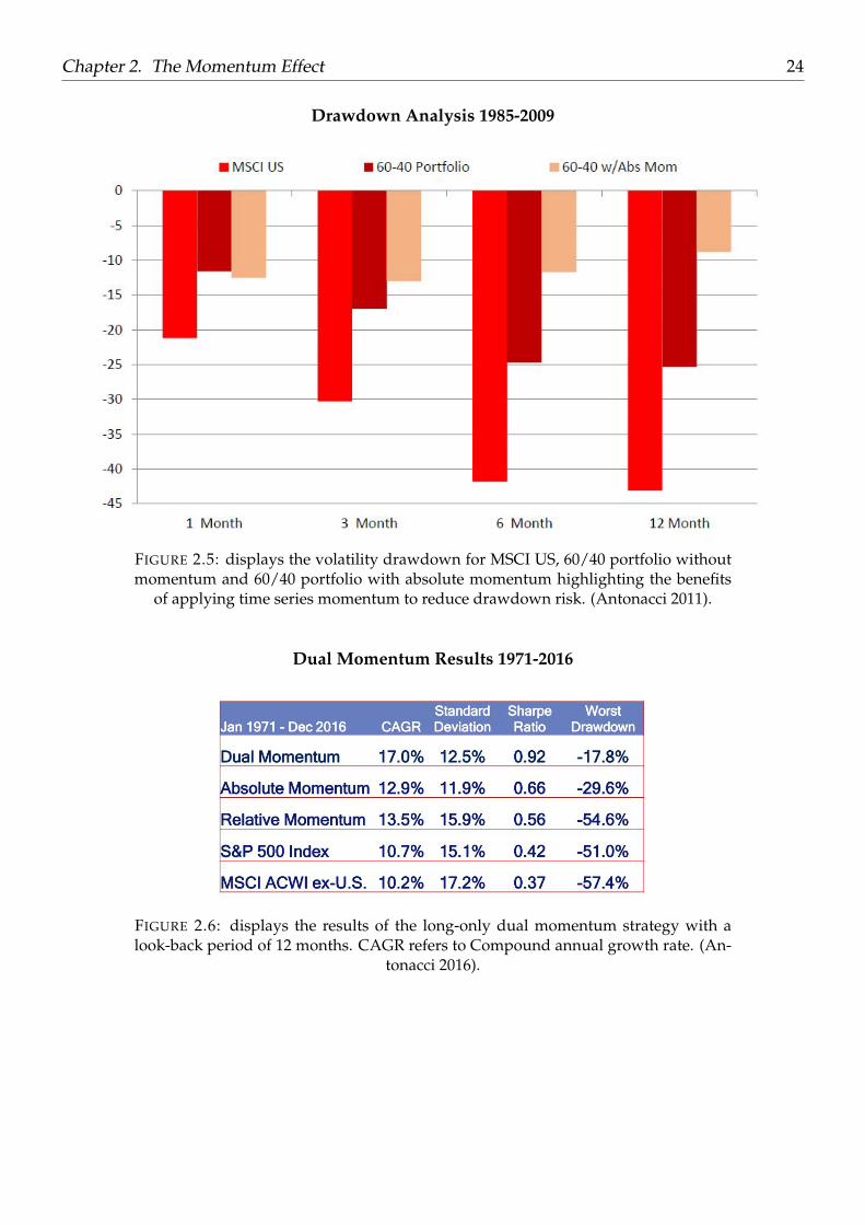
time for ACWI ex-US. Since momentum studies use either a six or a 12 months formation period,he selected the 12 months timeframe as the preferred look-back period for testing the strategy.Again in this analysis, Antonacci choose to rebalance positions monthly without skipping the lastmonth of observation.Declared results are supportive for the strategy since dual momentum shows the lowest draw-down (-17%) and the highest SR (0.92) with to respect to absolute and relative strategies in astand-alone application. Figure 2.7 shows the cumulative returns of the strategy and Figure 2.6displays a summary of the statistics. The use of dual momentum strategy makes diversificationmore efficient investing in assets only when they show both positive relative and absolute mo-mentum. Moreover, findings demonstrated that long momentum strategies worked extremelywell when considering a combination of absolute momentum and relative momentum and thattrend determination with absolute momentum can help mitigate downside risk and take advan-tage of regime persistence of the market, while both relative and absolute momentum can enhanceexpected returns.

Chapter 2. The Momentum Effect 20
Time Series Predictability Across All Asset Classes
FIGURE 2.1: Panel A and Panel B of display the results of the two-regression analysisdone by Pedersen & Moskowitz. They found that the past 12-month excess return ofeach instrument is a positive predictor of its future return, this time series momentumeffect persists for about a year and then partially reverses over the long horizons. Fig-ure 2.1 plots the t-statistics from the pooled regressions by month lag h. The positivet-statistics for the first 12 months (nine statistically significant) indicate strong returncontinuation or trend. The negative signs for the longer horizons indicate reversals,the most significant of which occur in the year immediately following the positive
trend. (Pedersen and Moskowitz 2011).

Chapter 2. The Momentum Effect 21
Cumulative Excess Return of Time Series Momentum and Diversified Passive Long Strate-gy,January 1985 to December 2009
FIGURE 2.2: plots the cumulative excess return of the time series strategy for all fu-tures contracts they have examined (on a log scale) compared to a passive long expo-sure for all instruments. To improve comparability, all the contracts are scaled by the
same conditional volatility. (Pedersen and Moskowitz 2011).

Chapter 2. The Momentum Effect 22
Best Formation Periods 1974-2012
FIGURE 2.3: displays the results of the clustering process of formation periods fordifferent assets. The highest Sharpe ratios for each asset is the one associated to thecluster of 12 months, then highest occurrences (8) are associated with a 12 months
formation period (Antonacci 2011).

Chapter 2. The Momentum Effect 23
60/40 Balanced Portfolios 1974-2012
FIGURE 2.4: displays the cumulative results of the long-only 12-month absolute mo-mentum strategy applied to a 60/40 portfolio compared with a 60/40 portfolio with-
out momentum (Antonacci 2011).
Chapter 2. The Momentum Effect 24
Drawdown Analysis 1985-2009
FIGURE 2.5: displays the volatility drawdown for MSCI US, 60/40 portfolio withoutmomentum and 60/40 portfolio with absolute momentum highlighting the benefits
of applying time series momentum to reduce drawdown risk. (Antonacci 2011).
Dual Momentum Results 1971-2016
FIGURE 2.6: displays the results of the long-only dual momentum strategy with alook-back period of 12 months. CAGR refers to Compound annual growth rate. (An-
tonacci 2016).

Chapter 2. The Momentum Effect 25
Cumulative Returns of the Dual Momentum strategy
FIGURE 2.7: displays the cumulative returns on a log scale of the strategy comparedwith the singular use of absolute and relative momentum and with long passive ex-
posures on S&P 500 and MSCI ex-US. (Antonacci 2016).

Chapter 2. The Momentum Effect 26
2.5 The Momentum Effect: A practical application
In this section, we want to prove the Momentum Effect through time series analysis leaving thecross-sectional application aside for the moment. In particular, we have replicated some ideasof applications and methodologies described by Pedersen & Moskowitz and Gary Antonacci intheir studies.
2.5.1 Data and Methodology
Our dataset is composed of equity monthly returns that include dividends and interest with aformation period of approximately 20 years (from December 1998 to July 2018). We have selectedthe most representative equity indexes regarding the Eurozone: DAX, IBEX, CAC, AEX, FTSE,and UK. All the data are taken using a Bloomberg terminal post. The results are obtained usingMATLAB.
2.5.2 Sharpe Evaluation on Formation Periods
The first step is to use a measure of performance such as the Sharpe ratio to find the best forma-tion period (look-back period) within the dataset. Specifically, we divide the time series of returnsinto different periods of time and we calculate the respective annualized SR for each period, thenwe classify each formation period using the SR as a unit of measure (highest SR for the best for-mation period).Following Gary Antonacci and his paper, the formation periods range from 2 to 18 months withan interval of 2 months. Results based on these settings show that the best cluster is at 12 monthsfollowed by 2, 14 and 16 months (Figure 2.8 and Figure 2.9 illustrate these findings). Many mo-mentum research papers use a 12-months formation period as a benchmark strategy for researchpurposes reducing transaction costs and data snooping.Figure 2.8 shows the same result in a more detailed way (it describes the best and the worstperformer), while Figure 2.9 is made by averaging all the indexes. Comparing to the analysisproduced by Gary Antonacci16 (he used an extended and different dataset), in our results thereare no significant levels17 in the cases of 18, 10, 8, and 6 months. This suggests using formationperiods that are close to 12-months or 2-months for a better performing application.Since our findings suggested to focus on a 2-months and on a 12 months look-back period, wewent deeper into the question producing another analysis and looking to the neighborhood of
16Antonacci, 201217The Sharpe ratio calculated over these formation periods (6, 8, 10, 18 months) is relatively low comparing to the
one of 12 and 2 months.

Chapter 2. The Momentum Effect 27
such critical windows. Results were interesting: we found that the highest level of SR is the oneassociated with formation periods of only one month (Figure 2.10). This strongly rejects the ideathat a 12 months look-back period needs to be preferred among all windows of observations andreminds to the fact that preferences need to be determined empirically in every case since theymay vary among instruments and across time.
Best Formation Periods
FIGURE 2.8: displays the results of the clustering process of formation periods fordifferent assets. The highest Sharpe ratios for each asset is the one associated to the
cluster of 12 months followed by 2, 16 and 14 months.

Chapter 2. The Momentum Effect 28
Best Formation Periods
FIGURE 2.9: displays the results of the clustering process of formation periods fordifferent assets. The highest Sharpe ratios for each asset is the one associated to thecluster of 12 months. The equity index is the arithmetic mean of all the index within
the dataset.

Chapter 2. The Momentum Effect 29
The Best Formation Period
FIGURE 2.10: displays the results of the clustering process of formation periods fordifferent assets. Expanding the window of the analysis the highest Sharpe ratio foreach asset is the one associated to the cluster of one month. This strongly rejects theidea that a 12 months look-back period needs to be preferred among all windows of
observations.

Chapter 2. The Momentum Effect 30
2.5.3 Volatility Model
The second step is to examine the time series predictability of returns across different time hori-zons using regression and volatility weighting. Practically, we proved the momentum effect bylooking at the time series of excess returns and at the auto-covariance between the security’s ex-cess return next month and its lagged 1-year return. If this autocovariance is positive, it meansthat the asset future excess returns are explained by the past and then profitable trading strategiescould be applied.In order to make meaningful comparisons across assets, all returns are scaled by their ex-ante orconditional volatility which it is calculated over the selected period of analysis18. This stage isfundamental since volatility varies across assets and across time. The volatility model is appliedto all the dataset and to ensure no look-ahead bias, the volatility estimates are at time t-1 ap-plied to time t returns. Differently from Pedersen and Moskowitz, we have estimated the ex-antevolatility for each asset with a simple univariate Garch (1,1). This choice has been made for sim-plicity reasons since the authors in their paper elaborate a more complex model of estimation. Inorder to formulate good estimates for the conditional variances and find the best possible Garch-fit for the data, we needed to test first the fit of the model and then the autocorrelation functionof standardized residuals for each asset within the database. In doing so we estimate19 the modelusing the MLE20 on the return data and we test the fit looking at the conditional volatility (thestandard deviation of conditional variance) and at the serial correlation of standardized residuals.In other words, we are calculating standardized residuals and checking if they respect the typicalassumption of being independent and identically distributed, if they are IID21 it means that thereis no serial correlation and that the autocorrelation function is bounded on zero22 . We look at thestandardized residuals and at the squared standardized residuals23 analyzing their autocorrela-tion functions. We confirmed the good fit of the model for each asset within the database (Figure2.12 and 2.11 show the autocorrelation test and the qualitative fit of the conditional variance forthe first asset returns).We also tested the distribution of the standardized residuals with a Jarque-Bera Test24 . If thevolatility model (used to estimate conditional volatility) holds, then the standardized residualsshould have approximately a normal distribution and nearly 95% of them will be between -2 and+2 25 (where sigma is the standard deviation of the conditional volatility). Findings rejected the
18The conditional volatility is calculated over the selected time horizon, if we modify the period of analysis thevolatility needs to be recalculated.
19In the estimation function we chose t-distribution with 5DOF instead of normality in order to have an approxi-mately normal distribution for the standardized residuals and a better fit for the model
20The estimation function used Maximum likelihood estimator by default.21Independent and Identically Distributed.22This is very useful to show that we capture volatility in a correct way.23Are calculated dividing square returns over the conditional volatility.24In statistics, the Jarque–Bera test is a goodness-of-fit test of whether sample data have the skewness and kurtosis
matching a normal distribution, Wikipedia [Internet]. Available from: https://en.wikipedia.org/wiki/Jaque_Bera[Accessed 20 September 2018].
25Following the 68 95 99.7 rule.

Chapter 2. The Momentum Effect 31
null hypothesis when we tested normality of the standardized residuals using a Gaussian dis-tribution as the distribution parameter of the volatility model. Differently, when we choose aT-distribution with 5 degrees of freedom as the distribution parameter of the volatility model wegot better statistics. In this last case, results were supportive and confirmed that the distribution ofthe standardized residuals may be approximated to a normal distribution. The positive outcomeof the Jarque-Bera test confirmed the good fit of the model to the data.
The Qualitative Fit of The Conditional Volatility
FIGURE 2.11: displays the qualitative fit of the estimated model to the data usingGarch (1,1). This is a visual fit of the conditional volatility on the volatility of theindex. This result refers only to the FTSE data but has been done successfully for
every asset.

Chapter 2. The Momentum Effect 32
Autocorrelation Fit
FIGURE 2.12: displays the autocorrelation functions of the standardized residuals(Panel A) and of the squared standardized residuals (Panel B) showing in both caseszero serial correlation. The former is calculated dividing the excess return for theconditional volatility, while the latter is obtained using squared excess returns overthe conditional volatility. This result refers only to the FTSE data but has been done
successfully for every asset.
Chapter 2. The Momentum Effect 33
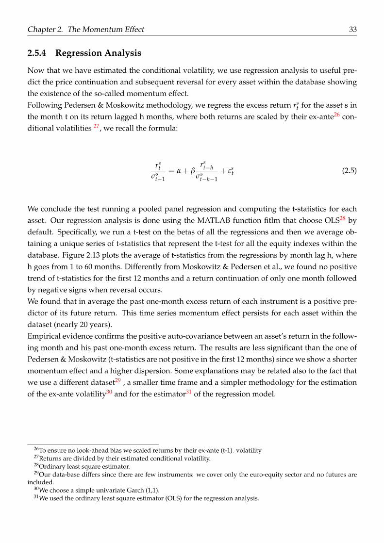
2.5.4 Regression Analysis
Now that we have estimated the conditional volatility, we use regression analysis to useful pre-dict the price continuation and subsequent reversal for every asset within the database showingthe existence of the so-called momentum effect.Following Pedersen & Moskowitz methodology, we regress the excess return rs
t for the asset s inthe month t on its return lagged h months, where both returns are scaled by their ex-ante26 con-ditional volatilities 27, we recall the formula:
rst
σst−1
= α + βrs
t−hσs
t−h−1+ εs
t (2.5)
We conclude the test running a pooled panel regression and computing the t-statistics for eachasset. Our regression analysis is done using the MATLAB function fitlm that choose OLS28 bydefault. Specifically, we run a t-test on the betas of all the regressions and then we average ob-taining a unique series of t-statistics that represent the t-test for all the equity indexes within thedatabase. Figure 2.13 plots the average of t-statistics from the regressions by month lag h, whereh goes from 1 to 60 months. Differently from Moskowitz & Pedersen et al., we found no positivetrend of t-statistics for the first 12 months and a return continuation of only one month followedby negative signs when reversal occurs.We found that in average the past one-month excess return of each instrument is a positive pre-dictor of its future return. This time series momentum effect persists for each asset within thedataset (nearly 20 years).Empirical evidence confirms the positive auto-covariance between an asset’s return in the follow-ing month and his past one-month excess return. The results are less significant than the one ofPedersen & Moskowitz (t-statistics are not positive in the first 12 months) since we show a shortermomentum effect and a higher dispersion. Some explanations may be related also to the fact thatwe use a different dataset29 , a smaller time frame and a simpler methodology for the estimationof the ex-ante volatility30 and for the estimator31 of the regression model.
26To ensure no look-ahead bias we scaled returns by their ex-ante (t-1). volatility27Returns are divided by their estimated conditional volatility.28Ordinary least square estimator.29Our data-base differs since there are few instruments: we cover only the euro-equity sector and no futures are
included.30We choose a simple univariate Garch (1,1).31We used the ordinary least square estimator (OLS) for the regression analysis.

Chapter 2. The Momentum Effect 34
The Momentum Effect
FIGURE 2.13: displays the results of our regression analysis plotting the average of thet-statistics of all the equity indexes. The positive significative trend of the t-statisticsfor the first month indicate a short return continuation. We found that in average thepast one-month excess return of each instrument is a positive predictor of its futurereturn. This time series momentum effect persists for all the dataset and the timehorizon (nearly 20 years) considered during the analysis. Finally, this result confirmsthat in our analysis a one-month look-back period needs to be preferred among allwindows of observations and reminds to the fact that these kinds of preferences need
to be determined empirically.

35
Chapter 3
Momentum Strategy
3.1 Data and Methodology
In this section, we want to test momentum trading creating a strategy that uses both absolute andrelative momentum at the same time1 .Our dataset is composed of equity monthly returns that include dividends and interest with aformation period of approximately 20 years (from December 1998 to July 2018). We have selectedthe most representative equity indexes regarding the Eurozone: DAX, IBEX, CAC, AEX, FTSE,and UK. All the data are taken using a Bloomberg terminal post. The results are obtained usingMATLAB and Python.
3.2 Backtesting
Since our analysis in chapter two strongly rejects the idea that a 12 months look-back periodneeds to be preferred among all windows of observations and reminds to the fact that preferencesneed to be determined empirically, to discuss the profitability of a strategy based on time seriesmomentum, we varied both the “look-back period” and the “holding period” on every instrumentwithin the dataset. Moreover, for each asset s and month t, we considered the excess return overthe past l months and depending on the sign of this excess return we hold the position for hmonths. Specifically, we recall the concept of formation and holding period periods as follows:
• Look-Back Period: it is the time considered for creating a signal. It is constructed creat-ing average functions of returns for each asset during l months. The signals are generated
1The effectiveness of a combined use of absolute and relative momentum has been studied by Antonacci in his pa-per, Gary Antonacci (2012), Risk Premia Harvesting Through Dual Momentum. Portfolio Management Consultants.

Chapter 3. Momentum Strategy 36
whether the excess return of these averages is positive or negative, in case of positive signalwe go long, while in case of negative signal we go short.
• Holding Period: it represents how long the position remains open and it varies from theparameter h.
Table 1, Table 2, Table 3, Table 4, Table 5 and Table 62 show the results of time series3 momen-tum backtested for each asset in case of positive signals4 (long positions). Table 7, Table 8, Table9, Table 10, Table 11 and Table 125 show the results of time series momentum backtested foreach asset in case of negative signals6 (short positions). These tables represent all the combina-tions of look-back periods and holding periods for every asset within the database over nearly 20years (1999-2018). Specifically defining li = look-back period (with i= 1,. . . ,12) and respectivelyhj = holding period (with j = 1,. . . ,17) we create 17 time series7 of monthly returns for each assetmoving from hj to li. Each table corresponds to a different instrument and indicates cumulativemonthly returns for every combination of (l, h).Moreover, we guarantee no overlapping of returns since we cumulate only returns that respectthe duration of the selected holding period. For example, if we consider FTSE (1,6) and we havea positive signal in the month of May, we will invest 1 euro in June and we will be able to rein-vest our capital only in December (6 months after) respecting the duration of the holding period,every other signal produced in the period between June and December will be treated as a newor separated investment (this process is automated for every asset and for every combination of l,h). Our findings differ from Pedersen & Moskowitz study suggesting most of the times the use ofa look-back period of one month. This is confirmed also by the results obtained with the Sharpeanalysis (in Chapter II) of the formation periods where the look-back period of one month presentthe highest value of SR. Finally, we compute the mean for all the tables of positive signals as wellas for all the tables of negative signals. These averages are represented in Figure 3.1.
2In the appendix.3Time series or absolute momentum is applied by buying or selling the asset when positive or negative signals
occur.4When the excess return calculated over the formation period is positive.5In the appendix.6When the excess return calculated over the formation period is negative.7This value depends on the max value of j.

Chapter 3. Momentum Strategy 37
Average of Backtested Results
FIGURE 3.1: shows the averages of the backtested cumulative returns of all the equityindexes (DAX CAC IBEX AEX and FTSE). Panel A illustrates the results in case of longpositions while panel B displays the results in case of short positions. Also in this case,the look-back period of one month is the one associated with higher returns confirm-ing that such time length window needs to be preferred in our analysis. Concerningthe holding period or the amount of time an asset is held, we pass from 14 in panelA to 17 in panel B. In general, the backtested results of long positions (panel A) aremore significative and present greatest differences in terms of returns than results ob-tained from short positions (panel B). Following our results, the best absolute strategyconsidering our equity indexes would be (1, 14) in case of long positions and (1, 17) incase of short positions. Conditional formatting has been made to highlight negativeand positive results: red color indicates negative or lower returns, while green colorindicates positive returns. In our calculations, there is no overlapping of observationsince every holding period is respected before considering the impact of the successive
investment.

Chapter 3. Momentum Strategy 38
3.3 Best Index Best Strategy Algorithm
The strategy can be summarized and automated with an algorithm8 that uses both cross-sectionalmomentum9 and times series momentum10. The former is used to switch between equity indexesand choose among them the “best index”. While the latter is used to switch between the previ-ously founded best index and bonds applying the “best strategy” in every possible case (Figure3.2). Since our results in the previous section confirmed the validity of formation periods of onemonth, we select this time horizon as the look-back period for the entire strategy.
Best Index and Best Strategy Algorithm
FIGURE 3.2: shows the Momentum Strategy and Illustrates with a graphical descrip-tion each action of the Best Index Best Strategy Algorithm. The numbers in red are the
steps of operation.
8The implementation is provisional, and it works only for t = 1.9We use cross sectional momentum to switch from equity index.
10We use absolute momentum to switch from “Best Index” to bond a and to find the “best period (l, h)”.

Chapter 3. Momentum Strategy 39
In order to better explain how the algorithm operates, we divide the procedure into differentsteps or moments:
• First step: Starting from the month t the algorithm collects the returns of every indexes s forthat month of observations and calculates their excess return11 rs
t .
• Second step: it looks at the absolute value of these excess returns “|rst |" and it selects the one
that has the higher absolute value “max |rst |”. The index associated with the highest excess
return (in absolute value) is called the “Best index”.
• Third step: it compares12 the excess return13 associated with the best index to the return ofa 3-month euro-government bond. If the excess return of the index is higher than the returnof the bond, it generates a positive signal otherwise a negative signal.
• Fourth step: If the signal is negative it invests in the bond if the signal is positive it looks atthe sign of the excess return and the bond is rejected.
Now in case the bond is rejected with a positive signal, the algorithm chooses to invest in the bestindex, but it needs to determine first the holding period of the investment. In order to find outhow long the asset needs to be held by the strategy, the algorithm simply looks at a table of ourbacktested long/short results14 . Then a new step must be followed:
• Fifth step: if the excess return associated with the best index s is positive, following theprevious step it must take a long position on s. In doing so it looks at the backtested-long15
results of the index s and selects the combination of (l, h) associated with the highest return.Since we set l = 1, it has to select only h respecting the value of l. If the excess returnassociated with the best index s is negative, this time must take a short position on s. Thenit looks at the backtested-short16 results of the index s and selects the combination of (l, h)associated with the highest return. Since we set l = 1, it has to select only h respecting thevalue of l.
The process described in the last step is called “Best strategy”.We repeat this procedure at the beginning of every month. These steps are recapped in Figure 3.2with a graphical description.
11These excess returns are obtained subtracting from returns the arithmetic mean of the past returns calculatedover the entire time series.
12It compares both negative and positive returns.13It is always considered the absolute value.14Grouped in the appendix.15Are the result backtested using long postions and presented in forms of tables in section 3.2.16Are the result backtested using short positions and presented in form of tables in section 3.2.

Chapter 3. Momentum Strategy 40
3.3.1 Test for t = 117 We use this test as an example since we retrace the steps discussed previously:
• First step: Starting from the month of June 2015, the algorithm collects the returns of theindexes within our dataset (DAX, CAC, AEX, FTSE, UK, and IBEX) for that month of obser-vations and calculates their excess return18 rs
t .
• Second step: the higher excess return in absolute value is the one associated with FTSE.Then it calls FTSE the “Best index”.
• Third step: it compares19 the excess return20 of FTSE to the return of a 3-month euro-government bond. FTSE has a 2% excess return while the bond has a return of 1% in June2018. Since |2%| is bigger than |1%|, it generates a positive signal.
• Fourth step: Since the signal is positive it looks at the sing of |2%|. 2% is positive so itmoves to the fifth step.
• Fifth step: it invests in FTSE taking a long position. In doing so it looks at Table 1 (FTSEfor long positions) and selects the combination of (l, 14). Then, it holds the position for 14months and call (1, 14) the “Best strategy”.
Thanks to the Best index Best strategy Algorithm we know that for June 2015, Best index is FTSEand the Best strategy is (1, 14): taking a long position for 14 months on FTSE. We repeat thisprocedure at the beginning of every month.The fifth step or the best strategy procedure is described in Figure 3.3 considering a long positionon the index FTSE.
17The test is made using a dataset of approximately 20 years (from 1999 to 2018).18These excess returns are obtained subtracting from returns the arithmetic mean of the past returns calculated
over the entire time series.19It compares both negative and positive returns.20It is always considered the absolute value.

Chapter 3. Momentum Strategy 41
Best Strategy of FTSE (1, 14)
FIGURE 3.3: displays the fifth step of the previous example using the results of FTSEbacktested for long positions (Table 1). This figure shows how the Algorithm givena look-back period of one month selects the holding period with the highest returnand finds the best strategy (1, 14). Using the Best index Best strategy algorithm we areable to apply the best strategy for each asset in every possible case. No matter in whatkind of frequency of operation we choose (months, days, minutes), the algorithm willgo long if momentum is positive, will go short when momentum is negative and willinvest in bonds in case of range bounded markets enhancing returns and ensuring the
best possible outcome for the entire strategy.

Chapter 3. Momentum Strategy 42
3.3.2 Modified Relative Momentum
In this application, we relax the concept of relative momentum using a light or modified versionof cross-sectional application where we don’t need to respect the condition of long/short match-ing or zero-net exposure. If we do not guarantee a zero-net exposure the relative strategy willsuffer from directional bias because we are creating negative or positive exposure. Then, not ad-justing positions for volatility will not be the primary cause of directional risk, since we alreadybearing that risk without guaranteeing the zero-net exposure. This allows us to simplify the pro-cedures and to not worry about adjusting positions and signals for volatility. Thus, to reduce thecomplexity of the overall strategy we believe that it is more convenient to apply modified relativemomentum and face directly the directional risk of the market.The modified cross-sectional momentum is seen as a comparison of performance among assetsthat belong to the same category (comparing between peers). In other words, to apply modifiedrelative momentum we don’t need to buy some assets (winners) and sell the same number ofassets (losers) but we only need to compare the performance of the instruments relative to theirpeers and choose the one that is outperforming (we create positive or negative net exposure). Forexample, considering two assets: X and Y. If X has outperformed Y by 2%, we say that X has apositive relative momentum effect with to respect to Y. In this application, we only consider thismodified version of cross-sectional momentum.
3.4 Results and Implementations
The algorithm has been tested only for the month of June 2015 and the results indicate the FTSEas the “best index” (with a positive signal) and the combination of look-back (1) and holding (14)as the “best strategy”. There is not complete backtesting of our strategy since the algorithm hasnot been fully completed.An interesting implementation of this algorithm would be to use this strategy in a pure high-frequency trading mode. Specifically, generating a risk premium algo-strategy by reducing thetime horizon of the estimation and shifting the time of the operations from months to minutes.It would be interesting to analyze the results (the differences in terms of “best index” and “beststrategy”) and the risk factor associated with. Another implementation would be the creation ofmodules to separate investments and instruments that belong to different asset class (i.e. equities-module, currencies-module, . . . etc.). The modules will protect the assets enhancing the diversifi-cation of the portfolio. In fact, the use of relative momentum over a big set of assets could cause aconstant drop out of some instruments that are less likely to be part of the winner-loser category(i.e. lagging assets that may suddenly start outperforming), this will be a possible cause of exclu-sion from the active portfolio. The use of relative momentum on modules could reduce this bias ofexclusion and guarantee a higher level of diversification over the entire strategy. Finally, in order

Chapter 3. Momentum Strategy 43
to protect the portfolio to large losses, it is necessary to set stop-losses or take-profit constraintsover the entire strategy21.
21There are many other useful and interesting implementations or studies such as drawdown exposure, expectedshortfall and payoff analysis that we do not cover in this dissertation.

44
Conclusion
Since 1993 momentum strategies were considered one of the most valuable techniques over theentire investment industry and have been subject of research of a great number of academic andprofessional studies. Alternative risk premia have changed the portfolio construction processshifting from a correlation diversification approach to a payoff diversification approach and be-coming the building blocks of multi-asset management. Statistical evidence suggested that manyfinancial assets show positive short-term autocorrelation or momentum bias22 and that trend fol-lowing strategies are profitable in almost every asset class. Moskowitz and Pedersen, as well asGary Antonacci, studied the trend following applications on equities, currencies, commodities,and bonds finding substantial abnormal returns, especially during extreme markets. Nowadaysevery informed investor should know the main benefits associated with the use of momentuminvesting and alternative risk premia. Nevertheless, it is highly important to continue to studysuch interesting properties elucidating the role of a wide use of ARP into a pre-crisis environment.The primary objective of this final thesis was not only to discuss ARP and to collect the existingliterature of momentum investing but also to prove the momentum effect and his profitabilitypresenting a simple strategy that uses eurozone data and applies automated absolute rules. Inthe second and third chapter, we replicate some methodologies and applications described byGary Antonacci and Moskowitz & Pedersen in their studies to prove the momentum effect23.The first step was to use a measure of performance such as the Sharpe ratio to find the best for-mation period (look-back period) within the dataset. Results indicated that the highest level ofSR was associated with formation periods of one month. Hence, we rejected the idea that a 12months look-back period needs to be preferred among all windows of observations and we re-minded to the fact that preferences need to be determined empirically in every case since theymay vary among instruments and across time.The second step was to examine the time series predictability of returns across different time hori-zons using regression and volatility weighting. Following Pedersen & Moskowitz methodology,we proved the momentum effect by looking at the time series of excess returns and at the auto-covariance between the security’s excess return next month and its lagged excess returns. In order
22Using the expression of momentum biases, we refer to the momentum effect that can be interpreted as ananomaly or as a bias of the market, behavioral theories.
23We refer to absolute momentum effect.

Chapter 3. Momentum Strategy 45
to make meaningful comparisons across assets, we scaled all returns by their ex-ante volatility.Once we tested the validity of the volatility model, we used regression analysis to useful predictthe price continuation and subsequent reversal for every asset within the database showing theexistence of the so-called momentum effect. Once again findings were supportive, and resultsconfirmed that in our analysis the look-back period of one-month needs to be preferred amongall windows of observations.Finally, in the last chapter, we tested momentum trading running a backtest and creating a strat-egy that uses both absolute and relative momentum at the same time24 . The strategy has beenautomated with an algorithm25 that uses cross-sectional momentum26 to choose the “best in-dex” and times series momentum27 to select and apply the “best strategy” in every possible case.The backtest proves that returns associated with formation periods of one month are the highestamong all assets within the database supporting results founded in the previous chapter. Thestrategy confirmed the validity of momentum investing showing the main benefits of mixingcross-sectional and time series momentum at an absolute level. In particular, such methods areinteresting to understand past performances and best asset combinations as well as further po-tential uses in high-frequency trading and portfolio construction.
24The effectiveness of a combined use of absolute and relative momentum has been studied by Antonacci in his pa-per, Gary Antonacci (2012), Risk Premia Harvesting Through Dual Momentum. Portfolio Management Consultants.
25The implementation is provisional, and it works only for t = 1.26We use cross sectional momentum to switch from equity index.27We use absolute momentum to switch from “Best Index” to bond a and to find the “best period (l, h)”.

46
Appendix
Results BacktestedIn this appendix, we show the results of Long and Short positions for the assets within thedatabase.The followings tables are the cumulative monthly returns of all the backtesting we using a timehorizon of nearly 20 years (1999-2018).
FTSE backtested for long positions
DAX backtested for long positions

Chapter 3. Momentum Strategy 47
UK backtested for long positions
IBEX backtested for long positions
AEX backtested for long positions
CAC backtested for long positions
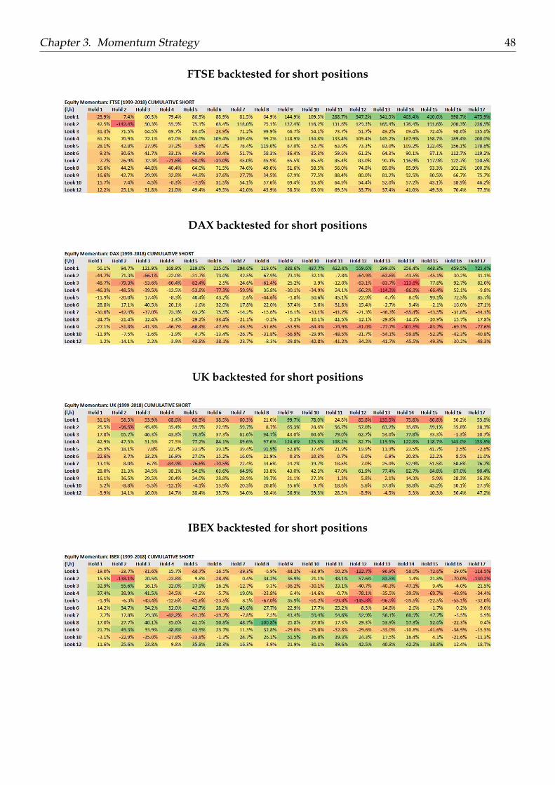
Chapter 3. Momentum Strategy 48
FTSE backtested for short positions
DAX backtested for short positions
UK backtested for short positions
IBEX backtested for short positions

Chapter 3. Momentum Strategy 49
AEX backtested for short positions
CAC backtested for short positions

50
Summary
Whether we decide to invest our savings or our time into a project, a new business opportunityor into something that seems to be appealing to us, we strongly believe that our choice will bepromising. When we do that we are betting, and every bet implies some risk. What we gather atthe end it’s the willingness to accept the risk, a premium.In Finance the risk premium it is defined as “the return in excess of the risk-free rate of return that aninvestment is expected to yield” 28. Maximizing this premium for a given level of risk it is alwaysbeen the principal objective of modern portfolio theory. It’s also well-known that Economics it’snot an exact science, but a social science and the word social means human, which in turn impliesirrationality, which again is the expression of our behavior. In recent years we filled this gap andwe start to move away from the traditional view of risk premium into a new one, the so-calledalternative risk premium.Traditional risk premia are returns that can be harvested passively from directional long expo-sures in asset classes such as stocks, bonds, commodities and so forth. By contrast, ARP 29 is adynamic and systematic source of return that behaves differently from those in traditional mar-kets 30 . While traditional risk premium includes factor investing 31 or smart beta strategies 32
that are related to systematic risk, the latter is structured as a long-short investment and it maybe independent of traditional risk premia. Moreover, ARP should not be confused with alphastrategies, which are believed to be driven by a manager’s security selection and market-timingskills. The ARP on traditional financial assets such as commodities, equity or currencies oftenresults from market behaviors and structured conditions of the market itself. If we start sellinglosers and buying winners, we are creating momentum. If we are betting on a cheap asset thathas potential growth and a higher fair price, we are considering value investing. If we think thatan asset yield is mispriced, we believe in carry opportunities.
28Risk Premium, Investopedia [Internet]. Available from:https://www.investopedia.com/terms/d/drawdown.asp[Accessed 20 September 2018]. Alternative Risk Premia.
29Alternative Risk Premia.30Communication department (2017), Alternative Risk Premia: What Do We Know? Viewpoint Amundi Asset
Management [Internet]. Available from: http://research-center.amundi.com/ [Accessed 20 September 2018].31Factor investing is an investment approach that involves targeting quantifiable firm characteristics
or “factors” that can explain differences in stock returns. Over the last 50 years, academic researchhas identified hundreds of factors that impact stock returns, Wikipedia [Internet]. Available from:https://en.wikipedia.org/wiki/Factor_investing [Accessed 20 September 2018].
32Smart beta investing combines the benefits of passive investing and the advantages of active investing strate-gies Investopedia [Internet]. Available from: https://www.investopedia.com/terms/d/smartbeta.asp [Accessed 20September 2018].

Chapter 3. Momentum Strategy 51
These are the most common sources of ARP and are also well-known for many years among in-vestors, the key difference is how they are implemented. In fact, if ARP strategies are includedin portfolios alongside traditional investments, they enhance diversification and provide benefits(e.g. reduce drawdown exposure 33 ) since they exhibit heterogeneous statistical properties.After the 2008 global financial crisis, the diversification has become the primary objective of insti-tutional investors and wealth funds who needed to restructure their portfolio in a low correlatedenvironment. To complicate the situation, it was also the uncertainty of future behavior of thestock-bond correlation that continues to be negative since the 90’s and should revert to positiveover the long run 34 . As a reaction wealth funds and sophisticated investors have switched fromcommon diversification procedures to a deleveraging equity solution using sovereign bond ashedging assets and corporate bond as lower beta assets (sovereign bonds are felt more as assetsfor hedging than for performance).ARP are expanding the universe of traditional risk premia and are becoming the building blocksof multi-asset management. In 2017, a survey from bFinance 35 suggests that ARP has beenthe area of the greatest interest among investors on a rolling 12-month basis. In the same year,Deutsche Bank reported some survey results 36 showing the growth of the percentage of investorswho allocate to ARP strategies, with an increase of 20% from 2015 the level has reached the 26 %in 2017. Furthermore, a recent Prime Brokerage survey 37 from Morgan Stanley reports that 79%of investors with more than $5 billion of assets under management in hedge fund investmentscurrently rely on ARP strategies or are considering to allocating on ARP.Since 1993 momentum strategies were considered one of the most valuable techniques over theentire investment industry and have been subject of research of a great number of academic andprofessional studies. Alternative risk premia have changed the portfolio construction processshifting from a correlation diversification approach to a payoff diversification approach and be-coming the building blocks of multi-asset management. Statistical evidence suggested that manyfinancial assets show positive short-term autocorrelation or momentum bias38 and that trend fol-lowing strategies are profitable in almost every asset class. Moskowitz and Pedersen, as well asGary Antonacci, studied the trend following applications on equities, currencies, commodities,and bonds finding substantial abnormal returns, especially during extreme markets. Nowadaysevery informed investor should know the main benefits associated with the use of momentuminvesting and alternative risk premia. Nevertheless, it is highly important to continue to studysuch interesting properties elucidating the role of a wide use of ARP into a pre-crisis environment.The primary objective of this final thesis was not only to discuss ARP and to collect the existing
33Drawdown, Investopedia [Internet]. Available from: https://www.investopedia.com/terms/d/drawdown.asp[Accessed 20 September 2018].
34If economic conditions and monetary policy permit this change.35“Manager Intelligence and Market Trends”, bFinance (February 2017).3615th Annual Alternative Investment Survey,” Deutsche Bank (March 2017).37“Recent Hedge Fund Trends,” Morgan Stanley Prime Brokerage-Strategic Content Group (July 2017).38Using the expression of momentum biases, we refer to the momentum effect that can be interpreted as an
anomaly or as a bias of the market, behavioral theories.

Chapter 3. Momentum Strategy 52
literature of momentum investing but also to prove the momentum effect and his profitabilitypresenting a simple strategy that uses eurozone data and applies automated absolute rules. Inthe second and third chapter, we replicate some methodologies and applications described byGary Antonacci and Moskowitz & Pedersen in their studies to prove the momentum effect39.The first step was to use a measure of performance such as the Sharpe ratio to find the best for-mation period (look-back period) within the dataset. Results indicated that the highest level ofSR was associated with formation periods of one month. Hence, we rejected the idea that a 12months look-back period needs to be preferred among all windows of observations and we re-minded to the fact that preferences need to be determined empirically in every case since theymay vary among instruments and across time.The second step was to examine the time series predictability of returns across different time hori-zons using regression and volatility weighting. Following Pedersen & Moskowitz methodology,we proved the momentum effect by looking at the time series of excess returns and at the auto-covariance between the security’s excess return next month and its lagged excess returns. In orderto make meaningful comparisons across assets, we scaled all returns by their ex-ante volatility.Once we tested the validity of the volatility model, we used regression analysis to useful predictthe price continuation and subsequent reversal for every asset within the database showing theexistence of the so-called momentum effect. Once again findings were supportive, and resultsconfirmed that in our analysis the look-back period of one-month needs to be preferred amongall windows of observations.Finally, in the last chapter, we tested momentum trading running a backtest and creating a strat-egy that uses both absolute and relative momentum at the same time40 . The strategy has beenautomated with an algorithm41 that uses cross-sectional momentum42 to choose the “best in-dex” and times series momentum43 to select and apply the “best strategy” in every possible case.The backtest proves that returns associated with formation periods of one month are the highestamong all assets within the database supporting results founded in the previous chapter. Thestrategy confirmed the validity of momentum investing showing the main benefits of mixingcross-sectional and time series momentum at an absolute level. In particular, such methods areinteresting to understand past performances and best asset combinations as well as further po-tential uses in high-frequency trading and portfolio construction.
39We refer to absolute momentum effect.40The effectiveness of a combined use of absolute and relative momentum has been studied by Antonacci in his pa-
per, Gary Antonacci (2012), Risk Premia Harvesting Through Dual Momentum. Portfolio Management Consultants.41The implementation is provisional, and it works only for t = 1.42We use cross sectional momentum to switch from equity index.43We use absolute momentum to switch from “Best Index” to bond a and to find the “best period (l, h)”.

53
Bibliography
Antonacci, Gary (2012). “Risk Premia Harvesting Through Dual Momentum. Portfolio Manage-ment Consultants”. In: Journal of Finance, pp. 15–20.
— (2013). “A Simple Rule-Based Strategy and Universal Trend-Following Overlay, Portfolio Man-agement Consultants”. In: Journal of Finance, pp. 15–20.
Bruder, B. and N. Gaussel (2011). “Risk-Return Analysis of Dynamic Investment Strategies”. In:Journal of Finance, 15–21.
Grinblatt M., Titman S. and R. Wermers (1995). “Momentum Investment Strategies, Portfolio Per-formance, and Herding: A Study of Mutual Fund Behavior”. In: American Economic Review,pp. 1088–1105.
Ilmanen, A. (2011). “Expected returns: An investor’s guide to harvesting market rewards. JohnWiley Sons”. In: Journal of Finance, pp. 397–450.
Jegadeesh, N. and S. Titman (1993). “Returns to Buying Winners and Selling Losers: Implicationsfor Stock Market Efficiency”. In: Journal of Finance, 65–91.
Moskowitz T.J., Ooi Y.H. and L.H. Pedersen (2012). “Time Series Momentum”. In: Journal of Finan-cial Economics, pp. 228–250.
Potters, M. and J-P Bouchaud (2006). “Trend Followers Lose More Often Than They Gai”. In:Wilmott Magazine, pp. 58–63.
Roncalli, T. (2017a). “Alternative Risk Premia: What Do We Know”. In: Journal of Finance, pp. 13–41.
— (2017b). “Understanding the Momentum Risk Premium: An In-Depth Journey Through Trend-Following Strategies”. In: Journal of Finance, pp. 1–102.