The Rise and Fall of Spatial Inequalities in France:A Long-Run Perspective∗

Pierre-Philippe Combes† Miren Lafourcade ‡

Jacques-Francois Thisse§ Jean-Claude Toutain¶

January 28, 2011

Abstract

This paper studies the evolution and determinants of spatial inequalities in France.To this end, we use a unique database providing data on value-added, employment,and population over the entire set of French “Departements” in 1860, 1896, 1930, 1982,and 2000. These data cover three sectors: Agriculture, Manufacturing, and Services.Firstly, we confirm the existence of a bell-shaped process of spatial concentration inManufacturing and Services over time. In contrast, labor productivity has been con-verging across departments. Secondly, we find considerable agglomeration economiesover the whole period. The spatial distribution of these gains is determined mainly bymarket potential in the first sub-period, 1860-1930, and higher education in the second,1930-2000.

JEL classification: N93, N94, O18, R12.Keywords: Economic geography, economic history, agglomeration economies, regionalproductivity, human capital.

∗We thank Claude Diebolt and Alexandre Kych (CMH-ADISP) for crucial help in collecting the human-capital data. We are also grateful to Tim Leuning and two anonymous referees for constructive suggestions,and to Vianney Brandicourt, Paul Cheshire, Andrew Clark, Paul Hohenberg, Philip Hoffman, Sandra Poncetand seminar participants at the NARSC conference in New York, the Atelier Francois Simiand (PSE), Collegede France, CESAER (Dijon), Katholiek Universiteit Leuven, and the Universities of Cergy-Pontoise, Lille I,Nantes, Paris II and Paris-Sud XI for helpful remarks.†GREQAM-Aix-Marseille Universite, Paris School of Economics (PSE) and CEPR; ppcombes@univmed.fr;

http://www.vcharite.univ-mrs.fr/pp/combes/. The support of the CNRS is gratefully acknowledged.‡ADIS-Universite Paris-Sud 11 and PSE; lafourcade@pse.ens.fr; http://www.pse.ens.fr/lafourcade/.§CORE-Universite catholique de Louvain, PSE and CEPR; jacques.thisse@uclouvain.be.¶Universite de Paris I-Pantheon-Sorbonne and ERMES-Universite de Paris II-Pantheon-Assas;

toutain.jean-claude@neuf.fr.

1 Introduction

What makes some countries rich and others poor has gained center stage in economicsand history. By way of comparison, little attention has been paid to the reasons why someregions, or other sub-national entities, are rich and others not. However, even today, re-gional disparities are at the root of considerable tensions between different political bodiesand jurisdictions in various countries, such as Belgium, Italy, Spain, and Russia.

That Paris is an oversized city growing at the expense of the rest of the country is oneof the most enduring urban legends in France. With the creation of the “Delegation al’Amenagement du Territoire et a l’Action Regionale” (DATAR) in 1963, French author-ities embarked upon various decentralization policies all of which were aimed at relo-cating firms and jobs away from Paris (Merlin, 2010). From 1962 to 1970, the objectivewas to boost the development of medium-sized cities (the “metropoles d’equilibre”), andafter 1970, the target shifted to supporting smaller cities (the “villes moyennes”). Morerecently, based on the English experience of new towns, the French government has fos-tered the development of “villes nouvelles”, which aim to attract the population of largecities to satellite towns via the supply of a broad portfolio of public facilities. This cornu-copia of policies shows how deeply-rooted the idea is that the French economy is spatiallyunbalanced.

This paper shows that the cliche “Paris et le desert francais” is to a large extent ground-less. In particular, our analysis reveals that the French economic space has followed abell-shaped process, with a phase of agglomeration of activities sparked by interregionalintegration, followed later on by a dispersion phase. As illustrated by the resilience ofthe French urban system (Eaton and Eckstein, 1997), this unfolding of economic activitiesdeveloped at a slow pace. The explanation of the main trends characterizing the evolutionof spatial inequalities in France thus requires long-run historical data, such as those usedin this paper.

To this end, we are privy to three different variables (value-added, employment, andpopulation) for three basic sectors (Agriculture, Manufacturing, and Services) at differenthistorical points in time (1860, 1896, 1930, 1982 and 2000), and at a fine geographical level,Departements.1 Working with three aggregate sectors is not as restrictive as it at first mightseem. Indeed, with such a long time-span, very few industries are present over the entireperiod (e.g. the automobile and computer industries are not). The period 1860-2000 sawa number of dramatic changes in French economic structure: the steady fall in transportcosts brought about by the birth of the railroads and the development of a dense net-work of roads and highways, the rise of Manufacturing, the expansion of Services and themechanization of Agriculture, the “Trente Glorieuses,” 2 the growth of the Welfare State,the process of European integration, a recent move towards de-industrialization, and thebirth of new information and communication technologies. This non-exhaustive list isenough to portend fundamental changes in the geography of economic activity, even at avery aggregated sectoral level.

1The division of France into “Departements” was adopted in 1790 during the French Revolution. Thesewere designed to replace the old “provinces”, which displayed significant variation in terms of tax systems,population and land areas. By way of contrast, the new jurisdictions aimed to create more homogeneous andregular spatial units under a common central legislation and administration. Their size was chosen so thatindividuals from any point in the department could make the round trip by horse to the capital city in nomore than two days, which translated into a radius of 30 to 40 km. Initially, France included 83 departments,the number of which has gradually been increased to 100 (94 in Mainland France, which does not includeCorsica and overseas departments and territories). This allows us to work with a definition of departmentsthat is consistent over time.

2This refers to the thirty-year period of rapid growth that has followed the end of World War II in France.

1

Our analysis reveals the existence of a bell-shaped curve for both Manufacturing andServices: the spatial concentration of these sectors first increased from 1860 to 1930, andthen fell thereafter. The spatial concentration of Agriculture has slightly increased overtime, but this sector remains the least concentrated. By way of contrast, labor productivityhas converged across departments from 1860 to 2000. In other words, spatial inequalitiesin primary incomes have steadily decreased. As the bell-shaped curve is one of the keypredictions of new economic geography, we thus find it natural to appeal to the analyticaltool-kit of this field to uncover the main forces that have shaped the French economicspace. In doing so, we hope to show that the French experience can shed light on whathas happened, and may happen, in many other countries.

The first force shaping the location of economic activity refers to the size of the localmarket and the intensity of local interactions. This is typically captured by local employ-ment density. Second, the concentration of firms in the same industry is conducive to therapid imitation and diffusion of innovation and new production processes, as well as thesharing of specific inputs, thereby creating gains from specialization. However, increasingspatial concentration within the same industry also intensifies labor- and product-marketcompetition, encouraging firm dispersion. The third force refers to the potential benefitsof locating in a diversified range of industries. Radical innovations developed in one in-dustry may then be implemented in other industries, producing significant productivitygains. Sectoral diversity also protects against industry-specific negative shocks by diver-sifying the local industrial structure. Glaeser et al. (1992) suggest that these gains fromdiversity are the driving force behind the agglomeration of economic activity. On the con-trary, Henderson et al. (1995) put more weight on the role of specialization in the rise ofsuccessful clusters.3 Our analysis confirms the existence of density economies for Manu-facturing and Services, while there are diseconomies in Agriculture. Specialization has apositive effect in Services, but a negative effect in Agriculture. Finally, gains from diversityare also observed in general.

Two additional factors help to shape the economic space. Given the role of transportcosts in economic geography, we expect firms’ proximity to large outlets to increase prof-its. We here follow the recent literature (Head and Mayer, 2004; Redding and Venables,2004; Redding and Sturm, 2008) and assess the impact of market potential on spatial in-equalities. This variable provides a simple, but meaningful, measure of the accessibilityof a department to the rest of the country. We do indeed find departmental market po-tential to be positively correlated with firm productivity in 1860 and 1930, that is, whentransport costs were relatively high in France.4 However, the subsequent spectacular de-cline in transport costs, greater openness to international trade, and growth of knowledge-intensive activities, saw departmental-market potential overshadowed by local educationlevels by 2000.

While the positive effect of education on growth is well known at the national level,more recent work has underlined the role of education in structuring the spatial distri-bution of economic activity (Moretti, 2004; Combes et al., 2008a). Skilled workers andskill-intensive firms tend to cluster together to benefit from technology or informationspillovers, as well as better matches between jobs and workers (Duranton and Puga, 2004).Although human capital contributed to average labor productivity between 1860 and 1930,

3Our consideration of only three aggregate sectors reduces our scope for the interpretation of these exter-nalities. Knowledge spillovers may well not apply at such an aggregated level. However, other externalities(sharing intermediate inputs and local public goods, as well as labor-pooling effects) likely remain relevanteven at the three-sector level.

4This is in line with Tirado et al. (2002) and Wolf (2007), who also find that the market potential is a majordeterminant of industry location in Spain (in 1856 and 1893) and Poland (over 1925-1937) respectively. Section2 provides some other references.

2

it was not conducive to agglomeration economics. This likely reflects France’s widespreadand fairly homogenous elementary schooling system during this period. On the contrary,human capital has played a significant role in structuring France’s economic space in morerecent years. This is especially true of higher education, as the metropolization of the econ-omy has gone hand-in-hand with the clustering of high value-added activities in largeurban agglomerations, which thereby become more productive.

In what follows, we review the related literature, in order to ground our empiricalstrategy in modern economics (Section 2). We then analyze the aggregate (Section 3) andindustry-level (Section 4) spatial distribution of jobs and productivity. Last, we evaluatethe magnitude of agglomeration economies and the other determinants of the spatial de-velopment of economic activity (Section 5).

2 Lessons from new economic geography

The main thrust of new economic geography is that there exists a long swing in re-gional disparities, in which there is first a rise and then a fall in spatial inequalities causedby steadily falling transport costs.5 Tackling the shaping of the economic space fromthis angle is of relevance because the transport sector has undergone the most stunningchanges since the beginning of the Industrial Revolution. According to Bairoch (1997,chapter IX, our translation), “between 1800 and 1910, it can be estimated that the lower-ing of the real average prices of transportation was of the order of 10 to 1”. Transportcosts continued to fall after World War I. For example, in the United States, Glaeser andKohlhase (2004) note that over the Twentieth Century, the costs of moving manufacturedgoods have declined by over 90% in real terms. In France, freight rates by ton-kilometerfell by 36% between 1841 and 1851, and by 19% between 1851 and 1869 (Caron, 1997,p.556). Even during the recent 1978-1998 period, road transport costs fell by 38% (Combesand Lafourcade, 2005).6

Given such dramatic decreases in transport costs, we think that it is reasonable to be-lieve that the French economy has navigated through the whole of the bell-curve high-lighted by new economic geography (Fujita et al., 1999; Combes et al., 2008b). In brief,when transport costs are high, economic activity is scattered throughout the area. Astransport costs fall, firms’ proximity to natural resources and local outlets matters less.Hence, firms operating under increasing returns find it more profitable to cluster closeto the largest markets in order to better exploit scale economies (this is especially true ofmanufacturing firms). Lower transport costs make the supply of peripheral areas less ex-pensive, leading these areas to lose a significant share of their industries. The setting-upof new firms and the launching of new industries in a given region go hand-in-hand withthe geographic concentration of the labor force, leading in turn to an increase in demandfrom the arrival of these new consumers and producers.

The increasing size of the local labor and goods markets makes these regions evenmore attractive for both firms and workers, producing a self-reinforcing agglomerationprocess for both labor and industrial and ancillary activities. Conversely, decreasing- orconstant-returns-to-scale sectors remain to a large extent dispersed (which is the case forAgriculture), or mirror the movements in the spatial distribution of population (as forServices). Nevertheless, the agglomeration of firms and workers produces new costs as-sociated with land use (higher rents, commuting costs and wage rates, and the congestion

5New economic geography can thus be argued to provide a solid micro-economic underpinning to theideas developed much earlier by Williamson (1965).

6It is worth noting that these falls are not only caused by innovations in transportation technology andinfrastructure improvements, but also by changes in transport competition regimes.

3

of local transport networks), which make larger markets less attractive. With continuingfalls in freight costs, we may see the gradual unraveling of agglomeration: manufacturingindustries and the corresponding business-to-business services gradually relocate to theperiphery. The development of spatial inequality is therefore bell-shaped. The initial re-duction in transport costs leads to greater spatial concentration, but beyond a certain pointfurther falls yield re-dispersed economic activity. Land-intensive industries are likely tobe the first to move to the outskirts of large cities or peripheral areas to benefit from lowerland rents.

Most countries exhibit, both now and in the past, considerable regional disparities,the evolution of which is difficult to assess because of the lack of trustworthy historicaldatasets. As only relatively few historical analyses have appealed to the tools and conceptsof economic geography, it may be useful to summarize their main findings. Kim (1995)can be viewed as a precursor in this field. Computing Gini indices for twenty Americanindustries in 1860, 1914, 1947, 1967, and 1987, he finds a bell-shaped relationship betweeneconomic integration and geographical concentration in the manufacturing sector. Kimand Margo (2004) suggest that both regional specialization and spatial income inequalitiesin the US reached their peak early in the Twentieth Century. In particular, focusing on nineUS macro-regions, Kim (1998) finds that regional specialization in Manufacturing rosesubstantially after 1890, flattened out during the interwar years, and then fell substantiallythrough 1987 to the point where Manufacturing was more dispersed than in 1860. By wayof contrast, in Services, economic integration led to regional despecialization.

Dividing Spain into eight macro-regions, Roses (2003) observes that the most dynamicindustrial sectors became more concentrated over the Nineteenth Century, when Span-ish regions started to come together to form an integrated national economy. Paluzie etal. (2004) and Roses et al. (2010) extend this analysis and confirm the bell-shaped relation-ship for Spain, with widening disparities being caused by the very uneven distribution ofManufacturing and Services. The turning point of this curve occurred after the interna-tional integration of the Spanish economy in the mid-1970s.

Though covering a much shorter period, the European Union is another useful bench-mark to test the bell-shaped curve due to the high pace of integration. Using semi-parametricestimation techniques and NUTS2 regional data for a panel of twelve European countriesof the EU-15, Barrios and Strobl (2009) find strong support for the bell-shaped curve overthe 1975-2000 period. Our analysis thus concurs with existing work by concluding for aninverted U-shaped curve in France. We should stress, however, that it is conducted at amuch finer spatial level than in the papers mentioned above.

Starting from the work of Kuznets, a vast literature has highlighted a similar invertedU-shaped pattern of inequality across individuals (Morrisson, 2000). Since labor produc-tivity can be viewed as a rough proxy for the average individual income in each depart-ment, it is worth comparing our results to those found in this literature. According toPiketty et al. (2006), individual inequality increased during the 1860-1913 period and fellafter 1913, both in Paris and the rest of France. The initial concentration of wealth wasdriven by the growth of large industrial and financial businesses, while declining inequal-ity occurred because of major adverse shocks such as World Wars I-II and the Great De-pression. This is to be contrasted with the convergence of labor productivity found here,which would rather support the hypothesis that an increasing number of workers movingto high-paying sectors has triggered a continuous decline in primary income inequality.

4

3 Spatial aggregate dynamics

Our analysis relies heavily on the work of Toutain, who constructed measures of pop-ulation, employment, and value-added for each French department in 1860, 1896 and 1930(see Appendix, Tables A.1, A.2 and A.3). As these data have not been published to date,the Appendix describes the sources and methods used in their construction. We restrict thepresentation to 1860 and 1930 data only, because the method used for 1896 is the same asfor 1860 except for Manufacturing for which, unfortunately, the value-added is not avail-able in 1896. The 1982 and 2000 data on population, employment and value-added comefrom the EUROSTAT database.7

3.1 National trends

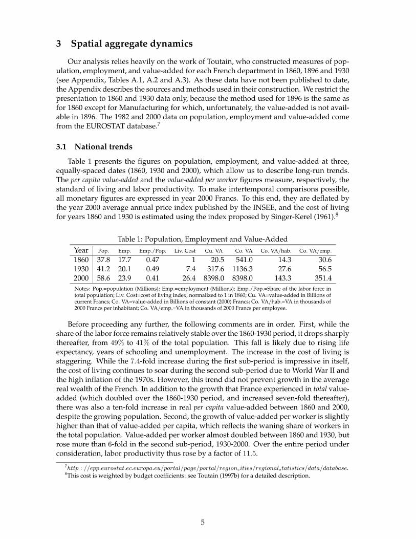
Table 1 presents the figures on population, employment, and value-added at three,equally-spaced dates (1860, 1930 and 2000), which allow us to describe long-run trends.The per capita value-added and the value-added per worker figures measure, respectively, thestandard of living and labor productivity. To make intertemporal comparisons possible,all monetary figures are expressed in year 2000 Francs. To this end, they are deflated bythe year 2000 average annual price index published by the INSEE, and the cost of livingfor years 1860 and 1930 is estimated using the index proposed by Singer-Kerel (1961).8

Table 1: Population, Employment and Value-AddedYear Pop. Emp. Emp./Pop. Liv. Cost Cu. VA Co. VA Co. VA/hab. Co. VA/emp.

1860 37.8 17.7 0.47 1 20.5 541.0 14.3 30.61930 41.2 20.1 0.49 7.4 317.6 1136.3 27.6 56.52000 58.6 23.9 0.41 26.4 8398.0 8398.0 143.3 351.4Notes: Pop.=population (Millions); Emp.=employment (Millions); Emp./Pop.=Share of the labor force intotal population; Liv. Cost=cost of living index, normalized to 1 in 1860; Cu. VA=value-added in Billions ofcurrent Francs; Co. VA=value-added in Billions of constant (2000) Francs; Co. VA/hab.=VA in thousands of2000 Francs per inhabitant; Co. VA/emp.=VA in thousands of 2000 Francs per employee.

Before proceeding any further, the following comments are in order. First, while theshare of the labor force remains relatively stable over the 1860-1930 period, it drops sharplythereafter, from 49% to 41% of the total population. This fall is likely due to rising lifeexpectancy, years of schooling and unemployment. The increase in the cost of living isstaggering. While the 7.4-fold increase during the first sub-period is impressive in itself,the cost of living continues to soar during the second sub-period due to World War II andthe high inflation of the 1970s. However, this trend did not prevent growth in the averagereal wealth of the French. In addition to the growth that France experienced in total value-added (which doubled over the 1860-1930 period, and increased seven-fold thereafter),there was also a ten-fold increase in real per capita value-added between 1860 and 2000,despite the growing population. Second, the growth of value-added per worker is slightlyhigher than that of value-added per capita, which reflects the waning share of workers inthe total population. Value-added per worker almost doubled between 1860 and 1930, butrose more than 6-fold in the second sub-period, 1930-2000. Over the entire period underconsideration, labor productivity thus rose by a factor of 11.5.

7http : //epp.eurostat.ec.europa.eu/portal/page/portal/regioncities/regionalstatistics/data/database.8This cost is weighted by budget coefficients: see Toutain (1997b) for a detailed description.

5

3.2 Local trends

Our analysis focuses on 87 departments in Mainland France. For today’s departmen-tal map to match up to the 1860 boundaries, we reconstruct the Seine department (whichtoday includes Paris, the Hauts-de-Seine, Seine-Saint-Denis, and Val de Marne) and thedepartment of Seine-et-Oise (which is now Essonne, Val d’Oise and Yvelines). In the samevein, we reunify the Haut-Rhin and the current Territoire-de-Belfort, which was not an-nexed to Germany in 1871, to produce the original Haut-Rhin. The 1871 French-Germantreaty also led to the annexation of a significant part of Meurthe and Moselle, with thenon-annexed parts of both joining together to form Meurthe-et-Moselle. To avoid any dis-crepancies, we thus created a “pseudo-department” by merging Meurthe and Moselle for1860, and Meurthe-et-Moselle and Moselle for subsequent years. Last, it should be keptin mind that the three French departments of Alsace-Lorraine (Bas-Rhin, Haut-Rhin andMoselle) were part of Germany from 1871 to 1918. Therefore, the number of observationsis slightly smaller in 1896 than in the other years.

We can appeal to a number of different tools to analyze the spatial distribution of eco-nomic activity. The Theil index (Theil, 1967) bears the advantage of allowing inequalityacross space to be captured at two nested geographical levels: Regions and Departments.9

More precisely, inter-departmental inequality can be decomposed into measures of con-centration within and between today’s 21 French continental regions. Moreover, we adopta definition of the Theil index which measures the difference between the actual distribu-tion of economic activity and the benchmark uniform distribution. Formally, for a givenactivity distributed across D departments, the Theil index is defined as follows:

T =D∑

d=1

Ad

Alog

Ad

A/D, (1)

where Ad is the level of activity in department d, while A =∑D

d=1Ad is the total levelof activity. The Theil index equals zero when the activity is uniformly distributed acrossdepartments: Ad = A/D for all d. At the opposite extreme, if all activity were to take placein only one department, the Theil index is logD = 1.94 (for D = 87). Intermediate valuesbetween the two capture varying degrees of spatial concentration: the higher is the Theilindex, the greater is the spatial concentration of economic activity.

As noted above, one attractive property of the Theil index is the way it allows observedinter-departmental inequality to be decomposed into its within-region (Tw) and between-region (Tb) components:

T = Tw + Tb.

The Tw-term captures the weighted average of Theil indices within region r, Tr:

Tw =R∑

r=1

Ar

ATr, (2)

where R is the number of regions, and Ar =∑Dr

d=1Ad the level of activity in region r ,which includes Dr departments. The Theil index for region r is given by the same expres-

9In 1956, departments were grouped together into 26 (21 continental) regions, in order to implement anumber of policies at a larger spatial scale.

6

sion as that for T , but now applied to the departments of which region r consists:

Tr =Dr∑d=1

Ad

Arlog

Ad

Ar/Dr. (3)

The Tb-term corresponds to the between-region Theil index:

Tb =R∑

r=1

Ar

Alog

Ar/Dr

A/D. (4)

Table 2 presents the results obtained for population, employment, and value-added.

Table 2: Theil indices for population, employment, and value-addedVariable Theil 1860 1896 1930 1982 2000Population Total 0.13 0.21 0.35 0.40 0.40

Between 0.07 0.12 0.22 0.26 0.26Within 0.06 0.09 0.13 0.14 0.14

Employment Total 0.13 0.24 0.38 0.50 0.50Between 0.07 0.14 0.22 0.32 0.33Within 0.07 0.09 0.15 0.19 0.17

Unoccupied Total 0.14 0.24 0.33 0.35 0.35Between 0.08 0.14 0.21 0.23 0.23Within 0.06 0.09 0.12 0.12 0.12

Value-Added Total 0.30 - 0.69 0.67 0.72Between 0.17 - 0.43 0.44 0.48Within 0.13 - 0.26 0.23 0.24

Notes: Total=total Theil-index; Within=intra-Regional Theil index; andBetween=inter-Regional Theil index. (ii) Value-added of Manufacturing is missingfor 1896, so that we cannot compute the corresponding Theil indices.

This reveals the substantial increase in the spatial concentration of the French population overthe course of the past 150 years, as illustrated by the three-fold increase in the total Theil indexbetween 1860 and 2000, with a stronger increase during the first sub-period. Over time,the population has become increasingly concentrated in a small number of departments(or perhaps even cities, but the data are not disaggregated enough for us to check thisconjecture). The spatial concentration of employment is even more pronounced, increas-ing dramatically over time. Yet, the Theil indices remain much lower than their maximalvalue (1.94), which does not lend credence to the famous “Paris and the French desert”.Note also that the concentration of unoccupied people stabilizes after 1930, which mayin part reflect an increasing number of individuals returning to their place of birth afterretirement. Last, although value-added is consistently more spatially unequal than othermeasures, its associated increase in concentration is less rapid than that of population andemployment.10

Over the whole time-period, spatial inequality is primarily due to the greater divergence ofregions. Between 1860 and 1930, the within- and between-region variations in both popu-

10Our results could be biased by the fact that French departments are of unequal size. We have, therefore,recomputed the Theil indices for all of our variables in density terms (variables expressed per square kilometerof land). They keep displaying the same pattern, with one notable exception: unlike the case for the absolutevalues, the pattern of concentration for population densities is bell-shaped. During the second sub-periodunder consideration, people have moved towards departments with greater land areas, probably because ofhigh land rents in urbanized departments having a small size.

7

lation and employment rise at more or less the same rate (the Theil indices fall just shortof tripling for both variables). The rise in spatial inequality in value-added is larger be-tween than within regions. Over the period 1930-2000, intra-regional inequality remainsremarkably stable. As a result, the observed increase in concentration is driven mainly byinter-regional variations. This suggests that a small number of French departments (re-gional capitals are the most likely candidates) have become progressively more attractive,to the detriment of the others whether or not they belong to the same region. Still, thewithin-Theil indices have also grown, thus showing that there is intra-regional inequality,even if they are well below their maximum values.11 Therefore, contrary to general beliefs,the French space-economy seems to be characterized by the emergence of multi-polarizationthrough the rise of second-tier urban regions.

Before proceeding, observe that the use of regions as an intermediate spatial scale is ad-mittedly arbitrary, as French regional boundaries were only drawn up after World War II.However, we believe that the Theil decomposition is useful and important for the follow-ing two reasons. First, we have just seen that the alleged phenomenon of “Paris et le desertfrancais” is not consistent with the data. Second, as described in Section 1, the concentra-tion of activity in the metropolitan area of Paris has given rise to various decentralizationpolicies aiming at relocating firms and jobs away from this area. Our results suggest thatthe policy of “metropoles d’equilibre” might have been successful since regional dispar-ities increased much less over 1930-2000. However, the growth of medium-sized citiesoccurred more through the stabilization of disparities within regions than through the re-location of activities away from Paris. Therefore, the Theil index allows us to show that thedecentralization policies of “villes moyennes” and “villes nouvelles” did not fully deliverthe expected outcome.

Table 3: Theil indices for value-added per capita and per employeeVariable Theil 1860 1930 1982 2000Value-Added/capita Total 0.039 0.025 0.015 0.017

Between 0.020 0.011 0.007 0.007Within 0.019 0.014 0.008 0.010

Value-Added/emp. Total 0.055 0.029 0.009 0.007Between 0.035 0.016 0.006 0.003Within 0.020 0.013 0.004 0.004

Notes: Total=total Theil index; within=intra-Regional Theil index; Between=inter-Regional Theil index; and Value-Added/Empl.=value-added per employee.

In contrast to total value-added, both per capita value-added and the average produc-tivity of labor have spread among French regions as well as among the departments thatmake up each region (see Table 3). In addition, the latter exhibits even greater dispersionover time than the former. Overall, the spatial inequality of productivity has fallen, ex-hibiting a five-fold decline over the course of 140 years. As a result, alongside the increasein the spatial concentration of population and production, we observe a fall in labor-productivityinequality across departments. It is worth noting that changes in spatial inequality come pri-marily from the between-regions evolutions. However, unlike for total value-added andemployment, they lead to convergence.

Although economic geography does not have much to say about the spatial distribu-tion of individual incomes, these contrasting developments over time can be explained in

11Since the smallest number of departments by region is 2 and the largest 8, the maximum value islog(D/Dr) = log(87/2) = 1.64 for the between-Theil index, and logDr = log8 = 0.90 for the within-Theilindex.

8

the following two ways. First, it seems reasonable to believe that the substantial increase inthe number of public-sector jobs has contributed to the convergence in standards of livingacross the country. Government spending as a percentage of GDP grew from 3% in 1860 to6% in 1930 (Fontvieille, 1976, 1982), while the ratio of public-sector jobs to the total laborforce rose from 4.4% to 6.2%. In 2000, the corresponding figures were 51.6% and 25.7%,respectively. Public employment was thus unlikely to have played a major role in the evo-lution of the service sector during the first sub-period. In contrast, the growth of the publicsector during the second sub-period was spectacular. To a large extent, this corresponds tothe creation of jobs triggered by the spread of educational and health facilities, the exten-sion of universal services, and other decentralization policies. These types of services areof a business-to-consumer nature and are tied to the local population. This could explainwhy Services became more concentrated than Manufacturing over the second sub-period,as will be seen below.

Furthermore, given that workers tend to migrate towards areas offering higher wages,it follows that the wage gap between regions should decrease, ceteris paribus. However,“everything else equal” rarely holds: economic activity is redistributed across industries,which naturally gives firms incentives to change location. The French work force actuallyexperienced a greater rise in concentration than that for value-added, especially between1860 and 1930 (see Table 2). Economic geography suggests that spatial concentration ismore pronounced in those industries that are characterized by scale economies, with theother sectors remaining more dispersed. In this context, migration occurs along both thespatial and sectoral dimensions which, from a theoretical standpoint, favors an equaliza-tion of wages across space, which is confirmed here in the convergence of labor productiv-ity. Conversely, the law of diminishing returns makes the agricultural regions that theseworkers left more productive. As a result, more concentrated departments exhibit slowerlabor productivity growth, while the increasingly labor-depleted departments effectivelycatch-up in labor-productivity terms.

It is important to emphasize that the fall in the spatial inequality of labor productivity doesnot reflect the dispersion of economic activity, as a small number of departments are home toan increasing share of total value-added over time. Somewhat paradoxically, the greaterequality of productivity is triggered by the concentration of increasing-returns activities.The maps presented in the next section provide empirical support for this hypothesis.

3.3 A cartographic illustration

Figure 1 maps the departmental distribution of per capita value-added as a percentageof the national average: (V Ad/Popd)/(V A/Pop). The six categories are determined by theautomatic allocation of the 1860 data,12 which are retained for 1930 and 2000.

Wealth disparities across departments vary by a factor of 1 to 4. The two highest percapita value-added classes include 16 departments in 1860, but only three in 1930 andtwo in 2000. Over time, the Northern departments of France lose their leading position:Seine (Paris) and Rhone (Lyon) are the only two departments which remain in the top twocategories over the whole period.13

Not surprisingly, Parisians are twice as rich as the national average, while Rhone in-habitants, though less affluent, have a per capita income which is 30% above the nationalaverage. At the other end of the spectrum, six departments (Ardeche, Ariege, Lozere, Can-tal, Lot and Cotes du Nord) are in the sixth and lowest category over the entire period.

12Precisely, classes are defined in such a way as to minimize the sum of their class-specific variances.13French Departments are named in the Appendix, Figure A.1.

9

Figu

re1:

Dep

artm

enta

lval

ue-a

dded

per

capi

ta(%

ofth

eco

untr

yva

lue-

adde

dpe

rca

pita

)

Figu

re2:

Dep

artm

enta

lval

ue-a

dded

inM

anuf

actu

ring

(%of

the

coun

try

valu

e-ad

ded

inM

anuf

actu

ring

)

10

These departments represent approximately one quarter of all departments in the low-est category; the least successful department has a standard of living of half of the nationalaverage. Apart from these very few departments that maintain their positions at the tailsof the distribution, the remaining departments experience a certain degree of mobility,which may account for the income convergence noted above. Haute-Garonne, and theblock formed by Isere, Haute-Savoie and Savoie have seen their standard of living growregularly, with the two latter departments experiencing gains substantial enough to catch-up to the national average in 2000. On the other hand, Ardennes, Calvados, Herault, andSeine-et-Marne have been the main losers in the wake of France’s spatial restructuring,falling from the first to the last two categories. There is also a marked decline on the At-lantic coastline, apart from Seine-Maritime and Gironde. Finally, a last category of depart-ments do not exhibit much variability over the entire period (e.g. Pyrenees-Orientales),even though they show a certain amount of movement from one sub-period to the next.Overall, even if the primacy of Paris - and to a lesser extent, Lyon - has remained unchal-lenged, there has been a substantial amount of mobility in the departmental hierarchy.

To shed further light on this evolution, we compute Spearman rank correlation co-efficients (ρ) for value-added and per capita value-added. This coefficient measures thestability of a given ranking, with a value of ρ = 1 when the ranking remains constant, anda value of ρ = −1 when it is completely reversed. For value-added, we obtain ρ = 0.74between 1860 and 2000, ρ = 0.84 between 1860 and 1930, and ρ = 0.90 for the 1930-2000 period, which suggests considerable stability in the departmental distribution of thisvariable. On the other hand, the ranking of value-added per capita is less rigid, with cor-responding Spearman coefficients of ρ = 0.24, ρ = 0.62 and ρ = 0.47, respectively.

4 The spatial dynamics of sectors

4.1 National trends

Table 4 illustrates France’s progressive transformation from a rural to an industrial so-ciety, followed by the emergence of a service economy. Agricultural employment exhibitsa staggering decline over the years, accounting for a mere 4% of total employment in 2000,down from a figure of nearly 60% in 1860. After having accounted for over a third of to-tal employment in 1930, Manufacturing’s share of employment in 2000 fell back to its 1860level. Further, the share of Manufacturing in national value-added, which was just short of50% in 1930, was actually lower in 2000 than in 1860. This reflects the precipitous declinein traditional industries (textiles, steel, chemistry, etc.) after the oil-price shocks. Last, inthe most recent figures Services account for nearly three quarters of French employmentand value-added.

Table 4: Sectoral shares of employment and value-addedVariable Industry 1860 1930 2000 Variable Industry 1860 1930 2000Employment Agr. 0.58 0.34 0.04 VA Agr. 0.44 0.20 0.03

Manu. 0.24 0.36 0.24 Manu. 0.31 0.48 0.25Ser. 0.17 0.30 0.73 Ser. 0.25 0.31 0.72

Notes: VA=value-added, Agr.=Agriculture, Manu.=Manufacturing, Ser.=Services.

11

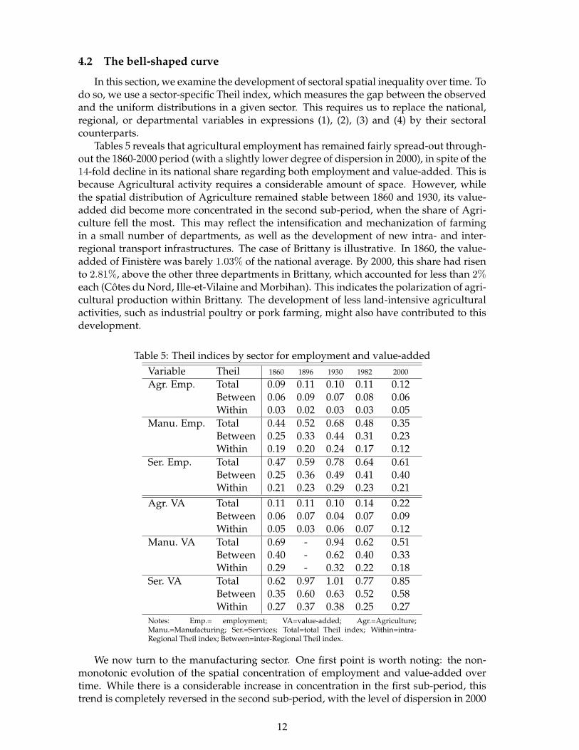
4.2 The bell-shaped curve

In this section, we examine the development of sectoral spatial inequality over time. Todo so, we use a sector-specific Theil index, which measures the gap between the observedand the uniform distributions in a given sector. This requires us to replace the national,regional, or departmental variables in expressions (1), (2), (3) and (4) by their sectoralcounterparts.

Tables 5 reveals that agricultural employment has remained fairly spread-out through-out the 1860-2000 period (with a slightly lower degree of dispersion in 2000), in spite of the14-fold decline in its national share regarding both employment and value-added. This isbecause Agricultural activity requires a considerable amount of space. However, whilethe spatial distribution of Agriculture remained stable between 1860 and 1930, its value-added did become more concentrated in the second sub-period, when the share of Agri-culture fell the most. This may reflect the intensification and mechanization of farmingin a small number of departments, as well as the development of new intra- and inter-regional transport infrastructures. The case of Brittany is illustrative. In 1860, the value-added of Finistere was barely 1.03% of the national average. By 2000, this share had risento 2.81%, above the other three departments in Brittany, which accounted for less than 2%each (Cotes du Nord, Ille-et-Vilaine and Morbihan). This indicates the polarization of agri-cultural production within Brittany. The development of less land-intensive agriculturalactivities, such as industrial poultry or pork farming, might also have contributed to thisdevelopment.

Table 5: Theil indices by sector for employment and value-addedVariable Theil 1860 1896 1930 1982 2000

Agr. Emp. Total 0.09 0.11 0.10 0.11 0.12Between 0.06 0.09 0.07 0.08 0.06Within 0.03 0.02 0.03 0.03 0.05

Manu. Emp. Total 0.44 0.52 0.68 0.48 0.35Between 0.25 0.33 0.44 0.31 0.23Within 0.19 0.20 0.24 0.17 0.12

Ser. Emp. Total 0.47 0.59 0.78 0.64 0.61Between 0.25 0.36 0.49 0.41 0.40Within 0.21 0.23 0.29 0.23 0.21

Agr. VA Total 0.11 0.11 0.10 0.14 0.22Between 0.06 0.07 0.04 0.07 0.09Within 0.05 0.03 0.06 0.07 0.12

Manu. VA Total 0.69 - 0.94 0.62 0.51Between 0.40 - 0.62 0.40 0.33Within 0.29 - 0.32 0.22 0.18

Ser. VA Total 0.62 0.97 1.01 0.77 0.85Between 0.35 0.60 0.63 0.52 0.58Within 0.27 0.37 0.38 0.25 0.27

Notes: Emp.= employment; VA=value-added; Agr.=Agriculture;Manu.=Manufacturing; Ser.=Services; Total=total Theil index; Within=intra-Regional Theil index; Between=inter-Regional Theil index.

We now turn to the manufacturing sector. One first point is worth noting: the non-monotonic evolution of the spatial concentration of employment and value-added overtime. While there is a considerable increase in concentration in the first sub-period, thistrend is completely reversed in the second sub-period, with the level of dispersion in 2000

12

exceeding that in 1860. The Theil indices for 1896, computed in terms of both populationand employment, turn out to be right in between those for 1860 and 1930. Further, all the1982 values fall between those for 1930 and 2000. The spatial concentration of Manufacturingthus follows a bell-shaped curve, as predicted by economic geography. Recall that fallingtransport costs facilitate the concentration of activities with increasing returns. Beyonda certain threshold, transport costs are sufficiently low that differences in market accessbecome secondary to other costs brought about by spatial concentration, so that firmsbegin to relocate to peripheral areas where land is available and cheaper. Figure 2 depictsthe departmental distribution of manufacturing output in 1860, 1930, and 2000, which isunambiguously bell-shaped: in the middle map, the number of dark areas (the top threeclasses) is for instance smaller than in the other two maps (17, compared to 26 and 28).Clearly, very industrialized regions are fewer in 1930 than in 1860 or 2000.14

The same broad trends can be seen in the service sector. The first sub-period is charac-terized by an increase in concentration and the rise of urbanization, which in turn pavedthe way for the development of firm- and consumer-specific services. However, the dis-persion of Services during the second sub-period is less pronounced than for Manufactur-ing. The Theil index for value-added, which is slightly larger in 2000 than in 1982, is theonly exception to the bell-shape; this can be explained by the considerable employmentvolatility in this sector at the end of the century. Overall, we find it fair to say that theseresults are consistent with the bell-shaped curve.

We also want to stress that the bell-shaped curve holds regardless of the spatial scale, Regionsor Departments. However, it is slightly stronger between regions, i.e. the more relevantspatial units for the transport cost-related variables studied by economic geography. Wehave seen in Table 2 that population, employment and value-added have concentratedover the whole period. This suggests that rural-urban migrations in the first sub-periodhave fed the concentration of Manufacturing and Services in cities. By way of contrast,both demographic growth and rural-urban migrations have benefited to second-tier citiesin the second sub-period. This is an important finding as it shows why focusing on thespatial distribution of population and activities as a whole may be misleading.

Because historical data might be more subject to measurement errors, especially be-tween the two World Wars, legitimate concerns may arise about the relevance of 1930 dataand hence, about the robustness of our bell-shaped curve. However, after more than 10years, we can reasonably assume that, in 1930, France has recovered from World War I.Furthermore, the 1931 Census explicitly refers to 1930 data, and the Great Depression onlystarted to impact on industrial production in 1931.15 Nonetheless, we provide robustnesschecks by generating random perturbations in our data set. More precisely, for each de-partment, sector and variable, we draw 1, 000 random values from a normal distributionwith zero-mean and with standard deviations ranging from 0.01 to 0.10. We then computey(1 + e), y being each of our sectoral variables, and e the randomly-generated noise. Last,we compute the mean Theil indices of the so-obtained noisy data series, as well as theirstandard-deviations. Table 6 reports the results for a standard deviation of σ = 0.05, whichmeans that 50% of our randomly-generated variables deviate from the actual data by atmost 5%, 45% by 5 to 10%, and 5% by above 10%.

All numerical values remain consistent with the true values of the Theil indices, whichprovides additional support to the bell-shaped curve.16 The spatial analysis of labor pro-

14It could be argued that the progressive disappearance of Mining and Heavy industries has fostered theconcentration of Manufacturing. However, in France this de-industrialization largely took place after 1960.This makes our point even stronger, as the bell-shaped curve actually declines after 1930.

15Moreover, since our analysis focuses only on differences in the spatial distribution of economic activity,any measurement error that affects all departments equally will have no bearing on our results.

16Tables A.4 and A.5 in the Appendix report the corresponding results for σ = 0.01 and σ = 0.10, respec-

13

Table 6: Theil indices by sector for noisy employment and value-added (σ = 0.05)Variable Theil 1860 1896 1930 1982 2000

Agr. Emp. Total mean 0.10 0.11 0.10 0.11 0.12std. 0.0024 0.0024 0.0025 0.0028 0.0031

Between mean 0.06 0.09 0.07 0.08 0.06std. 0.002 0.0021 0.0023 0.0026 0.0023

Within mean 0.03 0.02 0.03 0.03 0.05std. 0.0014 0.0012 0.0012 0.0014 0.002

Manu. Emp. Total mean 0.44 0.52 0.67 0.48 0.35std. 0.0137 0.0161 0.0199 0.0142 0.0086

Between mean 0.25 0.33 0.44 0.31 0.23std. 0.0089 0.0112 0.0143 0.011 0.0073

Within mean 0.19 0.20 0.24 0.17 0.12std. 0.0058 0.0061 0.0071 0.0048 0.0032

Ser. Emp. Total mean 0.47 0.59 0.78 0.64 0.61std. 0.0177 0.0237 0.0292 0.0221 0.0193

Between mean 0.25 0.36 0.49 0.41 0.40std. 0.0121 0.0165 0.0211 0.0169 0.0155

Within mean 0.21 0.23 0.29 0.23 0.21std. 0.0065 0.0079 0.009 0.0068 0.0058

Agr. VA Total mean 0.11 0.11 0.10 0.14 0.22std. 0.0025 0.0025 0.0025 0.0036 0.0058

Between mean 0.06 0.07 0.04 0.07 0.09std. 0.0022 0.0021 0.0019 0.0022 0.0028

Within mean 0.05 0.04 0.06 0.07 0.12std. 0.0016 0.0014 0.0019 0.0024 0.0039

Manu. VA Total mean 0.70 - 0.94 0.62 0.51std. 0.0226 - 0.0281 0.0174 0.0133

Between mean 0.40 - 0.63 0.40 0.33std. 0.0158 - 0.0206 0.0134 0.0109

Within mean 0.29 - 0.32 0.22 0.18std. 0.0077 - 0.009 0.0059 0.0045

Ser. VA Total mean 0.62 0.97 1.01 0.77 0.85std. 0.0234 0.0347 0.0345 0.026 0.0285

Between mean 0.35 0.60 0.63 0.52 0.58std. 0.0165 0.0254 0.0256 0.0201 0.0224

Within mean 0.27 0.37 0.38 0.25 0.27std. 0.008 0.0102 0.0099 0.0075 0.008

Notes: Emp.= employment; VA=value-added; Agr.=Agriculture; Manu.=Manufacturing; Ser.=Services;Total=total Theil index; Within=intra-Regional Theil index; Between=inter-Regional Theil index; mean:mean value over 1000 replications, std.: standard-deviation over 1000 replications.

14

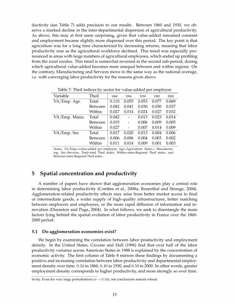
ductivity (see Table 7) adds precision to our results. Between 1860 and 1930, we ob-serve a marked decline in the inter-departmental dispersion of agricultural productivity.As above, this may at first seem surprising, given that value-added remained constantand employment became slightly more dispersed over this period. The key point is thatagriculture was for a long time characterized by decreasing returns, meaning that laborproductivity rose as the agricultural workforce declined. This trend was especially pro-nounced in areas with large numbers of agricultural employees, which ended up profitingfrom the rural exodus. This trend is somewhat reversed in the second sub-period, duringwhich agricultural value-added becomes more unequal between and within regions. Onthe contrary, Manufacturing and Services move in the same way as the national average,i.e. with converging labor productivity for the reasons given above.

Table 7: Theil indices by sector for value-added per employeeVariable Theil 1860 1896 1930 1982 2000

VA/Emp. Agr. Total 0.110 0.055 0.053 0.077 0.069Between 0.082 0.041 0.030 0.050 0.037Within 0.027 0.014 0.024 0.027 0.032

VA/Emp. Manu. Total 0.042 - 0.013 0.023 0.014Between 0.015 - 0.006 0.009 0.005Within 0.027 - 0.007 0.014 0.009

VA/Emp. Ser. Total 0.017 0.020 0.013 0.004 0.006Between 0.006 0.006 0.004 0.003 0.002Within 0.011 0.014 0.009 0.001 0.003

Notes: VA/Emp.=value-added per employee; Agr.=Agriculture; Manu.= Manufactur-ing; Ser.=Services; Total=total Theil index; Within=intra-Regional Theil index; andBetween=inter-Regional Theil index.

5 Spatial concentration and productivity

A number of papers have shown that agglomeration economies play a central rolein determining labor productivity (Combes et al., 2008a; Rosenthal and Strange, 2004).Agglomeration-related productivity effects may arise from better market access to finalor intermediate goods, a wider supply of high-quality infrastructures, better matchingbetween employers and employees, or the more rapid diffusion of information and in-novation (Duranton and Puga, 2004). In what follows, we seek to disentangle the mainfactors lying behind the spatial evolution of labor productivity in France over the 1860-2000 period.

5.1 Do agglomeration economies exist?

We begin by examining the correlation between labor productivity and employmentdensity. In the United States, Ciccone and Hall (1996) find that over half of the laborproductivity variance across American States in 1988 is explained by the concentration ofeconomic activity. The first column of Table 8 mirrors these findings by documenting apositive and increasing correlation between labor productivity and departmental employ-ment density over time: 0.34 in 1860, 0.40 in 1930, and 0.59 in 2000. In other words, greateremployment density corresponds to higher productivity, and more strongly so over time.

tively. Even for very large perturbations (σ = 0.10), our conclusions remain robust.

15

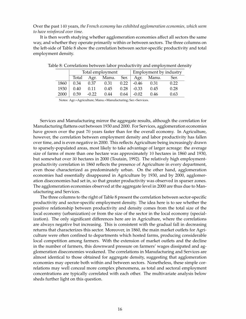
Over the past 140 years, the French economy has exhibited agglomeration economies, which seemto have reinforced over time.

It is then worth studying whether agglomeration economies affect all sectors the sameway, and whether they operate primarily within or between sectors. The three columns onthe left-side of Table 8 show the correlation between sector-specific productivity and totalemployment density.

Table 8: Correlations between labor productivity and employment densityTotal employment Employment by industry

Total Agr. Manu. Ser. Agr. Manu. Ser.1860 0.34 0.37 0.31 0.22 -0.46 0.31 0.221930 0.40 0.11 0.45 0.28 -0.33 0.45 0.282000 0.59 -0.22 0.44 0.64 -0.02 0.46 0.63Notes: Agr.=Agriculture; Manu.=Manufacturing; Ser.=Services.

Services and Manufacturing mirror the aggregate results, although the correlation forManufacturing flattens out between 1930 and 2000. For Services, agglomeration economieshave grown over the past 70 years faster than for the overall economy. In Agriculture,however, the correlation between employment density and labor productivity has fallenover time, and is even negative in 2000. This reflects Agriculture being increasingly drawnto sparsely-populated areas, most likely to take advantage of larger acreage: the averagesize of farms of more than one hectare was approximately 10 hectares in 1860 and 1930,but somewhat over 30 hectares in 2000 (Toutain, 1992). The relatively high employment-productivity correlation in 1860 reflects the presence of Agriculture in every department,even those characterized as predominately urban. On the other hand, agglomerationeconomies had essentially disappeared in Agriculture by 1930, and by 2000, agglomer-ation diseconomies had set in, so that greater productivity was observed in sparser zones.The agglomeration economies observed at the aggregate level in 2000 are thus due to Man-ufacturing and Services.

The three columns to the right of Table 8 present the correlation between sector-specificproductivity and sector-specific employment density. The idea here is to see whether thepositive relationship between productivity and density comes from the total size of thelocal economy (urbanization) or from the size of the sector in the local economy (special-ization). The only significant differences here are in Agriculture, where the correlationsare always negative but increasing. This is consistent with the gradual fall in decreasingreturns that characterizes this sector. Moreover, in 1860, the main market outlets for Agri-culture were often confined to departments which hosted farms, producing considerablelocal competition among farmers. With the extension of market outlets and the declinein the number of farmers, this downward pressure on farmers’ wages dissipated and ag-glomeration diseconomies weakened. The correlations in Manufacturing and Services arealmost identical to those obtained for aggregate density, suggesting that agglomerationeconomies may operate both within and between sectors. Nonetheless, these simple cor-relations may well conceal more complex phenomena, as total and sectoral employmentconcentrations are typically correlated with each other. The multivariate analysis belowsheds further light on this question.

16

5.2 The magnitude of agglomeration economies

Economic geography emphasizes the role of market size and market access in deter-mining both factor prices and the location of economic agents. To evaluate the relativeinfluence of each of these variables, it is customary to regress the logarithm of labor pro-ductivity on the logarithm of employment per unit of surface area (denoted here, densdt fordepartment d at time t), as well as on a number of other explanatory variables. The panelstructure of our data (87 departments, 3 industries, and 3 dates), allows us to introducesector fixed-effects, γs which capture any sector-specific variables that affect all depart-ments in the same way irrespective of time (e.g. labor productivity is on average higherin Manufacturing than in Agriculture), and time fixed-effects, γt, picking up temporalvariations affecting all departments and all sectors equally (e.g. productivity gains fromtechnological progress). Time fixed-effects also correct for the fact that all our variablesare expressed in current francs, and not deflated, which is less arbitrary than choosing aspecific deflator.

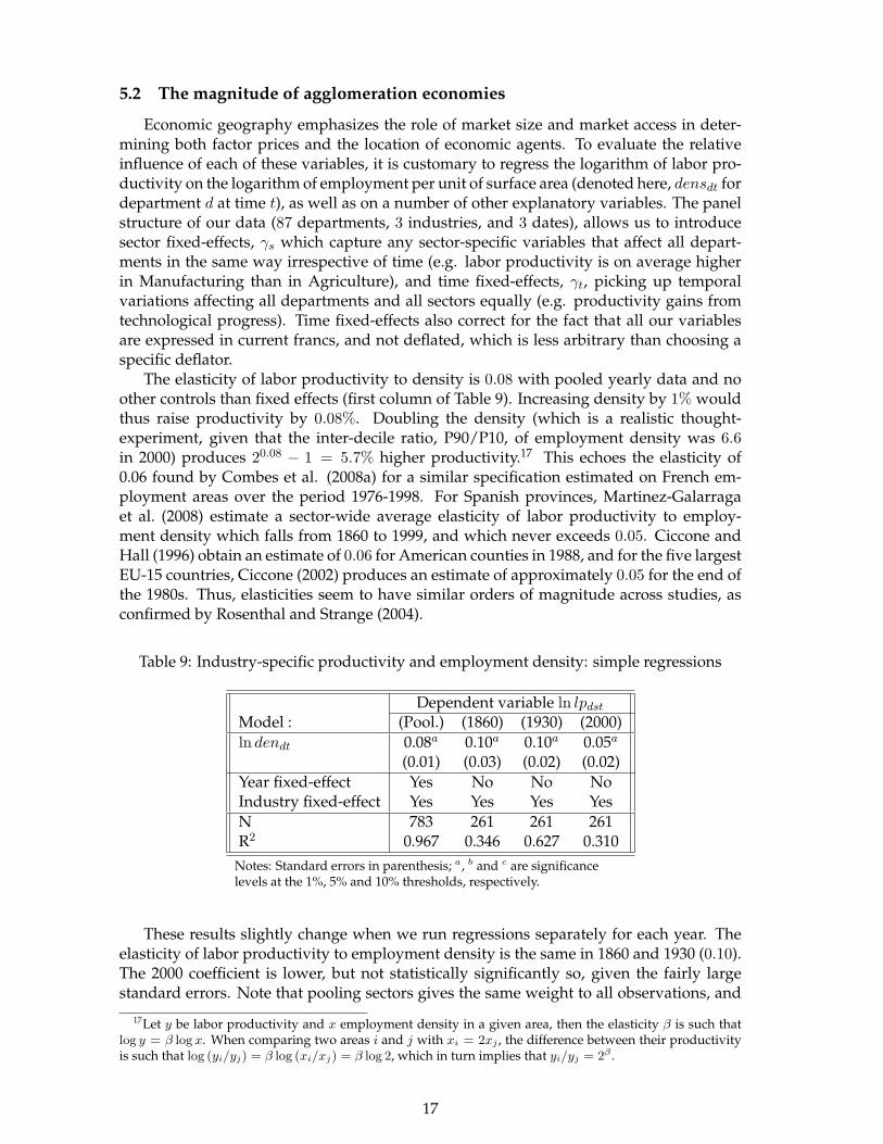
The elasticity of labor productivity to density is 0.08 with pooled yearly data and noother controls than fixed effects (first column of Table 9). Increasing density by 1% wouldthus raise productivity by 0.08%. Doubling the density (which is a realistic thought-experiment, given that the inter-decile ratio, P90/P10, of employment density was 6.6in 2000) produces 20.08 − 1 = 5.7% higher productivity.17 This echoes the elasticity of0.06 found by Combes et al. (2008a) for a similar specification estimated on French em-ployment areas over the period 1976-1998. For Spanish provinces, Martinez-Galarragaet al. (2008) estimate a sector-wide average elasticity of labor productivity to employ-ment density which falls from 1860 to 1999, and which never exceeds 0.05. Ciccone andHall (1996) obtain an estimate of 0.06 for American counties in 1988, and for the five largestEU-15 countries, Ciccone (2002) produces an estimate of approximately 0.05 for the end ofthe 1980s. Thus, elasticities seem to have similar orders of magnitude across studies, asconfirmed by Rosenthal and Strange (2004).

Table 9: Industry-specific productivity and employment density: simple regressions

Dependent variable ln lpdst

Model : (Pool.) (1860) (1930) (2000)ln dendt 0.08a 0.10a 0.10a 0.05a

(0.01) (0.03) (0.02) (0.02)Year fixed-effect Yes No No NoIndustry fixed-effect Yes Yes Yes YesN 783 261 261 261R2 0.967 0.346 0.627 0.310

Notes: Standard errors in parenthesis; a, b and c are significancelevels at the 1%, 5% and 10% thresholds, respectively.

These results slightly change when we run regressions separately for each year. Theelasticity of labor productivity to employment density is the same in 1860 and 1930 (0.10).The 2000 coefficient is lower, but not statistically significantly so, given the fairly largestandard errors. Note that pooling sectors gives the same weight to all observations, and

17Let y be labor productivity and x employment density in a given area, then the elasticity β is such thatlog y = β log x. When comparing two areas i and j with xi = 2xj , the difference between their productivityis such that log (yi/yj) = β log (xi/xj) = β log 2, which in turn implies that yi/yj = 2β .

17

therefore to Agriculture, Manufacturing and Services; in contrast, the data were disaggre-gated in Table 8, thus taking into account the relative importance of different sectors inoverall activity. This may explain the reinforcement of agglomeration economies in theformer case, but not in the latter.

Furthermore, the relatively low R2-values suggest that factors other than density ex-plain productivity differentials across space, and especially so in 1860 and 2000. It is worthstressing that the estimated impact of density may also be tainted by an endogeneity bias.First, employment density may capture the impact of omitted variables, such as special-ization and diversity, access to external outlets, the skill-level of the local labor force, pub-lic facilities, geographical asperities or natural resources. Moreover, employment densityreflects wages, and thus productivity, as workers are drawn to areas with higher wages.The potential bias from this reverse causality comes from the self-reinforcing agglomerationprocess or circular causality discussed in Section 2. As such, we now move to multivariateestimations in order to take more explanatory variables into account, and then to instru-ment some of them.

Endogeneity issue 1: unobserved heterogeneityTo address the endogeneity arising from omitted variables, we add a number of vari-

ables drawn from economic geography. We first control for the departmental surface area,aread. Indeed, density accounts for the market thickness, while land area measures itsspatial extent. For instance, at a given density level, a larger area is likely to have morenon-market interactions among agents than a smaller area because it is more populated.Economic geography also suggests that proximity to large outlets induces greater prof-itability. It is customary to capture this market-access effect with a market potential variablea la Harris (1954). Market potential for department d is defined as the sum of the other de-partments’ (i 6= d) total employment, divided by the interdepartmental distance (distid):18

MPdt =∑i 6=d

empit

distid. (5)

The market potential of an area is defined with respect to all surrounding areas other thanitself, to avoid multicollinearity issues and to identify separately the effects of internaloutlet (i.e. density) and external outlets (i.e. market potential).

We also consider agglomeration economies arising from the sectoral distribution ofeconomic activity. Local specialization is usually measured as the employment share ofsector s in the economic activity of department d at date t, spedst. We estimate the impactof local sectoral diversity via the Herfindhal index, given by the sum of the squares of eachsector’s share in a given department:

Hdt =∑

s(spedst)2.

The lower is Hdt, the greater is the sectoral diversity in department d. To make the esti-mated coefficient easier to interpret, we reformulate the diversity index as divdt = 1/Hdt.

The first column of Table 10 presents the OLS estimates of specification (6):

ln pdst = α+β ln dendt + δ ln aread + η lnMPdt + θ ln spedst +λ ln divdt +γt +γs + εdst, (6)

where pdst is labor productivity in sector s and department d at t, and εdst is an error termthat captures local productivity shocks that are unexplained by the model.

18To compute these interdepartmental distances, we use the latitude and longitude of the departmentalcentroids (provided by the software Mapinfo). We then apply the geodesic (i.e. the shortest route between

18

Table 10: Industry-specific productivity and employment density: multivariate analysisDependent Variables: ln lpdst

Model: (Pool.) (Agr.) (Manu.) (Ser.)ln dendt 0.09a -0.11b 0.13a 0.07a

(0.02) (0.05) (0.02) (0.01)ln aread 0.07c 0.27a 0.04 -0.02

(0.04) (0.08) (0.04) (0.03)lnMPdt 0.16a 0.28a 0.13b 0.01

(0.05) (0.09) (0.05) (0.04)ln spedst -0.05b -0.29a 0.03 0.13a

(0.02) (0.06) (0.06) (0.04)ln divdt 0.61a 1.02a 0.16 0.18b

(0.06) (0.13) (0.14) (0.07)Year fixed-effects Yes Yes Yes YesIndustry fixed-effects Yes No No NoN 783 261 261 261R2 0.972 0.960 0.987 0.992Note: (i) Ordinary Least-Squares. (ii) Standard errors in brackets, robustto departmental clusters in column (Pool.); a, b and c are significancelevels at the 1%, 5% and 10% thresholds, respectively.

The elasticity of density (β = 0.09) is almost not affected by the introduction of theseadditional explanatory variables: at a given surface area, doubling density increases pro-ductivity by 6.4%. Yet, this average value conceals significant disparities between sectors,which is consistent with the correlation analysis presented above. As expected, the effectof density in the agricultural sector (column 2) is negative (β = −0.11), bolstering the ideathat this sector is more productive in sparser regions. However, for Manufacturing andServices (columns 3 and 4), density has a positive and significant impact. A higher elas-ticity is found for Manufacturing (β = 0.13) than for Services (β = 0.07), which may bedue to Manufacturing’s greater reliance on market and supplier access, as well as its needfor skilled labor. In contrast to density, the impact of surface area is not robust: it is onlystatistically significant at the 10% level in the pooled regressions, which may be due to ithaving no effect in Manufacturing and Services (see columns 3 and 4). Surface area doesturn out to play a decisive role in these two sectors once we control for total employmentdensity. This is standard in the literature.

When all sectors are pooled together, the elasticity of market potential is 0.16, whichsuggests that labor productivity is even more responsive to market access than to em-ployment density. However, it should be kept in mind that the larger impact of marketpotential also captures agglomeration economies triggered by labor market pooling andknowledge spillovers diffusing over departmental boundaries. Once again, this averagevalue conceals variation across sectors. The elasticity is highly positive and significantfor Agriculture (η = 0.28), takes on an intermediate value for Manufacturing (η = 0.13),and is essentially zero and insignificant for Services. Proximity to large outlets is impor-tant in Agriculture, probably due to the perishable nature of many products. Access tolarge markets is less important in Manufacturing, which may reflect the sharp decline intransport costs for manufactured goods. Market access plays no role in Services, which isunsurprising since this activity is mostly consumer-oriented and therefore very localizedwithin departments. The coefficients found for density and market potential are thus con-

two points on the Earth’s surface) distance formula.

19

sistent with economic geography priors: agglomeration economies are substantial, landuse varies across sectors because of different congestion effects, and market access mattersa lot.

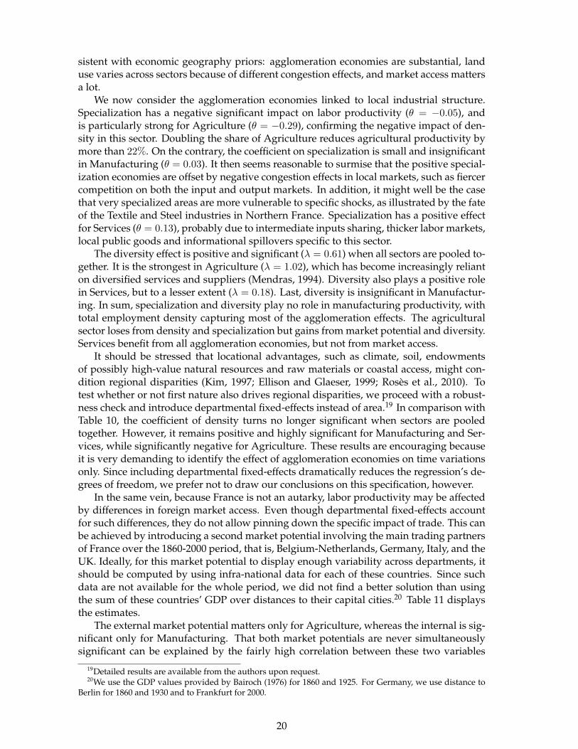
We now consider the agglomeration economies linked to local industrial structure.Specialization has a negative significant impact on labor productivity (θ = −0.05), andis particularly strong for Agriculture (θ = −0.29), confirming the negative impact of den-sity in this sector. Doubling the share of Agriculture reduces agricultural productivity bymore than 22%. On the contrary, the coefficient on specialization is small and insignificantin Manufacturing (θ = 0.03). It then seems reasonable to surmise that the positive special-ization economies are offset by negative congestion effects in local markets, such as fiercercompetition on both the input and output markets. In addition, it might well be the casethat very specialized areas are more vulnerable to specific shocks, as illustrated by the fateof the Textile and Steel industries in Northern France. Specialization has a positive effectfor Services (θ = 0.13), probably due to intermediate inputs sharing, thicker labor markets,local public goods and informational spillovers specific to this sector.

The diversity effect is positive and significant (λ = 0.61) when all sectors are pooled to-gether. It is the strongest in Agriculture (λ = 1.02), which has become increasingly relianton diversified services and suppliers (Mendras, 1994). Diversity also plays a positive rolein Services, but to a lesser extent (λ = 0.18). Last, diversity is insignificant in Manufactur-ing. In sum, specialization and diversity play no role in manufacturing productivity, withtotal employment density capturing most of the agglomeration effects. The agriculturalsector loses from density and specialization but gains from market potential and diversity.Services benefit from all agglomeration economies, but not from market access.

It should be stressed that locational advantages, such as climate, soil, endowmentsof possibly high-value natural resources and raw materials or coastal access, might con-dition regional disparities (Kim, 1997; Ellison and Glaeser, 1999; Roses et al., 2010). Totest whether or not first nature also drives regional disparities, we proceed with a robust-ness check and introduce departmental fixed-effects instead of area.19 In comparison withTable 10, the coefficient of density turns no longer significant when sectors are pooledtogether. However, it remains positive and highly significant for Manufacturing and Ser-vices, while significantly negative for Agriculture. These results are encouraging becauseit is very demanding to identify the effect of agglomeration economies on time variationsonly. Since including departmental fixed-effects dramatically reduces the regression’s de-grees of freedom, we prefer not to draw our conclusions on this specification, however.

In the same vein, because France is not an autarky, labor productivity may be affectedby differences in foreign market access. Even though departmental fixed-effects accountfor such differences, they do not allow pinning down the specific impact of trade. This canbe achieved by introducing a second market potential involving the main trading partnersof France over the 1860-2000 period, that is, Belgium-Netherlands, Germany, Italy, and theUK. Ideally, for this market potential to display enough variability across departments, itshould be computed by using infra-national data for each of these countries. Since suchdata are not available for the whole period, we did not find a better solution than usingthe sum of these countries’ GDP over distances to their capital cities.20 Table 11 displaysthe estimates.

The external market potential matters only for Agriculture, whereas the internal is sig-nificant only for Manufacturing. That both market potentials are never simultaneouslysignificant can be explained by the fairly high correlation between these two variables

19Detailed results are available from the authors upon request.20We use the GDP values provided by Bairoch (1976) for 1860 and 1925. For Germany, we use distance to

Berlin for 1860 and 1930 and to Frankfurt for 2000.

20

Table 11: Industry-specific productivity and employment density: multivariate analysiswith two different market potentials

Dependent Variables: ln lpdst

Model: (Pool.) (Agr.) (Manu.) (Ser.)ln dendt 0.07a -0.11b 0.13a 0.07a

(0.02) (0.05) (0.02) (0.02)ln aread 0.05 0.19b 0.05 -0.01

(0.04) (0.08) (0.05) (0.03)lnMP int

dt 0.08 0.09 0.15b 0.02(0.05) (0.10) (0.06) (0.04)

lnMP extdt 0.15a 0.43a -0.06 -0.01

(0.05) (0.10) (0.06) (0.04)ln spedst -0.05b -0.22a 0.05 0.13a

(0.02) (0.06) (0.07) (0.04)ln divdt 0.53a 0.83a 0.15 0.18b

(0.06) (0.13) (0.14) (0.08)Year fixed-effects Yes Yes Yes YesIndustry fixed-effects Yes No No NoN 783 261 261 261R2 0.973 0.963 0.987 0.992Note: (i) Ordinary Least-Squares. (ii) Standard errors in brackets, robustto departmental clusters in column (Pool.); a, b and c are significancelevels at the 1%, 5% and 10% thresholds, respectively.

(' 0.6) and by the lack of spatial variability of external market potential. Since the coef-ficients of the other variables are almost not affected by introducing the foreign marketpotential, from now on we choose to follow the literature by working with the internalmarket potential only.

Endogeneity issue 2: circular causalityWe follow the procedure proposed by Combes et al. (2008a) to deal with circular causal-

ity. In the first step, we estimate the following equation by ordinary least squares:

ln pdst = ν + θ ln spedst + γdt + γs + εdst, (7)

where γdt is a department-year fixed-effect which captures the influence of local non-sectoral variables on labor productivity. In the second step, we regress the first-step pre-dicted value γdt on density, surface area, market potential, diversity and year fixed-effects,which can be instrumented separately from the first-step estimation:

γdt = α+ β ln dendt + δ ln aread + η lnMPdt + λ ln divdt + γt + ξdt. (8)

Both density and market potential are likely to be endogenous since they depend onworkers’ and firms’ location decisions. Therefore, in the estimation of (8), we instrumentboth variables. A possible estimation strategy would be to plug (8) into (7) and to esti-mate a single specification. This would require to address the endogeneity of all variablessimultaneously. Instead, we proceed in two steps. First, we account separately for two dis-tinct department-sector-time (εdst ) and department-time (ξdt) random terms. This allowsus, in a second step, to tackle the endogeneity of density and market potential without

21

addressing the endogeneity of the other variables, such as specialization.21 Our excludedinstruments are the logs of population density and population potential (i.e. market poten-tial in which population is substituted for employment) in 180122 (denoted dend1801 andMPd1801, respectively), and a peripherality measure (the log of the average distance ofeach department to all the other departments), which is commonly used in the literature.

As shown by the first-stage regressions presented in the Appendix, Table A.6, dueto the strong inertia of the urban hierarchy in France, population densities and marketpotentials at the beginning of the Nineteenth Century are still correlated to employmentdensities and market potentials in 1860, 1930 and 2000. However, it is unlikely that theyare correlated to labor productivity in 1860, 1930 and 2000 because the French economyhas been subjected to a wide range of productivity shocks triggered by wars (from theFrench Revolution to World War II) and rural-urban migrations, which have deeply af-fected the French demography. All of this makes us confident in the economic validity ofour instruments. Yet, there is a need to test their statistical relevance.

Table 12: Industry-specific productivity and employment density: IV estimatesDependent variable γdt

(Pool.) (1860) (1930) (2000)Model : (OLS) (IV) (OLS) (IV) (OLS) (IV) (OLS) (IV)ln dendt 0.09a 0.07a 0.01 0.03 0.09a 0.06b 0.10a 0.09a

(0.02) (0.02) (0.04) (0.04) (0.02) (0.03) (0.02) (0.02)ln aread 0.07c 0.03 -0.05 -0.02 -0.01 -0.05 0.23a 0.21a

(0.04) (0.04) (0.07) (0.07) (0.06) (0.06) (0.05) (0.05)lnMPdt 0.16a 0.16a 0.46a 0.49a 0.08 0.05 0.17a 0.13b

(0.05) (0.06) (0.10) (0.10) (0.06) (0.07) (0.06) (0.06)ln divdt 0.61a 0.60a 0.88a 0.86a 0.63a 0.68a -0.30c -0.29

(0.06) (0.06) (0.08) (0.07) (0.11) (0.11) (0.17) (0.19)Year fixed-effects Yes Yes No No No No No NoN 261 261 87 87 87 87 87 87R2 0.991 - 0.678 - 0.458 - 0.442 -Cragg-Donald F-Stat - 148.3 - 155.3 - 65.0 - 43.2Hansen J-Stat - 1.963 - 0.616 - 0.415 - 4.012Chi-sq(1) P-value - 0.16 - 0.43 - 0.52 - 0.05Endogeneity C-Stat - 4.622 - 5.567 - 7.530 - 2.095Chi-sq(2) P-value - 0.10 - 0.06 - 0.02 - 0.35Shea’s partial R2 (ln dendt) - 0.645 - 0.852 - 0.709 - 0.616Shea’s partial R2 (lnMPdt) - 0.879 - 0.970 - 0.915 - 0.853Notes: (i) IV Generalized Method of Moments; Density and market potential instrumented: excluded in-struments are the logs of population density and market potential in 1801, and the log of average distanceto all other departments; First-stage regressions are reported in the Appendix, Table A.6. (ii) Standard errorsin brackets, robust to departmental clusters in column (Pool.); a, b and c are significance levels at the 1%, 5%and 10% thresholds, respectively. (iii) Stock and Yogo (2005) critical values for the Cragg- Donald F-Statisticare 13.97 for a 5% maximum IV bias and 8.78 for a 10% maximal IV bias.

To this end, Table 12, which reports the results of IV regressions, also displays the fol-lowing statistics. (i) The Shea’s partial R2 shows that our instruments explain quite a largeshare of the instrumented variables, once potential inter-correlations among instrumentshave been accounted for. However, we have to check that this is not done at the expense

21More details are provided in Combes et al. (2008a and 2010).22Since departments were created in 1790, population data are not available at this jurisdiction level before

1801, which is the year of the first French Census.

22

of their strength. To this end, we compute (ii) the Cragg-Donald F-Statistic, which checkswhether the excluded instruments are only weakly-correlated with the endogenous re-gressors. Instruments are not weak if the statistic is above the critical values provided byStock and Yogo (2005). This holds here because the critical values, which depend both onthe numbers of instrumented variables and of instruments, are 13.97 for a 5% maximum IVbias and 8.78 for a 10% maximal IV bias. (iii) The Hansen J-Statistic tests over-identifyingrestrictions. Instruments are exogenous when their p-value are higher than 5%. This holdsfor all regressions. All together, these tests support the validity of our instruments. Finally,(iv) the C-Statistic tests whether instrumented regressors are endogenous. If the p-valueis large, they are endogenous, and instrumentation is needed. This is likely to arise forpooled regressions, for 2000 and, to a lower extent, for 1860, but not for 1930, for whichOLS should be preferred.

Endogeneity leads to an overestimation of the density premium by approximately 20%.This is in line with Combes et al. (2008a and 2010) who focus on the 1976-1998 period.Moreover, the coefficients on market potential and the other variables are only little af-fected by instrumentation. Our findings are, therefore, robust to reverse causality andmissing variables issues that could affect both density and market potential.

5.3 The role of human capital

New growth theories emphasize the role of human capital as a determinant of produc-tivity (Lucas, 1988). In this context, the positive effect of density may stem from denserareas (in particular cities) having a greater share of skilled labor (Combes et al., 2008a).This can be tested by adding variables capturing the skills of the local labor force. Thelinear approximation to a Cobb-Douglas production function requires adding the share ofskilled labor as an explanatory variable (Hellerstein et al., 1999). We thus estimate now:

γdt = α+ β ln dendt + δ ln aread + η lnMPdt + λ ln divdt + µHCdt + γt + ξdt,

whereHCdt is a proxy for the share of skilled workers in department d at date t. The coeffi-cient µ is of a different nature to the other regression coefficients since it is not an elasticity.We test whether the introduction of human capital impacts positively labor productivityand whether it leaves the other estimated coefficients unchanged.

Given the time span, there is no chance of constructing a meaningful and homogenoushuman-capital measure. Average education has grown considerably over time, especiallysince World War II. Given the small number of students who obtained the baccalaureatein 1860 and 1930, it seems reasonable to choose (for the first sub-period) enrollment inelementary schools as a proxy for human capital. The only available departmental-leveldata are for 1863 and 1933 (Daures et al., 2007; Rivet, 1936). The average departmentalratio of the number of pupils to the labor force was 25% in 1863 and only 27% in 1933.This lack of movement in schooling over a long period likely makes the 1863 and 1933figures good approximations to the unobserved 1860 and 1930 values. Admittedly, pri-mary school enrollment is a very rough measure of human capital as we expect skills andknowledge to be embodied in various types of craftsmanship. However, measuring theselearning-by-doing effects is extremely difficult.

As detailed Census data are available for 1999, we use them to build a more precisemeasure of departmental human capital in 2000. Averaging across all departments, theshare of employees whose reported educational attainment is elementary school is 12.2%,with figures of 45.1% for middle school, 18.4% for high school, and 24.3% for graduate andpost-graduate. Since these shares add up to 1, we drop one category from the regression,high school, HCdt(3), retaining elementary school, HCdt(1) in order to allow for inter-

23

period comparisons, middle school, HCdt(2), and graduate studies, HCdt(4), which mayaffect labor productivity through either professional specialization or human capital.

To address the heterogeneity of these measures across time, we split the sample intotwo subsets. Moreover, we drop the surface area, which was insignificant in most previousestimations, in order to use it as an instrument for our human capital variable, and increasethe chance to succeed in a demanding instrumentation task.23

Table 13: The effect of human capital 1860-1930Dependent variable: γdt

(OLS1) (OLS2) (IV1) (IV2)ln dendt 0.07a 0.08a 0.07a 0.06a

(0.02) (0.02) (0.03) (0.02)lnMPdt 0.22a 0.21a 0.24a 0.27a

(0.06) (0.05) (0.06) (0.06)ln divdt 0.74a 0.68a 0.69a 0.67a

(0.06) (0.07) (0.06) (0.07)HCdt 0.41b 0.37b 0.45c

(0.18) (0.18) (0.27)Year fixed-effect Yes Yes Yes YesN 174 174 174 168R2 0.987 0.987 - -Cragg-Donald F-Stat - - 253.5 10.6Hansen J-Stat - - 0.023 9.129Chi-sq P-value - - 0.88 0.10Endogeneity C-Stat - - 4.00 5.7Chi-sq P-value - - 0.14 0.13Shea’s partial R2 (ln dendt) - - 0.821 0.824Shea’s partial R2 (lnMPdt) - - 0.894 0.902Shea’s partial R2 (HCdt) - - - 0.354Notes: (i) IV Generalized Method of Moments. Density and market potentialinstrumented in column (IV1): excluded instruments are the logs of populationdensity and potential in 1801, and the average distance to all other departments;Density, market potential and human capital instrumented in column (IV2): ex-cluded instruments are the logs of population density in 1801, 1806 and 1836,the logs of population potential in 1806 and 1836, the log of the average dis-tance to all other departments, the log of the surface area, and the departmentalratio of the number of pupils in 1837 to population in 1836; first-stage regres-sions are reported in the Appendix, Table A.7. (ii) Human capital is missing forthree departments in 1837 (Alpes-Maritimes, Savoie and Haute-Savoie), whichlowers the number of observations in (IV2). (iii) Standard errors in brackets,robust to departmental clusters in column (Pool.); a, b and c are significancelevels at the 1%, 5% and 10% thresholds, respectively. (iv) For (IV1), the Stockand Yogo (2005) critical values for the Cragg-Donald F-Statistic are 13.97 for a5% maximum IV bias, and 8.78 for a 10% maximal IV bias. For (IV2), the Stockand Yogo (2005) critical values for the Cragg-Donald F-Statistic are 16.80 for a5% maximum IV bias, and 9.64 for a 10% maximal IV bias.

Table 13 report our estimates for the 1860-1930 period. As a benchmark, columns(OLS1) and (OLS2) report the OLS coefficients drawn from estimating equation (6) withand without human capital. Columns (IV1) and (IV2) report the two IV-counterparts ofcolumn (OLS2). Specifically, in column (IV1), variables ln dendt and lnMPdt are instru-

23The results of first-stage regressions are provided in the Appendix, Table A.7.

24

mented by population density and market potential in 1801, as well as by the average dis-tance to all other departments. In column (IV2), we go one step further than the literatureby instrumenting human capital, which may be endogenous. Indeed, skilled workers aremore likely to move to the most productive areas than the unskilled, because these areasoffer higher wages and consumption amenities they value. If such unobserved amenitiesare correlated with productivity gains, human capital has to be instrumented. With infor-mation on primary schools dating back to 1837, we use as instruments the departmentalratio of the number of pupils in 1837 to population in 1836, population densities in 1801,1806 and 1836, and population potentials in 1806 and 1836, as well as the surface area. For2000, we consider as instruments the departmental ratio of the number of pupils in 1837to population in 1836, the departmental ratios of the number of pupils to the labor force in1860 and 1930, population density and potential in 1801, employment density and marketpotential in 1860, as well as the surface area.

Human capital has a positive and significant effect on labor productivity, even thoughit does not increase the R2, which was already very high. Although estimates are plaguedby a slight endogeneity bias, this positive impact is robust to instrumentation, even ifprecision is lost. The Cragg-Donald F-Statistic, the Hansen J-Sstatistic and the endogeneityC-Statistic speak in favor of the instruments validity and the need to instrument. Theinclusion of human capital does not affect the elasticities of density, market potential anddiversity. This is likely due to the relatively uniform spatial distribution of the share ofelementary education (the corresponding coefficients of variation are 0.33 and 0.16 for 1860and 1930, respectively) and, more importantly, to the weak negative correlation betweenemployment density (in log) and human capital (−0.31 in 1860, −0.23 in 1930). This isconsistent with the observed small rise in the elasticity of productivity to density whenhuman capital is added as an explanatory variable.

All these figures support the conclusion that agglomeration economies are not gener-ated by human capital over the 1860-1930 period. Rather, education fostered developmentin all areas, especially those which were less densely populated where it was better. Thismay be surprising since the Jules Ferry laws, which made elementary schooling manda-tory over all of France, were enacted only in 1881-1882. However, recent econometric workby Diebolt et al. (2005) reveals that educational convergence across French departmentsbegan as early as the time of the July Monarchy and the Second Empire. By imposing afixed minimum wage for teachers, the Guizot law of the 29th of June 1833 made a startto the leveling of educational costs across French local jurisdictions. The Law of April 10,1867, which ordained the development of Girls’ schools and introduced free education inall jurisdictions which wanted it, reinforced this convergence. Overall, while human capitalpositively affects labor productivity over the 1860-1930 period, it is not conducive to agglomerationeconomies.

Table 14 reproduces the analysis in Table 13, but for 2000. In the benchmark OLS esti-mations, it is worth underlining that human capital variables are very significant and raisethe R2 significantly, contrary to the 1860-1930 estimation. In addition, density and marketpotential become insignificant once human capital is controlled for. The decrease in thedensity premium is in line with the literature. For example, Combes et al. (2008a) showthat, after controlling for abilities and skills, the density elasticity of French wages fallsfrom 0.063 to 0.030. Here, the density premium is totally washed out by human capital. Itshould be kept in mind that this extreme result is drawn from aggregated data, whereasCombes et al. (2008a) consider an individual fixed-effect controlling for unobserved abili-ties. As for market potential, it may not matter anymore because France has experienceda substantial fall in transport costs over the last few decades (Combes and Lafourcade,2005), which has made the market potential almost the same across departments.

25

Table 14: The effect of human capital 2000Dependent variable: γdt

(OLS1) (OLS2) (IV1) (IV2)ln dendt 0.06c 0.02 0.02 -0.06

(0.02) (0.04) (0.04) (0.06)lnMPdt 0.17a 0.11 0.02 0.11

(0.06) (0.08) (0.09) (0.08)ln divdt -0.27 -0.75a -0.74a -1.51a

(0.18) (0.25) (0.26) (0.47)HCdt(1) 2.71b 3.74a 4.63b

(1.207) (1.42) (2.22)HCdt(2) 4.04a 3.98a 13.28a

(1.56) (1.43) (2.43)HCdt(4) 3.61b 4.09b 10.95a

(1.52) (1.69) (3.35)N 87 87 87 84R2 0.306 0.399 - -Cragg-Donald F-Stat - - 42.49 1.38Hansen J-Stat - - 4.148 4.110Chi-sq P-value - - 0.04 0.39Endogeneity C-Stat - - 5.34 21.74Chi-sq P-value - - 0.07 0.00Shea’s partial R2 (ln dendt) - - 0.621 0.354Shea’s partial R2 (lnMPdt) - - 0.838 0.502Shea’s partial R2 (HCdt(1)) - - - 0.325Shea’s partial R2 (HCdt(2)) - - - 0.250Shea’s partial R2 (HCdt(4)) - - - 0.238Notes: (i) IV Generalized Method of Moments; Density and market potentialinstrumented in column (IV1): excluded instruments are the logs of populationdensity and potential in 1801, and the average distance to all other departments;Density, market potential and human capital variables instrumented in column(IV2): excluded instruments are the logs of population density and potential in1801, the logs of employment density and market potential in 1860, the log ofaverage distance to all other departments, the log of the surface area, the de-partmental ratio of the number of pupils in 1837 to population in 1836, and thedepartmental ratios of the number of pupils to the labor force in 1860 and 1930;First-stage regressions are reported in the Appendix, Table A.8. (ii) Humancapital is missing for three departments in 1837 (Alpes-Maritimes, Savoie andHaute-Savoie), which lowers the number of observations in (IV2). (iii) Standarderrors in brackets, robust to departmental clusters in column (Pool.); a, b and c

are significance levels at the 1%, 5% and 10% thresholds, respectively. (iv) For(IV1), the Stock and Yogo (2005) critical values for the Cragg-Donald F-Statisticare 18.76 for a 5% maximum IV bias, and 10.58 for a 10% maximal IV bias.For (IV2), the Stock and Yogo (2005) critical values do not exist, the number ofinstrumented variables being too large.

26

To shed further light on this, a discussion on the impact of each type of human capital iswarranted. As previously, elementary schooling remains negatively correlated with den-sity (−0.37) and homogeneously distributed across departments (the coefficient of vari-ation of the share of elementary education is 0.20). Similarly, since middle schooling isalso negatively correlated with density (−0.61), we expect both variables to have a deeperpositive impact on labor productivity in less-populated areas. This is consistent with thedeclining part of the bell-shaped curve: an increasing number of industrial plants, whichemploy a large share of low-educated workers, move away from large urban centers toless urbanized areas where they find the types of workers they need. By way of contrast,to the extent that the correlation between density and the share of graduate students inemployment is large and positive (0.74), it is reasonable to conclude that, in 2000, highereducation is the main driver of agglomeration economies. This sharply contrasts withthe period 1860-1930 and suggests that today migrants are high-skilled workers, whereasmost of the Nineteenth Century migrants, freed from farming, were low-skilled.

As shown by the last two columns of Table 14, the instrumentation confirms the abovefindings. If anything, all human capital variables matter even more after instrumentationas their coefficients are much larger than in column (OLS2). Hence, unlike what we ob-serve for the 1860-1930 period, these results provide strong evidence that the impact ofdensity is overestimated when human capital is not controlled for.24 To sum up, over therecent period, higher education has superseded both density and market potential in thedetermination of the spatial distribution of labor productivity.25

6 Conclusion

Our cliometric analysis has uncovered evidence consistent with two fundamental pre-dictions of economic geography. Firstly, the spatial distribution of Manufacturing andServices has traced out a bell-shaped curve since the mid-Nineteenth Century: an increasein spatial concentration in the 1860-1930 period was followed by increasing dispersionover 1930-2000. The explanation we suggest for this phenomenon is the sustained declinein transport costs.

Secondly, the main force behind this bell-curve is the existence of agglomeration economiesin Manufacturing and Services. Over 1860-1930, the benefits reaped by spatial proximityare triggered mainly by the density of economic activity, market access and diversity. Byway of contrast, higher education is by far the main agglomeration force in 2000. As ex-pected, only Agriculture is more efficient in more sparsely-populated regions. We alsoshow that total employment and value-added have become heavily concentrated overthe whole 1860-2000 period. This suggests that rural-urban migrations in the sub-period1860-1930 have fed the concentration of Manufacturing and Services in cities. By way

24Despite the very similar results drawn from columns (OLS2), (IV1) and (IV2) in Table 14, it is hard to assesswhich specification should be preferred from the econometric point of view. However, we have to keep inmind that instrumenting our three human capital variables, together with density and market potential is verydemanding. In column (IV2), the instruments are exogenous according to the Hansen’s tests. However, theCragg-Donald F-Statistic is pretty low, which suggests that instruments could be weak, even though criticalvalues are not available to properly test this. Furthermore, the C-test concludes that instrumented variablesare not endogenous and, therefore, should not be instrumented. Yet, when human capital is not instrumented,the C-test confirms that density and market potential are endogenous and thus, need to be instrumented. Eventhough our instruments are strong in this case, they are not very exogenous. Anyway, we are confident in ourresults because all specifications lead to similar parameter estimates.

25Regarding diversity, the negative coefficient could be somewhat surprising. However, it is not reallya matter of concern because recent empirical contributions have shown that its effect does depend on theselected control variables and instruments used.

27

of contrast, both demographic growth and rural-urban migrations have also benefited tosecond-tier cities in the sub-period 1930-2000.

Contrary to general belief, however, we have shown that labor productivity has be-come more equally distributed across French space. Spatial concentration being more pro-nounced in increasing-return-to-scale-industries, migrations along both the spatial andsectoral dimensions have favored an equalization of wages across space. Conversely, thelaw of diminishing returns has made the labor-depleted agricultural regions more produc-tive, which has triggered a “catch-up” of rural areas.

References

Bairoch, P. 1997. Victoires et deboires. Histoire economique du monde du XVIe sieclea nos jours. Paris: Gallimard.

Barrios, S., Strobl, E., 2009. The dynamics of regional inequalities. Regional Scienceand Urban Economics 39, 575-591.

Caron, F., 1997. Histoire des chemins de fer en France : 1740 - 1883. Paris: Fayard.Ciccone, A., 2002. Agglomeration Effects in Europe. European Economic Review 46

(2), 213-227.Ciccone, A., Hall, R.E., 1996. Productivity and the density of economic activity. Amer-

ican Economic Review 86 (1), 54-70.Combes, P.-P., Duranton, G., Gobillon, L., 2008a. Spatial wage disparities: sorting mat-

ters! Journal of Urban Economics 63 (2), 723-742.Combes, P.-P., Duranton, G., Gobillon, L., Roux, S., 2010. Estimating agglomeration

economies with history, geology, and worker effects. In Glaeser, E L. (Ed.) AgglomerationEconomics. Cambridge, MA: NBER pp. 15-65.

Combes, P.-P., Lafourcade, M., 2005. Transport costs: measures, determinants, andregional policy implications for France. Journal of Economic Geography 5 (3), 319-349.

Combes, P.-P., Mayer, T., Thisse, J.-F., 2008b. Economic geography. The integration ofregions and nations. Princeton, NJ: Princeton University Press.

Daures, N., Diebolt C., Jaoul-Grammare, M., San Martino G., 2007. L’instruction pri-maire en France au 19eme siecle. Une etude cliometrique du mythe de Ferry. Economieset Societes, Serie AF 41 (7-8), 1089-1363.

Delefortrie, N., Morice, J., 1959. Les revenus departementaux en 1864 et 1954. Paris:Armand Colin.

Desaigues, B., forthcoming. La reconstitution du produit industriel regional francaispour la periode 1860-1866. Economies et Societes.

Diebolt, C., Jaoul, M., San Martino, G., 2005. Le Mythe de Ferry : une analyse cliometrique.Revue d’Economie Politique 115 (5), 471-497.

Duranton, G., Puga, D., 2004. Micro-foundations of urban increasing returns: theory.In: Henderson, V., Thisse, J.-F. (Eds.), Handbook of Regional and Urban Economics, vol.4. Elsevier, Amsterdam, pp. 2063-2117.

Eaton, J., Eckstein, Z., 1997. Cities and growth: theory and evidence from France andJapan. Regional Science and Urban Economics 27 (4-5), 443-474.

Ellison, G., and E.L. Glaeser, 1999. The geographic Concentration of Industry: DoesNatural Advantage Explain Agglomeration?. American Economic Review 89 (2), 311-316.

Fontvieille, L., 1976. Evolution et croissance de l’Etat francais 1815-1969. Economie etSocietes, Serie AF 13, 1833-1835.

Fontvieille, L., 1982. Evolution et croissance de l’Administration departementale francaise,1815-1974. Economies et Societes, Serie AF 14, 149-173.

28

Fujita, M., Krugman, P., Venables, A.J., 1999. The Spatial Economy. Cities, Regions andInternational Trade. Cambridge MA: The MIT Press.

Glaeser, E.L., Kallal, H.D., Scheinkman, J.A., Shleifer, A., 1992. Growth in cities. Jour-nal of Political Economy 100 (6), 1126-1152.

Glaeser, E.L., Kohlhase, J.E., 2004. Cities, regions and the decline of transport costs.Papers in Regional Science 83, 197–228.

Harris, C.D., 1954. The market as a factor in the localization of industry in the UnitedStates. Annals of the Association of American Geographers 64 (4), 315-348.

Head, K., Mayer, T., 2004. Market potential and the location of Japanese investment inthe European Union. Review of Economics and Statistics 86, 959-972.

Hellerstein, J.K., Neumark, D., Troske, K.R., 1999. Wages, productivity, and workercharacteristics: evidence from plant-level production functions and wage equations. Jour-nal of Labor Economics 17 (3), 409-446.

Henderson, V., Kuncoro, A., Turner, M., 1995. Industrial development in cities. Journalof Political Economy 103 (5), 1066-1090.

Institut de Conjoncture, 1944. Le produit technique en France depuis 100 ans, Etudespeciale no3. Paris: Imprimerie Nationale.

INSEE, 1957. Les comptes economiques de l’annee 1938. Paris.INSEE, 1966. Annuaire Statistique de la France. Paris.Kim, S., 1995. Expansion of markets and the geographic distribution of economic ac-

tivities: the trends in U.S. regional manufacturing structure, 1860-1987. Quarterly Journalof Economics 110 (4), 881-908.

Kim, S., 1998. Economic integration and convergence: U.S. regions, 1840-1987. Journalof Economic History 58 (3), 659-683.

Kim, S., Margo, R.A., 2004. Historical perspectives on U.S. economic geography. In:Henderson, V., Thisse, J.-F. (Eds.), Handbook of Regional and Urban Economics, vol. 4.Elsevier, Amsterdam, pp. 2981-3020.

Leveque, P., 1980. La patente, indicateur de croissance economique differentielle auXIXeme siecle. Bulletin 13 de l’Association Francaise des Historiens Economistes.

L’Hardy, P., 1976. Une representation geometrique de la procedure R.A.S. dans le casle plus simple. Annales de l’INSEE (22-23), 283-291.

Lucas, R.E., 1988. On the mechanics of economic development. Journal of MonetaryEconomics 22, 3-22.

Marchand, O., Thelot, C., 1991. Deux siecles de travail en France. Paris: INSEE, Col-lection Etudes.

Martinez-Galarraga, J., Paluzie, E., Pons, J., Tirado, D., 2008. Agglomeration andlabour productivity in Spain over the long term. Cliometrica 2 (3), 195-212.

Mendras, H., 1994. La Seconde Revolution francaise 1965-1984. Paris: Gallimard.Merlin, P., 2010. L’amenagement du territoire en France. La Documentation francaise,

Paris.Moretti, E., 2004. Human capital externalities in cities. In: Henderson, V., Thisse, J.-F.

(Eds.), Handbook of Regional and Urban Economics, vol. 4. Elsevier, Amsterdam, pp.2243-2291.

Morrisson, C., 2000. Historical perspectives on income distribution: the case of Eu-rope. In: Atkinson, A.B., Bourguignon, F. (Eds.), Handbook of Income Distribution, vol. 1.Elsevier, Amsterdam, pp. 217-260.

Paluzie, E., Pons, J., Tirado, D.A., 2004. The geographical concentration of industryacross Spanish regions. 1856-1995. Review of Regional Research 24 (2), 143-160.

Piketty, T., Postel-Vinay, G., Rosenthal, J.-L., 2006. Wealth concentration in a develop-ing economy: Paris and France, 1807-1994. American Economic Review, 236-256.

29

Redding, S., Sturm, D., 2008. The cost of remoteness: evidence from German divisionand reunification. American Economic Review 98 (5), 1766-1797.

Redding, S., Venables, A.J., 2004. Economic geography and international inequality.Journal of International Economics 62, 53-82.

Rivet, R., 1936. L’enseignement primaire en France depuis la guerre. Bulletin de laStatistique generale de la France et du Service d’observation des Prix. Tome XXV, FasciculeII, 291-333.

Rosenthal, S.S., Strange, W.C., 2004. Evidence of the nature and sources of agglomer-ation economies. In: Henderson, V., Thisse, J.-F. (Eds.), Handbook of Regional and UrbanEconomics, vol. 4. Elsevier, Amsterdam, pp. 2119-2171.

Roses, J.R., 2003. Why isn’t the whole of Spain industrialized? New economic geogra-phy and early industrialization, 1797-1910. Journal of Economic History 63 (4), 995-1022.

Roses, J.R., Martinez-Galarraga, J., Tirado, D.A. 2010. The upswing of regional incomeinequality in Spain (1860-1930). Exploration of Economic History 47, 244-257.

Singer-Kerel, J., 1961. Le cout de la vie a Paris de 1840 a 1954. Paris: Armand Colin.Statistique Generale de la France, 1891 and 1931. Annuaire Statistique. Paris: Im-

primerie Nationale.Stock, James H. and Motohiro Yogo, 2005. Testing for Weak Instruments in IV Regres-

sion in Identification and Inference for Econometric Models: A Festschrift in Honor of ThomasRothenberg, Donald W. K. Andrews and James H. Stock, eds. Cambridge University Press,pp.80-108.

Theil, H., 1967. Economics and Information Theory. Amsterdam: North-Holland.Tirado, D.A., Paluzie, E., Pons, J. 2002. Economic integration and industrial location:

the case of Spain before World War I. Journal of Economic Geography 2, 343-363.Toutain, J.-C., 1963. La population de la France de 1700 a 1959. Cahiers de l’ISEA, Serie

AF 3 (supplement 133), 1-253.Toutain, J.-C., 1967. Les transports en France de 1830 a 1965. Economie et Societes,

Serie AF 9 (8), 7-306.Toutain, J.-C., 1987. Le produit interieur brut de la France de 1789 a 1982. Economies

et Societes Serie AF 15 (5), 49-237.Toutain, J.-C., 1992. La production agricole de la France de 1810 a 1990 : departements

et regions. Economies et Societes Serie AF 17 (11-12 and 1-2-3-4)Toutain, J.-C., 1997a. La croissance francaise, 1789-1990, nouvelles estimations. Economie

et Societes Serie HEQ 1 (1), 5-136.Toutain, J.-C., 1997b. L’imbroglio des indices de prix francais du XIXe siecle. Economies

et Societes, Serie HEQ 1 (1), 137-187.Vincent, A., 1962. Evolution de la production interieure brute en France de 1896 a 1938.

Etudes et conjoncture 11, p.931.Williamson, J., 1965. Regional Inequality and the Process of National Development: A

Description of the Patterns. Economic Development and Cultural Change 13 (1), 3-45.Wolf, N. 2007. Endowments vs. market potential: What explains the relocation of

industry after the Polish reunification in 1918? Exploration in Economic History 44, 22-42.

Appendix

The Data

Agricultural outputDomestic agricultural product is calculated from the Agriculture Surveys of 1862, 1892

and 1929. Regarding the Agricultural Survey of 1862, data collection took place that same

30

year, but a number of 1865 prices were used and the survey was published in 1868-1870.The survey is fairly exhaustive and allows us to distinguish between seeds, animal con-sumption, food-industry consumption, and human consumption. The values obtained foreach category closely match those in Delefortrie and Morice (1959). As for the AgriculturalSurvey of 1929, it was ordained by the 27th December 1927 Finance Law; while the brunt ofthis survey was conducted in 1929, it was meticulously inspected for errors and correctedfrom 1930 to 1933, and was only published in 1939. The 1892 survey is also very detailed,but required a certain number of corrections, as discussed in Toutain (1992).

Manufacturing outputDesaigues (forthcoming) has meticulously reconstructed data for Manufacturing value-

added by department. The two sources she uses are: (i) the Survey of 1860 conducted bythe Parisian Chamber of “Commerce” in 1860, that was published in 1864 (for Paris); and(ii) the Manufacturing Survey labeled as 1862, but which actually covers the 1861-1865period, that was published in 1873 (for the rest of France). This last survey is drawn froma poll conducted at the Arrondissement-level for a total of 16 sectors (including State-owned industries). The industry-level value-added data from this poll are then appliedto the whole manufacturing labor force. While this survey defines Manufacturing in themodern sense, it does not include craftsmanship. Desaigues overcomes this shortcomingby imputing the value-added of a representative sample of polled firms with fewer thanfive workers to craftsmanship. Total value-added is then obtained by adding these twoManufacturing figures to the 1860 Parisian data.

Toutain uses the Manufacturing Survey provided in the Census Appendix of 1931 forthe 1930 data. Only one quarter of the 60,000 questionnaires sent to existing firms with atleast 10 workers (62, 546 enterprises) were filled in appropriately. Hence, not all sectorswere surveyed and some activities were covered only partially.26 Despite these seriouspitfalls, information can be extrapolated to the whole population of industrial workers,including firms with fewer than 10 workers. In fact, 75% of the latter belong to the highly-skilled craftsmanship sector, e.g. pork butchers, millers, pastry cooks, cabinet makers andfurriers. Absent data regarding these workers, Toutain assumes that their value-addedwas no less than that of workers in large firms. This approximation is admittedly hardto check, but does not seem unrealistic, as craftsmen’s output attracted relatively highprices.27

Service outputService output data for 1860, 1896 and 1930 are drawn from the 1861, 1896 and 1931

Censuses. They are obtained as the sum of two components. First, Toutain (1967) adds upthe value-added of all Transportation sub-industries (roads, railroads, sea-transport underthe French flag, coastal navigation, navigable rivers and air-transport) to create a nationalaggregate. This latter is then assigned across departments according to the size of the localTransportation labor force.28 Second, Toutain (1963, 1987, 1997a) adds up the revenuesstemming from five Service groups: Housing, Public Services, Retailing and Wholesale,Professions, and Household Services.

(i) Housing rents for 1860 and 1896 are drawn from the net incomes reported in theFiscal Surveys of 1851-1853 and 1887-1889 respectively (Statistique Generale de la France,1891). A linear interpolation was applied to fill in the 1860-1865 period. For 1930, the totalvalue of housing rents was estimated by Duge de Bernonville (Institut de Conjoncture,

26For example, more than 40% of the Metal industry was covered, but only 16% of the Textile industry.27In 1957, the INSEE published “Les comptes economiques de l’annee 1938” (INSEE, 1957). This document

provides 1938 value-added for 7 industrial sectors. The sectoral shares are very similar to those obtained byToutain.

28Sea transport represents only a small share (less than 5%) of the total value-added in TransportationServices, so its allocation to landlocked Departments does not produce major distortions.

31

1944, p.109). Departmental rents are provided by the Statistique Generale de la France(1931) and are prorated so as to match the national value obtained by Duge de Bernonville.

(ii) Public-sector wages were reconstructed by Fontvieille (1976, 1982) using State andlocal community yearly account records. The sum of these wages is then prorated acrossdepartments, based on the size of the local public-sector labor force.

(iii) The retail and wholesale incomes of licensed and non-licensed workers are con-structed as follows. In 1860, according to the French Fiscal Administration, the profes-sional tax (“patentes” in French)29 accounted for 3% of licensed-workers’ incomes. In 1896and 1930, the total income of licensed workers is obtained from Vincent (1962, p.931).These two figures are prorated across departments, based on professional tax (1930). Asfor non-licensed workers, departmental wages are computed as a 15% mark-up over theaverage earnings of low-rank civil servants, factory workers and railwaymen.

(iv) As for professions, a similar procedure is followed. In 1860, according to the FrenchFiscal Administration, the professional tax accounted for 1% of licensed-workers’ incomes.In 1930, the total income is provided by the Institut de Conjoncture (1944, p.111): 4.3 BillionFrench Francs for licensed workers and 2.8 Billion for the non-licensed. The departmentalincomes of licensed workers are obtained from professional-tax data so as to match thesetwo national values. Regarding non-licensed workers, wages are given by a 25% mark-upover the average earnings of non-licensed workers in retail and wholesale. This yields anational figure of 2.7 Billion, which is very similar to that of Duge de Bernonville.

(v) Income data for Household Services are constructed from the related departmentallabor force and the average wage computed for different types of Household Services.

Labor forceEstimates of the size of the agricultural labor force vary. The 1866 Census produces a

figure of 8.126 Million, whereas the Agriculture Survey of 1862 suggests 10.352 Million.Marchand and Thelot (1991) estimate the agricultural labor force to be 9.245 Million in1861 and 9.289 Million in 1866, which is almost the average of the Census and AgriculturalSurvey estimates. The quantitative differences between the figures in contemporary workand the original surveys can be attributed to differences in the share of women and thosein rural areas in the agricultural labor force.

The Manufacturing and Service labor force data are derived from the 1866 Census.This gives a Manufacturing population of 4.327 Million workers and a Service popula-tion of 3.112 Million, making a combined French labor force of 7.439 Million.30 Marchandand Thelot (1991) produce an estimate of 8.5 Million for the 1861 non-agricultural laborforce, and 9 Million in 1866. They estimate that 1.1 Million workers were not accountedfor in the 1866 Census (0.7 Million in the Manufacturing sector, including child labor; 0.2Million in Services; and 0.2 Million unemployed workers who were not counted in theeffective workforce). However, Marchand and Thelot suggest that their data somewhatover-estimate the size of the non-agricultural workforce. In the 1862 Agricultural Survey,it is worth noting that 1.149 million farmers admitted working in “related industries” anaverage of 148 days per year. It is therefore reasonable to believe that the “missing” indus-trial workers of Marchand and Thelot were considered as full-time agricultural workersin the 1862 Agricultural Survey, and simply overlooked in the 1866 Census.31 The 1866Census is used to reconstruct the Service-sector labor force, estimated at 3.112 Million.

29Leveque (1980) provides a detailed justification for the use of “patentes”.30The labor-force matrix (89 departments and 16 industries) is calculated in Desaigues (forthcoming) using

incomplete data provided by the 1866 population survey. Specifically, the missing values were filled in byusing (i) a line vector of the total Manufacturing labor force by industry, and (ii) a column vector of the totalManufacturing labor force by industry (L’Hardy, 1976).

31The Survey and the Census do not use the same accounting standards and are not carried out at the sametime of the year. These differences may account for individuals who work in more than one industry.

32

Marchand and Thelot (1991) put forward figures of 3.286 Million in 1861 and 3.835 Millionin 1866. This latter estimate seems too high, as it implies that more than half a Millionworkers joined the Service sector over a time period of only five years.

Finally, estimates of total population in 1896 and 1930 are drawn from the 1896 and1931 Censuses, respectively.32

Figure A.1: French “Departements”

32The 1931 Census overestimates Lyon’s population by 120, 000 inhabitants, and Marseille’s by 191, 000.This error is corrected in our analysis (INSEE, 1966, p.32, footnotes 15 and 19).

33

Table A.1: Data for 1860Departments Regions Pop. Employment Value-Added

Agr. Manu. Ser. Agr. Manu. Ser.Ain Rhone-Alpes 371,560 150,972 28,226 22,928 101 35 26Aisne Picardie 565,354 87,542 87,855 36,946 182 102 75Allier Auvergne 376,106 116,082 30,049 17,222 96 43 31Alpes-de-Haute-Provence Provence-Alpes-Cote-d’Azur 142,857 53,468 5,229 6,775 37 4 10Alpes-maritimes Provence-Alpes-Cote-d’Azur 198,830 41,045 15,920 17,804 22 16 30Ardennes Champagne-Ardennes 326,733 46,402 58,854 23,535 69 115 47Ardeche Rhone-Alpes 387,363 117,910 34,451 14,961 79 37 25Ariege Midi-Pyrenees 250,000 100,897 12,931 9,062 45 12 14Aube Champagne-Ardennes 261,905 44,082 34,794 17,958 92 27 35Aude Languedoc-Roussillon 290,865 79,254 18,671 18,433 68 25 28Aveyron Midi-Pyrenees 397,143 178,794 30,681 16,406 86 32 21Bas-Rhin Alsace 591,324 188,474 61,728 53,333 121 70 68Bouches-du-Rhone Provence-Alpes-Cote-d’Azur 547,550 75,641 75,120 107,682 59 157 164Calvados Basse-Normandie 475,107 136,842 79,553 39,596 169 114 51Cantal Auvergne 240,642 101,289 10,090 14,334 55 18 17Charente Poitou-Charentes 378,277 135,933 24,278 18,879 129 42 31Charente-Maritime Poitou-Charentes 479,871 149,175 30,714 42,716 199 43 56Cher Centre 336,283 74,546 25,751 18,785 82 36 34Correze Limousin 311,355 156,915 13,145 11,236 59 13 13Creuse Limousin 274,074 95,331 40,073 11,970 49 88 11Cote-d’Or Bourgogne 382,759 80,711 35,302 29,951 118 55 49Cotes-du-Nord Bretagne 641,447 243,615 25,727 34,164 124 23 48Deux-Sevres Poitou-Charentes 331,096 116,822 20,408 18,930 100 25 23Dordogne Aquitaine 502,857 213,172 21,898 23,053 123 24 29Doubs Franche-Comte 298,056 75,758 31,076 20,757 65 39 34Drome Rhone-Alpes 324,034 100,437 29,350 22,496 92 28 31Eure Haute-Normandie 394,737 99,085 65,751 27,684 130 91 49Eure-et-Loir Centre 290,761 97,352 26,754 19,321 136 45 33Finistere Bretagne 663,462 214,781 47,297 74,935 93 56 58Gard Languedoc-Roussillon 429,515 111,111 54,084 31,864 86 49 60Gers Midi-Pyrenees 295,575 126,277 18,382 12,608 136 15 16Gironde Aquitaine 701,754 198,653 64,781 64,516 177 71 152Haut-Rhin Alsace 530,526 114,325 100,893 32,073 83 113 56Haute-Garonne Midi-Pyrenees 496,583 124,041 48,848 47,686 97 53 68Haute-Loire Auvergne 312,883 150,273 32,046 10,730 55 83 15Haute-Marne Champagne-Ardennes 258,893 56,235 26,518 17,222 69 31 31Haute-Savoie Rhone-Alpes 273,927 83,707 15,345 12,777 56 12 15Haute-Saone Franche-Comte 317,333 87,007 17,495 16,961 75 19 25Haute-Vienne Limousin 326,340 100,601 34,268 18,831 67 44 29Hautes-Alpes Provence-Alpes-Cote-d’Azur 125,424 47,710 4,525 5,117 25 3 9Hautes-Pyrenees Midi-Pyrenees 243,094 83,451 14,397 10,944 59 13 16Herault Languedoc-Roussillon 426,997 94,608 36,911 32,066 186 54 70Ille-et-Vilaine Bretagne 595,455 264,348 46,980 34,005 152 56 54Indre Centre 277,670 91,620 20,142 13,978 82 37 24Indre-et-Loire Centre 325,373 99,512 32,164 24,239 102 77 39Isere Rhone-Alpes 581,019 188,406 74,104 47,915 104 93 54Jura Franche-Comte 298,246 109,065 23,611 17,241 77 34 25Landes Aquitaine 306,590 109,350 15,351 13,810 69 21 17Loir-et-Cher Centre 275,547 82,700 23,160 16,150 98 28 25Loire Rhone-Alpes 536,926 106,287 89,274 38,262 71 139 59Loire-Atlantique Pays-de-Loire 598,553 159,889 53,303 48,441 173 71 87Loiret Centre 357,271 97,852 27,592 27,494 123 33 43Lot Midi-Pyrenees 289,086 189,702 12,270 10,870 70 14 14Lot-et-Garonne Aquitaine 326,126 117,647 26,629 16,698 116 38 27Lozere Languedoc-Roussillon 134,286 57,143 6,739 6,606 34 5 8Maine-et-Loire Pays-de-Loire 532,609 169,721 65,200 38,760 213 80 50Manche Basse-Normandie 573,395 212,166 37,818 39,568 143 52 55Marne Champagne-Ardennes 389,333 66,799 56,356 42,006 135 90 67Mayenne Pays-de-Loire 370,115 121,693 44,398 18,621 92 42 27Meurthe-Moselle Lorraine 878,985 150,519 108,157 75,412 194 133 107Meuse Lorraine 301,887 53,207 37,218 20,446 73 38 33Morbihan Bretagne 501,272 203,579 34,317 38,766 91 57 49Nievre Bourgogne 345,154 108,037 28,730 20,073 82 31 33Nord Nord-Pas-de-Calais 1,391,304 189,551 252,270 111,240 283 389 192Oise Picardie 401,504 69,860 68,933 29,380 140 73 54Orne Basse-Normandie 414,687 133,705 50,401 34,876 96 44 52Pas-de-Calais Nord-Pas-de-Calais 751,252 167,780 92,833 53,790 226 136 88Puy-de-Dome Auvergne 571,865 289,474 32,666 22,508 121 31 35Pyrenees-Atlantiques Aquitaine 433,071 149,163 30,738 29,600 98 30 37Pyrenees-Orientales Languedoc-Roussillon 189,560 59,299 10,256 13,140 44 6 19Rhone Rhone-Alpes 678,420 88,864 159,527 78,714 79 216 186Sarthe Pays-de-Loire 464,066 156,642 45,455 38,634 125 58 43Savoie Rhone-Alpes 271,739 98,712 10,597 13,006 46 11 18Saone-et-Loire Bourgogne 602,740 187,651 53,783 33,400 155 59 50Seine Ile-de-France 2,150,226 10,985 558,647 496,427 29 1,305 1,042Seine-et-Marne Ile-de-France 354,467 68,034 31,478 28,815 136 56 54Seine-et-Oise Ile-de-France 534,056 81,853 63,291 58,753 152 95 98Seine-Maritime Haute-Normandie 792,654 106,462 149,564 119,413 173 309 187Somme Picardie 572,607 93,972 102,652 36,190 159 120 68Tarn Midi-Pyrenees 357,741 119,840 38,065 14,785 90 59 22Tarn-et-Garonne Midi-Pyrenees 229,064 90,103 13,613 17,415 61 13 19Var Provence-Alpes-Cote-d’Azur 308,712 79,572 30,986 37,190 67 33 63Vaucluse Provence-Alpes-Cote-d’Azur 264,033 78,829 23,038 18,462 70 27 30Vendee Pays-de-Loire 405,959 125,523 30,769 23,130 150 38 30Vienne Poitou-Charentes 324,701 119,384 26,833 19,849 93 41 29Vosges Lorraine 416,279 131,810 58,923 22,621 75 70 34Yonne Bourgogne 372,263 98,253 27,298 23,311 135 30 39Notes: Pop.=population; Agr.=Agriculture; Manu.=Manufacturing; Ser.=Services; Population andemployment=number of inhabitants and employees; Value-added=Millions of current Francs.

34

Table A.2: Data for 1896Departments Regions Pop. Employment Value-Added

Agr. Manu. Ser. Agr. Ser.Ain Rhone-Alpes 351,569 138,889 44,192 31,256 108 50Aisne Picardie 541,513 88,919 95,344 56,300 187 113Allier Auvergne 424,378 117,596 44,591 31,055 125 71Alpes-de-Haute-Provence Provence-Alpes-Cote-d’Azur 118,142 35,241 7,563 9,792 34 14Alpes-Maritimes Provence-Alpes-Cote-d’Azur 265,155 49,568 33,000 54,022 25 121Ardennes Champagne-Ardennes 318,865 49,386 62,740 35,012 88 68Ardeche Rhone-Alpes 363,501 98,458 36,844 18,001 71 32Ariege Midi-Pyrenees 219,641 82,032 17,766 12,058 51 17Aube Champagne-Ardennes 251,435 57,751 48,203 23,556 77 55Aude Languedoc-Roussillon 310,513 76,811 25,936 26,429 118 56Aveyron Midi-Pyrenees 389,464 105,604 34,288 22,035 91 35Bas-Rhin Alsace 638,624 - - - - -Bouches-du-Rhone Provence-Alpes-Cote-d’Azur 673,820 54,183 107,764 117,090 77 336Calvados Basse-Normandie 417,176 111,168 56,761 49,918 132 99Cantal Auvergne 234,382 62,166 15,010 15,512 56 24Charente Poitou-Charentes 356,236 120,369 38,322 28,248 80 57Charente-Maritime Poitou-Charentes 453,455 130,503 43,180 48,476 121 93Cher Centre 347,725 90,001 40,543 30,426 81 55Correze Limousin 322,393 112,686 21,219 18,208 76 28Creuse Limousin 279,366 85,313 26,793 12,853 84 20Cote-d’Or Bourgogne 368,168 87,909 40,959 43,962 120 93Cotes-du-Nord Bretagne 616,074 214,834 46,935 44,380 146 59Deux-Sevres Poitou-Charentes 346,694 109,489 33,764 26,614 108 43Dordogne Aquitaine 464,822 191,169 38,178 31,538 126 57Doubs Franche-Comte 302,046 74,049 50,261 31,346 57 59Drome Rhone-Alpes 303,491 81,902 35,281 26,624 81 45Eure Haute-Normandie 340,652 81,325 53,421 38,240 108 70Eure-et-Loir Centre 280,469 70,786 33,180 28,693 101 53Finistere Bretagne 739,648 221,942 55,707 70,041 104 105Gard Languedoc-Roussillon 416,036 75,627 59,718 39,911 92 89Gers Midi-Pyrenees 250,472 96,181 21,444 18,557 91 28Gironde Aquitaine 809,902 183,979 104,419 109,752 199 336Haut-Rhin Alsace 477,477 - - - - -Haute-Garonne Midi-Pyrenees 459,377 108,860 56,662 54,413 104 112Haute-Loire Auvergne 316,699 92,977 42,205 17,619 68 28Haute-Marne Champagne-Ardennes 232,057 57,890 34,541 23,343 67 42Haute-Savoie Rhone-Alpes 265,872 93,009 22,450 18,845 52 29Haute-Saone Franche-Comte 272,891 81,925 34,108 22,447 74 37Haute-Vienne Limousin 375,724 107,056 45,230 27,638 84 55Hautes-Alpes Provence-Alpes-Cote-d’Azur 113,229 32,290 5,936 12,937 29 17Hautes-Pyrenees Midi-Pyrenees 218,973 67,674 21,555 20,993 53 34Herault Languedoc-Roussillon 469,684 93,447 50,938 57,997 153 140Ille-et-Vilaine Bretagne 622,039 224,740 66,942 62,472 176 103Indre Centre 289,206 88,666 30,565 21,905 84 36Indre-et-Loire Centre 337,064 99,471 44,912 37,072 104 84Isere Rhone-Alpes 568,933 141,384 105,852 53,941 125 100Jura Franche-Comte 266,143 92,009 33,773 22,594 66 39Landes Aquitaine 292,884 117,551 28,407 20,790 95 31Loir-et-Cher Centre 278,153 90,620 30,882 23,275 92 40Loire Rhone-Alpes 625,336 104,853 148,168 46,888 87 124Loire-Atlantique Pays-de-Loire 646,172 189,198 82,154 60,722 148 135Loiret Centre 371,019 97,869 41,897 39,638 95 87Lot Midi-Pyrenees 240,403 94,227 16,086 14,835 69 23Lot-et-Garonne Aquitaine 286,377 106,501 30,066 19,701 100 41Lozere Languedoc-Roussillon 132,151 35,724 6,675 7,641 29 11Maine-et-Loire Pays-de-Loire 514,870 166,365 71,564 50,050 152 97Manche Basse-Normandie 500,052 168,662 48,591 54,202 151 87Marne Champagne-Ardennes 439,577 83,123 72,839 60,413 144 139Mayenne Pays-de-Loire 321,187 118,068 40,873 28,764 95 46Meurthe-Moselle Lorraine 991,302 62,004 84,458 72,811 97 134Meuse Lorraine 290,384 56,248 38,583 48,369 82 68Morbihan Bretagne 552,028 176,545 44,521 45,891 114 66Nievre Bourgogne 333,899 78,740 33,716 26,276 97 50Nord Nord-Pas-de-Calais 1,811,834 145,078 459,395 183,157 255 465Oise Picardie 404,511 64,576 79,588 44,536 128 86Orne Basse-Normandie 339,162 104,960 48,862 33,403 87 55Pas-de-Calais Nord-Pas-de-Calais 906,249 132,662 155,656 78,211 228 156Puy-de-Dome Auvergne 555,078 185,127 50,597 40,926 167 74Pyrenees-Atlantiques Aquitaine 423,572 119,602 48,690 38,820 88 72Pyrenees-Orientales Languedoc-Roussillon 208,348 41,523 15,730 18,320 54 36Rhone Rhone-Alpes 839,329 84,536 204,584 119,019 78 341Sarthe Pays-de-Loire 425,077 139,036 48,151 43,384 120 80Savoie Rhone-Alpes 259,790 95,337 18,390 22,614 53 38Saone-et-Loire Bourgogne 621,237 186,039 85,044 50,110 170 92Seine Ile-de-France 3,340,514 26,085 812,088 888,723 41 3,035Seine-et-Marne Ile-de-France 359,044 65,477 50,389 42,999 120 89Seine-et-Oise Ile-de-France 669,098 91,393 106,065 103,137 116 231Seine-Maritime Haute-Normandie 837,824 106,480 158,476 122,160 153 303Somme Picardie 543,279 89,561 108,191 54,302 154 108Tarn Midi-Pyrenees 339,369 90,630 40,531 24,164 80 42Tarn-et-Garonne Midi-Pyrenees 200,390 61,029 19,591 17,766 61 27Var Provence-Alpes-Cote-d’Azur 309,179 53,043 35,028 54,430 60 90Vaucluse Provence-Alpes-Cote-d’Azur 236,313 58,147 30,208 24,413 55 45Vendee Pays-de-Loire 441,735 161,396 41,596 33,220 133 48Vienne Poitou-Charentes 338,114 92,228 33,472 31,430 98 55Vosges Lorraine 421,412 87,904 97,239 42,652 95 72Yonne Bourgogne 332,656 96,817 32,019 28,356 101 56Notes: Pop.=population; Agr.=Agriculture; Manu.=Manufacturing; Ser.=Services; Popula-tion and employment=number of inhabitants and employees; Value-added=Millions of cur-rent Francs.

35

Table A.3: Data for 1930Departments Regions Pop. Employment Value-Added

Agr. Manu. Ser. Agr. Manu. Ser.Ain Rhone-Alpes 322,938 93,750 45,255 36,641 645 753 509Aisne Picardie 489,355 67,031 83,306 64,129 1,181 1,696 1,025Allier Auvergne 373,915 90,015 51,572 40,583 992 962 682Alpes-de-Haute-Provence Provence-Alpes-Cote-d’Azur 87,898 21,875 7,938 8,741 228 133 124Alpes-Maritimes Provence-Alpes-Cote-d’Azur 493,351 38,236 71,294 113,075 265 1,561 1,899Ardennes Champagne-Ardennes 293,752 32,924 63,698 36,966 425 1,337 569Ardeche Rhone-Alpes 282,893 69,959 40,258 22,899 568 647 305Ariege Midi-Pyrenees 161,280 52,055 17,914 11,645 248 274 170Aube Champagne-Ardennes 242,604 39,513 61,127 31,275 457 1,022 527Aude Languedoc-Roussillon 296,859 73,150 25,634 30,774 697 507 533Aveyron Midi-Pyrenees 323,790 87,298 35,294 24,091 1,003 710 289Bas-Rhin Alsace 688,249 105,829 124,852 109,160 961 2,652 1,779Bouches-du-Rhone Provence-Alpes-Cote-d’Azur 910,718 50,402 162,042 178,197 873 3,659 4,040Calvados Basse-Normandie 401,328 82,090 59,244 56,123 836 1,191 832Cantal Auvergne 193,492 53,490 13,069 16,173 439 275 198Charente Poitou-Charentes 310,474 90,671 38,389 30,724 634 658 393Charente-Maritime Poitou-Charentes 415,252 97,521 42,086 48,371 881 794 761Cher Centre 293,913 64,691 40,802 32,955 696 694 481Correze Limousin 264,129 90,494 20,944 22,724 730 420 308Creuse Limousin 207,865 80,296 17,473 14,695 512 285 184Cote-d’Or Bourgogne 333,782 57,646 44,609 53,429 688 1,007 720Cotes-du-Nord Bretagne 539,588 163,677 42,258 46,276 1,216 658 505Deux-Sevres Poitou-Charentes 308,504 91,973 29,671 28,186 817 486 358Dordogne Aquitaine 383,752 142,114 33,633 33,496 928 572 438Doubs Franche-Comte 305,283 49,942 69,180 37,083 397 1,302 565Drome Rhone-Alpes 267,082 58,126 39,737 31,810 534 671 464Eure Haute-Normandie 305,789 60,621 52,895 38,024 670 901 477Eure-et-Loir Centre 254,785 60,462 29,070 32,522 780 515 457Finistere Bretagne 744,264 203,908 71,022 72,371 1,036 1,331 924Gard Languedoc-Roussillon 406,817 59,585 64,767 45,829 683 1,100 772Gers Midi-Pyrenees 193,128 73,214 12,915 14,437 865 228 148Gironde Aquitaine 852,758 148,157 131,827 145,266 1,880 2,629 2,428Haut-Rhin Alsace 616,103 65,525 165,647 83,931 557 2,822 1,397Haute-Garonne Midi-Pyrenees 441,769 82,677 59,771 62,658 846 1,159 1,187Haute-Loire Auvergne 251,604 70,093 34,117 18,377 578 528 224Haute-Marne Champagne-Ardennes 189,800 34,734 32,212 23,623 395 592 333Haute-Savoie Rhone-Alpes 252,779 71,307 31,428 26,433 469 611 466Haute-Saone Franche-Comte 219,261 51,202 36,350 23,583 600 478 295Haute-Vienne Limousin 335,895 89,208 53,620 33,139 515 819 547Hautes-Alpes Provence-Alpes-Cote-d’Azur 87,574 23,866 7,913 9,853 140 134 136Hautes-Pyrenees Midi-Pyrenees 189,996 48,785 22,922 21,435 335 389 304Herault Languedoc-Roussillon 514,851 91,167 54,451 69,235 1,508 1,338 1,114Ille-et-Vilaine Bretagne 562,567 166,199 67,232 65,005 1,263 1,233 965Indre Centre 247,901 75,363 29,458 22,776 659 395 326Indre-et-Loire Centre 334,760 78,614 47,655 48,014 839 839 698Isere Rhone-Alpes 583,989 101,618 137,331 63,411 800 2,370 1,052Jura Franche-Comte 229,111 56,230 38,630 23,261 362 646 335Landes Aquitaine 257,200 89,803 29,291 19,959 466 435 196Loir-et-Cher Centre 241,577 71,540 27,355 25,180 712 378 345Loire Rhone-Alpes 664,828 77,891 180,621 65,841 681 3,300 1,171Loire-Atlantique Pays-de-Loire 652,120 141,048 104,498 81,084 1,063 2,298 1,321Loiret Centre 342,654 75,773 48,157 47,370 754 787 673Lot Midi-Pyrenees 166,632 58,330 11,030 13,609 426 165 159Lot-et-Garonne Aquitaine 247,516 85,834 26,189 23,737 710 461 257Lozere Languedoc-Roussillon 101,845 27,150 5,701 7,729 233 101 77Maine-et-Loire Pays-de-Loire 476,010 125,190 77,116 56,611 1,369 1,072 668Manche Basse-Normandie 433,464 128,765 41,942 47,007 1,354 860 600Marne Champagne-Ardennes 412,152 60,858 64,560 72,431 843 1,298 1,128Mayenne Pays-de-Loire 254,458 87,663 28,184 24,704 602 429 262Meurthe-Moselle Lorraine 1,286,099 88,608 302,567 185,887 1,293 5,721 2,886Meuse Lorraine 215,823 33,444 34,506 31,207 397 578 417Morbihan Bretagne 537,502 163,945 45,276 45,544 853 803 512Nievre Bourgogne 255,196 54,719 32,808 28,482 554 602 398Nord Nord-Pas-de-Calais 2,029,403 102,145 588,900 246,941 1,799 11,869 4,328Oise Picardie 407,430 50,078 78,375 55,252 781 1,322 795Orne Basse-Normandie 273,706 77,878 35,869 29,824 640 507 372Pas-de-Calais Nord-Pas-de-Calais 1,205,251 105,218 280,777 113,955 1,428 4,812 1,537Puy-de-Dome Auvergne 500,568 128,159 74,320 49,806 884 1,511 775Pyrenees-Atlantiques Aquitaine 422,745 97,863 57,707 54,532 622 980 771Pyrenees-Orientales Languedoc-Roussillon 238,643 43,896 26,738 27,166 797 521 405Rhone Rhone-Alpes 926,140 61,217 237,220 161,962 565 6,442 3,026Sarthe Pays-de-Loire 384,656 103,834 45,431 47,250 730 724 568Savoie Rhone-Alpes 235,563 69,333 30,796 25,686 349 577 476Saone-et-Loire Bourgogne 538,760 133,350 89,411 54,312 977 1,664 707Seine Ile-de-France 4,933,763 10,983 1,299,112 1,516,894 142 39,046 30,427Seine-et-Marne Ile-de-France 406,126 46,220 64,856 60,096 891 1,418 862Seine-et-Oise Ile-de-France 1,365,687 68,205 207,608 181,920 863 5,886 2,842Seine-Maritime Haute-Normandie 905,295 80,623 186,723 158,347 1,161 3,591 2,681Somme Picardie 466,599 69,007 91,214 59,397 937 1,484 913Tarn Midi-Pyrenees 302,994 70,164 50,067 26,944 595 726 387Tarn-et-Garonne Midi-Pyrenees 164,256 49,403 16,794 16,158 442 271 184Var Provence-Alpes-Cote-d’Azur 377,115 45,088 40,631 77,758 555 746 1,109Vaucluse Provence-Alpes-Cote-d’Azur 241,679 46,517 31,463 31,864 674 583 497Vendee Pays-de-Loire 390,361 127,152 37,700 33,332 974 562 314Vienne Poitou-Charentes 303,062 80,022 30,022 31,665 953 492 408Vosges Lorraine 378,003 59,777 103,417 42,745 437 1,493 609Yonne Bourgogne 275,751 63,078 33,388 33,892 537 648 427Notes: Pop.=population; Agr.=Agriculture; Manu.=Manufacturing; Ser.=Services; Population andemployment=number of inhabitants and employees; Value-added=Millions of current Francs.

36

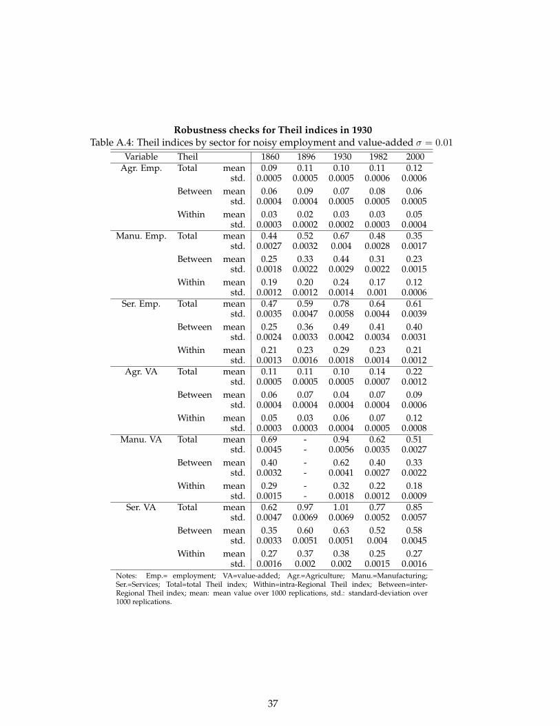
Robustness checks for Theil indices in 1930Table A.4: Theil indices by sector for noisy employment and value-added σ = 0.01

Variable Theil 1860 1896 1930 1982 2000Agr. Emp. Total mean 0.09 0.11 0.10 0.11 0.12

std. 0.0005 0.0005 0.0005 0.0006 0.0006Between mean 0.06 0.09 0.07 0.08 0.06

std. 0.0004 0.0004 0.0005 0.0005 0.0005Within mean 0.03 0.02 0.03 0.03 0.05

std. 0.0003 0.0002 0.0002 0.0003 0.0004Manu. Emp. Total mean 0.44 0.52 0.67 0.48 0.35

std. 0.0027 0.0032 0.004 0.0028 0.0017Between mean 0.25 0.33 0.44 0.31 0.23

std. 0.0018 0.0022 0.0029 0.0022 0.0015Within mean 0.19 0.20 0.24 0.17 0.12

std. 0.0012 0.0012 0.0014 0.001 0.0006Ser. Emp. Total mean 0.47 0.59 0.78 0.64 0.61

std. 0.0035 0.0047 0.0058 0.0044 0.0039Between mean 0.25 0.36 0.49 0.41 0.40

std. 0.0024 0.0033 0.0042 0.0034 0.0031Within mean 0.21 0.23 0.29 0.23 0.21

std. 0.0013 0.0016 0.0018 0.0014 0.0012Agr. VA Total mean 0.11 0.11 0.10 0.14 0.22

std. 0.0005 0.0005 0.0005 0.0007 0.0012Between mean 0.06 0.07 0.04 0.07 0.09

std. 0.0004 0.0004 0.0004 0.0004 0.0006Within mean 0.05 0.03 0.06 0.07 0.12

std. 0.0003 0.0003 0.0004 0.0005 0.0008Manu. VA Total mean 0.69 - 0.94 0.62 0.51

std. 0.0045 - 0.0056 0.0035 0.0027Between mean 0.40 - 0.62 0.40 0.33

std. 0.0032 - 0.0041 0.0027 0.0022Within mean 0.29 - 0.32 0.22 0.18

std. 0.0015 - 0.0018 0.0012 0.0009Ser. VA Total mean 0.62 0.97 1.01 0.77 0.85

std. 0.0047 0.0069 0.0069 0.0052 0.0057Between mean 0.35 0.60 0.63 0.52 0.58

std. 0.0033 0.0051 0.0051 0.004 0.0045Within mean 0.27 0.37 0.38 0.25 0.27

std. 0.0016 0.002 0.002 0.0015 0.0016Notes: Emp.= employment; VA=value-added; Agr.=Agriculture; Manu.=Manufacturing;Ser.=Services; Total=total Theil index; Within=intra-Regional Theil index; Between=inter-Regional Theil index; mean: mean value over 1000 replications, std.: standard-deviation over1000 replications.

37

Table A.5: Theil indices by sector for noisy employment and value-added σ = 0.10

Variable Theil 1860 1896 1930 1982 2000Agr. Emp. Total mean 0.10 0.12 0.10 0.12 0.12

std. 0.0049 0.0048 0.0051 0.0056 0.0062Between mean 0.06 0.09 0.07 0.08 0.06

std. 0.004 0.0042 0.0047 0.0052 0.0047Within mean 0.04 0.03 0.03 0.04 0.06

std. 0.0029 0.0026 0.0025 0.0028 0.004Manu. Emp. Total mean 0.44 0.53 0.68 0.48 0.35

std. 0.0273 0.0322 0.0398 0.0283 0.0171Between mean 0.25 0.33 0.44 0.31 0.23

std. 0.0177 0.0224 0.0286 0.0219 0.0146Within mean 0.19 0.20 0.24 0.17 0.13

std. 0.0115 0.0122 0.0141 0.0096 0.0065Ser. Emp. Total mean 0.47 0.59 0.78 0.65 0.61

std. 0.0354 0.0474 0.0583 0.0442 0.0386Between mean 0.25 0.36 0.49 0.41 0.40

std. 0.0241 0.033 0.0422 0.0337 0.0309Within mean 0.22 0.23 0.29 0.24 0.21

std. 0.013 0.0159 0.0179 0.0135 0.0116Agr. VA Total mean 0.11 0.11 0.11 0.15 0.22

std. 0.0051 0.005 0.0051 0.0072 0.0115Between mean 0.06 0.08 0.04 0.07 0.09

std. 0.0044 0.0042 0.0037 0.0043 0.0057Within mean 0.05 0.04 0.06 0.08 0.13

std. 0.0032 0.0029 0.0039 0.0048 0.0079Manu. VA Total mean 0.70 - 0.94 0.62 0.51

std. 0.0452 - 0.0562 0.0348 0.0264Between mean 0.40 - 0.63 0.40 0.33

std. 0.0315 - 0.0412 0.0267 0.0218Within mean 0.29 - 0.32 0.22 0.18

std. 0.0154 - 0.0179 0.0117 0.009Ser. VA Total mean 0.62 0.97 1.01 0.77 0.85

std. 0.0467 0.0693 0.0689 0.0519 0.057Between mean 0.35 0.60 0.63 0.52 0.58

std. 0.0328 0.0507 0.0511 0.0402 0.0448Within mean 0.27 0.37 0.38 0.25 0.27

std. 0.0159 0.0204 0.0198 0.015 0.016Notes: Emp.= employment; VA=value-added; Agr.=Agriculture; Manu.=Manufacturing;Ser.=Services; Total=total Theil index; Within=intra-Regional Theil index; Between=inter-Regional Theil index; mean: mean value over 1000 replications, std.: standard-deviation over1000 replications.

38

Res

ults

ofth

efir

st-s

tage

regr

essi

ons

Tabl

eA

.6:I

ndus

try-

spec

ific

prod

ucti

vity

and

dens

ity,

first

-sta

gere

gres

sion

s(P

ool.)

(186

0)(1

930)

(200

0)D

epen

dent

var.

lnden

dt

lnMPdt

lnden

dt

lnMPdt

lnden

dt

lnMPdt

lnden

dt

lnMPdt

lnden

d1801

1.39a

-0.0

3c1.

24a

-0.0

21.

45a

-0.0

31.

31a

-0.0

5b

(0.1

1)(0

.02)

(0.0

7)(0

.01)

(0.1

2)(0

.02)

(0.1

6)(0

.02)

lnMPd1801

-0.6

21.

72a

-0.8

7a1.

09a

-1.1

6b1.

85a

0.61

2.22a

(0.4

9)(0

.16)

(0.2

4)(0

.07)

(0.5

1)(0

.17)

(0.5

2)(0

.16)

lnav.distancedt

-0.3

10.

59a

-0.8

2a0.

06-0

.84c

0.68a

0.28

0.92a

(0.4

8)(0

.12)

(0.2

7)(0

.05)

(0.5

0)(0

.13)

(0.5

0)(0

.12)

lnaread

-0.2

5c0.

03-0

.21b

0.02

-0.3

3c0.

040.

030.

04(0

.15)

(0.0

2)(0

.09)

(0.0

1)(0

.18)

(0.0

2)(0

.17)

(0.0

3)lndivdt

-0.6

8a-0

.07c

-0.1

4-0

.004

0.33

0.20a

-4.2

3a-0

.48a

(0.1

4)(0

.04)

(0.1

0)(0

.02)

(0.2

7)(0

.05)

(0.5

5)(0

.12)

Year

fixed

-eff

ect

Yes

Yes

No

No

No

No

No

No

N26

126

187

8787

8787

87Sh

ea’s

part

ialR

20.

645

0.87

90.

852

0.97

00.

709

0.91

50.

616

0.85

3N

otes

:(i)

Rob

usts

tand

ard

erro

rsin

brac

kets

;a,b

andc

are

sign

ifica

nce

leve

lsat

the

1%,5

%an

d10

%th

resh

-ol

ds,r

espe

ctiv

ely.

39

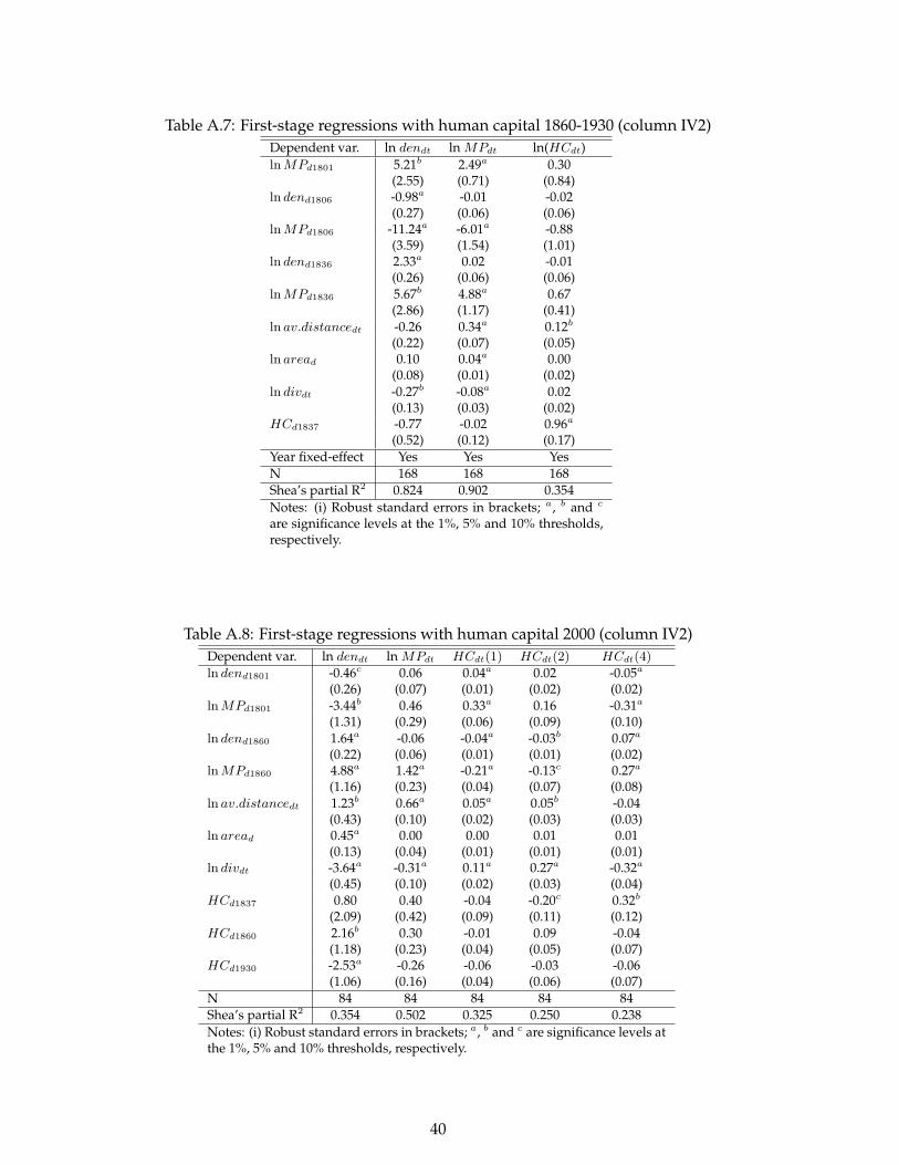
Table A.7: First-stage regressions with human capital 1860-1930 (column IV2)Dependent var. ln dendt ln MPdt ln(HCdt)lnMPd1801 5.21b 2.49a 0.30

(2.55) (0.71) (0.84)ln dend1806 -0.98a -0.01 -0.02

(0.27) (0.06) (0.06)lnMPd1806 -11.24a -6.01a -0.88

(3.59) (1.54) (1.01)ln dend1836 2.33a 0.02 -0.01

(0.26) (0.06) (0.06)lnMPd1836 5.67b 4.88a 0.67

(2.86) (1.17) (0.41)ln av.distancedt -0.26 0.34a 0.12b

(0.22) (0.07) (0.05)ln aread 0.10 0.04a 0.00

(0.08) (0.01) (0.02)ln divdt -0.27b -0.08a 0.02

(0.13) (0.03) (0.02)HCd1837 -0.77 -0.02 0.96a

(0.52) (0.12) (0.17)Year fixed-effect Yes Yes YesN 168 168 168Shea’s partial R2 0.824 0.902 0.354Notes: (i) Robust standard errors in brackets; a, b and c

are significance levels at the 1%, 5% and 10% thresholds,respectively.

Table A.8: First-stage regressions with human capital 2000 (column IV2)Dependent var. ln dendt ln MPdt HCdt(1) HCdt(2) HCdt(4)

ln dend1801 -0.46c 0.06 0.04a 0.02 -0.05a

(0.26) (0.07) (0.01) (0.02) (0.02)lnMPd1801 -3.44b 0.46 0.33a 0.16 -0.31a

(1.31) (0.29) (0.06) (0.09) (0.10)ln dend1860 1.64a -0.06 -0.04a -0.03b 0.07a

(0.22) (0.06) (0.01) (0.01) (0.02)lnMPd1860 4.88a 1.42a -0.21a -0.13c 0.27a

(1.16) (0.23) (0.04) (0.07) (0.08)ln av.distancedt 1.23b 0.66a 0.05a 0.05b -0.04

(0.43) (0.10) (0.02) (0.03) (0.03)ln aread 0.45a 0.00 0.00 0.01 0.01

(0.13) (0.04) (0.01) (0.01) (0.01)ln divdt -3.64a -0.31a 0.11a 0.27a -0.32a

(0.45) (0.10) (0.02) (0.03) (0.04)HCd1837 0.80 0.40 -0.04 -0.20c 0.32b

(2.09) (0.42) (0.09) (0.11) (0.12)HCd1860 2.16b 0.30 -0.01 0.09 -0.04

(1.18) (0.23) (0.04) (0.05) (0.07)HCd1930 -2.53a -0.26 -0.06 -0.03 -0.06

(1.06) (0.16) (0.04) (0.06) (0.07)N 84 84 84 84 84Shea’s partial R2 0.354 0.502 0.325 0.250 0.238Notes: (i) Robust standard errors in brackets; a, b and c are significance levels atthe 1%, 5% and 10% thresholds, respectively.

40