the spectral correlation function – a new tool for ... · pdf filethe spectral...
TRANSCRIPT
arX
iv:a
stro
-ph/
9903
454v
2 2
0 A
pr 1
999
The Spectral Correlation Function –
A New Tool for Analyzing Spectral-Line Maps
Erik W. Rosolowsky1, Alyssa A. Goodman2 3, David J. Wilner4 5 and Jonathan P.
Williams6
Harvard-Smithsonian Center for Astrophysics, 60 Garden Street, Cambridge, MA 02138.
Revised for The Astrophysical Journal, Part I, March 1999
Received ; accepted
[email protected], Swarthmore College
3National Science Foundation Young Investigator
5Hubble Fellow
– 2 –
ABSTRACT
The “spectral correlation function” analysis we introduce in this paper is a
new tool for analyzing spectral-line data cubes. Our initial tests, carried out
on a suite of observed and simulated data cubes, indicate that the spectral
correlation function [SCF] is likely to be a more discriminating statistic than
other statistical methods normally applied. The SCF is a measure of similarity
between neighboring spectra in the data cube. When the SCF is used to
compare a data cube consisting of spectral-line observations of the ISM with
a data cube derived from MHD simulations of molecular clouds, it can find
differences that are not found by other analyses. The initial results presented
here suggest that the inclusion of self-gravity in numerical simulations is critical
for reproducing the correlation behavior of spectra in star-forming molecular
clouds.
Subject headings: ISM: structure—line: profiles—(magnetohydrodynamics:)
MHD—methods: data analysis—molecular data—turbulence

– 3 –
1. Introduction
The “spectral correlation function” analysis we introduce in this short paper is a new
tool for analyzing spectral-line data cubes. Owing to the recent advances in receiver and
computer technology, both observed and simulated cubes have been growing in size. Our
ability to intuit their import, however, has not kept pace. Therefore, the need for statistical
methods of analyzing these cubes has now become acute.
Several methods for analyzing spectral-line data cubes have been proposed and applied
over the past fifteen years. Many of the methods are “successful” in that they can describe
a cube with far fewer bits than the original data set contained. The question in the study
this paper introduces can be phrased as “just which bits describe the cube most uniquely?”
In particular, we seek a method which produces easily understood results, but preserves
as much information as possible about all of the dimensions of a position-position-velocity
cube of intensity measurements.
Some previous statistical analyses do not explicitly make use of the velocity dimension
in analyzing spectral-line cubes. For example, Gill and Henriksen (1990) and Langer,
Wilson, & Anderson (1993) apply wavelet analysis to position-position-intensity data, in
order to represent the physical distribution of material in a mathematically efficient way.
Houlahan and Scalo (1992) use structure-tree statistics on IRAS images to analyze the
hierarchical vs. random nature of molecular clouds, ultimately finding evidence for some of
each. Wiseman and Adams (1994) use pseudometric methods on IRAS data to describe
and rank cloud “complexity.” Elmegreen and Falgarone (1996) analyze the clump mass
spectrum of several molecular clouds in order to determine a characteristic fractal dimension
for the star-forming interstellar medium. Blitz and Williams (1997) find evidence for a
break in the column density distribution of material in clouds by analyzing histograms of
column density.

– 4 –
Other analyses preserve velocity information along with the spatial information in
analyzing the cubes. At present, these kinds of analyses can essentially be broken down
into two groups.
In the first group, no transforms are taken, and spatial information is preserved
directly. For example Williams, de Geus, & Blitz (1994) use the CLUMPFIND program,
and Stutzki & Gusten (1990) use their GAUSSCLUMPS algorithm to identify “clumps” in
position-position-velocity space. Statistical analyses are made on the distributions of clump
properties (e.g. the clump mass spectrum is calculated) to probe the three dimensional
structure of molecular clouds.
In the second group, transforms of one kind or another are performed, and spatial
information is preserved as “scale” rather than as “position” information. The classic
example of this kind of analysis involves calculation of autocorrelation and structure
functions. Application of these functions to molecular cloud data was first suggested by
Scalo (1984) and then applied to real data by Kleiner and Dickman (1985) and by Miesch
and Bally (1994). Heyer and Schloerb (1994) have recently applied Principal Components
Analysis (PCA) to several data cubes. This method describes clouds as a sum of special
functions in a manner mathematically similar to wavelet analysis. Most of these analyses
have offered new insights into cloud structure and kinematics.
Using this breakdown, the SCF falls into the first group,7 in that no transforms are
7Strictly speaking, the SCF is in the first group when applied for a fixed spatial resolution.
However, the SCF can be used as a tool more like the autocorrelation function analyses
mentioned in the second group, by comparing runs with different spatial resolution. An
upcoming paper (Padoan & Goodman 1999) discusses the effects of varying the ratio of
resolution to map size on the SCF (see §3.4).

– 5 –
performed and spatial information is preserved directly. The SCF simply describes the
similarities in shape, size, and velocity offset among neighboring spectra in a data cube. In
originally developing the SCF, our goal was to create a “hard-to-fool” statistic for use in
comparing data cubes calculated from simulations of the ISM with those of observed cubes.
The exact reproduction of an observed object in the ISM through simulation is
practically impossible so simulations need to be evaluated on their ability to reproduce more
general properties of the ISM like appropriate scaling relationships. In the only published
work known to us8 that specifically evaluates hydrodynamic simulations by comparing
them with real spectral maps, Falgarone et al. (1994) have compared a simulation by
Porter, Pouquet & Woodward (1994) with an observed data cube (See also the analysis of
simulated cubes in Dubinski, Narayan & Phillips 1995). The observed cube is a CO map
of a small piece of the expanding H I loop in Ursa Major, first mapped by Heiles (1976).
The Falgarone et al. (1994) analysis is based on comparing combinations of the moments of
the the derived distributions of spectral line parameters for each cube. They find that the
moment analysis on the observed maps agrees well with one performed on the simulations.
We show, below, however, that this comparison may not have been strict enough, in that
the distribution of the SCF for the Porter et al. (1994) simulation differs significantly from
the distribution calculated for the observed Ursa Major data cube.
8Padoan et al. 1999 have recently submitted a comparison of the Padoan & Nordlund
(1999) simulations with 13CO maps of the Perseus Molecular Cloud to the Astrophysical
Journal. The cubes are compared using moments of the distribution of line parameters (see
§3.5).
– 6 –
2. The SCF Algorithm
The SCF project was developed in order to probe the nature of correlation in spectral-
line maps of molecular clouds. Unlike other probes like Scalo’s (1984) Autocovariance
Function (ACF) and Structure Function (SF), the SCF is specifically designed to preserve
detailed spatial information in spectral-line data cubes. The motivations and mathematical
background of the project are discussed in Goodman (1997).
2.1. The Development of the SCF
The SCF algorithm centers around quantifying the differences between spectra. To
begin, a deviation function, D, is defined which represents the differences between two
spectra, T1(v) and T0(v).
D(T1, T0) ≡ mins,ℓ
{∫
[s · T1(v − ℓ)− T0(v)]2 dv
}
(1)
The two parameters s and ℓ are included in the function so differences in height and velocity
offset between the two spectra can be eliminated, recognizing similarities solely in the shape
of two line profiles. These parameters can be adjusted in order to find the scaling and/or
velocity-space shifting which minimizes the differences between the spectra. In addition,
the deviation function can be evaluated with either or both of the parameters fixed.
We normalize the deviation function to the unit interval: a value of 1 indicating
identical spectra and a value of 0 indicating minimal correlation9. The appropriate
normalization is to divide by the maximum value of the deviation function in the absence
of absorption and subtract this value from 1. The resulting function is referred to as the
9A value of 1 can only be achieved in the case of infinite signal to noise. See §2.2
– 7 –
SCF evaluated for the two spectra.
S(T1, T0) ≡ 1−
√
√
√
√
D(T1, T0)
s2∫
T 21 (v)dv +
∫
T 20 (v)dv
(2)
As mentioned previously, the deviation function can be evaluated with the parameters s or
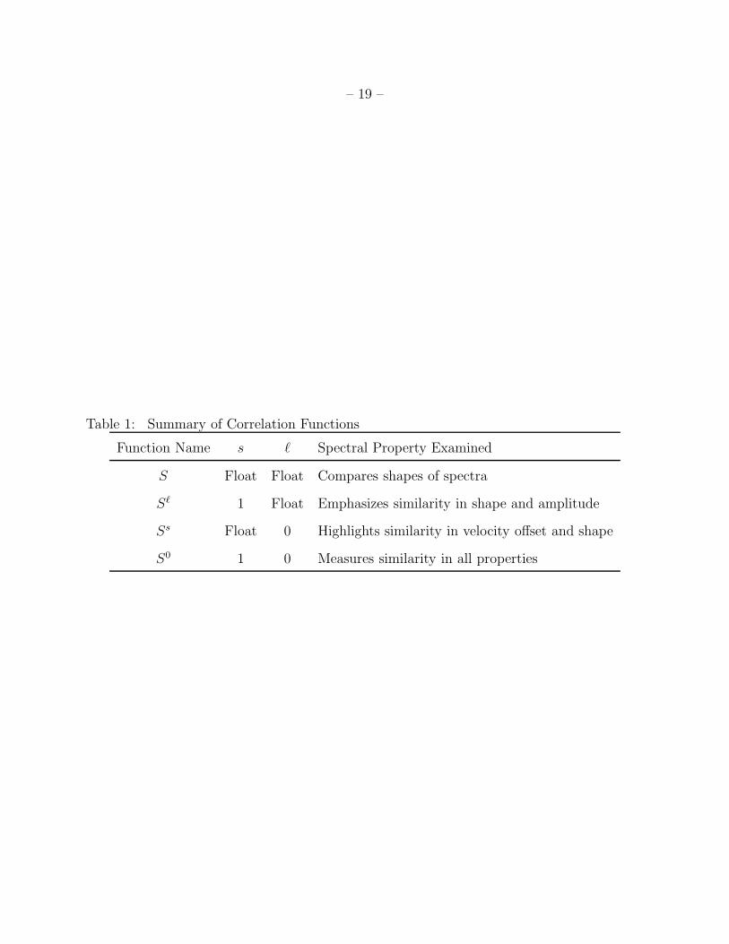
ℓ fixed, to 1 and/or 0, respectively. Such restrictions provide different kinds of information
about the two spectra under examination. The resulting forms of the spectral correlation
function are summarized in Table 1.
In order to examine spectral-line maps, comparison of two spectra must be extended to
the analysis of many spectra simultaneously. The simplest such extension is to evaluate the
functions S, Sℓ, Ss and S0 between a base spectrum and each spectrum in the map within
a specified angular range from the base spectrum. We refer to the angular range under
consideration as the resolution of the SCF. All of the SCF calculations are performed using
only the central portion of the spectra, specifically, over a range equal to a given number
of FWHMs of the base spectrum from each spectrum’s velocity centroid. The FWHM is
defined by a Gaussian fit to the base spectrum’s line profile.10 The resulting values of the
SCF are then averaged together with the option of weighting the results based on distance
from the original spectrum. The averaged value is the correlation of the base spectrum with
10The Gaussian fit is only used to set a reasonable window over which the SCF is calculated.
For very noisy data, including extra baseline decreases the SCF. The line profiles discussed
in this paper are all roughly gaussian, with widths that do not vary much within a map,
so the change in the SCF caused by varying window size is tiny. However, in other cases,
such as analysis of H I line profiles, a window must be manually set, and fixed, as Gaussian
fitting gives spurious widths. A new version of the SCF, developed to deal with H I data,
uses a fixed spectral window and is presented in Ballesteros-Paredes, Vazquez-Semadeni &
Goodman 1999.

– 8 –
its neighbors and a similar analysis is then performed for every spectrum in the map. When
the SCF is evaluated for neighboring points in the spectral-line map, the averages use many
of the same spectra, implying that SCF values for points within an SCF resolution element
are not independent.
2.2. The Effects of Instrumental Noise
Our measure of the similarity between observed spectra must deal with the effects
of noise. Noise obscures similarities and differences between the two spectra under
examination, usually skewing the results to indicate less correlation than is actually present.
Hence, the principal difficulty generated by noise is that it creates a bias in correlation
measurements, favoring spectra with higher values of signal-to-noise.
We have explored a few methods of subtracting out noise bias using techniques shown
to work on infinitely well-sampled data. However, these techniques break down for data
with limited resolution (Rosolowsky 1998). While highly unconventional, we have found
that the best method of dealing with non-uniform signal-to-noise is to discard all spectra
with signal-to-noise below a certain cutoff value, (TA/σ)c, and then to add normally
distributed random noise to spectra with signal-to-noise greater than the cutoff until all
spectra have TA/σ = (TA/σ)c. This method appears effective because it eliminates the bias
(See Figure 1) and the resulting correlation outputs do not appear to depend strongly on
specific set of noise added. The maximum value of the SCF cannot reach 1 for any finite
value of TA/σ; instead, the maximum is dependent on the line shape and the cutoff value for
the signal-to-noise. Figure 2 depicts the rise in SCF values with increasing signal-to-noise
for each of the correlation functions. These data are generated by using the SCF to analyze
a data cube consisting of identical Gaussian spectra which have had noise added to achieve
a specific value of (TA/σ)c.
– 9 –
We considered renormalizing the SCF by a factor equal to the inverse of the maximum
SCF possible for the (TA/σ)c used. If we did so then absolute SCF values would always
have the same meaning. However, since the exact maximum possible depends on line
shape, we chose not to renormalize. Instead, we note that whenever (TA/σ)c is set to the
same value, the maximum possible SCF value should be roughly equal for any cube. In the
examples below, we set (TA/σ)c = 5, which implies a maximum possible SCF of order 0.65
(See Figure 2).
This “noise equalizing” procedure may seem distasteful to some–especially to observers
who spend long hours at the telescope! The best way we can explain its necessity is by
reminding the reader that you cannot get something for nothing. In other words, if your
data is noisy, you simply cannot know how well correlated two spectra are as well as if the
spectra were clean. Uncorrelated noisy spectra can look just the same as correlated noisy
spectra. Any correction introduces different amounts of uncertainty for different positions in
the map. For this reason, until someone makes a better proposal, we continue to advocate
equalizing signal to noise at a threshold value.
3. First Results from the SCF
In this section, we analyze five sample data cubes chosen to demonstrate the SCF’s
ability to discriminate among different physical conditions. First, we describe the data
cubes (see Table 2), and then we discuss comparisons amongst them in the context of the
SCF. Of the two observational data cubes, one is for a self-gravitating cloud (Heiles Cloud
2), and one is for a non-self-gravitating high-latitude cloud (in Ursa Major). For the three
cubes generated from simulations: one is purely hydrodynamic and non-self-gravitating; one
is magnetohydrodynamic and non-self-gravitating; and the last is magnetohydrodynamic
and self-gravitating.
– 10 –
3.1. Data Sets
Heiles Cloud 2: In 1996, observers at FCRAO mapped Heiles Cloud 2 in the C18O(2 − 1)
line (deVries et al. 1999). The resulting data cube consists of 4800 spectra arranged in
a grid of 50 × 96 pixels on the sky. The grid covers 58′ in right ascension and 40′ in
declination, centered at α(2000) = 4h36m09s and δ(2000) = 25◦47′30′′. Assuming the cloud
is 140 pc distant, the map covers a physical area of 2.3 × 1.6 pc at a spatial resolution of
0.034 pc. The spectra have 256 channels of velocity running from -0.35 km/s to 12.45 km/s,
with a channel width of 0.05 km/s. The peak emission from the cloud is at about +6 km/s.
Ursa Major: The 12CO (2-1) map analyzed here is described in Falgarone et al. 1994. The
area mapped is located on a giant H I loop, and is claimed by Falgarone et al. to be “a good
site to study turbulence in molecular clouds given its proximity to an important source of
kinetic energy (the expanding loop itself).” The size of this map is 9 by 19 pixels, with a
grid step of 30′′ (0.015 pc if the cloud is at 100 pc). Note that there are approximately 50%
more pixels in the Porter et al. simulation than in this relatively small map.
Pure Hydrodynamic Turbulence: This cube, presented in presented in Porter et al. (1994),
is the one compared with the 12CO (2-1) Ursa Major data cube (see above) by Falgarone
et al. (1994). It is a three-dimensional simulation with periodic boundary conditions, no
magnetic fields, no gravity, and fully compressible turbulence. The time step analyzed here
is the second cube (t = 1.2τac) presented in Falgarone et al. (1994).
The spectra in the simulated data cube are laid out in a grid of 16× 16 pixels.11 There
are 512 channels in each spectrum and the channel width is 0.13 km/s. The simulated
spectra are generated from density-weighted histograms of velocity, which are intended to
11The full Porter et al. 1994 simulation is 5123, but the grid of 16×16 spectra is generated
by considering subsamples of the cube with dimensions 32× 32× 512.

– 11 –
mimic observations of the 12CO(2-1) line. The overall physical size of the simulation is not
given, but the nature of comparison with the CO map of Ursa Major shown in Falgarone et
al. (1994) implies that the spatial resolution of the simulated spectral-line map should be
approximately 0.015 pc (30′′ at 100 pc).
Magnetohydrodynamic Turbulence: Mac Low et al. (1998) have made their simulated cube
“L,” which represents uniform, isotropic, isothermal, supersonic, super-Alfvnic, decaying
turbulence available to us and others through the world wide web. The spectra are produced
as density-weighted histograms from a simulation using a finite-difference method (ZEUS;
see Stone & Norman 1992) and 2563 zones. Mac Low et al. use this cube, and others, to
study the free decay of turbulence in the ISM. Mac Low et al.’s results concerning decay
times apparently agree with those of Padoan & Nordlund (1999), who have carried out
equivalent simulations. The physical scale the Mac Low et al. cube represents depends
on the choice of other paramenters (e.g. field strength), but it is fair to estimate that the
resolution should be similar to that of Gammie et al (1999; see below), or about 0.06 pc.
Self-Gravitating Magnetohydrodynamic Turbulence: Another group, whose most recently
published work is Stone, Ostriker, & Gammie (1998), has been using the ZEUS code to
study self-gravitating MHD turbulence. Charles Gammie has kindly provided us with a
preliminary simulated spectral-line cube with dimensions 32 × 32 × 256, generated from
a recent 3D, self-gravitating, high-resolution run (Gammie et al. 1999). The spectra are
density-weighted histograms meant to simulate 13CO emission, observed with a velocity
resolution of 0.054 km s−1. As is the case for the Porter et al. (1994) simulations presented
in Falgarone et al. (1994), the larger original (here, 2563) simulation is downsampled in
the two spatial dimensions (here to 32 × 32) to produce reasonable spectra. The resulting
spatial resolution is approximately 0.06 pc.

– 12 –
3.2. Analysis
For all of the SCF analyses presented in this paper, the cutoff signal-to-noise ratio is
set to 5, the spatial resolution of the SCF includes all spectra within 2 pixels of the base
spectrum, uniform weighting is applied across the resolution element, and the portion of
each spectrum within 3 base spectrum FWHMs of the velocity centroid is used.
For each data cube, greyscale maps of the SCF values are generated and compared
with maps of line parameters such as antenna temperature. Note that before the noise
correction discussed in §2.2 was applied, maps of the peak antenna temperature TA and the
SCF looked similar. After correction, this is no longer the case. So, the greyscale maps
of the SCF, which preserve all the spatial information about which spectra in a map are
correlated, can be informative on their own. In addition to pointing out correlations with
various line parameters, they are highlight edges of H I shells (see Ballesteros-Paredes,
Vazquez-Semadeni & Goodman 1999) and other such structures. In the current paper,
however, we show only simple histograms (Figure 3) of all of the values of the SCF in a
map, which are easier to quantitatiely intercompare than the greyscale images. We present
a moment analysis of these distributions in Table 3.
As a test of the hypothesis that the positions of spectra within a cube are important
to its description, we calculate the SCF for the original cubes and for “comparison” cubes
where the positions are randomized. If the meaning of the SCF is linked to the original
positions of the spectra, randomization of the positions should create a significant change
in the SCF values. This drop is in fact observed in our analysis. The magnitude of the drop
depends on the cube being analyzed and the compensatory parameters used in the SCF
but not on the specific randomized positions. Different randomizations produce changes
of ∼ 1% in the mean values of correlation functions. The SCF results for the randomized
cubes appear with the original histograms and moment analysis (Figure 3 and Table 3).

– 13 –
The significance of the drop in the mean value of the SCF caused by randomization is
high in all cases studied here. The error in estimating the mean in each SCF distribution is
of order the standard deviation of the distribution divided by√
Npixels × 3∆vchannels, where
Npixels is the number of pixels in the map and 3∆vchannels is the number of spectral channels
considered in calculating the SCF. As can be seen from Tables 2 and 3, the standard
deviations of the distributions are all less than 0.1, and the minimum√
Npixels × 3∆vchannels
is of order 5 × 10³, meaning that the error in the quoted mean is always less than about
1 × 10⁻³. This value is much smaller than any of the differences between SCF means for
actual and randomized maps listed in the last column of Table 3.
3.3. Inferences
The most basic conclusion we draw from our analysis is that the SCF does recognize
some form of spectral correlation in data cubes. The drop in the mean and increased spread
in the distribution when positions are randomized depicts a clear loss of spatial correlation
of the spectra. When the compensatory parameters s and ℓ are fixed, the difference between
the two histograms becomes clearer because the program has fewer tools to compensate for
the differences in the spectra. For example, in Heiles Cloud 2, randomization causes the
smallest correlation drop when both the lag and scaling parameters are allowed to vary,
indicating that the spectra are similar in shape throughout the data cube. The fact that
the mean value of Sℓ is larger than that of Ss implies that the spectra in the cube are more
similar in overall antenna temperature than in velocity distribution. In other words, it
appears that the compensatory parameter ℓ is more important for good correlation than is
the scaling parameter s in this case.
Examining Figure 3 and Table 3 closely, one can detect a clear pattern. From this set
of examples, it appears that the more gravity matters, the more of an effect randomization
– 14 –
has on the SCF distribution. The SCF distribution for the self-gravitating cloud (Heiles
Cloud 2) shows a much larger change in response to randomization in spectral positions
than does the unbound high-latitude cloud (Ursa Major). The simulation which most
closely reflects the Heiles Cloud 2 response to randomization is the only one that includes
self-gravity: Gammie et al. (1999). In the non-self-gravitating case, the Ursa Major SCF
distributions show much less change in response to randomization than the Heiles Cloud
2 distributions, but more change than the distributions for the simulations presented as
their “match” in Falgarone et al. 1994 (see Table 3). This trend is corroborated by a visual
inspection of the grid of simulated spectra (Falgarone et al. 1994 Figure 1b), where it is
seen that the differences between neighboring spectra appear more pronounced than in the
Ursa Major observations. Such behavior indicates that the original positions of the spectra
in the simulated cube are not as essential to the cloud description as they are in Ursa Major.
As for the mean values of the SCF, it is acceptable to intercompare means for the
five data sets used here because signal-to-noise values have been equalized (see §2.2). The
SCF means for the Mac Low et al. (1998) simulations seem the best match to the Heiles
Cloud 2 data. The means for the simulation presented in Falgarone et al. 1994 are not very
similar to those for the Ursa Major cloud which Falgarone et al. claim is an excellent match
for these simulations. In particular, the means for S and Sℓ in the simulation are nearly
equal (0.6) as are those for Ss and S0 (0.52), meaning that lag adjustments are important,
but scale adjustments are not. In the Ursa Major observations, all forms of the SCF give
roughly 0.55, and this difference between lag and scaling is not seen.
3.4. Resolution and Sampling Effects
If two maps of similar regions have very different spatial resolution, the map with lower
resolution will look smoother. One can imagine that the spectra in the lower resolution

– 15 –
map will change more rapidly from one position to the next, so that the mean SCF for
the lower resolution map will be lower if the SCF is run with the same size averaging
box. Alternatively, one can imagine running the SCF with a very large averaging box on a
high-resolution map, thus “smearing out” small differences in spectra that might show up
in a smaller box.
To investigate issues of resolution, we have used the Heiles Cloud 2 data set in a
numerical experiment. We re-ran the SCF many times, using a box size of 3 (the original),
5, 7, 9, 11, 13, and 15 pixels, to see what effect this “smoothing” would have on the SCF.
Figure 4 presents the results of this experiment.
The mean value of the SCF in Heiles Cloud 2 does drop for larger box sizes, but by
a surprisingly small amount (see Figure 4). (For the Heiles Cloud 2 cube with positions
randomized, the SCF is unaffected by changes in resolution, as expected.) The width of the
SCF distributions for Heiles Cloud 2 with positions randomized also drops a bit for larger
box sizes, illustrating that small spectral differences do eventually get smeared-out, even
when spectra are shuffled. Thus, for this one example, the effect of changing resolution is
relatively small.
Other factors can also effect the true resolution–and resulting magnitude–of the
SCF. The way the spectra in a map are sampled will effect the absolute values of the
SCF measured. For example, in a Nyquist-sampled map, neighboring spectra are not
independent and will necessarily yield higher values of the SCF than a beam-sampled map.
In this paper, we have tried to restrict ourselves to beam-sampled maps, but a correction
for sampling should be added to the SCF algorithm in the future.
Ultimately, it is the relationship between map resolution, averaging box size, map size,
and physically important scales (e.g. Alfven wave cutoff, outer scale of turbulence, Jeans
length, etc.) that determine the SCF. The subtleties of these relationships’ influence on the

– 16 –
SCF, and on other statistical techniques, are discussed in Padoan & Goodman 1999.
3.5. How discriminating is the SCF?
This paper is intended as a “proof-of-concept,” to show that the SCF is a discriminating
tool for analyzing observed and simulated spectral-line maps. As discussed in the previous
section, Falgarone et al. (1994) concluded that the simulated cube of Porter et al. 1994 is an
extraordinary match to the 12CO(2-1) observations of Ursa Major. This conclusion is based
on Falgarone et al.’s analysis of combinations of statistical moments of distributions of
antenna temperatures. We have shown here that, contrary to Falgarone et al.’s conclusions,
the SCF can detect significant differences between these two data sets.
In addition, we have tested the SCF against the comparison method where the simple
histograms of moments (centroid velocity, velocity width, skewness, and kurtosis) of spectra
in a map are used to intercompare data cubes. It turns out that this seemingly simple
method has one major weakness. The values of the higher-order moments (skewness and
kurtosis) are extremely sensitive to how one treats noise in the data cube. Some researchers
(e.g. Padoan et al. 1999) choose to set a threshold of nσ (where n is usually 3 and σ is
the rms noise in a spectrum) before calculating moments. It turns out that the value of n
has profound effects on the skewness and kurtosis distributions for the whole cube. We also
compared equalizing the signal-to-noise in a cube and then computing moments. This gives
different results than thresholding. Given these complications, we reserve further discussion
of moment distribution comparisons for future work.
For now, based on the re-comparison of the data and simulation in Falgarone et al.
1994, we have shown that the SCF does find differences where other methods do not.

– 17 –
4. Conclusions
The drop to lower correlation values when spectral positions are randomized shows the
SCF is performing its primary function of quantifying the correlation between proximate
spectra in a data cube.
In this first paper, we have demonstrated that the SCF algorithm can find subtle
differences between simulated and observational data cubes that may not be evident in
other kinds of comparisons. Thus, application of the SCF will provide a “sharper tool” to
be used in comparing simulated and observational data cubes in the future. There is far
more information produced by the SCF algorithm than is presented here and the full extent
and import of the information provided will be explored in subsequent papers.
In the future, we plan to exploit the information generated by the SCF to examine a
large variety of observational and simulated data cubes. Ultimately, our aim is to use the
SCF to evaluate which physical conditions imposed on MHD simulations are necessary to
produce the correlations observed in the ISM. The initial results presented here, showing
stronger drops in spectral correlation in response to randomization in self-gravitating
situations, hint that including self-gravity may be essential in the numerical recreation of
star-forming regions. Physical effects other than gravity, such as large-scale shocks, should
also have an “organizing” effect on the spatial distribution of spectra, and we intend to
search for those effects with the SCF as well.
A deeper coverage of the development of the SCF is found in Rosolowsky (1998) which
is available on the internet12. The SCF algorithm is written in IDL and is available for
public use13.
12See http://cfa-www.harvard.edu/˜agoodman/scf/SCF/scfmain.html
13 http://cfa-www.harvard.edu/˜agoodman/scf/distribution/

– 18 –
We would like to thank Marc Heyer of FCRAO for the use of the Heiles Cloud 2 data
set prior to publication. We wish to express our thanks to Derek Lis who facilitated access
to the simulated and observed data in Falgarone et al. (1994). Uros Seljak provided some
clear insights into the effects of instrumental noise which have proved indispensable in
our understanding and we are grateful. Thanks are in order to Mordecai Mark Mac-Low
for providing access to his group’s MHD simulations. And, our gratitude extends to
Charles Gammie who allowed access to the MHD simulations of Gammie, Ostriker and
Stone. Analysis of these additional simulations is available at our web site. Javier
Ballesteros-Paredes provided valuable help with revisions to this paper. Finally, we are
most grateful to an anonymous referee whose comments very significantly improved the
integrity of this paper. This research is funded by grant AST-9721455 to A.G. from the
National Science Foundation.
– 19 –
Table 1: Summary of Correlation Functions
Function Name s ℓ Spectral Property Examined
S Float Float Compares shapes of spectra
Sℓ 1 Float Emphasizes similarity in shape and amplitude
Ss Float 0 Highlights similarity in velocity offset and shape
S0 1 0 Measures similarity in all properties
– 20 –
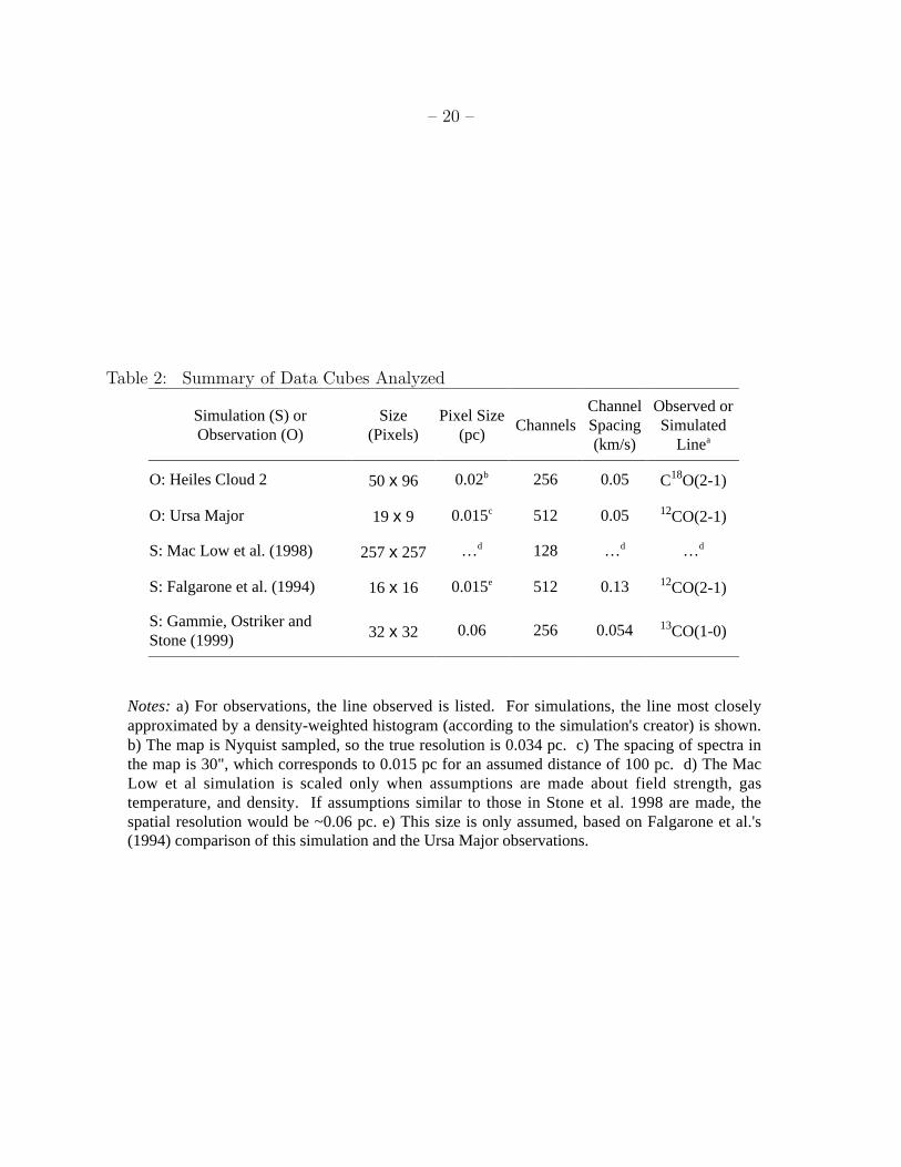
Table 2: Summary of Data Cubes Analyzed
Simulation (S) orObservation (O)
Size(Pixels)
Pixel Size(pc)
ChannelsChannelSpacing(km/s)
Observed orSimulated
Linea
O: Heiles Cloud 2 50 x 96 0.02b 256 0.05 C18O(2-1)
O: Ursa Major 19 x 9 0.015c 512 0.05 12CO(2-1)
S: Mac Low et al. (1998) 257 x 257 …d 128 …d …d
S: Falgarone et al. (1994) 16 x 16 0.015e 512 0.13 12CO(2-1)
S: Gammie, Ostriker andStone (1999) 32 x 32 0.06 256 0.054 13CO(1-0)
Notes: a) For observations, the line observed is listed. For simulations, the line most closelyapproximated by a density-weighted histogram (according to the simulation's creator) is shown.b) The map is Nyquist sampled, so the true resolution is 0.034 pc. c) The spacing of spectra inthe map is 30", which corresponds to 0.015 pc for an assumed distance of 100 pc. d) The MacLow et al simulation is scaled only when assumptions are made about field strength, gastemperature, and density. If assumptions similar to those in Stone et al. 1998 are made, thespatial resolution would be ~0.06 pc. e) This size is only assumed, based on Falgarone et al.'s(1994) comparison of this simulation and the Ursa Major observations.

– 21 –
Table 3: Statistical Outputs of the SCF
Heiles Cloud 2 (Star-forming Cloud)
Function Original Position Random Positions Difference
Mean Std. Deviation Mean Std. Deviation in Means
S 0.64 0.030 0.57 0.051 0.07
Sℓ 0.63 0.033 0.50 0.061 0.14
Ss 0.62 0.037 0.41 0.074 0.21
S0 0.62 0.036 0.39 0.070 0.23
Ursa Major (Unbound High-Latitude Cloud)
Function Original Position Randomized Positions Difference
Mean Std. Deviation Mean Std. Deviation in Means
S 0.55 0.10 0.49 0.09 0.05
Sℓ 0.56 0.09 0.49 0.08 0.07
Ss 0.54 0.10 0.42 0.09 0.12
S0 0.55 0.09 0.44 0.08 0.11
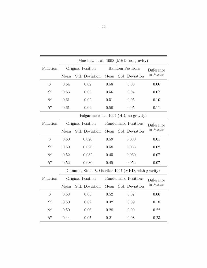
– 22 –
Mac Low et al. 1998 (MHD, no gravity)
Function Original Position Random Positions Difference
Mean Std. Deviation Mean Std. Deviation in Means
S 0.64 0.02 0.58 0.03 0.06
Sℓ 0.63 0.02 0.56 0.04 0.07
Ss 0.61 0.02 0.51 0.05 0.10
S0 0.61 0.02 0.50 0.05 0.11
Falgarone et al. 1994 (HD, no gravity)
Function Original Position Randomized Positions Difference
Mean Std. Deviation Mean Std. Deviation in Means
S 0.60 0.020 0.59 0.030 0.01
Sℓ 0.59 0.026 0.58 0.033 0.02
Ss 0.52 0.032 0.45 0.060 0.07
S0 0.52 0.030 0.45 0.052 0.07
Gammie, Stone & Ostriker 1997 (MHD, with gravity)
Function Original Position Randomized Positions Difference
Mean Std. Deviation Mean Std. Deviation in Means
S 0.58 0.05 0.52 0.07 0.06
Sℓ 0.50 0.07 0.32 0.09 0.18
Ss 0.50 0.06 0.28 0.09 0.22
S0 0.44 0.07 0.21 0.08 0.23

– 23 –
REFERENCES
Blitz, L. & Williams, J. 1997, ApJL, 488, L145
deVries, C., Ladd, E., Heyer, M., & Snell, R. 1999, ApJ, In Preparation
Dubinski, J., Narayan, R., & Phillips, T. 1995, ApJ, 448, 226
Elmegreen, B. G. & Falgarone, E. 1996, ApJ, 471, 816
Falgarone, E., Lis, D., Phillips, T., Pouquet, A., Porter, D., & Woodward, P. 1994, ApJ,
436, 728
Gammie, C., Ostriker, E. & Stone, J. 1999, personal communication.
Gill, A. G. & Henriksen, R. N. 1990, ApJL, 365, L27
Goodman, A. A. 1997, http://cfa-www.harvard.edu/∼agoodman/scf/scf.pdf
Heiles, C. 1976, ApJ, 208, 137
Heyer, M. H. & Schloerb, F. P. 1997, ApJ, 475, 173
Houlahan, P. & Scalo, J. 1992, ApJ, 393, 172
Kleiner, S. & Dickman, R. 1985, ApJ, 295, 456
Langer, W., Wilson, R., & Anderson, C. 1993, ApJL, 408, L25
Mac Low, M.-M., Klessen, R.S., Burkert, A. & Smith, M.D. 1998, PhysRevL, 80, 2754
Meisch, M. & Bally, J. 1994, ApJ, 429, 645
Padoan, P., Bally, J., Billawalla, Y., Juvela, M. & Nordlund, A. 1999, ApJ, submitted
Padoan, P. & Goodman, A.A. 1999, ApJ, in prep
– 24 –
Padoan, P. , Juvela, M. , Bally, J. & Nordlund, A. 1998, ApJ, 504, 300
Padoan, P. & Nordlund, A. 1999, ApJ, submitted
Porter, D., Pouquet, A., & Woodward, P. 1994, Phys. Fluids, 6, 2133
Rosolowsky, E. 1998, Senior thesis, Swarthmore College, Swarthmore, PA
Scalo, J. 1984, ApJ, 277, 566
Stone, J. M., Ostriker, E. C. & Gammie, C. F. 1998, ApJ, 508, L99
Stone, J. M. & Norman, M. L. 1992, ApJS, 80, 753
Stutzki, J. & Guesten, R. 1990, ApJ, 356, 513
Williams, J., de Geus, E., & Blitz, L. 1994, ApJ, 428, 693
Wiseman, J. & Adams, F. C. 1994, ApJ, 435, 708
This manuscript was prepared with the AAS LATEX macros v4.0.
– 25 –
Original Spectra Spectra with noise added
A A
Fig. 1.— SCF values as a function of antenna temperature for (a) the original data with a
roughly constant noise but varying TA and (b) noise added to the spectra to create a uniform
TA/σ ratio of 5. The bias in correlation for higher values of TA disappears with the addition
of noise. The Heiles Cloud 2 data set (deVries et al., 1998) was used to produce these data.

– 26 –
Fig. 2.— The behavior of the mean values of the correlation functions with changing
signal-to-noise on a cube of Gaussian spectra.
– 27 –
Heiles Cloud 2
(a)
Ursa Major
(b)
MacLowet al.
Falgarone et al.
(d)(c)
(e)
Gammieet al.
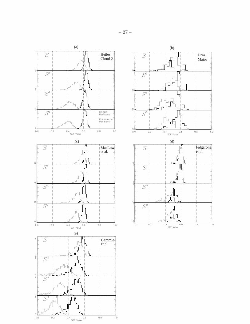
Fig. 3.— Figure 3 caption on next page
– 28 –
Figure 3–Histograms of SCF values for observed and simulated data cubes. To facilitate
comparison between the correlation functions, histograms have been normalized to the unit
interval for the unrandomized cube, and to an integral equal to the unrandomized cube
for the randomized cube. The histogram shown in heavy print represents the correlations
for the spectra in their original positions and the lighter line indicates the distribution
for randomized positions. Distributions are shown for: (a) observed C18O map of the
star-forming cloud Heiles Cloud 2 (deVries et al., 1998); (b) observed 12CO(2-1) map of
the Ursa Major unbound high-latitude cloud (Falgarone et al. 1994); (c) magnetic, non-
self-gravitating simulation of Mac Low et al. 1998; (d) non-magnetic, non-self-gravitating
simulation of Porter et al. (1994) cube used by Falgarone et al. (1994); and (e) magnetic,
self-gravitating simulation of Gammie et al. (1999). Table 2 lists the properties of the data
sets illustrated, and Table 3 compares the means and standard deviations of distributions
shown here. The four variants of the SCF are described in Table 1.
– 29 –
0.8
0.6
0.4
0.2
1.0
0.3
0.2
0.1
0.0
0.40.0
2 4 6 8 10 12 14 16
S
Sl
Ss
S0
Resolution [Pixels]
Sta
nd
ard
De
via
tion
of
SC
F D
istr
ibu
tion
Mea
n V
alue
of
SC
F
Randomized Positions
Original Positions
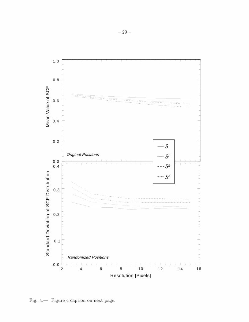
Fig. 4.— Figure 4 caption on next page.

– 30 –
Figure 4 – The behavior of the SCF as a function of changing resolution. For the HCl2
data set with uniform signal-to-noise (TA/σ)c = 5, the top panel shows the mean value of
the SCF as a function of the size of the box over which the SCF is calculated. The bottom
panel shows the 1 − σ width of the distribution of the SCF, for the same noise-equalized
HCl 2 data set, but with positions randomized. For any randomized cube, the mean of the
SCF is independent of resolution, and only the width of the distribution changes, as shown.
In creating these plots, runs using 3, 5, 7, 11, 13, and 15 pixel square sampling areas for the
SCF are used.