the spectrum of superconformal theories - physics and...
TRANSCRIPT
The Spectrum of Superconformal
Theories
A Dissertation Presented
by
Wenbin Yan
to
The Graduate School
in Partial Fulfillment of the Requirements
for the Degree of
Doctor of Philosophy
in
Physics and Astronomy
Stony Brook University
August 2012
Stony Brook University
The Graduate School
Wenbin Yan
We, the dissertation committee for the above candidate for theDoctor of Philosophy degree, hereby recommend
acceptance of this dissertation.
Leonardo Rastelli – Dissertation AdvisorProfessor, C.N. Yang Institute for Theoretical Physics
Peter van Nieuwenhuizen – Chairperson of DefenseProfessor, C.N. Yang Institute for Theoretical Physics
Robert McCarthyProfessor, Department of Physics and Astronomy
Martin RocekProfessor, C.N. Yang Institute for Theoretical Physics
Alexander KirillovProfessor, Department of Mathematics
Stony Brook University
This dissertation is accepted by the Graduate School
Charles TaberInterim Dean of the Graduate School
ii
Abstract of the Dissertation
The Spectrum of Superconformal Theories
by
Wenbin Yan
Doctor of Philosophy
in
Physics and Astronomy
Stony Brook University
2012
The spectrum is one of the basic information of any quantum fieldtheory. In general, it is difficult to obtain the full quantum spec-trum of QFT. However, in the case of four dimensional supercon-formal theories, certain information of the quantum spectrum canbe extracted exactly. In such theories one can compute exactlycertain observables containing spectral information with the helpof localization technique.
One such observable is the superconformal index, which is a par-tition function of the 4d theory on S3 × S1, twisted by variouschemical potentials. This index counts the states of the 4d theorybelonging to short multiplets, up to equivalent relations that setto to zero all sequences of short multiplets that may in principlerecombine into long ones. By construction, the index is invariantunder continuous deformations of the theory. The superconformalindex is studied for the class ofN = 2 4d superconformal field theo-ries introduced by Gaiotto. These theories are defined by compact-ifying the (2, 0) 6d theory on a Riemann surface with punctures.The index of the 4d theory associated to an n-punctured Riemann
iii
surface can be interpreted as the n-point correlation function ofa 2d topological QFT living on the surface, which can also be i-dentified as a certain deformation of two-dimensional Yang-Millstheory. With the help of different symmetric polynomials, even ex-plicit formulae are conjectured for all A-type quivers of such classof theories, which in general do not have Lagrangian description.Besides theN = 2 theories, the superconformal index of theN = 1Y p,q quiver gauge theories is also evaluated using Romeslberger’sprescription. For the conifold quiver Y 1,0 the result agrees exact-ly at large N with a previous calculation in the dual AdS5 × T 1,1
supergravity.
The superconformal index of a 4d gauge theory is computed bya matrix integral arising from localization of the supersymmetricpath integral on S3 × S1 to the saddle point. As the radius of thecircle goes to zero, it is natural to expect that the 4d path inte-gral becomes the partition function of dimensionally reduced gaugetheory on S3. We show that this is indeed the case and recover thematrix integral of Kapustin, Willett and Yaakov from the matrixintegral that computes the superconformal index. Remarkably, thesuperconformal index of the “parent” 4d theory can be thought ofas the q-deformation of the 3d partition function.
iv

To my parents and Luyi.
Contents
List of Figures ix
List of Tables xiii
Acknowledgements xvi
1 Introduction 1
2 Review of The Superconformal Index 62.1 The N = 2 Superconformal Index . . . . . . . . . . . . . . . . 72.2 The N = 1 Superconformal Index . . . . . . . . . . . . . . . . 10
2.2.1 Romelsberger’s prescription . . . . . . . . . . . . . . . 112.2.2 Computing the index . . . . . . . . . . . . . . . . . . . 12
2.3 A universal result about N = 2 → N = 1 flows . . . . . . . . 152.4 Elliptic Hypergeometric Expressions for the Index . . . . . . . 162.5 4d Index as a path integral on S3 × S1 . . . . . . . . . . . . . 19
3 S-duality and Two Dimensional Topological Field Theory 213.1 The Index in A1 Theories . . . . . . . . . . . . . . . . . . . . 23
3.1.1 2d TQFT from the Superconformal Index . . . . . . . 253.1.2 Associativity of the Algebra . . . . . . . . . . . . . . . 29
3.2 Argyres-Seiberg duality and the index of E6 SCFT . . . . . . 343.2.1 Weakly-coupled frame . . . . . . . . . . . . . . . . . . 353.2.2 Strongly-coupled frame and the index of E6 SCFT . . . 373.2.3 S-duality checks of the E6 index . . . . . . . . . . . . . 43
4 TQFT Structure of the Index for An-Type Quivers 494.1 Limits of the index with additional supersymmetry . . . . . . 524.2 Hall-Littlewood index . . . . . . . . . . . . . . . . . . . . . . . 56
4.2.1 SU(2) quivers . . . . . . . . . . . . . . . . . . . . . . . 564.2.2 Higher rank: preliminaries . . . . . . . . . . . . . . . . 59
vi
4.2.3 SU(3) quivers – the E6 SCFT . . . . . . . . . . . . . . 604.2.4 A conjecture for the structure constants with generic
punctures . . . . . . . . . . . . . . . . . . . . . . . . . 634.2.5 SU(4) quivers – T4 and the E7 SCFT . . . . . . . . . . 644.2.6 SU(6) quivers – the E8 SCFT . . . . . . . . . . . . . . 674.2.7 Large k limit . . . . . . . . . . . . . . . . . . . . . . . 69
4.3 Schur index . . . . . . . . . . . . . . . . . . . . . . . . . . . . 704.4 Macdonald index . . . . . . . . . . . . . . . . . . . . . . . . . 724.5 Coulomb-branch index . . . . . . . . . . . . . . . . . . . . . . 76
5 Reducing the 4d Index to the S3 Partition Function 805.1 4d Index to 3d Partition function on S3 . . . . . . . . . . . . . 81
5.1.1 Building blocks of the matrix models . . . . . . . . . . 815.2 4d↔ 3d dualities . . . . . . . . . . . . . . . . . . . . . . . . . 84
6 The Superconformal Index of N = 1 IR Fixed Points 866.1 The Y p,q quiver gauge theories . . . . . . . . . . . . . . . . . . 87
6.1.1 Toric Duality . . . . . . . . . . . . . . . . . . . . . . . 906.2 Large N evaluation of the index . . . . . . . . . . . . . . . . . 936.3 T 1,1 Index from Supergravity . . . . . . . . . . . . . . . . . . . 96
7 Discussion 99
A Duality 102A.1 The Representation Basis . . . . . . . . . . . . . . . . . . . . 102A.2 TQFT Algebra for v = t . . . . . . . . . . . . . . . . . . . . . 103A.3 t expansion in the weakly-coupled frame . . . . . . . . . . . . 107A.4 Inversion theorem . . . . . . . . . . . . . . . . . . . . . . . . . 108A.5 The Coulomb and Higgs branch operators of E6 SCFT . . . . 110A.6 Identities from S-duality . . . . . . . . . . . . . . . . . . . . . 111
B MacDonald 113B.1 Construction of the diagonal expression for the SU(2) HL index 113B.2 Index of short multiplets of N = 2 superconformal algebra . . 117B.3 Large k limit of the genus g HL index . . . . . . . . . . . . . . 122B.4 The unrefined HL index of T4 . . . . . . . . . . . . . . . . . . 123B.5 Proof of the SU(2) Schur index identity . . . . . . . . . . . . 124
C Refinement of 3d partition function 126
D N = 1 superconformal shortening conditions and the index 129
vii

Bibliography 135
viii
List of Figures
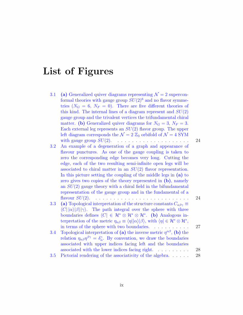
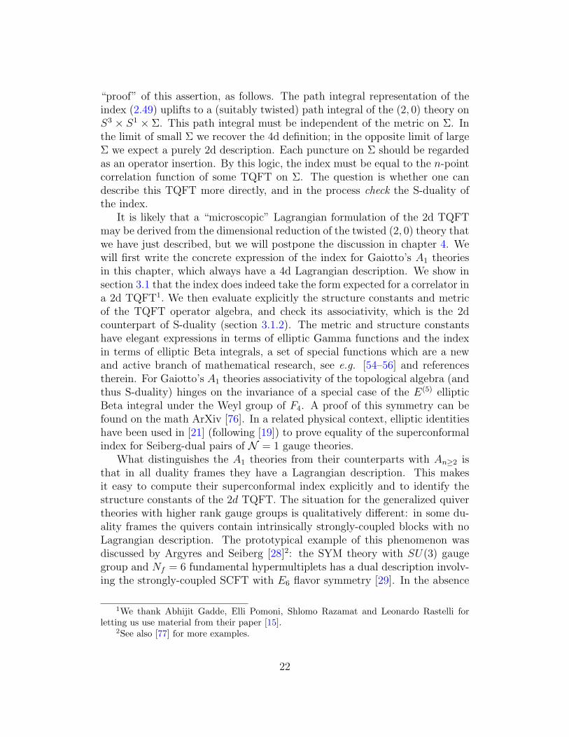
3.1 (a) Generalized quiver diagrams representing N = 2 supercon-formal theories with gauge group SU(2)6 and no flavor symme-tries (NG = 6, NF = 0). There are five different theories ofthis kind. The internal lines of a diagram represent and SU(2)gauge group and the trivalent vertices the trifundamental chiralmatter. (b) Generalized quiver diagrams for NG = 3, NF = 3.Each external leg represents an SU(2) flavor group. The upperleft diagram corresponds the N = 2 Z3 orbifold of N = 4 SYMwith gauge group SU(2). . . . . . . . . . . . . . . . . . . . . 24
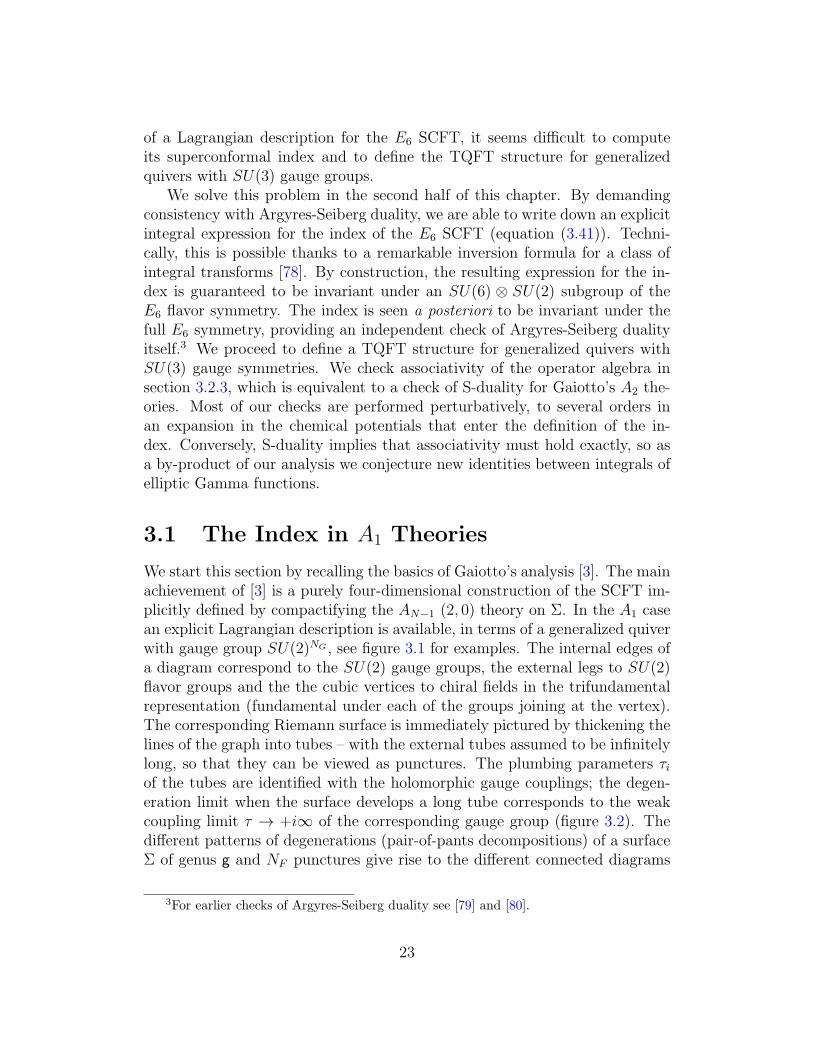
3.2 An example of a degeneration of a graph and appearance offlavour punctures. As one of the gauge coupling is taken tozero the corresponding edge becomes very long. Cutting theedge, each of the two resulting semi-infinite open legs will beassociated to chiral matter in an SU(2) flavor representation.In this picture setting the coupling of the middle legs in (a) tozero gives two copies of the theory represented in (b), namelyan SU(2) gauge theory with a chiral field in the bifundamentalrepresentation of the gauge group and in the fundamental of aflavour SU(2). . . . . . . . . . . . . . . . . . . . . . . . . . . 24
3.3 (a) Topological interpretation of the structure constants Cαβγ ≡⟨C| |α⟩|β⟩|γ⟩. The path integral over the sphere with threeboundaries defines ⟨C| ∈ H∗ ⊗ H∗ ⊗ H∗. (b) Analogous in-terpretation of the metric ηαβ ≡ ⟨η||α⟩|β⟩, with ⟨η| ∈ H∗ ⊗H∗,in terms of the sphere with two boundaries. . . . . . . . . . . 27
3.4 Topological interpretation of (a) the inverse metric ηαβ, (b) therelation ηαβη
βγ = δγα. By convention, we draw the boundariesassociated with upper indices facing left and the boundariesassociated with the lower indices facing right. . . . . . . . . . 28
3.5 Pictorial rendering of the associativity of the algebra. . . . . . 28
ix
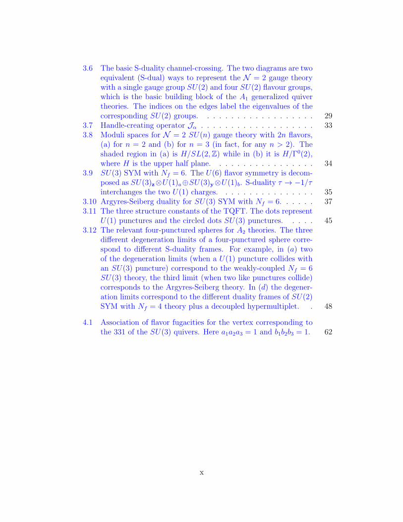
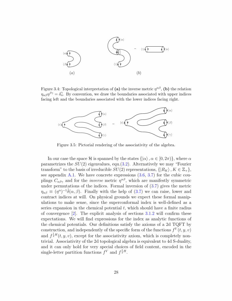
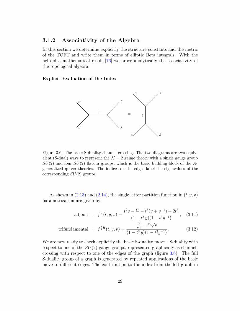
3.6 The basic S-duality channel-crossing. The two diagrams are twoequivalent (S-dual) ways to represent the N = 2 gauge theorywith a single gauge group SU(2) and four SU(2) flavour groups,which is the basic building block of the A1 generalized quivertheories. The indices on the edges label the eigenvalues of thecorresponding SU(2) groups. . . . . . . . . . . . . . . . . . . 29
3.7 Handle-creating operator Jα . . . . . . . . . . . . . . . . . . . 333.8 Moduli spaces for N = 2 SU(n) gauge theory with 2n flavors,
(a) for n = 2 and (b) for n = 3 (in fact, for any n > 2). Theshaded region in (a) is H/SL(2,Z) while in (b) it is H/Γ0(2),where H is the upper half plane. . . . . . . . . . . . . . . . . 34
3.9 SU(3) SYM with Nf = 6. The U(6) flavor symmetry is decom-posed as SU(3)z⊗U(1)a⊕SU(3)y⊗U(1)b. S-duality τ → −1/τinterchanges the two U(1) charges. . . . . . . . . . . . . . . . 35
3.10 Argyres-Seiberg duality for SU(3) SYM with Nf = 6. . . . . . 373.11 The three structure constants of the TQFT. The dots represent
U(1) punctures and the circled dots SU(3) punctures. . . . . 453.12 The relevant four-punctured spheres for A2 theories. The three
different degeneration limits of a four-punctured sphere corre-spond to different S-duality frames. For example, in (a) twoof the degeneration limits (when a U(1) puncture collides withan SU(3) puncture) correspond to the weakly-coupled Nf = 6SU(3) theory, the third limit (when two like punctures collide)corresponds to the Argyres-Seiberg theory. In (d) the degener-ation limits correspond to the different duality frames of SU(2)SYM with Nf = 4 theory plus a decoupled hypermultiplet. . 48
4.1 Association of flavor fugacities for the vertex corresponding tothe 331 of the SU(3) quivers. Here a1a2a3 = 1 and b1b2b3 = 1. 62
x
4.2 Association of the flavor fugacities for a generic puncture. Punc-tures are classified by embeddings of SU(2) in SU(k), so theyare specified by the decomposition of the fundamental repre-sentation of SU(k) into irreps of SU(2), that is, by a partitionof k. Graphically we represent the partition by an auxiliaryYoung diagram Λ with k boxes, read from left to right. Inthe figure we have the fundamental of SU(26) decomposed as5+5+4+4+4+2+1+1. The commutant of the embeddinggives the residual flavor symmetry, in this case S(U(3)×U(2)×U(2)×U(1)), where the S(. . . ) constraint amounts to removingthe overall U(1). The τ variable is viewed here as an SU(2)fugacity, while the Latin variables are fugacities of the residualflavor symmetry. The S(. . . ) constraint implies that the flavorfugacities satisfy (ab)5(cde)4f 2gh = 1. . . . . . . . . . . . . . . 63
4.3 The factors aik associated to a generic Young diagram. Theupper index is the row index and the lower is the column index.In aik one takes the inverse of flavor fugacities while τ is treatedas real number. As before, the flavor fugacities in this examplesatisfy (ab)5(cde)4f 2gh = 1. . . . . . . . . . . . . . . . . . . . 65
4.4 Association of the flavor fugacities for the E7 vertex. Here∏4i=1 bi =
∏4i=1 ai = 1. . . . . . . . . . . . . . . . . . . . . . . 66
4.5 Association of the flavor fugacities for the E8 vertex. Here∏3i=1 bi =
∏6i=1 ai = 1. . . . . . . . . . . . . . . . . . . . . . . 68
4.6 The bottom left box is assigned 0. The assigned integer increas-es from left to right. As we move up, the first box of each rowis assigned the same number as the last box in the row below. 78
6.1 Left: quiver diagram for Y 4,4. Right: quiver diagram for Y 4,0. 886.2 Quiver diagram for Y 1,0 (the conifold theory T 1,1). The solid
(cyan) arrow represents the U field, the dash-dot (blue) arrowrepresents the Y field and the dashed (green) arrow representsthe Z field. . . . . . . . . . . . . . . . . . . . . . . . . . . . . 89
6.3 Quiver of Y 1,1 theory. Solid (cyan) arrow represents U field,dash-dot-dot arrow (red) represents V field and dash-dot arrow(blue) represents Y field. . . . . . . . . . . . . . . . . . . . . . 89
6.4 Quiver diagram for Y 4,2, obtained from Y 4,4 by using the pro-cedure in [1]. . . . . . . . . . . . . . . . . . . . . . . . . . . . 90
6.5 A different quiver diagram for Y 4,2, related to the diagram aboveby toric duality. . . . . . . . . . . . . . . . . . . . . . . . . . . 90
xi
6.6 Left: initial quiver. The node represents a SU(N) gauge group.The effective number of flavors is Nf = 2N . Middle: quiverafter Seiberg duality. The node represents the Seiberg dualgauge group SU(2N − N) = SU(N). All arrows are reversedand mesons (with appropriate R-charges) are added. Right: thedash-dot-dot (red) and dot (orange) mesons cancel each otherout by equ.(4.15). This can be understood physically in termsof integrating out massive degrees of freedom [31]. . . . . . . . 92
6.7 Left: Y 4,2 quiver in figure 6.4. Middle: Seiberg dual on node 1.Right: the quiver in figure 6.5 is obtained by swap node 1 and2 in the middle figure. . . . . . . . . . . . . . . . . . . . . . . 92
A.1 Constructing the metric by capping off the trivalent vertex. . . 105A.2 Topological interpretation of the property ηce ηea = δca. . . . . . 106A.3 The consistency requirement δzc Cabz = Cabc. . . . . . . . . . . 106A.4 The sphere (a) and the torus (b) partition functions. . . . . 107A.5 The integration contour Cw (green). The dashed (black) circle
is the unit circle T. Black dots are poles of Γ(√
vt2w±1 z±1
).
There are four sequences of poles: two sequences starting at√v
t2w±1 and converging to z = 0, and two sequences starting at
t2√vw±1 and converging to z = ∞. The contour encloses the two
former sequences. . . . . . . . . . . . . . . . . . . . . . . . . 109
xii
List of Tables
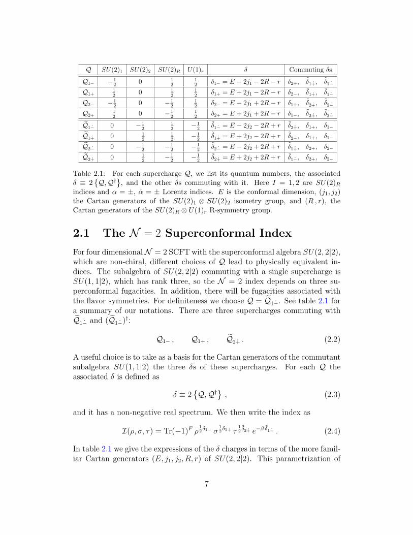
2.1 For each supercharge Q, we list its quantum numbers, the asso-ciated δ ≡ 2
Q,Q†, and the other δs commuting with it. Here
I = 1, 2 are SU(2)R indices and α = ±, α = ± Lorentz indices.E is the conformal dimension, (j1, j2) the Cartan generators ofthe SU(2)1 ⊗ SU(2)2 isometry group, and (R , r), the Cartangenerators of the SU(2)R ⊗ U(1)r R-symmetry group. . . . . 7
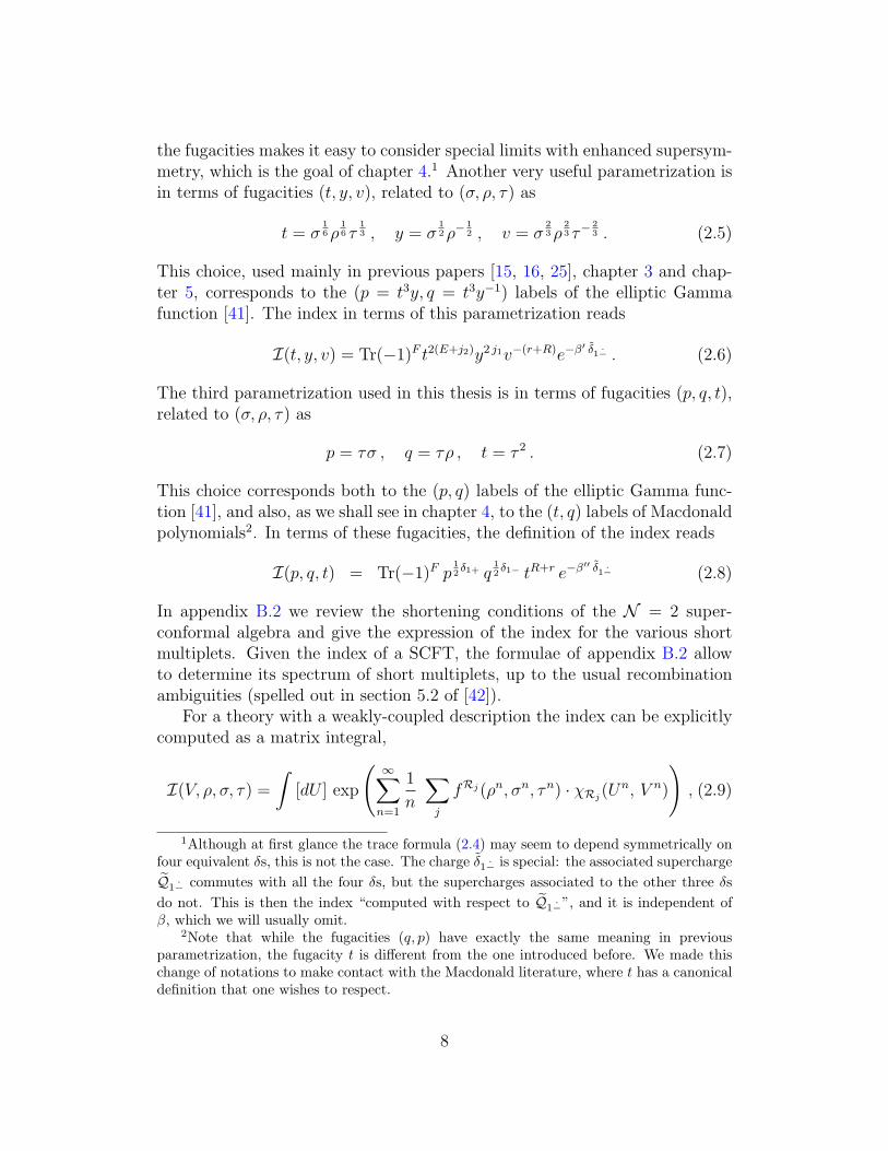
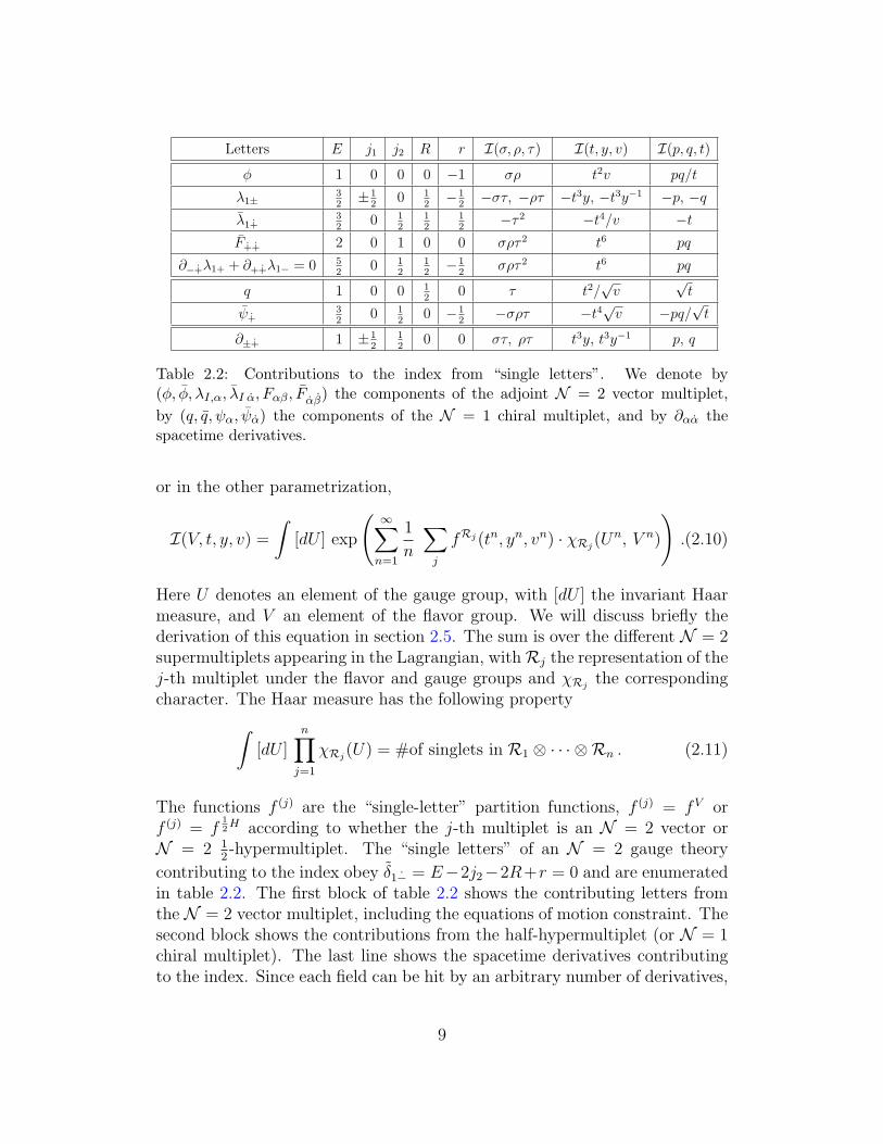
2.2 Contributions to the index from “single letters”. We denote by(ϕ, ϕ, λI,α, λI α, Fαβ, Fαβ) the components of the adjoint N = 2
vector multiplet, by (q, q, ψα, ψα) the components of the N = 1chiral multiplet, and by ∂αα the spacetime derivatives. . . . . 9
2.3 The “letters” of an N = 1 chiral multiplet and their contri-butions to the index. Here δL = E − 2j1 +
32rUV and δRUV =
E − 2j2 − 32rUV . A priori we have to take into account the
free equations of motion ∂ψ = 0 and ϕ = 0, which implyconstraints on the possible words, but we see that in this caseequations of motions have δUV = 0 so they do not change the in-dex. Finally there are two spacetime derivatives contributing tothe index, and their multiple action on the fields is responsiblefor the denominator of the index, 1/(1− t3y±1) =
∑∞n=0(t
3y±1)n. 13
3.1 The structure constants and the metric in terms of elliptic Gam-ma functions. For brevity we have left implicit the parametersof the Gamma functions, p = t3y and q = t3y−1. We have de-fined a ≡ exp(iα), b ≡ exp(iβ), and c ≡ exp(iγ). Recall alsoκ ≡ (p; p)(q; q)/4πi and ∆(α) ≡ (sin2 α)/π. . . . . . . . . . . 32
4.1 The structure constants, the cap, and the metric for the TQFTof the Macdonald index. . . . . . . . . . . . . . . . . . . . . . 75
xiii
6.1 Short multiplets appearing in the KK reduction of Type IIBsupergravity on AdS5 × T 1,1. In the last column, we sum-marize the full index contributions of multiplets by listing theSU(2)s×SU(2)l characters multiplying IL
[r, 12]L+for first four rows
and IL[r,0]L+
for remaining rows. The range of r is specified by
the two conditions that r ≥ −1 and that the SU(2)s × SU(2)lrepresentation makes sense. The chemical potentials a and bcouple to SU(2)s × SU(2)l flavor charges respectively. Excep-tion: The first row of GravitinoI starts from r = 0. The r = −1state of GravitinoI gives rise to the Dirac multiplet D(0, 1
2) due
to additional shortening. It corresponds in the dual field theoryto a decoupled U(1) vector multiplet. . . . . . . . . . . . . . 97
A.1 The basic building blocks of the topological algebra in the v = tcase. . . . . . . . . . . . . . . . . . . . . . . . . . . . . . . . . 105
B.1 Shortening conditions and short multiplets for the N = 2 su-perconformal algebra. . . . . . . . . . . . . . . . . . . . . . . . 118
B.2 The coefficients of P86(τ). The coefficient of τ 86−k is equal tothe coefficient of τ k . . . . . . . . . . . . . . . . . . . . . . . . 123
D.1 Possible shortening conditions for the N = 1 superconformalalgebra. . . . . . . . . . . . . . . . . . . . . . . . . . . . . . . 129
D.2 A long multiplet ofN = 1 superconformal algebra. The SU(2, 2)multiplets that are boxed form a short Br(0,j2) multiplet forj1 = 0,∆ = −3
2r. The left-handed B can be obtained by reflect-
ing the table (that is, sending r → −r and j1 ↔ j2). In general,when j1(j2) = 0, the SU(2, 2) multiplets (j1− 1
2, any)((any, j2−
12)) are set to zero, resulting in further shortening. . . . . . . . 131
D.3 A long multiplet ofN = 1 superconformal algebra. The SU(2, 2)multiplets that are boxed form a semi-short Cr(j1,j2) multiplet for∆ = 2+2j1− 3
2r. The left-handed C can be obtained by reflect-
ing the table (that is, sending r → −r and j1 ↔ j2). In general,when j1(j2) = 0, the SU(2, 2) multiplets (j1− 1
2, any)((any, j2−
12)) are set to zero, resulting in further shortening. . . . . . . . 131
D.4 Multiplet structure of C(j1,j2). The shortening conditions are∆ = 2 + j1 + j2 and 3
2r = (j1 − j2). . . . . . . . . . . . . . . . 132
xiv
D.5 Multiplet structure of D(0,j2). The shortening conditions are∆ = 1 + j2 = −3
2r and j1 = 0. The multiplet D(j1,0) could be
obtained by j1 ↔ j2, r ↔ −r or by simply reflecting the table.The shortening conditions in that case are ∆ = 1+ j1 =
32r and
j2 = 0. . . . . . . . . . . . . . . . . . . . . . . . . . . . . . . 132D.6 Indices IL and IR of the various short and semi-short multiplets. 134
xv
Acknowledgements
First and foremost, it is with immense gratitude that I acknowledge the sup-port and help of my advisor Prof. Leonardo Rastelli. My doctoral endeavorwould not have been possible without his constant help and guidance. It hasbeen an edifying experience which I cherish forever to work with Prof. Leonar-do Rastelli. While guiding me at every step, he taught me the courage to beindependent. Conceptual clarity, creative imagination and physical intuitionconstitute the fountain-head of worthwhile research. I learned this fundamen-tal rule of scientific craftsmanship with the help of my advisor. My relationwith him has been and remains forever very special.
It gives me great pleasure in acknowledging Prof. Peter van Nieuwen-huizen, a doyen and a luminary among the theoretical physicists. As soon as Ijoined the department as a graduate student, he extended me the privilege ofinteracting with him. I had the fortune of learning from his advanced cours-es on almost every major subject of modern theoretical physics which formthe foundation on which my current understanding the subject rests. He hasbeen a source of inspiration and encouragement. I owe a great deal to him inrelation to the intricate texture of the matrix of the discipline within whichI worked. I consider it an honor to work with Prof. Sally Dawson on sometopics of particle phenomenology which link me back from ten dimensions toreality. I am obliged to Prof. Martin Rocek interaction with whom has beenacademically highly rewarding and personally very gratifying. I am beholdento all my teachers at Stony Brook whose pedagogical excellence ensured that Iinternalized the lexicon and the grammar of Fundamental Physics. I appreci-ate deeply all the help rendered by the office staff both at the Yang Institute ofTheoretical Physics and Department of Physics and Astronomy, Stony BrookUniversity.
I would also like to place on record my deep appreciation for the valuableco-operation and enormous goodwill shown by my collaborators in research.I must specially mention here Abhijit Gadde, Shlomo Razamat and PedroLiendo. I enjoyed every bit of my interaction with them. My interaction withmy friends in the department and outside has been extremely refreshing. To
grow with them and helping each other in growing is a memorable experiencein a lifetime. I fondly mention the names of Dharmesh, Marcos, Ozan, Prerit,Sujan, Xiaojie, Xiaoyang and others.
Throughout my stay at Stony Brook, I have enjoyed the emotional supportprovided by my parents back home in China and my girlfriend Luyi at Berkeley.I would not have made it this far without their full-hearted support
Finally, I am highly indebted to the Stony Brook University, especially theYang Institute of Theoretical Physics and Simons Center for Geometry andPhysics for providing all facilities for research, congenial ambience and excitingenvironment.
Chapter 1
Introduction
The spectrum is always the fundamental information one wants to understandfirst when studying any quantum theory, of which the most classic examplemight be Bohr’s computation of hydrogen levels. Nevertheless, it is alwaysdifficult to obtain the exact spectrum of quantum theories beyond certainsimplest cases. For a long time, perturbation theory is the only way to tacklethis kind of problems. Although bosonic symmetries can simplify the study ofany dynamical system, they are still not constraining enough to prevent quan-tum corrections from rapidly becoming intractable with increasing loop order.However, supersymmetry is able to help keep the quantum corrections undercontrol, thus becomes a powerful tool for extracting exact information aboutquantum field theories. In recent years, using methods based on localization,several exact quantities in supersymmetric gauge theories have been comput-ed. This thesis is devoted to one of such observables - the superconformalindex.
Superconformal algebras that have R-charges on the right hand side con-tain special BPS multiplets, which occur only at certain values of energiesor conformal dimensions fixed by their charges and have few states than thegeneric multiplets. An infinitesimal change in the energy (or conformal dimen-sion) of a BPS multiplet turns it into a generic multiplet with finite increaseof the number of states. Thus the BPS states are guaranteed to be protectedexcluding the ones which may combine into a generic representation. The su-perconformal index [2] is constructed to receive contributions only from thoseprotected states of a superconformal field theory (SCFT). It is a weightedsum over the states of the theory, which by construction evaluates to zero ona generic (long) multiplet. It follows that the index is invariant under ex-actly marginal deformations, since it is not affected by the recombinations ofshort multiplets into long ones (or viceversa) that may occur as parametersare varied. For SCFTs admitting a weakly-coupled limit, the index can then
1
be evaluated exactly in free-field theory by a straightforward counting proce-dure, and takes the form of a matrix integral. However, the superconformalindex does not limit itself into SCFTs admitting a weakly-coupled limit only.Some strongly coupled SCFTs may be related to other weakly coupled onesby dualities, thus the indices of the former can be computed by the indicesof the later. With the help of suitable dualities and mathematical identities,we can even obtain the superconformal indices of theories without Lagrangiandescription. The results definitely improve our knowledge on the (protected)spectrum of such theories.
For example, there is a very general web of duality connections relatingN = 2 4d superconformal field theories, the vast majority of which do nothave a weakly-coupled regime nor a conventional Lagrangian description. Thisfact, which may have been suspected since the early days of string dualities,has taken center stage after the more explicit construction of the N = 2superconformal theories of “class S” [3, 4], most of which are not Lagrangian.1
Class S theories arise by compactification of the six-dimensional (2, 0) theoryon a punctured Riemann surface C. There is a growing dictionary relatingfour-dimensional quantities with quantities associated to the surface C. Abasic entry of the dictionary identifies the exactly marginal couplings of the4d theory with the complex structure moduli of C.2 According to the celebratedAGT conjecture [9–11], the 4d partition functions on the Ω-background [12]and on S4 [13] are computed by Liouville/Toda theory on C. An analogousrelation exists between the 4d superconformal index [2, 14] (which can alsobe viewed as a supersymmetric partition function on S3×S1) and topologicalquantum field theory (TQFT) on C [15–18]. This last relation is a main topicof this thesis.
The superconformal index is a simpler observable than the S4 partitionfunction, and it should be a good starting point for a microscopic derivation ofthe 4d/2d dictionary from the 6d (2,0) theory. Being coupling-independent, theindex is computed by a topological correlator on C [15], as opposed to a CFTcorrelator as in the AGT correspondence. For the subset of class S theoriesthat have a Lagrangian description, it can be easily evaluated in the free-fieldlimit, unlike the S4 partition function, which is sensitive to non-perturbativephysics and requires a sophisticated localization calculation [12, 13].
Despite these simplifying features, the index of class S theories is still a
1Though very large, class S does not cover the full space of N = 2 SCFTs. Counterex-amples can be found e.g. in [3, 5]. See [5–7] for the beginning of a classification programfor N = 2 4d SCFTs.
2On the other hand, the conformal factor of the metric on C is irrelevant (in the RGsense) and its memory lost in the IR SCFT. See [8] for a recent holographic check of thisfact.
2
very non-trivial observable with remarkable mathematical structure. First ofall, there is no direct way to compute it for the non-Lagrangian SCFTs, whichby definition are not continuously connected to free-field theories.3 An indirectroute is to use the generalized S-dualities [3, 28] that relate non-Lagrangianwith Lagrangian theories. This is the strategy used in [16] to evaluate the indexof the strongly-coupled SCFT with E6 flavor symmetry [29]. In principle thisprocedure could be carried out recursively to find the index of all the non-Lagrangian theories, but it suffers from two drawbacks: conceptually, onewould rather use the index to test dualities, than assume dualities to computethe index; and practically, this program gets quickly too complicated to beuseful.
What one should aim for is a direct algorithm that applies to all class Stheories – one would like to identify and solve the 2d TQFT that computesthe index. The first step in this direction has been recently taken in [17]: in alimit where a single superconformal fugacity is kept (out of the original three)the 2d topological theory is recognized as the zero-area limit of q-deformedYang-Mills theory. In [18] we generalize this result to a two-parameter slice(q, t) of the three-dimensional fugacity space, which reduces to the limit con-sidered in [17] for t = q. We give a fully explicit prescription to computethis limit of the index for the most general4 A-type generalized quiver of classS. The principle that selects this particular fugacity slice is supersymme-try enhancement, which leads to simplifications. We study systematically thelimits where the index receives contributions only from states annihilated bymore than one supercharge. The (q, t) slice is the most general limit of thiskind sensitive to the flavor fugacities associated to the punctures. We alsostudy another interesting slice (Q, T ), where the index receives contributiononly from “Coulomb-branch” operators, which are flavor-neutral, so the flavordependence is lost.
On the other hand, some of the most important examples of interacting4d SCFTs do not have a (known) weakly-coupled description in any duali-ty frame. A large class are the N = 1 SCFTs that arise as IR fixed pointsof renormalization group flows, whose UV starting points are weakly-coupledtheories. A prescription to evaluate the index of such SCFTs was formulatedby Romelsberger [14, 19]. This prescription has so far been checked indirectly,
3We should mention that for N = 1 SCFTs obtained as IR points of an RG flow, aprescription to compute the index in terms of the UV field content and the charges of theanomaly free R-symmetry was put forward by Romelsberger [14, 19] and recently revisitedwith more rigor in [20]. Following the seminal work of Dolan and Osborn [21] there havebeen many checks and implications of this conjecture, see e.g. [22–27].
4In particular in [17] certain overall normalization factors were determined only for the-ories with special types of punctures. Here we fill this gap and work in complete generality.
3
by showing in several examples that it gives the same result for different RGflows that end in the same IR fixed point (i.e. the UV theories are Seibergdual). This was originally observed by Romelsberger, who performed a fewperturbative checks in a chemical potential expansion [14, 19]. Invariance ofthe N = 1 index under Seiberg duality was systematically demonstrated byDolan and Osborn [21], in a remarkable paper that first applied the elliptic hy-pergeometric machinery to the evaluation of the superconformal index. Theseresults were extended and generalized in [22–24, 26].
In [25] we apply Romelsberger’s prescription to a class of N = 1 SCFTsthat admit AdS duals. The canonical example is the conifold theory of Kle-banov and Witten [30]. There are infinitely many generalizations: the familiesof toric quivers Y p,q [1] and Lp,q,r [31]. We focus on Y p,q. In all these examplesthere is in principle an independent way to determine the index (at large N)from the dual supergravity. We explicitly show agreement between the gravitycalculation of Nakayama [32] and our field theory calculation for the case ofthe conifold quiver Y 1,0. According to taste, this can be viewed either as acheck of Romelsberger’s prescription, or as yet another check of AdS/CFT.The upshot is a sharper bulk/boundary dictionary.
As the superconformal index is successfully applied to both N = ∈ andN = ∞ theories, the partition function of supersymmetric gauge theories on S3
has been used to check a variety of 3d dualities including mirror symmetry [33]and Seiberg-like dualities [34]. Remarkably, the exact partition function hasalso allowed for a direct field theory computation of N3/2 degrees of freedomof ABJM theory [35, 36]. The S3 partition function of N = 2 theories isextremized by the exact superconformal R-symmetry [37–39] so just like thea-maximization in 4d, the 3d partition function can be used to determine theexact R-charges at interacting fixed points.
The superconformal index of a 4d gauge theory can be computed as a pathintegral on S3 × S1 with supersymmetric boundary conditions along S1. Allthe modes on the S1 contribute to this path integral. In a limit with theradius of the circle shrinking to zero the higher modes become very heavy anddecouple. The index is then given by a path integral over just the constantmodes on the circle. In other words, the superconformal index of the 4d theoryreduces to a partition function of the dimensionally reduced 3d gauge theoryon S3. The 3d theory preserves all the supersymmetries of the “parent” 4dtheory on S3 × S1. More generally, for any d dimensional manifold Md, onewould expect the index of a supersymmetric theory on Md × S1 to reduce tothe exact partition function of dimensionally reduced theory onMd. This ideawas applied by Nekrasov to obtain the partition function of 4d gauge theoryon Ω-deformed background as a limit of the index of a 5d gauge theory [12].
4
A crucial property of the four dimensional index that facilitates its compu-tation is the fact that it can be computed exactly by a saddle point integral.In the limit of vanishing circle radius, this matrix integral reduces to the onethat computes the partition function of 3d gauge theories on S3 [33, 40]. Itdoesn’t come as a surprise as the path integral of the N = 2 supersymmetricgauge theory on S3 was also shown to localize on saddle points of the action.
The rest of the thesis is organized as follows: in chapter 2 we review thedefinition of the superconformal index, the computation of the index in weaklycoupled SCFTs and the re-expression of the index by the special function calledthe elliptic gamma function. Chapter 3 and 4 deal with the application of theindex in N = ∈ class S theories and 2d topological field theory structurebehind. The reduction of the 4d index into a 3d partition function will bediscussed in chapter 5. Chapter 6 focuses mainly on the index of Y p,q quivergauge theories and a preliminary holographic check.
5
Chapter 2
Review of The SuperconformalIndex
The superconformal index [2] encodes the information about the protectedspectrum (which means its conformal dimension does not get quantum cor-rections) of a superconformal field theory (SCFT) that can be obtained fromrepresentation theory alone. The index of a 4d SCFT is defined as the Wit-ten index of the theory in radial quantization. Let Q be one of the Poincaresupercharges in the superconformal algebra of the theory, and Q† = S theconjugate conformal supercharge. Schematically, the index with respect to Qis defined as [2, 14, 19]
I(µi) = Tr (−1)F e−β δ e−µiMi , δ = 2Q,Q† , (2.1)
where the trace is over the Hilbert space of the theory on S3 (or Sd−1 in gen-eral d dimensions) in the usual radial quantization, F is the Fermion numberoperator, Mi are Q-closed conserved charges and µi the associated chemicalpotentials. Since states with δ > 0 come in boson/fermion pairs, only the δ = 0states contribute (the “harmonic representatives” of the cohomology classes ofQ), and the index is independent of β. There are infinitely many states withδ = 0 – this is true even for a single short irreducible representation of thesuperconformal algebra, because some of the non-compact generators (someof the spacetime derivatives) have δ = 0. The introduction of the chemicalpotentials µi serves both to regulate this divergence and to achieve a morerefined counting. From the index one can reconstruct the spectrum of shortmultiplets, up to the equivalence relations that set to zero the combinationsof short multiplets that may a priori recombine into long ones [2].
6
Q SU(2)1 SU(2)2 SU(2)R U(1)r δ Commuting δs
Q1− −12
0 12
12
δ1− = E − 2j1 − 2R− r δ2+, δ1+, δ1−
Q1+12
0 12
12
δ1+ = E + 2j1 − 2R− r δ2−, δ1+, δ1−
Q2− −12
0 −12
12
δ2− = E − 2j1 + 2R− r δ1+, δ2+, δ2−
Q2+12
0 −12
12
δ2+ = E + 2j1 + 2R− r δ1−, δ2+, δ2−
Q1− 0 −12
12
−12
δ1− = E − 2j2 − 2R + r δ2+, δ1+, δ1−
Q1+ 0 12
12
−12
δ1+ = E + 2j2 − 2R + r δ2−, δ1+, δ1−
Q2− 0 −12
−12
−12
δ2− = E − 2j2 + 2R + r δ1+, δ2+, δ2−
Q2+ 0 12
−12
−12
δ2+ = E + 2j2 + 2R + r δ1−, δ2+, δ2−
Table 2.1: For each supercharge Q, we list its quantum numbers, the associatedδ ≡ 2
Q,Q†, and the other δs commuting with it. Here I = 1, 2 are SU(2)R
indices and α = ±, α = ± Lorentz indices. E is the conformal dimension, (j1, j2)the Cartan generators of the SU(2)1 ⊗ SU(2)2 isometry group, and (R , r), theCartan generators of the SU(2)R ⊗ U(1)r R-symmetry group.
2.1 The N = 2 Superconformal Index
For four dimensionalN = 2 SCFT with the superconformal algebra SU(2, 2|2),which are non-chiral, different choices of Q lead to physically equivalent in-dices. The subalgebra of SU(2, 2|2) commuting with a single supercharge isSU(1, 1|2), which has rank three, so the N = 2 index depends on three su-perconformal fugacities. In addition, there will be fugacities associated withthe flavor symmetries. For definiteness we choose Q = Q1−. See table 2.1 fora summary of our notations. There are three supercharges commuting withQ1− and (Q1−)
†:
Q1− , Q1+ , Q2+ . (2.2)
A useful choice is to take as a basis for the Cartan generators of the commutantsubalgebra SU(1, 1|2) the three δs of these supercharges. For each Q theassociated δ is defined as
δ ≡ 2Q,Q† , (2.3)
and it has a non-negative real spectrum. We then write the index as
I(ρ, σ, τ) = Tr(−1)F ρ12δ1− σ
12δ1+ τ
12δ2+ e−β δ1− . (2.4)
In table 2.1 we give the expressions of the δ charges in terms of the more famil-iar Cartan generators (E, j1, j2, R, r) of SU(2, 2|2). This parametrization of
7
the fugacities makes it easy to consider special limits with enhanced supersym-metry, which is the goal of chapter 4.1 Another very useful parametrization isin terms of fugacities (t, y, v), related to (σ, ρ, τ) as
t = σ16ρ
16 τ
13 , y = σ
12ρ−
12 , v = σ
23ρ
23 τ−
23 . (2.5)
This choice, used mainly in previous papers [15, 16, 25], chapter 3 and chap-ter 5, corresponds to the (p = t3y, q = t3y−1) labels of the elliptic Gammafunction [41]. The index in terms of this parametrization reads
I(t, y, v) = Tr(−1)F t2(E+j2)y2 j1v−(r+R)e−β′ δ1− . (2.6)
The third parametrization used in this thesis is in terms of fugacities (p, q, t),related to (σ, ρ, τ) as
p = τσ , q = τρ , t = τ 2 . (2.7)
This choice corresponds both to the (p, q) labels of the elliptic Gamma func-tion [41], and also, as we shall see in chapter 4, to the (t, q) labels of Macdonaldpolynomials2. In terms of these fugacities, the definition of the index reads
I(p, q, t) = Tr(−1)F p12δ1+ q
12δ1− tR+r e−β′′ δ1− (2.8)
In appendix B.2 we review the shortening conditions of the N = 2 super-conformal algebra and give the expression of the index for the various shortmultiplets. Given the index of a SCFT, the formulae of appendix B.2 allowto determine its spectrum of short multiplets, up to the usual recombinationambiguities (spelled out in section 5.2 of [42]).
For a theory with a weakly-coupled description the index can be explicitlycomputed as a matrix integral,
I(V, ρ, σ, τ) =∫
[dU ] exp
(∞∑n=1
1
n
∑j
fRj(ρn, σn, τn) · χRj(Un, V n)
), (2.9)
1Although at first glance the trace formula (2.4) may seem to depend symmetrically onfour equivalent δs, this is not the case. The charge δ1− is special: the associated supercharge
Q1− commutes with all the four δs, but the supercharges associated to the other three δs
do not. This is then the index “computed with respect to Q1−”, and it is independent ofβ, which we will usually omit.
2Note that while the fugacities (q, p) have exactly the same meaning in previousparametrization, the fugacity t is different from the one introduced before. We made thischange of notations to make contact with the Macdonald literature, where t has a canonicaldefinition that one wishes to respect.
8
Letters E j1 j2 R r I(σ, ρ, τ) I(t, y, v) I(p, q, t)
ϕ 1 0 0 0 −1 σρ t2v pq/t
λ1±32
±12
0 12
−12
−στ, −ρτ −t3y, −t3y−1 −p, −qλ1+
32
0 12
12
12
−τ 2 −t4/v −tF++ 2 0 1 0 0 σρτ 2 t6 pq
∂−+λ1+ + ∂++λ1− = 0 52
0 12
12
−12
σρτ 2 t6 pq
q 1 0 0 12
0 τ t2/√v
√t
ψ+32
0 12
0 −12
−σρτ −t4√v −pq/
√t
∂±+ 1 ±12
12
0 0 στ, ρτ t3y, t3y−1 p, q
Table 2.2: Contributions to the index from “single letters”. We denote by(ϕ, ϕ, λI,α, λI α, Fαβ , Fαβ) the components of the adjoint N = 2 vector multiplet,
by (q, q, ψα, ψα) the components of the N = 1 chiral multiplet, and by ∂αα thespacetime derivatives.
or in the other parametrization,
I(V, t, y, v) =∫
[dU ] exp
(∞∑n=1
1
n
∑j
fRj(tn, yn, vn) · χRj(Un, V n)
).(2.10)
Here U denotes an element of the gauge group, with [dU ] the invariant Haarmeasure, and V an element of the flavor group. We will discuss briefly thederivation of this equation in section 2.5. The sum is over the different N = 2supermultiplets appearing in the Lagrangian, withRj the representation of thej-th multiplet under the flavor and gauge groups and χRj
the correspondingcharacter. The Haar measure has the following property∫
[dU ]n∏
j=1
χRj(U) = #of singlets in R1 ⊗ · · · ⊗ Rn . (2.11)
The functions f (j) are the “single-letter” partition functions, f (j) = fV orf (j) = f
12H according to whether the j-th multiplet is an N = 2 vector or
N = 2 12-hypermultiplet. The “single letters” of an N = 2 gauge theory
contributing to the index obey δ1− = E−2j2−2R+r = 0 and are enumeratedin table 2.2. The first block of table 2.2 shows the contributing letters fromthe N = 2 vector multiplet, including the equations of motion constraint. Thesecond block shows the contributions from the half-hypermultiplet (or N = 1chiral multiplet). The last line shows the spacetime derivatives contributingto the index. Since each field can be hit by an arbitrary number of derivatives,
9
the derivatives give a multiplicative contribution to the single-letter partitionfunctions of the form
∞∑m=0
∞∑n=0
(ρτ)m (στ)n =1
(1− ρτ)(1− στ). (2.12)
The single-letter partition functions of the N = 2 vector and N = 1 chiralmultiplets are thus given by
fV = − στ
1− στ− ρτ
1− ρτ+
σρ− τ 2
(1− ρτ)(1− στ)(2.13)
=t2v − t4
v− t3(y + y−1) + 2t6
(1− t3 y)(1− t3y−1)
= − p
1− p− q
1− q+
pq/t− t
(1− q)(1− p),
f12H =
τ
(1− ρτ)(1− στ)(1− ρσ) (2.14)
=
t2√v− t4
√v
(1− t3 y)(1− t3y−1)=
√t− pq/
√t
(1− q)(1− p).
For general values of the three fugacities the explicit expression for the indexof a Lagrangian theory is most elegantly expressed [21] in terms of the ellipticGamma functions (see [41] for a nice review of these special functions). Wewill postpone the discussion of this topic in section 2.4 and review the indexin N = 1 theories first.
2.2 The N = 1 Superconformal Index
For four dimensional N = 1 theories, the supercharges in SU(2, 2|1) algebraare
Qα ,Sα ≡ Q†α , Qα , S α ≡ Q† α, (2.15)
where α = ± and α = ± are respectively SU(2)1 and SU(2)2 indices, withSU(2)1 × SU(2)2 = Spin(4) the isometry group of the S3. The relevantanticommutators are
Qα, Q†β = E + 2Mβα +
3
2r (2.16)
Qα , Q† β = E + 2M βα − 3
2r , (2.17)
10
where E is the conformal Hamiltonian, Mβα and M β
α the SU(2)1 and SU(2)2generators, and r the generator of the U(1)r R-symmetry. In our conventions,
the Qs have r = −1 and Qs have r = +1, and of course the dagger operationflips the sign of r.
One can define two inequivalent indices, a “left-handed” index IL(t, y)and a “right-handed” index IR(t, y). For the left-handed index, we pick say3
Q ≡ Q−:
IL(t, y) ≡ Tr (−1)F t2(E+j1)y2j2 = Tr (−1)F t3(2j1−r)y2j2 ,
δ = E − 2j1 +3
2r ,
(2.18)
where j1 and j2 are the Cartan generators of SU(2)1 and SU(2)2. The twoways of writing the exponent of t are equivalent since they differ by a Q-exactterm. For the right-handed index, we pick say Q ≡ Q−
IR(t, y) ≡ Tr (−1)F t2(E+j2)y2j1 = Tr (−1)F t3(2j2+r)y2j1 ,
δ = E − 2j2 −3
2r .
(2.19)
One may also introduce chemical potentials for additional global symmetriesof the theory.
2.2.1 Romelsberger’s prescription
The expression (2.1) makes sense for a general supersymmetric QFT on S3×R.In particular we can consider a theory that flows between two conformal fixedpoints in the UV and in the IR. At a fixed point (and only at a fixed point), thetheory on S3×R is equivalent to a superconformal theory on R4, and Q† can beinterpreted as a conformal supercharge on R4. By the usual formal arguments,the index is invariant along the flow (it is independent of the dimensionlesscoupling RM , where R is the S3 radius and M the renormalization groupscale). For this procedure to make sense, clearly the Q-closed charges Mi
must be well-defined (in particular non-anomalous) all along the RG flow. Ifthe UV fixed point is a free theory, we can compute its index by a matrixintegral that counts the gauge-invariant words with δUV = 0. We can thenre-intepret the result as the superconformal index of the IR fixed point, whichwould be difficult to evaluate directly. This leads to the following prescription
3Picking Q ≡ Q+ would amount to the replacement j1 ↔ −j1, which is an equivalentchoice because of SU(2)1 symmetry. The same consideration applies to the right-handed
index, which can be defined either choosing Q− or Q+.
11
[14, 19]
1. Consider the UV starting point. Write down the “letters” contributingto the index of the free theory, i.e. the letters with δUV = 0.
2. Assign to the letters the quantum numbers corresponding to the anomaly-free symmetries of the interacting theory. In the presence of U(1) globalsymmetries, follow the usual a-maximization procedure [43] to single-outthe anomaly-free R-symmetry that in the IR becomes the U(1)r of thesuperconformal algebra.
3. Compute the index in terms of the matrix integral which enumeratesgauge-invariant words.
The considerations leading to this recipe are somewhat formal. One directionin which they could be made more precise is to discuss ultraviolet regulariza-tion and renormalization. It is not difficult to find a perturbative regulatorthat preserves one complex Q, and in fact two of them, either the two left-handed charges Qα, or the two right-handed charges Qα. To preserve saythe left-handed charges, we can Kaluza-Klein expand the fields on the S3,and truncate the theory by keeping all the modes whose right-handed spinJ2 ≤ Jmax
2 . This truncation is a UV regulator since the left-handed modes willalso be cut-off4, and has the virtue of preserving the left-handed supersymme-try, since the action of Qα commutes with the cut-off. A similar regulator (butperformed symmetrically on the left-handed and right-handed spins, which ingeneral breaks susy) has been discussed at length in [44–47]. This style of reg-ularization is only perturbative because it breaks the gauge symmetry, whichcan however be restored order by order in perturbation theory by adding coun-terterms [44–47]. We see no obstacle in choosing the counterterms so that theypreserve one copy of the susy algebra.
We are not aware of a fully non-perturbative regulator that preserves su-persymmetry on S3 × R – finding such a regulator would be very interestingin its own right. In any case ultraviolet issues are not expected to affect theplay an important role for the index, much as they don’t for the usual Wittenindex on the torus [48].
2.2.2 Computing the index
The “letters” of an N = 1 chiral multiplet are enumerated in table 2.3. We as-sume that in the IR the U(1)r charge of the lowest component of the multiplet
4This is clear from the structure of harmonics on S3. Scalar harmonics have SU(2)1 ×SU(2)2 quantum numbers (J, J), spinor harmonics (J − 1/2, J) and (J, J − 1/2) and so on.
12
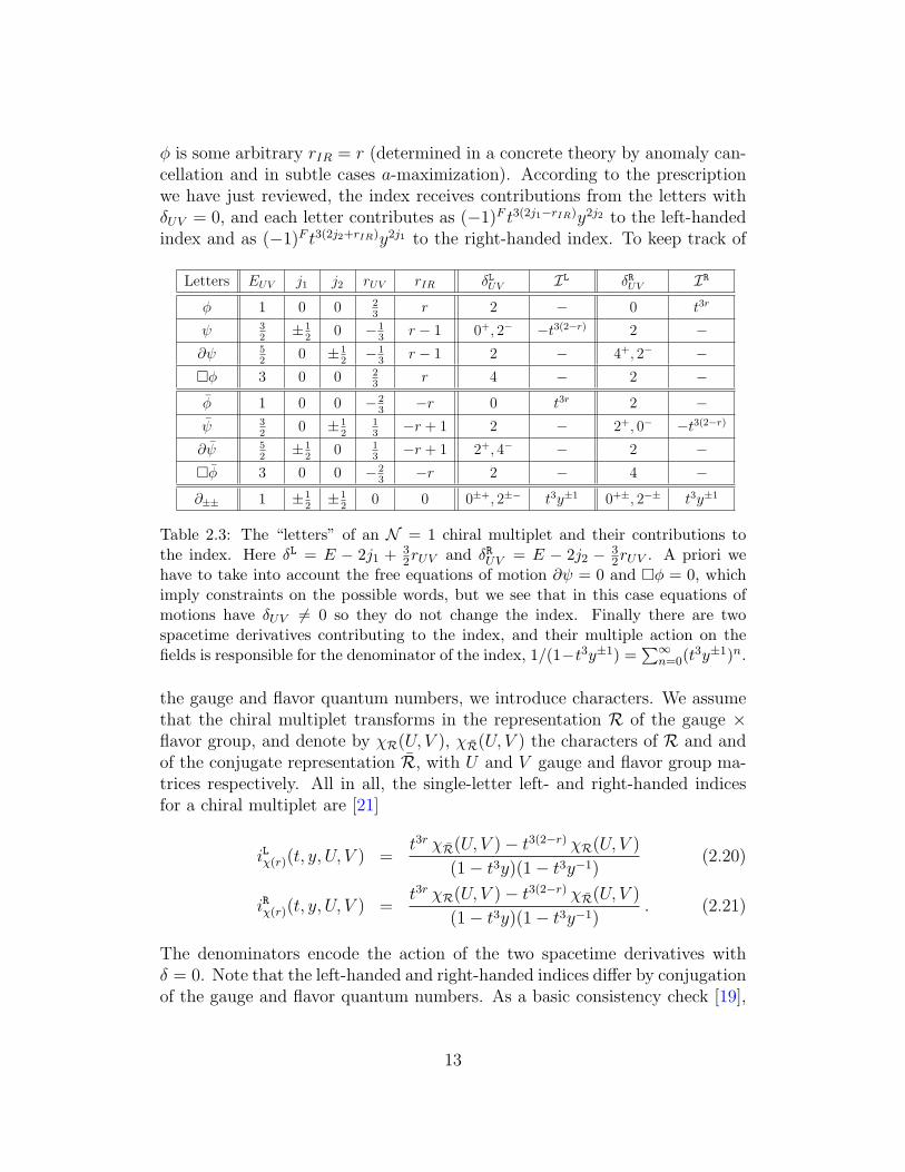
ϕ is some arbitrary rIR = r (determined in a concrete theory by anomaly can-cellation and in subtle cases a-maximization). According to the prescriptionwe have just reviewed, the index receives contributions from the letters withδUV = 0, and each letter contributes as (−1)F t3(2j1−rIR)y2j2 to the left-handedindex and as (−1)F t3(2j2+rIR)y2j1 to the right-handed index. To keep track of
Letters EUV j1 j2 rUV rIR δLUV IL δRUV IR
ϕ 1 0 0 23
r 2 − 0 t3r
ψ 32
±12
0 −13
r − 1 0+, 2− −t3(2−r) 2 −∂ψ 5
20 ±1
2−1
3r − 1 2 − 4+, 2− −
ϕ 3 0 0 23
r 4 − 2 −
ϕ 1 0 0 −23
−r 0 t3r 2 −ψ 3
20 ±1
213
−r + 1 2 − 2+, 0− −t3(2−r)
∂ψ 52
±12
0 13
−r + 1 2+, 4− − 2 −ϕ 3 0 0 −2
3−r 2 − 4 −
∂±± 1 ±12
±12
0 0 0±+, 2±− t3y±1 0+±, 2−± t3y±1
Table 2.3: The “letters” of an N = 1 chiral multiplet and their contributions tothe index. Here δL = E − 2j1 +
32rUV and δRUV = E − 2j2 − 3
2rUV . A priori wehave to take into account the free equations of motion ∂ψ = 0 and ϕ = 0, whichimply constraints on the possible words, but we see that in this case equations ofmotions have δUV = 0 so they do not change the index. Finally there are twospacetime derivatives contributing to the index, and their multiple action on thefields is responsible for the denominator of the index, 1/(1−t3y±1) =
∑∞n=0(t
3y±1)n.
the gauge and flavor quantum numbers, we introduce characters. We assumethat the chiral multiplet transforms in the representation R of the gauge ×flavor group, and denote by χR(U, V ), χR(U, V ) the characters of R and andof the conjugate representation R, with U and V gauge and flavor group ma-trices respectively. All in all, the single-letter left- and right-handed indicesfor a chiral multiplet are [21]
iLχ(r)(t, y, U, V ) =t3r χR(U, V )− t3(2−r) χR(U, V )
(1− t3y)(1− t3y−1)(2.20)
iRχ(r)(t, y, U, V ) =t3r χR(U, V )− t3(2−r) χR(U, V )
(1− t3y)(1− t3y−1). (2.21)
The denominators encode the action of the two spacetime derivatives withδ = 0. Note that the left-handed and right-handed indices differ by conjugationof the gauge and flavor quantum numbers. As a basic consistency check [19],
13
consider a single free massive chiral multiplet (no gauge or flavor indices). Inthe UV, we neglect the mass deformation and as always rUV = 2
3. In the IR,
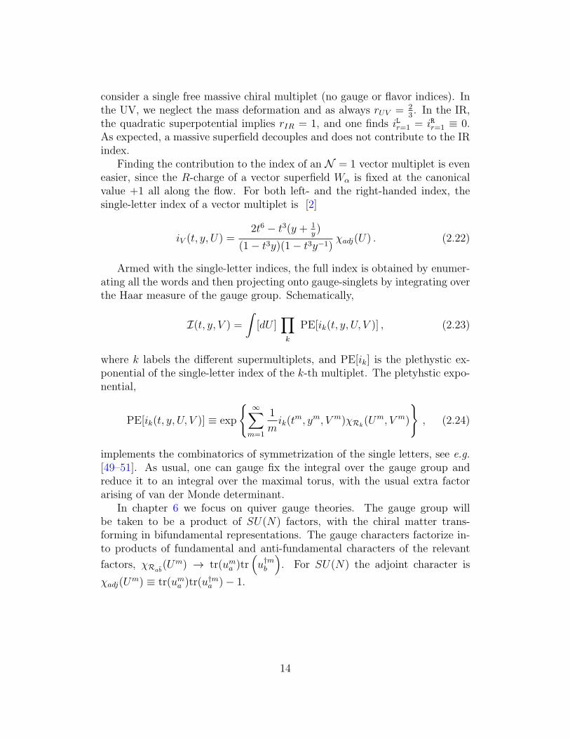
the quadratic superpotential implies rIR = 1, and one finds iLr=1 = iRr=1 ≡ 0.As expected, a massive superfield decouples and does not contribute to the IRindex.
Finding the contribution to the index of an N = 1 vector multiplet is eveneasier, since the R-charge of a vector superfield Wα is fixed at the canonicalvalue +1 all along the flow. For both left- and the right-handed index, thesingle-letter index of a vector multiplet is [2]
iV (t, y, U) =2t6 − t3(y + 1
y)
(1− t3y)(1− t3y−1)χadj(U) . (2.22)
Armed with the single-letter indices, the full index is obtained by enumer-ating all the words and then projecting onto gauge-singlets by integrating overthe Haar measure of the gauge group. Schematically,
I(t, y, V ) =
∫[dU ]
∏k
PE[ik(t, y, U, V )] , (2.23)
where k labels the different supermultiplets, and PE[ik] is the plethystic ex-ponential of the single-letter index of the k-th multiplet. The pletyhstic expo-nential,
PE[ik(t, y, U, V )] ≡ exp
∞∑
m=1
1
mik(t
m, ym, V m)χRk(Um, V m)
, (2.24)
implements the combinatorics of symmetrization of the single letters, see e.g.[49–51]. As usual, one can gauge fix the integral over the gauge group andreduce it to an integral over the maximal torus, with the usual extra factorarising of van der Monde determinant.
In chapter 6 we focus on quiver gauge theories. The gauge group willbe taken to be a product of SU(N) factors, with the chiral matter trans-forming in bifundamental representations. The gauge characters factorize in-to products of fundamental and anti-fundamental characters of the relevant
factors, χRab(Um) → tr(uma )tr
(u†mb
). For SU(N) the adjoint character is
χadj(Um) ≡ tr(uma )tr(u
†ma )− 1.
14
2.3 A universal result about N = 2 → N = 1
flows
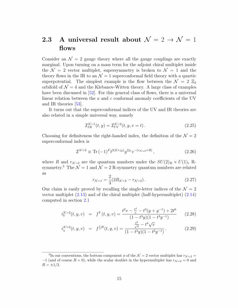
Consider an N = 2 gauge theory where all the gauge couplings are exactlymarginal. Upon turning on a mass term for the adjoint chiral multiplet insidethe N = 2 vector multiplet, supersymmetry is broken to N = 1 and thetheory flows in the IR to an N = 1 superconformal field theory with a quarticsuperpotential. The simplest example is the flow between the N = 2 Z2
orbifold of N = 4 and the Klebanov-Witten theory. A large class of exampleshave been discussed in [52]. For this general class of flows, there is a universallinear relation between the a and c conformal anomaly coefficients of the UVand IR theories [53].
It turns out that the superconformal indices of the UV and IR theories arealso related in a simple universal way, namely
IN=1IR (t, y) = IN=2
UV (t, y, v = t) . (2.25)
Choosing for definiteness the right-handed index, the definition of the N = 2superconformal index is
IN=2 ≡ Tr (−1)F t2(E+j2)y2j1v−(rN=2+R) , (2.26)
where R and rN=2 are the quantum numbers under the SU(2)R × U(1)r R-symmetry.5 The N = 1 and N = 2 R-symmetry quantum numbers are relatedas
rN=1 =2
3(2RN=2 − rN=2) . (2.27)
Our claim is easily proved by recalling the single-letter indices of the N = 2vector multiplet (2.13) and of the chiral multiplet (half-hypermultiplet) (2.14)computed in section 2.1
iN=2V (t, y, v) = fV (t, y, v) =
t2v − t4
v− t3(y + y−1) + 2t6
(1− t3y)(1− t3y−1)(2.28)
iN=2χ (t, y, v) = f
12H(t, y, v) =
t2√v− t4
√v
(1− t3y)(1− t3y−1). (2.29)
5In our conventions, the bottom component ϕ of the N = 2 vector multiplet has rN=2 =−1 (and of course R = 0), while the scalar doublet in the hypermultiplet has rN=2 = 0 andR = ±1/2.
15
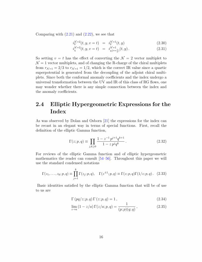
Comparing with (2.21) and (2.22), we see that
iN=2V (t, y, v = t) = iN=1
V (t, y) (2.30)
iN=2χ (t, y, v = t) = iN=1
χ(r= 12)(t, y) . (2.31)
So setting v = t has the effect of converting the N = 2 vector multiplet toN = 1 vector multiplets, and of changing the R-charge of the chiral multipletsfrom rN=1 = 2/3 to rN=1 = 1/2, which is the correct IR value since a quarticsuperpotential is generated from the decoupling of the adjoint chiral multi-plets. Since both the conformal anomaly coefficients and the index undergo auniversal transformation between the UV and IR of this class of RG flows, onemay wonder whether there is any simple connection between the index andthe anomaly coefficients.
2.4 Elliptic Hypergeometric Expressions for the
Index
As was observed by Dolan and Osborn [21] the expressions for the index canbe recast in an elegant way in terms of special functions. First, recall thedefinition of the elliptic Gamma function,
Γ(z; p, q) ≡∏j,k≥0
1− z−1 pj+1qk+1
1− z pjqk. (2.32)
For reviews of the elliptic Gamma function and of elliptic hypergeometricmathematics the reader can consult [54–56]. Throughout this paper we willuse the standard condensed notations
Γ(z1, . . . , zk; p, q) ≡k∏
j=1
Γ(zj ; p, q), Γ(z±1; p, q) ≡ Γ(z; p, q)Γ(1/z; p, q) . (2.33)
Basic identities satisfied by the elliptic Gamma function that will be of useto us are
Γ (pq/z; p, q) Γ (z; p, q) = 1 , (2.34)
limz→a
(1− z/a) Γ(z/a; p, q) =1
(p; p)(q; q), (2.35)
16
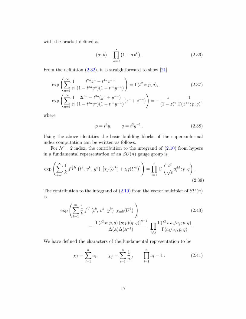
with the bracket defined as
(a; b) ≡∞∏k=0
(1− a bk
). (2.36)
From the definition (2.32), it is straightforward to show [21]
exp
(∞∑n=1
1
n
t2nzn − t4nz−n
(1− t3nyn)(1− t3ny−n)
)= Γ(t2 z; p, q), (2.37)
exp
(∞∑n=1
1
n
2t6n − t3n(yn + y−n)
(1− t3nyn)(1− t3ny−n)(zn + z−n)
)= − z
(1− z)21
Γ(z±1; p, q),
where
p = t3y, q = t3y−1 . (2.38)
Using the above identities the basic building blocks of the superconformalindex computation can be written as follows.
For N = 2 index, the contribution to the integrand of (2.10) from hypersin a fundamental representation of an SU(n) gauge group is
exp
(∞∑k=1
1
kf
12H(tk, vk, yk
) [χf (U
k) + χf (Uk)])
=n∏
i=1
Γ
(t2√va±1i ; p, q
).
(2.39)
The contribution to the integrand of (2.10) from the vector multiplet of SU(n)is
exp
(∞∑k=1
1
kfV(tk, vk, yk
)χadj(U
k)
)(2.40)
=[Γ(t2 v; p, q) (p; p)(q; q)]
n−1
∆(a)∆(a−1)
∏i=j
Γ(t2 v ai/aj; p, q)
Γ(ai/aj; p, q).
We have defined the characters of the fundamental representation to be
χf =n∑
i=1
ai, χf =n∑
i=1
1
a i,
n∏i=1
ai = 1 . (2.41)
17
The character of the adjoint representation is
χadj = χf χf − 1 =∑i =j
ai/aj + n− 1 . (2.42)
We have also defined
∆(a) =∏i=j
(ai − aj) . (2.43)
The Haar measure is given by∮SU(n)
dµ(a)f(a) =1
n!
∮Tn−1
n−1∏i=1
dai2πi ai
∆(a)∆(a−1)f(a)
∣∣∣∣∣∏ni=1 ai=1
, (2.44)
where T is the unit circle. Whenever we gauge a symmetry we have a vectormultiplet associated to the integrated group and thus we will use the followingnotation
Fa Ga ≡ [2 Γ(t2 v; p, q)κ]n−1
n!
×∮Tn−1
n−1∏i=1
dai2πi ai
∏i=j
Γ(t2 v ai/aj; p, q)
Γ(ai/aj; p, q)F (a) G
(a−1)∣∣∣∣∣∏n
i=1 ai=1
,
(2.45)
where κ ≡ (p; p)(q; q)/2. In what follows for the sake of brevity we will omitthe parameters p and q from the elliptic Gamma function, i.e. Γ(x) shouldalways be understood as Γ(x; p, q).
Similarly in N = 1 theories, a chiral superfield in the bifundamental rep-resentation of SU(N1)×SU(N2), and with IR R-charge equal to r can berewritten as
PE[ir(t, y, U)] ≡N1∏i=1
N2∏j=1
Γ(t3r ziw−1j ; t3y, t3/y), (2.46)
Here zk, k = 1, . . . N1, and wk, k = 1, . . . N2, are complex numbers ofunit modulus, obeying
∏N1
k=1 zk =∏N2
k=1wk = 1, which parametrize the Cartansubalgebras of SU(N1) and SU(N2). The multi-letter contribution of a vectormultiplet in the adjoint of SU(N) combines with the SU(N) Haar measure to
18
give the compact expression [15, 21]
κN−1
N !
∮Tn−1
N−1∏i=1
dzi2πi zi
∏k =ℓ
1
Γ(zk/zℓ; p, q). . . . (2.47)
The dots indicate that this is to be understood as a building block of the fullmatrix integral. This equation can also be obtained by setting v = t in (2.40).The numerator factor
∏i=j Γ(t
3 ai/aj; p, q) becomes 1 becuase of the propertyof elliptic Gamma function (2.35).
2.5 4d Index as a path integral on S3 × S1
The superconformal index,
I(t, y, v) = Tr(−1)F t2(E+j2)y2 j1v−(r+R) , (2.48)
doesn’t depend on the couplings of the theory and hence it can be calculatedin the weak coupling limit. The entire contribution to the supersymmetricpartition function on S3×S1 thus comes from the saddle point approximation.One loop partition function of a 4d gauge theory on S3 × S1 was computedin [51] in the presence of fugacities associated with various conserved charges.To compute the superconformal index, we only allow fugacities for chargeswhich commute with Q; i.e. t, y and v.
For the one loop computation in SU(N) gauge theory, it is convenient touse the Coulomb gauge ∂iA
i = 0 where i, j, k are S3 coordinates and ∂i arecovariant derivatives. The residual gauge freedom is fixed by imposing ∂0α = 0where α = 1
V
∫S3 A0 and V is the volume of S3. The partition function is then
written as
Z =
∫dα∆2
∫DA∆1e
−S(A,α) , (2.49)
where ∆1 and ∆2 are Fadeev-Popov determinants associated with the firstand second gauge fixing conditions respectively. For a charge s that commuteswith Q, we can add a supersymmetric coupling with a constant backgroundgauge field as
S → S +
∫d4x sµχµ, (2.50)
where sµ is associated conserved current. χµ is take to be a (χ, 0, 0, 0) and χ
19
is identified with the chemical potential for charge s. The chemical potentialis related to the fugacity, say x, of the Hamiltonian formalism as x = e−βχ. Inour case, x can be any of the t, y and v.
After performing∫DA, one gets an SU(N) unitary matrix model
Z =
∫[dU ]e−Seff [U ] , (2.51)
where U = eiβα and β is the circumference of the circle, [dU ] is the invariantHaar measure on the group SU(N). The Seff is just the one appears in (2.10)
Seff [U ] =∞∑
m=1
1
m
∑j
fRj(tm, ym, vm)χRj(Um, V m) . (2.52)
Here, V denotes the chemical potential that couples to the Cartan of the flavorgroup; Rj labels the representation of the fields under gauge and flavor groupsand fRj is the single letter index of the fields in representation Rj.
The circumference β of the circle is related to the fugacity t as t = e−β/3.To produce the partition function of dimensionally reduced gauge theory onS3 [33, 40] we also scale v = e−β/3, y = 1, and take the limit β → 0. Inappendix C we restore the additional deformations by defining v = e−β(1/3+u)
and set y = e−βη where u and η are chemical potentials for fugacities v and yrespectively. The partition function of 3d gauge theories on squashed S3 wascomputed in [57], the η deformation is related to the squashing parameter ofS3.
20
Chapter 3
S-duality and Two DimensionalTopological Field Theory
Electric-magnetic duality (S-duality) in four-dimensional gauge theory has adeep connection with two-dimensional modular invariance. The canonical ex-ample is the SL(2,Z) symmetry of N = 4 super-Yang-Mills, which can beinterpreted as the modular group of a torus. A physical picture for this corre-spondence is provided by the existence of the six-dimensional (2, 0) supercon-formal field theory, whose compactification on a torus of modular parameterτ yields N = 4 SYM with holomorphic coupling τ (see [58] for a recent dis-cussion).
Gaiotto [3] has discovered a beautiful generalization of this construction.A large class of N = 2 SCFTs (class S SCFTs) in 4d is obtained by compact-ifying a twisted version of the (2, 0) theory on a Riemann surface Σ, of genusg and with n punctures. The complex structure moduli space Tg,n/Γg,n of Σ isidentified with the space of exactly marginal couplings of the 4d theory. Themapping class group Γg,n acts as the group of generalized S-duality transfor-mations of the 4d theory. A striking correspondence between the Nekrasov’sinstanton partition function [12] of the 4d theory and Liouville field theoryon Σ has been conjectured in [9] and further explored in [10, 59–69]. Accord-ing to the celebrated AGT conjecture [9–11], the 4d partition functions onthe Ω-background [12] and on S4 [13] are computed by Liouville/Toda theoryon C. Relations to string/M theory have been discussed in [70–73]. See also[52, 74, 75].
In this chapter we apply the superconformal index to this class of 4d SCFT-s. The index is invariant under continuous deformations of the theory, and isalso expected to be invariant under the S-duality group Γg,n. Assuming S-duality, this implies that the index must be computed by a topological QFTliving on Σ. The usual physical arguments involving the (2, 0) theory give a
21
“proof” of this assertion, as follows. The path integral representation of theindex (2.49) uplifts to a (suitably twisted) path integral of the (2, 0) theory onS3 × S1 × Σ. This path integral must be independent of the metric on Σ. Inthe limit of small Σ we recover the 4d definition; in the opposite limit of largeΣ we expect a purely 2d description. Each puncture on Σ should be regardedas an operator insertion. By this logic, the index must be equal to the n-pointcorrelation function of some TQFT on Σ. The question is whether one candescribe this TQFT more directly, and in the process check the S-duality ofthe index.
It is likely that a “microscopic” Lagrangian formulation of the 2d TQFTmay be derived from the dimensional reduction of the twisted (2, 0) theory thatwe have just described, but we will postpone the discussion in chapter 4. Wewill first write the concrete expression of the index for Gaiotto’s A1 theoriesin this chapter, which always have a 4d Lagrangian description. We show insection 3.1 that the index does indeed take the form expected for a correlator ina 2d TQFT1. We then evaluate explicitly the structure constants and metricof the TQFT operator algebra, and check its associativity, which is the 2dcounterpart of S-duality (section 3.1.2). The metric and structure constantshave elegant expressions in terms of elliptic Gamma functions and the indexin terms of elliptic Beta integrals, a set of special functions which are a newand active branch of mathematical research, see e.g. [54–56] and referencestherein. For Gaiotto’s A1 theories associativity of the topological algebra (andthus S-duality) hinges on the invariance of a special case of the E(5) ellipticBeta integral under the Weyl group of F4. A proof of this symmetry can befound on the math ArXiv [76]. In a related physical context, elliptic identitieshave been used in [21] (following [19]) to prove equality of the superconformalindex for Seiberg-dual pairs of N = 1 gauge theories.
What distinguishes the A1 theories from their counterparts with An≥2 isthat in all duality frames they have a Lagrangian description. This makesit easy to compute their superconformal index explicitly and to identify thestructure constants of the 2d TQFT. The situation for the generalized quivertheories with higher rank gauge groups is qualitatively different: in some du-ality frames the quivers contain intrinsically strongly-coupled blocks with noLagrangian description. The prototypical example of this phenomenon wasdiscussed by Argyres and Seiberg [28]2: the SYM theory with SU(3) gaugegroup and Nf = 6 fundamental hypermultiplets has a dual description involv-ing the strongly-coupled SCFT with E6 flavor symmetry [29]. In the absence
1We thank Abhijit Gadde, Elli Pomoni, Shlomo Razamat and Leonardo Rastelli forletting us use material from their paper [15].
2See also [77] for more examples.
22
of a Lagrangian description for the E6 SCFT, it seems difficult to computeits superconformal index and to define the TQFT structure for generalizedquivers with SU(3) gauge groups.
We solve this problem in the second half of this chapter. By demandingconsistency with Argyres-Seiberg duality, we are able to write down an explicitintegral expression for the index of the E6 SCFT (equation (3.41)). Techni-cally, this is possible thanks to a remarkable inversion formula for a class ofintegral transforms [78]. By construction, the resulting expression for the in-dex is guaranteed to be invariant under an SU(6) ⊗ SU(2) subgroup of theE6 flavor symmetry. The index is seen a posteriori to be invariant under thefull E6 symmetry, providing an independent check of Argyres-Seiberg dualityitself.3 We proceed to define a TQFT structure for generalized quivers withSU(3) gauge symmetries. We check associativity of the operator algebra insection 3.2.3, which is equivalent to a check of S-duality for Gaiotto’s A2 the-ories. Most of our checks are performed perturbatively, to several orders inan expansion in the chemical potentials that enter the definition of the in-dex. Conversely, S-duality implies that associativity must hold exactly, so asa by-product of our analysis we conjecture new identities between integrals ofelliptic Gamma functions.
3.1 The Index in A1 Theories
We start this section by recalling the basics of Gaiotto’s analysis [3]. The mainachievement of [3] is a purely four-dimensional construction of the SCFT im-plicitly defined by compactifying the AN−1 (2, 0) theory on Σ. In the A1 casean explicit Lagrangian description is available, in terms of a generalized quiverwith gauge group SU(2)NG , see figure 3.1 for examples. The internal edges ofa diagram correspond to the SU(2) gauge groups, the external legs to SU(2)flavor groups and the the cubic vertices to chiral fields in the trifundamentalrepresentation (fundamental under each of the groups joining at the vertex).The corresponding Riemann surface is immediately pictured by thickening thelines of the graph into tubes – with the external tubes assumed to be infinitelylong, so that they can be viewed as punctures. The plumbing parameters τiof the tubes are identified with the holomorphic gauge couplings; the degen-eration limit when the surface develops a long tube corresponds to the weakcoupling limit τ → +i∞ of the corresponding gauge group (figure 3.2). Thedifferent patterns of degenerations (pair-of-pants decompositions) of a surfaceΣ of genus g and NF punctures give rise to the different connected diagrams
3For earlier checks of Argyres-Seiberg duality see [79] and [80].
23
(a) (b)
Figure 3.1: (a) Generalized quiver diagrams representing N = 2 superconformaltheories with gauge group SU(2)6 and no flavor symmetries (NG = 6, NF = 0).There are five different theories of this kind. The internal lines of a diagram representand SU(2) gauge group and the trivalent vertices the trifundamental chiral matter.(b) Generalized quiver diagrams for NG = 3, NF = 3. Each external leg representsan SU(2) flavor group. The upper left diagram corresponds the N = 2 Z3 orbifoldof N = 4 SYM with gauge group SU(2).
(a) (b)
Figure 3.2: An example of a degeneration of a graph and appearance of flavourpunctures. As one of the gauge coupling is taken to zero the corresponding edgebecomes very long. Cutting the edge, each of the two resulting semi-infinite openlegs will be associated to chiral matter in an SU(2) flavor representation. In thispicture setting the coupling of the middle legs in (a) to zero gives two copies ofthe theory represented in (b), namely an SU(2) gauge theory with a chiral field inthe bifundamental representation of the gauge group and in the fundamental of aflavour SU(2).
24
with NF external legs (SU(2) flavor groups) and NG = NF +3(g− 1) internallines (SU(2) gauge groups). Since the mapping class group permutes the di-agrams, the associated field theories must be related by generalized S-dualitytransformations [3]. In the higher AN−1 cases the 4d theories are genericallydescribed by more complicated quivers that involve new exotic isolated SCFTsas elementary building blocks.
3.1.1 2d TQFT from the Superconformal Index
For the A1 generalized quivers the index can be explicitly computed as a matrixintegral (2.10),
I =∫ ∏
ℓ∈G [dUℓ] exp(∑∞
n=11n
[∑i∈G f
Vn χadj(U
ni ) +
∑(i,j,k)∈V f
12Hn χ3f (U
ni , U
nj , U
nk )])
.
(3.1)
Here fVn = fV (tn, yn, vn) and f
12H
n = f12H(tn, yn, vn), with fV (t, y, v) and
f12H(t, y, v) the “single-letter partition functions” for respectively the adjoint
and trifundamental degrees of freedom, multiplying the corresponding SU(2)
characters. The explicit expressions for fV and f12H hav already been given
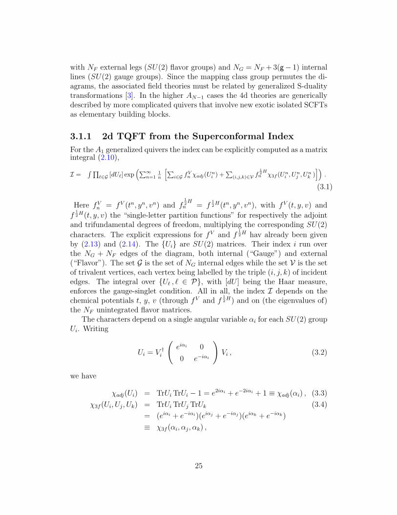
by (2.13) and (2.14). The Ui are SU(2) matrices. Their index i run overthe NG + NF edges of the diagram, both internal (“Gauge”) and external(“Flavor”). The set G is the set of NG internal edges while the set V is the setof trivalent vertices, each vertex being labelled by the triple (i, j, k) of incidentedges. The integral over Uℓ , ℓ ∈ P, with [dU ] being the Haar measure,enforces the gauge-singlet condition. All in all, the index I depends on thechemical potentials t, y, v (through fV and f
12H) and on (the eigenvalues of)
the NF unintegrated flavor matrices.The characters depend on a single angular variable αi for each SU(2) group
Ui. Writing
Ui = V †i
(eiαi 0
0 e−iαi
)Vi , (3.2)
we have
χadj(Ui) = TrUiTrUi − 1 = e2iαi + e−2iαi + 1 ≡ χadj(αi) , (3.3)
χ3f (Ui, Uj, Uk) = TrUiTrUj TrUk (3.4)
= (eiαi + e−iαi)(eiαj + e−iαj)(eiαk + e−iαk)
≡ χ3f (αi, αj, αk) ,
25
where we have used the fact that 2 ∼ 2. Integrating over Vi, the Haar measuresimplifies to ∫
[dUi] =1
π
∫ 2π
0
dαi sin2 αi ≡∫dαi∆(αi) . (3.5)
We now define
Cαiαjαk≡ exp
(∞∑n=1
1
nf
12H
n · χ3f (nαi, nαj, nαk)
), (3.6)
ηαiαj ≡ exp
(∞∑n=1
1
nfVn · χadj(nαi)
)δ(αi, αj) ≡ ηαi δ(αi, αj),
where δ(α, β) ≡ ∆−1(α)δ(α − β) (with the understanding that α and β aredefined modulo 2π) is the delta-function with respect to the measure (3.5).Further define the “contraction” of an upper and a lower α labels as
A...α...B...α... ≡∫ 2π
0
dα∆(α)A...α...B...α... . (3.7)
The superconformal index (3.1) can then be suggestively written as
I =∏
i,j,k∈V
Cαiαjαk
∏m,n∈G
ηαmαn . (3.8)
The internal labels αi , i ∈ G associate to the gauge groups are contracted,while the NF external labels associated to the flavor groups are left open. Theexpression (3.8) is naturally interpreted as an NF -point “correlation function”⟨α1 . . . αNF
⟩g, evaluated by regarding the generalized quiver as a “Feynmandiagram”. The Feynman rules assign to each trivalent vertex the cubic cou-pling Cαβγ , and to each internal propagator the inverse metric ηαβ. S-dualityimplies that the superconformal indices calculated from two diagrams withthe same (NF , NG) must be equal. These properties can be summarized inthe statement that the superconformal index is evaluated by a 2d TopologicalQFT (TQFT).
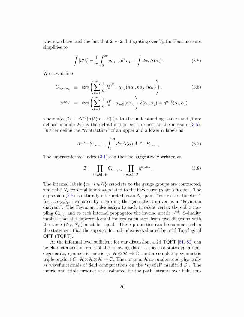
At the informal level sufficient for our discussion, a 2d TQFT [81, 82] canbe characterized in terms of the following data: a space of states H; a non-degenerate, symmetric metric η: H ⊗ H → C; and a completely symmetrictriple product C: H⊗H⊗H → C. The states in H are understood physicallyas wavefunctionals of field configurations on the “spatial” manifold S1. Themetric and triple product are evaluated by the path integral over field con-
26
|α〉
|β〉
|γ〉
|α〉
|β〉
(a) (b)
Figure 3.3: (a) Topological interpretation of the structure constants Cαβγ ≡⟨C| |α⟩|β⟩|γ⟩. The path integral over the sphere with three boundaries defines⟨C| ∈ H∗ ⊗H∗ ⊗H∗. (b) Analogous interpretation of the metric ηαβ ≡ ⟨η||α⟩|β⟩,with ⟨η| ∈ H∗ ⊗H∗, in terms of the sphere with two boundaries.
figurations on the sphere with respectively two and three boundaries (figure3.3). The 2d surfaces where the TQFT is defined are assumed to be oriented,so the S1 boundaries inherit a canonical orientation. To a boundary of inverseorientation (with respect to the canonical one) is associated the dual space H∗.Choosing a basis for H, we can specify the metric and triple product in termsof ηαβ ≡ η(|α⟩, |β⟩) and Cαβγ ≡ C(|α⟩, |β⟩, |γ⟩), or
η =∑α,β
ηαβ⟨α|⟨β| , C =∑α,β,γ
Cαβγ⟨α|⟨β|⟨γ| . (3.9)
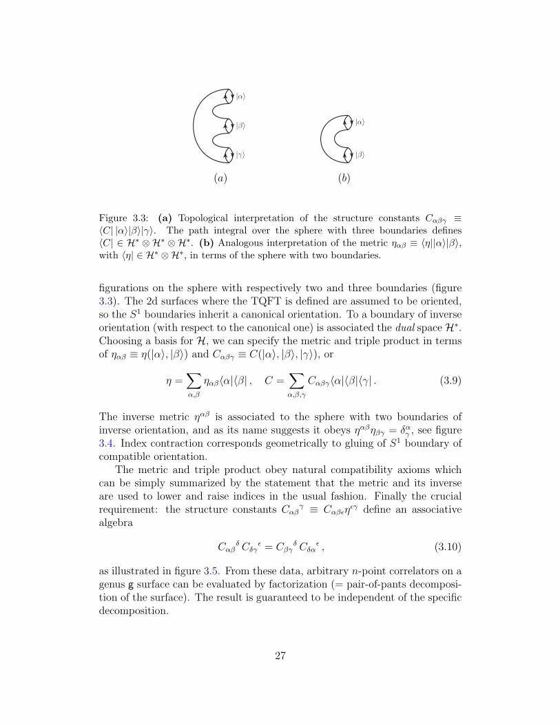
The inverse metric ηαβ is associated to the sphere with two boundaries ofinverse orientation, and as its name suggests it obeys ηαβηβγ = δαγ , see figure3.4. Index contraction corresponds geometrically to gluing of S1 boundary ofcompatible orientation.
The metric and triple product obey natural compatibility axioms whichcan be simply summarized by the statement that the metric and its inverseare used to lower and raise indices in the usual fashion. Finally the crucialrequirement: the structure constants Cαβ
γ ≡ Cαβϵηϵγ define an associative
algebra
Cαβδ Cδγ
ϵ = Cβγδ Cδα
ϵ , (3.10)
as illustrated in figure 3.5. From these data, arbitrary n-point correlators on agenus g surface can be evaluated by factorization (= pair-of-pants decomposi-tion of the surface). The result is guaranteed to be independent of the specificdecomposition.
27
〈α|
〈β|
|α〉
〈γ|
〈γ| |α〉=
(a) (b)
Figure 3.4: Topological interpretation of (a) the inverse metric ηαβ , (b) the relationηαβη
βγ = δγα. By convention, we draw the boundaries associated with upper indicesfacing left and the boundaries associated with the lower indices facing right.
|α〉
|β〉
|γ〉
〈ǫ| =
|α〉
|β〉
|γ〉
〈ǫ|
Figure 3.5: Pictorial rendering of the associativity of the algebra.
In our case the space H is spanned by the states |α⟩ , α ∈ [0, 2π), where αparametrizes the SU(2) eigenvalues, equ.(3.2). Alternatively we may “Fouriertransform” to the basis of irreducible SU(2) representations, |RK⟩ , K ∈ Z+,see appendix A.1. We have concrete expressions (3.6, 3.7) for the cubic cou-plings Cαβγ and for the inverse metric ηαβ, which are manifestly symmetricunder permutations of the indices. Formal inversion of (3.7) gives the metricηαβ ≡ (ηα)−1δ(α, β). Finally with the help of (3.7) we can raise, lower andcontract indices at will. On physical grounds we expect these formal manip-ulations to make sense, since the superconformal index is well-defined as aseries expansion in the chemical potential t, which should have a finite radiusof convergence [2]. The explicit analysis of sections 3.1.2 will confirm theseexpectations. We will find expressions for the index as analytic functions ofthe chemical potentials. Our definitions satisfy the axioms of a 2d TQFT byconstruction, and independently of the specific form of the functions fV (t, y, v)
and f12H(t, y, v), except for the associativity axiom, which is completely non-
trivial. Associativity of the 2d topological algebra is equivalent to 4d S-duality,and it can only hold for very special choices of field content, encoded in thesingle-letter partition functions fV and f
12H .
28
3.1.2 Associativity of the Algebra
In this section we determine explicitly the structure constants and the metricof the TQFT and write them in terms of elliptic Beta integrals. With thehelp of a mathematical result [76] we prove analytically the associativity ofthe topological algebra.
Explicit Evaluation of the Index
α
β
γ
δ
θ
α γ
θ
β δ
=
Figure 3.6: The basic S-duality channel-crossing. The two diagrams are two equiv-alent (S-dual) ways to represent the N = 2 gauge theory with a single gauge groupSU(2) and four SU(2) flavour groups, which is the basic building block of the A1
generalized quiver theories. The indices on the edges label the eigenvalues of thecorresponding SU(2) groups.
As shown in (2.13) and (2.14), the single letter partition function in (t, y, v)parametrization are given by
adjoint : fV (t, y, v) =t2v − t4
v− t3(y + y−1) + 2t6
(1− t3 y)(1− t3y−1), (3.11)
trifundamental : f12H(t, y, v) =
t2√v− t4
√v
(1− t3 y)(1− t3y−1). (3.12)
We are now ready to check explicitly the basic S-duality move – S-duality withrespect to one of the SU(2) gauge groups, represented graphically as channel-crossing with respect to one of the edges of the graph (figure 3.6). The fullS-duality group of a graph is generated by repeated applications of the basicmove to different edges. The contribution to the index from the left graph in
29
figure 3.6 is
I =
∫dθ∆(θ)e
∑∞n=1
1n
[fVn χadj(nθ)+f
12Hn χ3f (nα,nβ,nθ)+f
12Hn χ3f (nθ,nγ,nδ)
].
(3.13)
Substituting the expressions for the characters,
I =e∑∞
n=1
fVnn
π
∫ 2π
0
dθ sin2 θ e
∑∞n=1
[2fV
nn cos 2nθ+
8f
12H
nn (cosnα cosnβ+cosnγ cosnδ) cosnθ
],
(3.14)
where fVn ≡ fV (tn, yn, vn) and f
12H
n ≡ f12H(tn, yn, vn). S-duality of the index
is the statement this integral is invariant under permutations of the externallabels α, β, γ, δ. Since symmetries under α ↔ β and (independently) underγ ↔ δ are manifest, the non-trivial requirement is symmetry under β ↔ γ,which gives the index associated to the crossed graph on the right of figure3.6.
The integrand of (3.14) is not invariant under β ↔ γ, but the integral is, asonce can check order by order in a series expansion in the chemical potential t.Here is how things work to the first non-trivial order. We expand the integrandin t around t = 0, and set y = v = 1 for simplicity. The single-letter partitionfunctions behave as
fV (t, y = 1, v = 1) ∼ t2 − 2 t3 , f12H(t, y = 1, v = 1) ∼ t2 − t4 . (3.15)
The first non-trivial check is for the coefficient of I of order O(t4),
I ∼ t4∫ 2π
0
dθ sin2 θ
(cos 4θ + 2 cos2 2θ + 4A2 cos 2θ (3.16)
+32A21 cos
2 θ − 2 cos 2θ + 16A1 cos θ cos 2θ − 8A1 cos θ
),
where An ≡ cosnα cosnβ+cosnγ cosnδ. Performing the elementary integrals,
I ∼ t4 [6π + 2π (cos 2α+ cos 2β + cos 2γ + cos 2δ + 8 cosα cosβ cos γ cos δ)] ,
(3.17)
which is indeed symmetric under α ↔ β ↔ γ ↔ δ. We stress that crossingsymmetry depends crucially on the specific form of the single-letter partitionfunctions (2.13) and (2.14) and thus on the specific field content. We haveperformed systematic checks by calculating the series expansion to several
30
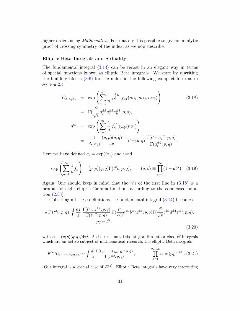
higher orders using Mathematica. Fortunately it is possible to give an analyticproof of crossing symmetry of the index, as we now describe.
Elliptic Beta Integrals and S-duality
The fundamental integral (3.14) can be recast in an elegant way in termsof special functions known as elliptic Beta integrals. We start by rewritingthe building blocks (3.6) for the index in the following compact form as insection 2.4
Cαiαjαk= exp
(∞∑n=1
1
nf
12H
n χ3f (nαi, nαj, nαk)
)(3.18)
= Γ(t2√va±1i a±1
j a±1k ; p, q),
ηαi = exp
(∞∑n=1
1
nfVn χadj(nαi)
)
=1
∆(αi)
(p; p)(q; q)
4πΓ(t2 v; p, q)
Γ(t2 v a±2i ; p, q)
Γ(a±2i ; p, q)
.
Here we have defined ai = exp(iαi) and used
exp
(∞∑n=1
1
nfn
)= (p; p)(q; q)Γ(t2v; p, q), (a; b) ≡
∞∏k=0
(1− abk) (3.19)
Again, One should keep in mind that the rhs of the first line in (3.18) is aproduct of eight elliptic Gamma functions according to the condensed nota-tion (2.33).
Collecting all these definitions the fundamental integral (3.14) becomes
κΓ(t2v; p, q
) ∮ dz
z
Γ(t2 v z±2; p, q)
Γ(z±2; p, q)Γ(
t2√va±1b±1z±1; p, q)Γ(
t2√vc±1d±1z±1; p, q),
pq = t6 ,
(3.20)
with κ ≡ (p; p)(q; q)/4πi. As it turns out, this integral fits into a class of integralswhich are an active subject of mathematical research, the elliptic Beta integrals
E(m)(t1, . . . , t2m+6) ∼∮dz
z
Γ(t1z, . . . t2m+6z; p, q)
Γ(z±2; p, q),
2m+6∏k=1
tk = (pq)m+1
. (3.21)
Our integral is a special case of E(5). Elliptic Beta integrals have very interesting
31
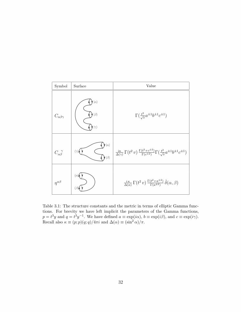
Symbol Surface Value
Cαβγ
|α〉
|β〉
|γ〉
Γ( t2√va±1b±1c±1)
C γαβ
|α〉
|β〉
〈γ| iκ∆(γ)
Γ(t2 v) Γ(t2 v c±2)Γ(c±2)
Γ( t2√va±1b±1c±1)
ηαβ
〈α|
〈β|
i κ∆(α)
Γ(t2 v) Γ(t2 v a±2)Γ(a±2)
δ(α, β)
Table 3.1: The structure constants and the metric in terms of elliptic Gamma func-tions. For brevity we have left implicit the parameters of the Gamma functions,p = t3y and q = t3y−1. We have defined a ≡ exp(iα), b ≡ exp(iβ), and c ≡ exp(iγ).Recall also κ ≡ (p; p)(q; q)/4πi and ∆(α) ≡ (sin2 α)/π.
32
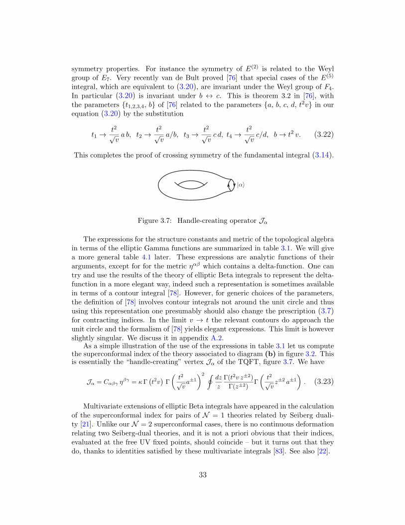
symmetry properties. For instance the symmetry of E(2) is related to the Weylgroup of E7. Very recently van de Bult proved [76] that special cases of the E(5)
integral, which are equivalent to (3.20), are invariant under the Weyl group of F4.In particular (3.20) is invariant under b ↔ c. This is theorem 3.2 in [76], withthe parameters t1,2,3,4, b of [76] related to the parameters a, b, c, d, t2v in ourequation (3.20) by the substitution
t1 →t2√va b, t2 →
t2√va/b, t3 →
t2√vc d, t4 →
t2√vc/d, b→ t2 v. (3.22)
This completes the proof of crossing symmetry of the fundamental integral (3.14).
|α〉
Figure 3.7: Handle-creating operator Jα
The expressions for the structure constants and metric of the topological algebrain terms of the elliptic Gamma functions are summarized in table 3.1. We will givea more general table 4.1 later. These expressions are analytic functions of theirarguments, except for for the metric ηαβ which contains a delta-function. One cantry and use the results of the theory of elliptic Beta integrals to represent the delta-function in a more elegant way, indeed such a representation is sometimes availablein terms of a contour integral [78]. However, for generic choices of the parameters,the definition of [78] involves contour integrals not around the unit circle and thususing this representation one presumably should also change the prescription (3.7)for contracting indices. In the limit v → t the relevant contours do approach theunit circle and the formalism of [78] yields elegant expressions. This limit is howeverslightly singular. We discuss it in appendix A.2.
As a simple illustration of the use of the expressions in table 3.1 let us computethe superconformal index of the theory associated to diagram (b) in figure 3.2. Thisis essentially the “handle-creating” vertex Jα of the TQFT, figure 3.7. We have
Jα = Cαβγ ηβγ = κΓ
(t2v)Γ
(t2√va±1
)2 ∮dz
z
Γ(t2v z±2)
Γ(z±2)Γ
(t2√vz±2 a±1
). (3.23)
Multivariate extensions of elliptic Beta integrals have appeared in the calculationof the superconformal index for pairs of N = 1 theories related by Seiberg duali-ty [21]. Unlike our N = 2 superconformal cases, there is no continuous deformationrelating two Seiberg-dual theories, and it is not a priori obvious that their indices,evaluated at the free UV fixed points, should coincide – but it turns out that theydo, thanks to identities satisfied by these multivariate integrals [83]. See also [22].
33
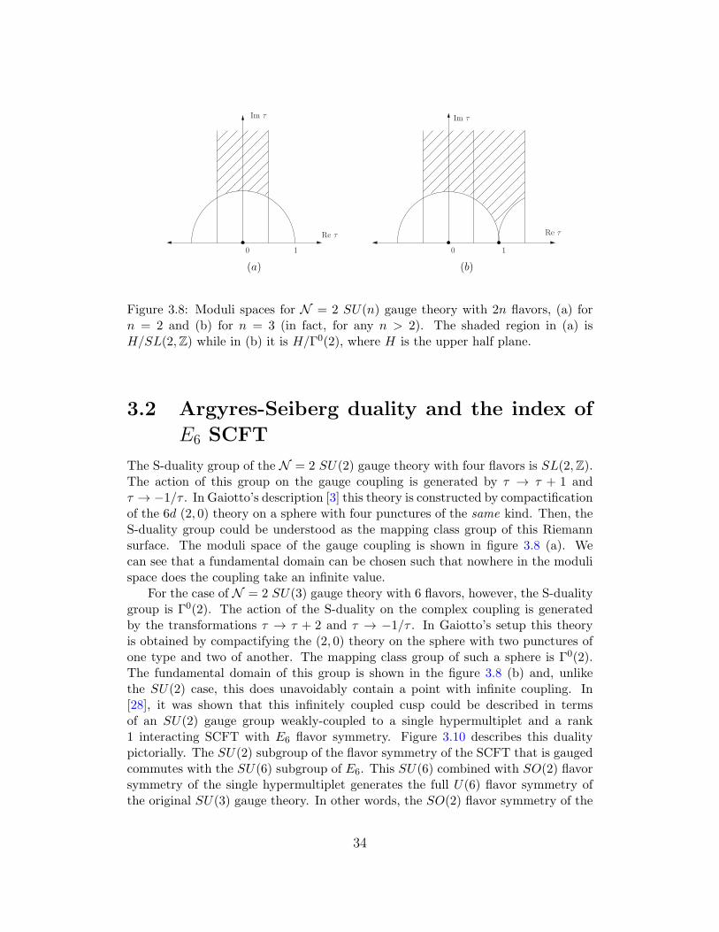
Re τ
Im τ
0 1 10
Re τ
Im τ
(a) (b)
Figure 3.8: Moduli spaces for N = 2 SU(n) gauge theory with 2n flavors, (a) forn = 2 and (b) for n = 3 (in fact, for any n > 2). The shaded region in (a) isH/SL(2,Z) while in (b) it is H/Γ0(2), where H is the upper half plane.
3.2 Argyres-Seiberg duality and the index of
E6 SCFT
The S-duality group of the N = 2 SU(2) gauge theory with four flavors is SL(2,Z).The action of this group on the gauge coupling is generated by τ → τ + 1 andτ → −1/τ . In Gaiotto’s description [3] this theory is constructed by compactificationof the 6d (2, 0) theory on a sphere with four punctures of the same kind. Then, theS-duality group could be understood as the mapping class group of this Riemannsurface. The moduli space of the gauge coupling is shown in figure 3.8 (a). Wecan see that a fundamental domain can be chosen such that nowhere in the modulispace does the coupling take an infinite value.
For the case of N = 2 SU(3) gauge theory with 6 flavors, however, the S-dualitygroup is Γ0(2). The action of the S-duality on the complex coupling is generatedby the transformations τ → τ + 2 and τ → −1/τ . In Gaiotto’s setup this theoryis obtained by compactifying the (2, 0) theory on the sphere with two punctures ofone type and two of another. The mapping class group of such a sphere is Γ0(2).The fundamental domain of this group is shown in the figure 3.8 (b) and, unlikethe SU(2) case, this does unavoidably contain a point with infinite coupling. In[28], it was shown that this infinitely coupled cusp could be described in termsof an SU(2) gauge group weakly-coupled to a single hypermultiplet and a rank1 interacting SCFT with E6 flavor symmetry. Figure 3.10 describes this dualitypictorially. The SU(2) subgroup of the flavor symmetry of the SCFT that is gaugedcommutes with the SU(6) subgroup of E6. This SU(6) combined with SO(2) flavorsymmetry of the single hypermultiplet generates the full U(6) flavor symmetry ofthe original SU(3) gauge theory. In other words, the SO(2) flavor symmetry of the
34
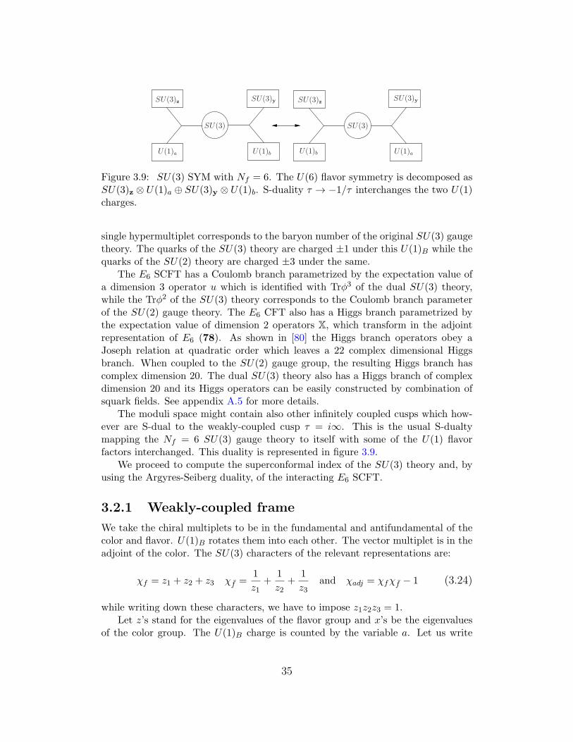
SU(3)y
U(1)bU(1)a
SU(3) SU(3)
U(1)b U(1)a
SU(3)z SU(3)y SU(3)z
Figure 3.9: SU(3) SYM with Nf = 6. The U(6) flavor symmetry is decomposed asSU(3)z ⊗ U(1)a ⊕ SU(3)y ⊗ U(1)b. S-duality τ → −1/τ interchanges the two U(1)charges.
single hypermultiplet corresponds to the baryon number of the original SU(3) gaugetheory. The quarks of the SU(3) theory are charged ±1 under this U(1)B while thequarks of the SU(2) theory are charged ±3 under the same.
The E6 SCFT has a Coulomb branch parametrized by the expectation value ofa dimension 3 operator u which is identified with Trϕ3 of the dual SU(3) theory,while the Trϕ2 of the SU(3) theory corresponds to the Coulomb branch parameterof the SU(2) gauge theory. The E6 CFT also has a Higgs branch parametrized bythe expectation value of dimension 2 operators X, which transform in the adjointrepresentation of E6 (78). As shown in [80] the Higgs branch operators obey aJoseph relation at quadratic order which leaves a 22 complex dimensional Higgsbranch. When coupled to the SU(2) gauge group, the resulting Higgs branch hascomplex dimension 20. The dual SU(3) theory also has a Higgs branch of complexdimension 20 and its Higgs operators can be easily constructed by combination ofsquark fields. See appendix A.5 for more details.
The moduli space might contain also other infinitely coupled cusps which how-ever are S-dual to the weakly-coupled cusp τ = i∞. This is the usual S-dualtymapping the Nf = 6 SU(3) gauge theory to itself with some of the U(1) flavorfactors interchanged. This duality is represented in figure 3.9.
We proceed to compute the superconformal index of the SU(3) theory and, byusing the Argyres-Seiberg duality, of the interacting E6 SCFT.
3.2.1 Weakly-coupled frame
We take the chiral multiplets to be in the fundamental and antifundamental of thecolor and flavor. U(1)B rotates them into each other. The vector multiplet is in theadjoint of the color. The SU(3) characters of the relevant representations are:
χf = z1 + z2 + z3 χf =1
z1+
1
z2+
1
z3and χadj = χfχf − 1 (3.24)
while writing down these characters, we have to impose z1z2z3 = 1.Let z’s stand for the eigenvalues of the flavor group and x’s be the eigenvalues
of the color group. The U(1)B charge is counted by the variable a. Let us write
35
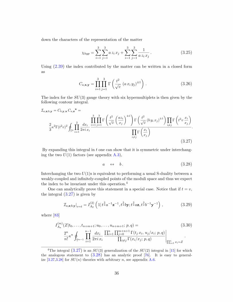
down the characters of the representation of the matter
χhyp =3∑
i=1
3∑j=1
a zi xj +3∑
i=1
3∑j=1
1
a zi xj. (3.25)
Using (2.39) the index contributed by the matter can be written in a closed formas
Ca,x,y =3∏
i=1
3∏j=1
Γ
(t2√v(a xi yj)
±1
). (3.26)
The index for the SU(3) gauge theory with six hypermultiplets is then given by thefollowing contour integral.
Ia,z;b,y = Cb,y,x Ca,zx =
2
3κ2Γ(t2v)2
∮T2
2∏i=1
dxi2πi xi
3∏i=1
3∏j=1
Γ
(t2√v
(azixj
)±1)Γ
(t2√v(b yi xj)
±1
)∏i =j
Γ
(t2v
xixj
)∏i =j
Γ
(xixj
) .
(3.27)
By expanding this integral in t one can show that it is symmetric under interchang-ing the two U(1) factors (see appendix A.3),
a ↔ b . (3.28)
Interchanging the two U(1)s is equivalent to performing a usual S-duality between aweakly-coupled and infinitely-coupled points of the moduli space and thus we expectthe index to be invariant under this operation.4
One can analytically prove this statement in a special case. Notice that if t = v,the integral (3.27) is given by
Ia,z;b,y|v=t = I(2)A2
(1| t
32a−1z−1, t
32 by; t
32az, t
32 b−1y−1
), (3.29)
where [83]
I(m)An
(Z|t0, . . . , tn+m+1;u0, . . . , un+m+1; p, q) = (3.30)
2n
n!κn∮Tn−1
n−1∏i=1
dxi2πi xi
∏ni=1
∏m+n+1j=0 Γ(tj xi, uj/xi; p, q)∏
i =j Γ(xi/xj ; p, q)
∣∣∣∣∣∏ni=1 xi=Z
.
4The integral (3.27) is an SU(3) generalization of the SU(2) integral in [15] for whichthe analogous statement to (3.28) has an analytic proof [76]. It is easy to general-ize [3.27,3.28] for SU(n) theories with arbitrary n, see appendix A.6.
36
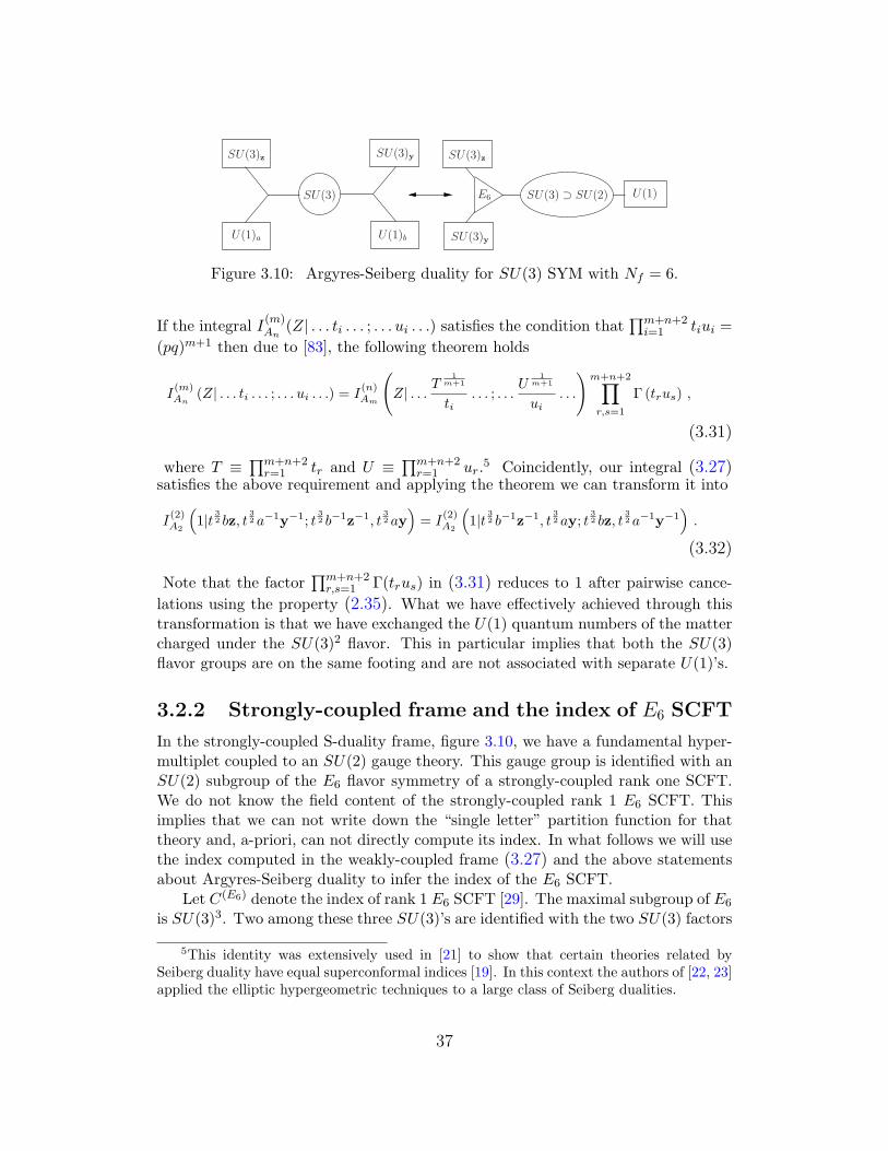
U(1)bU(1)a
SU(3) U(1)SU(3) ⊃ SU(2)E6
SU(3)z SU(3)y SU(3)z
SU(3)y
Figure 3.10: Argyres-Seiberg duality for SU(3) SYM with Nf = 6.
If the integral I(m)An
(Z| . . . ti . . . ; . . . ui . . .) satisfies the condition that∏m+n+2
i=1 tiui =
(pq)m+1 then due to [83], the following theorem holds
I(m)An
(Z| . . . ti . . . ; . . . ui . . .) = I(n)Am
(Z| . . . T
1m+1
ti. . . ; . . .
U1
m+1
ui. . .
)m+n+2∏r,s=1
Γ (trus) ,
(3.31)
where T ≡∏m+n+2
r=1 tr and U ≡∏m+n+2
r=1 ur.5 Coincidently, our integral (3.27)
satisfies the above requirement and applying the theorem we can transform it into
I(2)A2
(1|t 3
2 bz, t32 a−1y−1; t
32 b−1z−1, t
32 ay
)= I
(2)A2
(1|t 3
2 b−1z−1, t32 ay; t
32 bz, t
32 a−1y−1
).
(3.32)
Note that the factor∏m+n+2
r,s=1 Γ(trus) in (3.31) reduces to 1 after pairwise cance-
lations using the property (2.35). What we have effectively achieved through thistransformation is that we have exchanged the U(1) quantum numbers of the mattercharged under the SU(3)2 flavor. This in particular implies that both the SU(3)flavor groups are on the same footing and are not associated with separate U(1)’s.
3.2.2 Strongly-coupled frame and the index of E6 SCFT
In the strongly-coupled S-duality frame, figure 3.10, we have a fundamental hyper-multiplet coupled to an SU(2) gauge theory. This gauge group is identified with anSU(2) subgroup of the E6 flavor symmetry of a strongly-coupled rank one SCFT.We do not know the field content of the strongly-coupled rank 1 E6 SCFT. Thisimplies that we can not write down the “single letter” partition function for thattheory and, a-priori, can not directly compute its index. In what follows we will usethe index computed in the weakly-coupled frame (3.27) and the above statementsabout Argyres-Seiberg duality to infer the index of the E6 SCFT.
Let C(E6) denote the index of rank 1 E6 SCFT [29]. The maximal subgroup of E6
is SU(3)3. Two among these three SU(3)’s are identified with the two SU(3) factors
5This identity was extensively used in [21] to show that certain theories related bySeiberg duality have equal superconformal indices [19]. In this context the authors of [22, 23]applied the elliptic hypergeometric techniques to a large class of Seiberg dualities.
37
in the flavor group of the weakly-coupled theory, see figure 3.10. Let the additionalSU(3) be denoted byw. The fundamental representation of E6 is decomposed underSU(3)w ⊗ SU(3)y ⊗ SU(3)z as,
27E6 = (3, 3,1)⊕ (3,1,3)⊕ (1,3, 3) . (3.33)
Thus, the character of the E6 fundamental fields is,
χ27 =
3∑i,j=1
(wi
yj+ziwj
+yizj
),
3∏i=1
yi =
3∏i=1
zi =
3∏i=1
wi = 1 . (3.34)
The index C(E6) is thus a function of w, y, and z. The S-duality picture suggeststhat we should decompose SU(3)w as SU(2)e ⊗U(1)r. This amounts to the changeof variables w1, w2, w2 → er, re ,
1r2, for which the character of the fundamental
of E6 becomes
χ27 = (er +r
e+
1
r2)(
1
y1+
1
y2+
1
y3) + (
1
er+e
r+ r2)(z1 + z2 + z3) +
3∑i,j=1
yizj.
(3.35)
Thus, the index of the E6 SCFT can be denoted as C(E6) ((e, r),y, z). In the abovenotations the index of the additional hypermultiplet of the theory is
Cs, e = Γ
(t2√ve±1 s±1
). (3.36)
Thus, one can write the superconformal index of the theory in the strongly-coupled frame as
I (s, r;y, z) = CseC
(E6)(e,r),y,z (3.37)
= κΓ(t2v)
∮T
de
2πi e
Γ(t2ve±2)
Γ(e±2)Γ(
t2√ve±1 s±1) C(E6) ((e, r),y, z) .
By Argyres-Seiberg duality we have to equate
I (s, r;y, z) = Ia,z;b,y , (3.38)
where Ia,z;b,y is given in (3.27), and we appropriately identify the U(1) charges,
s = (a/b)3/2, r = (a b)−1/2 . (3.39)
It so happens that the integral of equation (3.37) has special properties whichallow us to invert it (see appendix A.4 and [78] for the details). One can write the
38
following
κ
∮Cw
ds
2πi s
Γ(√v
t2w±1 s±1)
Γ( vt4, s±2)
I (s, r;y, z) = Γ(t2v w±2) C(E6) ((w, r),y, z) ,
(3.40)
where the contour Cw is a deformation of the unit circle such that it encloses s =√v
t2w±1 and excludes s = t2√
vw±1 (for precise definition and details see appendix A.4
and [78]). The above expression for the index C(E6) does satisfy (3.37), but a-prioridoes not uniquely follow from it. However, as we will explicitly see below, (3.40) isconsistent with what is expected from E6 SCFT. We will comment on this issue inthe end of this section. We can thus use the Argyres-Seiberg duality (3.38) to writea closed form expression for the E6 index
C(E6) ((w, r),y, z) =2κ3Γ(t2v)2
3Γ(t2v w±2)
∮Cw
ds
2πi s
Γ(√v
t2 w±1 s±1)
Γ( vt4 , s
±2)×
×∮T2
2∏i=1
dxi2πi xi
3∏i=1
3∏j=1
Γ
t2√v
(s
13 zixj r
)±1Γ
t2√v
(s−
13 yi xjr
)±1∏
i =j
Γ
(t2v
xixj
)∏i =j
Γ
(xixj
) .
(3.41)One can rewrite the above expression without using the special integration contour.The integration contour Cw can be split into five pieces: a contour around the unit
circle T, two contours encircling the simple poles of Γ(√v
t2w±1 s±1) at s =
√v
t2w±1, and
two contours encircling in the opposite direction the simple poles of Γ(√v
t2w±1 s±1)
at t2√vw±1. Using the fact that elliptic Gamma function satisfies (2.35) we have
C(E6) ((w, r),y, z) =κ
Γ(t2vw±2)
∮T
ds
s
Γ(√v
t2w±1 s±1)
Γ( vt4, s±2)
I (s, r;y, z)
+1
2
Γ(w−2)
Γ(t2vw−2)
[I(s =
√vw
t2, r;y, z
)+ I
(s =
t2√vw
, r;y, z
)]+
1
2
Γ(w2)
Γ(t2vw2)
[I(s =
√v
t2w, r;y, z
)+ I
(s =
t2w√v, r;y, z
)].
(3.42)
The index (3.41) encodes some information about the matter content of the E6
theory. To extract this information it is useful to expand the index (3.41) in the
39
chemical potentials. We define an expansion in t as
C(E6) ≡∞∑k=0
ak tk . (3.43)
The first several orders in this expansion have the following form
a0 =1
a1t =a2t2 = a3t
3 = 0
a4t4 =
t4
vχE678
a5t5 =0
a6t6 =− t6χE6
78 − t6 + t6v3
a7t7 =
t7
v
(y +
1
y
)χE678 +
t7
v
(y +
1
y
)− t7v2
(y +
1
y
)a8t
8 =t8
v2
(χE6
sym2(78)− χE6
650 − 1)+ t8v + t8v
a9t9 =− t9
(y +
1
y
)χE678 − 2t9
(y +
1
y
)+ t9v3
(y +
1
y
)a10t
10 =− t10
v(χE6
78 χE678 − χE6
650 − 1) +t10
v
(y2 + 1 +
1
y2
)χE678+
+t10
v
(y +
1
y
)2
− t10v2(y +
1
y
)2
a11t11 =
t11
v2
(y +
1
y
)(χE6
78 χE678 − χE6
650 − 1) + t11v
(y +
1
y
)+ t11v
(y +
1
y
).
(3.44)
The adjoint representation of E6 , 78, decomposes in the following way in terms ofits maximal SU(3)3 subgroup
78 = (3,3,3) + (3, 3, 3) + (8,1,1) + (1,8,1) + (1,1,8) , (3.45)
and 650 of E6 is composed as
650 = 27× 27− 78− 1 . (3.46)
The Higgs branch operators X of E6 theory are in the adjoint (78) representationof E6 flavor algebra. The terms of the index proportional to χE6
78 are forming thefollowing series, [
t4
v− t6 +
t7
v
(y +
1
y
)− t9
(y +
1
y
)+ · · ·
]χE678 , (3.47)
40
which is the index of a multiplet with ∆ = 2, j = j = 0 and r = 0 and of itsderivatives (see appendix C.2 of [42]). Taken as a “letter” this multiplet has thefollowing “single letter” partition function
t4/v − t6
(1− t3y)(1− t3/y), (3.48)
which matches the quantum numbers of the Higgs branch operators on the weakly-coupled side of the Argyres-Seiberg duality if we follow the identifications listed in[80].
The E6 singlet part of the index contains yet another series,
t6v3 − t7v2(y +
1
y
)+ t8v + t9v3
(y +
1
y
)+ · · · . (3.49)
This series forms the index of a chiral multiplet with ∆ = 3, j = j = 0 and r = 3together with its derivatives (appendix C.1 of [42])
t6v3 − t7v2(y + 1
y
)+ t8v
(1− t3y)(1− t3/y). (3.50)
Since the Coulomb branch operator, u, of E6 theory (which is identified as Trϕ3 ofthe dual SU(3) theory) has exactly the same quantum numbers, this multiplet isidentified as the Coulomb branch operator.
The remaining singlet part of the index,
− t6 +t7
v
(y +
1
y
)+ t8v − 2t9
(y +
1
y
)+ · · · , (3.51)
is just the index of the stress tensor multiplet and its derivatives (appendix C.3 of[42])
−t6 + t7
v
(y + 1
y
)+ t8v − t9
(y + 1
y
)(1− t3y)(1− t3/y)
. (3.52)
Besides the matter content, the index also provides possible constraints amongoperators. For example, it was argued [80] that the Higgs branch operators of theE6 theory should obey the Joseph relations,
(X⊗ X)|I2 = 0 , (3.53)
where the representation I2 is defined as
sym2(V (adj)) = V (2adj)⊕ I2 . (3.54)
For E6, adj = 78, 2adj = 2430 and then sym2(78) = 2430 ⊕ 650 ⊕ 1. Thus, in
41
our caseI2 = 650⊕ 1 . (3.55)
The Joseph relation in E6 theory reads,
(X⊗ X)|650⊕1 = 0 , (3.56)
which means that these operators should not appear in the index. The index of Xis t4/v, then the index of X⊗ X is t8/v2. (3.44) shows that our index is consistentwith the Joseph relation.
Further constraints can also be derived from the higher order terms in (3.44).Let us consider the index at order t10. The meaning of each term is clear. The firstterm corresponds to operators X⊗(QX) with the constraintQ(X⊗X)650+1 = 0 whichis a descendant of Joseph relation above (3.56). The last three terms are derivative
descendants of t4
v χE678 ,
t7
v
(y + 1
y
)and −t7v2
(y + 1
y
)respectively. However, terms
of the formt10v2χE6
78 , (3.57)
which would be corresponding to the Higgs⊗Coulomb operators are absent. Thisfact implies the constraint
X⊗ u = 0 . (3.58)
This is consistent with the fact that the E6 theory has rank 1. The absence of− t10
v χE678 also implies the constraint
X⊗ T = 0 , (3.59)
where T is the stress tensor. The structure of the index at order t11 is consistentwith these two constraints.
Finally, let us comment on the uniqueness of our proposal. In principle, theindex (3.41) produced by the construction of this section might differ from the true
index of the E6 SCFT: C(E6)true ((e, r),y, z) = C(E6)((e, r),y, z)+δC((e, r),y, z), with
δC satisfying
∮T
de
2πi e
Γ( t2√ve±1s±1)Γ(t2v e±2)
Γ(e±2)δC((e, r),y, z) = 0 . (3.60)
At this stage we are not able to rigorously rule out such a possibility. However,the E6 covariance of our proposal, its consistency with physical expectations aboutprotected operators and the further S-duality checks performed in the followingsection, make us confident that we have identified the correct index of the E6 SCFT.
Note that the expression for the index (3.41) is not explicitly given in terms ofE6 characters. However, as one learns from the perturbative expansion (3.44), thecharacters of SU(3)y⊗SU(3)z⊗SU(2)w⊗U(1)r always combine into E6 characters.Essentially, since the weakly-coupled frame has really SU(6)⊗U(1) flavor symmetry
42
we can write an expression for the E6 index which has a manifest SU(6) ⊗ SU(2)symmetry,6 but not the full E6. The fact that just by assuming Argyres-Seibergduality we obtain an index for a theory with an E6 flavor symmetry and with aconsistent spectrum of operators is a non-trivial check of Argyres-Seiberg duality.
3.2.3 S-duality checks of the E6 index
In the previous section we have discussed the superconformal index of the Nf = 6SU(3) theory and of its strongly-coupled dual. One can obtain this theory bycompactifying a (2, 0) 6d theory on a sphere with four punctures, two U(1) puncturesand two SU(3) punctures. The different S-duality frames are then given by thedifferent degeneration limits of this Riemann surface. The weakly-coupled framesare obtained by bringing together one of the U(1) punctures and one of the SU(3)punctures, and the strongly-coupled frame is obtained by colliding the two SU(3)(U(1)) punctures. The coupling constant of the theory is related to the cross ratioof the four punctured sphere.
In [3] Gaiotto suggested to generalize this picture by considering general Rie-mann surfaces with an arbitrary numbers of punctures of different types (two typesin case of the SU(3) theories). The claim is that all theories with the same numberand type of punctures and same topology of the Riemann surface are related byS-dualities. The immediate consequence of this claim for the superconformal indexis that all such theories have to have the same index as it is independent of the val-ues of the coupling, i.e. the moduli of the Riemann surface. This implies that thesuperconformal index is a topological invariant of the punctured Riemann surface.It was claimed in [15] that the superconformal index can be actually interpreted asa correlator in a two dimensional topological quantum field theory. The structureconstants of this TQFT are given by the index of the three punctured sphere andthe contraction of indices (i.e. metric) is gauging of the flavor symmetries. Theassociativity of the algebra generated by the structure constants is equivalent to theinvariance of the index of four punctured spheres under pair-of-pants decompositioninto two three punctured spheres. The structure constants and the metric wereconstructed and the associativity was explicitly verified for the SU(2) case.
In this section we will make the same analysis for the SU(3) case. We havetwo types of punctures, associated to U(1) and SU(3) flavor symmetries. There arethus different three point functions one can construct. The index of the theory ona sphere with three SU(3) punctures, i.e. the index of the E6 theory, is a structure
constant which we will denote by C(333)x,y,z and it is just given by (3.41),
C(333)x,y,z = C(E6)
((√x1x2,√x1x2
),y, z
). (3.61)
6The fact that this symmetry can be manifestly seen in the expression for the index isvery reminiscent of the construction of the E6 symmetry using multi-pronged strings in [84].It is very interesting to understand whether these facts are related.
43
This vertex corresponds to the E6 theory which has rank one, and thus we will refer
to it as a rank 1 vertex. We will denote by C(133)x,y,a the index of the sphere with
two SU(3) punctures and one U(1) puncture. This is a free theory consisting ofa hypermultiplet in fundamental of two SU(3) flavor groups and its value is givenby (3.26),
C(133)a,x,y =
3∏i,j=1
Γ
(t2√v(axiyj)
±). (3.62)
This vertex corresponds to a free, rank 0, theory and we will refer to it as rankzero structure constant. Later on we will define yet another three point function,formally associated to a sphere with two U(1) punctures and one SU(3) puncture.This vertex will have effective rank −1. The metric of the model, ηx,y, is defined as
ηx,y =2
3κ2 Γ2(t2v)
∏16i<j63
Γ
(t2v(
xixj
)±)Γ
((xixj
)±) ∆(x−1,y) , (3.63)
where ∆(x−1,y) is a δ-function kernel defined by∮T2
2∏i=1
dxi2πi xi
∆(x,w) f(x) = f(w) , w ∈ T2 . (3.64)
The indices are contracted as follows
A...u...B...u... ≡∮T2
2∏i=1
dui2πiui
A...u...B...u...
∣∣∣∣∣∏3i=1 ui=1
. (3.65)
Following these definitions the superconformal indices of all the SU(3) generalizedquivers are obtained by contracting the structure constants in different ways.
For the S-duality to hold, and subsequently for the structure constants to have aTQFT interpretation, the algebra generated by these objects has to be associative.We proceed to verify this fact.
(333)− (333) associativity
Let us consider the generalized quiver with genus zero and four SU(3) punctures.The index should be invariant under the permutation of the four SU(3) characters,
I3333(x,y;w, z) = C(333)x,y,uη
u,vC(333)v,z,w = C
(333)x,z,uη
u,vC(333)v,y,w . (3.66)
44
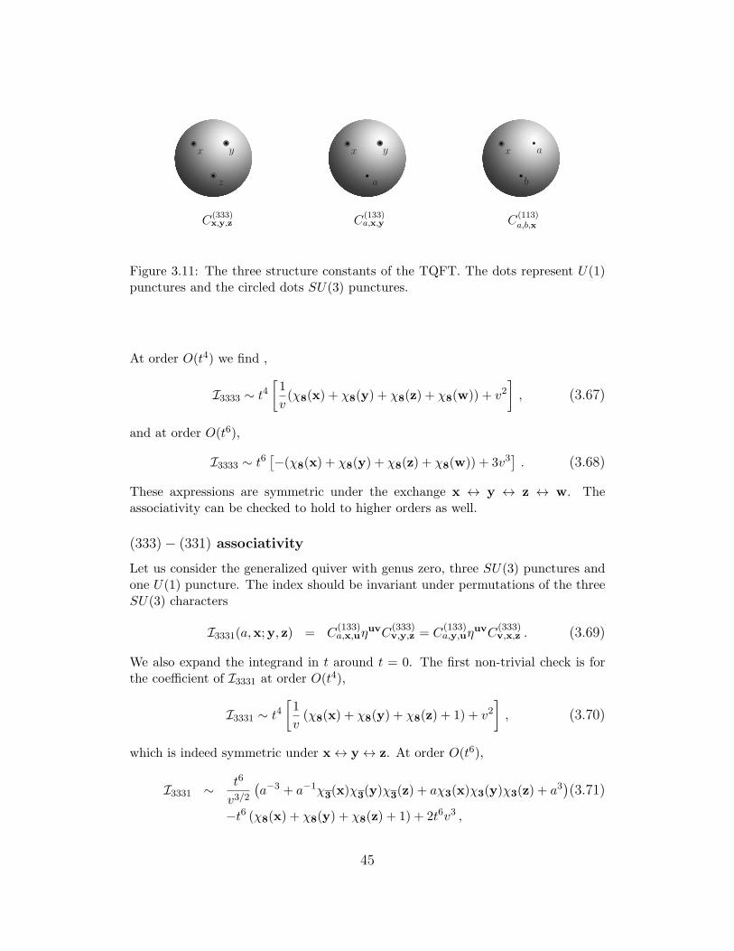
x y
z
x y
a
x a
b
C(333)x,y,z C
(133)a,x,y C
(113)a,b,x
Figure 3.11: The three structure constants of the TQFT. The dots represent U(1)punctures and the circled dots SU(3) punctures.
At order O(t4) we find ,
I3333 ∼ t4[1
v(χ8(x) + χ8(y) + χ8(z) + χ8(w)) + v2
], (3.67)
and at order O(t6),
I3333 ∼ t6[−(χ8(x) + χ8(y) + χ8(z) + χ8(w)) + 3v3
]. (3.68)
These axpressions are symmetric under the exchange x ↔ y ↔ z ↔ w. Theassociativity can be checked to hold to higher orders as well.
(333)− (331) associativity
Let us consider the generalized quiver with genus zero, three SU(3) punctures andone U(1) puncture. The index should be invariant under permutations of the threeSU(3) characters
I3331(a,x;y, z) = C(133)a,x,uη
uvC(333)v,y,z = C
(133)a,y,uη
uvC(333)v,x,z . (3.69)
We also expand the integrand in t around t = 0. The first non-trivial check is forthe coefficient of I3331 at order O(t4),
I3331 ∼ t4[1
v(χ8(x) + χ8(y) + χ8(z) + 1) + v2
], (3.70)
which is indeed symmetric under x ↔ y ↔ z. At order O(t6),
I3331 ∼ t6
v3/2(a−3 + a−1χ3(x)χ3(y)χ3(z) + aχ3(x)χ3(y)χ3(z) + a3
)(3.71)
−t6 (χ8(x) + χ8(y) + χ8(z) + 1) + 2t6v3 ,
45

which is also symmetric under x ↔ y ↔ z. Again, we can perform systematicchecks to arbitrary high order in t.
The (311) three point function and (311)− (331) associativity
The index of the Nf = 6 SU(3) theory in the strongly-coupled frame is given interms of an integral over an SU(2) character. Thus, we can not write it using thestructure constants and the metric we defined in the beginning of this section. Thestrongly-coupled frame is obtained when two U(1) punctures collide and thus inwhat follows we will formally define a structure constant with two U(1) charactersand an SU(3) character such that when contracted with the E6 structure constantusing the metric above it will produce the index of the strongly-coupled frame.
Let us rewrite the index in the strongly-coupled frame,
I (s, r;y, z) = κ Γ(t2v)
∮T
de
2πi e
Γ( t2√ve± s±)
Γ(e±2)Γ(t2v e±2) C ((e, r),y, z) ,
(3.72)
as rank one (E6) (333) and rank −1 (113) vertices contracted
I (a, b;y, z) =C(113)a,b,x η
x,x′C
(333)x′,y,z
=2
3κ2 Γ(t2v)2
∮T2
2∏i=1
dxi2πi xi
∏i =j
Γ(t2v xi/xj)
Γ(xi/xj)C(113)
(a, b,x−1
)C(333) (x,y, z) .
(3.73)
For this we define
C(113)(a, b,x−1
)=
3
2κΓ(t2v)
∮T
de
2πi e
Γ( t2√ve±1 s±1) Γ(t2v e±2)
Γ(e±2)
∏i =j
Γ(xi/xj)
Γ(t2v xi/xj)∆(x,w) .
(3.74)
Here, w = (e, r) with e an SU(2) character and r a U(1) character. The U(1)charges are related as in (3.39), s = (a/b)3/2 and r = (a b)−1/2. ∆(x,w) is a δ-function kernel defined in (3.64). The (113) vertex has effective rank −1. Using theabove definition the TQFT algebra is well defined with all the contractions beingSU(3) integrals.
The associativity of (311) vertex contracted with a (333) vertex is achieved byconstruction: remember that we obtained the index of E6 SCFT by requiring this
46
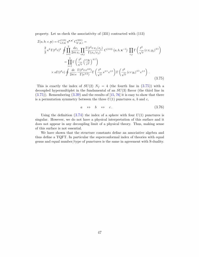
property. Let us check the associativity of (331) contracted with (113)
I(a, b; c,y) = C(113)a,b,x η
x,x′C
(331)x′,y,c =
2
3κ2 Γ(t2v)2
∮ 2∏i=1
dxi2πi xi
∏i =j
Γ(t2v xi/xj)
Γ(xi/xj)C(113)
(a, b,x−1
) ∏i,j
Γ
(t2√v(c xi yj)
±1
)
=3∏
i=1
Γ
(t2√v
(c yir2
)±1)
× κΓ(t2v)
∮de
2πi e
Γ(t2v e±2)
Γ(e±2)Γ
(t2√vs±1 e±1
)Γ
(t2√v(c r yi)
±1e±1
).
(3.75)
This is exactly the index of SU(2) Nf = 4 (the fourth line in (3.75)) with adecoupled hypermultiplet in the fundamental of an SU(3) flavor (the third line in(3.75)). Remembering (3.39) and the results of [15, 76] it is easy to show that thereis a permutation symmetry between the three U(1) punctures a, b and c,
a ↔ b ↔ c . (3.76)
Using the definition (3.74) the index of a sphere with four U(1) punctures issingular. However, we do not have a physical interpretation of this surface and itdoes not appear in any decoupling limit of a physical theory. Thus, making senseof this surface is not essential.
We have shown that the structure constants define an associative algebra andthus define a TQFT. In particular the superconformal index of theories with equalgenus and equal number/type of punctures is the same in agreement with S-duality.
47
x
a b
y
z w
x y x y
z a c
x
b
a
(a) (b) (c) (d)
Figure 3.12: The relevant four-punctured spheres for A2 theories. The three differentdegeneration limits of a four-punctured sphere correspond to different S-dualityframes. For example, in (a) two of the degeneration limits (when a U(1) puncturecollides with an SU(3) puncture) correspond to the weakly-coupled Nf = 6 SU(3)theory, the third limit (when two like punctures collide) corresponds to the Argyres-Seiberg theory. In (d) the degeneration limits correspond to the different dualityframes of SU(2) SYM with Nf = 4 theory plus a decoupled hypermultiplet.
48
Chapter 4
TQFT Structure of the Indexfor An-Type Quivers
In the previous chapter we have showed that the superconformal index is a usefulobservable of Gaiotto class S theories. With the concrete expression of the indexfor Gaiotto’s A1 theories, we demonstrate in section 3.1 that the index does indeedtake the form of a correlator in a 2d TQFT and in the process check the S-duality ofthe index. Then by demanding consistency with Argyres-Seiberg duality, we furtherwrite down an explicit integral expression for the index of the E6 SCFT which hasno Lagrangian description. The spectral information predicted by the E6 indexcoincides with other works. With the index of the E6 SCFT as one of the basiccomponents, we proceed to define a TQFT structure for generalized quivers withSU(3) gauge symmetries and check the associativity and S-duality.
General Four-dimensional superconformal field theories of S [3, 4] arise frompartially-twisted compactification of the six-dimensional (2, 0) theory on a puncturedRiemann surface C. The complex-structure moduli of C are identified with theexactly marginal couplings of the 4d SCFT, while the punctures are associated toflavor symmetries.
Any punctured surface can be obtained, usually in more than one way, by glu-ing three-punctured spheres (pairs of pants) with cylinders. The three-puncturedspheres are then the elementary building blocks. They correspond to isolated 4dSCFTs with flavor symmetry G1 ⊗G2 ⊗ G3, where each factor GI is associated toone of the three punctures.1 The cylinders correspond to N = 2 vector multiplets,and the gluing operation amounts to gauging a common SU(k) symmetry of twopunctures. The gluing parameter is interpreted as the complexified gauge coupling,with zero coupling corresponding to an infinitely long cylinder – a degenerationlimit of the surface. Different pairs-of-pants decompositions of the same surface
1In this chapter we focus on class S theories that descend from the (2, 0) theory of typeAk−1. Then the punctures are classified by the possible embeddings of SU(2) into SU(k)and GI ⊂ SU(k) is the commutant of the chosen embedding.
49
C correspond to different descriptions of the same SCFT, related by generalizedS-dualities.
As showen in previous chapters the index is naturally viewed as a correlator ina 2d topological QFT living on C. Let us review how this works. We parametrizethe index of a three-punctured sphere as I(a1,a2,a3), where aI are fugacities dualto the Cartan subgroup of GI : except in special cases these are a priori unknownfunctions. On the other hand we can easily write down the “propagator” associatedto a cylinder,
η(a,b) = ∆(a)IV (a) δ(a,b−1) , (4.1)
where ∆(a) is the Haar measure and IV (a) the index of a vector multiplet, whichis known explicitly. The index of a generic theory of class S can be written in termsof the index of these elementary constituents. As the simplest example, gluing twothree-punctured spheres with one cylinder one obtains the index of a four-puncturedsphere,
I(a1,a2,a3,a4) =
∮[da]
∮[db] I(a1,a2,a) η(a,b) I(b,a3,a4) (4.2)
=
∮[da] ∆(a) I(a1,a2,a) IV (a) I(a−1,a3,a4) ,
where we have introduced the notation∮[da] ≡
∮ k−1∏i=1
dai2πiai
. (4.3)
If we expand the index in a convenient basis of functions fα(a), labeled by SU(k)representations α,2 we can associate to each three-punctured sphere “structureconstants” Cαβγ and to each propagator a metric ηαβ ,
I(a,b, c) =∑α,β,γ
Cαβγ fα(a) fβ(b) fγ(c) (4.4)
ηαβ =
∮[da]
∮[db] η(a,b) fα(a) fβ(b) . (4.5)
Invariance of the index under the different ways to decompose the surface is tan-tamount of saying that Cαβγ and ηαβ define a two-dimensional topological QFT.3
2For theories of type A, fα(a) are symmetric functions of their arguments, which arefugacities dual to the Cartan generators of SU(k). More generally, for theories of type Dand E, fα(a) are invariant under the appropriate Weyl group.
3We are using this term somewhat loosely. As axiomatized by Atiyah, a TQFT isunderstood to have a finite-dimensional state-space, while in our case the state-space willbe infinite-dimensional. The best-understood example of a 2d topological theory with aninfinite-dimensional state-space is the zero-area limit of 2d Yang-Mills theory [85, 86] (see
50
The crucial property is associativity,
CαβγCγδϵ = CαδγC
γβϵ , (4.6)
where indices are raised with the metric ηαβ and lowered with the inverse metricηαβ .
It is very natural to choose the complete set of functions fα(a) to be orthonor-mal under the measure that appears in the propagator,∮
[da] ∆(a) IV (a) fα(a)fβ(a−1) = δαβ . (4.7)
Then the metric ηαβ is trivial,
ηαβ = δαβ . (4.8)
Condition (4.7) still leaves considerable freedom, as it is obeyed by infinitely manybases of functions related by orthogonal transformations. The real simplificationarises if we can find an explicit basis fα(a), such that the structure constants arediagonal,
Cαβγ = 0 → α = β = γ . (4.9)
Associativity (4.6) is then automatic. For structure constants satisfying (4.6) onecan always find a basis in which they are diagonal: we give a detailed example ofsuch a diagonalization procedure in appendix B.1 for the simplest limit of the index.The challenge is to describe the basis in concrete form.
In general the measure appearing in the propagator is complicated and no ex-plicit set of orthonormal functions is available. We find it very useful to consider anansatz
fα(a) = K(a)Pα(a) , (4.10)
for some function K(a). Clearly, from (4.7), the functions Pα(a) are orthornormalunder the new measure ∆(a),∮
[da] ∆(a)Pα(a)P β(a−1) = δαβ , ∆(a) ≡ IV (a)K(a)2∆(a) . (4.11)
(Recall that ∆(a) always denotes the Haar measure). The name of the game is tofind a clever choice of K(a), for which ∆(a) is a simple known measure and theorthonormal basis Pα(a) an explicit set of functions such that (4.9) holds.
Once the diagonal basis fα(a) and the structure constant Cααα are known,
e.g. [87] for a comprehensive review). Happily, the 2d topological theory associated to theindex turns out to be closely related to 2d Yang-Mills.
51
one can easily calculate the index of the SCFT associated to the genus g surfacewith s punctures. Such a surface can be built by gluing 2g− 2 + s three-puncturedspheres, so we have4
Ig,s(a1,a2, . . . ,as) =∑α
(Cααα)2g−2+s
s∏I=1
fα(aI) . (4.12)
In the rest of this chapter we implement the following strategy. We start byconsidering the generalized SU(2) quivers. Since they have a Lagrangian descrip-tion, closed form expressions for the index (as matrix integrals) are readily available.We then look for a basis of functions fα(a) that diagonalizes the structure con-stants. Fortunately, for each special limit of the index that we consider, the diagonalbasis is of the form (4.10), with Pα(a) well-known symmetric polynomials: Hall-Littlewood, Schur or Macdonald polynomials. (The first two are in fact special casesof Macdonald polynomials). Since these polynomials are defined for arbitrary rank,we can extrapolate from the SU(2) case and formulate compelling conjectures forthe index of all generalized quivers of type A. (This approach readily generalizes toall ADE theories, but in this paper we focus on the A series). Finally we check ourconjectures against expected symmetry enhancements and S-dualities.
4.1 Limits of the index with additional super-
symmetry
We now consider several limits of the superconformal index, such that the statescontributing to it are annihilated by more than one supercharge. Recall that beforetaking any limit the index receives contributions only from states with
δ1− = E − 2j2 − 2R+ r = 0 , (4.13)
which are annihilated by Q1−. We tend to refer to the different limits of the indexby the type of symmetric polynomials relevant for their evaluation. In appendix B.2we discuss which short multiplets of the superconformal algebra are counted by theindex in each of these limits.
4Here for simplicity we are considering the case where all external punctures are “max-imal”, i.e. they have flavor symmetry SU(k). The prescription for punctures with reducedsymmetry is discussed in detail in sections 4.2, 4.3 and 4.4.
52
Macdonald index
We first consider the limit5
σ → 0 , ρ , τ fixed , (4.14)
(which is the same as p→ 0 with q and t fixed). The limit is well-defined since thepower of σ in the trace formula (2.4) is given by 1
2δ1+ ≥ 0. The index is given by
IM = TrM (−1)F ρ12(E−2j1−2R−r) τ
12(E+2R+2j2+r) (4.15)
= TrM (−1)F q12(E−2j1−2R−r) tR+r ,
where TrM denotes the trace restricted to states with δ1+ = E + 2j1 − 2R− r = 0.Such states are annihilated by Q1+. All in all IM is a 1
4 -BPS object receivingcontributions only from states annihilated by two supercharges, one chiral (Q1+) andone anti-chiral (Q1−). The single letter partition functions of the half-hypermultipletand the vector simplify to
f12H =
τ
1− ρτ=
√t
1− q, fV =
−τ2 − ρτ
1− ρτ=
−t− q
1− q. (4.16)
Hall-Littlewood index
We further specialize the index by sending ρ→ 0, so we are taking the limit
σ → 0 , ρ→ 0 , τ fixed , (4.17)
(equivalently, q , p → 0 with t fixed), which is well-defined thanks to δ1± ≥ 0. Theindex is given by
IHL = TrHL(−1)F τ12(E+2R+2j2+r) = TrHL(−1)F τ2(E−R) , (4.18)
where TrHL denotes the trace restricted to states with δ1± = E ± 2j1 − 2R− r = 0.All in all, taking (4.13) into account, the states contributing to the index obey
j1 = 0 , j2 = r , E = 2R+ r , (4.19)
and are annihilated by three supercharges: Q1+, Q1− and Q1−.Let us consider the Hall-Littlewood (HL) index for a theory with a Lagrangian
description. From table 2.2, we see that it gets contributions only from the scalar qof the hypermultiplet and from the fermion λ1+ of the vector multiplet. The single
5An equivalent limit can be obtained by sending ρ to zero.
53
letter partition function of the half-hypermultiplet and the vector multiplet is then
f12H = τ, fV = −τ2 . (4.20)
Remarkably, for generalized quivers with a sphere topology the computation of theHL index is equivalent to the computation of the partition function over the Higgsbranch discussed in [88, 89] (the Hilbert series of the Higgs branch).6 This can beshown as follows. To compute the partition function of [88, 89] for the Higgs branchof an N = 2 gauge theory one counts all the possible gauge invariant operators builtfrom the scalar components of the hypermultiplets taking into account the F-termsuperpotential constraints. In an N = 2 gauge theory with M SU(2) gauge factorsthe superpotential takes the form
W =
M∑i=1
∑α∈i
Q(α)aiakal
Φaibi Q
(α) biakal , (4.21)
where the summation over i is over the gauged groups. The set i is the set of (atmost two) trifundamental hypermultiplets transforming non-trivially under gaugegroup i. The F-term constraints then read
Q(α1)aiakal
Q(α1)biakal +Q(α2)aiaman Q
(α2)biaman = 0 . (4.22)
If the quiver diagram does not have loops, i.e. the corresponding Riemann surfacehas a topology of a sphere, this is a set ofM independent constraints. It then followsthat the computation of this partition function is the same as the computation ofthe index. Indeed, one associates a fugacity τ for each scalar component of Q. Theconstraint (4.22) is quadratic in Q and is in the adjoint representation of the gaugegroup. It is implemented by multiplying the unconstrained partition function withthe following factor [88, 89],
exp
[−
∞∑n=1
1
nτ2n
(a2ni + a−2n
i + 1)]
= (1− τ2)(1− τ2 a2i )(1− τ2 a−2i ) . (4.23)
This factor is the same as the index of the letter λ1+. Thus, one can think of theletter λ1+ in the calculation of the index as playing the same role as the superpoten-tial constraint in the calculation of the Higgs partition function! This logic can beextended to higher-rank theories, where not all the building blocks have Lagrangiandescription, but the Higgs branch can still be described in terms of operators obey-ing certain constraints. This concludes the argument that the HL index is the sameas the Higgs partition function for theories with sphere topology. Our derivation
6A relation of a similar limit of the N = 1 index with the counting problems discussedin [90, 91] was mentioned in [23]. We thank V. Spiridonov for bringing this reference to ourattention.
54
also makes it clear that this correspondence fails for higher-genus theories.In [88] non-trivial very explicit expressions for the Higgs branch partition func-
tion of the SCFTs with exceptional flavor symmetry groups [29, 92] were conjectured.We will see that they are exactly reproduced by the HL index.
Schur index
The Schur index is defined by specializing the fugacities to ρ = τ with σ arbitrary(equivalently q = t with p arbitrary). It reads
IS = Tr(−1)F σ12(E+2j1−2R−r) ρE−j1+j2 e−β(E−2j2−2R+r) . (4.24)
By construction, all charges in the trace formula commute with the supercharge Q1−“with respect to which” the index is evaluated. From table 2.1, we observe that thecharges in (4.24) also commute with Q1+. Thus the index receives contributionsfrom states with δ1+ = δ1− = 0 (the intersection of the cohomologies of Q1+ and of
Q1−) and it is independent of both σ and β. We can then write
IS = Tr(−1)F ρ2(E−R) = Tr(−1)F qE−R . (4.25)
The Schur index can also be obtained as a special case of the Macdonald indexby setting ρ = τ (equivalently q = t); we have just seen that for ρ = τ the indexbecomes independent of σ so the limit σ → 0 that we take to obtain the Macdonaldindex is immaterial.
The single letter partition functions of the half-hypermultiplets and the vectormultiplet are given by
f12H =
ρ
1− ρ2=
√q
1− q, fV =
−2ρ2
1− ρ2=
−2q
1− q. (4.26)
The Schur index is the same as the index studied in [17], where we referred toit as the reduced index.
Coulomb-branch index
Finally we consider the limit
τ → 0 , ρ , σ fixed , (4.27)
which is well-defined thanks to δ2+ ≥ 0. The trace formula becomes
IC = TrC(−1)F σ12(E+2j1−2R−r) ρ
12(E−2j1−2R−r) e−β(E−2j2−2R+r) , (4.28)
55
where TrC denotes the trace over the states with δ2+ = E + 2j2 + 2R + r = 0,
which are annihilated by Q2+. All in all, the index gets contributions from states
annihilated by two antichiral supercharges, Q1− and Q2+.In this limit the single-letter partition function of the half-hypermultiplet and
the vector multiplet are
f12H = 0, fV = σρ ≡ T . (4.29)
From the viewpoint of the the single-letter partition functions one can take aninteresting less restrictive limit,
τ , σ → 0 , ρ→ ∞ with Q ≡ τρ and T ≡ σρ fixed. (4.30)
In this limit we have
f12H = 0, fV =
T −Q
1−Q. (4.31)
We recover (4.29) for Q → 0. In terms of the new fugacities Q and T the indexreads
ICM = TrCM (−1)F T12(E+2j1−2R−r)Q
12(E+2j2+2R+r) , (4.32)
where TrCM denotes the trace restricted to states satisfying E + 2j1 + r = 0. Thisindex is well-defined for Lagrangian theories and for theories related to them bydualities.
We now describe the explicit evaluation of these special limits of the index forthe SCFTs of class S.
4.2 Hall-Littlewood index
We begin with the Hall-Littlewood index,
IHL(τ) = TrHL(−1)F τ2E−2R , (4.33)
where TrHL denotes the trace restricted to states with j1 = 0 and E − 2R− r = 0.This is the limit that leads to the greatest simplifications.
4.2.1 SU(2) quivers
Let us start from the SU(2) generalized quivers, for which the basic building blocksare known explicitly. There is only one type of non-trivial puncture, the maxi-
56
mal puncture with SU(2) flavor symmetry. The SCFT corresponding the three-punctured sphere, denoted by T2 in [3], is the theory of free hypermultiplets in thetrifundamental representation of SU(2). Its index is immediately evaluated,
I(a, b, c) = PE [τχ1(a)χ1(b)χ1(c)]a,b,c,τ =1∏
sa,sb,sc=±1(1− τ asa bsb csc), (4.34)
where the fugacities a, b, and c label the Cartans of the three SU(2) flavor groups.The plethystic exponent PE is defined as
PE [f(xi)]xi≡ exp
( ∞∑n=1
1
nf(xni )
). (4.35)
We will often omit the subscript xi in the expressions for PE[. . . ]. χ1(a) is thecharacter of fundamental representation of SU(2). More generally the SU(2) Schurpolynomials χλ are given by
χλ(a) =a−1−λ − a1+λ
a−1 − a. (4.36)
The propagator η(a, b) is also easily evaluated:
η(a, b) = ∆(a)IV (a)δ(a, b−1) , (4.37)
where IV (a) is the index of the vector multiplet,
IV (a) = PE[−τ2χ2(a)]a,τ = (1− τ2) (1− τ2 a2) (1− τ2 a−2) , (4.38)
and ∆(a) the SU(2) Haar measure,
∆(a) =1
2(1− a2)(1− 1
a2) . (4.39)
Following the strategy outlined in the beginning of this chapter, we look for a com-plete set of functions fλ(a) orthonormal under the propagator measure such thatthe structure constants are diagonal,
I(a, b, c) =∞∑λ=0
Cλλλ fλ(a)fλ(b)fλ(c) . (4.40)
We describe this calculation in appendix B.1. We find the remarkable result
fλ(a) = K(a) P λHL(a, a
−1|τ), (4.41)
Cλλλ =
√1− τ2 (1 + τ2)
P λHL(τ, τ
−1|τ). (4.42)
57
Here P λHL are the SU(2) Hall-Littlewood polynomials,
P λHL(a, a
−1|τ) = χλ(a)− τ2χλ−2(a) for λ ≥ 1 , P λ=0HL (a, a−1|τ) =
√1 + t2 ,
(4.43)
which are orthonormal under the measure
∆(a) = ∆HL(a) =1
2
(1− a2)(1− a−2)
(1− τ2a2)(1− τ2a−2). (4.44)
The requirement that fλ(a) be orthonormal under the propagator measure ∆(a)IV (a)fixes the prefactor K(a),
K(a) =
(∆HL(a)
∆(a)IV (a)
) 12
=1√
1− τ21
(1− τ2a2)(1− τ2a−2). (4.45)
We can now immediately write down an explicit formula for the index of anygeneralized SU(2) quiver associated to a genus g Riemann surface with s punctures.From (4.12),
Ig,s(a1, a2, . . . , as) =(1− τ2
)g−1 (1 + τ2
)2g−2+s · (4.46)∞∑λ=0
1[P λHL(τ, τ
−1| τ)]2g−2+s
s∏I=1
P λHL(aI , a
−1I | τ)
(1− τ2a2I)(1− τ2a−2I )
.
In particular for genus g with no punctures the sum over the SU(2) irreduciblerepresentations in (4.46) can be explicitly performed and one gets
I(2)g =
(1− τ2
)g−1(τ2g−2 +
(1 + τ2
)g−1 (1− τ2g−2
))1− τ2g−2
. (4.47)
We observe that setting a flavor fugacity a = τ we “close” the correspondingpuncture. For example we can go from the three-punctured sphere to the two-punctured sphere (=cylinder),
I(a1, a2, τ) ∼∑λ
P λHL(a1, a
−11 |τ)P λ
HL(a2, a−12 |τ) = η(a1, a2) . (4.48)
(There is an overall divergent proportionality factor). This procedure of (partially)closing punctures by trading (some of) the flavor fugacities with τ plays an im-portant role, as it will allow us to construct the index for theories with arbitrarytypes of punctures. For SU(k) theories the punctures are classified by the differentembeddings of SU(2) inside SU(k) [3, 4], which are conveniently labelled by aux-iliary Young diagrams with k boxes. For SU(2) we get only two possibilities: (i)a row with two boxes corresponding to the “maximal” puncture with SU(2) flavor
58
symmetry, (ii) a column with two boxes corresponding to the absence of a puncture.For higher-rank theories the space of possibilities will be more interesting.
4.2.2 Higher rank: preliminaries
For higher-rank quivers the situation is more complicated since the basic buildingblocks are given by strongly-interacting SCFTs for which direct computations arenot possible. However, the expressions that we obtained for the index of the SU(2)quivers can be naturally extrapolated to higher rank. The basic conjecture is thatthe set of functions fα(a) that diagonalize the structure constants are related toHall-Littlewood polynomials for higher-rank as well.
The Hall-Littlewood (HL) polynomials associated to U(k) are a set of orthogonalpolynomials labeled by Young diagrams with at most k rows, λ = (λ1, . . . , λk),λj ≥ λj+1. They are given by [93]
P λHL(x1, . . . , xk| τ) = Nλ(τ)
∑σ∈Sk
xλ1
σ(1) . . . xλk
σ(k)
∏i<j
xσ(i) − τ2xσ(j)
xσ(i) − xσ(j), (4.49)
and they are orthonormal under the measure
∆HL =1
k!
∏i=j
1− xi/xj1− τ2xi/xj
. (4.50)
The normalization Nλ(t) is given by
N−2λ1,...λk
(τ) =∞∏i=0
m(i)∏j=1
(1− τ2j
1− τ2
), (4.51)
where m(i) is the number of rows in the Young diagram λ = (λ1, . . . , λk) of lengthi. For SU(k) groups we take Young diagrams with λk = 0 and the product of xkin (4.49) is constrained as
∏ki=1 xk = 1.
Let us also quote from the outset the expression for the SU(k) propagator,
η(a,b−1) = ∆(a)IV (a)δ(a,b−1) , (4.52)
where ∆(a) is the SU(k) Haar measure,
∆(a) =1
k!
∏i=j
(1− ai
aj
),
k∏i
ai = 1 , (4.53)
59
and IV (a) the vector multiplet index,
IV =1
1− τ2
k∏j,i=1
(1− τ2aj/ai) . (4.54)
4.2.3 SU(3) quivers – the E6 SCFT
We now focus on the SU(3) theories. There are two kinds of non-trivial punc-tures: the maximal puncture, associated to the Young diagram (3, 0, 0), which car-ries the full SU(3) flavor symmetry; the puncture associated with the Young diagram(2, 1, 0), which carries U(1) flavor symmetry. The elementary building blocks arethe 333 vertex and the 331 vertex, where 3 and 1 are shorthands for the SU(3) andU(1) punctures, respectively.
The 333 vertex corresponds to the E6 SCFT of [29], denoted by T3 in [3]. Amaximal subgroup of the E6 flavor symmetry is given by SU(3)3 and we parametrizethe Cartans of the three SU(3)s by aI . Guided by the expression of the T2 indexobtained in the previous subsection, we conjecture that the index of T3 is given by
I(a1,a2,a3) =∑λ1,λ2
A(τ)
P λ1,λ2
HL (τ2, τ−2, 1| τ)
3∏I=1
K(aI)Pλ1,λ2
HL (aI | τ) (4.55)
K(a) =1
1− τ2
3∏i,j=1, i =j
1
(1− τ2ai/aj),
3∏i=1
ai = 1 (4.56)
A(τ) = (1− τ4)(1 + τ2 + τ4) . (4.57)
The function K(a) is fixed as always by (4.11), with ∆ = ∆HL, while the overallfugacity-independent normalization factor A(τ) was fixed by comparing with theknown result for this index (3.41). We expanded the above expression in powerseries in τ and found a perfect match with (3.41).7 In [88] an explicit expressionwas conjectured for the partition function over the Higgs branch of the E6 SCFT,which we argued in section 4.1 to be equivalent to the Hall-Littlewood index. Thisexpression has a very simple form [88],
I(zE6) =∞∑k=0
[0, k, 0, 0, 0, 0]z τ2k , (4.58)
where z is an E6 fugacity and [0, k, 0, 0, 0, 0]z are the characters of the irreduciblerepresentation of E6 with Dynkin labels [0, k, 0, 0, 0, 0]. This expression is manifestly
7All the expressions for the HL index we obtain here are geometric progressions which inprinciple can be explicitly summed. However, for the purposes of this paper we often foundit computationally more feasible and insightful to perform perturbative checks to high orderin expansion in τ .
60
E6 covariant while (4.55) is not: however, order by order in the τ -expansion wefind that the fugacities of SU(3)3 combine to label representations of E6 and weobtain perfect agreement. We emphasize that for this to happen the overall factorsK(ai) are absolutely crucial – without taking them into account the flavor-symmetryenhancement to E6 does not occur.
We can define an unrefined index by setting all the flavor fugacities to one. Inthis case the series can be easily summed up in closed form and we obtain that theunrefined index is given by
I =
1 + τ20 + 55(τ2 + τ18) + 890(τ4 + τ16) + 5886(τ6 + τ14) + 17929(τ8 + τ12) + 26060τ10
(1 + τ2)−1
(1− τ2)22 ,
(4.59)
in complete agreement with [88].The 331 vertex corresponds to the SCFT of a free hypermultiplet in the bifun-
damental of SU(3) and charged under U(1). Its index is given by
I(a1,a2, c) = PE [τχ1(a)χ1(b)c]a,b,c PE[τχ1(a
−1)χ1(b−1)c−1
]a,b,c
(4.60)
=
3∏i,j=1
1
1− τaibjc
1
1− τ 1aibjc
,
3∏i=1
ai =
3∏i=1
bi = 1 .
It can be rewritten by partially closing a puncture of the E6 vertex (4.55), as
I(a1,a2, c) =1− τ6
1− τ2K(a1)K(a2)
(1− τ3c3)(1− τ3c−3)
∑λ1,λ2
Pλ1,λ2
HL (τc, τ−1c, c−2| τ)Pλ1,λ2
HL (τ2, τ−2, 1| τ)
2∏I=1
Pλ1,λ2
HL (aI | τ) .
(4.61)The sum over representations here is a geometric progression and can be easilyperformed establishing the equivalence of (4.60) and (4.61) (in the process we havefixed the overall τ -dependent factor).
We can use the above expressions to write the index of any SU(3) quiver. Letus give again the example of the genus g theory,
I(3)g =
(1− τ4
)g−1 (1− τ6
)g−1(4.62)
+
(1 + 2
(1 + τ−2
)g−1 (τ2−2g − τ2g−2
))τ4(g−1)
(1− τ2
)2g−2
(τ2−2g − τ2g−2)2.
We can subject (4.55) and (4.61) to a further non-trivial check. The channel-crossing duality of the four-punctured sphere with two SU(3) and two U(1) punc-tures corresponds to Argyres-Seiberg duality [28]. In one channel we glue togethertwo 331 vertices along two 3 punctures, while in the other channel the 333 vertex(index of T3) is (formally) glued to a 311 vertex. Requiring equality of the two
61
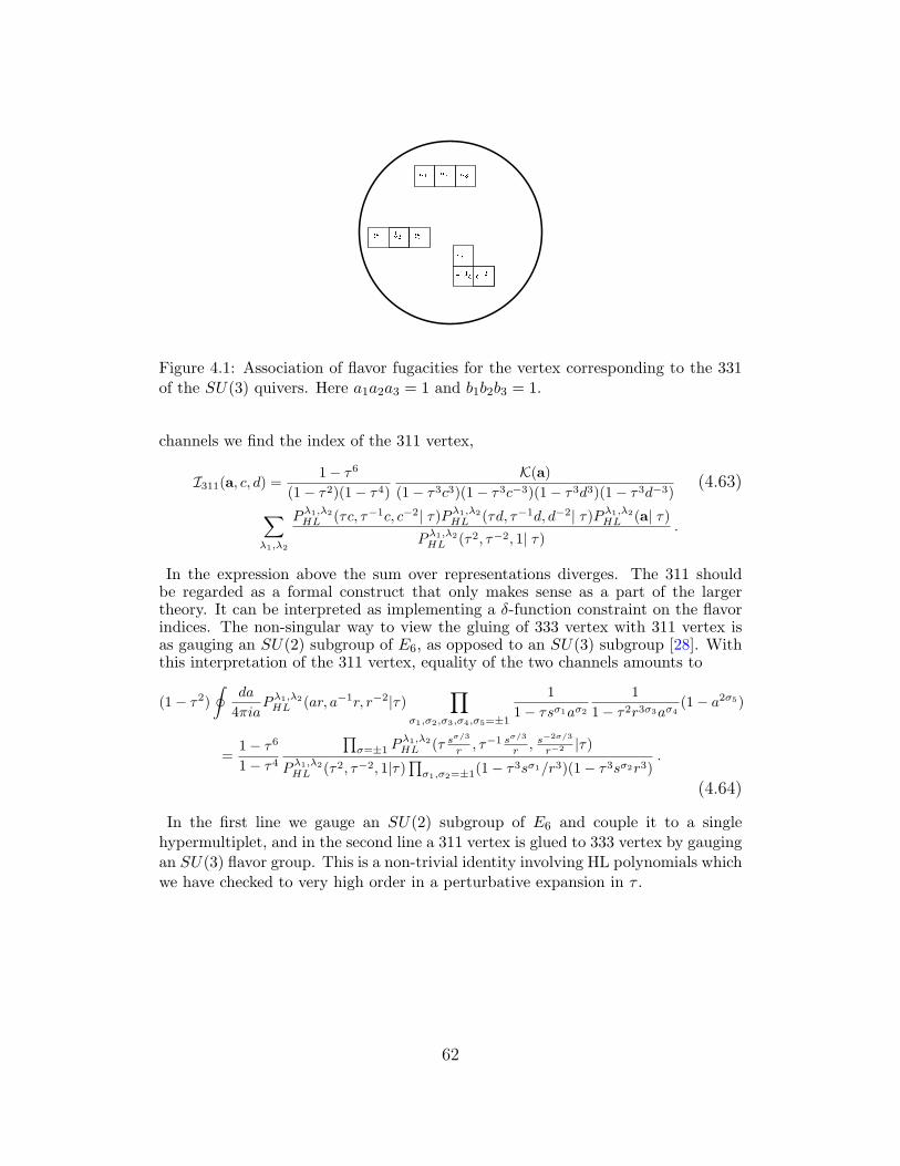
Figure 4.1: Association of flavor fugacities for the vertex corresponding to the 331of the SU(3) quivers. Here a1a2a3 = 1 and b1b2b3 = 1.
channels we find the index of the 311 vertex,
I311(a, c, d) =1− τ6
(1− τ2)(1− τ4)
K(a)
(1− τ3c3)(1− τ3c−3)(1− τ3d3)(1− τ3d−3)(4.63)
∑λ1,λ2
Pλ1,λ2
HL (τc, τ−1c, c−2| τ)Pλ1,λ2
HL (τd, τ−1d, d−2| τ)Pλ1,λ2
HL (a| τ)Pλ1,λ2
HL (τ2, τ−2, 1| τ).
In the expression above the sum over representations diverges. The 311 shouldbe regarded as a formal construct that only makes sense as a part of the largertheory. It can be interpreted as implementing a δ-function constraint on the flavorindices. The non-singular way to view the gluing of 333 vertex with 311 vertex isas gauging an SU(2) subgroup of E6, as opposed to an SU(3) subgroup [28]. Withthis interpretation of the 311 vertex, equality of the two channels amounts to
(1− τ2)
∮da
4πiaPλ1,λ2
HL (ar, a−1r, r−2|τ)∏
σ1,σ2,σ3,σ4,σ5=±1
1
1− τsσ1aσ2
1
1− τ2r3σ3aσ4(1− a2σ5)
=1− τ6
1− τ4
∏σ=±1 P
λ1,λ2
HL (τ sσ/3
r , τ−1 sσ/3
r , s−2σ/3
r−2 |τ)Pλ1,λ2
HL (τ2, τ−2, 1|τ)∏
σ1,σ2=±1(1− τ3sσ1/r3)(1− τ3sσ2r3).
(4.64)
In the first line we gauge an SU(2) subgroup of E6 and couple it to a singlehypermultiplet, and in the second line a 311 vertex is glued to 333 vertex by gaugingan SU(3) flavor group. This is a non-trivial identity involving HL polynomials whichwe have checked to very high order in a perturbative expansion in τ .
62
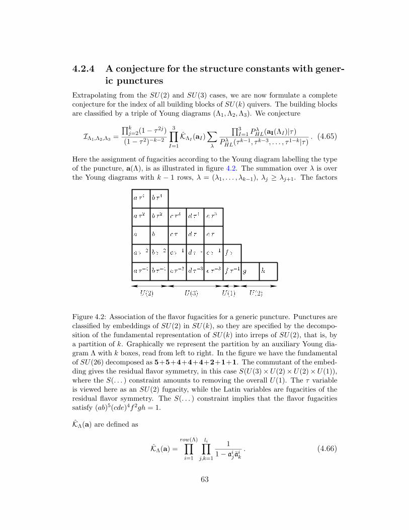
4.2.4 A conjecture for the structure constants with gener-ic punctures
Extrapolating from the SU(2) and SU(3) cases, we are now formulate a completeconjecture for the index of all building blocks of SU(k) quivers. The building blocksare classified by a triple of Young diagrams (Λ1,Λ2,Λ3). We conjecture
IΛ1,Λ2,Λ3 =
∏kj=2(1− τ2j)
(1− τ2)−k−2
3∏I=1
KΛI(aI)
∑λ
∏3I=1 P
λHL(aI(ΛI)|τ)
P λHL(τ
k−1, τk−3, . . . , τ1−k|τ). (4.65)
Here the assignment of fugacities according to the Young diagram labelling the typeof the puncture, a(Λ), is as illustrated in figure 4.2. The summation over λ is overthe Young diagrams with k − 1 rows, λ = (λ1, . . . , λk−1), λj ≥ λj+1. The factors
Figure 4.2: Association of the flavor fugacities for a generic puncture. Punctures areclassified by embeddings of SU(2) in SU(k), so they are specified by the decompo-sition of the fundamental representation of SU(k) into irreps of SU(2), that is, bya partition of k. Graphically we represent the partition by an auxiliary Young dia-gram Λ with k boxes, read from left to right. In the figure we have the fundamentalof SU(26) decomposed as 5+5+4+4+4+2+1+1. The commutant of the embed-ding gives the residual flavor symmetry, in this case S(U(3)×U(2)×U(2)×U(1)),where the S(. . . ) constraint amounts to removing the overall U(1). The τ variableis viewed here as an SU(2) fugacity, while the Latin variables are fugacities of theresidual flavor symmetry. The S(. . . ) constraint implies that the flavor fugacitiessatisfy (ab)5(cde)4f2gh = 1.
KΛ(a) are defined as
KΛ(a) =
row(Λ)∏i=1
li∏j,k=1
1
1− aij aik
. (4.66)
63
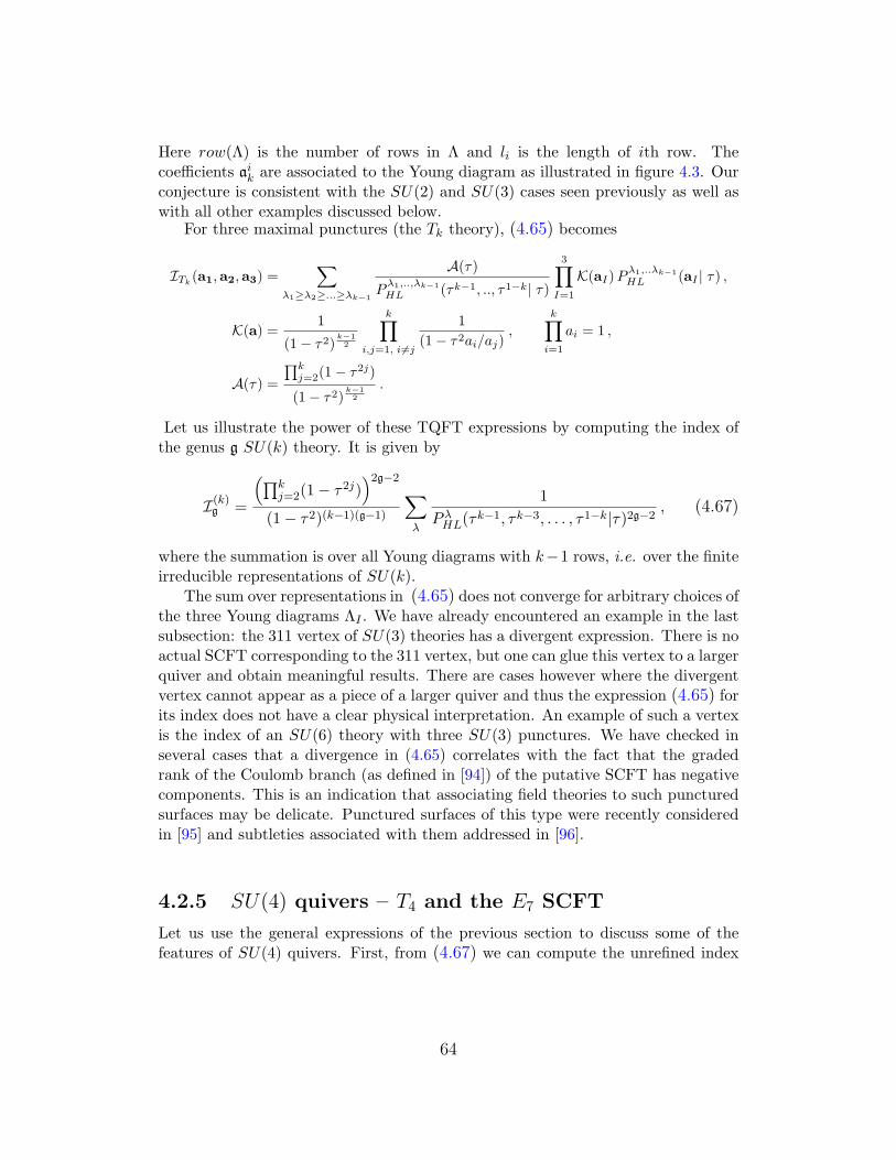
Here row(Λ) is the number of rows in Λ and li is the length of ith row. Thecoefficients aik are associated to the Young diagram as illustrated in figure 4.3. Ourconjecture is consistent with the SU(2) and SU(3) cases seen previously as well aswith all other examples discussed below.
For three maximal punctures (the Tk theory), (4.65) becomes
ITk(a1,a2,a3) =
∑λ1≥λ2≥...≥λk−1
A(τ)
Pλ1,..,λk−1
HL (τk−1, .., τ1−k| τ)
3∏I=1
K(aI)Pλ1,..λk−1
HL (aI | τ) ,
K(a) =1
(1− τ2)k−12
k∏i,j=1, i=j
1
(1− τ2ai/aj),
k∏i=1
ai = 1 ,
A(τ) =
∏kj=2(1− τ2j)
(1− τ2)k−12
.
Let us illustrate the power of these TQFT expressions by computing the index ofthe genus g SU(k) theory. It is given by
I(k)g =
(∏kj=2(1− τ2j)
)2g−2
(1− τ2)(k−1)(g−1)
∑λ
1
P λHL(τ
k−1, τk−3, . . . , τ1−k|τ)2g−2, (4.67)
where the summation is over all Young diagrams with k−1 rows, i.e. over the finiteirreducible representations of SU(k).
The sum over representations in (4.65) does not converge for arbitrary choices ofthe three Young diagrams ΛI . We have already encountered an example in the lastsubsection: the 311 vertex of SU(3) theories has a divergent expression. There is noactual SCFT corresponding to the 311 vertex, but one can glue this vertex to a largerquiver and obtain meaningful results. There are cases however where the divergentvertex cannot appear as a piece of a larger quiver and thus the expression (4.65) forits index does not have a clear physical interpretation. An example of such a vertexis the index of an SU(6) theory with three SU(3) punctures. We have checked inseveral cases that a divergence in (4.65) correlates with the fact that the gradedrank of the Coulomb branch (as defined in [94]) of the putative SCFT has negativecomponents. This is an indication that associating field theories to such puncturedsurfaces may be delicate. Punctured surfaces of this type were recently consideredin [95] and subtleties associated with them addressed in [96].
4.2.5 SU(4) quivers – T4 and the E7 SCFT
Let us use the general expressions of the previous section to discuss some of thefeatures of SU(4) quivers. First, from (4.67) we can compute the unrefined index
64
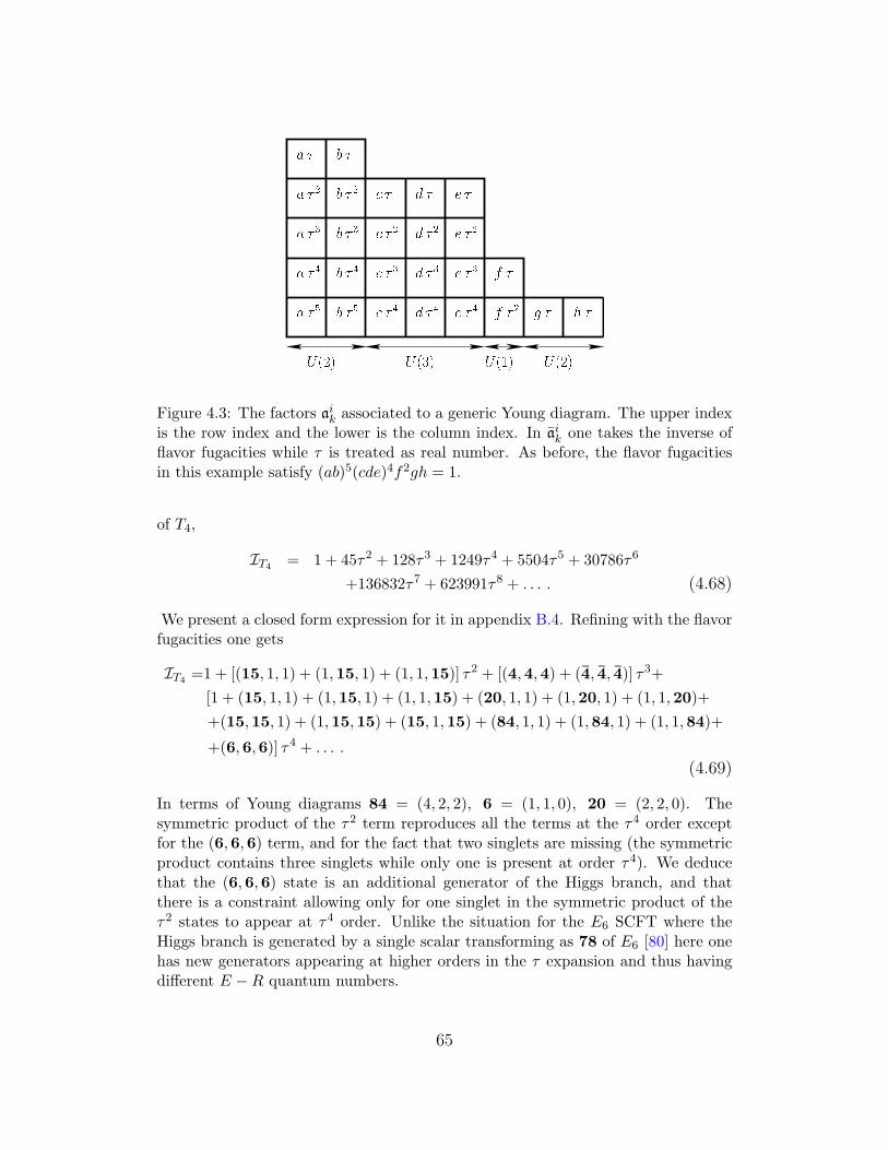
Figure 4.3: The factors aik associated to a generic Young diagram. The upper indexis the row index and the lower is the column index. In aik one takes the inverse offlavor fugacities while τ is treated as real number. As before, the flavor fugacitiesin this example satisfy (ab)5(cde)4f2gh = 1.
of T4,
IT4 = 1 + 45τ2 + 128τ3 + 1249τ4 + 5504τ5 + 30786τ6
+136832τ7 + 623991τ8 + . . . . (4.68)
We present a closed form expression for it in appendix B.4. Refining with the flavorfugacities one gets
IT4 =1 + [(15, 1, 1) + (1,15, 1) + (1, 1,15)] τ2 + [(4,4,4) + (4, 4, 4)] τ3+
[1 + (15, 1, 1) + (1,15, 1) + (1, 1,15) + (20, 1, 1) + (1,20, 1) + (1, 1,20)+
+(15,15, 1) + (1,15,15) + (15, 1,15) + (84, 1, 1) + (1,84, 1) + (1, 1,84)+
+(6,6,6)] τ4 + . . . .
(4.69)
In terms of Young diagrams 84 = (4, 2, 2), 6 = (1, 1, 0), 20 = (2, 2, 0). Thesymmetric product of the τ2 term reproduces all the terms at the τ4 order exceptfor the (6,6,6) term, and for the fact that two singlets are missing (the symmetricproduct contains three singlets while only one is present at order τ4). We deducethat the (6,6,6) state is an additional generator of the Higgs branch, and thatthere is a constraint allowing only for one singlet in the symmetric product of theτ2 states to appear at τ4 order. Unlike the situation for the E6 SCFT where theHiggs branch is generated by a single scalar transforming as 78 of E6 [80] here onehas new generators appearing at higher orders in the τ expansion and thus havingdifferent E −R quantum numbers.
65
Figure 4.4: Association of the flavor fugacities for the E7 vertex. Here∏4
i=1 bi =∏4i=1 ai = 1.
Next, we can partially close a puncture to obtain the index of the 441 vertex.On one hand, the 441 vertex correspond to the free hypermultiplet SCFT in thebifundamental of two SU(4)s and charged under the U(1), so its index can beevaluated by direct counting,
I(a1,a2, c) =4∏i,j
1
1− τaibjc
1
1− τ 1aibjc
,
4∏i=1
ai =
4∏i=1
bi = 1 . (4.70)
On the other hand, from (4.65),
I(a1,a2, c) =1− τ8
(1− τ2)
K(a1)K(a2)
(1− τ4c4)(1− τ4c−4)(4.71)
∑λ1,λ2,λ3
P λ1,λ2,λ3
HL (τ2c, c, τ−2c, c−3| τ)P λ1,λ2,λ3
HL (τ3, τ, τ−1, τ−3| τ)
2∏i=1
P λ1,λ2,λ3
HL (ai| τ) .
We have checked the equivalence of these two expressions perturbatively to veryhigh order in τ . Finally, let us look at the vertex with two maximal punctures andone puncture corresponding to a square Young diagram, which carries an SU(2)flavor symmetry, see figure 4.4. The flavor symmetry of this theory is known toenhance to E7 [28]. From (4.65), the Hall-Littlewood index of this SCFT is givenby
IE7(a1,a2, c) =(1 + τ2 + τ4)(1 + τ4)
(1− τ2)
K(a1)K(a2)
(1− τ2c±2)(1− τ4c±2)
×∑
λ1,λ2,λ3
P λ1,λ2,λ3
HL (τc, cτ ,τc ,
1τc | τ)
P λ1,λ2,λ3
HL (τ3, τ, τ−1, τ−3| τ)
2∏i=1
P λ1,λ2,λ3
HL (ai| τ) .
(4.72)
66
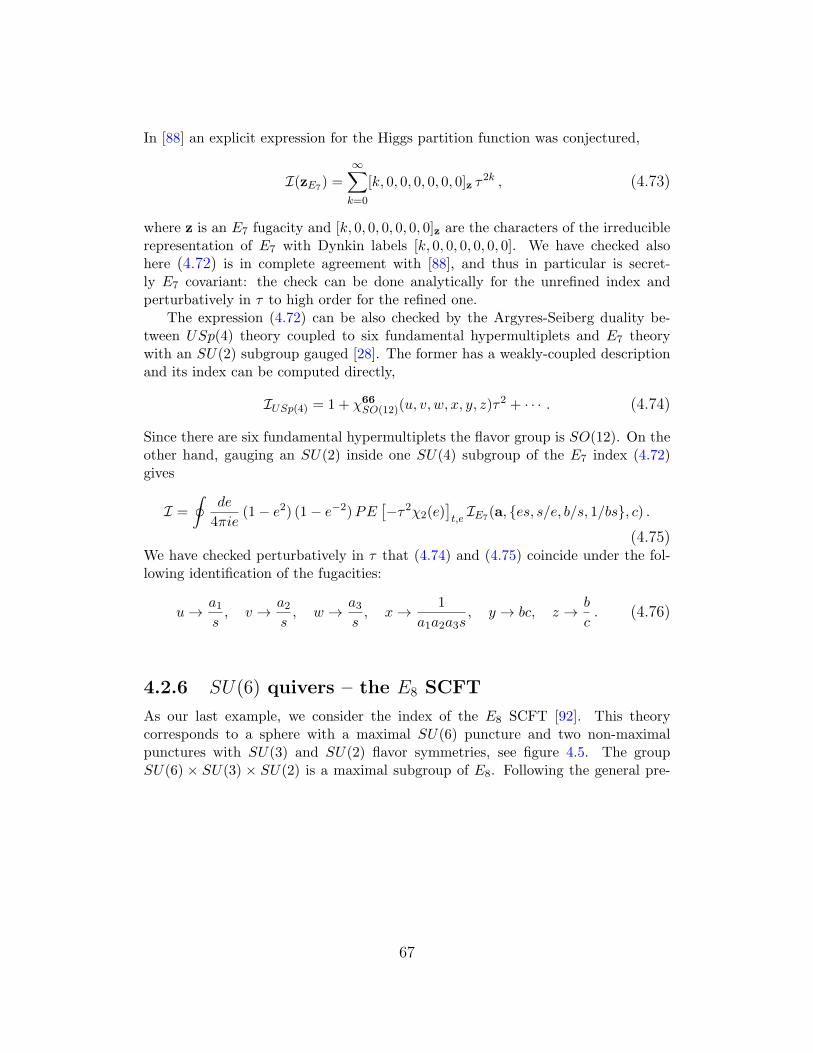
In [88] an explicit expression for the Higgs partition function was conjectured,
I(zE7) =
∞∑k=0
[k, 0, 0, 0, 0, 0, 0]z τ2k , (4.73)
where z is an E7 fugacity and [k, 0, 0, 0, 0, 0, 0]z are the characters of the irreduciblerepresentation of E7 with Dynkin labels [k, 0, 0, 0, 0, 0, 0]. We have checked alsohere (4.72) is in complete agreement with [88], and thus in particular is secret-ly E7 covariant: the check can be done analytically for the unrefined index andperturbatively in τ to high order for the refined one.
The expression (4.72) can be also checked by the Argyres-Seiberg duality be-tween USp(4) theory coupled to six fundamental hypermultiplets and E7 theorywith an SU(2) subgroup gauged [28]. The former has a weakly-coupled descriptionand its index can be computed directly,
IUSp(4) = 1 + χ66SO(12)(u, v, w, x, y, z)τ
2 + · · · . (4.74)
Since there are six fundamental hypermultiplets the flavor group is SO(12). On theother hand, gauging an SU(2) inside one SU(4) subgroup of the E7 index (4.72)gives
I =
∮de
4πie(1− e2) (1− e−2)PE
[−τ2χ2(e)
]t,e
IE7(a, es, s/e, b/s, 1/bs, c) .
(4.75)We have checked perturbatively in τ that (4.74) and (4.75) coincide under the fol-lowing identification of the fugacities:
u→ a1s, v → a2
s, w → a3
s, x→ 1
a1a2a3s, y → bc, z → b
c. (4.76)
4.2.6 SU(6) quivers – the E8 SCFT
As our last example, we consider the index of the E8 SCFT [92]. This theorycorresponds to a sphere with a maximal SU(6) puncture and two non-maximalpunctures with SU(3) and SU(2) flavor symmetries, see figure 4.5. The groupSU(6) × SU(3) × SU(2) is a maximal subgroup of E8. Following the general pre-
67
Figure 4.5: Association of the flavor fugacities for the E8 vertex. Here∏3
i=1 bi =∏6i=1 ai = 1.
scription (4.65) the index of E8 SCFT is given by
IE8(a, b1, b2, c) =(1− τ8)(1− τ10)(1− τ12)
(1− τ2)1/2(1− τ4)4(1− τ6)× (4.77)
K(a)
(1− τ2c±2)(1− τ4c±2)(1− τ6c±2)∏
i=j(1− τ2bi/bj)(1− τ4bi/bj)×
∑λ1,...,λ5≡λ
P λHL(τb1, τb2, τb3,
b1t ,
b2τ ,
b3τ | τ)P
λHL(τ
2c, c, cτ2, τ
2
c ,1c ,
1τ2c, | τ)P λ
HL(ai| τ)P λHL(τ
5, τ3, τ, τ−1, τ−3, τ−5| τ).
In [88] it was conjectured that the Higgs partition function has the following E8
covariant expansion,
I(zE8) =
∞∑k=0
[k, 0, 0, 0, 0, 0, 0, 0]z τ2k , (4.78)
where z is an E8 fugacity and [k, 0, 0, 0, 0, 0, 0, 0]z are the characters of the irreduciblerepresentation of E8 with Dynkin labels [k, 0, 0, 0, 0, 0, 0, 0]. We have again checkedequivalence of (4.77) and (4.78) in the τ -expansion, though in this case due tocomputational complexity we could perform the expansion only up to order τ8. Thesize of representations of E8 contributing to the index grows very fast with the orderof τ , e.g. the unrefined index is given by
IE8 = 1 + 245τ2 + 26255τ4 + 1681887τ6 + 73829103τ8 + . . . . (4.79)
68
4.2.7 Large k limit
It is not difficult to evaluate the large k limit of the HL index of SU(k) generalizedquivers.8 For instance, for the index of the theory corresponding to a genus g surfacewithout punctures (4.67),
I(k→∞)g =
∞∏j=2
(1− τ2j)g−1 = PE
[−(g− 1)
τ4
1− τ2
]. (4.80)
In appendix B.3 we give a short derivation of this expression. In the large k limit onlythe singlet in the sum over the representations of (4.67) contributes. Since (4.80)is of order one for large k it is expected to be matched by counting the appropriatesupergravity modes in the dual AdS background [70]. We can also compute theindex of the Tk theories in the large k limit,
ITk→∞(a1,a2,a3) =
∞∏j=2
1
1− τ2j
3∏I=1
∞∏j =i
1
1− τ2aIi /aIj
(4.81)
= PE
[τ4
1− τ2
] 3∏I=1
PE
τ2∑i=j
aIi /aIj
.From here the large k index of any generalized quiver is trivial to compute; inparticular (4.80) can be obtained by gluing together the index of (4.81). Unrefiningthe index of Tk by setting all the flavor fugacities aIj = 1 we see that it has a non-
trivial k dependence for large k limit. Taking the plethystic log of (4.81) (that is,considering the index of single-particle states) we find
Is.p.Tk→∞
= 3 τ2 (k2 − k) +τ4
1− τ2+O
(1
k
). (4.82)
The term of order k2 on the right-hand-side comes from states in the adjoint repre-sentation of the flavor group, while the term of order k comes from neutral states.At least some of O(k2) states in the adjoint representation must correspond tomodes of the AdS gauge fields that couple to the flavor currents of the boundarytheory. It would be interesting to check whether all the O(k2) and O(k) statescan be accounted for by supergravity states. If not, the extra states could arise asnon-perturbative states in the bulk geometry (e.g. wrapped branes or black holes).In all cases studied so far the index is of order one in the large k limit and thuscannot capture the non-perturbative states of the bulk theory [2, 25, 32, 97]. Thisis not a contradiction, since the index only counts protected states with signs. Theindex vanishes on combinations of short multiplets that can in principle recombine
8We thank Davide Gaiotto and Juan Maldacena for discussions on issues related to thissection.
69
into long ones, even when such kinematically-allowed recombination do not actuallyhappen [2]. However, for linear quivers (in particular for the Tk theories) the HLindex has the meaning of a Hilbert series over the Higgs branch, so it is expect-ed to capture all the relevant 3
8 -BPS states of the dual theory. We leave the veryinteresting comparison with the bulk theory for future research.
4.3 Schur index
We turn to the Schur index,
IS = Tr(−1)F qE−R , (4.83)
which is the same as the reduced index considered in [17]. Let us first recall theexpression for the SU(k) propagator. It is of the usual form
η(a,b−1) = ∆(a)IV (a)δ(a,b−1) , (4.84)
where ∆(a) is the Haar measure (4.53), and IV (a) the index of the vector multiplet,given by
IVq (a) = PE
[−2q
1− qχadj(a)
]q,a
. (4.85)
The set of functions fλq (a) that diagonalize the structure constants are propor-tional to the Schur polynomials [17],
fλq (a) = Kq(a) χλ(a) . (4.86)
The Schur polynomials are orthonormal under the Haar measure, so in this case∆(a) = ∆(a) (recall (4.10)) and the factor Kq(a) is given by
Kq(a) =1
[IVq (a)]
12
. (4.87)
Generalizing our results in [17], we conjecture the following expression for the Schurindex of a three-punctured sphere with generic punctures,
IΛ1,Λ2,Λ3 =(q; q)k+2∏k−1
j=1(1− qj)k−j
3∏I=1
KΛI(aI)
∑λ
∏3I=1 χ
λ(aI(ΛI))
χλ(qk−12 , q
k−32 , . . . , q
1−k2 )
. (4.88)
Here the sum is over the finite-dimensional irreducible representations of SU(k).The assignment of fugacities according to the Young diagram, a(Λ), is again as in
70
figure 4.2, with τ → q1/2. The Pochhammer symbol (a; b) is defined by
(a; b) =
∞∏i=0
(1− a bi) . (4.89)
The character of the representation corresponding to Young diagram λ = (λ1, . . . , λk−1, 0)is given by a Schur polynomial,
χλ(a) =det(a
λj+k−ji )
det(ak−ji )
. (4.90)
The KΛ prefactors are given by
KΛ(a) =
row(Λ)∏i=1
li∏j,k=1
PE
[aij a
ik
1− q
]ai,q
, (4.91)
where row(Λ) is the number of rows in Λ and li is the length of ith row. Thecoefficients aik are associated to the Young diagram again as in figure 4.3, withτ → q1/2. Note that the quantity appearing in the denominator of (4.88) is thequantum dimension of the representation λ of SU(k),
dimqλ = χλ(qk−12 , q
k−32 , . . . , q
1−k2 ) . (4.92)
For SU(2) the quantum dimension is also known as the q-number [λ]q.We have subjected (4.88) to similar checks as the one described for the Hall-
Littlewood index, finding complete agreement with expectations; a few such checkswere reported in [17]. Let us only mention here the basic identity following fromcompatibility of (4.88) with the index of the SU(2) trifundamental hypermultiplet,
PE
[q1/2
1− q
(a1 +
1
a1
)(a2 +
1
a2
)(a3 +
1
a3
)]ai,τ
= (4.93)
(q; q)3(q2; q)
3∏i=1
PE
[q
1− q
(a2i + a−2
i + 2)]
ai,τ
∞∑λ=0
∏3i=1 χ
λ(ai, a−1i )
χλ(q12 , q−
12 )
.
A proof of this identity is outlined in appendix B.5.
71
4.4 Macdonald index
We are now ready to combine and generalize the results of the two previous section-s. The Hall-Littlewood and Schur polynomials are special cases of a two-parameterfamily of polynomials discovered by Macdonald [93]. One naturally expects Macdon-ald polynomials to be relevant for the calculation of the index in a two-dimensionalslice of the full three-dimensional fugacity space. The precise confirmation of thisidea is our main result. Identifying the correct slice is by no means obvious, but atthis point it will come as no great surprise that it is given by the limit that we havecalled the Macdonald index in section 4.1,
IM = TrM (−1)F qE−2R−r tR+r = TrM (−1)F q−2j1 tR+r , (4.94)
where TrM denotes the trace restricted to states with δ1+ = E + 2j1 − 2R− r = 0.For q = t Macdonald polynomials reduce to Schur polynomials, while for q = 0 theyreduce to Hall-Littlewood polynomials. By design, the Macdonald trace formula(4.94) reproduces respectively the Schur and Hall-Littlewood trace formulae in thesame limits.
Our basic ansatz is that the complete set of functions fλq,t(a) that diagonalizethe structure constants are proportional to Macdonald polynomials with parametersq and t,
fλq,t(a) = Kq,t(a)Pλ(a|q, t) . (4.95)
The Macdonald polynomials [93]9 P λ(a) are defined as the set of polynomialslabeled by Young diagrams λ, orthonormal under the measure
∆q,t(a) =1
k!PE
[− 1− t
1− q(χadj(a)− k + 1)
]q,t,a
=1
k!
∞∏n=0
∏i=j
1− qnai/aj1− t qnai/aj
,(4.96)
and having the expansion
P λ = Nλ(q, t)
mλ +∑µ<λ
hλµ(q, t)mµ
. (4.97)
Here we define
mλ=(λ1,..,λk)(a) =∑σ∈S′
k
k∏i=1
aσ(λi)i , (4.98)
9Macdonald polynomials appear in physics in many different contexts. Some recentpapers on subjects related to N = 2 gauge theories that discuss Macdonald polynomialsare [98–100].
72
where S′k denotes the set of distinct permutations of (λ1, ..., λk).
The factor Kq,t(a) is again fixed by requiring orthonormality of fλq,t(a) underthe propagator measure. The propagator takes the standard form
η(a,b−1) = ∆(a)IV (a)δ(a,b−1) , (4.99)
where as always ∆(a) is the Haar measure (4.53), while the index of the vectormultiplet is in this case given by
IVq,t(a) = PE
[−q − t
1− qχadj(a)
]q,a
. (4.100)
We then have
Kq,t(a) =
(∆q,t(a)
∆(a) IVq,t(a)
) 12
. (4.101)
We can finally state our main conjecture. The Macdonald index of the SU(k)quiver theory associated to a sphere with three punctures of generic type is
IΛ1,Λ2,Λ3 = (t; q)k+2k∏
j=2
(tj ; q)
(q; q)
3∏I=1
KΛI(aI)
∑λ
∏3I=1 P
λ(aI(ΛI)|q, t)P λ(t
k−12 , t
k−32 , . . . , t
1−k2 |q, t)
.
(4.102)The assignment of fugacities according to the Young diagram ai(Λi) is again as
in figure 4.2, with τ → t1/2. The K prefactors are
KΛ(a) =
row(Λ)∏i=1
li∏j,k=1
PE
[aij a
ik
1− q
]ai,q
, (4.103)
with the coefficients aik associated to the Young diagram again as in figure 4.3,
with τ → t1/2. It is immediate to check that (4.102) reduces to the HL and Schurexpressions in the respective limits. For three maximal punctures (4.102) becomes,
ITk(a1,a2,a3) =
∑λ1≥λ2≥...≥λk−1
A(q, t)
Pλ1,..,λk−1(tk−12 , .., t
1−k2 | q, t)
3∏I=1
Kq,t(aI)Pλ1,..λk−1(aI | q, t) ,
A(q, t) =PE
[1
2(k − 1)
t− q
1− q
] k∏j=2
(tj ; q) .
(4.104)
For k = 2, this expression must agree with the index of the hypermultiplet in the
73
trifundamental representation of SU(2),
PE
[t1/2
1− q
(a1 +
1
a1
)(a2 +
1
a2
)(a3 +
1
a3
)]ai,q,t
(4.105)
=(t; q)4(t2; q)
(q; q)
3∏i=1
PE
[t
1− q
(a2i + a−2
i + 2)]
ai,q,t
∞∑λ=0
∏3i=1 P
λ(ai, a−1i |q, t)
P λ(t12 , t−
12 |q, t)
.
We have verified this identity in the t and q expansions. It helps that for SU(2) onecan write an explicit form for the Macdonald polynomials,
P λ(a, a−1|q, t) = Nλ(q, t)
λ∑i=0
i−1∏j=0
1− t qj
1− qj+1
λ−i−1∏j=0
1− t qj
1− qj+1a2i−λ , (4.106)
where Nλ(q, t) is a normalization constant rendering the Macdonald polynomialsorthonormal under the measure (4.96). More generally, equating the index for the(nn1) vertex from (4.102) with the index of a hypermultiplet in the bifundamentalrepresentation of SU(k) and charged under U(1), we obtain the identity
PE
t1/2
1− q
c k∑i,j=1
aibj +1
c
k∑i,j=1
a−1i b−1
j
a,b,c,q,t
=(t; q)k
(q; q)k−1(tk; q)
× PE
t
1− q
k∑i,j=1
ai a−1j
a,q,t
PE
t
1− q
k∑i,j=1
bi b−1j
b,q,t
PE
[tk2
1− q(ck + c−k)
]c,q,t
×∑λ
Pλ(c tk−22 , c t
k−42 , . . . , c t
2−k2 , c1−k|q, t)Pλ(ai|q, t)Pλ(bi|q, t)
Pλ(tk−12 , t
k−32 , . . . , t
1−k2 |q, t)
.
(4.107)
It would be interesting to have an analytic proof of these identities.From (4.12) we can readily calculate the index of the genus g theory with s
punctures,
Ig,s(aI ; q, t) =k∏
j=2
(tj ; q)2g−2+s (t; q)(k−1)(1−g)+s
(q; q)(k−1)(1−g)
∑λ
∏si=1 KΛi
(ai) Pλ(ai(Λi)|q, t)[
Pλ(tk−12 , t
k−32 , . . . , t
1−k2 |q, t)
]2g−2+s .
(4.108)Let us dwell upon this result. Let us first consider the genus g partition function(no punctures) in the Schur limit, q = t. We can write it as
Ig(q) =[(q; q)2g−2
]k−1S00(q)
2−2g∑λ
1
[dimq(λ)]2g−2 . (4.109)
Here S00 is the partition function of SU(k) level ℓ Chern-Simons theory on S3 if we
74
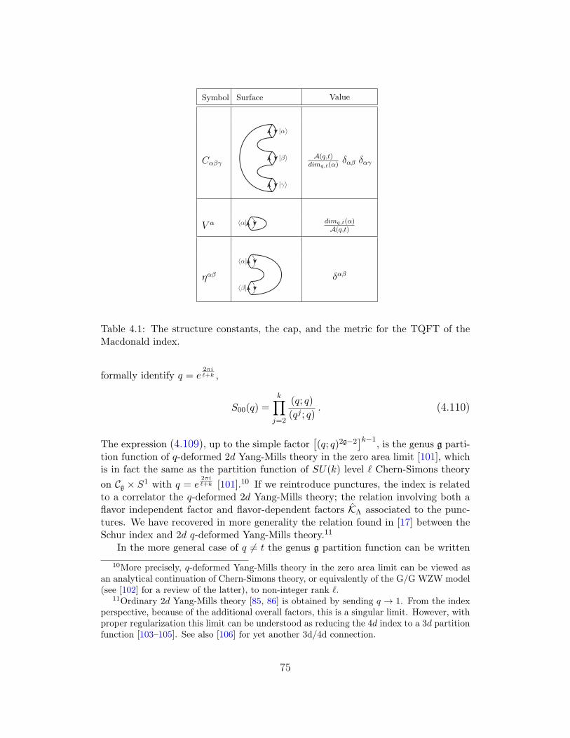
Symbol Surface Value
Cαβγ
|α〉
|β〉
|γ〉
A(q,t)dimq,t(α)
δαβ δαγ
V α 〈α| dimq,t(α)
A(q,t)
ηαβ
〈α|
〈β|
δαβ
Table 4.1: The structure constants, the cap, and the metric for the TQFT of theMacdonald index.
formally identify q = e2πiℓ+k ,
S00(q) =
k∏j=2
(q; q)
(qj ; q). (4.110)
The expression (4.109), up to the simple factor[(q; q)2g−2
]k−1, is the genus g parti-
tion function of q-deformed 2d Yang-Mills theory in the zero area limit [101], whichis in fact the same as the partition function of SU(k) level ℓ Chern-Simons theory
on Cg × S1 with q = e2πiℓ+k [101].10 If we reintroduce punctures, the index is related
to a correlator the q-deformed 2d Yang-Mills theory; the relation involving both aflavor independent factor and flavor-dependent factors KΛ associated to the punc-tures. We have recovered in more generality the relation found in [17] between theSchur index and 2d q-deformed Yang-Mills theory.11
In the more general case of q = t the genus g partition function can be written
10More precisely, q-deformed Yang-Mills theory in the zero area limit can be viewed asan analytical continuation of Chern-Simons theory, or equivalently of the G/G WZW model(see [102] for a review of the latter), to non-integer rank ℓ.
11Ordinary 2d Yang-Mills theory [85, 86] is obtained by sending q → 1. From the indexperspective, because of the additional overall factors, this is a singular limit. However, withproper regularization this limit can be understood as reducing the 4d index to a 3d partitionfunction [103–105]. See also [106] for yet another 3d/4d connection.
75
as
Ig(q, t) =[(t; q)g−1 (q; q)g−1
]k−1S00(q, t)
2−2g∑λ
1
[dimq,t(λ)]2g−2 , (4.111)
where the generalized quantum dimension is given by
dimq,t(λ) = P λ(tk−12 , t
k−32 , . . . , t
1−k2 |q, t) (4.112)
and we have defined
S00(q, t) =k∏
j=2
(t; q)
(tj ; q). (4.113)
This result appears to be closely related to the refinement of Chern-Simons the-ory recently discussed by Aganagic and Shakirov [107]. Up to the overall factor[(t; q)g−1 (q; q)g−1
]k−1, Ig(q, t) is equal to the partition function of refined Chern-
Simons on Cg × S1, and S00(q, t) to the partition function on S3. In terms of theChern-Simons matrix model the refinement of [107] amounts to changing the ma-trix integral measure from Haar to Macdonald. We can thus identify the 2d theorywhose correlators give the Macdonald index as the theory obtained from q-Yang-Mills theory by deforming in the same way the path integral measure. It would beinteresting to find a more conventional Lagrangian description of this 2d theory, forexample the deformed measure could arise by integrating out some matter fields.It would also be desirable to have a better understanding of the flavor-independentfactors needed to relate 2d Yang-Mills (q-deformed or (q, t)-deformed) to the index.They can be formally associated to a decoupled TQFT with a single operator (theidentity). Perhaps this decoupled TQFT plays a similar role as the decoupled U(1)factor in the AGT correspondence [9].
4.5 Coulomb-branch index
Finally we consider the index
ICM (T,Q) = TrCM (−1)F T12(E+2j1−2R−r)Q
12(E+2j2+2R+r) , (4.114)
where TrCM stands for the trace over states with E + 2j1 + r = 0. This limitof the full index makes sense for theories with a Lagrangian description, since thesingle-letter partition functions have well-defined expressions,
f12H = 0, fV =
T −Q
1−Q. (4.115)
76
Theories connected to Lagrangian theories by dualities also have a well-definedICM (T,Q). As discussed in section 4.1, the further limit Q→ 0 leads to the IC(T )index, which is guaranteed to be well-defined for any N = 2 SCFT.
We refer to (4.114) as the “Coulomb-branch” index, or Coulomb index for short,because in a Lagrangian theory it receives contributions only from the E-type short-multiplets (see appendix B.2), whose bottom components are the gauge-invariantoperators that parametrize the Coulomb branch, for example
Trϕ2, Trϕ3, . . . , Trϕk (4.116)
for a theory with SU(k) gauge group. Since the hypermultiplets do not contribute,the Coulomb index is independent of the flavor fugacities and the TQFT structure isvery simple. The structure constants associated to a three-punctured sphere dependonly on T and Q, and so does the propagator, since the gauge-group matrix integralcan be carried out independently of what the propagator connects to. The index ofa quiver is then just a product over the indices of its constituents (propagators andvertices).
The index of a vector multiplet in the adjoint representation of a simple gaugegroup G is
IV(G)(Q,T ) =
∮TrG
rG∏i=1
dai2πi
∆G(a) exp
[−
∞∑n=1
1
n
Qn − Tn
1−Qnχ(G)adj(a
n)
], (4.117)
where rG is the rank of G and ∆G(a) the Haar measure,
∆G(a) =1
|WG |exp
[−
∞∑n=1
1
n(χadj(a
n)− rG)
], (4.118)
with |WG | the order of the Weyl group. We recognize the integrand in (4.117) asthe Macdonald measure (4.96) with parameters Q and T . The integral can beevaluated explicitly thanks to Macdonald’s celebrated constant-term identities (seee.g. [93, 108] for pedagogic expositions and [109] for a brief review),
IVG = PE
rank(G)I1 +∑α∈R+
I1+Cα − ICα
, Cα ≡∑β∈R+
(α, β)
(β, β),(4.119)
where R+ is the collection of positive roots of G and
Iℓ = T ℓ−1T −Q
1−Q. (4.120)
We recognize Iℓ as the index of the E−ℓ(0,0) superconformal multiplet, which satisfiesthe shortening condition E = ℓ (see appendix B.2). By a Lie-algebraic identity,
77
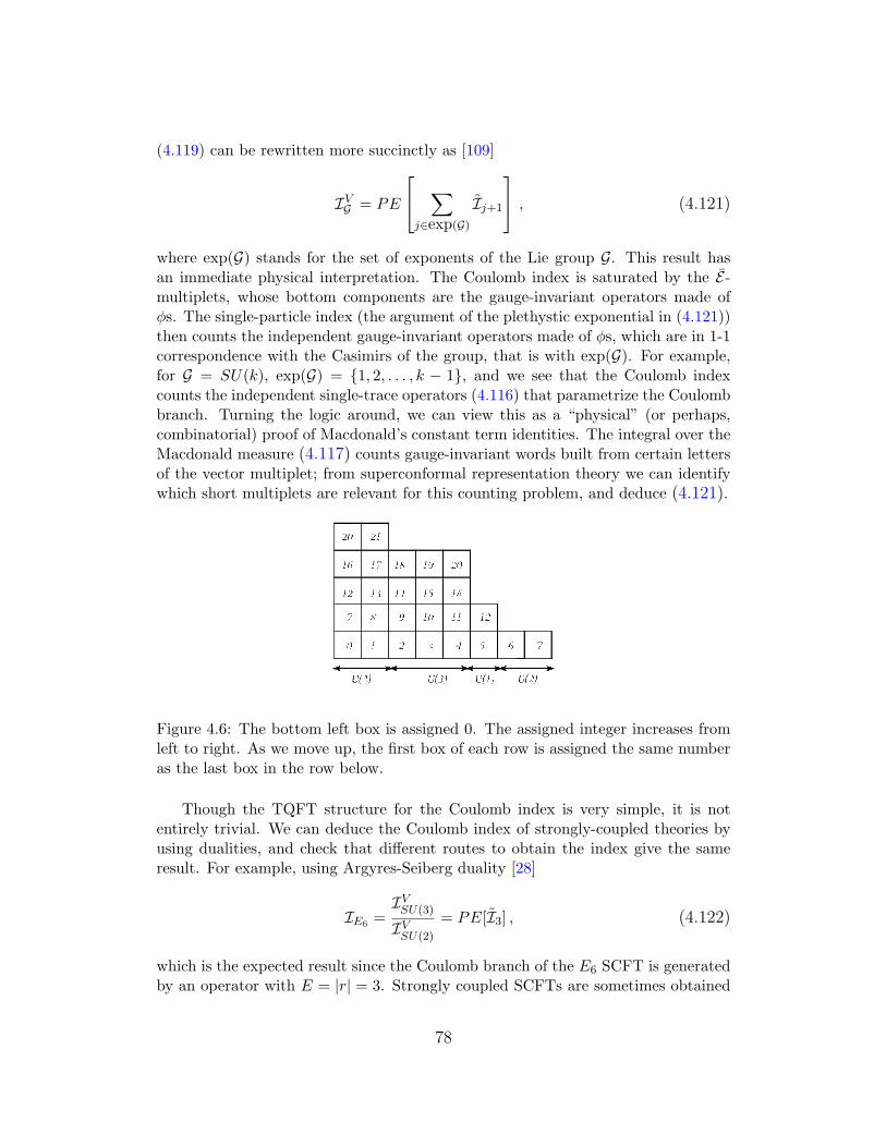
(4.119) can be rewritten more succinctly as [109]
IVG = PE
∑j∈exp(G)
Ij+1
, (4.121)
where exp(G) stands for the set of exponents of the Lie group G. This result hasan immediate physical interpretation. The Coulomb index is saturated by the E-multiplets, whose bottom components are the gauge-invariant operators made ofϕs. The single-particle index (the argument of the plethystic exponential in (4.121))then counts the independent gauge-invariant operators made of ϕs, which are in 1-1correspondence with the Casimirs of the group, that is with exp(G). For example,for G = SU(k), exp(G) = 1, 2, . . . , k − 1, and we see that the Coulomb indexcounts the independent single-trace operators (4.116) that parametrize the Coulombbranch. Turning the logic around, we can view this as a “physical” (or perhaps,combinatorial) proof of Macdonald’s constant term identities. The integral over theMacdonald measure (4.117) counts gauge-invariant words built from certain lettersof the vector multiplet; from superconformal representation theory we can identifywhich short multiplets are relevant for this counting problem, and deduce (4.121).
Figure 4.6: The bottom left box is assigned 0. The assigned integer increases fromleft to right. As we move up, the first box of each row is assigned the same numberas the last box in the row below.
Though the TQFT structure for the Coulomb index is very simple, it is notentirely trivial. We can deduce the Coulomb index of strongly-coupled theories byusing dualities, and check that different routes to obtain the index give the sameresult. For example, using Argyres-Seiberg duality [28]
IE6 =IVSU(3)
IVSU(2)
= PE[I3] , (4.122)
which is the expected result since the Coulomb branch of the E6 SCFT is generatedby an operator with E = |r| = 3. Strongly coupled SCFTs are sometimes obtained
78
using S-dualities in more than one way [77] but all the dualities yield the same index,for example
IE6 =IVSU(3)
IVSU(2)
=IVSU(4)
IVUSp(4)
= PE[I3] ,
IE7 =IVSU(4)
IVSU(3)
=IVUSp(4)
IVSU(2)
=IVSO(7)
IVG2
=IVSO(8)
IVSO(7)
= PE[I4] , (4.123)
IE8 =IVSU(6)
IVSU(5)
=IVUSp(6)
IVSO(5)
= PE[I6] .
The index of the Tk theory is also obtained easily from the generalized Argyres-Seiberg duality,
ITk=
(IVSU(k))
k−2∏k−1j=2 IV
SU(j)
= PE
k∑j=3
(j − 2)Ij
. (4.124)
This is again as expected, since the Coulomb branch of the Tk theory is spanned by(j − 2) operators with E = |r| = j, for j = 3, . . . , k (see e.g. [73]).
Extrapolating from these examples let us conjecture the Coulomb index of thetheory corresponding to a sphere with three generic punctures. For a general punc-
ture I in the Ak−1 theory, we associate the set of k numbers p(I)j : j = 1, . . . kfrom the corresponding auxiliary Young diagram. The assignment is illustrated infigure 4.6. The Coulomb branch index of the theory corresponding to a sphere withthree punctures p(1), p(2), p(3) is then
Ip(1),p(2),p(3) = PE[dj Ij
], dj ≡
k∑j=2
(1− 2j + p(1)j + p
(2)j + p
(3)j ) . (4.125)
The dimension dj of the Coulomb branch spanned by operators with E = |r| = j a-grees with the dimension of the space of meromorphic j-differentials on the Riemann
surface having poles of order at most p(I)j at puncture I [3, 94].
Let us finally observe that the Coulomb index (4.117) discussed in this sectioncan also be interpreted as the index of N = 4 SYM in a certain limit of the N = 4superconformal fugacities, such that the index of the N = 4 vector multiplet reducesto the index of N = 2 vector multiplet. The authors of [110] noticed the appearanceof the Macdonald measure in this context.
79
Chapter 5
Reducing the 4d Index to the S3
Partition Function
String/M theory has led to a rich web of non-perturbative dualities between su-persymmetric field theories. Checking/exploiting/extending these dualities requiresexact computations in field theories. In recent years, using methods based on local-ization, several exact quantities in supersymmetric gauge theories have been com-puted. The connection between two of such quantities, the superconformal index of4d gauge theories [2, 14] and the partition function of supersymmetric gauge theorieson S3 [33, 40], is the main focus of this chapter.
The superconformal index of N = 1 IR fixed points was first computed in [21–23], there it served as a check of Seiberg duality. The indices ofN = 4 SYM and typeIIB supergravity in AdS5 were computed and matched in [2]. The superconformalindex of N = 2 supersymmetric gauge theories was used to check N = 2 S-dualitiesconjectured by Gaiotto and to define a 2d topological field theory in the processas discussed in chapter 3 and 4. Recently the partition function of supersymmetricgauge theories on S3 has been used to check a variety of 3d dualities includingmirror symmetry [33] and Seiberg-like dualities [34]. Remarkably, the exact partitionfunction has also allowed for a direct field theory computation of N3/2 degrees offreedom of ABJM theory [35, 36]. The S3 partition function of N = 2 theoriesis extremized by the exact superconformal R-symmetry [37–39] so just like the a-maximization in 4d, the 3d partition function can be used to determine the exactR-charges at interacting fixed points. The purpose of this chapter is to relate thesetwo interesting and useful exactly calculable quantities in 3 and 4 dimensions.
As mentioned in section 2.5 the superconformal index of a 4d gauge theory canbe computed as a path integral on S3×S1 with supersymmetric boundary conditionsalong S1 (2.49). All the modes on the S1 contribute to this path integral. In a limitwith the radius of the circle shrinking to zero the higher modes become very heavyand decouple. The index is then given by a path integral over just the constantmodes on the circle. In other words, the superconformal index of the 4d theory
80
reduces to a partition function of the dimensionally reduced 3d gauge theory onS3. The 3d theory preserves all the supersymmetries of the “parent” 4d theory onS3 × S1.
More generally, for any d dimensional manifold Md, one would expect the indexof a supersymmetric theory on Md×S1 to reduce to the exact partition function ofdimensionally reduced theory on Md. This idea was applied by Nekrasov to obtainthe partition function of 4d gauge theory on Ω-deformed background as a limit ofthe index of a 5d gauge theory [12].
A crucial property of the four dimensional index that facilitates its computationis the fact that it can be computed exactly by a saddle point integral. We showthat in the limit of vanishing circle radius, this matrix integral reduces to the onethat computes the partition function of 3d gauge theories on S3 [33, 40]. It doesn’tcome as a surprise as the path integral of the N = 2 supersymmetric gauge theoryon S3 was also shown to localize on saddle points of the action.
The chapter is organized a follows. We have already written the superconformalindex of 4d theory as a saddle point integral and describe the limit in which thisintegral reduces to the S3 partition function in section 2.5. The limit is performedin section 5.1. In particular, we show that the building blocks of the matrix mod-el that computes the superconformal index in 4d map separately to the buildingblocks of the 3d partition function matrix model. In section 5.2, we comment onthe connections between 4d and 3d dualities. We conclude with an appendix thatgeneralizes the Kapustin et. al. matrix model for N = 4 gauge theories with twosupersymmetric deformations. One such deformation involving squashed S3 wasstudied in [57]. Discussion of the similar material can also be found in [103, 105].
5.1 4d Index to 3d Partition function on S3
A matrix model for computing the partition function of 3d gauge theories on S3 (S3
matrix model) was obtained in [33, 40]. In this section, we will derive this matrixmodel as a β → 0 limit of the matrix model that computes the superconformalindex (2.52) (index matrix model) of the 4d gauge theories. Both matrix modelsinvolve integrals over gauge group parameters and their integrand contains one-loopcontributions from vector- and hyper-multiplets. We will show that the gauge groupintegral together with the contribution from the vector multiplet map nicely fromthe index model to the S3 model. The contributions of the hypermultiplets matchup separately. We also show that the superconformal index is the q-deformation ofthe S3 partition function of the daughter theory.
5.1.1 Building blocks of the matrix models
For concreteness, let us consider 4d N = 2 SU(N) gauge theory. It is constructedusing two basic building blocks: hyper-multiplets and vector multiplets.
81

Hyper-multiplet
As was first observed in [21], the index of the hypermultiplet can be written elegantlyin terms of a special function [15]
Ihyp =∏i
Γ
(t2√vai; t
3y, t3y−1
), (5.1)
where Γ is the elliptic gamma function [111] defined to be
Γ(z; r, s) =∏j,k≥0
1− z−1rj+1sk+1
1− zrjsk, (5.2)
and ai are eigenvalues of the maximal torus of the gauge/flavor group satisfying∏Ni=1 ai = 1. In this section, for the sake of simplicity, we set v = t and y = 1 and
will discuss the general assignment of chemical potentials in appendix C. We choosea convenient variable q ≡ e−β to parametrize the chemical potentials of the Cartanof the flavor group as ai = q−iαi , and the chemical potential t as t = q
13 . The index
of the hyper-multiplet then becomes
Ihyp =∏i
∏j,k≥0
1− q−12+iαiqj+1qk+1
1− q12−iαiqjqk
=∏i
∏n≥1
([n+ 1
2 + iαi]q
[n− 12 − iαi]q
)n
, (5.3)
where [n]q ≡ 1−qn
1−q is the q-number. It has the property [n]qq→1−→ n. So far we have
fixed the chemical potentials v and y that couple to −(R + r) and j1 respectively.To recover 3d partition function on S3 we should take the radius of S1 to be verysmall, which corresponds to the limit q → 1.
Ihyp =∏i
∏n≥1
(n+ 1
2 + iαi
n− 12 − iαi
)n
=∏i
(coshπαi)− 1
2 . (5.4)
One can find a proof of the second equality in [40]. From the limiting procedure, itis clear that the superconformal index of the hypermultiplet is the q-deformation ofthe 3d hypermultiplet partition function.
Vector multiplet
The index of an N = 2 vector multiplet is given by
Ivector =∏i<j
1
(1− ai/aj)(1− aj/ai)
Γ(t2v(ai/aj)±; t3y, t3y−1)
Γ((ai/aj)±; t3y, t3y−1), (5.5)
Here we have dropped an overall ai-independent factor. We use the condensednotation, Γ(z±1; r, s) = Γ(z−1; r, s)Γ(z; r, s). With the same variable change as
82
above we get
Ivector =∏i<j
1
1− qi(αi−αj)
1
1− q−i(αi−αj)
1
Γ(q±i(αi−αj); q, q)
=∏i<j
1
1− qi(αi−αj)
1
1− q−i(αi−αj)
∏n≥1
(1− qn+i(αi−αj)+1
1− qn−i(αi−αj)−1
1− qn−i(αi−αj)+1
1− qn+i(αi−αj)−1
)−n
reg=
∏i<j
∏n≥1
([n− i(αi − αj)]q
[n]q
[n+ i(αi − αj)]q[n]q
)2
.
(5.6)
The last line involves regulating the infinite product in a way that doesn’t dependon α. In the limit q → 1, i.e. the radius of the circle goes to zero, we get
Ivector =∏i<j
∏n≥1
(1 +
(αi − αj)2
n2
)2
=∏i<j
(sinhπ(αi − αj)
π(αi − αj)
)2
. (5.7)
The last equality again is explained in [40]. Again, the we see that the index ofthe vector multiplet is the q-deformation of the 3d vector partition function. Mostgeneral expression for the one-loop contribution of the vector multiplet with u andη turned on is obtained in appendix C.
Gauge group integral
The gauge group integral in the 4d index matrix model is done with the invariantHaar measure
[dU ] =∏i
dαi
∏i<j
sin2(β(αi − αj)
2
)β→0−→
∏i
dαi
∏i<j
(β(αi − αj)
2
)2
. (5.8)
After appropriate regularization, the measure factor precisely cancels the weightfactor in the denominator of the vector multiplet one-loop determinant. The unitarygauge group integral in the index matrix model can be done as a contour integralover a variables parametrizing the Cartan sub-group, i.e. a ∈ T. After the changevariables a = q−iα the contour integral becomes a line integral as follows. We writea = q−iα = eiβα. The contour integral around the unit circle is then∮
T
da
a· · · =
∫ π/β
−π/βdα . . . : β → 0,
∮T
da
a· · · =
∫ ∞
−∞dα . . . . (5.9)
83
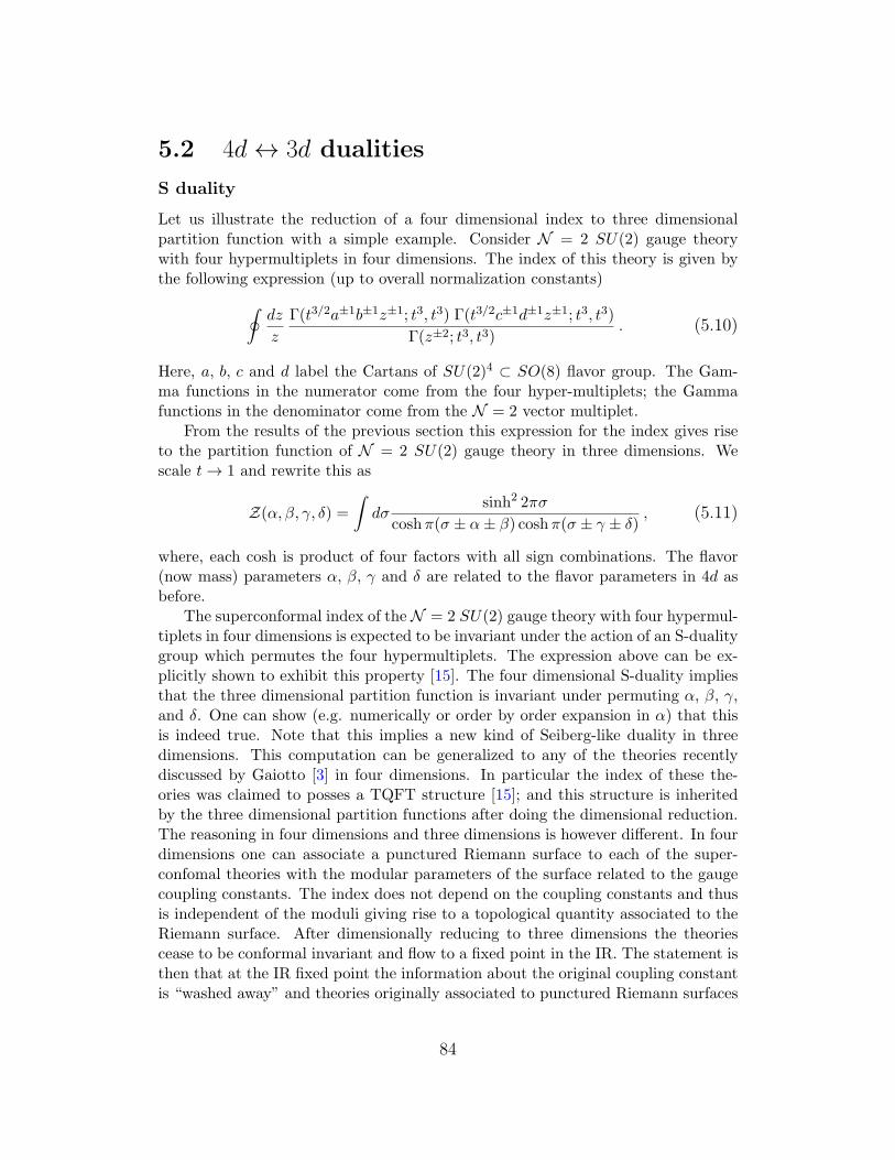
5.2 4d↔ 3d dualities
S duality
Let us illustrate the reduction of a four dimensional index to three dimensionalpartition function with a simple example. Consider N = 2 SU(2) gauge theorywith four hypermultiplets in four dimensions. The index of this theory is given bythe following expression (up to overall normalization constants)∮
dz
z
Γ(t3/2a±1b±1z±1; t3, t3) Γ(t3/2c±1d±1z±1; t3, t3)
Γ(z±2; t3, t3). (5.10)
Here, a, b, c and d label the Cartans of SU(2)4 ⊂ SO(8) flavor group. The Gam-ma functions in the numerator come from the four hyper-multiplets; the Gammafunctions in the denominator come from the N = 2 vector multiplet.
From the results of the previous section this expression for the index gives riseto the partition function of N = 2 SU(2) gauge theory in three dimensions. Wescale t→ 1 and rewrite this as
Z(α, β, γ, δ) =
∫dσ
sinh2 2πσ
coshπ(σ ± α± β) coshπ(σ ± γ ± δ), (5.11)
where, each cosh is product of four factors with all sign combinations. The flavor(now mass) parameters α, β, γ and δ are related to the flavor parameters in 4d asbefore.
The superconformal index of the N = 2 SU(2) gauge theory with four hypermul-tiplets in four dimensions is expected to be invariant under the action of an S-dualitygroup which permutes the four hypermultiplets. The expression above can be ex-plicitly shown to exhibit this property [15]. The four dimensional S-duality impliesthat the three dimensional partition function is invariant under permuting α, β, γ,and δ. One can show (e.g. numerically or order by order expansion in α) that thisis indeed true. Note that this implies a new kind of Seiberg-like duality in threedimensions. This computation can be generalized to any of the theories recentlydiscussed by Gaiotto [3] in four dimensions. In particular the index of these the-ories was claimed to posses a TQFT structure [15]; and this structure is inheritedby the three dimensional partition functions after doing the dimensional reduction.The reasoning in four dimensions and three dimensions is however different. In fourdimensions one can associate a punctured Riemann surface to each of the super-confomal theories with the modular parameters of the surface related to the gaugecoupling constants. The index does not depend on the coupling constants and thusis independent of the moduli giving rise to a topological quantity associated to theRiemann surface. After dimensionally reducing to three dimensions the theoriescease to be conformal invariant and flow to a fixed point in the IR. The statement isthen that at the IR fixed point the information about the original coupling constantis “washed away” and theories originally associated to punctured Riemann surfaces
84
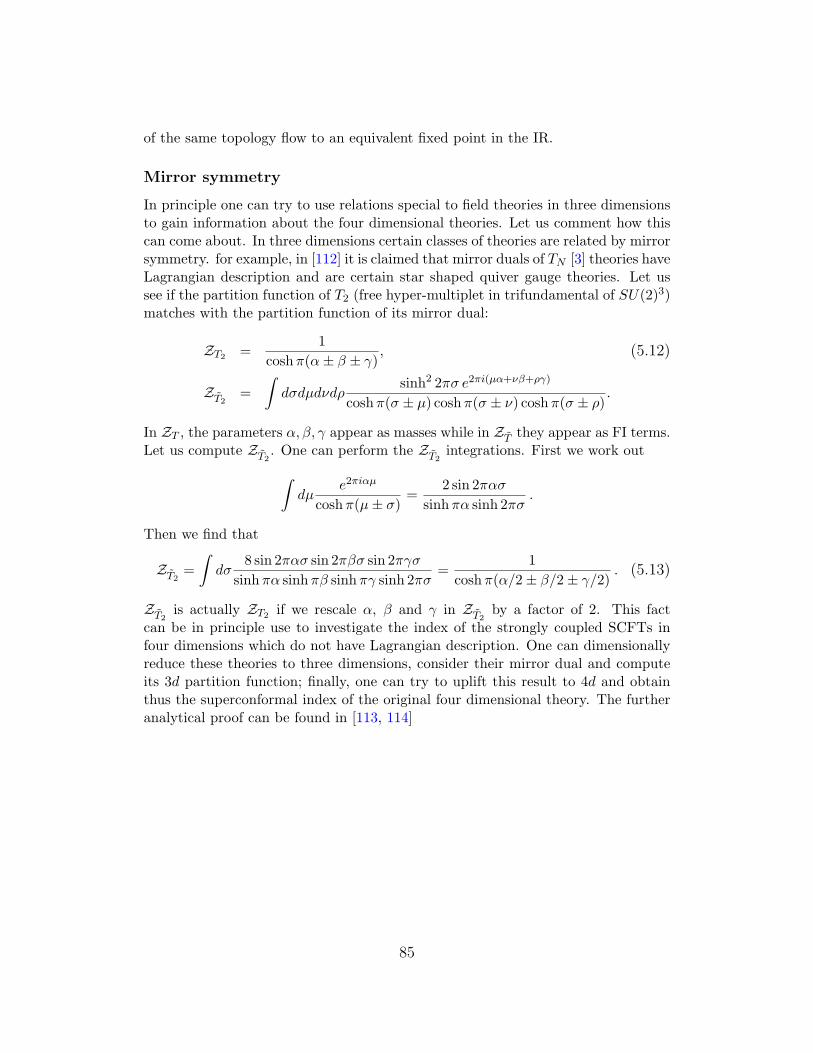
of the same topology flow to an equivalent fixed point in the IR.
Mirror symmetry
In principle one can try to use relations special to field theories in three dimensionsto gain information about the four dimensional theories. Let us comment how thiscan come about. In three dimensions certain classes of theories are related by mirrorsymmetry. for example, in [112] it is claimed that mirror duals of TN [3] theories haveLagrangian description and are certain star shaped quiver gauge theories. Let ussee if the partition function of T2 (free hyper-multiplet in trifundamental of SU(2)3)matches with the partition function of its mirror dual:
ZT2 =1
coshπ(α± β ± γ), (5.12)
ZT2=
∫dσdµdνdρ
sinh2 2πσ e2πi(µα+νβ+ργ)
coshπ(σ ± µ) coshπ(σ ± ν) coshπ(σ ± ρ).
In ZT , the parameters α, β, γ appear as masses while in ZT they appear as FI terms.Let us compute ZT2
. One can perform the ZT2integrations. First we work out∫
dµe2πiαµ
coshπ(µ± σ)=
2 sin 2πασ
sinhπα sinh 2πσ.
Then we find that
ZT2=
∫dσ
8 sin 2πασ sin 2πβσ sin 2πγσ
sinhπα sinhπβ sinhπγ sinh 2πσ=
1
coshπ(α/2± β/2± γ/2). (5.13)
ZT2is actually ZT2 if we rescale α, β and γ in ZT2
by a factor of 2. This factcan be in principle use to investigate the index of the strongly coupled SCFTs infour dimensions which do not have Lagrangian description. One can dimensionallyreduce these theories to three dimensions, consider their mirror dual and computeits 3d partition function; finally, one can try to uplift this result to 4d and obtainthus the superconformal index of the original four dimensional theory. The furtheranalytical proof can be found in [113, 114]
85
Chapter 6
The Superconformal Index ofN = 1 IR Fixed Points
In section 2.2 we review the Romelsberger prescription [14, 19] to evaluate the indexof such SCFTs the N = 1 SCFTs that arise as IR fixed points of renormalizationgroup flows, whose UV starting points are weakly-coupled theories. This prescrip-tion has so far been checked indirectly, by showing in several examples that it givesthe same result for different RG flows that end in the same IR fixed point (i.e.the UV theories are Seiberg dual). This was originally observed by Romelsberger,who performed a few perturbative checks in a chemical potential expansion [14, 19].Invariance of the N = 1 index under Seiberg duality was systematically demonstrat-ed by Dolan and Osborn [21], in a remarkable paper that first applied the elliptichypergeometric machinery to the evaluation of the superconformal index. Theseresults were extended and generalized in [22–24, 26].
In this chapter we apply Romelsberger’s prescription to a class of N = 1 SCFTsthat admit AdS duals. The canonical example is the conifold theory of Klebanov andWitten [30]. There are infinitely many generalizations: the families of toric quiversY p,q [1] and Lp,q,r [31]. We focus on Y p,q. In all these examples there is in principlean independent way to determine the index (at large N) from the dual supergravity.We will explicitly show agreement between the gravity calculation of Nakayama [32]and our field theory calculation for the case of the conifold quiver Y 1,0. Accordingto taste, this can be viewed either as a check of Romelsberger’s prescription, or asyet another check of AdS/CFT. The upshot is a sharper bulk/boundary dictionary.
In section 6.1 we review basic facts about the Y p,q family of toric quivers (theconifold being a special case Y 1,0). From the quiver diagrams, it is immediate towrite integral expressions for the superconformal index, at finite N . We show thatthe indices of toric-dual theories are equal, as expected. In section 6.2 we consid-er the large N limit. We conjecture a simple closed form expression for the largeN index of the Y p,q quivers. In section 6.3 we review the gravity computation ofthe index for the conifold [32] and find exact agreement with the large N limit of
86
our field theory result. appendix D collects useful material about N = 1 super-conformal representation theory and the index of the different short and semishortsupermultiplets.
6.1 The Y p,q quiver gauge theories
Let us begin by recalling the basic facts about the Y p,q quiver gauge theories [1].The fields are of four types: Uα=1,2, Vα=1,2, Y and Z. There are 2p gauge groups,and 4p+ 2q bifundamental fields: p fields of type U , q fields of type V , p− q fieldsof type Z, and p + q fields of type Y . The Y p,q quiver diagram is obtained by arecursive procedure starting with Y p,p, which is a familiar Z2p orbifold of N = 4SYM. The superpotential takes the form
W =∑
ϵαβTr(Ukα V
kβ Y
2k+2 + V kα U
k+1β Y 2k+3
)+ ϵαβ
∑Tr(Zk Uk+1
α Y 2k+3 Ukβ
),
where the cubic and quartic gauge-invariant terms are read off from the quiverdiagram. There are 2q terms in the first sum and p − q terms in the second sum.For the Klebanov-Witten theory, T 1,1 = Y 1,0 has only quartic terms.
The R-charges are determined as follows [1, 115]. Requiring the vanishing of theNSVZ beta functions and that each term of the superpotential has R-charge 2, theR-charges of all the fields are fixed in terms of two independent parameters x andy,
rZk = x, rY k = y, rUkα= 1− 1
2(x+ y), rV k
α= 1 +
1
2(x− y) . (6.1)
This twofold ambiguity is related to the existence of two U(1) global symmetries,and is resolved by a-maximization. One finds [1]
yp,q =1
3q2
−4p2 + 2pq + 3q2 + (2p− q)
√4p2 − 3q2
, (6.2)
xp,q =1
3q2
−4p2 − 2pq + 3q2 + (2p+ q)
√4p2 − 3q2
.
For any p, there are simple special cases. The Y p,p quiver corresponds to the Z2p
orbifold of C3. In this case all the superpotential terms are cubic, the theory isexactly conformal and all R-charges are equal to 2
3 . This theory has N = 1 super-symmetry for general p while for p = 1 the supersymmetry is enhanced to N = 2.At the other extreme, the Y p,0 quiver corresponds to a Zp orbifold of the conifold.All the R-charges are equal to 1
2 and the superpotential is quartic. The associatedquiver diagrams for p = 4 are shown in figure 6.1.
The charges of the fields under the global symmetries U(1)B, U(1)s and SU(2)l
87
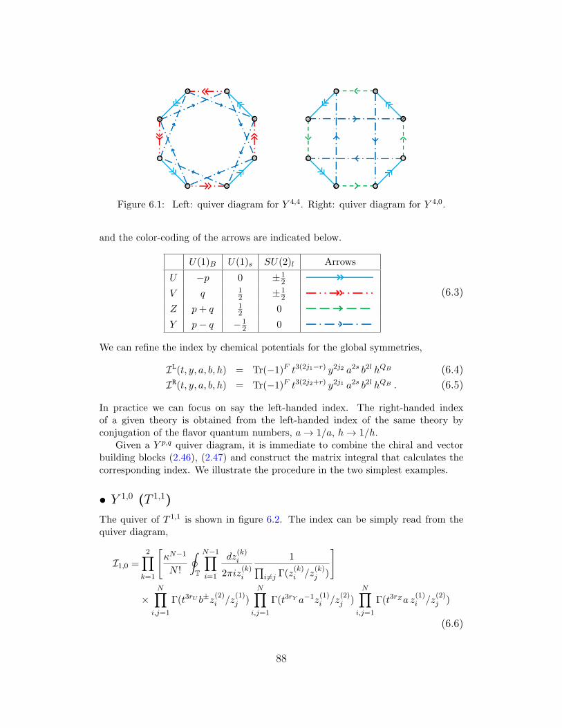
Figure 6.1: Left: quiver diagram for Y 4,4. Right: quiver diagram for Y 4,0.
and the color-coding of the arrows are indicated below.
U(1)B U(1)s SU(2)l Arrows
U −p 0 ±12
V q 12 ±1
2
Z p+ q 12 0
Y p− q −12 0
(6.3)
We can refine the index by chemical potentials for the global symmetries,
IL(t, y, a, b, h) = Tr(−1)F t3(2j1−r) y2j2 a2s b2l hQB (6.4)
IR(t, y, a, b, h) = Tr(−1)F t3(2j2+r) y2j1 a2s b2l hQB . (6.5)
In practice we can focus on say the left-handed index. The right-handed indexof a given theory is obtained from the left-handed index of the same theory byconjugation of the flavor quantum numbers, a→ 1/a, h→ 1/h.
Given a Y p,q quiver diagram, it is immediate to combine the chiral and vectorbuilding blocks (2.46), (2.47) and construct the matrix integral that calculates thecorresponding index. We illustrate the procedure in the two simplest examples.
• Y 1,0 (T 1,1)
The quiver of T 1,1 is shown in figure 6.2. The index can be simply read from thequiver diagram,
I1,0 =2∏
k=1
[κN−1
N !
∮T
N−1∏i=1
dz(k)i
2πiz(k)i
1∏i=j Γ(z
(k)i /z
(k)j )
]
×N∏
i,j=1
Γ(t3rU b±z(2)i /z
(1)j )
N∏i,j=1
Γ(t3rY a−1z(1)i /z
(2)j )
N∏i,j=1
Γ(t3rZa z(1)i /z
(2)j )
(6.6)
88
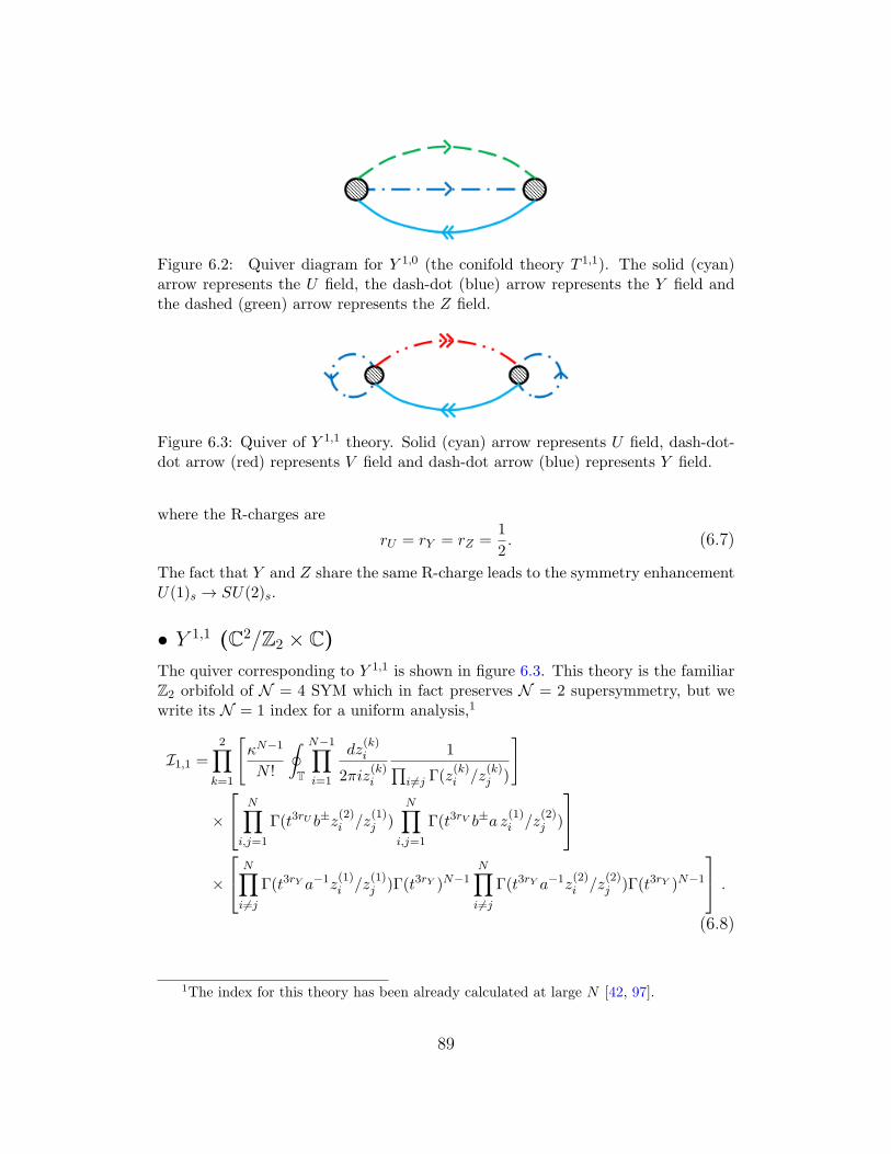
Figure 6.2: Quiver diagram for Y 1,0 (the conifold theory T 1,1). The solid (cyan)arrow represents the U field, the dash-dot (blue) arrow represents the Y field andthe dashed (green) arrow represents the Z field.
Figure 6.3: Quiver of Y 1,1 theory. Solid (cyan) arrow represents U field, dash-dot-dot arrow (red) represents V field and dash-dot arrow (blue) represents Y field.
where the R-charges are
rU = rY = rZ =1
2. (6.7)
The fact that Y and Z share the same R-charge leads to the symmetry enhancementU(1)s → SU(2)s.
• Y 1,1 (C2/Z2 × C)The quiver corresponding to Y 1,1 is shown in figure 6.3. This theory is the familiarZ2 orbifold of N = 4 SYM which in fact preserves N = 2 supersymmetry, but wewrite its N = 1 index for a uniform analysis,1
I1,1 =2∏
k=1
[κN−1
N !
∮T
N−1∏i=1
dz(k)i
2πiz(k)i
1∏i=j Γ(z
(k)i /z
(k)j )
]
×
N∏i,j=1
Γ(t3rU b±z(2)i /z
(1)j )
N∏i,j=1
Γ(t3rV b±a z(1)i /z
(2)j )
×
N∏i=j
Γ(t3rY a−1z(1)i /z
(1)j )Γ(t3rY )N−1
N∏i =j
Γ(t3rY a−1z(2)i /z
(2)j )Γ(t3rY )N−1
.(6.8)
1The index for this theory has been already calculated at large N [42, 97].
89
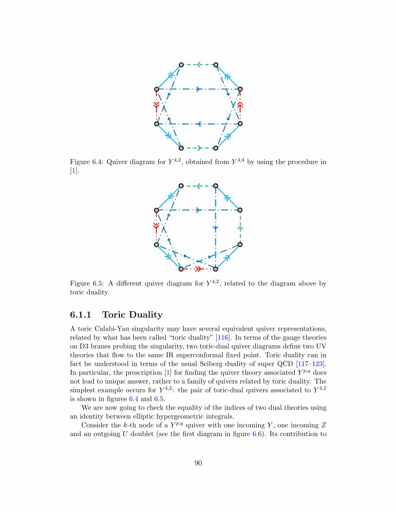
Figure 6.4: Quiver diagram for Y 4,2, obtained from Y 4,4 by using the procedure in[1].
Figure 6.5: A different quiver diagram for Y 4,2, related to the diagram above bytoric duality.
6.1.1 Toric Duality
A toric Calabi-Yau singularity may have several equivalent quiver representations,related by what has been called “toric duality” [116]. In terms of the gauge theorieson D3 branes probing the singularity, two toric-dual quiver diagrams define two UVtheories that flow to the same IR superconformal fixed point. Toric duality can infact be understood in terms of the usual Seiberg duality of super QCD [117–123].In particular, the prescription [1] for finding the quiver theory associated Y p,q doesnot lead to unique answer, rather to a family of quivers related by toric duality. Thesimplest example occurs for Y 4,2: the pair of toric-dual quivers associated to Y 4,2
is shown in figures 6.4 and 6.5.We are now going to check the equality of the indices of two dual theories using
an identity between elliptic hypergeometric integrals.Consider the k-th node of a Y p,q quiver with one incoming Y , one incoming Z
and an outgoing U doublet (see the first diagram in figure 6.6). Its contribution to
90
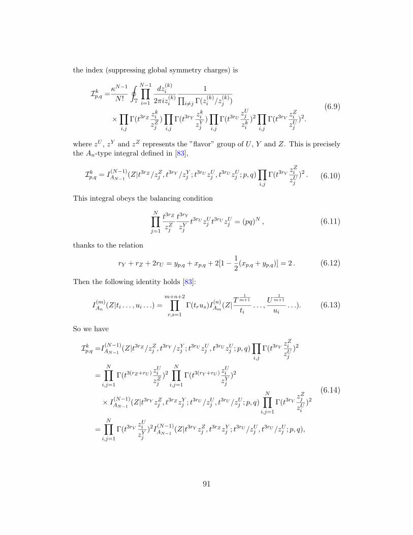
the index (suppressing global symmetry charges) is
Ikp,q =
κN−1
N !
∮T
N−1∏i=1
dz(k)i
2πiz(k)i
1∏i=j Γ(z
(k)i /z
(k)j )
×∏i,j
Γ(t3rZzkizZj
)∏i,j
Γ(t3rYzkizYj
)∏i,j
Γ(t3rUzUj
zki)2∏i,j
Γ(t3rVzZizUj
)2.
(6.9)
where zU , zY and zZ represents the ”flavor” group of U , Y and Z. This is preciselythe An-type integral defined in [83],
Ikp,q = I
(N−1)AN−1
(Z|t3rZ/zZj , t3rY /zYj ; t3rU zUj , t3rU zUj ; p, q)∏i,j
Γ(t3rVzZizUj
)2 . (6.10)
This integral obeys the balancing condition
N∏j=1
t3rZ
zZj
t3rY
zYjt3rU zUj t
3rU zUj = (pq)N , (6.11)
thanks to the relation
rY + rZ + 2rU = yp,q + xp,q + 2[1− 1
2(xp,q + yp,q)] = 2 . (6.12)
Then the following identity holds [83]:
I(m)An
(Z|ti . . . , ui . . .) =m+n+2∏r,s=1
Γ(trus)I(n)Am
(Z|T1
m+1
ti. . . ,
U1
m+1
ui. . .). (6.13)
So we have
Ikp,q =I
(N−1)AN−1
(Z|t3rZ/zZj , t3rY /zYj ; t3rU zUj , t3rU zUj ; p, q)∏i,j
Γ(t3rVzZizUj
)2
=N∏
i,j=1
Γ(t3(rZ+rU ) zUi
zZj)2
N∏i,j=1
Γ(t3(rY +rU ) zUi
zYj)2
× I(N−1)AN−1
(Z|t3rY zZj , t3rZzYj ; t3rU /zUj , t3rU /zUj ; p, q)N∏
i,j=1
Γ(t3rVzZj
zUi)2
=N∏
i,j=1
Γ(t3rVzUizYj
)2I(N−1)AN−1
(Z|t3rY zZj , t3rZzYj ; t3rU /zUj , t3rU /zUj ; p, q),
(6.14)
91
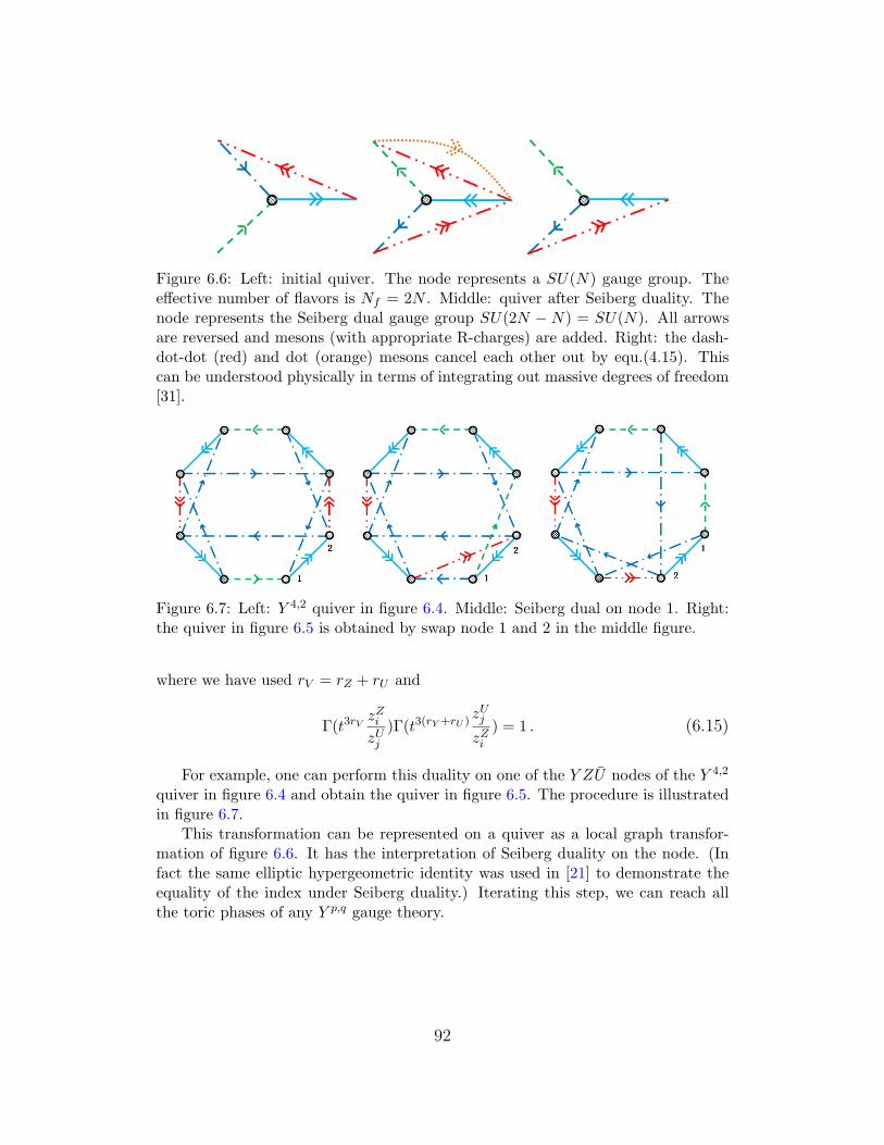
Figure 6.6: Left: initial quiver. The node represents a SU(N) gauge group. Theeffective number of flavors is Nf = 2N . Middle: quiver after Seiberg duality. Thenode represents the Seiberg dual gauge group SU(2N − N) = SU(N). All arrowsare reversed and mesons (with appropriate R-charges) are added. Right: the dash-dot-dot (red) and dot (orange) mesons cancel each other out by equ.(4.15). Thiscan be understood physically in terms of integrating out massive degrees of freedom[31].
Figure 6.7: Left: Y 4,2 quiver in figure 6.4. Middle: Seiberg dual on node 1. Right:the quiver in figure 6.5 is obtained by swap node 1 and 2 in the middle figure.
where we have used rV = rZ + rU and
Γ(t3rVzZizUj
)Γ(t3(rY +rU )zUj
zZi) = 1 . (6.15)
For example, one can perform this duality on one of the Y ZU nodes of the Y 4,2
quiver in figure 6.4 and obtain the quiver in figure 6.5. The procedure is illustratedin figure 6.7.
This transformation can be represented on a quiver as a local graph transfor-mation of figure 6.6. It has the interpretation of Seiberg duality on the node. (Infact the same elliptic hypergeometric identity was used in [21] to demonstrate theequality of the index under Seiberg duality.) Iterating this step, we can reach allthe toric phases of any Y p,q gauge theory.
92
6.2 Large N evaluation of the index
In the large N limit the leading contribution to the index is evaluated using matrixmodels techniques (see e.g. [2, 51]). Let eαaiNa
i=1 denote the Na eigenvalues of ua.Then the matrix model integral (2.23) is,
I(x) =∫ ∏
a,i
[dαai] exp
−∑ai=bj
V ab (αai − αbj)
. (6.16)
Here, the potential V is the following function
V ab (θ) = δab (ln 2) +
∞∑n=1
1
n[δab − iab (x
n)] cosnθ , (6.17)
where, iab (x) is the total single letter index in the representation ra ⊗ rb. Writingthe density of the eigenvalues eαai at the point θ on the circle as ρa(θ), we reduceit to the functional integral problem,
I(x) =∫ ∏
a
[dρa] exp−∫dθ1dθ2
∑a,b
nanbρa(θ1)Vab (θ1 − θ2)ρ
†b(θ2) . (6.18)
For large N , we can evaluate this expression with the saddle point approximation,
I(x) =∏k
1
det(1− i(xk)).
For SU(N) gauge groups instead of U(N), the result is modified as follows,
I(x) =∏k
e−1ktr i(xk)
det(1− i(xk)). (6.19)
Here i(x) is the matrix with entries iab (x). We will see examples of such matricesbelow.
The single-trace partition function can be obtained from the full partition func-tion,
Is.t. =∞∑n=1
µ(n)
nlog I(xn)
= −∞∑k=1
φ(k)
klog[det(1− i(xk))]−
∞∑n=1
µ(n)
n
∞∑k=1
tr i(xnk)
k(6.20)
= −∞∑k=1
φ(k)
klog[det(1− i(xk))]− tr i(x) .
93
The second term in the summation would be absent for the U(N) gauge theories.Here µ(n) is the Mobius function (µ(1) ≡ 1, µ(n) ≡ 0 if n has repeated prime factorsand µ(n) ≡ (−1)k if n is the product of k distinct primes) and φ(n) is the Euler Phifunction, defined as the number of positive integers less than n that are coprime ton. We have used the properties∑
d|n
dµ(n
d) = φ(n),
∑d|n
µ(d) = δn,1. (6.21)
After deriving the general expression for the superconformal index of a quivergauge theory let us study some concrete examples. Recall the single-letter indices
iV (t, y) =2t6 − t3(y + 1
y )
(1− t3y)(1− t3y−1),
iχ(r)(t, y) =t3r
(1− t3y)(1− t3y−1)iχ(r)(t, y) = − t3(2−r)
(1− t3y)(1− t3y−1),
(6.22)
where for future convenience we have split the index of the matter multiplet into achiral and an antichiral contribution. Let us write down explicit expressions for theindex in some examples
• Y 1,0 (T 1,1)
For the conifold gauge theory, U(1)s is enhanced to SU(2)s so the global symmetryis SU(2)s × SU(2)l. Assigning the chemical potentials a and b, for the two SU(2)s,the single letter index matrix i1,0(t, y) is
i1,0 =
iV (a+ 1a)(iχ( 12 )
+ iχ( 12))
(b+ 1b )(iχ( 12 )
+ iχ( 12)) iV
, (6.23)
and the single-trace index evaluates to
Is.t. = −∞∑k=1
φ(k)
klog[(1− iV (x
k))2 − (a+1
a)(b+
1
b)(iχ( 1
2 )(xk) + iχ( 1
2 )(xk))2]− 2iV (x)
=t3ab
1− t3ab+
t3 ab
1− t3 ab
+t3 b
a
1− t3 ba
+t3 1
ab
1− t3 1ab
. (6.24)
This is the index for the theory where both the overall and the relative U(1) degreesof freedom have been removed. The overall U(1) is completely decoupled, while therelative U(1) has positive beta function and decouples in the IR. The removal of therelative U(1) introduces certain double-trace terms in the superpotential which areimportant to achieve exact conformality [124]. We have used the following property
94
of Euler Phi function.∞∑k=1
φ(k)
klog(1− xk) =
−x1− x
. (6.25)
We will match the expression (6.24) to the gravity computation.
• Y 1,1 (C2/Z2 × C)The index for this theory was already obtained in [42, 97]. The single letter indexmatrix i1,1(t, y) is given by
i1,1 =
iV + a−1iχ( 23) + aiχ( 2
3) (b+ 1
b )(aiχ( 23 )+ iχ( 2
3))
(b+ 1b )(iχ( 23 )
+ a−1iχ( 23)) iV + a−1iχ( 2
3) + a iχ( 2
3)
, (6.26)
and the index evaluates to
Is.t. =−∞∑
k=1
φ(k)
klog[(1− iV (xk)− a−1iχ( 2
3)(x
k)− a iχ( 23)(x
k))2 − (b+1
b)2
1
a(a iχ( 2
3)(x
k) + iχ( 23)(x
k))2]
− 2(iV (x) + a−1 iχ( 23)(x) + a iχ( 2
3)(x))
=2t2a
1− t2a+
t4b2a−1
1− t4b2a−1+
t4b−2a−1
1− t4b−2a−1− 2
a t2 − a−1 t4
(1− t3y)(1− t3y−1).
(6.27)
Again, we have subtracted both the overall and relative U(1) degrees of freedom(in this case it is appropriate to subtract N = 2 vector multiplets).
• General Y p,q
A simple generalization gives the index for Y p,0 (T 1,1/Zp) and for Y p,p (C3/Z2p),
Y p,p : det (1− i(t)) =(1− t4p)2(1− t2p)2
(1− t3y)2p(1− t3y−1)2p, (6.28)
Y p,0 : det (1− i(t)) =(1− t3p)4
(1− t3y)2p(1− t3y−1)2p.
In fact the determinant of the adjacency matrix appears to factorize for generalY p,q, to give2
det (1− i(t)) =
[1− t3p(1+
12(xp,q−yp,q))
]2 [1− t3p+
3q2 (1−
12(xp,q+yp,q))
]2(1− t3y)2p(1− t3y−1)2p
. (6.29)
2We have checked this result in several cases but have not attempted an analytic proof.
95
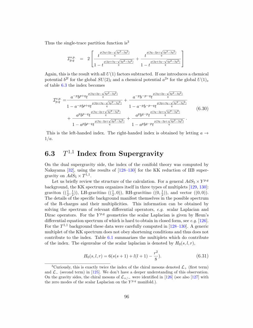
Thus the single-trace partition function is3
Is.p.p,q = 2
tp(3q+2p−
√4p2−3q2)
q
1− tp(2p+3q−
√4p2−3q2)
q
+tp(3q−2p+
√4p2−3q2)
q
1− tp(2p+3q−
√4p2−3q2)
q
Again, this is the result with all U(1) factors subtracted. If one introduces a chemicalpotential b2l for the global SU(2)l and a chemical potential a2s for the global U(1)sof table 6.3 the index becomes
Is.p.p,q =
a−pbp+qtp(3q+2p−
√4p2−3q2)
q
1− a−pbp+qtp(2p+3q−
√4p2−3q2)
q
+a−pb−p−qt
p(3q+2p−√
4p2−3q2)q
1− a−pb−p−qtp(2p+3q−
√4p2−3q2)
q
+apbp−qt
p(3q−2p+√
4p2−3q2)q
1− apbp−qtp(3q−2p+
√4p2−3q2)
q
+apbq−pt
p(3q−2p+√
4p2−3q2)q
1− apbq−ptp(3q−2p+
√4p2−3q2)
q
.
(6.30)
This is the left-handed index. The right-handed index is obtained by letting a →1/a.
6.3 T 1,1 Index from Supergravity
On the dual supergravity side, the index of the conifold theory was computed byNakayama [32], using the results of [128–130] for the KK reduction of IIB super-gravity on AdS5 × T 1,1.
Let us briefly review the structure of the calculation. For a general AdS5 ×Y p,q
background, the KK spectrum organizes itself in three types of multiplets [129, 130]:graviton ((12 ,
12)), LH-gravitino ((12 , 0)), RH-gravitino ((0, 12)), and vector ((0, 0)).
The details of the specific background manifest themselves in the possible spectrumof the R-charges and their multiplicities. This information can be obtained bysolving the spectrum of relevant differential operators, e.g. scalar Laplacian andDirac operators. For the Y p,q geometries the scalar Laplacian is given by Heun’sdifferential equation spectrum of which is hard to obtain in closed form, see e.g. [126].For the T 1,1 background these data were carefully computed in [128–130]. A genericmultiplet of the KK spectrum does not obey shortening conditions and thus does notcontribute to the index. Table 6.1 summarizes the multiplets which do contributeof the index. The eigenvalue of the scalar laplacian is denoted by H0(s, l, r),
H0(s, l, r) = 6(s(s+ 1) + l(l + 1)− r2
8). (6.31)
3Curiously, this is exactly twice the index of the chiral mesons denoted L+ (first term)and L− (second term) in [125]. We don’t have a deeper understanding of this observation.On the gravity sides, the chiral mesons of L+/− were identified in [126] (see also [127] withthe zero modes of the scalar Laplacian on the Y p,q manifold.).
96
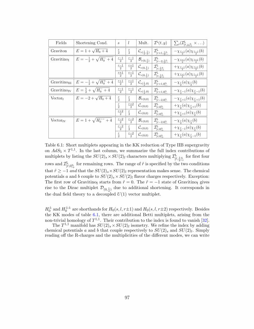
Fields Shortening Cond. s l Mult. IL(t, y)∑
r(IL[r,j2]L+
× . . .)
Graviton E = 1 +√H0 + 4 r
2r2
Cr( 12, 12) IL
[r+1, 12]L−
−χ r−12(a)χ r−1
2(b)
GravitinoI E = −12+√H−
0 + 4 r−12
r−12
Br(0, 12) IL
[r−2, 12]L−
−χ r+12(a)χ r+1
2(b)
r−12
r+12
Cr(0, 12) IL
[r, 12]L+
+χ r−12(a)χ r+1
2(b)
r+12
r−12
Cr(0, 12) IL
[r, 12]L+
+χ r+12(a)χ r−1
2(b)
GravitinoIII E = −12+√H+
0 + 4 r+12
r+12
Cr( 12,0) IL
[r+1,0]L−−χ r
2(a)χ r
2(b)
GravitinoIV E = 52+√H−
0 + 4 r−12
r−12
Cr( 12,0) IL
[r+1,0]L−−χ r
2−1(a)χ r
2−1(b)
VectorI E = −2 +√H0 + 4 r
2r2
Br(0,0) IL[r−2,0]L−
−χ r2+1(a)χ r
2+1(b)
r2
r+22
Cr(0,0) IL[r,0]L+
+χ r2(a)χ r
2+1(b)
r+22
r2
Cr(0,0) IL[r,0]L+
+χ r2+1(a)χ r
2(b)
VectorIV E = 1 +√H−−
0 + 4 r−22
r−22
Br(0,0) IL[r−2,0]L−
−χ r2(a)χ r
2(b)
r−22
r2
Cr(0,0) IL[r,0]L+
+χ r2−1(a)χ r
2(b)
r2
r−22
Cr(0,0) IL[r,0]L+
+χ r2(a)χ r
2−1(b)
Table 6.1: Short multiplets appearing in the KK reduction of Type IIB supergravityon AdS5 × T 1,1. In the last column, we summarize the full index contributions ofmultiplets by listing the SU(2)s×SU(2)l characters multiplying IL
[r, 12]L+
for first four
rows and IL[r,0]L+
for remaining rows. The range of r is specified by the two conditions
that r ≥ −1 and that the SU(2)s×SU(2)l representation makes sense. The chemicalpotentials a and b couple to SU(2)s×SU(2)l flavor charges respectively. Exception:The first row of GravitinoI starts from r = 0. The r = −1 state of GravitinoI givesrise to the Dirac multiplet D(0, 1
2) due to additional shortening. It corresponds in
the dual field theory to a decoupled U(1) vector multiplet.
H±0 andH±±
0 are shorthands forH0(s, l, r±1) andH0(s, l, r±2) respectively. Besidesthe KK modes of table 6.1, there are additional Betti multiplets, arising from thenon-trivial homology of T 1,1. Their contribution to the index is found to vanish [32].
The T 1,1 manifold has SU(2)s×SU(2)l isometry. We refine the index by addingchemical potentials a and b that couple respectively to SU(2)s and SU(2)l. Simplyreading off the R-charges and the multiplicities of the different modes, we can write
97
down the index as [32]4
IL =−∑r≥0
IL[r, 12 ]
L+[(ab)r+1 + (
a
b)r+1 + (
b
a)r+1 + (
1
ab)r+1]
−∑r≥−1
IL[r,0]L+
[(ab)r + (a
b)r + (
b
a)r + (
1
ab)r + (ab)r+2 + (
a
b)r+2 + (
b
a)r+2 + (
1
ab)r+2]
+ IL[−1,0]L+
χ− 32(a)χ− 3
2(b)− IL
[0,0]L+[−χ−1(a)χ−1(b) + χ−1(a)χ0(b) + χ0(a)χ−1(b)]
(6.32)
The definition of the index building blocks IL[r,j2]L±
is given in appendix D, while
the symbol χj(x) stands for the standard character of the spin-j representation ofSU(2),
χj(x) ≡x2j+1 − x−(2j+1)
x− x−1. (6.33)
After simplification,
IL =t3ab
1− t3ab+
t3 ab1− t3 ab
+t3 b
a
1− t3 ba
+t3 1
ab
1− t3 1ab
, (6.34)
which precisely agrees with the large N index (6.24) computed from gauge theoryusing Romelsberger’s prescription.
4On the field theory side, we subtracted both U(1) factors. Correspondingly, on thegravity side we should subtract all singleton degrees of freedom, and thus omit the r = −1mode of the GravitinoI tower, which corresponds to a D(0,1/2) multiplet.
98
Chapter 7
Discussion
In this thesis we have discussed an important observable related to the spectrumof superconformal field theories - the superconformal index. Computed exactly bylocalization technique, the superconformal index captures of the information aboutthe protected spectrum of the theory.
We have defined and studied several limits of the N = 2 superconformal index.They are characterized by enhanced supersymmetry and depend at most on twosuperconformal fugacities, out of the possible three. We have given a prescriptionto calculate these limits for all A-series superconformal quivers of class S, even whenthey lack a Lagrangian description. Thanks to the topological QFT structure of theindex, it suffices to find a formula for the elementary three-valent building blocks.For the SU(2) quivers, which do have a Lagrangian description, the building block-s can be written in terms of algebraic objects that admit a natural extrapolationto higher rank, leading to a compelling general conjecture that passes many tests.These objects are the Macdonald polynomials, tailor-made for our purposes as theydepend on two fugacities, and for which a beautiful general theory is already avail-able. We expect the generalization of our results to the D-series quivers of class S(and possibly to the E-series as well) to be straightforward.
The TQFT that calculates the index of the Ak−1 quivers is closely related totwo-dimensional Yang-Mills theory with gauge group SU(k). An immediate qual-itative hint, of course, is that the state-space of the index TQFT is the space ofirreducible SU(k) representations. As first discussed in [17], and confirmed herein more generality, there is in fact a precise quantitative correspondence betweenthe limit of the index that we have dubbed the “Schur index”, which depends ona single fugacity q, and correlators of q-deformed 2d Yang-Mills theory [101] in thezero-area limit. In turn, the zero-area limit of q-deformed 2d Yang-Mills on the Rie-mann surface C can be viewed as an analytic continuation of Chern-Simons theoryon C × S1 [101].
Recently, a “refinement” of Chern-Simons theory on three-manifolds admitting acircle action was defined in [107], via the relation with topological string theory andits embedding into M-theory. Taking the three-manifold to be of the form C × S1,
99
and reducing on the S1, one obtains an indirect definition of “refined q-deformedYang-Mills theory” on C, which depends on two parameters q and t. (The defini-tion is indirect because unlike the purely q-deformed case no Lagrangian descriptionis available for the refined theory.) The refinement essentially amounts to trad-ing Schur polynomials with Macdonald polynomials, and we have found a preciserelation between our (q, t) “Macdonald index” and correlators of this (q, t)-Yang-Mills theory. It is natural to ask whether this is pointing to a direct connectionbetween topological string theory and the superconformal index. At first sight thegeometries involved appear to be quite different, since to obtain the superconformalindex we must consider the (2, 0) theory on S3 × S1 × C, with appropriate twistsinduced by the fugacities, while in the setup of [6, 107] the relevant geometry is(C × S1 ×M3)q,t, where one may take M3 = S1 × C (we refer to the cited papersfor a proper explanation). Moreover while the index admits a further refinement fora total of three fugacities, it seems difficult to introduce a third parameter in theframework of [6, 107] while preserving supersymmetry. Nevertheless, at least for thespecial case of the Macdonald index, there should be a deeper way to understandthe striking similarity of the two results.
An obvious direction for future work is the generalization of our results to thefull three-parameter index. The Haar measure together with the index of the N = 2vector multiplet combine to [16, 21]
1
k!
k∏i,j=1,i =j
1
Γ (xi/xj ; q, p) Γ (t xi/xj ; q, p), (7.1)
where Γ(z; p, q) is the elliptic Gamma function
Γ(z; p, q) =
∞∏i,j=0
1− pi+1qj+1/z
1− piqjz. (7.2)
A natural speculation is that the functions fλp,q,t(a) that diagonalize the structureconstants of the full index should be proportional to elliptic extensions of the Mac-donald polynomials, to which they should reduce in the limit p → 0 (or q → 0).Various proposals for elliptic Macdonald functions have appeared in the mathe-matical literature, see e.g. [83, 131, 132]. We can in fact formulate a more preciseconjecture, motivated by the relation between two-dimensional gauge theories andintegrable quantum mechanical models of Calogero-Moser (CM) type, see e.g. [133–138]. The reduction of ordinary 2d Yang-Mills theory to one dimension yields therational (non-relativistic) CM model [133]. One can consider the trigonometricand elliptic generalizations of the non-relativistic model, as well as their relativis-tic cousins (the relativistic versions are also known as Ruijsenaars-Schneider (RS)models). The relativistic trigonometric model (trigonometric RS) depends on twoparameters (q, t), has Macdonald polynomials as its eigenfunctions, and is closely
100
related to the two-dimensional G/G WZW model1 or equivalently to Chern-Simonstheory on C × S1. At the summit of this hierarchy is the elliptic relativistic model(elliptic RS), which depends on three parameters, analogous to (p, q, t) of the fullindex. Our conjecture is then that the symmetric functions relevant for the com-putation of the full index are the eigenfunctions of the elliptic RS model. Not toomuch is known about them, see [140] for a review.2
Perhaps the most interesting open problem is to give a “microscopic” derivationof the two-dimensional TQFT of the index from the six-dimensional (2, 0) theory.A promising shortcut, which exploits the mentioned connection between 2d gaugetheories and 1d Calogero-Moser models, is along the following lines. Consider the(2, 0) theory on S3 × S1
(1) × Cg,s. The Riemann surface Cg,s can be viewed as a
circle, S1(2), times a graph Ig,s By first reducing the (2, 0) theory on S1
(2) (note that
there is no twist around this circle) one obtains 5d super Yang-Mills on S3 × S1(1) ×
Ig,s. We propose that the further reduction of 5d SYM on S1(1) × S3 (with the
fugacity twists) yields the elliptic RS model on the graph Ig,s, with appropriateboundary conditions at the s external punctures and at the internal junctures. In asuitable limit, which corresponds to taking S1
(1) to be small, the 4d index becomes
the 3d partition function [103–105], and our proposal reduces to the one of [114](see also [113]). These authors show how to interpret such 3d partition functions asoverlaps of quantum mechanical wave functions. We are suggesting that a similaridea may apply to the 4d index, and that the relevant quantum mechanical modelis the elliptic RS model. More work is going to be done along these lines.
1See [137] for a review and [139] for recent relevant work.2Quantum mechanical integrable models have been recently related to the problem of
counting vacua of N = 2 supersymmetric theories in the Ω-background [141, 142]. Seealso [143, 144] for connections of elliptic Gamma functions to integrable systems.
101
Appendix A
Duality
A.1 The Representation Basis
The labels of the topological algebra as we have defined in (3.6) are (compact) con-tinuous parameters αi ∈ [0, 2π). We can “Fourier” transform to the discrete basis ofirreducible SU(2) representations. We denote by RK the irreducible representationof SU(2) of dimension K+1. The integrals over characters translate into sums overrepresentations. The structure constants in the discrete basis are given by
Cαβγ =∞∑
K,L,M=0
sin(K + 1)α
sinα
sin(L+ 1)β
sinβ
sin(M + 1)γ
sin γCKLM (A.1)
=
∞∑K,L,M=0
χK(α)χL(β)χM (γ) CKLM ,
where χK(α) is the character of RK ,
χK(α) =sin(K + 1)α
sinα. (A.2)
Similarly the metric in the discrete basis is given by
ηαβ =
∞∑K,L=0
χK(α)χL(β) ηKL . (A.3)
102
Further, we define the scalar product of characters1
⟨χK χM ⟩ = 1
2πi
∮dz
z(1− z2)χK(z)χM (z)
= − 1
4πi
∮dz
z(z − 1
z)2 χK(z)χM (z) =
∫ 2π
0dθ∆(θ)χK(θ)χM (θ) = δK,M
(A.4)
In the second equality we have introduced the measure (3.5) and used the fact thatχ(z) = χ(z−1). Thus we have
∞∑K=0
χK(α)χK(β) = δ(α, β),
∫ 2π
0dθ∆(θ) δ(θ, α) f(θ) = f(α), (A.5)
for any f obeying f(θ) = f(−θ). Using (3.6) we can write
ηKL = ηI⟨χIχKχL⟩, ηI =
∫dα∆(α) ηα χI(α). (A.6)
Finally with the help of these definitions, we can rewrite (3.8) as
I =∏
i,j,k∈V
CLiLjLk
∏m,n∈G
ηLmLn , (A.7)
where index contractions now indicate sums over the non-negative integers.
A.2 TQFT Algebra for v = t
For v = t we can rewrite the algebra of the topological quantum field theory (3.6) ina more elegant way, removing the delta-functions by making use of identities obeyedby elliptic Beta integrals. This does not appear to be a preferred limit physically,except for the fact that the contribution to the index of the chiral superfield in theN = 2 vector multiplet vanishes, see (2.13). Our manipulations will be slightlyformal since the limit v = t of the formulae we will use is somewhat singular. Westart by quoting the important identity
E(m=0)(t1, . . . , t6) =κ
∮dz
z
∏6k=1 Γ
(tk z
±1; p, q)
Γ (z±2; p, q)=
∏1≤j<k≤6
Γ (tj tk; p, q) ,
6∏k=1
tk = pq
(A.8)
1We have a slightly different convention for the characters and thus the expression ofthe scalar product differs from the one in [145].
103
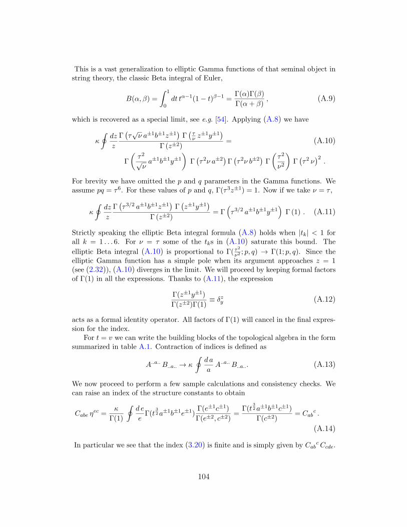
This is a vast generalization to elliptic Gamma functions of that seminal object instring theory, the classic Beta integral of Euler,
B(α, β) =
∫ 1
0dt tα−1(1− t)β−1 =
Γ(α)Γ(β)
Γ(α+ β), (A.9)
which is recovered as a special limit, see e.g. [54]. Applying (A.8) we have
κ
∮dz
z
Γ(τ√ν a±1b±1z±1
)Γ(τν z
±1y±1)
Γ (z±2)= (A.10)
Γ
(τ2√νa±1b±1y±1
)Γ(τ2ν a±2
)Γ(τ2ν b±2
)Γ
(τ2
ν2
)Γ(τ2 ν
)2.
For brevity we have omitted the p and q parameters in the Gamma functions. Weassume pq = τ6. For these values of p and q, Γ(τ3z±1) = 1. Now if we take ν = τ ,
κ
∮dz
z
Γ(τ3/2 a±1b±1z±1
)Γ(z±1y±1
)Γ (z±2)
= Γ(τ3/2 a±1b±1y±1
)Γ (1) . (A.11)
Strictly speaking the elliptic Beta integral formula (A.8) holds when |tk| < 1 forall k = 1 . . . 6. For ν = τ some of the tks in (A.10) saturate this bound. The
elliptic Beta integral (A.10) is proportional to Γ( τ2
ν2; p, q) → Γ(1; p, q). Since the
elliptic Gamma function has a simple pole when its argument approaches z = 1(see (2.32)), (A.10) diverges in the limit. We will proceed by keeping formal factorsof Γ(1) in all the expressions. Thanks to (A.11), the expression
Γ(z±1y±1)
Γ(z±2)Γ(1)≡ δzy (A.12)
acts as a formal identity operator. All factors of Γ(1) will cancel in the final expres-sion for the index.
For t = v we can write the building blocks of the topological algebra in the formsummarized in table A.1. Contraction of indices is defined as
A..a..B..a.. → κ
∮d a
aA..a..B..a... (A.13)
We now proceed to perform a few sample calculations and consistency checks. Wecan raise an index of the structure constants to obtain
Cabe ηec =
κ
Γ(1)
∮d e
eΓ(t
32a±1b±1e±1)
Γ(e±1c±1)
Γ(e±2, c±2)=
Γ(t32a±1b±1c±1)
Γ(c±2)= Cab
c .
(A.14)
In particular we see that the index (3.20) is finite and is simply given by CabcCcde.
104
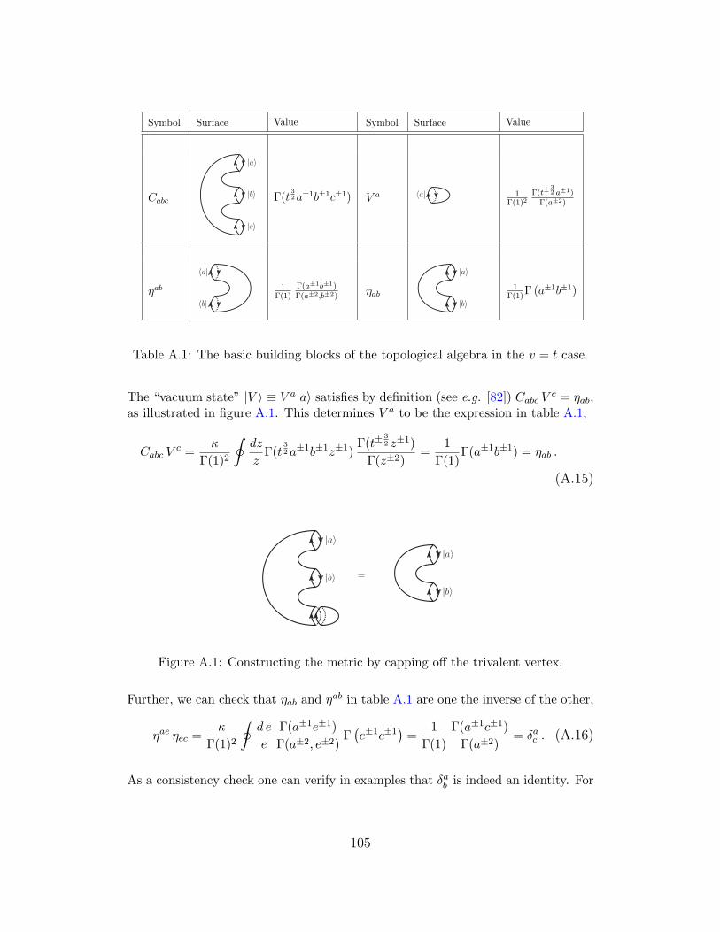
Symbol Surface Value Symbol Surface Value
Cabc
|a〉
|b〉
|c〉
Γ(t32a±1b±1c±1) V a 〈a| 1
Γ(1)2Γ(t±
32 a±1)
Γ(a±2)
ηab
〈a|
〈b|
1Γ(1)
Γ(a±1b±1)Γ(a±2,b±2) ηab
|a〉
|b〉
1Γ(1)
Γ (a±1b±1)
Table A.1: The basic building blocks of the topological algebra in the v = t case.
The “vacuum state” |V ⟩ ≡ V a|a⟩ satisfies by definition (see e.g. [82]) Cabc Vc = ηab,
as illustrated in figure A.1. This determines V a to be the expression in table A.1,
Cabc Vc =
κ
Γ(1)2
∮dz
zΓ(t
32a±1b±1z±1)
Γ(t±32 z±1)
Γ(z±2)=
1
Γ(1)Γ(a±1b±1) = ηab .
(A.15)
|a〉
|b〉
|a〉
|b〉
=
Figure A.1: Constructing the metric by capping off the trivalent vertex.
Further, we can check that ηab and ηab in table A.1 are one the inverse of the other,
ηae ηec =κ
Γ(1)2
∮d e
e
Γ(a±1e±1)
Γ(a±2, e±2)Γ(e±1c±1
)=
1
Γ(1)
Γ(a±1c±1)
Γ(a±2)= δac . (A.16)
As a consistency check one can verify in examples that δab is indeed an identity. For
105
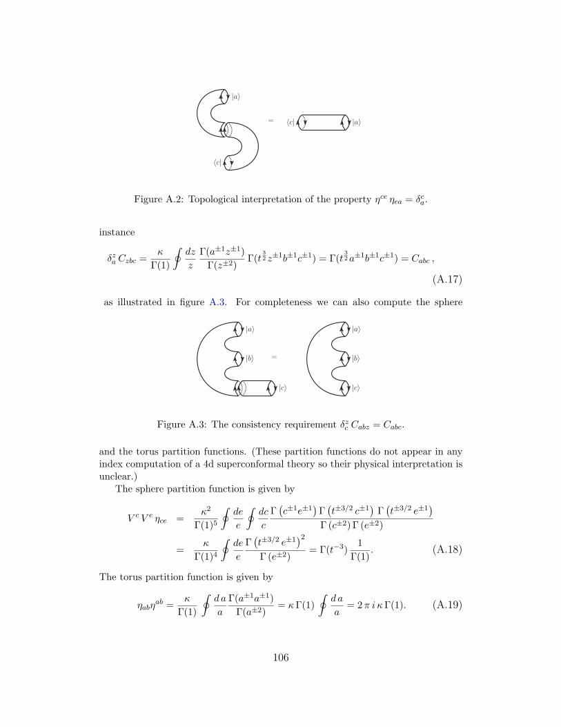
|a〉
〈c|
〈c| |a〉=
Figure A.2: Topological interpretation of the property ηce ηea = δca.
instance
δza Czbc =κ
Γ(1)
∮dz
z
Γ(a±1z±1)
Γ(z±2)Γ(t
32 z±1b±1c±1) = Γ(t
32a±1b±1c±1) = Cabc ,
(A.17)
as illustrated in figure A.3. For completeness we can also compute the sphere
|a〉
|b〉 =
|c〉
|a〉
|b〉
|c〉
Figure A.3: The consistency requirement δzc Cabz = Cabc.
and the torus partition functions. (These partition functions do not appear in anyindex computation of a 4d superconformal theory so their physical interpretation isunclear.)
The sphere partition function is given by
V c V e ηce =κ2
Γ(1)5
∮de
e
∮dc
c
Γ(c±1e±1
)Γ(t±3/2 c±1
)Γ(t±3/2 e±1
)Γ (c±2) Γ (e±2)
=κ
Γ(1)4
∮de
e
Γ(t±3/2 e±1
)2Γ (e±2)
= Γ(t−3)1
Γ(1). (A.18)
The torus partition function is given by
ηabηab =
κ
Γ(1)
∮d a
a
Γ(a±1a±1)
Γ(a±2)= κΓ(1)
∮d a
a= 2π i κΓ(1). (A.19)
106
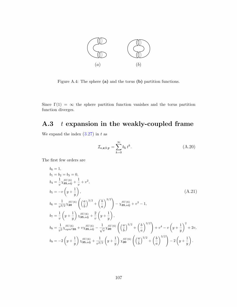
(a) (b)
Figure A.4: The sphere (a) and the torus (b) partition functions.
Since Γ(1) = ∞ the sphere partition function vanishes and the torus partitionfunction diverges.
A.3 t expansion in the weakly-coupled frame
We expand the index (3.27) in t as
Ia,z;b,y =
∞∑k=0
bk tk. (A.20)
The first few orders are
b0 = 1,
b1 = b2 = b3 = 0,
b4 =1
vχSU(6)35,adj +
1
v+ v2,
b5 = −v(y +
1
y
), (A.21)
b6 =1
v3/2χSU(6)20
((ab
)3/2+
(b
a
)3/2)
− χSU(6)35,adj + v3 − 1,
b7 =1
v
(y +
1
y
)χSU(6)35,adj +
2
v
(y +
1
y
),
b8 =1
v2χSU(6)sym235 + vχ
SU(6)35,adj −
1√vχSU(6)20
((ab
)3/2+
(b
a
)3/2)
+ v4 − v
(y +
1
y
)2
+ 2v,
b9 = −2
(y +
1
y
)χSU(6)35,adj +
1
v3/2
(y +
1
y
)χSU(6)20
((ab
)3/2+
(b
a
)3/2)
− 2
(y +
1
y
).
107
In the above equation we decomposed SU(6) ⊃ SU(3)z ⊗ SU(3)y−1 ⊗ U(1). Thebranching of 35 and 20 of SU(6) is given by (see [146]),
35 = (1,1)0 + (8,1)0 + (1,8)0 + (3,3)2 + (3, 3)−2 , (A.22)
20 = (1,1)3 + (1,1)−3 + (3,3)−1 + (3, 3)1 .
For example, the character of the adjoint is
χSU(6)35,adj =
[(a b)1/2 (z1 + z2 + z3) + (a b)−1/2 (
1
y1+
1
y2+
1
y3)
](A.23)
×[(a b)−1/2
(1
z1+
1
z2+
1
z3
)+ (a b)1/2 (y1 + y2 + y3)
]− 1 .
We conclude that the U(1) charge in SU(6) can be identified as (a b)−1/2.
A.4 Inversion theorem
In this appendix we quote the inversion theorem [78], which we use in section 3.2.2to obtain the index of the E6 theory. Define
δ(z, w;T ) ≡ Γ(T z±1w±1; p, q)
Γ(T 2, z±2; p, q). (A.24)
If T , p and q are such that
|max(p, q)| < |T | < 1 , (A.25)
then the following theorem holds true. For fixed w on the unit circle we define acontour Cw (see figure A.5) in the annulus A = |T |−ϵ < |z| < |T |−1+ϵ with smallbut finite ϵ ∈ R+, such that the points T−1w±1 are in its interior and Cw = C−1
w(i.e. an inverse of the point in the interior of Cw is in the exterior of Cw). Letf(z) = f(z−1) be a holomorphic function in A. Then for |T | < |x| < |T |−1,
f(w) = κ
∮Cw
dz
2πi zδ(z, w; , T−1) f(z) −→ f(x) = κ
∮T
dw
2πiwδ(w, x; , T ) f(w) .
(A.26)
Our expression for the index in the strongly-coupled frame (3.37) is of the formof the right hand side of (A.26). Thus, to use the inversion theorem to obtain theindex of E6 theory we assume that this index can be written as
Γ(t2v w±2) C(E6) ((w, r),y, z) = κ
∮Cw
ds
2πi s
Γ(√v
t2w±1 s±1)
Γ( vt4, s±2)
F (s, r;y, z) ,
(A.27)
108
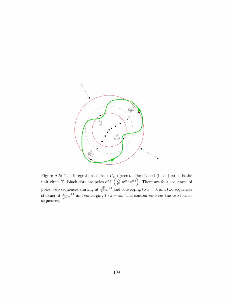
t2w
√
v
√
v
t2w
t2
w√
v
w√
v
t2
Figure A.5: The integration contour Cw (green). The dashed (black) circle is the
unit circle T. Black dots are poles of Γ(√
vt2w±1 z±1
). There are four sequences of
poles: two sequences starting at√v
t2w±1 and converging to z = 0, and two sequences
starting at t2√vw±1 and converging to z = ∞. The contour encloses the two former
sequences.
109
for some function F . The theorem (A.26) then implies that F (s, r;y, z) = I (s, r;y, z)with I (s, r;y, z) given in (3.37).
A.5 The Coulomb and Higgs branch operators
of E6 SCFT
We collect here a few facts about the Coulomb and the Higgs branches of E6 SCFT,following the analysis of [80]. Argyres-Seiberg duality can be used to determine thequantum numbers of protected operators of E6 theory if their dual operators in thedual SU(3) theory are known. The Coulomb branch operator u of the E6 theory(the operator whose vev parametrized the Coulomb branch) is identified as Trϕ3 inthe SU(3) theory. Since ϕ has quantum numbers (E, j1, j2, R, r) = (1, 0, 0, 0,−1), ushould have quantum numbers (3, 0, 0, 0,−3) and contribute to the superconformalindex as t6v3.
The operator X whose vev parametrized the Higgs branch transforms in theadjoint representation of E6. Under the SU(2)⊗SU(6) subgroup of E6 it decomposesas
Xij , Y [ijk]
α , Zαβ , (A.28)
where i, j, k = 1, . . . , 6 are the SU(6) indices, and α, β = 1, 2 are the SU(2) indices.At the same time, the SU(2) gauge theory provides the quarks qα, qα and the F -termconstraint
Zαβ + q(αqβ) = 0 . (A.29)
Thus the gauge-invariant operators are
(qq), Xij , (Y ijkq), (Yijkq) . (A.30)
On the SU(3) side, the Higgs branch is parameterized by gauge invariant oper-ators
M ij = Qi
aQaj , Bijk = ϵabcQi
aQjbQ
kc , Bijk = ϵabcQ
ai Q
bjQ
ck , (A.31)
where Qia and Qa
i are the squark fields, i = 1, . . . , 6 are flavor indices, and a = 1, 2, 3the color indices.
The duality of the two sides suggests the following identification
TrM ↔ (qq), M ij ↔ Xi
j , (A.32)
Bijk ↔ (Y ijkq), Bijk ↔ (Yijkq) (A.33)
where M ij is the traceless part of M i
j . Since the quantum numbers of Q are(1, 0, 0, 1/2, 0), the quantum numbers of X should be (2, 0, 0, 1, 0), and contribute tothe index as t4/v.
110
A.6 Identities from S-duality
In this appendix we summarize identities of integrals of elliptic Gamma functionsimplied by S-duality of the SU(3) quiver theories.
Generalization of [76]
We define
I(n)(a , zSU(n); b ,ySU(n)
)≡ 2n−1
n!κn−1Γ(t2v)n−1×
∮Tn−1
n−1∏i=1
dxi2πi xi
∏ni=1
∏nj=1 Γ
(t2√v
(azixj
)±1)Γ(
t2√v(b yi xj)
±1)∏
i =j Γ(t2v xi
xj
)∏
i =j Γ(
xi
xj
)∣∣∣∣∣∣∣∣∏n
j=1 xj=1
.
(A.34)
The claim is that
I(n)(a , zSU(n); b ,ySU(n)
)= I(n)
(b , zSU(n); a ,ySU(n)
). (A.35)
For SU(2) this identity was proven in [76], and for SU(3) we have performed per-turbative checks. The usual S-duality of Nf = 2n SU(n) theories implies that thisidentity should be true for any n. Note that for t = v this is a special case ofidentities discussed in [83].
E6 Integral
We define
C(E6) ((w, r),y, z) ≡ 2κ3Γ(t2v)2
3Γ(t2v w±2)
∮Cw
ds
2πi s
Γ(√v
t2 w±1 s±1)
Γ( vt4 , s
±2)×
×∮T2
2∏i=1
dxi2πi xi
3∏i=1
3∏j=1
Γ
t2√v
(s
13 zixj r
)±1Γ
t2√v
(s−
13 yi xjr
)±1∏
i =j
Γ
(t2v
xixj
)∏i =j
Γ
(xixj
) .
(A.36)This integral has manifest symmetry under SU(2)w ⊗SU(6), where the SU(6) hasbeen decomposed as SU(3)z ⊗SU(3)y−1 ⊗U(1)r. The identification with the indexof the E6 SCFT implies that there must be a symmetry enhancement SU(2)w ⊗SU(6) → E6. Two properties that are sufficient to guarantee E6 covariance are:
111
first,
C(E6) ((w, r),y, z) = C(E6)
((w1/2
r3/2,
1
w1/2 r1/2
),y, z
), (A.37)
which is the statement that (w, r) combine into a character of SU(3) (which we shalldenote by w); second,
C(E6)(w,y, z) = C(E6)(y,w, z) . (A.38)
We presented perturbative evidence for the full E6 symmetry in the text.
S-dualities of SU(3) quivers
Define
I3333 (y, z,u, s) ≡∮T2
2∏i=1
dxi2πixi
∏i =j
Γ(t2vxi/xj
)Γ (xi/xj)
C(E6) (y, z,x)C(E6)(u, s,x−1
),
I3331 (y, z,u, a) ≡∮T2
2∏i=1
dxi2πixi
∏i =j
Γ(t2vxi/xj
)Γ (xi/xj)
C(E6) (y, z,x)
3∏i,j=1
Γ
(t2√v
(a x−1
i uj)±)
.
(A.39)
The S-dualities of the SU(3) quivers imply
I3333 (y, z,u, s) = I3333 (y,u, z, s) , (A.40)
I3331 (y, z,u, a) = I3331 (y,u, z, a) .
112
Appendix B
MacDonald
B.1 Construction of the diagonal expression
for the SU(2) HL index
In this appendix we diagonalize the structure constants of the SU(2) quivers in theρ→ 0, σ → 0 limit. With hindsight, we have dubbed this limit the Hall-Littlewood(HL) index, since the diagonal functions turn out to be closely related to the Hall-Littlewood polynomials. This is precisely what we show in this appendix.
For SU(2), the SCFT associated to three-punctured sphere is the the free hy-permultiplet in the trifundamental representation. In the limit of interest, its indexreads
I(a, b, c) = PE [τχ1(a)χ1(b)χ1(c)]a,b,c,τ =1∏
sa,sb,sc=±1(1− τ asa bsb csc), (B.1)
where the fugacities a, b, and c label the Cartans of the three SU(2) flavor groups.The index of the vector multiplet and the SU(2) Haar measure combine to
∆(a)IV (a, τ) = (1− τ2)∆τ2,τ4(a) , (B.2)
where ∆τ2,τ4(a) is the Macdonald measure (4.96) with q = τ2 and t = τ4,
∆τ2,τ4(a) =1
2(1− a2)(1− 1
a2)(1− τ2a2)(1− τ2
a2) . (B.3)
The corresponding Macdonald polynomials P λ(a, a−1; q, t), normalized to be or-
113
thonormal under (B.2), are1
Pλ(a; τ2, τ4) =τ√
1− τ2(1− 1
a2 τ2)(1− a2τ2)
√χλ(τ)χλ+2(τ)
χλ(a)
χλ(τ)− χλ+2(a)
χλ+2(τ)
.
(B.4)
By choosing P λ(a, a−1; q, t) as a basis, the metric of the TQFT is then trivial,ηλµ = δλµ. On the other hand, the projection of I(a, b, c) into the basis functionsgives the structure constants Cµνλ,
I(a, b, c) =∞∑
µ,ν,λ=0
CµνλPµ(a; τ2, τ4)P ν(b; τ2, τ4)P λ(c; τ2, τ4) . (B.5)
We find that while the structure constants are not diagonal, they take a relativelysimple “upper triangular” form. The only non-vanishing coefficients are
Cλλλ ≡ Ψλ , Cλµµ = Cµλµ = Cµµλ ≡ Ωλ for µ < λ , (−1)λ+µ = 1 , (B.6)
where
Ψλ(τ) =
√1− τ2√χλ+2(τ)
(τ−1 + τ√χλ(τ)
− τλ+3√χλ(τ)
), (B.7)
Ωλ(τ) =√
1− τ2(τ−1 + τ)1√
χλ(τ)χλ+2(τ).
Associativity is easy to check. It is trivial for most choices of external states, theone interesting case being the four-point function µµνν with µ < ν and having thesame parity (both even or both odd). Equality of the two channels reads∑
λ≥ν,(−1)λ+µ=1
CµµλCλνν = [Cµµν ]2 , (B.8)
which amounts to (no sum on ν)∑λ>ν,(−1)λ+µ=1
Ωλ(τ)2 +Ων(τ)Ψν(τ) = Ων(τ)
2 . (B.9)
One can verify that this property is satisfied for the particular values of the coeffi-cients given in (B.7).2
Let us now perform an orthogonal transformation that diagonalizes the structure
1This normalization is only used in this appendix. In the rest of the paper Macdonaldpolynomials are taken to have unit norm with respect to the Macdonald measure.
2One needs the identity∑∞
k=01
sinhα(2k+3) sinhα(2k+1) = e−α
2 sinh2 α coshαand induction on
ν.
114
constants. From (B.6) we see even and odd Macdonald polynomials do not mix witheach other and thus can carry our the diagonalization separately for each parity;the discussion below is restricted to the even parity case for definiteness. The Latinletter indices below, j, . . . , run over the integers and correspond to half the value ofthe Greek indices used above.
We define real symmetric matrices Ni as3
(Ni)jk ≡ Cijk . (B.10)
Associativity implies that they commute, [Ni, Nj ] = 0, so they can be simultaneouslydiagonalized. Recall that the structure of each matrix Nj is
(Nj)ik =
i < j, i = k Ωj
i = k = j Ψj
i > j, k = j Ωi
k > j, i = j Ωk
other 0
(B.11)
The non-zero eigenvalues of this matrix are Ωj with multiplicity j, and Ψj −Ωj withmultiplicity one. The unique eigenvector with eigenvalue Ψj − Ωj is
ej+1 = (0, . . . , 0, Ψj − Ωj , Ωj+1, Ωj+2, . . . ) , (B.12)
where there are j zeros in the beginning of the vector. Note that the ejs are orthog-onal to each other,
ej+1 · ek+1 = (Ψj − Ωj)Ωj +∑i>j
[Ωi]2 = 0 , (B.13)
where we took j > k without loss of generality and used the associativity constraint(B.9). Moreover, the vectors ei turn out to be eigenvectors of all the matrices Nj ,
i < j : Nj · ei+1 = Ωj ei+1 , (B.14)
i = j : Nj · ei+1 = (Ψj − Ωj) ei+1 ,
i > j : Nj · ei+1 = 0 .
This can be shown from the definitions with the help of the associativity constraint(B.9). To complete this set of vectors to a basis we have to add one more vector,orthogonal to all ej ,
e0 = (Ω1, Ω2, . . . ) . (B.15)
3Note that since the metric is trivial, ηij = δij , the upper or lower position of the indicesis immaterial.
115
This is an eigenvector of all the matrices Nj with eigenvalue Ωj . We have thusmanaged to diagonalize the matrices Ni. In the diagonal basis ej the matricesare given by (we use hatted indices to represent components in the new basis)
(Nj )ik =
j > i , Ωj δiji = j , (Ψj − Ωj) δijj < i, 0
(B.16)
Finally we perform the orthogonal transformation to the new basis also for thematrix label j of Nj , and find constants in the new basis read
Cjik =1
nj
∑l
(ej)l · (Nl)ik , (B.17)
where nj is the normalization of ej ,
nj =√
ej · ej = τ2j√
1− τ2 for j > 0 , (B.18)
n0 =√e0 · e0 =
√(1− τ2)(1 + τ2) .
A little calculation gives
Ciii = ni , (B.19)
and zero for the other choices of the indices. So far we have restricted attention toeven parity (in terms of the original Greek labels). The case of odd parity worksalong completely parallel lines.
We can now explicitly compute the functions that diagonalize the structureconstants, by contacting the normalized vectors eµ/nµ with the Macdonald polyno-mials (B.4). A useful identity is (λ > 0)
∞∑µ=λ, (−1)λ+µ=1
PµΩµ =1 + τ2
(1− τ2a2) (1− τ2/a2)
χλ(a)
χλ(τ). (B.20)
One finds that the diagonal basis is given by
fλ(a, τ) =1√
1− τ21
(1− τ2a2) (1− τ2/a2)
χλ(a)− τ2χλ−2(a)
for λ > 0 ,
f0(a, τ) =1√
1− τ21
(1− τ2a2) (1− τ2/a2)
√1 + τ2 .
(B.21)
It is straightforward to verify that this basis is orthonormal under the measure (B.2).Remarkably, the functions fλ(a, τ) are proportional to the SU(2) Hall-Littlewoodpolynomials P λ
HL(a, a−1|τ), see (4.43), with a λ-independent proportionality factor
K(a, τ).
116
Finally we can write the diagonalized form for the index,
I(a1, a2, a3) =
1
1− τ2
3∏i=1
1
(1− τ2a2i ) (1− τ2/a2i )
(1 + τ2)2 +
∞∑λ=1
τλ3∏
i=1
(χλ(ai)− τ2χλ−2(ai)
).
(B.22)
The equality of this expression with (B.1) can be proven directly by elementarymeans since the sum above is a geometric sum. By noting that
χλ(τ)− τ2χλ−2(τ) = τ−λ(1 + τ2) , (B.23)
and recalling the definition (4.43) of the HL polynomials we can also write
I(a1, a2, a3) =1 + τ2
1− τ2
3∏i=1
1
(1− τ2a2i ) (1− τ2/a2i )
∞∑λ=0
1
PHLλ (τ, τ−1| τ)
3∏i=1
PHLλ (ai, a
−1i | τ)
(B.24)
B.2 Index of short multiplets of N = 2 super-
conformal algebra
A generic long multiplet AER,r(j1,j2)
of the N = 2 superconformal algebra is generated
by the action of the eight Poincare supercharges Q and Q on a superconformalprimary, which by definition is annihilated by all conformal supercharges S. If somecombination of the Qs also annihilates the primary, the corresponding multipletis shorter and the conformal dimensions of all its members are protected againstquantum corrections. The shortening conditions for the N = 2 superconformalalgebra were studied in [147–149]. We follow the nomenclature of [149], whoseclassification scheme is summarized in table B.1. Let us take a moment to explainthe notation. The state |R, r⟩h.w.
(j1,j2)is the highest weight state with SU(2)R spin
R > 0, U(1)r charge r, which can have either sign, and Lorentz quantum numbers(j1, j2). The multiplet built on this state is denoted as XR,r(j1,j2), where the letterX characterizes the shortening condition. The left column of table B.1 labels thecondition. A superscript on the label corresponds to the index I = 1, 2 of thesupercharge that kills the primary: for example B1 refers to Q1α. Similarly a “bar”on the label refers to the conjugate condition: for example B2 corresponds to Q2 α
annihilating the state; this would result in the short anti-chiral multiplet BR,r(j1,0),obeying E = 2R− r. Note that conjugation reverses the signs of r, j1 and j2 in theexpression of the conformal dimension.
The superconformal index counts with signs the protected states of the theory,
117
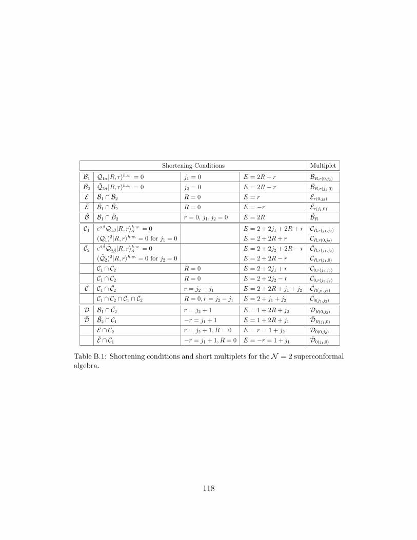
Shortening Conditions Multiplet
B1 Q1α|R, r⟩h.w. = 0 j1 = 0 E = 2R + r BR,r(0,j2)
B2 Q2α|R, r⟩h.w. = 0 j2 = 0 E = 2R− r BR,r(j1,0)
E B1 ∩ B2 R = 0 E = r Er(0,j2)E B1 ∩ B2 R = 0 E = −r Er(j1,0)B B1 ∩ B2 r = 0, j1, j2 = 0 E = 2R BR
C1 ϵαβQ1β|R, r⟩h.w.α = 0 E = 2 + 2j1 + 2R + r CR,r(j1,j2)
(Q1)2|R, r⟩h.w. = 0 for j1 = 0 E = 2 + 2R + r CR,r(0,j2)
C2 ϵαβQ2β|R, r⟩h.w.α = 0 E = 2 + 2j2 + 2R− r CR,r(j1,j2)
(Q2)2|R, r⟩h.w. = 0 for j2 = 0 E = 2 + 2R− r CR,r(j1,0)
C1 ∩ C2 R = 0 E = 2 + 2j1 + r C0,r(j1,j2)C1 ∩ C2 R = 0 E = 2 + 2j2 − r C0,r(j1,j2)
C C1 ∩ C2 r = j2 − j1 E = 2 + 2R + j1 + j2 CR(j1,j2)
C1 ∩ C2 ∩ C1 ∩ C2 R = 0, r = j2 − j1 E = 2 + j1 + j2 C0(j1,j2)D B1 ∩ C2 r = j2 + 1 E = 1 + 2R + j2 DR(0,j2)
D B2 ∩ C1 −r = j1 + 1 E = 1 + 2R + j1 DR(j1,0)
E ∩ C2 r = j2 + 1, R = 0 E = r = 1 + j2 D0(0,j2)
E ∩ C1 −r = j1 + 1, R = 0 E = −r = 1 + j1 D0(j1,0)
Table B.1: Shortening conditions and short multiplets for the N = 2 superconformalalgebra.
118
up to equivalence relations that set to zero all sequences of short multiplets thatmay in principle recombine into long multiplets. The recombination rules for N = 2superconformal algebra are [149]
A2R+r+2j1+2R,r(j1,j2)
≃ CR,r(j1,j2) ⊕ CR+ 12 ,r+
12 (j1−
12 ,j2)
, (B.25)
A2R−r+2j2+2R,r(j1,j2)
≃ CR,r(j1,j2) ⊕ CR+ 12 ,r−
12 (j1,j2−
12 ), (B.26)
A2R+j1+j2+2R,j1−j2(j1,j2)
≃ CR(j1,j2) ⊕ CR+ 12 (j1−
12 ,j2)
⊕ CR+ 12 (j1,j2−
12 )
⊕ CR+1(j1− 12 ,j2−
12 ).
(B.27)
The C, C and C multiplets obey certain “semi-shortening” conditions, while Amultiplets are generic long multiplets. A long multiplet whose conformal dimensionis exactly at the unitarity threshold can be decomposed into shorter multipletsaccording to (B.25, B.26, B.27). We can formally regard any multiplet obeying someshortening condition (with the exception of the E (E) types, and D0(j1,0) (D0(0,j2))
types) as a multiplet of type C, C or C by allowing the spins j1 and j2, whose naturalrange is over the non-negative half-integers, to take the value −1/2 as well. Thetranslation is as follows:
CR,r(− 12,j2)
≃ BR+ 12,r+ 1
2(0,j2)
, CR,r(j1,− 12) ≃ BR+ 1
2,r− 1
2(j1,0)
, (B.28)
CR(− 12,j2)
≃ DR+ 12(0,j2)
, CR(j1,− 12) ≃ DR+ 1
2(j1,0)
, (B.29)
CR(− 12,− 1
2) ≃ DR+ 1
2(0,− 1
2) ≃ DR+ 1
2(− 1
2,0) ≃ BR+1 . (B.30)
Note how these rules flip statistics: a multiplet with bosonic primary (j1 + j2 inte-ger) is turned into a multiplet with fermionic primary (j1 + j2 half-odd), and viceversa. With these conventions, the rules (B.25, B.26, B.27) are the most generalrecombination rules. The E and E multiplets never recombine.
The index of the C and E type multiplets vanishes identically (the choice ofsupercharge with respect to which the index is computed, Q = Q1−, breaks thesymmetry between C (E) and C (E) multiplets). The index of all remaining shortmultiplets can be specified by listing the index of C, C , E , D0(0,j2), and D0(j1,0)
multiplets,
119
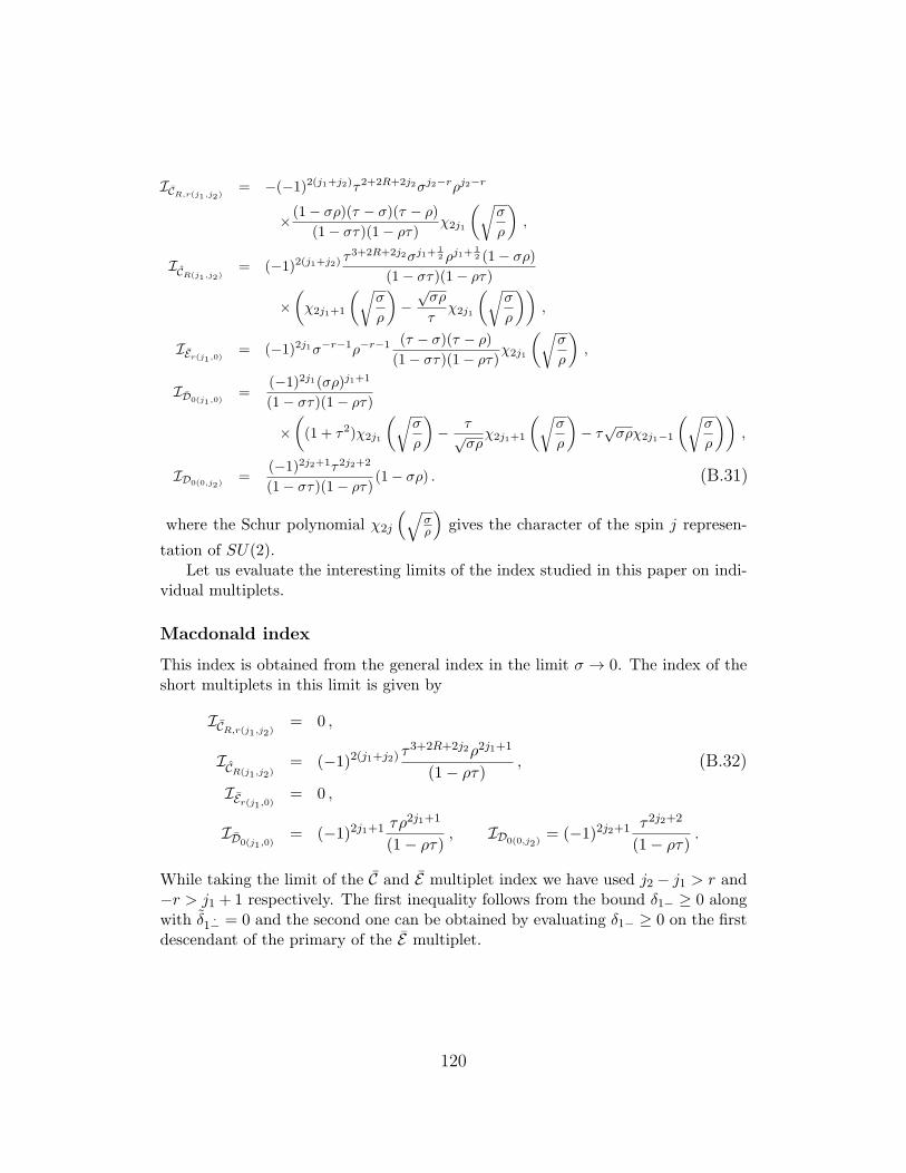
ICR,r(j1,j2)= −(−1)2(j1+j2)τ2+2R+2j2σj2−rρj2−r
× (1− σρ)(τ − σ)(τ − ρ)
(1− στ)(1− ρτ)χ2j1
(√σ
ρ
),
ICR(j1,j2)= (−1)2(j1+j2)
τ3+2R+2j2σj1+12 ρj1+
12 (1− σρ)
(1− στ)(1− ρτ)
×(χ2j1+1
(√σ
ρ
)−
√σρ
τχ2j1
(√σ
ρ
)),
IEr(j1,0)= (−1)2j1σ−r−1ρ−r−1 (τ − σ)(τ − ρ)
(1− στ)(1− ρτ)χ2j1
(√σ
ρ
),
ID0(j1,0)=
(−1)2j1(σρ)j1+1
(1− στ)(1− ρτ)
×((1 + τ2)χ2j1
(√σ
ρ
)− τ
√σρχ2j1+1
(√σ
ρ
)− τ
√σρχ2j1−1
(√σ
ρ
)),
ID0(0,j2)=
(−1)2j2+1τ2j2+2
(1− στ)(1− ρτ)(1− σρ) . (B.31)
where the Schur polynomial χ2j
(√σρ
)gives the character of the spin j represen-
tation of SU(2).Let us evaluate the interesting limits of the index studied in this paper on indi-
vidual multiplets.
Macdonald index
This index is obtained from the general index in the limit σ → 0. The index of theshort multiplets in this limit is given by
ICR,r(j1,j2)= 0 ,
ICR(j1,j2)= (−1)2(j1+j2) τ
3+2R+2j2ρ2j1+1
(1− ρτ), (B.32)
IEr(j1,0) = 0 ,
ID0(j1,0)= (−1)2j1+1 τρ
2j1+1
(1− ρτ), ID0(0,j2)
= (−1)2j2+1 τ2j2+2
(1− ρτ).
While taking the limit of the C and E multiplet index we have used j2 − j1 > r and−r > j1 + 1 respectively. The first inequality follows from the bound δ1− ≥ 0 alongwith δ1− = 0 and the second one can be obtained by evaluating δ1− ≥ 0 on the firstdescendant of the primary of the E multiplet.
120
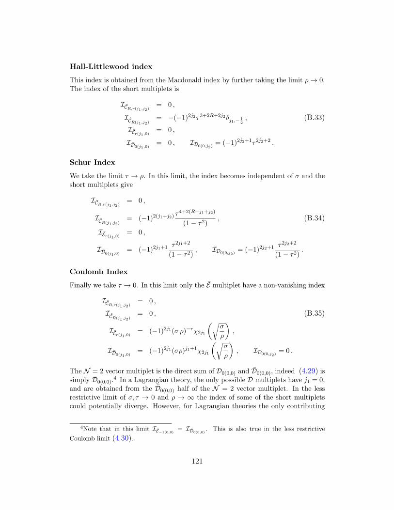
Hall-Littlewood index
This index is obtained from the Macdonald index by further taking the limit ρ→ 0.The index of the short multiplets is
ICR,r(j1,j2)= 0 ,
ICR(j1,j2)= −(−1)2j2τ3+2R+2j2δj1,− 1
2, (B.33)
IEr(j1,0) = 0 ,
ID0(j1,0)= 0 , ID0(0,j2)
= (−1)2j2+1τ2j2+2 .
Schur Index
We take the limit τ → ρ. In this limit, the index becomes independent of σ and theshort multiplets give
ICR,r(j1,j2)= 0 ,
ICR(j1,j2)= (−1)2(j1+j2) τ
4+2(R+j1+j2)
(1− τ2), (B.34)
IEr(j1,0) = 0 ,
ID0(j1,0)= (−1)2j1+1 τ2j1+2
(1− τ2), ID0(0,j2)
= (−1)2j2+1 τ2j2+2
(1− τ2).
Coulomb Index
Finally we take τ → 0. In this limit only the E multiplet have a non-vanishing index
ICR,r(j1,j2)= 0 ,
ICR(j1,j2)= 0 , (B.35)
IEr(j1,0) = (−1)2j1(σ ρ)−rχ2j1
(√σ
ρ
),
ID0(j1,0)= (−1)2j1(σρ)j1+1χ2j1
(√σ
ρ
), ID0(0,j2)
= 0 .
The N = 2 vector multiplet is the direct sum of D0(0,0) and D0(0,0), indeed (4.29) issimply D0(0,0).
4 In a Lagrangian theory, the only possible D multiplets have j1 = 0,and are obtained from the D0(0,0) half of the N = 2 vector multiplet. In the lessrestrictive limit of σ, τ → 0 and ρ → ∞ the index of some of the short multipletscould potentially diverge. However, for Lagrangian theories the only contributing
4Note that in this limit IE−1(0,0)= ID0(0,0)
. This is also true in the less restrictive
Coulomb limit (4.30).
121
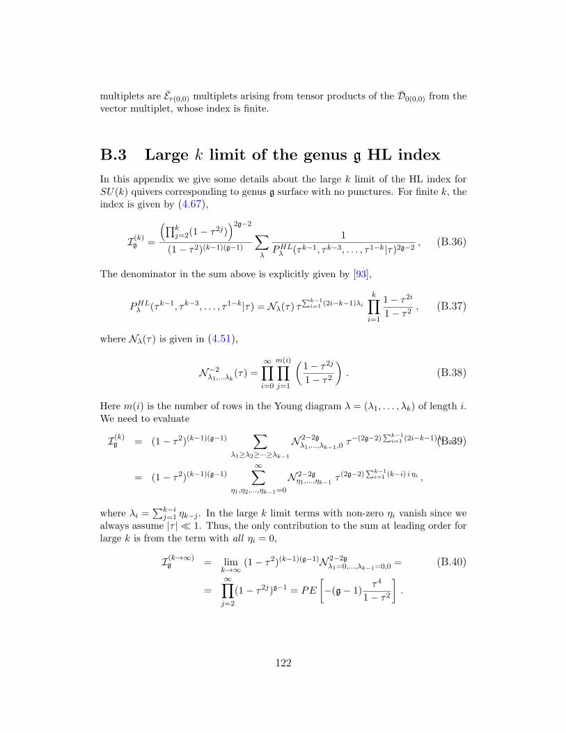
multiplets are Er(0,0) multiplets arising from tensor products of the D0(0,0) from thevector multiplet, whose index is finite.
B.3 Large k limit of the genus g HL index
In this appendix we give some details about the large k limit of the HL index forSU(k) quivers corresponding to genus g surface with no punctures. For finite k, theindex is given by (4.67),
I(k)g =
(∏kj=2(1− τ2j)
)2g−2
(1− τ2)(k−1)(g−1)
∑λ
1
PHLλ (τk−1, τk−3, . . . , τ1−k|τ)2g−2
, (B.36)
The denominator in the sum above is explicitly given by [93],
PHLλ (τk−1, τk−3, . . . , τ1−k|τ) = Nλ(τ) τ
∑k−1i=1 (2i−k−1)λi
k∏i=1
1− τ2i
1− τ2, (B.37)
where Nλ(τ) is given in (4.51),
N−2λ1,...λk
(τ) =∞∏i=0
m(i)∏j=1
(1− τ2j
1− τ2
). (B.38)
Here m(i) is the number of rows in the Young diagram λ = (λ1, . . . , λk) of length i.We need to evaluate
I(k)g = (1− τ2)(k−1)(g−1)
∑λ1≥λ2≥···≥λk−1
N 2−2gλ1,...,λk−1,0
τ−(2g−2)∑k−1
i=1 (2i−k−1)λi =(B.39)
= (1− τ2)(k−1)(g−1)∞∑
η1,η2,...,ηk−1=0
N 2−2gη1,...,ηk−1
τ (2g−2)∑k−1
i=1 (k−i) i ηi ,
where λi =∑k−i
j=1 ηk−j . In the large k limit terms with non-zero ηi vanish since wealways assume |τ | ≪ 1. Thus, the only contribution to the sum at leading order forlarge k is from the term with all ηi = 0,
I(k→∞)g = lim
k→∞(1− τ2)(k−1)(g−1)N 2−2g
λ1=0,...,λk−1=0,0 = (B.40)
=
∞∏j=2
(1− τ2j)g−1 = PE
[−(g− 1)
τ4
1− τ2
].
122
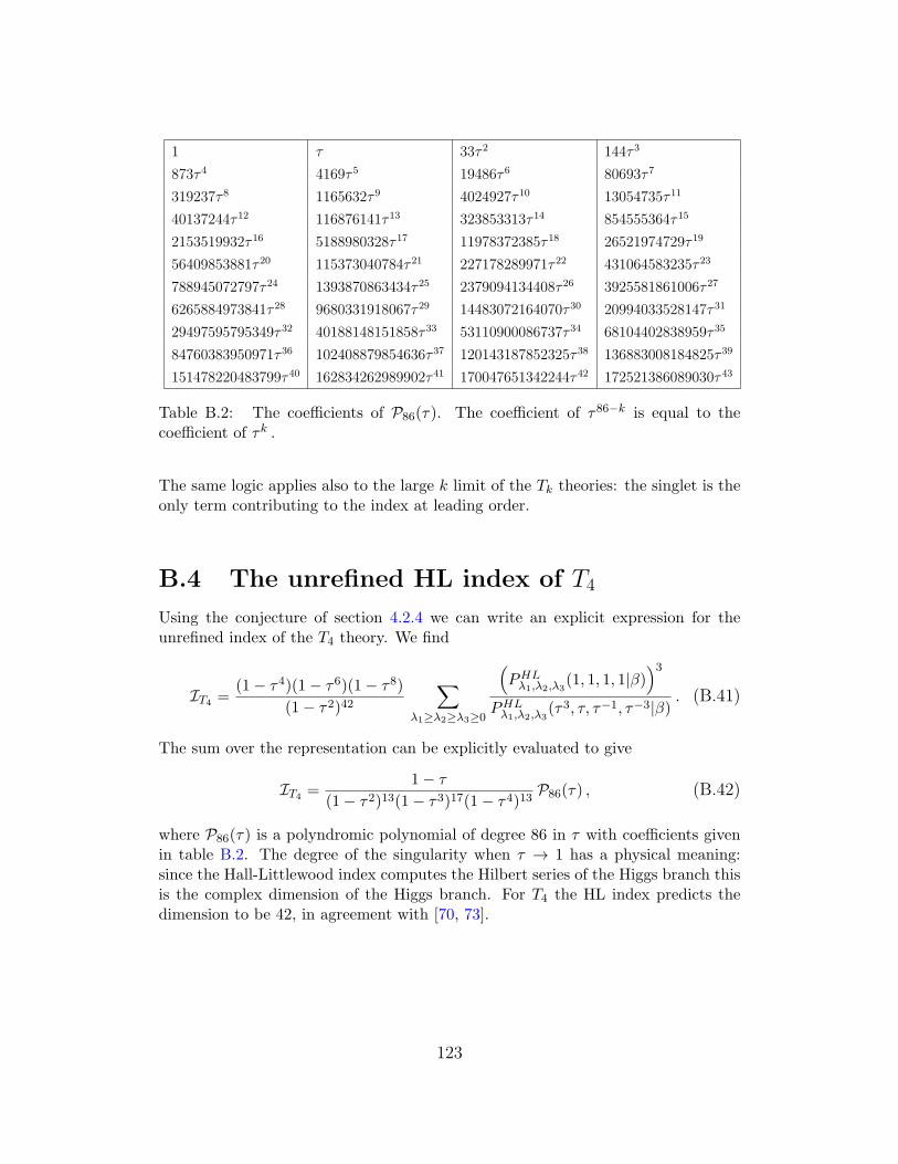
1 τ 33τ 2 144τ 3
873τ 4 4169τ 5 19486τ 6 80693τ 7
319237τ 8 1165632τ 9 4024927τ 10 13054735τ 11
40137244τ 12 116876141τ 13 323853313τ 14 854555364τ 15
2153519932τ 16 5188980328τ 17 11978372385τ 18 26521974729τ 19
56409853881τ 20 115373040784τ 21 227178289971τ 22 431064583235τ 23
788945072797τ 24 1393870863434τ 25 2379094134408τ 26 3925581861006τ 27
6265884973841τ 28 9680331918067τ 29 14483072164070τ 30 20994033528147τ 31
29497595795349τ 32 40188148151858τ 33 53110900086737τ 34 68104402838959τ 35
84760383950971τ 36 102408879854636τ 37 120143187852325τ 38 136883008184825τ 39
151478220483799τ 40 162834262989902τ 41 170047651342244τ 42 172521386089030τ 43
Table B.2: The coefficients of P86(τ). The coefficient of τ86−k is equal to thecoefficient of τk .
The same logic applies also to the large k limit of the Tk theories: the singlet is theonly term contributing to the index at leading order.
B.4 The unrefined HL index of T4
Using the conjecture of section 4.2.4 we can write an explicit expression for theunrefined index of the T4 theory. We find
IT4 =(1− τ4)(1− τ6)(1− τ8)
(1− τ2)42
∑λ1≥λ2≥λ3≥0
(PHLλ1,λ2,λ3
(1, 1, 1, 1|β))3
PHLλ1,λ2,λ3
(τ3, τ, τ−1, τ−3|β). (B.41)
The sum over the representation can be explicitly evaluated to give
IT4 =1− τ
(1− τ2)13(1− τ3)17(1− τ4)13P86(τ) , (B.42)
where P86(τ) is a polyndromic polynomial of degree 86 in τ with coefficients givenin table B.2. The degree of the singularity when τ → 1 has a physical meaning:since the Hall-Littlewood index computes the Hilbert series of the Higgs branch thisis the complex dimension of the Higgs branch. For T4 the HL index predicts thedimension to be 42, in agreement with [70, 73].
123
B.5 Proof of the SU(2) Schur index identity
In this appendix we prove the basic SU(2) Schur index identity (4.93),
PE[q1/2
1−q (a1 +1a1)(a2 +
1a2)(a3 +
1a3)]ai,q
(q; q)3(q2; q)∏3
i=1 PE[
q1−q (a
2i + a−2
i + 2)]ai,q
=∞∑λ=0
∏3i=1 χλ(ai, a
−1i )
χλ(q12 , q−
12 )
.(B.43)
The strategy is to study the analytic properties of this expression and show thatthe left- and right-handed sides have the same poles and residues. Let us first define
x =a1a2a3
, y =a2a1a3
, z =a3a2a1
, u = a1a2a3, xyzu = 1 , (B.44)
where ai are SU(2) fugacities. We also define
(a) ≡ (a; q)∞ ≡∞∏i=0
(1− aqi) . (B.45)
We will use square brackets [ ] to denote ordinary brackets (that delimit expressions).Then, using
∞∑n=1
xn
n= − log(1− x) , (B.46)
the LHS of (B.43) is given by
LHS =[1− q](q)2(qxy)(qxz)(qxu)(qyz)(qyu)(qzu)
(q1/2x)(q1/2/x)(q1/2y)(q1/2/y)(q1/2z)(q1/2/z)(q1/2u)(q1/2/u). (B.47)
Let us study the analytic properties of this expression as a function of x (the ex-pression is symmetric in x, y, z, u). We have poles whenever x = q1/2−l with integerl (positive, zero or negative). At x → 0, ∞ we have accumulation of poles. Let usfor concreteness compute the residue with positive l
ResLHS =[1− q](q)2(q3/2−ly)(q3/2−lz)(q/(yz))(qyz)(q1/2+l/z)(q1/2+l/y)
(q1−l)′(ql)(q1/2y)(q1/2/y)(q1/2z)(q1/2/z)(ql/(yz))(q1−lyz).(B.48)
Here (q1−l)′ is (q1/2x) evaluated at x = q1/2−l with the vanishing factor removed.Now we have
(q1/2−l+1y)(q1/2+l/y)
(q1/2y)(q1/2/y)=
[−y]l
ql2/21
1− q1/2−ly. (B.49)
124
From here we get
ResLHS =[1− q](q)2[yz]l
∏l−2i=0(1− q1+i/(yz))
(q1−l)′(ql)ql2 [1− q1/2−ly][1− q1/2−lz]∏l−1
i=0(1− q−iyz)=q−1/2 − q1/2
A,
(B.50)
where
A = x− 1
x+ y − 1
y+ z − 1
z+ u− 1
u. (B.51)
Let us now look on the RHS of (B.43), which can be written as
RHS =q−1/2 − q1/2
A
∞∑n=1
qn/2
1− qn(xn − 1
xn+ yn − 1
yn+ zn − 1
zn+ un − 1
un) .
(B.52)
We again want to compute residues in x. To see the poles we write
∞∑i=1
qn/2
1− qnxn =
∞∑i=0
∞∑n=1
qn(1/2+i) xn =∞∑i=0
q1/2+i x
1− q1/2+i x. (B.53)
Thus again the poles are at x = q1/2−l for any integer l (we have also same expressionas (B.53) with x→ 1/x). The residue here is easily computed to give
ResRHS =q−1/2 − q1/2
A. (B.54)
All in all, the LHS and RHS have the same poles and residues.
125
Appendix C
Refinement of 3d partitionfunction
The superconformal index defined in section 2.1 is a function of fugacities t, y andv. In order to recover the matrix model of Kapustin et al. [33, 40] in section 5.1we simply fixed the v → t and y → 1. In this appendix we refine the 3d partitionfunction by keeping track of all the fugacities in the index. It is convenient to definethe chemical potentials
v = e−β(1/3+u), y = e−βη. (C.1)
The index, in terms of β, u and η becomes
I = Tr(−1)F e−β[ 23(E+j2)− 1
3(r+R)−(r+R)u+2j1η]. (C.2)
Let us compute the partition function of the hypermultiplet after turning on onlyu.
Ihyp =∏i
Γ
(t2√vai; t
3y, t3y−1
)=∏i
∏n>1
([n+ 1
2 + u2 + iαi]q
[n− 12 − u
2 − iαi]q
)n
q→1−→∏i
[coshπ
(αi − i
u
2
)]− 12
Ivector =∏i<j
1
1− q−i(αi−αj)
1
1− qi(αi−αj)
Γ(q1+u±i(αi−αj); q, q)
Γ(q±i(αi−αj); q, q)
q→1−→∏i<j
(sinhπ(αi − αj)
π(αi − αj)
)2( coshπ(∓(αi − αj) + i/2)
coshπ(∓(αi − αj) + i(u+ 1/2))
)1/2
.
(C.3)
Both partition functions reduce to the ones in section 5.1 as we set u to zero.Now we restore y = q−βη to produce the more refined 3d partition function. The
126
chemical potential η has a nice physical interpretation as the U(1)×U(1) isometrypreserving squashing deformation of the S3. The partition function of 3d gaugetheories on this squashed background was computed in [57].
The contribution due to the hypermultiplet with η deformation turned on is
Ihyp =∏i
Γ(t2√vai; t
3y, t3/y)
y→q−βη
−→∏i
Γ(q1/2−u/2−iαi ; q1+η, q1−η)
=∏i
∏j,k>0
1− q3/2+u/2+iαiq(1+η)jq(1−η)k
1− q1/2−u/2−iαiq(1+η)jq(1−η)k.
(C.4)
Using the regularized infinite product representation of Barnes’ double-Gamma func-tion
Γ2(x|ϵ1, ϵ2) ∝∏
m,n>0
(x+mϵ1 + nϵ2)−1, (C.5)
the partition function of hyper-multiplet can be written in a compact way
Ihyper →∏i
Γ2(1/2− u/2− iαi|1 + η, 1− η)
Γ2(3/2 + u/2 + iαi|1 + η, 1− η)
=∏i
Γ2(Q2 (1/2− u/2)− iαi|b, b−1)
Γ2(Q2 (3/2 + u/2) + iαi|b, b−1)
,
(C.6)
where we have defined1
αi =αi√1− η2
, b =
√1− η
1 + η, Q = b+ b−1. (C.7)
With this change of variables it is easy to see that for u = 0, our result is inagreement with [57]. The partition function of the vector multiplet:
Ivector →∏i<j
1
1− q−i(αi−αj)
1
1− qi(αi−αj)
Γ(q1+u±i(αi−αj); q1+η, q1−η)
Γ(q±i(αi−αj); q1+η, q1−η). (C.8)
1We thank Davide Gaiotto for pointing out this change of variables.
127
reduces to
Ivector =∏i<j
(1− η2) sinhπ(αi−αj)
1+η sinhπ(αi−αj)
1−η
π2(αi − αj)2Γ2(1 + u± i(αi − αj)|1 + η, 1− η)
Γ2(1− u± i(αi − αj)|1 + η, 1− η)
=∏i<j
sinhπb(αi − αj) sinhπb−1(αi − αj)
π2(αi − αj)2Γ2(
Q2 (1 + u)± i(αi − αj)|b, b−1)
Γ2(Q2 (1− u)± i(αi − αj)|b, b−1)
.
(C.9)
Again, we find a precise agreement with the partition function of the vector multipleton squashed S3.
128
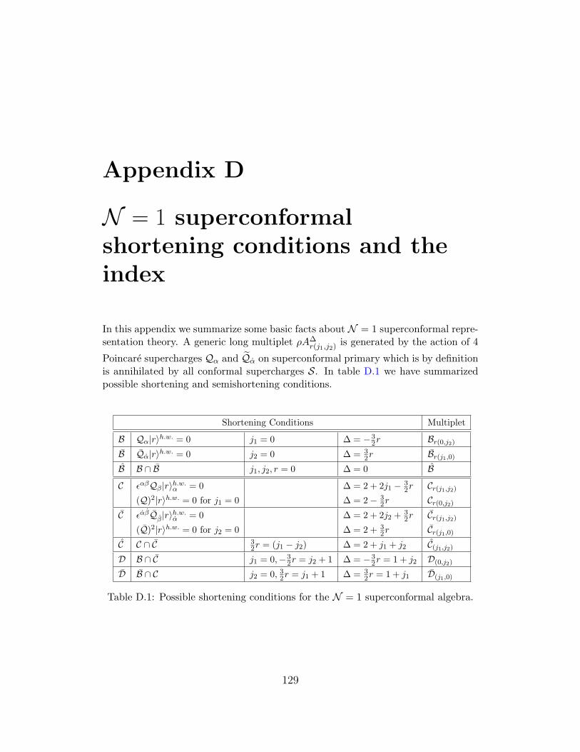
Appendix D
N = 1 superconformalshortening conditions and theindex
In this appendix we summarize some basic facts about N = 1 superconformal repre-sentation theory. A generic long multiplet ρA∆
r(j1,j2)is generated by the action of 4
Poincare supercharges Qα and Qα on superconformal primary which is by definitionis annihilated by all conformal supercharges S. In table D.1 we have summarizedpossible shortening and semishortening conditions.
Shortening Conditions Multiplet
B Qα|r⟩h.w. = 0 j1 = 0 ∆ = −32r Br(0,j2)
B Qα|r⟩h.w. = 0 j2 = 0 ∆ = 32r Br(j1,0)
B B ∩ B j1, j2, r = 0 ∆ = 0 B
C ϵαβQβ|r⟩h.w.α = 0 ∆ = 2 + 2j1 − 3
2r Cr(j1,j2)(Q)2|r⟩h.w. = 0 for j1 = 0 ∆ = 2− 3
2r Cr(0,j2)C ϵαβQβ|r⟩
h.w.α = 0 ∆ = 2 + 2j2 +
32r Cr(j1,j2)
(Q)2|r⟩h.w. = 0 for j2 = 0 ∆ = 2 + 32r Cr(j1,0)
C C ∩ C 32r = (j1 − j2) ∆ = 2 + j1 + j2 C(j1,j2)
D B ∩ C j1 = 0,−32r = j2 + 1 ∆ = −3
2r = 1 + j2 D(0,j2)
D B ∩ C j2 = 0, 32r = j1 + 1 ∆ = 32r = 1 + j1 D(j1,0)
Table D.1: Possible shortening conditions for the N = 1 superconformal algebra.
129
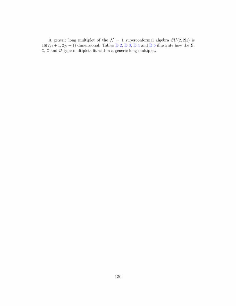
A generic long multiplet of the N = 1 superconformal algebra SU(2, 2|1) is16(2j1 +1, 2j2 +1) dimensional. Tables D.2, D.3, D.4 and D.5 illustrate how the B,C, C and D-type multiplets fit within a generic long multiplet.
130
∆ (j1, j2)
∆ + 12
(j1 + 12, j2) (j1, j2 +
1
2)
(j1 − 12, j2) (j1, j2 −
1
2)
(j1 + 12, j2 + 1
2)
∆ + 1 (j1, j2) (j1 − 12, j2 + 1
2), (j1 + 1
2, j2 − 1
2) (j1, j2)
(j1 − 12, j2 − 1
2)
∆ + 32
(j1, j2 + 12) (j1 + 1
2, j2)
(j1, j2 − 12) (j1 − 1
2, j2)
∆ + 2 (j1, j2)
r − 2 r − 1 r r + 1 r + 2
Table D.2: A long multiplet of N = 1 superconformal algebra. The SU(2, 2) multi-plets that are boxed form a short Br(0,j2) multiplet for j1 = 0,∆ = −3
2r. The left-handed B can be obtained by reflecting the table (that is, sending r → −r and j1 ↔j2). In general, when j1(j2) = 0, the SU(2, 2) multiplets (j1− 1
2 , any)((any, j2−12))
are set to zero, resulting in further shortening.
∆ (j1, j2)
∆ + 12
(j1 +1
2, j2) (j1, j2 +
1
2)
(j1 − 12, j2) (j1, j2 −
1
2)
(j1 +1
2, j2 +
1
2)
∆ + 1 (j1, j2) (j1 − 12, j2 + 1
2) (j1 +
1
2, j2 −
1
2) (j1, j2)
(j1 − 12, j2 − 1
2)
∆ + 32
(j1, j2 + 12) (j1 +
1
2, j2)
(j1, j2 − 12) (j1 − 1
2, j2)
∆ + 2 (j1, j2)
r − 2 r − 1 r r + 1 r + 2
Table D.3: A long multiplet of N = 1 superconformal algebra. The SU(2, 2)multiplets that are boxed form a semi-short Cr(j1,j2) multiplet for ∆ = 2+ 2j1 − 3
2r.The left-handed C can be obtained by reflecting the table (that is, sending r →−r and j1 ↔ j2). In general, when j1(j2) = 0, the SU(2, 2) multiplets (j1 −12 , any)((any, j2 −
12)) are set to zero, resulting in further shortening.
131
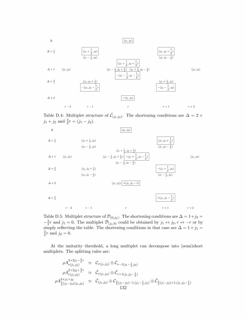
∆ (j1, j2)
∆ + 12
(j1 +1
2, j2) (j1, j2 +
1
2)
(j1 − 12, j2) (j1, j2 − 1
2)
(j1 +1
2, j2 +
1
2)
∆ + 1 (j1, j2) (j1 − 12, j2 + 1
2) (j1 + 1
2, j2 − 1
2) (j1, j2)
−(j1 −1
2, j2 −
1
2)
∆ + 32
(j1, j2 + 12) (j1 + 1
2, j2)
−(j1, j2 −1
2) −(j1 −
1
2, j2)
∆ + 2 −(j1, j2)
r − 2 r − 1 r r + 1 r + 2
Table D.4: Multiplet structure of C(j1,j2). The shortening conditions are ∆ = 2 +
j1 + j2 and 32r = (j1 − j2).
∆ (j1, j2)
∆ + 12
(j1 + 12, j2) (j1, j2 +
1
2)
(j1 − 12, j2) (j1, j2 − 1
2)
(j1 + 12, j2 + 1
2)
∆ + 1 (j1, j2) (j1 − 12, j2 + 1
2), −(j1 +
1
2, j2 −
1
2) (j1, j2)
(j1 − 12, j2 − 1
2)
∆ + 32
(j1, j2 + 12) −(j1 +
1
2, j2)
(j1, j2 − 12) (j1 − 1
2, j2)
∆ + 2 (j1, j2), +(j1, j2 − 1)
∆ + 52
+(j1, j2 −1
2)
r − 2 r − 1 r r + 1 r + 2
Table D.5: Multiplet structure of D(0,j2). The shortening conditions are ∆ = 1+j2 =
−32r and j1 = 0. The multiplet D(j1,0) could be obtained by j1 ↔ j2, r ↔ −r or by
simply reflecting the table. The shortening conditions in that case are ∆ = 1+ j1 =32r and j2 = 0.
At the unitarity threshold, a long multiplet can decompose into (semi)shortmultiplets. The splitting rules are:
ρA2+2j1− 3
2r
r(j1,j2)≃ Cr(j1,j2) ⊕ Cr−1(j1− 1
2,j2)
ρA2+2j2+
32r
r(j1,j2)≃ Cr(j1,j2) ⊕ Cr+1(j1,j2− 1
2)
ρA2+j1+j223(j1−j2)(j1,j2)
≃ C(j1,j2) ⊕ C 23(j1−j2)−1,(j1− 1
2,j2)
⊕ C 23(j1−j2)+1,(j1,j2− 1
2)
132
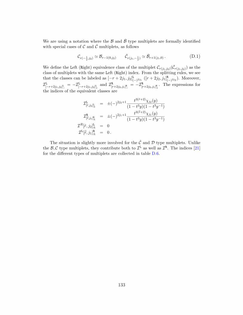
We are using a notation where the B and B type multiplets are formally identifiedwith special cases of C and C multiplets, as follows
Cr(− 12,j2)
≃ Br−1(0,j2) Cr(j1,− 12) ≃ Br+1(j1,0) . (D.1)
We define the Left (Right) equivalence class of the multiplet Cr(j1,j2)(Cr(j1,j2)) as theclass of multiplets with the same Left (Right) index. From the splitting rules, we seethat the classes can be labeled as [−r + 2j1, j2]
L(−)2j1
([r + 2j2, j1]R(−)2j2
). Moreover,
IL[−r+2j1,j2]L−
= −IL[−r+2j1,j2]L+
and IR[r+2j2,j1]R−
= −IR[r+2j2,j1]R+
. The expressions for
the indices of the equivalent classes are
IL[r,j2]L±
= ±(−)2j2+1 t3(r+2)χj2(y)
(1− t3y)(1− t3y−1)
IR[¯r,j1]R±
= ±(−)2j1+1 t3(¯r+2)χj1(y)
(1− t3y)(1− t3y−1)
IR[r, j2]L± = 0
IL[¯r, j1]R± = 0 .
The situation is slightly more involved for the C and D type multiplets. Unlikethe B, C type multiplets, they contribute both to IL as well as IR. The indices [21]for the different types of multiplets are collected in table D.6.
133
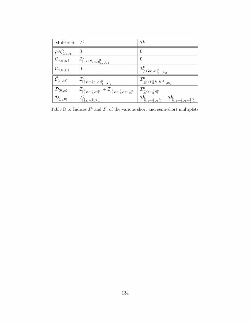
Multiplet IL IR
ρA∆r(j1,j2)
0 0
Cr(j1,j2) IL[−r+2j1,j2]L
(−)2j1
0
Cr(j1,j2) 0 IR[r+2j2,j1]R
(−)2j2
C(j1,j2) IL[ 23j2+
43j1,j2]L
(−)2j1
IR[ 23j1+
43j2,j1]R
(−)2j2
D(0,j2) IL[ 23j2− 4
3,j2]L−
+ IL[ 23j2− 1
3,j2− 1
2]L−
IR[ 43j2− 2
3,0]R+
D(j1,0) IL[ 43j1− 2
3,0]L+
IR[ 23j1− 4
3,j1]R−
+ IR[ 23j1− 1
3,j1− 1
2]R−
Table D.6: Indices IL and IR of the various short and semi-short multiplets.
134
Bibliography
[1] S. Benvenuti, S. Franco, A. Hanany, D. Martelli, and J. Sparks, Aninfinite family of superconformal quiver gauge theories withSasaki-Einstein duals, JHEP 06 (2005) 064, [hep-th/0411264].
[2] J. Kinney, J. M. Maldacena, S. Minwalla, and S. Raju, An index for 4dimensional super conformal theories, Commun. Math. Phys. 275(2007) 209–254, [hep-th/0510251].
[3] D. Gaiotto, N=2 dualities, arXiv:0904.2715.
[4] D. Gaiotto, G. W. Moore, and A. Neitzke, Wall-crossing, HitchinSystems, and the WKB Approximation, arXiv:0907.3987.
[5] S. Cecotti and C. Vafa, Classification of complete N=2 supersymmetrictheories in 4 dimensions, arXiv:1103.5832.
[6] S. Cecotti, A. Neitzke, and C. Vafa, R-Twisting and 4d/2dCorrespondences, arXiv:1006.3435.
[7] M. Alim, S. Cecotti, C. Cordova, S. Espahbodi, A. Rastogi, et al., BPSQuivers and Spectra of Complete N=2 Quantum Field Theories,arXiv:1109.4941.
[8] M. T. Anderson, C. Beem, N. Bobev, and L. Rastelli, HolographicUniformization, arXiv:1109.3724.
[9] L. F. Alday, D. Gaiotto, and Y. Tachikawa, Liouville CorrelationFunctions from Four-dimensional Gauge Theories, Lett. Math. Phys.91 (2010) 167–197, [arXiv:0906.3219].
[10] N. Wyllard, AN−1 conformal Toda field theory correlation functionsfrom conformal N=2 SU(N) quiver gauge theories, JHEP 11 (2009)002, [arXiv:0907.2189].
135
[11] A. Mironov and A. Morozov, On AGT relation in the case of U(3),Nucl.Phys. B825 (2010) 1–37, [arXiv:0908.2569].
[12] N. A. Nekrasov, Seiberg-Witten Prepotential From Instanton Counting,Adv. Theor. Math. Phys. 7 (2004) 831–864, [hep-th/0206161].
[13] V. Pestun, Localization of gauge theory on a four-sphere andsupersymmetric Wilson loops, Commun.Math.Phys. 313 (2012) 71–129,[arXiv:0712.2824].
[14] C. Romelsberger, Counting chiral primaries in N = 1, d=4superconformal field theories, Nucl. Phys. B747 (2006) 329–353,[hep-th/0510060].
[15] A. Gadde, E. Pomoni, L. Rastelli, and S. S. Razamat, S-duality and 2dTopological QFT, JHEP 03 (2010) 032, [arXiv:0910.2225].
[16] A. Gadde, L. Rastelli, S. S. Razamat, and W. Yan, The SuperconformalIndex of the E6 SCFT, JHEP 08 (2010) 107, [arXiv:1003.4244].
[17] A. Gadde, L. Rastelli, S. S. Razamat, and W. Yan, The 4dSuperconformal Index from q-deformed 2d Yang-Mills,arXiv:1104.3850.
[18] A. Gadde, L. Rastelli, S. S. Razamat, and W. Yan, Gauge Theoriesand Macdonald Polynomials, arXiv:1110.3740.
[19] C. Romelsberger, Calculating the Superconformal Index and SeibergDuality, arXiv:0707.3702.
[20] G. Festuccia and N. Seiberg, Rigid Supersymmetric Theories in CurvedSuperspace, JHEP 1106 (2011) 114, [arXiv:1105.0689].
[21] F. A. Dolan and H. Osborn, Applications of the Superconformal Indexfor Protected Operators and q-Hypergeometric Identities to N=1 DualTheories, Nucl. Phys. B818 (2009) 137–178, [arXiv:0801.4947].
[22] V. P. Spiridonov and G. S. Vartanov, Superconformal indices forN = 1 theories with multiple duals, Nucl. Phys. B824 (2010) 192–216,[arXiv:0811.1909].
[23] V. P. Spiridonov and G. S. Vartanov, Elliptic hypergeometry ofsupersymmetric dualities, arXiv:0910.5944.
136
[24] V. Spiridonov and G. Vartanov, Supersymmetric dualities beyond theconformal window, Phys.Rev.Lett. 105 (2010) 061603,[arXiv:1003.6109].
[25] A. Gadde, L. Rastelli, S. S. Razamat, and W. Yan, On theSuperconformal Index of N=1 IR Fixed Points: A Holographic Check,JHEP 1103 (2011) 041, [arXiv:1011.5278].
[26] G. Vartanov, On the ISS model of dynamical SUSY breaking,arXiv:1009.2153.
[27] V. Spiridonov and G. Vartanov, Elliptic hypergeometry ofsupersymmetric dualities II. Orthogonal groups, knots, and vortices,arXiv:1107.5788.
[28] P. C. Argyres and N. Seiberg, S-duality in n=2 supersymmetric gaugetheories, JHEP 0712 (2007) 088.
[29] J. A. Minahan and D. Nemeschansky, An N = 2 superconformal fixedpoint with E(6) global symmetry, Nucl. Phys. B482 (1996) 142–152,[hep-th/9608047].
[30] I. R. Klebanov and E. Witten, Superconformal field theory onthree-branes at a Calabi-Yau singularity, Nucl.Phys. B536 (1998)199–218, [hep-th/9807080].
[31] M. Cvetic, H. Lu, D. N. Page, and C. Pope, New Einstein-Sasakispaces in five and higher dimensions, Phys.Rev.Lett. 95 (2005) 071101,[hep-th/0504225].
[32] Y. Nakayama, Index for supergravity on AdS(5) x T**1,1 and conifoldgauge theory, Nucl.Phys. B755 (2006) 295–312, [hep-th/0602284].
[33] A. Kapustin, B. Willett, and I. Yaakov, Nonperturbative Tests ofThree-Dimensional Dualities, JHEP 10 (2010) 013, [arXiv:1003.5694].
[34] A. Kapustin, B. Willett, and I. Yaakov, Tests of Seiberg-like Duality inThree Dimensions, arXiv:1012.4021.
[35] N. Drukker, M. Marino, and P. Putrov, From weak to strong couplingin ABJM theory, arXiv:1007.3837.
[36] C. P. Herzog, I. R. Klebanov, S. S. Pufu, and T. Tesileanu,Multi-Matrix Models and Tri-Sasaki Einstein Spaces, Phys. Rev. D83(2011) 046001, [arXiv:1011.5487].
137
[37] D. L. Jafferis, The Exact Superconformal R-Symmetry Extremizes Z,arXiv:1012.3210.
[38] D. Martelli and J. Sparks, The large N limit of quiver matrix modelsand Sasaki- Einstein manifolds, arXiv:1102.5289.
[39] D. L. Jafferis, I. R. Klebanov, S. S. Pufu, and B. R. Safdi, Towards theF-Theorem: N=2 Field Theories on the Three- Sphere, JHEP 06(2011) 102, [arXiv:1103.1181].
[40] A. Kapustin, B. Willett, and I. Yaakov, Exact Results for Wilson Loopsin Superconformal Chern- Simons Theories with Matter, JHEP 03(2010) 089, [arXiv:0909.4559].
[41] V. Spiridonov, Elliptic hypergeometric functions, arXiv:0704.3099.
[42] A. Gadde, E. Pomoni, and L. Rastelli, The Veneziano Limit of N=2Superconformal QCD: Towards the String Dual of N = 2SU(Nc) SYMwith Nf = 2Nc, arXiv:0912.4918.
[43] K. A. Intriligator and B. Wecht, The Exact superconformal R symmetrymaximizes a, Nucl.Phys. B667 (2003) 183–200, [hep-th/0304128].
[44] O. Aharony, J. Marsano, S. Minwalla, K. Papadodimas, andM. Van Raamsdonk, A first order deconfinement transition in large NYang- Mills theory on a small 3-sphere, Phys. Rev. D71 (2005) 125018,[hep-th/0502149].
[45] O. Aharony, J. Marsano, and M. Van Raamsdonk, Two loop partitionfunction for large N pure Yang-Mills theory on a small S**3, Phys.Rev. D74 (2006) 105012, [hep-th/0608156].
[46] M. Mussel and R. Yacoby, The 2-loop partition function of large Ngauge theories with adjoint matter on S3, JHEP 12 (2009) 005,[arXiv:0909.0407].
[47] G. Ishiki, Y. Takayama, and A. Tsuchiya, N = 4 SYM on R x S**3 andtheories with 16 supercharges, JHEP 10 (2006) 007, [hep-th/0605163].
[48] E. Witten, Constraints on Supersymmetry Breaking, Nucl.Phys. B202(1982) 253.
[49] B. Feng, A. Hanany, and Y.-H. He, Counting Gauge Invariants: thePlethystic Program, JHEP 03 (2007) 090, [hep-th/0701063].
138
[50] S. Benvenuti, B. Feng, A. Hanany, and Y.-H. He, Counting BPSoperators in gauge theories: Quivers, syzygies and plethystics, JHEP 11(2007) 050, [hep-th/0608050].
[51] O. Aharony, J. Marsano, S. Minwalla, K. Papadodimas, andM. Van Raamsdonk, The Hagedorn / deconfinement phase transition inweakly coupled large N gauge theories, Adv. Theor. Math. Phys. 8(2004) 603–696, [hep-th/0310285].
[52] F. Benini, Y. Tachikawa, and B. Wecht, Sicilian gauge theories andN=1 dualities, arXiv:0909.1327.
[53] Y. Tachikawa and B. Wecht, Explanation of the Central Charge Ratio27/32 in Four- Dimensional Renormalization Group Flows betweenSuperconformal Theories, Phys. Rev. Lett. 103 (2009) 061601,[arXiv:0906.0965].
[54] J. van Diejen and V. Spiridonov, Elliptic Beta Integrals and MudularHypergeometric Sums: An Overview, Rocky Mountain J. Math. 32 (2)(2002) 639–656.
[55] V. Spiridonov, Essays on the theory of elliptic hypergeometric functions,Uspekhi Mat. Nauk 63 no 3 (2008) 3–72, [arXiv:0805.3135].
[56] V. Spiridonov, Classical elliptic hypergeometric functions and theirapplications , Rokko Lect. in Math. Vol. 18, Dept. of Math, Kobe Univ.(2005) 253–287, [math/0511579].
[57] N. Hama, K. Hosomichi, and S. Lee, SUSY Gauge Theories onSquashed Three-Spheres, JHEP 05 (2011) 014, [arXiv:1102.4716].
[58] E. Witten, Geometric Langlands From Six Dimensions,arXiv:0905.2720.
[59] N. Drukker, D. R. Morrison, and T. Okuda, Loop operators andS-duality from curves on Riemann surfaces, JHEP 09 (2009) 031,[arXiv:0907.2593].
[60] N. Drukker, J. Gomis, T. Okuda, and J. Teschner, Gauge Theory LoopOperators and Liouville Theory, JHEP 02 (2010) 057,[arXiv:0909.1105].
[61] L. F. Alday, D. Gaiotto, S. Gukov, Y. Tachikawa, and H. Verlinde,Loop and surface operators in N=2 gauge theory and Liouville modulargeometry, JHEP 01 (2010) 113, [arXiv:0909.0945].
139
[62] A. Mironov and A. Morozov, Proving AGT relations in the large-climit, Phys. Lett. B682 (2009) 118–124, [arXiv:0909.3531].
[63] L. F. Alday, F. Benini, and Y. Tachikawa, Liouville/Toda centralcharges from M5-branes, arXiv:0909.4776.
[64] R. Poghossian, Recursion relations in CFT and N=2 SYM theory,JHEP 12 (2009) 038, [arXiv:0909.3412].
[65] A. Marshakov, A. Mironov, and A. Morozov, On non-conformal limitof the AGT relations, Phys. Lett. B682 (2009) 125–129,[arXiv:0909.2052].
[66] G. Bonelli and A. Tanzini, Hitchin systems, N=2 gauge theories andW-gravity, arXiv:0909.4031.
[67] A. Marshakov, A. Mironov, and A. Morozov, Zamolodchikovasymptotic formula and instanton expansion in N=2 SUSY Nf = 2Nc
QCD, JHEP 11 (2009) 048, [arXiv:0909.3338].
[68] D. V. Nanopoulos and D. Xie, On Crossing Symmmetry and ModularInvariance in Conformal Field Theory and S Duality in Gauge Theory,Phys. Rev. D80 (2009) 105015, [arXiv:0908.4409].
[69] D. Gaiotto, Asymptotically free N=2 theories and irregular conformalblocks, arXiv:0908.0307.
[70] D. Gaiotto and J. Maldacena, The gravity duals of N=2 superconformalfield theories, arXiv:0904.4466.
[71] Y. Tachikawa, Six-dimensional DN theory and four-dimensionalSO-USp quivers, JHEP 07 (2009) 067, [arXiv:0905.4074].
[72] R. Dijkgraaf and C. Vafa, Toda Theories, Matrix Models, TopologicalStrings, and N=2 Gauge Systems, arXiv:0909.2453.
[73] F. Benini, S. Benvenuti, and Y. Tachikawa, Webs of five-branes andN=2 superconformal field theories, JHEP 09 (2009) 052,[arXiv:0906.0359].
[74] K. Maruyoshi, M. Taki, S. Terashima, and F. Yagi, New SeibergDualities from N=2 Dualities, JHEP 09 (2009) 086,[arXiv:0907.2625].
140
[75] D. Nanopoulos and D. Xie, N=2 SU Quiver with USP Ends or SU Endswith Antisymmetric Matter, JHEP 08 (2009) 108, [arXiv:0907.1651].
[76] F. J. van de Bult, An elliptic hypergeometric integral with w(f4)symmetry, arXiv:0909.4793.
[77] P. C. Argyres and J. R. Wittig, Infinite coupling duals of N=2 gaugetheories and new rank 1 superconformal field theories, JHEP 01 (2008)074, [arXiv:0712.2028].
[78] S. O. Spiridonov, V.P. an Warnaar, Inversions of integral operators andelliptic beta integrals on root systems , Adv. Math. 207 (2006) 91–132,[math/0411044].
[79] O. Aharony and Y. Tachikawa, A holographic computation of thecentral charges of d=4, N=2 SCFTs, JHEP 01 (2008) 037,[arXiv:0711.4532].
[80] D. Gaiotto, A. Neitzke, and Y. Tachikawa, Argyres-Seiberg duality andthe Higgs branch, Commun. Math. Phys. 294 (2010) 389–410,[arXiv:0810.4541].
[81] M. Atiyah, Topological quantum field theories, Inst. Hautes Etudes Sci.Publ. Math. 68 (1989) 175–186.
[82] R. Dijkgraaf, Fields, strings and duality, hep-th/9703136.
[83] E. M. Rains, Transformations of Elliptic Hypergeometric Integrals ,math/0309252.
[84] M. R. Gaberdiel and B. Zwiebach, Exceptional groups from openstrings, Nucl. Phys. B518 (1998) 151–172, [hep-th/9709013].
[85] E. Witten, On quantum gauge theories in two-dimensions,Commun.Math.Phys. 141 (1991) 153–209.
[86] E. Witten, Two-dimensional gauge theories revisited, J. Geom. Phys. 9(1992) 303–368, [hep-th/9204083].
[87] S. Cordes, G. W. Moore, and S. Ramgoolam, Lectures on 2-dYang-Mills theory, equivariant cohomology and topological field theories,Nucl. Phys. Proc. Suppl. 41 (1995) 184–244, [hep-th/9411210].
[88] S. Benvenuti, A. Hanany, and N. Mekareeya, The Hilbert Series of theOne Instanton Moduli Space, JHEP 06 (2010) 100, [arXiv:1005.3026].
141
[89] A. Hanany and N. Mekareeya, Tri-vertices and SU(2)’s, JHEP 1102(2011) 069, [arXiv:1012.2119].
[90] J. Gray, A. Hanany, Y.-H. He, V. Jejjala, and N. Mekareeya, SQCD: AGeometric Apercu, JHEP 0805 (2008) 099, [arXiv:0803.4257].
[91] A. Hanany and N. Mekareeya, Counting Gauge Invariant Operators inSQCD with Classical Gauge Groups, JHEP 0810 (2008) 012,[arXiv:0805.3728].
[92] J. A. Minahan and D. Nemeschansky, Superconformal fixed points withE(n) global symmetry, Nucl. Phys. B489 (1997) 24–46,[hep-th/9610076].
[93] I. G. Macdonald, Symmetric functions and hall polynomials, OxfordUniversity Press (1995).
[94] O. Chacaltana and J. Distler, Tinkertoys for Gaiotto Duality, JHEP 11(2010) 099, [arXiv:1008.5203].
[95] G. W. Moore and Y. Tachikawa, On 2d TQFTs whose values areholomorphic symplectic varieties, arXiv:1106.5698.
[96] D. Gaiotto, G. W. Moore, and Y. Tachikawa, On 6d N=(2,0) theorycompactified on a Riemann surface with finite area, arXiv:1110.2657.
[97] Y. Nakayama, Index for orbifold quiver gauge theories, Phys. Lett.B636 (2006) 132–136, [hep-th/0512280].
[98] H. Awata and Y. Yamada, Five-dimensional AGT Conjecture and theDeformed Virasoro Algebra, JHEP 01 (2010) 125, [arXiv:0910.4431].
[99] R. Schiappa and N. Wyllard, An Ar threesome: Matrix models, 2dCFTs and 4d N = 2 gauge theories, arXiv:0911.5337.
[100] A. Mironov, A. Morozov, S. Shakirov, and A. Smirnov, Proving AGTconjecture as HS duality: extension to five dimensions,arXiv:1105.0948.
[101] M. Aganagic, H. Ooguri, N. Saulina, and C. Vafa, Black holes,q-deformed 2d Yang-Mills, and non- perturbative topological strings,Nucl. Phys. B715 (2005) 304–348, [hep-th/0411280].
[102] M. Blau and G. Thompson, Lectures on 2-d gauge theories: Topologicalaspects and path integral techniques, hep-th/9310144.
142
[103] F. A. H. Dolan, V. P. Spiridonov, and G. S. Vartanov, From 4dsuperconformal indices to 3d partition functions, arXiv:1104.1787.
[104] A. Gadde and W. Yan, Reducing the 4d Index to the S3 PartitionFunction, arXiv:1104.2592.
[105] Y. Imamura, Relation between the 4d superconformal index and the S3
partition function, JHEP 1109 (2011) 133, [arXiv:1104.4482].
[106] F. Benini, T. Nishioka, and M. Yamazaki, 4d Index to 3d Index and 2dTQFT, arXiv:1109.0283.
[107] M. Aganagic and S. Shakirov, Knot Homology from RefinedChern-Simons Theory, arXiv:1105.5117.
[108] I. Cherednik, Double Affine Hecke Algebras. Cambridge UniversityPress, 2005.
[109] A. A. Kirillov Jr, Lectures on affine hecke algebras and macdonald’sconjectures, Bull. Amer. Math. Soc. 34 (1997) 251–293.
[110] V. Spiridonov and G. Vartanov, Superconformal indices of N = 4 SYMfield theories, Lett.Math.Phys. 100 (2012) 97–118, [arXiv:1005.4196].
[111] V. Spiridonov, On the elliptic beta function, Russ. Math. Surveys 56(2001) 185.
[112] F. Benini, Y. Tachikawa, and D. Xie, Mirrors of 3d Sicilian theories,JHEP 09 (2010) 063, [arXiv:1007.0992].
[113] S. Benvenuti and S. Pasquetti, 3D-partition functions on the sphere:exact evaluation and mirror symmetry, JHEP 1205 (2012) 099,[arXiv:1105.2551].
[114] T. Nishioka, Y. Tachikawa, and M. Yamazaki, 3d Partition Function asOverlap of Wavefunctions, JHEP 1108 (2011) 003, [arXiv:1105.4390].
[115] M. Yamazaki, Brane Tilings and Their Applications, Fortsch. Phys. 56(2008) 555–686, [arXiv:0803.4474].
[116] B. Feng, A. Hanany, and Y.-H. He, D-brane gauge theories from toricsingularities and toric duality, Nucl. Phys. B595 (2001) 165–200,[hep-th/0003085].
[117] C. E. Beasley and M. R. Plesser, Toric duality is Seiberg duality, JHEP12 (2001) 001, [hep-th/0109053].
143
[118] B. Feng, A. Hanany, Y.-H. He, and A. M. Uranga, Toric duality asSeiberg duality and brane diamonds, JHEP 12 (2001) 035,[hep-th/0109063].
[119] H. Ooguri and C. Vafa, Geometry of N = 1 dualities in fourdimensions, Nucl. Phys. B500 (1997) 62–74, [hep-th/9702180].
[120] F. Cachazo, B. Fiol, K. A. Intriligator, S. Katz, and C. Vafa, Ageometric unification of dualities, Nucl. Phys. B628 (2002) 3–78,[hep-th/0110028].
[121] B. Feng, A. Hanany, and Y.-H. He, Phase structure of D-brane gaugetheories and toric duality, JHEP 08 (2001) 040, [hep-th/0104259].
[122] B. Feng, S. Franco, A. Hanany, and Y.-H. He, Symmetries of toricduality, JHEP 12 (2002) 076, [hep-th/0205144].
[123] S. Franco, A. Hanany, Y.-H. He, and P. Kazakopoulos, Duality walls,duality trees and fractional branes, hep-th/0306092.
[124] A. Dymarsky, I. Klebanov, and R. Roiban, Perturbative gauge theoryand closed string tachyons, JHEP 0511 (2005) 038, [hep-th/0509132].
[125] S. Benvenuti and M. Kruczenski, Semiclassical strings inSasaki-Einstein manifolds and long operators in N = 1 gauge theories,JHEP 10 (2006) 051, [hep-th/0505046].
[126] H. Kihara, M. Sakaguchi, and Y. Yasui, Scalar Laplacian onSasaki-Einstein manifolds Y(p,q), Phys. Lett. B621 (2005) 288–294,[hep-th/0505259].
[127] T. Oota and Y. Yasui, Toric Sasaki-Einstein manifolds and Heunequations, Nucl. Phys. B742 (2006) 275–294, [hep-th/0512124].
[128] S. S. Gubser, Einstein manifolds and conformal field theories, Phys.Rev. D59 (1999) 025006, [hep-th/9807164].
[129] A. Ceresole, G. Dall’Agata, R. D’Auria, and S. Ferrara, Spectrum oftype IIB supergravity on AdS(5) x T(11): Predictions on N = 1SCFT’s, Phys. Rev. D61 (2000) 066001, [hep-th/9905226].
[130] A. Ceresole, G. Dall’Agata, and R. D’Auria, KK spectroscopy of typeIIB supergravity on AdS(5) x T(11), JHEP 11 (1999) 009,[hep-th/9907216].
144
[131] P. I. Etingof and A. A. Kirillov, Jr., On the affine analog of Jack’s andMacDonald’s polynomials, hep-th/9403168.
[132] E. M. Rains, BCn-symmetric abelian functions, math/0402113.
[133] A. Gorsky and N. Nekrasov, Hamiltonian systems of Calogero type andtwo-dimensional Yang-Mills theory, Nucl.Phys. B414 (1994) 213–238,[hep-th/9304047].
[134] J. A. Minahan and A. P. Polychronakos, Interacting fermion systemsfrom two-dimensional QCD, Phys.Lett. B326 (1994) 288–294,[hep-th/9309044].
[135] A. Gorsky and N. Nekrasov, Relativistic Calogero-Moser model asgauged WZW theory, Nucl.Phys. B436 (1995) 582–608,[hep-th/9401017].
[136] A. Gorsky and N. Nekrasov, Elliptic Calogero-Moser system fromtwo-dimensional current algebra, hep-th/9401021.
[137] A. Gorsky, Integrable many-body systems in the field theories,Theoretical and Mathematical Physics 103 (1995) 681–700.
[138] A. Gorsky and A. Mironov, Integrable many body systems and gaugetheories, hep-th/0011197.
[139] A. A. Gerasimov and S. L. Shatashvili, Higgs Bundles, Gauge Theoriesand Quantum Groups, Commun.Math.Phys. 277 (2008) 323–367,[hep-th/0609024].
[140] R. Ruijsenaars, Elliptic integrable systems of Calogero-Moser type: Asurvey, Rokko Lectures in Math no. 18 (2004) 201–221.
[141] N. A. Nekrasov and S. L. Shatashvili, Quantization of IntegrableSystems and Four Dimensional Gauge Theories, arXiv:0908.4052.
[142] N. Nekrasov and E. Witten, The Omega Deformation, Branes,Integrability, and Liouville Theory, JHEP 09 (2010) 092,[arXiv:1002.0888].
[143] V. Spiridonov, Elliptic hypergeometric functions andcalogero-sutherland-type models, Theoretical and Mathematical Physics150 (2007) 266–277. 10.1007/s11232-007-0020-5.
145
[144] V. Spiridonov, Elliptic beta integrals and solvable models of statisticalmechanics, Contemp.Math. 563 (2012) 181–211, [arXiv:1011.3798].
[145] F. A. Dolan, Counting BPS operators in N=4 SYM, Nucl. Phys. B790(2008) 432–464, [arXiv:0704.1038].
[146] R. Slansky, Group Theory for Unified Model Building, Phys. Rept. 79(1981) 1–128.
[147] V. K. Dobrev and V. B. Petkova, All Positive Energy UnitaryIrreducible Representations of Extended Conformal Supersymmetry,Phys. Lett. B162 (1985) 127–132.
[148] V. K. Dobrev and V. B. Petkova, GROUP THEORETICALAPPROACH TO EXTENDED CONFORMAL SUPERSYMMETRY:FUNCTION SPACE REALIZATIONS AND INVARIANTDIFFERENTIAL OPERATORS, Fortschr. Phys. 35 (1987) 537.
[149] F. A. Dolan and H. Osborn, On short and semi-short representationsfor four dimensional superconformal symmetry, Ann. Phys. 307 (2003)41–89, [hep-th/0209056].
146