1

THE UNIVERSITY OF HULL

An acoustic water tank disdrometer

being a Thesis submitted for the Degree of Doctor of Philosophy

in the University of Hull

by

Mr. Philip Newton Winder, MEng

August 2010

2

Abstract

Microwave engineers and geomorphologists require rainfall data with a much greater

temporal resolution and a better representation of the numbers of large raindrops than is

available from current commercial instruments. This Thesis describes the development of an

acoustic instrument that determines rain parameters from the sound of raindrops falling into

a tank of water. It is known as the acoustic water tank disdrometer (AWTD).

There is a direct relationship between the kinetic energy of a raindrop and the acoustic

energy generated upon impact. Rain kinetic energy flux density (KE) is estimated from

measurements of the sound field in the tank and these have been compared to measurements

from a co-sited commercial disdrometer.

Furthermore, using an array of hydrophones it is possible to determine the drop size and

impact position of each raindrop falling into the tank. Accumulating the information from

many impacts allows a drop size distribution (DSD) to be calculated.

Eight months of data have been collected in the Eastern UK. The two methods of parameter

estimation are developed and analysed to show that the acoustic instrument can produce rain

KE measurements with a one-second integration times and DSDs with accurate large drop-

size tails.

3

Acknowledgements

All of my gratitude is owed to colleagues, friends and family who have lent their support over

the past three years. Their commitment and encouragement have guided me towards the

production of this Thesis.

I would like to commend my supervisor, Dr. Kevin Paulson, for the huge amount of effort that

he has invested in me. Without his guidance, patience and work, I would have gained nothing.

I must also thank the staff within the Department of Engineering who, on numerous occasions,

provided me with insight, help, work and coffee!

Friends have always provided an endearing distraction. The memories of the days and nights

spent drinking, eating and discussing ridiculously random topics will undoubtedly fade into a

haze of happiness. However, I have no doubt that the friends that I have met, along with those

who are too stubborn to get rid of me, will provide a source of amusement and enlightenment

for decades to come. I do not have the space to mention everyone, but you all know who you

are anyway. A special thanks goes to Nick Winder and Ben Henson for proofing this Thesis.

My upmost thanks and appreciation goes to both my and Emma’s family, for providing the

love and support that I now, undeservedly, take for granted.

Finally; Em. I cannot possibly write enough to describe everything you have ever done for me.

So, thank you for everything.

Ultimately, the responsibility for this Thesis is mine. However, everyone in my life should take

the credit for many different reasons. If there are areas that are inadequate, it is likely due to

the neglect of their advice.

Thank you all.

4

Table of Contents

Abstract ................................................................................. 2

Acknowledgements ................................................................ 3

Table of Contents ................................................................... 4

Table of Figures ...................................................................... 8

Chapter 1: Introduction ........................................................ 12 1.1 Aims and methodology ............................................................................................................................... 13 1.2 Organisation of the Thesis ......................................................................................................................... 14

Chapter 2: Literature review ................................................. 16

2.1 Meteorological principals .......................................................................................................................... 16 2.1.1 The hydrological cycle ........................................................................................................................ 17

2.1.1.1 Surface tension ......................................................................................................... 17 2.1.1.2 Evaporation ............................................................................................................... 17 2.1.1.3 Atmospheric temperature ........................................................................................ 17 2.1.1.4 Drop formation ......................................................................................................... 18 2.1.1.5 Precipitation .............................................................................................................. 18

2.1.2 The drop size distribution................................................................................................................. 19 2.1.2.1 Applications of the DSD ............................................................................................ 19 2.1.2.2 Marshall-Palmer (M-P) distribution .......................................................................... 20 2.1.2.3 Gamma distribution .................................................................................................. 20 2.1.2.4 Event descriptors ...................................................................................................... 21 2.1.2.5 Rain intensity............................................................................................................. 21

2.2 An impacting drop ........................................................................................................................................ 22 2.2.1 Drop velocity .......................................................................................................................................... 22 2.2.2 Drop kinetic energy ............................................................................................................................. 25 2.2.3 Sound generation .................................................................................................................................. 26

2.2.3.1 Entrainment .............................................................................................................. 28 2.2.3.2 Impact ....................................................................................................................... 29

2.3 An appraisal of current disdrometers .................................................................................................. 30 2.3.1 Joss-Waldvogel ...................................................................................................................................... 31 2.3.2 Thies Clima laser precipitation monitor ..................................................................................... 32 2.3.3 2D Video Disdrometer ........................................................................................................................ 34 2.3.4 Discussion ................................................................................................................................................ 34

2.4 Advances in acoustic disdrometry ......................................................................................................... 34 2.4.1 Total acoustic intensity inversions................................................................................................ 35 2.4.2 Direct inversion from impact pressures ..................................................................................... 37

2.5 Summary ........................................................................................................................................................... 38

Chapter 3: System design ..................................................... 39

3.1 System components ..................................................................................................................................... 40 3.1.1 Hydrophones .......................................................................................................................................... 40

3.1.1.1 A comparison between underwater and air acoustics ............................................. 40 3.1.1.2 Piezoelectric transducers .......................................................................................... 43 3.1.1.3 External impedance mismatches .............................................................................. 44 3.1.1.4 Hydrophone choice ................................................................................................... 45

5

3.1.2 Water tank dimensions ...................................................................................................................... 45 3.1.3 Data acquisition ..................................................................................................................................... 47 3.1.4 Optimal hydrophone placement ..................................................................................................... 50

3.2 Electronics ........................................................................................................................................................ 50 3.2.1 Overview .................................................................................................................................................. 50 3.2.2 Requirements ......................................................................................................................................... 51 3.2.3 Design ........................................................................................................................................................ 52

3.2.3.1 Charge Amplifier ....................................................................................................... 52 3.2.3.2 Power Supply Filtering .............................................................................................. 53 3.2.3.3 Schematic .................................................................................................................. 53

3.2.4 Noise .......................................................................................................................................................... 55 3.2.4.1 Voltage noise ............................................................................................................. 55

3.2.5 Noise verification .................................................................................................................................. 57 3.3 Anechoic lining ............................................................................................................................................... 58

3.3.1 Theory ....................................................................................................................................................... 58 3.3.2 Results ....................................................................................................................................................... 60 3.3.3 Conclusions ............................................................................................................................................. 64

3.4 Summary ........................................................................................................................................................... 64

Chapter 4: Total sound field interpretation ............................ 66 4.1 Comparison of instrument measurements ......................................................................................... 66 4.2 Sampling statistics ........................................................................................................................................ 67

4.2.1 Sample errors in catchment rain measurements .................................................................... 68 4.2.2 Comparison of AWTD and LPM rain kinetic energy flux ...................................................... 69

4.3 Establishing relationships ......................................................................................................................... 70 4.3.1 Rain kinetic energy flux ..................................................................................................................... 70 4.3.2 Rain intensity ......................................................................................................................................... 71 4.3.3 Results ....................................................................................................................................................... 72 4.3.4 Increasing the temporal resolution............................................................................................... 73 4.3.5 The effect of wind ................................................................................................................................. 76

4.4 The relationship with the drop size distribution ............................................................................. 77 4.4.1 Introduction ............................................................................................................................................ 77 4.4.2 Principal component analysis ......................................................................................................... 77 4.4.3 Fitting distributions ............................................................................................................................. 78

4.4.3.1 Results ....................................................................................................................... 79 4.5 Conclusions ...................................................................................................................................................... 80

Chapter 5: Entrainment noise ............................................... 81

5.1 Introduction .................................................................................................................................................... 81 5.2 Liquid alteration ............................................................................................................................................ 82

5.2.1 Applications to the AWTD ................................................................................................................. 82 5.2.2 Experimentation with viscous films ............................................................................................. 83

5.3 Driven oscillation .......................................................................................................................................... 84 5.3.1 Applications to the AWTD ................................................................................................................. 84

5.3.1.1 Initial experimentation ............................................................................................. 84 5.3.2 A model of an oscillating bubble .................................................................................................... 85 5.3.3 Bubble forcing conclusions ............................................................................................................... 87

5.4 Summary ........................................................................................................................................................... 88

Chapter 6: Impact filtering .................................................... 89

6.1 Introduction .................................................................................................................................................... 90 6.1.1 Sources of noise ..................................................................................................................................... 90 6.1.2 A detailed look at an impact signal ................................................................................................ 91

6

6.1.2.1 The frequency components of the impact process .................................................. 91 6.1.2.2 Consequences ........................................................................................................... 92

6.1.3 Discriminating an impact by its shape ......................................................................................... 93 6.1.3.1 Time domain impact-bubble comparison ................................................................. 93

6.2 Advanced filtering techniques ................................................................................................................. 94 6.2.1 Matched filtering ................................................................................................................................... 94

6.2.1.1 Matched filter post-processing ................................................................................. 95 6.2.2 Filtering by power ................................................................................................................................ 96

6.2.2.1 Root-mean-square (RMS) method ............................................................................ 97 6.2.2.2 Hilbert transform method ......................................................................................... 97

6.2.3 Wavelet filtering .................................................................................................................................. 100 6.2.3.1 A wavelet interpretation of an impact and bubble ................................................ 101

6.2.4 Other filtering possibilities ............................................................................................................. 103 6.3 Filter implementation ............................................................................................................................... 103

6.3.1.1 Correlation method ................................................................................................. 104 6.3.1.2 Hilbert method ........................................................................................................ 105 6.3.1.3 Wavelet method ..................................................................................................... 105

6.4 Filter comparison ........................................................................................................................................ 105 6.4.1 Methodology ......................................................................................................................................... 105 6.4.2 Results ..................................................................................................................................................... 106 6.4.3 Discussion .............................................................................................................................................. 107

6.4.3.1 Examples of errors .................................................................................................. 108 6.4.3.2 Hilbert method errors ............................................................................................. 109

6.5 Conclusions .................................................................................................................................................... 110

Chapter 7: Direct interpretation .......................................... 111

7.1 Impact decoding .......................................................................................................................................... 112 7.1.1 Impact dataset acquisition .............................................................................................................. 112 7.1.2 Closer inspection ................................................................................................................................ 114

7.1.2.1 Method.................................................................................................................... 114 7.1.3 Multiple impacts – spatial filtering .............................................................................................. 114

7.1.3.1 Method.................................................................................................................... 114 7.1.4 Impact decoding wrapper ............................................................................................................... 116

7.1.4.1 Method.................................................................................................................... 116 7.2 Impact positioning – multilateration .................................................................................................. 117

7.2.1 Derivation .............................................................................................................................................. 117 7.2.1.1 Standard multilateration equations ........................................................................ 118 7.2.1.2 Multilateration simplification ................................................................................. 119 7.2.1.3 Numerical solution .................................................................................................. 120

7.2.2 Testing ..................................................................................................................................................... 121 7.2.3 Three- and four-hydrophone multilateration algorithms ................................................. 122

7.2.3.1 Three hydrophone multilateration ......................................................................... 122 7.2.3.2 Method.................................................................................................................... 122

7.3 Establishing the drop size ........................................................................................................................ 124 7.3.1 Theoretical drop size approximation ......................................................................................... 124 7.3.2 Experimental drop size approximation ..................................................................................... 125

7.3.2.1 Drop velocity testing ............................................................................................... 125 7.3.2.2 Impact pressure testing .......................................................................................... 126

7.3.3 Application of drop size approximations .................................................................................. 128 7.4 DSD generation ............................................................................................................................................ 128

7.4.1 DSD results and comparison .......................................................................................................... 128

7

7.4.1.1 Individual DSD examples ......................................................................................... 129 7.4.1.2 Temporal DSD data ................................................................................................. 130 7.4.1.3 Time series analysis ................................................................................................. 131

7.4.2 DSD errors ............................................................................................................................................. 132 7.4.2.1 Inherent AWTD errors ............................................................................................. 133

7.5 Summary ......................................................................................................................................................... 134

Chapter 8: Summary and conclusions ................................. 135

8.1 Final summary .............................................................................................................................................. 135 8.2 Further work ................................................................................................................................................. 139

8.2.1 Further additions to the AWTD .................................................................................................... 140 8.2.2 The use of a digital signal processor ........................................................................................... 140 8.2.3 The acoustic metal plate disdrometer ....................................................................................... 141 8.2.4 The acoustic tent disdrometer ...................................................................................................... 141

8.3 Concluding remarks ................................................................................................................................... 142

Appendix ........................................................................... 143

A.1 Hydrophone calibration ........................................................................................................................... 143 A.1.1 Method .................................................................................................................................................... 143

A.2 Multilateration simplification derivation ......................................................................................... 143 A.3 List of publications ..................................................................................................................................... 145

References ......................................................................... 146

8

Table of Figures

Figure 2.1: Computed shapes for d = 1, 2, 3, 4, 5 and 6 mm with origin at centre of mass. Shown for comparison are dashed circles of diameter d divided into 45 degree sectors (from Beard and Chuang (1987) with permission)..................................................................... 23

Figure 2.2: The terminal velocity of raindrops. Lines are models, circles are experimental data. ........................................................................................................................................................................... 24

Figure 2.3: A zoomed version of Figure 2.2 hilighting the difference in accuracy when comparing models. Lines are models, circles are experimental data. ................................. 24

Figure 2.4: A typical measured droplet impact and bubble signal using the AWTD. .................... 28

Figure 2.5: The Joss-Waldvogel Impact disdrometer (courtesy of Distromet Ltd.)....................... 31

Figure 2.6: The Thies Clima Laser Precipitation Monitor (LPM) (courtesy of Thies Clima) ...... 32

Figure 2.7: The required Thies Clima LPM bit rate for various rain intensities. ............................. 33

Figure 2.8: The 2D Video Disdrometer (courtesy of Kruger and Krajewski (2002)) .................... 34

Figure 3.1: The experimental acoustic water tank disdrometer. PC and electronics located elsewhere for protection. ....................................................................................................................... 40

Figure 3.2: Microscopic permutations are the cause of the piezoelectric effect. When a molecular structure is at equilibrium, a), the net dipole moment is zero. When the structure is deformed, b), the dipole moment changes by p. .................................................. 43

Figure 3.3: The net result of applying an electric field. At rest, a), the net charge zero, hence the material is in equilibrium. When an electric potential is applied, b), the material deforms due to the polarisation of the domains. .......................................................................... 43

Figure 3.4: An image depicting the dipole effect on hydrophone placement. .................................. 46

Figure 3.5: The relative loss due to the dipole effect against an increasing hydrophone spacing. ........................................................................................................................................................................... 47

Figure 3.6: The errors due to sampling. Image a) describes the error associated with two hydrophones (large dots) on the same axis. The TOAs from the two hydrophones form two circles representing the possible impact locations (spaced dots). In the worse case, one hydrophone circle would be +0.36 mm away from the real impact location (star) and the other hydrophone circle would be -0.36 mm away. The area formed by the intersecting circles is the error area. Image b) is an emphasised version of a). ...... 48

Figure 3.7: Definitions to calculate the error area. ...................................................................................... 48

Figure 3.8: The sampling error with respect to hydrophone placement. 100% error is determined at the point where the hydrophones are touching (±1 cm). ........................... 49

Figure 3.9: The combination of the dipole and sampling errors to yield a minimum error which occurs at approximately ±0.1 m from the centre of the tank. ................................... 50

Figure 3.10: A component level model of a hydrophone. Bottom: internal, top: external. ......... 51

Figure 3.11: A stylised frequency response of a hydrophone. ................................................................ 51

Figure 3.12: An operational amplifier in a charge amplifier configuration. ..................................... 52

Figure 3.13: A schematic of the AWTD pre-amplifier ................................................................................ 54

Figure 3.14: Charge amplifier noise analysis. ................................................................................................ 55

9

Figure 3.15: A random example 1 second worth of raw pre-amplifier data, filtered between 1 and 50 kHz. ................................................................................................................................................... 58

Figure 3.16: Charge amplifier noise analysis. ................................................................................................ 59

Figure 3.17: Transmission coefficient for a 1cm slab of: a) rubber, and b) aluminium, in water. ........................................................................................................................................................................... 61

Figure 3.18: Predicted loss factor using the parameters from Ouis (2005). .................................... 62

Figure 3.19: Loss factor based upon real data. a) Undamped, b) damped with 1cm thick rubber sheet ................................................................................................................................................................ 63

Figure 3.20: Full AWTD hardware schematic ................................................................................................ 64

Figure 4.1: Comparison of LPM derived raindrop kinetic energy flux density with total acoustic energy integrated over one minute. The error bars indicate uncertainty due to sampling errors. Both the KE flux density and the total acoustic pressure are normalised to a catchment of 1 m2 over an integration time of 1 hour. ............................. 70

Figure 4.2: Comparison of LPM derived rain intensity with total acoustic energy integrated over one minute. ........................................................................................................................................ 72

Figure 4.3: An example rain event comparing the measured KE between the LPM (grey) and AWTD (black). ............................................................................................................................................. 72

Figure 4.4: An example rain event comparing the measured RI between the LPM (grey) and AWTD (black). ............................................................................................................................................. 73

Figure 4.5: Kinetic energy flux density time series derived from AWTD data, (grey) with a 10 second integration time compared to LPM data (black) with a 60 second integration time. ................................................................................................................................................................. 74

Figure 4.6: Rain intensity time series derived from AWTD data, (grey) with a 10 second integration time compared to LPM data (black) with a 60 second integration time. ... 74

Figure 4.7: Kinetic energy flux density time series derived from AWTD data, (grey) with a 1 second integration time compared to LPM data (black) with a 60 second integration time. ................................................................................................................................................................. 75

Figure 4.8: Rain intensity time series derived from AWTD data, (grey) with a 1 second integration time compared to LPM data (black) with a 60 second integration time. ... 75

Figure 4.9: The new KE-AWTD relationship after compensating for the lack of a horizontal wind reading from LPM. Stars indicate the data recorded with the highest average wind speeds. ................................................................................................................................................ 76

Figure 4.10: An example DSD reconstruction from three principal components. ......................... 78

Figure 4.11: An example DSD and distribution fitting (black = measured DSD, grey = gamma, dash = exponential). ................................................................................................................................. 79

Figure 4.12: Fitting the total AI to gamma and exponential distributions. a) The LPM measured DSD, b) an artificial fit using a gamma distribution and c) an artificial fit using an exponential distribution. The exponential fits poorly. The gamma fits well (averaged correlation coefficient of 0.90). ............................................................................................................ 79

Figure 5.1: Testing the performance of an oil layer. a) Control, water only, b) 1 cm thick oil layer added. .................................................................................................................................................. 83

Figure 5.2: The bubble forcing experimental result reproduced with a logarithmic y scale. The addition of a forcing signal (red) is compared to the original, non-forced, signal (black) in the frequency domain. The addition of a forcing signal has little effect at the bubbles’ frequencies................................................................................................................................. 85

10

Figure 5.3: A numerical solution to a modified version of equation (5.2), simulating bubble creation and oscillation. a) the driving impulse (i.e. crater collapse and initial compression) and b) the resulting bubble oscillation, in terms of R. .................................. 86

Figure 5.4: Simulating bubble formation and oscillation when exposed to a driving sound field. As Figure 5.3. ............................................................................................................................................... 87

Figure 5.5: The normalised frequency spectrum of Figure 5.3 b) (solid line) and Figure 5.4 b) (dashed line). ............................................................................................................................................... 87

Figure 6.1: A short time fast Fourier transform of an impact and bubble. ........................................ 92

Figure 6.2: A zoomed version of Figure 6.1 (impact) ................................................................................. 92

Figure 6.3: A zoomed version of Figure 6.1 (bubble) ................................................................................. 92

Figure 6.4: An ideal impact and bubble signal. ............................................................................................. 93

Figure 6.5: Using the matched filter method on an example impact and bubble signal. a) Correlation coefficient set to 0.7. b) Correlation coefficient set to 0.9. c) Matched filter post-processing applied. Potential impacts are black asterisks. ........................................... 95

Figure 6.6: An example calculation of the RMS pressure of a bubble (black = bubble signal, blue = 2 samples, red = 12 samples, green = 24 samples, yellow = 120 samples). ........ 97

Figure 6.7: An example showing the application of the discrete Hilbert transform (black) to a bubble (a) and an impact (b) (both in grey). .................................................................................. 98

Figure 6.8: Using the Hilbert filter method on an example impact and bubble signal. ................ 99

Figure 6.9: The discrete Mayer wavelet function. The scaling function averages the decomposition provided by the wavelet function to encourage accurate results without an infinite temporal resolution......................................................................................... 101

Figure 6.10: Example wavelet decompositions using different wavelet functions (x-scale = time (ms), y-scale = amplitude (Pa)). .............................................................................................. 101

Figure 6.11: A zoomed version of the discrete Meyer plot of Figure 6.10. ...................................... 102

Figure 6.12: Output from wavelet detection routine for an example impact and bubble. a) and b) are zoomed images of the impacts at 16 and 275 ms, respectively. ............................. 103

Figure 6.13: Algorithms for the various impact filtering methods. .................................................... 104

Figure 6.14: Example of possible filtering errors due to: a) noise, b) impact in bubble, c) bubble that looks like impact (stars denote possible error locations, raw data in grey). ......................................................................................................................................................................... 108

Figure 6.15: An example of the Hilbert transform method of filtering. The frequent threshold crossing of the envelope results in small RMS amplitudes and false potential impacts. (Raw data = grey, envelope = black, threshold = black dash). .............................................. 109

Figure 7.1: Impact dataset acquisition. .......................................................................................................... 112

Figure 7.2: Closer inspection algorithm. ........................................................................................................ 114

Figure 7.3: An algorithm to use spatial filtering to decide which combination of impact pulses is most likely to represent an impact. ............................................................................................. 115

Figure 7.4: DSD generation algorithm wrapper. ........................................................................................ 116

Figure 7.5: Depiction of the time difference of arrival (TDOA). ........................................................... 118

Figure 7.6: A solution to known y coordinates. .......................................................................................... 120

Figure 7.7: A solution to the multilateration routines using iteration and Aitken’s acceleration. ......................................................................................................................................................................... 121

11

Figure 7.8: Testing the multilateration routines. Crosses are solutions to a dataset, stars are the locations of hydrophones and the line is the tank boundary. ....................................... 122

Figure 7.9: A zoomed-in version of Figure 7.8. ........................................................................................... 122

Figure 7.10: Three- and four-hydrophone versions of the multilateration algorithms. ............ 123

Figure 7.11: Plotting the impact velocity vs. pressure. Points are individual impacts from heights between 0.5 and 2.5m. The line is the least-squares best fit which shows that the pressure is proportional to the velocity to a power of 2.86, which is in agreement with published results. .......................................................................................................................... 126

Figure 7.12: Results from the pressure-to-drop size calibration exercise. Points are individual impacts taken from LPM and raw AWTD data and fitted with least-squares regression. ......................................................................................................................................................................... 127

Figure 7.13: Drop normalisation and sizing routine. ............................................................................... 128

Figure 7.14: The averaged DSDs from the LPM (black) and the AWTD (red) with associated standard errors for each bin (shading). ......................................................................................... 129

Figure 7.15: A selection of DSDs from the LPM (black) and the AWTD (red). ............................... 130

Figure 7.16: A plot of the LPM (a) and AWTD (b) DSDs vs. time where the z-axis is the drop frequency per m2 per minute. The smallest discernable drop threshold for the AWTD data (b) is shown as a white line in (a). .......................................................................................... 130

Figure 7.17: Temporal exponential shape (μ) parameter comparison of all drop diameters. Black = LPM, red = AWTD. ................................................................................................................... 132

Figure 7.18: Temporal exponential scale parameter comparison of drop diameters greater than 1.8 mm. Black = LPM, red = AWTD. ....................................................................................... 132

12

Chapter 1: Introduction

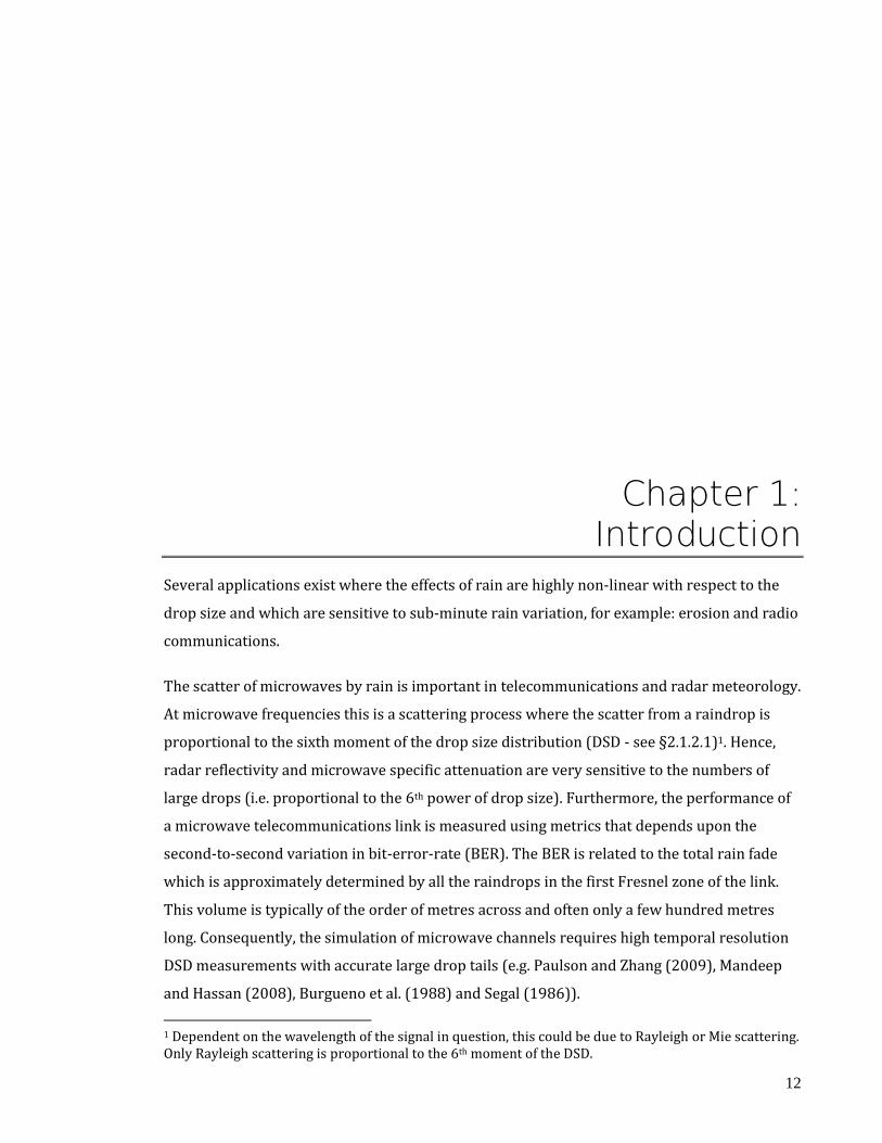
Several applications exist where the effects of rain are highly non-linear with respect to the

drop size and which are sensitive to sub-minute rain variation, for example: erosion and radio

communications.

The scatter of microwaves by rain is important in telecommunications and radar meteorology.

At microwave frequencies this is a scattering process where the scatter from a raindrop is

proportional to the sixth moment of the drop size distribution (DSD - see §2.1.2.1)1. Hence,

radar reflectivity and microwave specific attenuation are very sensitive to the numbers of

large drops (i.e. proportional to the 6th power of drop size). Furthermore, the performance of

a microwave telecommunications link is measured using metrics that depends upon the

second-to-second variation in bit-error-rate (BER). The BER is related to the total rain fade

which is approximately determined by all the raindrops in the first Fresnel zone of the link.

This volume is typically of the order of metres across and often only a few hundred metres

long. Consequently, the simulation of microwave channels requires high temporal resolution

DSD measurements with accurate large drop tails (e.g. Paulson and Zhang (2009), Mandeep

and Hassan (2008), Burgueno et al. (1988) and Segal (1986)).

1 Dependent on the wavelength of the signal in question, this could be due to Rayleigh or Mie scattering. Only Rayleigh scattering is proportional to the 6th moment of the DSD.

13

Similarly, erosion processes are sensitive to rapid rain variation and are highly non-linear in

drop size (Van Dijk et al. (2002)). Erosivity is a combined function of the rain intensity and of

its velocity, so rain kinetic energy flux is often cited as a primary indicator, e.g. Brodie and

Rosewell (2007), Salles and Poesen (2000). A large proportion of the kinetic energy is carried

by the small proportion of larger drops. Hence, accurately determining the number of larger

drops over small timescales is of great importance to geomorphologists.

Meteorology and communications converge when a mutual necessity for new models and data

are required to increase efficiency and understand fundamental physical phenomena. By

designing a system that is able to represent the proportion of large drops within a rain event,

or by measuring their cumulative effects, more stable communications links or better erosion

predictions would be possible.

1.1 Aims and methodology The raindrop arrival rate is approximated to a scaled exponential distribution with respect to

drop size, when averaged over a long period (§2.1.2.2). I.e. large drops will occur less often

than smaller drops. Many current disdrometers (e.g. Thies Clima laser precipitation monitor,

Joss-Waldvogel impact disdrometer - §2.3) use a small catchment area to reduce the

possibility of two simultaneous impacts appearing like a single large one. This reduces the

chances of the disdrometer observing a large sized drop and therefore reduces the validity of

the result that it produces (i.e. increases the variance). As a compromise, these disdrometers

perform measurements of a period of one minute (or longer), which gives the disdrometer a

good chance of seeing a few large drops. Furthermore, decreasing the size of the catchment

area also reduces the dead-time; the time in which an instrument cannot perform

measurements after an event due to mechanical or electrical constraints.

To improve the temporal resolution and to measure the large drop tail of the DSD more

accurately, a larger catchment area is required. One potential method that has been

investigated in the past is to use a body of water as the catchment (§2.4). This could

potentially yield catchment areas many orders of magnitude larger than current disdrometers

and hence, results and temporal resolutions many orders of magnitude more reliable and

higher, respectively.

There are two potential areas of development. The first is the development of a device that is

similar to previous works (§2.4) which uses part of the total sound generated by a rain event.

Previous authors have aimed to use this method at sea due to the potentially huge catchment

14

areas, although the background noise would be inherently high. However, they have only used

these methods at long integration times using empirical conversion factors. This project will

investigate the use of all the available data (i.e. all of the total sound field) and at temporal

resolutions much greater than other disdrometers.

The second field of study is much more novel. By using an array of hydrophones at the bottom

of the tank it is possible to individually pick out individual drops as they impact on the tank’s

surface, even if they occur at a similar time to other drops. Mani and Pillai (2004) have

published a similar method, but with limited success (see §2.4.2). After correctly establishing

the impact, position and drop size, an accurate representation of the DSD should be possible.

1.2 Organisation of the Thesis This Thesis represents the progression and culmination of the acoustic water tank

disdrometer (AWTD) project. Chapters 1 and 2 contain a discussion regarding the previous

study of the effects and phenomena of rain. These chapters stress potential problems that

could be encountered and formulate goals for the project to attain. The middle chapters, 3-7

contain the development and results of the project. The details of chapters 2-8 are outlined

below.

Chapter 2 introduces the topic of meteorology pertaining to the process of rain formation and

precipitation. Several metrics critical to the measurement of rain are introduced along with a

review of the phenomena of an impacting drop. A critique of several comparable commercial

disdrometers is performed whilst highlighting areas for improvement. Finally, recent research

regarding acoustic disdrometry is reviewed and potential research areas established.

The third chapter details the design and construction of the disdrometer. It discusses the

hardware requirements including the electronic amplification, data acquisition, hydrophones

and the anechoic properties required to increase the performance of the direct interpretation

method (Chapter 7).

Chapter 4 describes the first successful method of rain interpretation. It details the

methodology, performance and results of using the total sound field of the impact process to

generate rain intensity (RI), kinetic energy (KE) flux density and DSD information. This part of

the project greatly improves upon the specifications of other disdrometers by reducing the

temporal resolution of the data to 1 s intervals.

15

With chapter 5 begins the second phase of the project. It investigates all possible sources of

noise and establishes that the noise produced from the entrainment process is likely to be the

largest source of error. Two methods of entrainment suppression are presented with limited

success.

Chapter 6 investigates the use of software methods to correctly determine whether a signal is

an impact or a drop. One method in particular proved to be successful by systematically

analysing and testing each method.

Chapter 7 describes the culmination of the second phase of the project which generates a DSD

from the sounds of individual impacts. The impact filtering of Chapter 6 is combined with

decoding and positioning algorithms to invert the impact sounds intro drop sizes using an

empirical relationship. Averaged results show a good fit to the LPM, but temporal analysis

reveals some short term variation which degrades instantaneous DSDs.

Finally, chapter 8 summarises the entire work and poses ideas and questions for further work.

An overall conclusion of the project is also provided.

16

Chapter 2: Literature review

This chapter presents experiments and theories regarding the process of rain generation and

precipitation, with an emphasis on measurement. Several descriptors of rain are introduced

including the drop size distribution and rain intensity. Parameters that affect an impacting

drop are examined with the intention of introducing the sound generation process. A critique

of current commercial disdrometers is presented highlighting areas of potential

improvement. Finally, recent research into the field of acoustic disdrometry is reviewed,

advances are investigated and further research areas are established.

2.1 Meteorological principals Meteorology is a vast multi-disciplinary subject that focuses on measuring or predicting the

weather. The acoustic disdrometer fits securely within the measuring domain, but we still

need to consider the hydrological processes that create the phenomena we are attempting to

measure. First, we consider the physical micro-processes and explain how precipitation forms

and falls. Then the concept of a drop size distribution is introduced along with the different

effects of drop size.

17

2.1.1 The hydrological cycle The hydrological cycle is defined as the method of water and water vapour transport around

the earth. It is unnecessary to detail all aspects, but the fundamentals, principally relating to

the formation and precipitation of rain, are reviewed here.

2.1.1.1 Surface tension

Consider an interface between a body of water and the air above. If we imagine that we are

able to observe the water molecules travelling in a random motion it would be possible to see

that some molecules are travelling faster than others. Some molecules will undergo speed

changes through collisions. On approaching the surface, molecules will appear to be repelled

and reversed as if a force was opposing their trajectory, (Cole (1975)).

If molecules are within close proximity, it disturbs their surface charge distribution in such a

way that weak electrical attraction forces are established. Molecules upon the surface are

subjected to a force in a direction towards the body of water, since they are bound by their

mutual attractions and attractions with molecules below the surface. A surface force, or

tension, is set up which acts at a normal to the surface. Since molecules are attracted to each

other, there is a tendency for the surface area to become as small as possible. The ideal case is

seen in the form of a spherical rain drop in the lower 10 to 15 km of the troposphere, (Cole

(1975)).

2.1.1.2 Evaporation

The surface tension of a liquid poses a barrier that makes molecular escape, or evaporation,

through the surface difficult. Hence, molecules are only able to overcome the surface tension

when they have enough kinetic energy and their average motion is directed outward from the

surface. The rate of evaporation therefore depends on the number of molecules that have

enough kinetic energy to escape. The eventual quantity of molecules in the air, or water

vapour, depends on the difference between the kinetic energy of the departing molecules and

the average kinetic energy of those left behind, (Cole (1975)). The air is considered to be

saturated when the rate at which water vapour enters the water equals that of the water

molecules entering the air. This is known as the saturation vapour pressure; a quantity that

depends on temperature, (H.Riehl (1978)).

2.1.1.3 Atmospheric temperature

Temperature is defined by the energy held by vibrating atoms. A greater vibration yields the

increased ability to transfer some of that energy to other molecules; as humans, we feel this as

heat. A volume of air must support the column of air above it. This leads to exponential decay

18

with altitude of pressure and density of each gas species. Most of the radiant heat from the

sun passes through the atmosphere and warms the surface of the Earth, while a fraction is

reflected back into space. This heat is dissipated from the surface by re-radiation at lower

frequencies, conduction and convection. Equilibrium is reached when the radiant energy

reaching the Earth is balanced by the energy re-radiated. These processes lead to a

temperature gradient with altitude which has an average lapse rate of 6.5 degrees per

kilometre (Ahrens (2008)).

2.1.1.4 Drop formation

The principal factor causing condensation is the cooling of the water vapour as the warm air

rises in altitude. Section 2.1.1.2 established that only a certain amount of water vapour can

sustain itself before it begins to reform in a liquid state, known as the dew point. However, at

elevations above the surface of the earth, the temperature frequently falls well below the dew

point, without condensation taking place. The Bergeron process (Lutgens and Tarbuck

(1998)) indicates that pure saturated air can be cooled to approximately -40°C (or -40°F)

without condensation occurring and water droplets at these temperatures are said to be in a

supercooled state. Below this temperature the molecules can spontaneously form ice crystals

(Cole (1975)).

However, the presence of particles within the atmosphere provides a surface for condensation

to occur; these are known as condensation nuclei. There are two types of nuclei: hygroscopic,

which are usually ionic salts and are able to cause condensation in non-saturated air, and

hydrophobic which require saturated conditions. The condensation rate of a single drop will

continue to decrease until the equilibrium conditions similar to §2.1.1.2 occur. However, and

additional process is the growth of raindrops by collision and coalescence. A drop may collide,

coalesce and increase its mass. Its combined velocity will increase and collide with more

drops at a faster rate; precipitation will follow. Unlike condensation, the rate at which this

process occurs will increase non-linearly (Wells (1997)).

2.1.1.5 Precipitation

Small sized hydrometeors can appear to float in the air as clouds, when in fact they are being

directed by pockets of moving air (i.e. winds). Coalescence will occur until the hydrometeors

are heavy enough to start falling back towards the ground. In certain storms, formed at the

threshold of two opposing weather fronts, the underlying air and the hydrometeors contained

within can get pushed back upwards towards the cloud. When this happens repeated cycles of

coalescence and precipitation can occur. In such cases, the hydrometeors can become

19

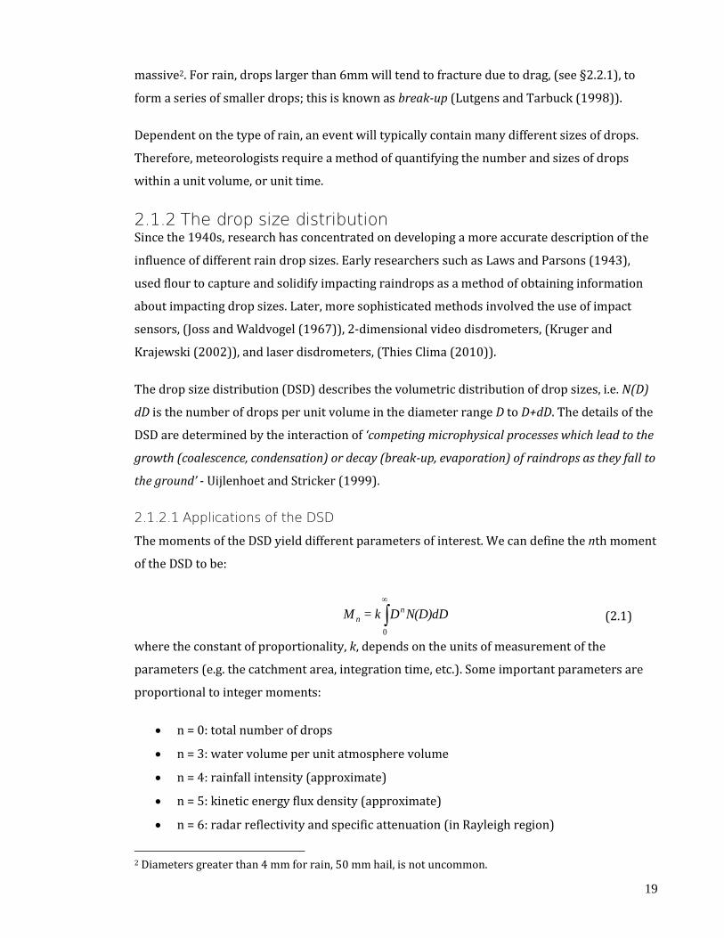
massive2. For rain, drops larger than 6mm will tend to fracture due to drag, (see §2.2.1), to

form a series of smaller drops; this is known as break-up (Lutgens and Tarbuck (1998)).

Dependent on the type of rain, an event will typically contain many different sizes of drops.

Therefore, meteorologists require a method of quantifying the number and sizes of drops

within a unit volume, or unit time.

2.1.2 The drop size distribution Since the 1940s, research has concentrated on developing a more accurate description of the

influence of different rain drop sizes. Early researchers such as Laws and Parsons (1943),

used flour to capture and solidify impacting raindrops as a method of obtaining information

about impacting drop sizes. Later, more sophisticated methods involved the use of impact

sensors, (Joss and Waldvogel (1967)), 2-dimensional video disdrometers, (Kruger and

Krajewski (2002)), and laser disdrometers, (Thies Clima (2010)).

The drop size distribution (DSD) describes the volumetric distribution of drop sizes, i.e. N(D)

dD is the number of drops per unit volume in the diameter range D to D+dD. The details of the

DSD are determined by the interaction of ‘competing microphysical processes which lead to the

growth (coalescence, condensation) or decay (break-up, evaporation) of raindrops as they fall to

the ground’ - Uijlenhoet and Stricker (1999).

2.1.2.1 Applications of the DSD

The moments of the DSD yield different parameters of interest. We can define the nth moment

of the DSD to be:

N(D)dDDk=M nn

0

(2.1)

where the constant of proportionality, k, depends on the units of measurement of the

parameters (e.g. the catchment area, integration time, etc.). Some important parameters are

proportional to integer moments:

n = 0: total number of drops

n = 3: water volume per unit atmosphere volume

n = 4: rainfall intensity (approximate)

n = 5: kinetic energy flux density (approximate)

n = 6: radar reflectivity and specific attenuation (in Rayleigh region)

2 Diameters greater than 4 mm for rain, 50 mm hail, is not uncommon.

20

As radar reflectivity and microwave specific attenuation depend upon the sixth moment, they

are very sensitive to the presence of large drops (see §2.1.2.1). The rainfall intensity and

kinetic energy flux density is only approximate since they also depend on the velocity of the

falling raindrops.

2.1.2.2 Marshall-Palmer (M-P) distribution

Although Laws and Parsons (1943) were among the first to publish DSD results, Marshall and

Palmer (1948) are typically credited for forming the first widely accepted model. Using a

similar method to Laws and Parsons (1943), they fitted an exponential curve to the DSD

results in the form of:

)0()exp()( max0 DDDNDN (2.2)

where N0(m-3 mm-1) and Λ (mm-1) are parameters of the distribution and Dmax is the maximum

drop size. Marshall and Palmer (1948) suggested that Λ varied with a rain intensity, R (mm

h-1), as Λ=4.1R-0.21 and that N0 had a constant value N0=8000.

The M-P distribution is still widely used and it has been shown that DSD measurements over

large volumes or long integration times will tend to an exponential distribution (Joss and

Waldvogel (1969)). However, Joss and Waldvogel (1969) have also shown that large and

sudden changes can occur in both N0 and Λ, independently. The consequences of this have

been studied in detail (e.g. Ulbrich (1983)) and have shown that independent measurements

of these parameters can increase DSD accuracy. In some cases variations from the

exponentiality in equation (2.2), can have important effects on the parameters deduced from

certain measurements (Ulbrich and Atlas (1977)). Ulbrich and Atlas (1984) have shown that

an improvement in accuracy can be observed if the DSD is assumed to be a gamma

distribution which serves to control the number of small drops in severe storms. Note that the

exponential distribution is a special case of the gamma distribution where the gamma

parameter µ is set to 0.

2.1.2.3 Gamma distribution

Atlas et al. (1984) found that a three parameter model better represented empirical DSD data

than the exponential M-P distribution. Ulbrich (1983) has shown that a gamma distribution

accurately models most variation within a notional DSD.

)exp()( DDNDN G (2.3)

21

where µ is a shape parameter which can have either positive or negative values. In this

expression, the units of NG (m-3 mm-1) are difficult to visualise. One additional parameter that

is often used is the median drop diameter by volume (Ulbrich (1983)):

)67.3(0

D (2.4)

However, Smith (2003) found that if the primary metrics of interest are either rain intensity,

liquid water concentration, or the reflectivity factor, the improvements are only within the

experimental uncertainties of the DSD observations. Subsequently, ‘the gamma distribution in

particular offers little practical advantage over the simpler exponential approximation’ - Smith

(2003).

2.1.2.4 Event descriptors

The systematic variation in the parameters of the gamma distribution can be used to identify

the different types of rainfall. Atlas et al. (1999) described the different types of rainfall within

events, which include initial convection, heavy and extremely heavy convection, transition

and stratiform types I and II. An initial convective type exists at the beginning of events where

D0 is very large and N0 is very small. Heavy and extremely heavy convection corresponds to

proportionately large D0 and N0. A transition component comprising of mixed

stratiform/convective components, often at the trailing edge of the main convective rain cell

during which D0 and N0 are decreasing. Two types of stratiform event are recognised:

stratiform type I which consists of mainly small drops (D0 is small, N0 is large) and type II

which consists of both large and small raindrops (D0 is medium, N0 is large).

2.1.2.5 Rain intensity

The most frequently cited rainfall parameter is the rain intensity (RI), IR, which is the rate of

change of rain height or rain accumulation, usually given in units of mm h-1. In practice, RI,

also known as rain rate, is estimated from the volume of water collected with a catchment

area, A, over an integration of time, T. The mean measured value is related to the DSD by the

following expression:

dDDVolDVDNI

D

Di

iiiR

max

min

)()()( (2.5)

where V(D) is the velocity and Vol(D) is the volume, of each drop and each D corresponds to

the ith bin and Dmin and Dmax are the smallest and largest drop size, respectively. Typical

maximum drop sizes are between 6 and 10 mm in diameter. . The majority of rain events in

22

the UK have low rain intensities (typically, 99.99% of events have intensities less than 30 mm

h-1), but occasionally large convective cells can reach over 100 mm h-1.

2.2 An impacting drop When rain falls onto a body of water it produces an underwater sound that differs depending

on the size of water droplet. The sound covers a broad range of frequencies ranging from sub-

audio to ultrasonic frequencies. This section covers the process of sound production in detail;

initially considering the parameters that dictate the production and finally the process itself.

2.2.1 Drop velocity When an object is dropped from a height it will initially accelerate, independent of its mass

(m), due to gravity (g≈9.8 m s-2). As an object accelerates, the drag force acting upon the object

increases causing the acceleration to decrease, where drag is the physical resistance to objects

moving through a medium (in this case, air). At a certain speed, the drag force will be equal

and opposite to that of the object’s weight (m×g). Since the forces in opposite directions have

a net force of zero, acceleration will cease and the object will continue to fall at a constant

velocity, known as its terminal velocity. The terminal velocity varies directly with the ratio of

weight to drag.

Investigators of the terminal velocity of raindrops quickly realised that theoretical, spherically

based models were inconsistent with their results. The first field experiment was performed

by Laws (1941), but the author’s data was widely neglected because it was ‘unsatisfactorily

controlled’ - Wang and Pruppacher (1977), and in an inaccessible journal. The most definitive

source of drop fall velocities are often considered to be those of Gunn and Kinzer (1949),

which span a diameter range from 0.1 to 5.8 mm. Later, experiments by Beard and

Pruppacher (1969) in the diameter range of 0.02 to 0.95 mm tended to corroborate the data

of Gunn and Kinzer except at very small diameters.

23

Figure 2.1: Computed shapes for d = 1, 2, 3, 4, 5 and 6 mm with origin at centre of mass. Shown

for comparison are dashed circles of diameter d divided into 45 degree sectors (from Beard and

Chuang (1987) with permission)

The fall velocity of the water drops is approximately that of rigid spheres up to a certain size.

Above that size, deviations are due to the altering shape of a raindrop because of drag.

Although it was generally accepted that drag affected the terminal velocity, Beard and

Pruppacher (1969) repeated the terminal velocity and drag experiments because ‘the

experimental and theoretical relationships between [drag] and [drop diameter] generally

available in literature are in considerable error’. Later, Beard and Chuang (1987) developed a

numerical model to describe the shape of a raindrop for different sizes at terminal velocity

with the results shown in Figure 2.1.

Much of the research after the experiments of Gunn and Kinzer (1949) and Beard and

Pruppacher (1969) was concerned with finding a model, both physical and empirical, to fit

their data. Several authors noted the pressure dependence on the terminal velocity and

altered previous models accordingly (Foote and Du Toit (1969), Wobus et al. (1971)). Dingle

and Lee (1972) were the first authors to create a simple, empirical equation based upon the

regression of Gunn and Kinzer’s and their own data. The authors presented formulae of

differing accuracies and suggested that the model should be split into two separate equations

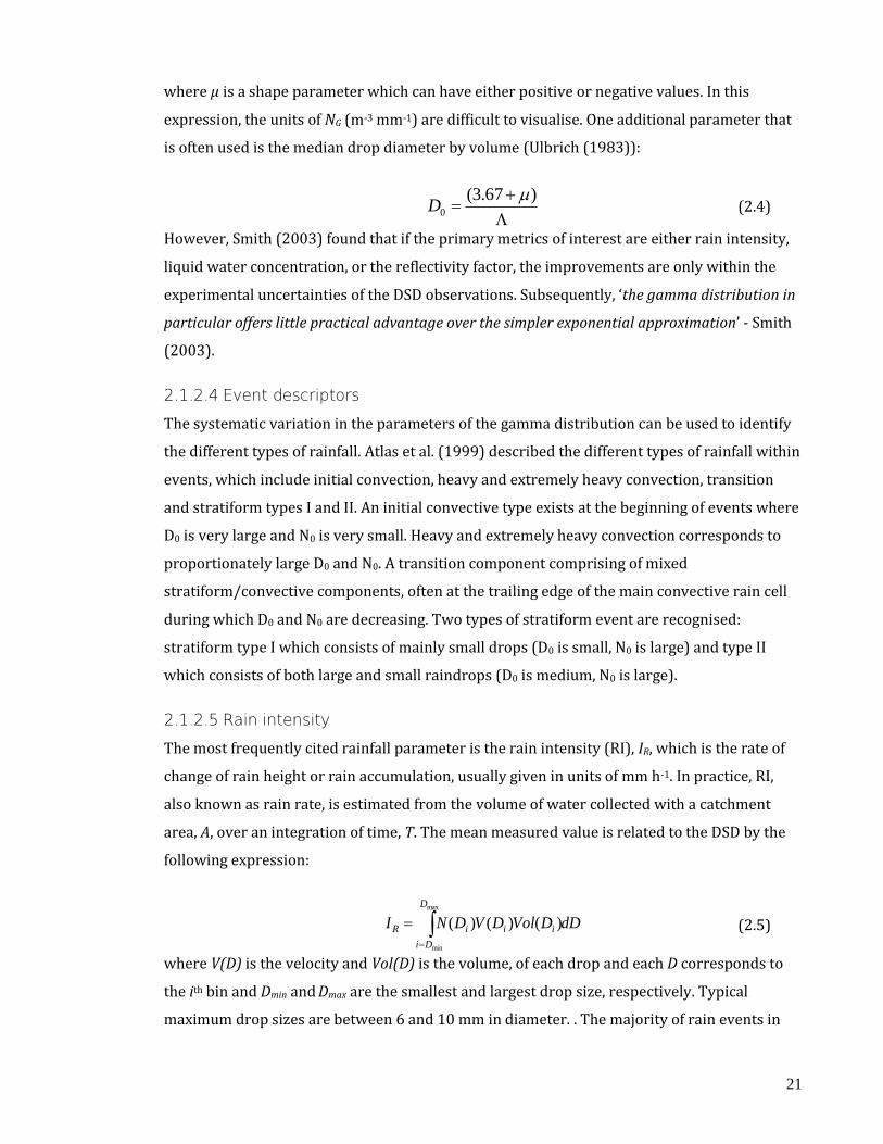
because of the ‘rather sharp physical change [that] occurs [in the terminal velocity] at d = 1.4

mm’. Note that their single equation for all drop sizes is adequate up to 7mm (see Figure 2.2).

The power law relations (Vt=aDb) of Liu and Orville (1969) and Atlas and Ulbrich (1977) are

mostly inaccurate due to neglecting drag. The logarithmic law of Best (1950) proposed Vt =

9.43 - 9.43 exp(-(D/1.77)1.147), which slightly underestimates between 2 and 5 mm (c.f. Figure

2.3). Atlas et al. (1973) suggested a similar exponential Vt = 9.65 – 10.3 exp(-0.65 D), which

fits better, but still underestimates between 3 and 4 mm.

24

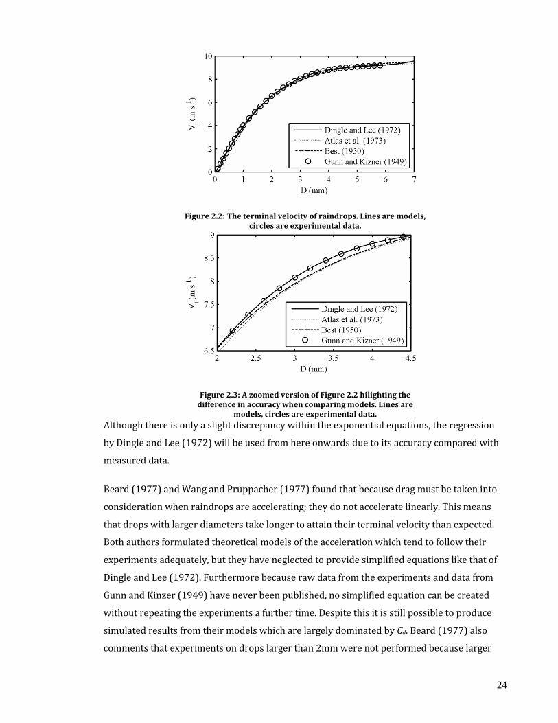
Figure 2.2: The terminal velocity of raindrops. Lines are models, circles are experimental data.

Figure 2.3: A zoomed version of Figure 2.2 hilighting the difference in accuracy when comparing models. Lines are

models, circles are experimental data.

Although there is only a slight discrepancy within the exponential equations, the regression

by Dingle and Lee (1972) will be used from here onwards due to its accuracy compared with

measured data.

Beard (1977) and Wang and Pruppacher (1977) found that because drag must be taken into

consideration when raindrops are accelerating; they do not accelerate linearly. This means

that drops with larger diameters take longer to attain their terminal velocity than expected.

Both authors formulated theoretical models of the acceleration which tend to follow their

experiments adequately, but they have neglected to provide simplified equations like that of

Dingle and Lee (1972). Furthermore because raw data from the experiments and data from

Gunn and Kinzer (1949) have never been published, no simplified equation can be created

without repeating the experiments a further time. Despite this it is still possible to produce

simulated results from their models which are largely dominated by Cd. Beard (1977) also

comments that experiments on drops larger than 2mm were not performed because larger

25

drops ‘distort earlier in their fall’ which in turn ‘leads to a reduction in acceleration for larger

drops and a reduction in the distance to reach terminal velocity’.

Not surprisingly, Montero-Martínez et al. (2009) found that it is possible to have ‘super-

terminal’ drops due to many different events, for example a small drop can, upon breakup of a

larger drop, retain the larger drops velocity for a period of time. Also, terminal velocities are

relative to the surrounding air. At altitude, air parcels can have significant vertical velocities in

both up- and down-drafts. This complicates the link between DSD and rainfall intensity. The

actual fall-speed is required in (2.5) and use of the terminal velocity can lead to considerable

errors in intensity estimates. This is a serious problem for meteorological radars which

estimate one or two parameters of the DSD but are insensitive to fall-speed. As the vertical

component of air movement approaches zero near the ground, catchment instruments, such

as rain gauges and disdrometers, provide better estimates of rain parameters affected by fall

speed.

2.2.2 Drop kinetic energy The kinetic energy (KE) of an object is the energy it possesses due to motion. It is defined as

the work required to accelerate a body of given mass from rest to its current velocity. An

object gains KE when it accelerates and maintains it until its speed changes. There are several

different forms of associated KE (rotational, vibrational, translational) and raindrops can

possess all three. However, as a matter of simplification we will only consider translational

KE, the energy due to motion from one location to another, since the others are assumed to be

negligible3. The translational KE is related to the objects mass, m, and velocity by:

2

2

1mVEK (2.6)

With regards to rainfall, the specific KE can be expressed in two different ways: volume-

specific and time specific (Kinnell (1981) and Rosewell (1986)).

With a similar definition as the rain intensity the rain KE can be expressed in terms of

raindrop KE per unit area per unit time, the KE flux density (or similarly, the KE intensity).

Assuming an atmosphere with a homogeneous DSD, the mean KE flux density (EK,t) is related

to the DSD by:

3 The rotational and vibrational movements of a particular raindrop is a highly complex and chaotic process and the modelling offers a significant challenge, to an extent that it has not been attempted.

26

dDDEDNATEMaxD

Di

iKitK

min

)()(, (2.7)

where A is the catchment area (m2), T is the integration time, N(D) is the DSD, and EK(D) is the

drop kinetic energy. The mass of a raindrop is:

DDDm 3

6

1)( (2.8)

where ρD is the density of the water in the falling drop, and D is the diameter of the equivalent

spherical drop. Therefore, equation (2.7) can be rewritten as:

MaxD

Di

iiiD

tK dDDVDDNATE

min

)()(12

23,

(2.9)

Volume-specific kinetic energy, EK,D, is often used by geomorphologists (Salles et al. (2002)

and has units of energy per unit area and per unit rain depth (J m-2 mm-1) and is derived from

the DSD by:

dDDDN

DVDDNAE

MaxD

Di ii

iiiDDK

min

3

23

,)(

)()(

2

(2.10)

From here on, the former definition of time-specific kinetic energy will be referred to as the

KE flux density.

The two expressions for the kinetic energy are linearly related, but more important is the link

between the rain intensity and the KE flux density. The subject has received considerable

attention, e.g. Salles et al. (2002) and Van Dijk et al. (2002). However, all studies are limited by

lack of data. Salles et al. (2002) note that ‘For the future... there is a need to provide more

detailed information on the DSD’. Even so, Van Dijk et al. (2002) produced equation (2.1) but

stated that when comparing the empirical model to real data a considerable average error of

10% was observed.

))042.0exp(52.01(3.28, RDK IE (2.11)

2.2.3 Sound generation When considering the choice of impacting material or substance, we require the lossless

conversion of impact energy into an electrical signal. One method of achieving this is to listen

to the sound that a raindrop makes upon impact. The advantages of using a solid would

include the manufacture and the maintenance of the instrument. However, we could not

guarantee that all of the drop’s energy would be converted into a sound. Furthermore, there is

significant literature on the physical modelling of a raindrop impact on a hard surface, but

27

little on the actual sound produced. The assumption follows that a wetted surface would

sound different to a dry one and differing impacting trajectories could have a significant

effects on the data. Furthermore, and more importantly, is that it would be more difficult to

position impacting drops due the increased speed of sound within the solid.

The most obvious solution is to allow the drop to land in a tank of water. This ensures that the

drop will hit a similar surface every time (neglecting the effects of surface waves). Many

experimental details regarding sound creation underwater have already been established

(Franz (1959), Pumphrey et al. (1989), Medwin et al. (1990), Manzello and Yang (2002),

Prosperetti and Oguz (1993)). They have shown that an impacting drop produces a number of

different signals transducer’s output. Further work has attempted to model this process, (Guo

and Williams (1991), Oguz and Prosperetti (1991)) and others have used this information to

create total sound profiles and measures of their respective event’s (see §2.4).

The impact of raindrops on the water’s surface generates a sharp initial pressure rise,

corresponding to radiated sound of short duration (between 10 and 40 μs) and a damped

pressure wave with predominantly low frequency content (below 600 Hz) associated with a

near-field hydrodynamic effect. Raindrops also cause strongly radiating air bubbles that are

formed from several tens to hundreds of milliseconds after the impact. These bubbles oscillate

and radiate sound with typical frequencies of 10-20 kHz for up to 10ms before reaching a

state of equilibrium. In laboratory studies using a 26 m long vertical utilities shaft and an

anechoic water tank (a 1.5 m high and 1.5 m diameter cylindrical redwood barrel with a lining

of redwood wedges), Medwin et al. (1992) have carried out a comprehensive analysis of the

acoustic signatures for drops of different sizes, and have found that the relative proportions of

impact and bubble noise vary with drop size. Drops below 0.7 mm in diameter were not

heard. Drops with diameters in the range 0.8 to 1.1 mm (associated with drizzle) cause an

impulse lasting for less than 10 μs and loud bubble noise across the frequency range 12 to 21

kHz. Typically, drops with diameters in the range 1.1 to 2.2 mm cause a loud impact noise but

do not create bubbles. Large drops with diameters above 2.2 mm cause very loud impact and

bubble noise across the frequency range 1 to 50 kHz, although not all large drops create

bubbles. Medwin et al. (1992) derived an empirical relationship between the peak frequency

of the bubble noise in the range 12 to 21 kHz and the raindrop volume. Several authors have

shown that the acoustic signature of the pressure wave associated with raindrop impact on a

water surface can be used for drop size measurement (Pumphrey et al. (1989), Mani and Pillai

(2004)).

28

Figure 2.4: A typical measured droplet impact and bubble signal using the AWTD.

Figure 2.4 illustrates an acoustic signal measured by a hydrophone, generated by the impact

of a raindrop on a water surface. The signal around 0.7 ms is the impact pulse while the

damped ringing from 2.3 ms onwards is due to bubble oscillation. For this illustration, the

time interval between impact and bubble noise has been reduced for clarity. Typical durations

are between 1 and 500 ms.

2.2.3.1 Entrainment

The damped sinusoid produced from trapped air provides the greatest problem in acoustic

disdrometry. Bubble signals have little relation to their impacting drop, do not occur on every

impact event, and are determined by three scenarios (Prosperetti and Oguz (1993)). Also,

when the bubble signal is produced, it is significantly larger in amplitude than any

corresponding impact signal. If another drop was to land at the same time as a bubble, this

could complicate the impact extraction process.

Regular entrainment (Franz (1959), Pumphrey et al. (1989)) is the name given to the process

where a bubble is created repeatedly when a droplet impacts on the surface of a liquid,

usually water. Several authors developed the mechanics of entrainment (see Prosperetti and

Oguz (1993)), and found that there are a number of scenarios when entrainment can occur.

Regular entrainment occurs when a crater is formed in the water after an impact. As the liquid

returns to its equilibrium, combined with the fact that the bottom part of the cavity still has

momentum, the sides of the crater can collapse or pinch-off due to a travelling capillary wave.

The resulting void at the bottom part of the crater forms a bubble.

Very large drops are affected by air resistance and tend to form an oblate shape that produces

an impact more like a water-hammer model. Upon large drop impacts the preceding air is

forced into the water which develops into an ‘azimuthal necklace’ of bubbles (Thoroddsen

29

et al. (2003)). This necklace then tends to form a number of stable bubbles due to their

surface tension.

The third type of entrainment is formed when after an initial large impact; further smaller

droplets are ejected from the impact site and create their own bubbles conforming to the first

two types of entrainment. This can be due to funnel formation and separation from a crater

collapse or from crown formation that is ejected into the air when a crater is formed with a

very large energy impact.

Irrespective of the type of entrainment, the resultant bubble will be subject to the

comparatively large pressure of being underwater. This will compress the bubble until a point

where its surface tension is greater than the force exerted on the bubble. The bubble will then

expand again oscillating until the two pressures reach equilibrium. Because the entrained air

is not spherical, there will also be spherical harmonic oscillations until it regains spherical

equilibrium.

2.2.3.2 Impact

Our interest in the pulse produced upon impact is justified by experimental results that show

that it is proportional to the impacting drop’s size and velocity (§ 2.2.3). Pumphrey et al.

(1989) reported that ‘the true initial impact pressure is proportional to the impact velocity to a

power between 2.5 and 3’. This result compounds the work of Franz (1959) who suggests that

the pressure is proportional to the velocity to a power of 3. Furthermore, the impact pressure

was also stated as proportional to the drop diameter to a power of 2.1 ±0.6, assuming a

terminal velocity.

Medwin et al. (1990) formalised the impact theory by taking results at different points within

a water tank and forcing impacts at increasing incidence angles. They found that impact sound

radiates as a one-sided dipole in the far field because the water’s surface acted as a reflector.

Furthermore, they also found that when a drop incidence is away from the normal, the impact

acoustic energy increases significantly. They supply an example that the pressure is increased

by 30% at an incidence angle of 20°. An interesting note is that a 20° incidence angle for a 1

mm drop at its terminal velocity corresponds to a wind speed of only 1.3 m s-1. The increase in

pressure is accounted by the decrease in probability of bubble entrainment; hence, some of

the energy that would have been used in creating a bubble has been transferred to the impact.

Several authors have formulated theoretical models of the impact process. Guo and Williams

(1991) based their model on an examination of the flow and the radiated compressive waves

30

due to the impact. They showed that ‘the impact causes rapid momentum exchange between

the falling fluid elements and those in the water body’. Their analysis verifies the analogy with a

water-hammer model. They also note the difficulty of trying to predict amplitudes after

reflection on the surface, but deny the necessity because it has ‘no effect on the energy carried

by the waves’. It does, however, affect the pressure waveform. Also, as a side note, their

equations show that the acoustic energy of an impact is proportional to the kinetic energy

carried by the drop. It is not clear whether this statement holds for impacts that create a

bubble.

Oguz and Prosperetti (1991) intended to prove that the variation in spectral peaks was due to

bubbles and not impacts (see §2.4), as it had previously been thought. They developed an

intuitive equation that describes the amount of pressure produced by an impact. The form of

the equation is correct, but the proportionality of the powers has been widely debated.

Pumphrey et al. (1989) specify that the pressure is proportional to the power of between 2.5

and 3 and proportional to the drop diameter raised to between 1.6 and 1.8. Other estimates

are that the impact pressure varies as VD2.8±0.2 and D1.5±0.2 (Pumphrey (1991)).

The variation in the influence of the velocity and diameter of a drop pertaining to an impact

pressure highlights the difficulty providing generalised models. The results of Pumphrey et al.

(1989) and Pumphrey (1991) neglect atmospheric conditions where drops are often

subjected to super- and sub-terminal velocities and various combinations of spherical

contortion and rotation. Hence, these experiments are unlikely to represent naturally

occurring rain and it is subsequently expected that the variation within these parameters

could alter dramatically.

Likhterov (1997) used the model of Guo and Williams (1991) to obtain a model of the

pressure field and use the Fourier transform to calculate the sound spectrum. It was shown

that the spectral density of the acoustic energy emitted by a falling sphere decreases by

approximately 4.3 dB per octave. This verifies the assumption that the impact signal can be

modelled as a non-ideal impulse.

2.3 An appraisal of current disdrometers In order to create a list of metrics to improve and compare against, it is necessary to

understand the principals of competing types of disdrometer.

31

2.3.1 Joss-Waldvogel The Joss-Waldvogel disdrometer (Joss and Waldvogel (1967)), also known as an impact

disdrometer, is an instrument that converts the force produced by individual raindrops into a

DSD.

Figure 2.5: The Joss-Waldvogel Impact disdrometer (courtesy of Distromet Ltd.)

The heart of the sensor is an electromechanical transducer, which in construction is similar to

a microphone and which has a catchment area of 50 cm2, or 0.005 m2. The instrument consists

of two parts: a cylindrical outer body that is fixed and a central column attached to a

membrane at the top. Two coils are located around the outside of the lower part of the

cylindrical shape of which a magnet in the central column is allowed to move freely in the

vertical axis. When a hydrometeor hits the membrane, it pushes the magnet through one of

the coils. This induces a resonant voltage into the coil which is then fed into a series of

amplifiers.

The current induced in the coil is proportional to the drop’s kinetic energy, but the lack of

rigidity within the system will cause the membrane to resonate after the impulse-like impact.

The authors compensate the resonance by driving the second coil to bring the system back to

equilibrium. They state that for drops of less than 3 mm this resonance is less than 1 ms and

for greater than 3 mm is a logarithmic function of the previous and subsequent drops (e.g. 4

mm then 1 mm = 14 ms); this is an example of dead-time. The impulse readings are then

collated into bins to form an arrival DSD.

After the device had become commercialised, Kinnell (1976) produced a paper that questions

the accuracy of the Joss-Waldvogel disdrometer. The author cited that inaccuracies were due

to ‘variations in factors such as raindrop velocity and raindrop shape generated by air

movements might produce unacceptable errors in the measurement of raindrop size by the [Joss-

Waldvogel] disdrometer’. Joss and Waldvogel (1977) provided a rebuttal to Kinnell’s

32

comments by calculating the standard deviation of the terminal velocity and shape of

raindrops. They found that Kinnel’s deviation of ‘more than 50%’ was unrealistic and used

data that showed that the deviation was ‘less than 4%’. The variation in drop shape was found

to be ‘about 2%’.

2.3.2 Thies Clima laser precipitation monitor The Thies Clima disdrometer is a modern laser precipitation monitor (LPM) using a parallel

780 nm infrared light-beam with a catchment area of approximately 45.6 cm2 (or 0.00456

m2). The manufacturers claim that the device can discriminate between all types of

precipitation: rain, hail, sleet and snow, by measuring both the size and the fall speed of the

hydrometeor. It measures the size by monitoring the scattering of the infrared light; the

amplitude corresponds to the size of the particle.

Figure 2.6: The Thies Clima Laser Precipitation Monitor (LPM) (courtesy of Thies Clima)

The velocity is calculated from the time it takes the particle to traverse the light beam. This

causes the LPM to underestimate the kinetic energy of a drop since it cannot measure the

horizontal velocity. Hence, although the AWTD may represent the KE flux density of an event

more accurately, after KE flux density data comparison with the LPM, high wind speed events

may appear to have a greater than normal variance.

The instrument can report information in a number of modes. A particle event transmission

reports the size and fall speed of a hydrometeor each time the beam is broken. It reports the

velocity and size of each particle along with a calculated oblate size if the particle’s velocity is

indicative of an oblate shape. After communication with Thies Clima engineers, the maximum

number of drops per second that the instrument can report is limited by the communication

speed. They did not provide quantification, so a simple simulation was created. By generating

a Marshall-Palmer DSD for different rainfall rates, we can integrate the product of N(D) and

V(D). This will yield the total number of drops falling through an area of 1 m2 per second. Each

33

LPM particle event message is 48 bytes4 long, where each byte is accompanied by a stop bit.

After normalising the drop data to the catchment of the LPM, a theoretical bit rate can be

estimated from a notional RI.

It can be seen from Figure 2.7 that

for a RI of 100 mm h-1 the bit rate

required is approximately 25 kb s-1.

Using a bit rate of 56.7 kb s-1 will

ensure that even in large storms, the

communication of arrival data will

still be possible. In practise, the peak

intensity before data corruption is

reduced due to the stochastic arrival

of drops. When each drop is detected

a data record is sent to the host

computer. If a second drop arrives during transmission of this data record, it is truncated and

the second record is transmitted. This can happen at any rain rate. However, for this project

the highest rain rate recorded was 42 mm h-1 where only 0.05% of drop records were

affected.

The disdrometer can also report in a DSD mode, which collates drop size and velocity

information over a number of user defined integration times, the smallest of which is 1

minute. In this text we prefer to use the particle event mode in its raw form as we can then

perform analyses on sub-minute integration times.

The accuracy of the LPM has been debated for some time. Although the error in the

measurement of the size of the hydrometeor is small, significant errors can arise over a longer

period of time. Lanzinger et al. (2006) found a problem with 2 out 3 LPM instruments on test

routinely reported a daily precipitation amount of 15 to 20% above that of the other, trusted

precipitation gauges on the site. Furthermore, Upton et al. (2007) and Brawn (2009) found

that depending on wind direction, the gauge would severely underestimate DSD populations

due to masking by the end of the instrument. Also the fall speeds, especially for smaller drops,

reported by different LPM’s vary appreciably from one disdrometer to another. Although,

these could have been caused by errors in experimental setup; for example if they were

compared in laboratory conditions, the difference is likely to be negligible.

4 One byte is 8 bits.

Figure 2.7: The required Thies Clima LPM bit rate for various rain intensities.

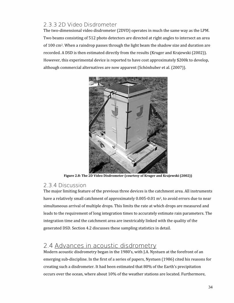
34

2.3.3 2D Video Disdrometer The two-dimensional video disdrometer (2DVD) operates in much the same way as the LPM.

Two beams consisting of 512 photo detectors are directed at right angles to intersect an area

of 100 cm2. When a raindrop passes through the light beam the shadow size and duration are

recorded. A DSD is then estimated directly from the results (Kruger and Krajewski (2002)).

However, this experimental device is reported to have cost approximately $200k to develop,

although commercial alternatives are now apparent (Schönhuber et al. (2007)).

Figure 2.8: The 2D Video Disdrometer (courtesy of Kruger and Krajewski (2002))

2.3.4 Discussion The major limiting feature of the previous three devices is the catchment area. All instruments

have a relatively small catchment of approximately 0.005-0.01 m2, to avoid errors due to near

simultaneous arrival of multiple drops. This limits the rate at which drops are measured and

leads to the requirement of long integration times to accurately estimate rain parameters. The

integration time and the catchment area are inextricably linked with the quality of the

generated DSD. Section 4.2 discusses these sampling statistics in detail.

2.4 Advances in acoustic disdrometry Modern acoustic disdrometry began in the 1980’s, with J.A. Nystuen at the forefront of an

emerging sub-discipline. In the first of a series of papers, Nystuen (1986) cited his reasons for

creating such a disdrometer. It had been estimated that 80% of the Earth’s precipitation

occurs over the ocean, where about 10% of the weather stations are located. Furthermore,

35

these weather stations are located mostly on islands, which are poorly distributed and where

orographic5 effects bias the measurements. Ship-board rain gauges are also often used, but

are affected by spray, instability and wind effects.

Ground and satellite-based meteorological radars are ubiquitous, but even now suffer from an

almost total lack of accurate surface measurements from oceanic environments, which are

required for calibration and verification. Nystuen proposed6 monitoring the ambient noise

generated by raindrops striking the surface during rainstorms. He created a system consisting

of a single hydrophone and electronics that could be deployed by a mooring, buoy or ship.

This setup would reduce the fair weather bias and provide a large spatial average, which was

dependant on the depth of the deployment. He then performed a frequency transformation

(FFT) to analyse the spectrum created by the rain. He found that rainfall can be detected even

in the presence of wind due to the spectral shape of the rain. He noted a high sensitivity at 15

kHz to the rainfall intensity, even for very low values (this was later attributed to entrainment

noise). He also created a simplified model of the impact process that was later improved by

other authors.

Nystuen and Farmer (1987) improved upon Nysten’s previous work by investigating the

effect of wind on the shape of the spectrum with mixed results. They found that the wind does

have a strong influence on the sound generated by two methods. The horizontal component of

the wind increases the net impact velocity and shifts the frequency of the peak and surface

waves spread the distribution of impact velocities causing the spectral peak to broaden.

Pumphrey et al. (1989) and Laville et al. (1991) later verified that the spectral peak around 15

kHz was due to the entrainment of bubbles. Pumphrey et al. (1989) proved this by adding a

surfactant to reduce the surface tension of the liquid so that entrainment would not occur; the

spectral peak disappeared. Laville et al. (1991) performed a short time Fourier transform

(also known as the Gabor transform) to look at the spectrum as events occur (i.e. impacts and

bubbles). Leighton et al. (1998) later used a similar method to detect the presence of bubbles

within a liquid.

2.4.1 Total acoustic intensity inversions Nystuen et al. (1993) first established a relationship between the acoustic intensity and the

rainfall intensity. They found that optimal correlation coefficients were obtained for

5 The physical geography of mountains and mountain ranges. 6 Previous authors in the 1950-60’s had recognised that much of the sound in oceans originated from rain events.

36

frequencies below 10 kHz (where their correlation coefficient was approximately 0.8) for

wind speeds of up to 15 m s-1. However, they state that the inaccuracy in the estimation occurs

from an overestimation during the beginning of a rain event and then an underestimation

later in the same event. They attribute this to changes in the DSD during the lifetime of the

event. For example, in convective events, large drops often represent a larger proportion of

the liquid volume at the beginning of the event than later in the same event. Further analysis

shows that the algorithm is more sensitive to larger drops; hence, it is more correctly an

estimate of the rainfall rate from large raindrops rather than total rainfall intensity.

Nystuen (1996) then introduced the concept of acoustical rainfall analysis (ARA) to use the

underwater sound generated by precipitation to detect, classify and quantify rainfall. The

author used laboratory experiments as a guide to devise an algorithm that would estimate the

DSD and other parameters from the acoustic intensity. Because of the sensitivity to larger

drops, the algorithm presents a very high correlation coefficient (0.93) for the similarly

sensitive, radar reflectivity.

Nystuen (2001) finally published the paper that revised and presented the previous work in a

single instrument and algorithm. He coined the term acoustic disdrometer as it could be

favourably compared to other disdrometers over thousands of minutes of results, including a

Joss-Waldvogel impact disdrometer (§2.3.1). The author found that the inversion between

acoustic intensity and rainfall intensity had a correlation coefficient of between 0.84 and 0.9,

depending on the disdrometer being compared, noting that this is higher than the algorithm

of Nystuen (1996). However, this algorithm uses conditional assumptions, based on the

acoustic intensity, to compensate for the overpowering sound of larger drops. Therefore, the

acoustic disdrometer’s inversion to form the DSD appears highly fragmented, yielding only 4,

or sometimes 2 (for low rain intensities) DSD parameters. This is clearly inadequate to

produce a description of arbitrary DSDs but may be sufficient to estimate the parameters of an

exponential or Gamma distribution.

Furthermore, although not investigated fully, Nystuen (2001) also realised that a high

resolution temporal analysis of rainfall is also possible. His analysis revealed subcells within

the convective rainfall with timescales of 2-5 minutes showing an extremely rapid onset and

cessation of rain at timescales shorter than can be measure by the majority of rain gauges. He

also identifies sub-minute variation within sub-cells that could be another indicator of rainfall

type.

37

Indeed, Nystuen and Amitai (2003) published a paper revealing 5 second resolution

(integration time) rainfall data, where they saw an event maximum of 1600 mm h-1. These

extreme values are not recorded by the other types of rain gauges because of the inherent

sampling limitations. Further work used the spectral and temporal characteristics as a way to

classify event types.

Ma et al. (2005) continued Nystuen’s work by refining the model that converted the acoustic

intensity into a rainfall intensity, based upon the logarithmic slope of the spectrum of the

acoustic intensity, which yields promising results. Using these models, the authors are able to

reconstruct the acoustic intensity spectrum from raw rain intensity data.

2.4.2 Direct inversion from impact pressures Another possibility of inversion is to form a DSD from individual impacts. This process uses

the measurements of individual impacts followed by individual inversion into a specific bin

within the DSD. This is a direct method in the sense it forms a DSD from individual events,

rather than integration of a longer event. By far, the most challenging task is to recognise that

an impact occurred within a significant amount of noise.

Mani and Pillai (2004) first investigated the problem of impact detection. They found that

bubbles contaminated the raw data and had to produce an algorithm that neglected the

bubbles. However, there are a number of areas that the authors have not discussed and the

results are questionable. Firstly, the authors state that a drop size is proportional to the

amplitude and the duration of the resonance of the water tank. Their own results show that at

a resonance of 64 Hz, they require a delay of 0.1 s for the decay to return to equilibrium, for a

fairly large drop. At this rate, they could only measure 10 drops a second, which is several

orders of magnitude lower than current disdrometers. Secondly, their detection algorithm

depends on differentiating the signal to yield a drop detection. The author’s data was sampled

at 48 ks s-1, which would (optimally) only yield a single data point at the moment of impact. If

a higher sampling rate was used, the author would have noticed that the impact is in fact not

impulse-like at all. Because of the low sampling rate, the equipment would likely miss many

drops, or at best produce an underestimate of the drop size. Thirdly, the authors produce a

graph that attempts to verify that the instrument readings confirm an adjacent tipping bucket

rain gauge. If these experiments were performed in a real event (of which 100 mm h-1 is

claimed – surely unfeasible according to the 0.1 s resonance period), then the majority of the

raindrops would be missed due to the high thresholding requirement at those rain intensities,

which would then yield an incorrect volume measurement. Finally, the authors also do not

38

state how they converted the resonance pressure into a drop size, aside from stating that it is

proportional.

2.5 Summary The field of meteorological instrumentation and acoustic disdrometry is clearly still an active

research area for scientists and engineers, many dedicating much of their academic lives to

the subject.

This chapter has reviewed several meteorological principles beginning with the hydrological

cycle (§2.1.1). The transport of water into the atmosphere was discussed along with the

associated formation and precipitation of hydrometeors. Section 2.1.2 established the concept

of a drop size distribution (DSD) which is one of the most cited descriptors of rain. Typically,

Marshall-Palmer (M-P) or gamma distributions are used to model an atmospheric DSD. The

rain intensity, approximately the fourth moment of the DSD, is another commonly used

measure of rainfall.

Section 2.2 considers the impact process upon a body of water. First, examples of the typical

velocities and kinetic energies are illustrated. The conversion of kinetic energy to sound is

then considered since an impacting drop interacts with the surface of the liquid in several

ways. At the initial moment of impact, a vicious impulse-like shockwave emanates spherically

from the impact site. The amplitude of the impact signal is dependent on the drop’s velocity

and size (analogous to the kinetic energy). In the moments that follow, a crater is formed and

subsequently can collapse. Whether the crater collapses or not is dependent on a number of

variables, including both the velocity and drop size.

An appraisal of current disdrometers was considered in section 2.3, establishing the various

advantages and disadvantages of other devices. The Thies Clima Laser Precipitation Monitor

will be used as a comparison for the AWTD.

Finally, research specific to acoustic disdrometry was analysed in section 2.4. Here, it was

established that several previous authors have attempted to use the underwater sound of rain

as a measure of the atmospheric rain intensity and DSD, with varying degrees of success.

39

Chapter 3: System design

A simple yet flexible prototype system is important to develop and test the AWTD concept. It

consists of several hardware components that fully optimise the performance of the AWTD.

This chapter deals with the design and manufacture of each sub-system.

Section 3.1 introduces the most basic part of the system, the water tank that will capture the

raindrops. Inside the tank are hydrophones that will listen to the drops which will then be

sampled by a data acquisition (DAQ) device. The hydrophone placement is optimised to

control errors due to drop physics and the DAQ.

Section 3.2 designs the electronics that converts the high impedance, low amplitude

hydrophone signal into a form that is more suitable for the DAQ. Impedance matching and

noise performance is important, so an in-depth analysis of both will be performed.

Section 3.3 investigates the errors that can arise from impact reflections. To mitigate, a

combination of anechoic linings are designed to absorb a significant amount of the incident

sound energy. The result is an absorber that is orders of magnitude cheaper than

commercially available anechoic linings with a similar performance.

40

Figure 3.1: The experimental acoustic water tank disdrometer. PC and electronics located elsewhere for

protection.

3.1 System components

3.1.1 Hydrophones Electro-acoustic transducers designed for underwater use have the same purpose as a

microphone or loudspeaker used in air: they are designed to efficiently convert acoustical to

electrical energy and vice versa. The desire for optimal power conversion prevents the

adoption of loudspeakers underwater or hydrophones in air. Loudspeakers and microphones

have been specifically designed to match the acoustical impedance of air. Since the acoustical

impedance of water is approximately 3500 times that of air, the mismatch would result in a

huge loss (Caruthers (1977)).

3.1.1.1 A comparison between underwater and air acoustics

Sound waves are propagating pressure and density fluctuations in a medium caused by

molecular motion. For small amplitudes the general wave equation can be expressed as:

01

2

2

2

2

t

p

cp (3.1)

41

where p is the dynamic pressure and c is the speed of sound. A simple description of the

sound field is the solution of (3.1) in one dimension (x) as a sinusoidal travelling wave:

ft

xptxp 2

2sin),( 0 (3.2)

where p0 is the amplitude of the wave, λ is the wavelength, f is the frequency and φ is the

phase shift. Equation (3.2) can also be expressed as:

tkxptxp sin),( 0 (3.3)

where k is the angular wave number (2π/λ) and ω is the angular frequency (2πf).

It is worthwhile to consider the differences in the parameters of the above equations for air

and water (Rosen et al. (1992)):

The speed of sound in water is approximately 4.4 times higher in water than it is in air.

Hence acoustic wavelengths are longer underwater than they are in air.

High frequencies in water are strongly attenuated. For most applications the useful

frequencies in water are generally below 40 kHz.

Absorption in water is much less than the absorption in air; 1 dB/km against 100

dB/km at 10 kHz, respectively (Kuttruff (2007))

For many applications, the intensity of an acoustic field is more useful than an absolute

measurement of pressure. The intensity, I, is a measure of power, P, per unit area, A,

perpendicular to the direction of propagation. Hence:

c

p

A

PI

2

2

(3.4)

where p is the root mean square (RMS) pressure, ρ is the density of medium and c is the speed

of sound within the medium.

The average power emitted by a source with respect to time, t (neglecting propagation delay),

is obtained by integrating the intensity over a surface completely enclosing the source:

dttItPA

)()( (3.5)

The power flowing through a sphere of radius, r, emitted by an isotropic source is a function

of the radial coordinate only. Hence:

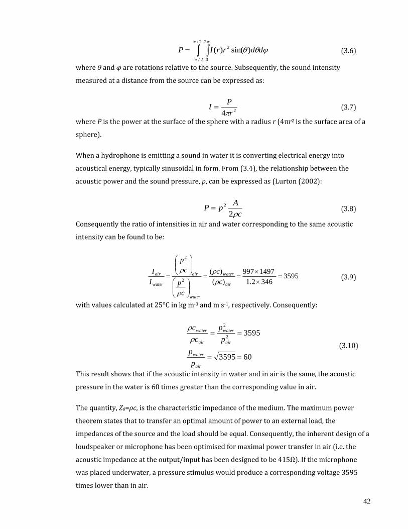
42

2/

2/

2

0

2 )sin()(

ddrrIP (3.6)

where θ and φ are rotations relative to the source. Subsequently, the sound intensity

measured at a distance from the source can be expressed as:

24 r

PI

(3.7)

where P is the power at the surface of the sphere with a radius r (4πr2 is the surface area of a

sphere).

When a hydrophone is emitting a sound in water it is converting electrical energy into

acoustical energy, typically sinusoidal in form. From (3.4), the relationship between the

acoustic power and the sound pressure, p, can be expressed as (Lurton (2002):

c

ApP

2

2 (3.8)

Consequently the ratio of intensities in air and water corresponding to the same acoustic

intensity can be found to be:

35953461.2

1497997

)(

)(2

2

air

water

water

air

water

air

c

c

c

p

c

p

I

I

(3.9)

with values calculated at 25°C in kg m-3 and m s-1, respectively. Consequently:

603595

35952

2

air

water

air

water

air

water

p

p

p

p

c

c

(3.10)

This result shows that if the acoustic intensity in water and in air is the same, the acoustic

pressure in the water is 60 times greater than the corresponding value in air.

The quantity, Z0=ρc, is the characteristic impedance of the medium. The maximum power

theorem states that to transfer an optimal amount of power to an external load, the

impedances of the source and the load should be equal. Consequently, the inherent design of a

loudspeaker or microphone has been optimised for maximal power transfer in air (i.e. the

acoustic impedance at the output/input has been designed to be 415Ω). If the microphone

was placed underwater, a pressure stimulus would produce a corresponding voltage 3595

times lower than in air.

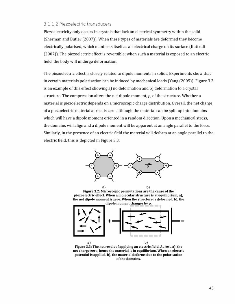
43

3.1.1.2 Piezoelectric transducers

Piezoelectricity only occurs in crystals that lack an electrical symmetry within the solid

(Sherman and Butler (2007)). When these types of materials are deformed they become

electrically polarised, which manifests itself as an electrical charge on its surface (Kuttruff

(2007)). The piezoelectric effect is reversible; when such a material is exposed to an electric

field, the body will undergo deformation.

The piezoelectric effect is closely related to dipole moments in solids. Experiments show that

in certain materials polarisation can be induced by mechanical loads (Yang (2005)). Figure 3.2

is an example of this effect showing a) no deformation and b) deformation to a crystal

structure. The compression alters the net dipole moment, p, of the structure. Whether a

material is piezoelectric depends on a microscopic charge distribution. Overall, the net charge

of a piezoelectric material at rest is zero although the material can be split up into domains

which will have a dipole moment oriented in a random direction. Upon a mechanical stress,

the domains will align and a dipole moment will be apparent at an angle parallel to the force.

Similarly, in the presence of an electric field the material will deform at an angle parallel to the

electric field; this is depicted in Figure 3.3.

Figure 3.2: Microscopic permutations are the cause of the

piezoelectric effect. When a molecular structure is at equilibrium, a), the net dipole moment is zero. When the structure is deformed, b), the

dipole moment changes by p.

Figure 3.3: The net result of applying an electric field. At rest, a), the

net charge zero, hence the material is in equilibrium. When an electric potential is applied, b), the material deforms due to the polarisation

of the domains.

44

3.1.1.3 External impedance mismatches

Power losses due to the characteristic impedance mismatch between the water and the

hydrophone are caused by reflections and refractions at a boundary layer. Consider an

interface between two media. According to the law of reflection, an incident wave with an

angle of incidence, θ, will reflect at the boundary with the same angle. Furthermore, some

proportion of the incident wave will enter the medium. This is known as the transmitted or

refracted wave, since typically it proceeds in a different direction characterised by the

refraction angle θ'. Both angles are related by:

)'sin(

'

)sin(

cc (3.11)

Here, c and c' are the speeds of sound in either medium; in optics, this is known as Snell’s law.

The ratio between the amplitudes of the transmitted and reflected waves can be shown to be:

'coscos'

'coscos'

00

00

ZZ

ZZR

(3.12)

and:

'coscos'

cos'2

00

0

ZZ

ZT

(3.13)

Equation (3.13) shows that the transmission depends on the angle of incidence. Also, if Z0=Z0',

then the entire wave is transmitted.

Therefore, to optimise power transmission, the piezoelectric element must be coated in a

protective outer layer that matches the acoustic impedance of water. Any incident sound

energy is transferred to the element with minimal loss. Furthermore, the element should be a

material that has a very high acoustic impedance. The sound energy is then reflected which

places the greatest amount of stress upon the crystal structure.

Hydrophone manufacturers typically mould bare piezoelectric materials in polyurethane

rubber due to its versatility. It also possesses an acoustic impedance that is very close to that

of water (Mott et al. (2002)). At 25°C and normal incidence, the transmission coefficient for a

polyurethane rubber is 0.95. A typical reflection coefficient at the polyurethane-piezoelectric

interface is 0.85 (Piezo Systems Inc. (2010)).

Electrical impedance matching is also important to maximise power conversion. This is

discussed in §3.2.

45

3.1.1.4 Hydrophone choice

Four Sonar Research and Development (SRD) Ltd. HS-150 hydrophones were chosen due to

their wide range and sensitivity. With a resonance at 150 kHz the hydrophone has a flat

working region from 100 Hz to 100 kHz (±3dB), omnidirectional to 280° (±1dB) and a

sensitivity of -204 dBV re. 1 μPa (-204 dB Volts relative to 1 micropascal). Although the

hydrophones are not officially calibrated, a calibration was performed by measuring the

received amplitude from a known distance. A multiplier is then applied in the software to

compensate for less sensitive hydrophones. Note that this also calibrates the amplifiers (see

§3.2.3.1).

3.1.2 Water tank dimensions A tank of water is required to provide a sustainable and consistent surface for raindrops to

impact upon. A cylindrical plastic (high density polyethylene – HDPE) tank with an outer

radius of 0.4 m, an inner radius of 0.35 m (after lining) and a depth of 0.59 m, was chosen

because of its local availability and its size. Ultimately, the size of the tank is limited by the

sensitivity of the hydrophones and the electronics. This sets a limit on the size of drop that can

be heard.

Furthermore, from §2.2.3.2, the amplitude of the sound created by an impact radiates as a one

sided dipole, directing sound energy downward in a cos(θ) pattern where θ is the angle

between a vector in the direction of the falling drop and the radiation direction. For example,

for a drop falling vertically, a hydrophone directly beneath the impact (i.e. at an angle of 0°)

will hear 100% of the impact energy). The power of the sound at a depth, h, below the surface

over a listening area, L, to be given by:

dLpaIP )(cos 20 (3.14)

where I0 is the sound intensity at the surface and a(p) describes the attenuation due to

spherical spreading and absorption along the path p. This has been verified by Medwin et al.

(1990). The absorption in water ranges up to 10 dB/km at 50 kHz. Since the path distances

within the tank are less than 1 metre, we can assume that there are negligible amounts of

absorption and only spherical losses are present. Since the amplitude of the sound is

proportional to the square root of the power, equation (3.14) can then be written as:

r

AP)cos(

(3.15)

where A is the received amplitude and r is the distance to the receiver. Equation (3.15) can

then be used to estimate the proportional amplitude received at a hydrophone. For example,

46

consider a hydrophone placed at a depth of h and at a perpendicular distance d away from the

impact (see Figure 3.4).

Figure 3.4: An image depicting the dipole effect on hydrophone placement.

The distance to the receiver, r, can be rewritten as h/cos(θ), yielding the amplitude to be

proportional to cos2(θ)/h. Therefore, at a depth (h) of 0.59 m, then we would receive 50% of

the amplitude at an angle of 57°, or at a distance, d, of 0.91 m.

This, along with a definition of the minimum discernable drop size (see §7.4.1), constrains the

tank to a certain depth and area. As an example, consider that we want to be able to discern

any drop of diameter greater than 2 mm. If our example system had a SNR of 2 at a depth of

0.59 m, for an impacting drop at terminal velocity, then a single hydrophone would not be

able to hear the drop if it was further than 0.91 m away from the hydrophone perpendicular

to the impacting drop’s vector. For simplicity, if we were only to use a single hydrophone, this

would yield a maximum tank radius of 0.91 m; any impacts beyond this radius would be

indistinguishable from noise.

This effect can be seen in Figure 3.5, which calculates the relative dipole loss when an impact

occurs at an extremity of the tank, on the opposite side of the hydrophone at a depth of 0.59

m. For example, if the impact is 0.35 m, from the centre of the tank the opposite hydrophone is

d+0.35 m away from the impact, where d is hydrophone offset from the centre of the tank.

(Note that the results in Figure 3.5 are using the previous assumption of an SNR of 2: if only

50% of the energy arrived at the hydrophone, the impact would be indistinguishable from

noise, hence, a 100% relative loss.)

47

Figure 3.5: The relative loss due to the dipole effect against an increasing hydrophone spacing.

3.1.3 Data acquisition The purpose of a data acquisition, (DAQ), card is to accurately convert an analogue signal into

a digital representation. Due to the sampling theorem a perfect conversion is impossible, but

realistic compromises can represent the signal with a certain degree of accuracy.

The DAQ card to be used in this project is located on a spare PCI slot within a standard

Windows XP PC. The type is a National Instruments PCI-4462 which has a maximum sampling

rate of 204 kS/s (thousands of samples per second) at a resolution of 24 bits. It also has four

inputs that can be simultaneously sampled and onboard anti-aliasing filters.

From here on, the data will be sampled at 200 kS/s, which yields one measurement every 5 μs.

Assuming that the peak of an impact pulse is an accurate representation of the impact time7

then the spatial resolution is:

mmmmf

cct 36.0735.0

200000

1450 (3.16)

where the speed of sound in water at 10 °C is approximately 1450 m s-1. The spatial resolution

is much smaller than the size of the smallest discernable raindrop (see §7.4.1).

The objective of the hydrophone array is to locate the original position of the impact. Because

the impact sound can only travel through the water at a finite speed, each hydrophone will

hear the impact at different times; this is known as the time of arrival, (TOA).

Consider 2 hydrophones with spacing ±d m away from the centre of the tank upon the same

axis in 2-dimensional space. If an impact occurred at the extremity of the tank, (i.e. the impact

7 Note that this may not be true. For example, the peak may occur in the middle of two samples causing a ‘chopped’ effect. The peak is also affected by the dipole dependence and noise.

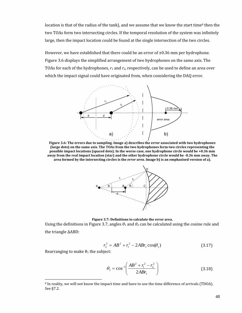
48

location is that of the radius of the tank), and we assume that we know the start time8 then the

two TOAs form two intersecting circles. If the temporal resolution of the system was infinitely

large, then the impact location could be found at the single intersection of the two circles.

However, we have established that there could be an error of ±0.36 mm per hydrophone.

Figure 3.6 displays the simplified arrangement of two hydrophones on the same axis. The

TOAs for each of the hydrophones, r1 and r2, respectively, can be used to define an area over

which the impact signal could have originated from, when considering the DAQ error.

Figure 3.6: The errors due to sampling. Image a) describes the error associated with two hydrophones (large dots) on the same axis. The TOAs from the two hydrophones form two circles representing the possible impact locations (spaced dots). In the worse case, one hydrophone circle would be +0.36 mm

away from the real impact location (star) and the other hydrophone circle would be -0.36 mm away. The area formed by the intersecting circles is the error area. Image b) is an emphasised version of a).

Figure 3.7: Definitions to calculate the error area.

Using the definitions in Figure 3.7, angles θ1 and θ2 can be calculated using the cosine rule and

the triangle ΔABD:

)cos(2 11

2

1

22

2 ABrrABr (3.17)

Rearranging to make θ1 the subject:

1

2

2

2

1

21

12

cosABr

rrAB (3.18)

8 In reality, we will not know the impact time and have to use the time difference of arrivals (TDOA). See §7.2.

49

Note that the length CD is equal for both triangles ΔADC and ΔBDC, hence:

2

111

2

2211

)cos(cos

)cos()cos(

r

r

rr

(3.19)

Using the two angles and the radii of the circles we can calculate the areas of the arcs.

However, we only require the outside area of the smaller arc. Hence, calculating the area

outside of triangles ΔADC and ΔBDC:

)01.0(

)sin()cos(2

1

2

12)(

2

)sin()cos(2

1

2

12)(

2

12

22222

2222

11112

1111

area

AAA

rrrBDCareaarcA

rrrADCareaarcA

err

(3.20)

Figure 3.8: The sampling error with respect to hydrophone placement. 100% error is determined at the

point where the hydrophones are touching (±1 cm).

Figure 3.8 plots the sampling error, Aerr, for several hydrophone spacing’s for an impact at an

extremity (±0.35 m - the size of the experimental tank). An error of 100% is defined as the

point where the two hydrophones would be touching (±1 cm). This is referred to as area(0.01)

in equation (3.20). It can be seen that the loss is approximately linear down to ±0.1 m. Below

0.1 m, the error becomes exponential which continues to a point where the two TOA circles

cease to intersect, which implies that the impact could have occurred anywhere around the

extremity of the tank.

The error is minimised at a point where one hydrophone is directly underneath the impact

and the other is located at the opposite side. However, if the opposite hydrophone is too far

away, it may not be able to discern the impact (like in §3.1.2). A combination of these two

errors must be considered.

50

3.1.4 Optimal hydrophone placement The combination of the dipole effect, §3.1.2, and the sampling errors, §3.1.3, (i.e. the average

of two percentage errors) will yield an optimum hydrophone spacing where the two errors

are minimised. This calculation can be seen in Figure 3.9 which provides a spacing of

approximately ±10 cm from the centre of the tank. Note that this assumes that the two errors

are equal in measure and equally important.

Figure 3.9: The combination of the dipole and sampling errors to yield a minimum error which occurs at

approximately ±0.1 m from the centre of the tank.

3.2 Electronics Unamplified hydrophone sensitivities are approximately -200 decibel volts relative to 1

micropascal (dBV re. 1 μPa). A large raindrop impact generates pressures in the order of 1

Pascal at a depth of 0.5 m (Pumphrey (1991)), and so would produce a voltage change of 100

μV at the output. The output impedance of hydrophones is extremely high; only a matched

amplifier would be able to efficiently convert the pressure induced voltage into a useable

signal. In order to obtain a high dynamic range and perform an impedance transformation,

amplification is necessary. This section details the design of a pre-amplifier for the AWTD.

3.2.1 Overview Similar to §3.1.1.3, the electrical impedance of the acquisitioning system requires matching to

ensure conversion efficiency. However, making the impedance of the acquisitioning system

greater than the hydrophone can actually improve performance. Since ideally, a hydrophone

is a voltage controlled device only, hence (assuming infinite DC impedance), voltage efficiency

is important, unlike the optimised power efficiency of §3.1.1.3.

51

Figure 3.10: A component level model of a hydrophone. Bottom: internal, top: external.

Consider the mechanical properties of a piezoelectric material, a component level model of a

hydrophone can be created (c.f Figure 3.10). The top image models the external

characteristics of the hydrophone with RC and CC as the cable resistances and capacitances,

respectively. The lower part of the image models the inside of the hydrophone. RO and CO are

the output impedance of the hydrophone, where the resistive part, RO, is often above 108 Ω at

DC. Output capacitances, CO, often range between 1 and 10 nF. The final section of the internal

hydrophone model, Vp, Cp and Lp, models the piezo element’s mechanical properties. Like a

mass on a spring analogy, the element will have a corresponding resonance, inertia and

momentum.

The resonance of the piezo element occurs

at fR Hz, which is a function of Cp, Lp and the

internal resistance of Vp. Just below fR and

where the AC-coupling effect of Cp causes

the sensitivity to tend to zero, is ideally flat.

It is in within this range that hydrophones

are used. A stylised frequency-sensitivity

plot for a hydrophone can be seen in Figure

3.11.

3.2.2 Requirements From previous discussions, it has become clear that an intermediate stage is required to

convert a high impedance input to a low impedance output so that the DAQ can accurately

sample the signal. Such impedance converters often also provide amplification as it adds very

little to the cost of the circuit. Hence, we require a:

high input impedance

Figure 3.11: A stylised frequency response of a

hydrophone.

52

low output impedance

small amount of gain, and

low noise

3.2.3 Design Interfacing the outputs of highly capacitive transducers such as hydrophones presents many

design challenges. Previously, designers had to use costly hybrid amplifiers consisting of

discrete low-noise JFETs in front of conventional operational amplifiers to achieve the high

input impedance and low levels of voltage and current noise required by these applications.

Today, modern designers can take advantage fully monolithic solutions that typically take the

form of JFET-input CMOS operational amplifiers. This not only meets the high impedance

requirement, but also provides a low noise, stable and simple platform.

From an exhaustive appraisal of current off-the-shelf high input impedance operational

amplifiers, the Analog Devices’ AD8066 operational amplifier provides the best compromise

between input impedance, voltage noise and current noise.

3.2.3.1 Charge Amplifier

Figure 3.12 depicts a charge amplifier configuration of

an operational amplifier. Charge amplifiers are

typically used to obtain large time constants (i.e.

response to low frequencies) whereas other types of

amplifiers struggle to cope with the long decay times

and tend to leak charge through biasing resistors. To

eliminate this, the charge amplifier uses a capacitor as

the negative feedback element, Cf, and as a result the

amplifier immediately transfers the charge at the

amplifier input to the feedback capacitor.

Since the voltage at the input is maintained at zero due to the properties of the operational

amplifier, the leakage charge generated by the transducer with respect to ground is greatly

reduced; hence the DC impedance is greatly increased. Using Ohm’s law the DC input

impedance will be the voltage divided by the current. Since the capacitor is attempting to keep

the input at zero volts (by matching the input voltage to the output voltage) the net current

flow is zero (ideally – there will be a finite lag time). As the current tends to zero, the input

impedance tends to infinity; this process is known as bootstrapping. Real operational

amplifiers are limited by their output voltage error (i.e. offset voltage × gain) and slew rate.

Figure 3.12: An operational amplifier in a

charge amplifier configuration.

53

The gain of the feedback amplifier is inversely proportional to the size of the feedback

capacitor and is independent of the transducer/cable capacitance. This is because the charge

generated by the transducer is directly transferred to the feedback capacitor, much like a

hydraulic system. Hence, the capacitance of the transducer cable does not influence the

magnitude of the output signal, unlike a voltage amplifier configuration. Therefore, the gain of

the amplifier can be found to be:

f

H

C

Cgain 1 (3.21)

Resistor, Rf, provides the input with a DC path to ground, which would otherwise cause the

output to float between the power rails. RB and CB are required to match the operational

amplifier’s input bias currents which should be set to the combination of the hydrophone and

feedback impedances. This allows a near zero potential difference between the inputs which

yields an offset output error close to zero. This further ensures a high input impedance due to

the bootstrapping.

3.2.3.2 Power Supply Filtering

Critical to any amplifier is its power supply. If a power supply contains any significant amount

of AC noise, it will be coupled into the operational amplifier and amplified at the output. One

method to ensure a clean supply is by filtering the DC voltage with passive inductors and

capacitors. Other more complicated adaptive analogue and digital methods do exist.

A series of 3 banks of 1 mH inductors and 1 mF capacitors form a low-pass tuned circuit

which have a cut-off frequency at 160 Hz with a roll-off of 60 dBV per decade. Note that the

equivalent series resistance (ESR) of the capacitors provide enough damping to prevent

unstable oscillation. This filter ensures that a negligible amount of power supply noise is

present above 1 kHz.

3.2.3.3 Schematic

Figure 3.13 is a full schematic of the pre-amplifier.

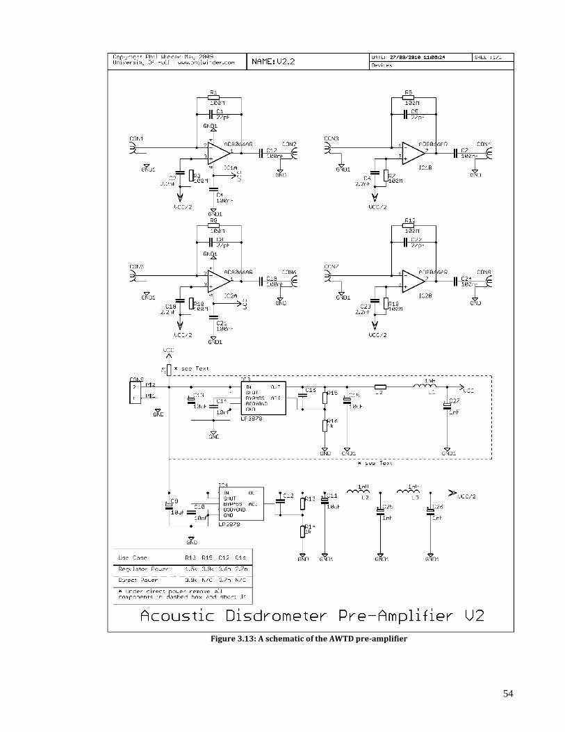
54

Figure 3.13: A schematic of the AWTD pre-amplifier

55

3.2.4 Noise A noise specification of the pre-amplifier is helpful in predicting signal to noise ratios (SNR)

and hence estimate the smallest discernable drop. Ultimately, the high input impedance

requirements of the amplifier will prevent the design of a very low noise amplifier. However, a

full noise analysis is important to understand where the main electronic noise sources

originate.

3.2.4.1 Voltage noise

From Figure 3.12, we can replace all the noise

generating components with Thevenin equivalent

voltage noise sources; this can be seen in Figure 3.14.

Since all the noise sources are independent, we can use

the principle of superposition to sum all of the

contributing errors.

3.2.4.1.1 Resistor noise Johnson noise is caused by the thermal agitation of

charge carriers in a conductor (also known as thermal

noise). This noise is present in all passive resistive

elements and has a uniform power spectral density. The noise power spectral density within a

resistor, R, is calculated by:

kTRe 4 (3.22) where e has units (V2/Hz), k is Boltzman’s constant and T the absolute temperature.

Furthermore, capacitors Cf and CB form a single pole low pass filter. At frequencies higher than

the cut-off frequency, fc=1/2πRC, the thermal noise will decrease due to increasing amounts of

current flow through the capacitor instead of the resistor. As f→∞, the current flowing

through either R tends to zero and hence does not add to the noise.

3.2.4.1.2 Hydrophone noise The internal noise of a hydrophone, eH, is caused by its energy dissipation mechanisms (i.e. the

electrical and mechanical dissipation factors of the transduction material and components,

Sherman and Butler (2007). Electrical and mechanical resistance allow internal thermal

energy to be lost and hence thermal energy within the hydrophone materials cause electrical

noise. It follows from the equivalent circuit concept that both the electrical and mechanical

losses can be represented by a Thevenin equivalent electrical series resistance, RH. Like other

resistors, the equivalent Johnson thermal noise voltage is then given by equation (3.22).

Figure 3.14: Charge amplifier noise

analysis.

56

At frequencies below resonance the mechanical resistances are small compared to the

mechanical reactance. Electrical dissipation follows the frequency dependence of the

mechanical reactance and is often the main loss mechanism and therefore the main internal

noise mechanism. In this case, it is possible to find the equivalent electrical resistance as a

function of the hydrophone’s capacitance, a material dependent loss factor and the frequency

(see Sherman and Butler (2007)).

Unfortunately, the material specifications or an equivalent noise figure were not available.

However, as an example, Sherman and Butler (2007) use a 2cm radius PZT-4 based

hydrophone and found that it has a theoretical thermal noise of 8dBV re. 1 μPa2 at 1 kHz.

3.2.4.1.3 Operational amplifier noise Although a component level analysis of the entire operational amplifier is possible, it is often

easiest to use quoted noise figures from a manufacturer’s datasheet. These values are

experimental and provide a more realistic value than one that is theoretically based, although

manufacturers are notorious for providing exaggerated parameters. For the AD8066, the

voltage noise is quoted as 7 nV/√Hz.

The input current noise, ia, also contributes to the voltage noise when it passes through a

resistor. The current noise for the AD8066 is 0.6 fA/√Hz.

3.2.4.1.4 Total voltage noise The total voltage noise can be calculated by the addition of all the contributing noise sources.

Each noise must be taken as the output power spectral density, since a number of sources are

affected by the circuit gain, A, (see §3.2.3.1). Hence, the output power spectral density of each

noise source, E, is:

fH

fH

aBa

f

Ha

fH

fH

aBaaA

f

HHHH

f

HBRBRB

fRfRf

RR

RRiRi

C

Ce

RR

RRiRiAeE

C

CkTRAeE

C

CkTRAeE

kTReE

1

14

14

4

(3.23)

Hence, the total noise power spectral density, ET, is:

57

fRR

RRiRiAeAkTRAkTRkTRE

fEEEEE

fH

fH

aBaaHBfT

AHRBRfT

2

222

2222

444 (3.24)

where f is the bandwidth. If the total voltage noise spectrum is assumed to be flat (i.e. filter

roll-off is above working frequencies and 1/f noise is now lower than the thermal noise (1/f

noise usually intersects the thermal noise at about 1 kHz) then to convert the power spectral

density into a voltage we can multiply by a frequency range and take the square-root.

Using the example hydrophone noise figure given in §3.2.4.1.2 and placing all other

resistances and operational amplifier noise figures into equation (3.24), it is possible to

calculate the amount of noise at the output of the pre-amplifier. Using a frequency range of 49

kHz (1-50 kHz) and a temperature of 283.15 K (10 °C) with the component values given in the

schematic (c.f. Figure 3.13) a theoretical minimum total noise of 163 μV RMS (equivalent to

2.5 mPa) can be expected. It is interesting to note that the majority of the noise originates

from the operational amplifier.

Furthermore, this does not take any external noise sources into consideration. For example,

mains noise will typically be the largest noise source.

3.2.5 Noise verification Figure 3.15 shows a randomly selected second of raw pre-amplifier output data. The RMS

value of this dataset (neglecting large peaks due to impacts and bubbles) is 720 μV indicating

that an extra 557 μV RMS of voltage noise is entering the system. This will decrease the signal

to noise ratio and ultimately reduce the sensitivity of the AWTD (i.e. increase the smallest

discernable drop size). The extra noise could be from a number of sources. The most likely

sources are the:

power supply

DAQ

hydrophones

PC, or

mains

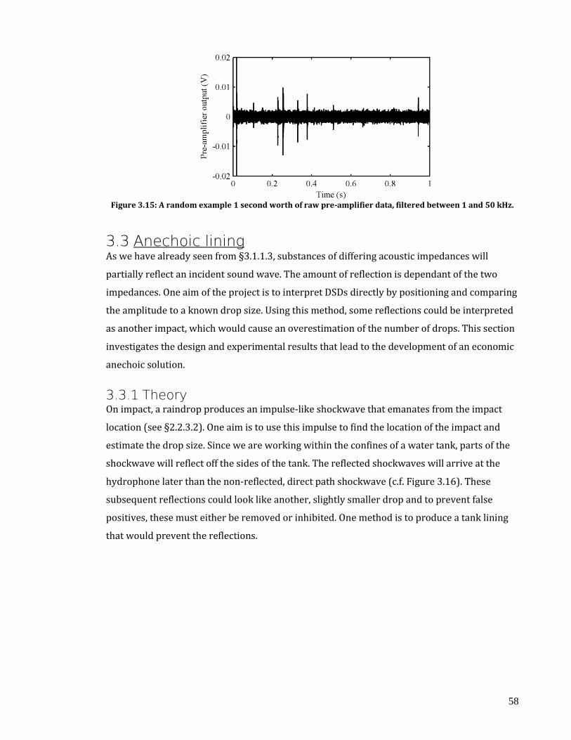
58

Figure 3.15: A random example 1 second worth of raw pre-amplifier data, filtered between 1 and 50 kHz.

3.3 Anechoic lining As we have already seen from §3.1.1.3, substances of differing acoustic impedances will

partially reflect an incident sound wave. The amount of reflection is dependant of the two

impedances. One aim of the project is to interpret DSDs directly by positioning and comparing

the amplitude to a known drop size. Using this method, some reflections could be interpreted

as another impact, which would cause an overestimation of the number of drops. This section

investigates the design and experimental results that lead to the development of an economic

anechoic solution.

3.3.1 Theory On impact, a raindrop produces an impulse-like shockwave that emanates from the impact

location (see §2.2.3.2). One aim is to use this impulse to find the location of the impact and

estimate the drop size. Since we are working within the confines of a water tank, parts of the

shockwave will reflect off the sides of the tank. The reflected shockwaves will arrive at the

hydrophone later than the non-reflected, direct path shockwave (c.f. Figure 3.16). These

subsequent reflections could look like another, slightly smaller drop and to prevent false

positives, these must either be removed or inhibited. One method is to produce a tank lining

that would prevent the reflections.

59

Figure 3.16: Charge amplifier noise analysis.

There are two possible solutions to this problem:

a. transmit all of the incident sound energy to outside the tank

b. absorb the sound energy within the lining.

Consider option a); the idea is to create a tank lining that would transmit all of the incident

sound energy to the air. First, we would have to design a lining that matches the impedance

between the water and the tank (high-density polyethylene Z≈2.3×106, water Z≈1.5×106) then

another lining on the outside to transmit the sound from the tank to the air (air Z≈412);

clearly the largest reflection will be between the tank-air interface.

This could be possible using a structure that gradually alters the acoustic impedance from that

of the tank to the air. A conical, or pyramidal based structure is often used, but this may cause

unforeseen refraction patterns and the entire tank would become cumbersome and fragile.

This also assumes a perfect contact between the impedance matching material and the tank,

which, over time, would be hard to guarantee; air pockets will form underneath the lining and

create another tank-air-lining interface.

For a better solution, b), rather than attempting to move the sound energy to another location,

we should try to absorb and dissipate internally. Typically there are three methods of sound

absorption:

1. resonant

2. porous

3. elastic

By creating a cavity in front of a good reflector, the space will become resonant at a particular

frequency. Any incident sound will set the material into vibration, particularly so near its

60

resonant frequency. Hence, work is performed setting the material into vibration and energy

is lost. Additional losses are also seen when the material transmits some of that energy into

the reflector through its mountings.

Porous materials contain many macro and microscopic holes and ducts. Porous losses supply

attenuation through viscosity and heat conduction effects along these ducts. Furthermore,

fibrous materials move in the presence of a pressure wave and the resultant internal inter-

fibre friction absorbs some of the energy.

Finally, elastic materials such as rubber absorb sound due to the frictional losses when the

material stretches or contracts. Molecules within the rubber collide and produce a frictional

loss.

All of these methods rely on the change in one form of energy to another. Methods 2 and 3

convert the sound energy into heat via friction and method 1 converts it into a kinetic energy

via the pressure of the sound wave.

So far, we have stressed the quantitative features of reflection and absorption of sound waves

at boundaries of various sorts. Now we consider what constitutes a good absorber of plane

waves. Maximum absorption can only occur if all of the sound energy actually enters the

material and hence, is not reflected. The solution is to find a material that is not only highly

absorptive, but also matches the acoustic impedance of water. If it does not, then the previous

impedance matching methods could be applied.

Furthermore, for a discussion of cost, it is necessary to compare commercial alternatives. A

tile of absorptive material 0.6×0.6 m is available from Precision Acoustics Ltd. located in

Dorchester. Unfortunately their products are mainly aimed at MHz frequencies; however, it

performed well in preliminary tests. Their datasheet specifies a transmission loss of between

0 and 14 dB between 0 and 50 kHz. The cost per slab is approximately £600, leading to a cost

of thousands to line the entire tank.

3.3.2 Results Reiterating §3.1.1.3, when a sound wave in a medium of acoustic impedance Z0 arrives at

some other medium of acoustic impedance Z1, part of the wave will be transmitted and the

rest reflected. The transmission, T, and reflection, R, coefficients can be found to be:

1011

1001

coscos

coscos

ZZ

ZZ

p

pR

i

r

(3.25)

61

and:

101

00

coscos

cos2

ZZ

Z

p

pT

i

t

(3.26)

where pi, pr and pt are the incident, reflected and transmitted acoustic pressures, respectively.

After some of the wave is transmitted into the second medium, some of the sound will reflect

on the next interface and reflect back to the original medium. Again, there will be another

transmission and some secondary reflected sound will penetrate back into the initial medium.

This continues until the amplitude of the sound within the second medium is zero. The total

acoustic pressure field can be described by the summation of the two waves, one travelling

forward and one backward. The total pressure field at the rear of the slab can be expressed as

one emerging wave. With these considerations, the total transmission coefficient, T, can be

described as (Davis (1934):

l

Z

Z

Z

Z

l

T2

cot4

2cot44

2

0

1

1

0

2

(3.27)

where l is the slab thickness and λ is the wavelength of the incident wave. Note that when a

slab thickness of π/2 (with respect to the wavelength, in radians) is used (or any integer

multiple of), all of the incident energy will be transmitted (i.e. T is a maximum). When an odd

multiple of π/4 is used, the transmission will be at a minimum. However, if the material

characteristic impedances Z0 and Z1 are correctly matched, there will be little difference

between the maximum and minimum transmission coefficients.

Figure 3.17: Transmission coefficient for a 1cm slab of: a) rubber, and b) aluminium, in water.

Figure 3.17 shows the transmission coefficient with two different materials against frequency.

When comparing the characteristic impedance of water, which is 1.48×106, to the impedance

62

of rubber, 1.47×106, and of aluminium, 17.3×106, it is clear to see why the rubber's

transmission coefficient is high (measurements in Ns/m3 - Honda (2009)).

Once the sound wave has entered the rubber, it will begin to distort and vibrate. Rubber is a

highly elastic material and the amount of absorption is dependent on the damping that the

vibration is subjected to. Through a number of viscoelastic processes that convert sound

energy into heat, the amount of absorption is termed the loss factor, η. This is ‘a measure of

the proportion of energy that is necessary to feed into the vibrating system in order to maintain

its vibrations with a constant amplitude’ - Ouis (2005).

Ouis (2005) developed a model to estimate the loss factor for rubber based upon the

material's parameters. The result, when using the parameters specified by the author, result

in Figure 3.18:

Figure 3.18: Predicted loss factor using the parameters from Ouis (2005).

The loss factor would then be inserted into a typical exponential describing harmonic motion

yielding a decaying sinusoid.

Because a drop impact creates a dipole-like sound field at the water's surface, the majority of

the energy will be travelling vertically downwards. Therefore, the majority of the reflections

will occur between the bottom of the tank and the water surface. Unfortunately it is not

possible to mitigate reflections on the water's surface, so the damping will only be half as

effective. This will reduce the loss factor by half. Furthermore, Ouis (2005) did not specify the

thickness of the rubber slab that he used and there is no relevant parametric data for the

natural rubber used in this test.

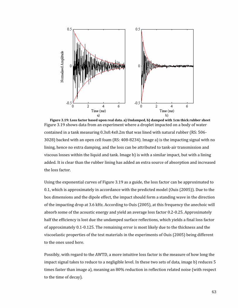
63

Figure 3.19: Loss factor based upon real data. a) Undamped, b) damped with 1cm thick rubber sheet

Figure 3.19 shows data from an experiment where a droplet impacted on a body of water

contained in a tank measuring 0.3x0.4x0.2m that was lined with natural rubber (RS: 506-

3028) backed with an open cell foam (RS: 408-8234). Image a) is the impacting signal with no

lining, hence no extra damping, and the loss can be attributed to tank-air transmission and

viscous losses within the liquid and tank. Image b) is with a similar impact, but with a lining

added. It is clear than the rubber lining has added an extra source of absorption and increased

the loss factor.

Using the exponential curves of Figure 3.19 as a guide, the loss factor can be approximated to

0.1, which is approximately in accordance with the predicted model (Ouis (2005)). Due to the

box dimensions and the dipole effect, the impact should form a standing wave in the direction

of the impacting drop at 3.6 kHz. According to Ouis (2005), at this frequency the anechoic will

absorb some of the acoustic energy and yield an average loss factor 0.2-0.25. Approximately

half the efficiency is lost due the undamped surface reflections, which yields a final loss factor

of approximately 0.1-0.125. The remaining error is most likely due to the thickness and the

viscoelastic properties of the test materials in the experiments of Ouis (2005) being different

to the ones used here.

Possibly, with regard to the AWTD, a more intuitive loss factor is the measure of how long the

impact signal takes to reduce to a negligible level. In these two sets of data, image b) reduces 5

times faster than image a), meaning an 80% reduction in reflection related noise (with respect

to the time of decay).

64

Furthermore, a 25mm thick open cell foam was added to provide a resonant cavity at about

50 kHz and create further porous losses, however the impedance match is expected to be

slightly worse than that of the rubber (No material parameters available).

3.3.3 Conclusions Using an anechoic lining will help later in the project by damping potential reflections off the

sides of the tank. This solution is at least 2 orders of magnitude cheaper than any commercial

alternative. The possibility of confusion between true impacts and reflections of impacts could

limit the accuracy of the system. By ensuring that the majority of the impacts received are

direct, the positioning algorithms in later chapters (see §7.2) will subsequently produce less

errors.

3.4 Summary The design of the tank that will be used to capture data has been considered. A full schematic

of the AWTD hardware can be seen in Figure 3.20.

Figure 3.20: Full AWTD hardware schematic

First, a description of the basic components within the system has been provided, which

comprised of: hydrophones to convert the sound energy into an electrical signal, a tank to

provide a catchment for the rain, a DAQ unit to convert the electrical signal into a digital one

and finally considered where the hydrophones will be placed. It was found that the amplitude

of the impact signal depended on the hydrophone placement, which was due to the dipole and

sampling errors.

Next, the electronics that provided an impedance match to that of the hydrophone were

designed. It was found that using an operational amplified in a charge amplifier configuration

is best suited to the task. The electronics poses a significant amount of noise within the

system and theoretical analysis has been considered, although experiments proved that the

65

background noise was larger than expected. This could be due to several external,

uncontrollable noise sources.

Finally, an investigation of anechoic linings was performed, and natural rubber was found to

be best absorber of sound energy due to its near identical acoustic impedance. The cost of this

is orders of magnitude lower than commercial alternatives. Using an anechoic will reduce the

errors cause by reflected impact pulses being used in the direct interpretation methods

(Chapter 7).

66

Chapter 4: Total sound field interpretation

This chapter describes the development of the total sound field method for the acoustic water

tank disdrometer (AWTD). The measurement of total sound field in a water tank removes the

majority of noise contamination sources present in marine measurements. This chapter

examines the measurement of rain intensity, kinetic energy and DSD from the total sound

field.

Section 4.1 describes the locality of the AWTD and details regarding the experiment. Section

4.2 investigates statistical problems arising from a small catchment area and develops

algorithms for estimating rain parameters from tank measurements. Section 4.3 compares

tank-derived parameters from those derived from measurements of a co-sited LPM. Section

4.4 discusses the use of total sound field measurements to generate a DSD.

4.1 Comparison of instrument measurements A Thies Clima Laser Precipitation Monitor (LPM) is sited within 0.5 m of the tank edge and at

the same level as the water’s surface. Both instruments are installed in a suburban garden in

Hull, UK [53.76735,-0.366345]. The instruments are approximately 10 m from the southern

aspect of a two-storey house and there are trees over 20 m tall approximately 50 m from the

67

instruments. Although the situation is far from ideal for accurate rain parameter

measurements, due to disturbance of the wind field by the buildings and trees, we are

interested in comparing parameters estimated from the LPM and the acoustic measurements

made in the tank. It is reasonable to expect the two instruments to experience the same rain

parameters.

The LPM is operated in event mode where the diameter and fall-speed of each drop is

recorded. This allows DSD and related parameters to be calculated with a range of integration

periods. A large amount of data is produced and this will begin to saturate the serial data

connection at rain intensities in excess of 100 mm h-1. However, rain at this intensity typically

occurs for only one or two minutes a year in Hull.

Over a period of eight months beginning in October 2009, rain events were observed with

simultaneous recording of the sound field in the water tank at the four hydrophones and the

drops arriving at the LPM. The objective was to determine what rain parameters, at what

temporal resolution, could be derived from the acoustic measurements. Both instruments

yield measurements affected by a range of systematic and random errors. When comparing

measurements it is important to understand what differences are significant. The largest

uncertainty is introduced by the relatively small sample volume of the LPM i.e. the drops

recorded by the LPM are unlikely to be representative of the DSD in the atmosphere above the

instruments. In the paragraphs below expressions for the uncertainty in measured rain

parameters in terms of the instrument sample volumes are derived.

4.2 Sampling statistics Rain measurements typically derive rain parameters from the raindrops in a sample volume

of atmosphere e.g. meteorological radar; or the raindrops that cross a horizontal catchment

area in an interval of time e.g. a rain gauge or disdrometer. The raindrops in the sample will

have different sizes and relative positions each time a measurement is performed, even if the

notional rain parameter e.g. rain intensity or rain kinetic energy, is constant. This yields a

temporal fluctuation in the measured parameter around the notional value and a distribution

of measured values, characterized by a variance.

The numbers and relative positions of raindrops in the atmosphere are determined by very

complex processes including coalescence and break-up, along with evaporation and turbulent

inertial sorting. Although this leads to some clustering, drop arrivals at a catchment are often

modelled as a Poisson process. The distribution of drops over some small diameter range i.e.

68

[D, D+dD], can be modelled as Poisson as drops of a particular size are likely to have been

produced by different, and uncorrelated, break-up events. The same arguments hold for the

arrival of raindrops at an instrument catchment area. This has been experimentally verified

by Joss and Waldvogel (1969). If we assume that the arrival of drops in a small size interval is

a Poisson process, (Onof et al. (2000)), this allows the calculation of the variation in rain

parameters derived from DSD measurements over a range of integration intervals. The

Poisson distribution is discrete and has the property that the mean is equal to the variance.

4.2.1 Sample errors in catchment rain measurements Instruments such as rain gauges and disdrometers measure rain parameters from the

raindrops that cross a catchment area A in an integration time T. These instruments can be

thought of as sampling a prism of atmosphere above the instrument with cross-section A and

height V(D)T, where V(D) is the fall-speed of drops of diameter D. The sample volume is larger

for larger raindrops with more rapid fall-speed. This is an advantage for disdrometers as a

higher proportion of large drops are measured, compared to a volume sampling instrument,

yielding better sampling statistics at the large diameter tail of the DSD. If a horizontal wind is

present, the sample prisms are no longer perpendicular to A, but have the same volume.

Consider a notional rain event with a uniform mean rain intensity of R mm h-1. If the sizes of

raindrops are Marshall-Palmer distributed, (Marshall and Palmer (1948)), then the mean

number of drops per unit volume, in the diameter interval [D, D+dD], is given by

dDeN(D)dD=Λ D0

, where Λ0 is a constant and R is a function of the mean rain intensity.

The mean number of drops in each size range, measured by the disdrometer is:

dDDNDdD=AT VD Ndisd (4.1)

where Ndisd(D) is the observed DSD. Due to the Poisson assumption, the variance of this

measurement is:

dDDNDdD=AT VD=NdDDNVar disddisd (4.2)

An estimate of N(D)dD derived from the disdrometer measurement is:

DATV

dDDN±

DATV

dDD NdDDN disd (4.3)

It is clear that diameter ranges with small numbers of measured drops yield poor estimates of

the number density of these drops in the atmosphere e.g. a bin with 10 measured drops yields

an atmospheric number density with a 30% relative error.

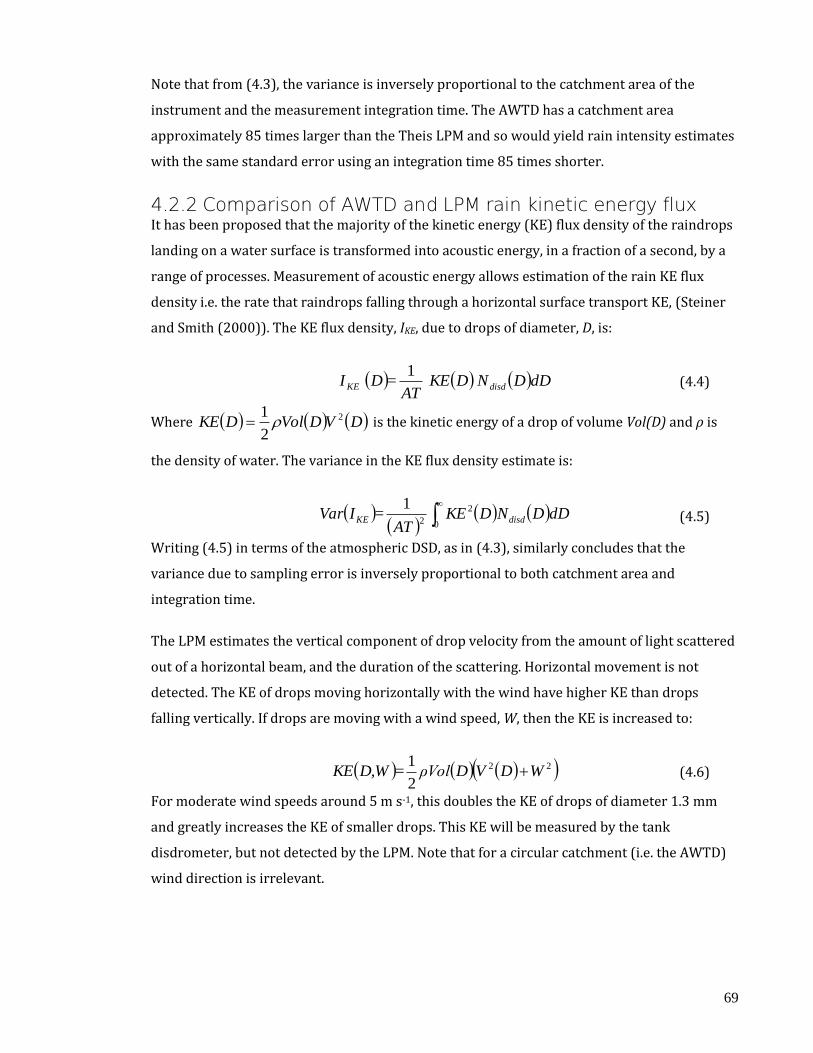
69

Note that from (4.3), the variance is inversely proportional to the catchment area of the

instrument and the measurement integration time. The AWTD has a catchment area

approximately 85 times larger than the Theis LPM and so would yield rain intensity estimates

with the same standard error using an integration time 85 times shorter.

4.2.2 Comparison of AWTD and LPM rain kinetic energy flux It has been proposed that the majority of the kinetic energy (KE) flux density of the raindrops

landing on a water surface is transformed into acoustic energy, in a fraction of a second, by a

range of processes. Measurement of acoustic energy allows estimation of the rain KE flux

density i.e. the rate that raindrops falling through a horizontal surface transport KE, (Steiner

and Smith (2000)). The KE flux density, IKE, due to drops of diameter, D, is:

dDD ND KEAT

=D I disdKE

1 (4.4)

Where DVDVolDKE 2

2

1 is the kinetic energy of a drop of volume Vol(D) and ρ is

the density of water. The variance in the KE flux density estimate is:

0

2

2

1dDDNDKE

AT=IVar disdKE (4.5)

Writing (4.5) in terms of the atmospheric DSD, as in (4.3), similarly concludes that the

variance due to sampling error is inversely proportional to both catchment area and

integration time.

The LPM estimates the vertical component of drop velocity from the amount of light scattered

out of a horizontal beam, and the duration of the scattering. Horizontal movement is not

detected. The KE of drops moving horizontally with the wind have higher KE than drops

falling vertically. If drops are moving with a wind speed, W, then the KE is increased to:

22

2

1WDVDρVol=D,WKE (4.6)

For moderate wind speeds around 5 m s-1, this doubles the KE of drops of diameter 1.3 mm

and greatly increases the KE of smaller drops. This KE will be measured by the tank

disdrometer, but not detected by the LPM. Note that for a circular catchment (i.e. the AWTD)

wind direction is irrelevant.

70

4.3 Establishing relationships

4.3.1 Rain kinetic energy flux The impact pulse and entrained bubble noise, due to the primary impact and splash products,

carry the bulk of the energy while much smaller amounts generate surface waves,

atmospheric sound and splash products that fall outside the tank. It is reasonable to assume

that the acoustic energy measured in the tank over a second or longer would be approximate

the kinetic energy carried by the raindrops falling onto the water surface. This hypothesis was

tested by comparing one minute, raindrop kinetic energy accumulations estimated using the

velocities and drop sizes measured by the LPM, with the total acoustic energy measured by an

average of the 4 tank hydrophones. Figure 4.1 is the scatter plot of these two quantities with

error bars indicating the standard deviations of LPM derived rain kinetic energy flux density

calculated using (4.5) and (4.6). All rain events over the eight months observation period

were used except for those the LPM determined were hail, snow or sleet. A total of 25 hours of

rain was observed with a maximum rain rate of 43 mm h-1. This is typical for the experiment

location.

Figure 4.1: Comparison of LPM derived raindrop kinetic energy flux density with total acoustic energy

integrated over one minute. The error bars indicate uncertainty due to sampling errors. Both the KE flux density and the total acoustic pressure are normalised to a catchment of 1 m2 over an integration time of 1

hour.

The measured acoustic energy needs to be adjusted at low rain intensities to remove the noise

inherent in the measurement electronics. As the system noise and rain generated signal are

uncorrelated, the total measured acoustic energy is the sum of noise plus signal energies. Data

at the noise floor have been removed.

71

The kinetic energy of falling drops needs to be corrected for horizontal movement with the

wind. Even for low wind speeds of several meters per second, a large proportion of raindrops

would be moving horizontally faster than they are falling. Therefore, the kinetic energy

derived from LPM measurements is expected to be an under-estimate. This under-estimation

will be more significant at lower rain rates where more drop kinetic energy is due to

horizontal movement. For this reason the points corresponding to low energy flux densities

deviate further from the regression line than due to sampling errors alone.

A linear fit of the scatter plot, (c.f. Figure 4.1), is plausible. Using least squares regression (LAR

method) the following parameters were found to fit KE to the total acoustic intensity, AI:

AIKE 3106.77 (4.7)

A Pearson correlation coefficient of 0.92 was found when using the parameters as illustrated

in Figure 4.1. This compares well to the correlation coefficients of Nystuen (2001), who found

coefficients between 0.79 and 0.94 for various combinations of disdrometers.

4.3.2 Rain intensity A similar process can be performed for rain intensity, (RI), estimated using the LPM. Generally

power-law relationships are used to link RI with KE, e.g. Salles et al. (2002). As KE has been

shown to be proportional to AI, a power-law relationship is expected between RI and AI.

Salles et al. (2002) suggest where 1.06≤β≤1.35. The exponent depends upon the

assumed form of DSD. This suggests a power-law relationship . RI is not affected

by the horizontal movement of raindrops although the kinetic energy is increased. Therefore,

more spread is expected when comparing RI to AI. Figure 4.2 is a scatter plot of RI against AI.

The LAR best fit of the log parameters indicate a power-law exponent of 0.68, which

considering the effect of the wind, is consistent with the results of Salles et al. (2002).

68.031060 AIRI (4.8)

The log parameters have a Pearson correlation coefficient of 0.81. This is lower than the

coefficient for KE, due to uncertainties introduced by wind and DSD variations, but still

reasonable for rain measurements. However the RI should still be viewed as a derived rather

than measured parameter.

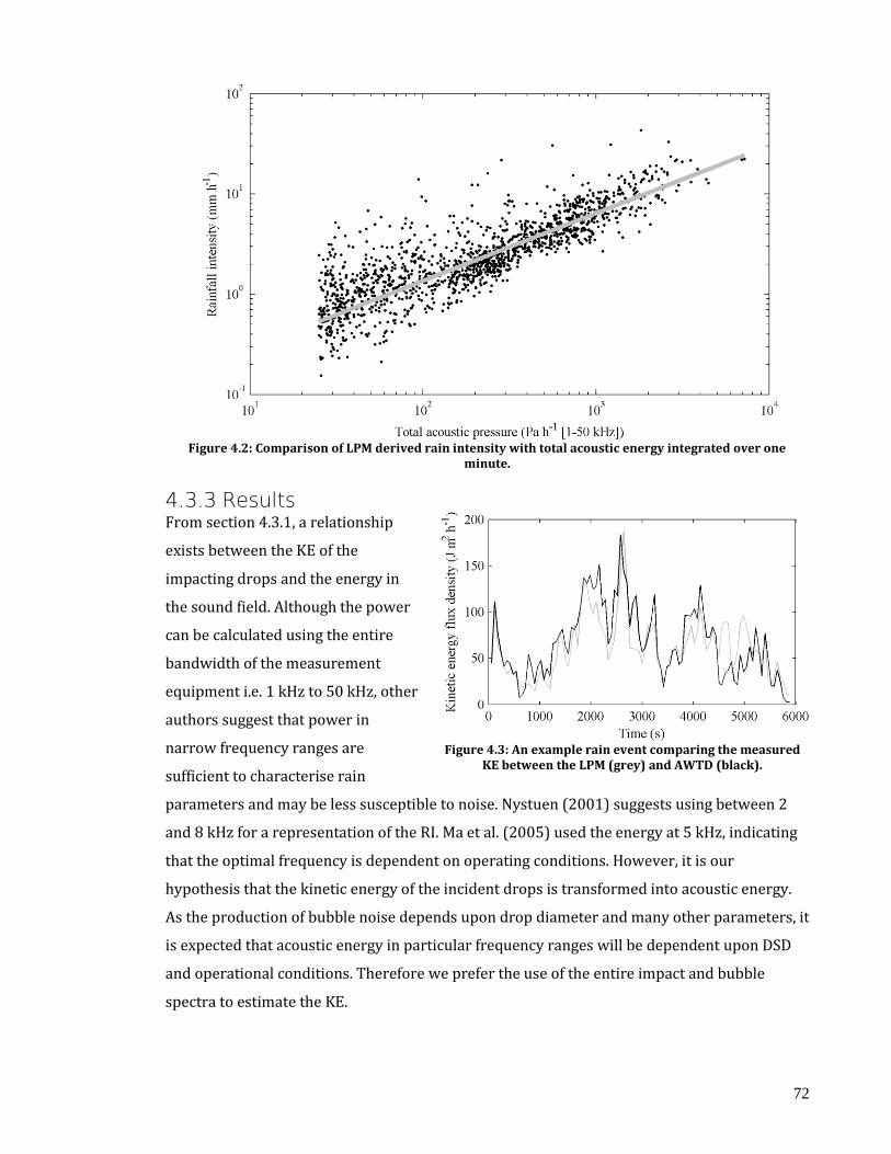
72

Figure 4.2: Comparison of LPM derived rain intensity with total acoustic energy integrated over one

minute.

4.3.3 Results From section 4.3.1, a relationship

exists between the KE of the

impacting drops and the energy in

the sound field. Although the power

can be calculated using the entire

bandwidth of the measurement

equipment i.e. 1 kHz to 50 kHz, other

authors suggest that power in

narrow frequency ranges are

sufficient to characterise rain

parameters and may be less susceptible to noise. Nystuen (2001) suggests using between 2

and 8 kHz for a representation of the RI. Ma et al. (2005) used the energy at 5 kHz, indicating

that the optimal frequency is dependent on operating conditions. However, it is our

hypothesis that the kinetic energy of the incident drops is transformed into acoustic energy.

As the production of bubble noise depends upon drop diameter and many other parameters, it

is expected that acoustic energy in particular frequency ranges will be dependent upon DSD

and operational conditions. Therefore we prefer the use of the entire impact and bubble

spectra to estimate the KE.

Figure 4.3: An example rain event comparing the measured

KE between the LPM (grey) and AWTD (black).

73

Figure 4.3 and Figure 4.4 illustrate

KE and RI time-series for a typical

rain event with RIs between 5 and 13

mm h-1, (c.f. Figure 4.4), calculated

using a one minute integration time.

For both graphs KE and RI are

measured using the LPM and

estimated using the AWTD and

empirical relations (4.7) and (4.8).

These show broad agreement with

differences due to the separation of catchment areas (approximately 0.5 m between

instruments) and volume sampling uncertainties. Nystuen (2001) measures the relative

performance of different disdrometers by the means of a Pearson correlation coefficient. The

coefficients range from 0.79 to 0.94 indicating that both the KE and RI conversions perform at

least as well as other commercial disdrometers.

4.3.4 Increasing the temporal resolution Section 4.2 established that the AWTD could provide rain parameters with an integration time

as short as one-second, with the same sampling errors as the LPM with a one-minute

integration time, due to its much larger catchment area. Figures 4.5 to 4.8 illustrate KE and RI

time-series for the same event. The AWTD data has been used to estimate these parameters

with an integration time of 10 and 1 s, and these have been compared with the one-minute

integration time LPM results.

Figure 4.4: An example rain event comparing the measured RI

between the LPM (grey) and AWTD (black).

74

Figure 4.5: Kinetic energy flux density time series derived from AWTD data, (grey) with a 10 second integration time compared to LPM data (black) with a 60 second integration time.

Figure 4.6: Rain intensity time series derived from AWTD data, (grey) with a 10 second integration time compared to LPM data (black) with a 60 second integration time.

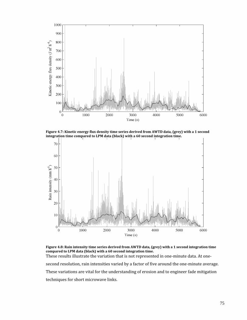
75

Figure 4.7: Kinetic energy flux density time series derived from AWTD data, (grey) with a 1 second integration time compared to LPM data (black) with a 60 second integration time.

Figure 4.8: Rain intensity time series derived from AWTD data, (grey) with a 1 second integration time compared to LPM data (black) with a 60 second integration time.

These results illustrate the variation that is not represented in one-minute data. At one-

second resolution, rain intensities varied by a factor of five around the one-minute average.

These variations are vital for the understanding of erosion and to engineer fade mitigation

techniques for short microwave links.

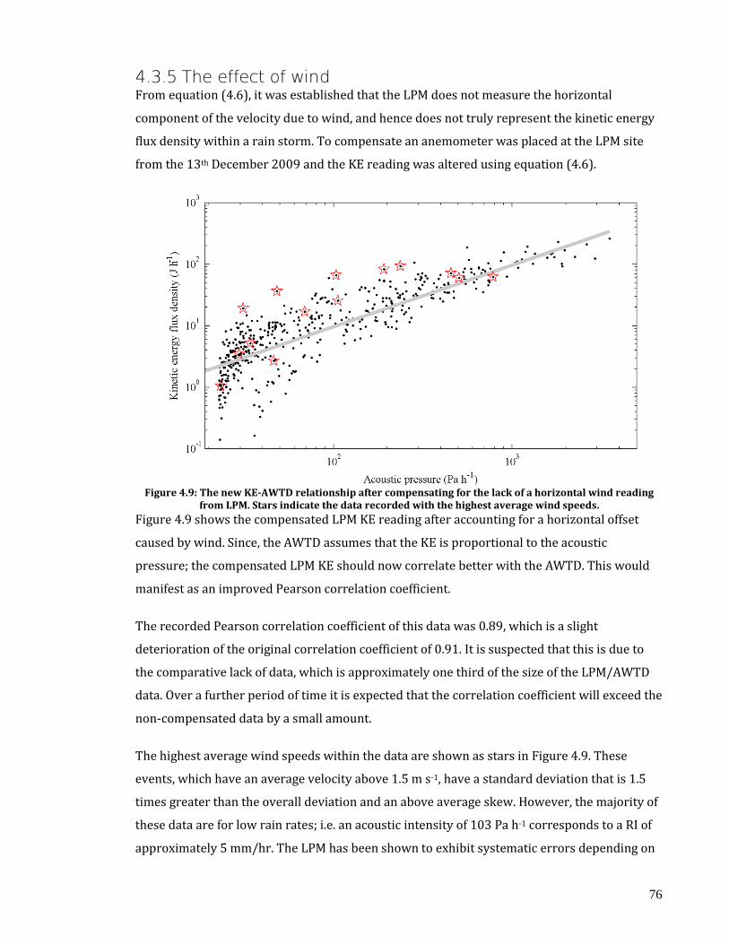
76

4.3.5 The effect of wind From equation (4.6), it was established that the LPM does not measure the horizontal

component of the velocity due to wind, and hence does not truly represent the kinetic energy

flux density within a rain storm. To compensate an anemometer was placed at the LPM site

from the 13th December 2009 and the KE reading was altered using equation (4.6).

Figure 4.9: The new KE-AWTD relationship after compensating for the lack of a horizontal wind reading

from LPM. Stars indicate the data recorded with the highest average wind speeds.

Figure 4.9 shows the compensated LPM KE reading after accounting for a horizontal offset

caused by wind. Since, the AWTD assumes that the KE is proportional to the acoustic

pressure; the compensated LPM KE should now correlate better with the AWTD. This would

manifest as an improved Pearson correlation coefficient.

The recorded Pearson correlation coefficient of this data was 0.89, which is a slight

deterioration of the original correlation coefficient of 0.91. It is suspected that this is due to

the comparative lack of data, which is approximately one third of the size of the LPM/AWTD

data. Over a further period of time it is expected that the correlation coefficient will exceed the

non-compensated data by a small amount.

The highest average wind speeds within the data are shown as stars in Figure 4.9. These

events, which have an average velocity above 1.5 m s-1, have a standard deviation that is 1.5

times greater than the overall deviation and an above average skew. However, the majority of

these data are for low rain rates; i.e. an acoustic intensity of 103 Pa h-1 corresponds to a RI of

approximately 5 mm/hr. The LPM has been shown to exhibit systematic errors depending on

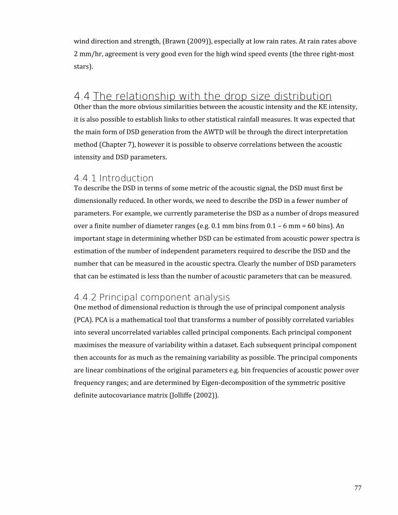
77

wind direction and strength, (Brawn (2009)), especially at low rain rates. At rain rates above

2 mm/hr, agreement is very good even for the high wind speed events (the three right-most

stars).

4.4 The relationship with the drop size distribution Other than the more obvious similarities between the acoustic intensity and the KE intensity,

it is also possible to establish links to other statistical rainfall measures. It was expected that

the main form of DSD generation from the AWTD will be through the direct interpretation

method (Chapter 7), however it is possible to observe correlations between the acoustic

intensity and DSD parameters.

4.4.1 Introduction To describe the DSD in terms of some metric of the acoustic signal, the DSD must first be

dimensionally reduced. In other words, we need to describe the DSD in a fewer number of

parameters. For example, we currently parameterise the DSD as a number of drops measured

over a finite number of diameter ranges (e.g. 0.1 mm bins from 0.1 – 6 mm = 60 bins). An

important stage in determining whether DSD can be estimated from acoustic power spectra is

estimation of the number of independent parameters required to describe the DSD and the

number that can be measured in the acoustic spectra. Clearly the number of DSD parameters

that can be estimated is less than the number of acoustic parameters that can be measured.

4.4.2 Principal component analysis One method of dimensional reduction is through the use of principal component analysis

(PCA). PCA is a mathematical tool that transforms a number of possibly correlated variables

into several uncorrelated variables called principal components. Each principal component

maximises the measure of variability within a dataset. Each subsequent principal component

then accounts for as much as the remaining variability as possible. The principal components

are linear combinations of the original parameters e.g. bin frequencies of acoustic power over

frequency ranges; and are determined by Eigen-decomposition of the symmetric positive

definite autocovariance matrix (Jolliffe (2002)).

78

Often the first few principal components, account

for most of the variability within the data, and

the later components are determined by noise.

Using 25 hours of rain data and DSD estimated

using the LPM with a one minute integration

time, the autocovariance matrix of the 60 bin

frequencies was calculated. Figure 4.10

illustrates a typical measured DSD (black) and

this is compared with the projection of this

distribution on the manifold spanned by the first

three principal components (grey). The important features of DSD were adequately described

using only the weights of the first three principal components. The standard Gamma DSD

distribution similarly has three parameters but would not be able to describe the features

evident in the measured DSD. Using a dataset containing a greater variety of event would

certainly lead to more important components and hence require more parameters.

The same analysis was applied to measured acoustic power spectra, calculated by numerical

FFT of 60 second intervals of measured total sound fields. Power spectra were averaged

across all four hydrophones. PCA yielded 3 principal components that accounted for 95% of

the variance. Regression analysis was then performed looking for linear relationships

between the 3 acoustic power spectra principal components and the 3 DSD components. No

statistically significant correlations were found.

Bubble noise is strongly localised in the 10 to 20 kHz range and is predominantly produced by

drops in the middle size range, unlike impact sound which is broad spectrum and produced by

all drops. This would seem to suggest it likely that the shape of the acoustic spectrum would

provide information on the DSD shape. However, this experiment has shown that the shape of

the acoustic spectrum is strongly influenced by other factors, such as wind, which changes the

way drops produce entrained bubbles.

4.4.3 Fitting distributions From section 2.1.2, when DSDs are averaged over a long period they can be described by a

variety of standard size distributions. The most cited is the Marshall-Palmer (MP) distribution

(Marshall and Palmer (1948) which is based on an exponential distribution. However, it was

later found that the DSD is more accurately described by a gamma distribution, (Ulbrich

Figure 4.10: An example DSD reconstruction

from three principal components.

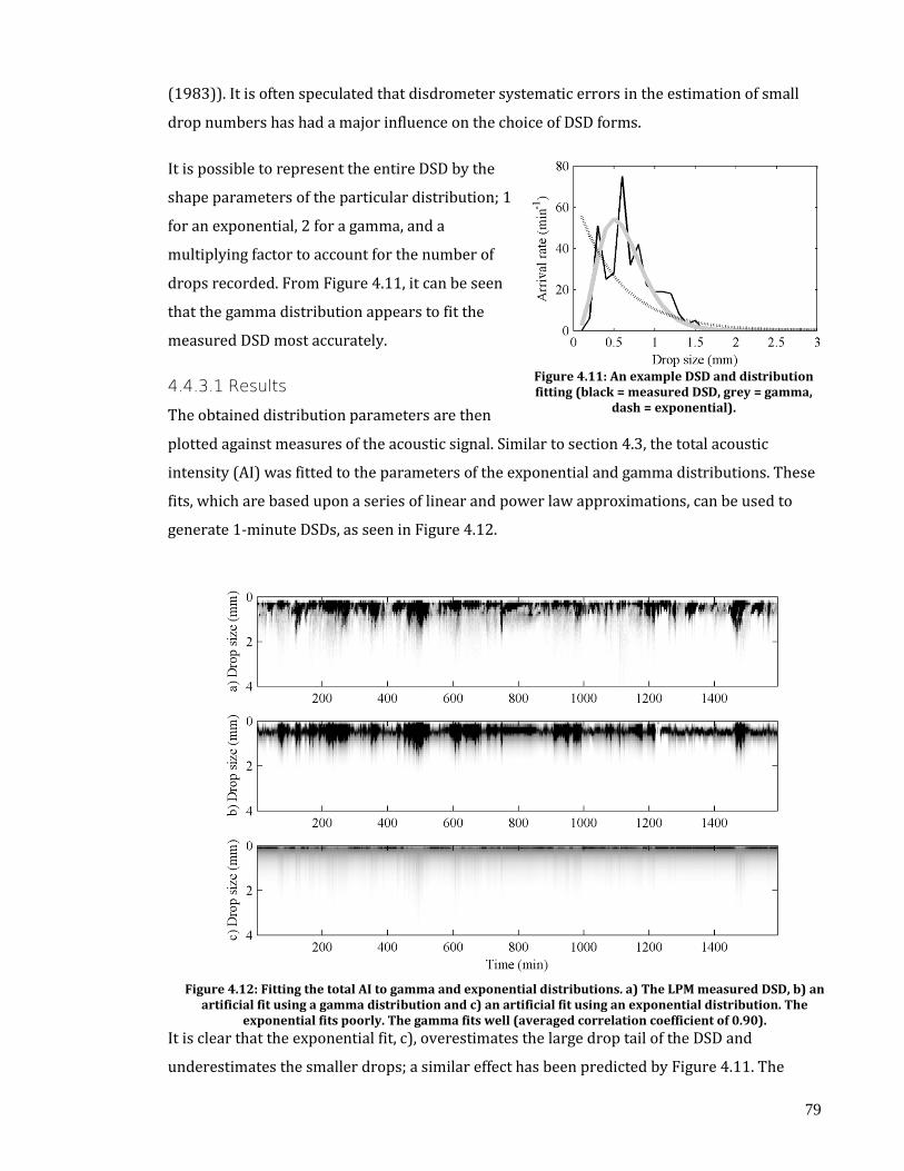
79

(1983)). It is often speculated that disdrometer systematic errors in the estimation of small

drop numbers has had a major influence on the choice of DSD forms.

It is possible to represent the entire DSD by the

shape parameters of the particular distribution; 1

for an exponential, 2 for a gamma, and a

multiplying factor to account for the number of

drops recorded. From Figure 4.11, it can be seen

that the gamma distribution appears to fit the

measured DSD most accurately.

4.4.3.1 Results

The obtained distribution parameters are then

plotted against measures of the acoustic signal. Similar to section 4.3, the total acoustic

intensity (AI) was fitted to the parameters of the exponential and gamma distributions. These

fits, which are based upon a series of linear and power law approximations, can be used to

generate 1-minute DSDs, as seen in Figure 4.12.

Figure 4.12: Fitting the total AI to gamma and exponential distributions. a) The LPM measured DSD, b) an

artificial fit using a gamma distribution and c) an artificial fit using an exponential distribution. The exponential fits poorly. The gamma fits well (averaged correlation coefficient of 0.90).

It is clear that the exponential fit, c), overestimates the large drop tail of the DSD and

underestimates the smaller drops; a similar effect has been predicted by Figure 4.11. The

Figure 4.11: An example DSD and distribution fitting (black = measured DSD, grey = gamma,

dash = exponential).

80

gamma fit, b), looks to fit the measured DSD well, with the effect of smoothing the DSD. This

can be expected as a result of fitting an approximation. Local variations around the

approximation are the largest source of error. For the particular example in Figure 4.11, a

mediocre correlation coefficient of 0.69 is obtained when fitting to a gamma distribution. This

is due to the variance within the LPMs DSD data which is chiefly caused by the small

catchment area (see §4.2.1). However, after averaging over all measured and gamma fitted

DSDs (i.e. the average of all the DSD data in Figure 4.12), the correlation coefficient increases

to 0.90. Again, Nystuen (2001) has found that correlation coefficients for standard commercial

instruments yield between 0.79 and 0.94 which indicates that over a long period of time that a

total acoustic pressure-derived DSD is as accurate as other disdrometers.

4.5 Conclusions Eight months of rain data has been collected and empirical relationships between the energy

in the acoustic sound field within the tank and rain parameters such as intensity and kinetic

energy have been established. Comparisons between rain intensity and kinetic energy

measured by a commercial instrument and those derived from tank measurements are more

highly correlated than comparisons between pairs of commercial instruments. Furthermore,

the new acoustic instrument has been theoretically shown to be able to provide

measurements with an integration time as short as one second. Time-series of one-second

variation in rain parameters have shown a factor of five variations around one-minute

averages.

An investigation into the effect of wind has been described, which showed that only high wind

speed events (average greater than 1.5 m s-1) can significantly affect the results. In the

presence of wind, the KE of smaller drop sizes are increased dramatically, although the

contribution to the overall KE is still low when compared to larger drops. This is because the

KE of a drop is proportional to the fifth power of the diameter (see §2.1.2.1).

Fitting the acoustic intensity data to parameters of a gamma distribution yielded good

correlation coefficients when compared to the LPM provided DSDs. However, the fit is

significantly affected by the variance of the large drop tail of the LPM DSD upon shorter

integration periods.

81

Chapter 5: Entrainment noise

5.1 Introduction Continuing from section 2.2.3.1, entrainment poses as a significant noise source within the

AWTD. The bubbles created as a result of the entrainment process often have a great deal

more power than the impact pulse. It is important to suppress entrainment noise to reduce

errors within the tank.

To reiterate, entrainment is the process where air is forced into a liquid medium, typically

water. This occurs within a rain storm when large drops push air in front of the drop into the

water or when the cavity created by a smaller drop satisfy the conditions of cavity collapse.

The experimental data produced in Figure 2.4 show an example impact and its bubble. For

further information, please refer back to section 2.2.3.

This chapter investigates two possible suppression techniques: altering the liquid properties

to prevent entrainment and using a high powered signal to force the entrained bubbles to

oscillate in a controllable way. Chapter 6 investigates one further and ultimately successful

method of entrainment suppression.

82

5.2 Liquid alteration One possible method of bubble suppression is to alter the liquid’s properties to prevent

entrainment from occurring; i.e. prevent crater formation or provide a cushion to decrease

the chance of entrainment.

It has been shown that bubbles could be suppressed by reducing the surface tension of the

liquid in the tank (Pumphrey et al. (1989)). More recent work investigated how the surface

tension affects entrainment (Deng et al. (2007)). Deng et al. (2007) developed the idea of the

dimensionless capillary number, Ca, which is the measure of the impact velocity, V, with

respect to the viscosity, μ, and the surface tension, σ.

VCa (5.1)

The viscous effects of the liquid had been neglected by most previous studies, but they found

that as this ratio increases the entrained bubble size decreases until Ca ≈ 0.6, when

entrainment no longer occurred. This is partly due to both viscous damping, which decreases

the angle of the crater cone, and by the surface tension, which limits the crater's ability to

pinch-off (i.e. collapse).

5.2.1 Applications to the AWTD Using this principle, it is possible to alter the characteristics of the water in the tank to remove

the source bubble noise. However, the maintenance of such a system could be problematic. If a

surfactant was added to the water, it is likely that the solution would not remain mixed for

extended periods of time and the addition of excess water from rain would further dilute the

mixture. In either case, routine maintenance would be necessary to ensure the correct surface

tension. Another option is to increase the viscosity of the liquid, but after experimentation it

was found that when droplets landed in a similar area in a quick succession, a local pool of

non-viscous water formed and entrainment could subsequently occur.

Furthermore, commonly available surfactants such as washing detergent and washing up

liquid, along with substances such as glycerol tended to form foam bubbles on the surface of

the liquid after a bubble had formed. This surface bubble would then form a cushion for the

next droplet and attenuate the impact signal.

Also when a bubble on the surface popped, it produced several sounds similar to the impact

and entrainment process. Ding et al. (2007) found that acoustic measurements of aqueous

foams show three distinct radiation mechanisms: oscillations of a bubble surface that precede

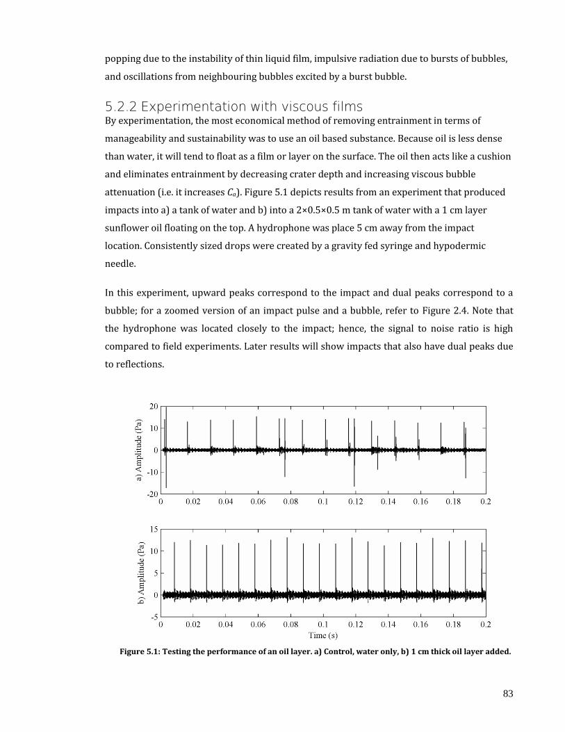
83

popping due to the instability of thin liquid film, impulsive radiation due to bursts of bubbles,

and oscillations from neighbouring bubbles excited by a burst bubble.

5.2.2 Experimentation with viscous films By experimentation, the most economical method of removing entrainment in terms of

manageability and sustainability was to use an oil based substance. Because oil is less dense

than water, it will tend to float as a film or layer on the surface. The oil then acts like a cushion

and eliminates entrainment by decreasing crater depth and increasing viscous bubble

attenuation (i.e. it increases Ca). Figure 5.1 depicts results from an experiment that produced

impacts into a) a tank of water and b) into a 2×0.5×0.5 m tank of water with a 1 cm layer

sunflower oil floating on the top. A hydrophone was place 5 cm away from the impact

location. Consistently sized drops were created by a gravity fed syringe and hypodermic

needle.

In this experiment, upward peaks correspond to the impact and dual peaks correspond to a

bubble; for a zoomed version of an impact pulse and a bubble, refer to Figure 2.4. Note that

the hydrophone was located closely to the impact; hence, the signal to noise ratio is high

compared to field experiments. Later results will show impacts that also have dual peaks due

to reflections.

Figure 5.1: Testing the performance of an oil layer. a) Control, water only, b) 1 cm thick oil layer added.

84

It can be seen that the application of a layer of oil has completely removed the bubble noise

from the signal due to the prevention of crater formation. Only a small loss in the impact

signal was noticed due to viscous absorption. Furthermore, other oils (e.g. engine oil,

lubricating oil) performed equally well indicating that a wide range of oily substances

increase the capillary number to above 0.6.

However, one drawback is that over time, the oil starts to coagulate, reducing the

effectiveness of the film; it would require cleaning and reapplication. Also, at high drop rates

(i.e. many drops impacting a similar area within a small time) a pool of water would be

formed where subsequent drops could generate a bubble due to the entrainment process.

5.3 Driven oscillation The sound generated by the bubble is actually due to the bubble’s oscillation when attempting

to regain hydrostatic equilibrium (§2.2.3.1). As energy is lost and equilibrium approached, the

bubble oscillates in three dimensions pushing and pulling the surrounding water causing far-

field compression waves (i.e. a sound). One idea for suppression is to force the bubble to

oscillate in a way that we can control. This way, we could stimulate the oscillations to occur in

a very small band of frequencies either outside the bands of interest, or at a frequency that is

easily removed from the signal by filtering.

5.3.1 Applications to the AWTD Applying this principle to the acoustic disdrometer, it could be possible to emit a constant

high energy sinusoidal signal into the water tank which will force any entrained bubbles to a

specific frequency. This narrowband frequency can then be filtered via simple signal

processing and the resultant will be a waveform that still holds the impact pulses, but

suppresses the bubbles.

5.3.1.1 Initial experimentation

A hydrophone was placed in a small 0.4×0.3×0.2 m plastic box and attached to a signal

generator via a transformer. The resultant high voltage was able to drive the hydrophone at

pressures upwards of 100 Pa (estimated – at approximately 5 cm) although the electronics

begin to saturate at approximately 45 Pa. Drops that consistently produced bubbles were

created by a gravity fed syringe and hypodermic needle.

Through an initial period of experimentation it became apparent that the inclusion of a high

powered sinusoid did not suppress the bubbles resonant acoustic signal. Only a superposition

85

of the two signals was observed (up to saturation). Figure 5.2 displays the frequency

components of the original, non-forced, impact and entrainment sound (black) and the

inclusion of a forcing signal (red). It can be seen that the addition of a forcing signal has little

effect on the bubbles’ frequencies (peaks between 10 and 20 kHz). The peak at approximately

6 kHz is a resonance of the box.

Figure 5.2: The bubble forcing experimental result reproduced with a logarithmic y scale. The addition of a forcing signal (red) is compared to the original, non-forced, signal (black) in the frequency domain. The addition of a forcing signal has little effect at the bubbles’ frequencies.

5.3.2 A model of an oscillating bubble To verify the results of the experimentation, a theoretical model can be investigated.

An analogy for an oscillating bubble is a mass on a spring. The movement of the mass is

similar to the oscillation of the bubble radius when two incident pressures are straining for

equilibrium. In this case, a bubble could be modelled as a harmonic oscillator which would

describe the motion of the system. This would infer that the system has a resonant frequency

(which can be confirmed by Leighton (1994)). With a further addition, that the system was

damped, this would indicate that the oscillation would tend to equilibrium. It is possible to

derive a model to form the Rayleigh-Plesset equation (Leighton (1994):

)(

4221

2

30

3

0

0

0

2

tPpR

R

Rp

R

Rp

Rp

RRR vv

(5.2)

86

where R0 is the bubble radius at rest, ρ, the fluid density, σ, the surface tension, κ, the specific

heat ratio, η, the shear viscosity, p0, the ambient pressure, pv, the vapour pressure, P(t), a time

varying external pressure and R, R , R are derivatives of the radius with respect to time ▲

which are to be solved numerically.

From (2.1), it can be seen that an external pressure, P(t), can be applied to force the bubble to

oscillate in a way other than its resonance. This occurs naturally upon bubble formation as the

crater collapse, or a pushing drop, provides the bubble with a jolt of energy to initiate

oscillating in accordance to (2.1). Using a modified version of the Rayleigh-Plesset equation to

include an empirically derived damping factor, it is possible to model this process as it occurs

in our freshwater tank (c.f. Figure 5.3). Image a) simulates the bubble formation event and

image b) shows the response in terms of, R, its radius of the created bubble.

Figure 5.3: A numerical solution to a modified version of equation (5.2), simulating bubble creation and

oscillation. a) the driving impulse (i.e. crater collapse and initial compression) and b) the resulting bubble oscillation, in terms of R.

Figure 5.4 depicts a similar simulation whereas now a fixed amplitude external AC driving

pressure is present during the creation and decay of the bubble. Image a) is the driving signal

added to the bubble creation event and b) shows the response of the bubble. Initially, it was

expected that the bubble should first go through a transient period before aligning itself to the

driving oscillation. However, from Figure 5.4 b) it can be seen that there is no significant

effect, apart from a superposition of the two signals.

87

Figure 5.4: Simulating bubble formation and oscillation when exposed to a driving sound field. As Figure

5.3.

Further frequency analysis of the signal (c.f. Figure 5.5) shows that there is no reduction in the

frequency spectrum of the signal, only a superposition.

Figure 5.5: The normalised frequency spectrum of Figure 5.3 b) (solid line) and Figure 5.4 b) (dashed line).

5.3.3 Bubble forcing conclusions The experimental and theoretical results both agree that the bubble forcing method will not

suppress entrainment noise.

88

It is possible to use this method to induce cavitations within a bubble, as shown by Leighton

(1994), however the result would produce spurious harmonics which would further increase

the bubble noise. Furthermore, the required driving signal would have to be very high in

power to ensure adequate driving forces, which would require the acoustic system to have an

extremely high dynamic range. Impact pulses commonly have pressure amplitudes of the

order of 1 Pascal. When Leighton (1994) performed similar experiments, he used pressures of

0.24MPa. To prevent saturation in any amplifiers, a dynamic range greater than 120dB would

be required. Although, an in-line passive filter could be placed before the first amplifier to

filter the appropriate frequencies before they enter the amplification chain. There will,

however, be problems regarding the high impedance of the hydrophone.

5.4 Summary This chapter has considered two different approaches available for impact detection in the

presence of entrainment noise. Two physical methods of entrainment suppression have been

investigated, which attempted to suppress bubble production or to control the frequency of

oscillation of the bubbles that were produced.

The first method was successful in suppressing entrainment. By adding an oil layer to the top

of the water tank it was possible to create a cushion for the impact, which limited crater

formation. Without a crater, entrainment could not occur, thus removing all sources of

entrainment noise. Practical considerations yielded the idea unusable. Oil will coagulate with

time, promote organic growth and subsequent impacts lead to localised pools of water above

the oil layer, which would in turn become a site where entrainment is again possible.

The second projected a high powered sinusoidal pressure wave into the area surrounding an

entrainment site. It was hoped that the bubble will be forced to align its resonance with the

impinging sinusoid and the carrier signal, along with the bubble oscillation, could be filtered

to remove all signs of bubble noise. Unfortunately, theoretical and practical considerations

forced the idea to be abandoned.

With these methods rejected, it became necessary to attempt to filter the signals within the

confines of a software environment. This is considered in chapter 6.

89

Chapter 6: Impact filtering

The most flexible form of bubble noise suppression is via the use of digital signal processing

methods. Inherently, software based analysis’ provide a controlled environment to rapidly

examine and test a multitude of methodologies. The objective of the software is to distinguish

impacts from entrainment noise and estimate drop parameters (i.e. the drop size). This

chapter discusses the methods utilised in order to create an impact impulse detection

algorithm.

Section 6.1 examines the possible sources of noise and analyses the impact and entrainment

signals to identify any distinguishing features. Section 6.2 introduces and describes the

methods of filtering unwanted signals, whilst retaining the impact signal (i.e. impact filtering),

while section 6.3 discusses their implementation. Section 6.4 presents the results of a

comparison between the established impact filters and provides recommendations on which

filter to use in the final direct interpretation routines.

90

6.1 Introduction This section investigates the possible noise sources and discusses the features of the impact

and entrainment signal. Using these findings, several different filtering schemes will be

designed and compared in later sections.

6.1.1 Sources of noise In order to filter everything but the impact signal, we must consider other signals which the

system considers to be noise. Entrainment noise has already been established as the major

source, but others may also contribute to a lesser degree.

The electrical noise caused by other equipment or power sources can enter the system to

increase overall noise levels. Inadequate power supply filtering often allows a small amount of

mains ripple on to the DC power lines within the circuit. This signal is then internally

amplified along with the desired signal and presented at the output as noise. Furthermore,

switching transients, where other systems suddenly require large amounts of current (e.g.

switching a light on), cause a near instantaneous (i.e. broadband) drop in voltage (due to the

resistance of the power lines) which again can transfer to the DC power rails within a system.

The proliferation of switching power supplies only adds to this problem.

The majority of the mains noise occurs at its fundamental frequency of 50 Hz. However,

spurious transients can produce harmonics up to 50 kHz. Hence, it is necessary to filter the

pre-amplifier’s DC power lines before the amplifiers. The LC combination filters on the power

lines in the schematic (c.f. Figure 3.13) provide a suitable amount of filtering; any noise picked

up from the hydrophone cables is largely unavoidable. The remaining 50 Hz mains noise and

wind induced oscillations of the tank can be filtered via signal processing methods with a

simple high pass filter. This also has the benefit of blocking the DC component of the signal

which can arise from DC amplification errors.

Several studies have investigated the sound produced by wind at sea (e.g. Vagle et al. (1990),

Ma et al. (2005)) allowing the measurement of wind speed from acoustic data. However, the

AWTD’s body of water is much smaller, and the wind speeds are generally lower due to wind

shielding around the AWTD site. However, the HDPE (high density polyethylene) walled tank

is fairly thin; approximately 1-2 mm. This does not provide the structural rigidity to hold the

tank in place during high winds. Instead it tends to flex and distort.

From experimentation, the wind signal has frequency components up to 1 kHz which depend

on wind speed and resonances of the tank structure (this includes the hydrophone cables). A

91

cut off frequency of 1 kHz was chosen, which adequately filters most of the mains and wind

noise.

6.1.2 A detailed look at an impact signal From chapters 2 and 5, it was found that each bubble size has a corresponding resonant

frequency. This implies that it may be possible to filter out signals within this frequency range

by simple notch filters.

6.1.2.1 The frequency components of the impact process

The range of frequencies contained in the distribution bubble resonances are often cited as

anywhere between 14-16 kHz (Pumphrey et al. (1989) and 1.8-21 kHz (Medwin et al. (1992)).

Clearly the width of the spectral peak due to entrainment is dependent on the threshold

chosen by the author; however, the difference in ranges is large. It is more likely that Medwin

et al. (1992) is correct, since the distribution of entrained bubble sizes can vary widely, which

in turn is dictated by the DSD.

In laboratory conditions, the bubble size is usually constrained by the size of the impacting

drop. Medwin et al. (1992) also found bubble frequencies extending to 30 kHz (Fig. 6 – in

Medwin et al. (1992)), which occurred for 5% of the time for large drops (i.e. 1 in 20); in the

presence of thousands of drops per second, this is fairly likely. Furthermore, it is also likely

that frequencies above 30 kHz could be produced, albeit less often.

To visualise the frequency components of an impact and bubble, consider an example event as

in Figure 6.1. Image a) presents a graph of the signal received at a single hydrophone. There

are 3 distinct parts of the signal. At approximately 16 ms and impact occurs, which is shown in

Figure 6.2, then at approximately 200 ms a bubble is produced, Figure 6.3. There is also a

subsequent smaller impact at 275 ms. Note that this is taken from the final AWTD tank, hence

the depth of the hydrophone has increased and subsequently the SNR has decreased. For

example, the pulses after the initial upwards pulse of the impact are reflections.

Image b) in Figure 6.1 displays the short time Fourier transform (also known as the Gabor

transform) which computes the FFT over short time segments to yield a graph of the FFT over

time. In this particular case (others will differ), the two impacts consist of frequencies up to

approximately 25-30 kHz. It is clear that the bubble also contains frequencies up to 30 kHz,

but of a much higher power. This initial high frequency is due to the sound of capillary waves

inside the crater colliding at the instant between crater collapse and bubble formation.

92

Figure 6.1: A short time fast Fourier transform of an impact and bubble.

Figure 6.2: A zoomed version of Figure 6.1 (impact)

Figure 6.3: A zoomed version of Figure 6.1 (bubble)

6.1.2.2 Consequences

The results of section 6.1.2.1 have established that simple notch or high-pass filters are

unusable since bubbles and impacts contain similar frequency components. Furthermore,

even if an impact did range to a slightly higher frequency, (e.g. 50 kHz), it would still be

unwise to filter frequencies, since a significant amount of impact energy lies within the lower

part of the spectrum. This would lower the impact pulse-to-noise ratio to the point where

detection may no longer be possible; more sophisticated filtration methods are required.

93

6.1.3 Discriminating an impact by its shape Since a simple frequency discriminating filter will not work, we must investigate other

methods that utilise the subtle differences between the impact and bubble signals.

6.1.3.1 Time domain impact-bubble comparison

Several features can be seen in the time domain characteristics of an ideal impact and bubble

(c.f. Figure 6.4). Often, before an impact or bubble event, the signal is be zero (i.e. below the

noise floor - feature A). Feature B shows an ideal impact that is a band-limited impulse. Also

note the short amount of relaxation oscillation that is due to resonances within the

hydrophone. Dependant on the size of the impact, this signal could be masked by reflections

off the bottom and sides of the tank (which would be totally absorbed if the lining was fully

anechoic). Feature C displays a perfectly sinusoidal decaying bubble. Comparing features B

and C, we can see that:

the impact is of short duration, the bubble is of long duration

the first portion of the oscillation in the impact is positive, the bubble’s is negative

- The impact is positive due to the compressive force of the impact. The bubble

is negative due to the decompressive force of the upwards collapse of the

crater.

a single period of the bubble looks similar to an impact

the bubble often contains more power than the impact

Utilising these features, it is possible to design a filter that can distinguish between an isolated

impact and a bubble signal.

Figure 6.4: An ideal impact and bubble signal.

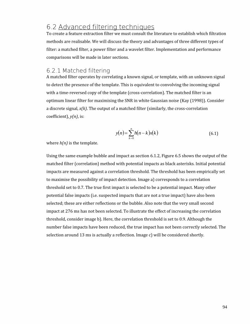
94

6.2 Advanced filtering techniques To create a feature extraction filter we must consult the literature to establish which filtration

methods are realisable. We will discuss the theory and advantages of three different types of

filter: a matched filter, a power filter and a wavelet filter. Implementation and performance

comparisons will be made in later sections.

6.2.1 Matched filtering A matched filter operates by correlating a known signal, or template, with an unknown signal

to detect the presence of the template. This is equivalent to convolving the incoming signal

with a time-reversed copy of the template (cross-correlation). The matched filter is an

optimum linear filter for maximising the SNR in white Gaussian noise (Kay (1998)). Consider

a discrete signal, x(k). The output of a matched filter (similarly, the cross-correlation

coefficient), y(n), is:

n

k

kxknhny0

(6.1)

where h(n) is the template.

Using the same example bubble and impact as section 6.1.2, Figure 6.5 shows the output of the

matched filter (correlation) method with potential impacts as black asterisks. Initial potential

impacts are measured against a correlation threshold. The threshold has been empirically set

to maximise the possibility of impact detection. Image a) corresponds to a correlation

threshold set to 0.7. The true first impact is selected to be a potential impact. Many other

potential false impacts (i.e. suspected impacts that are not a true impact) have also been

selected; these are either reflections or the bubble. Also note that the very small second

impact at 276 ms has not been selected. To illustrate the effect of increasing the correlation

threshold, consider image b). Here, the correlation threshold is set to 0.9. Although the

number false impacts have been reduced, the true impact has not been correctly selected. The

selection around 13 ms is actually a reflection. Image c) will be considered shortly.

95

Figure 6.5: Using the matched filter method on an example impact and bubble signal. a) Correlation coefficient set to 0.7. b) Correlation coefficient set to 0.9. c) Matched filter post-processing applied.

Potential impacts are black asterisks.

6.2.1.1 Matched filter post-processing

One method of attempting to remove the erroneous impacts is by looking at the data

surrounding the potential impact.

96

The matched filter will only generate a potential impact if the correlation coefficient is greater

than 0.7 (in this example). With references to Figure 1.4, the initial cycle of a bubble is always

negative (i.e. decompressive), only subsequent cycles could possibly be impacts. Therefore, it

is possible to check the amount of RMS amplitude around an isolated potential impact (i.e. the

RMS average over several samples – set to approximately 2 periods at 17 kHz, 0.1 ms). The

ratio between the potential impact amplitude and the RMS amplitude is compared to a

threshold (set to 2.25 – chosen empirically). If the impact-to-RMS amplitude ratio is greater

than the threshold then it can be considered as a potential impact (also see §6.2.2: Filtering by

power). Let us examine a few examples:

1. Upon a bubble event, the RMS amplitude of a bubble will be high = no detect.

2. Upon a real impact, the RMS amplitude before and after an impact is ideally zero =

detect.

3. When two subsequent real impacts occur, the RMS amplitude within both impacts is

still relatively small (dependant on size of impacts – a small impact after a very large

impact may not detect); as large drops are fairly rare = usually detect both.

4. Upon a real impact within a bubble, the RMS amplitude within a bubble will be high =

no detect (unless the impact amplitude is much greater than the bubble).

Only criterion 4 leads to errors. This is a major limiting factor for this and other methods.

However, we are mainly interested in larger drops, which should generally provide a greater

signal amplitude for possible detection; the loss of several small drops inside a bubble is

unfortunate, but possibly acceptable. Furthermore, spatial filtering (§7.1.3) could be utilised

to provide a ‘best guess’ in situations such as these.

Referring back to Figure 6.5, image c) is the result of this method. It is clear that the number of

false impacts has reduced and the true impact has been detected. However, the number of

false detects is still high.

6.2.2 Filtering by power Section 6.1.3.1 and 6.2.1.1 speculated that the bubble contains considerably more power than

an impact. As an example, the RMS amplitude of the impact and bubble of image Figure 6.1

was calculated where only data that was above a noise threshold were used (approximately 4

standard deviations - 0.05 Pa, above the mean). The impact was calculated to have an average

root-mean-square (RMS) amplitude of 0.14 Pa, whereas the bubble has 0.35 Pa. Taking the

duration of each signal into account yields a ratio of impact energy to bubble energy of

approximately 1:16. We could use this to filter out all components that have a large average

97

RMS amplitude. To estimate the power within the impact and bubble signals, there are two

options: calculating the time-averaged RMS pressure or using the Hilbert transform.

6.2.2.1 Root-mean-square (RMS) method

The RMS amplitude of a signal is usually computed over a set period or window. We need to

select a period that will ensure that the bubbles, with typical frequencies between 10 and 30

kHz, will yield a high average RMS amplitude. By selecting a period that is too small, the RMS

amplitude will only be calculated over a single period of a bubble’s sinusoidal signal. Selecting

a period that is too high and the temporal resolution is decreased.

Figure 6.6: An example calculation of the RMS pressure of a bubble (black = bubble signal, blue = 2

samples, red = 12 samples, green = 24 samples, yellow = 120 samples).

Figure 6.6 shows an example RMS calculation of a bubble. It can be seen that averaging

periods of 2 samples (blue) and 120 samples (green) yield a poor representation of the power

contained within a typical bubble signal. Selecting an averaging period equal to that of

approximately one cycle of a bubble (considering bubble frequencies of 10-30 kHz), a period

of 0.06 ms (12 samples) was chosen (since the majority of bubbles occur in the 10-20 kHz

range).

6.2.2.2 Hilbert transform method

The Hilbert transform operates on a real function, u(t), and produces another real function,

H(u(t)). It is utilised in many applications including: modulation, data analysis and signal

processing. Often, it is used to derive the analytic representation of a signal and can be

thought of representing the function u(t) with its positive frequency components shifted by -

90° in phase and negative frequency components shifted by +90°. The resultant is a signal that

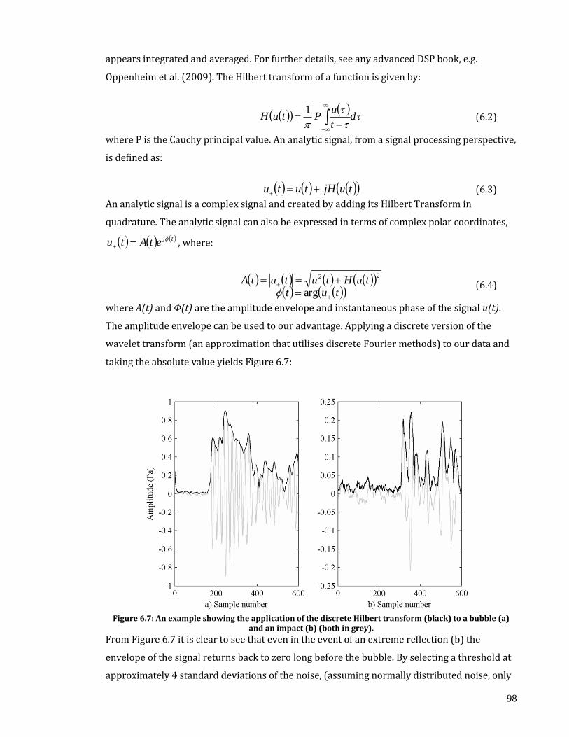
98

appears integrated and averaged. For further details, see any advanced DSP book, e.g.

Oppenheim et al. (2009). The Hilbert transform of a function is given by:

d

t

uPtuH

1

(6.2)

where P is the Cauchy principal value. An analytic signal, from a signal processing perspective,

is defined as:

tujHtutu (6.3)

An analytic signal is a complex signal and created by adding its Hilbert Transform in

quadrature. The analytic signal can also be expressed in terms of complex polar coordinates,

tjetAtu , where:

tut

tuHtututA

arg

22

(6.4)

where A(t) and Φ(t) are the amplitude envelope and instantaneous phase of the signal u(t).

The amplitude envelope can be used to our advantage. Applying a discrete version of the

wavelet transform (an approximation that utilises discrete Fourier methods) to our data and

taking the absolute value yields Figure 6.7:

Figure 6.7: An example showing the application of the discrete Hilbert transform (black) to a bubble (a)

and an impact (b) (both in grey).

From Figure 6.7 it is clear to see that even in the event of an extreme reflection (b) the

envelope of the signal returns back to zero long before the bubble. By selecting a threshold at

approximately 4 standard deviations of the noise, (assuming normally distributed noise, only

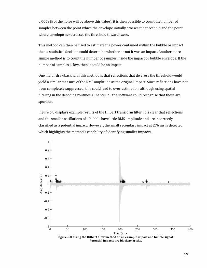
99

0.0063% of the noise will be above this value), it is then possible to count the number of

samples between the point which the envelope initially crosses the threshold and the point

where envelope next crosses the threshold towards zero.

This method can then be used to estimate the power contained within the bubble or impact

then a statistical decision could determine whether or not it was an impact. Another more

simple method is to count the number of samples inside the impact or bubble envelope. If the

number of samples is low, then it could be an impact.

One major drawback with this method is that reflections that do cross the threshold would

yield a similar measure of the RMS amplitude as the original impact. Since reflections have not

been completely suppressed, this could lead to over-estimation, although using spatial

filtering in the decoding routines, (Chapter 7), the software could recognise that these are

spurious.

Figure 6.8 displays example results of the Hilbert transform filter. It is clear that reflections

and the smaller oscillations of a bubble have little RMS amplitude and are incorrectly

classified as a potential impact. However, the small secondary impact at 276 ms is detected,

which highlights the method’s capability of identifying smaller impacts.

Figure 6.8: Using the Hilbert filter method on an example impact and bubble signal.

Potential impacts are black asterisks.

100

6.2.3 Wavelet filtering The wavelet transform is analogous to Fourier techniques, applied locally, so that frequency

information is available as a function of time. Wavelet transforms are more applicable to non-

stationary signals as they can provide spectral approximations from short intervals, unlike

Fourier analysis which averages over the whole of the signal. Consider the example of a unit

impulse function with infinite bandwidth. The wavelet transform can represent this short-

term signal with only a few terms. Impact and bubble sounds are both intermittent with

durations of tens of microseconds and milliseconds respectively.

Wavelets provide a method of viewing a time-series over multiple resolutions, where each

finer resolution includes information at higher frequencies. The technique takes averages and

differences of a signal over a hierarchy of intervals that are analogous to spectrum

wavelengths. The average and differencing operations are performed over a window and then

shifted. There are an infinite number of possible windows, but some provide properties that

are more advantageous for a particular application. For example, Haar windows are

conceptually simple, fast and exactly invertible. However, as they are not overlapped, high

frequency information visible in lower level (frequency) wavelets can be neglected in higher

levels of decomposition. A Daubechies or Meyer window can provide overlapping averaging

to yield accurate high frequency components at an increased computational cost. However, it

is crucial to note that the calculation of wavelet coefficients is dependent on the correlation

between the mother wavelet and signal of interest (Rafiee et al. (2009)).

Further introductory information can be found in Walker (1999), Weeks (2010) or Ogden

(1997). Further introductions can also be found on the internet at Polikar (2010) and Kaplan

(2010).

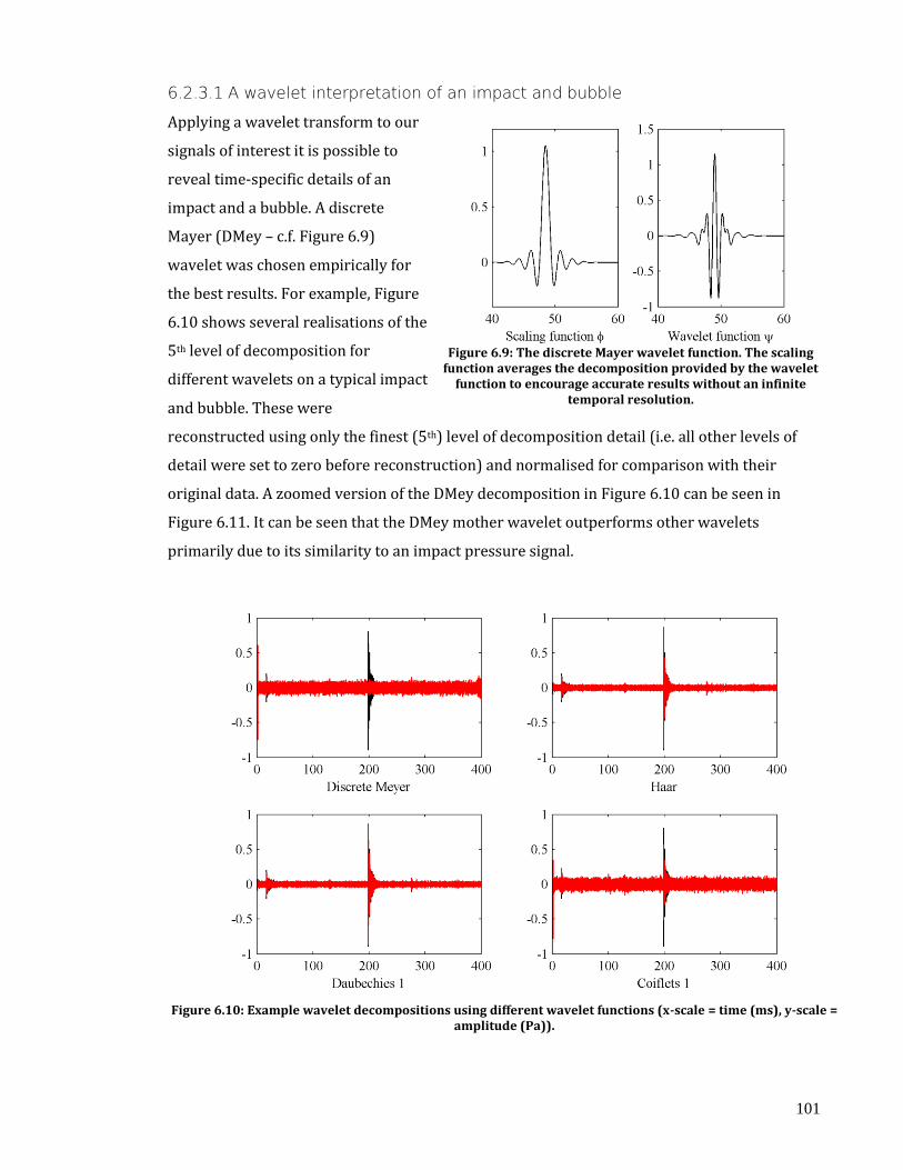
101

6.2.3.1 A wavelet interpretation of an impact and bubble

Applying a wavelet transform to our

signals of interest it is possible to

reveal time-specific details of an

impact and a bubble. A discrete

Mayer (DMey – c.f. Figure 6.9)

wavelet was chosen empirically for

the best results. For example, Figure

6.10 shows several realisations of the

5th level of decomposition for

different wavelets on a typical impact

and bubble. These were

reconstructed using only the finest (5th) level of decomposition detail (i.e. all other levels of

detail were set to zero before reconstruction) and normalised for comparison with their

original data. A zoomed version of the DMey decomposition in Figure 6.10 can be seen in

Figure 6.11. It can be seen that the DMey mother wavelet outperforms other wavelets

primarily due to its similarity to an impact pressure signal.

Figure 6.10: Example wavelet decompositions using different wavelet functions (x-scale = time (ms), y-scale =

amplitude (Pa)).

Figure 6.9: The discrete Mayer wavelet function. The scaling

function averages the decomposition provided by the wavelet function to encourage accurate results without an infinite

temporal resolution.

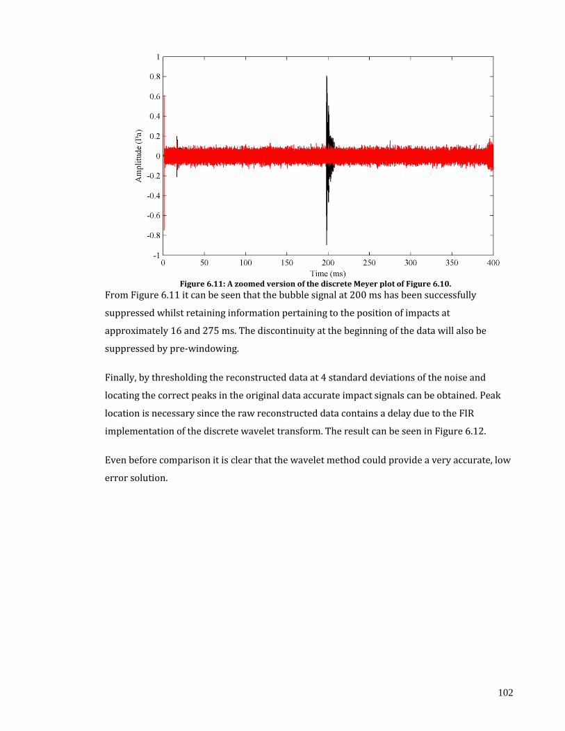
102

Figure 6.11: A zoomed version of the discrete Meyer plot of Figure 6.10.

From Figure 6.11 it can be seen that the bubble signal at 200 ms has been successfully

suppressed whilst retaining information pertaining to the position of impacts at

approximately 16 and 275 ms. The discontinuity at the beginning of the data will also be

suppressed by pre-windowing.

Finally, by thresholding the reconstructed data at 4 standard deviations of the noise and

locating the correct peaks in the original data accurate impact signals can be obtained. Peak

location is necessary since the raw reconstructed data contains a delay due to the FIR

implementation of the discrete wavelet transform. The result can be seen in Figure 6.12.

Even before comparison it is clear that the wavelet method could provide a very accurate, low

error solution.

103

Figure 6.12: Output from wavelet detection routine for an example impact and bubble. a) and b) are

zoomed images of the impacts at 16 and 275 ms, respectively.

6.2.4 Other filtering possibilities From chapter 2, it was established that other authors have previously attempted to solve the

impact detection problem. Mani and Pillai (2004) proposed a solution by attempting to find

the approximate derivative (by differencing) of the signal. The difference of an ideal one sided

impulse is equal to a two sided impulse. Hence, all impacts, which are ideally impulse-like, will

remain largely untouched whilst the bubble signals will be significantly reduced. However, we

know that the impacts are not ideal and contain a significant amount of low frequency

content. Differencing will therefore reduce the magnitude of the impact as well as the bubble.

Since the impact is usually much smaller in amplitude, the net effect is the opposite of that

desired: the impact signal is reduced beneath the noise floor (and therefore indistinguishable)

whereas the bubble signal is only slightly damped. This is clearly counter-productive.

6.3 Filter implementation This section describes the computational implementation of the filtration routines. The

objective is to identify the best method to be assimilated into the direct interpretation

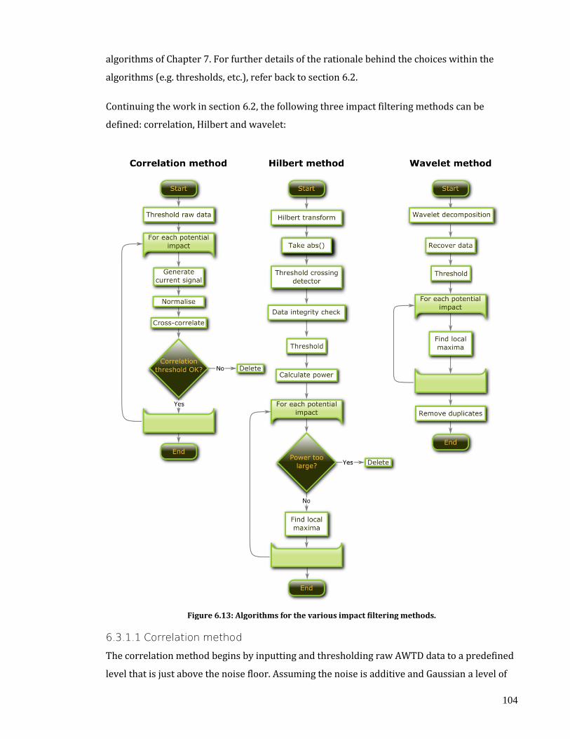
104

algorithms of Chapter 7. For further details of the rationale behind the choices within the

algorithms (e.g. thresholds, etc.), refer back to section 6.2.

Continuing the work in section 6.2, the following three impact filtering methods can be

defined: correlation, Hilbert and wavelet:

Figure 6.13: Algorithms for the various impact filtering methods.

6.3.1.1 Correlation method

The correlation method begins by inputting and thresholding raw AWTD data to a predefined

level that is just above the noise floor. Assuming the noise is additive and Gaussian a level of

105

approximately 4 standard deviations has been chosen that will be exceeded by chance with a

probability of only 0.0063%. Each individual point above the threshold is compared to an

idealised impact pulse generated from the average of approximately 100 drops. If the

resulting correlation coefficient is above another preset threshold (set to 0.7) then it is

considered to be a valid drop.

6.3.1.2 Hilbert method

The Hilbert method, named for its use of the Hilbert transform, uses the lack of power

contained within an impact when compared to a bubble. It starts by inputting raw data and

performing a Hilbert transform. The modulus of the returned complex data is then passes

through a threshold crossing detector. After finding potential impacts, the RMS amplitude of

each potential impact interval is calculated. Each result is then compared against another

preset threshold, based upon the information in section 6.2.2, of 0.2 Pa. If the RMS amplitude

of any particular event is too large, it is discarded. Since the threshold crossing detector only

returned information on the boundary of each area, the data within the area is then searched

for the maximum peak, which is assumed to be the impact.

6.3.1.3 Wavelet method

The wavelet method accepts raw data and performs wavelet decomposition. Using only the

higher coefficients proved to be a successful method of drop detection and, after

reconstruction, yields a raw signal with a very low incidence and amplitude of bubble signal

(see §6.2.3). Comparing the reconstructed data to a threshold at 4 standard deviations obtains

a set of potential impact locations. Finally we must locate the peak due to delays introduced

by the implementation of the discrete wavelet transform.

6.4 Filter comparison In this section we compare the performance of the three designed impact filters to decide

which is the most suitable to use in the final direct interpretation algorithm of Chapter 7.

The results of such a comparison will be discussed with the investigation of the types and

sources of errors. Several examples of errors found within the data are also reproduced to aid

understanding.

6.4.1 Methodology To compare the performance of the three impact filters, several sets of raw data are analysed

by hand to count the number and locations of signals that I consider to be impacts. It is

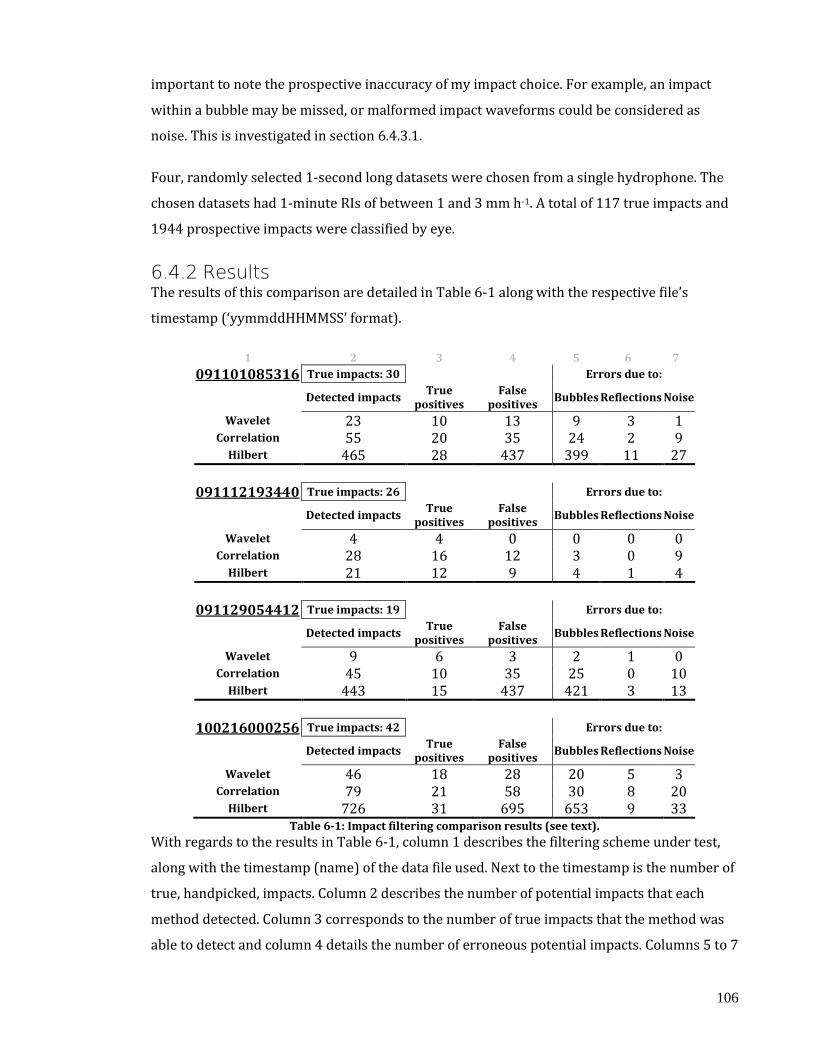
106

important to note the prospective inaccuracy of my impact choice. For example, an impact

within a bubble may be missed, or malformed impact waveforms could be considered as

noise. This is investigated in section 6.4.3.1.

Four, randomly selected 1-second long datasets were chosen from a single hydrophone. The

chosen datasets had 1-minute RIs of between 1 and 3 mm h-1. A total of 117 true impacts and

1944 prospective impacts were classified by eye.

6.4.2 Results The results of this comparison are detailed in Table 6-1 along with the respective file’s

timestamp (‘yymmddHHMMSS’ format).

1 2 3 4 5 6 7

091101085316 True impacts: 30 Errors due to:

Detected impacts True

positives False

positives Bubbles Reflections Noise

Wavelet 23 10 13 9 3 1 Correlation 55 20 35 24 2 9

Hilbert 465 28 437 399 11 27

091112193440 True impacts: 26 Errors due to:

Detected impacts True

positives False

positives Bubbles Reflections Noise

Wavelet 4 4 0 0 0 0 Correlation 28 16 12 3 0 9

Hilbert 21 12 9 4 1 4

091129054412 True impacts: 19 Errors due to:

Detected impacts True

positives False

positives Bubbles Reflections Noise

Wavelet 9 6 3 2 1 0 Correlation 45 10 35 25 0 10

Hilbert 443 15 437 421 3 13

100216000256 True impacts: 42 Errors due to:

Detected impacts True

positives False

positives Bubbles Reflections Noise

Wavelet 46 18 28 20 5 3 Correlation 79 21 58 30 8 20

Hilbert 726 31 695 653 9 33 Table 6-1: Impact filtering comparison results (see text).

With regards to the results in Table 6-1, column 1 describes the filtering scheme under test,

along with the timestamp (name) of the data file used. Next to the timestamp is the number of

true, handpicked, impacts. Column 2 describes the number of potential impacts that each

method detected. Column 3 corresponds to the number of true impacts that the method was

able to detect and column 4 details the number of erroneous potential impacts. Columns 5 to 7

107

show how many erroneous impacts correspond to a particular type of error: bubble,

reflection and noise errors.

Bubble error: the impact filter decides a bubble is an impact

Reflection error: the impact filter decides a reflection is an impact

Noise error: the impact filter decides anything else is an impact. (e.g. random noise,

irregular spikes, irregular bubble shapes, etc.)

1 2 3 4 5 6 7

Average percentile error Average error due to: True detect False detect Reported error Bubble Reflections Noise

Correlation 57% 68% +77% 59% 7% 34% Hilbert 74% 95% +1315% 93% 2% 5%

Wavelet 32% 54% -30% 71% 20% 9% Table 6-2: Average errors presented as percentiles (see text).

Table 6-2 displays the results of Table 6-1 as a percentage of several different errors. Column

1 describes the filtering method under test. Column 2 presents the average percentage of

impacts that each method correctly detected. Column 3 shows the average percentage of false

detects. Column 4 reports the average estimation of the total number of drops. Columns 5 to 7

show the average percentage error associated with each error type.

6.4.3 Discussion The aim of this section is to establish which impact filtering method is the best at providing

consistent, accurate results. Performing an analysis of the results from section 6.4.2, we can

see that there are several interesting results.

Referring to the averaged results of Table 6-2, there is a correlation between the percentage

of true detects and the total number of potential impacts (reported error). As one might

expect, when a large amount of potential impacts are generated, the number of true impacts

will typically increase. This effect can be seen in the Hilbert transform method of filtration.

The key metric is the reported error. This is the percentage that each method’s potential

impact number is above or below the true number of impacts. For example, the correlation

method reported 77% more drops than the true value, on average. Using this it is clear to see

that the wavelet method of filtration produces the least error, although it also detects the least

amount of true impacts.

The wavelet method of filtration is the most robust (i.e. it produces less errors), however it

does underestimate the total true impact population (-30%). This could be improved during

the impact decoding routines of Chapter 7, which use multilateration to predict and located

108

other missing impacts. False-positive impact identifications can be eliminated from the

dataset when they correspond to drops that impact outside the tank. This error-correction

mechanism leads to more accurate final results than would be expected from the over-

estimation of impacts at this stage. This can be seen in the final estimated DSD in Section 7.4.

It is also interesting to note that the majority of errors were due to bubbles. This is as

expected. It can also be seen that different methods are more susceptible to different types of

error. For example, the correlation method is more susceptible to noise (i.e. white Gaussian

noise, impact-like coincidences, etc.), but the wavelet method is more susceptible to reflection

noise (however the wavelet error averages are not reliable as other methods due to the

relative lack of errors).

6.4.3.1 Examples of errors

As an aid to help visualise the reasons why a particular method may produce errors, Figure

6.14 displays several plots of typical error sources. Image a) corresponds to a potential impact

due to noise; some data can look like an impact pulse. Image b) shows an impact occurring

within a bubble. The sinusoidal oscillation of the bubble is clear and, in this instance, it is

relatively easy to see the impact due to the impact being fairly large. It is also possible to see

other potential impacts that the software has missed. Often the impact is small in relation to

the bubble and the impact will go undetected. Image c) shows a bubble that was detected as

an impact. If we look at the size of the downward spike compared to the initial upward spike

and notice the coherent oscillation after the event, I would consider this to be a bubble, not an

impact. This is an example of a non-ideal bubble, since it was found that bubbles usually start

with a downward spike (Figure 6.4).

Figure 6.14: Example of possible filtering errors due to: a) noise, b) impact in bubble, c) bubble that looks

like impact (stars denote possible error locations, raw data in grey).

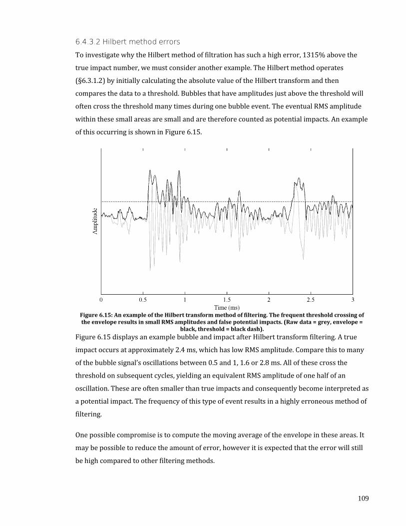
109

6.4.3.2 Hilbert method errors

To investigate why the Hilbert method of filtration has such a high error, 1315% above the

true impact number, we must consider another example. The Hilbert method operates

(§6.3.1.2) by initially calculating the absolute value of the Hilbert transform and then

compares the data to a threshold. Bubbles that have amplitudes just above the threshold will

often cross the threshold many times during one bubble event. The eventual RMS amplitude

within these small areas are small and are therefore counted as potential impacts. An example

of this occurring is shown in Figure 6.15.

Figure 6.15: An example of the Hilbert transform method of filtering. The frequent threshold crossing of the envelope results in small RMS amplitudes and false potential impacts. (Raw data = grey, envelope =

black, threshold = black dash).

Figure 6.15 displays an example bubble and impact after Hilbert transform filtering. A true

impact occurs at approximately 2.4 ms, which has low RMS amplitude. Compare this to many

of the bubble signal’s oscillations between 0.5 and 1, 1.6 or 2.8 ms. All of these cross the

threshold on subsequent cycles, yielding an equivalent RMS amplitude of one half of an

oscillation. These are often smaller than true impacts and consequently become interpreted as

a potential impact. The frequency of this type of event results in a highly erroneous method of

filtering.

One possible compromise is to compute the moving average of the envelope in these areas. It

may be possible to reduce the amount of error, however it is expected that the error will still

be high compared to other filtering methods.

110

6.5 Conclusions This chapter has investigated the possibility of impact detection using signal processing

methods. By a careful consideration of noise sources, it was found that the noise associated

with entrainment was potentially the greatest. In order to investigate different methods of

filtering a detailed analysis of the impact and entrainment signals was performed. It was

found that the bubble and impact signals spanned a similar spectral range. This ruled out

simple frequency-based filtering schemes. Several further techniques utilised the shape of the

impact as a filtering mechanism.

Three different filtering methods have been investigated: matched (correlation), power

(Hilbert) and wavelet. It was found that the wavelet method was the most successful with a

30% underestimation of the true impact population. The Hilbert method performed the worst

due to errors caused by bubble oscillations just crossing a threshold. The correlation method

worked fairly well, although it was highly susceptible to noise.

111

Chapter 7: Direct interpretation

The second major objective of this project was to use the tank and an array of hydrophones to

individually pick out each impacting drop and assign it to a drop size. This way, a direct

conversion from impact sound to DSD would be possible. Ideally this would not assume any

particular form for the DSD e.g. Exponential or Gamma; and results would not rely upon

averaging over the stochastic properties of a large number of impacts.

However, this process ultimately depends on the accuracy of the impact sound-to-drop size

conversion. Since many impacts also produce bubbles, some of the impact energy is diverted

to bubble creation. This has been verified by Medwin et al. (1990). Hence, the conversion of

impact amplitude pressure to drop size becomes a statistical process, as a drop of a particular

size can generate a range of impact pressure amplitudes.

This chapter describes the software algorithms that form the core of the AWTD system when

used to interpret individual impacts. Section 7.1 describes the methods to capture, filter,

inspect and invert the impact sounds to yield drop parameters. Section 7.2 formulates the

methods and mathematics that enable the impact positioning. Section 7.3 describes how

impact pressure can be converted to a drop size and section 7.4 presents the results and

analysis of the entire DSD creation process.

112

7.1 Impact decoding In Chapter 6, we introduced several methods of impact filtering. It was found that the wavelet

method of impact filtering yielded the best results. Using this to remove contamination by

bubble noise, we can extract a set of data (a dataset) that corresponds to the amplitude and

time of arrival (the impact datum) for each potential impact pressure wave, referenced to the

receiving hydrophone. Ideally, a single large impact will generate at dataset containing 4

impact data (one for each hydrophone).

One added complication is due to the size of the tank. Depending on the rainfall intensity and

the catchment area, there is always a chance of the sounds from multiple impacts arriving at a

hydrophone within the same sampling period – i.e. within 5 μs of each other. ‘Near impacts’

are defined as those that occur within the time required for the sound to reach a hydrophone

from the tank extremity, i.e. 0.74 m ≈ 0.5 ms. This assumes that reflected sound waves are

sufficiently attenuated not to be detected as a new drop impact.

To establish an impact location, at least three hydrophones are required. For the prototype

AWTD 4 hydrophones are used to test the utility of redundancy and to aid in the estimation of

drop size. Hence, four individual impact pulses would require detection and decoding to

ensure the correct set of impacts are passed to the drop location and sizing routines.

7.1.1 Impact dataset acquisition A pressure wave generated by a raindrop impacting on the water

surface will propagate through the water and be measured by each

of the four hydrophones. An array containing the arrival times of

the four impacts will be known as an ‘impact dataset’. The relative

timing of these four measurements depends upon the drop impact

position. An impact in the centre of the tank will be measured

simultaneously at all four hydrophones. The maximum time interval

between impact detection at the first and last hydrophones is

limited by the wave propagation time between the most widely

separated hydrophones.

Impact localisation requires identification of the pressure wave generated by an individual

drop impact at each hydrophone. For low rain intensities this is straightforward. However, at

higher rain intensities it is increasingly common for impact arrivals to occur in different

Figure 7.1: Impact dataset

acquisition.

113

orders at each hydrophone. An algorithm is required to sort and identify these arrivals at each

hydrophone.

Due to the known maximum delay between arrivals, hydrophone records are scanned using a

sliding window of approximately 0.5 ms. Impacts more widely separated than this could not

have been generated by the same impact. Furthermore, the amplitude of the wave decreases

with increasing propagation time due to spherical spreading. Therefore, measured impact

pressure wave amplitudes should decrease in temporal order. However, this heuristic isn’t

applied due to errors in peak amplitude estimation and interference between pressure waves.

Finally, if a dataset does not contain impact data from all four hydrophones, an artificial

impact with zero amplitude and time of arrival is added to represent the unknown impact

data; this aids later computation. This process is described in Figure 7.1.

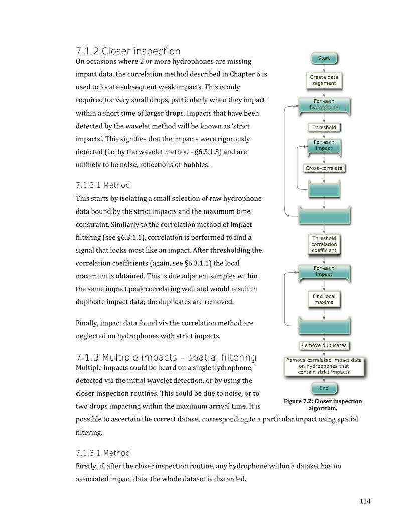
114

7.1.2 Closer inspection On occasions where 2 or more hydrophones are missing

impact data, the correlation method described in Chapter 6 is

used to locate subsequent weak impacts. This is only

required for very small drops, particularly when they impact

within a short time of larger drops. Impacts that have been

detected by the wavelet method will be known as ‘strict

impacts’. This signifies that the impacts were rigorously

detected (i.e. by the wavelet method - §6.3.1.3) and are

unlikely to be noise, reflections or bubbles.

7.1.2.1 Method

This starts by isolating a small selection of raw hydrophone

data bound by the strict impacts and the maximum time

constraint. Similarly to the correlation method of impact

filtering (see §6.3.1.1), correlation is performed to find a

signal that looks most like an impact. After thresholding the

correlation coefficients (again, see §6.3.1.1) the local

maximum is obtained. This is due adjacent samples within

the same impact peak correlating well and would result in

duplicate impact data; the duplicates are removed.

Finally, impact data found via the correlation method are

neglected on hydrophones with strict impacts.

7.1.3 Multiple impacts – spatial filtering Multiple impacts could be heard on a single hydrophone,

detected via the initial wavelet detection, or by using the

closer inspection routines. This could be due to noise, or to

two drops impacting within the maximum arrival time. It is

possible to ascertain the correct dataset corresponding to a particular impact using spatial

filtering.

7.1.3.1 Method

Firstly, if, after the closer inspection routine, any hydrophone within a dataset has no

associated impact data, the whole dataset is discarded.

Figure 7.2: Closer inspection

algorithm.

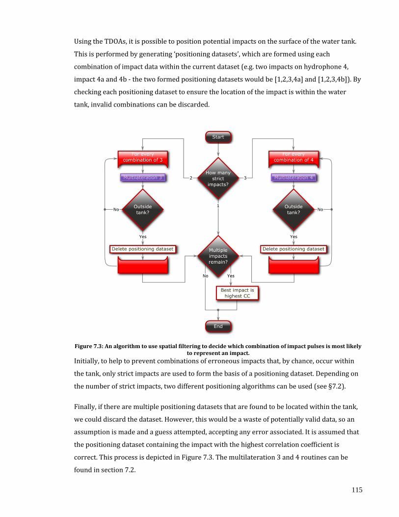
115

Using the TDOAs, it is possible to position potential impacts on the surface of the water tank.

This is performed by generating ‘positioning datasets’, which are formed using each

combination of impact data within the current dataset (e.g. two impacts on hydrophone 4,

impact 4a and 4b - the two formed positioning datasets would be [1,2,3,4a] and [1,2,3,4b]). By

checking each positioning dataset to ensure the location of the impact is within the water

tank, invalid combinations can be discarded.

Figure 7.3: An algorithm to use spatial filtering to decide which combination of impact pulses is most likely

to represent an impact.

Initially, to help to prevent combinations of erroneous impacts that, by chance, occur within

the tank, only strict impacts are used to form the basis of a positioning dataset. Depending on

the number of strict impacts, two different positioning algorithms can be used (see §7.2).

Finally, if there are multiple positioning datasets that are found to be located within the tank,

we could discard the dataset. However, this would be a waste of potentially valid data, so an

assumption is made and a guess attempted, accepting any error associated. It is assumed that

the positioning dataset containing the impact with the highest correlation coefficient is

correct. This process is depicted in Figure 7.3. The multilateration 3 and 4 routines can be

found in section 7.2.

116

7.1.4 Impact decoding wrapper Figure 7.4 illustrates the highest level flow chart specifying the processes applied to the raw

hydrophone data. Colour coded boxes refer to processes that have been specified in sections

7.1.1 to 7.1.3, section 6.3 and section 7.2. The items in black are local to this decision

structure.

Figure 7.4: DSD generation algorithm wrapper.

7.1.4.1 Method

To begin, a supervisory program passes sub-minute raw hydrophone data for processing (a

memory constraint). To remove any mains or wind noise we first band-pass filter at 1-50 kHz

using a 512 order Hamming-window based, linear-phase filter. Next each of the hydrophone’s

raw data is passed to the impact filtering algorithms of Chapter 6. After this has completed, it

117

loops until all the potential impacts have been processed. This starts by generating an impact

dataset (§7.1.1) and checking how many valid impacts are present. If there are less than 3

hydrophones worth of impact data, then the closer inspection of §7.1.2 is performed. If there

are multiple impact data on a single hydrophone the multiple impact analysis of §7.1.3 is

performed. We then use the multilateration wrapper of §7.2 to finalise the position of the

impact.

Similar to §6.2.1.1 a signal to noise (SNR) criterion is used to further check the validity of the

dataset. A mean impact pressure amplitude is divided by the mean RMS noise amplitude and

compared to a threshold (empirically chosen at 2.25). A value greater than this indicates that

it is noise (often a bubble).

Hence, if the dataset is found to originate inside the tank, and the SNR of the impacts is high

enough, then the dataset is considered to be a valid impact and saved. If it is not, then the first

impact is removed, (since the other members of the dataset may belong to a different impact),

and the process is repeated.

At the end of this routine, an array of valid impact locations and amplitudes will be available.

In section 7.4 this data will be converted to an impacting drop size and each drop assigned

into a bin to obtain a DSD.

7.2 Impact positioning – multilateration Using multiple hydrophones solves several problems. If multiple impacts occur at a similar

time, it may be possible to distinguish between them using the algorithms in section 7.1.

Furthermore, the time of arrival (TOA) information for each hydrophone could be used to

predict where the impact landed. After the impact location is known, we can compensate for

any spherical losses and predict a drop size from the normalised amplitude.

7.2.1 Derivation Since there is no notion of an impact start in time, we must use times that are relative to each

other. For a 4 hydrophone setup, it is beneficial to use the difference between each diagonal

pair of hydrophones; this is known as the time difference of arrival (TDOA).

118

Figure 7.5: Depiction of the time difference of arrival (TDOA).

The pressure wave source is the drop impact position on the water surface. This position can

be specified by two parameters in either polar or Cartesian coordinates. If three hydrophones

measure the pressure wave arrival time, two TDOA measurements can be used to calculate

the two-parameter location. However, adding an extra hydrophone increases redundancy,

simplifies the calculations, and ultimately increases the chances of being able to hear a drop.

The process of using the TDOAs to locate a source in 2D space is known as Multilateration.

7.2.1.1 Standard multilateration equations

The process of multilateration may be written as a solution of coupled, multivariate, non-

linear equations. Assuming the impact occurs at time zero and using Pythagoras’ theorem, it is

possible to calculate the TOA from a source at x, y, and z by:

411 222

nzzyyxxc

TOA nnnn (7.1)

where n is the hydrophone number, xn, yn, and zn is the location of the nth hydrophone and c is

the speed of sound in the medium. For this application, z is the known depth of the tank. The

TDOA pairs can be calculated as:

2424

1313

TOATOATDOATOATOATDOA

(7.2)

Expanding:

2

2

2

2

2

2

2

4

2

4

2

424

2

1

2

1

2

1

2

3

2

3

2

313

1

1

zzyyxxzzyyxxc

TDOA

zzyyxxzzyyxxc

TDOA (7.3)

It is now possible to solve (7.3) to find the original position of the source. Equations 7.3

cannot be rearranged to yield closed form solutions for x and y. This is usually rephrased as

an optimisation problem, i.e. find the point (x,y) which minimises the difference between the

measured and predicted TDOAs. Depending upon the algorithms used, the computational

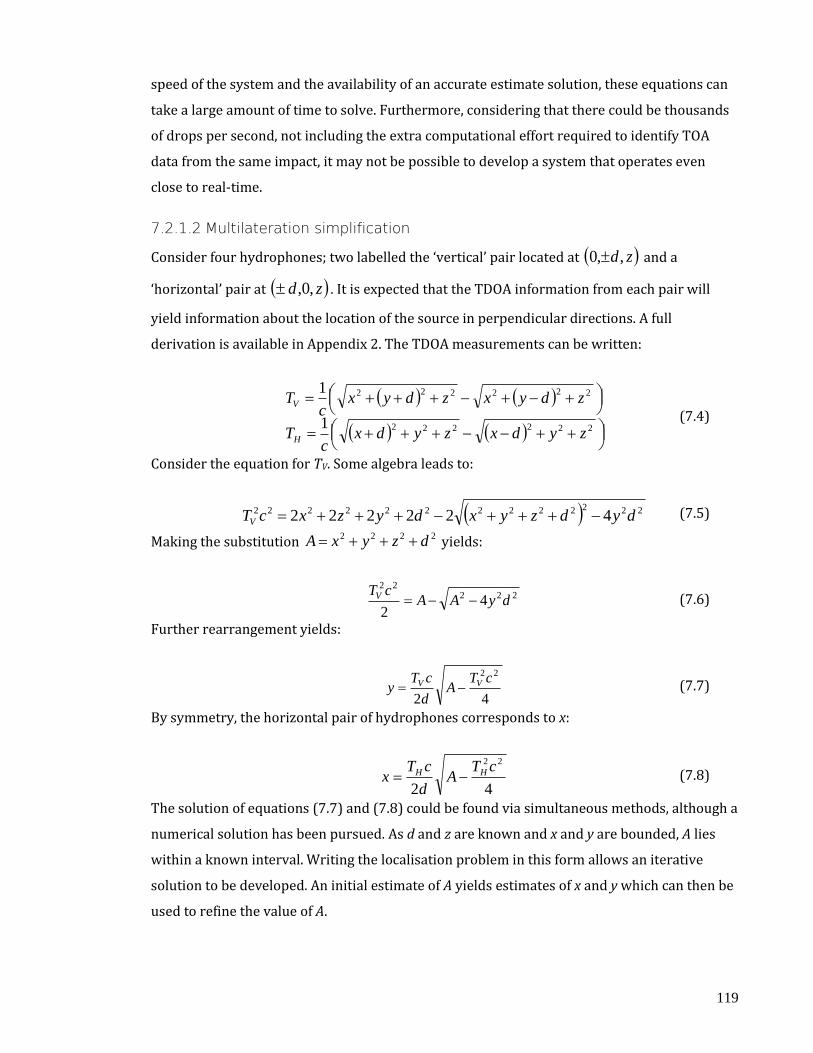
119

speed of the system and the availability of an accurate estimate solution, these equations can

take a large amount of time to solve. Furthermore, considering that there could be thousands

of drops per second, not including the extra computational effort required to identify TOA

data from the same impact, it may not be possible to develop a system that operates even

close to real-time.

7.2.1.2 Multilateration simplification

Consider four hydrophones; two labelled the ‘vertical’ pair located at zd,,0

and a

‘horizontal’ pair at zd ,0, . It is expected that the TDOA information from each pair will

yield information about the location of the source in perpendicular directions. A full

derivation is available in Appendix 2. The TDOA measurements can be written:

222222

222222

1

1

zydxzydxc

T

zdyxzdyxc

T

H

V

(7.4)

Consider the equation for TV. Some algebra leads to:

2222222222222 422222 dydzyxdyzxcTV (7.5)

Making the substitution 2222 dzyxA yields:

22222

42

dyAAcTV (7.6)

Further rearrangement yields:

42

22cTA

d

cTy VV (7.7)

By symmetry, the horizontal pair of hydrophones corresponds to x:

42

22cTA

d

cTx HH (7.8)

The solution of equations (7.7) and (7.8) could be found via simultaneous methods, although a

numerical solution has been pursued. As d and z are known and x and y are bounded, A lies

within a known interval. Writing the localisation problem in this form allows an iterative

solution to be developed. An initial estimate of A yields estimates of x and y which can then be

used to refine the value of A.

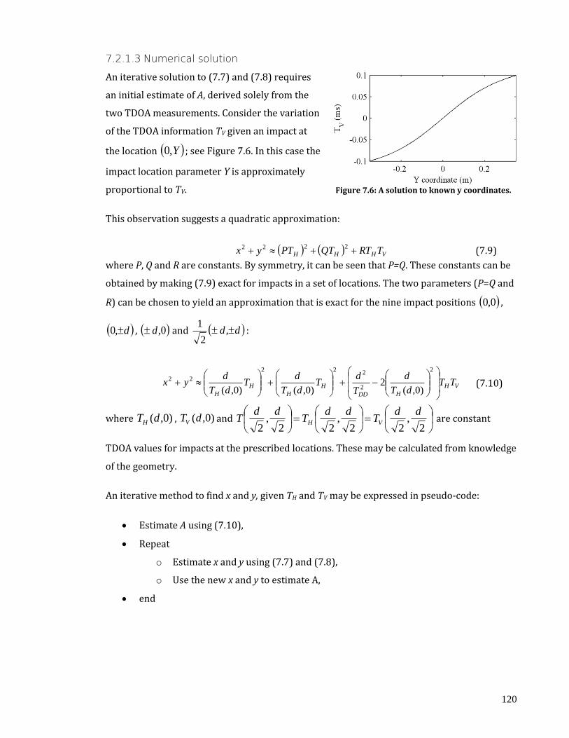
120

7.2.1.3 Numerical solution

An iterative solution to (7.7) and (7.8) requires

an initial estimate of A, derived solely from the

two TDOA measurements. Consider the variation

of the TDOA information TV given an impact at

the location Y,0 ; see Figure 7.6. In this case the

impact location parameter Y is approximately

proportional to TV.

This observation suggests a quadratic approximation:

VHHH TRTQTPTyx 2222 (7.9)

where P, Q and R are constants. By symmetry, it can be seen that P=Q. These constants can be

obtained by making (7.9) exact for impacts in a set of locations. The two parameters (P=Q and

R) can be chosen to yield an approximation that is exact for the nine impact positions 0,0 ,

d,0 , 0,d and dd ,2

1:

VH

HDD

H

H

H

H

TTdT

d

T

dT

dT

dT

dT

dyx

2

2

222

22

)0,(2

)0,()0,( (7.10)

where )0,(dTH , )0,(dTV and

2,

22,

22,

2

ddT

ddT

ddT VH are constant

TDOA values for impacts at the prescribed locations. These may be calculated from knowledge

of the geometry.

An iterative method to find x and y, given TH and TV may be expressed in pseudo-code:

Estimate A using (7.10),

Repeat

o Estimate x and y using (7.7) and (7.8),

o Use the new x and y to estimate A,

end

Figure 7.6: A solution to known y coordinates.

121

After at least 3 iterations of the

simplified multilateration, the

solution can be estimated using

Aitken’s Acceleration. This

extrapolates the results of the

iterations to predict the value the

iterative process is converging to.

Figure 7.7 shows the result of a real

TDOA, (generation of the TDOA from

real x, y, coordinates), and the solved

TDOA (calculating x, y, coordinates from the TDOA’s). After the Aitken’s Acceleration the

result is highly accurate and computationally efficient. As a comparison, with this algorithm 1

second’s worth of 100mm h-1 rain data now takes 140 seconds; an improvement that is 128

times faster than the best previous method. Note that this is not a final computational time,

since this time was based upon a simulated DSD. Since we will not be able to hear the majority

of the smaller drops, this time will decrease dramatically, to a point where it is negligible

when compared to other processing tasks (e.g. raw signal filtering).

7.2.2 Testing To test the multilateration routines, a 0.5 m2 circular tank was lined with the anechoic of

section 3.3 to yield an effective radius of 0.35m (area = 0.38 m2). A syringe with a hypodermic

needle was positioned near the centre of the tank using a clamp and stand approximately 1 m

above the waterline. The impact position of the drops were then measured, although

depending on the wind and how a droplet dislodges from the needle head, the spread of the

droplets could be up to ±5cm. Figure 7.8 shows the results from such a test. It is possible to

see a spread of the droplets and that they are not centred around the (0, 0) point. This is likely

due to an initial measurement error and a slight wind. Figure 7.9 is a zoomed version of the

Figure 10. It shows the effect of position quantisation, which is defined by the sampling rate of

the data acquisition card. This could be mitigated by performing spline interpolation before

the impact filtering routines take place, however this would increase the computational effort

required.

Figure 7.7: A solution to the multilateration routines using

iteration and Aitken’s acceleration.

122

Figure 7.8: Testing the multilateration routines. Crosses are solutions to a dataset, stars are the locations of hydrophones and the line is the tank boundary.

Figure 7.9: A zoomed-in version of Figure 7.8.

7.2.3 Three- and four-hydrophone multilateration algorithms The multilateration algorithms are developed in section 7.2.1. The two different versions,

three- and four-hydrophones, are largely identical.

7.2.3.1 Three hydrophone multilateration

A three-hydrophone version of the multilateration algorithms is possible due to the depth of

the tank being fixed. Impact pressure wave arrival times at three hydrophones provide two

TDOA measurements and these uniquely determine the two impact location parameters.

However, the simplification and algorithms developed in section 7.2.1.2 are not directly

applicable. Instead, the TDOA corresponding to the pair with an unknown TOA is set to zero

(i.e. the centre of the tank). The iteration of section 7.2.1.3 is then used by updating the

prediction of the unknown TOA until convergence. The inaccuracy of the initial estimation will

increase the number of iterations required for convergence and therefore increase the

computational requirement.

7.2.3.2 Method

The four-hydrophone version begins by calculating the TODAs and forming an initial location

estimate based upon (7.10). Three levels of iteration then begin, recalculating the location and

TODAs each time. Finally Aitkin’s acceleration is used to find the point of convergence and a

final impact location.

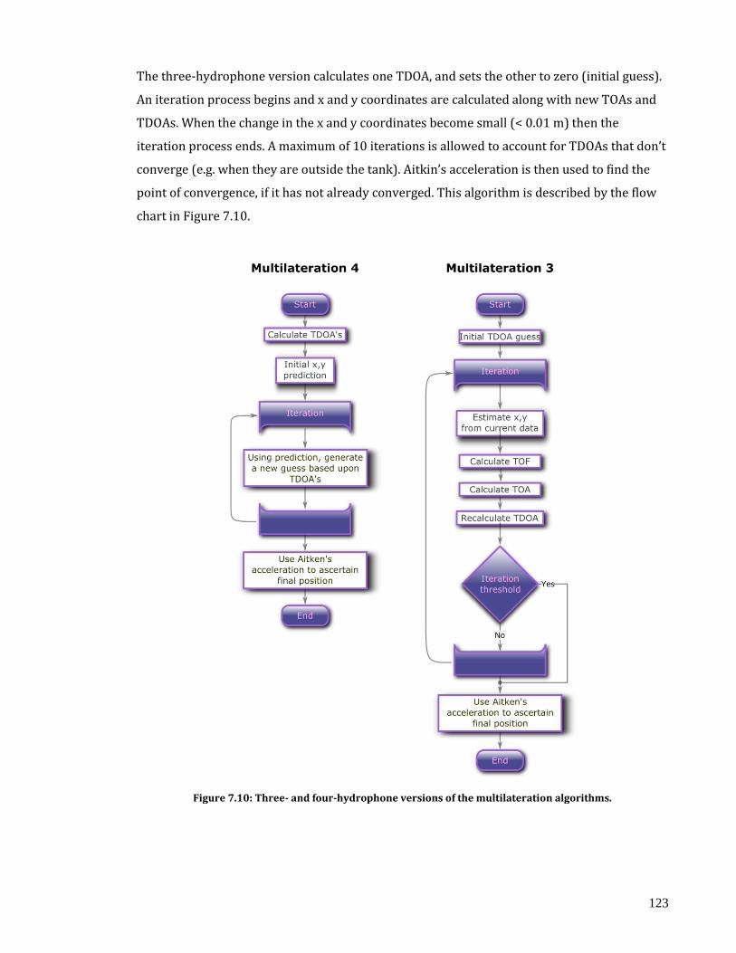
123

The three-hydrophone version calculates one TDOA, and sets the other to zero (initial guess).

An iteration process begins and x and y coordinates are calculated along with new TOAs and

TDOAs. When the change in the x and y coordinates become small (< 0.01 m) then the

iteration process ends. A maximum of 10 iterations is allowed to account for TDOAs that don’t

converge (e.g. when they are outside the tank). Aitkin’s acceleration is then used to find the

point of convergence, if it has not already converged. This algorithm is described by the flow

chart in Figure 7.10.

Figure 7.10: Three- and four-hydrophone versions of the multilateration algorithms.

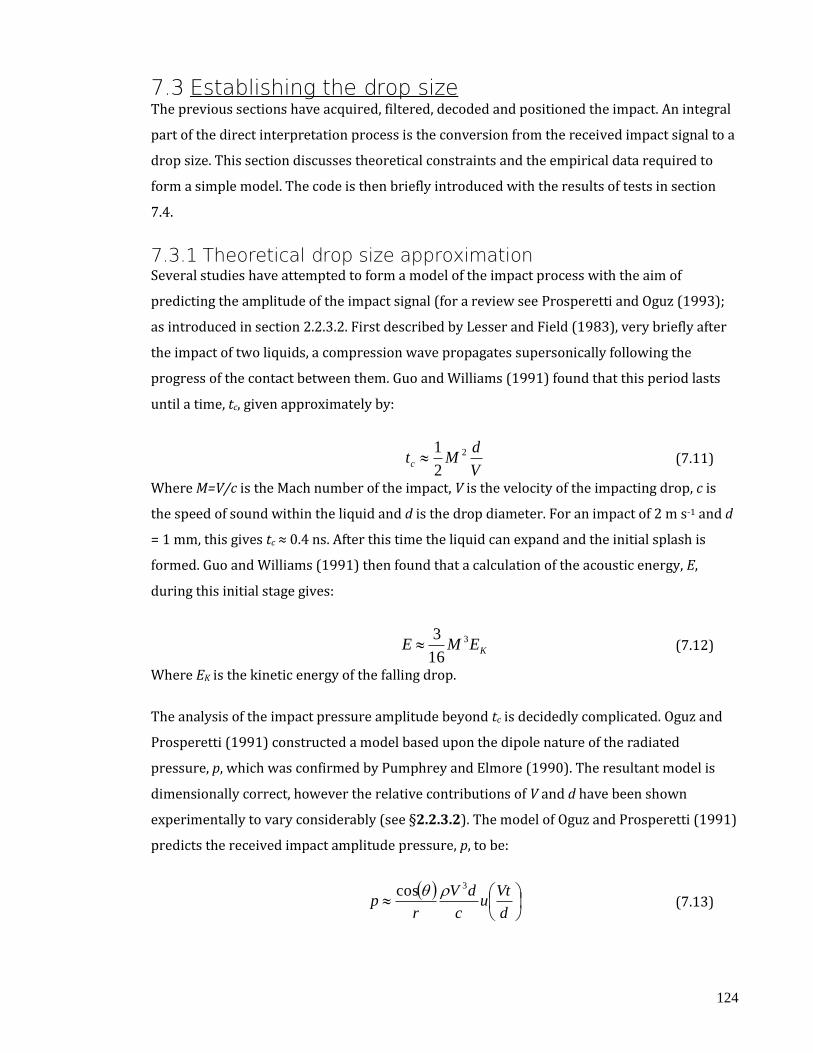
124

7.3 Establishing the drop size The previous sections have acquired, filtered, decoded and positioned the impact. An integral

part of the direct interpretation process is the conversion from the received impact signal to a

drop size. This section discusses theoretical constraints and the empirical data required to

form a simple model. The code is then briefly introduced with the results of tests in section

7.4.

7.3.1 Theoretical drop size approximation Several studies have attempted to form a model of the impact process with the aim of

predicting the amplitude of the impact signal (for a review see Prosperetti and Oguz (1993);

as introduced in section 2.2.3.2. First described by Lesser and Field (1983), very briefly after

the impact of two liquids, a compression wave propagates supersonically following the

progress of the contact between them. Guo and Williams (1991) found that this period lasts

until a time, tc, given approximately by:

V

dMtc

2

2

1 (7.11)

Where M=V/c is the Mach number of the impact, V is the velocity of the impacting drop, c is

the speed of sound within the liquid and d is the drop diameter. For an impact of 2 m s-1 and d

= 1 mm, this gives tc ≈ 0.4 ns. After this time the liquid can expand and the initial splash is

formed. Guo and Williams (1991) then found that a calculation of the acoustic energy, E,

during this initial stage gives:

KEME 3

16

3 (7.12)

Where EK is the kinetic energy of the falling drop.

The analysis of the impact pressure amplitude beyond tc is decidedly complicated. Oguz and

Prosperetti (1991) constructed a model based upon the dipole nature of the radiated

pressure, p, which was confirmed by Pumphrey and Elmore (1990). The resultant model is

dimensionally correct, however the relative contributions of V and d have been shown

experimentally to vary considerably (see §2.2.3.2). The model of Oguz and Prosperetti (1991)

predicts the received impact amplitude pressure, p, to be:

d

Vtu

c

dV

rp

3cos (7.13)

125

Where θ and r are the azimuth angle and distance from the water plane to the listening device,

ρ is the density of the water and u is a dimensionless function that describes the ‘details of the

process’ - Prosperetti and Oguz (1993).

7.3.2 Experimental drop size approximation Models of the impact wave produced by a water drop impacting on a water surface agree that

a dipole-like wave will be produced and that the pressure will decrease with the reciprocal of

range. Beyond this, the link between drop parameters and the amplitude of the impact wave

are less well known. Although a range of complex empirical expressions exist, (e.g. those of

Pumphrey et al. (1989), Pumphrey (1991)), calibration would be necessary using the

geometry, material and equipment of the AWTD.

7.3.2.1 Drop velocity testing

Although not directly relevant to the final pressure-to-drop size model, it is interesting to note

the differences measured by our equipment when compared to the referenced results. Using

the available equipment it is possible to observe how the velocity of a drop alters the resultant

impact pressure. Furthermore, it is possible to design an experiment to provide a model to

convert the received impact pressure amplitude into a drop size.

7.3.2.1.1 Experimental procedure The aim is to create consistently sized drops at differing impact velocities. Using a gravity fed

syringe connected to a suitably sized hypodermic needle reasonably consistent rain drops, of

a size that is dependent on the diameter of the needle, could be produced. The drops will then

accelerate due to gravity and may reach their terminal velocity before they impact on the

water’s surface.

By placing the LPM as close to the surface of the water as possible (so not to accelerate further

between the LPM catchment area and the water’s surface) the drop velocity and size can be

measured. The velocity can then be compared to the pressure received by the AWTD.

126

7.3.2.1.2 Results Drops of diameter 3.54 ±0.17 mm

were allowed to fall through the LPM

catchment area from heights

between 0.5 and 2.5 m. After

averaging the velocity for each

height, Figure 7.11 shows the results

and power-law regression. It was

difficult to link individual drops to

pressure measurements due to

variable delays within the LPM and

in the communications between the

LPM and computer. This forced the use of averaged velocity readings taken from the LPM and

causes the apparent velocity quantisation in Figure 7.11.

The least-squares power-law fit suggests that the impact pressure is proportional to the

velocity to a power of 2.9. This is consistent with the results of Pumphrey et al. (1989) and

Pumphrey (1991) who suggest that it is proportional to a power of between 2.5 and 3, and

2.8±0.2, respectively.

7.3.2.2 Impact pressure testing

The method and results of the pressure-to-drop size calibration exercise are presented here.

The measured amplitude of the pressure wave depends upon the size and fall-speed of the

rain drops. These will be used in the main DSD generation routines of the direct interpretation

method to correctly qualify the size of the impacting drop. An incorrect calibration will cause

the data to be skewed along the drop size axis.

7.3.2.2.1 Experimental procedure Similar to the experiment of 7.3.2.1, the aim of this experiment is to match the LPM size data

to the pressure amplitude of the impact wave derived from the AWTD hydrophone data. A lid

was placed over the AWTD with an aperture immediately below the LPM catchment and

directly above one of the hydrophones. This fixes the distance travelled by a propagating

impact wave to the depth of the tank (0.59 m) and only allows raindrops into the tank that

have passed through the LPM catchment first.

A rain event was then artificially simulated using an elevated sprinkler. The resultant drops

travelled a total vertical drop of approximately 8 m; hence, the majority of small to medium

Figure 7.11: Plotting the impact velocity vs. pressure. Points are individual impacts from heights between 0.5 and 2.5m. The line is the least-squares best fit which shows that the

pressure is proportional to the velocity to a power of 2.86, which is in agreement with published results.

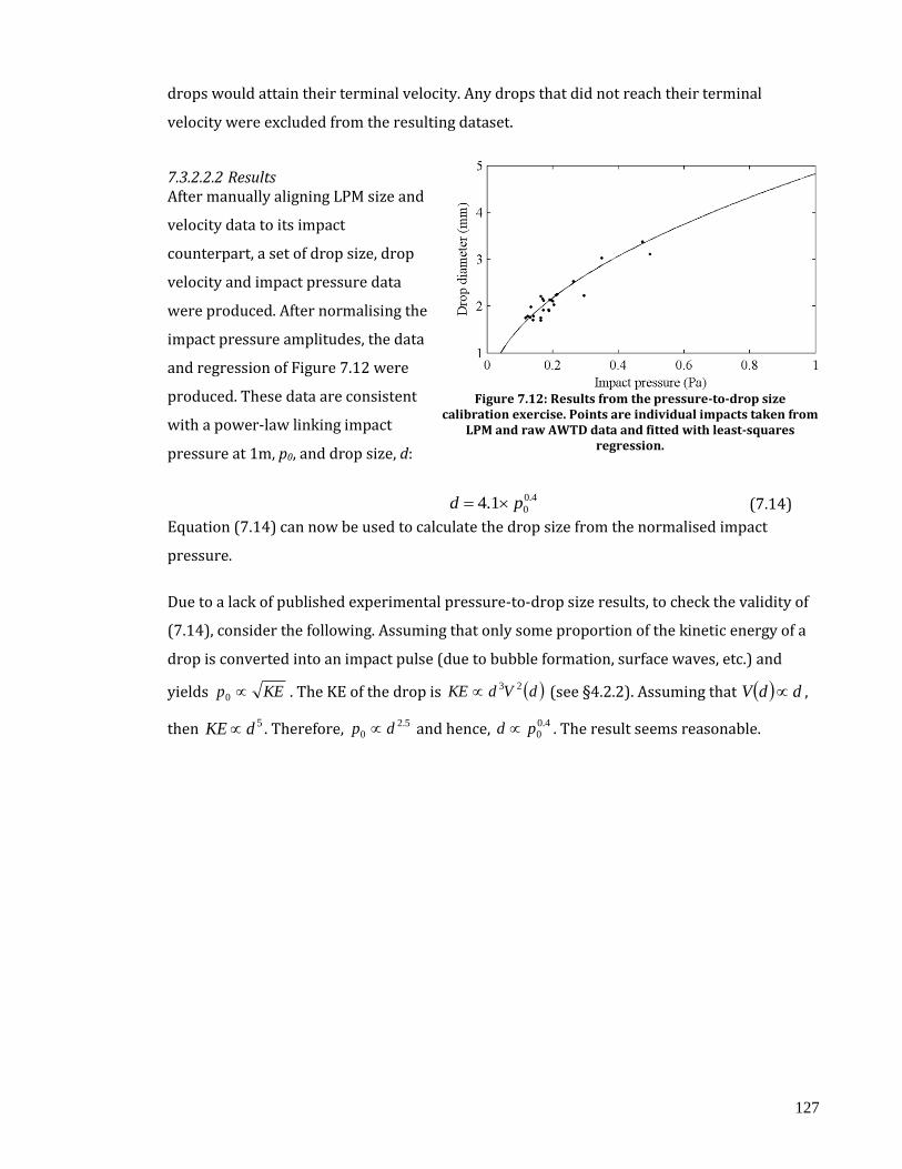
127

drops would attain their terminal velocity. Any drops that did not reach their terminal

velocity were excluded from the resulting dataset.

7.3.2.2.2 Results After manually aligning LPM size and

velocity data to its impact

counterpart, a set of drop size, drop

velocity and impact pressure data

were produced. After normalising the

impact pressure amplitudes, the data

and regression of Figure 7.12 were

produced. These data are consistent

with a power-law linking impact

pressure at 1m, p0, and drop size, d:

4.0

01.4 pd (7.14)

Equation (7.14) can now be used to calculate the drop size from the normalised impact

pressure.

Due to a lack of published experimental pressure-to-drop size results, to check the validity of

(7.14), consider the following. Assuming that only some proportion of the kinetic energy of a

drop is converted into an impact pulse (due to bubble formation, surface waves, etc.) and

yields KEp 0 . The KE of the drop is dVdKE 23 (see §4.2.2). Assuming that ddV ,

then 5dKE . Therefore, 5.20 dp and hence, 4.0

0pd . The result seems reasonable.

Figure 7.12: Results from the pressure-to-drop size

calibration exercise. Points are individual impacts taken from LPM and raw AWTD data and fitted with least-squares

regression.

128

7.3.3 Application of drop size approximations With a working impact pressure-to-drop size model, the final

section of the code is presented in Figure 7.13. Here, each validated

dataset (i.e. inside the tank and a high SNR) is converted into a drop

size. The drop impact position is calculated by multilateration and

then the distance and azimuth angle to each hydrophone is

calculated. This information is used to calculate the normalised

pressure which is then calibrated using a multiplier obtained from

the calibration experiment (see Appendix 1). Equation (7.14) is

then used to calculate the drop diameter. The final diameter

estimate is the average of the diameters calculated from each of the

four hydrophones. Finally the drop diameter is saved into a DSD for

later analysis (see §7.4).

7.4 DSD generation The algorithms of the previous sections can be used to generate and

analyse DSD results. A comparison will be made between the DSD of

the LPM and the DSD generated by the AWTD. The measure of

success will be how similar the two distributions are. Initially the

results are presented with an explanation of observations and

inherent errors are discussed later (§7.4.2)

7.4.1 DSD results and comparison A total of 26.6 hours of rain data collected over a period of 6 months, have been converted

into minute long DSD distributions. The data collection period overlapped with the driest six

months in the UK for 80 years. Figure 7.14 plots the average LPM DSD data against the

average AWTD generated DSD data. Error bars (shading), representing the average standard

error for each bin, are also plotted. It can be seen that the AWTD DSD approximates the LPM

DSD very well (a quantitative analysis will be presented later - §7.4.1.3).

Figure 7.13: Drop

normalisation and sizing routine.

129

Figure 7.14: The averaged DSDs from the LPM (black) and the AWTD (red) with associated standard errors for

each bin (shading).

7.4.1.1 Individual DSD examples

The benefits of the AWTD’s large catchment area can be seen in the large drop tail in the

derived DSD. Here the data is either highly uncertain or non-existent for the LPM, while the

AWTD has measured sizable numbers of drops. A major feature of the AWTD is that the much

larger catchment area provides much better estimates of the numbers of large drops.

Alternatively, DSD can be estimated with the same accuracy as with the LPM but for

integration times a factor of 85 times shorter.

Several examples of the individual 1 min DSDs can be seen in Figure 7.15. One can visually

apply a gamma distribution fit to find that even in the most extreme circumstances, (i.e. the

LPM does not see any large drops: e.g. the DSDs in the east and south-west positions), the

results are largely agreeable.

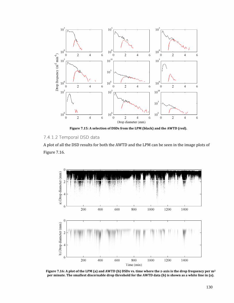
130

Figure 7.15: A selection of DSDs from the LPM (black) and the AWTD (red).

7.4.1.2 Temporal DSD data

A plot of all the DSD results for both the AWTD and the LPM can be seen in the image plots of

Figure 7.16.

Figure 7.16: A plot of the LPM (a) and AWTD (b) DSDs vs. time where the z-axis is the drop frequency per m2 per minute. The smallest discernable drop threshold for the AWTD data (b) is shown as a white line in (a).

131

In Figure 7.16, the plot of the LPM’s DSD, (a), compared to the AWTD’s DSD, (b), is not detailed

enough to be able to accurately represent the large drop tail of the DSD. This manifests in this

image by making the data look pixelated. For example, consider the event at approximately

505 minutes. The LPM data describes the event as a fairly long (wide) event with a maximum

drop size of approximately 3 mm. However, the AWTD shows that for a brief time within the

event the maximum drop size increases dramatically to above 5 mm. This type of event could

very easily prevent a communications link from operating and the LPM does not show this.

One discrepancy that severely degrades the temporal correlation (§7.4.1.3) is the event-long

error between 1065 and 1085 minutes in Figure 7.16. The cause of this error is unknown and

is open to speculation. It could be that bubbles were masking impacts or due to non-liquid

hydrometeors. It could even be due to non-meteorological effects such as insects or animals

(e.g. spiders spinning a web around the lens of the LPM) or simply, an error within either

instrument.

7.4.1.3 Time series analysis

The lack of comparative data makes a quantitative analysis difficult. One method of

comparison is to fit an exponential (M-P) distribution to each minute long DSD. This yields

scale and shape parameters that can be compared over time to provide a temporal correlation

coefficient. Section 2.1.2.3 found that a gamma distribution better described the atmospheric

DSD over short timescales. Using an exponential distribution on DSDs that hasn’t been

averaged will result in erroneous fits. However, for the purposes of comparison, the increased

error is less important than the simplicity of single shape and scale parameters.

Figures 7.17 and 7.18 depict the shape (μ) and scale parameters of a maximum likelihood-

fitted exponential distribution to each minute long DSD. Figure 7.17 shows the shape

parameter for all drop diameters. A scale parameter for all drop diameters is not plotted since

it is a function of the number of observations, which is disproportionately underestimated by

the AWTD (it cannot hear drops below 1.8 mm and potentially misses thousands of drops).

However, it can be seen that the AWTD fits the LPMs shape parameter well and results in a

Pearson correlation coefficient of 0.70.

The scale parameter for drops above diameters of 1.8 mm is shown in Figure 7.18. Above 1.8

mm, the AWTD should be recording the same number of observations as the LPM. Therefore,

the scale parameter of the exponential fits can be compared. The shape parameter is not

plotted since a fit could not be justified considering the lack of large drop size LPM data. The

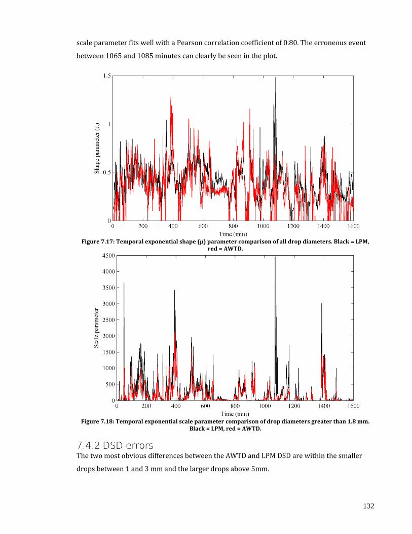
132

scale parameter fits well with a Pearson correlation coefficient of 0.80. The erroneous event

between 1065 and 1085 minutes can clearly be seen in the plot.

Figure 7.17: Temporal exponential shape (μ) parameter comparison of all drop diameters. Black = LPM,

red = AWTD.

Figure 7.18: Temporal exponential scale parameter comparison of drop diameters greater than 1.8 mm.

Black = LPM, red = AWTD.

7.4.2 DSD errors The two most obvious differences between the AWTD and LPM DSD are within the smaller

drops between 1 and 3 mm and the larger drops above 5mm.

133

Below a diameter of approximately 2.5 mm the drop impacts become increasingly difficult to

distinguish from noise and drops are missed. This happens over a range of drop sizes due to

the location of the impacting drop. Consider a drop impacting at the centre of the tank. All

hydrophones should be able to hear the impact at approximately similar amplitudes. If the

impact filtering routines can detect one impact, it should be able to detect them all. If a small

drop impacts at an extremity of the tank, it is likely that one hydrophone should be able to

hear the impact well, whereas the opposite hydrophone may not be able to hear the impact at

all. If the impact decoding routines cannot compensate for this error, the dataset is discarded

and the information about the impact is lost. Above diameters of approximately 3 mm all

hydrophones can hear an impact, irrespective of where the impact occurs in the tank.

However, for the purposes of DSD generation, the smallest discernable drop is taken at the

point where the AWTD DSD begins to tend towards the LPM DSD; at 1.8 mm.

Above 5 mm, the AWTD appears to measure more large drops than the LPM DSD. The

atmospheric sampling statistics are very poor for these drop bins (see §. The LPM has

measured a total of only a few tens of these drops and so large variation between LPM and

AWTD numbers is expected. However, there is probably a systematic error in either or both of

the devices leading to DSD divergence at this large drop diameters.Inherent AWTD errors

There are many mechanisms that could reduce the accuracy of the AWTD DSD. Looking at

each possible static (i.e. always possible) error in turn:

Changes of tank depth due to evaporation.

Errors in the calibration equation (7.14).

Changes in the speed of sound in the tank due to temperature and contaminants.

Organic growth could be absorbing/reflecting some of the sound energy.

An increased impact velocity due to wind. This is recorded on the AWTD as a greater

impact pressure and hence, a greater impact size (see §4.3.5).

For example, the temperature dependence on the speed of sound could be a large source of

error. At 5 °C, the speed of sound is equal to 1425 m s-1, whereas at 20 °C it is 1480 m s-1. This

could cause a conversion error in the multilateration algorithms. At a depth of 0.59 m, the

differences in speeds cause a TOA error of 15 μs, or 3 samples of the DAQ. At 10 °C this is a

distance error of 2.5cm. This error would propagate through the software to yield an

inaccurate drop size.

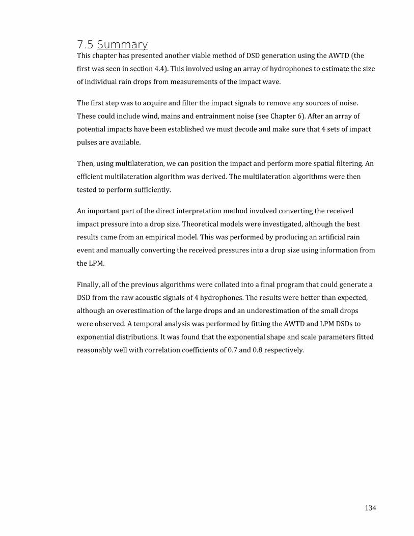
134

7.5 Summary This chapter has presented another viable method of DSD generation using the AWTD (the

first was seen in section 4.4). This involved using an array of hydrophones to estimate the size

of individual rain drops from measurements of the impact wave.

The first step was to acquire and filter the impact signals to remove any sources of noise.

These could include wind, mains and entrainment noise (see Chapter 6). After an array of

potential impacts have been established we must decode and make sure that 4 sets of impact

pulses are available.

Then, using multilateration, we can position the impact and perform more spatial filtering. An

efficient multilateration algorithm was derived. The multilateration algorithms were then

tested to perform sufficiently.

An important part of the direct interpretation method involved converting the received

impact pressure into a drop size. Theoretical models were investigated, although the best

results came from an empirical model. This was performed by producing an artificial rain

event and manually converting the received pressures into a drop size using information from

the LPM.

Finally, all of the previous algorithms were collated into a final program that could generate a

DSD from the raw acoustic signals of 4 hydrophones. The results were better than expected,

although an overestimation of the large drops and an underestimation of the small drops

were observed. A temporal analysis was performed by fitting the AWTD and LPM DSDs to

exponential distributions. It was found that the exponential shape and scale parameters fitted

reasonably well with correlation coefficients of 0.7 and 0.8 respectively.

135

Chapter 8: Summary and conclusions

In this final chapter, the work which has been detailed in the previous sections is concluded

and summarised, followed by recommendations for future work.

8.1 Final summary An understanding of the hydrological cycle is important when approaching a meteorological

project. Chapter 2 presented an introduction, detailing the processes and mechanisms that

define rainfall. Water vapour and droplets undergo a turbulent process in which they grow to

a size until they begin to fall back towards the Earth. A drop can increase in size due to

coalescence and condensation; where it collides with other water droplets or it absorbs water

vapour from the atmosphere. Raindrops typically impact the ground with sizes between 0.5

and 6 mm. Smaller drops are generally considered to be drizzle or fog while larger drops are

very rare and no drops larger than 10 mm have been measured.

The rain drop size distribution (DSD) contains a lot of information about the rain and many

application parameters can be derived from it. For large sample volumes, the DSD can be

approximated by a two-parameter exponential, or Marshall-Palmer distribution. However, for

small integration volumes it is often more accurate to use a three parameter Gamma

136

distribution. The parameters of this distribution are all independent and important in other

areas of meteorology (e.g. radar).

An impacting drop upon a pool of water creates several distinct sounds. It was proposed that

these sounds could be investigated and used to provide an estimation of the DSD across the

pool’s surface. The impact sound typically has two constituents: a sound corresponding to the

initial impact and the sound that is generated by oscillating bubbles trapped under the

surface. The process of bubble production is known as entrainment. Entrainment contains

little information, since it does not occur all of the time and it only occurs for specific drop

sizes. The impact sound however, is of interest, as the received pressure is proportional to

some power of the drop size and drop velocity. Assuming a terminal drop velocity, the drop

size could be estimated from the impact sound.

A discussion of other disdrometers was presented, identifying limitations with commercial

instruments. The greatest advantage of the AWTD is the increased catchment area. Large

drops are of significant interest to radio scientists and geomorphologists since they cause the

most attenuation in communication links and the largest amount of soil detachment.

However, large drops do not occur very often and consequently their number density is

poorly estimated by disdrometers with small catchment areas. This results in a large variance

in the large-drop tail of DSDs measured using commercial instruments.

Other authors have attempted to use the same acoustic signal in the past, although much of

the work has been performed using the total acoustic sound field and at sea. One author had

attempted to interpret individual drops, but was unable to provide DSD results. The use of a

water tank decreased the amount of background noise and enabled the instrument to be used

on land.

Chapter 3 described a complete design and implementation of the AWTD and outlined the

importance of component selection. An emphasis was placed on low noise electronics to

improve the chances of being able to hear small drops. Hydrophone placement also became an

important feature, due to the dipole-like nature of the impact sound. An effort to correctly

match all impedances between the hydrophone and the DAQ was made which yielded a highly

sensitive acoustic system.

Also, an anechoic lining was developed to reduce the chances of the system incorrectly

considering a reflection as an impact. An experimental process included testing a selection of

137

materials. It was found that a combination of natural rubber backed with a light foam

performed well for a very low cost.

Chapter 4 dealt with the formulation of algorithms to infer kinetic energy flux densities and

rain intensities from the total sound field. Comparison of estimated parameters with those

measured by a commercial laser precipitation monitor (LPM) required estimates of

uncertainties due to differing sample volumes. The errors associated with the atmospheric

sampling of the LPM and the AWTD were investigated theoretically and it was demonstrated

that the parameter variance was inversely proportional to the product of catchment area and

integration time. Therefore, the AWTD can produce results with the same variance at an

integration time 85 times smaller than the LPM. The AWTD can produce parameter estimates

with an integration time of 0.7 s with the same sampling uncertainty as the LPM using a one-

minute the AWTD integration time could be reduced.

It was proposed that all of the kinetic energy of a drop would be converted into acoustical

energy (neglecting splashes outside the tank, drops hitting the sides, etc.). By listening to the

total acoustic sound field a simple linear relationship between the raw data and the KE flux

density could be established. This was verified in section 5.4 by collecting 6 months worth of

rainfall data. Comparing the AWTD data to KE flux density records showed a very high

Pearson correlation coefficient of 0.92. This compares well to comparisons of co-sited

commercial disdrometer reported by other authors. The AWTD data could also be inverted to

RI data using a similar method. Results yielded Pearson correlation coefficients of 0.81,

yielding a broad agreement to the LPM and compares well to the results of other authors.

Increasing the temporal resolution of the AWTD yielded interesting temporal structure

highlighting the large variation of both the KE flux density and the RI. In the example

provided, the LPM reported a maximum RI of approximately 12 mm h-1. However, the AWTD

yielded 1 second resolution RIs greater than 70 mm h-1 . This fine-structure RI variation is

likely to be critical in the design of short (a few tens of metres) communications links

operating in the higher microwave frequency bands. Such links operating around 80 GHz are

currently being deployed.

The effect of wind on the AWTD data was briefly investigated and it was found that in high

wind events the discrepancies between LPM and AWTD measured parameters increase

dramatically. This is due to the LPM limitation of only measuring the vertical component of

the drop velocity. This makes the AWTD generated KE measurements potentially more

138

accurate in high wind events as an increase in drop kinetic energy will increase the resultant

acoustic energy.

It was found to be possible to estimate the three parameters of a Gamma distribution using

the AWTD total sound field data. Averaging all the DSD data over 6-months yields a Pearson

correlation coefficient of 0.9 with the similar distribution measured using the LPM. However,

the short time (1 minute) DSD showed more variation with correlation coefficients of 0.69

being common.

Chapter 5 investigated the problems caused by entrainment. It was established that

entrainment noise would cause the majority of the error within the AWTD results unless steps

could be taken to mitigate their occurrence, or their effect. Several methods were investigated.

Using a surfactant to change the properties of the liquid was considered. It was found that use

of an oil film to cushion the impact and thus prevent crater formation and collapse, eliminated

bubble production. However, various impracticalities, including high maintenance

requirements, prevented the use of oil films in the AWTD.

It was thought that it may be possible to force the bubbles to oscillate in a controllable way.

By generating a high powered, sinusoidal, acoustic filed in the water surrounding bubble, it

was hoped that the bubble would resonate at the same frequency as the forcing signal. Simple

software filtering could then be used to remove all traces of the bubble noise. However,

experimentation and simulations based on a theoretical model showed that this would not be

possible.

Chapter 6 investigated a signal processing method of impact detection; to attempt to identify

and remove entrainment signals from the data. It first considered other sources of noise and

investigated the properties of impact and bubble signals. It was found that simple frequency

discrimination would not be possible.

Three different filtering methods have been investigated: matched (correlation), power

(Hilbert) and wavelet. It was found that the wavelet method was the most successful with a

30% underestimation of the true impact population. The Hilbert method performed the worst

due to errors caused by bubble oscillations just crossing a threshold. The correlation method

worked fairly well, although it was highly susceptible to noise.

139

The wavelet method was used in the final direct interpretation routines to generate a DSD. It

is expected that the error introduced by the wavelet filtering will be reduced by the advanced

spatial filtering methods also incorporated in the AWTD system.

Chapter 7 described the ultimate progression of the AWTD. By using an array of hydrophones

in the tank it is possible to pick out each individual drop and convert the received pressure to

a drop size. This chapter details the methodology and algorithms of the entire process from

capture to dissemination. The steps in the data processing sequence can be summarised:

1. Filtering of hydrophone signals to remove noise,

2. Identification of impact signals,

3. Identification of impact signals from different hydrophones generated by the same

drop,

4. Localisation of drop impact position,

5. Estimation of drop size,

6. Collection of drop size information into DSD.

The final averaged DSD results show a strong similarity between the LPM and AWTD. In

general, the AWTD measured more large drops and fewer small drops than the LPM. A

smallest discernable drop diameter of 1.8 mm is clearly visible. The lack of data below 1.8 mm

makes the direct use of a correlation coefficient to describe the accuracy unsuitable.

To facilitate a comparison, temporal analysis was performed by fitting an exponential

distribution to both LPM and AWTD derived DSDs with a one-minute integration time. The

resultant shape and scale parameters were compared to find that they fitted reasonably well

with correlation coefficients of 0.7 and 0.8 respectively.

8.2 Further work The most obvious route for further work is to commercialise the AWTD and formalise its

software. However, throughout the trials of the instrument it was found that using a water

tank, which is its main benefit, is also its downfall.

The greatest problem with the AWTD is its inherent lack of robustness. Other commercial

disdrometers can be left in the field for years of continuous usage. After a period of a few

months organic growth began to take hold within the tank. In the winter it froze and in the

summer the water evaporated. Furthermore, on several different occasions the hydrophones

140

failed. These problems could be fixed in a number of different ways, but also point to a

different, but similar product.

8.2.1 Further additions to the AWTD We have already talked about several additions that would be beneficial to the AWTD.

Freezing of the water in the tank made the AWTD unavailable for much of the winter.

Furthermore, the speed of sound in the tank is a function of water temperature and this leads

to uncertainty in drop size estimation. A temperature sensor in the tank would allow for

automatic detection of freezing and accurate estimation of acoustic phase velocity.

Alternatively, the tank could be heated and maintained at a constant operational temperature.

The depth of the tank also effects drop size estimation. Over summer evaporation caused the

tank level to drop by up to 8 cm. Automation of the tank depth measurement would be

beneficial, as this parameter could be used in drop size estimation. Alternatively, the tank

level could be easily maintained automatically by a float valve outside the catchment area.

If the AWTD was to be used purely to generate KE flux density or RI results, the system would

only require a single hydrophone and no anechoic lining. This would significantly reduce the

cost of the system.

The 24-bit DAQ is not necessary for such a system. Costs could be saved by replacing the DAQ

with a more affordable model. A DAQ with an increased sampling rate would reduce the

quantisation effects of §7.2.2.

A wind sensor was used to examine the error introduced into the KE flux density

measurements using the LPM due to horizontal movement of the drops. If KE flux density is

the desired parameter then the AWTD provides this. However, if the AWTD is used for RI

estimation then a wind sensor would be necessary for wind speeds above an average of 2.5 m

s-1.

8.2.2 The use of a digital signal processor By converting all of the software developed and used on a standard PC to a form that could be

placed within a common digital signal processor (DSP), the cost of such an instrument would

be significantly reduced (by approximately the cost of a powerful PC). Another option would

be to use a dedicated ‘miniature’ PC which holds all the same components, but in a smaller

size. This would be beneficial as the AWTD could be manufactured as a single unit to improve

robustness and reduce power consumption.

141

8.2.3 The acoustic metal plate disdrometer The use of water as a catchment material has both advantages and disadvantages. The major

advantages are the rapid and consistent transformation of drop kinetic energy to acoustic

energy, and the low loss transmission of acoustic energy from drop impact to hydrophone.

Many of the disadvantages have been discussed previously. If an instrument is to be used only

for KE measurement, and possibly RI estimation, then the complexities of the AWTD are

unnecessary. A catchment is necessary with the following properties:

1. Efficient and consistent transformation of energy;

2. Low loss transmission of acoustic energy to measurement device;

3. Short reverberation time.

An engineered metal plate could satisfy these constraints. Losses in energy transformation

would be due to acoustic energy propagating in air and consistency would be affected by

splash processes. A standard microphone could be used to detect acoustic energy in the plate.

Acoustic energy would be strongly reflected at the metal-air interfaces and this could lead to

long reverberation times. Reflection from the edges could be reduced by shaping the edges

into points. Fundamental modes of oscillation could be mechanically damped. The metal plate

could be heated in cool temperatures to mitigate the cushioning effect of snow. A dedicated

digital DSP could be used to compute the information. By effectively mounting and protecting

the microphones and processor from the elements, this would result in a completely closed,

robust product. Using microphones and a common DSP would significantly decrease the cost

of such a system.

8.2.4 The acoustic tent disdrometer Similar to §8.2.3, another option would be to use a tent-like structure above several

microphones. The AWTD algorithms could be transferred to such a device with little

alteration. However, considerable effort would be required to control the performance of the

tent in converting drop KE to measured acoustic energy. Some of the incident drop KE would

be absorbed by bulk oscillations of the tent structure and these may reverberate for more

than a second. It would be difficult to make the tent spatially uniform in its energy transfer

efficiency. Also the tent structure is likely to radiate sound in preferred directions and these

would need to be understood and utilised.

142

8.3 Concluding remarks This project has produced a demonstration disdrometer that can measure rain kinetic energy

flux density, rain intensity and DSD with a much greater temporal resolution when compared

the LPM (as a direct comparison). Extending the catchment area argument to other

disdrometers implies that the AWTD performs better than any other commercial alternative

(e.g. impact disdrometer, 2D video disdrometer). It can produce rain intensity and kinetic

energy flux density information at integration times as low as 1 second. Results have shown

that there are large scale variations in these parameters that are not seen with instruments

that use a 1 minute integration time. These fine-scale variations are likely to become

important in the engineering of short, high frequency radio communications links

The increased catchment area also increases the reliability of the estimation of the large drop-

size tail of the DSD. The AWTD uses sophisticated filtering and position algorithms to pick out

each individual drop impact on the surface of a liquid. The data are then directly interpreted

into a DSD. The DSD compares very well to other commercial alternatives and greatly

improves the resolution of the large drop tail of the DSD.

The lack of any very heavy RIs (the largest was 42 mm h-1) may invite criticism that the AWTD

was never tested to its full potential. Furthermore, the methods used in the direct

interpretation mean that the relationship between an impact and the DSD may be too loosely

linked, unlike the LPM for example which measures the sizes of the drops directly. However

the AWTD compares favourably with another industry standard disdrometer. The current

design is a very useful research instrument but its limitations restrict its wide-spread

adoption. A similar commercial instrument could possibly be developed around metal plate or

tent collectors, which would be considerably cheaper and more resilient than the water tank

design. These systems with catchment areas many orders of magnitude larger than current

commercial disdrometers, have the potential to develop into the next generation of

disdrometer yielding DSDs with one-second temporal resolutions.

143

Appendix

A.1 Hydrophone calibration In order to obtain an accurate impact pressure, the hydrophones must undergo calibration.

A.1.1 Method Using the final tank layout of the 4 hydrophones placed in the compass directions, a gravity

fed syringe and hypodermic needle was placed approximately 1 m above the waterline. Drops

were then aimed at the centre of the tank. This experiment was performed on a windless day.

Several minutes of data was collected for each hydrophone and the relative amplitudes were

compared. Ideally, the amplitudes would be the same for each hydrophone. If they were not, a

constant multiplier was applied to normalise all the hydrophones to the same sensitivity.

These figures were then applied in the drop sizing code (see §6.3).

A.2 Multilateration simplification derivation Consider four hydrophones; two labelled the ‘vertical’ pair located at zd,,0

and a

‘horizontal’ pair at zd ,0, . It is expected that the TDOA information from each pair will

yield information about the location of the source in perpendicular directions. The TDOA

measurements can be written:

222222

222222

1

1

zydxzydxc

T

zdyxzdyxc

T

H

V

(1)

Therefore, we begin by attempting to rearrange equation (1) to solve for x and y. Taking TV as

the example, multiplying by c and squaring yields:

222222222222

22222222222222

222

2

zdyxzdyxdydyzxcT

zdyxzdyxzdyxzdyxcT

V

V

(2)

Multiplying out the y+d and y-d terms:

222222222222 dydydydydydydy (3)

Substituting back into (2):

222222222222 22222 zdyxzdyxdyzxcTV (4)

Taking the term inside the square-root:

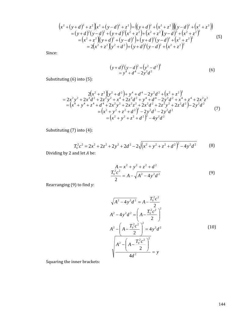
144

222222222

222222222

22222222222

222222222222

2 zxdydydyzx

zxdydydydyzx

zxdyzxzxdydydy

zxdyzxdyzdyxzdyx

(5)

Since:

2244

22222

2 dydy

dydydy

(6)

Substituting (6) into (5):

2222222

222222222

2222222222224444

22442244224222222

22222442222

4

22

222222222222

22

dydzyx

dydydzyx

dydzyzdxzxyxdzyxzxzxdydydzxyzdxyx

zxdydydyzx

(7)

Substituting (7) into (4):

2222222222222 422222 dydzyxdyzxcTV (8)

Dividing by 2 and let A be:

222

22

2222

42

dyAAcT

dzyxA

V

(9)

Rearranging (9) to find y:

yd

cTAA

dycT

AA

cTAdyA

cTAdyA

V

V

V

V

2

222

2

22

222

2

222

222

22222

4

2

42

24

24

(10)

Squaring the inner brackets:

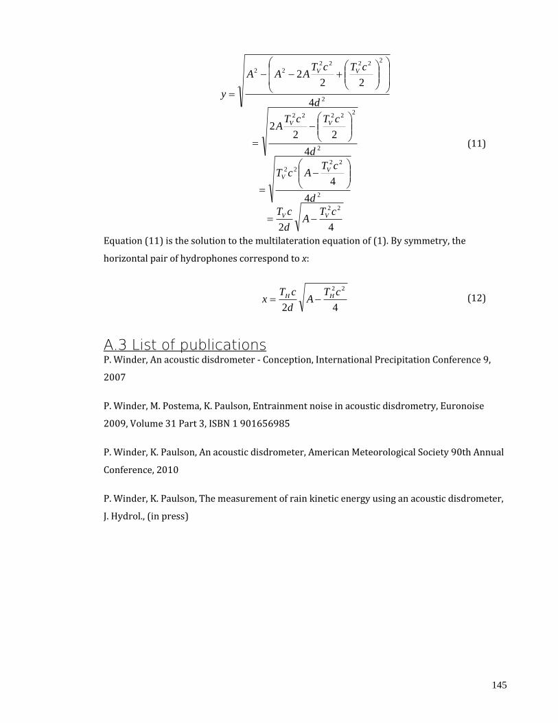
145

42

4

4

4

222

4

222

22

2

2222

2

22222

2

22222

22

cTA

d

cT

d

cTAcT

d

cTcTA

d

cTcTAAA

y

VV

VV

VV

VV

(11)

Equation (11) is the solution to the multilateration equation of (1). By symmetry, the

horizontal pair of hydrophones correspond to x:

42

22cTA

d

cTx HH (12)

A.3 List of publications P. Winder, An acoustic disdrometer - Conception, International Precipitation Conference 9,

2007

P. Winder, M. Postema, K. Paulson, Entrainment noise in acoustic disdrometry, Euronoise

2009, Volume 31 Part 3, ISBN 1 901656985

P. Winder, K. Paulson, An acoustic disdrometer, American Meteorological Society 90th Annual

Conference, 2010

P. Winder, K. Paulson, The measurement of rain kinetic energy using an acoustic disdrometer,

J. Hydrol., (in press)

146

References

Ahrens, C. D. (2008). Essentials of meteorology: an invitation to the atmosphere. Cengage

Learning.

Atlas, D., E. Amitai, and C. R. Williams (1999). Systematic variation of drop size and radar-

rainfall relations. Journal of Geophysical Research 104, 6155–6170.

Atlas, D., R. C. Srivastava, and R. S. Sekhon (1973, February). Doppler radar characteristics of

precipitation at vertical incidence. Reviews of Geophysics 11, 1–35.

Atlas, D., C. Ulbrich, and R. Meneghini (1984). The multiparameter remote measurement of

rainfall. Radio Science 19(1), 3–22.

Atlas, D. and C. W. Ulbrich (1977). Path- and area-integrated rainfall measurement by

microwave attenuation in the 1-3 cm band. Journal of Applied Meteorology 16(12), 1322–1331.

Beard, K. V. (1977). On the acceleration of large water drops to terminal velocity. Journal of

Applied Meteorology 16(10), 1068–1071.

Beard, K. V. and C. Chuang (1987, June). A new model for the equilibrium shape of raindrops.

Journal of Atmospheric Sciences 44, 1509–1524.

Beard, K. V. and H. R. Pruppacher (1969, September). A determination of the terminal velocity

and drag of small water drops by means of a wind tunnel. Journal of Atmospheric Sciences 26,

1066–1072.

Best, A. C. (1950). Empirical formulae for the terminal velocity of water drops falling through

the atmosphere. Quarterly Journal of the Royal Meteorological Society 76(329), 302–311.

Brawn, D. (2009). An Elementary Estimation of Gamma Parameters and the Analysis of

Disdrometer Data. Ph. D. thesis, Department of Mathematical Sciences, University of Essex.

Brodie, I. and C. Rosewell (2007). Theoretical relationships between rainfall intensity and

kinetic energy variants associated with stormwater particle washoff. Journal of

Hydrology 340(1-2), 40–47.

147

Burgueno, A., M. Puigcerver, and E. Vilar (1988, September). Influence of rain gauge

integration time on the rain rate statistics used in microwave communications. Annals of

Telecommunications 43(9), 522–527.

Caruthers, J. (1977). Fundamentals of marine acoustics. Elsevier.

Cole, F. (1975). Introduction to meteorology. Wiley.

Davis, A. (1934). Modern Acoustics. G. Bell and Sons Ltd.

Deng, Q., A. V. Anilkumar, and T. G. Wang (2007). The role of viscosity and surface tension in

bubble entrapment during drop impact onto a deep liquid pool. Journal of Fluid

Mechanics 578(-1), 119–138.

Ding, J., F. Tsaur, A. Lips, and A. Akay (2007). Acoustical observation of bubble oscillations

induced by bubble popping. Physical Review E 75(4), 41601.

Dingle, N. and Y. Lee (1972). Terminal fallspeeds of raindrops. Journal of Applied

Meteorology 11(5), 877–879.

Foote, G. B. and P. S. Du Toit (1969). Terminal velocity of raindrops aloft. Journal of Applied

Meteorology 8(2), 249–253.

Franz, G. J. (1959). Splashes as sources of sound in liquids. The Journal of the Acoustical Society

of America 31(8), 1080–1096.

Gunn, R. and G. D. Kinzer (1949, August). The terminal velocity of fall for water droplets in

stagnant air. Journal of Atmospheric Sciences 6, 243–248.

Guo, Y. P. and J. E. F. Williams (1991). A theoretical study on drop impact sound and rain noise.

Journal of Fluid Mechanics Digital Archive 227(-1), 345–355.

Honda (2009). Ultrasound Handbook. Honda.

H.Riehl (1978). Introduction to the atmosphere. McGraw-Hill.

Jolliffe, I. T. (2002). Principal component analysis. Springer.

Joss, J. and A. Waldvogel (1967, December). Ein spektrograph fur niederschlagstropfen mit

automatischer auswertung. Pure and Applied Geophysics 68(1), 240–246.

148

Joss, J. and A. Waldvogel (1969, May). Raindrop size distribution and sampling size errors.

Journal of Atmospheric Sciences 26, 566–569.

Joss, J. and A. Waldvogel (1977). Comments on "some observations on the joss-waldvogel

rainfall disdrometer". Journal of Applied Meteorology 16(1), 112–113.

Kaplan, I. (2010, April). Wavelets and signal processing.

http://www.bearcave.com/misl/misl_tech/wavelets/. Online.

Kay, S. (1998). Fundamentals of statistical signal processing. Volume 2: detection theory.

Prentice Hall.

Kinnell, P. (1981). Rainfall intensity-kinetic energy relationships for soil loss prediction. Soil

Sci Soc Am J 45(1), 153–155.

Kinnell, P. I. A. (1976). Some observations on the joss-waldvogel rainfall disdrometer. Journal

of Applied Meteorology 15(5), 499–502.

Kruger, A. and W. Krajewski (2002). Two-dimensional video disdrometer: A description.

Journal of Atmospheric and Oceanic Technology 19, 602–617.

Kuttruff, H. (2007). Acoustics: an introduction. Taylor & Francis.

Lanzinger, E., M. Theel, and H. Windolph (2006). Rainfall amount and intensity measured by

the thies laser precipitation monitor. In TECO-2006 WMO Technical Conference on

Meteorological and Environmental Instruments and Methods of Observation, Volume 3, pp. 4–6.

Laville, R., G. Abbott, and M. Miller (1991). Underwater sound generation by rainfall. The

Journal of the Acoustical Society of America 89(2), 715–721.

Laws, J. and D. Parsons (1943). The relationship of raindrop size to intensity. Trans. Amer.

Geophys. Union 24, 452–460.

Laws, J. D. (1941). Measurements of the fall-velocity of water-drops and raindrops.

Transactions - American Geophysical Union 22, 709–721.

Leighton, T. (1994). The Acoustic Bubble. London: Academic Press.

149

Leighton, T., P. White, and M. Schneider (1998). The detection and dimension of bubble

entrainment and comminution. The Journal of the Acoustical Society of America 103, 1825–

1835.

Lesser, M. and J. Field (1983). The impact of compressible liquids. Annual Review of Fluid

Mechanics 15(1), 97–122.

Likhterov, L. (1997). High-frequency acoustic noise emitted by initial impact of solid sphere

falling onto liquid surface. Physics of Fluids 10, 321–323.

Liu, J. and H. Orville (1969). Numerical modeling of precipitation and cloud shadow effects on

mountain-induced cumuli. Journal of the Atmospheric Sciences 26(6), 1283–1298.

Lurton, X. (2002). An introduction to underwater acoustics: principles and applications.

Springer.

Lutgens, F. and E. Tarbuck (1998). The atmosphere: an introduction to meteorology. Prentice-

Hall international editions.

Ma, B. B., J. A. Nystuen, and R.-C. Lien (2005). Prediction of underwater sound levels from rain

and wind. The Journal of the Acoustical Society of America 117(6), 3555–3565.

Mandeep, J. S. and S. I. S. Hassan (2008). 60- to 1-min rainfall-rate conversion: Comparison of

existing prediction methods with data obtained in the southeast asia region. Journal of Applied

Meteorology and Climatology 47(3), 925–930.

Mani, T. K. and P. R. S. Pillai (2004). Drop parameter estimation from underwater noise

produced by raindrop impact. Acoustics Research Letters Online 5(3), 118–124.

Manzello, S. L. and J. C. Yang (2002, May). An experimental study of a water droplet impinging

on a liquid surface. Experiments in Fluids 32(5), 580–589.

Marshall, J. S. and W. M. Palmer (1948, August). The distribution of raindrops with size.

Journal of Atmospheric Sciences 5, 165–166.

Medwin, H., A. Kurgan, and J. A. Nystuen (1990). Impact and bubble sound from raindrops at

normal and oblique incidence. The Journal of the Acoustical Society of America 88(1), 413–418.

150

Medwin, H., J. A. Nystuen, P. W. Jacobus, L. H. Ostwald, and D. E. Snyder (1992). The anatomy

of underwater rain noise. The Journal of the Acoustical Society of America 92(3), 1613–1623.

Montero-Martínez, G., A. B. Kostinski, R. A. Shaw, and F. García-García (2009, June). Do all

raindrops fall at terminal speed? Geophysical Research Letters 36, L11818.

Mott, P., C. Roland, and R. Corsaro (2002). Acoustic and dynamic mechanical properties of a

polyurethane rubber. The Journal of the Acoustical Society of America 111, 1782–1790.

Nystuen, J. (1996). Acoustical rainfall analysis: Rainfall drop size distribution using the

underwater sound field. Journal of Atmospheric and Oceanic Technology 13(1), 74–84.

Nystuen, J. and E. Amitai (2003). High temporal resolution of extreme rainfall rate variability

and the acoustic classification of rainfall. Journal of Geophysical Research-

Atmospheres 108(D8), 8378.

Nystuen, J. and D. Farmer (1987). The influence of wind on the underwater sound generated

by light rain. The Journal of the Acoustical Society of America 82, 270–274.

Nystuen, J. A. (1986). Rainfall measurements using underwater ambient noise. The Journal of

the Acoustical Society of America 79(4), 972–982.

Nystuen, J. A. (2001, October). Listening to raindrops from underwater: An acoustic

disdrometer. Journal of Atmospheric and Oceanic Technology 18, 1640–1657.

Nystuen, J. A., C. C. McGlothin, and M. S. Cook (1993). The underwater sound generated by

heavy rainfall. The Journal of the Acoustical Society of America 93(6), 3169–3177.

Ogden, R. (1997). Essential wavelets for statistical applications and data analysis. Birkhäuser.

Oguz, H. N. and A. Prosperetti (1991). Numerical calculation of the underwater noise of rain.

Journal of Fluid Mechanics Digital Archive 228(-1), 417–442.

Onof, C., R. E. Chandler, A. Kakou, P. Northrop, H. S. Wheater, and V. Isham (2000). Rainfall

modelling using poisson-cluster processes: a review of developments. Stochastic

Environmental Research and Risk Assessment 16(6), 384–411.

Ouis, D. (2005). Modelling the mechanical properties of rubber by means of a five-parameter

dispersive model. Proceedings of International Rubber Conference.

151

Paulson, K. S. and X. Zhang (2009). Simulation of rain fade on arbitrary microwave link

networks by the downscaling and interpolation of rain radar data. Radio Sci. 44.

Piezo Systems Inc. (website accessed 2010, March). Piezoceramic materials and properties.

http://www.piezo.com/prodmaterialprop.html.

Polikar, R. (2010, April). The wavelet tutorial.

http://users.rowan.edu/ polikar/wavelets/wttutorial.html. Online.

Prosperetti, A. and H. N. Oguz (1993). The impact of drops on liquid surfaces and the

underwater noise of rain. Annual Review of Fluid Mechanics 25(1), 577–602.

Pumphrey, H. (1991). Underwater rain noise - the initial impact component. Institute of

Acoustics Proceedings 13, 192–200.

Pumphrey, H. and P. Elmore (1990). The entrainment of bubbles by drop impacts. Journal of

Fluid Mechanics 220, 539–567.

Pumphrey, H. C., L. A. Crum, and L. B. rnø(1989). Underwater sound produced by individual

drop impacts and rainfall. The Journal of the Acoustical Society of America 85(4), 1518–1526.

Rafiee, J., P. Tse, A. Harifi, and M. Sadeghi (2009). A novel technique for selecting mother

wavelet function using an intelligent fault diagnosis system. Expert Systems with

Applications 36(3, Part 1), 4862–4875.

Rosen, C., B. Hiremath, and R. Newnham (1992). Piezoelectricity. Springer.

Rosewell, C. J. (1986). Rainfall kinetic energy in eastern australia. Journal of Applied

Meteorology 25(11), 1695–1701.

Salles, C. and J. Poesen (2000, February). Rain properties controlling soil splash detachment.

Hydrological Processes 14, 271–282.

Salles, C., J. Poesen, and D. Sempere-Torres (2002). Kinetic energy of rain and its functional

relationship with intensity. Journal of Hydrology 257(1-4), 256–270.

Schönhuber, M., G. Lammer, and W. Randeu (2007). One decade of imaging precipitation

measurement by 2d-video-disdrometer. Adv. Geosci. 10, 85–90.

152

Segal, B. (1986). The influence of raingage integration time, on measured rainfall-intensity

distribution functions. Journal of Atmospheric and Oceanic Technology 3(4), 662–671.

Sherman, C. and J. Butler (2007). Transducers and arrays for underwater sound. Springer.

Smith, P. (2003). Raindrop size distributions: Exponential or gamma - does the difference

matter? Journal of Applied Meteorology 42, 1031–1034.

Steiner, M. and J. A. Smith (2000, November). Reflectivity, rain rate, and kinetic energy flux

relationships based on raindrop spectra. Journal of Applied Meteorology 39, 1923–1940.

Thies Clima (2010, June). Laser precipitation monitor (disdrometer).

http://www.thiesclima.com/disdrometer.html. Online.

Thoroddsen, S. T., T. G. Etoh, and K. Takehara (2003). Air entrapment under an impacting

drop. Journal of Fluid Mechanics 478(-1), 125–134.

Uijlenhoet, R. and J. N. M. Stricker (1999). A consistent rainfall parameterization based on the

exponential raindrop size distribution. Journal of Hydrology 218(3-4), 101–127.

Ulbrich, C. W. (1983, October). Natural variations in the analytical form of the raindrop size

distribution. Journal of Applied Meteorology 22, 1764–1775.

Ulbrich, C. W. and D. Atlas (1977). A method for measuring precipitation parameters using

radar reflectivity and optical extinction. Annals of Telecommunications 32(11), 415–421.

Ulbrich, C. W. and D. Atlas (1984). Assessment of the contribution of differential polarization

to improved rainfall measurements. Radio Science Radio Sci.19(1), 49–57.

Upton, G., D. Brawn, and W. Park (2007). An investigation of factors affecting the accuracy of

thies disdrometers. Available online.

Vagle, S., W. Large, and D. Farmer (1990). An evaluation of the wotan technique of inferring

oceanic winds from underwater ambient sound. J. Atmos. Oceanic Technol 7(4), 576–595.

Van Dijk, A., L. Bruijnzeel, and C. Rosewell (2002). Rainfall intensity-kinetic energy

relationships: A critical literature appraisal. Journal of Hydrology 261(1-4), 1–23.

Walker, J. (1999). A primer on wavelets and their scientific applications. CRC Press.

153

Wang, P. K. and H. R. Pruppacher (1977). Acceleration to terminal velocity of cloud and

raindrops. Journal of Applied Meteorology 16(3), 275–280.

Weeks, M. (2010). Digital Signal Processing Using MATLAB and Wavelets. Jones & Bartlett

Learning.

Wells, N. (1997). The atmosphere and ocean: a physical introduction. Wiley.

Wobus, H. B., F. Murray, and L. Koenig (1971). Calculation of the terminal velocity of water

drops. Journal of Applied Meteorology 10(4), 751–754.

Yang, J. (2005). An introduction to the theory of piezoelectricity. Springer.