The E�ects of Recombination on a Haploid QuasispeciesEvolving on a Single-peak Fitness LandscapeLionel BarnettCentre for the Study of EvolutionCentre for Computational Neuroscience and RoboticsSchool of Cognitive and Computing SciencesUniversity of SussexBrighton BN1 9QH, UKlionelb@cogs.susx.ac.ukJanuary 24, 2000AbstractIn this paper we investigate the e�ects of (uniform) recombination on the evolution of ahaploid quasispecies on a single-peak \spike" �tness landscape. It is found that at lowmutation rates the long-term behaviour of the quasispecies exhibits one stable and oneunstable equilibrium. At a critical mutation rate which we identify as an error threshold, thestable and unstable equilibria coalesce. Beyond the error threshold there is no (biologicallymeaningful) equilibrium; errors accumulate and the optimum genotype is inevitably lost.In contrast to the asexual case where the error threshold is discontinuous, the sexual errorthreshold represents a 2nd order (continuous) phase transition. It is mooted that theunstable equilibrium could act as a barrier to the �xation of a favourable mutant. Wederive analytic approximations for the equilibrium concentrations of the optimum genotypeand for the error threshold. We also analyse the stability of the equilibria.1 IntroductionManfred Eigen, in his quasispecies formalism(Eigen, 1971; Eigen and Schuster, 1979; Eigen et al.,1989), developed an approach to analysing the evolution of large populations of information-encoding sequences based on (deterministic) ow-reactor kinetics, whereby concentrations ofsequence types change according to di�erential rates of replication, destruction and, via muta-tion, transformation to di�erent types. This formalism led to the concept of a quasispecies asa distribution of sequences localised in sequence space and clustered around the most frequentsequence variety. The existence of an error threshold of mutation (or replication �delity) wasestablished, beyond which the �ttest sequence type would inevitably be lost from the population.The implication is that if the mutation rate is too high a favourable mutant can never becomeestablished in an evolving population. Furthermore, the error threshold typically decreases withincreasing sequence length, so that there is e�ectively (for a given per-allele mutation rate) alimit to the sequence length beyond which an evolving population of sequences can maintainsu�ciently high �tness to be viable. This observation leads to the so-called \error catastro-phe"; in nature, the genomes of organisms have comparatively low e�ective per-allele mutationrates due to the existence of error correction mechanisms in e�ect during replication. However,these error correction mechanisms must themselves be coded for in the organism's genome -they are functionally non-trivial and are likely to require lengthy coding sequences, greater thanthe \raw" per-allele mutation rate would permit due to the error threshold. How, then, could1

these error correction mechanisms (and hence complex organisms requiring long genomes) haveevolved?There has been a persistent and recurrent idea that an answer to this conundrummay lie withsex and recombination (Maynard Smith, 1978; Kimura and Maruyama, 1966; Kondrashov, 1982;Charlesworth, 1990). Thus it has been suggested that, under certain circumstances, recombina-tion can act as a kind of error repair mechanism. It is, therefore, of great interest to examine thee�ects of recombination on the dynamics of a quasispecies and on error thresholds in particu-lar. In attempting to extend the \classical" quasispecies formalism to include recombination weimmediately come up against two problems. The �rst is that in the asexual case analysis of thequasispecies dynamics is greatly abetted by the (near) linearity of the system; recombinationintroduces a quadratic non-linearity. Secondly, in the asexual case (and particularly if sequencelengths are long) we are generally entitled to ignore \back-mutation" of less �t sequences to the�ttest sequence type. This simpli�es the analysis considerably, enabling us to separate out thedynamics of the concentration of the �ttest sequence variety. When recombination is present wemay still neglect back-mutation, but we cannot ignore \back-recombination" (this is in a sensethe essence of the error-correction potential of recombination) so that the dynamics of the �ttestsequence type are inextricably linked to the concentrations of types nearby in sequence space.Our approach then is to develop approximations that re ect at least qualitatively the dynamicsof the sexual quasispecies.The basic quasispecies model employed in this paper is as follows: we consider a large(e�ectively in�nite) population of haploid genotypes, considered as binary sequences of �xedlength N evolving under selection, mutation and recombination. There is a single \optimal"genotype1 and the �tness of any sequence depends only on the number of errors; i.e. theHamming distance of that sequence from the optimal sequence.We shall be interested mainly in the long sequence length limit N !1; all analytical resultsare strictly valid only in this limit. Numerical simulations are of necessity performed with �nitesequence length, although care was taken to use the longest sequence lengths compatible withclarity and feasible within the constraints of computational resources. In what follows (unlessotherwise stated) all Latin indices i; j; : : :, Greek indices �; �; : : : and summations run from 0 toN (where N may be 1).Let wi denote the �tness of a sequence with i errors. We now specialise to a \spike" �tnesslandscape de�ned by:wi = 1 + �i0� = � 1 + � if i = 01 if i > 0 (1)where � > 0 is the selection coe�cient2 of the optimum sequence. It must be remarked thatwhile this �tness landscape arguably lacks biological relevance, it has the advantage of simplicityand allows for direct comparison with known results from asexual quasispecies theory. We shallreturn to this topic in Section 6 below.We use xi(t) to denote the proportion (or concentration) of sequences with i errors at gen-eration t, so that Pi xi(t) = 1. (xi)i=1;:::;N represents the quasispecies distribution of thepopulation. We will use the generating functions gt(z) for the xi(t) de�ned by:gt(z) �Xk xk(t)(1 � z)k (2)Note that gt(0) = 1 and (by convention) gt(1) = x0. We also de�ne:�(t) �Xk kxk(t) (3)1Also known in the literature as the \wild-type" or \master sequence".2It is commonplace in the population genetics literature to take the optimum �tness as 1 and that of othergenotypes as 1� s. Since we shall only consider �tness-proportional selection, there is no essential di�erence; �and s are related by 1 + � = 11�s . 2

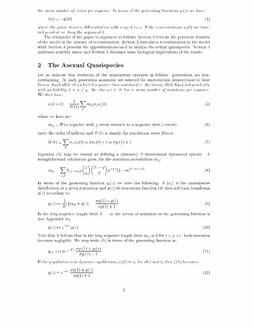
the mean number of errors per sequence. In terms of the generating functions gt(z) we have:�(t) = �g0t(0) (4)where the prime denotes di�erentiation with respect to z. If the concentrations xi(t) are time-independent we drop the argument t.The remainder of the paper is organised as follows: Section 2 reviews the pertinent featuresof the model in the absence of recombination. Section 3 introduces recombination to the modelwhile Section 4 presents the approximations used to analyse the sexual quasispecies. Section 5addresses stability issues and Section 6 discusses some biological implications of the results.2 The Asexual QuasispeciesLet us suppose that evolution of the quasispecies operates as follows: generations are non-overlapping. At each generation sequences are selected for reproduction proportional to their�tness. Each allele of a selected sequence then mutates (i.e. the binary allele ips) independentlywith probability 0 < u < 12 . We also set U � Nu = mean number of mutations per sequence.We then have:xi(t+ 1) = 1W (t)Xj mijwjxj(t) (5)where we have set:mij � P (a sequence with j errors mutates to a sequence with i errors) (6)(note the order of indices) and W (t) is simply the population mean �tness:W (t) �Xk wkxk(t) = �x0(t) + 1 = �gt(1) + 1 (7)Equation (5) may be viewed as de�ning a (discrete) N -dimensional dynamical system. Astraightforward calculation gives, for the mutation probabilities mij :mij =X�;� �i;j��+��j���N � j� �u�+�(1� u)N�(�+�) (8)In terms of the generating function gt(z) we note the following: if (xi) is the quasispeciesdistribution at a given generation and g(z) its generating function (2) then selection transformsg(z) according to:g(z) 7! 1W [�x0 + g(z)] = �g(1) + g(z)�g(1) + 1 (9)In the long sequence length limit N !1 the action of mutation on the generating function is(see Appendix A):g(z) 7! e�Uzg(z) (10)Note that it follows that in the long sequence length limit mij = 0 for i < j; i.e. back-mutationbecomes negligible. We may write (5) in terms of the generating function as:gt+1(z) = e�Uz �gt(1) + gt(z)�gt(1) + 1 (11)If the population is in dynamic equilibrium, xi(t) = xi for all i and t, then (11) becomes:g(z) = e�Uz �g(1) + g(z)�g(1) + 1 (12)3

0

0.2

0.4

0.6

0.8

1

0 20 40 60 80 100

t

x0

0

0.2

0.4

0.6

0.8

1

0 0.2 0.4 0.6 0.8 1 1.2 1.4

U

x0

σ = 0.1σ = 0.4

σ = 1.0σ = 3.0Figure 1: Genotype concentrations x0(t) forthe asexual quasispecies (5) plotted againsttime. Sequence length N = 20, selection co-e�cient � = 0:1, per-genome mutation rateU = 0:05. We note that for this value of �,Ua � 0:0953. Figure 2: Equilibria of (5) plotted against per-genome mutation rate.which may be solved directly for g(z). We �nd in particular, setting z = 1, that the optimumgenotype concentration is given by either x0 = g(1) = 0 or:x0 = g(1) = 1� �e�U (� + 1)� 1)� (13)Now x0 must be non-negative. From examination of (13) we see that, given a selection coe�cient�, there can only be an equilibrium solution with a non-vanishing concentration of the optimumgenotype if U is less than a certain critical value Ua given by:Ua = loge(1 + �) (14)This critical mutation rate has been termed an error threshold. The behaviour of the model isillustrated in Figs. 1 and 2. In Fig. 1 the optimum genotype concentration x0(t) as calculatedfrom (5) is plotted against time for U < Ua. We see that there is a single stable equilibrium.As the mutation rate is increased to the critical rate Ua the equilibrium approaches zero dis-continuously. In Fig. 2 the equilibrium optimum genotype concentrations are plotted againstper-genome mutation rate for a few selection coe�cients. The transition in the equilibrium be-haviour of the quasispecies as the parameter U crosses the error threshold Ua is of a form thatwould be recognised by physicists as a 1st order (or discontinuous) phase transition.3 The Sexual QuasispeciesWe now add recombination to the above model as follows: at each generation sequences areselected for reproduction proportional to their �tness. Selected sequences pair o� at random;each pair produces an o�spring with uniform crossover (Syswerda, 1989); i.e. each allele in theo�spring sequence is chosen independently from one of its two parents with probability 12 . Eachallele of the o�spring then mutates as before. This model is similar to the model of retrovirusreplication with superinfection presented in (Boerlijst et al., 1996). Equation (5) now becomes:xi(t+ 1) = 1W (t)2 Xj;k;lmijrjklwkwlxk(t)xl(t) (15)where we have set:rjkl � P� the o�spring of a sequence with k errors recombinedwith a sequence with l errors has j errors � (16)4

0

0.2

0.4

0.6

0.8

1

0 20 40 60 80 100

t

x0

(a)

0

0.2

0.4

0.6

0.8

1

0 100 200 300 400 500

x0

t

(b)

Figure 3: Genotype concentrations x0(t) for the quasispecies with recombination(Eq. 15) plottedagainst time. Sequence length N = 20, selection coe�cient � = 0:4 and (a) per-genome mutationrate U = 0:11, (b) U = 0:15.Note that for (16) to make sense we have to suppose that recombination probabilities do notdepend on the full distribution of all sequence types within the population, rather only on thequasispecies distribution. This will be the case if the population is in linkage equilibrium, whichwe explicitly assume. Now it is well-known that linkage equilibrium is reinforced by recombina-tion and mutation but tends to be destroyed by �nite population drift (Crow and Kimura, 1970;Maynard Smith, 1998). To test the assumption Monte Carlo simulations were run with �nitepopulations of binary sequences for population sizes in the range of 100 � 10; 000 genotypes,under the evolutionary algorithm described above. The results indicated that for a wide rangeof parameter values the population remains close to linkage equilibrium and that, furthermore,the in�nite-population model provides a good approximation to the �nite-population (stochas-tic) dynamics (but see also Section 5 below). Assuming linkage equilibrium it is not di�cult toshow that:rjkl =X� �k���N � kl � � ��Nl ��1�k + l � 2�j � � ��12�k+l�2� (17)(note that this is actually symmetric in k; l).Analogous to (10), in the long sequence length limit N !1 the action of recombination onthe generating function is given by (see Appendix B):g(z) 7! g( 12z)2 (18)We may thus write (15) in terms of the generating function as:gt+1(z) = e�Uz ��gt(1) + gt( 12z)�gt(1) + 1 �2 (19)At equilibrium (19) becomes:g(z) = e�Uz ��g(1) + g( 12z)�g(1) + 1 �2 (20)Unlike (12) we cannot solve this equation explicitly for g(z) or indeed for x0 = g(1). We can,however, simulate (15) numerically. The results are illustrated in Fig. 3. Here the optimumgenotype concentration x0(t) as calculated from (15) is plotted against time. For the initialconditions binomial quasispecies distributions were chosen (see Section 4 below for justi�cation).We see that at the lower mutation rate the dynamical system (15) apparently has a stableequilibrium (at x0 � 0:6) and an unstable equilibrium (at x0 � 0:1). There is also apparently astable equilibrium at x0 � 0, but we shall argue (see Section 6) that this equilibrium cannot be5

biologically meaningful. At the higher mutation rate only the (unrealistic) x0 � 0 equilibriumremains. At a critical per-genome mutation rate Us between these values the system bifurcates,the unstable and stable equilibria coalescing and vanishing. We identify this critical mutationrate as an error threshold since beyond this value the optimumgenotype concentration inevitablyfalls to (nearly) zero. Again, a physicist would recognise this transition as a 2nd order (orcontinuous) phase transition.4 Approximations for the Sexual QuasispeciesSimulation of the sexual quasispecies model indicates that, due to the \shu�ing" e�ect of recom-bination, the quasispecies distribution rapidly attains (from any initial conditions) a distributionclose to a binomial distribution, which, in the long sequence length limit approaches a Poissondistribution. We thus proceed as follows: taking at generation t the Poisson distribution:xk(t) = e��(t) �(t)kk! (21)with generating function:gt(z) = e��(t)z (22)the evolutionary equation (15) yields for the next generation a distribution which will be \nearlyPoisson". We approximate this distribution by another Poisson distribution, choosing �(t + 1)judiciously. This we shall do in two ways, according as the selection coe�cient � is small or large;in either case we e�ectively reduce the evolution of the quasispecies from an N -dimensional toa 1-dimensional dynamical system.4.1 Small-� ApproximationIf � is small, the evolution of the quasispecies from one generation to the next was foundempirically to be dominated by the mean number of errors �(t). For the long sequence lengthlimit we thus choose �(t + 1) to be the mean number of errors one generation on, starting witha Poisson distribution (21) at generation t. Substituting gt(z) from (22) in the right hand sideof (19) then using the relation (4) we �nd immediately:�(t + 1) = U + �(t)�e��(t) + 1 (23)The equilibrium condition �(t) = �(t + 1) = : : : = � yields, after rearranging terms:e�� = U� 1� � U (24)which may be solved numerically for x0 = e��. Equation (24) is observed to have two solutionsfor U smaller than a threshold value bUs which approximates the error threshold Us of the exactmodel (15) for small �.We can calculate the approximate error threshold bUs as follows: the two solutions for �of (24) correspond to the points where the curves f(�) = e� and g(�) = �U (� � U ) intersect.At the approximate error threshold U = bUs these curves are tangential; i.e. f(�) = g(�) andf 0(�) = g0(�). Solving these equations we �nd that bUs is the (unique) solution of:UeU+1 = � (25)which may be solved numerically for bUs in terms of �. We note that for small �, bUs is of thesame order as � and we have:bUs = �e +O ��2� (26)6

This may be compared with Ua = �+O ��2� for the asexual case (14). It is also not di�cult toshow that at the error threshold:x0 = 1e +O (�) (27)4.2 Large-� ApproximationIf � is large, the evolution of the quasispecies was found to be dominated by the optimumgenotype concentration x0(t). We proceed as for the small-� case, except that we now choose�(t + 1) such that x0(t + 1) = e��(t+1) is the optimum genotype concentration in the nextgeneration, again starting with the Poisson distribution (21) at generation t. Substituting gt(z)from (22) in the right hand side of (19), setting z = 1 and noting that x0(t) = e��(t) we �nd:x0(t + 1) = e�U �x0(t) +px0(t)�x0(t) + 1 !2 (28)At equilibrium, x0(t) = x0(t + 1) = : : : = x0, we �nd (assuming x0 > 0 and taking square rootsof both sides):�x0 + 1 = e� 12U (�px0 + 1) (29)This is a quadratic equation for px0 which may be solved explicitly, yielding two values for x0so long as U is less than a critical value eUs which approximates the error threshold Us of theexact model (15) for large �. eUs is easily found to be:eUs = �2 loge� 2� (p1 + � � 1)� (30)For large � we see that eUs scales as:eUs = loge �4 + O��� 12 � (31)so that Ua � eUs = loge 4 + O��� 12� � 1:3863 for large �. We also �nd that at the errorthreshold:x0 = 1�2 (� � 2p1 + �) (32)which, for large �, scales as:x0 = 1� + O��� 32 � (33)In Fig. 4 we plot optimum genotypes concentration x0 for the equilibria of (15) with N = 60,against per-genome mutation rate U for several values of the selection coe�cient �. The small-and large-� approximations (24), (29) for x0 are plotted on the same graph. In this �gure theupper branches of the curves represent the stable and the lower branches the unstable equilibria.It was also found that for any �; U the optimum genotype concentration x0 at equilibrium isalways smaller with recombination than without.Fig. 5 plots the error threshold Us computed from numerical simulation of (15) with sequencelength N = 80 as well as the small- and large-� approximations bUs and eUs against �. The asexualerror threshold Ua is also plotted for comparison.7

0

0.2

0.4

0.6

0.8

1

0 0.1 0.2 0.3 0.4 0.5 0.6 0.7

U

x0 σ = 0.1 σ = 0.4 σ = 1.0 σ = 2.0

simulation (N = 60)small-σ approximationlarge-σ approximation

Figure 4: Equilibria of (15) and approximations (24), (29) plotted against per-genome mutationrate.0

0.5

1

1.5

2

2.5

3

1 2 4 8 16

1+σ (log scale)

U

simulation (N = 80): Ussmall-σ approximation:

^Us

large-σ approximation: ~Us

asexual: Ua

Figure 5: Error thresholds Us, bUs, eUs and Ua plotted against 1 + � (note logarithmic scale).8

(a)

0100

200300

400500

600

t0

510

1520

i (errors)

0

0.1

0.2

0.3

0.4

0.5

0.6

xi (b)

0100

200300

400500

600

t0

510

1520

i (errors)

0

0.1

0.2

0.3

0.4

0.5

0.6

xi

Figure 6: Behaviour of the sexual quasispecies near the unstable equilibrium. In both casesN = 20, � = 0:4, U = 0:11 and the population was initialised with a binomial distribution (a)just above and (b) just below the unstable equilibrium.5 Stability of EquilibriaWe wish to investigate the stability of the equilibrium solutions to (15). This is of particularimportance to analysis of �nite-population models for which (15) may be an approximation,since stochastic uctuations will occur in the concentrations xi(t) which might destabilise adeterministic equilibrium. Furthermore, we note that, particularly for small �, the system maypersist in a state apparently close to the unstable equilibrium for a considerable time beforedestabilising (Fig. 6); we should like to elucidate the mechanism by which these \nearly stable"quasispecies destabilise.Consider a discrete dynamical system:x(t + 1) = F (x(t)) (34)where x is a real vector (xi) and F (x) a (smooth) vector-valued function with componentfunctions Fi(x). Suppose further that � is a �xed-point of (34); i.e.:� = F (�) (35)Suppose now that at time t, x(t) is close to �; i.e. � � jx(t) � �j is small. We �nd then from(34) and (35) that:x(t + 1)� � = rF (�) � (x(t)� �) + o (�) (36)where rF (�) is the matrix with components @Fi@xj ����x=� and (36) is the linearisation of the dy-namical system (34) about the �xed-point �. It represents the linear transformation mappingpoints in the vicinity of a �xed-point to their positions in the next generation. Now the prin-cipal eigenvalue of a linear transformation indicates the degree of \stretching" in the directionof greatest stretching; a �xed-point of a dynamical system (34) will be stable i� j�0j < 1 where�0 is the principal eigenvalue of rF at that �xed-point. Our evolutionary equations (15) are ofthe form (34) with F given by:Fi(x) = 1W (x)2 Xj;k;lmijrjklwkwlxkxl (37)with the added constraint Pi xi = 1. We �nd that at a �xed-point �:[rF (�)]ij = 2wjW (�) 8<:��i + 1W (�)Xk;l milrljkwk�k9=; (38)9

0.3

0.4

0.5

0.6

0.7

0.8

0.9

1

1.1

1.2

0 0.1 0.2 0.3 0.4 0.5 0.6

U

λ0

σ = 0.1

σ = 0.4

σ = 1.0

σ = 2.0Figure 7: Principal eigenvalues of rF (�) for the stable (lower branches) and unstable (upperbranches) equilibria of (15). Sequence length N = 60.To analyse the linear transformationrF (�) given by (38) we calculated its eigenvalues �0 > �1 >�2 > : : : > �N = 0 for the stable and unstable equilibria3. Fig. 7 plots the principal eigenvalues�0 for a range of mutation rates and a few � values, for the stable (lower branches) and unstable(upper branches) equilibria. It was also found empirically that the remaining eigenvalues fall o�roughly exponentially; i.e. for �xed � and U there is a constant c � 12 such that for k = 1; 2; : : :we have �k � ck�0. It was certainly the case that for the stable equilibrium j�0j < 1 (con�rmingstability) while for the unstable equilibrium j�0j > 1 (con�rming instability) and that in bothcases j�kj < 1 for k > 0. This latter implies in particular that the unstable equilibrium of (15)is only unstable along a single dimension - we might think of it as a narrow steep-walled saddle-shaped gully with a shallow curvature in the direction of the principal eigenvector of rF (�). Forsmall � (see Fig. 7 and analysis below) we see that �0 is only slightly larger than 1. This explainsthe comparative stability of the unstable equilibrium (Fig. 6). It is also interesting to note thatfor a given selection coe�cient � there is a critical mutation rate at which the instability of theunstable equilibrium is greatest. For higher mutation rates the unstable equilibrium becomesless unstable as the error threshold is approached.To approximate the principal eigenvalues, we proceed as follows: in Section 4 we approxi-mated the N -dimensional system (15) by the 1-dimensional systems (23) and (28). Considerthe general situation where there is a vector function �(y) = (�i(y)) of a new variable y and ascalar function f(y) satisfying the relation �(f(y)) = F (�(y)) 8 y or, in functional notation:� � f = F �� (39)This equation4 formalises the notion of \reducing the dimension" of the dynamical system (34)3It was found (although not proven analytically) that all eigenvalueswere non-negative. We note thatPi xi =1 implies that rF (�) is a projection, so that there must exist at least one zero eigenvalue.4In mathematical \Category Theory" Equation (39) would de�ne � as an endomorphism within the categoryof (discrete) dynamical systems. 10

to the new 1-dimensional dynamical system y(t + 1) = f(y(t)). We then have:�0i(f(y))f 0(y) =Xj Fi;j(�(y))�0j (y) 8 y (40)where primes denote di�erentiation, so that if � is a �xed-point of f then f 0(�) is an eigenvalueof rF (�) for � = �(�), with eigenvector �0(�).The small-� approximation of Section 4.1 is an approximation to just such a reduction ofdimension (in the sense that the relation (39) is \almost" satis�ed) if we identify y with �.�(�) is then speci�ed by (21) and f(�) by (23). The eigenvalue �̂0 � f 0(�) at the stable (resp.unstable) �xed-point � is found to be:�̂0 = (1 + U )�1� U� � (41)where � represents the stable (resp. unstable) solution of the equilibrium equation (24).For the large-� approximation of Section 4.2 we identify y with x0; �(x0) is then speci�edby (21) and f(x0) by (28). The eigenvalue ~�0 � f 0(x0) at the stable (resp. unstable) �xed-pointx0 is found to be:~�0 = 2� e� 12U�x0 + 1 (42)where x0 represents the stable (resp. unstable) solution of the equilibrium equation (29).Numerical computation of �̂0 and ~�0 showed them to be reasonable approximations to theprincipal eigenvalue �0 of rF (�) (for both stable and unstable equilibria) for small and largevalues of � respectively. We may also conclude that for small � the unstable equilibrium is mostsensitive to perturbations of �, the mean number of errors per sequence, while for large � it ismore sensitive to perturbations of x0.Finally, we return to a remark made in the Section 3, namely that the in�nite-populationmodel (15) is generally a good approximation to the corresponding �nite-population (stochastic)model. This is not entirely true near the unstable equilibrium; unsurprisingly stochastic uctu-ations will tend to dislodge the population from the vicinity of the unstable equilibrium, whencethe population will either converge to the stable equilibria or errors will accumulate with loss ofthe optimum genotype (Fig. 8).6 DiscussionBefore discussing the implications of the results presented here, some remarks are in order aboutthe �tness landscape. Several charges of biological implausibility might be leveled against our\spike" landscape. One is that it seems unlikely that there should be just a single optimumgenotype and that all genotypes just a few mutations away from that optimum should haveequal lower �tness; conventional wisdom has it that as mutations accumulate �tness shoulddrop o� according to some scheme (often taken to be multiplicative).Perhaps a more serious charge is that it seems highly unlikely that any number of mutationscould accumulate without impacting �tness. This will happen when the quasispecies distributiondestabilises, in particular when the mutation rate is higher than the error threshold. This maybe observed in Fig. 6b where after destabilisation the quasispecies distribution moves o� ina \wave" towards a higher number of errors5. It is for this reason that we must reject the\near zero" optimum concentration in the �nite sequence length case as a plausible equilibrium.Of course in the in�nite sequence length idealisation there is no equilibrium at all - the \wave"simply keeps on moving. It should be noticed, furthermore, that in our derivation of the formulaefor mutation and recombination probabilities in the in�nite sequence length limit (AppendicesA, B), the number of errors is held �xed during passage to the limit; for long (but �nite) sequence5This phenomenon was correctly predicted by John Maynard Smith (private communication).11

0

0.2

0.4

0.6

0.8

1

0 200 400 600 800 1000

t

x0

finite populationinfinite population

Figure 8: Optimum genotype concentration plotted against time for two typical simulatonsof a �nite population (stochastic) sexual quasispecies initialised near the unstable equilibrium,alongside the corresponding in�nite-population model (15). Sequence length is N = 80, selec-tion coe�cient � = 0:4, per-genome mutation rate U = 0:1 and population size for the �nitepopulation runs is 10,000.12

lengths we should thus not expect our analytical model to furnish a good approximation if thereare appreciable concentrations of genotypes with accumulations of errors comparable to thesequence length.To test whether this last objection could perhaps be dispensed with we tried, for long sequencelengths, setting the �tness of any genotype with errors at more than e.g. 5% of the number ofloci to zero; e�ectively any mutation beyond a �xed number would be lethal. It was foundthat except for very small selection coe�cients and provided the quasispecies doesn't destabilisethe e�ect of this alteration was surprisingly slight - perhaps less surprising if we recall that,according to our analysis, the concentration of genotypes falls o� roughly exponentially withincreasing number of errors, so that genotypes with signi�cant accumulations of errors are notin any case contributing much to the behaviour of the model. Allied to this, we might also notethat, in line with (45) the contribution of recombination falls o� roughly exponentially with thenumber of errors in either parent sequence.Comparing the behaviour of the sexual with the asexual quasispecies there are several strikingfeatures. In particular it seems clear that on the spike �tness landscape recombination is adistinct disadvantage for several reasons:� The error threshold is lower with recombination than without.� Even below the error threshold the optimum genotype concentration x0 (and hence thepopulation mean �tness W ) is lower with recombination than without.� Suppose that in a �nite population our optimum genotype has been recently discovered bymutation/recombination. Even if any copies of the optimumgenotype survived eliminationby random drift, the concentration of the optimum genotype would have to rise above thelevel of the unstable equilibrium before selection could begin to \pull" it towards �xation- in the meantime mutation and recombination conspire to reduce the concentration. Inparticular, in a large population it is di�cult to see how the optimum could ever �xate.We should note that these conclusions do not contradict the theory propounded by Kondrashovand others (Kimura and Maruyama, 1966; Kondrashov, 1982; Charlesworth, 1990) that recom-bination can lead to a lower mutational load, since this is only claimed in the presence ofsynergistic epistasis; our spike landscape represents almost the opposite end of the spectrumto synergistic epistasis. Although by setting the �tness of the \error tail" to zero as describedabove our �tness landscape appears to acquire synergistic epistasis (i.e. it becomes technicallysub-multiplicative), as long as the population doesn't destabilise it essentially only \sees" thenon-synergistic portion of the landscape so that Kondrashov's principle is not violated.Another striking di�erence is the following: in the asexual case, if the quasispecies is inequilibrium just within the error threshold we would expect to see a low concentration x0 ofthe optimal genotype (Equation (13) and Fig. 2). With recombination, we would expect tosee a substantial concentration of the optimal genotype (Fig. 4), particularly if the selectioncoe�cient � is small when from (27) we have x0 � 1=e � 0:3679. Thus if we observed a sexualpopulation in equilibrium to have a reasonably high concentration of the optimum genotype wecould not infer, as we might in the asexual case, that the mutation rate was well within the errorthreshold; in e�ect, a small change in mutation rate or selection pressure could push a seeminglystable sexual population catastrophically over the error threshold.Finally, it was remarked in Section 3 that our model is similar to that in (Boerlijst et al.,1996). The principal di�erence is that in their model recombination occurs only with a givenprobability. They also consider �tness landscapes with a \plateau" of higher �tness around theoptimum genotype as well as an isolated �tness spike. They found that in certain parameterregimes their model exhibited bistability (i.e. two stable equilibria). It seems, however, thatin those cases their lower-�tness equilibrium corresponds to an unstable quasispecies which wehave argued here should be rejected as a plausible equilibrium; further research is required.In particular, we hope to extend the analysis presented here to variable recombination ratesand to landscapes featuring a plateau-like optimum - it is expected that results might di�ersubstantially, since \back-recombination" would be expected to exert a more marked e�ect. Wealso intend to investigate more fully the implications of the model for �nite populations.13

AcknowledgementsThe author would like to thank Inman Harvey and Prof. John Maynard Smith for helpfuldiscussions.A Transformation of g(z) by MutationFrom (8) we have for any z and �xed U � Nu:Xi mij(1� z)i = X�;� �j���N � j� �u�+�(1� u)N�(�+�)(1� z)j��+�= X� �j��u�(1� u)j��(1� z)j��� X� �N � j� �u�(1� z)�(1� u)N�j��= (1� z + uz)j(1� uz)N�j= �1� 1N Uz�N �1� z + 1NUz1� 1NUz �j! e�Uz(1� z)j as N !1holding j �xed, where in the last step we have used �1� 1NUz�N ! e�Uz as N ! 1. Theresult follows immediately.B Transformation of g(z) by RecombinationLet us set:cjk;� � �j���N � jk � ���Nk��1 (43)Note that cjk;� is symmetric in j; k. Then from (17) we have:rijk =X� cjk;��j + k � 2�i � � ��12�j+k�2� (44)Now using Stirling's formula (Stirzaker, 1994) it is not di�cult to show that, holding j; k and ��xed we have limN!1 cjk;� = ��0. Thus, holding i; j and k �xed, we have:limN!1 rijk = �j + ki ��12�j+k (45)[c.f. Kimura and Maruyama (1966) - this is equivalent to neglecting the probability of homozy-gous mutant alleles occurring at any locus during recombination]. In the limit:Xi rijk(1� z)i = (1� 12z)j+k (46)and the result follows. 14

ReferencesBoerlijst, M. C., Bonhoe�er, S., and Nowak, M. A. (1996). Viral quasi-species and recombination.Proc. R. Soc. Lond. B., 263:1577{1584.Charlesworth, B. (1990). Mutation-selection balance and the evolutionary advantage of sex andrecombination. Genet. Res., 55:199{221.Crow, J. F. and Kimura, M. (1970). An Introduction to Population Genetics Theory. Harperand Row, New York.Eigen, M. (1971). Selforganization of matter and the evolution of biological macromolecules.Natuurwissenschaften, 10:465{523.Eigen, M., McCaskill, J., and Schuster, P. (1989). The molecular quasispecies. Adv. Chem.Phys., 75:149{263.Eigen, M. and Schuster, P. (1979). The Hypercycle - a Principle of Natural Selforganization.Springer, New York.Kimura, M. and Maruyama, T. (1966). The mutational load with epistatic gene interactions in�tness. Genetics, 54:1337{1351.Kondrashov, A. S. (1982). Selection against harmful mutations in large sexual and asexualpopulations. Genet. Res., 40:325{332.Maynard Smith, J. (1978). The Evolution of Sex. Cambridge University Press, Cambridge, UK.Maynard Smith, J. (1998). Evolutionary Genetics. Oxford University Press, Oxford.Stirzaker, D. (1994). Elementary Probability. Cambridge University Press.Syswerda, G. (1989). Uniform crossover in genetic algorithms. In Scha�er, J. D., editor, Pro-ceedings of the Third International Conference on Genetic Algorithms and their Applications,pages 2{9. Morgan Kau�man.

15