the waccfor kpn and ftth - autoriteit consument & markt · 2015-07-08 · an ftth network. we...

The WACC for KPN and FttH

PREPARED FOR

ACM

PREPARED BY

Dan Harris

Cosimo Fischietti

Ying-Chin Chou

1 July 2015

This report was prepared for the ACM. All results and any errors are the responsibility of the

authors and do not represent the opinion of The Brattle Group, Inc. or its clients.

Copyright © 2015 The Brattle Group, Inc.

i | brattle.com

Table of Contents

I. Introduction and Summary ......................................................................................................... 1

II. KPN WACC ................................................................................................................................. 5

II.A. Cost of Debt ........................................................................................................................ 5

II.B. Gearing................................................................................................................................ 7

II.C. The Risk Free Rate ............................................................................................................. 9

II.D. Beta ................................................................................................................................... 10

II.D.1. Market Indices ............................................................................................... 10

II.D.2. Rolling Beta ................................................................................................... 10

II.D.3. Vasicek adjustments ...................................................................................... 12

II.D.4. Un-levering and Re-levering Beta ................................................................ 13

II.E. The Equity Risk Premium ............................................................................................... 14

II.F. Inflation ............................................................................................................................ 17

II.G. Summary Of KPN WACC ............................................................................................... 18

III. WACC For The Fibre-To-The-Home ...................................................................................... 18

III.A. The Search for an FttH Peer Group ................................................................................ 19

III.B. Precedent from Regulatory Decisions............................................................................. 20

III.C. FttH WACC In the DCF Model ...................................................................................... 23

APPENDIX I – Details On KPN’s Leverage ...................................................................................... 29

APPENDIX II – FttH Peer Group Analysis ....................................................................................... 31

1 | brattle.com

I. Introduction and Summary

The Dutch Authority for Consumers and Markets (ACM) needs to apply a Weighted Average

Cost of Capital (WACC) for regulating a range of telecom related services, and for carrying

out its duty of economic oversight of other telecoms activities. In this context, the ACM has

commissioned The Brattle Group to calculate the WACC for:

1. KPN Telecom;

2. Fibre-to-the-Home (FttH);

The ACM has asked us to apply its WACC methodology for KPN. We also applied this

methodology in a May 2013 report where we estimated the WACC for wholesale broadband

(in practise KPN’s WACC) and also for Fibre-to-the-Office (FttO).1 In this report, we update

our May 2013 estimate of the KPN’s WACC, and develop a new methodology for estimating

the WACC for FttH. The ACM has asked us to estimate the WACC based on the latest data

available.

In broad terms, the methodology for KPN’s WACC applies the Capital Asset Pricing Model

(CAPM) to calculate the cost of equity. The CAPM expresses the cost of equity for a business

activity as the sum of a risk-free rate and a risk premium. The size of the risk premium

depends on the systematic risk of the underlying asset, or project, relative to the market as a

whole.2

The risk-free rate is calculated based on the three-year average yield on 10-year Dutch and

German government bonds. This results in a risk-free rate of 1.49%. The ERP is calculated

using long-term historical data on the excess return of shares over long-term bonds, using

data from European markets, and considering other evidence on the ERP from Dividend

Growth Models. In more detail, the methodology specifies that the projected ERP should be

based on the average of the arithmetic and geometric average realised ERP. In the current

case, we have applied the ‘raw’ historical ERP without making any of the standard downward

adjustments. Hence, in effect we have increased our estimate of the ERP because of evidence

1 The WACC for Wholesale Broadband and FttO, The Brattle Group, Dan Harris and Cosimo

Fischietti, 29 May 2013. Hereafter referred to as the ‘May 2013 report’.

2 Further information on assumptions and theory underlying the CAPM can be found in most

financial textbooks; see Brealey, Richard; Myers, Stewart; Allen, Franklin; “Principles of Corporate

Finance.

2 | brattle.com

from dividend growth models, relative to a situation where we apply the standard downward

adjustments. This results in an ERP over bonds of 5.0%.

KPN’s recent financial history presents some specific issues when estimate a forward looking

gearing and beta. As we explained in our May 2013 report, during 2012-2013 in particular,

KPN’s share price declined and its gearing increased to high levels. KPN eventually restored

financial balance by undertaking a €4 billion rights issue. However, the last three years have

involved substantial fluctuations in KPN’s gearing. Accordingly, to estimate KPN’s likely

future gearing, we use KPN’s latest actual gearing of 42%, rather than an average of the last

three years (58%). We also find evidence that KPN’s financial difficulties have depressed its

beta, an effect we noted in our May 2013 report. In the May 2013 report, we estimated KPN’s

beta by looking at the betas of similar firms or ‘peers’. In the current report, our preferred

option is to estimate KPN’s future beta by using a two-year daily sampling period which

excludes the period of KPN’s financial difficulties, rather than using the three-year period

specified by the method. Using a two-year daily sampling period results in an asset beta of

0.45, and an equity beta of 0.69. Table I-1 summarises the overall parameters of the WACC

calculation, which yield a nominal pre-tax WACC of 6.06%. The methodology requires that

the nominal WACC is converted to a real WACC using an estimate of inflation based on both

past and predicted inflation. We convert the nominal WACC to a real WACC using an

inflation estimate of 1.5%, which results in a real WACC of 4.49%.

Table I-1: KPN’s Current WACC

2014 tax rate [1] 25.00% KPMG corporate tax table

Debt/Asset [2] 42.00% Section II.B

Debt/Equity [3] 72.41% [2]/(1-[2])

Asset beta [4] 0.45 Section II.D

Equity beta [5] 0.69 [4]x(1+(1-[1])x[3])

Risk free rate [6] 1.49% Section II.C

ERP [7] 5.00% Section II.E

After-tax cost of equity [8] 4.96% [6]+[5]x[7]

Pre-tax cost of debt [9] 5.30% Section II.A

Nominal after-tax WACC [10] 4.54% (1-[2])x[8]+[2]x(1-[1])x[9]

Nominal pre-tax WACC [11] 6.06% [10]/(1-[1])

Inflation [12] 1.50% Assumed

Real pre-tax WACC [13] 4.49% (1+[11])/(1+[12])-1

3 | brattle.com

WACC FOR FttH

In our May 2013 report we noted that the WACC for FttO is likely to be higher than the

WACC for wholesale broadband (KPN’s WACC), because of the higher ratio of fixed to

variable costs (so called operating leverage) in a newer fibre network relative to a mature

copper network.

However, there are reasons to think that FttH may have even higher systematic risk than

FttO. This is mainly because FttO tends to be built ‘on demand’ whereas FttH is built in

anticipation of demand, and is therefore more vulnerable to lower outturn demand due to for

example an economic shock.

We were unable to find a ‘pure play’ listed FttH operator form which we could estimate a

WACC directly. As a result we have investigated reasonable ways to modify the KPN’s

WACC to make it suitable for the FttH activity.

We have reviewed statements by the European Commission and decisions of other telecoms

regulators with respect to FttH. The Commission recommended that regulators apply a

premium to the WACC for investments in FttH, but to date only France, Spain, Italy and

Lithuania have implemented this recommendation. Risk premiums for FttH are 5.0% in

France, 4.81% in Spain and 4.4% in Italy. Lithuania does not disclose the size of the fibre

WACC premium it applies. However, we note that these premia compensate operators not

only for the higher systematic risk of FttH investment but also for non-systematic investment

risks, including “uncertainty relating to the costs of deployment, civil engineering works and

managerial execution”. In this exercise, we are aiming to estimate the premium required to

compensate for systematic risk only – that is, risk that an investor could not reduce by

holding a diverse portfolio of projects and shares.

To test whether premia for FttH applied by other regulators would be reasonable in the

Dutch context, we have used KPN’s Discounted Cash Flow (DCF) model of an investment in

an FttH network. We investigate the effect of both a lower than expected final adoption rate

for FttH rate and a delayed adoption of FttH on the Internal Rate of Return (IRR) of an FttH

investment. We find that a reduction in the final adoption rate from 60% to 40% will reduce

the IRR of the project from 7.85% to 3.50%. This drop of just over four percentage points is

consistent with the premia offered by other European telecoms regulators.

However, in our view the drop in the IRR reflects not only systematic risk but also the risk

that telecom operators have overestimated customers demand for FttH more generally. A

scenario which seems to better reflect systematic risk is one where the ultimate adoption rate

4 | brattle.com

is the same as the base case, but where the final adoption rate is reached three years later than

the base case due to an economic shock. This scenario lowers the IRR by about 2 percentage

points, suggesting a premium of 2 percentage points could be justified. However, this is only

correct if the delay will occur with 100% certainty. If the chance of an economic delay is

only 50%, then a premium of only 1% would seem justified.

We also note that in our May 2013 report we recommended a premium for FttO of 1

percentage point, and that the risk premium we estimate for FttH in this report should be

added to the FttO premium. This is because the FttH activity has the same systematic risks

that we identified for FttO – for example increased operating leverage because of large

investment commitments – plus additional systematic risks which are captured by the 1

percentage point premium we discuss above. Given this, and the premia established for FttH

by other regulators, we recommend a premium of two percentage points for the FttH WACC

over the KPN WACC. The two percentage point premium over the KPN WACC can be

thought of as the 1 percentage point premium already identified for FttO, plus another 1

percentage point to compensate for the additional systematic risks that apply to FttH. We

note that our estimation is lower than FttH premia recommended by the other NRAs.

However, this is because their premia include both systematic and non-systematic risk while

our goal is to quantify only the systematic risk related to the FttH activity.

5 | brattle.com

II. KPN WACC

II.A. COST OF DEBT

The ACM methodology specifies that we should use KPN’s actual or ‘embedded’ cost of debt

when estimating the WACC. Accordingly, as in the May 2013 report, we have calculated

KPN’s cost of debt as the weighted average coupon cost of all Euro denominated KPN bonds

outstanding as of 21st April 2015. We do not account for the cost of non-Euro denominated

debt. The logic is that bonds issued in non-Euro currencies are for KPN’s own risk, and that if

the interest rate on these bonds is higher or lower than that on Euro nominated bonds, then

the cost or benefit of this should not be reflected in the WACC that ACM will apply for

regulatory purposes. This results in a weighted average debt cost of 5.15%, as calculated in

Table II-1.

Table II-1: KPN’s Embedded Cost of Debt as of 21/04/2015

The methodology specifies an additional allowance of 15 basis points to cover the costs of

issuing debt, for example banking, legal and agency fees. Hence, the final cost of debt is

5.30%.

If we were calculating the cost of debt using the yield to maturity on KPN’s traded bonds,

then we would only include ‘bullet’ bonds with definite maturity dates.3 This is because other

3 A ‘bullet bond’ makes a final payment of the face value of the bond at a defined date.

Date of issue Maturity Type Currency S&P rating Outstanding Coupon rate EUR bonds EUR bullet

€million %

[A] [B] [C] [D] [E] [F] [G] [H] [I]

Outstanding KPN bonds as of 21 April 2015

22-Jun-2005 22-Jun-2015 Bullet EUR BBB- 1,000 4.00

13-Nov-2006 17-Jan-2017 Bullet EUR BBB- 750 4.75

2-Apr-2008 15-Jan-2016 Bullet EUR BBB- 645 6.50

4-Feb-2009 4-Feb-2019 Bullet EUR BBB- 750 7.50

30-Sep-2009 30-Sep-2024 Bullet EUR BBB- 607 5.63

21-Sep-2010 21-Sep-2020 Bullet EUR BBB- 723 3.75

15-Sep-2011 4-Oct-2021 Bullet EUR BBB- 500 4.50

1-Mar-2012 1-Mar-2022 Bullet EUR BBB- 615 4.25

1-Aug-2012 1-Feb-2021 Bullet EUR BBB- 361 3.25

14-Mar-2013 n/a Perpetual EUR BB 1,100 6.13

EUR bonds

Total (€million) [1] 7,051 5,951

Wtd average (%) [2] 5.15 4.96

Admin fees (%) [3] 0.15 0.15

Cost of debt (%) [4] 5.30 5.11

Notes and sources:

[A] to [F]: Outstanding KPN bonds denominated in euros as of 21/04/2015.

[1]: Sum [F]. [H] includes all EUR bonds whereas [I] includes only EUR Bullet bonds.

[2]: Weighted average [G] by [F]. [H] includes all EUR bonds whereas [I] includes only EUR Bullet bonds.

[3]: Assumed.

[4]: [2]+[3].

6 | brattle.com

types of bonds have either variable or uncertain maturity dates, which give bonds different

risk profiles and hence result in different interest rates that are not associated with the risk of

underlying business.4 The average debt cost for bullet bonds is 4.96%, which is lower than

the overall debt cost, 5.15%. However, since this is an embedded cost of debt calculation, we

include all the outstanding bonds in the estimation for the cost of debt.

Figure 1 illustrates that about €1 billion of debt may be re-financed in 2015. We have derived

a forward curve for the current cost of debt for Eurozone firms with a Standard & Poors

(S&P) Credit rating of BBB, similar to KPN’s rating.5 Figure 1 illustrates that an allowed cost

of debt of 5.30% would allow KPN to make a substantial financial gain from refinancing debt,

since KPN’s allowed cost of debt is over 450 basis points higher than we would expect a BBB

rated firm to pay.

4 A perpetual bond has no specified maturity date but is usually callable with a protection period.

This means that the bond issuer could redeem the bond at some point after the protection period

expires.

5 Forward curve is derived based on bond yields for BBB-rated, euro-denominated bonds for

European industries. We use bond yields from 01/04/2015 until 21/04/2015.

7 | brattle.com

Figure 1: Forward Cost of BBB-rated Debt Compared to KPN’s Allowed Cost of Debt

II.B. GEARING

We follow standard practise to calculate KPN’s gearing – the ratio of net debt to net debt plus

equity – using data from Bloomberg.6 We also account for the presence of KPN’s long-term

operating leases, which can affect the apparent gearing of the firm.7 Failure to account for the

operating leases could give the impression that some firms have higher gearing than others,

whereas in practice this only reflects a different choice between the use of debt or an

operating lease.8

6 Net debts: total company debts and liabilities less cash and cash equivalents.

7 We discount the operating leases using use yields on generic BBB-rated, EUR-denominated bonds

for European industrial firms. See calculation details in Appendix I.

8 Note that if all firms applied the same approach and uniformly used operating leases, we would

not need to worry about this issue. The operating lease would simply be another fixed cost. It is

the flexibility to choose between debt and operating leases which creates the potential problem.

8 | brattle.com

Since the method requires the use of a three-year beta, we have examined KPN’s gearing level

over the period from Q2 2012 to Q1 2015 inclusive. KPN’s gearing increased from 58% to

74% in Q1 2013 and has been decreasing afterwards. The three year average ratio is 58%.

The increase in gearing during 2012 was mainly driven by KPN’s falling share price.

Subsequently, in 2013 KPN raised €4 billion in new equity through a rights issue. KPN used

the new equity to pay off debt, with the result that after the rights issue KPN’s net debt was

2.4 times EBITDA at the end of 2013, compared to 2.7 times EBITDA at the end of 2012.9 The

sale of E-plus in 2014 further reduced net debt.10 By Q1 2015 KPN had reached a gearing ratio

of 42% (see Figure 2). It seems reasonable to assume that KPN would keep this gearing ratio

in future so as to maintain its credit rating at investment grade.11 Hence, we recommend

using 42% as the gearing level for the WACC estimate.

In general we note that KPN’s WACC will be relatively insensitive to the assumed level of

debt. Assuming a higher degree of debt, and hence giving more weight to the relatively low

cost of debt, will be offset by the increase in the cost of equity which results from the higher

gearing. Moreover, KPN is allowed its actual cost of debt. A credit downgrade, and an

increase in the market cost of KPN’s debt, would not affect KPN’s actual cost of debt.

However, it is conceptually important to choose a level of gearing that is consistent with the

assumed credit rating, if only to carry out the financeability test illustrated in Figure 1.

9 KPN 2013 Annual report, p.156.



9 | brattle.com

Figure 2: KPN’s Gearing Ratio

II.C. THE RISK FREE RATE

The methodology specifies a risk-free rate based on a three-year average of the 10 year

German and Dutch government bonds. As discussed in our November 2012 report for the

ACM,12 the method uses a simple average between Dutch and German bonds because this

reflects a trade-off between choosing a truly risk-free rate on the one hand and considering

the extra information that Dutch bonds give about country-risk on the other. Figure 3 below

shows the movement of the bond yields over the prior three years. We note that, as a result

of the economic crisis and subsequent easing of monetary policy, both the risk-free rate and

the spread between Dutch and German 10-year bond yields have declined substantially over

the three year reference period.

The three-year average yield is 1.63% for the 10-year Dutch government bond and 1.35% for

the 10-year German government bond. This yields a simple average risk-free rate of 1.49%.

12 Calculating the Equity Risk Premium and the Risk-free Rate, The Brattle Group, Dan Harris,

Bente Villadsen, Francesco Lo Passo, 26 November 2012,

10 | brattle.com

Figure 3: Yield on Dutch and German Government 10 Year Bonds

II.D. BETA

II.D.1. Market Indices

The method specifies that KPN’s beta must be measured as the covariance between the

company returns and the returns of an index representing the overall market. We are of the

opinion that a hypothetical investor investment in a Dutch firm would likely diversify their

portfolio within the single currency zone so as to avoid exchange rate risk. Accordingly, to

calculate betas we use a broad Eurozone index for the European companies.13

II.D.2. Rolling Beta

The methodology specifies a three year daily sampling period for the beta. By the end of the

Q1 2015, the simple Ordinary Least Squares (OLS) three year daily equity beta estimate is

0.69. The average gearing ratio over the three-year period is 58%, and this results in an asset

beta of 0.34.14 This is relatively low compared to the betas of its European peers. In a recent

13 Euro Stoxx index is used in the analysis.

14 Asset Beta = Equity Beta / (1 + (1-Tax) x Debt / Equity)) = 0.69 / (1+ (1-25%) x 58% / (1-58%)) =

0.34. The average tax rate over the three year period is 25%.

11 | brattle.com

report for Ofcom, the UK telecoms regulator, Brattle estimated that the average asset beta for

the UK telecoms firms ranged from 0.58 to 0.67, and for European wireless operators the asset

beta ranged from 0.51 to 0.59.15 Our concern is that KPN’s relatively low three-year asset beta

low is driven by the tail-end of the financial problems KPN encountered in 2012. In our May

2013 report on the WACC for wholesale broadband, we also concluded that KPN’s beta was

depressed by its financial difficulties. We noted that KPN’s share price would be reacting very

strongly to news about the firm’s financial health, and would be relatively insensitive to

wider macroeconomic news driving the market. This appeared to depress KPN’s beta, which

was significantly lower that similar telecoms firms. In our May 2013 report, we concluded

that the problem was so severe that it was better to estimate KPN’s future beta by reference to

a group of peers. This resulted in an estimated asset beta of 0.42.

Figure 4 illustrates that our assessment that KPN’s beta was depressed by its financial

difficulties was correct, as both the two-year and three-year asset betas have increased since

May 2013. Figure 4 also shows that the two-year rolling beta is significantly higher than the

three-year beta toward the end of the period. In our view, this is because toward the end of

the period considered the two-year beta excludes the period of KPN’s financial difficulties,

and any depressing effects that these had on the beta. Accordingly, we think that in this

instance the two-year daily beta gives the best estimate of KPN’s expected beta. Using KPN’s

two-year beta is also better than estimating a beta from a peer group, because KPN’s beta

reflects its actual mix of businesses. The two-year equity beta as of March 31st 2015 is 0.79,

which given the average gearing over the two-year period of 51% results in an asset beta of

0.44, significantly higher than the three-year asset beta of 0.34. Hence, we proceed with the

WACC calculation using a two-year (unadjusted) asset beta of 0.44.

15 The Brattle Group, “Estimates of Equity and Asset Betas for UK Mobile Owners”, January 2015,

Table 7 and Table 13, assuming zero debt beta.

12 | brattle.com

Figure 4: Two-year and Three-year Rolling Asset Beta

II.D.3. Vasicek adjustments

The Vasicek adjustment is a statistical adjustment which aims to avoid extreme estimates of

beta, which could be statistically unreliable, by ‘pulling’ beta estimates toward an estimate of

beta that is thought to be more reliable – the ‘prior expectation’ for beta. The methodology

applies the Vasicek adjustments to KPN’s observed equity beta. This adjustment takes account

of a prior expectation of the equity beta. In this case, we have used a prior expectation of the

beta of 1.0, which is the market average. We considered applying the critique of Lally,16

which among other things argues for using a prior expectation of the beta which is specific to

the activity in question. However, we could find no objective way of determining the prior

expectation of beta. Accordingly, we have adopted the more neutral assumption of the prior

expectation of a prior expectation of beta of 1.0.

The Vasicek adjustment moves the observed beta closer to 1 by a weighting based on the

standard error of the beta, such that values with lower errors will be given a higher

weighting. The prior expectation of the Beta given in other consultant reports is 1, which we

16 Lally, Martin, “An Examination of Blume and Vasicek Betas”. Financial Review, August 1998.

13 | brattle.com

apply here. For the prior expectation of the standard error we use the standard error on the

overall market.17 Table II-2 illustrates the effect of the Vasicek adjustments.

Table II-2: Effect of the Vasicek adjustment

II.D.4. Un-levering and Re-levering Beta

The two-year equity beta after the Vasicek adjustments is 0.80. This equity beta measures the

risk of KPN’s equity, which will reflect its financing decisions. As debt is added to the

company, the equity will become riskier as, each year, more cash from profits goes towards

paying debt instead of distributing dividends to equity. With more debt, increases or

decreases in firm profit will have a larger effect on the value of equity. Hence, if two firms

engage in exactly the same activity but one firm has a higher gearing, that firm will also have

a higher beta than the firm with lower gearing. In Table II-3 we un-lever KPN’s beta

imagining that the firm is funded entirely by equity. The average gearing for the two-year

period is 51%. The resulting beta is referred to as an asset beta or an unlevered beta. To

accomplish the un-levering, the methodology specifies the use of the Modigliani and Miller

formula.18 This results in an asset beta for KPN of 0.45. We note that this asset beta is slightly

higher than our previous estimate of 0.42, but lower than the average for the peer group

identified in the work for Ofcom.

17 The standard error on the FTSE 100 index is used as a proxy for the standard error of the European

market, and is reported by the LBS. Valueline reports the standard deviation of all stocks in the US

market.

As we are using the market average beta for our prior expectation, it is consistent to use the

standard deviation of the distribution of the betas underlying the market population as the prior

expectation of the standard error.

18 The specific construction of this equation was suggested by Hamada (1972) and has three

underlying assumptions: A constant value of debt; a debt beta of zero; that the tax shield has the

same risk as the debt.

Vasicek

Beta Standard Beta Standard Company Market Beta

error error beta beta

[A] [B] [C] [D] [E] [F] [G]

2 year beta 0.79 0.09 1.00 0.36 94.5% 5.5% 0.80

Notes and sources:

[A], [B]: Stata analysis.

[C], [D]: Assumed.

[E]: [D]^2/([D]^2+[B]^2).

[F]: 1-[E].

[G]: [A]x[E]+[C]x[F].

Simple OLS Market average Weighting

14 | brattle.com

We then re-lever the asset beta, using the expected future gearing of KPN of 42%. Table II-3

illustrates that this results in an equity beta for KPN of 0.69.

Table II-3: Re-levering KPN’s beta

II.E. THE EQUITY RISK PREMIUM

The methodology specifies a ‘European’ ERP. That is, it uses an ERP based on the excess

return of stocks over bonds for the major economies of Europe, rather than the ERP based on

only the excess return of shares in the Netherlands. More specifically, the methodology uses

the simple average of the long-term arithmetic and geometric ERP as the anchor for the ERP

estimate. We also present evidence on the long-term ERP in Europe using both the

arithmetic and geometric realised ERP.

Table II-4 illustrates the realised ERP derived from the Dimson, Marsh and Staunton (DMS)

study for individual European countries.19 This report contains ERP estimates using data up to

and including 2014. Table II-4 also shows the simple and weighted average ERP for the

Eurozone. All the ERPs are calculated relative to long-term bonds and the weighting is based

on current market-capitalisation of each country’s stock market. Hence, the ERPs of larger

markets are given more weight, assuming that a typical investor would have a larger share of

their portfolio in countries with more investment opportunities.

19 E. Dimson, P. Marsh, and M. Staunton, Credit Suisse Global Investment Returns Sourcebook 2015

(DMS), Table 10.

Equity beta [1] Section II.D.3 0.80

Gearing (D/A) [2] See note 51%

Gearing (D/E) [3] [2]/(1-[2]) 104%

Tax rate [4] KPMG 25%

Asset beta [5] [1]/(1+(1-[4])x[3]) 0.45

Forecast gearing (D/A) [6] Setion II.B 42%

Forecast gearing (D/E) [7] [6]/(1-[6]) 72%

Forecast equity beta [8] [5]x(1+(1-[4])x[7]) 0.69

Notes and sources:

[2]: This is based on KPN's market value, which is calculated

using Bloomberg data. Average gearing ratio over the period

of Q2 2013 to Q1 2015.

15 | brattle.com

Table II-4: Historic Equity Risk Premium Relative to Bonds: 1900 – 2014

Looking at Table II-4 the simple average of the arithmetic and geometric ERP for the period

1900 to 2015 was 3.8% if all of Europe is included, and 4.8% if only Eurozone countries are

included. The very low ERP in Denmark and Switzerland in particular lower the simple

average ERP for all of Europe. Using the market size to weight the averages for all of Europe,

the ERP for the Eurozone is 4.98%, which we round up to 5.0%. These figures reflect the

very long run and notably exclude countries in former Eastern Europe. As discussed in the

previous section, we use the ERP for the Eurozone, since a Dutch investor is more likely to be

diversified over the same currency zone, rather than to incur additional currency risks by

diversifying within Europe but outside of the Euro zone.

The methodology asks us to also take into account ERP data derived from Dividend Growth

Models. We have obtained and constructed two ERP estimates based on Dividend Growth

Models.20,21 The Bloomberg estimate shows that the ERPs have been increasing for the past

four years. The ERP forecast by Bloomberg is currently above the historically realised ERP at

20 Bloomberg provides market premium by country relative to the ten year government bonds. We

weight the premium by the market capitalization at the end of each calendar year.

21 Bank of England, “Financial Stability Report,” November 2013, Chart 1.6.

Geometric Arithmetic Average Standard 2014

mean mean Error market cap

% % % % $million

[A] [B] [C] [D] [E]

Austria [1] 2.50 21.50 12.00 14.40 100,169

Belgium [2] 2.30 4.40 3.35 2.00 374,059

Denmark [3] 2.00 3.60 2.80 1.70 336,052

Finland [4] 5.10 8.70 6.90 2.80 198,544

France [5] 3.00 5.30 4.15 2.10 1,935,091

Germany [6] 5.00 8.40 6.70 2.70 1,837,847

Ireland [7] 2.60 4.50 3.55 1.80 140,411

Italy [8] 3.10 6.50 4.80 2.70 561,295

The Netherlands [9] 3.20 5.60 4.40 2.10 398,313

Norway [10] 2.30 5.30 3.80 2.60 241,172

Portugal [11] 2.60 7.40 5.00 3.10 61,381

Spain [12] 1.90 3.90 2.90 1.90 724,418

Sweden [13] 3.00 5.30 4.15 2.00 664,775

Switzerland [14] 2.10 3.60 2.85 1.60 1,572,441

United Kingdom [15] 3.70 5.00 4.35 1.60 3,670,080

Europe [16] 3.10 4.40 3.75 1.50

World [17] 3.20 4.50 3.85 1.40

Average Eurozone [18] 3.13 7.62 4.78

Value-weighted average Eurozone [19] 3.48 6.48 4.98

Notes and sources:

[A], [B], [D]: Credit Suisse Global Investmentmet Returns Sourcebook 2015, Table 10.

[C]: ([A]+[B])/2.

[18]: Average [1], [2], [4], [5], [6], [7], [8], [9], [11], [12].

[19]: Weighted average [1], [2], [4], [5], [6], [7], [8], [9], [11], [12] by [E].

Risk premiums relative to bonds, 1900 - 2014

16 | brattle.com

a little over 10%. The Bank of England (BoE) estimates, on the other hand, have been

decreasing. The final estimate available was below the historically realized ERP.

Figure 5: Eurozone Equity Risk Premiums by Year

Hence, the trend and magnitude of the ERP based on DGM evidence seems to be

contradictory. However, given the state of the Eurozone economies, we find it unlikely that

the ERP has decreased materially since our June 2013 report. Therefore, it still seems

reasonable not to make any of the downward adjustments that DMS recommend applying to

the historical average ERP, to convert the historical data into an expected, forward-looking

ERP. DMS in essence argue that several factors mean that the historic outturn realised ERP is

likely to overestimate the future ERP, because several events occurred to increase the outturn

ERP which will not happen again. These events include the favourable resolution of many

risks that were present in the last century, which led to unusually high real dividend growth

rates, the reduced risk of holding shares due to advances in technology which made

diversification easier, real exchange rate gains which would not be expected to be repeated.

Correcting for these factors, DMS estimate that the expected arithmetic average ERP over

bills would be 4.5-5%, rather than the observed world ERP of 5.7% over bills, a reduction of

17 | brattle.com

between 70 and 120 basis points.22 If we instead take the ‘raw’ historical ERP estimates over

long-term bonds, we obtain a Eurozone average ERP of 5.0%.

II.F. INFLATION

The methodology requires the estimation of a real WACC, by converting the nominal WACC

to a real WACC using an estimate of inflation. The methodology requires that inflation

consider both historic and forecast rates of inflation in the Netherlands and Germany.

Historical inflation over the prior three years amounts to 0.9% for Germany and 1.0% for the

Netherlands.23 This period matches the time horizon used for averaging the risk free rate,

which may be useful as the bond yields will have inherent assumptions on the inflation

expectations of the market.

Euro-area inflation predictions are provided by the ECB, which are based on a survey of

professional forecasters. The short term prediction is 1% for one year head, 1.4% for two

years ahead, and 1.8% for five years ahead.24

The Dutch Central Planning Bureau also provides forecasts of inflation rates for the

Netherlands: the predicted inflation for is -0.1% and 0.9% for 2015 and 2016 respectively.25

The Bundesbank provides a forecast for Germany of 1.1% and 1.8% for 2015 and 2016

respectively.26

Based on the considerations above, we use an inflation rate of 1.5%. This is the mid-point

between the historical inflation and the longer term forecast.

22 See Credit Suisse Global Investment Returns Sourcebook 2015 section 2.6 p.33.

23 Eurostat, annual rate of change for HICP.

24 ECB, inflation forecasts for 2015 Q2.

25 CPB, “Main economic indicators: most recent forecasts 2013-2016”, 5 March 2015.

26 Bundesbank, “New Bundesbank projection: German economy remains in good shape”, 05

December 2014.

18 | brattle.com

II.G. SUMMARY OF KPN WACC

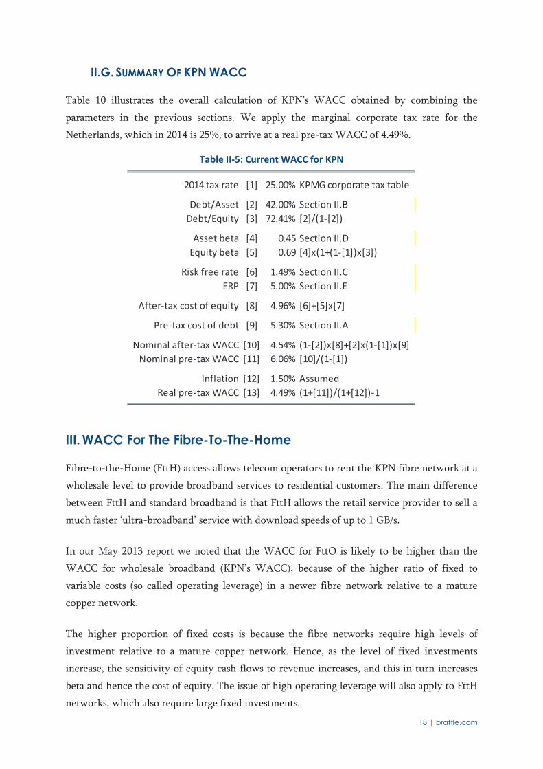
Table 10 illustrates the overall calculation of KPN’s WACC obtained by combining the

parameters in the previous sections. We apply the marginal corporate tax rate for the

Netherlands, which in 2014 is 25%, to arrive at a real pre-tax WACC of 4.49%.

Table II-5: Current WACC for KPN

III. WACC For The Fibre-To-The-Home

Fibre-to-the-Home (FttH) access allows telecom operators to rent the KPN fibre network at a

wholesale level to provide broadband services to residential customers. The main difference

between FttH and standard broadband is that FttH allows the retail service provider to sell a

much faster ‘ultra-broadband’ service with download speeds of up to 1 GB/s.

In our May 2013 report we noted that the WACC for FttO is likely to be higher than the

WACC for wholesale broadband (KPN’s WACC), because of the higher ratio of fixed to

variable costs (so called operating leverage) in a newer fibre network relative to a mature

copper network.

The higher proportion of fixed costs is because the fibre networks require high levels of

investment relative to a mature copper network. Hence, as the level of fixed investments

increase, the sensitivity of equity cash flows to revenue increases, and this in turn increases

beta and hence the cost of equity. The issue of high operating leverage will also apply to FttH

networks, which also require large fixed investments.

2014 tax rate [1] 25.00% KPMG corporate tax table

Debt/Asset [2] 42.00% Section II.B

Debt/Equity [3] 72.41% [2]/(1-[2])

Asset beta [4] 0.45 Section II.D

Equity beta [5] 0.69 [4]x(1+(1-[1])x[3])

Risk free rate [6] 1.49% Section II.C

ERP [7] 5.00% Section II.E

After-tax cost of equity [8] 4.96% [6]+[5]x[7]

Pre-tax cost of debt [9] 5.30% Section II.A

Nominal after-tax WACC [10] 4.54% (1-[2])x[8]+[2]x(1-[1])x[9]

Nominal pre-tax WACC [11] 6.06% [10]/(1-[1])

Inflation [12] 1.50% Assumed

Real pre-tax WACC [13] 4.49% (1+[11])/(1+[12])-1

19 | brattle.com

However, there are reasons to think that FttH may have even higher systematic risk than

FttO, because of the type of area where the network is deployed or rolled out. In a residential

area the network is largely rolled-out on the basis of ‘demand bundling’ and it is referred to as

FttH. For FttO, the network is in many cases built following a specific request received

directly from the business customer willing to receive the ultra-broadband services.

Because the roll-out of FttH networks anticipates the demand for services from residential

customers, whereas FttO is often built following proven demand, FttH could be a more risky

and speculative investment than FttO. In essence, operators invest ‘pre-emptively’ in FttH

based on anticipated demand, but an economic downturn could mean that the demand is not

realized, or materializes more slowly than anticipated. To the extent that the economic

downturn affects all assets in the market, and is therefore systematic, this would raise the beta

of FttH activities relative to FttO.

Hence, the FttH activity may have a higher systematic risk than both wholesale broadband

services provided over a copper network and FttO activity. Because of this potential

difference ACM have asked us to estimate a separate WACC for the FttH activity.

III.A. THE SEARCH FOR AN FTTH PEER GROUP

To calculate a specific WACC for FttH services, we have first investigated if it is possible to

find one or more listed firms that earn the majority of their revenue from FttH activities –

that is a ‘pure play’ FttH operator. If such firms exist, we could then estimate a beta for the

FttH activity directly from their share prices. To find a ‘pure play’ FttH operator – or an

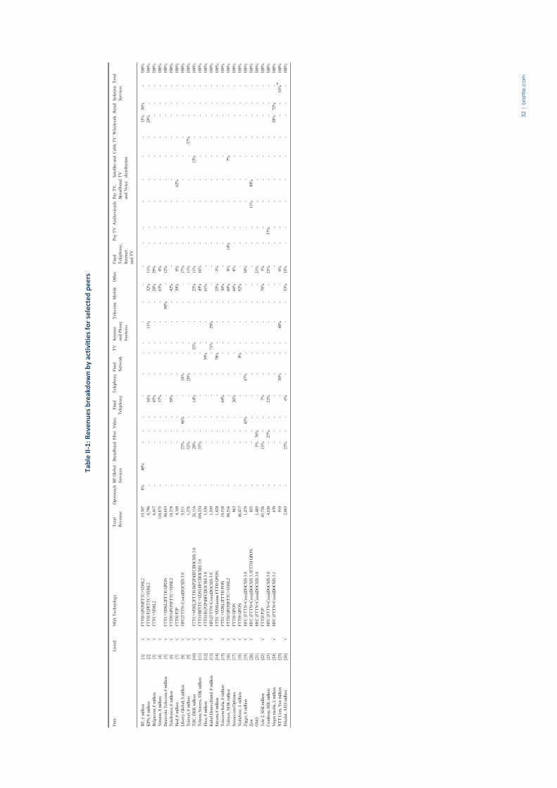
approximation thereof – we have reviewed the annual reports and quarterly presentations of

27 listed telecommunications companies worldwide to find the percentage of revenues and

EBITDA from FttH activities.27 We find that only some companies report the detail of their

FttH revenues, and of these none were a significant percentage of the total. Most companies

did not break out earnings from FttH activity at all. Hence we are not able to identify a pure-

play FttH operator.

This also means that techniques such as ‘beta decomposition’ will not work. Beta

decomposition tries to estimate the beta of a pure-play FttH operator by plotting betas against

the percentage of earnings from FttH. By extrapolating the line, who could in theory estimate

27 We reviewed the 24 companies analysed in our May 2013 report (see Appendix II) and have

expanded our sample to Verizon in USA, Etisalat in United Arab Emirates and NTT in Japan.

20 | brattle.com

the beta of an operator which obtains 100% of their earnings from FttH. However, in reality

there is insufficient data on FttH earnings available. Moreover, given the changing percentage

of FttH earnings over time, and the need to estimate betas over a three-year period, the betas

will not be sufficiently stable to perform this kind of exercise even if earnings data was

available.

The absence of significant revenues from FttH can likely be attributed to the early stage of

deployment of fibre networks, especially in Europe, where a 50% broadband penetration rate

(including both copper and fibre) is envisaged in 2020 accordingly to the European Digital

Agenda.28 This means that even while some companies are investing in fibre networks, their

fibre revenues and profits are very small compared to copper business and mobile activity.

More common ways of identifying revenues in company reports are as fixed-line and mobile,

or by the type of service provided, such as voice, broadband and TV.

As an alternative to finding a peer group from which we can estimate a beta, we have

investigated reasonable ways to modify the KPN’s WACC to make it suitable for the FttH

activity. We discuss possible adjustments below.

III.B. PRECEDENT FROM REGULATORY DECISIONS

According to the European Commission Recommendation on regulated access to Next

Generation Access Networks,29 when setting access prices to the unbundled fibre loop,

National Regulatory Authorities (NRAs) should include a higher risk premium to reflect any

additional and quantifiable investment risk incurred by the incumbent operator.

The European Commission also set out the principles that NRAs should follow in defining the

adequate risk premium. Investment risk should be rewarded by means of a risk premium

incorporated in the cost of capital:30

“NRAs should estimate investment risk inter alia by taking into account the following factors

of uncertainty:

28 Source: Digital Agenda for Europe, Pillar n. IV, “Fast and ultra-fast internet access”, May 2010.

29 Commission Recommendation of 20/09/2010, SEC 1037, par. 4.

30 Commission Recommendation of 20/09/2010, SEC 1037, par. 6.

21 | brattle.com

(i) uncertainty relating to retail and wholesale demand; (ii) uncertainty relating to the costs of

deployment, civil engineering works and managerial execution; (iii) uncertainty relating to

technological progress; (iv) uncertainty relating to market dynamics and the evolving

competitive situation, such as the degree of infrastructure-based and/or cable competition;

and (v) macro-economic uncertainty…

…Criteria such as the existence of economies of scale (especially if the investment is

undertaken in urban areas only), high retail market shares, control of essential

infrastructures, OPEX savings, proceeds from the sale of real estate as well as privileged access

to equity and debt markets are likely to mitigate the risk of NGA investment for the SMP

operator”.

As of today, only France, Spain, Italy and Lithuania have implemented the European

Commission Recommendation on the definition of a WACC premium for FttH services and

defined a premium for fibre services on top of the standard ‘copper WACC’.31 Risk premiums

for FttH are 5.0% in France, 4.81% in Spain and 4.4% in Italy.32 Lithuania does not disclose

the size of the fibre WACC premium it applies.

Values in France and Lithuania seem to have been defined as a pure incentive for fibre

without detailed calculations on the magnitude of systematic risk. However, in Spain and

Italy the NRAs have calculated the risk premium by taking into account the specific risks

identified by the European Commission. Both analyses use a financial model of an FttH

business to estimate the effect of investment risks on FttH profitability.

Specifically, Spain estimates the risk premium as the difference between the Internal Rate of

Return (IRR) of an FttH project and the IRR of less risky ADSL broadband services. The IRR

calculation follows a Montecarlo simulation where the NRA has varied 50,000 times the main

inputs of the project such as: i) cumulative demand of fibre and ADSL services; ii) capital and

31 Note that we have seen reported in some sources that OPTA (now ACM) applies a 3.5% premium

for fibre services. This is not correct – rather, there is a 3.5% ‘headroom’ allowance on the IRR, in

case actual revenues exceed the planned revenues. If the excess return is over 3.5%, then prices

must be reduced.

32 All premiums are expressed in nominal pre-tax terms with the exception of the Italy that considers

real pre-tax values. Risk premium for Italy at 4.4% is calculated by adding the expected inflation

reported by Agcom (1.2%) to the real pre-tax premium of 3.2% (using the Fisher Formula). Source:

Agcom’s consultation 42/15/CONS, table 29 at pag. 129

22 | brattle.com

operating expenditures, iii) market share of incumbent operator, iv) retail prices for fibre and

ADSL services.33

Italy estimates the risk premium by using an approach consistent with the theoretical

framework of the real option. The Italian Regulator built a stylized profitability model for an

investment in FttH and use a Montecarlo simulation to vary three key variables: i) fibre

demand; ii) average revenue per users (ARPU), iii) capital and operating expenditures.

The risk premium rewards two options:

“Wait and see”: an investor in FttH can decide to postpone the investment in order to

have more information (and less risk) on the expected demand, hence obtaining a

higher IRR of the project (according to the assumptions in the model). The increase in

the IRR which results from waiting to invest is the risk premium for FttH;

“Flexibility”: the incumbent is regulated at wholesale level and after the investment is

exposed to the opportunistic behaviours of alternative operators (OLOs). If the real

demand for FttH is lower than expected, OLOs can rely on copper and the incumbent

bears all the risk of the sunk investment. The risk premium also considers that the

incumbent and OLO can share the investment risk, by signing long term contracts.

Hence, the Italian Regulator simulates a trend in the risk premium linked to the

length of the hypothetical long term contract for fibre services, and the percentage of

the costs the OLO pays upfront.

As we noted above the Spain and Italy decisions seem to have considered also some kind of

systematic risk in their calculations. The macroeconomic risks (i.e. GDP, income) in their

analysis can be considered as a proxy of the systematic risk and embedded in the demand

uncertainty of fibre service and the level of the retail price of the service.

However, the Commission’s guidelines is that the risks that the premium is compensating for

include non-systematic risks. That is, it is for risks that an investor could diversify by

investing in many different projects. For example, the risk that a fibre project could

experience cost overruns could be diversified, by investing in a portfolio of projects. The cost

33 Source: CMT Resolución sobre el procedimiento de cálculo de la prima de riesgo en la tasa de

retorno nominal para servicios mayoristas de redes de acceso de nueva generación (MTZ

2012/2155).

23 | brattle.com

of equity should only reflect systematic risk – that is, risks that cannot be diversified – and

that other risks should be accounted for by giving an uplift to the allowed cash flows.34

The ACM allows a 3.5% margin or headroom for KPN, meaning that the realised return can

exceed the expected return by 3.5% without KPN having to reduce its prices. The 3.5%

margin therefore partly compensates KPN for the risk that the return could be less than

expected due to non-systematic risk factors by allowing KPN to keep some of the excess

return when it is higher than expected. Applying the 3.5% margin as well as giving an uplift

to the WACC would result in a ‘double counting’ of the non-systematic risks for KPN.

In this report we are aiming to estimate a WACC for FttH that is directly comparable to

KPN’s WACC, and which covers only systematic risk. In the next section we consider what

effect investment in fibre will have on the systematic risk of a firm.

III.C. FTTH WACC IN THE DCF MODEL

To test whether the FttH WACC premia applied by other NRAs seem reasonable for the

Netherlands, we have used KPN’s DCF model (the DCF model). This is a financial model of

an FttH investment in the Netherlands, and simulates capital investments, the rate of fibre

network build out and take-up, operating costs and revenues for the period 2008 to 2032. By

varying the parameters in the model, we can investigate the effect on the IRR of an FttH

investment, and hence the increase in the WACC that might be required to compensate.

As a starting point we have reviewed the annual reports and quarterly presentations of

incumbent telecoms operators in Spain, Portugal, Italy and France in order to verify if there is

a clear relationship between the macroeconomic conditions – for example GDP and income –

and the demand for FttH post 2008 economic downturn. We could then simulate the effect of

an economic downturn on an FttH investment in the Netherlands, and calculate the effect on

the project’s IRR.

However, we were unable to find evidence of the relationship between the economic crisis

and the take-up of FttH services in annual reports. This is because the operators do not seem

to report their results at this level of detail. The geographic diversification of the operators,

where a significant portion of their earnings comes outside Europe and especially in emerging

34 See for example R.A. Brealey & S.C. Myers, Principles of Corporate Finance, Fifth International

Edition, p. 972. Professor Myers is a Principal of The Brattle Group.

24 | brattle.com

countries in Latin America, as well as the relatively small revenue contribution from FttH

may explain why the operators do not report the outcome of their FttH investments in detail.

Notwithstanding this, as noted above NRAs in Spain and Italy do consider that FttH has a

higher systematic risk than copper broadband or FttC, because systematic changes in

macroeconomic conditions (i.e. GDP, income) will affect the demand for and profitability of

FttH services. Hence, we have used the DCF model to investigate what would need to change

in the model to reduce the IRR by around 4.5 percentage points, this being in the middle of

the range of the FttH premia granted by other NRAs.

We have developed scenarios in the DCF model which reduce the IRR of the FttH

investment by about 4.5 percentage points. The key variable in our simulations is the demand

for FttH services expressed by the ‘adoption rate’ of active customers – that is, the percentage

of customers connected to fibre who actually subscribe to the FttH service. Based on

discussions with the ACM, we consider that the fibre investment program, so both capital and

fixed operating costs – are fixed and would not vary with the adoption rate. Hence, lower

adoption rates reduce the project IRR because costs are fixed while revenues and free cash-

flows from operations are lower than expected.

Figure 6 below illustrates the relationship between the adoption rates and the project IRR in

the DCF model. The trend in the demand of FttH services is the same in all simulations and

the maximum penetration rates are reached in 2027.

25 | brattle.com

Figure 6: Adoption rates and IRR

The base case in the DCF model envisages an adoption rate of 60% from 2027 onwards with a

notional project IRR of 7.85%.35 As illustrated in Figure 6 we find a linear trend, where for

every 5% increase (decrease) in penetration rates the IRR increases (decreases) by around 1%.

Hence to reduce IRR of the FttH investment by around 4.5 percentage points the penetration

rate from 2027 onwards must be 40%, this being 20 percentage points below the base case in

the DCF model. Hence, a reduction in the adoption rate of 20 percentage points decreases the

project IRR from 7.85% (base case) to 3.5%.

A reduction of 20 percentage points of adoption rate may be possible, but it is less clear to

what extent this is a systematic risk – that is, it is a risk associated with the wider market. It

seems intuitive that in an economic downturn consumers may save money by switching to a

35 We understand that 7.85% is not the actual IRR that KPN is expected to earn on its FttH

investments. However, the relationship between the change in the IRR and the change in the

penetration rate – which is what we are interested in measuring in this context – is not sensitive to

the initial IRR. Therefore we are confident that our results would not change significantly if we

started from KPN’s actual expected IRR.

0%

2%

4%

6%

8%

10%

12%

14%

16%

40% 50% 60% 70% 80% 90% 100%

IRR

Un

lev

ere

d C

ash

Flo

ws

%

Penetration %

Source: Brattle calculation on KPN's Model.

Base case in KPN

DCF model

26 | brattle.com

slower internet service, or not taking up the faster FttH service. If economic activity and

incomes are higher consumers may have a higher willingness to spend on FttH services.

Hence the adoption rate will depend in part of wider systematic economic conditions. But a

lower than expected adoption rate could also mean that FttH operators overestimated

consumers’ willingness to pay for a faster FttH service, relative to other slower internet

services. This mis-estimation of demand could occur regardless of economic conditions.

Moreover, we imagine that if adoption rates are consistently lower than expected, the FttH

operator may be able to mitigate the reduction in IRR by reducing or postponing the capital

expenditures after the end of the crisis, or at least focusing on geographic areas with higher

adoption rates.

An alternative scenario is to suppose that the demand of FttH is postponed by about three

years due to the economic downturn, but the maximum penetration rate from 2027 is always

60% as in the base case. Figure 7 reports the comparison between the demand in the base case

and in the alternative scenario.

Figure 7: Active customers (Base case vs postponed take-up)

The scenario of a three year delay due to a crisis seems more clearly consistent with

systematic risk, since the final adoption rate – which depends on inherent consumer

preferences – remains unchanged. Table III-1 shows that a delay in demand reduces the IRR

by 1.87%, or around two percentage points, compared to the base case.

0

500

1000

1500

2000

2500

3000

Act

ive

cu

sto

me

rs "

00

0"

Source: Brattle calculation on KPN's Model.

Penetration

60%

27 | brattle.com

Table III-1: Change in IRR in case of delayed demand

However, we note that this reduction in the IRR only occurs if there is an economic

downturn within the regulatory period. The expected IRR value is actually the weighted

average of the IRR in the case of a delay in demand and the IRR without a delay. For

example, if we assess a reduction in demand scenario as occurring with a 50% probability,

then the expected reduction in the IRR is 50% of 2%, or 1%.

On the other hand, as discussed above we recognise that FttH has higher systematic risks than

FttO. In our May 2013 report we recommended a premium of one percentage point over

copper broadband for FttO. The risks we investigate in this report are over and above the risk

of FttO. This is because FttH shares the same additional risks we identified for FttO, such as

increased operating leverage because of the large investments required, but it has additional

risks over and above the FttO risks. Hence, the 1 percentage point premium that results from

the risk of delayed take up due to an economic crisis should be added onto the 1 percentage

point FttO premium.

Given the analysis above, an FttH premium of two percentage points above the KPN WACC

seems reasonable, and if anything is likely to overestimate the actual systematic risk premia

required if the chance of an economic crisis in the next regulatory period is less than 50%.

However, in our view the consequences of underestimating the risk premium are worse than

the consequences of overestimating it. This is because an underestimation could delay

investment in FttH, thereby delaying the realisation of the EU’s Digital Agenda with the

associated benefits, whereas we understand that KPN does face some pricing constraints – not

last from its own copper broadband service – and may not charge the maximum price possible

in any case.

%

Scenario 60% (Base

Case)

Take-up of 60%

postponed

Notes [A] [B]

IRR Unlevered Cash

Flows [1] 7.85% 5.98%

Change in IRR [2] -1.87%

Notes and Sources:

Brattle calculation on KPN's Model.

Penetration rate

28 | brattle.com

We observe that our estimation is lower than FttH premia recommended by the other NRAs.

However, this is because their premia include both systematic and non-systematic risk while

our exercise is to quantify only the systematic risk related to the FttH activity.

29 | brattle.com

APPENDIX I – Details On KPN’s Leverage

Table appendix I-1: Calculation of Operating Lease Leverage

Operational lease as of 31-Dec-2011 Notes and sources:

Due period [1] < 1 yr 1-5 yrs > 5 yrs

Operational lease €million [2] 457 831 934 p 131, 2011 Annual report of KPN

Years to payment due [3] 1 2 3 4 5 6 7 8 9 10

Projected payments €million [4] 457 207.75 207.75 207.75 207.75 186.8 186.8 186.8 186.8 186.8

[2]. year 1 takes lease amount for

less than 1 year; year 2 to 5 takes

lease amount for 1 to 5 years,

divided by 4; year 6 to 10 takes

lease amount for more than 5 years,

divided by 5.

Averaging period: start [5]

Averaging period: end [6]

Cost of debt [7] 2.12% 2.66% 3.21% 3.69% 4.15% 4.36% 4.57% 4.45% 4.54% 4.59%

Average yields for BBB rated

industrial bonds, denominated in

euros for the period between 01-12-

2011 and 31-12-2011.

Discount factor [8] 97.92% 94.88% 90.95% 86.52% 81.62% 77.41% 73.13% 70.58% 67.08% 63.84% 1/(1+[7])^[3]

Discounted Cash Flows €million [9] 447 197 189 180 170 145 137 132 125 119 [4]x[8]

Present Value of Commitment €million [10] 1,840 Sum [9]



Operational lease €million [12] 527 1029 928 p.142, 2012 Annual report of KPN








divided by 5.



Cost of debt [17] 0.62% 1.05% 1.28% 1.65% 2.05% 2.24% 2.42% 2.60% 2.88% 3.13%




2012 and 31-12-2012.

Discount factor [18] 99.39% 97.94% 96.25% 93.66% 90.35% 87.58% 84.59% 81.44% 77.47% 73.49% 1/(1+[17])^[13]


Present Value of Commitment €million [20] 2,248 Sum [19]



Operational lease €million [22] 203 462 272 p.165, 2013 Annual report of KPN








divided by 5.



Cost of debt [27] 0.74% 0.97% 1.31% 1.71% 2.06% 2.35% 2.63% 2.89% 3.16% 3.47%




2013 and 31-12-2013.

Discount factor [28] 99.27% 98.09% 96.17% 93.44% 90.29% 87.00% 83.38% 79.61% 75.58% 71.12% 1/(1+[27])^[23]


Present Value of Commitment €million [30] 854 Sum [29]



Operational lease €million [32] 171 397 263

page 167, 2014 Annual report of

KPN








divided by 5.



Cost of debt [37] 0.36% 0.49% 0.62% 0.74% 0.89% 1.04% 1.19% 1.33% 1.47% 1.63%




2014 and 31-12-2014.

Discount factor [38] 99.02% 99.02% 98.17% 97.08% 95.68% 93.99% 92.06% 89.99% 87.73% 85.05% 1/(1+[37])^[33]


Present Value of Commitment €million [40] 792 Sum [39]

01/12/2014

31/12/2014

01/12/2011

31/12/2011

01/12/2012

31/12/2012

01/12/2013

31/12/2013

30 | brattle.com

Table appendix I-2: KPN’s Debt and Gearing

Q2 2012 Q3 2012 Q4 2012 Q1 2013 Q2 2013 Q3 2013 Q4 2013 Q1 2014 Q2 2014 Q3 2014 Q4 2014 Q1 2015 2- year 3-year

Share price €/share [1] Bloomberg 7.49 6.79 4.83 3.41 1.90 2.06 2.36 2.63 2.62 2.47 2.53 2.89

Shares outstanding million [2] Bloomberg 1,431.52 1,431.52 1,431.52 1,431.52 4,270.25 4,270.25 4,270.25 4,270.30 4,270.25 4,270.30 4,270.25 4,270.25

Market capitalization €million [3] [1]x[2] 10,718.22 9,722.37 6,918.32 4,888.07 8,122.57 8,817.95 10,064.52 11,248.11 11,168.85 10,536.71 10,810.82 12,358.86

Net debt €million [4] Bloomberg 12,961.00 13,016.00 12,610.00 12,277.00 9,803.00 9,638.00 9,718.00 10,275.00 10,584.00 10,419.00 8,165.00 8,165.00

PV of oprating lease €million [5] See note 2,044.01 2,145.78 2,247.55 1,899.14 1,550.72 1,202.31 853.90 838.53 823.16 807.79 792.42 792.42

Net debt adj. for lease €million [6] [4]+[5] 15,005.01 15,161.78 14,857.55 14,176.14 11,353.72 10,840.31 10,571.90 11,113.53 11,407.16 11,226.79 8,957.42 8,957.42

Enterprise value €million [7] [3]+[6] 25,723.24 24,884.15 21,775.88 19,064.21 19,476.29 19,658.26 20,636.42 22,361.63 22,576.01 21,763.50 19,768.24 21,316.29

Gearing (Debt/Equity) [8] [6]/[3] 140.0% 155.9% 214.8% 290.0% 139.8% 122.9% 105.0% 98.8% 102.1% 106.5% 82.9% 72.5% 103.8% 135.9%

Gearing (Debt/Asset) [9] [8]/(1+[8]) 58.3% 60.9% 68.2% 74.4% 58.3% 55.1% 51.2% 49.7% 50.5% 51.6% 45.3% 42.0% 50.9% 57.6%

Notes and sources:

[5]: Calculated from operating lease reported in various ARs. Split the yearly change equally to derive quarterly values.

Average

31 | brattle.com

APPENDIX II – FttH Peer Group Analysis

32 |

bra

ttle

.co

m

Ta

ble

II-

1:

Re

ve

nu

es

bre

ak

do

wn

by

act

ivit

ies

for

sele

cte

d p

ee

rs

Fir

m

Lis

ted

NG

A T

ech

no

log

yT

ota

l

Rev

enu

e

Op

enre

ach

BT

Glo

bal

Ser

vic

es

Bro

adb

and

Fib

erV

ideo

F

ixed

Tel

eph

on

y

Tel

eph

on

yF

ixed

Net

wo

rk

TV

Inte

rnet

and

Ph

on

e

bu

sin

ess

Tel

eco

ms

Mo

bile

Oth

erF

ixed

Tel

eph

on

y,

Inte

rnet

and

TV

Pay

TV

Au

dio

vis

ual

sP

ay T

V,

Bro

adb

and

and

Vo

ice

Sat

ellit

e an

d

TV

dis

trib

uti

on

Cab

le T

VW

ho

lesa

leR

etai

lS

olu

tio

n

Ser

vic

es

To

tal

BT

, £ m

illio

n[1

]

19,3

078%

40%

--

--

--

--

--

--

--

--

-15

%36

%-

100%

KP

N, €

mill

ion

8,

796

--

--

16%

--

-11

%-

11%

--

--

--

--

100%

Bel

gac

om

, € m

illio

n[3

]6,

417

--

--

43%

--

--

--

--

--

--

--

100%

Ver

izo

n, $

mill

ion

[4]

110,

875

--

--

37%

--

--

-63

%0%

--

--

--

--

-10

0%

[5]

58

,653

--

--

--

--

-88

%-

--

--

--

--

-10

0%

Tel

efo

nic

a, €

mill

ion

[6]

18

,378

--

--

58%

--

--

--

--

--

--

--

-10

0%

Ilia

d, €

mill

ion

[7]

4,16

8-

--

--

--

--

-39

%0%

--

--

--

--

100%

Lib

erty

Glo

bal

, $ m

illio

n[8

]

9,51

1-

-46

%-

14%

--

--

-17

%-

--

--

--

--

100%

Tel

enet

, € m

illio

n[9

]1,

376

--

--

--

--

-11

%-

--

--

37%

--

-10

0%

[10]

-

--

14%

--

15%

--

11%

--

--

15%

--

--

100%

Tel

enia

So

ner

a, S

EK

mill

ion

[11]

10

4,35

4-

35%

--

--

--

--

49%

16%

--

--

--

--

-10

0%

Elis

a, €

mill

ion

1,53

0-

--

--

-39

%-

--

61%

--

--

--

--

--

100%

[13]

1,

599

--

--

--

-71

%-

--

--

--

--

--

-10

0%

Eir

com

, € m

illio

n[1

4]

--

--

--

78%

--

--3

%-

--

--

--

--

100%

Tel

eco

m I

talia

, € m

illio

n[1

5]

19,5

38-

--

-64

%-

--

--

36%

--

--

--

--

--

100%

Tel

eno

r, N

OK

mill

ion

[16]

98

,516

--

--

--

--

--

69%

9%14

%-

--

7%-

--

-10

0%

[17]

FT

TH

GP

ON

863

--

--

--

--

-66

%8%

--

--

--

--

-10

0%

Vo

daf

on

e, £

mill

ion

[18]

FT

TH

GP

ON

46,4

17-

--

--

-8%

--

--

--

--

--

--

-10

0%

Zig

go

, € m

illio

n[1

9]

1,47

8-

--

43%

-47

%-

--

--

10%

--

--

--

--

-10

0%

Zo

n

85

5-

--

--

--

--

--

--

-11

%89

%-

--

--

100%

ON

O

1,48

5-

3%76

%-

--

--

--

--

--

--

--

--

100%

-13

%-

-7%

--

--

-78

%3%

--

--

--

--

-10

0%

Co

mh

em, S

EK

mill

ion

-

--

--

--

--

-37

%-

--

--

--

100%

Vir

gin

med

ia, £

mill

ion

67

0-

--

--

--

--

--

--

--

--

--

100%

NT

T C

om

, Yen

mill

ion

910

--

--

-30

%-

-48

%-

-6%

--

--

--

--

16%

100%

--

-6%

--

--

-53

%15

%-

--

--

--

--

100%

33 |

bra

ttle

.co

m

No

tes

and

So

urc

es:

FT

TH

GP

ON

= F

iber

to

th

e h

om

e

FT

TB

= F

iber

to

th

e b

usi

nes

s

FT

TC

= F

iber

to

th

e ca

bin

et

FT

TN

= F

iber

to

th

e n

od

e o

r n

eig

hb

orh

oo

d

34 |

bra

ttle

.co

m

Ta

ble

II-

2:

EB

ITD

A b

rea

kd

ow

n b

y a

ctiv

itie

s fo

r se

lect

ed

pe

ers

Fir

m

Lis

ted

NG

A T

ech

no

log

yT

ota

l B

road

ban

dF

ixed

Tel

eph

on

y

Wir

elin

eP

ay T

V,

Bro

adb

and

an

d

Vo

ice

Au

do

vis

ual

sM

ob

ility

serv

ice

Op

enre

ach

Wh

ole

sale

Ret

ail

Tel

eph

on

yO

ther

To

tal

BT

, £ m

illio

n[1

]F

TT

H G

PO

N6,

064

--

--

--

38%

30%

-10

0%

KP

N, €

mill

ion

5,13

8-

--

--

--

--

--

0%

Bel

gac

om

, € m

illio

n[3

]1,

897

--

--

--

--

--

-0%

Ver

izo

n, $

mill

ion

[4]

--

--

--

--

--

-0%

[5]

FT

TH

GP

ON

--

--

--

--

--

-0%

Tel

efo

nic

a, €

mill

ion

[6]

FT

TH

GP

ON

-

Ilia

d, €

mill

ion

[7]

--

--

--

--

--

-0%

Lib

erty

Glo

bal

, $ m

illio

n[8

]-

0%

Tel

enet

, € m

illio

n[9

]-

0%

[10]

HF

C

10,4

41-

--

--

--

--

--

0%

Tel

enia

So

ner

a, S

EK

mill

ion

[11]

HF

C

-0%

Elis

a, €

mill

ion

HF

C

506

--

--

--

--

--

-0%

[13]

-16,

568

--

--

--

--

--

-0%

Eir

com

, € m

illio

n[1

4]

som

e F

TT

H G

PO

N

648

--

--

--

--

--

-0%

Tel

eco

m I

talia

, € m

illio

n[1

5]

FT

TH

PO

N

--

--

--

--

--

-0%

Tel

eno

r, N

OK

mill

ion

[16]

FT

TH

GP

ON

--

--

--

--

--

-0%

[17]

FT

TH

GP

ON

--

4%-

-94

%-

--

-10

0%

Vo

daf

on

e, £

mill

ion

[18]

FT

TH

GP

ON

14,4

75-

--

--

--

--

--

0%

Zig

go

, € m

illio

n[1

9]83

5-

--

--

--

--

--

0%

Zo

n

FT

TH

GP

ON

93-

--

84%

--

--

--

16%

100%

ON

O36

7-

--

--

--

--

--

0%

10,9

609%

--

-77

%-

--

-10

0%

Co

mh

em, S

EK

mill

ion

1,77

0-

--

--

--

--

--

0%

Vir

gin

med

ia, £

mill

ion

-0%

35 |

bra

ttle

.co

m

No

tes

and

So

urc

es:

#R

EF

!

FT

TH

GP

ON

= F

iber

to

th

e h

om

e

FT

TB

= F

iber

to

th

e b

usi

nes

s

FT

TC

= F

iber

to

th

e ca

bin

et

FT

TN

= F

iber

to

th

e n

od

e o

r n

eig

hb

orh

oo

d

Th

e to

tal r

even

ues

are

th

e re

ven

ues

gen

erat

ed in

Ho

llan

d w

hic

h a

re t

he

67%

of

the

tota

l co

nso

lidat

ed

h

36 | brattle.com 36 | brattle.com

the waccfor kpn and ftth - autoriteit consument & markt · 2015-07-08 · an ftth network. we...

Documents