three essays on short-term interest rate futures

Louisiana State UniversityLSU Digital Commons

LSU Historical Dissertations and Theses Graduate School

1994

Three Essays on Short-Term Interest Rate Futures.Yiuman TseLouisiana State University and Agricultural & Mechanical College

Follow this and additional works at: https://digitalcommons.lsu.edu/gradschool_disstheses

This Dissertation is brought to you for free and open access by the Graduate School at LSU Digital Commons. It has been accepted for inclusion inLSU Historical Dissertations and Theses by an authorized administrator of LSU Digital Commons. For more information, please [email protected].

Recommended CitationTse, Yiuman, "Three Essays on Short-Term Interest Rate Futures." (1994). LSU Historical Dissertations and Theses. 5837.https://digitalcommons.lsu.edu/gradschool_disstheses/5837

https://digitalcommons.lsu.edu?utm_source=digitalcommons.lsu.edu%2Fgradschool_disstheses%2F5837&utm_medium=PDF&utm_campaign=PDFCoverPages

https://digitalcommons.lsu.edu/gradschool_disstheses?utm_source=digitalcommons.lsu.edu%2Fgradschool_disstheses%2F5837&utm_medium=PDF&utm_campaign=PDFCoverPages

https://digitalcommons.lsu.edu/gradschool?utm_source=digitalcommons.lsu.edu%2Fgradschool_disstheses%2F5837&utm_medium=PDF&utm_campaign=PDFCoverPages

https://digitalcommons.lsu.edu/gradschool_disstheses?utm_source=digitalcommons.lsu.edu%2Fgradschool_disstheses%2F5837&utm_medium=PDF&utm_campaign=PDFCoverPages

https://digitalcommons.lsu.edu/gradschool_disstheses/5837?utm_source=digitalcommons.lsu.edu%2Fgradschool_disstheses%2F5837&utm_medium=PDF&utm_campaign=PDFCoverPages

mailto:[email protected]

INFORMATION TO USERS

This manuscript has been reproduced from the microfilm master. UMI films the text directly from the original or copy submitted. Thus, some thesis and dissertation copies are in typewriter face, while others may be from any type of computer printer.

The quality of this reproduction is dependent upon the quality of the copy submitted. Broken or indistinct print, colored or poor quality illustrations and photographs, print bleedthrough, substandard margins, and improper alignment can adversely affect reproduction.

In the unlikely event that the author did not send UMI a complete manuscript and there are missing pages, these will be noted. Also, if unauthorized copyright material had to be removed, a note will indicate the deletion.

Oversize materials (e.g., maps, drawings, charts) are reproduced by sectioning the original, beginning at the upper left-hand corner and continuing from left to right in equal sections with small overlaps. Each original is also photographed in one exposure and is included in reduced form at the back of the book.

Photographs included in the original manuscript have been reproduced xerographically in this copy. Higher quality 6" x 9" black and white photographic prints are available for any photographs or illustrations appearing in this copy for an additional charge. Contact UMI directly to order.

University Microfilms International A Bell & Howell Information C om p any

3 0 0 North Z e eb Road. Ann Arbor, Ml 4 8 1 0 6 -1 3 4 6 USA 3 1 3 /7 6 1 -4 7 0 0 8 0 0 /5 2 1 -0 6 0 0

O rder N u m b er 9508610

Three essays on short-term interest rate futures

Tse, Yiuman, Ph.D.The Louisiana State University and Agricultural and Mechanical Col., 1994

UMI300 N. ZeebRd.Ann Arbor, MI 48106

THREE ESSAYS ON SHORT-TERM INTEREST RATE FUTURES

A DissertationSubmitted to the Graduate Faculty of the

Louisiana State University and Agricultural and Mechanical College

in partial fulfillment of the requirements for the degree of

Doctor of Philosophy

in theInterdepartmental Program in Business Administration

byYiuman Tse

B.S.(Mech. Eng.)/ University of Hong Kong, 1986 M.B.A., SUNY at Binghamton, 1989

August 1994

ACKNOWLEDGEMENTS

I wish to express my sincere appreciation to Professor G. Geoffrey Booth, my committee chairman, without whose guidance and inspirations this dissertation would not have been completed. I also wish to thank the other members of my committee, Professors William Lane, Dr. Tae-Hwy Lee, Dr. Gary Sanger, and Dr. Myron Slovin, for their valuable insights and helpful comments throughout this dissertation. I am grateful to Professor Ram Sriram for his presence on my committee. I am also indebted to Professors Carter Hill and Faik Koray for their enlightenment.

My most heartfelt gratitude and adoration go to my wife, Mandy, whose love and understanding are always evident. Finally, I dedicate this dissertation to my parents for their constant support and encouragement.

ii

TABLE OF CONTENTS

PageACKNOWLEDGEMENTS iiABSTRACT V

CHAPTER 1: INTRODUCTION1.1 Overview 11.2 Lead/Lag Relationships between TB 2

and ED Futures1.3 Volatility Spillover between TB and ED 31.4 International Transmission of Information 4

in Eurodollar Futures Markets1.5 Cointegration and Fractional Cointegration 5

Tests with Conditional Heteroskedasticity1.6 Summary 7

CHAPTER 2: THE RELATIONSHIP BETWEEN U.S. AND EURODOLLAR INTEREST RATES:EVIDENCE FROM THE FUTURES MARKETS

2.1 Introduction 82.2 Review of Literature 112.3 Data and Preliminary Statistics 142.4 Cointegration Analysis 242.5 Error Correction Model and Granger Causality 412.6 Contemporaneous Relationships and 54

Simultaneous Equations Models2.7 Fractional Cointegration 602.8 Conclusions 70

CHAPTER 3: COMMON VOLATILITY AND VOLATILITY SPILLOVERBETWEEN U.S. AND EURODOLLAR INTEREST RATES: EVIDENCE FROM THE FUTURES MARKETS

3.1 Introduction 733.2 Data and Preliminary Statistics 753.3 Common Volatility 803.4 TED Spread and Volatility Spillovers 823.5 Conclusions 95

iii

97100104108112117124137139143

154160166182187

THE INTERNATIONAL TRANSMISSION OF INFORMATION IN EURODOLLAR FUTURES MARKETS

IntroductionData and Summary Statistics Volatility During Trading and Nontrading

HoursUnit Root and Cointegration Granger Causality among Markets Variance Decomposition and Impulse Response

AnalysisVolatility Transmission and Spillover ConclusionsSUMMARY AND CONCLUSIONS

COINTEGRATION AND FRACTIONAL COINTEGRATION TESTS WITH CONDITIONAL HETEROSKEDASTICITY: A MONTE CARLO INVESTIGATION

Introduction The Simulation Design Results of the Simulation Conclusions

iv

ABSTRACT

This dissertation examines the relationship between U.S. and Eurodollar interest rates by using daily U.S. Treasury bill and Eurodollar futures. Weak evidence of cointegration is found. The VAR and error correction models do not give better forecast performance than the naive model. Other evidence, particularly the simultaneous equations model, suggests that the hypothesis of contemporaneous relationships is not rejected. Further analysis of the deviations from the cointegrating relationship shows that the Treasury bill and Eurodollar futures are fractionally cointegrated after the 1987 stock market crash. Some preliminary statistics seem to support the hypothesis that these futures interest rates share the same volatility process, which follow a GARCH process. However, this hypothesis is rejected by the common volatility test. A bivariate EGARCH model which allows for asymmetric volatility influence of the TED spread, as well as that of the domestic market, is used to analyze the volatility spillovers between markets. Results show that the lagged TED spread change is the driving force of the volatility process.

This dissertation also studies the international transmission of identical Eurodollar futures contracts traded on three exchanges, the IMM, SIMEX, and LIFFE. An approach of variance decomposition and impulse response functions exploring the common factor in the cointegration system is employed. It is shown that the markets are extremely efficient

on a daily basis such that each market, when it is trading, impounds all the information that will affect other markets, and rides on the common stochastic trend. The significant results of volatility spillovers among markets suggest that certain market dynamics lead to a continuation of volatility. Particularly, the volatility spillover mechanism may be influenced by the U.S. stock markets.

In addition, using a Monte Carlo approach, this dissertation investigates whether the cointegration and fractional cointegration results reported are biased by the GARCH innovations. The size of fractional cointegration tests is evinced to be less distorted by the GARCH effects.

CHAPTER 1

INTRODUCTION

1.1 Overview

Knowledge of the causal relationship between interest rate changes in the domestic and external markets is of major importance to the understanding of international financial integration. Previous studies, however, have presented conflicting evidence concerning the relative speeds of interest rate adjustment to new information in external and domestic money markets. Conflicting conclusions among previous studies may be attributed to the differences in the time periods examined, the data used, and the empirical techniques employed. Nevertheless, any lead/lag relationships between close substitutes reported, except Kaen, Helms, and Booth (1983) , who use futures data, imply transaction costs, market imperfections, and/or time-varying risk premia. To minimize these effects on the analysis of the adjustment processes, daily 3-month U.S. Treasury bill and Eurodollar futures contracts, TB and ED hereafter, are used in the current study. Moreover, as the yield on a Treasury bill or Eurodollar futures reflects the market's assessment about spot interest rate level in the future, yields implied by the futures may provide a more accurate interpretation of the adjustment process.

1

2

Eurodollar futures are now the most actively traded short-term interest rate futures contract. The Eurodollar futures market is designed specifically for the international market with much of the activity from sources external to the United States. Eurodollar futures are used primarily by large banks and multinational corporations desiring to avoid the interest rate risk in international financial transactions. Moreover, Eurodollar futures contracts are actively traded at the IMM in Chicago, at LIFFE in London, and at the Singapore. A better understanding of the information transmission mechanism among these Eurodollar futures markets may provide investors with more efficient strategies for hedging or speculating interest rate risk particularly with Eurodollar deposits.

1.2 Lead/Lag Relationships between TB and ED Futures

Chapter 2 examines the lead/lag relationship in the Granger-cause sense between U.S. and Eurodollar interest rates in futures contracts. It shows weak evidence of cointegration between yields on U.S. Treasury bill and Eurodollar futures for the period March 1982 - February 1993. Specifically, the cointegration results are sensitive to the different cointegration tests used, and are likely to be biased by the conditional heteroskedasticity in the series. The VAR and error correction models do not give better forecast performance than the naive model. Other evidence given in the

chapter, particularly the simultaneous equations model, suggests that the hypothesis of contemporaneous relationships, at least on daily basis, is not rejected. Further analysis of the deviations from the cointegrating relationship shows that the Treasury bill and Eurodollar futures are fractionally cointegrated after the 1987 stock market crash. That is, the deviations from the cointegrating relationship are shown to possess long memory and be well modeled as fractionally integrated 1(d) process, where d is in the range of zero and one. Particularly, the equilibrium errors between markets exhibit slow mean reversion.

1.3 Volatility Spillover between TB and ED

All previous research investigates the relationship between U.S. and Eurodollar interest rates via the first moment of the time series. Ross (1989), however, shows that the variance of price changes is related directly to the rate of flow of information. Hence, previous studies ignoring the volatility mechanism may not offer a thorough understanding of the information transmission process. In Chapter 3, Treasury bill and Eurodollar futures are employed to investigate the volatility spillovers between U.S. and Eurodollar interest rates.

Both TB and ED exhibit the volatility clustering phenomenon, and the GARCH-type model of Engle (1982) and Bollerslev (1986) is shown to provide a good fit for them.

Some preliminary statistics seem to support the hypothesis that TB and ED share the same volatility process, which follows a GARCH process. However, this hypothesis is rejected by the common volatility test of Engle and Kozicki (1993).

Chapter 2 documents that the TED spread (ED minus TB yields) reflects the soundness of the international financial markets. In general, events that jeopardize the economy, especially the soundness of the banking system, tend to widen the spread. A highly volatile TED spread indicates a state of uncertainty; accordingly, if the spread changes substantially on a particular day, TB and ED will also change in either direction in the following day. A bivariate EGARCH model which allows for asymmetric volatility influence of the TED spread, as well as that of the domestic market, is used to analyze the volatility spillovers between markets. Results show that the lagged TED spread change is the driving force of the volatility spillover mechanism.

1.4 International Transmission of Information in Eurodollar Futures Markets

Chapter 4 studies the international transmission of identical Eurodollar futures contracts traded on three exchanges, the IMM, SIMEX, and LIFFE. It first examines the volatility of interest rate changes in each market during trading and non-trading hours. The U.S. market gives the greatest trading to non-trading time variance ratio; the

Singapore market, in contrast to the other two markets, gives a higher non-trading time variance than trading time variance. These results are consistent with the fact that Eurodollar interest rates are driven by the economic news concerning the U.S. and European countries. Second, the interest rates of the three markets are shown to be cointegrated with a single common stochastic trend. An approach of variance decomposition and impulse response functions exploring the common factor in the cointegration system is employed. Having recognized the nonsynchronous trading problem among these three markets, it is shown that the common factor is simply driven by the market that is placed in the last order (within 24 hours) in the vector error correction model. Specifically, each market, when it is trading, impounds all the information that will affect other markets, and rides on the common stochastic trend. Third, intra-daily (open and closing) volatility spillovers are strongly suggested. Moreover, results show that the U.S. stock markets play an important role in the volatility spillover mechanism among Eurodollar futures markets.

1.5 Cointegration and Fractional Cointegration Tests with Conditional Heteroskedasticity

Despite the extensive literature on autoregressive conditional heteroskedasticity (ARCH) of Engle (1982), generalized ARCH (GARCH) of Bollerslev (1986), and related models, relatively little attention has been given to the

issue of the GARCH effects on the performance of cointegration and fractional cointegration tests. The Appendix of this dissertation examines this issue by using a Monte Carlo approach. This studies whether the cointegration and fractional cointegration results reported in Chapters 2 and 4 are biased by the GARCH errors.

Firstly, it analyzes the finite sample performance of Johansen's (1988) likelihood ratio tests for cointegration, and comparisons are concluded with other cointegration tests. The cointegration tests tend to over-reject the null hypothesis of no cointegration in favor of finding cointegration too often in the presence of GARCH errors, but the bias is not very serious except when the variance processes are nearly degenerate and integrated. In general, the Johansen trace test is found to have smaller size distortion than the Johansen maximum eigenvalue test. The Dickey-Fuller test with the White (1980) heteroskedasticity correction may improve the size of the test but has a very poor power performance.

Secondly, it analyzes the GARCH effects on fractional integration tests of Geweke-Porter-Hudak (GPH) and modified rescaled range (MRR) for the analysis of the deviations from the cointegrating relationship. The fractional integrated error correction term suggests long run memory of the relationship. Results show that the size distortion problem is less serious for fractional cointegration tests.

71.6 Summary

The next two chapters examine the relationship between U.S. Treasury bill and Eurodollar futures: Chapter 2 analyzes the lead/lag and (fractional) cointegration relationship; Chapter 3 investigates the common volatility process and volatility spillovers. These two chapters provide knowledge of the causal relationship and information transmission mechanism between interest rate changes in the domestic and external markets. Chapter 4 focuses on the international transmission process of Eurodollar futures. Using Monte Carlo approach, the Appendix studies whether the cointegration and fractional cointegration results reported in Chapters 2 and 4 are biased by the GARCH innovation.

CHAPTER 2

THE RELATIONSHIP BETWEEN U.S. AND EURODOLLAR INTEREST RATES:

EVIDENCE FROM THE FUTURES MARKETS

2.1 Introduction

This chapter analyzes the relative speeds at which Eurodollar (external) and U.S. (domestic) interest rates in futures contracts incorporate information. The primary question the chapter addresses is whether Eurodollar and U.S. interest rate changes lead/lag one another in the Granger- cause sense, or move contemporaneously.

Knowledge of the causal relationship between interest rate changes in the domestic and external markets is of major importance to the understanding of international financial market integration. One aspect of concern has been the influence of domestic dollar denominated asset returns on comparable external dollar returns. Previous studies, however, have presented conflicting evidence concerning the relative speeds of interest rate adjustment to new information by external and domestic money markets. Earlier studies of Hendershott (1967) and Kwack (1971) support an adjustment process that runs from the domestic money market to the Eurodollar market; Giddy, Dufey, and Min (1979) , in contrast, document a reverse adjustment process. Moreover, Kaen and Hachey (1983) show evidence of a periodic feedback process,

9and Kaen, Halems, and Booth (1983) report a contemporaneous relationship (i.e. no lead/lag relationship). Lately, Fung and Isberg (1992) find that the unidirectional causality leading from the domestic to the external markets for the period of 1981-1983 is reversed for the more recent period of 1984-1988. In sum, all of these studies, except Kaen, Halems, and Booth (1983) who use U.S. Treasury bill and Eurodollar futures prices, report that internal and external interest rates do not adjust at the same speed to new information.

This chapter also uses daily prices of Treasury bill and Eurodollar futures by rolling over nearby contracts during the period March 1982 to February 1994. As pointed out by Kaen, Helms, and Booth (1983), since both are traded on the Chicago Mercantile Exchange (CME), biases due to nonsynchronous data and/or different institutional characteristics of various markets are eliminated. Moreover, examining the relationship between these two short-term interest rate futures illustrates investors' views about Eurodollar deposits' risk premium over Treasury bills. Specifically, trading the interest rate differential between Eurodollar and Treasury bill futures, i.e., the TED spread, can be a means to speculate on general economic conditions and on the soundness of banks in particular without incurring interest rate risk. In general, events that jeopardize the soundness of the banking system tend to widen the spread.

Mixed results of cointegration are given by different cointegration tests, the augmented Dickey-Fuller (ADF), Phillips Z, and Johansen tests, all of which are likely to be biased by the conditional heteroskedasticity effects. In particular, the cointegration tests employed in the chapter tend to reject the null hypothesis of no cointegration even when the series are not cointegrated. Granger-causality tests of the (unrestricted) vector autoregression (VAR) and error correction models (ECM) generally indicate no causality in either direction. Moreover, the improvement in forecasts using the and VAR model and ECM is negligible. The simultaneous equations model further suggests contemporaneous relationships. Nevertheless, the GPH test that is robust to variance nonstationarity gives fairly strong evidence of fractional cointegration for the post-1987 stock crash period. Hence, the deviations from the cointegrating relationship possess long memory and are well modeled as fractionally integrated 1(d) process, where d is in the range of zero and one.

The organization of the chapter is as follows. The next section provides a literature review. Section 2.3 describes the data and preliminary statistics. The main results are given in Section 2.4 where the cointegration, error correction models, Granger causality, and forecasting performance are analyzed. Section 2.5 discusses the simultaneous equations models. Section 2.6 offers a further understanding of the

1 1

relationship by employing the fractional integration and fractional cointegration analysis. The final section concludes the chapter.

2.2 Review of Literature

Early studies of the period between the late 1960s and early 1970s find that the U.S. interest rate markets are relatively isolated from the influence of foreign markets. Hendershott (1967), using a stock adjustment model and the U.S. Treasury bill, concludes that it takes about one year for the Eurodollar rate to completely adjust to changes in the U.S. bill rate. Kwack (1971) extends Hendershott's tests by incorporating foreign interest rates into the analysis; his results support those of Hendershott. However, these results may be explained by the fact that during the period examined, U.S. capital controls and a par value international monetary regime were in place. Moreover, the Eurodollar markets were still in their infancy with respect to the numbers and variety of market participants.

In the post-U.S. capital control era, Giddy, Dufrey, and Min (1979) propose the substitution of a deposit rate and examine the behavior of the interest differential between bank lending and deposit rates. They find that Eurodollar rates respond more efficiently to information, hence causality runs from the external to the domestic market. Giddy, Dufrey, and Min (1979) attribute this non-contemporaneous behavior to the

1 2

fact that the Eurocurrency markets are more competitive with regard to the participant market power than are the domestic markets.

In some more recent papers (e.g., Kaen and Hachey, 1983; Swanson, 1988) , while the main direction of causality is shown to run from the external to the domestic markets, a feedback process is frequently observed. However, Kaen, Halms, and Booth (1983), using 3-month Treasury bill and Eurodollar futures contracts, conclude that the interest rate changes exhibit contemporaneous behavior, consistent with semi-strong form efficiency. To be more specific, past information about price changes in the domestic market does not provide information about current price changes for the external market and vice versa. The statistical technique used in these papers is the Granger-Sims causality test, which tests whether the past, present and future information associated with a particular variable helps to improve forecasts of a second variable (Granger, 1969; Sims, 1972).

However, it is now well known that if two nonstationary variables are cointegrated, a vector autoregression in the first difference, which is used in the previous Granger causality tests, is misspecified (Engle and Granger, 1987). Fung and Isberg (1992) recently find that U.S. and Eurodollar certificate of deposit rates are cointegrated, and they examine the causal relationship by using an error correction model. Their results show that there is a structural change in

13the interest rates. In the 1981-1984 period, there exists unidirectional causality leading from the domestic to the external markets. But, in the more recent 1984-1988 period, significant reverse causality is observed. They argue that this change may be due to the increased size of the Eurocurrency market and to more rapid movements toward deregulation in the European as compared to the U.S. markets.

Conflicting conclusions among previous studies may be attributed to the differences in the time periods examined, the data used, and the empirical techniques employed. Nevertheless, any lead/lag relationships between close substitutes reported, except Kaen, Halms, and Booth (1983), imply transaction costs, market imperfections, and/or time- varying risk premia. To minimize these effects on the analysis of the adjustment process, daily 3-month U.S. Treasury bill and Eurodollar futures contracts are used in the current study. Moreover, as the yield on a T-bill or Eurodollar futures reflects the market's assessment about spot interest rate levels in the future, yields implied by the futures may provide a more accurate interpretation of the adjustment process.

Since Kaen, Helms, and Booth (1983) use only the three earliest individual contracts of Eurodollar futures traded in 1981-1992, an updated examination is required. This chapter rolls over the nearby futures contracts of the past six years, and mitigates the bias due to two phenomena related to

14liquidity. First, the daily trading volume is small (or no trading) during the early trading period (more than six months) of each individual contract. Second, during the several days before its delivery date, volume and open interest tend to rise and then fall sharply, as traders exit the market to avoid having to make or take delivery.

2.3 Data and Preliminary Statistics

2.3.1 Data EnvironmentThe 3-month U.S. Treasury bill and Eurodollar futures are

traded at the International Monetary Market (IMM), a division of the Chicago Mercantile Exchange.1 Daily closing and open prices from March 1, 1982 to February 22, 1994 (3032observations) are collected from Commodity Systems, Inc. (CSI). This covers the whole trading history of Eurodollar futures.2 Both prices are quoted on an index basis at 2:00 PM Chicago time. The problem of nonsynchronous trading, therefore, does not appear.

Eurodollar futures contracts with virtually identical specifications are also traded at London International Financial Futures Exchange (LIFFE), and Singapore International Monetary Exchange (SIMEX). Moreover, Eurodollar futures positions that were established at IMM may be offset at SIMEX, and vice versa. Nevertheless, the trading volume at IMM is 10 times more than LIFFE and SIMEX. Chapter 4 examines the international transmission of Eurodollar futures markets.

Eurodollar futures are introduced in December 1981. The first three trading months are not used for any potential problems of an infant market.

15A U.S. Treasury bill futures contract calls for physical

delivery of a 3-month, $1 million, U.S. Treasury bill; a Eurodollar futures contract calls for the delivery (cash settlement) of a $1 million, 3-month, Eurodollar time deposit. The 3-month Eurodollar futures contract is at present the most widely traded short-term interest rate futures contract, and spread trading between these two futures has become increasingly popular. (See Siegel and Siegel (1989, Ch.5), Kolb (1991, Ch.8), and Edwards and Ma (1992, Ch.12) for more information.) Hereafter, for simplicity, the ticker symbols TB and ED are used to represent the 3-month U.S. Treasury bill and Eurodollar futures, respectively.

Unlike Treasury bills, which are sold on discount, Eurodollar time deposits pay add-on interest. To compare them on an equal basis and get a more accurate analysis of the TED spread, the ED yield minus the TB yield, the implied discount yield of TB futures and the implied add-on yield of ED futures are converted into the bond equivalent yield.3 This yield is used from the contract with the nearest delivery month, which

3 The following formulae convert (a) a discount yield; and (b) an add-on yield to a bond equivalent yield respectively: bond equivalent yield =(a)365 x yield/[360 -(yield x days to maturity)];(b)365/360 x yield,where yield = (100 - index price)/100.Nevertheless, results presented through the paper are qualitatively the same when discount yield of TB and add-on yield of ED or the logarithm of dollar futures price is used. This latter observation is especially important since interest rates cannot take on large negative values but the logarithm of prices can.

16is highly liquid, until the first trading day of the delivery month, when it is rolled to the next nearest-to-deliver contract. Yield changes (first differences) are taken before linking the contracts together.4

2.3.2 Preliminary StatisticsSeveral studies find that the October 1987 stock crash

(the crash) changed the structure of international movements between financial markets (see e.g., Malliaris and Urrutia (1992), and Arshanapalli and Doukas (1992)). In fact, both TB and ED experienced the greatest (absolute) percentage yield changes on October 19, 1987 for the period examined. In this chapter, results of the whole period, and both of the pre- (3/1/82 - 9/30/87, 1414 observations) and post-crash (1/4/88 - 6/30/93, 1390 observations) periods are analyzed. The last

seven months (7/1/93 - 2/22/94, 155 observations) are reserved for forecasting. Furthermore, to ensure that the interpretation of test statistics is not distorted by the large sample size used in this chapter, the significance level adopted is 1%, instead of 5%, unless specified. Connolly (1989) provides a detailed explanation on this issue by eliciting the Lindley Paradox. As Connolly points out, the significant level should be adjusted downward with increases

4If this procedure is not employed, some outliers are artificially created on the rollover dates, e.g., 6/1/89, and accordingly, the VAR and ECM models are distorted. See Ma, Jeffrey, and Mattew (1992) for more details on the issue of rolling futures contracts.

17in sample size. Otherwise, spurious significant results are incurred by large sample size distortion.

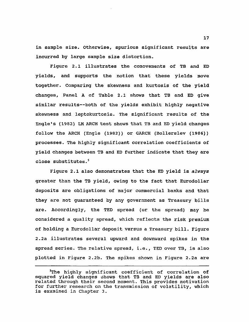
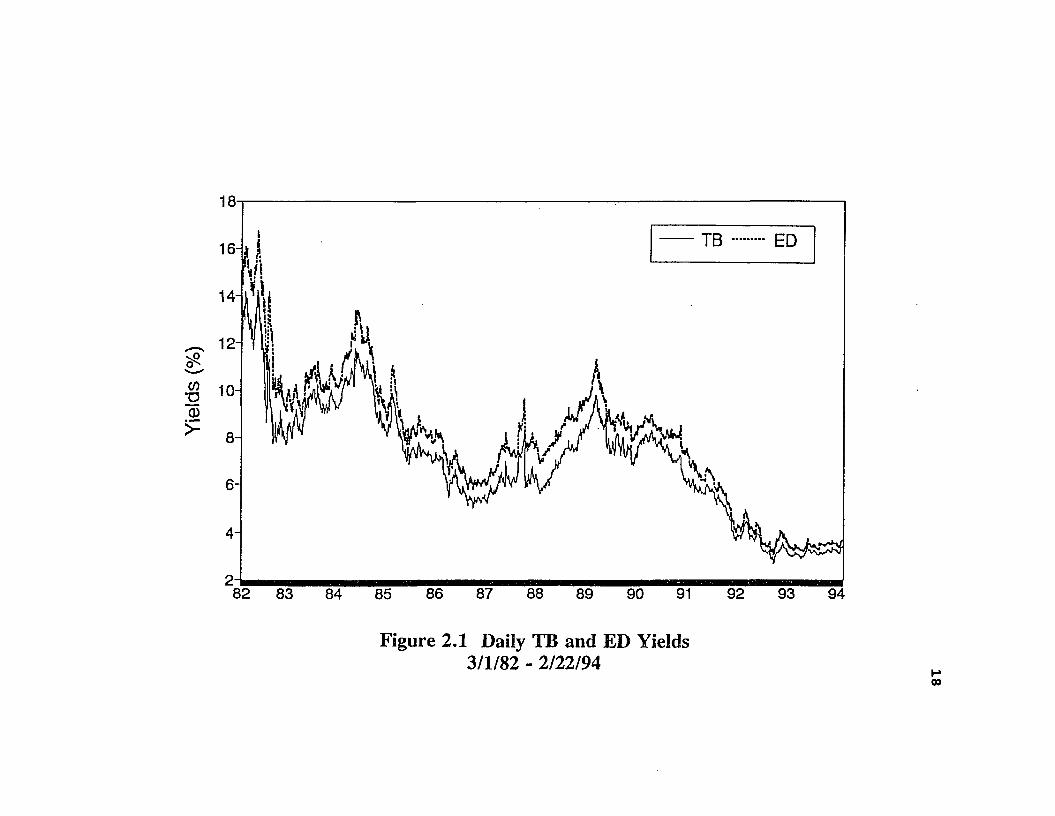
Figure 2.1 illustrates the comovements of TB and ED yields, and supports the notion that these yields move together. Comparing the skewness and kurtosis of the yield changes, Panel A of Table 2.1 shows that TB and ED give similar results— both of the yields exhibit highly negative skewness and leptokurtosis. The significant results of the Engle's (1982) LM ARCH test shows that TB and ED yield changes follow the ARCH (Engle (1982)) or GARCH (Bollerslev (1986)) processes. The highly significant correlation coefficients of yield changes between TB and ED further indicate that they are close substitutes.5

Figure 2.1 also demonstrates that the ED yield is always greater than the TB yield, owing to the fact that Eurodollar deposits are obligations of major commercial banks and that they are not guaranteed by any government as Treasury bills are. Accordingly, the TED spread (or the spread) may be considered a guality spread, which reflects the risk premium of holding a Eurodollar deposit versus a Treasury bill. Figure 2.2a illustrates several upward and downward spikes in the spread series. The relative spread, i.e., TED over TB, is also plotted in Figure 2.2b. The spikes shown in Figure 2.2a are

5The highly significant coefficient of correlation of squared yield changes shows that TB and ED yields are also related through their second moment. This provides motivation for further research on the transmission of volatility, which is examined in Chapter 3.

Yield

s (%

)18

TB ED16-

14-

12-

10-

282 83 8786 88 90 92 93 9484 85 89

Figure 2.1 Daily TB and ED Yields 3/1/82 - 2/22/94

00

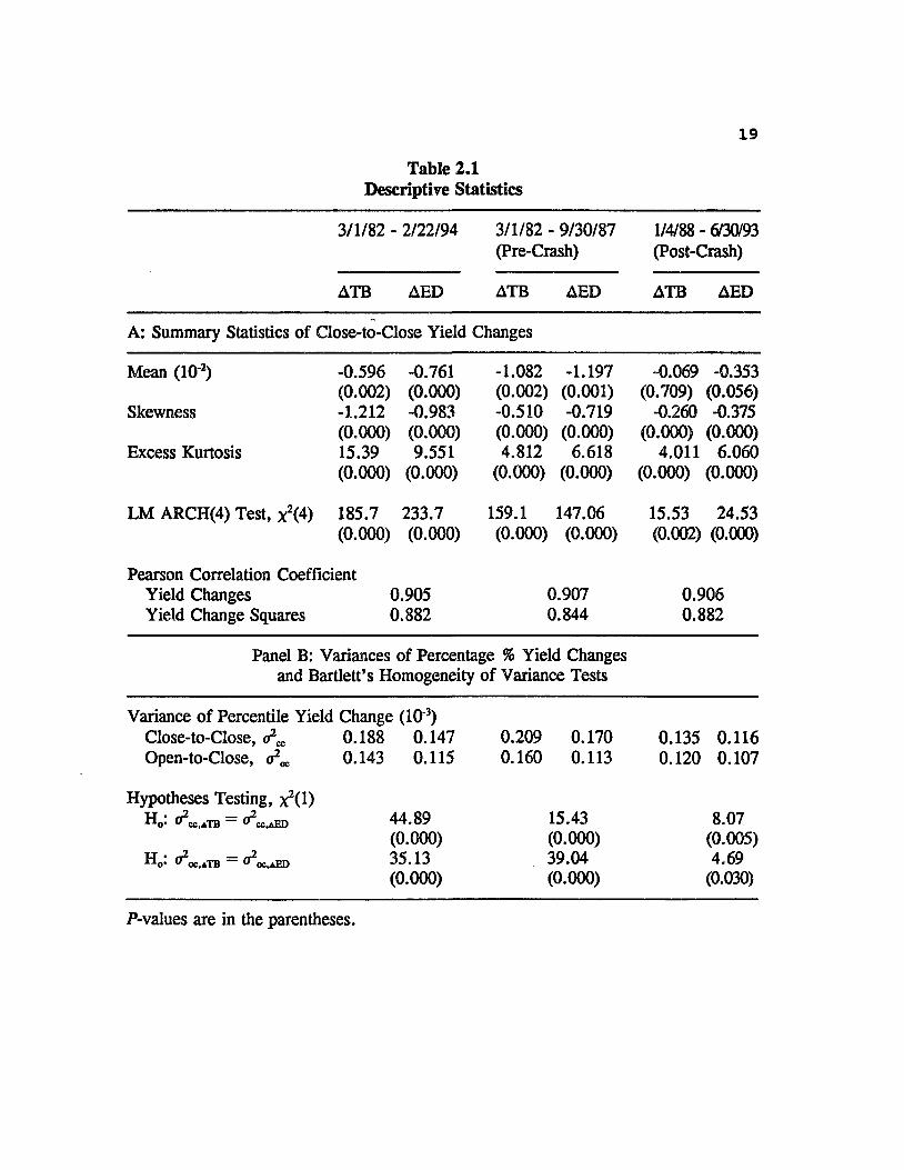
Table 2.1 Descriptive Statistics

19

3/1/82 - 2/22/94 3/1/82 - 9/30/87 (Pre-Crash)

1/4/88 - 6/30/93 (Post-Crash)

ATB AED ATB AED ATB AED

A: Summary Statistics of Close-to-Close Yield Changes

Mean (10 2) -0.596 -0.761 -1.082 -1.197 -0.069 -0.353(0.002) (0.000) (0.002) (0.001) (0.709) (0.056)

Skewness -1.212 -0.983 -0.510 -0.719 -0.260 -0.375(0.000) (0.000) (0.000) (0.000) (0.000) (0.000)

Excess Kurtosis 15.39 9.551 4.812 6.618 4.011 6.060(0.000) (0.000) (0.000) (0.000) (0.000) (0.000)

LM ARCH(4) Test, x2(4) 185.7 233.7 159.1 147.06 15.53 24.53(0.000) (0.000) (0.000) (0.000) (0.002) (0.000)

Pearson Correlation CoefficientYield Changes 0.905 0.907 0.906Yield Change Squares 0.882 0.844 0.882

Panel B: Variances of Percentage % Yield Changesand Bartlett’s Homogeneity of Variance Tests

Variance of Percentile Yield Change (10‘3)Close-to-Close, cr2 0.188 0.147 0.209 0.170 0.135 0.116Open-to-Close, 0.143 0.115 0.160 0.113 0.120 0.107

Hypotheses Testing, ^ (l)H0. U cc,*TB ^cc.aED 44.89 15.43 8.07

(0.000) (0.000) (0.005)Ho: O2oc,*TB = ff2oc,AED 35.13 39.04 4.69

(0.000) (0.000) (0.030)

P-values are in the parentheses.

TED

Spre

ad

and

Spre

ad

Cha

nge TED Spread Spread Change

lyMi

-0.5H82 83 84 85 86 87 88 89 90 91 92 93 94

Figure 2.2a TED Spread and Spread Changetoo

0.4

0.35-

0.3-

0.25-

0.2-

0.15-

0.1-

0.05 8882 83

Figure 2.2b Relative TED Spread (TED/TB)

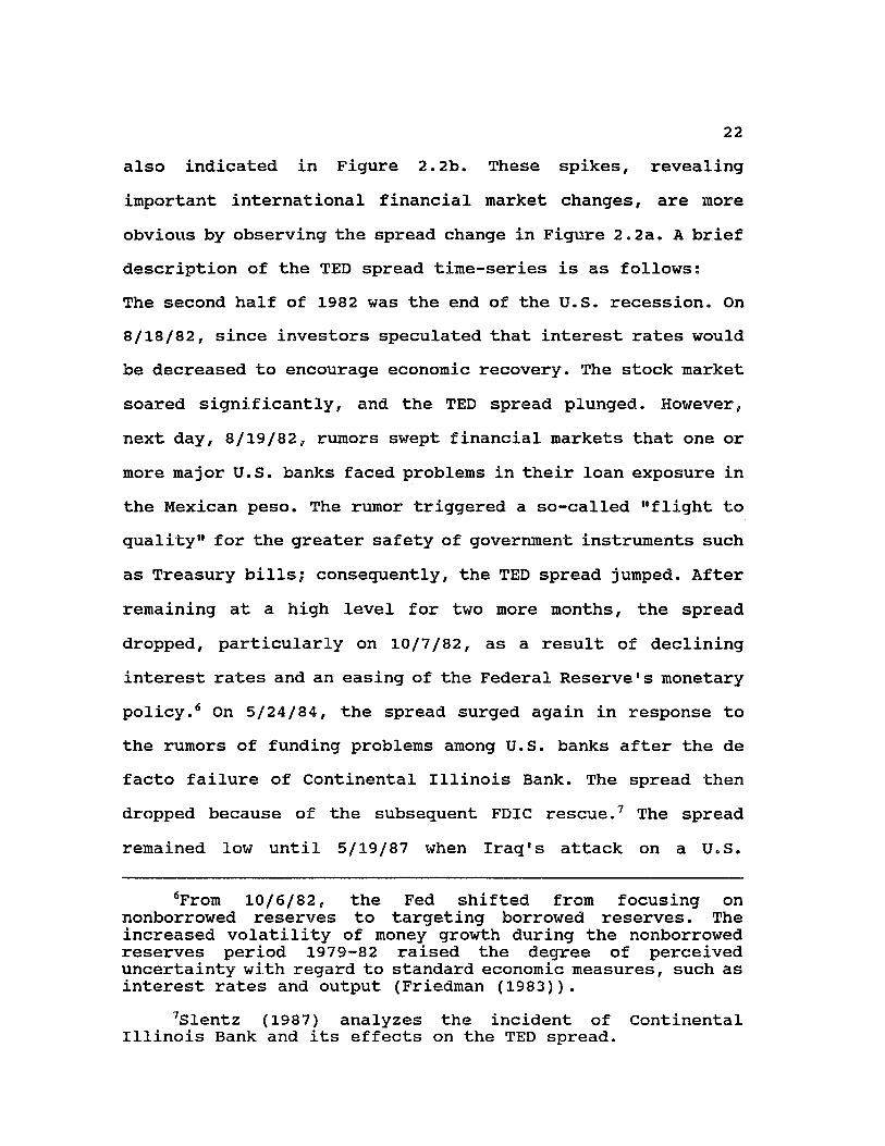
22

also indicated in Figure 2.2b. These spikes, revealing important international financial market changes, are more obvious by observing the spread change in Figure 2.2a. A brief description of the TED spread time-series is as follows:The second half of 1982 was the end of the U.S. recession. On 8/18/82, since investors speculated that interest rates would be decreased to encourage economic recovery. The stock market soared significantly, and the TED spread plunged. However, next day, 8/19/82, rumors swept financial markets that one or more major U.S. banks faced problems in their loan exposure in the Mexican peso. The rumor triggered a so-called "flight to quality" for the greater safety of government instruments such as Treasury bills; consequently, the TED spread jumped. After remaining at a high level for two more months, the spread dropped, particularly on 10/7/82, as a result of declining interest rates and an easing of the Federal Reserve's monetary policy.6 On 5/24/84, the spread surged again in response to the rumors of funding problems among U.S. banks after the de facto failure of Continental Illinois Bank. The spread then dropped because of the subsequent FDIC rescue.7 The spread remained low until 5/19/87 when Iraq's attack on a U.S.

6From 10/6/82, the Fed shifted from focusing on nonborrowed reserves to targeting borrowed reserves. The increased volatility of money growth during the nonborrowed reserves period 1979-82 raised the degree of perceived uncertainty with regard to standard economic measures, such as interest rates and output (Friedman (1983)).

7Slentz (1987) analyzes the incident of Continental Illinois Bank and its effects on the TED spread.

frigate, which was protecting Kuwaiti ships in the Persian Gulf, created uncertainty. This surge was followed by the well-known stock market crash (Black Monday) on 10/19/1987, when investors feared that epidemic defaults among securities and futures traders might endanger the bank solvency. Since no important international news happened for the period 1988- 1990, the TED spread was relatively stationary. Then in January 1991, the eruption of the Persian Gulf War jolted the world's financial markets; and, accordingly, the TED spread rose substantially. But on 1/17/91, speculation that U.S.-led forces in the Gulf War were headed for a quick victory triggered an explosive bond market rally. The ED yields and the spread that had been rising because of the war then dropped substantially. Afterward, the spread was fairly stationary except the spike on 11/16/92. On that day, the weak fundamentals were aggravated by Japan's political scandal; the Tokyo stock prices, as well as other major international stock prices, dropped broadly.

The previous paragraph provides evidence that the TED spread reflects the soundness of the international financial market. More importantly, the TED spread can play a major role in transmitting changes in the supply and demand for the Eurodollar tirae-deposit and Treasury bill markets (Siegel and Siegel (1989, p.265-266)). Thus there are theoretical reasons for the TED spread to play an integral role in the cointegration vector discussed in the following sections.

2 4

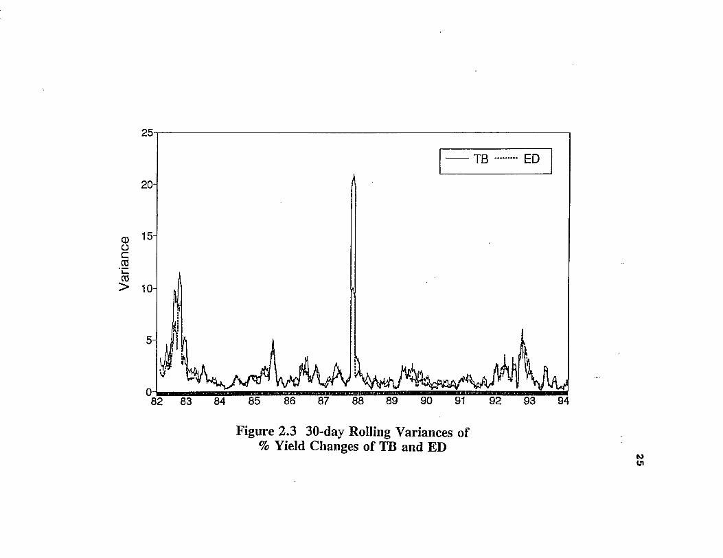
In recent years, it is often argued that the Eurodollar market is more sensitive than its U.S. counterpart to changes in domestic credit conditions because of the existence of fewer regulatory constraints in the international money markets; hence, U.S. rates adjust more slowly to changing conditions than do Eurodollar rates. Nonetheless, if the volatility is assumed to be driven by the arrival of information, this argument is not supported by the result reported in Panel B of Table 2.1. It shows that the variances of percentage yield changes (both close-to-close and open-to- close) of TB are statistically higher than ED, though these results are less significant for the post-crash period. Particularly, the open-to-close variances are statistically the same. An observation of Figure 2.3 illustrating the 30-day rolling variance of percentage yield changes also evinces that TB yields are more volatile than ED yields before and during the crash, while they are comparatively volatile to each other for the post-crash market. Taking together these preliminary results, it may be argued that the U.S. rates incorporate information at a faster speed than the Eurodollar rates in the period 1982-1987, but at the same speed after the crash.

2.4 Cointegration Analysis

Cointegration methodology is used to explore the relationship between the TB and ED yields. If TB and ED yields are nonstationary and need to be differenced to induce

Var

ianc

e25

EDTB

20-

15-

10-

89 9285 888483

Figure 2.3 30-day Rolling Variances of % Yield Changes of TB and ED

26stationarity, which implies the presence of a unit root, and there exists a linear combination of TB and ED yields that is stationary; the two yield series are said to be cointegrated. If cointegration is obtained, Granger-cause models must explicitly recognize the phenomenon or they will be misspecified. The theory of cointegration is fully developed in Granger (1986) and Engle and Granger (1987).

2.4.1 Testing for IntegrationAugmented Dickey-Fuller (ADF) (Dickey and Fuller, 1979;

1981) unit root test statistics are computed for the TB and ED yields. In the literature, the order of lagged differences, p, is usually chosen arbitrarily so that the residual of the regression model is white noise. However, Schwert (1987) points out that an inappropriate choice of lag order will too frequently lead to the conclusion of stationarity. In this chapter, the high-order autoregressive test proposed by Said and Dickey (1984) is used. The lag length formula for this test is presented in (1) and is shown by Schwert (1987) to be less affected by different data-generating processes:

p = Jnfc{1 2 (T/100)1/4}, (1)

where Int is the integer function. (1) is consistent with the theory that the optimal value of p increases slowly with the sample size, T. The lag is 27 and 23, respectively, for the whole period and each subperiod. To complement the ADF test,

2 7

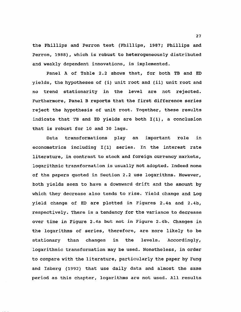
the Phillips and Perron test (Phillips, 1987; Phillips and Perron, 1988), which is robust to heterogeneously distributed and weakly dependent innovations, is implemented.

Panel A of Table 2.2 shows that, for both TB and ED yields, the hypotheses of (i) unit root and (ii) unit root and no trend stationarity in the level are not rejected. Furthermore, Panel B reports that the first difference series reject the hypothesis of unit root. Together, these results indicate that TB and ED yields are both 1(1), a conclusion that is robust for 10 and 30 lags.

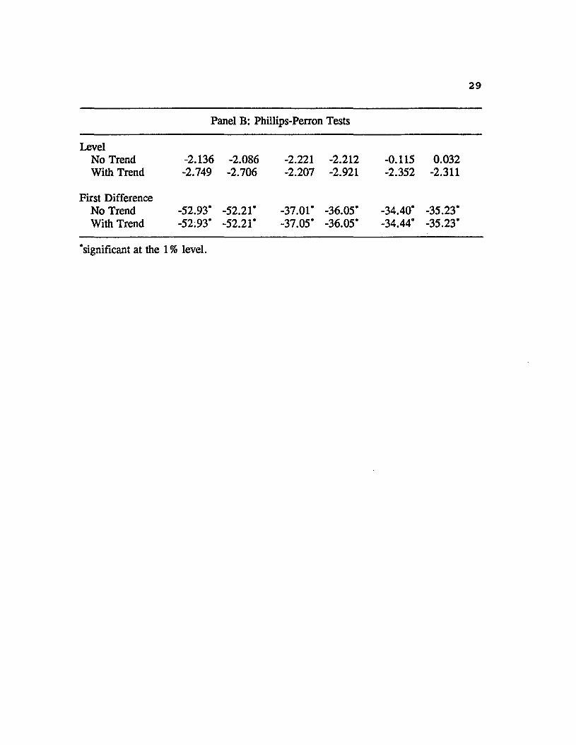
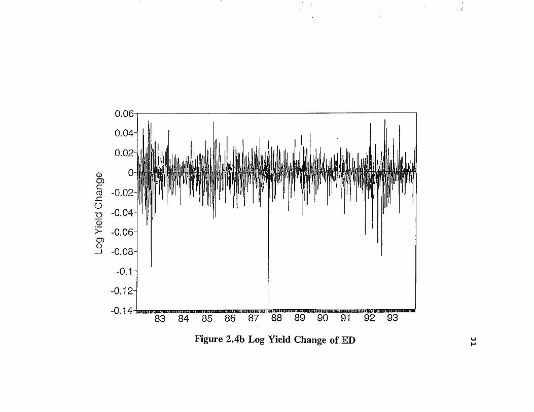
Data transformations play an important role in econometrics including 1(1) series. In the interest rate literature, in contrast to stock and foreign currency markets, logarithmic transformation is usually not adopted. Indeed none of the papers quoted in Section 2.2 use logarithms. However, both yields seem to have a downward drift and the amount by which they decrease also tends to rise. Yield change and Log yield change of ED are plotted in Figures 2.4a and 2.4b, respectively. There is a tendency for the variance to decrease over time in Figure 2.4a but not in Figure 2.4b. Changes in the logarithms of series, therefore, are more likely to be stationary than changes in the levels. Accordingly, logarithmic transformation may be used. Nonetheless, in order to compare with the literature, particularly the paper by Fung and Isberg (1992) that use daily data and almost the same period as this chapter, logarithms are not used. All results

28Table 2.2

Results of the ADF Unit Root Tests Entries are the statistics for the two hypotheses: (i) H^i): unit root; (ii) H^ii): unit root (with trend). The critical values for Hc(i) and H0(ii) of the ADF and Phillips-Perron tests using the 1% level are -3.43 and -3.96, respectively. These values are obtained from Fuller (1976, p.373) and Dickey and Fuller (1981, Table VI).For the ADF tests, the following OLS regressions are performed for hypotheses (i) and (ii) respectively:

piXt = a o+ a1Xt_1 + ) 0 iAXt_1 + e t ,

i-1P

= a o + aixt-i + a2 c + 0 i^t-x + e t'

p is 23 as obtained by Schwert (1987). The Phillips and Perron tests involve computing the following two OLS regressions:

X t = \im + v lx t_1 + VtX t = |i + v2(t-r/2) + v1*t_1 + S t

The hypothesis of unit root is H„(i): Pi=l ; the hypothesis of unit root and no trend stationarity is H„(ii): vt = l. The statistics require consistent estimates of the variances of the sums of the innovations £,* and £,. Perron (1988, Table 1) provides the detailed algebraic expressions of the statistics.

3/1/82 - 2/22/94 3/1/82 - 9/30/87 (Pre-Crash)

1/4/88 - 6/30/93 (Post-Crash)

TB ED TB ED TB ED

Panel A: ADF Tests

Level No Trend With Trend

-2.513-3.024

-2.476-2.969

-2.488-2.183

-2.519-2.282

-0.150-3.042

0.017-3.090

First Difference No Trend With Trend

-10.65’-10.69*

-11.27*-11.29*

-7.987*-8.123*

-7.682*-7.834*

-7.055*-7.277*

-7.056*-7.272’

with H0(i) : ax = 0;

with H0(ii) : a1 = 0;

(table con’d.)

29

Panel B: Phillips-Perron Tests

LevelNo Trend -2.136 -2.086 -2.221 -2.212 -0.115 0.032With Trend -2.749 -2.706 -2.207 -2.921 -2.352 -2.311

First DifferenceNo Trend -52.93* -52.21* -37.01* -36.05* -34.40* -35.23*With Trend -52.93* -52.21* -37.05* -36.05* -34.44* -35.23*

‘significant at the 1 % level.

Yield

C

hang

e

0.40 -

0.00-

0.40 -

0.60 -

0.80 -

1.00-

■1.2083 84 85 86 87 88 89 90 91 92 93

Figure 2.4a Yield Change of ED uo

Log

Yield

C

hang

e0 .0 6

0.04

0.021

- 0.021

-0.041

- 0.061-O.O81

-0.1H

- 0.121

-0.14

Figure 2.4b Log Yield Change of ED

32using logarithms, however, are qualitatively the same with some minor differences that will be discussed later.

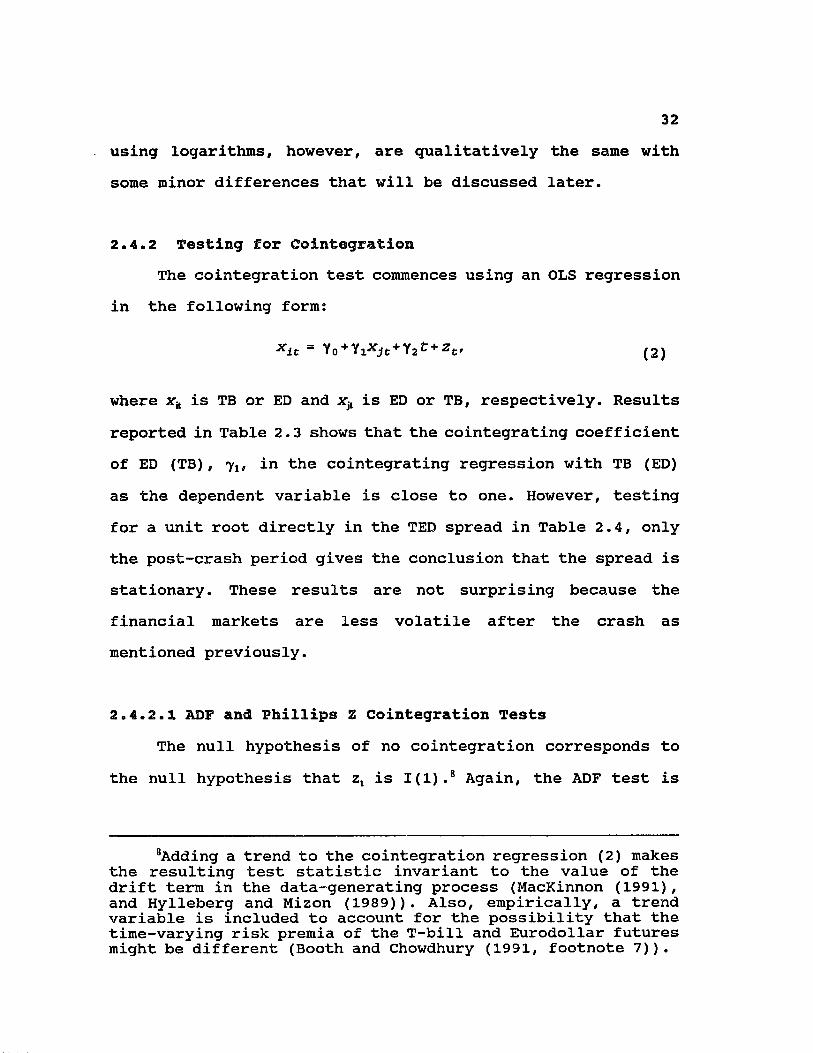
2.4.2 Testing for CointegrationThe cointegration test commences using an OLS regression

in the following form:

xit = Y0 + Yi*jt + Y2fc+zt, (2)

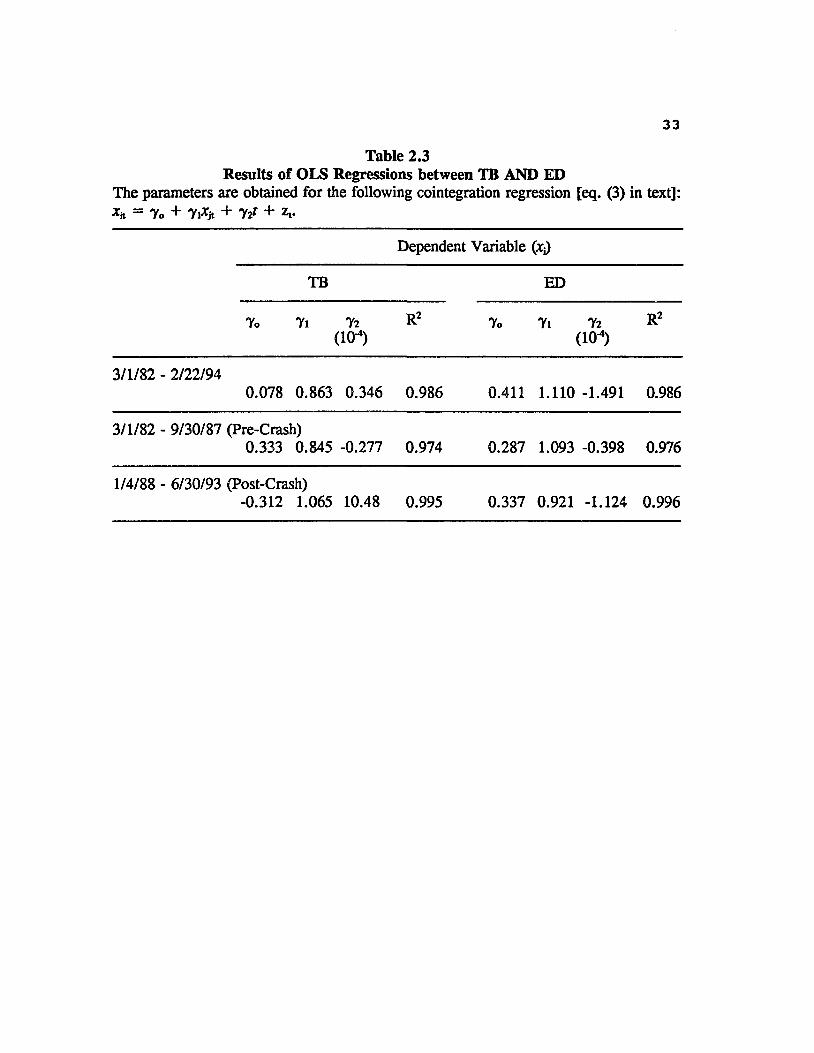
where xk is TB or ED and x^ is ED or TB, respectively. Results reported in Table 2.3 shows that the cointegrating coefficient of ED (TB), 7j, in the cointegrating regression with TB (ED) as the dependent variable is close to one. However, testing for a unit root directly in the TED spread in Table 2.4, only the post-crash period gives the conclusion that the spread is stationary. These results are not surprising because the financial markets are less volatile after the crash as mentioned previously.

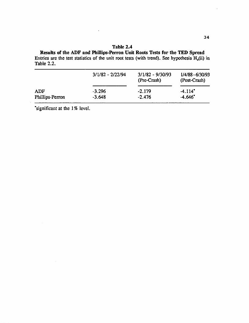
2.4.2.1 ADF and Phillips Z Cointegration TestsThe null hypothesis of no cointegration corresponds to

the null hypothesis that zt is 1(1).8 Again, the ADF test is

8Adding a trend to the cointegration regression (2) makes the resulting test statistic invariant to the value of the drift term in the data-generating process (MacKinnon (1991), and Hylleberg and Mizon (1989)). Also, empirically, a trend variable is included to account for the possibility that the time-varying risk premia of the T-bill and Eurodollar futures might be different (Booth and Chowdhury (1991, footnote 7)).

33Table 2.3

Results of OLS Regressions between TB AND ED The parameters are obtained for the following cointegration regression [eq. (3) in text]: X* = 7o + 7i*jt + 7it + z».

Dependent Variable (Xj)TB ED

7o 7i 72 R2 7o 7i 72 R2(io4) (10)

3/1/82 - 2/22/940.078 0.863 0.346 0.986 0.411 1.110 -1.491 0.986

3/1/82 - 9/30/87 (Pre-Crash)0.333 0.845 -0.277 0.974 0.287 1.093 -0.398 0.976

1/4/88 - 6/30/93 (Post-Crash)-0.312 1.065 10.48 0.995 0.337 0.921 -1.124 0.996

34Table 2.4

Results of the ADF and Phillips-Perron Unit Roots Tests for the TED SpreadEntries are the test statistics of the unit root tests (with trend). See hypothesis H^ii) in Table 2.2.

3/1/82 - 2/22/94 3/1/82 - 9/30/93 1/4/88 - 6/30/93(Pre-Crash) (Post-Crash)

ADF -3.296 -2.179 -4.114*Phillips-Perron -3.648 -2.476 -4.646*


35used. Moreover, the asymptotic critical value is also available in Phillips and Ouliaris (1990) based on the Phillips' (1987) Za and Zt tests. In this chapter, the Za test (or simply Z test) is employed because of its superior power properties. Cointegration results are presented in Table 2.5. For the whole and pre-crash periods, both ADF and Phillips Z tests do not reject the null hypothesis of no cointegration-—

TB and ED yields are not cointegrated. For the post-crash period, in contrast, the Phillips Z test gives significant result of cointegration, while the ADF test provides cointegration evidence at the 5% level.

2.4.2.2 Johansen Cointegration TestsThe Granger Representation Theorem implies that any

cointegrated system may be written as a vector error correction model (VECM),

where Xt is Nxl vector of N 1(1) variables and II is NxN matrix that has reduced rank if the variables in Xt are cointegrated. The next section discusses the error correction model in greater details. Johansen (1988, 1991) has developed themaximum likelihood estimators, trace and Am*, for a cointegrated system based on the technique of reduced rank regression to examine the null hypothesis of r cointegration

(3)

36Table 2.5

Results of the ADF and Phillips Z Cointegration Tests The ADF test requires estimation of the following model:

23Azt = $zt_x + g (p jAZe_1 + et,

with H0: <J> = 0. Zj is derived from eq.3 in text. The critical value is reported inMacKinnon (1991, Table 1); the 1% level is -4.33. The critical value of Phillips Z test is obtained in Phillips and Ouliaris (1990, Table lc); the 1% level is -35.42%. See Phillips and Ouliaris (1990) for detailed description of Z test in cointegration.

3/1/82 - 2/22/94 3/1/82 - 9/30/93 (Pre-Crash)

1/4/88 - 6/30/93 (Post-Crash)

Dependent Variable*

TB ED TB ED TB ED

ADF -3.513 -3.505 -1.968 -1.280 -4.141 -4.167

ADF-White -2.289 -2.245 -1.326 -1.386 -3.081 -3.146

Phillips Z -35.20 -35.02 -14.49 -14.02 -43.09* -43.00*

•Dependent Variable in eq. (2) in text, ‘significant at the 1 % level.

37vectors. [See Johansen (1988, 1991) for detailed discussion of the estimation technique.] Gonzalo's (1994) Monte Carlo results show that these estimators are robust to differing error structures and produce superior inference with respect to other estimates, particularly the ADF tests.

Reimers (1991) finds that the SIC performs well in selecting the lag length k in the VECM. Nonetheless, sufficient lags of Axt have to be imposed to whiten the residuals in each differenced equation. For each period, the SIC chooses k=2. However, since the residuals of the ATB equations are autocorrelated for k=2. Higher lags (also chosen by the SIC) with no autocorrelation are used: for the whole period, Jc=8, and k=3 for each subperiod.

Table 2.6 illustrates that TB and ED are cointegrated for the whole period as the trace and test statistics for the null hypothesis of r=0 are both significant. However, neither subperiod gives significant results as shown by both statistics. Hence, the Johansen test provides consistent results with the ADF and Phillips Z tests for the pre-crash period, but not for the whole and post-crash period. If results obtained from the Johansen test are believed to be more reliable as the usual practice in the literature, it can be argued that TB and ED are cointegrated, and that Johansen test gives insignificant results for either subperiod can be explained by the fact that since cointegration is a long-run

38Table 2.6

Results of Johansen Cointegration Tests r represents the hypothesized number of cointegration vectors in Xv Critical values are obtained from Osterwald-Lanum (1992, Table 1.1*). The 1% levels are 23.52 and 19.19 for the trace and X^, respectively.

if H0: r=0 H0: r= l P-Value of Q(12)-stat.b

trace X ^ trace X ^ ATB AED

3/1/82 - 2/22/948 25.51* 20.15* 5.36 5.36 0.09 0.75

3/1/82 - 9/30/87 (Pre-Crash)3 18.60 13.99 4.71 4.71 0.06 0.51

1/4/88 - 6/30/93 (Post-Crash)3 14.32 13.92 0.40 0.40 0.21 0.09

*k chosen by the SIC is the lag length in the VECM. SIC = /n|Er Ar| + mln(T)/T, where t rN denotes the ML estimate of the residual covariance matrix and m — rf(k- i)+N+2Nr-r2 is the number of freely estimated parameters of the VECM. Similar results are obtained if the AIC is used.bLjung-Box Q-siatistic for 12th-order serial correlation in the residuals estimated from the first differenced regression adjusted for lagged ATB and AED. The insignificant Q- statistics distributed as indicate that the residuals are not autocorrelated, acondition that is required for Johansen tests.’significant at the 1 % level.

39relationship, subdividing the period definitely reduces the span of time and, accordingly, the power of the test.9

2.4.3 Conditional Heteroskedasticity and Cointegration TestsDespite the extensive literature on autoregressive

conditional heteroskedasticity (ARCH) of Engle (1982) and related models, relatively little attention has been given to the issue of the GARCH effects on the performance of cointegration tests. As aforementioned, both TB and ED have strong ARCH effects. The performance of cointegration tests in the presence of GARCH effects is worth examining. An extensive Monte Carlo experiment is conducted in the Appendix of the dissertation. In order to isolate the GARCH effects from nuisance parameters, only purely random walks (with no drift) are examined. Also, although the Phillips Z test is not examined in the experiment, its results should be similar to that of the DF test as both are based on regression residuals. It shows that the cointegration tests including the (A)DF and Johansen tests tend to over-reject the null hypothesis of no cointegration in favor of finding cointegration too often in the presence of GARCH errors, but the bias is not very serious except when the variance processes are nearly degenerate and integrated. Among all of the cointegration tests examined, the Johansen trace statistic has the best size and power

9Hakkio and Rush (1991) further argue that the performance of cointegration tests only depends on the span of time instead of number of observations.

40performance. Moreover, the DF test with the White (1980) heteroskedasticity correction (ADF-White) may improve the size of the test but has a very poor power performance.

Chapter 3 shows that both series follow a nearly degenerate and integrated GARCH process and the Appendix indicates that the degree of size distortion for this process is increased, not decreased, when the sample size is increased. Thus, the cointegration results given by the Johansen tests for the whole period is called into question. Applying the ADF tests with the White correction, Table 2.5 indicates that insignificant result is obtained for the postcrash period, as well as the whole and post-crash period, at the 5% level. Of course, these results may simply induced by the lower power of the ADF-White test. Inevitably, inconsistent results given by different cointegration tests warrant further investigation.10

10It is worth noting that all previous papers using the ADF test do not incorporate the White correction. In particular, the ADF test without White correction is the only cointegration test used in Fung and Isberg (1992). Moreover, they do not use White correction in the error correction models (discussed in next section), and the t-statistics of the error correction terms are only -3.0 and -2.3. Note that their sample size is 2003. Thus, their cointegration results are not very conclusive after taking into accounts of the GARCH effects and the Lindley Paradox.

412.5 Error Correction Model and Granger Causality

2.5.1 Theoretical BackgroundAs previously mentioned, any cointegrated system may be

written as an ECM. Note that the reverse is also true. Specifically, if at least one of the error correction term is significant, the series are cointegrated. Kremers, Ericsson, and Dolado (1992), among others, contend that this "reverse" approach of estimating the significance of error correction terms for testing cointegration is more appropriate. In fact, if the error correction term is insignificant, none of the theories for cointegration explained below can be maintained.

Assuming that TB and ED yields are cointegrated, according to the Granger Representation Theorem in Engle and Granger (1987), the residuals of the cointegration regression need to be included in the vector autoregression (VAR) of first differences as follows:

A TBt = ax + t>xzt_x + lagged(A TBt, LEDt) 4aj

A EDt = a2+b2zt_x + lagged(LTBt, AEDt) + e , , (4b)

where z, is the error correction term, e^t and e^, are joint white noise and with IbJ + l^l O.

The error correction model (ECM) (3) shows that although TB yields and ED yields diverge in the short run, they will move together in the long run. As suggested by Engle and Granger (1987), cointegration reflects the behavior of

economic forces interacting to obtain an equilibrium. Booth and Chowdhury (1991) extend this explanation by discussing the long-run dynamics in terms of equilibrium overshooting (in the Dornbusch et al. sense) between two similar assets. Nonetheless, the ECM does not necessarily imply that yields adjust because the spread between them is out of equilibrium. For instance, Campbell and Shiller (1987, 1988) illustrate, in the context of present value models, that cointegration occurs as a result of one time series anticipating another.11 Following the idea that in the term structure, the spreads might measure anticipated changes in yield; cointegration may imply that the TED spread provides agents with information for forecasting changes in TB and ED yields. Regardless of the reasons giving rise to cointegration, Granger and Escribano (1986), however, state that there must be Granger causality in at least one direction through the knowledge of ztA.

To allow for asymmetric error correction of the "disequilibrium" between series, the following asymmetric ECM is also estimated.

A TBt = ax + wx2z*t_x + wx2z~t_x + lagged{ATBt, AEDt) +era>, (5a)

A EDt = a2 + wzlz U + w22Zt-i + lagged(ATBc, AEDt) + eBD(t,

where z^+ = max{zt.,,0>, and zt.{ = max{-zt_lrO} (Granger and Lee

"Another interpretation is given by Granger (1988). He shows that cointegration measures the relationship among control, target, and dependent variables. See also Booth and Chowdhury (1992).

43(1988)). Since results given by the symmetric and asymmetric ECM are qualitatively the same, only the former is reported.

2.5.2 Estimation of Error Correction ModelIn estimating the model, it is necessary to include two

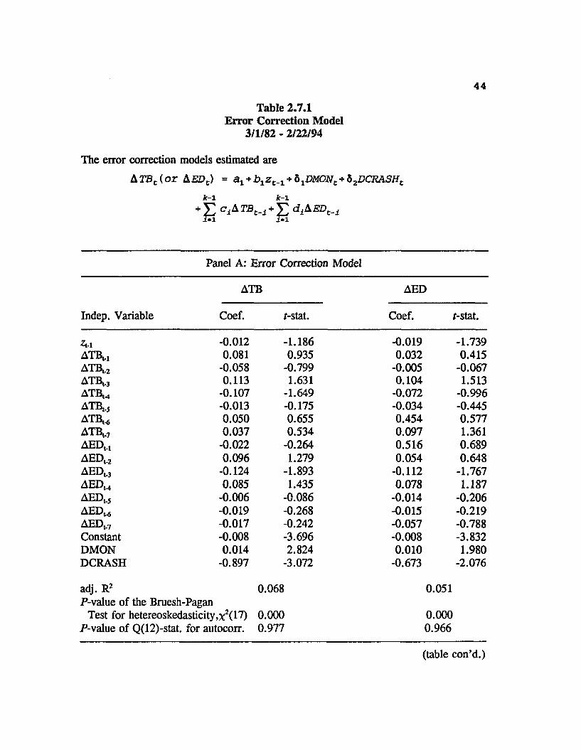
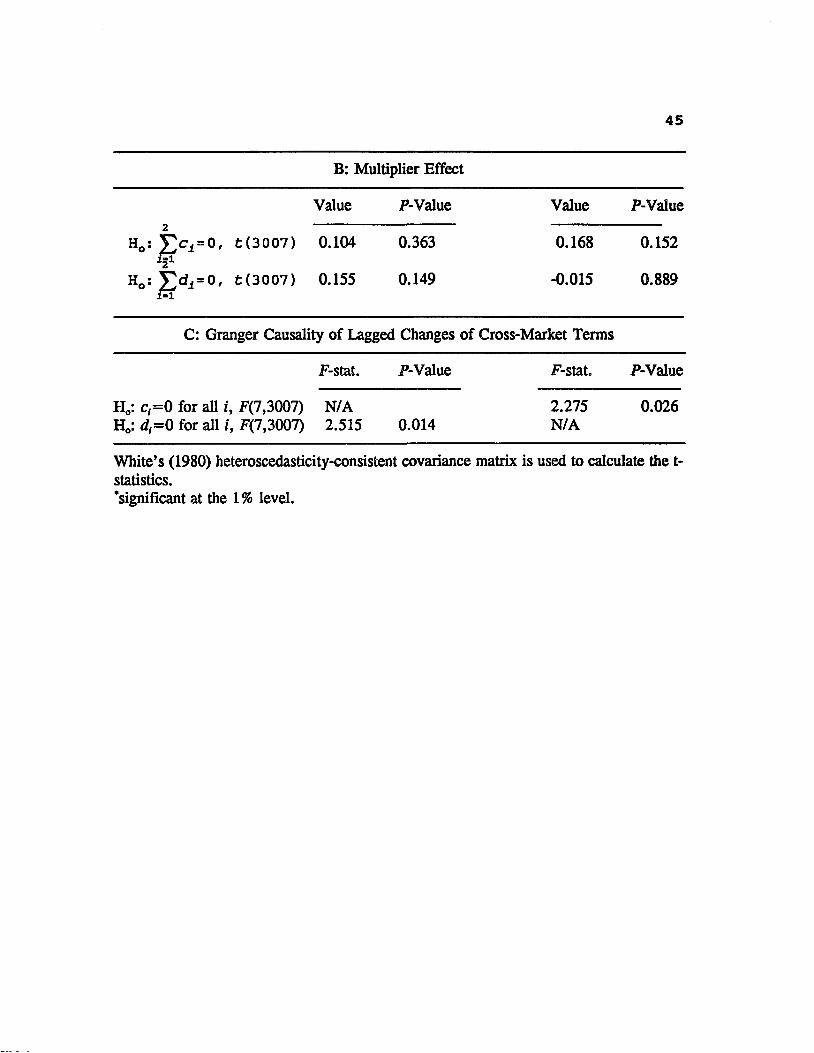
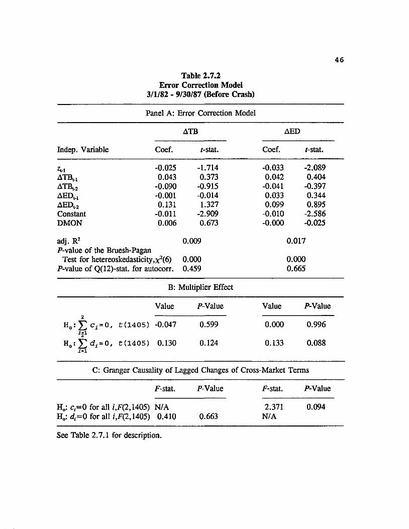
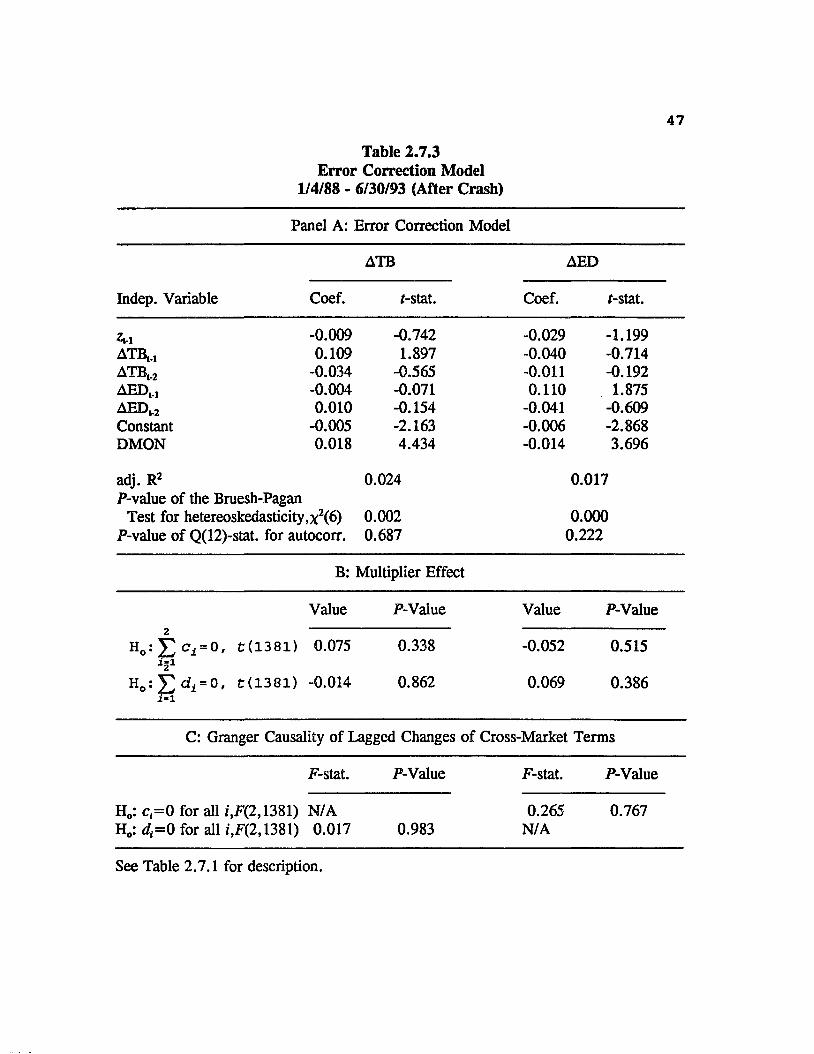
dummy variables to account for the October crash and the weekend effect. DCRASH represents a dummy variable that takes a value of 1 on October, 19 and 20, 1987 and 0 otherwise; DMON takes a value of 1 on days following weekends and holidays and 0 otherwise. Moreover, the residual derived from the cointegrating regression (4) with ED as the dependent variable is used. Because of this formulation, theoretically, the sign of error correction term in the TB model (i.e., TB yield change is used as the dependent variable in the ECM) should be positive, and that in the ED model negative. Tables 2.7.1-2.7.3 present the ECM with the lag length estimated by the SIC in Section 2. To account for the presence of heteroskedasticity in the ECM residuals, as indicated by the Bruesh-Pagan LM test, the reported t-statistics are derived from White's (1980) heteroskedasticity-consistent covariance matrix. The error correction term, zt.lf in each table is statistically insignificant in both the TB and ED models. These results suggest that TB and ED are not cointegrated for the whole period and each subperiod. The former result is contradictory to that of the Johansen test. Furthermore, the sign of the error correction term in the TB model in each

44Table 2.7.1

Error Correction Model3/1/82 - 2/22/94

The error correction models estimated areA TBt(or &EDt) = a2 + + b1DMONt + hzDCRASHt

Jt-l 1c-l+ V CjATB^ + V di ^EDt_i

i*l 1^1

Panel A: Error Correction Model

ATB AED

Indep. Variable Coef. r-stat. Coef. r-stat.

Zt-1 -0.012 -1.186 -0.019 -1.739atb,, 0.081 0.935 0.032 0.415atb,2 -0.058 -0.799 -0.005 -0.067atb, 3 0.113 1.631 0.104 1.513atb^ -0.107 -1.649 -0.072 -0.996atb.,5 -0.013 -0.175 -0.034 -0.445atb* 0.050 0.655 0.454 0.577ATBt.7 0.037 0.534 0.097 1.361AED„ -0.022 -0.264 0.516 0.689AEDt.2 0.096 1.279 0.054 0.648AED,3 -0.124 -1.893 -0.112 -1.767a ed m 0.085 1.435 0.078 1.187AED,5 -0.006 -0.086 -0.014 -0.206AED j -0.019 -0.268 -0.015 -0.219a ed ,.7 -0.017 -0.242 -0.057 -0.788Constant -0.008 -3.696 -0.008 -3.832DMON 0.014 2.824 0.010 1.980DCRASH -0.897 -3.072 -0.673 -2.076

adj. R2 0.068 0.051P-value of the Bruesh-Pagan

Test for hetereoskedasticity,x2(17) 0.000 0.000P-value of Q(12)-stat. for autocorr. 0.977 0.966

(table con’d.)

45

B: Multiplier Effect

Value P-Value Value P-Value2

t (3007) 0.104 0.363 0.168 0.152

H0: £ d i = 0, t (3007)l-i

0.155 0.149 -0.015 0.889

C: Granger Causality of Lagged Changes of Cross-Market Terms

F-stat. P-Value F-stat. P-Value

H0: c(= 0 for all i, F(7,3007) H0: <f(=0 for all i, F(7,3007)

N/A2.515 0.014

2.275N/A

0.026

White’s (1980) heteroscedasticity-consistent covariance matrix is used to calculate the t- statistics.'significant at the 1 % level.

46Table 2.7.2

Error Correction Model3/1/82 - 9/30/87 (Before Crash)


ATB AED

Indep. Variable Coef. f-stat. Coef. f-stat.

Zn -0.025 -1.714 -0.033 -2.089ATB,.! 0.043 0.373 0.042 0.404ATBj.2 -0.090 -0.915 -0.041 -0.397AED,.! -0.001 -0.014 0.033 0.344AED,.2 0.131 1.327 0.099 0.895Constant -0.011 -2.909 -0.010 -2.586DMON 0.006 0.673 -0.000 -0.025




Value P-Value Value P-Value2 ....

H0: 5 3 ^ = 0, t(1405) -0.047i*l

0.599 0.000 0.9962

K o ^ d ^ O , t (1405) 0.130 0.124 0.133 0.088



H0: cf= 0 for all i,F(2,1405) N/A 2.371 0.094H0: d(= 0 for all /,F(2,1405) 0.410 0.663 N/A

See Table 2.7.1 for description.

47Table 2.7.3

Error Correction Model1/4/88 - 6/30/93 (After Crash)


ATB AED


Zt.i -0.009 -0.742 -0.029 -1.199ATB,.! 0.109 1.897 -0.040 -0.714ATBt_2 -0.034 -0.565 -0.011 -0.192AED,.! -0.004 -0.071 0.110 1.875AED,,2 0.010 -0.154 -0.041 -0.609Constant -0.005 -2.163 -0.006 -2.868DMON 0.018 4.434 -0.014 3.696





£(1381) 0.0752*1

0.338 -0.052 0.5152

H o: S di = 0' t (1381) -0.014i-l0.862 0.069 0.386



H0: c,=0 for aU i\F(2,1381) N/A 0.265 0.767H0: 4 = 0 for aU /,F(2,1381) 0.017 0.983 N/A

See Table 2.7.1 for description.

48period is negative, which is inconsistent with the theory of ECM.

Two kinds of tests for the casual relationship are employed. First, multiplier effects of local and cross markets are tested. The multiplier is the sum of lag coefficients of TB or ED. It measures the total change in the dependent variable mean as a result of a unit change in the independent variable. Second, the Granger causality test is used to determine whether the lagged independent variable terms (i.e., lagged changes in the cross market) in the ECM have any significant impact on the dependent variable (i.e., current change in the local market). A Wald test is applied to test for statistical significance. The F-statistic of the first causality test which tests the null hypothesis that the sum of lagged coefficients is zero is less restrictive, while that of the second one tests zero restrictions on all lagged variables. The multiplier causality test seems to be more relevant in examining the causal relationship. For example, if the (strict) Granger causality test is significant but the multiplier causality test is not, it is still not very appropriate to conclude that lags of one series can predict the current value of other series.

Tables 2.7.1-2.7.3 shows that both of the cross-market terms, AED,., in the TB model and ATB,., in the ED model, are insignificant for each period. Multiplier and Granger causality tests also give insignificant result. Besides, the

49adjusted R2 in each case is less than 0.1. Hence, the ECM suggests that TB and ED are not cointegrated and do not Granger-cause each other, regardless of which period is analyzed.

Since the "true" lag structure of the ECM is unknown, trials for other specifications are necessary. Table 2.8.1-2.8.3 demonstrate the following results of the ECM with 23 lags: A. the error correction terms; C. Granger causality tests; and B. multiplier effects. Similar results are given by these general models, i.e., no cointegration and causality in either direction is found, wrong sign of the error correction term in the TB model, and small adjusted R2. An exception is the Granger-causality test for the post-crash period which indicate a bi-directional causality. However, since the multiplier tests are insignificant, the hypothesis of no lead/lag relationship, i.e., contemporaneous relationship, is not rejected.

To gain further insights into the causal relationship between TB and ED yields, the multiplier and Granger causality tests are applied in the 44 individual contracts for the whole period. For comparison with the results of Kaen, Halms, and Booth (1983) , equal lag lengths of two for both the dependent and independent variables are selected. However, only the last three months before maturity, excluding the delivery month, are used because of the two liquidity problems mentioned in Section 2.3. In addition, if the two individual futures

50Table 2.8.1

Error Correction Model with Lag Lengths of 233/1/82 - 2/22/94


ATB AED


Zn -0.008 -0.893 -0.014 -1.485

adj. R2 0.089 0.079


Value P-Value Value P-Value2 --

He: £ = 0 , t (2959) 0.501 0.026 0.528 0.0242

Ho: £ di = 0' t (2959) -0.283 1 1

0.164 -0.202 0.338



Ho:c,=0 for all i,F(23,2959) N/A Ho:d,=0 for all i,F(23,2959) 2.776 0.000

2.773N/A

0.000

Table 2.8.2Error Correction Model with Lag Lengths of 23

3/1/82 - 9/30/87 (Before Crash)

51


ATB AED


Zt-l -0.021 -1.668 -0.026 -1.895

adj. R2 0.024 0.036



Hc: £ C i = 0, t(1342) i21

Ho: £ di = 0' t(1342)i-1

0.349

-0.206

0.350

0.524

0.422

-0.164

0.280

0.631



Ho:c,=0 for aU /,F(23,1342) N/A Ho:d,=0 for all i,F(23,1342) 0.410 0.663

1.911N/A

0.008

Table 2.8.3Error Correction Model with Lag Lengths of 23

1/4/88 - 6/30/93 (After Crash)

52


ATB AED


Z.-1 -0.010 -0.743 -0.024 -1.632

adj. R2 0.046 0.048



Ho: £ ci = 0' t (1318) i21

Ho: Z di = 0' t (1318)i-l

0.140

-0.007

0.639

0.980

-0.034

0.265

0.908

0.344


F-stat. F-Value F-stat. P-Value

Ho:c,=0 for all j\F(23,1318) N/A Ho:di=0 for all i,F(23,1318) 0.596 0.934

0.604N/A

0.929

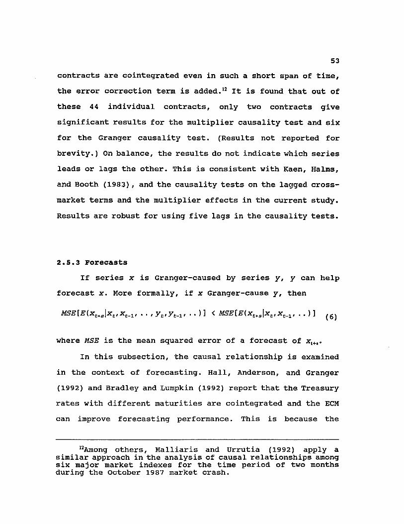
53contracts are cointegrated even in such a short span of time, the error correction term is added.12 It is found that out of these 44 individual contracts, only two contracts give significant results for the multiplier causality test and six for the Granger causality test. (Results not reported for brevity.) On balance, the results do not indicate which series leads or lags the other. This is consistent with Kaen, Halms, and Booth (1983) , and the causality tests on the lagged crossmarket terms and the multiplier effects in the current study. Results are robust for using five lags in the causality tests.

2.5.3 ForecastsIf series x is Granger-caused by series y, y can help

forecast x. More formally, if x Granger-cause y, then

MSE[E{.xt+g\xt., • • )] MSE[E(xt+g\xt, , • • )] gj

where MSE is the mean squared error of a forecast of x%+,.In this subsection, the causal relationship is examined

in the context of forecasting. Hall, Anderson, and Granger(1992) and Bradley and Lumpkin (1992) report that the Treasury rates with different maturities are cointegrated and the ECM can improve forecasting performance. This is because the

12Among others, Malliaris and Urrutia (1992) apply a similar approach in the analysis of causal relationships among six major market indexes for the time period of two months during the October 1987 market crash.

54existence of an ECM implies some Granger causality between the series, which suggests that the error correction model may be a useful forecasting tool.

The (unrestricted) VAR and ECM estimated by SIC for the whole and post-crash periods and those with lags 23 are used to obtain 155 one-step ahead forecasts over the period 7/1/93- 2/22/94. The forecasting performance of the VAR and ECM is compared to that of a naive no-change model by means of root mean squared error (RMSE) . The dummy variables discussed above are also included in the VAR and naive models. Table 2.9 indicates that both of the VAR and ECM give almost the same RMSE as the naive model. The difference is less than 1% among them. Hence, the VAR and ECM do not empirically give much improvement in forecasts even when compared with the naive model.

2.6 Contemporaneous Relationships and Simultaneous Equations Models

So far in this chapter, results do not support causality in either direction. While the hypothesis of contemporaneous relationship is not rejected, it is not vigorously sustained simply by using the VAR model (or ECM). This is because the VAR model is a reduced form model which omits the contemporaneous interaction. Thus if TB and ED are contemporaneously/structura1ly related on a daily basis, then the VAR model is misspecif ied and it yields biased and

55Table 2.9

Summary Statistics of One-Step Ahead Forecast Errors for the Period 7/1/93 - 2/22/94

This table compares the forecast performance measured by the root mean square errors (RMSE) of the VAR and error correction models estimated in Tables for the periods3/1/82 - 2/22/94 and 1/4/88 - 9/30/93. The forecasting period is 7/1/93 - 2/22/94.

DependentVariable

Model Mean(io-2) RMSE RMSE Ratio (104) (w.r.t naive model)

Panel A: 3/1/82 - 2/2/94

ATBj Naive 0.430 0.276 1.000VAR(7) 0.387 0.280 1.014VAR(23)) 0.375 0.284 1.029ECM(7) 0.352 0.281 1.018ECM(23) 0.357 0.285 1.032

aED, Naive 0.605 0.269 1.000VAR(7) 0.540 0.268 0.996VAR(23)) 0.530 0.271 1.007ECM(7) 0.485 0.267 0.993ECM(23) 0.497 0.271 1.007

Panel B: 1/4/88 - 2/22/94

ATBt Naive -0.035 0.277 1.000VAR(2) 0.022 0.272 0.982VAR(23) -0.008 0.280 1.011ECM(2) 0.083 0.272 0.982ECM(23) 0.096 0.279 1.007

aED, Naive 0.244 0.266 1.000VAR(2) 0.270 0.263 0.989VAR(23) 0.279 0.267 1.004ECM(2) 0.275 0.263 0.989ECM(23) 0.321 0.268 1.008

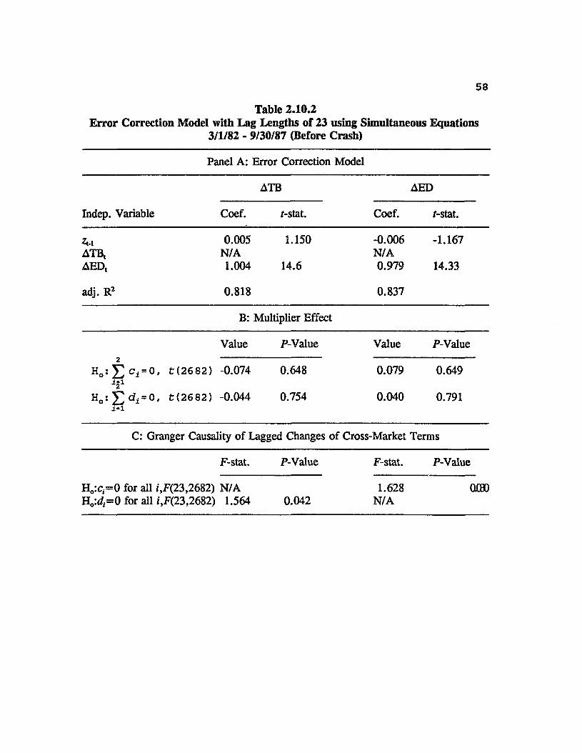
56inconsistent estimates of the structural dynamic linkages. This issue has been emphasized by Koch (1993) in stock index futures markets. As pointed out by Koch, when contemporaneous as well as lagged influences are included in a VAR-type model, the structural model becomes a dynamic simultaneous equation model (SEM) which requires an instrumental variables estimator to obtain consistent estimates.13 Moreover, the SEM can be interpreted as follows: "the contemporaneous coefficientsreflect the simultaneous interaction among variables, while the lagged coefficients reflect the lagged responses across variables after accounting for their contemporaneous interaction. (Koch(1993, p.1195))”

The SEM is estimated for each period and results are presented in Tables 2.10.1-2.10.3. Being consistent with contemporaneous relationships, the contemporaneous term, i.e., ATB, (AED,) in the AED, (ATB,) model, is highly significant and close to one, and the adjusted R2 is greater than 0.7. Note that the error correction term in the TB model gives a correct sign, positive, in all periods. More importantly, for the post-crash period, the t-statistics of zM in the TB and ED model are increased to 2.19 and -2.24, respectively, suggesting a feedback mechanism, though they are still not significant at the 1% level. In addition, according to the

13Using a SEM, Koch (1993) reexamines Chan and Chung's(1993) results of the intraday relationships associated with stock index futures markets. Some of his results are different from those of Chan and Chung.

57Table 2.10.1

Error Correction Model with Lag Lengths of 23 using Simultaneous Equations3/1/82 - 2/22/94


ATB AED

Indep. Variable Coef. /-stat. Coef. /-stat.

Zir l 0.003 0.754 -0.003 -0.857A T B , N/A N/AAED, 1.012 12.96 0.979 14.33

adj. R2 0.738 0.762

B : Multiplier Effect

Value P-Value Value P-Value

H o : E c i = 0 ' t ( 2 9 5 9 ) 0.054 0.684 -0.039 0.760¥

a

■M

H o t ( 2 9 5 9 ) -0.214 0.084 0.202 0.103



Ho:c,=0 for all i,F(23,2959) N/A 2.090 0.002Ho:4= 0 for all /,F(23,2959) 1.826 0.001 N/A

58Table 2.10.2

Error Correction Model with Lag Lengths of 23 using Simultaneous Equations3/1/82 - 9/30/87 (Before Crash)


ATB AED


Zm 0.005 ATB, N/A AED, 1.004

1.150

14.6

-0.006N/A0.979

-1.167

14.33

adj. R2 0.818 0.837


Value P-Value Value P-Value2 ' ......

Ho: 5 > i = 0 ' t*2682* -0.074 i 21

Ho: £ di = 0 ' fc<2682) -0.044i-l

0.648

0.754

0.079

0.040

0.649

0.791



Ho:c,=0 for all t,F(23,2682) N/A Ho:</,=0 for all i,F(23,2682) 1.564 0.042

1.628N/A

QJO0O

59Table 2.10.3

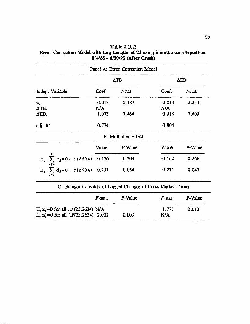
Error Correction Model with Lag Lengths of 23 using Simultaneous Equations8/4/88 - 6/30/93 (After Crash)


ATB AED


^ 0.015 ATB, N/A AED, 1.073

2.187

7.464

-0.014N/A0.918

-2.243

7.409

adj. R2 0.774 0.804


Value P-Value Value P-Value

Ho: V c i = 0, fc (2634) 0.176 0.209 -0.162 0.266

Ho: T d ^ 0 . t(2634) -0.291 0.054 0.271 0.047



Ho:c,=0 for all i,F(23,2634) N/A Ho:d,=0 for aU i,F(23,2634) 2.001 0.003

1.771N/A

0.013

60coefficient of zM , about 0.015, the half-life of the response of the TB or ED yield to a random shock is 46 days, a fairly slow adjustment process. Since the error terms are insignificant at the 5% level for the whole period and postcrash period, no such long-run dynamics exist.

In sum, results obtained from the SEM, which is less likely to be misspecified, suggest contemporaneous movement between TB and ED. A slow feedback mechanism may exist between them during the post-crash period, though the evidence is not very strong.

2.7 Fractional Cointegration

In the classical paradigm for cointegration, particularly the Johansen cointegration tests, all the members of the Xx vector are assumed to be 1(d) processes with d=l (or an integer) , while the cointegrating linear relationship a'Xt with a as the cointegrating vector is presumed to be I(d-Jb) with b=1. This is referred to as Cl(1,1) , which is also the case discussed in the chapter. The Granger Representation Theorem, nevertheless, only requires that the linear combination a'Xt be stationary, and, therefore, the discrete options 1(1) and 1(0) are rather restrictive. Particularly, in order to be mean-reverting, zt does not have to be 1(0) strictly; fractionally integrated processes introduced by Granger and Joyeus (1980) and Hosking (1981) also exhibit mean reversion. In this case the error correction term responds more slowly to

61shocks so that deviations from equilibrium are more persistent. The error correction term is depicted to possess long memory. In addition, it follows from Yajima (1988) and Cheung and Lai (1993b) that if all elements of Xt are 1(1) and they are fractionally cointegrated, the OLS estimator of a! is consistent and converges at the rate of T 1 .

Geweke and Porter-Hudak (1983) (GPH) propose a semi- nonparametric procedure to test for fractional integration. The procedure is motivated by the log spectral density of the fractionally integrated process, and amounts to estimating the OLS regression

ln{P (o) j) = P0 + P1ln{4sin2 (w^/2)} + T|

with /?!=-<?, where P( •) is the periodogram of the series at frequency «j. Geweke and Porter-Hudak (1983) recommend choosing the number of low-frequency periodogram ordinates, n, used in the spectral regression to be n=T' with v=0.50 or 0.55.

The Appendix of the dissertation provides a detailed analysis of fractional integration, fractional cointegration, and the GPH test. The potential bias induced by the GARCH effects on the fractional cointegration tests are also investigated in this Appendix. It is found that the size distortion is generally smaller than those of Johansen and ADF tests. For example, when a=0.1, and a+/3=0.999 in the conditional variance equation of the GARCH(1,1) model, (See Chapter 3 and the Appendix for more explanation), the size of

62the trace statistic at 5% is 11%, but only 9% for the GPH test. Moreover, Cheung and Lai (1993b) report that the GPH test has a better power performance than Johansen and ADF tests for fractionally integrated processes.

In short, the Johansen test, as well as the ADF test, does not allow for fractional cointegration between TB and ED such that the equilibrium error between them follows a fractionally integrated process instead of an exact 1(0) process. It is worth mentioning that including an intercept in the Johansen test, Diebold, Gardeazabal, and Yilmaz (1993) refute the significant cointegration result among seven nominal exchange rates in the paper by Baillie and Bollerslev(1989). However, Baillie and Bollerslev* s (1993) further analysis of error correction term suggests that it is well described as a fractionally integrated process with d=0.89, i.e., the rates are fractionally cointegrated. Thus, the fractional cointegration relationship analyzed in the next subsection may give a better understanding of the relationship between the two markets.

2.7.1 Empirical Results2.7.1.1 Unit Roots Using the GPH Test

Diebold and Rudebusch (1991) and Sowell (1990) show that the ADF test has low power against fractional integration alternatives. In this chapter, therefore, the GPH test is used to test for unit roots. The GPH test is used to estimate the

63differencing operator d in the first difference of the relevant series, (1 -L)hrA where wft = Axit and xit is TBt or ED,. As d of the level series equals 1+d, a value of d (d) not significantly different from zero (one) corresponds to a unit root in xit.

The values of d=l+d estimated by the periodogram OLS regression (7) on wit presented in Table 2.11 for the whole and the two subperiods are not significantly different from one, except for the TB yield in the subperiods with v=0.50 which gives a value of d=l.4. Hence, the hypothesis of a unit root (or higher order) is not rejected for either level series, a finding that is consistent with the previous unit roots results.

2.7.1.2 Fractional CointegrationThe equilibrium error, zt, is given by the cointegrating

regression (3). As pointed out by Cheung and Lai (1993b), in testing for fractional cointegration, the critical values for the GPH tests derived from the standard distribution cannot be used directly to evaluate the GPH estimate of d. The reason is that the equilibrium error, z„ is given by the OLS regression (3) which minimizes the residual variance; accordingly, the residual series estimated tends to bias toward being stationary. Therefore, the critical values for testing fractional cointegration between TB and ED are obtained from the Monte Carlo experiment in 10,000 replications with the

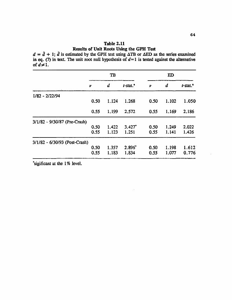
64Table 2.11

Results of Unit Roots Using the GPH Test d = d + 1; <5 is estimated by the GPH test using ATB or AED as the series examined in eq. (7) in text. The unit root null hypothesis of d = l is tested against the alternative of d& l.

TB ED

V d f-stat.® V d f-stat.®

1/82 - 2/22/940.50 1.124 1.268 0.50 1.102 1.050

0.55 1.199 2.572 0.55 1.169 2.186

3/1/82 - 9/30/87 (Pre-Crash)0.500.55

1.4221.123

3.427*1.251

0.500.55

1.2491.141

2.0221.426

3/1/82 - 6/30/93 (Post-Crash)0.500.55

1.3571.183

2.896*1.834

0.500.55

1.1981.077

1.6120.776

’sigificant at the 1 % level.

65same sample sizes, 3032 for the whole period and 1500 for the two sub-periods. The results are presented in Table 2.12, which shows that the critical value generated for testing the null hypothesis of no (fractional) cointegration of d=l against the one-sided alternative of del are greater in magnitude than the standard t-statistics.14 The critical values for the cointegrating regression with no trend are reported for reference only.

For the whole period, d of zt according to eg. (7) is estimated to be less than one (about 0.78), implying that zt is mean-reverting. As shown in Table 2.13 Panel A, this result is robust to the norma 1 i z at ion of eq. (2) and the choice of v. Nevertheless, the t-statistics for all cases are not significant at the 1% level (though some are significant at the 5%) ; hence, evidence showing long memory between TB and ED is not conclusive. Most importantly, the table indicates that the long memory evidence is much stronger during the postcrash period. In particular, d in the post-crash period is 0.68 on average and significantly less than one in each case, except one which is significant at the 5% level, while that in the pre-crash period is 0.95 and not significantly different from one. In short, TB and ED are found to be fractionally cointegrated, but this long-memory relationship is only obtained in the post-crash period. These results are analogous

14This may be simply inferred from the negative skewness of the distribution.

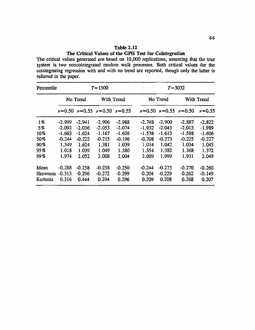
66Table 2.12

The Critical Values of the GFH Test for Cointegration The critical values generated are based on 10,000 replications, assuming that the true system is two noncointegrated random walk processes. Both critical values for the cointegrating regression with and with no trend are reported, though only the latter is referred in the paper.

Percentile T-= 1500 T= 3032

No Trend With Trend No Trend With Trend

*'=0.50 v=0.55 *=0.50 *=0.55 *=0.50 *=0.55 *=0.50 *=0.55

1% -2.999 -2.941 -2.906 -2.988 -2.748 -2.900 -2.887 -2.8225% -2.092 -2.036 -2.053 -2.074 -1.932 -2.043 -2.013 -1.98910% -1.663 -1.624 -1.167 -1.626 -1.538 -1.613 -1.588 -1.60650% -0.244 -0.222 -0.215 -0.196 -0.208 -0.273 -0.225 -0.22790% 1.349 1.624 1.381 1.039 1.014 1.042 1.034 1.04595% 1.018 1.039 1.049 1.380 1.354 1.382 1.368 1.37299% 1.974 2.052 2.008 2.004 2.009 1.999 1.931 2.049

Mean -0.288 -0.258 -0.258 -0.250 -0.244 -0.273 -0.270 -0.260Skewness -0.313 -0.296 -0.272 -0.299 -0.204 -0.229 -0.262 -0.149Kurtosis 0.316 0.444 0.294 0.296 0.209 0.208 0.268 0.207

67Table 2.13

Results of Fractional Cointegration Using the GPU Test d = 2 + 1; 3 is estimated by the GPH test using AZt as the series examined in eq. (7) in text. Results are virtually the same if d is directly estimated from the level z,.The no (fractional) cointegration null hypothesis of d = l is tested against the one-sided long-memory alternative of d <1. Critical values are based on the simulated values reported in Table 2.12. The only difference between Panel A and Panel B is that Panel B uses logarithmic transformation.

Dependent Variable

TB ED

V d r-stat. v d r-stat.

Panel A

3/1/82 - 2/22/940.500.55

0.7400.786

-2.662-2.758

0.500.55

0.7840.783

-1.951-2.530

3/1/82 - 9/30/87 (Pre-Crash)0.500.55

0.9990.902

-0.007-0.999

0.500.55

0.9620.919

-0.312-0.821

1/4/88 - 6/30/93 (Post-Crash)0.500.55

0.6750.699

-2.638-3.014*

0.500.55

0.6420.686

-2.907*-3.153*

Panel B: With Logarithmic Transformation

3/1/82 - 2/22/940.500.55

0.7520.767

-2.539-3.008*

0.500.55

0.7540.763

-2.520-3.057*

3/1/82 - 9/30/87 (Pre-Crash)0.500.55

0.9990.902

-0.007-0.999

0.500.55

0.9620.919

-0.312-0.821

1/4/88 - 6/30/93 (Post-Crash)0.500.55

0.5320.647

-3.919*-3.655*

0.500.55

0.6570.703

-2.867*-3.072*


68to the previous finding of a slow feedback mechanism using the simultaneous equations models.

For expository reasons, the first 120 autocorrelation coefficients p's of zt, as well as the series in level and in first difference for the post-crash period are elicited in Table 2.14. The extremely slow decline, if any, of the autocorrelation coefficients of both level series [with p (1)=0.99, p (60)=0.89, and p (120)=0.76], and the small coefficients of any lags of the first differenced series suggest that TB and ED follow a 1(1) process. If contrast, the autocorrelation coefficients of zt at lags up to 3 are still greater than 0.9, but the coefficients afterward are slowly declining to a value of 0.269 at lag 60 and -0.023 at lag 120.

In section 2.4, the data transformation problem is discussed. Log transformation does not qualitatively affect the results in the chapter. In there is any change, then the fractional cointegration evidence is even stronger for the post-crash period as shown in Table 2.13 Panel B*— the value of d for zt is lower and t-statistics are greater (in magnitude).

2.7.2 Derivations of Long MemoryAs previously mentioned, a cointegration system can be

represented by an ECM. This theorem is also valid for fractional cointegration, and theoretically, eq. (4) is simply modified to allow for fractionally integrated zt. However, empirically, incorporating a fractionally integrated error

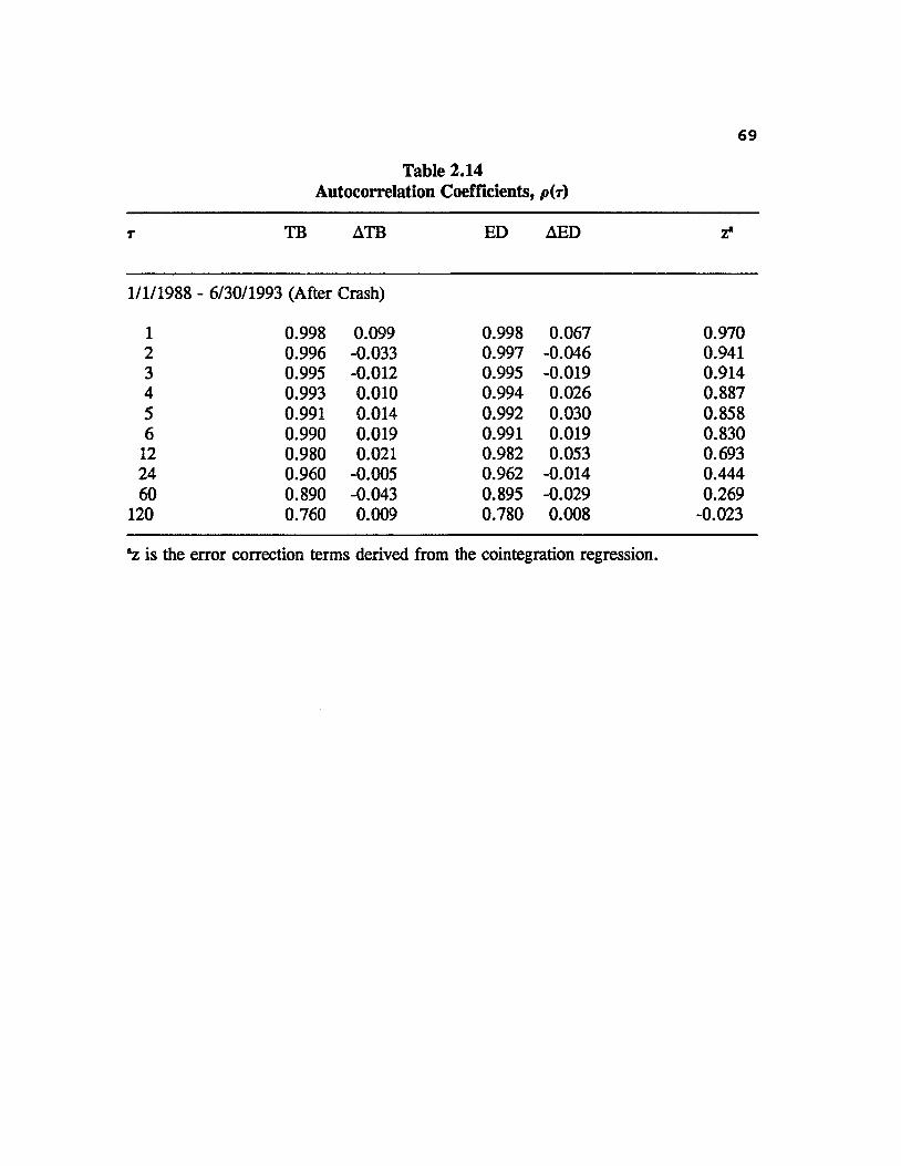
69Table 2.14

Autocorrelation Coefficients, p(r)

r TB ATB ED AED z*

1/1/1988 - 6/30/1993 (After Crash)

1 0.998 0.099 0.998 0.067 0.9702 0.996 -0.033 0.997 -0.046 0.9413 0.995 -0.012 0.995 -0.019 0.9144 0.993 0.010 0.994 0.026 0.8875 0.991 0.014 0.992 0.030 0.8586 0.990 0.019 0.991 0.019 0.830

12 0.980 0.021 0.982 0.053 0.69324 0.960 -0.005 0.962 -0.014 0.44460 0.890 -0.043 0.895 -0.029 0.269

120 0.760 0.009 0.780 0.008 -0.023

"z is the error correction terms derived from the cointegration regression.

70correction term in the ECM has not been developed in the literature.

Since TB and ED are found to be fractionally cointegrated in the post-crash period, there must be Granger causality in at least one direction. This contradicts the efficient market hypothesis, assuming informational efficiency. But Granger and Newbold (1986, p.226) argue that if the series are cointegrated, a further possible explanatory variable to account for changes in the long run is suggested. Risk premium may be one, and this is consistent with market efficiency. Nonetheless, daily data are used in the chapter and Lehmann(1990) argues that any systematic short-run changes in fundamental values should not occur in efficient markets. As a result, the sources of long memory explored are not explicitly determined.

2.8 Conclusions

Characteristics of the Treasury bill and Eurodollar futures markets (high liquidity, low transaction costs and institutional restrictions, same trading hours and exchange) offer a more reliable analysis of the transmission mechanism of domestic and external interest rates than the corresponding spot markets.

Controversial evidence of cointegration is given by different cointegration tests, which are likely to be biased by the GARCH effects. The reported VAR and ECM do not give a

7 1

significantly better forecast than the naive model. Market efficiency is maintained on the basis of forecasting. In fact, it is unlikely that trading rules based on the ECM will provide abnormal profits in the presence of the aggressive basis and spread arbitrage that occurs in the Treasury bill and Eurodollar futures markets. The simultaneous equations model strongly suggests contemporaneous relationship, while providing some evidence of a slow feedback mechanism for the post-crash period.

Long memory between the Treasury and Eurodollar futures is examined by using fractional cointegration techniques. The GPH tests provide evidence that the deviations from the cointegrating relationship possess long memory after the 1987 stock market crash. The results suggest that TB and ED may be tied together through a fractionally integrated 1(d) type process such that the equilibrium errors between them exhibit slow mean reversion. These results are comparable to previous papers examining international stock markets transmission that the linkage among international financial markets has increased after the crash.

In conclusion, this chapter evinces long memory between the Treasury and Eurodollar futures after the crash, but the sources of long memory explored is not explicitly determined. Further research examining the sources of the long memory warrants a better understanding of the causal relationship between them. Therefore, in addition to other evidence

examined in this chapter, the hypothesis of contemporaneous relationships between U.S. and Eurodollar interest rates, at least on a daily basis, is not rejected.

CHAPTER 3

COMMON VOLATILITY AND VOLATILITY SPILLOVER BETWEEN U.S. AND EURODOLLAR INTEREST RATES:

EVIDENCE FROM THE FUTURES MARKETS

3.1 Introduction

All previous research investigates the relationship between U.S. and Eurodollar interest rates via the first moment of the series. (See Chapter 2 Section 2.2.) Ross (1989), however, shows that the variance of price changes is related directly to the rate of flow of information. Hence, previous studies ignoring the volatility mechanism may not offer a thorough understanding of the information transmission process. In this chapter, Treasury bill and Eurodollar futures (TB and ED, hereafter) are employed to investigate the volatility spillovers between U.S. and Eurodollar interest rates.

In other international financial markets, recent works have focused their attention on examining how news from one international market influences other markets' volatility process (see, e.g., Engle, Ito, and Lin (1990), and Najand, Rahman, and Yung (1992) for currency markets; Hamao, Masulis, and Ng (1990) for stock markets). Engle and Susmel (1993) explicitly address the issue of a common component driving the volatility in international stock markets. Using the common volatility test developed by Engle and Kozicki (1993), they

7 3

74find that some international markets have the same volatility process. By the same token, analyzing whether U.S. and Eurodollar interest rates share common features in volatility process leads to a better understanding of interest rate linkages.

Both TB and ED exhibit the volatility clustering phenomenon, and the GARCH-type model of Engle (1982) and Bollerslev (1986) is shown to provide a good fit for them. Some preliminary statistics seem to support the hypothesis that TB and ED share the same contemporaneous volatility process, which follows a GARCH process. However, this hypothesis is rejected by the common volatility test of Engle and Kozicki (1993). A further examination indicates that the lagged TED spread change is the driving force of the volatility process between markets. Specifically, when the TED spread is highly volatile, the financial market is in a state of uncertainty, and, accordingly, the (conditional) variance of interest rate increases. A bivariate exponential GARCH (EGARCH) model which allows for asymmetric volatility influence of the TED spread, as well as that of the domestic market, is used to model the volatility spillovers between markets.

The rest of the chapter is organized as follows. Section3.2 describes the data and preliminary statistics. Section 3.3 discusses the common volatility. Results of the volatility

75spillovers using a bivariate EGARCH are examined in Section 3.4. Concluding remarks are contained in Section 3.5.

3.2 Data and Preliminary Statistics

As in Chapter 1, the data cover the period of 3/1/82 - 2/22/94. Results of the whole period, and both of the pre- (3/1/82-9/30/87) and post-1987 stock market crash (1/4/88- 2/22/94) 1987 stock market crash subperiods are analyzed.Also, the bond-equivalent yields of the nearest Treasury bill and Eurodollar futures are used.

The highly significant coefficient of correlation of squared yield changes (about 0.9) reported in Chapter 1 suggests that TB and ED yields are related through their second moment. Figure 3.1 not only shows that the TB and ED yield changes display volatility clustering, i.e., large (small) change of either signs are followed by large (small) changes, but also indicates that the volatility processes of TB and ED are fairly similar.1 Both TB and ED yields are modeled by the widely used GARCH(1,1) process and the results are presented in Table 3.1. An AR(1) is added to account for the autocorrelation of yield changes:

!The documentation of this volatility clustering phenomenon dates back to at least Mandelbrot (1963) and Fama (1965) .

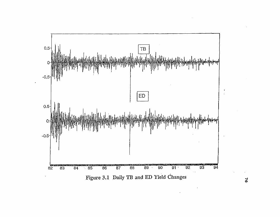
i» iM w n «i n «in iM i iw n»iin » i iiiiiw w i iim n « u i i B»i« ii« iii i i n « i i i n » n i » i i m n iiMi i iuiHuwnu»niiMUr a m » in u ™ ii i — ■ M i i i u u i i a u u n u in i m M l l l l l l B B I l W I I H H I I M I I l lM

8 2 8 3 8 4 8 5 8 6 8 7 8 8 8 9 - 9 0 9 1 • 9 2 9 3 9 4

Figure 3.1 Daily TB and ED Yield Changes

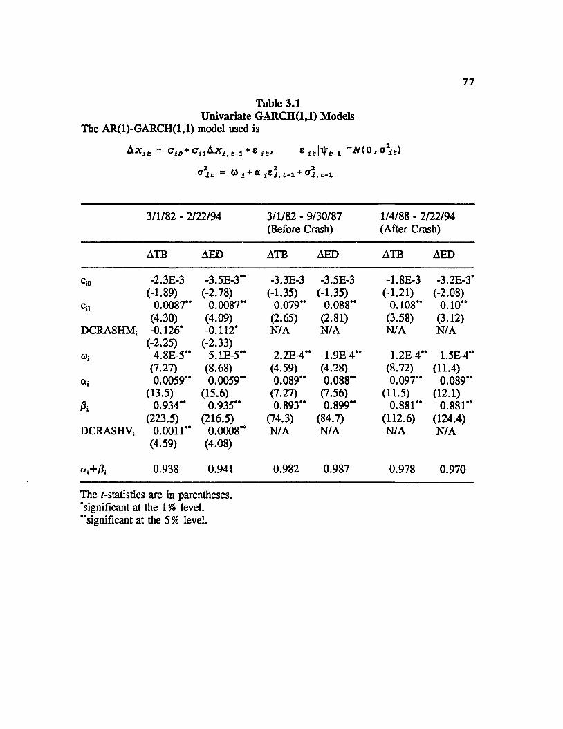
77Table 3.1

Univariate GARCH(1,1) Models The AR(1)-GARCH(1,1) model used is

A x it = cio+ c i A x i.t-i + s it' Sitkt-i ~^(0,a2it)c2it = + +

3/1/82 - 2/22/94 3/1/82 - 9/30/87 (Before Crash)

1/4/88 - 2/22/94 (After Crash)

ATB AED ATB AED ATB AED

Cjo -2.3E-3 -3.5E-3" -3.3E-3 -3.5E-3 -1.8E-3 -3.2E-3*(-1.89) (-2.78) (-1.35) (-1.35) (-1.21) (-2.08)

Cii 0.0087" 0.0087" 0.079’* 0.088" 0.108" 0.10"(4.30) (4.09) (2.65) (2.81) (3.58) (3.12)

DCRASHMi -0.126* -0.112* N/A N/A N/A N/A(-2.25) (-2.33)

OJi 4.8E-5" 5.1E-5" 2.2E-4”’* 1.9E-4" 1.2E-4" 1.5E-4"(7.27) (8.68) (4.59) (4.28) (8.72) (11.4)0.0059" 0.0059" 0.089" 0.088" 0.097" 0.089"

(13.5) (15.6) (7.27) (7.56) (11.5) (12.1)ft 0.934" 0.935" 0.893" 0.899" 0.881" 0.881"

(223.5) (216.5) (74.3) (84.7) (112.6) (124.4)DCRASHVj 0.0011" 0.0008" N/A N/A N/A N/A

(4.59) (4.08)

Ofj+fr 0.938 0.941 0.982 0.987 0.978 0.970

The r-statistics are in parentheses, 'significant at the 1 % level, "significant at the 5% level.

78

Lxit = c JO + cJ1AxJ>t.1 + s Jt, « ~N(0,o2it) (la)o 2lt = w j + a iei,t-i + °i,t-i* (lb)

where xA = TB, or ED,, and \j/t is the information set at time t.For the whole period, dummy variables, DCRASHM and DCRASHV inaccounting for the crash are included in eq. (la) and (lb), respectively.

It shows that the corresponding GARCH parameters of the TB and ED series are very close for each period. Moreover, both series follow a nearly degenerated and integrated GARCH process in each subperiod as indicated by the small (but significant) cjj and the value of a;+/3~=0.98 (but siginificantly different from one) in the variance equation (lb) .2 This estimate of <*;+/?, suggests that the implied half life of a shock to the conditional variance equals In(l/2)/In(0.98) = 34.3 days. As an extreme case, integrated GARCH (otj+/3j=l) introduced by Engle and Bollerslev (1986) implies persistence in shocks to price- or yield-change variance, i.e., a shock to the integrated GARCH volatility process persists for an infinite prediction horizon. This extreme property of the integrated GARCH process does not seem to be consistent with the observed behavior of agents who typically do not frequently and radically change their portfolio compositions,

2Since a dummy variable is added in the variance equation for the whole period, the estimate of may not provide anappropriate analysis on the variance persistence.

and, therefore, many papers have attempted to uncover this persistent movement in variance. Lamoureux and Lastrapes (1990a) demonstrate that this persistence is greatly reduced if any additional information about the variance of the stock- return process after accounting for the rate of information flow, as measured by contemporaneous trading volume.3 However, the value of <*;+& is still close to one (about 0.97) after including the contemporaneous or lagged volume. (Results not reported.) In another context, Diebold (1986) and Lamoureux and Lastrapes (1990b) argue that integrated GARCH may simply be caused by a structural change between, for example, monetary regimes. Since in October 1982, the Federal Reserve returned to interest rate targeting policy from targeting bank reserves, the pre-crash period GARCH model is reestimated starting from 1/2/83. Results show that the value of aj+ft does fall to 0.94 (half-life = 11.2 days). Thus, the persistence in variance may partially induced by the monetary regime shift. Nonetheless, results represented throughout the chapter are qualitatively the same if the whole and the pre-crash periods are estimated from 1/2/83.4

3They even argue that contemporaneous volume is a sufficient statistic for the entire history of squared stock returns in a GARCH specification.

4Baillie, Bollerslev, and Mikkelsen (1993) introduce the new class of Fractionally Integrated Generalized AutoRegressive Conditionally Heteroskedastic (FIGARCH) processes, which implies a slow hyperbolic rate of decay for the influence of shocks to the conditional variance. The FIGARCH process provides a direct analogy to the fractionally

80The above preliminary study may suggest that TB and ED

possess a common volatility process, which can be depicted by a GARCH model. The next section tests this hypothesis by applying a common volatility test.

3.3 Common Volatility

If TB and ED yield changes are found to share a common volatility factor, a factor analytic approach can be applied:

In eq. (2) the yield change is decomposed into two parts: systematic (XiFt) and idiosyncratic (£h) changes. More explicitly, the common factor Ft represents general influences that tend to affect both yields, and the factor loading Xj indicates which yield change is involved in Ft and to what degree; while the £it reflects uncorrelated market-specific shocks. Results (not reported) of a simple factor analysis show that about 97% of variance between TB and ED yield changes is accounted for by Ft, and the ratio of the factor

integrated, or 1(d), class of processes for the conditional mean that is discussed in Chapter 1 Section 1.6. Baillie, Bollerslev and Mikkelsen (1993) and Bollerslev and Mikkelsen (1993), in a univariate analysis, show that the FIGARCH specification is preferable to both the stable GARCH and integrated GARCH models. However, the FIGRACH process in the context of volatility spillover mechanism, a multivariate analysis, is complicated and yet to be developed in the literature.

(2)

81loadings is one to one. Again, these preliminary results seem to suggest that TB and ED share a common volatility factor, and they are equally involved in this factor.

Engle and Kozicki (1993) introduce a class of statistical tests for the hypothesis that some feature that is present in each of the markets is common to them. A common feature is detected by a test that finds linear combinations of returns with no feature. The common feature that is investigated in this chapter is the common volatility process, which is related to the information transmission mechanism.

The common factor is assumed to follow an autogressive conditional heteroscedasticity (ARCH). The common volatility test is used to assess the validity of a simple one-factor ARCH model. Therefore, if TB and ED have a one-factor model representation for yield changes with a time-varying variance, a linear combination of the TB and ED yield changes that does not exhibit time-varying variance can be constructed; i.e., the factor is eliminated. Operationally, testing whether there is a portfolio that has a constant variance exhibiting no ARCH errors (while individual series contains ARCH) is equivalent to testing the validity of the simple model.5

sFor detailed analytical description see Diebold and Nerlove (1989), and Engle and Susmel (1993). Engle and Susmel also point out that if this simple factor model is the true model, more general models may incur overparameterizations and inferences that are inefficient.

The common-feature test has two steps. First, both series are tested for the ARCH feature. Second, if ARCH effects are found in both series, then the test for common ARCH is undertaken. Lagged squared yield changes of order eight are used; results are robust to the orders of four and twelve. Table 3.2 shows that the Langrange multiplier statistics, LM=T*R2, of the univariate-ARCH(8) and multivariate-ARCH(16) (MARCH) tests for both series are significant. The MARCH tests refer to the ARCH test using eight own-market and eight crossmarket lagged squared yield changes. Then the portfolio formed by the linear combination of A^, and A^,, A^, + w x e^t, showing no ARCH is found by iteration of the weight w. Engle and Kozicki (1993) show that the minimum LM is distributed as X2. Panel B shows that the smallest LM in each period is still significant at any conventional levels. Therefore, a single factor does not exist; accordingly, TB and ED do not share the same contemporaneous volatility process, assuming that the common feature follows GARCH.

In sum, the common volatility test gives contradictory results with all of the preliminary results in this and the last sections.

3.4 TED Spread and Volatility Spillovers

3.4.1 Economic Intuition and Preliminary ResultsIn the context of international financial management and

hedging strategies, it is important to understand the extent

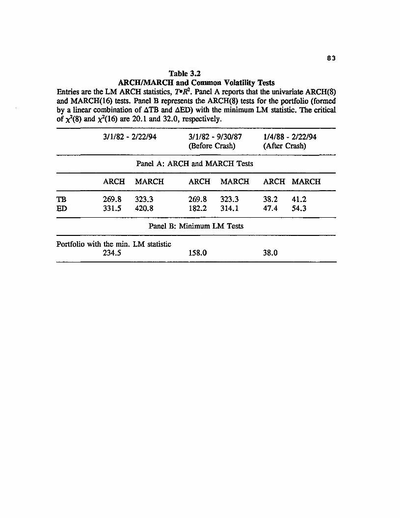
83Table 3.2

ARCH/MARCH and Common Volatility Tests Entries are the LM ARCH statistics, T*R2. Panel A reports that the univariate ARCH(8) and MARCK(16) tests. Panel B represents the ARCH(8) tests for the portfolio (formed by a linear combination of ATB and AED) with the minimum LM statistic. The critical of x2(8) and x2(16) are 20.1 and 32.0, respectively.

3/1/82 - 2/22/94 3/1/82 ■- 9/30/87 1/4/88 - 2/22/94(Before Crash) (After Crash)

Panel A: ARCH and MARCH Tests

ARCH MARCH ARCH MARCH ARCH MARCH

TB 269.8 323.3 269.8 323.3 38.2 41.2ED 331.5 420.8 182.2 314.1 47.4 54.3

Panel B: Minimum LM Tests

Portfolio with the min. LM statistic234.5 158.0 38.0

84to which foreign interest rate shocks impinge upon domestic interest rate. In particular, whether lagged foreign innovation will spillover to the domestic market is of major importance for risk hedging.

Chapter 2 Section 2.3 documents that the TED spread reflects the soundness of the international financial markets. In general, events that jeopardize the economy, especially the soundness of the banking system, tend to widen the spread. A highly volatile TED spread indicates a state of uncertainty; accordingly, if the spread changes substantially on a particular day, TB and ED will also change in either direction in the following day. Moreover, since the spread increases in response to bad economic news, the conditional variance of TB and ED yield changes should be increased more by an increase than by an decrease in the spread.

Table 3.3 supports the notion that the lagged TED spread change squares, (ATEDt.j)2, a proxy for volatility, are related to the current TB and ED yield change squares, (Axit)2. The first three rows of Table 3.3 show that the correlation coefficient between (Axit)2 and (ATEDt.,)2 is not only positively significant, but also higher than between (Ax .,)2 and (Axjlrl)2. Besides, the last row reporting the positive correlation between (Axit)2 and ATED^ evinces the above-mentioned asymmetric volatility influence of the TED spread. It is worth comparing the results of Table 3.3 with those of the common volatility test examined in the last section.

Table 3.3Correlations between the Lag TED Spread Changes and Yield Change Squares

3/1/82 - 2/22/94

ATB,

Ax*

AED,

Corr [(AxJ^Ax^,)2] 0.166 0.122Corr [(Axit)2,(Axj>t.,)2] 0.102 0.162Corr [(Axit)2,(ATEDM)2] 0.319 0.247

Corr [(Axj,)2, | ATED,., | ] 0.296 0.256Corr [(Axit)2,ATEDtrl] 0.138 0.094

All of the Pearson Correlation Coefficients reported are significant at the 1 % level.

86

Indisputably, TB and ED are close substitutes and move in the same direction according to common economic fundamentals during normal economic situations. However, during abnormal environment such as wars, TB and ED may move in an opposite direction and the TED spread becomes wider (narrower) if the situation gets worse (better). During the whole period examined, TB and ED moved in an opposite direction in 195 days; more than 70% of these 195 days happened two weeks before or after the erratic events discussed in Chapter 2 Section 2.3. For example, in January 1991, the eruption of the Persian Gulf War jolted the world's financial markets. Since Eurodollar deposits are only obligations of major commercial banks and are not guaranteed by any government as Treasury bills are, ED yields increased by 29 basis points from 1/2/91 to 1/16/91. During the same period of time, TB yields decreased moderately by nine basis points. That is why the TED spread, which reflects the risk premium of holding a Eurodollar deposit versus a Treasury bill surged in this period. On 1/17/91, speculation that U.S.-led forces were headed for a quick victory convinced some investors that the war would be brief and that there might not be any major damage to Mideast oil facilities. Therefore, on that date, the ED yield fell by 13 points because of the elimination of the war premium that had been established in the market, while the TB yield rose by 14 points as a result of so-called "yield curve trades"— selling short-term bills and using the proceeds

87to buy long-term bonds. (See The Wall Street Journal 1/18/1991.) The TED spread plunged accordingly.

This example demonstrates that during erratic periods, TB and ED respond differently because the risk premium between them dominates economic fundamentals. This explains why TB and ED may not have a common volatility (GARCH) process. Moreover, a significant increase or decrease in the TED spread reveals a state of uncertainty and, therefore, induces volatility to both yields. Evidence showing the effect of TED spread change on the volatility mechanism between TB and ED is presented in the following subsection.

3.4.2 Asymmetric Volatility Model: Bivariate EGARCHWhile the GARCH models describe the volatility clustering

phenomenon, Nelson (1990) contends that they do not discriminate between positive and negative shocks. Black (1976) finds that stock returns are negatively correlated with changes in volatility, a finding which implies that volatility tends to rise when the market declines.

In an attempt to capture the asymmetric impact of innovation on volatility, Nelson (1991) develops the exponential GARCH (EGARCH) model of the form

ln(o2it) = <Pio + q>ii(|Ui.t-il"'Blui.t-il) +0iui.t-i + <Pi*ln(Oi,t_1) , (3)

where uu=xu/au is the standardized residual, and E|uk| = (2/rr)1/2 for conditional normal distributions. He shows that the

asymmetric volatility parameter 6 is significantly negative for modeling the stock market index volatility, suggesting that the variance tends to rise (fall) when the past innovation is negative (positive) in accordance with the empirical evidence for stock returns. From this perspective, 0 should be positive in the current study as an increase in the interest rate corresponds to a decrease in the bond price. The first and second columns of Table 3.4 show that the TB and ED yield changes are individually described well by an AR(1)- EGARCH model. The aforementioned dummy variables accounting for the crash are also included. As expected, the asymmetric volatility parameter 6 is significantly positive. Note that the volatility persistence shown by the parameter <pa eq. (3) is close to one (0.98) , suggesting a shock to the conditional variance is highly persistent.

The volatility spillover mechanism is analyzed by the following bivariate EGARCH model:

A * i t = C i 0 + C i A x i,t-i + c i2A Xj.t-i + e i f t lt ~ N ( Q , o 2it) ( 4 a )

ln(o2it) = <P jo + (|ui< t.-J - E\u±' c_i|) +8 t-i+ <P i ln (<Ji, t_i.)+ ii IA TEDt_x | + 6 i2A TEDt_1 (4b)

ai2.t = P oltC21 + Yi IA TEDt.x | + y2 A TED^ (4c)

A similar GARCH model with no asymmetric volatility has been used by Ng and Pirrong (1994). In the context of industrial metals, they report that the lagged-squared spread has a

89Table 3.4

Univariate EGARCH and Bivariate Volatility Spillover EGARCH Models3/1/82 - 2/22/94

The bivariate volatility spillover AR(1)-EGARCH(1,1) model used is

= C i o + C i A x i.t-i + ci 2 + , e ~ m o , a 2lt)

ln(o2it) = q>i0 + 9 ji(|uJ,e.1|-S|uiit.1|)+0JuJ>t.1 + <pialn(oi#e.1)+ 5 ill A TEDt I + 8 i2 A TEDt.x, u it - e it/ o it

ai2.t = P0lta2t + y1\ATEDt.1\+y^TEDt.lt

Univariate Bivariate

ATB AED ATB AED

<Pio -0.112" -0.098" -0.216" -0.242"(-9.30) (-9.60) (-13.1) (-15.2)

<Pn 0.140" 0.143" 0.100" 0.107"(14.1) (15.3) (13.9) (16.2)

9i 0.093' 0.193" 0.256" 0.297"(1.99) (4.69) (5.00) (6.08)

<Pa 0.977" 0.979" 0.965" 0.961"(409.6) (464.6) (376.3) (384.2)

DCRASHV; 0.363" 0.253" 0.148" 0.06(7.65) (6.17) (4.02) (1.59)

1.56" 1.88" (11.5) (13.6)

* a 0.512" 0.449" (4.39) (4.12)

P 0.918"(347.6)

7 i -1.9E-3"(-3.0)

72 -7.9E-4*(-2.10)

P-Value of Q(12)«it 0.779 0.587 0.803 0.417«h2 0.052 0.408 0.057 0.484Mll«2t 0.259

The f-statistics are in parentheses.'significant at the 5 % level, "significant at the 1 % level.

90significant effect on the variances of both spot and forward returns and on the correlation between these returns.

In the conditional mean eq. (4a) of Axit_it AxiM is added to allow for mean spillover. Note that the lagged TED spread change (or error correction term) is not included in (4a) because it is found to be insignificant in Chapter 2. Nevertheless, including ATED,., in eq. (4a) does not alter the results qualitatively. Concerning the conditional variance equation (4b), the terms | ATED,.! | and SEATED,.! respectively represent the magnitude (symmetric) effect and the sign (asymmetric) effect of the lagged TED spread change. Both £u and Sji should be positive in theory; a change in the TED will increase the volatility of yield changes, and a positive change has a greater impact. Finally, in the conditional correlation eq. (4c), p is the conditional correlation between ATB, and AED, when the TED spread does not change at t-1, i.e., ATED,.!=0. As illustrated by the Gulf War example, the correlation between ATB, and AED, should decline as the lagged TED spread fluctuates greatly (size effect), particularly when it increases (sign effect), a "signal" of instability in the international financial markets. Hence, yl and y2 should be both negative.

Table 3.4 columns 4 and 5 present the results of the EGARCH model. Since the mean spillover parameter cfi is found to be insignificant, results of the conditional mean eq. (4a) are not reported for brevity. Being consistent with the theory

91of asymmetric volatility , for either of the ATBt and AED, conditional variance eq. (4b), <ptl and <pa are significantly negatively at the 1% level. Not surprisingly, p in eq. (4c) is 0.91 and significant at any conventional levels due to the fact that TB and ED yields are moving in response to the same fundamentals except during erratic events. Also, as presumed, 7, and y2 are significantly negative, though the latter is only marginally significant at the 5% level. The diagnostic checking of the residuals provides little evidence of misspecif ication; the Ljung-Box Q-statistics of the standardized residuals, uht and their squares, and the cross product standardized residuals uitujt are all insignificant.

Therefore, the volatility spillover mechanism between markets is well described by the bivariate EGARCH model, which shows that the lagged TED change is the driving factor for the volatility process. In particular, a large lagged change of the spread suggests a state of uncertainty as reflected by a higher conditional variance of yield changes, and, consequently, implies an increase in risk premium of Treasury bills over Eurodollar deposits. These influences are greater when the change is positive than when it is negative.

The pre- and post-crash periods are also examined by the same model. In general, results shown in Table 3.5 are similar to those of Table 3.4; except in the conditional correlation equation (4c), the volatility impacts, both symmetric and asymmetric, of the TED spread change for the pre-crash period

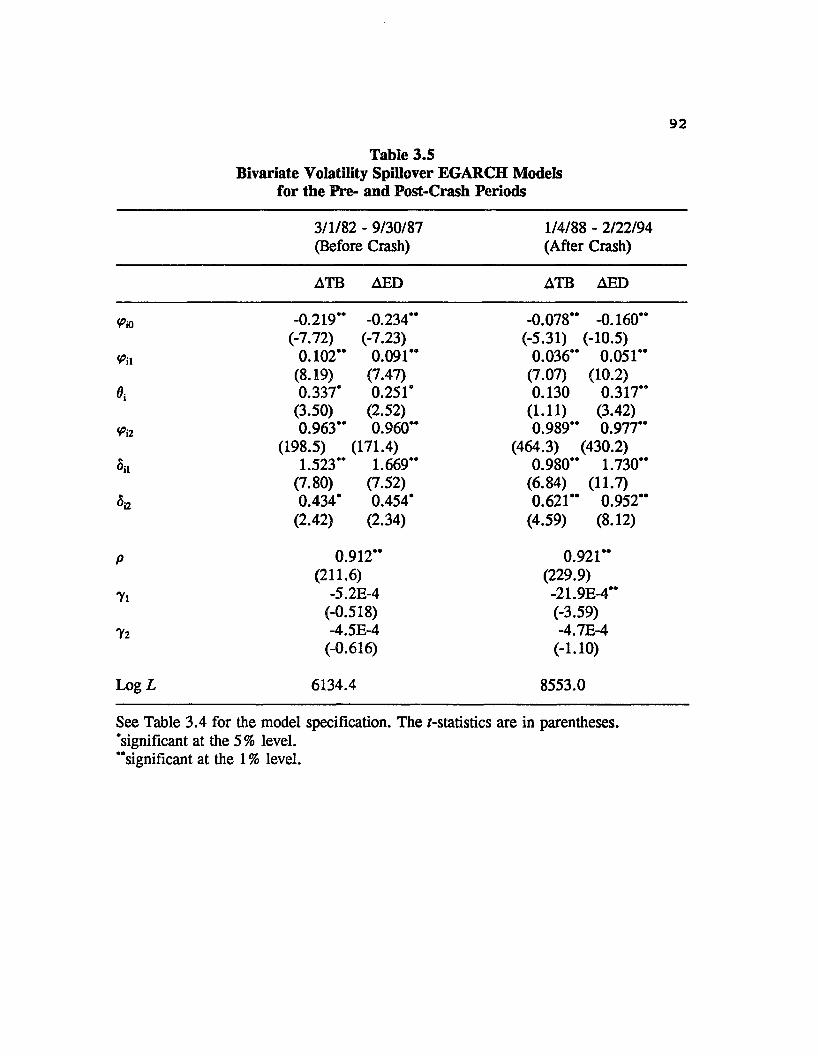
92Table 3.5

Bivariate Volatility Spillover EGARCH Models for the Pre- and Post-Crash Periods

3/1/82 - 9/30/87 1/4/88 - 2/22/94(Before Crash) (After Crash)

ATB AED ATB AED

<Pn -0.219“ -0.234“ -0.078“ -0.160**(-7.72) (-7.23) (-5.31) (-10.5)

<Pn 0.102“ 0.091“ 0.036“ 0.051“(8.19) (7.47) (7.07) (10.2)

Oi 0.337* 0.251* 0.130 0.317“(3.50) (2.52) (1.11) (3.42)

<Pa 0.963** 0.960“ 0.989** 0.977**(198.5) (171.4) (464.3) (430.2)

1.523“ 1.669“ 0.980“ 1.730“(7.80) (7.52) (6.84) (11.7)

5i2 0.434* 0.454* 0.621“ 0.952“(2.42) (2.34) (4.59) (8.12)

P 0.912“ 0.921“(211.6) (229.9)

7i -5.2E-4 -21.9E-4**(-0.518) (-3.59)

72 -4.5E-4 -4.7E-4(-0.616) (-1.10)

Log L 6134.4 8553.0

See Table 3.4 for the model specification. The /-statistics are in parentheses, ‘significant at the 5% level.“significant at the 1 % level.

93and that of the asymmetric volatility effects for the postcrash period are insignificant at the 5% level. The signs of these parameters (7, and y2), however, are still negative, consistent with the theory.

3.4.3 Comparison of Alternative Volatility Spillover ModelsWhile the last subsection shows that the bivariate EGARCH

models provides evidence consistent with the theory, it is worthwhile to examine alternative models (with the conditional mean equations remain unchanged) for the volatility spillover mechanism, particularly the widely used GARCH(1,1) model, e.g., Hamao et at. (1990), denoted Model A in Table 3.6 as follows.

o2it = o i + a Je3.t-i + P Jo?.t_1 + ic1e5.t-i, aijit = pa ita jt (5)

Note that the TED spread is not incorporated into Model A. The symmetric cross-market volatility spillover, from market j to market i, is elicited by the term

The more recent subperiod, the post-crash period, is used in this subsection. Tables 3.6 demonstrates that is insignificant in the ATB equation, but significant in the AED equation. These results suggest a unidirectional volatility spillover from ATB to AED. However, when the term 6a(ATED,.|)2 is added into eq. (5): Model B, the direction reverses and k, becomes negative (-0.005 and -0.001 in the ATB and AED equations, respectively). Most importantly, Sa is each

94Table 3.6

Alternative Volatility Spillover Models for the Post-Crash Period (1/4/88-2/22/94) Model A, GARCH with cross-market spillovers:

ait = w i + ai8i, t-l + Pici, fc-1 t-1* = P ® i t a jt

Model B, GARCH with cross-market and TED change squares spillovers:

a \ t = 0>i + j, t-1+ Pi°i. t-i + t-i + CijA TEDI-x

Q lj, t = + YiATfiDt-i

Model C, GARCH with cross-market and asymmetric TED change squares spillovers:

Q±t - <i) j +ffj£ j, t-i + Pi^i, t-i t-i \TEDf-_i | +6izATEDf..!

Model

(A)ATB AED

(B)ATB AED

(QATB AED

“M i 1.5E-4" 1.6E-4" 9.1E-5" 1.1E-4" -3.9E-5"-4.3E-5"“M i 0.120" 0.100" 0.009" 0.004" 0.007" 0.003"N<Pa 0.851" 0.847" 0.871" 0.862" 0.856" 0.856"K 0.010 0.033" -0.005" -0.001 -0.004" -0.0015ii 0.410" 0.458" 0.003" 0.003"Su 3.8E-3* 7.6E-3"p 0.899" 0.927" 0.919"7i -0.007" -1.4E-3*72 -1.1E-3*

Log L 8294.6 8445.4 8460.4

Note that the /-statistics are not shown for brevity, ‘significant at the 5 % level, "significant at the 5 % level.

95variance equation is positively and highly significant, and its value (about 0.4 in each equation) is much larger than kt. Results of Models A and B illustrate that the volatility spillovers from TED changes is dominating those from the cross-market volatility, a finding that is consistent with the correlation results reported in Table 3.3. This proposition is further supported by the fact that the log maximum likelihood value (Log L) of Model B is greater than Model A by 150.8 (with a p-value<0.001). Then the asymmetric volatility effect of the TED spread change is examined by replacing the symmetric volatility term (ATED^)2 with £u | ATEDU | and S^ATED^ as in Model C. Being consistent with the EGARCH results, both Sa are Sa positive and significant; however, the constant term Wj is negative. Note the Log L of the EGARCH model (8496.7) used in the last subsection for the post-crash period is greater than any of these three GARCH models.

The overall results reinforce the argument that the TED spread volatility spillovers play an important role in the spillover mechanism; ignoring the TED spread in the model may give biased results.

3.5 Conclusions

Using U.S. Treasury bill and Eurodollar futures daily data, this chapter analyzes the causal relationship via the second moment, i.e., the volatility spillovers, between U.S. and Eurodollar interest rates. The GARCH-type models are shown

to well model the volatility processes of both yield changes. Although some preliminary statistics seem to support the hypothesis that TB and ED share the same volatility process, which follows a GARCH process, this hypothesis is rejected by the common volatility test of Engle and Kozicki (1993). A further examination indicates that during erratic periods, TB and ED responds differently (even moving in opposite directions) because the risk premium between them dominates economic fundamentals.

A bivariate exponential GARCH (EGARCH) model which allows for asymmetric volatility influence of the TED spread, as well as that of the domestic market, is used to model the volatility spillovers between markets. The model shows that the lagged TED spread change is the driving force of the volatility process, a finding that is robust to the pre- and post-crash period examination. The reason is that, when the TED spread is highly volatile, the financial market is in a state of uncertainty, and, accordingly, the (conditional) variance of interest rates increases. In particular, a large lagged change of the spread implies an increase in risk premium of Treasury bills over Eurodollar deposits. These influences are greater when the change is positive than when it is negative, suggesting asymmetric volatility spillovers from the TED spread changes.

CHAPTER 4

THE INTERNATIONAL TRANSMISSION OF INFORMATION IN EURODOLLAR FUTURES MARKETS

4.1 Introduction

Eurodollar futures are now the most actively traded short-term interest rate futures contracts. This chapter investigates the international transmission mechanism in three Eurodollar futures markets in the Chicago, Singapore, and London exchanges. A better understanding of the transmission mechanism may provide investors with more efficient strategies for hedging or speculating interest rate risk associated with Eurodollar deposits.

A Eurodollar futures contract calls for the delivery (cash settlement) of a $1 million, 3-month, Eurodollar time deposit. Eurodollar futures were introduced in December 1981, by the IMM (International Monetary Market, a division of the Chicago Mercantile Exchange (CME)) in Chicago. Eurodollar futures provide a way that banks can hedge the interest rate risk associated with Eurodollar deposits, on which major international corporations have come to rely increasingly.

Eurodollar futures (hereafter, ED, the ticker symbol) started trading in Singapore, SIMEX, (Singapore International Monetary Exchange) and London, LIFFE, (London International Financial Futures Exchange) in September 1982 and September

97

981984, respectively, and therefore can be traded on a global, 24 hour, basis.1 In Chicago time, SIMEX opens from 7:30 p.m. to 4:20 a.m., the LIFFE opens from 2:30 a.m. to 10 a.m., andthe IMM opens from 7:20 a.m. to 2:00 p.m. (See Table 4.2 forthe numbers of trading and nontrading hours.) Figure 4. la depicts each trading period, and Figure 4.1b describes three possible orderings of the trading sequence within 24 hours. The importance of the latter is realized in Sections 4.5 and 4.6. The 1990 annual trading volume of ED traded at the IMM was 34.7 million contracts, and was about 10 times that traded on the SIMEX and 20 times that traded on the LIFFE. Theinterrelationship between the IMM and SIMEX is further strengthened by the mutual offset arrangement between them.2

Comparing the trading and nontrading time variances, the IMM and LIFFE markets are found to be more volatile when they are trading. In contrast, the Singapore market is morevolatile when it is closed. These results suggest that relevant information reveals more during the trading hours of the IMM market than those of the SIMEX market. Yields implied in the three markets are shown to be cointegrated with a single stochastic trend. The impulse responses and the fractions of forecast error variances in each market

•Eurodollar futures traded in Tokyo (TIFFE), which is introduced in October 1990, are not considered in the paper because of the insufficient trading history.

2The mutual offset arrangement means that Eurodollar futures positions established at the IMM may be offset at the SIMEX, and vice versa.

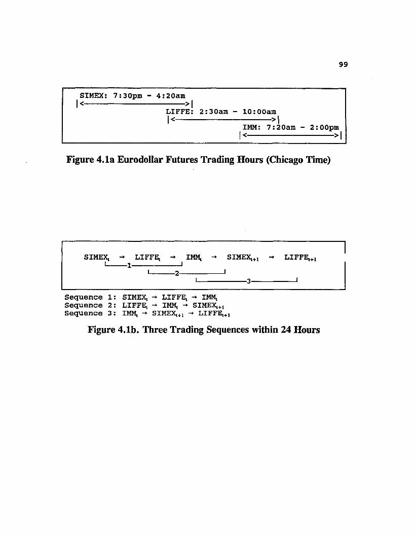
99

SIMEX: 7:30pm - 4:20am|<---------------------- >|LIFFE: 2:30am - 10:00aml<---- ----------------- >|

IMM: 7:20am - 2 :00pm|<-------------- ------>1

Figure 4.1a Eurodollar Futures Trading Hours (Chicago Time)

SIMEX, -* LIFFE, -+ IMM, -► SIMEX,+1 -» LIFFE,+1 I 1 --------- 1

Sequence 1: SIMEX, - LIFFE, -> IMM,Sequence 2: LIFFE, -*• IMM, SIMEX,+1 Sequence 3: IMM, -*• SIMEX,+1 -*• LIFFE,+1

Figure 4.1b. Three Trading Sequences within 24 Hours

100

attributed to the common stochastic trend are computed. Employing an approach that explores this common factor and allowing for the nonsynchronous trading problem among markets, this chapter provides evidence that the market is extremely efficient on a daily basis. The responses of all markets to an innovation to the common factor are fully settled within a day. Lastly, the significant results of volatility spillovers among markets suggest that certain market dynamics lead to a continuation of volatility. Particularly, the volatility spillover mechanism may be influenced by the US stock markets.

The following section discusses the data and presents the summary statistics. Section 4.3 examines the trading and nontrading time variance of yield changes. Section 4.4 analyzes the transmission mechanism among markets by employing cointegration methodology. The causality relationship is studied in Section 4.5. Using the results in Section 4.4 and identifying the common stochastic trend, Section 4.6 investigates the variance decomposition and impulse response functions. Results of volatility spillovers are reported in Section 4.7. The last section concludes the chapter.

4.2 Data and Summary Statistics

Daily open and close index prices for the period after the October 1987 stock market crash— January 4, 1988 toFebruary 22, 1994 (1585 observations)— are collected fromCommodity Systems, Inc. (CSI). Several studies report that

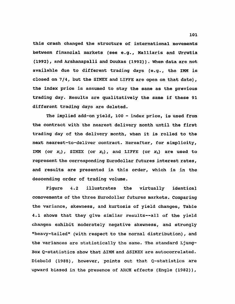
101

this crash changed the structure of international movements between financial markets (see e.g., Malliaris and Urrutia (1992), and Arshanapalli and Doukas (1992)). When data are not available due to different trading days (e.g., the IMM is closed on 7/4, but the SIMEX and LIFFE are open on that date), the index price is assumed to stay the same as the previous trading day. Results are qualitatively the same if these 91 different trading days are deleted.

The implied add-on yield, 100 - index price, is used from the contract with the nearest delivery month until the first trading day of the delivery month, when it is rolled to the next nearest-to-deliver contract. Hereafter, for simplicity, IMM (or x,), SIMEX (or x2), and LIFFE (or x3) are used to represent the corresponding Eurodollar futures interest rates, and results are presented in this order, which is in the descending order of trading volume.

Figure 4.2 illustrates the virtually identical comovements of the three Eurodollar futures markets. Comparing the variance, skewness, and kurtosis of yield changes, Table4.1 shows that they give similar results— all of the yield changes exhibit moderately negative skewness, and strongly "heavy-tailed” (with respect to the normal distribution), and the variances are statistically the same. The standard Ljung- Box Q-statistics show that AIMM and ASIMEX are autocorrelated. Diebold (1988), however, points out that Q-statistics are upward biased in the presence of ARCH effects (Engle (1982)),

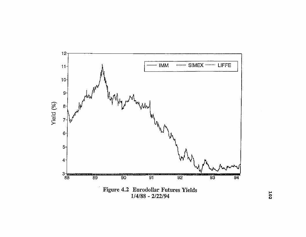
Yield

(%

)12

SIMEX LIFFEIMM

IQ-

91 9 2 9 3 9 488 8 9 9 0

Figure 4.2 Eurodollar Futures Yields 1/4/88 - 2/22/94

102

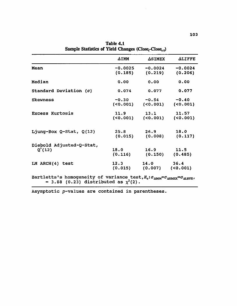
103Table 4.1

Sample Statistics of Yield Changes (Closet-Closeti)

AIMM ASIMEX ALIFFEMean -0.0025

(0.185)-0.0024(0.219)

-0.0024(0.206)

Median 0.00 0.00 0.00Standard Deviation (a) 0.074 0.077 0.077Skewness -0.30

(<0.001) -0.54(C0.001) -0.40

(<0.001)Excess Kurtosis 11.9

(<0.001)13.1(<0.001)

11.57(<0.001)

Ljung-Box Q-Stat, Q(12) 25.8(0.015)

26.9(0.008)

18.0(0.117)

Diebold Adjusted-Q-Stat, Q*(12) 18.0

(0.116)16.9(0.150)

11.5(0.485)

LM ARCH(4) test 12.3(0.015)

14.0(0.007)

36.4(<0.001)

Bartletts's homogeneity of variance test, Hn: aAiMi gaiimfy Jatipbb, = 3.88 (0.23) distributed as x2(2).

Asymptotic p-values are contained in parentheses.

104which are indicated by the Langrange multiplier ARCH tests. Using Diebold's ARCH-adjusted Q* test, all yield changes are then shown to be serially uncorrelated.3 Together with insignificant means, the statistics suggest a martingale process with GARCH (Bollerslev (1986)) innovations in the Eurodollar futures markets.

4.3 Volatility During Trading and Nontrading Hours

Empirical studies that focus only on the trading and nontrading periods of the U.S. security market fail to properly address the question of the effect of open markets in other countries on the time pattern of risk for those assets which are traded internationally. Hill and Schneeweis (1990) examine the trading to nontrading variance of the Treasury bond futures and Eurodollar for July and August from 1986 and 1988. They find that variances of price changes differ both between trading and nontrading hours and between the trading hours of different markets: variances during trading periods seem to be greatest for those markets which are open when the information flow occurs.

Koh and Tsui (1992) examine ED contracts for the period 1982 to 1989. While their results are generally consistent with Hill and Schneeweis (1990) , they point out that ED prices

3Lo and MacKinlay's (1988) variance ratio test, which is heteroskedasticity-consistent (including ARCH), also give no evidence of serial correlation.

105are more volatile during exchange trading hours than nontrading hours on the IMM and the LIFFE, but not on the SIMEX. They suggest that, from a trading-strategy point of view, the times of greatest volatility, which are what speculators look for, take place during Chicago trading hours and the times of lowest volatility, which are what hedgers look for, take place during Singapore trading hours.

The current study updates the results of Hill and Schneeweis (1990) and Koh and Tsui (1992) for the post-crash period. In stock markets, Arshanapalli and Doukas (1993), among others, show that the degree of international linkage among stock price indices has increased substantially. If this is also the case for the Eurodollar markets, it might be expected that the difference of volatility between trading and nontrading hours decreases after the crash.

4.3.1 Empirical Results4Table 4.2 Panel A demonstrates that the trading time

(open-to-close) variances per hour, o2y , are very different among these three markets, with AIMM being the greatest and ASIMEX being the smallest. Note that o2y of ASIMEX is six times less than ALIFFE, though the trading volume of the former istwice higher. In contrast, in Panel B, the Singapore market

4For simplicity, the results reported do not consider the effects of weekends and holidays. Results are qualitatively the same when these effects are taken into account, and are available upon request.

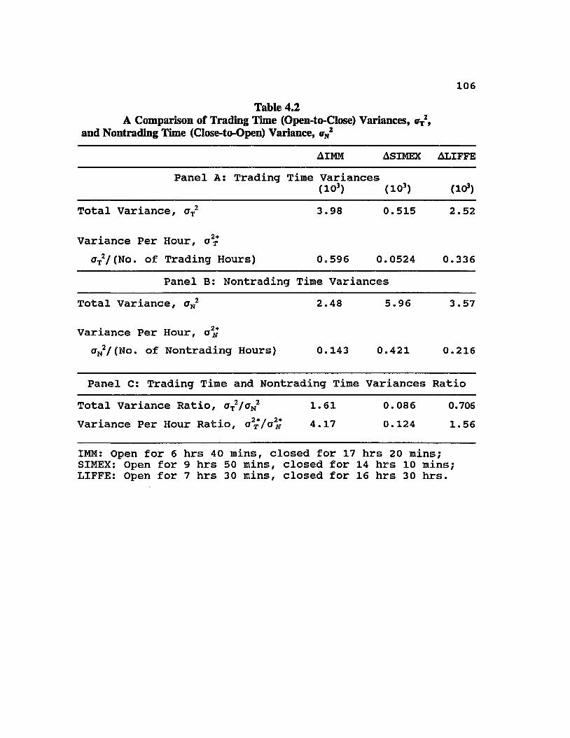
106Table 4.2

A Comparison of Trading Time (Open-to-Close) Variances, <rT2, and Nontrading Time (Close-to-Open) Variance, <rN2

AIMM ASIMEX ALIFFEPanel A: Trading Time Variances

(103) (103) (103)Total Variance, 0X2 3.98 0.515 2.52

Variance Per Hour, o2?

°tV(N o . of Trading Hours) 0.596 0.0524 0.336Panel B: Nontrading Time Variances

Total Variance, ctn2 2.48 5.96 3.57

Variance Per Hour,aN2/ (No. of Nontrading Hours) 0.143 0.421 0.216

Panel C: Trading Time and Nontrading Time Variances RatioTotal Variance Ratio, 0T2/aN2 1.61 0.086 0.706Variance Per Hour Ratio, o2x/a^ 4.17 0.124 1.56

IMM: Open for 6 hrs 40 mins, closed for 17 hrs 20 mins; SIMEX: Open for 9 hrs 50 mins, closed for 14 hrs 10 mins; LIFFE: Open for 7 hrs 30 mins, closed for 16 hrs 30 hrs.

107gives the greatest nontrading time (close-to-open) variances per hour, The per hour trading and nontrading time

variance ratios, ct / ct , are presented in Panel C. It shows that the trading time variances are greater than the nontrading time variances in the U.S. and London markets with the ratios of 4.17 and 1.56, respectively; but the opposite is true for the Singapore market with a ratio of 0.124.

The results are in general consistent with Hill and Schneeweis (1990) and Koh and Tsui (1992) . The different result of the Singapore market from the other two markets may be explained by the information hypothesis that volatility changes in response to the arrival and assimilation of public information that is not uniform across trading and nontrading hours5. That is, Eurodollar interest rates are driven by the economic information concerning the U.S. and European countries that is revealed in Chicago and London times. Moreover, Fung and Leung (1993) find that the Eurodollar cash and futures markets are cointegrated and bidirectionally Granger-cause each other. These active US and European cash markets are open during the nontrading hours of the Singapore markets.

5If yield change volatility is mainly derived from noise trading, the volatility is related to trading activities when the markets are open. However, if volatility is caused by the release of public information, volatilities during trading and nontrading hours are only related to the information flow instead of trading activities. See French and Roll (1986) , Ross (1989), and Barclay, Litzenberger, and Warner (1990) for more information.

108Furthermore, two non-exclusive reasons can explain the

higher trading/nontrading variance of the U.S. market than the London market. First, the trading volume at the IMM dominates that at the LIFFE. Second, the Eurodollar interest rates are closely related to the U.S. domestic interest rate; namely, the Treasury bill. Specifically, trading the interest rate differential between Eurodollar and Treasury bill futures, the TED spread, can be a means to speculate on general economic conditions and on the soundness of banks in particular without incurring interest rate risk. In general, events that jeopardize the soundness of the banking system tend to widen the spread. (See Chapter 2, Section 2.3 for detailed description on this issue.)

4.4 Unit Root and Cointegration

Unit root tests in Table 4.3 indicate that IMM,, SIMEX,, and LIFFE, can be characterized as 1(1) processes according to the augmented Dickey-Fuller (ADF) tests (Dickey and Fuller (1979, 1981) and the Phillips-Perron (PP) tests (Phillips(1987), and Phillips and Perron (1988)).

Let X, = (xlt xa x3t) '; N = the number of variables in the system, three in this case. If X, is cointegrated, it can be generated by a vector error correction model (VECM) :

A X t = H + A lA X t_1 + “ ' + A k _ 1 & X t _ k _ 1 + A k X c _ 1 + C t m

where A's are 3x3 matrices of parameters, e, is a 3x1 vector

109Table 4.3

Augmented Dickey-Fuller and Fhillips-Perron Unit Root Tests ADF and PP denote the augmented Dickey-Fuller test and the Phillips-Perron test statistics, respectively. ADF1 and PP1 are computed with a constant term; and ADF2 and PP2 are with a constant and a linear trend. The statistics are computed with 10 lags for the ADF tests and 10 non-zero autocovariances in Newey-West (1987) correction. Results are robust for 5, 20, and 30 lags— the hypothesis that a unit root in each series is not rejected. The critical values for both statistics, which are asymptotically equivalent, are available in Fuller (1976, p.373) .

IMM SIMEX LIFFEADF1ADF2

-0.200 -0.237 -0.250-2.264 -2.350 -2.270

PP1PP2

-0.235 -0.239 -0.257-2.264 -2.352 -2.276

110

white noise. The Johansen trace test statistic of the hypothesis H0:r=r0 against Bim.r>r0, with r being the cointegrating rank, is

-2lnQ = -(T-Nk) V lnd-Xj),i-x0*l

where Xj's are the N-r0 smallest squared canonical correlations of X^ with respect to AXt corrected for lagged differences and T is the sample size actually used for estimation. Reinsel and Ahn (1992) find that the Johansen tests over-reject when the null is true, and suggest correcting this using (T-Nk) instead of T as shown in the above form. The Johansen maximum eigenvalue (\„„) test statistic of the hypothesis H0: r=r„ against H1: r=r0+l is

*max = -(T-Nk)ln(l-XTo+1) ,(3)

where £ro+1 is the (r„+l)th greatest squared canonical correlation.

Table 4.4 Panel A shows that the lag length k in the VECM (1) chosen by the Akaike and Schwarz information criteria (AIC and SIC) are 4 and 2, respectively. Reimers (1991) finds that the SIC does well in selecting k. However, since the role of the lagged differences of Xt in the VECM is to whiten the error et, it is not certain that the SIC will select k=2 so that e, is white. Hence residual diagnostics for the estimated model using the k selected by the SIC are examined. In Panel B the

I l l

Table 4.4VECM Specification and Johansen Cointegration Tests

Xt = (xlt x* x3t)', and the VECM isL X t = \l +A1kXt_1 + '“+Ak_1AXt_k_1 + AkX t_1 + e t

Panel A: Lag Selection in VECM*k=2 k=3 *=4 k=5

AIC -18.59 -18.60 -18.61 -18.60SIC -18.53 -18.50 -18.48 -18.44

Panel B: Residual Diagnostics’*IMM SIMEX LIFFE

Ljung-Box test 0.292 0.734 0.055Skewness test <0.001 <0.001 <0.001Excess kurtosis test <0.001 <0.001 <0.001

Panel C: Johansen Cointegration Tests'Trace

m=l 0.0606 0.0606m=2 658.5“ 658.42“m=3 1457.1“ 798.6“‘For Panel A,

AIC = ln|ErJ + 2g/r; and SIC = ln|£t>w| + gln(T)/T,

where Zr>N denotes the Johansen ML estimate of the residual covariance matrix Z£ and q=N2 (k-1) +N+2Nr-rl is the number of freely estimated parameters of the VECM because r2 restrictions are used in Johansen ML procedure. bFor Panel B, p-values are reported.'For Panel C, m=N-r is the number of common trends. The critical values are obtained from Osterwald-Lenum (1992). Results reported for k=2 are qualitatively the same for k~3, 4, and 5.“significant at the 1% level.

1 1 2

asymptotic p-values for the Ljung-Box test for up to the 20th order serial correlation in the residuals indicate that the serial correlation is insignificant for all equations in the system.6 The results reported in this chapter are qualitatively the same for k=4, the lag chosen by AIC.

The results of the Johansen (1991) cointegration tests are reported in Panel C. It demonstrates that the interest rates implied in the futures contract of the three futures markets are cointegrated with r=2. To ensure that this cointegration result is not biased by nonsynchronous trading problem among the three markets, the Johansen tests are conducted for the following two adjusted data sets: (1) oneday lag of IMM; (2) one day lags of IMM and LIFFE. (The nonsynchronous problem is discussed in the next two sections.) The cointegration results remain unchanged.

4.5 Granger Causality Among Markets

To examine the directions of causation in the Granger sense among the yield changes of three markets, the following error correction model— Model A— is estimated:

‘‘Moderate skewness and strongly excess kurtosis are found in all equations. As the Johansen tests are constructed under the Gaussian assumption, Cheung and Lai (1993b) examine the bias in the size of the Johansen tests due to non-normal innovations, including non-symmetric and leptokurtic ones. They find that both the trace test and test are reasonably robust.

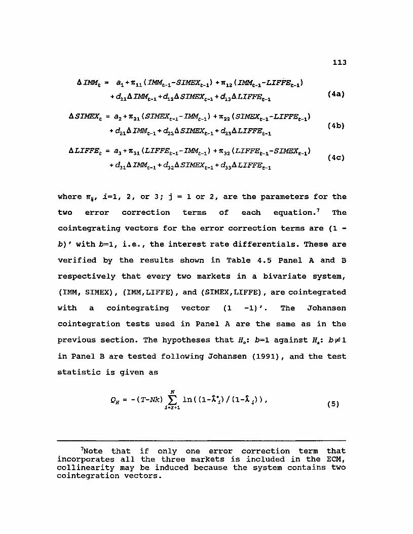
113

A IMMt = ax + Itn (IMMt_ x - SIMEXt_ x) + 1I12 (IMM^-LIFFE^) + dxlA +d12ASIMEXt_1 + du ALIFFEt.x (4a)

A SIMEX,. = a2 + IC21 (SIMEXt_x-IMMt_J + w22 ( SIMEXt_2-LIFFEt_2) + d ^ A l M M ^ + d^ASIMEX^ + d 3 A LIFFEt-1 (4b)

; a3 + *31 (LIFFE^-IMM^) + W32 (LIFFEt_x-SIMEXt_2) + d„AlMMt_, +d„ASIMEXt._,+d„ALIFFEf._,

where w-, 1=1, 2, or 3; j = 1 or 2, are the parameters for thetwo error correction terms of each equation.7 Thecointegrating vectors for the error correction terms are (1 - b)' with Jb=l, i.e., the interest rate differentials. These are verified by the results shown in Table 4.5 Panel A and B respectively that every two markets in a bivariate system, (IMM, SIMEX), (IMM,LIFFE), and (SIMEX,LIFFE), are cointegrated with a cointegrating vector (1 -1)'. The Johansencointegration tests used in Panel A are the same as in theprevious section. The hypotheses that HQ% b=l against Htm. b ^ l in Panel B are tested following Johansen (1991), and the test statistic is given as

7Note that if only one error correction term that incorporates all the three markets is included in the ECM, collinearity may be induced because the system contains two cointegration vectors.

NQh = - (T-Nk) Y, ln((l-£i>/(!-£*)) (5)

114Table 4.5

Johansen Tests and Cointegrating Vectors for Bivariate Systems*

(IMM, SIMEX) (IMM,LIFFE) (SIMEX,LIFFE)Panel A: Johansen Tests

Tracem=l 1564.5" 759.5" 875.4"m=2 0.05 0.06 0.04m=l 1564.0" 759.5" 875.3"m=2 0.05 0.06 0.04

Panel B: Cointegrating Vectors, (1 -b) 'b 0.99 1.00 0.99p-value of H0:b=l (0.99) (0.99) (0.99)•Results reported for k=2 in the VECM are qualitatively the same for k=3, 4, and 5."significant at the 1% level.

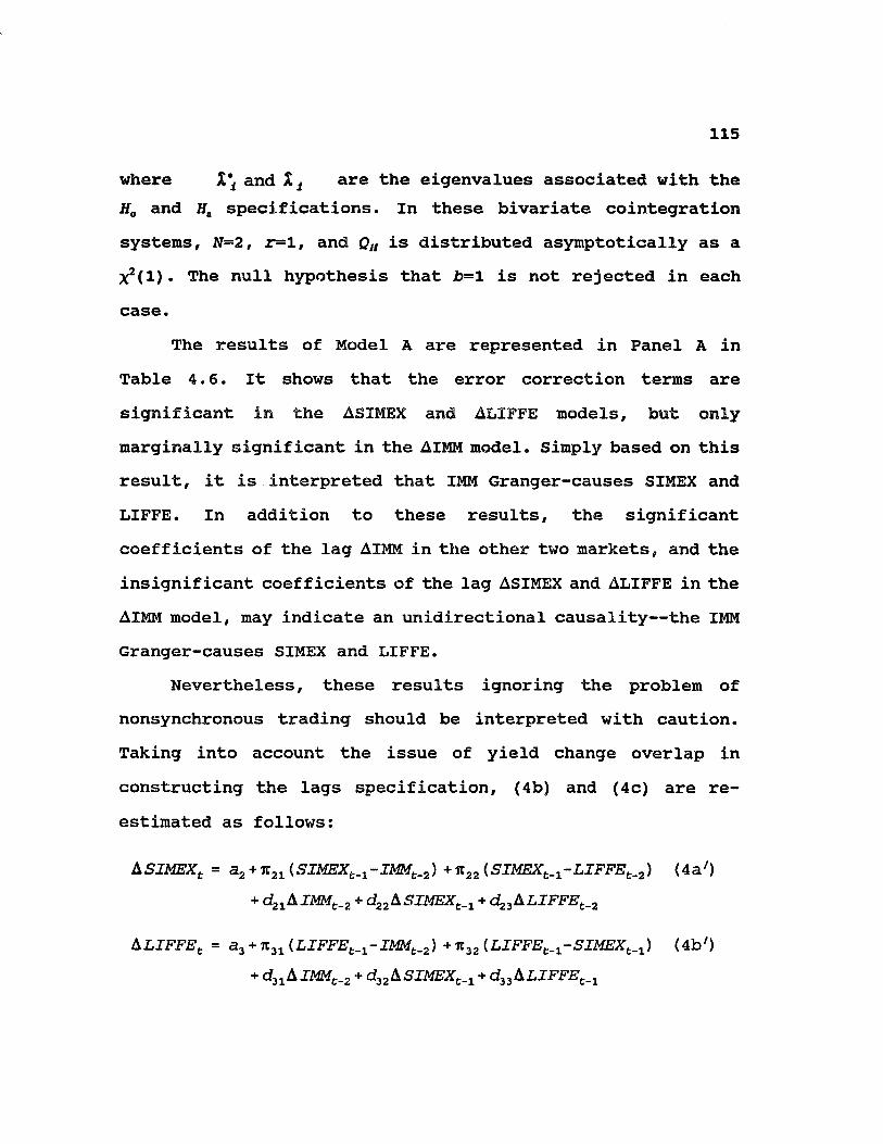
115

where X\ and X ± are the eigenvalues associated with the Ha and Ha specifications. In these bivariate cointegrationsystems, N=2, r=1, and Q„ is distributed asymptotically as aX2(l). The null hypothesis that Jb=l is not rejected in eachcase.

The results of Model A are represented in Panel A in Table 4.6. It shows that the error correction terms are significant in the ASIMEX and ALIFFE models, but only marginally significant in the AIMM model. Simply based on this result, it is interpreted that IMM Granger-causes SIMEX and LIFFE. In addition to these results, the significant coefficients of the lag AIMM in the other two markets, and the insignificant coefficients of the lag ASIMEX and ALIFFE in the AIMM model, may indicate an unidirectional causality— the IMM Granger-causes SIMEX and LIFFE.

Nevertheless, these results ignoring the problem of nonsynchronous trading should be interpreted with caution. Taking into account the issue of yield change overlap in constructing the lags specification, (4b) and (4c) are re-estimated as follows:

ASIMEXt = a2 + rc21 (SIMEXt_x-IMMt_2) + n22 (SIMEXt_3-LIFFEt_2) (4a')+ d21AlMMt_2 + d22ASIMEXt.x + d23ALIFFEt_2

A LIFFE t = a3 + n31 (LIFFE^-IMMt_2) + it32 (LIFFEt.x-SIMEXt-1) (4b')+ d31AlMMc_2 + d32 A SIMEXt_x + d33 A LIFFE

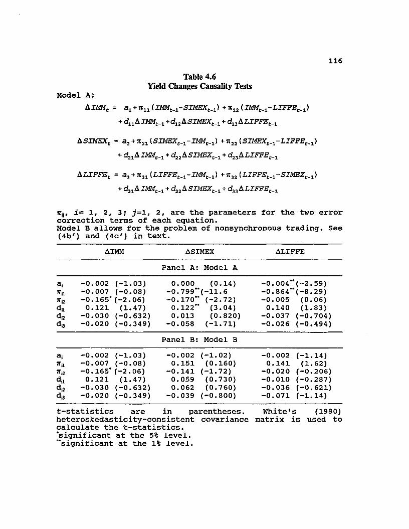
116Table 4.6

Yield Changes Causality TestsModel A:

AlMMt = ax + 71 lx (IMMt_x-SIMEXt_x) +x12(IMMt_1-LIFFEt_1)+ dxxAlMMt.x +d12 A SIMEXt_x + d13 A LIFFEt_x

ASIMEXt = a2 + 7l21 (SIMEXt.x-IMMt.x) + n22{SIMEXt_x-LIFFEt_x)+ d^A JAZMfc.i + d 2 A SIMEXt_x + d23ALIFFEt.x

ALIFFEt = a3 + n31{LIFFEt_x-IMMt.x) + ir32 (LIFFEt.x-SIMEXt_x)+ d31 A IMMt_x + d32ASIMEXt_x + d33ALIFFEt_x

TTy, i= 1, 2, 3; j=l, 2, are the parameters for the two error correction terms of each equation.Model B allows for the problem of nonsynchronous trading. See (4b') and (4c#) in text.

AIMM ASIMEX ALIFFEPanel A: Model A

ai -0.002 (-1.03) 0.000 (0.14) -0.004“ (-2.59)tf.t -0.007 (-0.08) -0.799“ (-11.6 -0.864“ (-8.29)

-0.165* (-2.06) -0.170“ (-2.72) -0.005 (0.06)di, 0.121 (1.47) 0.122“ (3.04) 0.140 (1.83)d,7 -0.030 (-0.632) 0.013 (0.820) -0.037 (-0.704)d3 -0.020 (-0.349) -0.058 (-1.71) —0.026 (-0.494)

Panel B: Model Bai -0.002 (-1.03) -0.002 (-1.02) -0.002 (-1.14)ii -0.007 (-0.08) 0.151 (0.160) 0.141 (1.62)

-0.165’(-2.06) -0.141 (-1.72) -0.020 (-0.206)di, 0.121 (1.47) 0.059 (0.730) -0.010 (-0.287)dra -0.030 (-0.632) 0.062 (0.760) -0.036 (-0.621)dB -0.020 (-0.349) -0.039 (-0.800) -0.071 (-1.14)t-statistics are in parentheses. White' S (1980)heteroskedasticity-consistent covariance matrix is used to calculate the t-statistics.‘significant at the 5% level.“significant at the 1% level.

117The difference between the above error correction model, Model B, and Model A is: the IMM yields and yield changes are given a two-day lag in the SIMEX (4b') and LIFFE (4c') markets; the LIFFE yields and yield changes are given to a two-day lag in the SIMEX market.

In contrast to Model A, Model B gives no significant results of the error correction terms or cross-market lagged yield changes in the SIMEX and LIFFE models. Taken together, results of Model A and Model B indicate that causality possibly runs from the IMM market but this causal relationship is shorter than one day. The question of which market is dominant in the context of information transmission is elicited more clearly in the next section.

4.6 Variance Decomposition and Impulse Response Analysis

Since Sims (1980), variance decomposition and impulse response analysis based on VAR models have been widely used to examine how much movement in one market can be explained by innovations in different markets and how rapidly the price movements in one market are transmitted to other markets. (See Eun and Shim (1989), and Jeon and Furstenberg (1990) for the international transmission of stock market movements, and Booth, Chowdhury, and Martikainen (1993) for stock index futures markets.)

Incorporating the cointegrating relationship in the VAR model (the error correction model) (e.g., Shoesmith (1992)),

118it is found that the U.S. market dominates the other two markets. However, no previous paper has explored the common factor within the cointegration system. This is the case for the current study with N= 3 and r= 2. The cumulative impulse functions of ED interest rates and the fractions of the forecast error variances attributed to the shocks to the common factor are computed. Note that the shock is innovation to the common factor, instead of to each individual series as the usual way done in the conventiona1 VAR literature. Since a common factor naturally exists among markets for an identical product, this approach may provide a more in-depth analysis of international transmission mechanism for ED markets.

4.6.1 Identification of the Common Stochastic TrendSince there is only one common factor in Xt = (xlt xa x3t) •,

Xt may be considered to be generated from the following common factor representation

X c = X0+\it + Jft + X t (6)

where X0=(x10 x2Q x30)', n is a 3x1 vector of drift, J=(l 11)',

.f, is a scalar 1(1) common stochastic trend, and X t is a 3x1 vector of 1(0) idiosyncratic transitory components.

119Let cou=Aft. The response of Xt to the shock wlt, i.e.,

dXA/ f o r k=0, 1, 2, ... , is computed as follows. From (6),

lirak K,dXt/d(i>ltt_k = J, (7)

os

as ft = A _1(i)lt = 53 Thus the long run multiplier of «„k-o

is unity. Since «u is the innovation process to the common permanent component, it may be considered the permanent shock. The fractions of forecast error variances of AX, due to the permanent shock which yields information about the relative importance of the common stochastic trend in each series are also estimated.

The VECM (1) is estimated and transformed to a vector moving average (VMA) model

& X t = \x + C(B) e t,

where C(B) is a 3x3 matrix polynomial in B, and Fe^/=Ee. Since there is only one common factor in Xir C(l) is of rank 1 and there exists a 3x1 vector D such that C(l)=JD'.

To identity the common factor ftl some identifying restrictions are imposed. Rewrite (8) as

LX t = \x+T(B) w t,

where r(B)=C(B)ro, r,,'1 exists, and As r(l)=C(l)r0=JI>'r0is of rank one, and ro may be chosen so that

1 2 0

r(i) = [i7 o] , (10)

where 0 Is a 3x2 null matrix. Accordingly, if co, = (oju «3t)',o)lt is the persistent shock with the long-run multiplier J

while Wjt and u3t are transitory shocks with the long-run multiplier equal to 0. Since C(B)£t = r(B)a)t and Cflje^rtl)wt, it can be shown that gju = D'st and Ba>lt2 = D' The impulse response associated with «lt are given by the first column of r(B) and can be computed following King et ai. (1991).

4.6.2 Empirical ResultsAs previously mentioned, three possible orderings of

trading sequence exist. Consider Sequence 1 in Figure 4.1b, i.e., the IMM is the last trading market within a 24-hour interval. The percentage of the forecast-error variances of AXt attributed to innovations colt in the common stochastic trend is presented in Table 4.7 Panel A. In computing these, the permanent shock is assumed to be uncorrelated with the transitory shocks, i.e., Bwua)2t=2?a>uco3,=0.8. The point estimates suggest that at the end of a 50-day horizon, 99% of the forecast error variance in AIMM, 52% in ASIMEX, and 66% in ALIFFE can be attributed to innovations in the common stochastic trend, a)lt. Moreover, even at the end of a 1-day

*Bounce effects induced by the bid/ask spread are notincorporated into the model since the bid/ask spread of nearest futures contracts, which are actively traded, is likely to be small. See also Laux and Senchack (1992).

1 2 1

Table 4.7Forecast Error Variance Decomposition

Entries are the fractions of forecast error variance to forecast AX, that are due to shocks to the common factor.Horizon AIMM, ASIMEX, ALIFFE,

Panel A: Sequence 1 (SIMEX, -+ LIFFE, - IMM,)1 0.9938 0.3259 0.79732 0.9902 0.5189 0.66323 0.9897 0.5184 0.66214 0.9897 0.5183 0.66215 0.9897 0.5183 0.662110 0.9897 0.5183 0.662150 0.9897 0.5183 0.6621

Panel B: Sequence 2 (LIFFE, -» IMM, -> SIMEX,+1)1 0.6739 0.9950 0.49842 0.5878 0.9907 0.52083 0.5872 0.9905 0.51914 0.5870 0.9905 0.51905 0.5870 0.9905 0.5190

10 0.5870 0.9905 0.519050 0.5870 0.9905 0.5190

Panel C: Sequence 3 (IMM, -»■ SIMEX,+1 -*• LIFFE,+1)1 0.2031 0.5284 0.99652 0.6185 0.4824 0.99193 0.6174 0.4823 0.99164 0.6173 0.4826 0.99165 0.6173 0.4826 0.991610 0.6173 0.4826 0.991650 0.6173 0.4826 0.9916

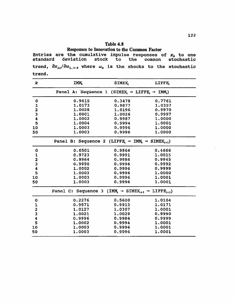
1 2 2

Table 4.8Responses to Innovation to the Common Factor

Entries are the cumulative impulse responses of xk to one standard deviation stock to the common stochastictrend, dxit/d(al t_k where o>lt is the shocks to the stochastictrend.k IMM, SIMEX, LIFFE,

Panel A: Sequence 1 (SIMEX, -* LIFFE, -* IMM,)0 0.9615 0.3478 0.77611 1.0173 0.9877 1.03572 1.0028 1.0196 0.99703 1.0001 1.0026 0.99974 1.0002 0.9987 1.00005 1.0004 0.9994 1.000110 1.0003 0.9996 1.000050 1.0003 0.9996 1.0000

Panel B: Sequence 2 (LIFFE, - IMM, - SIMEX,+1)0 0.6501 0.9864 0.46661 0.9723 0.9991 1.00152 0.9964 0.9986 0.99453 0.9990 0.9996 0.99924 1.0002 0.9996 0.99995 1.0003 0.9996 1.000010 1.0003 0.9996 1.000150 1.0003 0.9996 1.0001

Panel C: Sequence 3 (IMM, -*• SIMEX,+1 -» LIFFE,+1)0 0.2276 0.5600 1.01041 0.9571 0.9913 1.01712 1.0127 1.0307 1.00013 1.0021 1.0029 0.99904 0.9996 0.9986 0.99995 1.0002 0.9994 1.000110 1.0003 0.9996 1.000150 1.0003 0.9996 1.0001

123horizon, the innovations in the common factor explain 99% of the fluctuations in AIMM, but only 33% and 80% in ASIMEX and ALIFFE, respectively.

The impulse responses of Xx to an innovation to the common stochastic trend are reported in Table 4.8. In response to a shock generated at day 0 (the same day) , all markets fully respond in day 1 (next day) . Specifically, at day 0, the Chicago market responds 96%, the Singapore market 35%, and the London market 78%. Note that the long-run multiplier of the permanent shock is unity, i.e.,

limA.,oo0xit/3a)1( t_k = 1 where i = 1, 2 or 3 . ^l)

These results may imply that the common factor is mainly derived from the Chicago market, and the Chicago market drives the information transmission mechanism among markets, assuming that the common factor impounds all the long-run information.

Nevertheless, the aforementioned nonsynchronous trading problem is found to carry over to this section. In fact, the results in Panel B and Panel C, which follow Sequences 2 and 3, respectively, in Figure lb, show that whichever is the last trading market in the 24-hour trading sequence is the "dominant" market driving the common factor. That is, when Singapore is the last trading market as in Sequence 2, the Singapore market responds 99% at day 0, but 65% and 47% for the Chicago and London markets, respectively. Similarly, when

124London is the last trading market as in Sequence 3, it responds 100% at day 0, but 23% and 56% for the Chicago and Singapore markets respectively. Corresponding results of forecast error variance decomposition presented in Table 4.7 are also obtained. That is, if the last trading market in the 24-hour trading sequence is Singapore or London, at the end of a 1-day or 50-day horizon, 99% of the its forecast error variance can be explained by «lt.

In sum, none of the three markets can be described as the main source of information flow. Instead, each trading market is extremely informationally efficient, on a daily basis, and embodies all the information that will affect the two other nontrading markets when they open several hours later. It is worth mentioning that these results are not inconsistent with the results obtained in Section 4.3. Section 4.3 merely indicates that information is revealed during the nontrading hours of the Singapore market; here the results demonstrate that the Singapore market, and the other two markets, incorporates all the information when there is information flow.

4.7 Volatility Transmission and Spillover

Engle, Ito, and Lin (1990) provide empirical evidence of volatility transmission in the spot currency (yen/dollar) markets. They formulate two possible hypotheses which they name "meteor showers" and "heat waves." The heat wave null

125hypothesis maintains that volatility has only country-specific autocorrelation, whereas the meteor shower hypothesis implies volatility spillovers from one market to the next. Their empirical findings support the meteor shower hypothesis.

This section examines whether news in the one market can predict volatility in the other markets several hours later. Suppose that there was a large interest rate increase in the Singapore market. If the shock creates the expectation of more increase, then speculation may take place in the London market or the Chicago market on the same day and not wait until the Singapore market of the next day. The mutual settlement arrangement between the IMM and SIMEX may reinforce this meteor shower phenomenon. Before the empirical results are examined, it is worth noting that when one of the Eurodollar futures market close physically, one of the other two markets is already open. From this perspective, investors may consider the three markets as one combined market with the SIMEX beingthe opening section, the LIFFE the middle section, and the IMMthe closing section. The combined market then closes for fivehours (from the IMM close to the SIMEX open) until the nexttrading day beginning with the SIMEX. Hence, volatility spillovers from the SIMEX to the LIFFE or IMM, e.g., may be regarded as the spillovers from the open trading hours to the rest of the trading hours. In addition, the GLOBEX electronic systems introduced in July 1992 allow investors to trade during the closing section, from the IMM close to the SIMEX

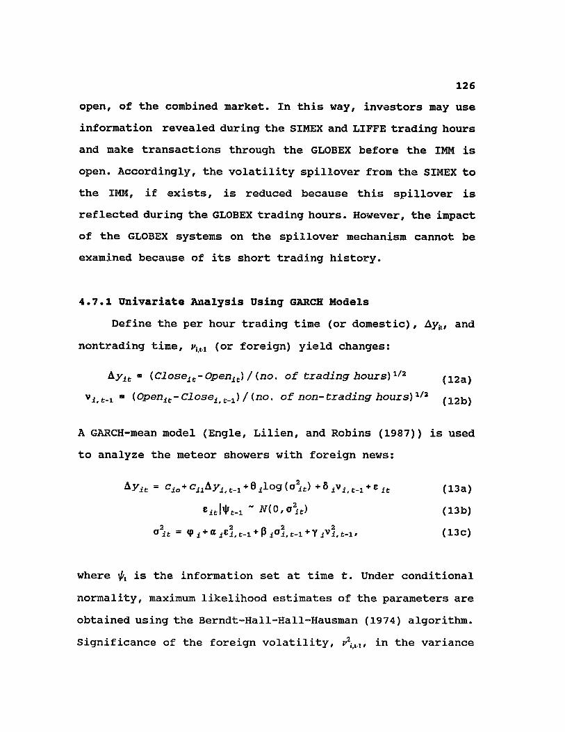
126open, of the combined market. In this way, investors may use information revealed during the SIMEX and LIFFE trading hours and make transactions through the GLOBEX before the IMM is open. Accordingly, the volatility spillover from the SIMEX to the IMM, if exists, is reduced because this spillover is reflected during the GLOBEX trading hours. However, the impact of the GLOBEX systems on the spillover mechanism cannot be examined because of its short trading history.

4.7.1 Univariate Analysis Using GARCH ModelsDefine the per hour trading time (or domestic), Aya, and

nontrading time, v (or foreign) yield changes:

Ayit - (Closeit - Openlt) / {no. of trading hours)1/2 (12a)vi, t-i " (Openit- Closel t_1) / (no. of non-trading hours)1/2 (i2b)

A GARCH-mean model (Engle, Lilien, and Robins (1987)) is used to analyze the meteor showers with foreign news:

where is the information set at time t . Under conditional normality, maximum likelihood estimates of the parameters are obtained using the Berndt-Hall-Hall-Hausman (1974) algorithm. Significance of the foreign volatility, v*itrl, in the variance

Ayit = cio + cilAyi/ t_x + 0 jlog (o\t) +6 j V ^ ^ + e it Eitkt-i ~ N ( 0 , o it)

a it = <P i+ a t-i+ P i°L t-i+ Y iVi, t-i * (13C)(13b)(13a)

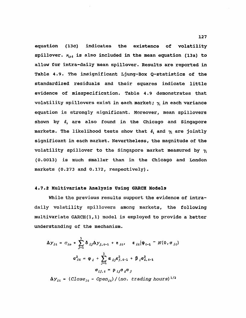
127equation (13c) indicates the existence of volatility spillover. pit., is also included in the mean equation (13a) to allow for intra-daily mean spillover. Results are reported in Table 4.9. The insignificant Ljung-Box Q-statistics of the standardized residuals and their squares indicate little evidence of misspecification. Table 4.9 demonstrates that volatility spillovers exist in each market; 7; in each variance equation is strongly significant. Moreover, mean spillovers shown by 5; are also found in the Chicago and Singapore markets. The likelihood tests show that and y-t are jointly significant in each market. Nevertheless, the magnitude of the volatility spillover to the Singapore market measured by yt (0.0013) is much smaller than in the Chicago and London markets (0.273 and 0.172, respectively).

4.7.2 Multivariate Analysis Using GARCH ModelsWhile the previous results support the evidence of intra

daily volatility spillovers among markets, the following multivariate GARCH(1,1) model is employed to provide a better understanding of the mechanism.

3by it = c±o + £ 5 ijbyjt t-i + eit, eit|i|rt-i ~ N(0,oit)

3

°ij. t ~ P ij° i° j Ayit = (Closeit - Openit) / (no. trading hours)1/2

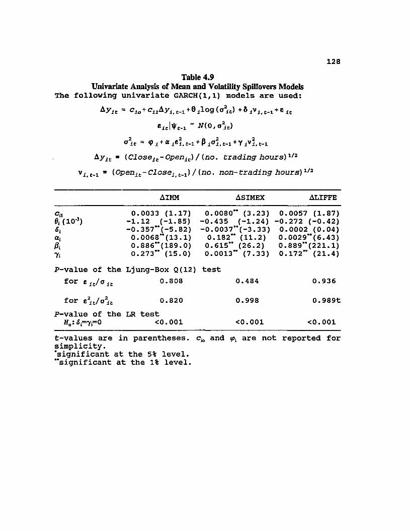
128Table 4.9

Univariate Analysis of Mean and Volatility Spillovers Models The fo llo w in g u n iv a r ia te GARCH(l,l) m odels a re u sed :

= <=io+ CuAyi.t-x + Q i lo g (o2Jt) +6 iV ^ ^ + e Jc

CitlVt-i ~ m o , o 2it)

o \ t = <P i + « iCi, t . i + P t . i + y iV i, t - i

Ayit ■ (Closeit-Openit) / (no. trading hours) 1/2

Vj f.! ■ (Openit-Closeiit_x) / (no. nontrading hours)1/2

AIMM ASIMEX ALIFFE

Cil 0.0033 (1.17) 0.0080** (3.23) 0.0057 (1.87)6i (i<r3) -1.12 (-1.85) -0.435 (-1.24) -0.272 (-0.42)Si -0. 357** (-5.82) -0. 0037**(-3 .33) 0.0002 (0.04)<*i 0. 0068*’ (13 .1) 0.182** (11.2) 0. 0029**(6. 43)A 0. 886** (189 . 0) 0.615** (26.2) 0. 889*’(221.1)7i 0.273*’ (15.0) 0.0013** (7.33) 0.172** (21.4)P-value of the Ljung-Box Q(12) test

f°r eit/oit 0.808 0.484 0.936

for e jt/o2it 0.820 0.998 0.989tP-value of the LR test

Ho:Srli=0 <0.001 <0.001 <0.001t-values are in parentheses, and ^ are not reported for simplicity.’significant at the 5% level.“significant at the 1% level.

129Note that t does not represent the calendar date, but the trading sequence. For example, in the IMM equation, yield changes of the SIMEX and LIFFE, which open earlier than the IMM, on the same calendar date are included. and are, ip^j, denote the coefficients of mean and volatility spillovers, respectively, from market j to market i. AIMM, ASIMEX, and ALIFFE are represented by i=l, 2, and 3, respectively. Under the assumption of time-invariant conditional correlations assumption (Bollerslev (1990)) , the cross products of the

standardized residuals, cite2t/ (°it02t) for should be

serially uncorrelated. Similar multi-GARCH models have been used by, e.g., Theodossiou and Lee (1993).

The results are reported in Table 4.10. Panel A shows that (i) for the IMM, there are mean spillovers from the LIFFE, and volatility spillovers from the SIMEX and LIFFE; (ii) for the SIMEX, there are mean and volatility spillovers from the IMM and LIFFE; and (iii) for the LIFFE, there are mean spillovers from the LIFFE, and volatility spillovers from the SIMEX. In short, in each market, mean and volatility spillovers exist at least from one other market. Panel C shows that the joint hypothesis of no mean and volatility spillover from market i to the other two markets are rejected at any conventional levels. These results reveal the interdependence among markets. In Panel B the Ljung-Box Q-statistics of the standardized residuals and their squares, and the cross

130Table 4.10

Multivariate Analysis of Mean and Volatility Spillovers Models The following Multivariate GARCH(1,1) models with constant conditional correlation are used:

3Ayit = cio + + eitl’i't-i ~ m o , a lt)

j=i3

°it = <Pi + £ a ijSi, t-1 + P t-1 > 1

Ayit = (Closeit - Openit) / (no. trading hours)1/2

and o , i^j, denote the coefficients of mean and volatility spillovers, respectively, from market j to market i. AIMM, ASIMEX, and ALIFFE are represented by i=l, 2, and 3, respectively.

Market i

AIMM ASIMEX ALIFFEA. Parameter Estimates

^i,AIMM -0.005* (-2.13) -0. 006** (-4 .57) 0.008” (2.64)i, ASIMEX 0.205 (1.44) 0.103” (4.29) -0.510**(-2 .16)^i,ALIFFE 0.718**(11. 51) 0.009” (4.91) -0.002 (-0.45)a i,AIMM 0.176**(10. 62) 0.002” (7.03) 0.002” (3.00)a i, ASIMEX 0.393** (3.71) 0.232” (9.77) 0.581” (8.04)a i, ALIFFE 0.169** (7.55) 0.002” (7.03) 0.004” (5.07)A 0.480** (15.73) 0. 382**(14.19) 0. 769**(73 .44)

Constant Conditional Correlation Coefficient pyAIMM 1.0 -0.125* (-2.01) 0.163* (2.33)ASIMEX 1.0 0.185* (2.18)ALIFFE 1.0

(table con'd.)

131

AIMM ASIMEX ALIFFEB. Diagnostic Tests

Ljung-Box test p-values of Q(12)for eit/oit 0.387 0.485 0.725

for e it/it 0.704 0.999 0.838

p-values of Q (12) for cross product of standardizedresiduals,

AIMMASIMEX

0.037* 0.1870.991

C. Joint Tests of Mean and Volatility Spillover*p-values of

the LR testHo:fia=os*0f <0.001 <0.001 <0.001

t-values are in parentheses. and <pK are not reported for simplicity."This tests the joint hypothesis of mean and volatility spillovers from market i to the other two markets, ’significant at the 5% level.’’significant at the 1% level.

1 3 2

product standardized residuals are found to be insignificant, except the cross product standardized residuals between AIMM and ASIMEX that is marginally significant with a p-value equal 0.037.

One distinct observation is that the volatility spillover from the SIMEX to the IMM and LIFFE is much stronger than that from the IMM or LIFFE to the SIMEX. Moreover, the volatility spillover from the SIMEX to the IMM and LIFFE is even greater than their own volatility spillovers. Specifically, the domestic volatility spillover (or heat wave) coefficients, otn and a33, in the IMM and SIMEX, are, respectively, 0.173 and 0.004, while the foreign volatility spillovers (or meteor showers) from the SIMEX, a12 and a32, are greater than an and a33 with values equal 0.393 and 0.581, respectively. However, the foreign volatility spillovers from the IMM (ot21) and LIFFE (a^) to the SIMEX are both only 0.002. This finding is unexpected, (though consistent with that in the univariate analysis), since, as previously examined, economic news affecting Eurodollar futures markets seems to come from the nontrading hours of the Singapore market. One possible reason for this strong spillovers from the Singapore market is the previously- mentioned combined-market proposition, i.e., the open volatility spillovers to the rest of the trading hours. However, this reason may not be very conclusive to explain such as a strong volatility spillover mechanism because the trading volume of the IMM is 10 times that of the SIMEX.

133Nonetheless, the above results should be interpreted with

caution because of the overlapping trading hours between the SIMEX close and the LIFFE open, and the LIFFE close and the IMM open. To partially purge the potential bias incurred by the overlapping trading hours among markets, only the two nonoverlapping Chicago and Singapore markets are examined, i.e., the LIFFE market is not included. Table 4.11 illustrates that the previously mentioned distinct phenomena (reported in Table 4.10) that there are strong volatility spillovers from the SIMEX to the IMM remain. To be more specific, the parameter showing volatility spillovers from the SIMEX to IMM, ae12, is 0.912, while that from the IMM to SIMEX is only 0.001. In this bivariate GARCH model, the Q-statistics of the standardized residuals and their squares, and the cross product standardized residuals are all insignificant.

4.7.3 Cross-market Spillover: U.S. Stock MarketsIt is not surprising that stock markets and interest rate

markets are interdependent. In fact, the Eurodollar (spot and futures) rates dropped significantly on the date of the October 1987 stock market crash. Would the volatility originating from the U.S. stock markets affect the spillover mechanism among Eurodollar futures markets?

An important institutional factor is that the New York Stock Exchange (NYSE), the highest trading volume stock exchange in the U.S., closes at 3:00 pm (Chicago time), while

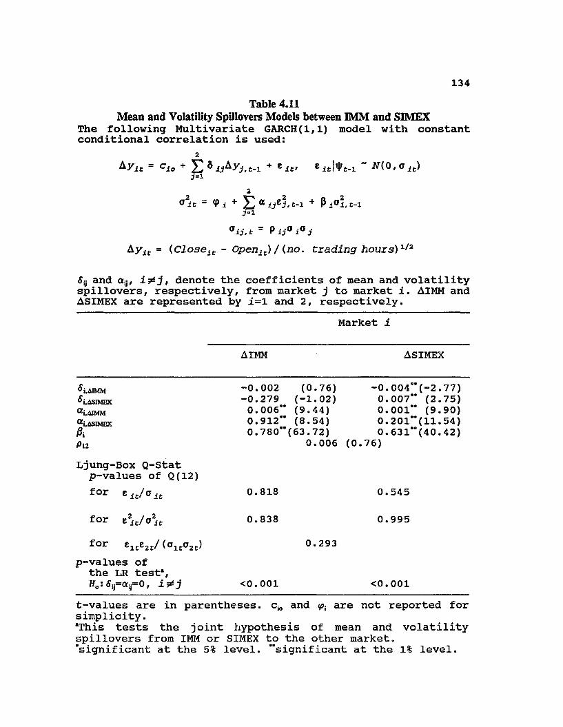
134Table 4.11

Mean and Volatility Spillovers Models between IMM and SIMEX The following Multivariate GARCH(1,1) model with constant conditional correlation is used:

2= cio + 6 iAYj. t-i + *it> e “ N(0,alt)

2°ifc = <Pi + + P jOi.t-i

aij.t =Ayit = (Closeit - Openit) / (no. trading hours)1/2

and ay, i&j, denote the coefficients of mean and volatility spillovers, respectively, from market j to market i. AIMM and ASIMEX are represented by i=l and 2, respectively.

Market i

AIMM ASIMEX

ft, AIMM ft, ASIMEX a i,AIMM a i,ASIMEXftPl2

-0.002 (0.76) -0.279 (-1.02) 0.006** (9.44) 0.912** (8.54)0.780** (63.72)

0.006

-0.004**0.007**0.001**0.201**0.631**

(0.76)

(-2.77)(2.75)(9.90)

(11.54)(40.42)

Ljung-Box Q-Stat p-values of Q(12)for 0.818 0.545

for *2 / _2 e it/°it 0.838 0.995for £ lte 2tf (°lt0 2t) 0.293

p-values of the LR test*, Ho:6~a~0, i*j <0.001 <0.001

t-values are in parentheses, c^ and <pt are not reported for simplicity.*This tests the joint hypothesis of mean and volatility spillovers from IMM or SIMEX to the other market, ’significant at the 5% level, “significant at the 1% level.

135the IMM closes at 2:00 pm. That is the IMM closes one hour earlier than the NYSE. Consequently, information revealed in the last trading hour of the NYSE cannot not be reflected in the IMM on the same date. Instead, this information is impounded into the SIMEX first, which opens earlier than the IMM and LIFFE on a calendar date basis.

Furthermore, both previous theoretical models (e.g., Admati and Pfleiderer (1988)) and empirical studies (e.g., Wood, Mclnish, and Ord (1985)) show that the NYSE is more volatile during its last trading hours than other trading hours. The source of the strong Singapore volatility to other markets documented in the previous two subsections may simply derive from the NYSE. This argument is supported by eliciting an example of high volatility happening in the NYSE during the period examined.

".... the Dow Jones Industrial Average plunges190.58 points [on 10/13/89]— most of it in thefinal h o u r " (The Wall Street Journal 10/16/89p.Cl).

The open and closing prices of the three ED markets for the two-trading-day window, 10/13/89 (Friday) - 10/16/89(Monday), is presented in Table 4.12. It shows that the closing price of the IMM, as well as the SIMEX and LIFFE, did not reflect the stock market drop since it had been closed on

136Table 4.12

An Example Showing the Cross-Market Volatility from the NYSE On 10/13/1989, the DJIA dropped 190 points. This occurred mainly during the last trading hour of NYSE. The IMM had been closed at that time, and the SIMEX is the first next open Eurodollar futures market.

IMM SIMEX LIFFEOpen Close Open Close Open Close

10/13/89 (Friday) 8.40 8.42 8.45 8.43 8.43 8.5310/16/89 (Monday) 7.96 8.32 7.80 8.04 7.92 8.2010/13 C - 10/13 O 0.02 -0.02 0.1110/16 O - 10/13 C -0.46 -0.63 -0.61

137that date. More specifically, the third row of the table indicate that the open-to-close yield changes on 10/13/89 are only 0.02, -0.02, and 0.11 at the IMM, SIMEX, and LIFFE.However, as shown in the fourth row, the open price on 10/16/89, dropped substantially from the last closing price; the differences are -0.46, -0.63, and -0.61, respectively for the three markets. This example reveals that if the U.S. stock markets, which might be the source of volatilities among Eurodollar futures, are not incorporated into the spillover mechanism, the Singapore market may be mis-interpreted to strongly volatility-spillover the IMM and LIFFE. This crossmarket transmission mechanism between Eurodollar futures and U.S. stock markets is being currently studied.

4.8 Conclusions

This chapter investigates the international transmission of information in Eurodollar futures markets. It analyzes the volatility of interest rates changes in each market during trading and nontrading hours. It is found that, in contrast to the other two markets, the nontrading time variance of the Singapore market is higher than the trading time variance. An approach exploring the common factor in the cointegration system is employed to examine the variance decomposition and impulse response functions of interest rates. All markets respond to the shock generated from the common factor rapidly.

138Comparing the results with different orderings of trading

sequence, each trading market is evinced to impound all the information that will influence the two nontrading markets when they open later in the day. Each market in turn drives the common factor and information flow. In this way, none of the three markets can be considered the main source of information flow. Instead, each trading market is extremely informationally efficient.

The meteor shower and heat wave models of Engle, Ito, and Lin (1990) are employed to investigate the volatility spillover among the three futures markets. Strong evidence of intra-daily volatility spillover from each of markets to the other two is given. More importantly, the source of the strong volatility spillover from the Singapore market to Chicago and London markets may be derived from the NYSE.

In conclusion, the Eurodollar futures markets are informationally efficient on a daily basis, and certain market dynamics lead to a continuation of volatility. Incorporating the US stock markets into the system warrants a better understanding of the international transmission of information in Eurodollar futures markets.

CHAPTER 5

SUMMARY AND CONCLUSIONS

Chapters 2 and 3 examine the relationships between U.S. and Eurodollar interest rates by using daily futures data for the period of 3/1/1982 - 2/22/1994. Characteristics of the Treasury bill and Eurodollar futures markets (high liquidity, low transaction costs and institutional restrictions, same trading hours and exchange) offer a more reliable analysis of the transmission mechanism of domestic and external interest rates than the corresponding spot markets.

In Chapter 1, controversial evidence of cointegration is given by different cointegration tests, which are likely to be biased by the GARCH effects as indicated by the Monte Carlo results of the Appendix. The reported VAR and ECM do not give a better forecast than the naive model. Market efficiency is maintained on the basis of forecasting. This chapter also evinces long memory between the Treasury and Eurodollar futures after the crash, but the source of long memory explored is not explicitly determined. Therefore, in addition to other evidence examined in this chapter, particularly the simultaneous equations model and the causality tests, the hypothesis of contemporaneous movement is not rejected.

Chapter 3 examines the volatility spillover mechanism between Treasury bill and Eurodollar futures markets. Although

139

140some preliminary statistics seem to support the hypothesis that these two futures interest rates share the same volatility process, which follows a GARCH process, this hypothesis is rejected by the common volatility test of Engle and Kozicki (1993). A further examination indicates that during erratic periods, TB and ED respond differently (even moving in opposite directions) because the risk premium between them dominates economic fundamentals. A bivariate EGARCH model which allows for asymmetric volatility influence of the TED spread, as well as that of the domestic market, is used to model the volatility spillover between markets. The model shows that the lagged TED spread change is the driving force of the volatility process, a finding that is robust to the pre- and post-crash period examination. The reason is that, when the TED spread is highly volatile, the financial market is in a state of uncertainty, and, accordingly, the (conditional) variance of interest rates increases. In particular, a large lagged change of the spread implies an increase in risk premium of Treasury bills over Eurodollar deposits. These influences are greater when the change is positive than when it is negative, suggesting asymmetric volatility spillovers from the TED spread changes.

Chapter 4 investigates the international transmission of information in Eurodollar futures markets. It is found that, in contrast to the other two markets (Chicago and London) , the nontrading time variance of the Singapore market is higher

1 4 1

than the trading time variance. These results suggest that relevant information reveals more during the trading hours of the IMM and LIFFE markets than those of the SIMEX market. An approach exploring the common factor in the cointegration system is employed to examine the variance decomposition and impulse response of functions of interest rates. All markets respond to the shock generated from the common factor rapidly. Comparing the results with different orderings of trading sequence, each trading market is evinced to impound all the information that will influence the two nontrading markets when they open later in the day. Each market in turn drives the common factor and information flow. In this way, none of the three markets can be considered the main source of information flow. Instead, each trading market is extremely informationally efficient. Strong evidence of intra-daily volatility spillovers from each of the markets to the other two is given. More importantly, the source of the strong volatility spillover from the Singapore market to Chicago and London markets may be derived from the NYSE. Incorporating the U.S. stock markets into the system, therefore, warrants a better understanding of the international transmission of information in Eurodollar futures markets.

In conclusion, the U.S. and Eurodollar interest rates are informationa1ly efficient with the TED spread playing an important role in the volatility spillover mechanism. The informational efficiency hypothesis on a daily basis is also

142

maintained in three international Eurodollar futures markets, and certain market dynamics lead to a continuation of volatility among them.

REFERENCES

Admati, A.R., and P. Pfleidere, 1988, A theory of intraday patterns: Volume and price variability, Review ofFinancial Studies 1, 3-40.

Aka ike, H., 1974, A new look at the statistical modelidentification, IEEE Transactions on Automatic Control 19, 714-723.

Andrews, D., 1991, Heteroskedasticity and autocorrelationconsistent covariance matrix estimation, Econometrica 59, 817-858.

Aydogan, K., and G.G. Booth, 1988, Are there long cycles in common stock?, Southern Economic Review, 141-149.

Arshanapalli, B., and J. Doukas, 1992, International stock markets linkages: Evidence from the pre and post-October 1987 period, Journal of Banking and Finance 17, 193-208.

Baillie, R.T. and R. J. Myers, 1991, Bivariate GARCH estimation of the optimal commodity futures hedge, Journal of Applied Econometrics 6, 109-124.

---------- , and T. Bollerslev, 1989, Common stochastic trendsin a system of exchange rates, Journal of Finance 44, 167-181.

— ------- -f a n d ---------— 1993, Cointegration, fractionalcointegration, and exchange rate dynamics, Northwestern University Working Paper.

---------- ,-- --------- -, and H.O. E. Mikkelsen, 1993,Fractionally integrated generalized autoregressive conditional heteroskedasticity, Northwestern University Working Paper.

------- -— , C.F. Chung, and M.A. Tieslau, 1992, The longmemory and variability of inflation: A reappraisal of the Friedman hypothesis, Tibury University, Discussion Paper.

Barclay, M.J., R. Litzenberger, and J.B. Warner, 1990, Private information, trading volume and stock return variances, Review of Financial Studies 3, 233-253.

Berndt, E.K., B.H. Hall, R.E. Hall, and J.A. Hausman, 1974, Estimation and inference in nonlinear structural models, Annals of Economic and Social Measurement 3/4, 653-665.

1 4 3

144Black, F., 1976, Studies of stock price volatility changes,

Proceedings from the American Statistical Association, Business and Economic Statistics Section, 177-181.

Bollerslev, T., 1986, Generalized autoregressive conditional heteroskedasticity, Journal of Econometrics 31, 307-327.

-■— ------, 1987, A conditional heteroskedastic time seriesmodel for speculative prices and rates of return, Review of Econometrics and Statistics 31, 542-547.

---- 1990, Modelling the coherence in short-runnominal exchange rates: a multivariate generalized ARCH model, Review of Economics and Statistics, 498-505.

-------- -— , and H.O. E. Mikkelsen, 1993, Fractionallyintegrated generalized autoregressive conditional heteroskedasticity, Northwestern University Working Paper.

Booth, G.G., M. Chowdhury, and T. Martikainen, 1993, Theinternational transmission of information in stock index futures markets, Louisiana State University Working Paper.

---------- , and M. Chowdhury, 1991, Long-run dynamics of blackand official Exchange Rates, Journal of International Money and Finance 10, 392-405.

---------- , and — , 1992, Canadian foreign exchangepolicies: intervention, control, and cointegration,Weitwirtschaftliches Archiv 128, 21-33.

---------- , and ----------, 1993, The effect of ownershiprestrictions on stock price dynamics". Working paper, Baton Rouge: Louisiana State University.

Bradley, M.G., and S.A. Lumpkin, 1992, The Treasury yield curve as a cointegrated system, Journal of Financial and Quantitative Analysis 27, 449-464.

Campbell, J.Y., and L. Hentschel, 1992, No news is good news: An asymmetric model of changing volatility in stock returns, Journal of Financial Economics 31, 281-318.

*----- , and R.J. Shiller, 1987, Cointegration and tests ofpresent value models, Journal of Political Economy 95, 1062-1088.

----------, and ----- — — , 1988, Interpreting cointegratedmodels, Journal of Economic Dynamic and Control, 505-522.

145Chan, K., and Y.P. Chung, 1993, Intraday relationships among

index arbitrary, spot, and futures price volatility, and spot market volume, Journal of Banking and Finance 17, 663-687.

Cheung, Y.W., 1993a, Tests for fractional integration: A monte carlo investigation, Journal of Time Series Analysis.

---------- , 1993b, Long memory in foreign-exchange rates,Journal of Business & Economic Statistics 11, 93-101.

-— , and K.S. Lai, 1993a, A fractional cointegrationanalysis of purchasing power parity, Journal of Business & Economic Statistics 11, 103-112.

---------- 1 and --- ----— , 1993b, Finite sample sizes ofJohansen's likelihood ratio tests for cointegration, Oxford Bulletin of Economics and Statistics 55, 313-328.

Connolly, R.A., 1989, An examination of the robustness of the weekend effect, Journal of Financial and Quantitative Analysis 24, 133-170.

Dickey, D.A. and W.A. Fuller, 1979, Distribution of the estimators for autoregressive time series with a unit root, Journal of American Statistical Association 74, 427-31.

------— — ■ , and ---------- , 1981, Likelihood ratio statisticsfor autoregressive time series with a unit root, Econometrica 49, 1057-1072.

Diebold, F.X., 1988, Empirical modelling of exchange ratedynamics, Springer-Verlag, New York.

-----------, 1986, Modelling the persistence of conditionalvariances: A Comment, Econometric Reviews 5, 51-56.

---------- , J. Gardeazabal, and K. Yilmaz, 1994, Oncointegration and exchanges Rate dynamics, Journal of Finance, forthcoming.

---------- , and M. Nerlove, 1989, The dynamic of exchangerate volatility: A multivariate latent factor ARCH model, Journal of Applied Econometrics 4, 1-21.

--- — f and G.D. Rudebusch, 1989, Long memory andpersistence in aggregate output, Journal of Monetary Economics 24, 189-209.

146

---------- , and ---------- , 1991, On the power of Dickey-Fuller tests against fractional alternatives, Economics Letter 35, 155-160.

Dornbusch, R., D.V. Dantas, C. Pechman, R.R. Rocha, and D. Simoes, 1983, The black market for dollars in Brazil, Quarterly Journal of Economics 98, 25-40.

Edwards, F.R., and C.W. Ma, 1992, Futures & Options, McGraw- Hill.

Engle, R.F., 1982, Autoregressive conditionalheteroskedasticity with estimates of the variance of United Kingdom inflation, Econometrica 50, 987-1007.

— -------— , and T. Bollerslev, 1986, Modelling the persistenceof conditional variances, Econometric Reviews 5, 1-50.

------— , 1990, Discussion: Stock market volatility and thecrash of 987, Review of Financial Studies 3, 103-106.

.------ / an(j c.W.J. Granger, 1987, Cointegration and errorcorrection: Representation, estimation, and testing,Econometrica, 55, 251-276.

---------- , T. Ito, and W.L. Lin, 1990, Meteor showers or heatwaves? Heteroskedastic intra-daily volatility in the foreign exchange market, Econometrica 58, 525-542.

, and S. Kozicki, 1993, Testing for common features,Journal of Business & Economic Statistics 11, 369-380.

---------- , D.M. Lilien, and R.P. Robins, 1987, Estimatingtime varying risk premia in the term structure: The ARCH- M model, Econometrica 55, 391-407.

---------- , and V. Ng, 1993, Measuring and testing the impactof news on volatility, Journal of Finance 48, 1749-1778.

-------- -, and R. Susmel, 1993, Common volatility ininternational equity markets, Journal of Business & Economic Statistics 11, 167-176.

---------- , and B.S. Yoo, 1987, Forecasting and testing incointegrated system, Journal of Econometrics 35, 143-159.

Ermini, L., and D.F. Henry, 1991, Log income vs. linear income: An application of the encompassing principle, Working Paper, Department of Economics, University of Hawaii at Manoa.

147Eun, C.S., and S. Shim, 1989, International transmission of

stock market movements, Journal of Financial and Quantitative Analysis 24, 241-256.

Fama, E.F., 1965, The behavior of stock market prices, Journal of Business 38, 34-105.

French, K.R., and R. Roll, 1986, Stock return variances: The arrival of information and the reaction of traders, Journal of Financial Economics 17, 5-26.

Friedman, M., 1983, Lessons from the 1979-82 monetary policy experiment, Journal of Money, Credit, Banking, 339-343.

-------- — , G.W. Schwert, and R.F. Stambaugh, 1987, Expectedstock returns and volatility, Journal of Financial Economics 19, 3-29.

-----------, and D.E. Sichel, 1993, Cyclical patterns in thevariances of economic activity, Journal of Business and Economic Statistics 11, 113-119.

Fuller, W.A., 1976, Introduction to Statistical Time Series, Wiley, New York.

Fung, H.K., and S.C. Isberg, 1992, The international transmission of Eurodollar and US interest rates: Acointegration analysis, Journal of Banking and Finance 16, 757-769.

---.--- # arui w.K., Leung, 1993, The pricing relationship ofEurodollar futures and Eurodollar deposit rates, Journal of Futures Markets 13, 115-126.

Geweke, J., and S. Porter-Hudak, 1983, The estimation andapplication of long memory time series models, Journal of Time Series Analysis 4, 221-238.

Giddy, I.H., G. Dufey, and S. Min, 1979, Interest rates in the US and Eurodollar markets, Weitwirtschaftliches Archiv 115, 51-67.

Gonzalo, J., 1994, Comparison of five alternative methods of estimating long run equilibrium relationships, Journal of Econometrics 60, 203-234.

-----------, and J.Y. Pitarakis, 1994, Testing forcointegration: New multivariate tests and a modelselection approach, Boston University.

148Granger, C.W., 1969, Investigating causal relations by

economic models and cross-spectral methods, Econometrica 37, 424-438.

---------- , 1986, Developments in the study of cointegratedeconomic variables, Oxford Bulletin of Economics and Statistics 48, 213-228.

----- -----, 1988, Causality, cointegration and control,Journal of Economic Dynamics and Control 12, 551-559.

-----------, and A. Escribano, 1986, The long-run relationshipbetween prices from an efficient market: The case of gold and silver, Discussion paper, San Diego: University of California at San Diego.

--------- -, and R. Joyeus, 1980, An introduction to long-memory time series models and fractional differencing, Journal of Time series Analysis 1, 15-39.

---------- , and T.H. Lee, 1988, Investigation of production,sales and inventory relationships using multicointegration and nonsymmetric error correction models, Journal of Applied Econometrics 4, 5145-5159.

----- , and P. Newbold, 1986, Forecasting Economic TimeSeries, 2nd. edn., San Francisco: Academic Press., Y., Ronald W.

Hakkio, C.S., and M. Rush, 1991, Cointegration: How short is the long run?, Journal of International Money and Finance 10, 571-581.

Hamao, Y., R. Masulis, and V. Ng, 1990, Corrections in price change and volatility across international stock markets, Review of Financial Studies 3, 281-308.

Harvey, A., E. Ruiz, and E. Sentana, 1992, Unobservedcomponent time series models with ARCH disturbances, Journal of Econometrics 52, 1-311.

Hertzel, M.G., C.S. Kendall, and P.E. Kretzmer, 1990, Thevolatility of asset returns during trading and nontrading hours: Some evidence from the foreign exchange markets, Journal of International Money and Finance 9, 335-343.

Hendershott, P.H., 1967, The structure of internationalinterest rates: The U.S. Treasury bill rate and theEurodollar deposit rate, Journal of Finance 22, 455-465.

149Hill, J., and T. Schneeweis, 1990, International

trading/nontrading time effects on risk estimation in futures markets, Journal of Futures Markets 10, 407-423.

Hosking, J.R.M., 1981, Fractional differencing, Biometrika 68, 165-176.

Hultman, C.W., 1990, The Environment of International Banking, Prentice Hall, New Jersey.

Hylleberg, S., and G.E. Mizon, 1989, A note of the distribution of the least squares estimator of a random walk with drift, Economics Letters 29, 225-30.

Jeon, B., and G.M. von Furstenberg, 1990, Growing international co-movements in stock price indexes, Quarterly Review of Economics and Business 30, 15-30.

Johansen, S., 1988, Statistical analysis of cointegrationvectors, Journal of Economic Dynamics and Control 12, 231-254.

— ..--------, 1989, The power of the likelihood ratio test forcointegration, Institute of Mathematical Statistics, University of Copenhagen.

, 1991, Estimation and hypothesis testing ofcointegration vectors in Gaussian vector autoregressive models, Econometrica 59, 1551-1580.

Kaen, F.R., and G.A. Hachey, 1983, Eurocurrency and national money market interest rates: An empirical investigation of causality, Journal of Money, Credit and Banking 15, 327-338.

, B.P. Helms, and G.G. Booth, 1983, The integrationof Eurodollar and U.S. money market interest rates in the futures market, Weitwirtschaftliches Archiv 119, 601- 615.

Kim, K. and P. Schmidt, 1993, Unit root tests with conditional heteroskedasticity, Journal of Econometrics 59, 287-300.

King, R.G., C.I. Plosser, J.H. Stock, and M.W. Watson, 1991, Stochastic trends and economic fluctuations, American Economic Review 81, 819-840.

Koch, P.D., 1993, Reexamining intraday simultaneity in stock index futures markets, Journal of Banking and Finance 17, 1191-1205.

150Koh, A., and K.C. Tsui, 1992, An intermarket comparison of

Eurodollar futures price volatility, Review of Futures Markets, 519-531.

Kolb, R.W., 1991, Understanding Futures Markets, Miami, Kolb.Kremers, J.J.M., N.R. Ericsson, and J.J. Dolado, 1992, The

power of cointegration tests, Oxford Bulletin of Economics and Statistics 54, 325-348.

Kroner, K.F. and J. Sultan, 1993, Time-varying distributions and dynamic hedging with foreign currency futures, Journal of Financial and Quantitative Analysis 28, 535- 551.

Kwack, S.Y., 1971, The structure of international interestrates: An extension of Hendershott's tests, Journal of Finance 26, 897-900.

Lamoureux, C.G., and W .D . Lastrapes, 1990a, Heteroskedasticity in stock return data: Volume versus GARCH effects,Journal of Finance 45, 221-229.

f and ---------— , 1990b, Persistence in variance,structural change, and the GARCH model, Journal of Business & Economic Statistics 8, 225-234.

Laux, P.A., and A.J. Senchack, 1992, Bid-ask spreads in Financial Futures, Journal of Futures Markets 12, 621- 634.

Lehmann, B.N., Fads, martingales, and market efficiency, 1990, Quarterly Journal of Economics 150, 1-27.

Ljung, G.M., and G.E.P. Box, 1978, On a measure of lack of fit in time series models, Biometrika 67, 297-303.

Lo, A.W., 1991, Long-term memory in stock market prices,Econometrica 59, 1279-1313.

-------- — , and C. MacKinlay, 1988, Stock market prices do notfollow random walks: Evidence from a simple specification test, Review of Financial Studies 1, 41-66.

Ma, K.C., M. Jeffrey, and W.A. Mattew, 1992, Rolling over futures contracts: A note, Journal of Futures Markets 12, 205-217.

MacKinnon, J.G., 1991, Critical values for cointegrationtests, in R.F. Engle and C.W.J. Granger (eds.), Long Run Economics Relationships, Oxford University Press, 267-76.

151Malliaris, A.G., and J.L. Urrutia, 1992, The international

crash of October 1987: Causality tests, Journal ofFinancial and Quantitative Analysis 27, 353-364.

Mandelbrot, B., 1963, The variation of certain speculativeprices, Journal of Business 36, 394-419.

— ,------- -, 1972, A statistical methodology for non-periodiccycles: from the covariance to R/S analysis, Annals of Economic and Social Measurement 1, 259-290.

McLeod, A.I., and W.K. Li, 1983, Diagnostics checking ARMA time series models using squared residual autocorrelations, Journal of Time Series Analysis 4, 169- 176.

Najand, M., H. Rahman, and Y. Yung, 1992, Inter-currency transmission of volatility in the foreign exchange futures, Journal of Futures Markets 12, 609-620.

Nelson, D.B., 1990, ARCH Models as Diffusion Approximations, Journal of Econometrics 45, 7-38.

-------- -, 1991, Conditional heteroskedasticity in assetreturns: A new approach, Econometrica 59, 347-370.

Newey, W.K., and K.D. West, 1987, A simple positive semi-definite, heteroskedasticity and autocorrelation consistent covariance matrix, Econometrica 55, 703-708.

Ng, V.K., and S.C. Pirrong, 1994, Fundamentals and volatility: storage, spreads, and the dynamics of metals prices, Journal of Business 67, 203-230.

Osterwald-Lenum, M., 1992, A note with quantiles of theasymptotic distribution of the maximum likelihood cointegration rank test statistics, Oxford Bulletin of Economics and Statistics 54, 461-472.

Perron, P., 1988, Trends and random walks in macroeconomic time series, Journal of Economic Dynamics and Control 12, 297-332.

Phillips, P.C.B., 1987, Time series regression with a unit root, Econometrica 55, 277-301.

---------- , 1988, Regression theory for near-integratedtime series, Econometrica 56, 1021-1043.

---------- , and P. Perron, 1988, Testing for a unit root intime series regression, Biometrika 75, 335-346.

152--------- , and S. Ouliaris, 1990, Asymptotic Properties of

Residual Based Tests for Cointegration, Econometrica 58, 165-93.

Reimers, H.E., 1991, Comparisons of tests for multivariatecointegration, Deutsche Bunndesbank, Frankfurt.

Reinsel, G.C. and S.K. Ahn, 1988, Asymptotic properties of the likelihood ratio test for cointegration in the nonstationary vector AR model, Technical Report, Department of Statistics, University of Wisconsin, Madison.

---------, and S.K. Ahn, 1992, Vector autoregressive modelswith unit roots and reduced rank structure: Estimation, likelihood ratio test, and forecasting, Journal of Time Series Analysis 13, 353-375.

Ross, S., 1989, Information and volatility: The no-arbitrage martingale approach to timing and resolution irrelevancy, Journal of Finance 44, 1-17.

Said, S.E., and D.A. Dickey, 1984, Testing for unit roots in autoregressive-moving average models of unknown order, Biometrika 71, 599-607.

Sargan, J.D. and A. Bhargava, 1983, Testing residuals from least squares regression for being generated by the gaussian random walk, Econometrica 51, 153-74.

Schwarz, G., 1978, Estimating the dimension of a model,Annuals of Statistics 6, 461-464.

Schwert, G. W., 1987, Effects of model specification on tests for unit roots in macroeconomic data, Journal of Monetary Economics 20, 73-103.

Sentana, E., 1991, Quadratic ARCH models: A potential reinterpretation of ARCH models as second-order Taylor approximations, Working paper (London School of Economics and Political Science, London).

Shoesmith, G.L., 1992, Co-integration, error correction and improved medium-term regional VAR forecasting, Journal of Forecasting 11, 91-109.

Siegel, D.R., and D.F. Siegel, 1989, Futures Markets, The Dryden Press.

Sims, C., 1972, Money, income and causality, American Economic Review 62, 540-552.

153---------- , 1980, Macroeconomics and reality, Econometrica 48,

1-48.Slentz, J., 1987, The TED spread, Market Perspectives, Chicago

Mercantile Exchange 5, 1-4.Sowell, F.B., 1990, Fractional unit root distribution,

Econometrica 58, 495-505.Sowell, F.B., 1992a, Modelling long run behavior with the

fractional ARIMA, Journal of Monetary Economics 29, 277- 302.

---------- , 1992b, Maximum likelihood estimation of stationaryunivariate fractionally integrated time series models, Journal of Econometrics 53, 165-188.

Swanson, P.E., 1988, The international transmission ofinterest rates: A note on causal relationships between short-term external and domestic US dollar returns, Journal of Banking and Finance 12, 563-573.

Theodossiou, P., and U. Lee, 1993, Mean and volatility spillovers across major national stock markets: Further empirical evidence, Journal of Financial Research 16,337- 350.

White, H., 1980, A heteroskedasticity-consistent covariance matrix estimator and direct test for heteroskedasticity, Econometrica 48, 817-838.

Wood, R.A., T.H. Mclnish, and J.K. Ord, 1985, An investigation of transactions data for NYSE Stocks, Journal of Finance 40, 723-739.

Yajima, Y., 1988, On estimation of a regression model with long-memory stationary errors, The Annals of Statistics, 16, 791:807.

APPENDIX

COINTEGRATION AND FRACTIONAL COINTEGRATION TESTS WITH CONDITIONAL HETEROSKEDASTICITY:

A MONTE CARLO INVESTIGATION

A.1 Introduction

Despite the extensive literature on autoregressive conditional heteroskedasticity (ARCH) of Engle (1982), generalized ARCH (GARCH) of Bollerslev (1986), and related models, relatively little attention has been given to the issue of the GARCH effects on the performance of cointegration and fractional cointegration tests. This paper examines this issue by using a Monte Carlo approach.

A.l.l Cointegration TestsThe main assumption of the Johansen's (1988) likelihood

ratio tests for cointegration is that the disturbances in vector error correction models are i.i.d. Gaussian. A Monte Carlo experiment is conducted to analyze the empirical size and power of the Johansen test statistics in finite samples under the presence of conditional heteroskedasticity of the GARCH form. Comparisons are also conducted with the tests of Dickey and Fuller (1979, DF hereafter) and Sargan and Bhargava (1983) .

Kim and Schmidt (1993, KS hereafter) examine the DF unit root tests when the errors are conditionally heteroskedastic.

154

155When the unconditional variance does not exist (in the case of integrated GARCH) they find serious size distortion of the DF tests for some choices of the GARCH parameter values. When the unconditional variance of the first difference of an integrated series exists, the DF tests over-reject but only moderately. In this paper it is observed that the results of KS for the DF unit root tests with GARCH errors generally carry over to cointegration tests under the presence of GARCH errors.

Other Monte Carlo studies by Reimers (1991), Reinsel and Ahn (1988, 1992), and Cheung and Lai (1993b) have examined the effect of dynamic components of the system and non-Gaussian error distribution on the performance of the Johansen tests. Gonzalo and Pitarakis (1994) examine the effect of the dimension of the system on the size of the Johansen tests. It is found that the Johansen procedures tend to find cointegration more often than what asymptotic theory suggests. Several adjusted Johansen statistics have thus been proposed to improve the small sample performance. No adjustment is adopted here as the critical values are also simulated with the same seed to generate random numbers in all experiments in the paper.

Using the response surface analysis, Cheung and Lai (1993b) examine the bias in the test size due to non-normal innovations, including non-symmetric and leptokurtic ones. A commonly known source of leptokurtic innovations is

156conditional heteroskedasticity, which leads to a heavy-tailed distribution. Cheung and Lai find that both the Johansen maximum eigenvalue test and the Johansen trace test are reasonably robust to excess kurtosis although the trace test is found to be more robust. Their results are generally consistent with the results in this paper, in that the trace test has smaller size distortion under the presence of GARCH than the maximum eigenvalue test.

In this paper, results of Cheung and Lai (1993b) are examined more specifically by considering the case that the error variances follow a GARCH(1,1) model. The experiment conducted is an extension of the work on unit root tests by KS for the cointegration tests. It examines the empirical size and power of the Johansen trace test (trace, hereafter) and the Johansen maximum eigenvalue test (X^) . For comparison, it also considers the DF tests and the cointegrating regression Durbin-Waton test (CRDW) studied by Sargan and Bhargava (1983). The DF r-statistic (denoted t ) is the usual t-value from the DF OLS regression, and another DF test statistic, T(p-l), is obtained using the OLS estimate of the first order autoregressive coefficient p of the DF regression and the sample size T.

Following KS, the DF T-statistic with White's (1980) correction for heteroskedasticity is also examined. In computing the size and power of the r statistic with the White correction, two different critical values are used. The

157critical value is obtained from the 5% low tail percentile of the DF t-statistic with the White correction; the other critical value is obtained from the 5% low tail percentile of the DF r-statistic without the correction (the same one used to report the results for t ) . The size and power using the first critical value (with the White correction) are reported under the notation "t-White", and the results using the second critical value are reported under the notation "r'-White".

The current results are similar and confirm the results of Cheung and Lai (1993b) and KS. These cointegration tests tend to over-reject the null hypothesis of no cointegration in favor of finding cointegration too often in the presence of GARCH errors, but the bias is not very serious except when the variance processes are nearly degenerate and integrated. The results of KS for the DF unit root tests with GARCH errors are generally observed for cointegration tests with GARCH errors. The trace test is often found to have smaller size distortion than the maximum eigenvalue test.

A . 1.2 Fractional Cointegration TestsIn the second part of the paper, similar Monte Carlo

experiments will be performed for fractional cointegration. Two widely used tests for fractional integration— Geweke and Porter-Hudak (GPH) (1983), and the modified rescaled range (MRR) of Lo (1991)— are examined.

158In the classical paradigm for cointegration, and indeed

in the Johansen procedure, all the elements of the Yt vector are assumed to be 1(d) processes with d=l (or an integer), while the cointegrating linear relationship a'Yt is presumed to be I (d-b) with Jb=l. This is referred to as Cl (1,1) . The Granger Representation Theorem, however, only requires that the cointegrating vector z,=a'Yt be stationary. Specifically, the strict 1(1) and 1(0) distinction is arbitrary. That is for the equilibrium error to be mean-reverting, it does not have to be 1(0) exactly. Fractionally integrated processes, as discussed by Granger and Joyeux (1980) and Hosking (1981), also display mean reversion. In this case the error correction term responds more slowly to shocks so that deviations from equilibrium are more persistent. The error correction term is depicted to process long memory.

The Autoregressive Fractionally-Integrated Moving Average (ARFIMA) representation is a natural extension of ARIMA models:

<j>(L) (1-L) dYt = 0(L)ec (1)

where d can take on non-integer values. A wide range of low frequency behavior can thus be modeled when d is not restricted to the integer domain. For the process to be covariance stationarity d<0.5, while invertibility requires that d>-0.5. One can always transform a fractionallyintegrated series of higher order (d>0.5) into the range of

159(-0.5, 0.5) by taking a suitable number of integer differences. Also, the cumulative impulse response coefficientscorresponding to a shock in the infinite past equal zero for d<l. The ARFIMA model displays long memory, that issubstantial dependence between observations k periods apart, even for large k.1 A long-memory model incorporatingconditional heteroskedasticity is rarely constructed. For example, Diebold and Rudebusch (1989) and Cheung (1993b), respectively, examine long memory in U.S. aggregate output and foreign rates by estimating ARFIMA. But the ARCH effect is not incorporated in their estimation methods. An exception is Baillie, Chung, and Tieslau (1992), who extend the ARFIMA process with the GARCH process to consider the effect of innovations on inflation and re-examine the Friedman hypothesis concerning the relationship between the mean and variance of inflation. They estimate the ARFIMA(0,d ,1)- GARCH(1,1) models for the inflation rates of U.S. and nine other countries. Accordingly, the performance of the tests for fractional integration, particularly in small samples, in the presence of ARCH effects should be examined in more details.

In a univariate analysis, Cheung (1993a) using Monte Carlo method shows that the GPH test and the MRR test are robust to moderate ARCH effects. However, he merely investigates the size test of the simplest ARCH model—

‘For large lags, the ARFIMA autocorrelations decline at a very slow hyperbolic rate. In contrast, ARMA autocorrelations decline in a rapid geometric rate.

160ARCH(1), which restricts the persistence in the variance last only one period. The ARCH parameter in the conditional equation is set equal to 0.1, 0.3, 0.5, 0.7 and 0.9; theconstant term <p0 is set equal to 1. He reports that "the only significant deviation from the nominal 5% size is the case of 01=O.l." (p.335) (For T=100, the MRR and GPH tests are 8% and 6.7%, respectively.) Cheung (1993a) provides no explanation for these unexpected results showing that the smallest ARCH parameter gives the poorest size performance. One possible reason is that <p0 is held constant in his experiment, instead of the unconditional variance, <pj (1-^) .2 The latter approach is adopted in KS and Engle and Ng (1993, p.1760). Cheung also investigate the Langrange multiplier (LM) type test for fractional integration. Since this method is not widely used in the literature, it is not examined in this Appendix.

A.2 The Simulation Design

A.2.1 Cointegration TestsIn the experiment for examining the size of the test,

bivariate and trivariate non-conintegrated systems with GARCH(1,1) error are generated as follows. Let Xt = (xlt... x ni) 't t = !»•••/ T+50, be an Nxl vector of integrated series with AXj = £,. The error vector ^ = (elt— eNt) 1 is assumed to

2Moreover, the simulation results are based on 1000 replications only.

161follow an N-variate conditional normal distribution with

E =0 and E l e j -a2Jt, (2)

where i = 1, ... , W, is the a-field generated by allinformation available at time t-1, and

o2it = 4> io + 4> ii e|, t-i+ <l> , t-i • (3)

Let uk = ek lok , be i.i.d. with E[uk]=0, var(uk), and E ^ u ^ O ,

Drawings of the pseudo random innovations uk, for i = 1, ..., N, and t = 1, ... , T+50, are performed from the standard normal distribution using SHAZAM 6.2 at the IBM TSO operating system. The first 50 observations are discarded.

Consider T = 100, 1000 and N = 2 , 3 with various choices of parameter values of (0iO, 0a, 0B), i = 1, ..., N. As theparameter values (0 , 0a, 0^) for all i (except for Table A.7) are the same, the simpler notation at2 and (0O, <pu 02), omitting the index i in reporting the results are used. T=1000 is used to examine the large sample properties for the case when the asymptotic theory is not available.

All simulations are based on 10,000 replications. The reported results are at the nominal 5% significance level. Note that the 95% confidence interval of the empirical size is

162(0.0456, 0.0544).3 In all simulations to compute the residual- based test statistics, such as r, T(p-l), and CRDW, xlt is used as the dependent variable in the cointegrating regressions (except for Case B in Table A. 7 where xm is used as the dependent variable).

In the experiment for examining the power of the tests, bivariate cointegrated series with GARCH errors are generated. Trivariate models (W=3) are not reported to save space. The system generated is:

A.xlt = -0 .2 (x1( -x2i t_j_) +®it an£i &X2t = e2t* (4)

where elt and have the conditional variances of theGARCH(1,1) form discussed above. As only a particular data generating process (DGP) is considered, the results simply be illustrative. For a general study, see the method used in Johansen (1989) who investigates the power function using the theory of near-integrated processes developed in Phillips (1988) .

For consistency, in computing the size and power of each test the simulated critical values reported in Table A.A.l are used. The critical values for T = 100, 1000 and N = 2, 3, are generated based on 10,000 replications. Moreover, in order to work with same random numbers, the same seed for all the

3Since if the true nominal size is s (s=0.05 for this paper), the observed size follows the asymptotic normal distribution with mean s and variance s(l-s)/10000 for 10,000 replications.

163simulations are utilized. The Monte Carlo study is organized as follows. Tables A.1.1, A.1.2, A.3, A.4, A.5, A.6, and A.7 show the empirical size of tests, the frequency that the null hypothesis stating that truly non-cointegrated processes are not cointegrated is rejected in 10,000 trials. Table A.2 shows the empirical power of tests, the frequency that the null hypothesis stating that truly cointegrated processes are not cointegrated is rejected in 10,000 trials. {uk} are generated from the standard normal distribution, except for Table A.5 where {Uj,} are drawn from the Student-t distribution. Asymmetric conditional heteroskedasticity of the exponential GARCH (EGARCH) form and the time-varying conditional covariance are also considered in Table A.6, respectively. Finally Table A.7 considers different GARCH parameter values for each variable in the system.

A.2.2 Fractional cointegration TestsGPH (1983) propose a semi-nonparametric procedure to test

for fractional integration. The procedure is motivated by the log spectral density of the ARFIMA process, and amounts to estimating the least squares regression

ln{J(Oj)} = P0+piln{4sin2(a)j/2)} +v\jt j=l,...,K

with /J,=-d, where J( •) is the periodogram of {Y,} at frequencyWj, Wj=2rrj/T (j=l, T-l) . There is evidence of fractionintegration if b, is significantly different from zero.

164Furthermore, the variance of the estimate of bt is given by the usual OLS estimator, and the theoretical asymptotic variance of the regression error i\ is known to be equal to it2/6, which can be imposed to increase efficiency. With a proper choice of the sample size for the GHP regression (5), n, the asymptotic distribution of bt depends on neither the order of the AJRMA part nor the distribution of the error term. It is suggested to set n=T’ with v= 0.5. For statistical completeness, j>=0.40, 0.45, 0.55, 0.60, 0.65, and 0.70 arealso examined. The virtue of this frequency domain regression method is that it permits estimation of d without knowledge of p and g in ARFIMA(p, d,q) . Note that the maximum likelihood estimation in the time domain by Sowell (1992a,b) is not considered because it is computationally very difficult, though it is more efficient.

Mandelbrot (1972) has shown that the R/S statistic is a more general test of long-term dependency in time series than either autocorrelation tests or examination of spectral densities. He points that, in particular, it is robust to changes in periodicity. However, Aydogen and Booth (1988) point out that conclusions drawn from the R/S statistic must be conditioned on the validity of its underlying assumptions, e.g., serial independence, which are routinely violated. Particularly, Lo (1991) argues out that one limitation of the R/S statistic is that it cannot distinguish between short- and long-term dependency, nor is it robust to heteroskedasticity.

165Lo modified the R/S statistic so that it is more robust to violations in the assumption that returns are i.i.d. The modification consists of replacing the standard deviation with an estimate that explicitly models short-term temporal dependency using the autocovariances up to a finite number of lags, weighted by factors proposed by Newey and West (1987):

MRR = — k = [ m a x ^ r E " minlstsT£ (Yt-Y)],JTV £ 1 £ 1

where

a2* = a2 + 2 ^ 2 ( y ± - y ) ( y ^ - y ) (?)

T (Yt-Y)2 (8)o2 - Ec-iq = Jnt{(3r/2)1/3[2p/(l-p)]2/3} (9)

where q is the number of lags in the weighted autocovariance function used to adjust MRR, and is set by Andrews (1991). q=0, 1, 5, 10 and 25 are also analyzed. The case of g=0corresponds to the traditional R/S statistic.

The random number generating procedure is similar to that of cointegration tests in previous subsection.

The error correction term, zt, is obtained from the OLS,

(10)

It follows from Yajima (1988) and Cheung and Lai (1993a) that if all elements of Yt are 1(1) and they are fractionally

166cointegrated, the OLS estimator of a is consistent and converges at the rate of TM . The GPH and MRR tests are then applied to the error correction term. From a practical point of view, as pointed out by Diebold and Rudebusch (1989), it makes no difference whether u, is estimated in levels or first difference, though the latter is more common.

As pointed out by Cheung and Lai (1993a), in testing for fractional cointegration, the critical values for the GPH and MRR tests derived from the standard distribution cannot be used directly to evaluate the GPH estimate of d. The reason is that et is estimated from the OLS regression which minimizes the residual variance of the cointegrating regression; accordingly, the residual series thus obtained tends to bias toward being stationary. The null hypothesis of no cointegration will then be rejected too often.4 Therefore, the empirical size of the GPH and MRR tests are obtained by simulation. The Monte Carlo experiment is conducted by RATS 4.2 at 486 PC, and the critical values of the GPH test and the MRR statistic are reported in Table A.A.2.

A.3 Results of the Simulation

A.3.1 Cointegration TestsTable A. 1.1 contains the results on the size of the tests

for N=2 and Table A. 1.2 for N= 3. The condition for the

4A analogous problem in testing for cointegration using unit-roots is discussed by Engle and Granger (1987).

167

Table A.1.1The Size of the Tests at 5% LevelN = 2; 0O = o0\l-4>r^ , <r„2 = 1

T 100 1000 100 1000 100 1000 100 1000

Panel A

(01 >02) (0.3,0.6) (0.3,0.65) (0.3,0.699) (0.3,0.7)

> W (r=0) 0.0698 0.0615 0.0749 0.0697 0.1431 0.1469 0.3906 0.9579trace (r=0) 0.0658 0.0612 0.0731 0.0697 0.1322 0.1346 0.3718 0.9537C R D W 0.0724 0.0642 0.0787 0.0805 0.0980 0.2027 0.2383 0.9221Tip-1) 0.0716 0.0605 0.0769 0.0779 0.1147 0.2729 0.3047 0.9632r 0.0714 0.0609 0.0774 0.0773 0.1154 0.2730 0.3158 0.9662r-White 0.0471 0.0396 0.0453 0.0385 0.0522 0.0301 0.0805 0.0763r'-White 0.0897 0.0654 0.0867 0.0626 0.0971 0.0520 0.1326 0.1009

Panel B

(01 >02) (0.1,0.8) (0.1,0.85) (0.1,0.899) (0.1,0.9)

K* (r=0) 0.0546 0.0503 0.0583 0.0538 0.0779 0.0930 0.0841 0.3718trace (r— 0) 0.0535 0.0510 0.0564 0.0533 0.0748 0.0833 0.0798 0.3418C R D W 0.0547 0.0510 0.0558 0.0541 0.0602 0.1022 0.0618 0.32987 T M ) 0.0561 0.0478 0.0566 0.0504 0.0644 0.1211 0.0678 0.4299r 0.0549 0.0484 0.0564 0.0524 0.0655 0.1219 0.0705 0.4436r-White 0.0504 0.0434 0.0497 0.0436 0.0543 0.0377 0.0570 0.0366r'-White 0.0999 0.0739 0.1004 0.0725 0.1098 0.0652 0.1128 0.0595

168

Table A.1.2The Size of the Tests at 5% LevelN = 3; (f>0 = <r„2 = 1

T 100 1000 100 1000 100 1000 100 1000

Panel A

(0.3,0.6) (0.3,0.65) (0.3,0.699) (0.3,0.7)

K* (r=0) 0.0757 0.0687 0.0846 0.0887 0.1842 0.2351 0.5883 0.9990trace (r=0) 0.0738 0.0627 0.0837 0.0795 0.1827 0.2820 0.6005 0.9995C R D W 0.0679 0.0679 0.0713 0.0815 0.0863 0.2022 0.2430 0.9597T(p-1) 0.0691 0.0695 0.0741 0.0841 0.1016 0.2721 0.3115 0.9758T 0.0713 0.0717 0.0764 0.0848 0.1053 0.2747 0.3286 0.9772r-White 0.0437 0.0406 0.0420 0.0361 0.0465 0.0247 0.0704 0.0691r'-White 0.0878 0.0594 0.0834 0.0546 0.0857 0.0382 0.1148 0.0887

Panel B

( 1)4*2) (0.1,0.8) (0.1,0.85) (0.1,0.899) (0.1,0.9)

Xnu, (r = 0) 0.0530 0.0531 0.0559 0.0583 0.0821 0.1199 0.0917 0.5855trace (r=0) 0.0572 0.0532 0.0587 0.0558 0.0824 0.1103 0.0952 0.5991C R D W 0.0553 0.0547 0.0544 0.0579 0.0553 0.0987 0.0580 0.37983TP-D 0.0544 0.0526 0.0550 0.0570 0.0607 0.1225 0.0640 0.4652r 0.0561 0.0548 0.0566 0.0576 0.0630 0.1247 0.0661 0.4792r-White 0.0485 0.0464 0.0480 0.0477 0.0560 0.0348 0.0569 0.0309r'-White 0.0990 0.0724 0.0980 0.0707 0.1024 0.0546 0.1041 0.0444

169existence of the unconditional fourth moment is 3<p2 +2<f>t<p2+<f>2 < 1 (Bollerslev, 1986); accordingly, the condition is 02<O.6O6 if 0!=O. 3, and 02<O.89O if 0t=O. 1. But this condition does not affects the results reported. Nevertheless, when the unconditional second moment does not exist or when 01+02=1, especially when 0t is large, the size distortion is very serious. In many applications with high frequency financial data the estimate for 0j+02 turns out to be very close to one and 0O is almost zero. For example, French, Schwert, and Stambaugh (1987) obtain the sum of the GARCH parameters equal to 0.996 and a very small (but significant) estimate 0o=6xlO‘7 for a daily stock market return process. For the same value of the sum 0t+02, the size distortion is bigger with a higher (see also Table A.4) . The size bias increases with sample size T for 0!+02 = 0.999 and 1, while it decreases with T for 0t+02 = 0.9 and 0.95. The problem is more serious for the larger system with N=3 than for the system with N=2, which is consistent with Gonzalo and Pitarakis (1994).

As KS conclude that the White correction for r for testing unit root is generally helpful, this paper also considers it for testing cointegration. The results in Table A.1 shows that the White's correction substantially improves the size distortion problem.

However, even if this optimistic perspective is taken for r-White or r '-White statistic, the story is only half-told, since the power of the tests must come into question. Table

170A.2 presents the results of the power tests. Although KS (p. 293) notice that the empirical size falls significantly below the nominal size, especially for large T, they did not examine the power performance. According to the system generated in (3) (for N= 2 ) , the error correction term w^x^x* follows an AR(1) model with the first autoregressive coefficient equals to 0.8, i.e., wt = 0.8wn + ft, where ft=eu-e2, is a white noise. A comparable simulation result when (<pu <p2) = (0,0) and T = 100 may be found in Engle and Granger (1987, Table II), where the power of CRDW and r tests are related for the case when wt = 0.8wt_, + ft although their DGP is not the same as (3). The power of the Johansen tests in Table A.2 for T = 100 is quite impressive and much higher than that of the DF and CRDW tests.

Another interesting aspect of the results in Table A. 2 is the poor empirical power of t-White and t '-White statistics. The power of t-White is lower for T=100 relative to the other tests. As the sample size increases so does the power of all tests, but even at T=1000, the power of t-White and t '-White is very low for (0!,02) = (0.3,0.7) . This suggests that the White correction for heteroskedasticity may not be the proper way for testing cointegration. For simplicity, results for t- White and r '-White are not reported hereafter.

Table A. 1 shows that the tests perform poorly when the GARCH processes are integrated (01+^2=1) and degenerate (0o=O). Thus we ask whether integratedness or degeneracy causes the problem. To examine this, 0t+02 is fixed at 1 and <pQ is varying

1 7 1

Table A.2The Power of the Tests at 5% LevelN = 2; <f>0 = <r02 = 1

T 100 1000 100 1000 100 1000 100 1000

Panel A

( (0.0,0.0) (0.3,0.6) (0.3,0.65) (0.3,0.7)

(r=0) 0.9878 1.0000 0.9614 1.0000 0.9504 0.9999 0.9195 1.0000trace (r=0) 0.9832 1.0000 0.9561 1.0000 0.9446 0.9999 0.9097 1.0000C R D W 0.6951 1.0000 0.6863 1.0000 0.6791 1.0000 0.6128 1.0000T(P-1) 0.6671 1.0000 0.6603 1.0000 0.6554 0.9999 0.6736 1.0000r 0.6667 1.0000 0.6630 0.9999 0.6561 0.9999 0.6891 1.0000r-White 0.5282 1.0000 0.3495 0.9922 0.3257 0.9741 0.1907 0.2658r'-White 0.7271 1.0000 0.5193 0.9936 0.4894 0.9807 0.3033 0.3383

Panel B

(4>i >$2) (0.1,0.8) (0.1,0.85) (0.1,0.9)

> W (r=0) 0.9743 1.0000 0.9677 1.0000 0.9261 1.0000trace (r=0) 0.9791 1.0000 0.9743 1.0000 0.9340 1.0000C R D W 0.6955 1.0000 0.6923 1.0000 0.6681 1.0000TXp-l) 0.6651 1.0000 0.6619 1.0000 0.6550 1.0000T 0.6665 1.0000 0.6667 1.0000 0.6573 1.0000r-White 0.4679 1.0000 0.4597 1.0000 0.4432 0.9844r'-White 0.6634 1.0000 0.6534 1.0000 0.6309 0.9919

A x u = -0.2(x,n - x2iu) + elt and Ax2l = e*.

172in Panel A Table A.3, following KS's Table 2; while in Panel B, 0O is fixed at 0.01 and <Pi+<p2 is varying. It is found that the results are very similar to those of the DF unit root tests in KS. That is, degeneracy rather than integrated GARCH appears to drive the serious over-rejection problem. For example, in Panel A, when 0O decreases from 0.01 to 0.0 for T=100, the empirical size of the trace increases from 0.0915 to 0.3906; in Panel B, when 0j+02 increases from 0.95 to 1.0, the size only rises from 0.0826 to 0.0915.

To be comparable with KS's results (Table 4 and 5) , Table A.4 reports the results that follows the parameterization of Nelson (1990), where 0O = 0.01y,ipl = 0.3ym , <j>2 = 1 and cr02 = 1. As 7 declines the GARCH process becomes degenerate. The results are similar to those of KS. The performance of the tests now improves as y declines although it approaches to degeneracy. It indicates that the high values of 0t may also cause the problem. This is also observed in Table A.l, where the size distortion is more serious when 0, = 0.3 than when 0t = 0.1. The size distortion is aggravated as T increases.

So far {uH} is generated from the standard normal distribution. Table A.5 illustrates the results of the series {uj simulated from the Student-t distribution with the degrees of freedom (v) being equal to 4 and 8. The kurtosis of the Student-t density is given by 3 (v-2) / (v-4) for v>4; and hence, it is 4.5 for v=8. The values of v are chosen based on the empirically estimated v by Bollerslev (1987), Baillie and

1 7 3

Table A.3The Size of the Tests at 5% Level

N = 2

Panel A: <t>x — 0.3, <t>2 = p II 1

4>o 0 0.01 1 100

T 100 1000 100 1000 100 1000 100 1000

(r=0) trace (r=0) C R D W Tip-1)T

0.39060.37180.23830.30470.3158

0.95790.95370.92210.96320.9662

0.09150.08850.08780.09080.0901

0.11480.10830.13130.13250.1321

0.08290.08010.08480.08420.0830

0.12860.12200.11750.10490.1059

0.0839 0.1290 0.0805 0.1229 0.0848 0.1175 0.0841 0.1043 0.0827 0.1058

' Panel B: </>c, = 0.01, cr02 = 1

(01)^2) (0.3,0.6) (0.3,0.65) (0.3,0.7)

T 100 1000 100 1000 100 1000

> W (r=0) trace (r=0) C R D W 7T(p-l)T

0.0712 0.0601 0.0693 0.0549 0.0727 0.0812 0.0717 0.0987 0.0715 0.0989

0.08260.07870.07960.07850.0794

0.06900.06580.09300.11010.1086

0.0915 0.1148 0.0885 0.1083

0.0878 0.1313 0.0908 0.1325 0.0901 0.1321

Panel A and Panel B examine the effects of degeneracy and integratedness, respectively.

1 7 4

Table A.4 The Size of the Tests at 5% Level

Approximation of Diffusion Process N = 2', <j)0 = 0.01/y, fa = 0.3ym , <f>2 = 1 -A, a* = *

7 1 0.09 0.01

(0.01,0.3,0.7) (0.0009,0.09,0.91) (0.0001,0.03,0.97)

T 100 1000 100 1000 100 1000

(r=0) 0.0915 0.1148 0.0711 0.0893 0.0530 0.0602trace (r=0) 0.0885 0.1083 0.0695 0.0785 0.0535 0.0539C R D W 0.0878 0.1313 0.0577 0.0933 0.0518 0.0593TXp -1) 0.0908 0.1325 0.0613 0.1070 0.0512 0.0618T 0.0901 0.1321 0.0617 0.1077 0.0515 0.0639

1 7 5


^-distribution (v = degree of freedom)N = 2; T = 100; <£0 = ftoa-*r*i>» K = v/(v-2)

(4>i,W (0.0,0.0) (0.3,0.6) (0.3,0.65) (0.3,0.7) (0.1,0.8) (0.1,0.85) (0.1,0.9)

Panel A: ^ = 4

X ™ (r=0) 0.0476 0.1365 0.1672 0.2756 0.0743 0.0822 0.2458trace (r=0) 0.0448 0.1346 0.1681 0.2799 0.0722 0.0797 0.2587C R D W 0.0505 0.1343 0.1498 0.2086 0.0759 0.0828 0.1635TXp-l) 0.0521 .0.1356 0.1389 0.1748 0.0777 0.0752 0.1306r 0.0518 0.1349 0.1345 0.1605 0.0761 0.0720 0.1183

Panel B: v = 8

(r=0) 0.0494 0.0883 0.0996 0.1630 0.0655 0.0638 0.0733trace (r=0) 0.0476 0.0887 0.0973 0.1534 0.0628 0.0618 0.0773C R D W 0.0491 0.0956 0.1037 0.1298 0.0586 0.0610 0.0729T(p-1) 0.0501 0.0972 0.1041 0.1514 0.0572 0.0605 0.0656T 0.0503 0.0981 0.1034 0.1514 ' 0.0585 0.0604 0.0629

176Myers (1991), and Harvey, Ruiz, and Sentana (1992).3 The size distortion is generally worse for the Student-t distribution than for the normal distribution reported in Table A. 1, except for (<Pi,<p2) = (0.3,0.7). The performance of the tests is worse for larger T (as in the case in Table A.1). For example, if T=1000, (0j,02) = (0.3,0.7), and v=8, then the size of the tests are 0.4227 (trace), 0.4416 (X^) , 0.4421 (CRDW), 0.4964 (T(p~ 1)), and 0.5008 (r). Note that the empirical size for the Student-t distribution when there is no GARCH, i.e., (0t,<p2)38(0,0) and 0o=l, is close to the nominal size.

In an attempt to capture the asymmetric impact of innovation on volatility, Nelson (1991) develops the EGARCH model of the form

ln(o2t) = <p0+<pi(|zt_i|-E|zt.1|)+0zt_1 + (p2ln(a|_1) (11)

He shows that 0 is significantly negative for modeling the stock market index volatility, suggesting that the variance tends to rise (fall) when the past innovation is negative (positive) in accordance with the empirical evidence for stock returns. The first part of Table A.6 demonstrates the results of the conditional variances of the EGARCH form with <pa = 0.0082, <py ~ 0.19, and <p2 = 0.91, which are the parameter values estimated in French and Sichel (1993), who model

sIn particular, Harvey et al. model the exchange rates and find that v is estimated to be just below 4, which implies that the conditional fourth moments do not exist.

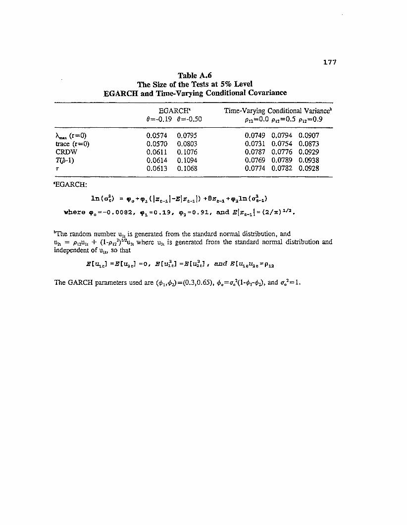
177Table A.6

The Size of the Tests at 5% Level EGARCH and Time-Varying Conditional Covariance

E G A R C H * Time-Varying Conditional Varianceb0=-O.19 0=-O.5O P\i~ o.o Pi2— 0.5 Pi2~ 0.9

(r=0) 0.0574 0.0795 0.0749 0.0794 0.0907trace (r=0) 0.0570 0.0803 0.0731 0.0754 0.0873C R D W 0.0611 0.1076 0.0787 0.0776 0.0929Tip-1) 0.0614 0.1094 0.0769 0.0789 0.0938T 0.0613 0.1068 0.0774 0.0782 0.0928

• E G A R C H :

I n (oa) = q>„ + (| zt_x ] |) + 0 2 .3. + <pal n (

w h e r e <pQ = -0 . 0082, ^ = 0 . 1 9 , <p2 = 0.91, a n d ^ I z ^ l = (2/it)1/a.

hThe random number u„ is generated from the standard normal distribution, andu2t = Pi2un + (l~Pi22)1/2u3i where u3l is generated from the standard normal distribution andindependent of uU) so that

St u ^ ] = S [ u 3t;] =0, S [ U i t] =JS[Ua3t] , a n d E[xiLtu2t = p12

The G A R C H parameters used tire (< 1,^2) = (0.3,0.65), and <r02=l.

178quarterly U.S. real GNP for 1947:2 to 1991:1. Their estimated asymmetric volatility with 6 - -0.19 does not seem to make much difference from the previous cases with symmetric GARCH models. However, when the asymmetric volatility parameter is increased to 9 = -0.50, the bias of the empirical size becomes larger. In Table A.A.3, another form of GARCH models that also allows for asymmetric impact of volatility innovation—

quadratic GARCH (QGARCH) proposed by Engle (1990), Sentana (1991), and Campbell and Hentschel (1992)— is examined. QGARCH models are more analytically tractable that EGARCH types; particularly, the unconditional variance is explicitly determined. The results are consistent with those of EGARCH model; i.e, asymmetric volatility effects intensify the size distortion.

Although the paper has reported the results under the assumption that the conditional covariances are zero for all t, E [e ^ | ] = 0, i^j, it also experiments with time-varying conditional covariances in the second part of Table A.6. For simplicity, only the bivariate system (AM2) is studied. The conditional covariance is E [ ene* | ] - P ^ xP tx> where p12t is the conditional correlation. Assume that the conditional correlation is constant over time, i.e., Pnt=Pn f°r all t, as in Bollerslev (1990). This specification of the time-constant conditional correlation is adopted so that only one parameter p12 is controlled. The data uu is generated from the standard normal distribution, and Uj, = p2tuu + (l-p,22) ,/2u3t where u3t is

179generated from the standard normal distribution and independent of ult. Thus

•E[ult] =E[uzt] =0, E[uf;t] =E[uit] =1, and 1'3[ultu2tl = p12.

The second part of Table A.6 reports the results with pn = 0, 0.5, and 0.9. A large pn is very likely in practice. For example, in Kroner and Sultan (1993), estimated pn is ranged from 0.96 to 0.99 for weekly spot and futures foreign currency series. The GARCH parameters used are (0t, <f>2) = (0.3, 0.65), 0O = a02( 1-0^02), and a02 = 1. It is shown that the size distortion increases with p12, even if the GARCH model is not degenerate or integrated and even if it should not matter in theory as the Johansen procedure allows for time-varying conditional covariances.6

It is probable that at least one of the series employed in a system is not (nearly) degenerate and integrated, though the other series are. Table A.7 examines the size of the tests when this is the case. For the residual-based tests, it is particularly interesting to distinguish the case where the dependent variable in the cointegrating regression has an integrated GARCH from the cases otherwise. In Table A.7,

6It is seen from an experiment that when there is no GARCH the empirical size is virtually equal to the nominal size for all values of p12 = 0, 0.5, and 0.9, as expected in theory since the Johansen procedure allows for non-zero conditional covariance. This is not the case when there is GARCH even if the GARCH is not integrated.

180


N = 2, 3; T = 100, 1000

N 2 3 3

(0.3,0.7) (0.3,0.7) (0.3,0.7)($ 2 1»$22^ (0.3,0.65) (0.3,0.65) (0.3,0.7)($ 3 1 > $32) (0.3,0.65) (0.3,0.65) (0.3,0.65)

Panel A: T = '.100

Case A B A B A B

> W (r=0) 0.1393 0.1393 0.1547 0.1547 0.3479 0.3479trace (r=0) 0.1309 0.1309 0.1485 0.1485 0.3369 0.3369C R D W 0.1723 0.0801 0.1485 0.0704 0.1956 0.0738Tip-1) 0.2432 0.0849 0.2089 0.0753 0.2642 0.0797T 0.2519 0.0861 0.2211 0.0784 0.2796 0.0815

Panel B: T = 1000

Case A B A B A B

(r== 0) 0.2099 0.2099 0.2388 0.2388 0.9271 0.9271trace (r=0) 0.1991 0.1991 0.2157 0.2157 0.9073 0.9073C R D W 0.7616 0.0693 0.7109 0.0738 0.8948 0.0709Tip-1) 0.9075 0.0754 0.8735 0.0817 0.9476 0.0811T 0.9123 0.0758 0.8790 0.0834 0.9510 0.0809

Case A is when xu is the dependent variable in cointegrating regressions in computing the regression-based statistics ( C R D W , Tip-1), r). Case B is when xNl is the dependent variable. A x u= e lt has a conditional variance of an integrated G A R C H , while AxNt= e Nl has a G A R C H that are not integrated. and ai02=l, i = l,..,N.

181Axlt=elt has a conditional variance of an integrated GARCH with (0n#0i2)= (0.3,0.7), while AxNt=eNt has a GARCH that is notintegrated with (0n1,0n2) = (O.3, 0.65), = (l-0iI-0i?), and or02 =1, i = 1, ... , N. Case A is when xlt is the dependent variable in cointegrating regressions in computing the regression-based statistics (CRDW, T(p-l) , t ) , and Case B is when xNt is the dependent variable.

The results generally show that if the dependent variable in the cointegrating regression is not degenerate and not integrated (Case B), the performance of the Johansen tests is worse than the DF and CRDW tests. The reason may be that the full information maximum likelihood method is more easily contaminated by the "problem" (degeneracy and integratedness) incurred by one of theseries in the system than the residual-based methods such as the DF and CRDW tests. However, if the dependent variable has an integrated GARCH and thus degenerate (Case A), then the residual-based tests perform much worse than in Case B. Again, the problem is more serious for larger sample.

A.3.2 Fractional CointegrationSince cointegration can be considered a particular case

of fractional cointegration, results for latter are likely to be similar to the former. However, the GPH and MRR statistics are robust to variance nonstationarity as aforementioned; accordingly, the GARCH effects should be smaller less the

182cointegration tests. This argument is supported by results shown in Table A.8. It indicates that the size distortion problem for the GPH test and MRR is less serious than that of the cointegration tests. For example, for 0,=O.3, 0,+02=O.999, and T=1000, the size of GPH test is 12.2% (»>=0.50), MRR is 5.2% (Andrew's method), while trace statistic is 13.5%. To be more specific, while the GPH test is moderately biased by the nearly IGARCH process, the effect on the MRR statistic is very small. Moreover, for the GPH test, results show that smaller values of v (not greater than 0.5) should be chosen if the processes follow a IGARCH. For the MRR statistic, it is worth noting that when 0,=Q.3, the Andrew method choosing g performs worse than other values of g, even for g=0. For example, when (01/02) ~ (0.3,0.699) and T=100, the sizes are 0.097 if q is selected by the Andrews method, but only 0.051 and 0.052 for g=0 and 25, respectively. Also, generally, g=0 gives slightly higher size distortion than g=l, 5, 10, and 25.

A.4 Conclusions

This appendix examines the finite sample performance of cointegration and fractional cointegration tests under the presence of GARCH. The cointegration tests tend to over-reject the null hypothesis of no cointegration in favor of finding cointegration too often in the presence of GARCH errors, especially when 0O is close to zero, 0!+02 is close to unity, and 0, is large. Generally the problem becomes more serious as

183

Table A.8T h e Size of the Tests at 5% Level: Fractional Cointegration Tests

_______________ N = 2; 4>„ = g02(l-<&1 2)> <ra2 = 1_______________T 100 1000 100 1000 100 1000 100 1000

Panel A

(*„&) (0.3,0.6) (0.3,0.65) (0.3,0.699) (0.3,0.7)

G H P Test^=0.40 0.0490 0.0482 0.0515 0.0513 0.0591 0.0770 0.0865 0.3492

0.45 0.0515 0.0590 0.0547 0.0747 0.0667 0.0991 0.0974 0.36840.50 0.0586 0.0612 0.0614 0.0780 0.0741 0.1221 0.1145 0.43750.55 0.0612 0.0593 0.0627 0.0833 0.0814 0.1349 0.1231 0.48120.60 0.0658 0.0761 0.0652 0.1047 0.0829 0.1519 0.1344 0.52070.65 0.0657 0.0817 0.0656 0.1013 0.0864 0.1627 0.1405 0.50240.70 0.0662 0.0856 0.0684 0.1013 0.0911 0.1782 0.1497 0.5095

M R S/= 0 0.0523 0.0518 0.0505 0.0518 0.0505 0.0493 0.0580 0.0580

1 0.0421 0.0497 0.0424 0.0488 0.0388 0.0423 0.0356 0.03565 0.0335 0.0450 0.0324 0.0410 0.0262 0.0318 0.0127 0.012710 0.0337 0.0422 0.0306 0.0376 0.0267 0.0241 0.0075 0.007525 0.0528 0.0397 0.0530 0.0314 0.0524 0.0182 0.0506 0.0506A 0.0897 0.0654 0.0867 0.0626 0.0971 0.0520 0.1326 0.1009

Panel B

(*„*a) (0.1,0.8) (0.1,0.85) (0.1,0.899) (0.1,0.9)

G P H Test^=0.40 0.0470 0.0461 0.0476 0.0490 0.0494 0.0728 0.0491 0.1543

0.45 0.0493 0.0480 0.0496 0.0513 0.0512 0.0840 0.0515 0.18020.50 0.0526 0.0551 0.0503 0.0586 0.0539 0.0920 0.0543 0.20070.55 0.0521 0.0542 0.0529 0.0555 0.0547 0.0912 0.0550 0.20550.60 0.0548 0.0513 0.0540 0.0589 0.0532 0.0944 0.0539 0.21170.65 0.0546 0.0546 0.0539 0.0571 0.0553 0.0979 0.0564 0.21620.70 0.0536 0.0548 0.0527 0.0616 0.0531 0.1014 0.0551 0.2199

M R S/= 0 0.0503 0.0525 0.0508 0.0501 0.0500 0.0420 0.0506 0.0448

1 0.0470 0.0521 0.0458 0.0496 0.0471 0.0413 0.0468 0.03935 0.0472 0.0525 0.0448 0.0494 0.0420 0.0379 0.0438 0.030010 0.0424 0.0506 0.0424 0.0484 0.0383 0.0341 0.0354 0.019425 0.0471 0.0483 0.0473 0.0443 0.0460 0.0254 0.0444 0.0007A 0.0469 0.0520 0.0469 0.0491 0.0466 0.0412 0.0460 0.0363

184T increases. The White heterokedasticity correction may improve the size of the DF test in the presence of GARCH, but only with very poor power performance. The Johansen trace test is generally found to have smaller size distortion than the Johansen maximum eigenvalue test. The size bias of the cointegration tests in the presence of GARCH also increases moderately when uit follows the Student-t distribution instead of the normal distribution, when the GARCH is of EGARCH form, and when the conditional covariances are time-varying.

The size of the GPH test is also affected by the GARCH effects, but the bias is smaller than the cointegration tests. A smaller v is suggested if the processes follow a IGARCH. The MRR statistic is shown to fairly robust to the GARCH innovations.

In conclusion, fractional cointegration tests, which allow noninteger differences, are evinced to be more robust to GARCH innovations than cointegration tests. Hence, results given by fractional cointegration tests are more reliable than conventional cointegration tests.

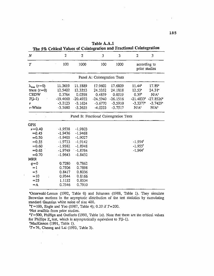
185

Table A.A.lThe 5% Critical Values of Cointegration and Fractional Cointegration

N 2 2 3 3 2 3

T 100 1000 100 1000 according to prior studies

Panel A: Cointegration Tests

> w (r=0) 11.3619 11.1889 17.9602 17.6809 11.44* 17.89*trace (r=0) 12.5402 12.3353 24.3352 24.1818 12.53* 24.31*C R D W 0.3764 0.0398 0.4859 0.0519 0.39b N / A cT(p-1) -19.4660 -20.4922 -24.5940 -26.1516 -21.4833d -27.8526dT -3.2123 -3.1624 -3.6770 -3.5910 -3.3377° -3.7429°r-White -3.5680 -3.3655 -4.0333 -3.7517 N/A° N/A°

Panel B: Fractional Cointegration Tests

G P Hj>=0.40 -1.9538 -1.9803=0.45 -1.9436 -1.9468=0.50 -1.9405 -1.9027=0.55 -1.9733 -1.9142 -1.954f=0.60 -1.9582 -1.8948 -1.955f=0.65 -1.9749 -1.8784 -1.964f=0.70 -1.9643 -1.8432

M R Rq= 0 0.7280 0.7862= 1 0.7506 0.7898= 5 0.8417 0.8036= 10 0.9344 0.8166=25 1.1152 0.8534= A 0.7546 0.7910

*Osterwald-Lenum (1992, Table 0) and Johansen (1988, Table 1). They simulate Brownian motions in the asymptotic distribution of the test statistics by cumulating standard Gaussian white noise of size 400.^ = 1 0 0 , Engle and Yoo (1987, Table 4); 0.20 if 7=200.'Not availble from prior studies.dT=500, Phillips and Outliaris (1990, Table la). Note that these are the critical values for Phillips Z 0 test, which is asymptotically equivalent to T(p-1).'MacKinnon (1991, Table 1).fT = 76, Cheung and Lai (1993, Table 3).

186Table A.A.2

The Size of the Tests at 5% Level QGARCH

N = 2; T = 100

(0 (0.3,0.65) (0.3,0.69) (0.1,0.85) (0.1,0.89)

b 0.1 0.5 0.1 0.5 0.1 0.5 0.1 0.5

> w (r=0) 0.0753 0.0770 0.0882 0.0997 0.0588 0.0596 0.0651 0.0694trace (r=0) 0.0718 0.0748 0.0843 0.0985 0.0547 0.0574 0.0639 0.0694C R D W 0.0791 0.0861 0.0859 0.1265 0.0564 0.0562 0.0590 0.0601Tip-1) 0.0788 0.0856 0.0878 0.1294 0.0564 0.0552 0.0604 0.0585r 0.0767 0.0861 0.0872 0.1297 0.0564 0.0554 0.0601 0.0588

Q G A R C H : cr2 = 4>a + -Me^-b)2 + tf>2<rM 2. If b=0, then G A R C H .The unconditional variance, <r02, is set equal to 1;where <r02 = (< 0+^ib2)/(l-(<j!>l+i^)). (See Campbell and Hentschel (1992))

VITA

Born in Hong Kong, Yiuman Tse received his Bachelor of Science (Mechanical Engineering) from University of Hong Kong and Master of Business Administration from State University of New York at Binghamton. His areas of interest include investment, time series analysis, and international finance. Mr. Tse will be employed as a visiting assistant professor by Louisiana State University in August 1994.

187

DOCTORAL EXAMINATION AND DISSERTATION REPORT

Candidate: Yiuman Tse

Major Field: Business Administration (Finance)

Title of Dissertation: Three Essays on Short-Term InterestRate Futures

Approved:

EXAMINING COMMITTEE:

Date of Examination:

May 16, 1994

three essays on short-term interest rate futures

Documents