thursday morning growth modelling in mplus
TRANSCRIPT
1
Thursday Morning
Growth Modelling in MplusUsing a set of repeated continuous measures of bodyweight
2
Growth modelling – Continuous Data
• Mplus model syntax refresher
• ALSPAC
• Confirmatory Factor Analysis (CFA)
• Latent Growth Modelling (LGM)
– Path diagrams
– Models of increasing complexity
– Adding covariates
– Extension to parallel processes
– Practical

3
Mplus model syntax
A quick refresher

4
Model statements: BY / WITH / ON
• X is correlated WITH YX with Y;
• Y (outcome) is regressed on X (predictor)Y on X;
• F (the factor) is measured BY Y1 Y2 Y3F by Y1 Y2 Y3;
YX
YX
y3y2y1
F

5
Variable means
• Stuff in a square bracket is a mean/intercept:[wt_7 wt_9 wt_11];
• It’s just the same to say:[wt_7];
[wt_9];
[wt_11];

6
Variances
• No bracket, then it’s a variance / residual variance:wt_7;
wt_9;
wt_11;
• Orwt_7 wt_9 wt_11;

7
Parameter equality constraints
• Three residual variances constrained to be equal:wt_7 (1);
wt_9 (1);
wt_11 (1);
• Three intercept constrained to be equal:[wt_7] (2);
[wt_9] (2);
[wt_11] (2);

8
Parameter equality constraints
• Three residual variances constrained to be equal:wt_7 (fixvar);
wt_9 (fixvar);
wt_11 (fixvar);
• Three intercept constrained to be equal:[wt_7] (fixmean);
[wt_9] (fixmean);
[wt_11] (fixmean);
9
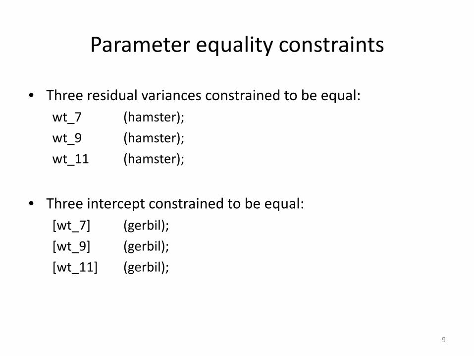
Parameter equality constraints
• Three residual variances constrained to be equal:wt_7 (hamster);
wt_9 (hamster);
wt_11 (hamster);
• Three intercept constrained to be equal:[wt_7] (gerbil);
[wt_9] (gerbil);
[wt_11] (gerbil);

10
Fixing parameters
• Constraining a covariance to be zero:X with Y@0;
• Constraining a mean to be zero:[wt_7@0];
• Constraining a variance to be zero:i@0;

Where’s Avon to, my luvver?trans: Where is Avon?
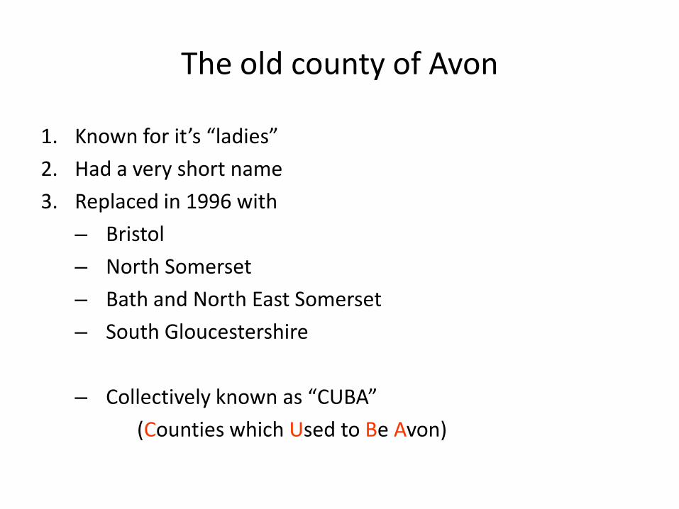
The old county of Avon
1. Known for it’s “ladies”
2. Had a very short name
3. Replaced in 1996 with
– Bristol
– North Somerset
– Bath and North East Somerset
– South Gloucestershire
– Collectively known as “CUBA”
(Counties which Used to Be Avon)

What is ALSPAC?
• “Avon Longitudinal Study of Parents and Children” AKA Children of the Nineties
• Cohort study of ~14,000 children and their parents, based in South-West England
• Eligibility criteria: Mothers had to be resident in Avon and have an expected date of delivery between April 1st 1991 and December 31st 1992
• Population-Based Prospective Birth-Cohort

What data does ALSPAC have?
• Self completion questionnaires
– Mothers, Partners, Children, Teachers
• Hands on assessments
– 10% sample tested regularly since birth
– Yearly clinics for all since age 7
• Data from external sources
– SATS from LEA, Child Health database
• Biological samples
– DNA / cell lines

1515
Bodyweight example
• Bodyweight measurements from ALSPAC clinic
• Three time points: 7, 9, 11 years
• N = 3,883 with complete data
• Summary statistics:-
MeansWT7 WT9 WT11
25.532 34.219 43.214
CovariancesWT7 WT9 WT11
WT7 18.365
WT9 27.543 49.787
WT11 35.565 63.250 92.845

1616
What the data looks like - v1
Age (years)
Wei
ght (
kg)

1717
What the data looks like – v2
Weight
Age
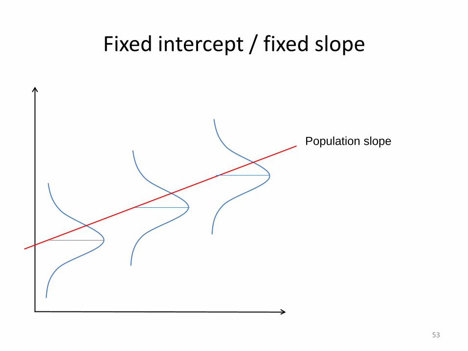
Population slope
Repeated measuresNormally distributed with increasing spread

18
Confirmatory Factor Analysis
y3y2y1
ε1 ε2 ε3
Of interest here are the loadings (λi), and the uniquenesses (εi) or residuals which have error variances σi
2
The interpretation of the factor is governed by the way it loads on the observed data.
λ1 λ2 λ3
F

19
Confirmatory Factor Analysis
y3y2y1
ε1 ε2 ε3Each component is a simple regression equation:
Y1 = λ1F + ε1
Except that F is latent rather than observed
In CFA we do not model the mean structure – hence there is no intercept in the above regression equation
Therefore CFA can be carried out using standardized measures
λ1 λ2 λ3
F

20
CFA - Covariance structure
y3y2y1
ε1 ε2 ε3
The data to be modelled consists of a covariance matrix
λ1 λ2 λ3
F
Var(y1)
Cov(y1,y2) Var(y2)
Cov(y1,y3) Cov(y1,y3) Var(y3)
We can write these six items in terms of the 7 parameters of interest:-
λ1 λ2 λ3 ε1 ε2 ε3 Var(F)
To many unknowns (under-identified) so we must apply a constraint.

21
CFA - in Mplus
y3y2y1
ε1 ε2 ε3Model:
F by y1* y2 y3;F@1;
The factor F is measured by the set of items y1-y3
Here we have freed the estimation of the first loading and constrained the factor variance
The Mplus default is to fix the first loading and estimate the variance of F. It’s just a matter of preference.
λ1 λ2 λ3
F

Now on to growth models
Not just for things that grow!
(Although things that don’t change at all
can be boring to model)
23
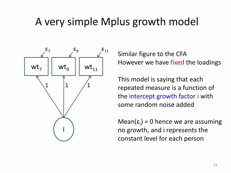
A very simple Mplus growth model
wt11wt9wt7
ε7 ε9 ε11 Similar figure to the CFAHowever we have fixed the loadings
This model is saying that each repeated measure is a function of the intercept growth factor i with some random noise added
Mean(εi) = 0 hence we are assuming no growth, and i represents the constant level for each person
1 1 1
i

24
The Mean Structure
wt11wt9wt7
ε7 ε9 ε11We can write the equations in the same way as for CFA but there is an additional term as the Y’s are not standardized for these models:
wt7 = α7 + i + ε7
wt9 = α9 + i + ε9
wt11 = α11 + i + ε11
1 1 1
We have 4 things to estimate α7,α9,α11 & E(i) but only 3 measures: the means of wt7 wt9 wt11
Standard convention to fix intercepts to zero and just estimate mean of the growth factor(s)
i

25
Degrees of Freedom
wt11wt9wt7
ε7 ε8 ε11Covariance Structure
Covariance matrix of Y gives us 6 terms: 3 cov’s and 3 vars.
Here we are estimating 4 things:3 residual variances and the var(i)
Over-identified -> Good
Mean Structure
We have 3 terms – means of Y’sWe are estimating 1 thing: mean(i)Over-identified -> Good
1 1 1
You can’t pool the d.f.- estimate less in the mean structure to allow a more complex covariance structure
i

2626
Linear Growth Model - Degrees of Freedom
wt11wt9wt7
ε7 ε9 ε11
1 1 1
2 4
i s
Covariance Structure
Covariance matrix of wt gives 6 terms: 3 cov’s and 3 vars.
Here we are estimating 4 things:A residual variance and the covariance
matrix for the growth factorsOver-identified
Mean Structure
We have 3 terms – means of wt’sWe are estimating 2 things: mean(i) and mean(s)Over-identified

2727
Linear Growth Model - Degrees of Freedom
wt11wt9wt7
ε7 ε9 ε11Covariance Structure
What if we relaxed the residual variance constraint?
Var(i), Var(s), Cov(i,s), (σ7)2, (σ9)2, (σ11)2
No d.f. spare -> Just identified
For 3 time points it is not possible to estimate more than 6 var/cov parameters.
Even if there are d.f. going spare in the mean structure model
1 1 1
2 4
i s

28
Aim - Compare 5 models of bodyweight
• Fixed intercept / no slope
• Random intercept / no slope
• Fixed intercept / fixed slope
• Random intercept / fixed slope
• Random intercept / random slope
WHY?
• Statistical models based on assumptions
• Violated assumptions -> incorrect results
• Need to capture between and within person variability in growth as accurately as possible
• Leads to correct inferences when incorporating covariates

30
[1] Fixed intercept / no slope
31
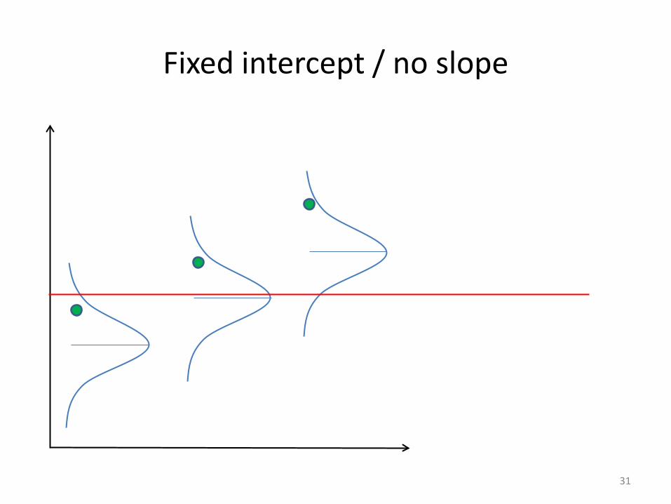
Fixed intercept / no slope

32
Fixed intercept / no slope
Assumes residuals (errors) have variance which is constant over time+ adjacent residuals areuncorrelated

33
Fixed intercept / no slope
wt11wt09wt07
ε ε ε
Single growth factorEqual residual variances
1 1 1
model:i | wt_07@0 wt_09@2 wt_11@4;wt_07 (1);wt_09 (1);wt_11 (1);i@0;
Which is Mplus shorthand for:
i by wt_07@1 wt_09@1 wt_11@1;[wt_07@0 wt_09@0 wt_11@0 i];wt_07 (1)wt_09 (1)wt_11 (1);i@0;
i

34
Fixed intercept / no slope
wt11wt09wt07
ε ε ε
Single growth factorEqual residual variances
1 1 1
model:i | wt_07@0 wt_09@2 wt_11@4;wt_07 (1);wt_09 (1);wt_11 (1);i@0;
Which is the same as:
i by wt_07@1 wt_09@1 wt_11@1;[wt_07@0 wt_09@0 wt_11@0 i];wt_07 (1)wt_09 (1)wt_11 (1);i@0; Loadings
are fixed
i

35
Fixed intercept / no slope - resultsMODEL RESULTS
Two-TailedEstimate S.E. Est./S.E. P-Value
I |WT_07 1.000 0.000 999.000 999.000WT_09 1.000 0.000 999.000 999.000WT_11 1.000 0.000 999.000 999.000
MeansI 34.322 0.095 360.167 0.000
InterceptsWT_07 0.000 0.000 999.000 999.000WT_09 0.000 0.000 999.000 999.000WT_11 0.000 0.000 999.000 999.000
VariancesI 0.000 0.000 999.000 999.000
Residual VariancesWT_07 105.782 1.386 76.319 0.000WT_09 105.782 1.386 76.319 0.000WT_11 105.782 1.386 76.319 0.000

36
Fixed intercept / no slope - resultsMODEL RESULTS
Two-TailedEstimate S.E. Est./S.E. P-Value
I |WT_07 1.000 0.000 999.000 999.000WT_09 1.000 0.000 999.000 999.000WT_11 1.000 0.000 999.000 999.000
MeansI 34.322 0.095 360.167 0.000
InterceptsWT_07 0.000 0.000 999.000 999.000WT_09 0.000 0.000 999.000 999.000WT_11 0.000 0.000 999.000 999.000
VariancesI 0.000 0.000 999.000 999.000
Residual VariancesWT_07 105.782 1.386 76.319 0.000WT_09 105.782 1.386 76.319 0.000WT_11 105.782 1.386 76.319 0.000
(25.532 + 34.219 + 43.214)/3
All the variance in the dataset becomes residual variance (error) as nothing has been explained

37
Fixed intercept / no slope - residuals
MeansWT_07 WT_09 WT_1125.532 34.219 43.214
Model Estimated Means/Intercepts/Thresholds
WT_07 WT_09 WT_1134.322 34.322 34.322
Residuals for Means/Intercepts/Thresholds
WT_07 WT_09 WT_11 -8.790 -0.103 8.893

38
Fixed intercept / no slope - residuals
CovariancesWT_07 WT_09 WT_11
WT_07 18.365WT_09 27.543 49.787WT_11 35.565 63.250 92.845
Model Estimated Covariances/Correlations/Residual Correlations
WT_07 WT_09 WT_11WT_07 105.782WT_09 0.000 105.782WT_11 0.000 0.000 105.782
Residuals for Covariances/Correlations/Residual Correlations
WT_07 WT_09 WT_11WT_07 -87.418WT_09 27.543 -55.995WT_11 35.565 63.250 -12.938
39
[2] Random intercept / no slope

40
Random intercept / no slope
Same population mean

41
Random intercept / no slope
Each individual giventheir own mean level

42
Random intercept / no slope
Model assumes individual means normally distributed about global mean

43
Random intercept / no slope
Assumes residuals are N(0,σ²) about individual intercepts, variability constant over time+ adjacent residuals uncorrelated

44
Random intercept / no slope
wt11wt09wt07
ε ε ε
Single growth factorEqual residual variances
1 1 1
model:i | wt_07@0 wt_09@2 wt_11@4;wt_07 (1);wt_09 (1);wt_11 (1);
Which is the same as:
i by wt_07@1 wt_09@1 wt_11@1;[wt_07@0 wt_09@0 wt_11@0 i];wt_07 (1);wt_09 (1);wt_11 (1);i;
i
45
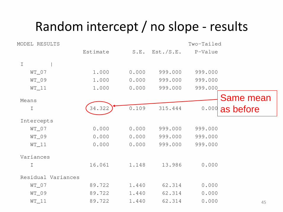
Random intercept / no slope - resultsMODEL RESULTS Two-Tailed
Estimate S.E. Est./S.E. P-Value
I |
WT_07 1.000 0.000 999.000 999.000
WT_09 1.000 0.000 999.000 999.000
WT_11 1.000 0.000 999.000 999.000
Means
I 34.322 0.109 315.444 0.000
Intercepts
WT_07 0.000 0.000 999.000 999.000
WT_09 0.000 0.000 999.000 999.000
WT_11 0.000 0.000 999.000 999.000
Variances
I 16.061 1.148 13.986 0.000
Residual Variances
WT_07 89.722 1.440 62.314 0.000
WT_09 89.722 1.440 62.314 0.000
WT_11 89.722 1.440 62.314 0.000
Same mean as before

46
Random intercept / no slope - resultsMODEL RESULTS Two-Tailed
Estimate S.E. Est./S.E. P-Value
I |
WT_07 1.000 0.000 999.000 999.000
WT_09 1.000 0.000 999.000 999.000
WT_11 1.000 0.000 999.000 999.000
Means
I 34.322 0.109 315.444 0.000
Intercepts
WT_07 0.000 0.000 999.000 999.000
WT_09 0.000 0.000 999.000 999.000
WT_11 0.000 0.000 999.000 999.000
Variances
I 16.061 1.148 13.986 0.000
Residual Variances
WT_07 89.722 1.440 62.314 0.000
WT_09 89.722 1.440 62.314 0.000
WT_11 89.722 1.440 62.314 0.000
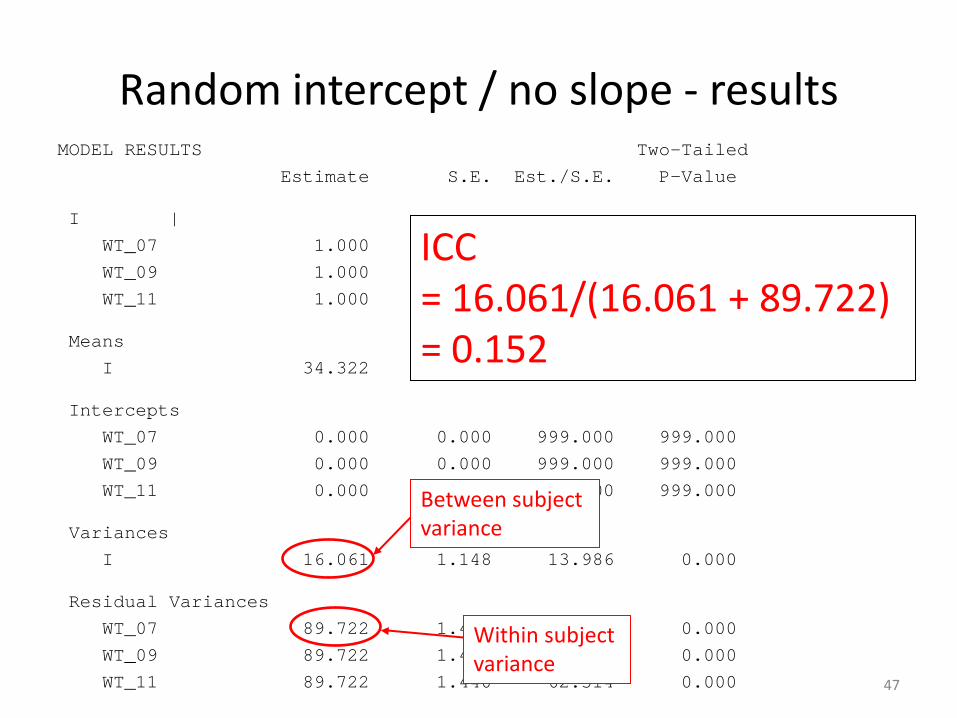
Within subject variance
Between subject variance
47
Random intercept / no slope - resultsMODEL RESULTS Two-Tailed
Estimate S.E. Est./S.E. P-Value
I |
WT_07 1.000 0.000 999.000 999.000
WT_09 1.000 0.000 999.000 999.000
WT_11 1.000 0.000 999.000 999.000
Means
I 34.322 0.109 315.444 0.000
Intercepts
WT_07 0.000 0.000 999.000 999.000
WT_09 0.000 0.000 999.000 999.000
WT_11 0.000 0.000 999.000 999.000
Variances
I 16.061 1.148 13.986 0.000
Residual Variances
WT_07 89.722 1.440 62.314 0.000
WT_09 89.722 1.440 62.314 0.000
WT_11 89.722 1.440 62.314 0.000
Within subject variance
Between subject variance
ICC = 16.061/(16.061 + 89.722) = 0.152

Histogram of intercept factor

Observed data(cases 1-20)
Estimated data(cases 1-20)
50
Random intercept / no slope - residuals
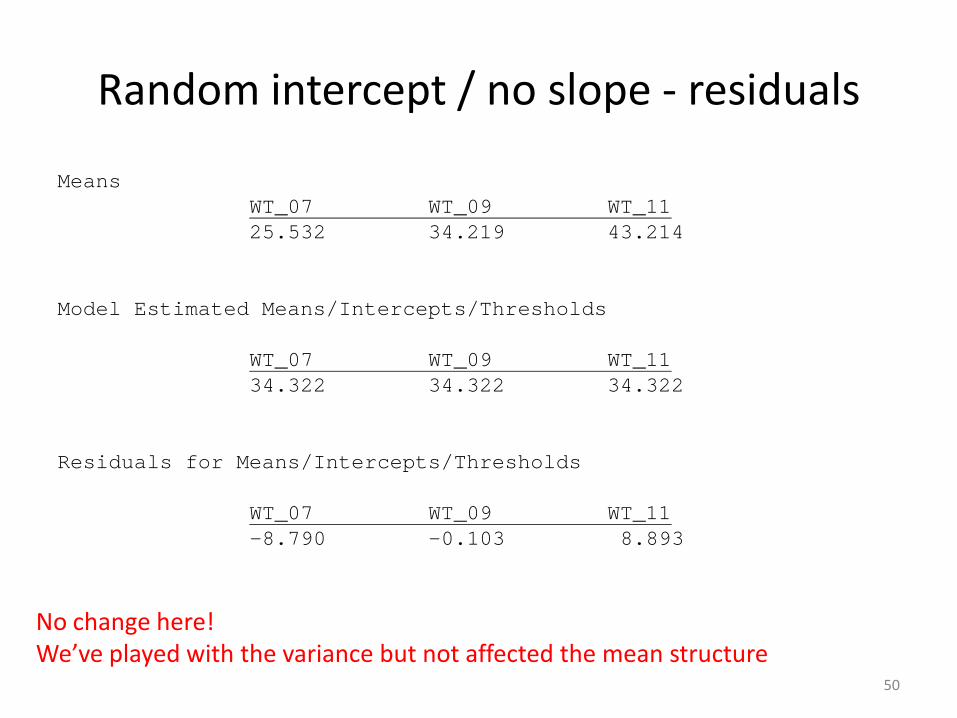
MeansWT_07 WT_09 WT_1125.532 34.219 43.214
Model Estimated Means/Intercepts/Thresholds
WT_07 WT_09 WT_1134.322 34.322 34.322
Residuals for Means/Intercepts/Thresholds
WT_07 WT_09 WT_11 -8.790 -0.103 8.893
No change here!We’ve played with the variance but not affected the mean structure
51
Random intercept / no slope - residuals
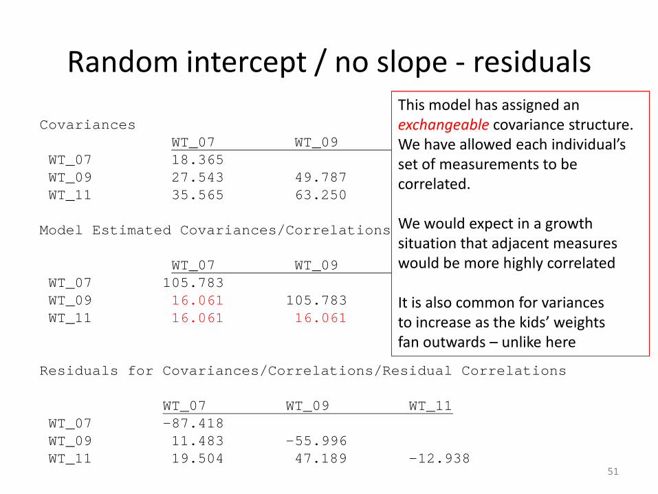
CovariancesWT_07 WT_09 WT_11
WT_07 18.365WT_09 27.543 49.787WT_11 35.565 63.250 92.845
Model Estimated Covariances/Correlations/Residual Correlations
WT_07 WT_09 WT_11WT_07 105.783WT_09 16.061 105.783WT_11 16.061 16.061 105.783
Residuals for Covariances/Correlations/Residual Correlations
WT_07 WT_09 WT_11WT_07 -87.418WT_09 11.483 -55.996WT_11 19.504 47.189 -12.938
This model has assigned an exchangeable covariance structure.We have allowed each individual’s set of measurements to be correlated.
We would expect in a growth situation that adjacent measures would be more highly correlated
It is also common for variancesto increase as the kids’ weightsfan outwards – unlike here

52
[3] Fixed intercept / fixed slope
53
Fixed intercept / fixed slope
Population slope
54
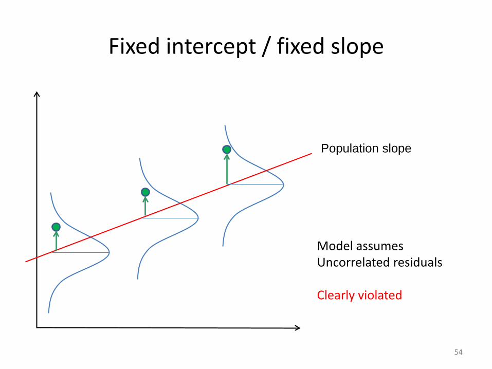
Fixed intercept / fixed slope
Population slope
Model assumes Uncorrelated residuals
Clearly violated
55
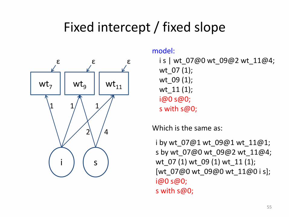
Fixed intercept / fixed slope
wt11wt9wt7
ε ε ε
1 1 1
2 4
model:i s | wt_07@0 wt_09@2 wt_11@4;wt_07 (1);wt_09 (1);wt_11 (1);i@0 s@0;s with s@0;
Which is the same as:
i by wt_07@1 wt_09@1 wt_11@1;s by wt_07@0 wt_09@2 wt_11@4;wt_07 (1) wt_09 (1) wt_11 (1);[wt_07@0 wt_09@0 wt_11@0 i s];i@0 s@0;s with s@0;
i s

5656
Choice of loadings for SLOPE
wt11wt9wt7
ε ε ε
1 1 1
2 4
i s
It is traditional for the intercept factor to have a unit loading on each repeated measure
Here we have used loadings of 0/2/4 for the slope factor since the repeated measures are 2 years apart.
E.g. expected weight at age 11= intercept plus 4*gradient
Alternative loadings for slope would be 7/11/13, 0/24/48, … as long as the relative spacing preserved.
The interpretation of i has now changed

57
Fixed intercept / fixed slope - results
MODEL RESULTS Two-TailedEstimate S.E. Est./S.E. P-Value
<snip>
I WITHS 0.000 0.000 999.000 999.000
MeansI 25.480 0.107 237.416 0.000S 4.421 0.042 106.352 0.000
InterceptsWT_07 0.000 0.000 999.000 999.000WT_09 0.000 0.000 999.000 999.000WT_11 0.000 0.000 999.000 999.000
VariancesI 0.000 0.000 999.000 999.000S 0.000 0.000 999.000 999.000
Residual VariancesWT_07 53.671 0.703 76.318 0.000WT_09 53.671 0.703 76.318 0.000WT_11 53.671 0.703 76.318 0.000
(25.532 + 34.219 + 43.214)/3 - 2*4.421
(43.214 - 25.532)/4
58
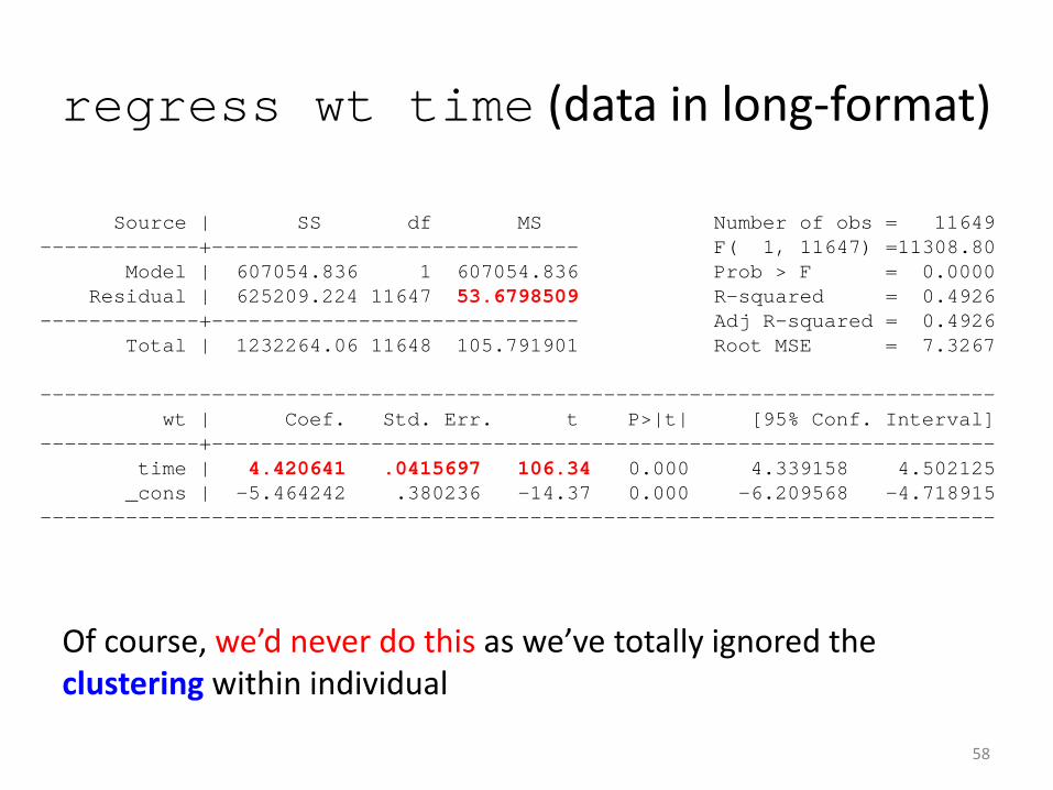
regress wt time (data in long-format)
Source | SS df MS Number of obs = 11649-------------+------------------------------ F( 1, 11647) =11308.80
Model | 607054.836 1 607054.836 Prob > F = 0.0000Residual | 625209.224 11647 53.6798509 R-squared = 0.4926
-------------+------------------------------ Adj R-squared = 0.4926Total | 1232264.06 11648 105.791901 Root MSE = 7.3267
------------------------------------------------------------------------------wt | Coef. Std. Err. t P>|t| [95% Conf. Interval]
-------------+----------------------------------------------------------------time | 4.420641 .0415697 106.34 0.000 4.339158 4.502125_cons | -5.464242 .380236 -14.37 0.000 -6.209568 -4.718915
------------------------------------------------------------------------------
Of course, we’d never do this as we’ve totally ignored the clustering within individual
59
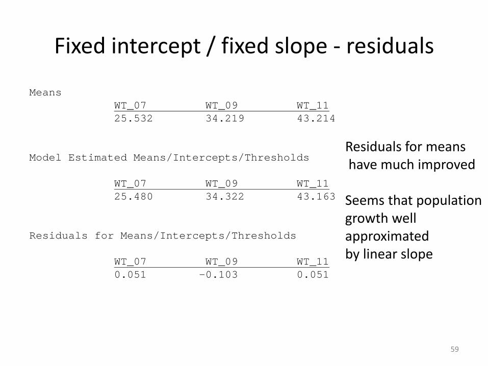
Fixed intercept / fixed slope - residuals
MeansWT_07 WT_09 WT_1125.532 34.219 43.214
Model Estimated Means/Intercepts/Thresholds
WT_07 WT_09 WT_1125.480 34.322 43.163
Residuals for Means/Intercepts/Thresholds
WT_07 WT_09 WT_110.051 -0.103 0.051
Residuals for meanshave much improved
Seems that populationgrowth well approximatedby linear slope
60
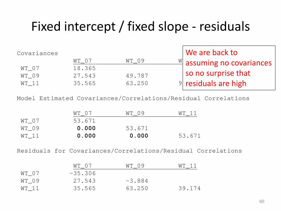
Fixed intercept / fixed slope - residuals
CovariancesWT_07 WT_09 WT_11
WT_07 18.365WT_09 27.543 49.787WT_11 35.565 63.250 92.845
Model Estimated Covariances/Correlations/Residual Correlations
WT_07 WT_09 WT_11WT_07 53.671WT_09 0.000 53.671WT_11 0.000 0.000 53.671
Residuals for Covariances/Correlations/Residual Correlations
WT_07 WT_09 WT_11WT_07 -35.306WT_09 27.543 -3.884WT_11 35.565 63.250 39.174
We are back to assuming no covariancesso no surprise that residuals are high
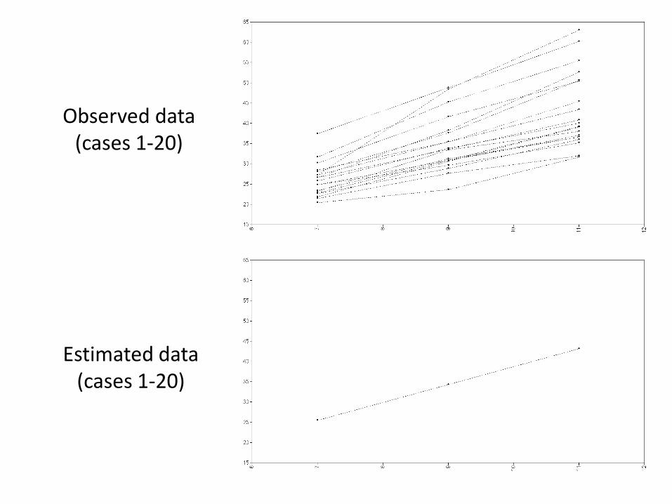
Observed data(cases 1-20)
Estimated data(cases 1-20)

62
[4] Random intercept / fixed slope
63
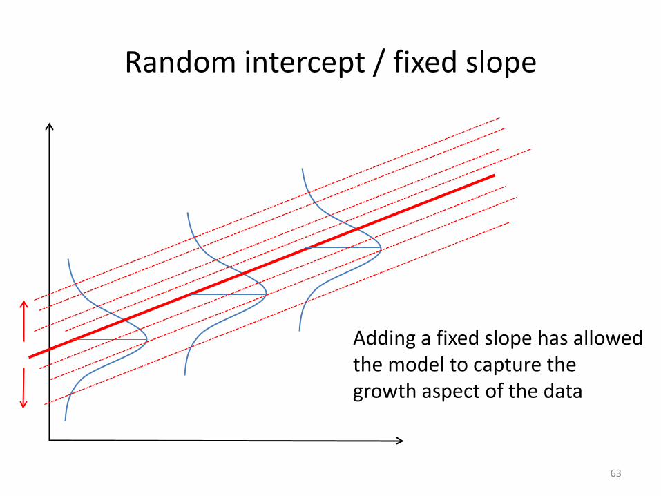
Random intercept / fixed slope
Adding a fixed slope has allowedthe model to capture the growth aspect of the data

64
Random intercept / fixed slope
Residuals are clearly SMALLER(at least for this made-up person)

65
Random intercept / fixed slope
wt11wt9wt7
ε ε ε
1 1 1
1 2
model:i s | wt_07@0 wt_09@2 wt_11@4;wt_07 (1);wt_09 (1);wt_11 (1);i;s@0; ! Slope has no variancei with s@0; ! Hence no covariance
i s

66
Random intercept / fixed slope - resultsMODEL RESULTS Two-Tailed
Estimate S.E. Est./S.E. P-Value
<snip>
I WITHS 0.000 0.000 999.000 999.000
MeansI 25.480 0.115 220.726 0.000S 4.421 0.019 229.218 0.000
InterceptsWT_07 0.000 0.000 999.000 999.000WT_09 0.000 0.000 999.000 999.000WT_11 0.000 0.000 999.000 999.000
VariancesI 42.117 1.045 40.300 0.000S 0.000 0.000 999.000 999.000
Residual VariancesWT_07 11.554 0.185 62.313 0.000WT_09 11.554 0.185 62.313 0.000WT_11 11.554 0.185 62.313 0.000
Mean structure unaffected by allowing intercepts to vary
Previous residual variance has now been partitioned
The majority is now due to variation in starting weight

67
Random intercept / fixed slope - residuals
MeansWT_07 WT_09 WT_1125.532 34.219 43.214
Model Estimated Means/Intercepts/Thresholds
WT_07 WT_09 WT_1125.480 34.322 43.163
Residuals for Means/Intercepts/Thresholds
WT_07 WT_09 WT_110.051 -0.103 0.051
No change here!

68
Random intercept / fixed slope - residuals
CovariancesWT_07 WT_09 WT_11
WT_07 18.365WT_09 27.543 49.787WT_11 35.565 63.250 92.845
Model Estimated Covariances/Correlations/Residual Correlations
WT_07 WT_09 WT_11WT_07 53.671WT_09 42.117 53.671WT_11 42.117 42.117 53.671
Residuals for Covariances/Correlations/Residual Correlations
WT_07 WT_09 WT_11WT_07 -35.306WT_09 -14.574 -3.884WT_11 -6.552 21.133 39.174
We are back to anexchangeable covariance structure.
Compared with the random intercept / no slope modelthe estimated covariances are higher and hence corresponding residuals lower

Observed data(cases 1-20)
Estimated data(cases 1-20)
Things are startingto look much better!

70
[5] Random intercept / random slope
(Standard linear growth model)

71
Random intercept / random slope
Allowing slopes to vary allowsindividuals’ lines to more closelyfit their data points
Population slope unaffected

72
Random intercept / random slope
wt11wt9wt7
ε ε ε
1 1 1
1 2
model:i s | wt_07@0 wt_09@2 wt_11@4;wt_07 (1);wt_09 (1);wt_11 (1);i s;i with s;
i s
73
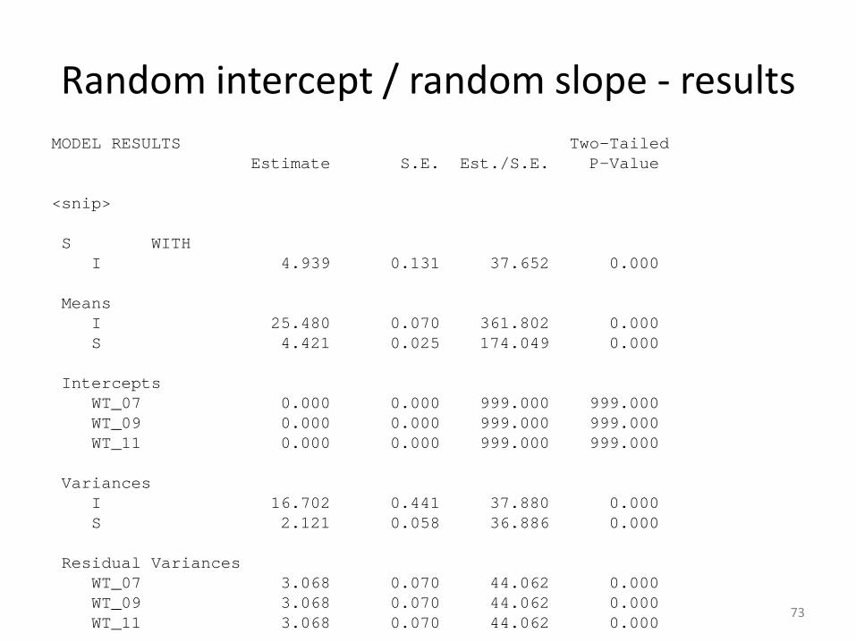
Random intercept / random slope - resultsMODEL RESULTS Two-Tailed
Estimate S.E. Est./S.E. P-Value
<snip>
S WITHI 4.939 0.131 37.652 0.000
MeansI 25.480 0.070 361.802 0.000S 4.421 0.025 174.049 0.000
InterceptsWT_07 0.000 0.000 999.000 999.000WT_09 0.000 0.000 999.000 999.000WT_11 0.000 0.000 999.000 999.000
VariancesI 16.702 0.441 37.880 0.000S 2.121 0.058 36.886 0.000
Residual VariancesWT_07 3.068 0.070 44.062 0.000WT_09 3.068 0.070 44.062 0.000WT_11 3.068 0.070 44.062 0.000

74
Random intercept / random slope - residuals
MeansWT_07 WT_09 WT_1125.532 34.219 43.214
Model Estimated Means/Intercepts/Thresholds
WT_07 WT_09 WT_1125.480 34.322 43.163
Residuals for Means/Intercepts/Thresholds
WT_07 WT_09 WT_110.051 -0.103 0.051
75
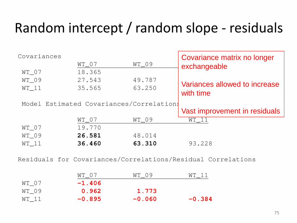
Random intercept / random slope - residuals
CovariancesWT_07 WT_09 WT_11
WT_07 18.365WT_09 27.543 49.787WT_11 35.565 63.250 92.845
Model Estimated Covariances/Correlations/Residual Correlations
WT_07 WT_09 WT_11WT_07 19.770WT_09 26.581 48.014WT_11 36.460 63.310 93.228
Residuals for Covariances/Correlations/Residual Correlations
WT_07 WT_09 WT_11WT_07 -1.406WT_09 0.962 1.773WT_11 -0.895 -0.060 -0.384
Covariance matrix no longerexchangeable
Variances allowed to increasewith time
Vast improvement in residuals

Observed data(cases 1-20)
Estimated data(cases 1-20)
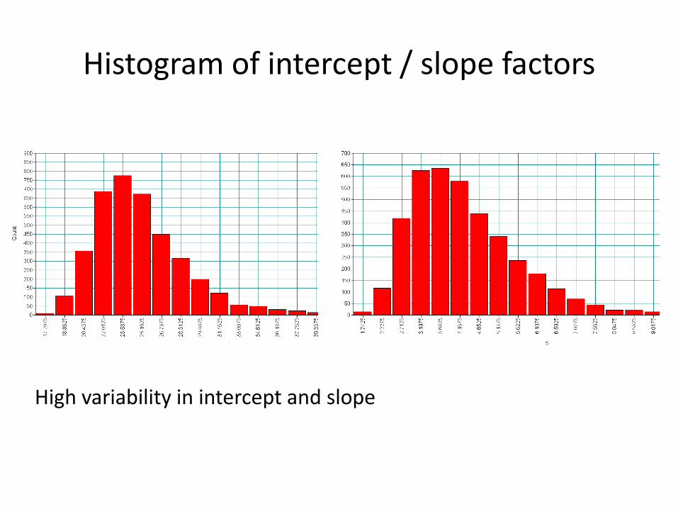
Histogram of intercept / slope factors
High variability in intercept and slope
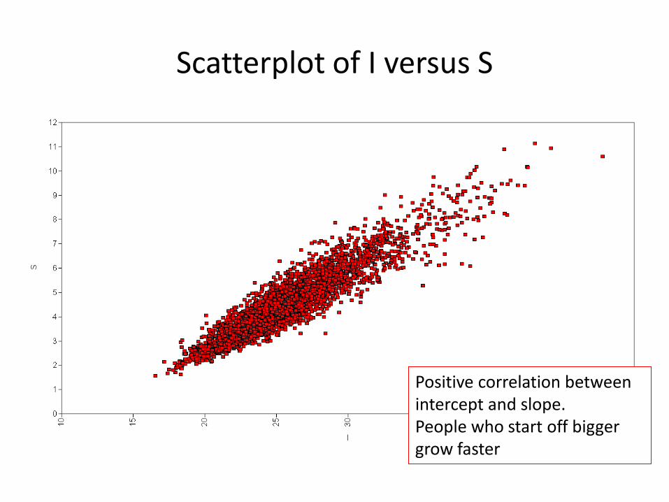
Scatterplot of I versus S
Positive correlation between intercept and slope. People who start off bigger grow faster

79
Results summary – growth factor means
Mean(i) Mean(s)
Fixed intercept / no slope 34.32 (0.095) -
Random intercept / no slope 34.32 (0.109) -
Fixed intercept / fixed slope 25.48 (0.107) 4.42 (0.042)
Random intercept / fixed slope 25.48 (0.115) 4.42 (0.019)
Random intercept / random slope 25.48 (0.070) 4.42 (0.025)
Notice improvement in precision

80
Results summary – (co)variances
Var(i) Var(s) Cov(i,s) Res var
Fixed intercept / no slope - - - 105.8 (1.39)
Random intercept / no slope 16.06 (1.15) - - 89.72 (1.44)
Fixed intercept / fixed slope - - - 53.67 (0.70)
Random intercept / fixed slope 42.12 (1.05) - - 11.56 (0.19)
Random intercept / random slope 16.70 (0.44) 2.12 (0.06) 4.94 (0.13) 3.07 (0.07)
Notice large reduction in error variance
81
Adding Covariates
What explains variation in slope/intercept?

82
Adding covariates
• One aim with these models is to derive a measure or two that summarizes the growth which you can then use as an outcome
• Growth factors become just another variable that you can use as you would an observed measure (outcome/predictor/confounder/mediator….)
• Model for gender is just a bivariate t-test innit?
wt11wt9wt7
ε7 ε9 ε11
1 1 1
2 4
i s
Gender
BWT
83
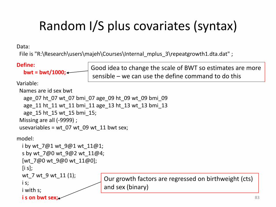
Random I/S plus covariates (syntax)Data:File is "R:\Research\users\majeh\Courses\Internal_mplus_3\repeatgrowth1.dta.dat" ;
Define:bwt = bwt/1000;
Variable:Names are id sex bwt
age_07 ht_07 wt_07 bmi_07 age_09 ht_09 wt_09 bmi_09 age_11 ht_11 wt_11 bmi_11 age_13 ht_13 wt_13 bmi_13 age_15 ht_15 wt_15 bmi_15;
Missing are all (-9999) ; usevariables = wt_07 wt_09 wt_11 bwt sex;
model:i by wt_7@1 wt_9@1 wt_11@1;s by wt_7@0 wt_9@2 wt_11@4;[wt_7@0 wt_9@0 wt_11@0];[i s];wt_7 wt_9 wt_11 (1);i s;i with s;i s on bwt sex;
Good idea to change the scale of BWT so estimates are moresensible – we can use the define command to do this
Our growth factors are regressed on birthweight (cts) and sex (binary)
84
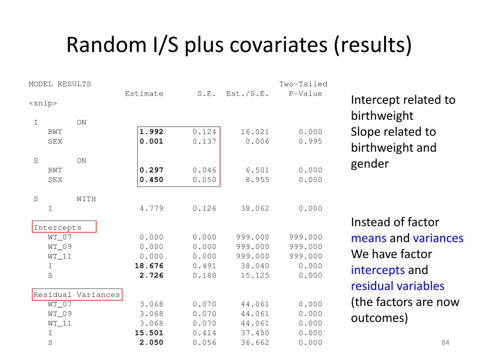
Random I/S plus covariates (results)MODEL RESULTS Two-Tailed
Estimate S.E. Est./S.E. P-Value<snip>
I ONBWT 1.992 0.124 16.021 0.000SEX 0.001 0.137 0.006 0.995
S ONBWT 0.297 0.046 6.501 0.000SEX 0.450 0.050 8.955 0.000
S WITHI 4.779 0.126 38.062 0.000
InterceptsWT_07 0.000 0.000 999.000 999.000WT_09 0.000 0.000 999.000 999.000WT_11 0.000 0.000 999.000 999.000I 18.676 0.491 38.040 0.000S 2.726 0.180 15.125 0.000
Residual VariancesWT_07 3.068 0.070 44.061 0.000WT_09 3.068 0.070 44.061 0.000WT_11 3.068 0.070 44.061 0.000I 15.501 0.414 37.450 0.000S 2.050 0.056 36.662 0.000
Instead of factor means and variancesWe have factorintercepts andresidual variables(the factors are nowoutcomes)
Intercept related tobirthweightSlope related tobirthweight and gender

85
Mis-specified model results:-
I on bwt I on sex S on bwt S on sex
Random intercept / random slope1.992(0.12)
0.001(0.14)
0.297(0.05)
0.450(0.05)
Random intercept / fixed slope2.586(0.19)
0.901(0.21)
- -
Random intercept / no slope2.586(0.19)
0.901(0.21)
- -
Failure to allow slopes to vary forces other aspects of the measurement model to compensate
Consequently we can make incorrect conclusions about effect of gender

Model extension
Parallel models for height and weight

Parallel model of weight and height
wt11wt09wt07
ε ε ε
1 1 1
1 2
wi ws
ht11ht09ht07
η η η
1 1 1
1 2
hi hs
• In addition to estimating
– Mean and variance of I/S
– Covariance between I and S
• We can examine how growth factors
covary between the two processes, e.g.
– cov(wi, hi), cov(ws, hi) …
• We could even regress ws on hi
Weight
Height

What about degrees of freedom?
wt11wt09wt07
ε ε ε
1 1 1
1 2
wi ws
ht11ht09ht07
η η η
1 1 1
1 2
hi hs
• Don’t panic, we have plenty now!
• 6 repeated measures means
6+5+4+3+2 = 15 degrees of freedom
• i.e. more than if you modelled the
two processes separately
Let’s sweep empirical identification under
the carpet for now
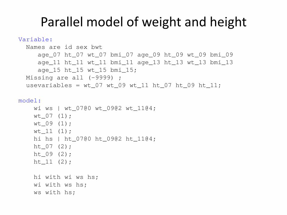
Parallel model of weight and heightVariable:
Names are id sex bwtage_07 ht_07 wt_07 bmi_07 age_09 ht_09 wt_09 bmi_09age_11 ht_11 wt_11 bmi_11 age_13 ht_13 wt_13 bmi_13age_15 ht_15 wt_15 bmi_15;
Missing are all (-9999) ;usevariables = wt_07 wt_09 wt_11 ht_07 ht_09 ht_11;
model:wi ws | wt_07@0 wt_09@2 wt_11@4;wt_07 (1);wt_09 (1);wt_11 (1);hi hs | ht_07@0 ht_09@2 ht_11@4;ht_07 (2);ht_09 (2);ht_11 (2);
hi with wi ws hs;wi with ws hs;ws with hs;
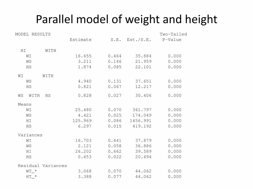
Parallel model of weight and heightMODEL RESULTS Two-Tailed
Estimate S.E. Est./S.E. P-Value
HI WITHWI 16.655 0.464 35.884 0.000WS 3.211 0.146 21.959 0.000HS 1.874 0.085 22.101 0.000
WI WITHWS 4.940 0.131 37.651 0.000HS 0.821 0.067 12.217 0.000
WS WITH HS 0.828 0.027 30.406 0.000
MeansWI 25.480 0.070 361.797 0.000WS 4.421 0.025 174.049 0.000HI 125.969 0.086 1456.991 0.000HS 6.297 0.015 419.192 0.000
VariancesWI 16.703 0.441 37.879 0.000WS 2.121 0.058 36.886 0.000HI 26.202 0.662 39.589 0.000HS 0.453 0.022 20.494 0.000
Residual VariancesWT_* 3.068 0.070 44.062 0.000HT_* 3.388 0.077 44.062 0.000
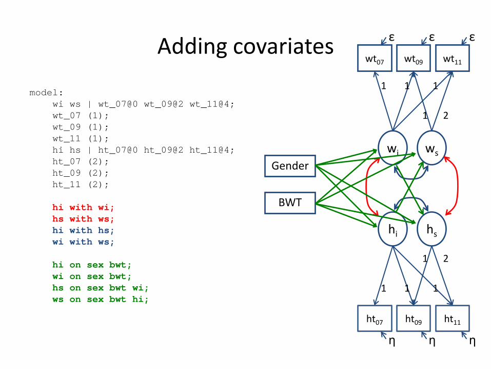
Adding covariates
model:wi ws | wt_07@0 wt_09@2 wt_11@4;wt_07 (1);wt_09 (1);wt_11 (1);hi hs | ht_07@0 ht_09@2 ht_11@4;ht_07 (2);ht_09 (2);ht_11 (2);
hi with wi;hs with ws;hi with hs;wi with ws;
hi on sex bwt;wi on sex bwt;hs on sex bwt wi;ws on sex bwt hi;
wt11wt09wt07
ε ε ε
1 1 1
1 2
wi ws
ht11ht09ht07
η η η
1 1 1
1 2
hi hs
Gender
BWT
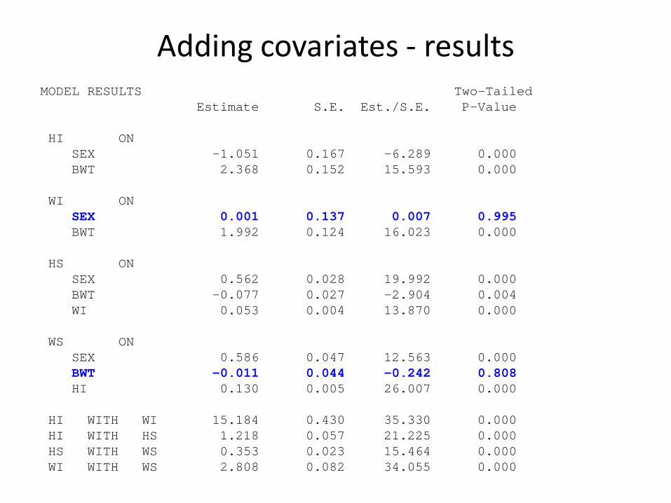
Adding covariates - resultsMODEL RESULTS Two-Tailed
Estimate S.E. Est./S.E. P-Value
HI ONSEX -1.051 0.167 -6.289 0.000BWT 2.368 0.152 15.593 0.000
WI ONSEX 0.001 0.137 0.007 0.995BWT 1.992 0.124 16.023 0.000
HS ONSEX 0.562 0.028 19.992 0.000BWT -0.077 0.027 -2.904 0.004WI 0.053 0.004 13.870 0.000
WS ONSEX 0.586 0.047 12.563 0.000BWT -0.011 0.044 -0.242 0.808HI 0.130 0.005 26.007 0.000
HI WITH WI 15.184 0.430 35.330 0.000HI WITH HS 1.218 0.057 21.225 0.000HS WITH WS 0.353 0.023 15.464 0.000WI WITH WS 2.808 0.082 34.055 0.000