tidal interaction in compact binaries: a post-newtonian ... · tidal interaction in compact...
TRANSCRIPT

Parma Workshop on Numerical Relativity and Gravitational Waves Parma, 7/9 - 9/9 2011
Tidal interaction in compact binaries: a post-Newtonian affine framework
Leonardo Gualtieri
Sapienza Università di Roma
Based on: V. Ferrari, L. G., A. Maselli, in preparation

Parma Workshop on Numerical Relativity and Gravitational Waves Parma, 7/9 - 9/9 2011
BH-NS & NS-NS coalescing binariesare among the most promising sources for GW interferometers.
They are also interesting objects on their own:for instance, are possible engine for short GRB.
Therefore, a great effort has been made to model these processes,
in order to understand their behaviourand predict the emitted gravitational waveforms.
Remark: unlike BH-BH binary coalescences, this process depends (and gives information on) both
General Relativity and the stellar fluid (tidal deformation, EOS, etc.).Many ingredients can make the physics much more complicate
than in pure BH spacetimes.

Parma Workshop on Numerical Relativity and Gravitational Waves Parma, 7/9 - 9/9 2011
How to model BH-NS & NS-NS binary coalescences?
1) Numerical Relativity
Integrations of fully non-linear Einstein’s equations are the only approach which can describe
the last phase of the inspiral, when stellar disruption occurs, and the merger.
However:
- Heavy computational cost reduces the accessible parameter space
- It may be difficult to prepare truly general initial data (i.e. non- aligned spins), and they can introduce spurious numerical effects, like non-physical eccentricity
- Generally, NR is more succesful when it can rely on some knowledge by analytical or semi-analytical approaches on the process undes study

Parma Workshop on Numerical Relativity and Gravitational Waves Parma, 7/9 - 9/9 2011
2) Post-Newtonian methods
Very accurate description of the inspiral phase,when objects are treated as pointlike.
EOB approaches (see Nagar talk), through appropriate fine-tuned parameters
whose values are inferred by NR simulations,seem to provide waveforms extending through the merger process.
Can be very useful to find large sets of GW templateswithout too much computational cost
(if it works well in the entire parameter space).However, if one wants to have a complete picture of the process,to have deeper physical insight (which may be useful to help NR),
other approaches should be pursued as well.
Parma Workshop on Numerical Relativity and Gravitational Waves Parma, 7/9 - 9/9 2011
2) Post-Newtonian methods
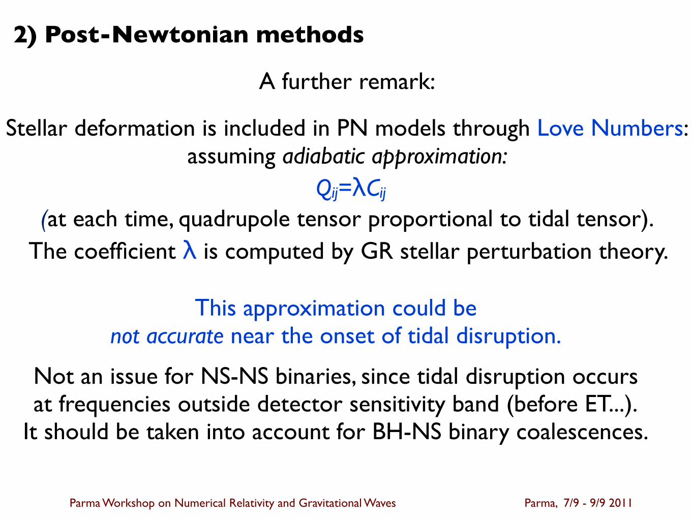
Stellar deformation is included in PN models through Love Numbers:assuming adiabatic approximation:
Qij=λCij
(at each time, quadrupole tensor proportional to tidal tensor).The coefficient λ is computed by GR stellar perturbation theory.
This approximation could be not accurate near the onset of tidal disruption.
Not an issue for NS-NS binaries, since tidal disruption occursat frequencies outside detector sensitivity band (before ET...).
It should be taken into account for BH-NS binary coalescences.
A further remark:

Parma Workshop on Numerical Relativity and Gravitational Waves Parma, 7/9 - 9/9 2011
3) Affine approaches
Introduced by Carter and Luminet in the ‘80s.The star is described as a deformable ellipsoid,
subjected to its self-gravity, internal pressure forcesand the tidal field of the companion.
- In the original formulation: Newtonian NS structure, polytropic EOS (Carter, Luminet, Marck ’85; Wiggins, Lai ’00)
- Improved formulation: GR self-gravity potential, general EOS (Ferrari, Gualtieri, Pannarale ’09,’10; Pannarale, Tonita, Rezzolla ’11).
Fluid motion (in the cdm frame) encoded in the five variables[ai(t),φ(t),λ(t)]
solution of a simple ODE system.

Parma Workshop on Numerical Relativity and Gravitational Waves Parma, 7/9 - 9/9 2011
3) Affine approaches
Some limits and approximations of this approach:
- Tidal field derived assuming that the NS moves in a geodesic of the gravitational field generated by the companion alone (Schwarzschild/Kerr). Crude approximation unless q=m1m2<<1. This can overestimate the deformation: computing tidal tensor of a Kerr BH and assuming circular orbit, divergence at light ring (i.e. breakup of the approximation) which affects also larger r
- In some formulations, orbital motion in one-body metric; in other, PN two-body orbital motion, but then mismatch in the coordinate frames (tidal field still one-body)
- Time-dilation factors neglected (relevant near the ISCO)
- Most works quasi-stationary: dynamical equations not evolved- Internal dynamics: Newtonian + GR corrections
Parma Workshop on Numerical Relativity and Gravitational Waves Parma, 7/9 - 9/9 2011
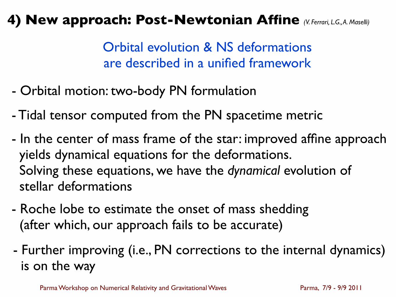
4) New approach: Post-Newtonian Affine (V. Ferrari, L.G., A. Maselli)
Orbital evolution & NS deformationsare described in a unified framework
- Orbital motion: two-body PN formulation
- Tidal tensor computed from the PN spacetime metric
- In the center of mass frame of the star: improved affine approach yields dynamical equations for the deformations. Solving these equations, we have the dynamical evolution of stellar deformations
- Roche lobe to estimate the onset of mass shedding (after which, our approach fails to be accurate)
- Further improving (i.e., PN corrections to the internal dynamics) is on the way

Parma Workshop on Numerical Relativity and Gravitational Waves Parma, 7/9 - 9/9 2011
New approach: Post-Newtonian Affine
Orbital motion: 3PN
3
A. The a!ne model
The basic assumption in the a!ne model is that theNS, deformed by the tidal field of the companion, pre-serves an ellipsoidal shape; it is an S-type Riemann el-lipsoid [33], i.e., its spin and its vorticity are parallel andtheir ratio is constant. The equilibrium structure of theNS is determined using the equations of General Rela-tivity and its dynamical behaviour is governed by New-tonian hydrodynamics improved by the use of an e"ec-tive relativistic potential. The deformation equations arewritten in the principal frame, i.e., the frame comovingwith the star whose axes are the principal axes of the el-lipsoid; in our conventions, ’1’ denotes the direction alongthe axis directed towards the companion, ’2’ is the direc-tion along the other axis that lies in the orbital plane and’3’ is associated with the direction of the axis orthogonalto the orbital plane. Surfaces of constant density insidethe star form self-similar ellipsoids and the velocity of afluid element is a linear function of the coordinates xi inthe principal frame. Under these assumptions, we canreduce the infinite degrees of freedom of the stellar fluidto five dynamic variables and work with a set of di"eren-tial equations describing the evolution of the star. Thefive variables describing the stellar deformation are thethree principal axes of the ellipsoid ai (i = 1, 2, 3) andtwo angles !, " defined as
d!
d#= # ,
d"
d#= $ , (4)
where # is the NS proper time and # the ellipsoid an-gular velocity mesured in the parallel transported frameassociated with the star center of mass. $, associated tothe internal fluid motion, is defined as follows:
$ =a1a2
a21 + a22$ , (5)
with $ vorticity along the z!axis in the corotating frame.Following [15, 17], we describe the NS internal dynamics
in terms of the Lagrangian
LI = TI ! U ! V (6)
where TI is the kinetic energy of the star interior, U isthe internal energy of the stellar fluid and V is the starself-gravity. From [13, 33] we have
TI =!
i
1
2
"aiai
#2 $d3x%x3
i +1
2
%"a1a2
$! #
#2
"
"$
d3x%x22 +
"#! a2
a1$
#2 $d3x%x2
1
&(7)
dU =!
i
%
aidai (8)
V =1
2V RNS
$ !
0
d&'(a21 + &)(a22 + &)(a23 + &)
, (9)
where RNS is the neutron star radius, % is the pressureintegral [13], and V is the self-gravity potential, given by[17]
(V = !4'
$ RNS
0
d&TOV
drr3%dr . (10)
Here d&TOV /dr is given by the Tolman-Oppenheimer-Volko" (TOV) stellar structure equations (in G = c = 1units)
d&TOV
dr=
[((r) + P (r)][mTOV (r) + 4'r3P (r)]
%(r)r[r ! 2mTOV (r)]
mTOV (r) = 4'
$ r
0dr"r"2((r") .
We assume that the NS is non-rotating in its locally in-ertial, parallel transported frame, i.e., that the fluid isirrotational. However, our approach can easily be gener-alized to rotating NSs.
B. Post-Newtonian framework
The starting point of our computation is the the3PN metric written in harmonic coordinates ({x0 =ct, x, y, z}):
g00 = !1 +2V
c2! 2V 2
c4+
8
c6
)X ++ViVi +
V
6
*+
32
c8
%T ! V X
2+ RiVi !
V ViVi
2! V 4
48
&+O(10) (11)
g0i = ! 4
c3Vi !
8
c5Ri !
16
c7
)Yi +
1
2WijVj +
1
2V 2Vi
*+O(9) (12)
gij = )ij
)1 +
2
c2V +
2
c4V 2 +
8
c6
"X + VkVk +
V 3
6
#*+
4
c4Wij +
16
c6
"Zij +
1
2V Wij ! ViVj
#+O(6) , (13)
where the potentials V, Vi, X, Wij , Ri,Yi,Zij , are definedin terms of retarded integrals over the source densities
[34, 35]. Since these potentials are written as expansion
4
of powers of 1/cn, in the following we identify the orderof the expansion with a superscript. So V (0) defines thescalar potential with zero powers of 1/c, V (2) the 1/c2
terms and so on.From Eqns. (11)-(13), we derive both the equations
describing the orbital motion of the compact binary, andthe tidal tensor which induces the deformation of the NSof mass m1.
C. The orbital motion
As discussed in the Introduction, in this paper we arenot studying the e!ects of tidal deformation on the or-bital motion. Therefore, we model the orbital motiontreating the bodies as pointlike, using the PN approachup to 3 PN order. Following [39], we assume an adia-batic inspiral of quasi-circular orbits, i.e. such that theenergy carried out by GWs is balanced by the change ofthe total binding energy of the system
dE
dt= !L . (14)
More precisaly, we employ expressions for the GW fluxL and the binding energy E up to 3 PN order, includ-ing spin e!ects (see Appendix A). We remark that weconsider the PN order with respect to the leading term,both in the binding energy and in the flux; this way ofcounting has been recognized to be the most appropriateto model of the orbital motion [40]. These quantities areexpressed in terms of the variable
x =
!Gm!
c3
"2/3
. (15)
Eq. (14) allows to compute the orbital phase "(t) andthe the orbital frequency " = ". We remark that weare neglecting orbital eccentricity; indeed, gravitationalwaves (GWs) emission causes the orbit of a binary sys-tem to circularize [36] well before the latest stages of theinspiral, which we are studying.We employ the Taylor T1 approximant, which consists
in numerically solving the ODEs
dx
dt= ! L
dE/dx(16)
d"
dt=
c3
Gmx3/2 . (17)
Since, as we shall discuss in the next Section, we alsoneed the radial coordinate r(t) and r(t), we employ thePN expression for # = Gm
rc2 , which is also known up to 3PN order including spin terms [41], and yields
# =dx
dt
#1 + 2x
$1! $
3
%+
5
2x3/2
!5
3s! + %&!
"+
+ 3x2
!1! 65
12$
"+
7
2x5/2
&!10
3+
8
9$
"s!+
+ 2%&! ] + 4x3
&1 +
!!2203
2520! 41
192'2
"$+
+229
36$2 +
$2
81
'(, (18)
where % = m1!m2m and the spin variables are defined as
follows
s! =S
Gm2=
S1 + S2
Gm2(19)
&! =!
Gm2=
1
Gm
&S2
m2! S1
m1
'; (20)
Si = m2i aisi are the spin angular momenta for bodies
i = 1, 2, with dimensionless spin parameters ai and unitdirection vectors si.We finally remark that it has been estimated [23] that,
in NS-NS inspirals, the error which is done neglectingtidal e!ects in the orbital motion, is comparable withthe error due to employing PN expressions at order 3PN instead of 3.5 PN, and it is also comparable withthe discrepancy between di!erent PN approximant (i.e.,using T4 approximants instead of T1 approximants). Wedo not expect that this picture radically changes for NS-BH inspirals. In this article, we are not addressing thelevel of accuracy at which all these e!ects show up.
D. Post-Newtonian tidal deformation
Tidal deformation in general relativity has been stud-ied by many authors (see for instance [45, 46]). The basicequation to describe tidal interaction is the geodesic de-viation equation:
d2("
d)2+R"
#$%u#u$(% = 0 (21)
where u# is the 4!velocity of a point O" (in our case,the center of the star), (" the 4!separation vector be-tween O" and another point (in our case, a generic fluidelement), and R"
#$% the Riemann tensor. It’s possible toshow that this equation can be cast in the form [47]
d2(i
d)2+ Ci
j(j = 0 , (22)
by introducing an orthonormal tetrad field e(i) (i =0, . . . , 3) associated with the frame centered in O" andparallel transported along its motion, and such that
eµ(0) = uµ. The (i = e(i)µ (µ are the tetrad components
of the displacement vector, and Cij are the component
of the relativistic tidal tensor, defined as (1):
Cij = R"#$%e"(0)e
#(i)e
µ(0)e
&(j) . (23)
Eq. (22) applies to our model with ((i) = ai.In the following sections we determine, starting from
the 3PN metric Eq.(11)-(13), the parallel transportedtetrad, the components of R"#$% and finally the tidaltensor.
=>
4
of powers of 1/cn, in the following we identify the orderof the expansion with a superscript. So V (0) defines thescalar potential with zero powers of 1/c, V (2) the 1/c2
terms and so on.From Eqns. (11)-(13), we derive both the equations
describing the orbital motion of the compact binary, andthe tidal tensor which induces the deformation of the NSof mass m1.
C. The orbital motion
As discussed in the Introduction, in this paper we arenot studying the e!ects of tidal deformation on the or-bital motion. Therefore, we model the orbital motiontreating the bodies as pointlike, using the PN approachup to 3 PN order. Following [39], we assume an adia-batic inspiral of quasi-circular orbits, i.e. such that theenergy carried out by GWs is balanced by the change ofthe total binding energy of the system
dE
dt= !L . (14)
More precisaly, we employ expressions for the GW fluxL and the binding energy E up to 3 PN order, includ-ing spin e!ects (see Appendix A). We remark that weconsider the PN order with respect to the leading term,both in the binding energy and in the flux; this way ofcounting has been recognized to be the most appropriateto model of the orbital motion [40]. These quantities areexpressed in terms of the variable
x =
!Gm!
c3
"2/3
. (15)
Eq. (14) allows to compute the orbital phase "(t) andthe the orbital frequency " = ". We remark that weare neglecting orbital eccentricity; indeed, gravitationalwaves (GWs) emission causes the orbit of a binary sys-tem to circularize [36] well before the latest stages of theinspiral, which we are studying.We employ the Taylor T1 approximant, which consists
in numerically solving the ODEs
dx
dt= ! L
dE/dx(16)
d"
dt=
c3
Gmx3/2 . (17)
Since, as we shall discuss in the next Section, we alsoneed the radial coordinate r(t) and r(t), we employ thePN expression for # = Gm
rc2 , which is also known up to 3PN order including spin terms [41], and yields
# =dx
dt
#1 + 2x
$1! $
3
%+
5
2x3/2
!5
3s! + %&!
"+
+ 3x2
!1! 65
12$
"+
7
2x5/2
&!10
3+
8
9$
"s!+
+ 2%&! ] + 4x3
&1 +
!!2203
2520! 41
192'2
"$+
+229
36$2 +
$2
81
'(, (18)
where % = m1!m2m and the spin variables are defined as
follows
s! =S
Gm2=
S1 + S2
Gm2(19)
&! =!
Gm2=
1
Gm
&S2
m2! S1
m1
'; (20)
Si = m2i aisi are the spin angular momenta for bodies
i = 1, 2, with dimensionless spin parameters ai and unitdirection vectors si.We finally remark that it has been estimated [23] that,
in NS-NS inspirals, the error which is done neglectingtidal e!ects in the orbital motion, is comparable withthe error due to employing PN expressions at order 3PN instead of 3.5 PN, and it is also comparable withthe discrepancy between di!erent PN approximant (i.e.,using T4 approximants instead of T1 approximants). Wedo not expect that this picture radically changes for NS-BH inspirals. In this article, we are not addressing thelevel of accuracy at which all these e!ects show up.
D. Post-Newtonian tidal deformation
Tidal deformation in general relativity has been stud-ied by many authors (see for instance [45, 46]). The basicequation to describe tidal interaction is the geodesic de-viation equation:
d2("
d)2+R"
#$%u#u$(% = 0 (21)
where u# is the 4!velocity of a point O" (in our case,the center of the star), (" the 4!separation vector be-tween O" and another point (in our case, a generic fluidelement), and R"
#$% the Riemann tensor. It’s possible toshow that this equation can be cast in the form [47]
d2(i
d)2+ Ci
j(j = 0 , (22)
by introducing an orthonormal tetrad field e(i) (i =0, . . . , 3) associated with the frame centered in O" andparallel transported along its motion, and such that
eµ(0) = uµ. The (i = e(i)µ (µ are the tetrad components
of the displacement vector, and Cij are the component
of the relativistic tidal tensor, defined as (1):
Cij = R"#$%e"(0)e
#(i)e
µ(0)e
&(j) . (23)
Eq. (22) applies to our model with ((i) = ai.In the following sections we determine, starting from
the 3PN metric Eq.(11)-(13), the parallel transportedtetrad, the components of R"#$% and finally the tidaltensor.
Radial motion from
10
IV. CONCLUDING REMARKS
ACKNOWLEDGEMENTS
We thank F. Pannarale and L. Rezzolla for useful dis-cussions. We thank Z. Etienne, K. Kyutoku, F. Pannar-ale and their groups for giving us the results of their fullynumerical simulations, to compare with our model. Thiswork was partially supported by CompStar, a researchnetworking program of the European Science Founda-tion. L.G. has been partially supported by Grant No.PTDC/FIS/098025/2008.
Appendix A: Post-Newtonian expressions for theorbital motion
In this Appendix we write explicitly the Post-Newtonian binding energy and the gravitational lumi-nosity up to the 3PN order for spinning bodies in quasi-circular orbits, with spins aligned with the direction ofthe Newtonian orbital angular momentum vector [39]:
E = !1
2m ! c2 x
!1 + x
"!3
4! !
12
#+ x3/2
"143s! + 2"#!
#
+x2"!27
8+
19
8! ! !2
24
#+ x5/2
"11s! + 3"#!
+!$!61
9s! !
10
3"#!
%#+ x3
"!675
64+
&34445
576! 205
96$2
'!
!155
96!2 ! 35
5184!3#(
. (A1)
and
F =32
5
c5
Gx5 !2
!1 + x
"!1247
336! 35
12!#
+x3/2"4$ ! 4s! !
5
4"#!
#+ x2
"!44711
9072+
9271
504! +
65
18!2
#
+x5/2"!8191
672$ ! 9
2s! !
13
16"#! + !
$!583
24$ +
272
9s! +
43
4"#!
%#
+x3"6643739519
69854400+
16
3$2 ! 1712
105%E ! 856
105ln(16 x)! 16$s!
!31$
6"#! + !
$!134543
7776+
41
48$2
%! 94403
3024!2 ! 775
324!3
#(.
(A2)
with %E is the Euler constant and the spin variables arethe same defined in section A.
Appendix B: The tidal tensor
We show the non vanishing components of the tidaltensor Ci
j up to the 1/c3 order, as function of the PNpotentials:
Cxx = !&2xxV
(0) +1
c2
)! 4&2
xtV(0)x + 4vy&
2xxV
(0)y ! 4vy&
2xyV
(0)x ! (&yV
(0))2 ! &2xxV
(2) !&&2tt + v2y(&
2yy + 2&2
xx) +
+ 2vy&2yt ! (2Qxy + vxvy) &
2xy
'V (0) + 2&2
xxV(0)V (0) + 2(&xV
(0))2*
! 4
c3
+(&2
xt + vy&2xy)V
(1)x ! vy&
2xxV
(1)y
,,(B1)
Cyy = !&2yyV
(0) +1
c2
)! 4&2
ytV(0)y ! (&xV
(0))2 + 4vx&2yyV
(0)x ! 4vx&
2xyV
(0)y ! &2
yyV(2) !
&&2tt + v2x(&
2xx + 2&2
yy) +
+ 2vx&2xt ! (2Qyx + vxvy) &
2xy
'V (0) + 2&2
yyV(0)V (0) + 2(&yV
(0))2*
! 4
c3
+(&2
yt + vx&2xy)V
(1)y ! vx&
2yyV
(1)x
,,(B2)
Czz = !&2zzV
(0) +1
c2
)4vy&
2zzV
(0)y + 4vx&
2zzV
(0)x ! &2
zzV(2) ! (&xV
(0))2 ! (&yV(0))2 !
&&2tt + 2
-v2x + v2y
.&2zz +
+ 2vx&2xt + 2vy&
2yt + v2x&
2xx + v2y&
2yy + 2vxvy&
2xy
'V (0) + 2&2
zzV(0)V (0)
*+
4
c3
+vy&
2zzV
(1)y + vx&
2zzV
(1)x
,, (B3)
Cxy = !&2xyV
(0) +1
c2
)&vy&
2xt + vx&
2yt +
3
2vxvy(&
2xx + &2
yy) +Qxy(&2yy ! &2
xx)!/v2x + v2y
2
0&2xy
'V (0) +
+ 3&xV(0)&yV
(0) ! &2xyV
(2) + 2&2xyV
(0)V (0) + 2(vx&2xy ! vy&
2yy ! &2
yt)V(0)x + 2(vy&
2xy ! vx&
2xx ! &2
xt)V(0)y
*
+2
c3
+(vx&
2xy ! vy&
2yy ! &2
yt)V(1)x + (vy&
2xy ! vx&
2xx ! &2
xt)V(1)y
,. (B4)
10
IV. CONCLUDING REMARKS
ACKNOWLEDGEMENTS
We thank F. Pannarale and L. Rezzolla for useful dis-cussions. We thank Z. Etienne, K. Kyutoku, F. Pannar-ale and their groups for giving us the results of their fullynumerical simulations, to compare with our model. Thiswork was partially supported by CompStar, a researchnetworking program of the European Science Founda-tion. L.G. has been partially supported by Grant No.PTDC/FIS/098025/2008.
Appendix A: Post-Newtonian expressions for theorbital motion
In this Appendix we write explicitly the Post-Newtonian binding energy and the gravitational lumi-nosity up to the 3PN order for spinning bodies in quasi-circular orbits, with spins aligned with the direction ofthe Newtonian orbital angular momentum vector [39]:
E = !1
2m ! c2 x
!1 + x
"!3
4! !
12
#+ x3/2
"143s! + 2"#!
#
+x2"!27
8+
19
8! ! !2
24
#+ x5/2
"11s! + 3"#!
+!$!61
9s! !
10
3"#!
%#+ x3
"!675
64+
&34445
576! 205
96$2
'!
!155
96!2 ! 35
5184!3#(
. (A1)
and
F =32
5
c5
Gx5 !2
!1 + x
"!1247
336! 35
12!#
+x3/2"4$ ! 4s! !
5
4"#!
#+ x2
"!44711
9072+
9271
504! +
65
18!2
#
+x5/2"!8191
672$ ! 9
2s! !
13
16"#! + !
$!583
24$ +
272
9s! +
43
4"#!
%#
+x3"6643739519
69854400+
16
3$2 ! 1712
105%E ! 856
105ln(16 x)! 16$s!
!31$
6"#! + !
$!134543
7776+
41
48$2
%! 94403
3024!2 ! 775
324!3
#(.
(A2)
with %E is the Euler constant and the spin variables arethe same defined in section A.
Appendix B: The tidal tensor
We show the non vanishing components of the tidaltensor Ci
j up to the 1/c3 order, as function of the PNpotentials:
Cxx = !&2xxV
(0) +1
c2
)! 4&2
xtV(0)x + 4vy&
2xxV
(0)y ! 4vy&
2xyV
(0)x ! (&yV
(0))2 ! &2xxV
(2) !&&2tt + v2y(&
2yy + 2&2
xx) +
+ 2vy&2yt ! (2Qxy + vxvy) &
2xy
'V (0) + 2&2
xxV(0)V (0) + 2(&xV
(0))2*
! 4
c3
+(&2
xt + vy&2xy)V
(1)x ! vy&
2xxV
(1)y
,,(B1)
Cyy = !&2yyV
(0) +1
c2
)! 4&2
ytV(0)y ! (&xV
(0))2 + 4vx&2yyV
(0)x ! 4vx&
2xyV
(0)y ! &2
yyV(2) !
&&2tt + v2x(&
2xx + 2&2
yy) +
+ 2vx&2xt ! (2Qyx + vxvy) &
2xy
'V (0) + 2&2
yyV(0)V (0) + 2(&yV
(0))2*
! 4
c3
+(&2
yt + vx&2xy)V
(1)y ! vx&
2yyV
(1)x
,,(B2)
Czz = !&2zzV
(0) +1
c2
)4vy&
2zzV
(0)y + 4vx&
2zzV
(0)x ! &2
zzV(2) ! (&xV
(0))2 ! (&yV(0))2 !
&&2tt + 2
-v2x + v2y
.&2zz +
+ 2vx&2xt + 2vy&
2yt + v2x&
2xx + v2y&
2yy + 2vxvy&
2xy
'V (0) + 2&2
zzV(0)V (0)
*+
4
c3
+vy&
2zzV
(1)y + vx&
2zzV
(1)x
,, (B3)
Cxy = !&2xyV
(0) +1
c2
)&vy&
2xt + vx&
2yt +
3
2vxvy(&
2xx + &2
yy) +Qxy(&2yy ! &2
xx)!/v2x + v2y
2
0&2xy
'V (0) +
+ 3&xV(0)&yV
(0) ! &2xyV
(2) + 2&2xyV
(0)V (0) + 2(vx&2xy ! vy&
2yy ! &2
yt)V(0)x + 2(vy&
2xy ! vx&
2xx ! &2
xt)V(0)y
*
+2
c3
+(vx&
2xy ! vy&
2yy ! &2
yt)V(1)x + (vy&
2xy ! vx&
2xx ! &2
xt)V(1)y
,. (B4)
4
of powers of 1/cn, in the following we identify the orderof the expansion with a superscript. So V (0) defines thescalar potential with zero powers of 1/c, V (2) the 1/c2
terms and so on.From Eqns. (11)-(13), we derive both the equations
describing the orbital motion of the compact binary, andthe tidal tensor which induces the deformation of the NSof mass m1.
C. The orbital motion
As discussed in the Introduction, in this paper we arenot studying the e!ects of tidal deformation on the or-bital motion. Therefore, we model the orbital motiontreating the bodies as pointlike, using the PN approachup to 3 PN order. Following [39], we assume an adia-batic inspiral of quasi-circular orbits, i.e. such that theenergy carried out by GWs is balanced by the change ofthe total binding energy of the system
dE
dt= !L . (14)
More precisaly, we employ expressions for the GW fluxL and the binding energy E up to 3 PN order, includ-ing spin e!ects (see Appendix A). We remark that weconsider the PN order with respect to the leading term,both in the binding energy and in the flux; this way ofcounting has been recognized to be the most appropriateto model of the orbital motion [40]. These quantities areexpressed in terms of the variable
x =
!Gm!
c3
"2/3
. (15)
Eq. (14) allows to compute the orbital phase "(t) andthe the orbital frequency " = ". We remark that weare neglecting orbital eccentricity; indeed, gravitationalwaves (GWs) emission causes the orbit of a binary sys-tem to circularize [36] well before the latest stages of theinspiral, which we are studying.We employ the Taylor T1 approximant, which consists
in numerically solving the ODEs
dx
dt= ! L
dE/dx(16)
d"
dt=
c3
Gmx3/2 . (17)
Since, as we shall discuss in the next Section, we alsoneed the radial coordinate r(t) and r(t), we employ thePN expression for # = Gm
rc2 , which is also known up to 3PN order including spin terms [41], and yields
# =dx
dt
#1 + 2x
$1! $
3
%+
5
2x3/2
!5
3s! + %&!
"+
+ 3x2
!1! 65
12$
"+
7
2x5/2
&!10
3+
8
9$
"s!+
+ 2%&! ] + 4x3
&1 +
!!2203
2520! 41
192'2
"$+
+229
36$2 +
$2
81
'(, (18)
where % = m1!m2m and the spin variables are defined as
follows
s! =S
Gm2=
S1 + S2
Gm2(19)
&! =!
Gm2=
1
Gm
&S2
m2! S1
m1
'; (20)
Si = m2i aisi are the spin angular momenta for bodies
i = 1, 2, with dimensionless spin parameters ai and unitdirection vectors si.We finally remark that it has been estimated [23] that,
in NS-NS inspirals, the error which is done neglectingtidal e!ects in the orbital motion, is comparable withthe error due to employing PN expressions at order 3PN instead of 3.5 PN, and it is also comparable withthe discrepancy between di!erent PN approximant (i.e.,using T4 approximants instead of T1 approximants). Wedo not expect that this picture radically changes for NS-BH inspirals. In this article, we are not addressing thelevel of accuracy at which all these e!ects show up.
D. Post-Newtonian tidal deformation
Tidal deformation in general relativity has been stud-ied by many authors (see for instance [45, 46]). The basicequation to describe tidal interaction is the geodesic de-viation equation:
d2("
d)2+R"
#$%u#u$(% = 0 (21)
where u# is the 4!velocity of a point O" (in our case,the center of the star), (" the 4!separation vector be-tween O" and another point (in our case, a generic fluidelement), and R"
#$% the Riemann tensor. It’s possible toshow that this equation can be cast in the form [47]
d2(i
d)2+ Ci
j(j = 0 , (22)
by introducing an orthonormal tetrad field e(i) (i =0, . . . , 3) associated with the frame centered in O" andparallel transported along its motion, and such that
eµ(0) = uµ. The (i = e(i)µ (µ are the tetrad components
of the displacement vector, and Cij are the component
of the relativistic tidal tensor, defined as (1):
Cij = R"#$%e"(0)e
#(i)e
µ(0)e
&(j) . (23)
Eq. (22) applies to our model with ((i) = ai.In the following sections we determine, starting from
the 3PN metric Eq.(11)-(13), the parallel transportedtetrad, the components of R"#$% and finally the tidaltensor.
and the PN expression for
4
of powers of 1/cn, in the following we identify the orderof the expansion with a superscript. So V (0) defines thescalar potential with zero powers of 1/c, V (2) the 1/c2
terms and so on.From Eqns. (11)-(13), we derive both the equations
describing the orbital motion of the compact binary, andthe tidal tensor which induces the deformation of the NSof mass m1.
C. The orbital motion
As discussed in the Introduction, in this paper we arenot studying the e!ects of tidal deformation on the or-bital motion. Therefore, we model the orbital motiontreating the bodies as pointlike, using the PN approachup to 3 PN order. Following [39], we assume an adia-batic inspiral of quasi-circular orbits, i.e. such that theenergy carried out by GWs is balanced by the change ofthe total binding energy of the system
dE
dt= !L . (14)
More precisaly, we employ expressions for the GW fluxL and the binding energy E up to 3 PN order, includ-ing spin e!ects (see Appendix A). We remark that weconsider the PN order with respect to the leading term,both in the binding energy and in the flux; this way ofcounting has been recognized to be the most appropriateto model of the orbital motion [40]. These quantities areexpressed in terms of the variable
x =
!Gm!
c3
"2/3
. (15)
Eq. (14) allows to compute the orbital phase "(t) andthe the orbital frequency " = ". We remark that weare neglecting orbital eccentricity; indeed, gravitationalwaves (GWs) emission causes the orbit of a binary sys-tem to circularize [36] well before the latest stages of theinspiral, which we are studying.We employ the Taylor T1 approximant, which consists
in numerically solving the ODEs
dx
dt= ! L
dE/dx(16)
d"
dt=
c3
Gmx3/2 . (17)
Since, as we shall discuss in the next Section, we alsoneed the radial coordinate r(t) and r(t), we employ thePN expression for # = Gm
rc2 , which is also known up to 3PN order including spin terms [41], and yields
# =dx
dt
#1 + 2x
$1! $
3
%+
5
2x3/2
!5
3s! + %&!
"+
+ 3x2
!1! 65
12$
"+
7
2x5/2
&!10
3+
8
9$
"s!+
+ 2%&! ] + 4x3
&1 +
!!2203
2520! 41
192'2
"$+
+229
36$2 +
$2
81
'(, (18)
where % = m1!m2m and the spin variables are defined as
follows
s! =S
Gm2=
S1 + S2
Gm2(19)
&! =!
Gm2=
1
Gm
&S2
m2! S1
m1
'; (20)
Si = m2i aisi are the spin angular momenta for bodies
i = 1, 2, with dimensionless spin parameters ai and unitdirection vectors si.We finally remark that it has been estimated [23] that,
in NS-NS inspirals, the error which is done neglectingtidal e!ects in the orbital motion, is comparable withthe error due to employing PN expressions at order 3PN instead of 3.5 PN, and it is also comparable withthe discrepancy between di!erent PN approximant (i.e.,using T4 approximants instead of T1 approximants). Wedo not expect that this picture radically changes for NS-BH inspirals. In this article, we are not addressing thelevel of accuracy at which all these e!ects show up.
D. Post-Newtonian tidal deformation
Tidal deformation in general relativity has been stud-ied by many authors (see for instance [45, 46]). The basicequation to describe tidal interaction is the geodesic de-viation equation:
d2("
d)2+R"
#$%u#u$(% = 0 (21)
where u# is the 4!velocity of a point O" (in our case,the center of the star), (" the 4!separation vector be-tween O" and another point (in our case, a generic fluidelement), and R"
#$% the Riemann tensor. It’s possible toshow that this equation can be cast in the form [47]
d2(i
d)2+ Ci
j(j = 0 , (22)
by introducing an orthonormal tetrad field e(i) (i =0, . . . , 3) associated with the frame centered in O" andparallel transported along its motion, and such that
eµ(0) = uµ. The (i = e(i)µ (µ are the tetrad components
of the displacement vector, and Cij are the component
of the relativistic tidal tensor, defined as (1):
Cij = R"#$%e"(0)e
#(i)e
µ(0)e
&(j) . (23)
Eq. (22) applies to our model with ((i) = ai.In the following sections we determine, starting from
the 3PN metric Eq.(11)-(13), the parallel transportedtetrad, the components of R"#$% and finally the tidaltensor.

Parma Workshop on Numerical Relativity and Gravitational Waves Parma, 7/9 - 9/9 2011
New approach: Post-Newtonian Affine
Tidal tensor:
4
of powers of 1/cn, in the following we identify the orderof the expansion with a superscript. So V (0) defines thescalar potential with zero powers of 1/c, V (2) the 1/c2
terms and so on.From Eqns. (11)-(13), we derive both the equations
describing the orbital motion of the compact binary, andthe tidal tensor which induces the deformation of the NSof mass m1.
C. The orbital motion
As discussed in the Introduction, in this paper we arenot studying the e!ects of tidal deformation on the or-bital motion. Therefore, we model the orbital motiontreating the bodies as pointlike, using the PN approachup to 3 PN order. Following [39], we assume an adia-batic inspiral of quasi-circular orbits, i.e. such that theenergy carried out by GWs is balanced by the change ofthe total binding energy of the system
dE
dt= !L . (14)
More precisaly, we employ expressions for the GW fluxL and the binding energy E up to 3 PN order, includ-ing spin e!ects (see Appendix A). We remark that weconsider the PN order with respect to the leading term,both in the binding energy and in the flux; this way ofcounting has been recognized to be the most appropriateto model of the orbital motion [40]. These quantities areexpressed in terms of the variable
x =
!Gm!
c3
"2/3
. (15)
Eq. (14) allows to compute the orbital phase "(t) andthe the orbital frequency " = ". We remark that weare neglecting orbital eccentricity; indeed, gravitationalwaves (GWs) emission causes the orbit of a binary sys-tem to circularize [36] well before the latest stages of theinspiral, which we are studying.We employ the Taylor T1 approximant, which consists
in numerically solving the ODEs
dx
dt= ! L
dE/dx(16)
d"
dt=
c3
Gmx3/2 . (17)
Since, as we shall discuss in the next Section, we alsoneed the radial coordinate r(t) and r(t), we employ thePN expression for # = Gm
rc2 , which is also known up to 3PN order including spin terms [41], and yields
# =dx
dt
#1 + 2x
$1! $
3
%+
5
2x3/2
!5
3s! + %&!
"+
+ 3x2
!1! 65
12$
"+
7
2x5/2
&!10
3+
8
9$
"s!+
+ 2%&! ] + 4x3
&1 +
!!2203
2520! 41
192'2
"$+
+229
36$2 +
$2
81
'(, (18)
where % = m1!m2m and the spin variables are defined as
follows
s! =S
Gm2=
S1 + S2
Gm2(19)
&! =!
Gm2=
1
Gm
&S2
m2! S1
m1
'; (20)
Si = m2i aisi are the spin angular momenta for bodies
i = 1, 2, with dimensionless spin parameters ai and unitdirection vectors si.We finally remark that it has been estimated [23] that,
in NS-NS inspirals, the error which is done neglectingtidal e!ects in the orbital motion, is comparable withthe error due to employing PN expressions at order 3PN instead of 3.5 PN, and it is also comparable withthe discrepancy between di!erent PN approximant (i.e.,using T4 approximants instead of T1 approximants). Wedo not expect that this picture radically changes for NS-BH inspirals. In this article, we are not addressing thelevel of accuracy at which all these e!ects show up.
D. Post-Newtonian tidal deformation
Tidal deformation in general relativity has been stud-ied by many authors (see for instance [45, 46]). The basicequation to describe tidal interaction is the geodesic de-viation equation:
d2("
d)2+R"
#$%u#u$(% = 0 (21)
where u# is the 4!velocity of a point O" (in our case,the center of the star), (" the 4!separation vector be-tween O" and another point (in our case, a generic fluidelement), and R"
#$% the Riemann tensor. It’s possible toshow that this equation can be cast in the form [47]
d2(i
d)2+ Ci
j(j = 0 , (22)
by introducing an orthonormal tetrad field e(i) (i =0, . . . , 3) associated with the frame centered in O" andparallel transported along its motion, and such that
eµ(0) = uµ. The (i = e(i)µ (µ are the tetrad components
of the displacement vector, and Cij are the component
of the relativistic tidal tensor, defined as (1):
Cij = R"#$%e"(0)e
#(i)e
µ(0)e
&(j) . (23)
Eq. (22) applies to our model with ((i) = ai.In the following sections we determine, starting from
the 3PN metric Eq.(11)-(13), the parallel transportedtetrad, the components of R"#$% and finally the tidaltensor.
- Riemann tensor in the PN metric (not available in the literature; derivatives of the PN potentials, Hadamard regularization, frame attached to the axes)
- Fermi-Walker tetrad (w.r.t. PN metric) attached to the NS
6
is the coordinate velocity, and r12 = r1 ! r2 the rela-tive displacement between the two masses. !ijk is the3!dimensional antisymmetric Levi-Civita symbol with!123 = 1 while Sj
1 is the spin-vector and contributes toour equations at 2.5 PN order only.The necessary steps in order to evaluate the tidal ten-
sor at the center of the NS (i.e., at location 1 in ourconventions) are the following:
1. estimate the variuos derivatives of the scalar andvectorial potentials V, Vi;
2. compute the tidal tensor at the source location[Ci
j ]1, and apply a regularization procedure;
3. express all quantities in the center of mass frame;
4. switch to the principal frame, i.e. the frame fixedwith the ellipsoid axes.
The second point requires further clarification. ThePN potentials show a divergence when computed at thesource location, due to the unphysical approximation ofthe source as a point particle. Therefore, we have to re-move this divergence, apply a regularization procedure,like the Hadamard regularization [34], which we herebriefly describe. Let F (x,y1,y2) be a function depend-ing on the field point x, as well as on two source pointsy1,y2, and having as x " y1 an expression of the type
F (x,y1,y2) =0!
k=!k0
rk1fk(n1,y1,y2) +O(r1) k # Z .
(37)We define the regularized value of F at the point 1 as theHadamard part finie, which is an average, with respectto the direction n1, of the term with zero powers of r1 in
the sum (37):
(F )1 = F (y1,y1,y2) =
"d!(n1)
4"f0(n1,y1,y2) . (38)
We use this procedure in order to evaluate (V )1, (Vi)1and their relative derivatives at the source point.We change coordinates to the center of mass frame,
linking the individual coordinate yi1,2 with the relativeones xi, by means of the following coordinate transfor-mation [49]
yi1 =
#m2
m+ #
m1 !m2
mP$xi +O(4) , (39)
yi2 =
#!m1
m+ #
m1 !m2
mP$xi +O(4) (40)
where
P =1
c2
#v2
2! Gm
2r
$+O(4) . (41)
Finally, we express Cij in the principal frame using the
rotation matrix
T =
%
&cos$ sin$ 0! sin$ cos$ 0
0 0 1
'
( (42)
where $ is defined by Eq.(4)
d$
d%= ! (43)
The complete form of the tidal tensor c = TCT T is givenby:
cxx = !Gm2
2r3{1 + 3 cos[2!l]}+
G4c2r4
!"6Gm2
2 + 5Gmµ+ 3r2m1"r#(1 + 3 cos[2!l]) ! 6#2m2r
3(1 + cos[2!l]) +
! 6m2r
$2Qxy !
%m2
2
m2+ 2"
&#rr
'sin[2!l]
(+
3GSz2
mc3r3
!#m2 + (m2 ! 2m1)# cos[2!l] + r
(m2 + 3m1)r
sin[2!l]
((44)
cyy = !Gm2
2r3{1! 3 cos[2!l]}+
G4c2r4
!"6Gm2
2 + 5Gmµ+ 3r2m1"r#(1! 3 cos[2!l]) ! 6#2m2r
3(1! cos[2!l]) +
+ 6m2r
$2Qxy !
%m2
2
m2+ 2"
&#rr
'sin[2!l]
(+
3Sz2
mc3r3
!#m2 ! #(m2 ! 2m1) cos[2!l]! r
(m2 + 3m1)r
sin[2!l]
((45)
czz =Gm2
r3! G
c2
)3Gm2
2
r4+
52Gmµr4
+32m1" r
2
r3! 3
rm2#
2
*! 6Gm2S
z2
mc3r3# (46)
cxy =3Gm2
2r3sin[2!l] +
3G4c2r4
!2m2r
)%m2
2
m2+ 2"
&#rr ! 2Qxy
*cos[2!l]!
+6Gm2
2 + 5Gmµ+ 3r2m1"r ! 2#2m2r3,
"
...other components...
Result:

Parma Workshop on Numerical Relativity and Gravitational Waves Parma, 7/9 - 9/9 2011
Tidal tensor:
New approach: Post-Newtonian Affine
- Computed up to 1.5PN
- Consistent with orbital motion (only one radial coordinate)
- Time dilation included
- No unphysical divergences like
- Consistent with previous computations
(Vines, Flanagan, Hinderer ’11):
7
! sin[2!l]
!" 3GSz
2
mc3r4
"r(m2 + 3m1) cos[2!l] + "(m2 " 2m1)r sin[2!l]
#(47)
where the lag angle !l = ! ! " describes the misaligne-ment between the a1 axis direction and the line betweenthe two objects. The dot superscript identifies derivativesof the orbital variables r," with respect to the coordinatetime t.
3. Comparison with previous expressions of the tidal tensor
As a first check we verify that, in the test-mass limit# " 0, the PN tidal tensor derived above coincides withthe tidal tensor derived in [46], up to the 1/c2 orderfor BH-NS binaries. For simplicity we assume that theBH is non-rotating, i.e., a = 0, and we consider the cxxcomponent (the same argument holds for the other non-vanishing terms):
cschxx =Gm2
c2R3s
!1! 3
R2s +K
R2s
cos[!l]2
", (48)
where K = L2z is the square of the orbital angular mo-
mentum along the z!direction and Rs the radial dis-tance in Scwarzschild coordinates. In order to compareEq. (48) with Eq. (44) we have to express cschxx in termsof the same radial coordinate adopted for the PN expan-sion, which, up to 2 PN order, coincides with the isotropicSchwarzschild coordinate [50]:
Rs = r
!1 +
Gm2
2c2r
"2
. (49)
We find (neglecting higher order terms in Gm22c2r )
cschxx = ! m2
2c2r3(1 + 3 cos[2!l]) +
3m2
2c4r4{m2 +
+ 3m2 cos[2!l]! "r ! "r cos[2!l]#. (50)
We see that, in the limit # " 0, neglecting all the coef-ficients multiplied by sin[2!l] in Eq.(44) (that are e!ec-tively of a higher PN order, since when both spins arezero the lag angle, i.e. the misalignent of the principalaxis with the orbital line, is only due to frame dragging),the two formultations of the tidal tensor coincide.A further clarification has to be made in order to com-
pare the PN and Schwarzschild tidal tensors. The com-ponents of cschij are derived under the assumption thatmass m1 follows a time-like geodesic of the Scwarzschildspacetime. Following [50], in this limit the constant Kcan be written for circular orbits as function of the radialdistance Rs as
K
R2s=
m2
Rs ! 3m2. (51)
The former equation shows a divegence for Rs " 3m2,that is for Rs approaching to the well known light ringorbit of the Scwarzschild space-time. The test-particleapproximation clearly fails when # = m1m2
(m1+m2)2> 0, for
which as stressed in [3] such divergence in the PN equa-tion of motion disappears. Therefore, employing the tidalfield cschij for # > 0 leads to an overestimation (which canbe significant near the innermost stable circular orbit) ofthe constant of motion K, of the tidal tensor, and thenof the tidal deformation. On the other hand, it shouldbe taken into account that for small values of # (i.e., forq # 1) our approach becomes unaccurate, since it is wellknown that the PN expansion is poorly convergent in thetest particle limit [3].As a second check we verify that our expression for
the tidal tensor corresponds to the expression employedin [27], previously derived in [28] using a completely dif-ferent approach, based on a multipole expansion ratherthan on computation of the Riemann tensor. ComparingGij
2 (Eq. (2.2) of [27]) with our tensor Cij , we find that(renaming m1 $ m2)
Cij = !Gij2 + (frame dragging terms in Qxy)
+ (spin terms O(1/c3)) . (52)
The small frame dragging terms are due a di!erent gaugechoice from [27], where the axes of the global PN frameare chosen, while in our derivation the axes are Fermi-Walker transported; the two prescriptions are almost co-incident, they only di!er due to frame dragging. Thespin terms are the 1.5 PN terms, which have not beencomputed in [27].To conclude this Section, we remark that our defini-
tion of the tidal tensor in terms of the Riemann tensoris equivalent to the definition employed by many authors(see for instance [25]) in terms of the Weyl tensor. In-deed, when we compute the tidal tensor on the body 1,we remove by Hadamard regularization the contributionof the matter located in y1; therefore, we have e!ectivelyvacuum in y1, and the Riemann and Weyl tensors docoincide in vacuum.
E. Internal dynamics
The internal dynamics of the NS is described usingan Hamiltonian approach in the a"ne approximation[13, 15], recently improved to take into account generalrelativistic e!ects [17]:
H = HT +HI (53)
where HI describes the internal structure of the NS, andHT describes the tidal interaction. We obtainHI directly

Parma Workshop on Numerical Relativity and Gravitational Waves Parma, 7/9 - 9/9 2011
New approach: Post-Newtonian Affine
Internal dynamics: the affine model
- The NS, deformed by the tidal field of the companion, preserves an ellipsoidal shape- NS equilibrium structure: GR equations (TOV)- Dynamics governed by Newtonian hydrodynamics improved by the use of an effective relativistic potential- Degrees of freedom: ai (i=1,2,3) principal axes of the ellipsoid ψ, λ angles relating the principal frame with the PN frame- Internal dynamics Lagrangian:
L = LI + LT LI = TI − U − V LT = −1
2cijIij
Tidal Tensor!

Parma Workshop on Numerical Relativity and Gravitational Waves Parma, 7/9 - 9/9 2011
New approach: Post-Newtonian Affine
TI , U , V : Newtonian integrals, improved with a relativistic effective potential ΦTOV to describe self-gravity
3
A. The a!ne model
The basic assumption in the a!ne model is that theNS, deformed by the tidal field of the companion, pre-serves an ellipsoidal shape; it is an S-type Riemann el-lipsoid [33], i.e., its spin and its vorticity are parallel andtheir ratio is constant. The equilibrium structure of theNS is determined using the equations of General Rela-tivity and its dynamical behaviour is governed by New-tonian hydrodynamics improved by the use of an e"ec-tive relativistic potential. The deformation equations arewritten in the principal frame, i.e., the frame comovingwith the star whose axes are the principal axes of the el-lipsoid; in our conventions, ’1’ denotes the direction alongthe axis directed towards the companion, ’2’ is the direc-tion along the other axis that lies in the orbital plane and’3’ is associated with the direction of the axis orthogonalto the orbital plane. Surfaces of constant density insidethe star form self-similar ellipsoids and the velocity of afluid element is a linear function of the coordinates xi inthe principal frame. Under these assumptions, we canreduce the infinite degrees of freedom of the stellar fluidto five dynamic variables and work with a set of di"eren-tial equations describing the evolution of the star. Thefive variables describing the stellar deformation are thethree principal axes of the ellipsoid ai (i = 1, 2, 3) andtwo angles !, " defined as
d!
d#= # ,
d"
d#= $ , (4)
where # is the NS proper time and # the ellipsoid an-gular velocity mesured in the parallel transported frameassociated with the star center of mass. $, associated tothe internal fluid motion, is defined as follows:
$ =a1a2
a21 + a22$ , (5)
with $ vorticity along the z!axis in the corotating frame.Following [15, 17], we describe the NS internal dynamics
in terms of the Lagrangian
LI = TI ! U ! V (6)
where TI is the kinetic energy of the star interior, U isthe internal energy of the stellar fluid and V is the starself-gravity. From [13, 33] we have
TI =!
i
1
2
"aiai
#2 $d3x%x3
i +1
2
%"a1a2
$! #
#2
"
"$
d3x%x22 +
"#! a2
a1$
#2 $d3x%x2
1
&(7)
dU =!
i
%
aidai (8)
V =1
2V RNS
$ !
0
d&'(a21 + &)(a22 + &)(a23 + &)
, (9)
where RNS is the neutron star radius, % is the pressureintegral [13], and V is the self-gravity potential, given by[17]
(V = !4'
$ RNS
0
d&TOV
drr3%dr . (10)
Here d&TOV /dr is given by the Tolman-Oppenheimer-Volko" (TOV) stellar structure equations (in G = c = 1units)
d&TOV
dr=
[((r) + P (r)][mTOV (r) + 4'r3P (r)]
%(r)r[r ! 2mTOV (r)]
mTOV (r) = 4'
$ r
0dr"r"2((r") .
We assume that the NS is non-rotating in its locally in-ertial, parallel transported frame, i.e., that the fluid isirrotational. However, our approach can easily be gener-alized to rotating NSs.
B. Post-Newtonian framework
The starting point of our computation is the the3PN metric written in harmonic coordinates ({x0 =ct, x, y, z}):
g00 = !1 +2V
c2! 2V 2
c4+
8
c6
)X ++ViVi +
V
6
*+
32
c8
%T ! V X
2+ RiVi !
V ViVi
2! V 4
48
&+O(10) (11)
g0i = ! 4
c3Vi !
8
c5Ri !
16
c7
)Yi +
1
2WijVj +
1
2V 2Vi
*+O(9) (12)
gij = )ij
)1 +
2
c2V +
2
c4V 2 +
8
c6
"X + VkVk +
V 3
6
#*+
4
c4Wij +
16
c6
"Zij +
1
2V Wij ! ViVj
#+O(6) , (13)
where the potentials V, Vi, X, Wij , Ri,Yi,Zij , are definedin terms of retarded integrals over the source densities
[34, 35]. Since these potentials are written as expansion
We are still improving this part, including PN corrections
An equation of state ρ=ρ(p) has to be be specified.
Internal dynamics: the affine model

Parma Workshop on Numerical Relativity and Gravitational Waves Parma, 7/9 - 9/9 2011
Equations of motion:
Coupled with equationsof orbital motion
(in t,r,φ).
8
from the internal Lagrangian LI (6). The tidal Hamilto-nian HT is obtained from the Lagrangian (built up withthe coe!cients cij , Eq.(44)-(46) ):
LT = !1
2cijIij , (54)
where
I = M · diag!
aiRNS
"2
is the inertia tensor of the star in the principal frame,being M and RNS the scalar quadrupole moment andthe NS radius in a spherical configuration, respectively.Indeed, it can be shown that the equations of motion forthe stellar deformation following from (54) coincide withthe tidal equation (22)
d2ai
d!2+ Ci
jaj = 0 , (55)
where dt = "d! with
"(t) = 1 +1
c2
!m2
2
m2
v2
2+
Gm2
r
"+
1
8c4r2
#4G2m2
2
! 12G2mµ+ 3m4
2
m4r2v4 + 20G
m32
m2rv2
+ 4Gm1#r(4v2 ! r2)
$. (56)
We remark that HT " !LT , since it does not depend onthe conjugate momenta.The equations of motion for the internal variables
qi = {$,%, a1, a2, a3} and their conjugate momenta pi ={p!, p", pa1 , pa2 , pa3} are:
da1dt
=RNS
"(t)
pa1
M(57)
da2dt
=RNS
"(t)
pa2
M(58)
da3dt
=RNS
"(t)
pa3
M(59)
dpa1
dt=
M"(t)
%"2 + #2 ! 2
a2a1
"#+1
2
V
MR3
NSA1
+R2
NS
M$
a21! cxx
&a1 (60)
dpa2
dt=
M"(t)
%"2 + #2 ! 2
a1a2
"#+1
2
V
MR3
NSA2
+R2
NS
M$
a22! cyy
&a2 (61)
dpa3
dt=
M"(t)
%1
2
V
MR3
NSA3 +R2
NS
M$
a23! czz
&a3 (62)
d%
dt=
"
"(t)(63)
dp"dt
=C
"(t)= 0 (64)
d$
dt=
#
"(t)(65)
dp!dt
=J1"(t)
=MRNS
cxy"(t)
'a22 ! a21
(, (66)
where J1 is the NS spin angular momentum and C is thecirculation, i.e., the conjugate momentum associated to%:
C =MR2
NS
)'a21 + a22
(" ! 2a1a2#
*.
In absence of viscosity C is a constant of motion: weset it equal to zero in order to satisfty the condition ofirrotational fluid chosen for our model.
F. Roches lobe and tidal disruption
In order to simulate a BH-NS coalescence, we evolvenumerically the equations of motion (57)-(66) up to anorbital separation rtide, at which tidal disruption sets in.In order to find the value of rtide, we estimate the Rochelobe radius of the NS during its inspiral. It defines theregion surrounding the star in which a particle of massm0 # m1 undergoes to the NS gravitational attracion.Following the strategy adopted in [51], we estimate thethree-body potential for massesm0 # m1 $ m2 (at New-tonian order) for equatorial orbits in the x! y plane:
U(x, y) = ! m1
|x! y1|! m2
|x! y2|! 1
2&2x2 (67)
where y1/2 are the m1/2 displacement vectors and thelast term is the centrifulgal contribution with
& =
+m1 +m2
r3.
Since U(x, y) takes its maximum URl on the surface defin-ing the Roche lobe, we estimate numerically U(x, y), find-ing the Roche lobe on the x!y plane. We compare thesevalues with those of the ellipsoid axes a1, a2 that are sub-ject to a deformation due to the tidal field, identifyingthe tidal disruption when either a1 or a2 is greater thanthe distance between the star center and the Roche lobesurface, along direction 1 or 2, respectively.We also determine the location of the Post-Newtonian
ICO (Innermost Circular Orbit), rICO, in order to see ifthe system reaches r = rtide in a stable orbital configura-tion. To this aim we minimize the total binding energy ofthe BH-NS system, including the spin contribution [41].If rtide > rICO, the NS is disrupted before the mergerstarts.
New approach: Post-Newtonian Affine
Internal dynamics: the affine model
8
from the internal Lagrangian LI (6). The tidal Hamilto-nian HT is obtained from the Lagrangian (built up withthe coe!cients cij , Eq.(44)-(46) ):
LT = !1
2cijIij , (54)
where
I = M · diag!
aiRNS
"2
is the inertia tensor of the star in the principal frame,being M and RNS the scalar quadrupole moment andthe NS radius in a spherical configuration, respectively.Indeed, it can be shown that the equations of motion forthe stellar deformation following from (54) coincide withthe tidal equation (22)
d2ai
d!2+ Ci
jaj = 0 , (55)
where dt = "d! with
"(t) = 1 +1
c2
!m2
2
m2
v2
2+
Gm2
r
"+
1
8c4r2
#4G2m2
2
! 12G2mµ+ 3m4
2
m4r2v4 + 20G
m32
m2rv2
+ 4Gm1#r(4v2 ! r2)
$. (56)
We remark that HT " !LT , since it does not depend onthe conjugate momenta.The equations of motion for the internal variables
qi = {$,%, a1, a2, a3} and their conjugate momenta pi ={p!, p", pa1 , pa2 , pa3} are:
da1dt
=RNS
"(t)
pa1
M(57)
da2dt
=RNS
"(t)
pa2
M(58)
da3dt
=RNS
"(t)
pa3
M(59)
dpa1
dt=
M"(t)
%"2 + #2 ! 2
a2a1
"#+1
2
V
MR3
NSA1
+R2
NS
M$
a21! cxx
&a1 (60)
dpa2
dt=
M"(t)
%"2 + #2 ! 2
a1a2
"#+1
2
V
MR3
NSA2
+R2
NS
M$
a22! cyy
&a2 (61)
dpa3
dt=
M"(t)
%1
2
V
MR3
NSA3 +R2
NS
M$
a23! czz
&a3 (62)
d%
dt=
"
"(t)(63)
dp"dt
=C
"(t)= 0 (64)
d$
dt=
#
"(t)(65)
dp!dt
=J1"(t)
=MRNS
cxy"(t)
'a22 ! a21
(, (66)
where J1 is the NS spin angular momentum and C is thecirculation, i.e., the conjugate momentum associated to%:
C =MR2
NS
)'a21 + a22
(" ! 2a1a2#
*.
In absence of viscosity C is a constant of motion: weset it equal to zero in order to satisfty the condition ofirrotational fluid chosen for our model.
F. Roches lobe and tidal disruption
In order to simulate a BH-NS coalescence, we evolvenumerically the equations of motion (57)-(66) up to anorbital separation rtide, at which tidal disruption sets in.In order to find the value of rtide, we estimate the Rochelobe radius of the NS during its inspiral. It defines theregion surrounding the star in which a particle of massm0 # m1 undergoes to the NS gravitational attracion.Following the strategy adopted in [51], we estimate thethree-body potential for massesm0 # m1 $ m2 (at New-tonian order) for equatorial orbits in the x! y plane:
U(x, y) = ! m1
|x! y1|! m2
|x! y2|! 1
2&2x2 (67)
where y1/2 are the m1/2 displacement vectors and thelast term is the centrifulgal contribution with
& =
+m1 +m2
r3.
Since U(x, y) takes its maximum URl on the surface defin-ing the Roche lobe, we estimate numerically U(x, y), find-ing the Roche lobe on the x!y plane. We compare thesevalues with those of the ellipsoid axes a1, a2 that are sub-ject to a deformation due to the tidal field, identifyingthe tidal disruption when either a1 or a2 is greater thanthe distance between the star center and the Roche lobesurface, along direction 1 or 2, respectively.We also determine the location of the Post-Newtonian
ICO (Innermost Circular Orbit), rICO, in order to see ifthe system reaches r = rtide in a stable orbital configura-tion. To this aim we minimize the total binding energy ofthe BH-NS system, including the spin contribution [41].If rtide > rICO, the NS is disrupted before the mergerstarts.
ODE system evolved up to the onset
of tidal disruption (r=rshed)i.e. when the NS surfacetouches the Roche lobe.
Attention:this happens before
the actual tidal disruption,and before the cut-off in
the gravitational waveform!

Parma Workshop on Numerical Relativity and Gravitational Waves Parma, 7/9 - 9/9 2011
Example of axes evolution:
New approach: Post-Newtonian Affine
0.97
0.98
0.99
1
1.01
1.02
1.03
1.04
1.05
1.06
1.07
35 40 45 50 55 60 65 70 75 80r (km)
q=2 C=0.145
a1a2a3
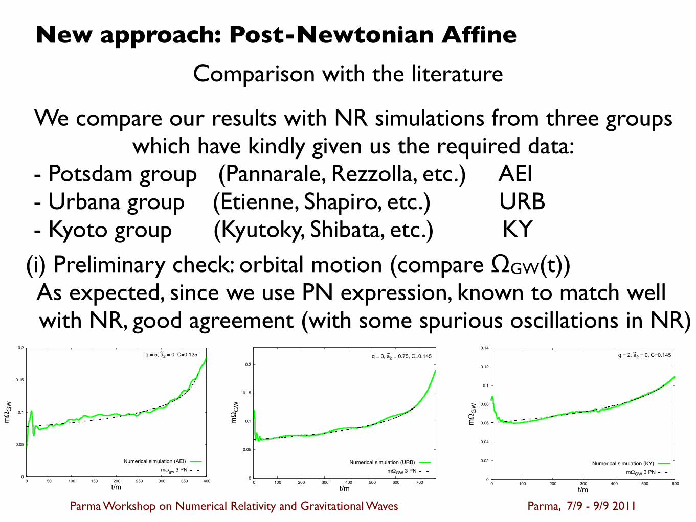
Parma Workshop on Numerical Relativity and Gravitational Waves Parma, 7/9 - 9/9 2011
New approach: Post-Newtonian Affine
Comparison with the literature
We compare our results with NR simulations from three groupswhich have kindly given us the required data:
- Potsdam group (Pannarale, Rezzolla, etc.) AEI- Urbana group (Etienne, Shapiro, etc.) URB- Kyoto group (Kyutoky, Shibata, etc.) KY
(i) Preliminary check: orbital motion (compare ΩGW(t)) As expected, since we use PN expression, known to match well with NR, good agreement (with some spurious oscillations in NR)12
0.02
0.04
0.06
0.08
0.1
0.12
0.14
0 50 100 150 200 250 300 350
mG
W
t/m
q = 5, a~2 = 0, C=0.1
Numerical simulation (AEI) m GW 3 PN
0
0.05
0.1
0.15
0.2
0 50 100 150 200 250 300 350 400
mG
W
t/m
q = 5, a~2 = 0, C=0.125
Numerical simulation (AEI) m gw 3 PN
0
0.05
0.1
0.15
0.2
0 50 100 150 200 250 300 350 400
mG
W
t/m
q = 5, a~2 = 0, C=0.145
Numerical simulation (AEI) m GW 3 PN
0
0.05
0.1
0.15
0.2
0 50 100 150 200 250 300 350
mG
W
t/m
q = 5, a~2 = 0, C=0.15
Numerical simulation (AEI) m GW 3 PN
0
0.05
0.1
0.15
0.2
0 50 100 150 200 250 300 350 400 450
mgw
t/m
q = 3, C=0.145, a~2 = 0
Numerical simulation (URB) m GW 3 PN
0
0.05
0.1
0.15
0.2
0 100 200 300 400 500 600 700
mG
W
t/m
q = 3, a~2 = 0.75, C=0.145
Numerical simulation (URB) m GW 3 PN
0
0.02
0.04
0.06
0.08
0.1
0.12
0.14
0 100 200 300 400 500 600
mG
W
t/m
q = 2, a~2 = 0, C=0.145
Numerical simulation (KY) m GW 3 PN
0
0.05
0.1
0.15
0.2
0 100 200 300 400 500
mG
W
t/m
q = 3, a~2 = 0, C=0.145
Numerical simulation (KY) m GW 3 PN
FIG. 1. (Color online) Gravitational wave frequency in thesimulations AEI, URB, KY (solid line) and in our simulations(dashed line). The dashed lines stop at r = rshed, over whichthe deformed star touch the Roche lobe.
12
0.02
0.04
0.06
0.08
0.1
0.12
0.14
0 50 100 150 200 250 300 350
mG
W
t/m
q = 5, a~2 = 0, C=0.1
Numerical simulation (AEI) m GW 3 PN
0
0.05
0.1
0.15
0.2
0 50 100 150 200 250 300 350 400
mG
W
t/m
q = 5, a~2 = 0, C=0.125
Numerical simulation (AEI) m gw 3 PN
0
0.05
0.1
0.15
0.2
0 50 100 150 200 250 300 350 400
mG
W
t/m
q = 5, a~2 = 0, C=0.145
Numerical simulation (AEI) m GW 3 PN
0
0.05
0.1
0.15
0.2
0 50 100 150 200 250 300 350
mG
W
t/m
q = 5, a~2 = 0, C=0.15
Numerical simulation (AEI) m GW 3 PN
0
0.05
0.1
0.15
0.2
0 50 100 150 200 250 300 350 400 450
mgw
t/m
q = 3, C=0.145, a~2 = 0
Numerical simulation (URB) m GW 3 PN
0
0.05
0.1
0.15
0.2
0 100 200 300 400 500 600 700
mG
W
t/m
q = 3, a~2 = 0.75, C=0.145
Numerical simulation (URB) m GW 3 PN
0
0.02
0.04
0.06
0.08
0.1
0.12
0.14
0 100 200 300 400 500 600
mG
W
t/m
q = 2, a~2 = 0, C=0.145
Numerical simulation (KY) m GW 3 PN
0
0.05
0.1
0.15
0.2
0 100 200 300 400 500
mG
W
t/m
q = 3, a~2 = 0, C=0.145
Numerical simulation (KY) m GW 3 PN
FIG. 1. (Color online) Gravitational wave frequency in thesimulations AEI, URB, KY (solid line) and in our simulations(dashed line). The dashed lines stop at r = rshed, over whichthe deformed star touch the Roche lobe.

Parma Workshop on Numerical Relativity and Gravitational Waves Parma, 7/9 - 9/9 2011
Comparison with the literature
New approach: Post-Newtonian Affine
(ii) Central density (gauge invariant => appropriate for comparison)
13
0
0.0001
0.0002
0.0003
0.0004
0.0005
0 100 200 300 400 500 600
0
t/m
q = 5, a~2 = 0, C=0.1
Numerical simulation (AEI)
0/(a1a2a3)
0
0.0002
0.0004
0.0006
0.0008
0.001
0.0012
0 100 200 300 400 500 600
0
t/m
q = 5, a~2 = 0, C=0.125
Numerical simulation (AEI)
0/(a1a2a3)
0
0.0002
0.0004
0.0006
0.0008
0.001
0.0012
0.0014
0.0016
0.0018
0 50 100 150 200 250 300 350 400 450
0
t/m
q = 5, a~2 = 0, C=0.145
Numerical simulation (AEI)
0/(a1a2a3)
0
0.0005
0.001
0.0015
0.002
0 100 200 300 400 500
0
t/m
q = 5, a~2 = 0, C=0.15
Numerical simulation (AEI)
0/(a1a2a3)
FIG. 2. (Color online) Central density, in the AEI simula-tions, (solid line) and in our simulations (dashed line).The steep decrease in central density in the NR simulation occurs
shortly after the onset of tidal disruption as in our estimate r=rshed
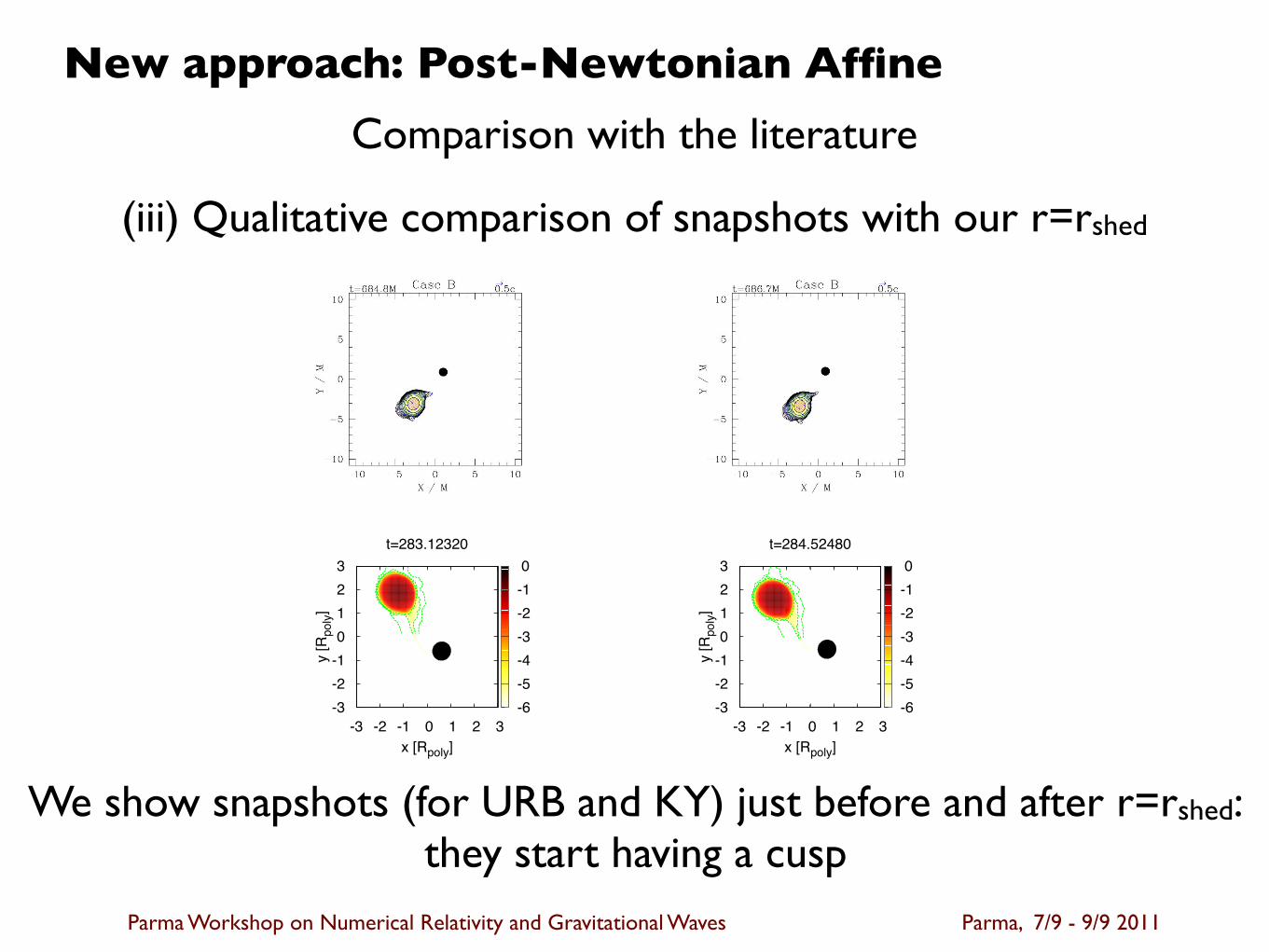
Parma Workshop on Numerical Relativity and Gravitational Waves Parma, 7/9 - 9/9 2011
New approach: Post-Newtonian Affine
Comparison with the literature
(iii) Qualitative comparison of snapshots with our r=rshed
14
t=283.12320
-3 -2 -1 0 1 2 3x [Rpoly]
-3-2-1 0 1 2 3
y [R
poly
]
-6-5-4-3-2-1 0
t=284.52480
-3 -2 -1 0 1 2 3x [Rpoly]
-3-2-1 0 1 2 3
y [R
poly
]-6-5-4-3-2-1 0
t=234.06720
-3 -2 -1 0 1 2 3x [Rpoly]
-3-2-1 0 1 2 3
y [R
poly
]
-6-5-4-3-2-1 0
t=235.46880
-3 -2 -1 0 1 2 3x [Rpoly]
-3-2-1 0 1 2 3
y [R
poly
]
-6-5-4-3-2-1 0
FIG. 3. (Color online) Snapshots of the URB (upper pan-els) and KY (lower panels) simulations, corresponding tot = tshed, evaluated with our approach.
We show snapshots (for URB and KY) just before and after r=rshed:they start having a cusp
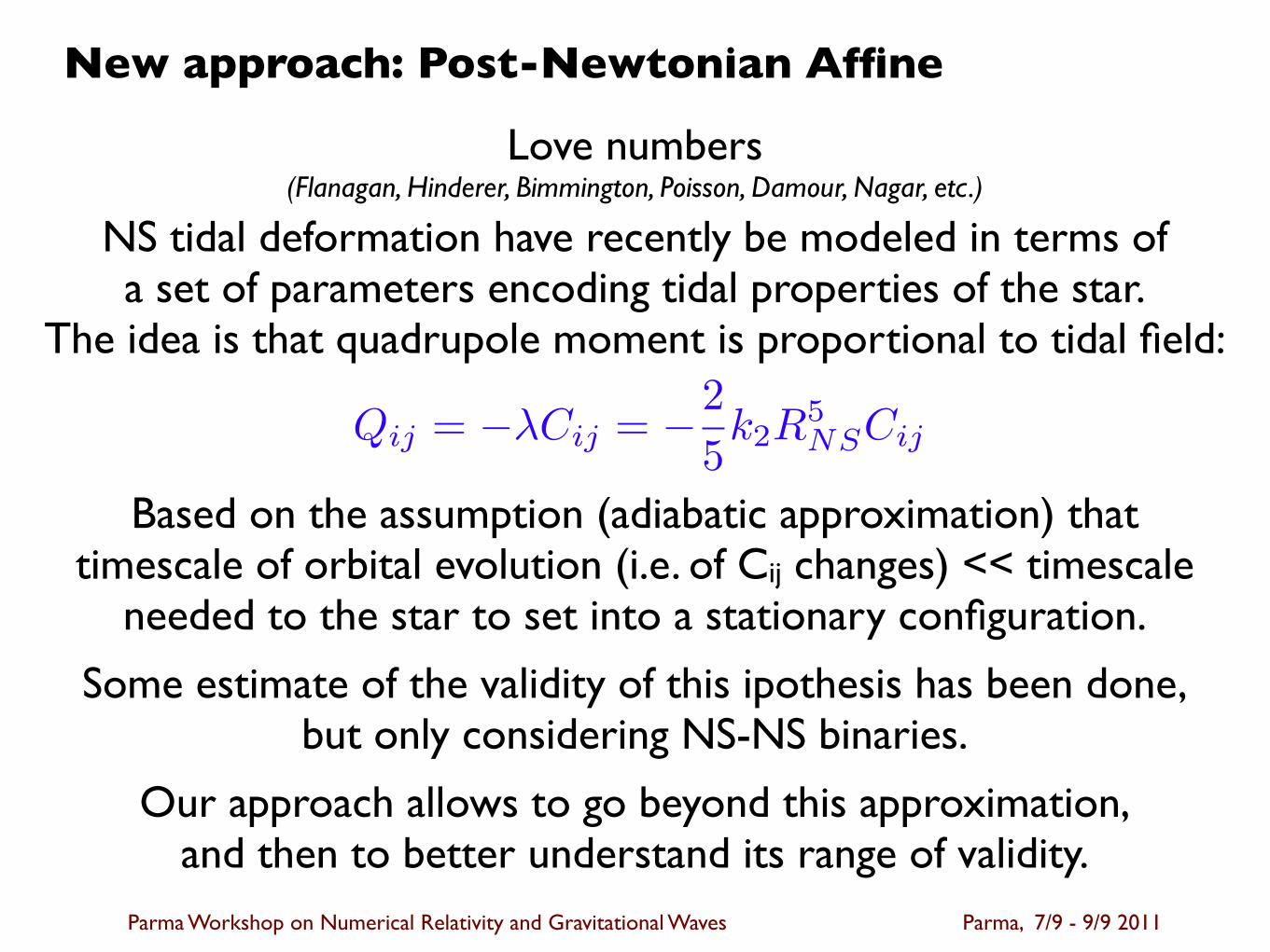
Parma Workshop on Numerical Relativity and Gravitational Waves Parma, 7/9 - 9/9 2011
New approach: Post-Newtonian Affine
Love numbers (Flanagan, Hinderer, Bimmington, Poisson, Damour, Nagar, etc.)
NS tidal deformation have recently be modeled in terms of a set of parameters encoding tidal properties of the star.
The idea is that quadrupole moment is proportional to tidal field:
Qij = −λCij = −2
5k2R
5NSCij
Based on the assumption (adiabatic approximation) that timescale of orbital evolution (i.e. of Cij changes) << timescale
needed to the star to set into a stationary configuration.
Some estimate of the validity of this ipothesis has been done,but only considering NS-NS binaries.
Our approach allows to go beyond this approximation,and then to better understand its range of validity.

Parma Workshop on Numerical Relativity and Gravitational Waves Parma, 7/9 - 9/9 2011
New approach: Post-Newtonian Affine
Love numbers
0.095
0.1
0.105
0.11
0.115
0.12
0.125
40 60 80 100 120 140
k 2
r
q = 2, aBH/MBH = 0, C = 0.15
Love number
C=0.145 q=2
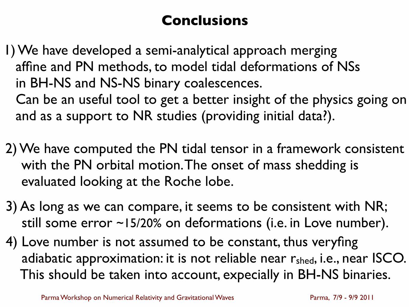
Parma Workshop on Numerical Relativity and Gravitational Waves Parma, 7/9 - 9/9 2011
Conclusions
1) We have developed a semi-analytical approach merging affine and PN methods, to model tidal deformations of NSs in BH-NS and NS-NS binary coalescences. Can be an useful tool to get a better insight of the physics going on and as a support to NR studies (providing initial data?).
2) We have computed the PN tidal tensor in a framework consistent with the PN orbital motion. The onset of mass shedding is evaluated looking at the Roche lobe.
3) As long as we can compare, it seems to be consistent with NR; still some error ~15/20% on deformations (i.e. in Love number).4) Love number is not assumed to be constant, thus veryfing adiabatic approximation: it is not reliable near rshed, i.e., near ISCO. This should be taken into account, expecially in BH-NS binaries.