MasaomiTanaka(NAOJ)

Time-DomainSciencewithSubaru/HSC

• TransientsurveywithSubaru/HSC

• MulC-messengerastronomy

• Future

Time-DomainSciencewithSubaru/HSC

h"p://hsc.mtk.nao.ac.jp/ssp/science/weak-lensing-cosmology/

Masahiro’stalk

SSPTransientsurvey(2016Nov-,COSMOS)HSCtransientworkinggroup:NaokiYasuda,NozomuTominaga,TomokiMorokuma,NaoSuzuki, IchiroTakahashi,TakashiMoriya,KeiichiMaeda,MasakiYamaguchi,etal.

Thedeepest/widesttransientsurveyaseverToday

14.2 Type Ia Supernovae

Figure 14.11.: Expected confidence regions at 68.3%, 95.4%, and 99.7% of the (ΩM , w) plane assuming the flatuniverse. Dotted lines are for SCP Union2 confidence regions and solid lines are for SCP Union2 plus simulated HSCSNe Ia sample. Only statistical errors are included.

Panagia et al. 2006, Ruiz-Lapuente 2004, Di Stefano 2010, Saio & Nomoto 1985, Pakmor et al.2007).

One indirect way to constaint SN Ia progenitor is the Delay Time Distribution (DTD) - thedistribution of the time elapsed from the formation of the binary to the explosion. In SD channel,the delay time is essentially determined by the main-sequence lifetime of the secondary star, hencesome characteristic secondary mass preferred for succsessful SN Ia events lead to a preferred delaytime (Yungelson & Livio 2000, Belczynski et al. 2005). In the other hand, the delay time of DDchannel is mainly determinded by the time scales of gravitational wave radiation. If we assumepower-law distribution of the binary separation, then the form of the DTD become also power-law(see Totani et al. 2008). Then the observed DTD help us to put constraints on SN Ia progenitormodels comparing with theoretical population synthesis studies (e.g., Bogomazov & Tutukov 2009;Ruiter, Belczynski & Fryer 2009; Meng & Yang 2010; Mennekens et al. 2010; Ruiter et al. 2011,for recent studies).

There are many ways to derive DTD from the observation. Since SN Ia rate can be expressed inthe following form, the DTD can be derived when we couple SN Ia rate and star-formation History(SFH) information.

RIa =

! t

0ψ(t − τ)DTD(τ)dτ

Here, RIa(t) is a present SN Ia occurrence rate at some galaxy with age t (or cosmic time when weare concerning about cosmic SN Ia rate), and ψ(τ) is the SFH of the host galaxy (or cosmic SFH).Totani et al.(2008) used SN Ia sample which occured in passive galaxy from Subaru/XMM-NewtonDeep Survey (SXDS) observation, and by combining with nearby SN Ia rate at eliptical galaxy,showed that DTD is well described in featureless power-law as DTD(t) ∝ t−1 in the delay timerange of 0.1-10Gyr. The DTD is derived in various methods: comparing SN Ia rate to cosmic

413

TypeIaSNcosmology High-z“superluminous”SNe

14.5 Type IIn Supernovae

-23-22.5

-22-21.5

-21-20.5

-20-19.5

-19 0 2000 4000 6000 8000 10000

AB m

agni

tude

Rest wavelength (angstrom)

Day 0Day 20Day 40Day 60

Figure 14.20.: SEDs used in the mock simulations. Days are from the maximum luminosity in rest frame. They arebased on the blackbody fit of the SEDs of SN 2008es (SLSN-II, Miller et al. 2009; Gezari et al. 2009).

z = 2.357 is the current record holder of the most distant SN reported (Cooke et al. 2009). Themajor progenitors of SNe IIn are suggested to be luminous blue variables (LBVs) which are in anevolutionary path of very massive stars and undergo extensive mass loss (e.g. Smith et al. 2011;Kiewe et al. 2012). The progenitor of SN IIn SN 2005gl is actually confirmed to be an LBV in thearchval images of HST(Gal-Yam & Leonard 2009; Gal-Yam et al. 2007).

0

20

40

60

80

100

0 1 2 3 4 5 6

N

Redshift

30 deg2

0

5

10

15

20

25

30

0 1 2 3 4 5 6

N

Redshift

3.5 deg2 x 2

Figure 14.21.: Number of the discoveries of SLSN-II estimated by the mock simulations. The left panel is theresult for the 3 month observations with 30 deg2 (deep survey) and the right panel is the result for the 3 monthobservations with two 3.5 deg2 ultra-deep survey areas. Note that the number is expected to be increased more thanroughly 2 times because typical SLSN-II have durations of more than 2 times longer than that of SN 2008es.

14.5.3. SNe IIn Survey with HSC

A main target of HSC SN IIn survey is to determine the rate and the luminosity function of SNe IIn.Although the progenitors of SNe IIn are estimated as stars with the zero-age main-sequence massabove 50 M⊙ (Gal-Yam et al. 2007; Cooke 2008), we still do not have clear ideas of what kindof progenitors explode as SNe IIn. The rate and luminosity function can be a clue to reveal the

427

SCPUnion2+HSC

-TidaldisrupCon=>EvoluConofSMBH-SNrate=>SuccessrateofSN/Progenitorsystem-Newtypesoftransients-…

simulaJonsimulaJon

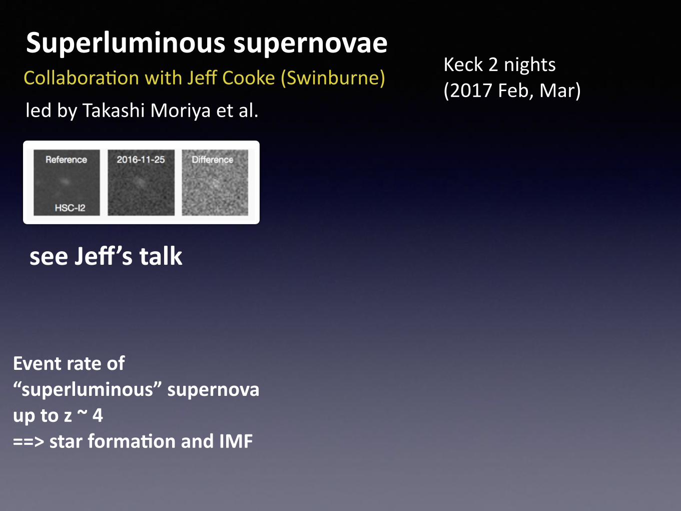
SuperluminoussupernovaeCollaboraJonwithJeffCooke(Swinburne)ledbyTakashiMoriyaetal.

Eventrateof“superluminous”supernovauptoz~4==>starformaConandIMF

Keck2nights(2017Feb,Mar)

seeJeff’stalk

• TransientsurveywithSubaru/HSC

• MulC-messengerastronomy

• Future

Time-DomainSciencewithSubaru/HSC

GravitaConalwaveastronomyAbbo"etal.2016,PRL,061102

=>10-100deg2a]erVirgoandKAGRA

600deg2

900deg2

GW150914=BH-BHmerger

3

16

18

20

22

24

26

28 0 5 10 15 20

-20

-18

-16

-14

-12

-10

Ob

serv

ed

mag

nit

ud

e (

200 M

pc)

Ab

so

lute

mag

nit

ud

e

Days after the merger

g-band

Type Ia SNNS-NSBH-NS

Wind

16

18

20

22

24

26

28 0 5 10 15 20

-20

-18

-16

-14

-12

-10

Ob

serv

ed

mag

nit

ud

e (

200 M

pc)

Ab

so

lute

mag

nit

ud

e

Days after the merger

r-band

Type Ia SNNS-NSBH-NS

Wind

16

18

20

22

24

26

28 0 5 10 15 20

-20

-18

-16

-14

-12

-10

Ob

serv

ed

mag

nit

ud

e (

200 M

pc)

Ab

so

lute

mag

nit

ud

e

Days after the merger

i-band

Type Ia SNNS-NSBH-NS

Wind

16

18

20

22

24

26

28 0 5 10 15 20

-20

-18

-16

-14

-12

-10

Ob

serv

ed

mag

nit

ud

e (

200 M

pc)

Ab

so

lute

mag

nit

ud

e

Days after the merger

z-band

Type Ia SNNS-NSBH-NS

Wind

FIG. 2: Expected observed magnitudes of kilonova models at 200 Mpc distance [70, 71]. The red, blue, and green lines showthe models of NS-NS merger (APR4-1215), BH-NS merger (APR4Q3a75), and a wind model, respectively. The ejecta massis Mej = 0.01M⊙ for these models. For comparison, light curve models of Type Ia SN are shown in gray. The correspondingabsolute magnitudes are indicated in the right axis.

B. NS-NS mergers

When two NSs merge with each other, a small partof the NSs is tidally disrupted and ejected to the inter-stellar medium (e.g., [36, 42]). This ejecta component ismainly distributed in the orbital plane of the NSs. Inaddition to this, the collision drives a strong shock, andshock-heated material is also ejected in a nearly spheri-cal manner (e.g., [48, 84]). As a result, NS-NS mergershave quasi-spherical ejecta. The mass of the ejecta de-pends on the mass ratio and the eccentricity of the orbitof the binary, as well as the radius of the NS or equationof state (EOS, e.g., [48, 84–88]): a more uneven massratio and more eccentric orbit leads to a larger amountof tidally-disrupted ejecta and a smaller NS radius leadsto a larger amount of shock-driven ejecta.

The red line in Figure 1 shows the expected luminosityof a NS-NS merger model (APR4-1215 from Hotokezaka

et al. 2013 [48]). This model adopts a “soft” EOS APR4[89], which gives the radius of 11.1 km for a 1.35M⊙

NS. The gravitational masses of two NSs are 1.2M⊙ +1.5M⊙ and the ejecta mass is 0.01 M⊙. The light curvedoes not have a clear peak since the energy deposited inthe outer layer can escape earlier. Since photons keptin the ejecta by the earlier stage effectively escape fromthe ejecta at the characteristic timescale (Eq. 2), theluminosity exceeds the energy deposition rate at ∼ 5− 8days after the merger.

Figure 2 shows multi-color light curves of the sameNS-NS merger model (red line, see the right axis for theabsolute magnitudes). As a result of the high opacity andthe low temperature [77], the optical emission is greatlysuppressed, resulting in an extremely “red” color of theemission. The red color is more clearly shown in Figure 3,where the spectral evolution of the NS-NS merger modelis compared with the spectra of a Type Ia SN and abroad-line Type Ic SN. In fact, the peak of the spectrum

NS-NS

Diskwind

BH-NS

TypeIaSNi-band,Mej=0.01Msun

1m

4m

8m

MT2016

OpCcalemissionfromGWsources:“kilonova”

DetecConofthecounterpart=>EjecConofr-processelementsSubaru/HSCistheuniqueinstrumentforGWfollow-up

NSNS

r-processnucleosynthesis

(Au,Pt)

ToOtransientsearchforGW151226(BH-BH)Publications of the Astronomical Society of Japan, (2014), Vol. 00, No. 0 3

ing optical-infrared-radio telescopes of Japan.The first direct detection of GW was achieved by aLIGO

on Sep. 14 2015 (Abbott et al. 2016a). aLIGO performedthe first science run (O1) from Sep. 2015 to Jan. 2016. Justbefore the regular operation of O1, aLIGO detected the GWat Sep. 14 2015 09:50:45 UT (Abbott et al. 2016a). TheGW from this event, which was named as GW150914, wasemitted by a 36 M⊙–29 M⊙ binary BH coalescence. Whilemany electromagnetic (EM) follow-up observations were per-formed for GW150914 (Abbott et al. 2016d; Abbott et al.2016e; Ackermann et al. 2016; Evans et al. 2016a; Kasliwal etal. 2016; Lipunov et al. 2016; Morokuma et al. 2016; Serino etal. 2016; Smartt et al. 2016a; Soares-Santos et al. 2016; Troja etal. 2016), no clear EM counterpart was identified with those ob-servations except for a possible detection of γ-ray emission byFermiGammra-ray Burst Monitor (GBM) (Connaughton et al.2016). However, the Fermi GBM detection was not confirmedby INTEGRAL observations (Savchenko et al. 2016).aLIGO detected another GW signal during O1. This event

was detected at 03:38:53 UT on Dec. 26 2015 and was namedas GW151226. The false alarm probability of the event wasestimated as <10−7 (>5σ) and 3.5×10−6 (4.5σ) (Abbott et al.2016c). The GWwas also attributed to a BH–BH binary mergerwhose masses are 14.2+8.3

−3.7 M⊙ and 7.5+2.3−2.3 M⊙. The final BH

mass was 20.8+6.1−1.7 M⊙ and a gravitational energy of ∼1 M⊙

was emitted as GW. The distance to the event was 440+180−190 Mpc

(Abbott et al. 2016c).Here, we report the EM counterpart search for GW151226

performed in the framework of J-GEM. We assume that cosmo-logical parameters h0, Ωm, and Ωλ are 0.705, 0.27, and 0.73,respectively (Komatsu et al. 2011) in this paper. All the photo-metric magnitudes presented in this paper are AB magnitudes.

2 ObservationsWe performed wide-field survey and galaxy targeted follow-up observations in and around the probability skymap ofGW151226. The 90% credible area of the initial skymap cre-ated by BAYESTAR algorithm (Singer et al. 2014) was ∼1400deg2 (LSC and Virgo 2015). The final skymap was refined byLALInference algorithm (Veitch et al. 2015) and the 90% area isfinally 850 deg2 (Abbott et al. 2016c). We also made an integralfield spectroscopy for an optical transient (OT) candidate re-ported by MASTER. The specifications of the instruments andtelescopes we used for the follow-up observations are summa-rized in Morokuma et al. (2016).

2.1 Wide Field Survey

We used three instruments for the wide-field survey; KWFC(Sako et al. 2012) on the 1.05 m Schmidt telescope at Kiso

Fig. 1. The observed area of the wide-field surveys of the J-GEM follow-up observation of GW151226 overlaid on the probability skymap (dark bluescale). Green, red, and yellow colored regions represent the areas observedwith KWFC, HSC, and MOA-cam3, respectively.

Observatory, HSC (Miyazaki et a. 2012) on the 8.2 m SubaruTelescope, and MOA-cam3 (Sako et al. 2008) on the 1.8 mMOA-II telescope at Mt. John Observatory in New Zealand.The KWFC survey observations were done in r-band on

Dec. 28 and 29 and Jan. 1–6 (UT). The total area observedwith KWFCwas 778 deg2 far off the Galactic plane. To performan image subtraction with the archival SDSS (Sloan Digital SkySurvey; Shadab et al. 2015) images, the high probability regionshad to be avoided. Each field was observed typically twice orthree times. The exposure time is 180 sec each and the seeingwas 2.5–3.0 arcsec FWHM.We carried out an imaging follow-up observations with HSC

in the first half nights of Jan. 7, 13, and Feb. 6, 2016 (UT). Weobserved an area of 63.5 deg2 centered at (α, δ) = (03:33:45,+34:57:14) spanning over the highest probability region in theinitial skymap (BAYESTAR) with 50 HSC fiducial pointings.The fiducial pointings were aligned on a Healpix (Gorski, et al.2005) grid with NSIDE=64 (a corresponding grid size is 0.84deg2). To remove artifacts efficiently, we visited each fiducialpointing twice with a 2 arcmin offset. We observed the field ini-band and z-band with an exposure time ranging from 45 secto 60 sec for each pointing. On Feb. 6, first we surveyed all thefields by single exposure, then observed the whole area again.The seeing ranged from 0.5 arcsec to 1.5 arcsec FWHM.We also performed survey observations with MOA-cam3 for

a part of the skymap in the southern hemisphere from UT Mar.8 to 11 2016. The total area covered by the MOA-cam3 ob-servations was 145 deg2. The “MOA-Red” filter (Sako et al.2008), which is a special filter dedicated to micro-lens surveywith a wide range of transmission from 6200A to 8100A wasused. The exposure time per field was 120 sec. The seeing was

64deg2(7%)in0.5night!

HSC:1256candidatesand~60likelyextragalacCctransients=>Needspectroscopyforthesmokinggun

J-GEM(JapanesecollaboraJonforGW-EMfollow-up:Yoshidaetal.)

Yoshida,Utsumi,Tominagaetal.2017,PASJ,69,9

Subaru/HSC

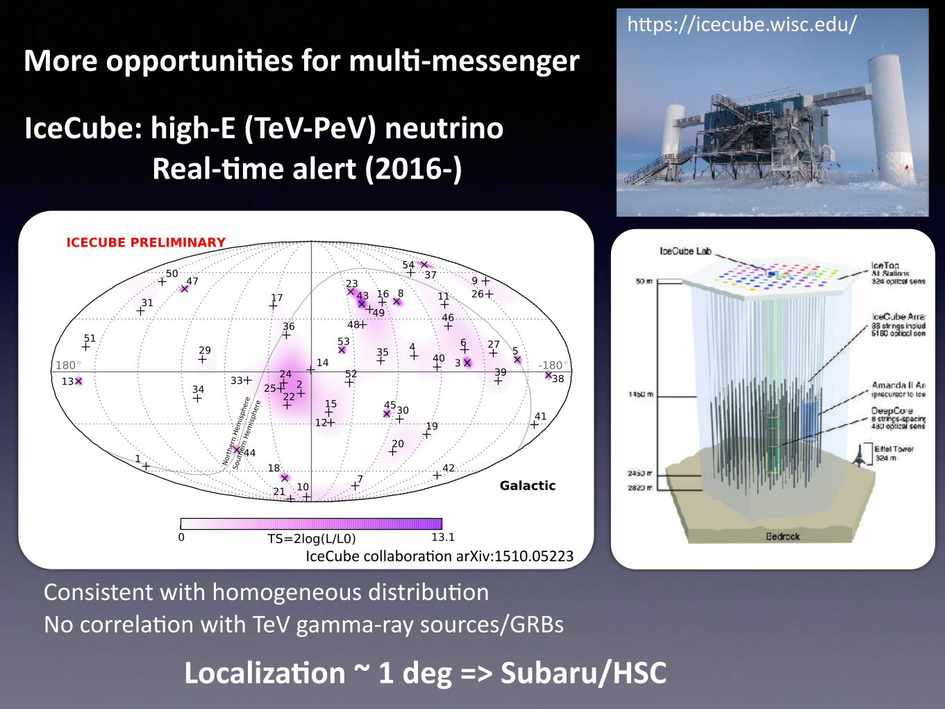
MoreopportuniCesformulC-messenger

LocalizaCon~1deg=>Subaru/HSC

IceCube:high-E(TeV-PeV)neutrinoReal-Cmealert(2016-)

h"ps://icecube.wisc.edu/

Observation of Astrophysical Neutrinos in Four Years of IceCube Data C. Kopper

Figure 7: Arrival directions of the events in galactic coordinates. Shower-like events are marked with +and those containing tracks with . Colors show the test statistics (TS) for the point-source clustering testat each location. No significant clustering was found.

6. Future Plans

Other searches in IceCube have managed to reduce the energy threshold for a selection of start-ing events even further in order to be better able to describe the observed flux and its properties [5],but at this time they have only been applied to the first two years of data used for this study. We willcontinue these lower-threshold searches and will extend them to the full set of data collected byIceCube. Because of its simplicity and its robustness with respect to systematics when comparedto more detailed searches, the search presented here is well suited towards triggering and providinginput for follow-up observations by other experiments. In the future, we thus plan to continue thisanalysis in a more automated manner in order to update the current results with more statistics andto produce alerts as an input for multi-messenger efforts.

References

[1] R. Abbasi et al., Nucl. Instrum. Meth. A601 (2009) 294

[2] M.G. Aartsen et al., Science 342, 1242856 (2013)

[3] R. Abbasi et al., PRL 111 (2013) 021103

[4] M. G. Aartsen et al., PRD89 (2014) 062007

[5] M. G. Aartsen et al., PRD91 (2015) 022001

[6] IceCube Coll., PoS(ICRC2015)1086, these proceedings

[7] IceCube Coll., PoS(ICRC2015)1066, these proceedings

52

ConsistentwithhomogeneousdistribuJonNocorrelaJonwithTeVgamma-raysources/GRBs

IceCubecollaboraJonarXiv:1510.05223

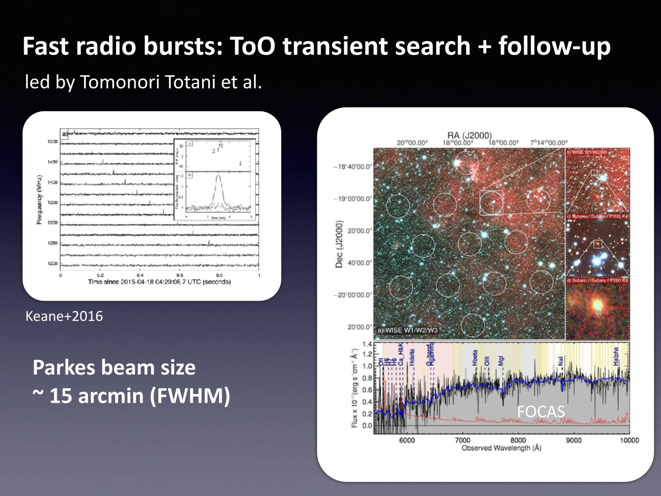
Fastradiobursts:ToOtransientsearch+follow-up

Keane+2016

FOCAS

Parkesbeamsize~15arcmin(FWHM)

ledbyTomonoriTotanietal.

• TransientsurveywithSubaru/HSC

• MulC-messengerastronomy

• Future

Time-DomainSciencewithSubaru/HSC

LSSTScienceBook(aderRau+09,Kasliwal+,Kulkarni+)

4 S. R. KULKARNI CALTECH OPTICAL OBSERVATORIES PASADENA, CALIFORNIA 91125, USA

The sources of interest to these facilities are connected to spectacular explosions. How-ever, the horizon (radius of detectability), either for reasons of optical depth (GZK cuto↵; ! e±) or sensitivity, is limited to the Local Universe (say, distance . 100Mpc). Un-fortunately, these facilities provide relatively poor localization. The study of explosions inthe Local Universe is thus critical for two reasons: (1) sifting through the torrent of falsepositives (because the expected rates of sources of interest is a tiny fraction of the knowntransients) and (2) improving the localization via low energy observations (which usuallymeans optical). In Figure 2 we display the phase space informed by theoretical considera-tions and speculations. Based on the history of our subject we should not be surprised tofind, say a decade from now, that we were not suciently imaginative.

Figure 2. Theoretical and physically plausible candidates are marked in theexplosive transient phase space. The original figure is from Rau et al. (2009).The updated figure (to show the unexplored sub-day phase space) is from theLSST Science Book (v2.0). Shock breakout is the one assured phenomenon on thesub-day timescales. Exotica include dirty fireballs, newly minted mini-blazars andorphan afterglows. With ZTF we aim to probe the sub-day phase space (see §5).

The clarity a↵orded by our singular focus – namely the exploration of the transientoptical sky – allowed us to optimize PTF for transient studies. Specifically, we undertakethe search for transients in a single band (R-band during most of the month and g bandduring the darkest period). As a result our target throughput is five times more relativeto multi-color surveys (e.g. PS-1, SkyMapper).

Given the ease with which transients (of all sorts) can be detected, in most instances, thetransient without any additional information for classification does not represent a useful,let alone a meaningful, advance. It is useful here to make the clear detection betweendetection7 and discovery.8 Thus the burden for discovery is considerable since for most

7 By which I mean that a transient has been identified with a reliable degree of certainty.8By which I mean that the astronomer has a useful idea of the nature of the transient. At the very

minimum we should know if the source is Galactic or extra-galactic. At the next level, it would be useful

FronCeroftransientsky

Depth(Deeper)

Area(Wider)

Cadence(Faster)

3keyparametersofCme-domainsurvey

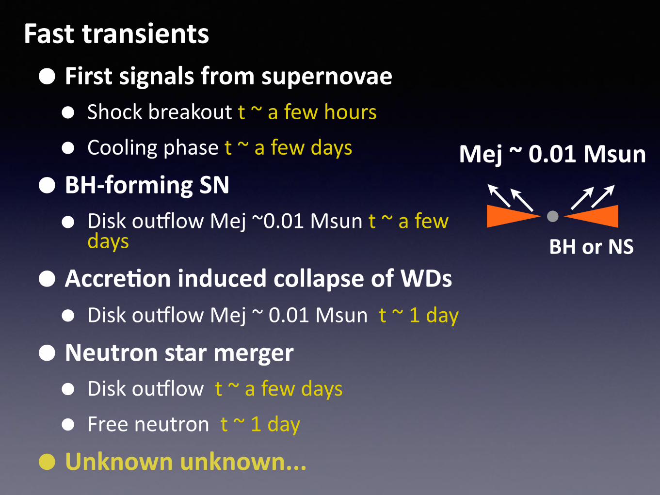
Fasttransients• Firstsignalsfromsupernovae• Shockbreakoutt~afewhours

• Coolingphaset~afewdays

• BH-formingSN• DiskouhlowMej~0.01Msunt~afew

days

• AccreConinducedcollapseofWDs• DiskouhlowMej~0.01Msunt~1day

•Neutronstarmerger• Diskouhlowt~afewdays

• Freeneutront~1day

•Unknownunknown...

BHorNS

Mej~0.01Msun

Pilothigh-cadencesurveywithSubaru/HSC10 Tanaka, M., et al.

-21.0

-20.0

-19.0

-18.0

-17.0

-16.0

-15.0

-14.0

-13.0

-12.0

-11.0 0.1 1 10

0.1 1 10A

bs

olu

te m

ag

nit

ud

e

Rising timescale (day mag-1)

|Δm/Δt| (mag day-1)

14gp (2920A)14or (2620A)14ha (3080A)14jr (3450A)14ef (3060A)

11fe (2600A)

08ax (2600A)

11ht(2590A)

07Y (2590A)

PS1 rapid transients

10aq(2130A)

PS1-13arp(1990A)

06aj t<1d(2520A)

Figure 9. Summary of absolute magnitudes and rising timescale (τrise ≡ 1/ |∆m/∆t|) of transients. Our samples are compared with thefollowing objects: SN 2010aq and PS1-13arp (Gezari et al. 2010, 2015) with early UV detection with GALEX, the early peak of SN 2006aj(Campana et al. 2006; Šimon et al. 2010, ,Figure 6), Type Ia SN 2011fe (Brown et al. 2012), core-collapse SNe (Type Ib SN 2007Y, Type IIbSN 2008ax, and Type IIn SN 2011ht, Pritchard et al. 2014), and rapid transients from PS1 (Drout et al. 2014). For rapid transients fromPS1, the rising timescale (rising rate) is measured with g-band data. The dashed lines show the absolute magnitude and rising timescaleof PS1-10ah and PS1-10bjp measured with the interpolated g-band light curves.

conservative lower limit for the event rate (see below forpossible impact of this assumption).

Then, the free parameter in this analysis is only τi.For simplicity, we assume this parameter is the same (τ)for all the objects by neglecting different redshifts. Here,τ means the duration for which transients show a rapidrise with sufficient brightness so that they are recognizedas rapidly rising transients in our survey. For the twoobjects detected both on Days 1 and 2 (SHOOT14or and14jr), the duration of the emission is about 1.2 days inthe observed frame (0.67 and 0.86 days in the restframe,respectively), and thus, τ is not much shorter than 1 day.A smaller τ is not excluded for the other three objectsbut they do not show clear intranight variability for 1.6-3.1 hr in the observed frame (1.0-2.0 hr in the restframe).Comparison with previously known transients (Section 3)and also with models (see Section 5.2) suggest that it isunlikely that the rising rate as high as |∆m/∆t| > 1 magday−1 continues for > 2 days in restframe with sufficientbrightness. Thus, we adopt τ = 1 day as a fiducial valuefor all objects.

A typical 3σ limiting magnitude for the images used forcandidate selection is ≃ 26.0 mag. We use this value forthe calculation of the maximum volume Vmax. In fact, forobjects to be recognized as rapidly rising transients, theyshould be sufficiently brighter than the limiting magni-tude on Day 2. Thus, the effective limiting magnitude forthe rapidly rising transients tends to be shallower than26.0 mag. Since analysis with a shallower limiting mag-nitude gives a smaller maximum volume and a higher

event rate, our choice of deep limiting magnitude givesconservative estimates for the event rate. It is notedthat the extinction in the host galaxy is not correctedand the true absolute magnitude of our samples shouldbe brighter. However, if the extinction for the currentsamples represents an average degree of extinction, theestimate of Vmax is not significantly affected (i.e., ourestimate crudely includes the effect of extinction).

We estimate pseudo event rate for each object (Ri).For example, the maximum redshift, in which our sur-vey would have detected SHOOT14gp, is zmax = 1.87with the limiting magnitude of 26.0 mag using absolutemagnitude of M = −18.67 mag and crude K-correction(the term of 2.5 log(1 + z)) as in Section 3. The co-moving volume within this redshift in 12 deg2 surveyarea is Vmax,i = 0.16 Gpc3. For this object to be de-tected with our survey, the required event rate should beRi ≃ 1/τiVmax,i ≃ 0.23 × 10−5(τ/1day)−1 yr−1 Mpc−3.Similar analysis for SHOOT14or, 14ha, 14jr and 14ef givezmax = 1.28, 0.70, 0.82, and 0.62, and the event rates areRi ≃ 0.47, 1.9, 1.3, 2.5 ×10−5(τ/1day)−1 yr−1 Mpc−3,respectively.

By summing up the pseudo rates, the lower limit ofthe total event rate is R ≃ 6.4 × 10−5 (τ/1day)−1 yr−1

Mpc−3. It corresponds to about 9 % of core-collapse SNrate at z ∼ 1 (the core-collapse SN rate is (3− 7)× 10−4

yr−1 Mpc−3 at z = 0 − 1, Dahlen et al. 2004; Botticellaet al. 2008; Li et al. 2011; Dahlen et al. 2012). Notethat the event rate is dominated by the less luminousobject with smaller maximum volumes. The event rate

seealsoOfeketal.;Gezarietal.

ThefirstdayofSN

??SNwith

largemassloss??

MT,Tominaga,Morokuma,Yasuda+2016

=>Coordinatedsurvey&rapidfollow-uparecriCcal

High-cadencetransientsurveywithSubaru/HSC

•Depth:25mag(1minexposure)

•Cadence:1hr+1day

• 10consecuCve0.5nights(open-use)

Day1 2

mag

3

|||| |||| ||||

...10

||||

+Follow-upspectroscopy+Coordinatedsurvey(mulC-wavelength)

Day1 2

mag

...103

|||| |||| |||| ||||

Day1 2

mag

...103

|||| |||| |||| ||||

High-cadencetransientsurveywithSubaru/HSC

•Depth:25mag(1minexposure)

•Cadence:1hr+1day+1month

• 10consecuCve0.5nightsx2(intensive)

+Follow-upspectroscopy+Coordinatedsurvey(mulC-wavelength)

• (1.Myself)Time-domain,transient,andmulJ-messenger(GW,ν)

• (2.On-goingcollaboraCon)SSPtransientsurvey+Keckfollow-up(J.Cooke)

• (3.Short/LongtermcollaboraCon)Short:SSP+follow-up(currentscheme)Long:Dedicatedhigh-cadencetransientsurvey

• (4.Size)~5HSCnights(normal)to~10-20HSCnights(intensive) +spectroscopicfollow-up+mulJ-λcoordinaJon

• (5.Instrument)HSC,nobigdemandfornewinstruments

• (6.OperaCon)Flexiblescheduling=cadenceobservaJonsinqueuemodeInter-partnerToO