Time scales and FSI in unsteady liquid-filled pipe flow Arris S Tijsseling Alan E Vardy Department of Mathematics and Computer Science Civil Engineering Division Eindhoven University of Technology University of Dundee P.O. Box 513, 5600 MB Eindhoven Dundee DD1 4HN The Netherlands United Kingdom ABSTRACT Time scales are used to classify unsteady flow in liquid-filled pipes. Seven types of pipe flow are distinguished, with time scales ranging from infinity to zero. Nothing happens when the time scale tends to infinity: the flow is steady. Everything seems to happen when the time scale tends to zero: all (coupled) modes of vibration of liquid and pipe are excited. The complexity of mathematical models describing the phenomena increases as time scales become smaller. An attempt is made to provide and rationalise characteristic time scales, length scales and natural frequencies. Governing equations for the fluid and structure are given in dimensional form (but eventually should be scaled to find characteristic non-dimensional groups). Illustrating examples are given for accelerating flow, water hammer and FSI in a single pipe. One aim of the present investigation is to find the time scale for which 1D-FSI is of importance. Keywords: rigid column, water hammer, fluid-structure interaction (FSI), pipe stress NOMENCLATURE

P fluid pressure, Pa Scalars PDE partial differential equation

r radial coordinate, m c fluid wave speed, m/s t time, s sc solid wave speed, m/s

zu& axial pipe velocity, m/s D inner diameter of pipe, m E Young modulus of pipe wall material, Pa V cross-sectional average of axial fluid e pipe wall thickness, m velocity, m/s f Fanning or skin friction coefficient; v axial fluid velocity, m/s

w radial fluid velocity, m/s frequency, Hz z axial coordinate, m FSI fluid-structure interaction γ angle between pipe and horizontal, rad Im modified Bessel function of the first kind of

order m ∆P (linear) pressure rise within time ∆t, Pa J0 Bessel function of the first kind of order 0 ∆t duration of excitation, s J1 Bessel function of the first kind of order 1 ∆V (linear) velocity rise within time ∆t, m/s K fluid bulk modulus, Pa λ Darcy-Weisbach friction coefficient: L pipe length, m 4 fλ =

1

λn nth zero of J0 µ Poisson ratio ν kinematic viscosity, m2/s ρ fluid mass density, kg/m3 ρs solid mass density, kg/m3

σhoop hoop stress in pipe wall, Pa σz axial stress in pipe wall, Pa φ circumferential coordinate Subscripts ext_bdys external boundaries

int_bdys internal boundaries r reversal rc rigid column s structure, solid, pipe sh “steel hammer” su start up wh water hammer z axial direction 0 initial steady state ∞ final steady state

1 INTRODUCTION Background The authors have recently participated in a project aimed at the definition of practical guidelines for dealing with fluid-structure interaction in industrial pipe systems. See www.win.tue.nl/fsi. In such a project, it is wise to fall back on basic fluid principles (1). One of these principles is to consider the time scale of the problem at hand. For unsteady flow in pipes, this leads to a natural set of regimes. One of these regimes is water hammer with FSI; this is the regime where pipe motion starts to influence the unsteady flow. The main objective of this paper is to identify this particular time scale within a ranking of time scales associated with flows in pipes that are not fully restrained (i.e. are able to move in response to internal fluid forces). Previous efforts in this direction are described by Lavooij & Tijsseling (2), Uffer (3) and Hamilton & Taylor (4). Scope We consider cylindrical pipes of circular cross-section with thin linearly-elastic walls and filled with weakly-compressible (elastic) liquid. The flow velocities are small (e.g. less than 10 m/s for water in a pipeline), the absolute pressures are above vapour pressure, and pressure variations caused by turbulence and vortex shedding are disregarded, as are surface and electro-magnetic effects. Both one-way (liquid → pipe) and two-way (liquid ↔ pipe) FSI are considered. Outline Section 2 classifies unsteady flows according to time scales (defined in Section 3) and gives relevant governing equations. The FSI mechanisms in each type of flow are explained and the equations needed in a pipe stress analysis are given. Section 3 lists and discusses the characteristic time scales and frequencies. Section 4 illustrates and Section 5 concludes. Appendix A gives a summary of closed-form solutions in rigid-column theory. The Nomenclature defines the symbols; these are not declared in the text. 2 CLASSIFICATION OF FLOW The purpose of this section is to categorise the types of flow that might be encountered in industrial systems and to demonstrate a natural progression from each type to the next. The corresponding flow-induced stresses and FSI mechanisms are described. 2.1 No-flow

2

Fluid The no-flow situation gives the hydrostatic pressure in the pipe system. For a single pipe, gravity defines the pressure according to

sinP gz

ρ∂ =∂

γ (1)

Pipes A similar relation holds for the axial tensile stress in an empty pipe:

s sinz gzσ ρ∂− =∂

γ (2)

However, a static stress analysis is more complicated than a hydrostatic pressure analysis; non-vertical pipes sag under their own weight, causing bending moments and shear forces. The support conditions and the flexibility of bends are crucial in a static stress analysis and the largest load is usually due to thermal expansion. The static analysis of the coupled compression, shear, bending and torsion of pipes and resulting anchor forces can be important, but are not considered herein. Account is taken, however, of hydrostatic pressure loads. FSI In liquid-filled pipes, the hydrostatic pressure at any axial location is counterbalanced by a hoop stress in the pipe wall satisfying the equilibrium condition:

hoop12

D Pe

σ = (3)

which is probably the oldest FSI formula. This hoop stress induces hoop strain and it also induces axial stress and/or strain as a consequence of Poisson contraction. Thus, there is a link between the fluid pressure and the axial stress/strain in the pipe wall. This is a simple form of so-called Poisson coupling (so named because the amplitude of the interaction is proportional to the Poisson contraction ratio µ). A simple form of junction coupling can also exist, namely at an unrestrained closed end where the pressure causes an axial stress in the pipe wall satisfying the equilibrium condition:

14z

D Pe

σ = (4)

The description of these examples of Poisson coupling and junction coupling as "simple" does not imply any difference in principle from "non-simple" cases. It is merely a convenient way of distinguishing them from cases where the coupling causes pipe movements. 2.2 Steady flow Fluid In steady flows, shear forces exist between the fluid and the pipe in addition to pressure forces. The flow is driven by a piezometric pressure gradient and is resisted by skin friction at the pipe wall. The resulting pressure gradient is in equilibrium with gravitational and friction forces, satisfying

0 0sin2

V VP gz D

ρ γ λ ρ∂ = −∂

(5)

Pipes The pipes experience skin friction according to

3

0 0s sin

8z V V

gz eσ ρ γ λ ρ∂− = +∂

(6)

FSI Skin friction acts on the whole of the interface between the liquid and the solid as a distributed axial force. The effect is known as friction coupling. At pipe junctions such as bends and branches directional changes of momentum and pressure changes due to local losses cause local axial forces in the pipe wall proportional to 0 0V Vρ . These are further examples of junction coupling. In a steady flow, however, they do not cause any movement of the pipe (although they sustain static deflection of the pipe). 2.3 Quasi-steady flow Fluid In quasi-steady flows, conditions vary in time, but do so sufficiently slowly for the equations of flow at any instant to be assumed identical to those in a truly steady flow with the same instantaneous mean velocity. At a typical instant, the assumed equation of flow is

sin2

V VP gz D

ρ γ λ ρ∂ = −∂

(7)

Pipes The corresponding equation for the pipe is

s sin8

z V Vg

z eσ ρ γ λ ρ∂− = +∂

(8)

Equations (7) and (8) differ from equations (5) and (6) only in the replacement of the steady velocity V0 by a time-varying velocity V(t). FSI The pipes experience variations in skin friction, pressure gradient, momentum changes and local losses. These progress through a succession of quasi-steady states. They may cause the pipe to deflect, but the movements are too slow to have a significant influence on the fluid flows. The pressures and wall stresses closely satisfy equilibrium relationships. 2.4 Rigid column Fluid When the fluid accelerates too rapidly for inertial forces to be neglected, the unsteady flow ceases to resemble a succession of quasi-steady states. Nevertheless, if the accelerations are sufficiently smooth, the velocities (and pressure gradients) may closely approximate to quasi-steady behaviour, in the sense that the velocity along any particular pipe may be regarded as uniform. In this condition, known as rigid-column behaviour, the governing equation of flow is:

sin2

V VV P gt z

ρ ρ γ λ ρ∂ ∂+ = −∂ ∂ D

(9A)

Pipes For this case, the axial motion of a single pipe satisfies:

s s( )

sin8z zz z V u V uu g

t z eσρ ρ γ λ ρ

− −∂ ∂− = +∂ ∂

& && (10)

4

In practice, supports will usually prevent rigid-body pipe motion so that zu& ≈ 0. FSI In common with quasi-steady flows, pipe movements are assumed to have negligible influence on the fluid flow. The pressures and wall stresses at any location again closely satisfy equilibrium relationships. The actual values of these parameters vary in time, but the equations relating them are the same as those for a simple steady flow. That is, equilibrium is assumed to prevail locally. Analytical solutions Closed-form solutions of Eq (9A) can be obtained for a small number of special cases. These include rigid columns driven by steps and ramps in pressure or velocity; see Appendix A. The solutions give mathematical insight into the combined effects of friction and inertia. They have been used herein to check numerical results. 2.5 Water hammer and 1D - FSI Fluid When sufficiently rapid accelerations occur, fluid compressibility effects come into play and it ceases to be acceptable to neglect non-uniformities in velocity along any particular pipe. It becomes necessary to take explicit account of pressure waves that propagate at the speed of sound c in the liquid. The velocity V(z,t) becomes dependent on the axial position z, and a continuity equation (11) must be considered in addition to the equation of motion (9). That is:

( )sin

2z zV u V uV P g

t z Dρ ρ γ λ ρ

− −∂ ∂+ = −∂ ∂

& & (9B)

21 2 zV P

z t Ecσt

µρ ∂∂ ∂+ =∂ ∂ ∂

(11)

Classical water hammer theory (5) neglects convective terms, takes u in Eq (9B), 0z =&

0zσ = in Eq (11), and assumes c to depend on the support conditions of the pipes. Pipes Similarly, axial-stress waves will propagate at the speed of sound cs in the pipe wall. A stress versus rate-of-strain relationship (12) must be used in addition to the equation of motion (10):

s s( )

sin8z zz z V u V uu g

t z eσρ ρ γ λ ρ

− −∂ ∂− = +∂ ∂

& && (10)

s 2s

1z zus

R Pz t E ec

σt

µρ ρ∂ ∂ ∂− = −∂ ∂&

∂ (12)

FSI In this flow state (i.e. water hammer in a movable pipe), the motion of the fluid is influenced by pipe movements. This is a fundamental difference from all of the above flow states in which equilibrium was assumed to prevail locally between fluid and solid forces. Consider Poisson coupling, for example. The pipe wall expands radially when the internal pressure increases. This effect, modelled quasi-statically through Eq (3), causes the dynamic coupling terms on the right sides of the Eqs (11) and (12). The last terms in the Eqs (9B) and (10), modelling friction coupling, depend on the relative velocity zV . Junction coupling at dead ends, elbows and branches, etc is often modelled as above, Eq (4), assuming local

u− &

5

equilibrium. More generally, however, account may need to be taken of the inertia of additional masses at these locations. Irrespective of additional inertia terms, additional equations (namely continuity) are needed to allow for changes in pipe length caused by the movement of junctions. To summarise, FSI in water hammer involves two-way coupling. Pipe vibrations affect the fluid motion and vice versa. Moreover, this is a fundamentally interactive process, thus explaining why an uncoupled analysis (where fluid force histories are used as input data in a structural dynamics code for the pipes, without coupling back) may give erroneous results. The FSI four-equation model Eqs (9B)-(12) is valid for the axial vibration of straight pipes (1D systems). For the in-plane vibration of planar pipe systems (2D systems), four first-order PDEs describing in-plane lateral motion need to be added. Eight lateral and two torsional first-order PDEs need to be added for the description of general non-planar pipe configurations (3D systems). These additional equations are presented by Tijsseling (6) and Wiggert &Tijsseling (7). 2.6 2D - FSI Fluid and Pipes In 2D models the fluid-pipe system is assumed axisymmetric. The variables, like v(z,r,t) and w(z,r,t), are functions of the radial distance from the central axis of the pipe. The simplest model couples potential flow equations for the fluid to membrane equations for the pipes. The effects of axisymmetric bending stiffness, shear deformation, and rotatory inertia can usually be neglected, because these can be seen only in the vicinities of very steep wave fronts and of anchors. Skalak (8), Lin & Morgan (9, 10), Thorley (11), Bürmann (12, 13) and De Jong (14, Chapter 2) investigated and developed 2D-FSI models. FSI FSI is modelled through pressure, shear, radial stick and axial no-slip conditions at the fluid-solid interface at r = D/2. Frequency-domain analysis shows that infinitely many coupled radial-axial modes of vibration exist. Only two modes have a finite phase-velocity at low frequencies; these correspond to water hammer and “steel hammer” in the 1D-FSI model. 2D-FSI aims at accurate modelling acoustic phenomena. Frequencies in the audible range lead to applications in noise reduction, and in haemodynamics, where the large flexibility of the vessels, the medical importance of shear stresses and the accurate calculation of flow patterns are essential (15-18). 2.7 3D - FSI 3-D FSI is the most general case. The variables, like v(z,r,φ,t), are functions of all cylindrical coordinates. Circumferential (lobar) modes of pipe vibration are of importance. In principle, 3D Navier-Stokes equations (acoustic, without convective terms) for the fluid and full shell equations for the structure are needed to describe high-frequency behaviour. At high frequencies the dynamic behaviour becomes more localised, remote boundary conditions are less important locally, and reflections can often be ignored. Rayleigh surface waves may appear in the solid. In practice, a statistical approach is commonly the best option (19). 3D-FSI might be of significance for highly accurate modelling of curved pipes and for ultrasonic phenomena (as used in wall-thickness measurement and flaw detection).

6

3 TIME SCALES System response time scales Mathematically, a multi-scale (or dimensional) analysis of the governing equations will reveal the relative importance of individual terms as functions of the chosen time scales. Physically, one speaks of response (relaxation, retardation) times in the transition from one physical state to another, or of eigenperiods when this transfer induces vibration (or when vibration is maintained by a driving force). In reality, in observing phenomena, the sampling rate and duration of the observation is important. For example, if the sampling rate is large enough, transient events will not be recorded. Excitation time scales The time scale of the excitation causing unsteadiness is of the utmost importance. Typical excitation time scales might include, for example, (i) the time period of a repetitive input or (ii) the duration of an impact force. System response versus excitation If the time scale of excitation is (much) larger than the time scales of system response not much will happen; the situation will be quasi-steady. To have significant unsteadiness, the time scale of the excitation must be smaller than the time scales of the system. The latter determine the dynamic response of the system. Amplitudes It is not only the time scale that is important, but also the magnitude of excitation and response. It is up to the analyst, what he/she thinks is significant. It is noted that events at smaller time scales (higher frequencies) typically have smaller amplitudes (this follows from an energy consideration) and more damping. Definition The time scales defined below concern system response times and eigenperiods. These have to be compared with the time scale of the excitation. No-flow In the no-flow case, V ≡ 0 and the representative time scale is t = ∞. This case is an asymptotic extreme of steady flow, valid as V0 → 0. Steady flow In steady flow, V is constant and the representative time scale is again t = ∞ (there are no changes). This case is an asymptotic extreme of quasi-steady flow, valid for t → ∞ and V∞ = V. Quasi-steady flow In quasi-steady flow, V varies slowly and the representative time scale is large, but t < ∞. All changes occur sufficiently slowly for inertia effects to be neglected. This case is an asymptotic extreme of rigid column theory; it is valid for t >> 2D/(λV). Rigid column Rigid column theory is valid for time scales of the order of t = 2D/(λV). Inertia significantly impedes changes in velocity, but the elasticity of the liquid can be ignored. This case is the

7

asymptotic extreme of water hammer; it is valid for ∆t >> 4L/c, where L is a representative pipe length and ∆t is the time scale of the excitation. Water hammer and 1D-FSI Representative time scales for water hammer are of the order of t = Lext_bdys/c, where the length scale Lext_bdys represents the distance between external boundaries. These time scales apply whether or not pipe motions are sufficient to merit the use of FSI analyses. If they are, however, smaller time scales may exist because movements of internal boundaries can lead to significant wave reflections that are absent when the pipe does not move. Such pipe motion may occur when, for example, the pipe system has sufficient flexibility and the wave fronts are sufficiently steep to create large unbalanced pressure forces. This consideration leads to time scales of the order of t = Lint_bdys/c, where the length scale Lint_bdys represents the distance between interaction points (junction coupling), for example movable elbows. Although FSI is due to axial motion, the excited pipe system prefers to vibrate in its natural modes, which have axial, lateral and torsional components. Therefore, it is convenient to characterise wave propagation phenomena in terms of natural frequencies. The fundamental frequencies for water hammer are c/(4L) and c/(2L) for open-closed and open-open (or closed-closed) systems, respectively. The fundamental frequencies for axial-pipe vibration are cs/(4L) and cs/(2L) for fixed-free and fixed-fixed (or free-free) straight pipes, respectively. The natural frequencies of lateral and torsional pipe vibration can be found in textbooks on structural dynamics. The natural frequencies of pipe systems strongly depend on the support conditions. They provide a fingerprint of the system’s dynamic behaviour and they may indicate the importance of FSI (20). The 1-D FSI case may be regarded as an asymptotic extreme of 2D-FSI when radial changes occur sufficiently slowly for cross-sectional values to be used. It uses only the two low-frequency modes of the infinitely many modes existing in 2D-FSI models. 2D-FSI The characteristic time scale t is of the order of D/c. The ring frequency

sring

cfDπ

= (13)

is the natural frequency of a radially vibrating hoop (the hoop remains circular at all times). This frequency is high: the ratio hoop/axial, fring/fsh, is about L/D. This is the reason that radial inertia of the pipe wall is neglected in Eq (3) in the 1D-FSI model of Section 2.5 (21, pp. 97-99, pp. 121-135). 3D-FSI The characteristic time scale t is of the order of e/c. The ovalizing frequency is:

oval ring

s

2

5

ef fDDe

ρρ

≈+

(14)

This is the cut-on frequency of the first lobar mode (14, pp. 18-23). This frequency is low with respect to the ring frequency and very low with respect to the defined time scale for 3D-

8

FSI (the interaction between lobar and axial-radial modes becomes significant at high frequencies). Although the influence of lobar modes on axial vibration is small at low frequencies, the phenomenon can sometimes be of importance (22). 4 EXAMPLES To illustrate the relative importance of friction, inertia, elasticity and FSI (Poisson coupling) at different time scales, and to gain insight into the phenomena, calculations have been carried out for accelerating liquid flow in a straight pipe. The dimensional test system is a steel pipe filled with water. Turbulent flow is considered in a 200 m long pipe of 0.8 m inner diameter and 8 mm wall thickness. Laminar flow is considered in a 20 m long tube of 0.8 mm inner diameter. The water has mass density 1000 kg/m3, bulk modulus 2.1 GPa and kinematic viscosity 1 mm2/s. The steel pipe has mass density 7900 kg/m3, modulus of elasticity 210 GPa and Poisson ratio 0.3. The Darcy-Weisbach friction factor in turbulent flow is λ = 0.02. The pressure and stress wave speeds are taken c = 1000 m/s and cs = 5000 m/s. The system is excited by a linearly increasing pressure (or velocity) at one of its ends; the pressure remains zero at the other end. The pressure (or velocity) rise is ∆P (or ∆V) within time ∆t, after which the pressure (or velocity) remains constant; see Figure 1. The time interval ∆t is the important time scale of excitation, which is to be compared with the other time scales listed in the Tables 1 and 2.

Table 1 Representative time scales and frequencies in turbulent flow [Numerical values provided for the particular case of water (V∞=2 m/s, c=1000 m/s) in a

steel pipe (L=200 m, D=0.8 m, cs=5000 m/s)]

Typical time scales Frequencies Eq

start-up suV Lt

Pρ ∞=∆

= 40 s (5, Eq 5-7) (15)

rigid column rc

2 DtVλ ∞

= = 40 s (16A)

water hammer 0.4 s = wh

2 L Ltc c

≤ ≤ 4 = 0.8 s 1.25 Hz = wh4 2c fL L≤ ≤ c = 2.5 Hz (17)

steel hammer

0.08 s = shs s

2 L tc c

≤ ≤ 4 L = 0.16 s 6.25 Hz = ssh4 2

c fL L≤ ≤ sc = 12.5 Hz (18)

ringing sring

cfDπ

= = 2150 Hz (13)

ovalizing oval ring

s

2

5

ef fDDe

ρρ

≈+

= 18 Hz (14)

9

Table 2 Representative time scales in laminar flow [Numerical values provided for the particular case of water (V∞=2 m/s) in a steel pipe

(L=20 m, D=0.0008 m)]

Typical time scales Eq

start-up suV Lt

Pρ ∞=∆

= 0.02 s (5, Eq 5-7) (15)

rigid column 2

rc 32Dtν

= = 0.02 s (16B)

2D 2

2D 4Dtν

= = 0.16 s (19)

Analytical solutions used in the calculations are given in the Appendices A and B. 4.1 Starting turbulent flow Herein, turbulent flow means that skin friction is proportional to the square of the average axial velocity. 2D effects in turbulent flow are not considered. A linear pressure ramp ∆P =

212( / )L D Vλ ∞

(V P ρ∆ = ∆ /

ρ

)c

)

= 0.1 bar is applied to accelerate the liquid column from rest to a final steady-state velocity of V∞ = 2 m/s. Figure 2 shows the velocity history when the time of excitation ∆t = 3600 seconds. The excitation is so slow that after, say, fifteen times trc = 600 seconds the situation is quasi-steady. Because the acceleration starts from zero flow, there is no frictional resistance initially. Figure 3 shows the result for ∆t = 60 seconds, which is of the order of trc = 40 seconds. The quasi-steady solution fails to describe the transition from the initial steady state V0 = 0 m/s to the final steady state V∞ = 2 m/s. Figure 4 shows the result for ∆t = 1 second, which is much smaller than trc = 40 seconds so that the excitation is practically a step load for the rigid column. The water-hammer solution, which is also drawn in the figure, is not distinguishable from the rigid-column solution at this plotting scale. Figure 5 shows results for ∆t = 0.1 seconds, which is of the order of twh = 0.4 seconds. The water-hammer effect is clearly visible at this time scale. The effect is still small because ∆P – equal to the final steady-state friction loss – is small, so that the corresponding velocity jumps

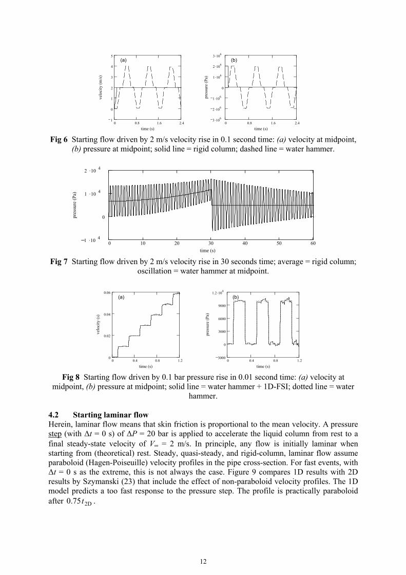
= 0.01 m/s are small too. Water hammer can become spectacular when sudden, large velocity changes exist. In Figure 6, a velocity change ∆V = 2 m/s, again within ∆t = 0.1 seconds, causes a water-hammer pressure = 20 bar. Figure 7 shows the pressure variation caused by the same velocity jump of ∆V = 2 m/s, but now linearly applied over a time period of ∆t = 30 seconds. Rigid column theory gives an initial pressure rise of = 1/15 bar at the pipe midpoint, which also is the initial amplitude of benign water hammer at the midpoint. The figure nicely confirms that rigid column theory gives the time-average of the water-hammer oscillation. Figure 8 shows the equivalent of Figure 5 for ∆t = 0.01 seconds, which is smaller than the time scale for FSI in a single straight pipe: t

P c Vρ∆ = ∆

( ). /(2P V L tρ∆ = ∆ ∆

sh = 0.16 seconds. The pipe is structurally fixed at the excited end and stress-free at the other end. The FSI effect, visible now, is small initially because the interaction consists of Poisson coupling only. In general, junction coupling is a stronger effect.

10

The frequencies in Table 1 confirm that the ring frequency, characterising radial pipe vibration, is much higher than the water-hammer frequency and therefore of negligible importance in 1D-FSI. The frequency of ovalizing vibration has the same order of magnitude as the “steel-hammer” frequency, but there is no significant oval-axial interaction mechanism at these low frequencies.

0 0.5 1 1.5 2 2.5 3 3.5 40

0.5

1

1.5

P t( )∆P

V t( )∆V

t∆t

Fig 1 Pressure (or velocity) ramp excitation at

upstream end of pipe.

0 600 1200 1800 2400 3000 36000

0.5

1

1.5

2

time (s)

velo

city

(m/s

)

Fig 2 Starting flow driven by 0.1 bar pressure

rise in 3600 seconds time; solid line = rigid column; dashed line = quasi steady; dotted line =

frictionless rigid column.

0 20 40 60 80 100 1200

0.5

1

1.5

2

time (s)

velo

city

(m/s

)

Fig 3 Starting flow driven by 0.1 bar pressure

rise in 60 seconds time; solid line = rigid column; dashed line = quasi steady; dotted line =

frictionless rigid column.

0 10 20 30 40 50 60 70 800

0.5

1

1.5

2

time (s)

velo

city

(m/s

)

Fig 4 Starting flow driven by 0.1 bar pressure

rise in 1 second time; solid line = rigid column ≈ dashed line = water hammer; dotted line =

frictionless rigid column.

0 0.4 0.8 1.20

0.02

0.04

0.06

time (s)

velo

city

(m/s

)

0 0.4 0.8 1.23000

0

3000

6000

9000

1.2 .104

time (s)

pres

sure

(Pa)

(a) (b)

Fig 5 Starting flow driven by 0.1 bar pressure rise in 0.1 second time: (a) velocity at

midpoint, (b) pressure at midpoint; solid line = rigid column; dashed line = water hammer.

11

0 0.8 1.6 2.41

0

1

2

3

4

5

time (s)

velo

city

(m/s

)

0 0.8 1.6 2.43 .106

2 .106

1 .106

0

1 .106

2 .106

3 .106

time (s)

pres

sure

(Pa)

(a) (b)

Fig 6 Starting flow driven by 2 m/s velocity rise in 0.1 second time: (a) velocity at midpoint,

(b) pressure at midpoint; solid line = rigid column; dashed line = water hammer.

0 10 20 30 40 50 601 .10 4

0

1 .10 4

2 .10 4

time (s)

pres

sure

(Pa)

Fig 7 Starting flow driven by 2 m/s velocity rise in 30 seconds time; average = rigid column;

oscillation = water hammer at midpoint.

0 0.4 0.8 1.20

0.02

0.04

0.06

time (s)

velo

city

(s)

0 0.4 0.8 1.23000

0

3000

6000

9000

1.2 .104

time (s)

pres

sure

(Pa)

(a) (b)

Fig 8 Starting flow driven by 0.1 bar pressure rise in 0.01 second time: (a) velocity at

midpoint, (b) pressure at midpoint; solid line = water hammer + 1D-FSI; dotted line = water hammer.

4.2 Starting laminar flow Herein, laminar flow means that skin friction is proportional to the mean velocity. A pressure step (with ∆t = 0 s) of ∆P = 20 bar is applied to accelerate the liquid column from rest to a final steady-state velocity of V∞ = 2 m/s. In principle, any flow is initially laminar when starting from (theoretical) rest. Steady, quasi-steady, and rigid-column, laminar flow assume paraboloid (Hagen-Poiseuille) velocity profiles in the pipe cross-section. For fast events, with ∆t = 0 s as the extreme, this is not always the case. Figure 9 compares 1D results with 2D results by Szymanski (23) that include the effect of non-paraboloid velocity profiles. The 1D model predicts a too fast response to the pressure step. The profile is practically paraboloid after . 2D0.75t

12

0 0.02 0.04 0.06 0.08 0.10

0.5

1

1.5

2

time (s)

mea

n ve

loci

ty (m

/s)

Fig 9 Starting laminar flow driven by 20 bar instantaneous pressure rise; solid line = rigid column (1D); dotted line = frictionless rigid column (1D); upper dashed line = 2D-result,

cross-sectional average of velocity; lower dashed line = 2D-result, half the maximum velocity (2D-results by Szymanski (23)).

5 CONCLUSIONS Conditions of no-flow, steady flow, quasi-steady flow, rigid-column flow and water hammer have been described with special reference to (i) coupling between the fluid and the structure and (ii) time scales typifying the key characteristics of the flow. Three types of coupling exist in all types of flow, namely junction coupling, Poisson coupling and friction coupling. The first two of these exist even in no-flow conditions. Notwithstanding the existence of coupling, accurate predictions of pressures and stresses can be obtained from separate (uncoupled) structural and fluid analyses in all types of flow with time scales larger than the water-hammer time scale. The characteristic time scales of no-flow and steady flow are infinite and those for quasi-steady flow are very large. Smaller characteristic time scales apply for rigid column flow, relating primarily to the balance between inertia and frictional resistance. The smallest time scales for 1-D phenomena, namely for water hammer and FSI, are independent of friction (just like no-flow!). They relate to the time taken for waves to travel between adjacent outer boundaries and adjacent inner boundaries respectively. The paper is a first attempt to define time scales for problems possibly involving FSI. The illustrating examples have been kept simple for clarity. Further work should illustrate piping systems with elbows and branches, steady oscillatory flow, resonance behaviour, non-dimensional parameters, 2D-FSI, etc. ACKNOWLEDGEMENT The Surge-Net project (http://www.surge-net.info) is supported by funding under the European Commission’s Fifth Framework ‘Growth’ Programme via Thematic Network “Surge-Net” contract reference: G1RT-CT-2002-05069. The authors of this paper are solely responsible for the content and it does not represent the opinion of the Commission. The Commission is not responsible for any use that might be made of data therein.

13

REFERENCES (1) Vardy AE (1990). Fluid Principles. Maidenhead, UK: McGraw-Hill. (2) Lavooij CSW, Tijsseling AS (1991). Fluid-structure interaction in liquid-filled piping systems. Journal of

Fluids and Structures 5, 573-595. (3) Uffer RA (1993). Water hammer conservatisms. ASME - PVP, Vol. 253, Fluid-structure interaction, transient

thermal-hydraulics, and structural mechanics, 179-184. (4) Hamilton M, Taylor G (1996). Pressure surge – Criteria for acceptability. In Proceedings of the 7th

International Conference on Pressure Surges and Fluid Transients in Pipelines and Open Channels (Editor A Boldy), BHR Group, Harrogate, UK; Bury St Edmunds and London, UK: Mechanical Engineering Publications Limited, 343-362.

(5) Wylie EB, Streeter VL (1993). Fluid Transients in Systems. Englewood Cliffs, USA: Prentice Hall. (6) Tijsseling AS (1996). Fluid-structure interaction in liquid-filled pipe systems: a review. Journal of Fluids

and Structures 10, 109-146. (7) Wiggert DC, Tijsseling AS (2001). Fluid transients and fluid-structure interaction in flexible liquid-filled

piping. ASME Applied Mechanics Reviews 54, 455-481. (8) Skalak R (1956). An extension of the theory of waterhammer. Transactions of the ASME 78, 105-116. (9) Lin TC, Morgan GW (1956a). A study of axisymmetric vibrations of cylindrical shells as affected by rotatory

inertia and transverse shear. ASME Journal of Applied Mechanics 23, 255-261. (10) Lin TC, Morgan GW (1956b). Wave propagation through fluid contained in a cylindrical, elastic shell.

Journal of the Acoustical Society of America 28, 1165-1176. (11) Thorley ARD (1969). Pressure transients in hydraulic pipelines. ASME Journal of Basic Engineering 91,

453-461. (12) Bürmann W (1980). Längsbewegung frei verlegter Rohrleitungen durch Druckstöße. (Longitudinal motion of

pipelines laid in the open due to water hammer.) 3R international 19, 84-91 (in German). (13) Bürmann W (1983). Beanspruchung der Rohrwandung infolge von Druckstößen. (Strain on pipe walls

resulting from water hammer.) 3R international 22, 426-431 (in German). (14) Jong CAF de (1994). Analysis of pulsations and vibrations in fluid-filled pipe systems. PhD Thesis,

Eindhoven University of Technology, Department of Mechanical Engineering, Eindhoven, The Netherlands, ISBN 90-386-0074-7.

(15) Womersley JR (1957). An elastic tube theory of pulse transmission and oscillatory flow in mammalian arteries. WADC Technical Report TR 56-614, Wright Air Development Center, Air Research and Development Command, United States Air Force, Wright-Patterson Air Force Base, Ohio, USA, pp. 1-115 + Appendix.

(16) Cox RH (1969). Comparison of linearized wave propagation models for arterial blood flow analysis. Journal of Biomechanics 2, 251-265.

(17) Stecki JS, Davis DC (1986). Fluid transmission lines - distributed parameter models. Part 1: a review of the state of the art. Part 2: comparison of models. Proceedings of the Institution of Mechanical Engineers, Part A, Power and Process Engineering 200, 215-236.

(18) Rutten MCM (1998). Fluid-solid interaction in large arteries. PhD Thesis, Eindhoven University of Technology, Department of Mechanical Engineering, Eindhoven, The Netherlands, ISBN 90-386-0790-3.

(19) Fahy FJ (1994). Statistical energy analysis: a critical overview. Philosophical Transactions of the Royal Society of London, A 346, 431-447.

(20) Moussou P. Fluid structure interactions in conservative linear systems: a kinematic variational method. Submitted (in 2003) for publication in Journal of Fluids and Structures.

(21) Schwarz W (1978). Druckstoßberechnung unter Berücksichtigung der Radial- und Längsverschiebungen der Rohrwandung. (Waterhammer calculations taking into account the radial and longitudinal displacements of the pipe wall.) PhD Thesis, Universität Stuttgart, Institut für Wasserbau, Mitteilungen, Heft 43, Stuttgart, Germany, ISSN 0343-1150 (in German).

(22) Caillaud S, Lambert C, Devos J-P, Lafon P (2002). Aeroacoustical coupling and its structural effects on a PWR steam line. Part 2. Vibroacoustical analysis of pipe shell deformations. In Proceedings of the 5th International Symposium on Fluid-Structure Interactions, Aeroelasticity, Flow-Induced Vibration and Noise (Editor MP Païdoussis), New Orleans, USA, ASME - AMD, Vol. 253, Paper IMECE2002-33363, pp. 1-8 (CD-ROM, Vol. 3) or ISBN 0-7918-3659-2 (printed book).

(23) Szymanski P (1932). Quelques solutions exactes des équations de l’hydrodynamique du fluide visqueux dans le cas d’un tube cylindrique. (Some exact solutions of the hydrodynamic equations for viscous fluid in the case of a cylindrical tube.) Journal de Mathématiques Pures et Appliquées 11(9), 67-107 (in French).

14

15

16