topology-aware data aggregation for intensive i/o on large...

Context Approach Evaluation Conclusion

Topology-Aware Data Aggregation for Intensive I/O onLarge-Scale Supercomputers

François Tessier∗, Preeti Malakar∗, Venkatram Vishwanath∗,Emmanuel Jeannot†, Florin Isaila‡

∗Argonne National Laboratory, USA†Inria Bordeaux Sud-Ouest, France‡University Carlos III, Spain

January 27, 2017

1 / 23


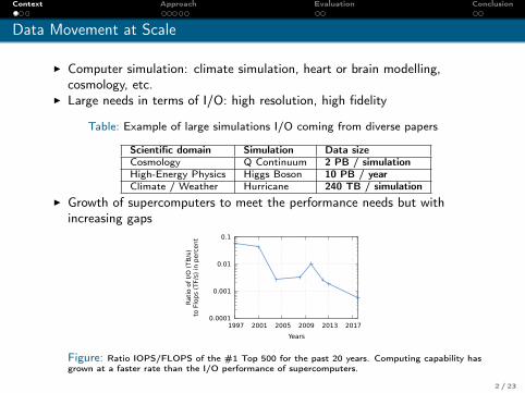
Data Movement at Scale

I Computer simulation: climate simulation, heart or brain modelling,cosmology, etc.

I Large needs in terms of I/O: high resolution, high fidelity

Table: Example of large simulations I/O coming from diverse papers

Scientific domain Simulation Data sizeCosmology Q Continuum 2 PB / simulationHigh-Energy Physics Higgs Boson 10 PB / yearClimate / Weather Hurricane 240 TB / simulation

I Growth of supercomputers to meet the performance needs but withincreasing gaps

0.0001

0.001

0.01

0.1

1997 2001 2005 2009 2013 2017

Rati

o o

f I/O

(TB

/s)

to F

lop

s (T

F/s)

in p

erc

ent

Years

Figure: Ratio IOPS/FLOPS of the #1 Top 500 for the past 20 years. Computing capability hasgrown at a faster rate than the I/O performance of supercomputers.

2 / 23


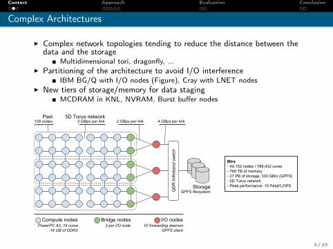
Complex Architectures

I Complex network topologies tending to reduce the distance between thedata and the storage

Multidimensional tori, dragonfly, ...I Partitioning of the architecture to avoid I/O interference

IBM BG/Q with I/O nodes (Figure), Cray with LNET nodesI New tiers of storage/memory for data staging

MCDRAM in KNL, NVRAM, Burst buffer nodes

Compute nodes I/O nodes

Storage

QD

R In

finib

and

switc

h

Bridge nodes

5D Torus network2 GBps per link 2 GBps per link 4 GBps per link

PowerPC A2, 16 cores 16 GB of DDR3

GPFS filesystem

IO forwarding daemon GPFS client

Pset128 nodes

2 per I/O node

Mira- 49,152 nodes / 786,432 cores- 768 TB of memory- 27 PB of storage, 330 GB/s (GPFS)- 5D Torus network- Peak performance: 10 PetaFLOPS

3 / 23


Two-phase I/O

I Present in MPI I/O implementations like ROMIOI Optimize collective I/O performance by reducing network contention and

increasing I/O bandwidthI Chose a subset of processes to aggregate data before writing it to the

storage system

Limitations:I Better for large messages

(from experiments)I No real efficient aggregator

placement policyI Informations about

upcoming data movementcould help

X Y Z X Y Z X Y Z X Y Z

Processes

Data

AggregatorsX X X X Y Y

Y Y Z Z Z Z FileX X X X Y Y

Y Y Z Z Z Z

I/O Phase

Aggr. phase

3210

0 2

Figure: Two-phase I/O mechanism

4 / 23


Outline

1 Context

2 Approach

3 Evaluation

4 Conclusion and Perspectives

5 / 23


Approach

I Relevant aggregator placement while taking into account:The topology of the architectureThe data pattern

I Efficient implementation of the two-phase I/O schemeI/O scheduling with the help of information about the upcomming readingsand writingsPipelining aggergation and I/O phase to optimize data movementsOne-sided communications and non-blocking operations to reducesynchronizations

6 / 23


Aggregator Placement

I Goal: find a compromise betweenaggregation and I/O costs

I Four tested strategiesShortest path: smallest distance to theI/O nodeLongest path: longest distance to theI/O nodeGreedy: lowest rank in partition (can becompared to a MPICH strategy)Topology-aware

How to take the topology into account inaggregators mapping?

Compute node

Bridge node

Storage system

Aggregator

L

S

S

L

Shortest path

Longest path

Greedy

Topology-Aware

Aggregation partition

T

G

G

T

Figure: Data aggregation for I/O:simple partitioning and aggregatorelection on a grid.

7 / 23


Aggregator Placement - Topology-aware strategy

I ω(u, v): Amount of data exchanged betweennodes u and v

I d(u, v): Number of hops from nodes u to v

I l : The interconnect latencyI Bi→j : The bandwidth from node i to node j .

I C1 = max(l × d(i ,A) + ω(i,A)

Bi→A

), i ∈ VC

I C2 = l × d(A, IO) + ω(A,IO)|VC |×BA→IO

Vc : Compute nodesIO : I/O nodeA : Aggregator

C1

C2

Objective function:

TopoAware(A) = min (C1 + C2)

I Computed by each process independently in O(n), n = |VC |8 / 23


Optimized Buffering

I Block of a filesystem: indivisible block of memory on disk requested foreach I/O

I Lock contention avoided in our implementation (in MPI I/O as well)I Simple benchmark with processes writing n × BS (purple) or

n × BS + 1024 (green)

0

5000

10000

15000

20000

1 2 4 8 16 32 64 128

Ave

rage b

andw

idth

(M

Bps)

Data size per rank (in MB)

Impact of the file system block size on I/O2048 Mire-nodes - 1 rank/node - Indep. MPI I/O

Multiple of BSMultiple of BS + 1 KB

I Two pipelined buffers per aggregator (communication overlaped)Aggergation phase: RMA operations (one-sided communications)I/O phase: non-blocking independent write

9 / 23


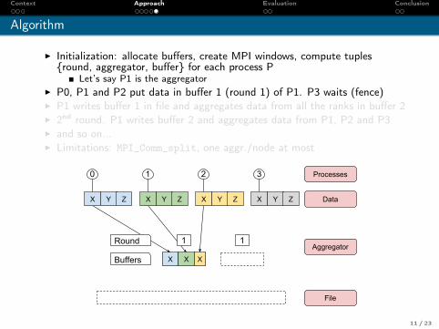
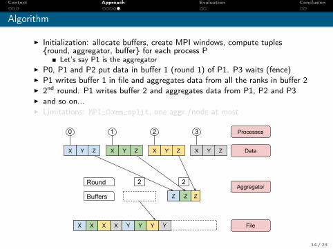
Algorithm

I Initialization: allocate buffers, create MPI windows, compute tuples{round, aggregator, buffer} for each process P

Let’s say P1 is the aggregatorI P0, P1 and P2 put data in buffer 1 (round 1) of P1. P3 waits (fence)I P1 writes buffer 1 in file and aggregates data from all the ranks in buffer 2I 2nd round. P1 writes buffer 2 and aggregates data from P1, P2 and P3I and so on...I Limitations: MPI_Comm_split, one aggr./node at most


Processes

Data

Aggregator

File

3210

Buffers

Round 1 1

10 / 23


Algorithm




Processes

Data

Aggregator

File

3210

Buffers

Round 1 1

X X X

11 / 23


Algorithm




Processes

Data

Aggregator

File

3210

Buffers

Round 1 1

X X X

X Y

12 / 23


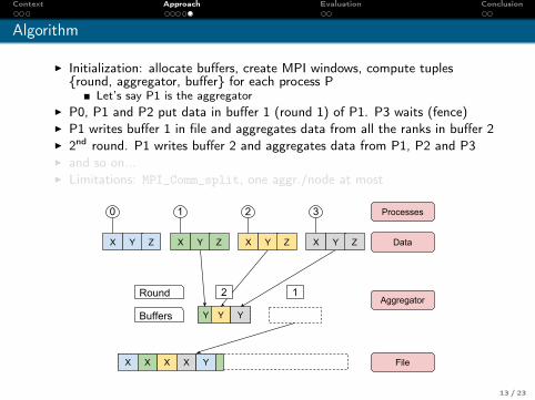
Algorithm




Processes

Data

Aggregator

File

3210

Buffers

Round 1

X X X X Y

Y Y Y

2

13 / 23


Algorithm




Processes

Data

Aggregator

File

3210

Buffers

Round 2

X X X X Y

2

Y Y Y

Z Z Z

14 / 23


Algorithm




Processes

Data

Aggregator

File

3210

Buffers

Round 2

X X X X Y

3

Y Y Y Z Z Z

Z

15 / 23


Algorithm




Processes

Data

Aggregator

File

3210

Buffers

Round 2

X X X X Y

3

Y Y Y Z Z Z Z

16 / 23


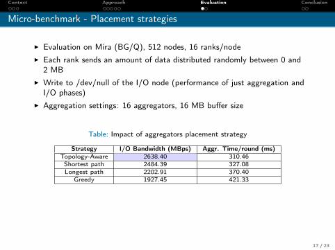
Micro-benchmark - Placement strategies

I Evaluation on Mira (BG/Q), 512 nodes, 16 ranks/nodeI Each rank sends an amount of data distributed randomly between 0 and

2 MBI Write to /dev/null of the I/O node (performance of just aggregation and

I/O phases)I Aggregation settings: 16 aggregators, 16 MB buffer size

Table: Impact of aggregators placement strategy

Strategy I/O Bandwidth (MBps) Aggr. Time/round (ms)Topology-Aware 2638.40 310.46Shortest path 2484.39 327.08Longest path 2202.91 370.40

Greedy 1927.45 421.33

17 / 23


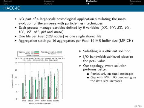
HACC-IO

I I/O part of a large-scale cosmological application simulating the massevolution of the universe with particle-mesh techniques

I Each process manage particles defined by 9 variables (XX , YY , ZZ , VX ,VY , VZ , phi , pid and mask)

I One file per Pset (128 nodes) vs one single shared fileI Aggregation settings: 16 aggregators per Pset, 16 MB buffer size (MPICH)


Processes

Data


Data layoutsin file

X X X X Y Y Y Y Z Z Z Z

Array of structures

Structure of arrays

0 1 2 3

Figure: Data layouts implemented in HACC

18 / 23


HACC-IO




0

1

2

3

4

5

6

5000 15000 25000 35000 50000 100000

Band

wid

th (

GB

ps)

#Particles (38 Bytes/particle)

Write BW comparison according to the strategy and the data size1024 nodes - 16 ranks/node - Single shared file

Topology-aware AoSMPI I/O AoS

POSIX I/O

Topology-aware SoAMPI I/O SoA

I Poor performance in generalI Peak estimated to 22.4 GBps

(theoretical: 28.8 GBps)I Our strategy works better than the

standard ones5K particles and AoS datalayout: 15× faster than MPI I/OVery poor performance fromMPI I/O on AoS

19 / 23


HACC-IO




0

5

10

15

20

25

5000 15000 25000 35000 50000 100000

Band

wid

th (

GB

ps)


Write BW comparison according to the strategy and the data size1024 nodes - 16 ranks/node - One file per pset


POSIX I/O


I Sub-filing is a efficient solutionI I/O bandwidth achieved close to

the peak valueI Our topology-aware solution

performs betterParticularly on small messagesGap with MPI I/O descresing asthe data size increases

20 / 23


HACC-IO




0

10

20

30

40

50

60

70

80

90

5000 10000 15000 25000 35000 50000 100000

Band

wid

th (

GB

ps)


Write BW comparison according to the strategy and the data size4096 nodes - 16 ranks/node - One file per pset


POSIX I/O


I Good scalability on 4K nodesI Similar behavior as on 1024 nodesI I/O bandwidth improved no

matter the data layout andparticularly on messages smallerthan 2 MB

21 / 23


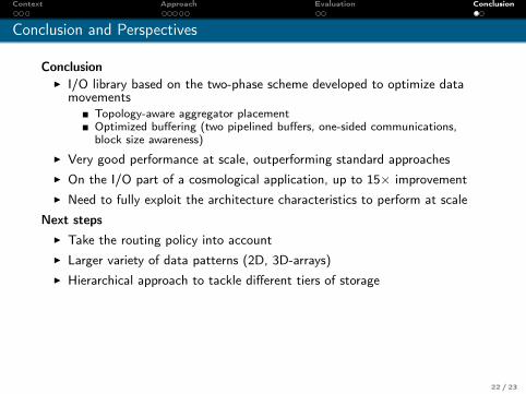
Conclusion and Perspectives

ConclusionI I/O library based on the two-phase scheme developed to optimize data

movementsTopology-aware aggregator placementOptimized buffering (two pipelined buffers, one-sided communications,block size awareness)

I Very good performance at scale, outperforming standard approachesI On the I/O part of a cosmological application, up to 15× improvementI Need to fully exploit the architecture characteristics to perform at scale

Next stepsI Take the routing policy into accountI Larger variety of data patterns (2D, 3D-arrays)I Hierarchical approach to tackle different tiers of storage

22 / 23


Conclusion

Thank you for your attention!

23 / 23

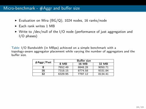
Micro-benchmark - #Aggr and buffer size

I Evaluation on Mira (BG/Q), 1024 nodes, 16 ranks/nodeI Each rank writes 1 MBI Write to /dev/null of the I/O node (performance of just aggregation and

I/O phases)

Table: I/O Bandwidth (in MBps) achieved on a simple benchmark with atopology-aware aggregator placement while varying the number of aggregators and thebuffer size.

#Aggr/Pset Buffer size8 MB 16 MB 32 MB

8 7652.49 8848.28 9050.7116 7318.15 8774.58 9331.8432 6329.95 7797.12 8134.41

24 / 23

topology-aware data aggregation for intensive i/o on large...

Documents