tourism induced contribution to diesel oil and gasoline

[email protected] nº

WP 05/2011

Tourism Induced Contribution to Diesel Oil and Gasoline Consumption

Mohcine Bakhat !Jaume Roselló

2172/8437

Tourism Induced Contribution to Diesel Oil and Gasoline

Consumption

Mohcine Bakhat and Jaume Rosselló1

Mohcine Bakhat is a post-doctoral researcher at Economics for Energy (Spain). Jaume Rosselló-Nadal is an associate researcher of the Economic Research Center and associate professor in the Applied Economics Department of the University of the Balearic Islands (Spain).

1 Acknowledgements: Financial support from the Sixth Framework Program “Climate Change and Impact Research: the

TOURISM INDUCED CONTRIBUTION TO DIESEL OIL AND GASOLINE CONSUMPTION 2

Tourism Induced Contribution to Diesel Oil and Gasoline

Consumption

During the last years, tourism has received increasing attention due to its environmental impacts. Particularly, the

use of fossil energy has been considered as one of its major environmental problems and also one of the factors

directly related to climatic change. Various studies have estimated the contribution of tourism to environmental

damage using a sectorial perspective, evaluating the impact of air transport, the accommodation sector or other

tourism-related economic sector. In this paper, the contribution of tourism to diesel oil and gasoline consumption

is considered from a broader framework, taking advantage of monthly information collected from different

sources. Considering the case study of the Balearic Islands (Spain) and using a conventional econometric model

that includes data for monthly stocks of tourists, the influence of tourism on diesel oil and gasoline demand is

estimated.

Keywords: diesel oil demand, gasoline demand, tourism contribution, environment impacts

Introduction

In the 2007 Davos Declaration, the World Tourism Organization (UNWTO, 2007) acknowledged the two-way relationship between tourism and climate change. Climatic changes will have impacts on a number of tourist destinations and tourist flows. In contrast, tourism is a major contributor to climate change by its use of fossil fuels and emission of greenhouse gases. Thus, mitigate tourism GHG emissions, derived especially from transport and accommodation activities, and apply existing and new technology to improve energy efficiency are therefore important responsibilities for the tourism sector.

Although, awareness about environmental impacts caused by tourism has been increased recently, tourism sector remains a controversial issue in the global sustainable development and climate change. Most environmental concerns in regard to tourism have been connected to the holiday leisure travel sector and few researchers (Becken, 2002b; Høyer & Naess, 2001; Law, 2004) have studied the environmental impacts of tourism. Tourism inevitably contributes to environmental degradation and climate change because large quantities of fossil fuels are required to operate transportation, hotels, and other facilities (Gössling & Svensson, 2006). Lundie, Dwyer and Forsyth (2007) researched an environmental measure of tourism yield by input-output analysis and proved that the major driving factor for energy input is accommodation, causing 16%-29% of the total energy demand. Becken, Simmons and Frampton (2003) also observed key tourism industry subsectors with the highest energy demand, notably transportation, accommodation, and activity in


tourist attractions. Other studies suggested the relevance to research these three subsectors in terms of their onsite impact by energy consumption and transportation (Dubois & Ceron, 2006; Kelly & Williams, 2007).

The biggest drawback to the growth of tourism is its high dependency on transportation. Tourism energy consumption is dominated by transportation (Becken et al., 2003), because “there is no tourism without travel” (Høyer, 2000, p. 147). Air transportation is a primary form of frequent, long-distance travel and is criticized for causing large quantities of greenhouse gas emissions (Becken, 2002a). The Environment Protection Agency (EPA), estimated that for the United States, 76.5% of greenhouse gas emissions of the tourism and recreation sector are caused by transportation (against 15% for lodging, 2.7% for restaurants, 1% for retail, and 4.8% that are activity-specific), and this largely due to the longer air travel distance involved in attending conventions (EPA, 2000).

However, recent studies on social trend showed that tourism is highly influenced by income-driven lifestyles that increase auto-utility and energy use for pleasure and leisure, and thus, people tend to be more concerned with personal convenience than with environmental protection (Ladkin & Weber, 2004; Becken, 2004). On the other hand, with the significant increase of non-package holidays tourist habits worldwide seem to favor a higher number of shorter breaks to short-haul destinations, which in turn leads to increased mobility. And, clearly, the continued growth of low-cost airlines and the increasing use of the Internet will sustain this trend and give more extension to “self-service” tourism (Palmer-Tous, Riera-Font, & Rosselló-Nadal, 2007). Thus, new trends in tourism point towards an increase in tourist mobility in the host country or region, with a subsequent rise in externalities associated with the use of hire cars like atmospheric and noise pollution, congestion and greater numbers of accidents (Banfi, 2000; Nellthorp, Sansom, Bickel, Doll, & Lindberg, 2001; Schreyer, Schneider, Maibach, Rottengatter, Doll, & Schmedding, 2004), and in externalities stemming from the presence of an additional tourist (Palmer & Riera, 2004). Consequently, transportation demand management strategies have become an important issue in regarding sustainable tourism policies in multiple destinations (Carr & Higham, 2001).

Literature Review

The study of automobile fuel consumption is not new. Over the past four decades, many econometric studies have examined the demand for fuel. Whilst the purposes of these studies are diverse, a significant concern has been to analyze the effects on petrol consumption resulting from the threat of fuel energy scarcity (Espey, 1996). More recently, environmental concerns have been cited as a key reason behind the desire to understand and model global fuel demand. It is expected that an increase in price would lead to a decrease in the quantity demanded (a negative price elasticity), and rising income is expected to stimulate petrol usage (a positive income elasticity). Also it can be expected that petrol demand would decline when income decreases, as less transport activities would be required in a less affluent economy. Hence, the assessment of price elasticities and income elasticities has emerged as the centre of many studies to capture the potential effects of price and income changes in fuel demand and car use.

In summary, the most popular approaches and methodologies, such as dynamic reduced form demand models with time series data, have dominated the analysis of price and income elasticities (Prosser, 1985; Sterner, Dahl, & Franzén, 1992, Sterner & Dahl, 1992; Espey, 1998; Goodwin, Dargay, & Hanly, 2004). Other


studies using co-integration techniques have shown that researchers should analyze and take into account the possible non-stationary nature of the time series. Some initial evidence points into the direction that failure to reach stationarity may lead to overestimation of long-run price elasticities (Eltony & Al-Mutairi, 1995; Samimi, 1995; Ramanathan; 1999; Dahl & Kurtubi, 2001). Studies that use disaggregate data have shown that it may be important to provide greater flexibility to the functional forms used for the demand model and, more importantly, that the demographic profiles of households play a major role in automobile fuel consumption (Schmalensee & Stoker, 1999; Yatchew & No, 2001; Kayser, 2000). When demographics are not properly included in the demand model, their effects are partially captured by the income elasticity. The results from disaggregate data seem also better suited to assess the distributional impacts of different policies. Schipper, Figueroa, Espey and Price (1993) showed that there may be strong inaccuracies in the data used in most studies, which may lead to poor estimation of elasticities and erroneous forecasts of future fuel consumption. Finally, structural models of gasoline consumption greatly added to one’s understanding about the exact way in which households and individuals respond to changes in fuel price and income.

Furthermore, the specific nature of the demand functions considered varies depending on a number of factors, but it is generally constrained by the information available or by economic theory. Hence, the endogenous variable (consumption) is frequently considered either in physical units, per capita terms, or taken as energy intensity, defined as the ratio of energy consumption over income. The exogenous variables usually considered are real prices (with or without taxes), real income, structure of production measured either as the index of manufacturing over total output or the ratio of heavy industry over total industry, natural endowment; technology or changes in capital efficiency, climatic differences, etc. (see e.g., Sun, 1998; Liu, 2004; Dees, S., Karadeloglou, Kaufmann, & Sanchez, 2007; Judson, Schmalensee, & Stoker, 1999; Roca & Alcantara, 2002; Zou & Chau, 2006)). Some other studies focus on residential demand, like Leth-Petersen (2002), Kamerschen and Porter (2004), Labandeira, Labeaga and Rodrı’Guez, (2006) and Lenzen (2006). Gasoline demand is also affected by distance driven, the number of vehicles on the road and the fuel efficiency of those vehicles. To take these aspects into account, some authors have directly included in the gasoline demand equation to be estimated, characteristics variables such as vehicle ownership and vehicle fuel efficiency (e.g., Greene, 1982; Baltagi & Griffin, 1983). Some authors have argued that a good way to do this is simply to omit these variables from the model, so that the price elasticity captures the changes in consumption caused by all effects: driving less, changes in vehicle ownership and/or the fuel efficiency of vehicles. A related problem with income elasticity estimates was described by Blum, Foos and Gaudry (1998). They provide some evidence when excluding other exogenous factors affecting travel and ownership, such as weather, availability of infrastructure or public transportation, and economic activities, they can be partially captured in the income elasticity.

Though vehicle characteristics variables are undoubtedly important determinants of gasoline consumption, their inclusion in direct models aimed at analyzing long-run effects appear to be complex. If they are not included in the model, the long-run effects of changes in fuel economy and the stock of cars will be implicitly (although perhaps partially) captured by price and income elasticities.

Although studies on the demand for fuels in industrialized countries is abundant in the economic literature (Schipper, Steiner, Duerr, An, & Strom, 1992; Johansson & Schipper, 1997; Mazzarino, 2000; Kwon, 2005; Polemis, 2006; Tapio, Banister, Luukkanen, Vehmas, & Willamo, 2007; Zervas, 2006; Alvaes & Bueno, 2003;


Samimi, 1995; Ramanathan, 1999; Koshal, Manjulika, Yuko, Sasuke, & Keizo, 2007; Belhaj, 2002) few empirical studies have been done on the Spanish case. Some exceptions are the works of Labeaga and López-Nicolás (1997) and Labandeira and López-Nicolás (2002), which estimate the demand for automotive fuel, though they mainly focus on analyzing the effects of taxes on overall consumption. In another study of Asensio, Matas and Raymond (2002) in which micro data from the Spanish Household Budget Survey was used to estimate the petrol expenditure function for Spain, and the redistributive effects of petrol taxation was evaluated. Pérez-Martínez and Monzón De Cáceres (2006), developed a model for the regions which explains the relationship between greenhouse gas emissions from transportation and the per capita growth in the GDP; Lumbreras, Valdés, Borge and Rodríguez (2008) advanced projections for energy consumption and emissions for the region of Madrid until 2012.

To our knowledge, none of the fuel demand studies or tourism studies so far has used monthly time series data to capture the effect of tourism on fuel demand. The paper is a contribution to the literature to formally test the relationship between tourism and the demand of transportation fuels and particularly diesel oil (type A) and gasoline, taking the case study of Balearics Islands as a geographic isolated territory and highly touristic destination.

The paper is structured as follows. Section 3 considered the model specification and data, including the choice of functional form. Results are then presented in section 4. Conclusions are drawn in the final section.

Demand Model

Data The development of the diesel oil demand model for Balearics islands involves a data constraint and a

prior knowledge from economics. The database gathered covers the monthly demand in thousands of liters for the automobile diesel oil from January 1986 to November 2009 and for gasoline from January 1999 to August 2008. The data is sourced from CHL Company (Compañía Logística de Hidrocarburos) and provided by economic research center of Balearics islands (CRE). Consumer prices after taxes in Euros were available for diesel oil and are taken from official statistics (Mityc, 2010).

The panel (a) in Figure 1 shows the price of diesel and the consumption of diesel in the Balearics islands between 1999 and 2009. During this period diesel consumption in average has increased almost 4 times, and growth was particularly rapid in the period between 1999 and 2006. Between 2006 and 2009, the growth rate slowed down with a less dramatic fashion than in the period before. With respect to Diesel oil price there has been considerable variation between 1999 and 2009, with a minimum value of 0.523€ per liter in February of 1999 and a maximum value of 1.313€ per liter in July 2008. During the period between 1999 and 2004, the diesel oil price was relatively stable, after 2004 the price increased till reaching its maximum in July of 2008, then returned to a relative stability on 2009.

The panel (b) depicts the price and the consumption of gasoline in the Balearics islands between 1999 and 2008. The demand curve follows a negative trend, and during the period of study the gasoline consumption fell some 7% in average. As far as prices are concerned, panel (b) shows as well the fluctuation of gasoline prices between 1999 and 2007 with the minimum value of 0.75€ per liter and the maximum value of 1.16€ per liter that were reported on October 2003 and July 2008 respectively.


Figure 1. (a) Diesel oil price (Euros/liter) and monthly diesel oil consumption (thousands liters) between 1999 and 2009; (b) Gasoline price (Euros/liter) and monthly gasoline consumption (thousands liters) between 1999 and 2007.

Since the aim of this research is to take advantage as much as possible of the information available in a regional scale at a monthly basis. Income, being one of the important exogenous variables, was needed. One of the ideal candidate proxies for income is the real gross domestic product (GDP), which is only available on a quarterly basis, and for this case of study, data were taken from the research centre of Balearics islands (CRE), and they are available online (CRE, 2010). Therefore, some procedure is needed to transform the quarterly measurements into monthly ones. The construction of monthly GDP is carried out by means of cubic spline interpolation method (Weisstein, 2010).

When it comes to tourism, experts faced the problems of measuring the size of this sector and particularly its contribution to the economy. The implementation of the so-called tourism satellite account (TSA) helped to measure the true size of the tourism industry and to show that tourism is a significant part of the overall economy rather than a minor economic player. TSA’s rely on extracting tourism-related economic activity from existing systems of economic accounts, and generally cover only the direct effects of tourism spending in tourism-related industries. Another substantial approach to measure the economic impact of tourism may be labeled “visitor survey method” which relies on more directly estimating tourism volumes and spending via formal visitor surveys. Survey methods often use regional economic tools such as input-output models and multipliers to convert tourist spending to the associated income and jobs and to estimate secondary impacts (multiplier effects). Based on tourism definition, both approaches consider tourism in its disaggregated form and the analysis is usually implemented for tourism related sectors. However, the mixed nature of some sub-sectors of tourism unable many businesses to distinguish sales to locals from sales to tourists. Also, wide variations across seasons and individual businesses, along with non-response problems complicate attempts to estimate tourism industry ratios from industry surveys.

In the aggregated analysis, a researcher may opt for tourist arrivals as a proxy to compute the contribution of tourism on fuel use, nevertheless, this approach with monthly data present two main drawbacks. First, for tourist, the presence of time lag between arrival date and the day when tourist is effectively consuming fuel could result in a bias, and particularly when including tourists arriving at the end of the month. Second, due to


tourism pattern which may change during years, length of stay could be affected and hence its omission in the analysis could largely affect the estimated results.

Hence, the arisen interests to have an accurate measure that can tackle the limitations mentioned previously and respond better to questions set by researchers in the economical analysis, Riera and Mateu (2007) developed a Human Pressure Daily Indicator (HPDI) for the Balearic Islands. This indicator captures the stock of people, at a daily level, on each one of the Balearic Islands, based on resident population data and arrivals and departures from the airports and ports. HPDI takes in consideration the resident population on the first day of each year, and the daily difference between arrivals and departures collected from airport and port statistics, in addition to the natural growth of the population as a consequence of births and deaths.

Given the special purposes of this study, the HPDI is divided into two sub-categories, one for the resident population (HPDI_R) and the second for tourist population (HPDI_T) which facilitate the isolation of the effect of tourism from the residential population (Bakhat, Rosselló, & Sáenz-de-Miera, 2010). This separation is based on Familitur data, the Spanish domestic tourism survey, from which it is possible to estimate how many residents in the Balearics are away on holiday. For the time period of the analysis, the plot for monthly HPDI_R and HPDI_T is shown in Figure 2.

Figure 2. Monthly HPDI for the residents and for the tourists in the Balearics.

One of the most important results that can be derived from this analysis is the fact that tourists account for an average of 25.08% of the total population.

Models Static model: The simplest reduced-form model is static, where fuel demand is specified as a function of

real fuel price and real income. Usually variables are per capita—given the use of the aggregated data—and deflated. Formally, static models are specified as:

Gt = α + β1*Pt + β2*GDPt (1)


Where P and GDP are real price and deflated GDP respectively; and where deflate GDP is used as a proxy to the real income, t is the time of the period under study, and α, β1 and β2 are the parameters to be estimated. Depending on the purpose of the study different log transformation can be done to get the suitable model. In this section, using equation (1), we first present a static model to study the influence of the economic and demographic factors on automobile diesel oil and gasoline consumption separately. The proposed log-linear static model is:

ln(Gt) = α + β1*Pt + β2*GDPt + β3*HPDI_R + β4*HPDI_T + εt (2) where HPDI_R and HPDI_T are variables that represent the pressure of the resident population and tourist population respectively, α, and βi (1≤ i ≤4) are parameters to be determined, and εt is the error term.

Dynamic model: Fuel demand is dynamic by nature and therefore, as studies pointed out by Johansson and Schipper (1997), changes in the explanatory variables do not lead to simultaneous changes in energy usage, which instead lags behind those changes. This may be due, for example, to persistence in fuel usage habits, requiring that a dynamic model should be specified. Some authors use the so-called endogenous lag model, where the endogenous variable is estimated as a function of the lagging endogenous variable. In this paper, following the equation proposed by Koyck (1954), the lagged diesel oil demand variable is included in the demand function to capture possible inertia in the response/adaptation process:

ln(Gt) = α + β1*Pt + β2*GDPt + β3*HPDI_Rt + β4*HPDI_Tt + δ* ln(G(t-12)) (3) In addition, two artificial steps are added to equation (3), in September of 2005 for diesel oil demand and

in March of 2002 for gasoline demand respectively. A possible explanation of the former is that retail gasoline prices reached its historical level in this month and consumers had to switch to the diesel oil product which remained relatively stable during this month.

In cases where the obtainment of the HPDI is not evident, especially in the case of open territories, tourists’ arrival can be used as a proxy variable to estimate the effect of tourism on fuel use. Similarly, equation (2) and equation (3) are used by substituting HPDI for non-residents by tourists’ arrival and then compared to the performance of the resulting models for diesel oil and gasoline respectively.

Results

The results of the models are reported in the Table 1 and Table 2, and for each model the estimates of the parameters associated with the explanatory variables are given. The adjusted R2, Akaike Info Criterion (AIC) and Schwarz Criterion (SC) were also considered for both static and dynamic models. In addition, the F-test was used for the overall significance of the model and a t-test for testing the strength of each of its individual coefficients. The Lagrangian multiplier (LM) test of order 13 has been used to check the presence of correlation between residuals in both static and dynamic models. Furthermore, stability tests were implemented showing no distortion in the parameter estimates. Thus, the results obtained allow concluding that the explanatory variables considered are globally significant in explaining the behavior of the endogenous variable. The adjusted R2 of the estimated models can be qualified as good, being higher than 0.89 for diesel oil and gasoline models. In addition, a subset of variables in the models was tested for statistical significance to examine whether they could be omitted. Each of the insignificant variables was sequentially deleted, using the general-to-specific-model strategy, while significant parameters at 1%, 5% and 10% level were retained.

Diesel Oil Consumption Models


Respectively for models with HPDI variable and tourists’ arrival variable, both real price and GDP are significant with an expected negative sign for the price parameter estimate, and both estimates are consistent with the economic theory. The parameter estimated for endogenous lag variable is positive and significantly different from zero at 1% level of significance. The estimate ranges between 0.19 and 0.21 which is less than 1 confirming in a hand the positive effect of the lag endogenous variable and the evidence of a long run convergence for the diesel oil consumption. The estimate indicates that the rate of convergence is between 19% and 21% which is consistent with the values found in the empirical work of Prosser (1985) for OECD countries, and which explained by the short memory of the consumers.

Table 1 Estimated Models for Diesel Oil Consumption in the Balearics

Hpdi Tourists Static Dynamic Static Dynamic

HPDI_T 2.49E-08*** 1.91E-08*** - - HPDI_R 2.73E-08*** 2.15E-08*** 1.23E-08*** 9.82E-09** Tourists arrivals 3.10E-07*** 2.47E-07*** Constant 9.253*** 7.158*** 10.285*** 8.172*** P -0.748*** -0.869*** -0.965*** -0.942*** GDP 0.009*** 0.010*** 5.07E-03** 0.007*** LOG(Gt-12) 0.213*** 0.194*** Step_2005 0.368*** 0.349202*** 0.358*** Equation statistics Adjusted R2 0.897 0.938 0.926 0.931 Log likelihood 122 146.5 137.396 141.252 Durbin-Watson stat 1.953 1.702 2.034 1.940 AIC -2.572 -3.067 -2.888 -2.951 SC -2.434 -2.874 -2.722 -2.757 F-statistic 197.4 230.5 225.736 203.581 Proba (F-statistic) 0.000 0.000 0.000 0.000 LM(13) 0.690 1.890 4.440 2.720

Notes. *** significant at 1%, ** significant at 5%.

As for population stock variables, both the static and dynamic models show a high significance level for both residents and non-residents. As expected, positive signs are obtained, confirming that an increase in the population (residents or non-residents) will be associated with an increase in diesel oil consumption. The estimates concerning the whole sample period do not differ much between static and dynamic models in the equilibrium. For the dynamic model, in the long run equilibrium, the estimates are 2.42E-08 and 2.73E-08 for non-residents and resident respectively, whereas for static model their correspondents are 2.49E-08 and 2.73E-08. Table 1 reports also the results of static and dynamic models that incorporate tourists’ arrival variable, which shows a high significance jointly with real price, GDP and lag of diesel oil consumption. For the disturbance terms, no presence of serial autocorrelation in the residuals of the dynamic model has been detected. However, by a comparison of the adjusted R squared, Akaike Info Criterion (AIC) and Schwarz Criterion (SC) indicates that the dynamic model incorporating HPDI variable fits well the data and outperforms the model that considers the tourists’ arrival. It is relevant to mention that the estimates of HPDI corresponding to non-residents (Tourists) and tourists’ arrival are


not comparable. In fact, the former estimates the stock of tourists in the islands, in other words, entries minus exits of tourists plus a constant, whereas the tourists’ arrival represents the flow or entries of tourists to the islands.

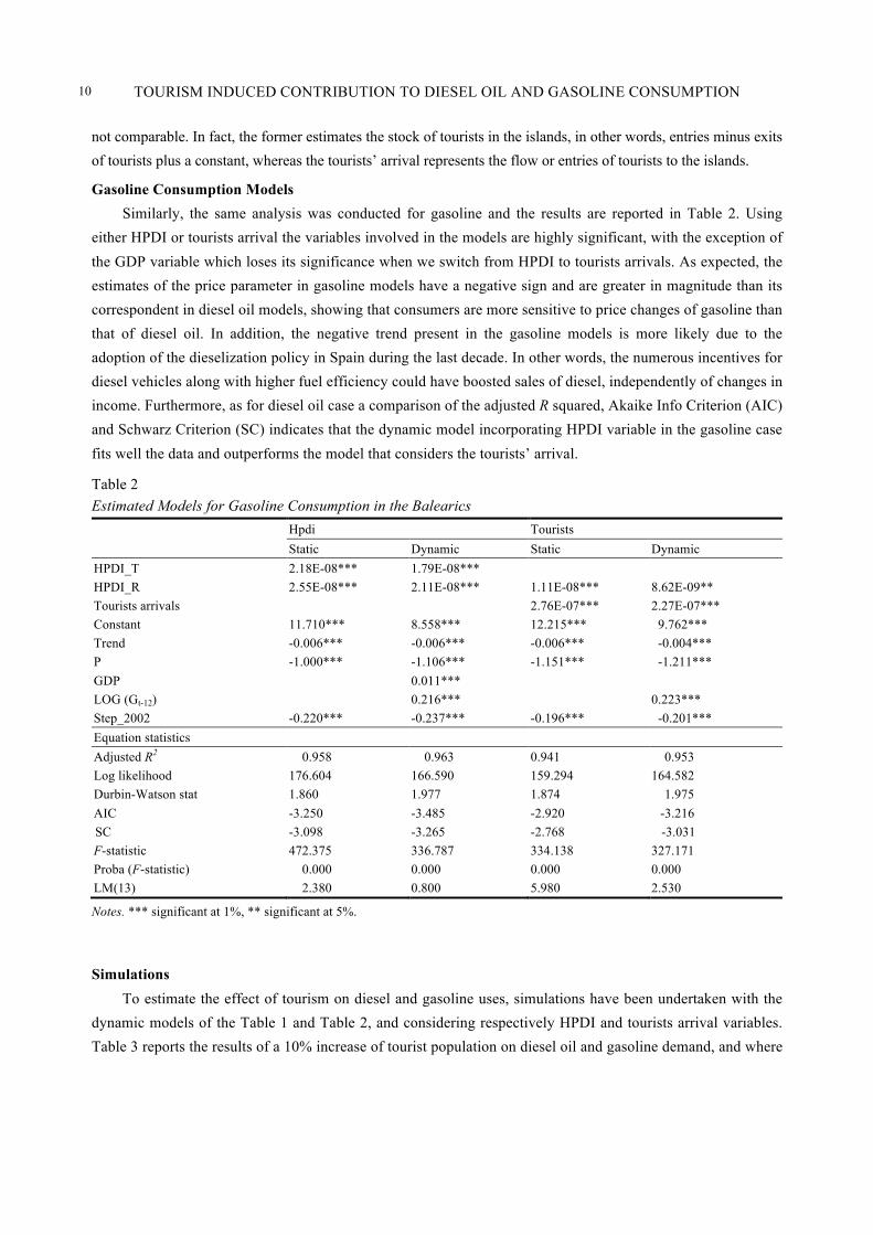
Gasoline Consumption Models Similarly, the same analysis was conducted for gasoline and the results are reported in Table 2. Using

either HPDI or tourists arrival the variables involved in the models are highly significant, with the exception of the GDP variable which loses its significance when we switch from HPDI to tourists arrivals. As expected, the estimates of the price parameter in gasoline models have a negative sign and are greater in magnitude than its correspondent in diesel oil models, showing that consumers are more sensitive to price changes of gasoline than that of diesel oil. In addition, the negative trend present in the gasoline models is more likely due to the adoption of the dieselization policy in Spain during the last decade. In other words, the numerous incentives for diesel vehicles along with higher fuel efficiency could have boosted sales of diesel, independently of changes in income. Furthermore, as for diesel oil case a comparison of the adjusted R squared, Akaike Info Criterion (AIC) and Schwarz Criterion (SC) indicates that the dynamic model incorporating HPDI variable in the gasoline case fits well the data and outperforms the model that considers the tourists’ arrival.

Table 2 Estimated Models for Gasoline Consumption in the Balearics

Hpdi Tourists Static Dynamic Static Dynamic

HPDI_T 2.18E-08*** 1.79E-08*** HPDI_R 2.55E-08*** 2.11E-08*** 1.11E-08*** 8.62E-09** Tourists arrivals 2.76E-07*** 2.27E-07*** Constant 11.710*** 8.558*** 12.215*** 9.762*** Trend -0.006*** -0.006*** -0.006*** -0.004*** P -1.000*** -1.106*** -1.151*** -1.211*** GDP 0.011*** LOG (Gt-12) 0.216*** 0.223*** Step_2002 -0.220*** -0.237*** -0.196*** -0.201*** Equation statistics Adjusted R2 0.958 0.963 0.941 0.953 Log likelihood 176.604 166.590 159.294 164.582 Durbin-Watson stat 1.860 1.977 1.874 1.975 AIC -3.250 -3.485 -2.920 -3.216 SC -3.098 -3.265 -2.768 -3.031 F-statistic 472.375 336.787 334.138 327.171 Proba (F-statistic) 0.000 0.000 0.000 0.000 LM(13) 2.380 0.800 5.980 2.530

Notes. *** significant at 1%, ** significant at 5%.

Simulations To estimate the effect of tourism on diesel and gasoline uses, simulations have been undertaken with the

dynamic models of the Table 1 and Table 2, and considering respectively HPDI and tourists arrival variables. Table 3 reports the results of a 10% increase of tourist population on diesel oil and gasoline demand, and where


the effects are showed by season and for short and long run. For diesel oil consumption, the growth rates corresponding to the different dynamic models (with HPDI or Tourists’ arrival) are quiet similar during the high season (3.4% in the short run for both models and 4.6% and 4.5% in the long run for the two models respectively). However, the differences between the growth rates start to be more noticeable in low and medium seasons with this order of importance. As an example, in the short run, the growth rates in low season are 1.3% and 0.9% respectively, with a difference of 0.4% that tends to increase when we shift to medium season.

Table 3 A Simulation for 10% Increase of Tourists Population and Its Corresponding Effects on Diesel and Gasoline Consumption

Model with tourists arrival Model with HPDI Short-term Long-term Short-term Long-term

Diesel oil High 3.4% 4.5% 3.4% 4.6% Medium 2.4% 3.2% 0.6% 1.0% Low 0.9% 1.7% 1.3% 2.4%

Gasoline High 2.9% 1.9% 3.4% 2.6% Medium 1.1% -0.5% 0.6% -1.0% Low 1.0% -0.1% 1.0% -0.1%

Similarly, gasoline demand shows a small difference of the growth rates between the two models. In high and low seasons 0.5% and 0% are reported respectively, whereas in the medium season this difference tends to increase. Another important result is present in the similarity of the growth rates when we compare diesel oil models to gasoline models in the short-run, and especially for high and low seasons. For instance, in the short-run, the model that incorporates the HPDI variable has the same growth rate in high season (3.4%), whereas in low season 1.3% and 1% are reported for diesel and gasoline respectively. In other words, tourists’ fuel demand is insensitive to current price changes, at least in the short term and with the current simulation.

In order to estimate tourism’s share of total diesel oil and gasoline consumption in the Balearic Islands, a simulation was performed with the absence of the tourist population, considering a time period that ranges from March 2000 to September 2007. The results revealed that a small difference is observed (using either HPDI or tourists’ arrival) between the growth rates associated to diesel oil and gasoline consumption respectively. In the short run, the obtained values range between 22% and 27% for diesel oil consumption, and between 20% and 28% for gasoline consumption. These percentage rates contrast with the proportion of the tourists’ population in Balearics Islands which is estimated at 25% of the total stock.

Conclusions

One of the main drawbacks to the growth of tourism is its high dependency on transportation. Tourism based on air transportation has received the major part in the literature because it is the most environmentally harmful form of tourism with respect to climate change. However, the new trends in tourism which point towards an increase in tourist mobility in the host country or region, aroused interest in researchers to focus their studies on road transportation and its associated externalities. Literature reveals that the costs associated


with tourism have been evaluated from a sectorial perspective, given the non-recognition of the tourist sector in conventional public economic accounting.

The model used in this paper is based on the conventional aggregated models, with the particularity of the inclusion of the population stock variable, whose added endogenous variable is the monthly population stock. Using the case study of the Balearic Islands, which is a highly touristic destination and an isolate territory, a stock of tourist population was developed to be included in the model. In addition, an alternative model was proposed for open territories and where tourists’ arrival was used as a proxy to capture the effect of tourism on fuels use.

Furthermore, either in models which consider HPDI or tourists’ arrival, the results revealed that the explanatory variables and particularly the population stock variables and tourists’ arrival are globally significant in explaining the behavior of the fuels use. Akaike Info Criterion (AIC) and Schwarz Criterion (SC) measures show that for both diesel oil and gasoline the incorporation of HPDI variable instead of tourists’ arrival improves the statistical performance of the models. In addition, simulations have been undertaken considering respectively HPDI and tourists arrival variables, and the effects were showed by seasons and for short and long run. For diesel oil, either in the short or long run the effect of 10% increase of tourists’ population is almost equal during the high season. For instance, during the high season, a 10% increase of tourists’ population corresponds to 3.4% increase of diesel oil consumption in the short run (using either HPDI or tourists arrival), whereas a small difference is observed in the long run (4.6% with models that involve HPDI and 4.5% for its correspondent with tourists arrival variable).

Similarly, results obtained for gasoline demand show a small difference of the growth rates between the two models (using either HPDI or tourists arrival). In addition, and in the short run, growth rates of diesel oil and gasoline are quiet similar and especially for high and low seasons. As an example, in the short-run, diesel and gasoline models that incorporate the HPDI variable have the same growth rate in high season (3.4%), whereas in low season, 1.3% and 1% are reported for diesel and gasoline respectively. In other words, tourists’ fuel demand is insensitive to current price changes, at least in the short term and with the current simulation.

Additionally, it is relevant to mention that the limitation of this study arise in the fact that a complex relationship does exist between tourism; economic growth and diesel oil demand. Changes in GDP could be due to the changes in the tourism activity which is the main economic sector in the Balearics Islands. However, other sectors could also affect GDP independently from tourism. Thus, we assume in this study, that tourism has a direct effect on diesel oil demand, whereas the effect of other sectors is induced by the GDP variable in the specification model.

References Alvaes, D., & Bueno, R. (2003). Short-run, long-run and cross elasticities of gasoline demand in Brazil. Energy Economics, 25,

191-199. Asensio, J., Matas, A., & Raymond, J. L. (2002). Petrol expenditure and redistributive effects of its taxation in Spain.

Transportation Research Part A, 37, 49-69. Bakhat, M., Rosselló, J., & Sáenz-de-Miera, O. (2010). Developing a daily indicator for evaluating the impacts of tourism in

isolated regions. European Journal of Tourism Research, 3(2), 114-118. Baltagi, B. A. G. J. (1983). Gasoline demand in the OECD: An application of pooling and testing procedures. European Economic

Review, 22, 117-137.


Banfi, S. (2000). External costs of transport-accident, environmental and congestion costs in Western Europe. Zurich, INFRAS/IWW.

Becken, S. (2002a). Analyzing international tourists flow to estimate energy use associated with airtravel. Journal of Sustainable Tourism, 10(2), 114-131.

Becken, S. (2002b). The energy costs of the ecotourism summit in Quebec. Journal of Sustainable Tourism, 10(5), 454-456. Becken, S. (2004). How tourists and tourism experts perceive climate change and carbon-offsetting schemes. Journal of

Sustainable Tourism, 12(4), 332-345. Becken, S., Simmons, D. G., & Frampton, C. (2003). Energy use associated with different travel choices. Tourism Management,

24, 267-277. Belhaj, M. (2002). Vehicle and fuel demand in Morocco. Energy Policy, 30, 1163-1171. Blum, U., Foos, G., & Gaudry, M. (1988). Aggregate time series gasoline demand models: Review of the literature and new

evidence for West Germany. Transportation Research A, 22, 75-88. Carr, A., & Higham, J. (2001). Ecotourism: A research bibliography. Department of Tourism, School of Business. Dunedin, New

Zealand, University of Otago. Dahl, C., & Kurtubi. (2001). Estimating oil product demand in Indonesia using a co-integration error correction model. OPEC

review, 25(1), 1-21. Dees, S., Karadeloglou, P., Kaufmann, R. K., & Sanchez, M. (2007). Modelling the world oil market: Assessment of a quarterly

econometric model. Energy Policy, 35(1), 178-191. Dubois, G., & Ceron, J. (2006). Tourism and climate change: Proposals for a research agenda. Journal of Sustainable Tourism,

14(4), 399-415. Eltony, M., & Al-Mutairi, N. (1995). Demand for gasoline in Kuwait: An empirical analysis using cointegration techniques.

Energy Economics, 17, 249-253. Epa. (2000). A method for quatifying environmental indicators of selected leisure activities in the United States. Washington,

D.C., Environmental Protection Authority. Espey, M. (1996) Watching the fuel gauge: an international model of fuel economy. Energy Economics, 18, 93-106. Espey, M. (1998) Gasoline demand revisited: an international meta analysis of elasticities. Energy Economics, 20, 273-295. Goodwin, P., Dargay, J. & Hanly, M. (2004) Elasticities of road traffic and fuel consumption with respect to price and income: A

review. Transport Reviews, 24(3), 275–292. Gössling, S., & Svensson, P. (2006) Tourist perceptions of climate change: A study of international tourists in Zanzibar. Current

Issues in Tourism, 9(4&5), 419-435. Greene, D. (1982). State level stock system of gasoline demand. Transportation Research Record, 801, 44-51. Høyer, K. G. (2000) Sustainable tourism or sustainable mobility? The Norwegian case. Journal of Sustainable Tourism, 8(2),

147-160. Høyer, K. G., & Naess, P. (2001). Conference tourism: A problem for the environment, as well as for research? Journal of

Sustainable Tourism, 9(6), 451-470. Johansson, O., & Schipper, L. (1997). Measuring long-run automobile fuel demand: Separate estimations of vehicle stock, mean

fuel intensity, and mean annual driving distance. Journal of Transport Economic and Policy, 31(3), 277-292. Judson, R. A., Schmalensee, R., & Stoker, T. M. (1999). Economic development and the structure of the demand for commercial

energy. The Energy Journal, 20, 29-57. Kamerschen, D. R., & Porter, D. V. (2004). The demand for residential, industrial and total electricity. Energy Economics, 26,

87-100. Kayser, H. A. (2000). Gasoline demand and car choice: Estimating gasoline demand using household information. Energy

economics, 22, 331-348. Kelly, J., & Williams, P. W. (2007). Modelling tourism destination energy consumption and greenhouse gas emissions: Whistler,

British Columbia, Canada. Journal of Sustainable Tourism, 15(1), 67- 90. Koshal, R. K., Manjulika, K., Yuko, Y., Sasuke, M., & Keizo, Y. (2007). Demand for gasolina in Japan. International Journal of

Transport Economics, 34, 351-367. Koyck, L. (1958). Distributed Lags and Investment Analysis. Amsterdam, North Holland. Kwon, T. H. (2005). The determinants of the changes in car fuel efficiency in Great Britain (1978-2000). Energy Policy, 2,

261-275. Labandeira, X., & López-Nicolás, A. (2002). La imposición de los carburantes de automoción en España; algunas observaciones


teóricas y empíricas. Hacienda Pública Española, 160(1), 177-210. Labandeira, X., Labeaga, J. M., & Rodrı´Guez, M. (2006). Aresidentialenergydemand systemforSpain. The Energy Journal, 27,

87-111. Labeaga, J. M., & López-Nicolás, A. (1997). A study of petrol consumption using Spanish panel data. Applied Economics, 29,

795-802. Ladkin, A., & Weber, K. (2004). Trend affecting the convention industry in the 21st century. Journal of Convention and Event

Tourism, 6(4), 47-63. Law, C. M. (2004). Urban tourism: The visitor economy and the growth of large cities. New York: Continuum. Lenzen, M. (2006). A comparative multivariate analysis of household energy requirements in Australia, Brazil, Denmark, India

and Japan. Energy, 31, 191-207. Leth-Petersen, S. (2002). Microeconometric modeling of household energy use: testing for dependence between demand for

electricity and natural gas. . The Energy Journal, 23, 57-84. Liu, G. (2004) Estimating energy demand elasticities for OECD countries—A dynamic panel data approach (Discussion papers

373, Statistics Research Department, Norway). Lumbreras, J., Valdés, M., Borge, R., & Rodríguez, M. E. (2008). Assessment of vehicle emissions projections in Madrid (Spain)

from 2004 to 2012 considering several control strategies. Transportation Research Part A, 42, 646-658. Lundie, S., Dwyer, L., & Forsyth, P. (2007). Environmental-economic measures of tourism yield. Journal of Sustainable Tourism,

15(5), 503-519. Mazzarino, M. (2000). The economics of the greenhouse effect: Evaluating the climate change impact due to the transport sector

in Italy. Energy Policy, 28, 957-966. Nellthorp, J., Sansom, T., Bickel, P., Doll, C., & Lindberg, G. (2001). Valuation conventions for UNITE, Unification of accounts

and marginal costs for transport efficiency, University of Leeds, UK. Palmer, T., & Riera, A. (2004). Balance econo´ mico y ecológico del turismo de masas. Revista d’Estudis d’Història Económica,

19, 151-188. Palmer-Tous, T., Riera-Font, A., & Rosselló-Nadal, J. (2007). Taxing tourism: The case of rental cars in Mallorca. Tourism

Management, 28, 271-279. Pérez- Martínez, P., & Monzón De Cáceres, A. (2006). Relación entre la emisión de gases de efecto invernadero por el transporte

y la renta por habitante, Prospección 1990-2025 por Comunidades Autónomas. XIV Congreso Panamericano.Ingeniería, tránsito y tranporte. Las Palmas de Gran Canaria.

Polemis, M. L. (2006). Empirical assessment of the determinants of road energy demand in Greece. Energy Economics, 28, 385-403.

Prosser, R. (1985). Demand elasticities in the OECD. Energy Economics, 7(1), 9-12. Ramanathan, R. (1999). Short and long-run elasticities of gasoline demand in India: An empirical analysis using cointegration

techniques. Energy Economics, 21, 321-330. Riera, A., & Mateu, J. (2007). Aproximación al volumen de turismo residencial en la Comunidad Autónoma de las Illes Balears a

partir del cómputo de la carga demográfica real. Estudios Turístic, 174, 59-71. Roca, J., & Alcantara, V. (2002). Economic growth, energy use and CO2 emissions. In J. R. Blackwood (Ed.), Energy Research at

the Cutting Edge. NewYork: Novascience. Samimi, R. (1995). Road transport energy demand in Australia. Energy Economics, 17, 329-339. Schipper, L., Steiner, R., Duerr, P., An, F., & Strom, S. (1992). Energy use in passenger transport in OCDE countries: Changes

since 1970. Transportation, 19, 25-42. Schipper, L., Figueroa, M., Espey, M., & Price, L. (1993). Mind the gap: The vicious circle of measuring automobile fuel use.

Energy Policy, 21, 1173-1190. Schmalensee, R., & Stoker, T. M. (1999). Household gasoline demand in the United States. Econometrica, 67, 645-662. Schreyer, C., Schneider, C., Maibach, M., Rottengatter, W., Doll, C., & Schmedding, D. (2004). External costs of

transport—Update study. October 2004. Zurich, INFRAS/IWW, University of Karlsruhe. Sterner, T., & Dahl, C. (1992). Modeling transport fuel demand. In T. Sterner (Ed.), International Energy Economics. London:

Chapman-Hall. Sterner, T., Dahl, C., & Franzén, M. (1992). Gasoline tax policy: Carbon emissions and the global environment. Journal of

Transport Economics and Policy, 26, 109-119. Sun, J. W. (1998). Changes in energy consumption and energy intensity: A complete decomposition model. Energy Economics,


20, 85-100. Tapio, P., Banister, D., Luukkanen, J., Vehmas, J., & Willamo, R. (2007). Energy and transport in comparison: Immaterialisation,

dematerialisation and decarbonisation in the EU15 between 1970 and 2000. Energy Policy, 35, 433-451. UNWTO. (2007). Davos declaration. Climate change and tourism. Responding to Global Challenges. Second International

Conference on Climate Change and Tourism. World Tourism Organization: Davos. Yatchew, A., & No, J. (2001). Household gasoline demand in Canada. Econometrica, 69, 1679-1709. Zervas, E., Poulopoulos, S., & Philippopoulos, C. (2006). CO2 emissions change from the introduction of diesel passenger cars:

Case of Greece. Energy, 31, 2915-2925. Zou, G. & Chau, K. W. (2006) Short-and long-run effects between oil consumption and economic growth in China. Energy

Policy, 34, 3644-3655.

tourism induced contribution to diesel oil and gasoline

Documents